517


Principles of Applied Reservoir
Simulation


Principles of Applied Reservoir
SimulationThird Edition
John R. Fanchi
AMSTERDAM • BOSTON • HEIDELBERG • LONDON
NEW YORK • OXFORD • PARIS • SAN DIEGO
SAN FRANCISCO • SINGAPORE • SYDNEY • TOKYO
GULF PROFESSIONAL PUBLISHING IS AN IMPRINT OF ELSEVIER

Gulf Professional Publishing is an imprint of Elsevier
30 Corporate Drive, Suite 400, Burlington, MA 01803, USA
Linacre House, Jordan Hill, Oxford OX2 8DP, UK
Copyright © 2006, Elsevier Inc. All rights reserved.
No part of this publication may be reproduced, stored in a retrieval
system, or transmitted in any form or by any means, electronic,
mechanical, photocopying, recording, or otherwise, without the prior
written permission of the publisher.
Permissions may be sought directly from Elsevier’s Science & Technology Rights
Department in Oxford, UK: phone: (+44) 1865 843830, fax: (+44) 1865 853333,
E-mail: [email protected]. You may also complete your request on-line
via the Elsevier homepage (http://elsevier.com), by selecting “Support & Contact”
then “Copyright and Permission” and then “Obtaining Permissions.”
Recognizing the importance of preserving what has been written, Elsevier prints its books
on acid-free paper whenever possible.
Library of Congress Cataloging-in-Publication Data
Application submitted.
British Library Cataloguing-in-Publication Data
A catalogue record for this book is available from the British Library.
ISBN 13: 978-0-7506-7933-6
ISBN 10: 0-7506-7933-6
For information on all Gulf Professional Publishing
publications visit our Web site at www.books.elsevier.com
05 06 07 08 09 10 10 9 8 7 6 5 4 3 2 1
Printed in the United States of America

In memory of my parents,
John A. and Shirley M. Fanchi
1
Chapter 1
Introduction to Reservoir Management
Modern reservoir simulators are computer programs that are de-signed to model fluid flow in porous media. Applied reservoir simulation is the use of these programs to solve reservoir flow problems. Reservoir flow modeling exists within the context of the reservoir management function.
Modern reservoir management is generally defined as a continu-ous process that optimizes the interaction between data and decision making during the life cycle of a field [Saleri, 2002, 2005]. This defini-tion covers the management of hydrocarbon reservoirs as well as other reservoir systems, such as geothermal reservoirs and reservoirs that store carbon dioxide as part of a geological sequestration system. More spe-cifically, reservoir management of hydrocarbon reservoirs is defined as the allocation of resources to optimize hydrocarbon recovery from a res-ervoir while minimizing capital investments and operating expenses [Wiggins and Startzman, 1990; Satter and Thakur, 1994; Al-Hussainy and Humphreys, 1996; Thakur, 1996]. The two outcomes of reservoir management in this definition – optimizing recovery and minimizing cost – often conflict with each other. Hydrocarbon recovery could be maximized if cost was not an issue, while costs could be minimized if the field operator had no desire or obligation to prudently manage a finite
2 Principles of Applied Reservoir Simulation
resource. The primary objective in a reservoir management study of hy-
drocarbon reservoirs is to determine the optimum conditions needed to
maximize the economic recovery of hydrocarbons from a prudently op-
erated field. Reservoir flow modeling is the most sophisticated methodology
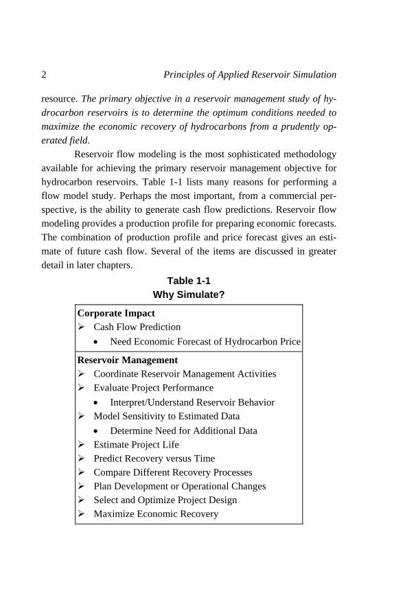
available for achieving the primary reservoir management objective for hydrocarbon reservoirs. Table 1-1 lists many reasons for performing a flow model study. Perhaps the most important, from a commercial per-spective, is the ability to generate cash flow predictions. Reservoir flow modeling provides a production profile for preparing economic forecasts. The combination of production profile and price forecast gives an esti-mate of future cash flow. Several of the items are discussed in greater detail in later chapters.
Table 1-1 Why Simulate?
Corporate Impact Ü Cash Flow Prediction
• Need Economic Forecast of Hydrocarbon Price
Reservoir Management Ü Coordinate Reservoir Management Activities Ü Evaluate Project Performance
• Interpret/Understand Reservoir Behavior Ü Model Sensitivity to Estimated Data
• Determine Need for Additional Data Ü Estimate Project Life Ü Predict Recovery versus Time Ü Compare Different Recovery Processes Ü Plan Development or Operational Changes Ü Select and Optimize Project Design Ü Maximize Economic Recovery

Introduction to Reservoir Management 3
1.1 Consensus Modeling Reservoir flow modeling is the application of a computer simu-lation system to the description of fluid flow in a reservoir [for example, see Peaceman, 1977; Aziz and Settari, 1979; Mattax and Dalton, 1990; Munka and Pápay, 2001; Ertekin, et al., 2001; Carlson, 2003]. The com-puter simulation system is usually just one or more computer programs. To minimize confusion in this text, the computer simulation system is called the reservoir simulator, and the input data set is called the reser-voir flow model. In the modern literature, the term “reservoir model” often refers to the geologic model of a reservoir. The flow simulator has been the point of contact between disci-plines for decades [e.g. see Craig, et al., 1977; and Harris and Hewitt, 1977]. It serves as a filter that selects from among all of the proposed descriptions of the reservoir. The simulator is not influenced by hand-waving arguments or presentation style. It provides an objective ap-praisal of each hypothesis, and constrains the power of personal influence described by Millheim [1997]. As a filter of hypotheses, the reservoir flow modeling team is often the first to know when a proposed hypothesis about the reservoir is inadequate.
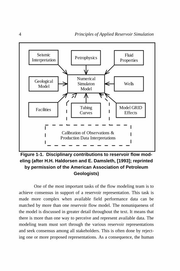
Many different disciplines contribute to the preparation of the input data set of a flow model. The information is integrated during the reservoir flow modeling process, and the concept of the reservoir is quantified in the reservoir simulator. Figure 1-1 illustrates the contribu-tions different disciplines make to reservoir flow modeling. One of the goals of recent technology development is to improve the software used to integrate data from different disciplines and to prepare shared earth models [Cope, 2001; Tearpock and Brenneke, 2001]. Many of the fea-tures of the simulator provided with this text are designed to enhance the integration of data from different disciplines. Fanchi [2002a] presents additional discussion of shared earth models and associated references.
4 Principles of Applied Reservoir Simulation
PetrophysicsSeismic
Interpretation
NumericalSimulaton
Model
GeologicalModel
Facilities
Wells
FluidProperties
TubingCurves
Model GRIDEffects
Calibration of Observations &Production Data Interpretations
Figure 1-1. Disciplinary contributions to reservoir flow mod-eling (after H.H. Haldorsen and E. Damsleth, [1993]; reprinted
by permission of the American Association of Petroleum Geologists)
One of the most important tasks of the flow modeling team is to achieve consensus in support of a reservoir representation. This task is made more complex when available field performance data can be matched by more than one reservoir flow model. The nonuniqueness of the model is discussed in greater detail throughout the text. It means that there is more than one way to perceive and represent available data. The modeling team must sort through the various reservoir representations and seek consensus among all stakeholders. This is often done by reject-ing one or more proposed representations. As a consequence, the human

Introduction to Reservoir Management 5
element is a factor in the process, particularly when the data do not clearly support the selection of a single reservoir representation from a set of competing representations. The dual criteria of reasonableness and Ockham’s Razor [Jefferys and Berger, 1992] are essential to this process, as is an understanding of how individuals can most effectively contribute to the modeling effort.
1.2 Management of Simulation Studies Modern simulation studies of major fields are performed by teams of specialists from different disciplines. The teams of specialists function as project teams in a matrix management organization. Matrix management is synonymous here with Project Management and has two distinct characteristics:
Ü “Cross-functional organization with members from different work areas who take on a project.” [Staff-JPT, 1994]
Ü “One employee is accountable to two or more superiors, which can cause difficulties for managers and employees.” [Staff-JPT, 1994]
According to Maddox [1988], teams and groups differ in the way they behave. Group behavior exhibits the following characteristics:
Ü “Members think they are grouped together for administrative purposes only. Individuals work independently, sometimes at cross purposes.”
Ü “Members tend to focus on themselves because they are not suf-ficiently involved in planning the unit's objectives. They approach their job simply as hired hands.”
By contrast, the characteristics of team behavior are the following: Ü “Members recognize their interdependence and understand both
personal and team goals are best accomplished with mutual sup-

6 Principles of Applied Reservoir Simulation
port. Time is not wasted struggling over territory or seeking per-sonal gain at the expense of others.”
Ü “Members feel a sense of ownership for their jobs and unit be-cause they are committed to goals they helped to establish.”
Haldorsen and Damsleth [1993] have made similar observations: Ü “Members of a team should necessarily understand each other,
respect each other, act as a devil's advocate to each other, and keep each other informed.”
Haldorsen and Damsleth [1993] argue that each team member should focus on innovation and creation of value through the team approach, and on customer orientation that conveys the attitude that “my output is your input.”
Teams need time to develop. Team development proceeds in well known stages [Sears, 1994]:
Ü Introductions: Team members get to know each other. Ü “Storming”: Team members disagree over how to proceed.
• Members can lose sight of goals. Ü “Norming”: Members set standards for team productivity. Ü “Performing”: Team members understand what each member can contribute and how the team works best.
Proper management recognizes these stages and allows time for the team building process to mature.
To alleviate potential problems, the project team should be con-stituted such that each member of the team is assigned a different task,
and all members work toward the same goal. Team members should
have unique roles to avoid redundant functions. If the responsibilities of two or more members of the team overlap considerably, confusion may ensue with regard to areas of responsibility and, by implication, of ac-countability. Each team member must be the key decision maker in a particular discipline, otherwise disputes may not get resolved in the time

Introduction to Reservoir Management 7
available for completing a study. Teams should not be allowed to floun-der in an egalitarian utopia that does not work. McIntosh, et al. [1991] support the notion that each team mem-ber should fulfill a functional role, for example, geoscientist or engineer. A corollary is that team members should be able to understand their roles because the roles have been clearly defined. Wade and Fryer [1997] ob-serve that “getting people to work together as a team rather than a group of individuals can be quite a bit more difficult than it would seem.” They suggest that team members should only include people who spend 100% of their time on areas of responsibility assigned to their team. Bashore [2000] advises that team members should be located close to each other to facilitate communication and cooperation, but cautioned that multidis-ciplinary teams may become microcosms of functionally oriented organizations and never achieve true integration. Effective teams may strive for consensus, but the pressure of meeting deadlines will require one team member to serve as team leader. Deadlines cannot be met if a team cannot agree, and there are many areas where decisions may have to be made without consensus. For this rea-son, teams should have a team leader with significant technical skills and broad experience. Shaw and Morris [2005] add that team leaders should have full management support. This can take the form of technical and monetary authority over the project. If team leaders are perceived as be-ing without authority, they will be unable to fulfill their function. On the other hand, team leaders must avoid exercising authoritarian control or they will weaken the team and wind up with a group. Proper management can improve the likelihood that a team will function as it should. A sense of ownership or “buy-in” can be fostered if team members participate in planning and decision making. Team mem-ber views should influence the work scope and schedule of activity. Many problems can be avoided if realistic expectations are built into pro-ject schedules at the beginning, and then adhered to throughout the

8 Principles of Applied Reservoir Simulation
project. Expanding work scope without altering resource allocation or deadlines can be demoralizing and undermine the team concept. Finally, an important caution should be borne in mind when per-forming studies using teams: “Fewer ideas are generated by groups than by individuals working alone – a conclusion supported by empirical evi-dence from psychology [Norton, 1994].” In describing changes in the work flow of exploration and development studies, Tobias [1998, pg. 38] observes that “asset teams have their drawbacks. The enhanced team-work achieved through a team approach often comes at the expense of individual creativity, as group dynamics can and often does inhibit indi-vidual initiative [Kanter, 1988].” Tobias recommends that organizations allow “the coexistence of both asset teams and individual work environ-ments.” His solution is a work flow that allows the “simultaneous coexistence of decoupled individual efforts and recoupled asset team coordination.”
1.3 “Hands-On” Simulation
The best way to learn how to apply reservoir flow simulators is to get some “hands-on” experience with a real reservoir flow simulator. Consequently, a reservoir flow simulator called IFLO is provided with this text. Many of the terms used in this section to describe IFLO are dis-cussed in more detail in subsequent chapters.
The integrated flow model IFLO is a pseudomiscible, multicom-ponent, multidimensional fluid flow simulator [Fanchi, 2000]. IFLO is called an integrated flow model because it integrates a petrophysical model into a traditional flow simulator. This integration makes it possi-ble to integrate data from such disciplines as geology, geophysics, petrophysics and petroleum engineering in a single software package.
IFLO can be used to model isothermal, Darcy flow in up to three dimensions. It assumes that reservoir fluids can be described by up to

Introduction to Reservoir Management 9
three fluid phases (oil, gas, and water) with physical properties that de-pend on pressure and, to an extent, composition. Natural gas and injected solvent are allowed to dissolve in both the oil and water phases. IFLO includes a petrophysical algorithm that allows the calculation of reser-voir geophysical attributes that make it possible to track changes in seismic variables as a function of time, and to perform geomechanical calculations. A coal gas desorption option is available for modeling coalbed methane production.
IFLO is a modified and significantly expanded version of MAS-TER, a black oil simulator with multicomponent, pseudomiscible options for modeling carbon dioxide or nitrogen flooding [Ammer, et al., 1991]. MASTER is an improved version of BOAST, a reservoir flow simulator that was published by the U.S. Department of Energy in 1982 [Fanchi, et al., 1982]. IFLO includes several enhancements to MASTER, including algorithms from BOAST, its successor BOAST II [Fanchi, et al., 1987], and several new features that are unique to IFLO.
A variety of useful geoscience, geomechanical, and reservoir en-gineering features are available in IFLO. Well modeling features include the representation of horizontal or deviated wells, a well productivity index calculation option, and a stress-dependent permeability model for improving the calculation of well and reservoir flow performance. Petro-physical features include improvements for modeling heterogeneous reservoir characteristics and a petrophysical model for calculating geo-physical and geomechanical properties. The calculation of reservoir geophysical information can be used to model seismic data, including time-lapse seismic surveys. A coal gas production model is also avail-able.
More technical information about the features in IFLO is pro-vided throughout the text. Many of the exercises in the text will help you learn how to use the IFLO options. The exercises guide you through the application of IFLO to a wide range of important reservoir engineering problems.

10 Principles of Applied Reservoir Simulation
1.4 Outline of the Text The remainder of the text is organized as follows. Part I presents a primer on reservoir engineering. The primer is designed to provide background concepts and terminology in the reservoir engineering as-pects of fluid flow in porous media. If you are already familiar with multiphase fluid flow concepts, you should review the exercises in Part I to learn more about IFLO features.
Material in Part II explains the concepts and terminology of res-ervoir flow simulation. Several exercises in Parts I and II use different sections of the user’s manual presented in Part III. A typical exercise asks you to find and change data records in a specified example data file. These records of data must be modified based on an understanding of the reservoir problem and a familiarity with the accompanying computer program IFLO. If you work all the exercises, you will be familiar with the user’s manual and IFLO by the time you have finished. Much of the experience gained by running IFLO is applicable to other flow simula-tors.
Exercises
Exercise 1.1 What is the primary objective of reservoir management? Exercise 1.2 A three-dimensional, three-phase reservoir simulator (IFLO) is included with this book. Prepare a folder on your hard drive for running IFLO using the following procedure.
Copy all IFLO files to a folder on your hard drive before running the simulator. A good name for the folder is “path\IFLO”. Path signifies the drive and directory path to the new folder. Copy all files for this book to the new directory. Some of the files may be labeled “Read Only” when you copy the files to your hard drive. To remove this restriction,

Introduction to Reservoir Management 11
select the file(s) and change the properties of the file(s) by removing the check symbol adjacent to the “Read Only” attribute.
What is the size of the executable file IFLO.EXE in megabytes (MB)?
Exercise 1.3 Several example data files are provided with IFLO. Copy all files to the \IFLO folder on your hard drive using the procedure in Exercise 1.2. Make a list of the data files (files with the extension “dat”). Unless stated otherwise, all exercises assume IFLO and its data files reside in the \IFLO directory. Exercise 1.4 The program IFLO runs the file called “itemp.dat”. To run a new data file, such as newdata.dat, copy newdata.dat to itemp.dat. In this exercise, copy rim_2d.dat to itemp.dat and run IFLO by double clicking on the IFLO.EXE file on your hard drive. Select option “Y” to write the run output to files. When the program ends, it will print “STOP.” Close the IFLO window. You do not need to save changes. Open run output file itemp.rof and find the line reading “MAX # OF AUTHORIZED GRID BLOCKS.” How many gridblocks are you au-thorized to use with the simulator provided with this book? Exercise 1.5 The program 3DVIEW may be used to view the reser-voir structure associated win IFLO data files. 3DVIEW is a visualization program that reads IFLO output files with the extension “arr”. To view a reservoir structure, proceed as follows:
Use your file manager to open your folder containing the IFLO files. Unless stated otherwise, all mouse clicks use the left mouse button. a. Start 3DVIEW (Double click on the application entitled
3DVIEW.EXE) b. Click on the button “File”.

12 Principles of Applied Reservoir Simulation
c. Click on “Open Array File”. d. Click on “ITEMP.ARR” in the file list. e. Click on “OK”.
At this point you should see a structure in the middle of the screen. The structure is an anticlinal reservoir with a gas cap and oil rim. To view different perspectives of the structure, hold the left mouse button down and move the mouse. With practice, you can learn to control the orientation of the structure on the screen.
The gridblock display may be smoothed by clicking on the “Project” button and selecting “Smooth Model Display”. The at-tribute shown on the screen is pressure “P”. To view other attributes, click on the “Model” button, set the cursor on “Select Active Attribute” and then click on oil saturation “SO”. The oil rim should be visible on the screen.
To exit 3DVIEW, click on the “File” button and then click “Exit”.

13
Chapter 2
Basic Reservoir Analysis The tasks associated with basic reservoir analyses provide in-formation that is needed to prepare input data for a simulation study. These tasks include volumetric analysis, material balance analysis, and decline curve analysis. In addition to providing estimates of fluids in place and forecasts of fieldwide production, they also provide an initial concept of the reservoir which can be used to design a model study. Each of these tasks is outlined below.
2.1 Volumetrics Fluid volumes in a reservoir are values that can be obtained from a variety of sources, and therefore serve as a quality control point at the interface between disciplines. Volumetric analysis is used to determine volume from static information [see, for example, Tearpock, et al. 2002; Dake, 2001; Towler, 2002; Walsh and Lake, 2003; Craft, et al., 1991; Mian, 1992]. Static information is information that is relatively constant with respect to time, such as reservoir volume and original saturation and pressure distributions. By contrast, dynamic information such as pressure changes and fluid production is information that changes with respect to time. Material balance and reservoir flow modeling techniques use dy-namic data to obtain original fluid volumes. An accurate characterization of the reservoir should yield consistent estimates of fluid volumes that
14 Principles of Applied Reservoir Simulation
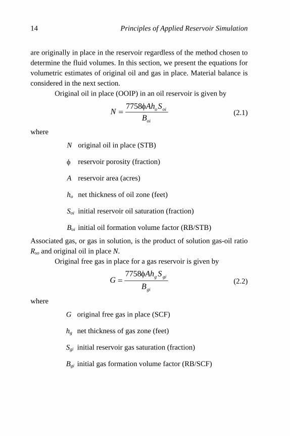
are originally in place in the reservoir regardless of the method chosen to determine the fluid volumes. In this section, we present the equations for volumetric estimates of original oil and gas in place. Material balance is considered in the next section. Original oil in place (OOIP) in an oil reservoir is given by
oi
oio
B
SAhN
φ=
7758 (2.1)
where
N original oil in place (STB)
φ reservoir porosity (fraction)
A reservoir area (acres)
ho net thickness of oil zone (feet)
Soi initial reservoir oil saturation (fraction)
Boi initial oil formation volume factor (RB/STB)
Associated gas, or gas in solution, is the product of solution gas-oil ratio Rso and original oil in place N. Original free gas in place for a gas reservoir is given by
gi
gig
B
SAhG
φ=
7758 (2.2)
where
G original free gas in place (SCF)
hg net thickness of gas zone (feet)
Sgi initial reservoir gas saturation (fraction)
Bgi initial gas formation volume factor (RB/SCF)
Basic Reservoir Analysis 15
Equation (2.2) is often expressed in terms of initial water saturation Swi
by writing wigi SS −=1 . Initial water saturation is usually determined
by well log or core analysis.
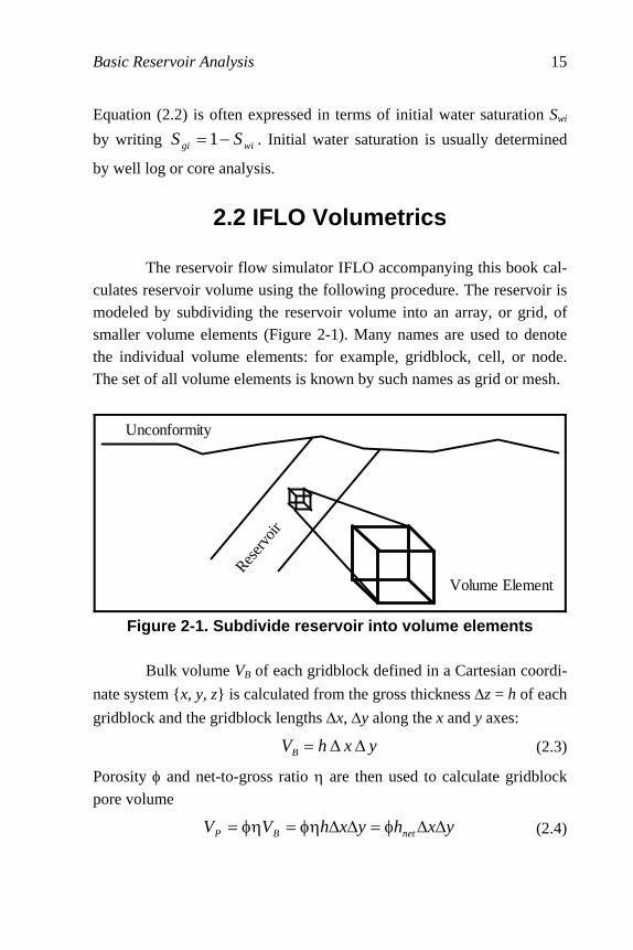
2.2 IFLO Volumetrics The reservoir flow simulator IFLO accompanying this book cal-culates reservoir volume using the following procedure. The reservoir is modeled by subdividing the reservoir volume into an array, or grid, of smaller volume elements (Figure 2-1). Many names are used to denote the individual volume elements: for example, gridblock, cell, or node. The set of all volume elements is known by such names as grid or mesh.
Unconformity
Volume Element
Reser
voir
Figure 2-1. Subdivide reservoir into volume elements
Bulk volume VB of each gridblock defined in a Cartesian coordi-
nate system {x, y, z} is calculated from the gross thickness ∆z = h of each
gridblock and the gridblock lengths ∆x, ∆y along the x and y axes:
yxhVB ∆∆= (2.3)
Porosity φ and net-to-gross ratio η are then used to calculate gridblock
pore volume
yxhyxhVV netBP ∆∆φ=∆∆φη=φη= (2.4)
16 Principles of Applied Reservoir Simulation
where net thickness is defined by hnet = ηh. The volume of phase l in
the gridblock at reservoir conditions is the product of the gridblock pore volume and phase saturation, thus
yxhSVSV netP ∆∆φ== lll (2.5)
where lS is the saturation of phase l . Total model volumes are calcu-
lated by summing over all gridblocks. A comparison of reservoir simulator calculated volumetrics with volumetrics from another source, such as a material balance study or a computer mapping package, provides a means of validating volumetric estimates using independent sources.
2.3 Material Balance The law of conservation of mass is the basis of material balance calculations. Material balance is an accounting of material entering or leaving a system. The calculation treats the reservoir as a large tank of material and uses quantities that can be measured to determine the amount of a material that cannot be directly measured. Measurable quan-tities include cumulative fluid production volumes for oil, water, and gas phases; accurate reservoir pressures; and fluid property data from sam-ples of produced fluids. Material balance calculations may be used for several purposes. They provide an independent method of estimating the volume of oil, water and gas in a reservoir for comparison with volumetric estimates. The magnitude of various factors in the material balance equation indi-cates the relative contribution of different drive mechanisms at work in the reservoir. Material balance can be used to predict future reservoir performance and aid in estimating cumulative recovery efficiency. More discussion of these topics can be found in references such as Dake [2001], Craft, et al. [1991], Ahmed [2000], Towler [2002], and Pletcher [2002].
Basic Reservoir Analysis 17
The form of the material balance equation depends on whether the reservoir is predominately an oil reservoir or a gas reservoir. Each of these cases is considered separately.
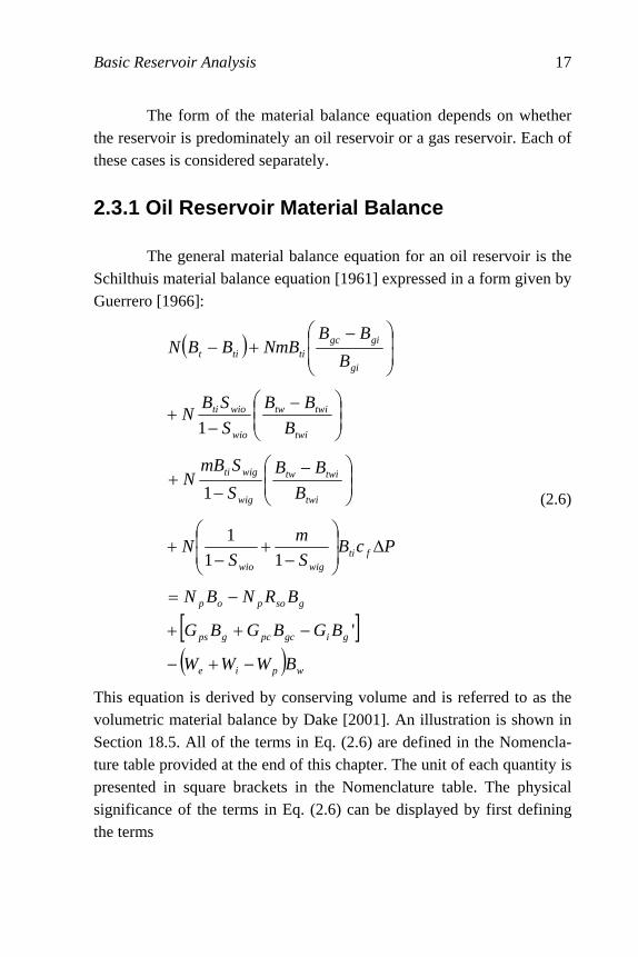
2.3.1 Oil Reservoir Material Balance The general material balance equation for an oil reservoir is the Schilthuis material balance equation [1961] expressed in a form given by Guerrero [1966]:
( )
[ ]( ) wpie
gigcpcgps
gsopop
ftiwigwio
twi
twitw
wig
wigti
twi
twitw
wio
wioti
gi
gigctitit
BWWW
BGBGBG
BRNBN
PcBS
m
SN
B
BB
S
SmBN
B
BB
S
SBN
B
BBNmBBBN
−+−
−++
−=
∆⎟⎟⎠
⎞⎜⎜⎝
⎛
−+
−+
⎟⎟⎠
⎞⎜⎜⎝
⎛ −−
+
⎟⎟⎠
⎞⎜⎜⎝
⎛ −−
+
⎟⎟⎠
⎞⎜⎜⎝
⎛ −+−
'
11
1
1
1
(2.6)
This equation is derived by conserving volume and is referred to as the volumetric material balance by Dake [2001]. An illustration is shown in Section 18.5. All of the terms in Eq. (2.6) are defined in the Nomencla-ture table provided at the end of this chapter. The unit of each quantity is presented in square brackets in the Nomenclature table. The physical significance of the terms in Eq. (2.6) can be displayed by first defining the terms
18 Principles of Applied Reservoir Simulation
PcBS
m
SD
B
BB
S
SmBD
B
BB
S
SBD
B
BBmBD
BBD
ftiwigwio
r
twi
twitw
wig
wigtigw
twi
twitw
wio
wiotiw
gi
gigctigo
tito
∆⎟⎟
⎠
⎞
⎜⎜
⎝
⎛
−+
−=
⎟⎟⎠
⎞⎜⎜⎝
⎛ −−
=
⎟⎟⎠
⎞⎜⎜⎝
⎛ −−
=
⎟⎟
⎠
⎞
⎜⎜
⎝
⎛ −=
−=
11
1
,1
,1
,
,
(2.7)
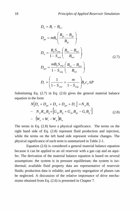
Substituting Eq. (2.7) in Eq. (2.6) gives the general material balance equation in the form
[ ][ ]
( ) wpie
gigcpcgpsgsop
oprgwwgoo
BWWW
BGBGBGBRN
BNDDDDDN
−+−
−++−
=++++
' (2.8)
The terms in Eq. (2.8) have a physical significance. The terms on the right hand side of Eq. (2.8) represent fluid production and injection, while the terms on the left hand side represent volume changes. The physical significance of each term is summarized in Table 2-1. Equation (2.6) is considered a general material balance equation because it can be applied to an oil reservoir with a gas cap and an aqui-fer. The derivation of the material balance equation is based on several assumptions: the system is in pressure equilibrium; the system is iso-thermal; available fluid property data are representative of reservoir fluids; production data is reliable; and gravity segregation of phases can be neglected. A discussion of the relative importance of drive mecha-nisms obtained from Eq. (2.6) is presented in Chapter 7.

Basic Reservoir Analysis 19
Table 2-1 Physical Significance of Material Balance Terms
Term Physical Significance
NDo Change in volume of initial oil and associated gas
NDgo Change in volume of free gas
N(Dw + Dgw) Change in volume of initial connate water
NDr Change in formation pore volume
NpBo Cumulative oil production
NpRsoBg Cumulative gas produced in solution with oil
GpsBg Cumulative solution gas produced as evolved gas
GpcBgc Cumulative gas cap gas production
GiBg′ Cumulative gas injection
WeBw Cumulative water influx
WiBw Cumulative water injection
WpBw Cumulative water production
2.3.2 Gas Reservoir Material Balance The general material balance equation for a gas reservoir can be derived from Eq. (2.6) by first recognizing that the relationship
tigi NmBGB = (2.9)
defines original gas in place G. Substituting Eq. (2.9) into Eq. (2.6) gives the general material balance equation

20 Principles of Applied Reservoir Simulation
( )
[ ]( ) wpiegsop
gigcpcgpsop
fwig
gi
wio
ti
twi
twitw
wig
wiggi
twi
twitw
wio
wioti
gi
gigcgitit
BWWWBRN
'BGBGBGBN
PcS
GB
S
NB
B
BB
S
SBG
B
BB
S
SBN
B
BBGBBBN
−+−−
−++=
∆⎟⎟
⎠
⎞
⎜⎜
⎝
⎛
−+
−+
⎟⎟⎠
⎞⎜⎜⎝
⎛ −−
+
⎟⎟⎠
⎞⎜⎜⎝
⎛ −−
+
⎟⎟
⎠
⎞
⎜⎜
⎝
⎛ −+−
11
1
1
(2.10)
Equation (2.10) is further simplified by recognizing that the material bal-ance for a gas reservoir does not include oil in place so that N = 0 and Np = 0. The resulting material balance equation is
[ ]
( ) wpie
gigcpcf
wig
gi
twi
twitw
wig
wiggi
gi
gigcgi
BWWW
BGBGPcS
GB
B
BB
S
SBG
B
BBGB
−+−
−=∆⎟⎟⎠
⎞⎜⎜⎝
⎛
−+
⎟⎟⎠
⎞⎜⎜⎝
⎛ −−
+⎟⎟⎠
⎞⎜⎜⎝
⎛ −
'1
1
(2.11)
Water compressibility and formation compressibility are relatively small compared to gas compressibility. Consequently, Eq. (2.11) is often writ-ten in the simplified form
[ ]
( ) wpie
gigcpc
gi
gigcgi
BWWW
BGBGB
BBGB
−+−
−=⎟⎟⎠
⎞⎜⎜⎝
⎛ −'
(2.12)
Basic Reservoir Analysis 21
2.4 Decline Curve Analysis Arps [1945] studied the relationship between flow rate and time for producing wells. Assuming constant flowing pressure, he found the relationship:
1+−= naqdt
dq (2.13)
where a and n are empirically determined constants. The empirical con-stant n ranges from 0 to 1. Solutions to Eq. (2.13) show the expected decline in flow rate as the production time increases. Fitting an equation of the form of Eq. (2.13) to flow rate data is referred to as decline curve analysis. Three decline curves have been identified based on the value of n. The exponential decline curve corresponds to n = 0. It has the solution
ati eqq −= (2.14)
where qi is initial rate and a is a factor that is determined by fitting Eq. (2.14) to well or field data. The hyperbolic decline curve corresponds to a value of n in the range 0 < n < 1. The rate solution has the form
ni
n qnatq −− += (2.15)
where qi is initial rate and a is a factor that is determined by fitting Eq. (2.15) to well or field data. The harmonic decline curve corresponds to n = 1. The rate solu-tion is equivalent to Eq. (2.15) with n = 1, thus
11 −− += iqnatq (2.16)
where qi is initial rate and a is a factor that is determined by fitting Eq. (2.16) to well or field data. Decline curves are fit to actual data by plotting the logarithm of observed rates versus time t. The semilog plot yields the following equa-tion for exponential decline:

22 Principles of Applied Reservoir Simulation
atqq i −= lnln (2.17)
Equation (2.17) has the form y = mx + b for a straight line with slope m and intercept b. In the case of exponential decline, time t corresponds to
the independent variable x, qln corresponds to the dependent variable y,
iqln is the intercept b, and –a is the slope m of the straight line. Cumu-
lative production for decline curve analysis is the integral of the rate from the initial rate qi at time t = 0 to the rate q at time t. For example, the cumulative production for the exponential decline case is
a
qqdtqN i
t
p
−== ∫
0
(2.18)
The decline factor a is for the exponential decline case and is found by rearranging Eq. (2.17), thus
iq
q
ta ln
1−= (2.19)
2.5 IFLO Application: Depletion of a Gas Reservoir
The material balance equation for a depletion drive gas reservoir
can be derived from Eq. (2.12). The equation is
( ) ( )[ ]
( )iti
pc ZP
GZPZPG
×−= (2.20)
where G is original free gas in place, Gpc is cumulative free gas pro-duced, P is reservoir pressure and Z is the real gas compressibility factor. Subscript t indicates that the ratio P/Z should be calculated at the time t that corresponds to Gpc and subscript i indicates that the ratio P/Z should be calculated at the initial time. The units of Gpc and G must agree for the equation to be consistent. Equation (2.20) can be used to validate the gas reservoir model-ing features of a reservoir flow simulator such as IFLO if the flow
Basic Reservoir Analysis 23
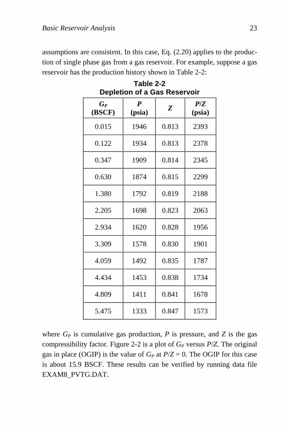
assumptions are consistent. In this case, Eq. (2.20) applies to the produc-tion of single phase gas from a gas reservoir. For example, suppose a gas reservoir has the production history shown in Table 2-2:
Table 2-2 Depletion of a Gas Reservoir
GP (BSCF)
P (psia)
Z P/Z (psia)
0.015 1946 0.813 2393
0.122 1934 0.813 2378
0.347 1909 0.814 2345
0.630 1874 0.815 2299
1.380 1792 0.819 2188
2.205 1698 0.823 2063
2.934 1620 0.828 1956
3.309 1578 0.830 1901
4.059 1492 0.835 1787
4.434 1453 0.838 1734
4.809 1411 0.841 1678
5.475 1333 0.847 1573
where GP is cumulative gas production, P is pressure, and Z is the gas compressibility factor. Figure 2-2 is a plot of GP versus P/Z. The original gas in place (OGIP) is the value of GP at P/Z = 0. The OGIP for this case is about 15.9 BSCF. These results can be verified by running data file EXAM8_PVTG.DAT.

24 Principles of Applied Reservoir Simulation
Figure 2-2. P/Z Plot for Depletion of a Gas Reservoir
Exercises Exercise 2.1 Data file EXAM1.DAT is a material balance model of an undersaturated oil reservoir undergoing pressure depletion. Copy file EXAM1.DAT to file ITEMP.DAT and run IFLO. What are the volumes of initial fluids in place in the model? Hint: Open the run output file ITEMP.ROF to find initial fluids in place. Exercise 2.2 Derive the material balance equation for a system with no gas cap beginning with Eqs. (2.6) and (2.7). Exercise 2.3 Derive Eq. (2.18) for the exponential decline case by using Eq. (2.14) as the integrand and performing the integration. Exercise 2.4A A formation consists of 20 feet of impermeable shale and 80 feet of permeable sandstone. What is the gross thickness of the forma-tion? Exercise 2.4B What is the net-to-gross ratio of the formation?
0
500
1000
1500
2000
2500
3000
0 2 4 6 8 10 12 14 16 18
Gp (BSCF)P/Z (psia)

Basic Reservoir Analysis 25
Exercise 2.5A Show that q q eiat= − is a solution of the decline curve
equation dq dt aqn= − +1 for the exponential decline case.
Exercise 2.5B Plot oil flow rate as a function of time for a well that pro-duces 10,000 barrels per day with a decline factor a = 0.06 per year. Time should be expressed in years, and should range from 0 to 50 years. Exercise 2.5C When does the flow rate drop below 1000 barrels per day?
Exercise 2.6A Show that q at qi− −= +1 1 is a solution of
dq
dtaq= − 2
where a qi, are constants?
Exercise 2.6B What is the value of q at t = 0?
Exercise 2.7 A barrier island is a large sand body. Consider a barrier island that averages 3 miles wide, 10 miles long, and is 30 feet thick. The porosity of the sand averages almost 25%. What is the pore volume of the barrier island? Express your answer in barrels and cubic meters. Exercise 2.8 Use Eq. (2.12) to derive Eq. (2.20). Exercise 2.9A The results shown in Table 2-2 were obtained from data file EXAM8_PVTG.DAT. Verify that the OGIP for the model is about 15.9 BSCF by running EXAM8_PVTG.DAT and finding the OGIP in WTEMP.ROF. How much oil and water were originally in place? Exercise 2.9B Assume that the reservoir with the production history given in Table 2-2 is abandoned at pressure Pa = 1657 psia with Za = 0.826. Estimate cumulative gas production at abandonment from a graph of P/Z versus Gp (Figure 2-2).

26 Principles of Applied Reservoir Simulation
Exercise 2.9C Run EXAM8_PVTG.DAT and determine the cumulative gas production at a pressure of 1657 psia from the timestep summary file ITEMP.TSS. How does this result compare to the value of cumulative gas production found in Part B?
Nomenclature for Equation (2.6)
Bg Bgc Bg' Bo Bt Btw cf G Gi Gpc Gps m N Np Rso Rsi Rsw Rswi Sg So Sw Swi Swig Swio We Wi Wp ∆P Pi P
gas formation volume factor (FVF) (RB/SCF) gas cap FVF (RB/SCF) injected gas FVF (RB/SCF) oil FVF (RB/STB) Bo + (Rsi - Rso)Bg = composite oil FVF (RB/STB) Bw + (Rswi - Rsw)Bg = composite water FVF (RB/STB) formation (rock) compressibility (1/psia) initial gas in place (SCF) cumulative gas injected (SCF) cumulative gas cap gas produced (SCF) cumulative solution gas produced as evolved gas (SCF) ratio of gas reservoir volume to oil reservoir volume initial oil in place (STB) cumulative oil produced (STB) solution gas-oil ratio (SCF/STB) initial solution gas-oil ratio (SCF/STB) solution gas-water ratio (SCF/STB) initial solution gas-water ratio (SCF/STB) gas saturation (fraction) oil saturation (fraction) water saturation (fraction) initial water saturation (fraction) initial water saturation in gas cap (fraction) initial water saturation in oil zone (fraction) cumulative water influx (STB) cumulative water injected (STB) cumulative water produced (STB) Pi - P = reservoir pressure change (psia) initial reservoir pressure (psia) reservoir pressure corresponding to cumulative fluid times (psia)
27
Chapter 3
Multiphase Flow Concepts Several basic concepts are needed to understand multiphase flow. They include interfacial tension, wettability, and contact angle. These concepts lead naturally to a discussion of capillary pressure, mo-bility, and fractional flow.
3.1 Basic Concepts The concepts of interfacial tension, wettability, and contact angle describe the behavior of two or more phases in relation to one another. They are defined here and then applied in later sections.
3.1.1 Interfacial Tension On all interfaces between solids and fluids, and between immis-cible fluids, there is a surface free energy resulting from electrical forces. These forces cause the surface of a liquid to occupy the smallest possible area and act like a membrane. Interfacial tension (IFT) refers to the ten-sion between liquids at a liquid-liquid interface. Surface tension refers to the tension between fluids at a gas-liquid interface. Interfacial tension is energy per unit of surface area, or force per unit length. The units of IFT are typically expressed in milli-Newtons per meter or the equivalent dynes per centimeter. The value of IFT depends
28 Principles of Applied Reservoir Simulation
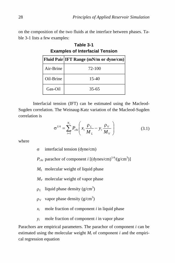
on the composition of the two fluids at the interface between phases. Ta-ble 3-1 lists a few examples:
Table 3-1 Examples of Interfacial Tension
Fluid Pair IFT Range (mN/m or dyne/cm)
Air-Brine 72-100
Oil-Brine 15-40
Gas-Oil 35-65
Interfacial tension (IFT) can be estimated using the Macleod-Sugden correlation. The Weinaug-Katz variation of the Macleod-Sugden correlation is
⎟⎟⎠
⎞⎜⎜⎝
⎛ ρ−
ρ=σ ∑
= V
Vi
L
Li
N
iich M
yM
xPc
1
41 (3.1)
where
σ interfacial tension (dyne/cm)
Pchi parachor of component i [(dynes/cm)1/4/(g/cm3)]
ML molecular weight of liquid phase
MV molecular weight of vapor phase
ρL liquid phase density (g/cm3)
ρV vapor phase density (g/cm3)
xi mole fraction of component i in liquid phase
yi mole fraction of component i in vapor phase
Parachors are empirical parameters. The parachor of component i can be estimated using the molecular weight Mi of component i and the empiri-cal regression equation
Multiphase Flow Concepts 29
iich MP 92.20.10 += (3.2)
This procedure works reasonably well for molecular weights ranging from 100 to 500. A more accurate procedure for a wider range of mo-lecular weights is given by Fanchi [1990].
3.1.2 Wettability
Wettability is the ability of a fluid phase to wet a solid surface preferentially in the presence of a second immiscible phase. The wetting, or wettability, condition in a rock/fluid system depends on IFT. Chang-ing the type of rock or fluid can change IFT and, hence, the wettability of the system. Adding a chemical such as surfactant, polymer, corrosion inhibitor, or scale inhibitor can alter wettability.
3.1.3 Contact Angle Wettability is measured by contact angle. Contact angle is al-ways measured through the denser phase and is related to interfacial energies by
θσ=σ−σ cosowwsos (3.3)
where
σos interfacial energy between oil and solid (dyne/cm)
σws interfacial energy between water and solid (dyne/cm)
σow interfacial energy, or IFT, between oil and water (dyne/cm)
θ contact angle at oil-water-solid interface measured throughthe water phase (degrees)
Table 3-2 presents examples of contact angle for different wetting condi-tions.

30 Principles of Applied Reservoir Simulation
Table 3-2 Examples of Contact Angle
Wetting Condition Contact Angle
(Degrees)
Strongly water-wet 0-30
Moderately water-wet 30-75
Neutrally wet 75-105
Moderately oil-wet 105-150
Strongly oil-wet 150-180
Wettability is usually measured in the laboratory. Several factors
can affect laboratory measurements of wettability. Wettability can be changed by contact of the core during coring with drilling fluids or fluids on the rig floor, and by contact of the core during core handling with oxygen or water from the atmosphere. Laboratory fluids should also be at reservoir conditions to obtain the most reliable measurements of wet-tability. For example, a wettability measurement for an oil-water system should, in principle, use oil with dissolved gas at reservoir temperature and pressure. Based on laboratory tests, most known reservoirs have in-termediate wettability and are preferentially water wet.
3.2 Capillary Pressure
Capillary pressure is the pressure difference across the curved interface formed by two immiscible fluids in a small capil-lary tube. The pressure difference is
wnwc PPP −= (3.4)
where
Multiphase Flow Concepts 31
Pc capillary pressure (psi)
Pnw pressure in nonwetting phase (psi)
Pw pressure in wetting phase (psi)
3.2.1 Capillary Pressure Theory Equilibrium between fluid phases in a capillary tube is sat-isfied by the relationship force up = force down. These forces are expressed in terms of the radius r of the capillary tube, the contact
angle θ, and the interfacial tension σ. The forces are given by
force up = IFT acting around perimeter of capillary tube
= σ cos θ × 2πr
and
force down =density gradient difference × cross-sectionalarea × height h of capillary rise in tube
The density gradient Γ is the weight of the fluid per unit length per unit cross-sectional area. For example, the density gradient of wa-
ter Γw is approximately 0.433 psia/ft at standard conditions. If we assume an air-water system, the force down is
force down =(Γw - Γair)πr 2h
where the cross-sectional area of the capillary tube is πr2. Capil-lary pressure Pc is defined as the force per unit area, thus
Pc = force up / πr 2 = force down / πr 2.
3.2.2 Capillary Pressure and Pore Radius Expressing capillary pressure in terms of force up per unit area gives:

32 Principles of Applied Reservoir Simulation
rr
rPc
θσ=
πθσπ
=cos2cos2
2 (3.5)
where
r pore radius (cm)
σ interfacial (or surface) tension (mN/m or dynes/cm)
θ contact angle (degrees)
Equation (3.5) shows that an increase in pore radius will cause a reduction in capillary pressure while a decrease in IFT will cause a decrease in capillary pressure.
3.2.3 Equivalent Height Expressing Pc in terms of force down leads to the expres-sion
( ) ( )airw
airwc h
r
hrP Γ−Γ=
πΓ−Γπ
=2
2
(3.6)
where h height of capillary rise (ft)
Pc capillary pressure (psia)
Γw water, or wetting phase, density gradient (psia/ft)
Γair air, or nonwetting phase, density gradient (psia/ft)
Solving for h yields the defining relationship between capillary
pressure Pc and equivalent height h, namely
( )airw
cPh
Γ−Γ= (3.7)
The equivalent height is the height above the free fluid level of the wetting phase, where the free fluid level is the elevation of the

Multiphase Flow Concepts 33
wetting phase at 0=cP . For example, Ahmed [2000, pages 206-
208] defines free water level as the elevation where capillary pres-sure equals zero at 100% water saturation and the water-oil contact is the uppermost depth in the reservoir where water saturation is 100%. Figure 3-1 illustrates these definitions.
Oil Zone
TransitionZone
HeightAboveFWL
Water Saturation
Water ZoneWOC
FWL0.0 ft
0.0 Swc 1.0
Figure 3-1. Sketch of an Oil-Water Transition Zone
Note that WOC is water-oil contact, FWL is free water level, and Swc is irreducible or connate water saturation.
Equivalent height is inversely proportional to the difference
in densities between two immiscible phases. The thickness of the transition zone between the wetting phase and the nonwetting phase is the difference in equivalent height between the wetting phase contact (the uppermost depth in the reservoir where wetting phase saturation is 100%) and the height where the wetting phase saturation is irreducible. For example, the thickness of the oil-water transition zone is the difference in equivalent height between the water-oil contact and the height where water saturation equals irreducible water saturation. The relatively large density difference between gas and liquid phases results in a smaller transition zone
34 Principles of Applied Reservoir Simulation
thickness than the relatively small difference between two liquid phase densities.
The preceding definitions of free fluid level and fluid con-tact are based on capillary pressure. It is also possible to define free fluid level and fluid contact using measurements of formation pressure and pressure gradients in different fluid zones. The mod-eling team should know how free fluid levels and fluid contacts are defined to avoid confusion.
3.2.4 Oil-Water Capillary Pressure Oil is the nonwetting phase in a water-wet oil-water reser-voir. Capillary pressure for an oil-water system is
wocow PPP −= (3.8)
where
Po pressure in the oil phase (psia)
Pw pressure in the water phase (psia)
Capillary pressure increases with height above the oil-water con-tact (OWC) as water saturation decreases.
3.2.5 Gas-Oil Capillary Pressure In gas-oil systems, gas usually behaves as the nonwetting phase and oil is the wetting phase. Capillary pressure between oil and gas in such a system is
ogcgo PPP −= (3.9)
where
Pg pressure in the gas phase (psia)
Multiphase Flow Concepts 35
Po pressure in the oil phase (psia)
Capillary pressure increases with height above the gas-oil contact (GOC) as gas saturation decreases.
3.2.6 Capillary Pressure Correction The proper way to include capillary pressure in a flow model study is to correct laboratory measured values to reservoir conditions. This is done by applying the correction:
( ) ( )( )( )
lab
rescorrcorrlabcresc PP
θσ
θσ≡ηη=
cos
cos, (3.10)
where σ is interfacial tension (IFT), and θ is wettability angle [Amyx, et al., 1960]. The subscripts lab and res refer to laboratory conditions and reservoir conditions respectively. If laboratory measurements of IFT are not available, IFT can be estimated from the Macleod-Sugden correlation for pure compounds or the Wein-aug-Katz correlation for mixtures [Fanchi, 1990].
A problem with the capillary correction in Eq. (3.10) is that it requires data that are often poorly known, namely interfacial ten-sion and wettability contact angle at reservoir conditions. Rao and Girard [1997] have described a laboratory technique for measuring wettability using live fluids at reservoir temperature and pressure. Alternative approaches include adjusting capillary pressure curves to be consistent with well log estimates of transition zone thick-ness, or assuming the contact angle factors out.
3.2.7 Leverett’s J-Function Rock samples with different pore-size distribution, perme-ability, and porosity will yield different capillary pressure curves.
36 Principles of Applied Reservoir Simulation
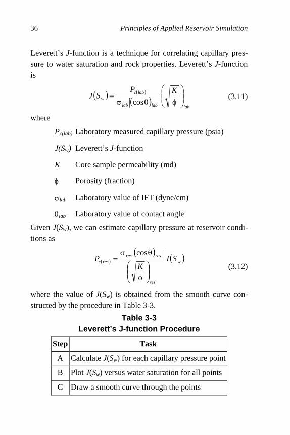
Leverett’s J-function is a technique for correlating capillary pres-sure to water saturation and rock properties. Leverett’s J-function is
( ) ( )
( )lablablab
labcw
KPSJ ⎟⎟
⎠
⎞⎜⎜⎝
⎛
φθσ=
cos (3.11)
where
Pc(lab) Laboratory measured capillary pressure (psia)
J(Sw) Leverett’s J-function
K Core sample permeability (md)
φ Porosity (fraction)
σlab Laboratory value of IFT (dyne/cm)
θlab Laboratory value of contact angle
Given J(Sw), we can estimate capillary pressure at reservoir condi-tions as
( )
( ) ( )w
res
resresresc SJ
KP
⎟⎟⎠
⎞⎜⎜⎝
⎛
φ
θσ=
cos
(3.12)
where the value of J(Sw) is obtained from the smooth curve con-structed by the procedure in Table 3-3.
Table 3-3 Leverett’s J-function Procedure
Step Task
A Calculate J(Sw) for each capillary pressure point
B Plot J(Sw) versus water saturation for all points
C Draw a smooth curve through the points

Multiphase Flow Concepts 37
3.3 Relative Permeability
Relative permeability is used to describe multiphase fluid flow. The general definition of relative permeability is
abs
effr k
kk = (3.13)
where
kr relative permeability between 0 and 1,
keff effective permeability (md)
kabs absolute permeability (md)
Fluid phase relative permeabilities for oil, water and gas phases, respectively, are
kkkkkkkkk grgwrworo === ,, (3.14)
The variable lk is the effective permeability of phase l for sub-
script l denoting oil o , water w , or gas g . The relative
permeability of phase l is lrk , and k is absolute permeability. Fig-
ure 3-2 shows a typical set of relative permeability curves. Changes in the wettability conditions of the core can sig-
nificantly affect relative permeability. Ideally, relative permeability should be measured in the laboratory under the same conditions of wettability that exist in the reservoir. One way to ap-proximate this ideal is to use preserved, native state core samples. In practice, most relative permeability data are obtained using re-stored state cores in the laboratory.
Relative permeability data should be obtained by experi-ments that best model the type of displacement that is thought to dominate reservoir flow performance. For example, water-oil im-bibition curves are representative of waterflooding, while water-oil

38 Principles of Applied Reservoir Simulation
drainage curves describe the movement of oil into a water zone. The dependence of relative permeability on the history of satura-tion changes is called hysteresis. Relative permeability hysteresis effects can be included in some reservoir flow models (for exam-ple, see Killough [1976], Dake [2001], Carlson [2003]).
Relative permeability data are often measured and reported for laboratory analysis of several core samples from one or more wells in a field. The set of relative permeability curves should be sorted by lithology and averaged to determine a representative set of curves for each rock type. Several procedures exist for averag-ing relative permeability data [for example, see Schneider, 1987; Mattax and Dalton, 1990; Blunt, 1999; Fanchi, 2000].
0.0
0.2
0.4
0.6
0.8
1.0
0.0 0.1 0.2 0.3 0.4 0.5 0.6 0.7 0.8 0.9 1.0
Water Saturation (fraction)
Rel
ativ
e P
erm
eab
ility
(fr
actio
n)
krw (imb) kro (drain) kro (imb) Figure 3-2. Typical Water-Oil Relative Permeability Curves
3.4 Mobility and Fractional Flow Mobility is a measure of the ability of a fluid to move through interconnected pore space. Fractional flow is the ratio of the volume of
Multiphase Flow Concepts 39
one phase flowing to the total volume flowing in a multiphase system. These concepts are defined here.
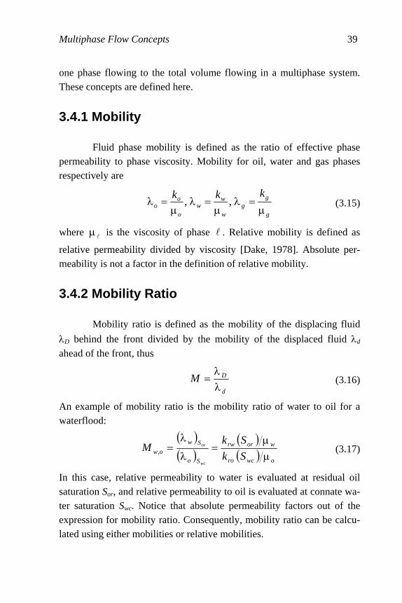
3.4.1 Mobility
Fluid phase mobility is defined as the ratio of effective phase permeability to phase viscosity. Mobility for oil, water and gas phases respectively are
g
gg
w
ww
o
oo
kkk
µ=λ
µ=λ
µ=λ ,, (3.15)
where lµ is the viscosity of phase l . Relative mobility is defined as
relative permeability divided by viscosity [Dake, 1978]. Absolute per-meability is not a factor in the definition of relative mobility.
3.4.2 Mobility Ratio
Mobility ratio is defined as the mobility of the displacing fluid
λD behind the front divided by the mobility of the displaced fluid λd
ahead of the front, thus
d
DMλλ
= (3.16)
An example of mobility ratio is the mobility ratio of water to oil for a waterflood:
( )( )
( )( ) owcro
worrw
So
Sw
ow Sk
SkM
wc
or
µµ
=λ
λ=, (3.17)
In this case, relative permeability to water is evaluated at residual oil saturation Sor, and relative permeability to oil is evaluated at connate wa-ter saturation Swc. Notice that absolute permeability factors out of the expression for mobility ratio. Consequently, mobility ratio can be calcu-lated using either mobilities or relative mobilities.
40 Principles of Applied Reservoir Simulation
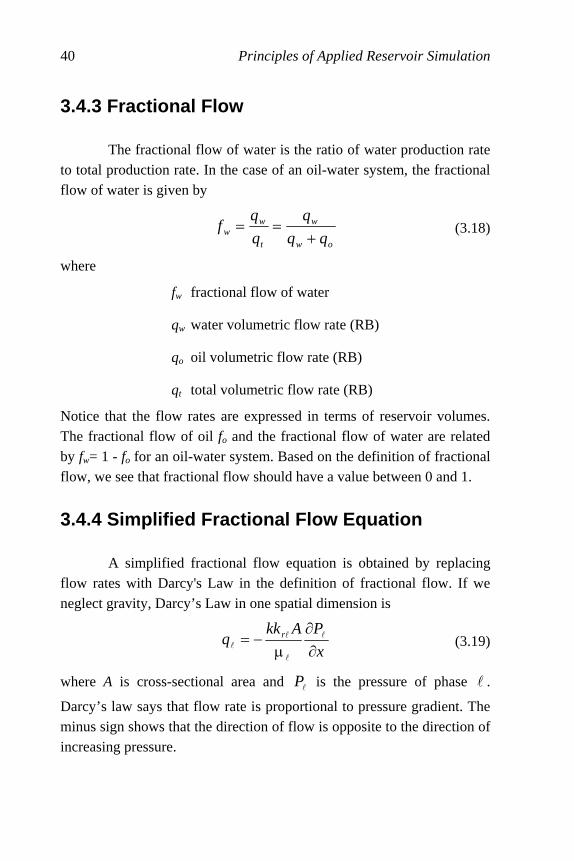
3.4.3 Fractional Flow The fractional flow of water is the ratio of water production rate to total production rate. In the case of an oil-water system, the fractional flow of water is given by
ow
w
t
ww qq
q
q
qf
+== (3.18)
where
fw fractional flow of water
qw water volumetric flow rate (RB)
qo oil volumetric flow rate (RB)
qt total volumetric flow rate (RB)
Notice that the flow rates are expressed in terms of reservoir volumes. The fractional flow of oil fo and the fractional flow of water are related by fw= 1 - fo for an oil-water system. Based on the definition of fractional flow, we see that fractional flow should have a value between 0 and 1.
3.4.4 Simplified Fractional Flow Equation
A simplified fractional flow equation is obtained by replacing flow rates with Darcy's Law in the definition of fractional flow. If we neglect gravity, Darcy’s Law in one spatial dimension is
x
PAkkq r
∂∂
µ−= l
l
ll (3.19)
where A is cross-sectional area and lP is the pressure of phase l .
Darcy’s law says that flow rate is proportional to pressure gradient. The minus sign shows that the direction of flow is opposite to the direction of increasing pressure.
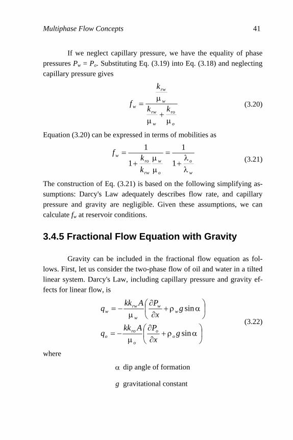
Multiphase Flow Concepts 41
If we neglect capillary pressure, we have the equality of phase pressures Pw = Po. Substituting Eq. (3.19) into Eq. (3.18) and neglecting capillary pressure gives
o
ro
w
rw
w
rw
w kk
k
f
µ+
µ
µ= (3.20)
Equation (3.20) can be expressed in terms of mobilities as
w
o
o
w
rw
row
k
kf
λλ
+=
µµ
+=
1
1
1
1
(3.21)
The construction of Eq. (3.21) is based on the following simplifying as-sumptions: Darcy's Law adequately describes flow rate, and capillary pressure and gravity are negligible. Given these assumptions, we can calculate fw at reservoir conditions.
3.4.5 Fractional Flow Equation with Gravity
Gravity can be included in the fractional flow equation as fol-lows. First, let us consider the two-phase flow of oil and water in a tilted linear system. Darcy's Law, including capillary pressure and gravity ef-fects for linear flow, is
⎟⎠⎞
⎜⎝⎛ αρ+∂∂
µ−=
⎟⎠⎞
⎜⎝⎛ αρ+∂∂
µ−=
sin
sin
gx
PAkkq
gx
PAkkq
oo
o
roo
ww
w
rww
(3.22)
where
α dip angle of formation
g gravitational constant
42 Principles of Applied Reservoir Simulation
If we differentiate capillary pressure for a water-wet system with respect to position x along the dipping bed, we find
x
P
x
P
x
P wocow
∂∂
−∂∂
=∂∂
(3.23)
Combining Eqs. (3.22) and (3.23) gives
( )
αρ+µ
+αρ−µ−
−=∂∂
sinsin gAkk
qg
Akk
x
Pw
w
wwo
ro
owtcow(3.24)
where we have used qt = qo + qw. If we write the density difference as
ow ρ−ρ=ρ∆ (3.25)
collect terms, and simplify we obtain
αρ∆−∂∂
+µ
=⎟⎟⎠
⎞⎜⎜⎝
⎛ µ+
µsing
x
P
Akk
q
kkAk
q cow
ro
ot
rw
w
ro
ow (3.26)
Rearranging and collecting terms gives the fractional flow to water fw in conventional oilfield units:
( )
o
w
rw
ro
owcow
to
ro
t
ww
k
kx
P
q
Akk
q
qf
µµ
+
⎥⎦
⎤⎢⎣
⎡αγ−γ−
∂∂
µ+
=
=
1
sin433.0001127.01 (3.27)
where
A cross-sectional area of flow system (ft2)
k absolute permeability (md)
kro relative permeability to oil
krw relative permeability to water
µo oil viscosity (cp)
µw water viscosity (cp)
Multiphase Flow Concepts 43
Pcow oil-water capillary pressure (psi) = Po - Pw
x direction of linear flow (ft)
α dip angle of formation (degrees)
γo oil specific gravity (pure water = 1)
γw water specific gravity (pure water = 1)
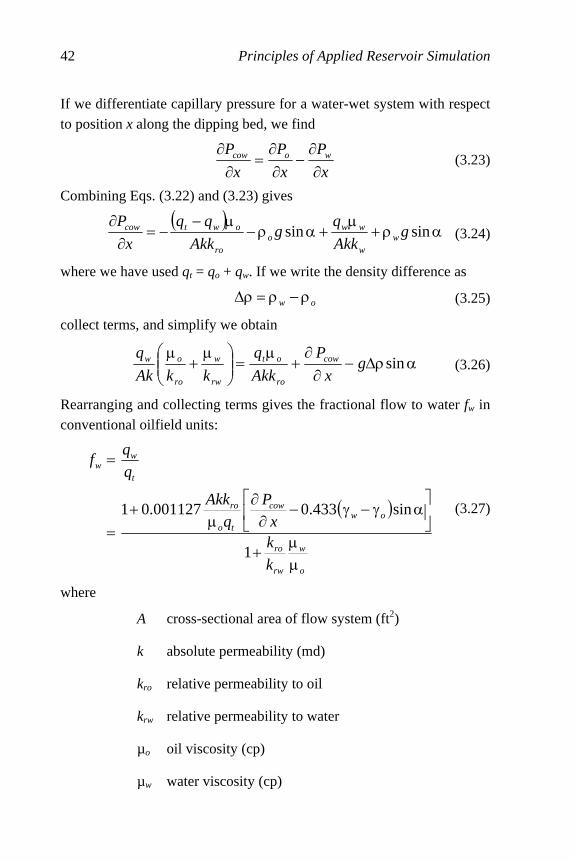
The general expression for fw includes all three terms governing immis-cible displacement, namely the viscous term (kro/krw)(µw/µo), the capillary
pressure term xPcow ∂∂ and the gravity term ( ) αγ−γ sinow .
It is interesting to note that the capillary pressure and gravity terms are multiplied by 1/qt in Eq. (3.27). Most waterfloods have suffi-ciently high flow rates that capillary pressure and gravity effects can be neglected, leaving the simplified expression
o
w
rw
row
k
kf
µµ
+=
1
1
(3.28)
Equation (3.28) is in agreement with Eq. (3.21), as it should be.
3.4.6 Gas Fractional Flow
A similar analysis can be performed to determine the fractional flow of gas fg. The result for a gas-oil system is
( )
o
g
rg
ro
ogcgo
to
ro
g
k
k
x
P
q
Akk
f
µµ
+
⎟⎟⎠
⎞⎜⎜⎝
⎛αγ−γ−
∂∂
′µ+
=1
sin433.0001127.01
(3.29)
where oil phase properties are defined after Eq. (3.27) and the remaining variables are
krg relative permeability to gas
44 Principles of Applied Reservoir Simulation
µg gas viscosity (cp)
Pcgo gas-oil capillary pressure = Pg - Po (psi)
γg gas specific gravity (pure water = 1)
qg gas volumetric flow rate (RB/day)
tq′ total volumetric flow rate = qo + qg (RB/day)
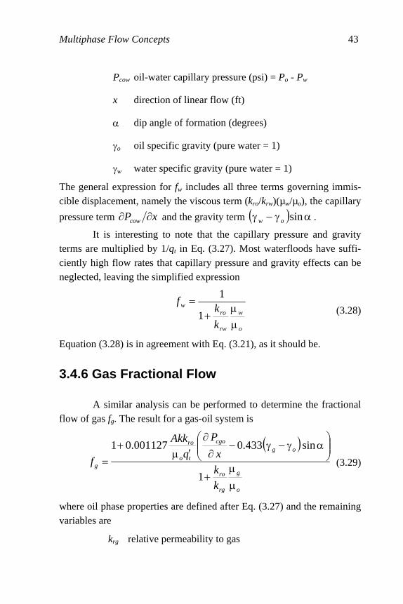
Immiscible displacement of oil by gas is analogous to water displacing oil with the water terms replaced by gas terms. In general, the gravity term in fg should not be neglected unless qt is very high because of the specific gravity difference between gas and oil.
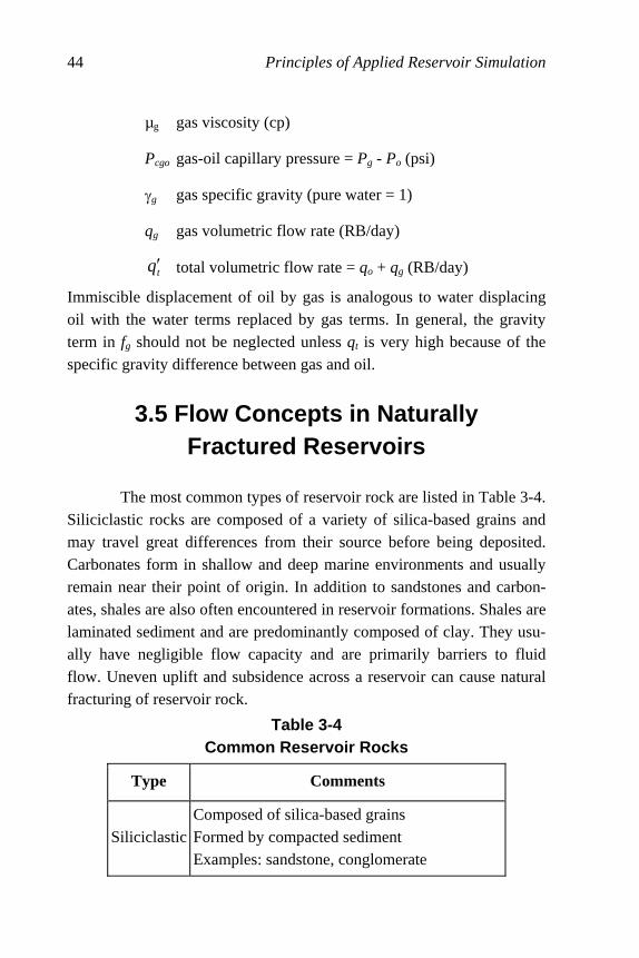
3.5 Flow Concepts in Naturally Fractured Reservoirs
The most common types of reservoir rock are listed in Table 3-4.
Siliciclastic rocks are composed of a variety of silica-based grains and may travel great differences from their source before being deposited. Carbonates form in shallow and deep marine environments and usually remain near their point of origin. In addition to sandstones and carbon-ates, shales are also often encountered in reservoir formations. Shales are laminated sediment and are predominantly composed of clay. They usu-ally have negligible flow capacity and are primarily barriers to fluid flow. Uneven uplift and subsidence across a reservoir can cause natural fracturing of reservoir rock.
Table 3-4 Common Reservoir Rocks
Type Comments
SiliciclasticComposed of silica-based grains Formed by compacted sediment Examples: sandstone, conglomerate

Multiphase Flow Concepts 45
CarbonatesProduced by chemical and biochemical sourcesComposed primarily of calcite and dolomite Examples: limestone, dolostone
Naturally fractured reservoirs are characterized by the juxtaposi-tion of two rock types: reservoir matrix, and fractures. Reservoir matrix rock typically has a larger storage capacity than fractures, but the frac-tures have a larger flow capacity than the reservoir matrix. Bulk volume and porosity are typically larger in matrix rock than in fractures, while fracture permeability is typically much larger than matrix permeability. These characteristics result in two different flow regimes: the matrix flow regime and the fracture flow regime. Table 3-5 presents a classifica-tion of naturally fractured reservoirs based on fluid storage [Aguilera, 1999].
Table 3-5 Naturally Fractured Reservoir Types
Type Storage of Fluid Volume
A In matrix
B In both matrix and fracture
C In fracture
Production from a naturally fractured reservoir depends on both
the matrix flow regime and the fracture flow regime. For example, most of the fluid volume in a Type A naturally fractured reservoir is stored in the matrix, and most of the fluid flow is in the fractures. Figure 3-3 is a sketch of a Type A naturally fractured reservoir with a horizontal frac-ture network. Horizontal fractures can also be created by hydraulic fracturing. The amount of fluid produced depends on how much fluid is in the fracture and the rate at which the fluid can enter the fracture net-work.

46 Principles of Applied Reservoir Simulation
fractures
x
y
z
matrix
Figure 3-3. Sketch of a Naturally Fractured Reservoir with Horizontal Fractures
Production from naturally fractured reservoirs usually occurs
from wells that intersect the network of interconnected fractures. Fluid flow in fractures depends on such factors as aperture size (width or di-ameter of the fracture), fracture orientation, net stress on the fracture, fracture permeability, and recovery mechanisms. Fluid in the matrix is usually recovered by flowing into fractures that are open to flow and in communication with a well. Fracture permeability can be diminished by mineralization. Open fractures have not undergone mineralization. Closed fractures are fractures with no permeability. Many fractures have been subjected to some mineralization and are partially open. Mecha-nisms for recovering fluid from the matrix-fracture system include water drive, capillary imbibition, solution gas drive, gravity drainage, gas cap expansion, and combination drive. Further discussion of recovery mechanisms in naturally fractured reservoirs is provided by Aguilera [1999], Firoozabadi [2000], Allan and Sun [2003], and references therein. These mechanisms depend on fracture capillary pressure and fracture relative permeability.
3.5.1 Fracture Capillary Pressure
Preuss and Tsang [1990] envisioned a fracture as a collection of narrow channels and assumed a log-normal distribution of aperture size.

Multiphase Flow Concepts 47
The most probable aperture size for their log-normal distribution was 0.05 mm. The result of their study was a formula that related capillary pressure and wetting-phase saturation. Their curve for a water-oil system has the form of Leverett’s J-function which is familiar from the study of unfractured porous media.
Firoozabadi and Hauge [1990] used a centrifuge to measure the capillary pressure across the interfaces between stacked matrix blocks. The typical aperture size was about 0.1 mm to 0.2 mm. They obtained a fracture capillary pressure curve for an oil-water system that was ap-proximately represented by Leverett’s J-function in accordance with the work by Preuss and Tsang [1990]. More recent discussions of fracture capillary pressure are presented by Akin [2001], and Deghmoum, et al. [2001].
3.5.2 Fracture Relative Permeability
Fracture apertures can range in size from very small to very large. When fracture apertures are very small, wall roughness and tortu-osity can affect fluid flow. In this case, it is reasonable to assume that two or more flowing phases may interfere with one another as if they were confined to the pore space of an unfractured porous medium. The resulting fracture relative permeability curves will be nonlinear functions of wetting phase saturation [Preuss and Tsang, 1990]. Nonlinear rela-tions between relative permeability and saturation have been observed by several authors, including Persoff, et al. [1991], McDonald, et al. [1991], Akin [2001], and Deghmoum, et al. [2001].
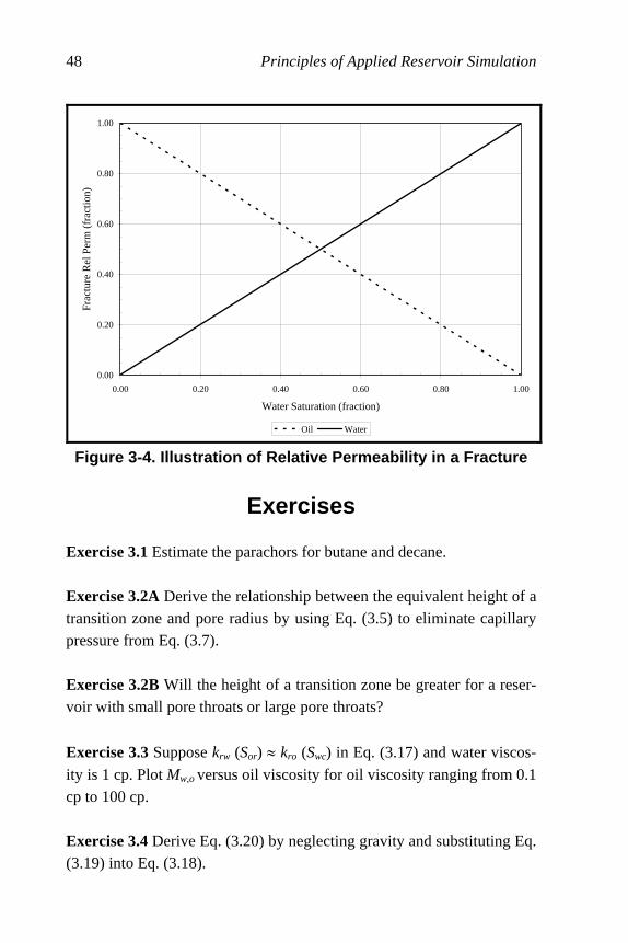
If fracture aperture size is large, two or more fluid phases can flow in the fracture without significantly interfering with each other. The resulting relative permeability curves are approximately straight lines. In the absence of experimental data to the contrary, fracture relative perme-ability and capillary pressure are usually assumed to be linear functions of wetting phase saturation. Fracture relative permeability curves are illustrated in Figure 3-4 for an oil-water system.
48 Principles of Applied Reservoir Simulation
0.00
0.20
0.40
0.60
0.80
1.00
0.00 0.20 0.40 0.60 0.80 1.00
Water Saturation (fraction)
Fra
ctu
re R
el P
erm
(fr
actio
n)
Oil Water
Figure 3-4. Illustration of Relative Permeability in a Fracture
Exercises Exercise 3.1 Estimate the parachors for butane and decane. Exercise 3.2A Derive the relationship between the equivalent height of a transition zone and pore radius by using Eq. (3.5) to eliminate capillary pressure from Eq. (3.7). Exercise 3.2B Will the height of a transition zone be greater for a reser-voir with small pore throats or large pore throats?
Exercise 3.3 Suppose krw (Sor) ≈ kro (Swc) in Eq. (3.17) and water viscos-
ity is 1 cp. Plot Mw,o versus oil viscosity for oil viscosity ranging from 0.1 cp to 100 cp. Exercise 3.4 Derive Eq. (3.20) by neglecting gravity and substituting Eq. (3.19) into Eq. (3.18).

Multiphase Flow Concepts 49
Exercise 3.5 Derive Eq. (3.24) from Eqs. (3.22) and (3.23). Exercise 3.6 Suppose the density gradient for water is 0.43 psia/ft and the density gradient for oil is 0.35 psia/ft. What is the equivalent height of a water-oil transition zone if capillary pressure is 16 psia? Exercise 3.7A Oil recovery by capillary imbibition of water into a ma-trix block from a fracture can be estimated from the relationship
( )[ ]tRR λ−−= ∞ exp1 where R is oil recovery at time t, ∞R is the limit
toward which recovery converges, and λ is a constant specifying the
rate of convergence towards the asymptotic limit. Plot oil recovery from a core versus time using data from the following table:
Time (hours)
0 5 10 15 20 30 40 60 80 100
Rec. (%)
0.0 3.8 8.1 10.9 13.1 16.0 17.8 18.7 19.2 19.4
Exercise 3.7B From the figure in Part A, determine ∞R .
Exercise 3.7C Find a value of λ by fitting ( )[ ]tRR λ−−= ∞ exp1 to the
data.
Exercise 3.7D Given ∞R and your value of λ , calculate R at 10 hours,
20 hours, and 40 hours. Exercise 3.8 Data file XS_FRACTURE.DAT is a cross-section model of a naturally fractured reservoir with a horizontal fracture network. Open the file and determine the porosity and lateral permeability of each layer in the model. What is the flow regime of each layer: matrix or fracture? Hint: fill in a table with the following form:

50 Principles of Applied Reservoir Simulation
Layer Porosity Lateral
Permeability (md)
Flow Regime
1

51
Chapter 4
Fluid Displacement Fluid displacement processes require contact between the dis-placing fluid and the displaced fluid. The movement of the interface between displacing and displaced fluids and the breakthrough time asso-ciated with the production of injected fluids at producing wells are indicators of sweep efficiency. This chapter shows how to calculate such indicators using two analytical techniques: the Buckley-Leverett theory with Welge’s method for immiscible fluid displacement, and solution of the convection-dispersion equation for miscible fluid displacement.
4.1 Buckley-Leverett Theory One of the simplest and most widely used methods of estimating the advance of a fluid displacement front in an immiscible displacement process is the Buckley-Leverett method. The Buckley-Leverett theory [1942] estimates the rate at which an injected water bank moves through a porous medium. The approach uses fractional flow theory and is based on the following assumptions:
Ü Flow is linear and horizontal Ü Water is injected into an oil reservoir Ü Oil and water are both incompressible Ü Oil and water are immiscible Ü Gravity and capillary pressure effects are negligible

52 Principles of Applied Reservoir Simulation
The following analysis can be found in a variety of sources, such as Collins [1961], Dake [1978], Wilhite [1986], Craft, et al. [1991] and Towler [2002].
Frontal advance theory is an application of the law of conserva-tion of mass. Flow through a small volume element (Figure 4-1) with
length ∆x and cross-sectional area A can be expressed in terms of total flow rate qt as
wot qqq += (4.1)
where q denotes volumetric flow rate at reservoir conditions and the sub-scripts {o, w, t} refer to oil, water, and total rate, respectively. The rate of water entering the element on the left hand side (LHS) is
LHSentering=wt fq (4.2)
for a fractional flow to water fw. The rate of water leaving the element on the right hand side (RHS) is
( ) RHSleaving=∆+ wwt ffq (4.3)
PorousMaterial
∆x
A
Figure 4-1. Flow Geometry
The change in water flow rate across the element is found by performing a mass balance. The movement of mass for an immiscible, incompressible system gives
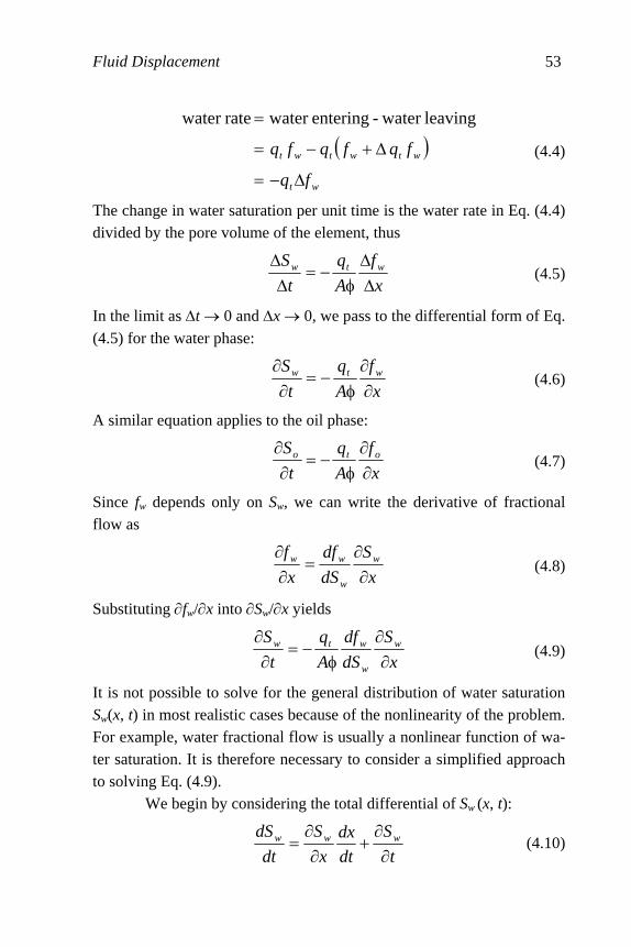
Fluid Displacement 53
( )wt
wtwtwt
fq
fqfqfq
∆−=
∆+−=
= leaving water - entering water ratewater
(4.4)
The change in water saturation per unit time is the water rate in Eq. (4.4) divided by the pore volume of the element, thus
x
f
A
q
t
S wtw
∆∆
φ−=
∆∆
(4.5)
In the limit as ∆t → 0 and ∆x → 0, we pass to the differential form of Eq. (4.5) for the water phase:
x
f
A
q
t
S wtw
∂∂
φ−=
∂∂
(4.6)
A similar equation applies to the oil phase:
x
f
A
q
t
S oto
∂∂
φ−=
∂∂
(4.7)
Since fw depends only on Sw, we can write the derivative of fractional flow as
x
S
dS
df
x
f w
w
ww
∂∂
=∂∂
(4.8)
Substituting ∂fw/∂x into ∂Sw/∂x yields
x
S
dS
df
A
q
t
S w
w
wtw
∂∂
φ−=
∂∂
(4.9)
It is not possible to solve for the general distribution of water saturation Sw(x, t) in most realistic cases because of the nonlinearity of the problem. For example, water fractional flow is usually a nonlinear function of wa-ter saturation. It is therefore necessary to consider a simplified approach to solving Eq. (4.9). We begin by considering the total differential of Sw (x, t):
t
S
dt
dx
x
S
dt
dS www
∂∂
+∂∂
= (4.10)

54 Principles of Applied Reservoir Simulation
Equation (4.10) can be simplified by choosing x to coincide with a sur-face of fixed Sw so that dSw/dt = 0 and
⎟⎠⎞
⎜⎝⎛∂∂
⎟⎠⎞
⎜⎝⎛∂∂
−=⎟⎠⎞
⎜⎝⎛
x
S
t
S
dt
dx
w
w
Sw
(4.11)
Substituting Eqs. (4.8) and (4.9) into Eq. (4.11) gives the Buckley-Leverett frontal advance equation:
ww Sw
wt
S dS
df
A
q
dt
dx⎟⎟⎠
⎞⎜⎜⎝
⎛φ
−=⎟⎠⎞
⎜⎝⎛
(4.12)
The derivative ( )wSdtdx is the velocity of the moving plane with water
saturation Sw, and the derivative ( )wSww dSdf is the slope of the frac-
tional flow curve. The integral of the frontal advance equation gives
w
w
Sw
wiS dS
df
A
Wx ⎟⎟
⎠
⎞⎜⎜⎝
⎛φ
= (4.13)
where
wSx distance traveled by a particular Sw contour (ft)
Wi cumulative water injected (cu ft)
( )wSww dSdf slope of fractional flow curve
4.1.1 Water Saturation Profile
A plot of Sw versus distance using Eq. (4.13) and typical frac-tional flow curves leads to the physically impossible situation of multiple values of Sw at a given location. A discontinuity in Sw at a cutoff location xc is needed to make the water saturation distribution single valued and to provide a material balance for wetting fluids. The procedure is sum-marized below.
Fluid Displacement 55
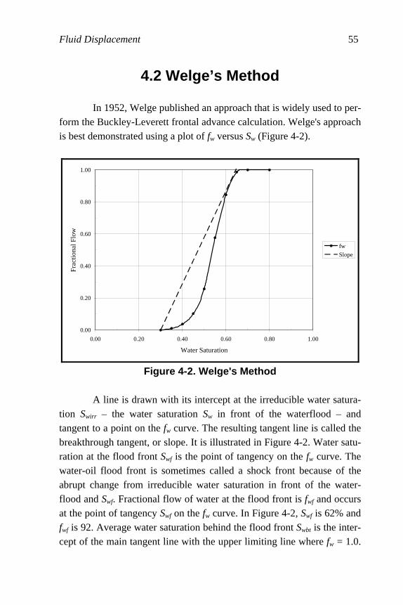
4.2 Welge’s Method In 1952, Welge published an approach that is widely used to per-form the Buckley-Leverett frontal advance calculation. Welge's approach is best demonstrated using a plot of fw versus Sw (Figure 4-2).
0.00
0.20
0.40
0.60
0.80
1.00
0.00 0.20 0.40 0.60 0.80 1.00
Water Saturation
Fra
ctio
nal
Flo
w
fw
Slope
Figure 4-2. Welge's Method
A line is drawn with its intercept at the irreducible water satura-tion Swirr – the water saturation Sw in front of the waterflood – and tangent to a point on the fw curve. The resulting tangent line is called the breakthrough tangent, or slope. It is illustrated in Figure 4-2. Water satu-ration at the flood front Swf is the point of tangency on the fw curve. The water-oil flood front is sometimes called a shock front because of the abrupt change from irreducible water saturation in front of the water-flood and Swf. Fractional flow of water at the flood front is fwf and occurs at the point of tangency Swf on the fw curve. In Figure 4-2, Swf is 62% and fwf is 92. Average water saturation behind the flood front Swbt is the inter-cept of the main tangent line with the upper limiting line where fw = 1.0.
56 Principles of Applied Reservoir Simulation
In Figure 4-2, average Swbt is 65%. In summary, when injected water reaches the producer, Welge’s approach gives the following results:
Ü Water saturation at the producing well is Swf Ü Average water saturation behind the front is Swbt Ü Producing water cut at reservoir conditions is fwf
Welge’s approach can be used to obtain other useful information
about the waterflood. The time to water breakthrough at the producer is
( )w
SwdS
wdfq
LAt
ibt
φ=
(4.14)
where
qi injection rate
( )wSww dSdf slope of main tangent line
L linear distance from injection well to production well
Cumulative water injected is given by
( )wfSww
i dSdfQ
1= (4.15)
where Qi is the cumulative pore volume of injected water. The slope of
the water fractional flow curve with respect to water saturation ww dSdf
evaluated at the water saturation at breakthrough wbtS gives cumulative
water injection Qi at breakthrough.
4.2.1 Effects of Capillary Pressure and Gravity In the absence of capillary pressure and gravity effects, the flood front propagates as a relatively "sharp" step function, or piston-like dis-placement. The example in Section 4.5 shows that the characterization of the front as sharp or piston-like is only approximate. In an ideal piston displacement, only one phase would flow on either side of the front.
Fluid Displacement 57
The presence of capillary pressure leads to the imbibition of wa-ter ahead of the front. This causes a change in the behavior of produced fluid ratios. Rather than an abrupt increase in water-oil ratio (WOR) as-sociated with piston-like displacement, the WOR will increase gradually as the leading edge of the mobile water reaches the well and is produced. In addition, the WOR will begin to increase sooner than it would have in the absence of capillary pressure. By contrast, gravity causes high Sw values to lag behind the front. The result is a smeared or "dispersed" flood front.
4.3 Miscible Displacement Buckley-Leverett theory treats the displacement of one fluid by another under immiscible, piston-like conditions. An immiscible dis-placement occurs when the displaced fluid and the displacing fluid do not mix. The result is a readily discernible interface between the two flu-ids. In a miscible displacement, the displaced and displacing fluids mix and the interfacial tension between the fluids approaches zero at their interface. A miscible displacement system can be modeled by a convec-tion-dispersion (C-D) equation. As an illustration, consider the one-dimensional C-D equation for the concentration C of the displacing fluid:
t
C
x
Cv
x
CD
∂∂
=∂∂
−∂∂
2
2
(4.16)
We assume here that dispersion D and velocity v are real, scalar con-
stants. The diffusion term has the Fickian form D⋅∂2C/∂x2 and the
convection term is v⋅∂C/∂x. When the diffusion term is much larger than the convection term, the C-D equation behaves like the heat conduction equation, which is a parabolic partial differential equation (PDE). If the diffusion term is much smaller than the convection term, the C-D equa-tion behaves like a first-order hyperbolic PDE. The C-D equation is especially valuable for studying numerical solutions of fluid flow equations because the C-D equation can be solved analytically and the C-D equation may be used to examine two important
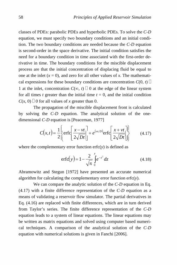
58 Principles of Applied Reservoir Simulation
classes of PDEs: parabolic PDEs and hyperbolic PDEs. To solve the C-D equation, we must specify two boundary conditions and an initial condi-tion. The two boundary conditions are needed because the C-D equation is second-order in the space derivative. The initial condition satisfies the need for a boundary condition in time associated with the first-order de-rivative in time. The boundary conditions for the miscible displacement process are that the initial concentration of displacing fluid be equal to one at the inlet (x = 0), and zero for all other values of x. The mathemati-
cal expressions for these boundary conditions are concentration C(0, t)
1 at the inlet, concentration C(∞, t) 0 at the edge of the linear system for all times t greater than the initial time t = 0, and the initial condition
C(x, 0) 0 for all values of x greater than 0. The propagation of the miscible displacement front is calculated by solving the C-D equation. The analytical solution of the one-dimensional C-D equation is [Peaceman, 1977]
( ) ( )
⎪⎭
⎪⎬⎫
⎪⎩
⎪⎨⎧
⎥⎥⎦
⎤
⎢⎢⎣
⎡ ++
⎥⎥⎦
⎤
⎢⎢⎣
⎡ −=
Dt
vtxe
Dt
vtxtxC Dvx
2erfc
2erfc
2
1, (4.17)
where the complementary error function erfc(y) is defined as
( ) ∫ −
π−=
y
z dzey0
221erfc (4.18)
Abramowitz and Stegun [1972] have presented an accurate numerical algorithm for calculating the complementary error function erfc(y).
We can compare the analytic solution of the C-D equation in Eq. (4.17) with a finite difference representation of the C-D equation as a means of validating a reservoir flow simulator. The partial derivatives in Eq. (4.16) are replaced with finite differences, which are in turn derived from Taylor’s series. The finite difference representation of the C-D equation leads to a system of linear equations. The linear equations may be written as matrix equations and solved using computer based numeri-cal techniques. A comparison of the analytical solution of the C-D equation with numerical solutions is given in Fanchi [2006].

Fluid Displacement 59
4.4 Viscous Fingering Viscous fingering is the unstable displacement of a more viscous fluid by a less viscous fluid. The fingering of an injection fluid into an in
situ fluid can influence reservoir flow behavior and adversely impact recovery. It is important to note, however, that fingering occurs even in the absence of a porous medium. If a low viscosity fluid is injected into a cell containing a high viscosity fluid, the low viscosity fluid will begin to form fingers as it moves through the fluid. It will not uniformly displace the higher viscosity fluid. These fingers can have different shapes. Figure 4-3 shows an example of a “skeletal” finger [Daccord, et al., 1986] while Figure 4-4 illustrates “fleshy” fingers [for example, see Paterson, 1985; Fanchi and Christiansen, 1989]. If we watch fingers evolve in a homoge-neous medium (Figure4-4), we see fingering display a symmetric pattern. The symmetry can be lost if there is some heterogeneity in the system.
Figure 4-3. "Skeletal" Viscous Finger (after Daccord, et al. [1986]; reprinted by permission of the American Physical
Society) Fingering can be a reservoir heterogeneity problem or a fluid displacement problem. Most reservoir simulators do not accurately model fingering effects. It is possible to improve model accuracy by us-ing a very fine grid to cover the area of interest, but the benefits

60 Principles of Applied Reservoir Simulation
associated with such a fine grid are seldom sufficient to justify the addi-tional cost.
a. b.
c. d.
Figure 4-4. Fleshy Viscous Finger Growth (Fanchi and Christiansen [1989]; reprinted by permission of the Society of
Petroleum Engineers)
4.5 IFLO Application: Buckley-Leverett Displacement
Flow models can be used to approximate Buckley-Leverett dis-placement. Figure 4-5 illustrates flow through a core and the corresponding flow model representation. A similar flow model can be used to approximate linear flow between an injection well and a produc-tion well in the field. Buckley-Leverett displacement is approximated in a flow model by making comparable assumptions. For example, fluid properties should be constant, the fluids should be treated as incom-pressible, and the displacement should be immiscible.

Fluid Displacement 61
gridblocks
coreinject produce
Figure 4-5. Modeling Linear Displacement
Figure 4-6 is a plot of water saturation versus gridblock number
at 180 and 366 days for water displacing oil in a linear, horizontal dis-placement. Water is injected in gridblock 1 and oil is produced from gridblock 20. The water-oil front is moving from left to right. The front is represented by the increase in water saturation from irreducible water saturation ahead of the front. In this case, irreducible water saturation is 20%. Residual oil saturation in this example is also 20%.
0
0.1
0.2
0.3
0.4
0.5
0.6
0.7
0.8
0.9
0 2 4 6 8 10 12 14 16 18 20
x-direction index (I)
Wat
er S
atu
ratio
n (f
ract
ion
)
180 days 366 days
Figure 4-6. Frontal Advance in Linear Displacement
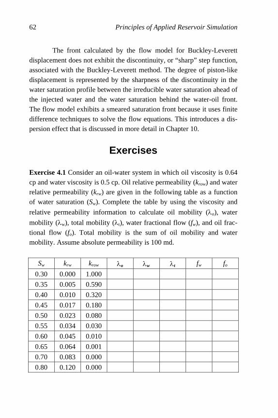
62 Principles of Applied Reservoir Simulation
The front calculated by the flow model for Buckley-Leverett displacement does not exhibit the discontinuity, or “sharp” step function, associated with the Buckley-Leverett method. The degree of piston-like displacement is represented by the sharpness of the discontinuity in the water saturation profile between the irreducible water saturation ahead of the injected water and the water saturation behind the water-oil front. The flow model exhibits a smeared saturation front because it uses finite difference techniques to solve the flow equations. This introduces a dis-persion effect that is discussed in more detail in Chapter 10.
Exercises
Exercise 4.1 Consider an oil-water system in which oil viscosity is 0.64 cp and water viscosity is 0.5 cp. Oil relative permeability (krow) and water relative permeability (krw) are given in the following table as a function of water saturation (Sw). Complete the table by using the viscosity and
relative permeability information to calculate oil mobility (λo), water
mobility (λw), total mobility (λt), water fractional flow (fw), and oil frac-
tional flow (fo). Total mobility is the sum of oil mobility and water mobility. Assume absolute permeability is 100 md.
Sw krw krow λo λw λt fw fo
0.30 0.000 1.000
0.35 0.005 0.590
0.40 0.010 0.320
0.45 0.017 0.180
0.50 0.023 0.080
0.55 0.034 0.030
0.60 0.045 0.010
0.65 0.064 0.001
0.70 0.083 0.000
0.80 0.120 0.000

Fluid Displacement 63
Exercise 4.2 Plot λo, λw, and λt in Exercise 4.1 as a function of Sw. What
is the mobility ratio of the oil-water system? Hint: see Eq. (3.14). Exercise 4.3 Plot fo and fw in Exercise 4.1 as a function of Sw. Use the plot of fw versus Sw and Welge’s method to determine water saturation at the producing well, average water saturation behind the front, and pro-ducing water cut at reservoir conditions. Exercise 4.4 Run EXAM3.DAT and plot water saturation as a function of distance between wells at 180 and 366 days. Hint: water saturation is reported in the run output file ITEMP.ROF. Exercise 4.5A Buckley-Leverett displacement through a linear, horizon-tal fracture with a matrix rock undergoing water imbibition can be modeled by the equation
( ) εε∂
∂
φλ
+∂∂
=∂
∂− ∫ ε−λ−∞ d
Se
R
t
S
x
fu
twft
f
wwf
0
where:
u = qt/Aφf = interstitial velocity (ft/day)
fwf = fractional flow of water in fracture
Swf = water saturation in fracture (fraction)
φf = fracture porosity (fraction)
ε = dummy integration variable (days)
∞R = asymptotic limit of oil recovery from the matrix into the fracture
λ = rate of convergence toward the asymptotic limit (day-1)
The integral term in the equation represents the matrix-fracture interac-tion, i.e. fluid flow between the matrix and the fracture. Is there flow
between the matrix and fracture if λ or ∞R is zero?
Exercise 4.5B Does the water imbibition rate from the fracture increase
or decrease when λ increases in the range 0 day-1 ≤ λ ≤ 1 day-1?

64 Principles of Applied Reservoir Simulation
Exercise 4.6 Plot the concentration C(x, t) in Eq. (4.17) given the follow-ing physical parameters: D = 0.1 ft2/day, v = 1 ft/day. The plot should
present C(x, t) in the range 0 ≤ x ≤ 1 for the three times t = 0.1 day, 0.2 day, 0.3 day. This data represents fluid movement in porous media, such as water draining through sand on a beach.

65
Chapter 5
Frontal Stability The stability of a flood front can influence the efficiency of fluid displacement. A front is stable if it retains the shape of the interface be-tween displaced and displacing fluids as the front moves through the medium. An analysis of frontal stability is presented in this chapter in terms of a specific example – the advance of a water-oil displacement front. The stability of the front is considered both in the absence of grav-ity and in the presence of gravity. Front stability is then studied using linear stability analysis.
5.1 Frontal Advance Neglecting Gravity The displacement of one phase by another may be analytically studied if we simplify the problem to displacement in a linear, homoge-nous porous medium. Let us first consider the displacement of oil by water in a horizontal porous medium of length L. We assume piston-like displacement of a front located at xf. Application of Darcy’s Law and the continuity equation leads to a pressure distribution described by Pois-son’s equation. The absence of sources or sinks in the medium reduces Poisson’s equation to the Laplace equation for the water phase pressure:
fw xx
x
P<<=
∂∂
0,02
2
(5.1)
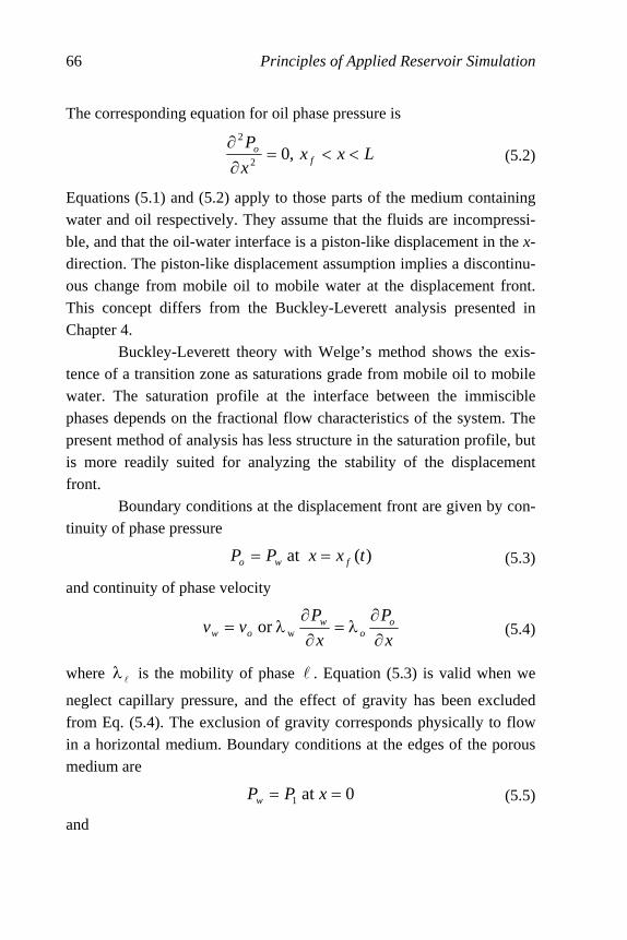
66 Principles of Applied Reservoir Simulation
The corresponding equation for oil phase pressure is
Lxxx
Pf
o <<=∂∂
,02
2
(5.2)
Equations (5.1) and (5.2) apply to those parts of the medium containing water and oil respectively. They assume that the fluids are incompressi-ble, and that the oil-water interface is a piston-like displacement in the x-direction. The piston-like displacement assumption implies a discontinu-ous change from mobile oil to mobile water at the displacement front. This concept differs from the Buckley-Leverett analysis presented in Chapter 4.
Buckley-Leverett theory with Welge’s method shows the exis-tence of a transition zone as saturations grade from mobile oil to mobile water. The saturation profile at the interface between the immiscible phases depends on the fractional flow characteristics of the system. The present method of analysis has less structure in the saturation profile, but is more readily suited for analyzing the stability of the displacement front. Boundary conditions at the displacement front are given by con-tinuity of phase pressure
)(at txxPP fwo == (5.3)
and continuity of phase velocity
x
P
x
Pvv o
ow
ow ∂∂
λ=∂∂
λ= wor (5.4)
where lλ is the mobility of phase l . Equation (5.3) is valid when we
neglect capillary pressure, and the effect of gravity has been excluded from Eq. (5.4). The exclusion of gravity corresponds physically to flow in a horizontal medium. Boundary conditions at the edges of the porous medium are
0at 1 == xPPw (5.5)
and

Frontal Stability
67
LxPPo == at 2 (5.6)
Equations (5.1) through (5.6) may be solved analytically. We begin by integrating Eqs. (5.1) and (5.2) to find the general solutions
www BxAP += (5.7)
and
ooo BxAP += (5.8)
where the constant coefficients { }ll BA , are determined by applying the
boundary conditions. Substituting Eq. (5.5) into Eq. (5.7) gives
1PBw = (5.9)
The remaining coefficients are found by simultaneously solving Eqs. (5.4), (5.7), and (5.8) subject to Eqs. (5.3), (5.5), and (5.6). The resulting coefficients are
f
w xMML
PA
)1( −+∆
−= (5.10)
wo AMA = (5.11)
fwfowo xAMPxAAPB )1()( 11 −+=−== (5.12)
where M is the mobility ratio
o
wMλλ
= (5.13)
and the pressure difference is
21 PPP −=∆ (5.14)
The frontal velocity vf is given by
( )wcor
wff SS
v
dt
dxv
−−φ=≡
1 (5.15)
where Sor is residual oil saturation, Swc is connate water saturation, and vw is the Darcy velocity given by Darcy’s Law without gravity effects in one spatial dimension, namely:

68 Principles of Applied Reservoir Simulation
www
ww Ax
Pv λ−=
∂∂
λ−= (5.16)
Substituting Eq. (5.16) into (5.15) gives
[ ]fwcor
wf
xMMLSS
P
td
xd
)1(
1
)1( −+−−φ∆λ
= (5.17)
The integral of Eq. (5.17) with respect to time gives the frontal advance.
5.2 Frontal Advance Including Gravity Gravity is included in the analysis of frontal advance in a dip-ping reservoir (Figure 5-1) by replacing phase pressure in Eqs. (5.1) through (5.6) with phase potential
Θρ−=Φ sinxgP lll
2Φ
1Φ Θ
fx
Figure 5-1. Geometry of Frontal Advance
The resulting equations for phase potentials are
fw xx
x<<=
∂Φ∂
0,02
2
(5.18)
Lxxx f
o <<=∂Φ∂
,02
2
(5.19)
The phase potentials at the flood front are related by

Frontal Stability
69
Θρ−ρ+Φ=Φ sin)( fwowo gx (5.20)
with continuity of phase velocities
xx
oo
ww ∂
Φ∂λ=
∂Φ∂
λ (5.21)
The boundary conditions for the phase potentials are
0at 1 =Φ=Φ xw (5.22)
and
Lxo =Φ=Φ at 2 (5.23)
Capillary pressure is still neglected in this formulation. Equation (5.20) is the analog of Eq. (5.3).
The solutions of the second-order ordinary differential equations given by Eqs. (5.18) and (5.19) are the linear relationships
www BxA ′+′=Φ (5.24)
ooo BxA ′+′=Φ (5.25)
The coefficients are evaluated by substituting Eqs. (5.24) and (5.25) into Eqs. (5.18) and (5.19) and applying the boundary conditions. The coeffi-cients are
⎥⎥⎦
⎤
⎢⎢⎣
⎡
−+
Θρ−ρ+Φ−Φ−=′
f
wofw xMML
gxA
)1(
sin)()( 21(5.26)
wo AMA ′=′ (5.27)
1Φ=′wB (5.28)
LAMLAB woo ′−Φ=′−Φ=′ 22 (5.29)
The Darcy velocity of the water phase is
www
ww Ax
v ′λ−=∂Φ∂
λ−= (5.30)
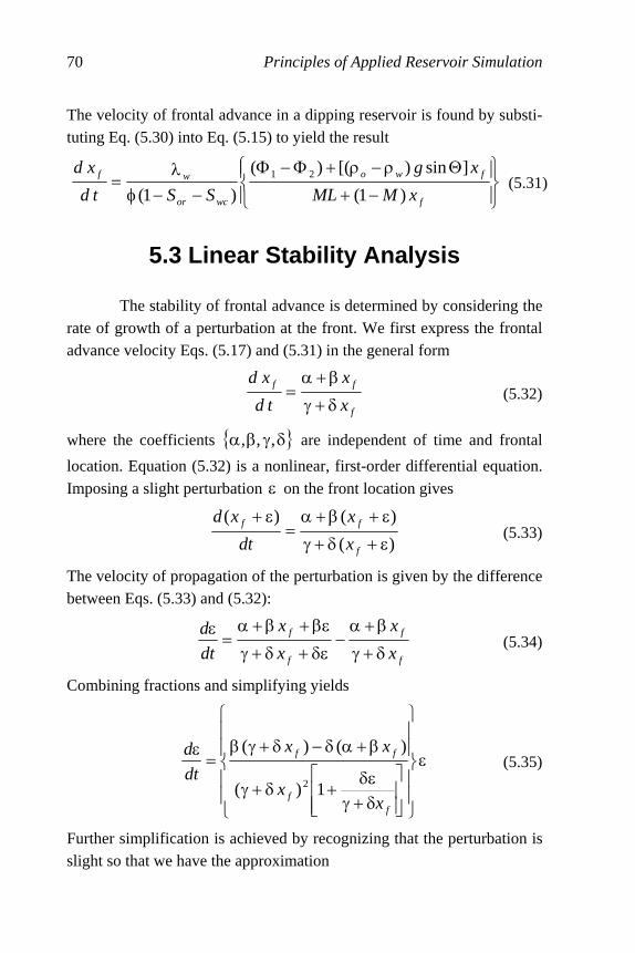
70 Principles of Applied Reservoir Simulation
The velocity of frontal advance in a dipping reservoir is found by substi-tuting Eq. (5.30) into Eq. (5.15) to yield the result
⎪⎭
⎪⎬⎫
⎪⎩
⎪⎨⎧
−+
Θρ−ρ+Φ−Φ
−−φλ
=f
fwo
wcor
wf
xMML
xg
SStd
xd
)1(
]sin)[()(
)1(21
(5.31)
5.3 Linear Stability Analysis The stability of frontal advance is determined by considering the rate of growth of a perturbation at the front. We first express the frontal advance velocity Eqs. (5.17) and (5.31) in the general form
f
ff
x
x
td
xd
δ+γ
β+α= (5.32)
where the coefficients { }δγβα ,,, are independent of time and frontal
location. Equation (5.32) is a nonlinear, first-order differential equation. Imposing a slight perturbation ε on the front location gives
)(
)()(
ε+δ+γ
ε+β+α=
ε+
f
ff
x
x
dt
xd (5.33)
The velocity of propagation of the perturbation is given by the difference between Eqs. (5.33) and (5.32):
f
f
f
f
x
x
x
x
dt
d
δ+γ
β+α−
δε+δ+γ
βε+β+α=
ε (5.34)
Combining fractions and simplifying yields
ε
⎪⎪
⎭
⎪⎪
⎬
⎫
⎪⎪
⎩
⎪⎪
⎨
⎧
⎥⎥⎦
⎤
⎢⎢⎣
⎡
δ+γδε
+δ+γ
β+αδ−δ+γβ=
ε
ff
ff
xx
xx
dt
d
1)(
)()(
2
(5.35)
Further simplification is achieved by recognizing that the perturbation is slight so that we have the approximation
Frontal Stability
71
f
f
f
xx
x
δ+γ<<δεδ+γδε
−≈
δ+γδε
+for1
1
1
(5.36)
Substituting Eq. (5.36) into Eq. (5.35) gives
⎥⎥⎦
⎤
⎢⎢⎣
⎡
δ+γδε
−⎪⎭
⎪⎬⎫
⎪⎩
⎪⎨⎧
δ+γ
β+αδ−δ+γβ=
ε
ff
ff
xx
xx
dt
d1
)(
)()(2 (5.37)
Keeping only terms to first order in g and simplifying gives
2)(
)(
fxdt
d
δ+γεδα−βγ
=ε
(5.38)
Equation (5.38) has the solution
τε=ε te0 (5.39)
where ε0 is an integration constant, and
2)( fxδ+γδα−βγ
=τ (5.40)
If τ is negative, the perturbation decays exponentially. If τ is greater than
zero, the perturbation grows exponentially. Finally, if τ equals zero, the
perturbation does not propagate because dε/dt = 0 in Eq. (5.38).
We can now examine the stability of a displacement front. Com-paring Eq. (5.32) with (5.31) lets us make the identifications
)1(
)( 21
wcor
w
SS −−φΦ−Φλ
=α (5.41)
)1(
sin)(
wcor
wow
SS
g
−−φΘρ−ρλ
=β (5.42)
LM=γ (5.43)
)1( M−=δ (5.44)
The resulting expression for the growth of a perturbation is
72 Principles of Applied Reservoir Simulation
[ ] 221
)1(
sin)()()1(
)1(
f
wo
wcor
w
xMML
gMLM
SSdt
d
−+Θρ−ρ+Φ−Φ−
×
−−φελ
−=ε
(5.45)
Equation (5.45) agrees with Eq. (7-104) in Collins [1961]. Zero growth rate of a perturbation is determined by setting the
derivative dε/dt = 0 in Eq. (5.45). The resulting condition for zero
growth rate is
0sin)()()1( 21 =Θρ−ρ+Φ−Φ− gMLM wo (5.46)
If the medium is horizontal, the condition for a system without gravity is
0)1( =∆− PM (5.47)
To see the effect of mobility ratio M on finger growth for the gravity-free case, we set g = 0 in Eq. (5.45) to get
2])1([
)1(
)1( fwcor
w
xMML
PM
SSdt
d
−+∆−
−−φελ
−=ε
(5.48)
The finger grows exponentially if M > 1, decays exponentially if M < 1, and does not propagate if M = 1.
5.4 IFLO Application: Frontal Advance in a Dipping Reservoir
The effect of mobility and gravity on frontal advance can be studied using a flow model of an oil reservoir waterflood. We consider a linear waterflood that has constant oil viscosity and constant water vis-cosity. Table 5-1 shows the four cases of interest. The cases differ by dip angle or oil viscosity. Each of these effects is considered separately. Figure 5-2 shows the effect of gravity on water saturation pro-files for Cases A and B. The figure is a plot of water saturation versus gridblock number. Water is injected in gridblock #1 and oil is produced from gridblock #20. Cases A and B are the same except for dip angle.

Frontal Stability
73
The effect of gravity is to make the frontal advance a bit more piston-like, but the effect is relatively minor for Cases A and B. The front in Figure 5-2 is represented by the increase in water saturation between blocks 14 and 16.
Table 5-1 Frontal Advance Cases
CaseDip Angle(degrees)
Oil Viscosity(cp)
Mobility Ratio
A 0 2 1.56
B 25 2 1.56
C 25 5 3.89
D 25 1 0.78
0.0
0.1
0.2
0.3
0.4
0.5
0.6
0.7
0.8
0.9
0 2 4 6 8 10 12 14 16 18 20
Block #
Wat
er S
atu
ratio
n (f
ract
ion
)
Dip = 0 degrees Dip = 25 degrees
Figure 5-2. Effect of Dip Angle on Frontal Advance
Figure 5-3 shows the effect of mobility ratio on frontal advance. Cases B, C and D differ only by oil viscosity, which represents a differ-ence in mobility ratio. The mobility ratio of Case D is less than one, which is considered favorable. The mobility ratios of Cases B and C are larger than one and are, therefore, considered unfavorable. Case D with a

74 Principles of Applied Reservoir Simulation
favorable mobility ratio has a more piston-like displacement than either Case B or C. The front is less piston-like as mobility ratio increases. The water saturation profile for Case C shows that water breakthrough has occurred at the production well. This is verified by plotting water pro-duction rate as a function of time in Figure 5-4.
0.0
0.1
0.2
0.3
0.4
0.5
0.6
0.7
0.8
0.9
0 2 4 6 8 10 12 14 16 18 20
Block #
Wat
er S
atur
atio
n (
frac
tion)
Oil Vis = 1 cp Oil Vis = 2 cp Oil Vis = 5 cp
Figure 5-3. Effect of Mobility Ratio on Frontal Advance
0
10
20
30
40
50
60
70
80
0 50 100 150 200 250 300 350 400
Time (days)
Wat
er P
rod
Rat
e (
ST
B/D
)
Oil Vis = 2 cp Oil Vis = 5 cp
Figure 5-4. Water Production Rate for Cases B and C
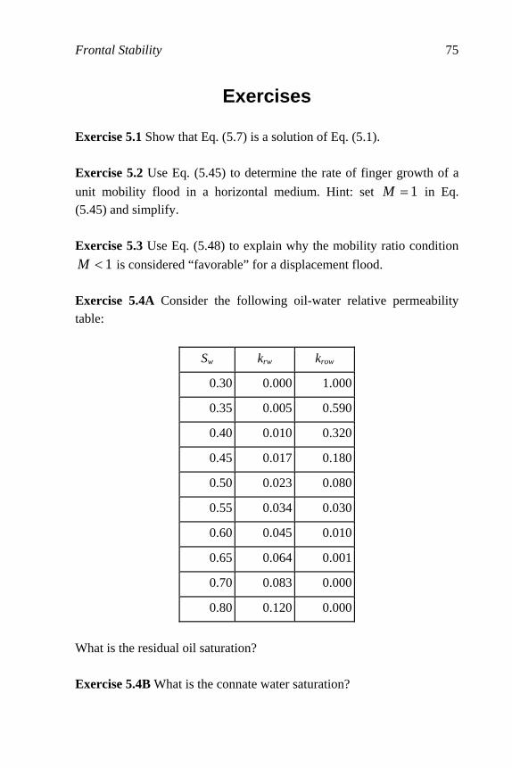
Frontal Stability
75
Exercises
Exercise 5.1 Show that Eq. (5.7) is a solution of Eq. (5.1). Exercise 5.2 Use Eq. (5.45) to determine the rate of finger growth of a
unit mobility flood in a horizontal medium. Hint: set 1=M in Eq. (5.45) and simplify. Exercise 5.3 Use Eq. (5.48) to explain why the mobility ratio condition
1<M is considered “favorable” for a displacement flood. Exercise 5.4A Consider the following oil-water relative permeability table:
Sw krw krow
0.30 0.000 1.000
0.35 0.005 0.590
0.40 0.010 0.320
0.45 0.017 0.180
0.50 0.023 0.080
0.55 0.034 0.030
0.60 0.045 0.010
0.65 0.064 0.001
0.70 0.083 0.000
0.80 0.120 0.000
What is the residual oil saturation? Exercise 5.4B What is the connate water saturation?
76 Principles of Applied Reservoir Simulation
Exercise 5.4C What is the relative permeability to oil at connate water saturation for the oil-water relative permeability curves? Exercise 5.4D What is the relative permeability to water at residual oil saturation? Exercise 5.4E Assume oil viscosity is 0.64 cp and water viscosity is 0.50 cp. Calculate the mobility ratio of a waterflood for water displacing oil using the oil-water relative permeability curves above. Exercise 5.4F Is the mobility ratio favorable or unfavorable? Exercise 5.5A Consider a linear flow system with area = 25 ft2 and per-meability = 100 md. End point A is 5 ft higher than end point B, and the distance between end points is 15 ft. Suppose the system contains oil with viscosity = 0.8 cp, gravity = 35o API (けo = 0.85), and FVF = 1.0 RB/STB. If the end point pressures are PA = PB = 20 psia, is there flow? If so, how much and in what direction? Use Darcy’s Law
⎥⎦
⎤⎢⎣
⎡αρ+
−βµ
−= sin001127.0 gL
PPAkq BA
with the gravity term and dip angle g. Exercise 5.5B What should the pressure PB be to prevent fluid flow? Exercise 5.6A Files EXAM3A.DAT and EXAM3B.DAT model a linear
waterflood in a formation with a dip angle of 25°. The oil viscosity is 2 cp in EXAM3A.DAT and 5 cp in EXAM3B.DAT. Run both data files and plot water production rate versus time using data from timestep summary file ITEMP.TSS. Exercise 5.6B Run data files EXAM3A.DAT and EXAM3B.DAT. Plot water saturation at the end of the run versus gridblock number using data

Frontal Stability
77
from run output file ITEMP.ROF. There are twenty gridblocks in the x-direction. Exercise 5.6C Explain the differences between the results in Parts A and B of this exercise.

78
Chapter 6
Pattern Floods
The effectiveness of a displacement process depends on many factors, including reservoir and fluid characteristics that are beyond our control, such as depth, structure, and fluid type. Other factors that influ-ence displacement efficiency can be controlled, however. They include the number and type of wells, well rates, and well locations. The distri-bution of wells is known as the well pattern. The impact of well pattern on displacement effectiveness is discussed after definitions of recovery efficiency are presented. The selection of a development plan depends on a comparison of the economics of alternative development concepts. Reservoir flow models are especially useful tools for performing these studies.
6.1 Recovery Efficiency Recovery efficiency is quantified by comparing initial and final volumes of fluid in place. It takes into account volumetric and displace-ment efficiencies. The different aspects of recovery efficiency are defined and then combined to form overall recovery efficiency. Displacement efficiency accounts for the efficiency of recover-ing mobile hydrocarbon. To be specific, we define displacement efficiency for oil as the ratio of mobile oil to original oil in place at res-ervoir conditions:
Pattern Floods 79
oi
oroi
oip
orpoipD S
SS
SV
SVSVE
−=
−= (6.1)
where
Vp initial pore volume
Soi initial oil saturation
Sor residual oil saturation
Residual oil saturation is replaced by oil saturation at abandonment in floods that do not reduce initial oil saturation to residual oil saturation during the life of the flood. Displacement efficiency can approach 100% if residual oil saturation can be driven to zero. One of the goals of en-hanced oil recovery processes such as micellar-polymer flooding or miscible flooding is to reduce residual oil saturation and increase dis-placement efficiency. The definition of displacement efficiency can be modified to include the effects of swelling. Swelling is represented by using surface volume rather than reservoir volume in the definition of displacement efficiency. The volume conversion is achieved by dividing reservoir vol-ume by formation volume factor (FVF). For example, the displacement efficiency of a waterflood is
oi
oi
oa
or
oi
oi
oi
oip
oa
orp
oi
oip
D
B
SB
S
B
S
B
SVB
SV
B
SV
E
−=
−= (6.2)
where
Boi oil FVF at the beginning of waterflood
Boa oil FVF at the waterflood pressure
Notice that oil formation volume factor is at its maximum value at the bubble point pressure of the oil. If the waterflood is conducted at or just above the bubble point pressure, the value of Boa will be maximized and
80 Principles of Applied Reservoir Simulation
the residual oil term will be minimized. The resulting displacement effi-ciency for a waterflood is then maximized. Displacement efficiency is a measure of how effectively mobile hydrocarbons can be recovered. Although the above definitions of dis-placement efficiency have been given for oil, similar definitions can be provided for gas. In addition to displacement efficiency, volumetric factors are needed to determine overall recovery efficiency. Areal and vertical sweep efficiencies are defined by
areatotal
areaswept=AE (6.3)
and
thicknesstotal
thicknessswept=VE (6.4)
Reservoir flow models are useful tools for quantifying both swept area and swept thickness. Vertical sweep efficiency depends on the vertical distribution of the flow capacity of each formation intersected by the wellbore, where flow capacity is the product of permeability and net thickness. The flow capacity of a model layer should honor observed reservoir flow capacity, especially if high flow capacity thief zones are present. The product of areal and vertical sweep efficiency is the volu-metric sweep efficiency Evol:
VAvol EEE ×= (6.5)
where
EA areal sweep efficiency
EV vertical sweep efficiency
Overall recovery efficiency must account for both volumetric and displacement effects. It is therefore defined as the product of volu-metric sweep efficiency and displacement efficiency:
VADvolD EEEEERE ××=×= (6.6)
where

Pattern Floods 81
RE recovery efficiency
Notice that each of the efficiency factors in recovery efficiency can be relatively large, and yet recovery efficiency will be relatively small. For example, suppose both the areal and vertical efficiencies are 70% and displacement efficiency is 80%, the product of these efficiencies is ap-proximately 39%. This means that even the reservoirs with the best recovery efficiency often have a substantial volume of unrecovered hy-drocarbon remaining in the ground. The most important goal of improved recovery techniques is the recovery of this remaining resource.
6.2 Patterns and Spacing The analytical techniques for describing displacement that were discussed previously study fluid displacement between one injection well and one production well. The alignment of the injector-producer pair represents a linear displacement process. It is the simplest pattern involv-ing injection and production wells. A variety of other patterns may be defined. Several examples are shown in Figure 6-1. A representative pattern element for the five-spot pattern is identified using shaded wells.
The ratio of the number of producing wells to the number of in-jection wells is shown in Table 6-1. The patterns depicted in Table 6-1 and Figure 6-1 are symmetric patterns that are especially effective for reservoirs with relatively small dip and large areal extent. The injectors and producers are generally interspersed. Other patterns in which injec-tors and producers are grouped together may be needed for reservoirs with significant dip. For example, a peripheral or flank injection pattern may be needed to effectively flood an anticlinal or monoclinal reservoir.

82 Principles of Applied Reservoir Simulation
• • • • • ◊ à à à à • • • • • à à à à à • • • • •
Direct Line-Drive Pattern a = distance between neighboring wells
d = distance between rows of wells
• denotes production well
◊伊 denotes injection well
• • • • • à à à à à à • • • • • à à à à à à • • • • •
Staggered Line-Drive Pattern a = distance between neighboring wells
d = distance between rows of wells
• denotes production well
◊伊 denotes injection well
• à • à • à • à • à • à • à • à • à • à • à • à •
Five-Spot Pattern d = distance between neighboring
producers = distance between neighboring
injectors
• denotes production well
◊伊 denotes injection well
Figure 6-1. Well Locations in Selected Well Patterns

Pattern Floods 83
Table 6-1 Producer-to-Injector Ratios for Common Well Patterns
Well Pattern Producer : Injector Ratio
Four-Spot 2
Five-Spot 1
Direct Line-drive 1
Staggered Line-drive 1
Seven-Spot 1 / 2
Nine-Spot 1 / 3
In addition to reservoir geometry and the displacement process, the well pattern depends on the distribution and orientation of existing production wells, and the desired spacing of wells. Wells may be ori-ented vertically, horizontally, or at some deviation angle between horizontal and vertical. The orientation of a well depends on such reser-voir features as formation orientation and, if fractures are present, fracture orientation. For example, if a reservoir contains many fractures that are oriented in a particular direction, recovery is often optimized by drilling a horizontal well in a direction that intersects as many fractures as possible. Recovery is optimized because recovery from fractured res-ervoirs usually occurs by producing fluid that flows from the matrix into the fractures and then to the wellbore.
Well spacing depends on the area being drained by a production well. A reduction in well spacing requires an increase in the density of production wells. The density of production wells is the number of pro-duction wells in a specified area. Well density can be increased by drilling additional wells in the space between wells in a process called infill drilling, which is discussed further in the next section.
84 Principles of Applied Reservoir Simulation
6.3 Advances in Drilling Technology
Improvements in drilling technology are having a dramatic im-pact on reservoir management. Longer wellbores that follow subsurface formations are providing access to more parts of the reservoir. The addi-tional information is being integrated into reservoir characterization at the same time that more detailed reservoir models are helping guide the longer wellbore trajectories. Four areas of drilling technology are briefly discussed here: infill drilling, multilateral wells, geosteering, and intelli-gent wells.
6.3.1 Infill Drilling
Infill drilling is a means of improving sweep efficiency by in-creasing the number of wells in an area. Well spacing is reduced to provide access to unswept parts of a field. Modifications to well patterns and the increase in well density can change sweep patterns and increase sweep efficiency, particularly in heterogeneous reservoirs. Infill drilling can improve recovery efficiency, but can also be more expensive than a fluid displacement process.
6.3.2 Multilateral Wells and Extended Reach Drilling Multilateral well technology is revolutionizing extraction tech-nology and reservoir management. A multilateral well is a well that has more than one flow conduit. Although the use of multilateral wells is considered a relatively recent development, Golan [2000] reported that the Russians had drilled a type of multilateral well in the Bashkiria Field as long ago as 1955. It had ten branches and its well schematic was pub-lished in the Russian literature and reported in Drilling Journal in December 1955 [page 87].

Pattern Floods 85
Multilateral wells were introduced into the modern industry as sidetracked wells that were drilled for the purpose of bypassing wells with casing problems. Today, multilateral wells make it possible to con-nect multiple well paths to a common wellbore. Figure 6-2 illustrates a multilateral well trajectory.
Reservoir Formation Cross-Section
HorizontalWell
BilateralWell
MultilateralWell
Figure 6-2. Example of a Multilateral Well
Multilateral wells have many applications. For example, they are useful in offshore environments where the number of well slots is sub-stantially limited by the amount of space available on a platform. They can also be used to produce highly compartmentalized reservoirs and reservoirs with low permeability. Extended reach horizontal or multilat-eral wells are useful in environmentally or commercially sensitive areas where placing a drilling rig is undesirable or prohibited.
6.3.3 Geosteering Geosteering is a technology for reaching drilling target locations and is a prerequisite for successful extended reach drilling. Extended reach drilling is used to drill a well with very long horizontal displace-ment away from the drilling rig. Extended reach drilling provides a means of reaching commercial subsurface deposits at great distances from a fixed drilling rig location. Three of the longest applications of extended reach drilling are at the Wytch Farm oil field offshore Britain, the Xijiang field in the South China Sea, and the Ara field offshore

86 Principles of Applied Reservoir Simulation
Tierra del Fuego, Argentina. These projects have drilled extended reach wells with approximately 8 km of horizontal displacement from the drill-ing rig. Geosteering and extended reach drilling have many benefits, including reducing costs associated with the construction of new plat-forms. Extended reach drilling lets an operator minimize the environmental footprint of a field development project.
6.3.4 Intelligent Wells It is often necessary in the management of a modern reservoir to alter the completion interval in a well. These adjustments are needed to modify producing well fluid ratios such as water-oil ratio or gas-oil ratio. One way to minimize the cost associated with completion interval ad-justments is to design a well that can change the completion interval automatically. This is an example of an intelligent well, which is also known as a “smart well.”
Intelligent wells are designed to give an operator remote control of subsurface well characteristics such as completion interval. In addi-tion, intelligent wells are being designed to provide information to the operator using downhole measurements of physical properties such as pressure, temperature and seismic vibrations. One goal of intelligent well technology is to convey a stream of continuous and real-time information to the operator who can monitor this information and make adjustments as needed to achieve reservoir management objectives.
6.4 Pattern Recovery Optimum performance may be achieved with the patterns de-fined in the previous section by controlling the rates of injectors and producers. These calculations can be performed analytically if we as-sume that the displacing and displaced fluids are incompressible, the mobility ratio is one, and the reservoir has uniform properties. Values of injection rates for the three patterns shown in Figure 6-1 are presented in Table 6-2 [Wilhite, 1986]. Units and nomenclature for the rate equations

Pattern Floods 87
in Table 6-2 are barrels per day for rate q; darcies for permeability k; feet for thickness h; well separations a and d, and wellbore radius rw; pounds
per square inch for pressure change ∆P; and centipoise for viscosity µ. The well separations are defined in Figure 6-1.
Table 6-2 Analytical Injection Rates for Selected Well Patterns
Pattern Rate
Direct Line-Drive 1,
838.1571.1ln
541.3≥
⎥⎦
⎤⎢⎣
⎡−+⎟⎟
⎠
⎞⎜⎜⎝
⎛µ
∆=
a
d
a
d
r
a
Pkhq
w
D
Staggered Line-Drive⎥⎦
⎤⎢⎣
⎡−+⎟⎟
⎠
⎞⎜⎜⎝
⎛µ
∆=
838.1571.1ln
541.3
a
d
r
a
Pkhq
w
S
Five-Spot ⎥⎦
⎤⎢⎣
⎡−⎟⎟
⎠
⎞⎜⎜⎝
⎛µ
∆=
619.0ln
541.3
w
F
r
a
Pkhq
The calculation of analytical injection rates, even under a set of restrictive assumptions, provides a methodology for designing well pat-terns without using a reservoir simulator. More accurate estimates of injection rates under a less restrictive set of assumptions are obtained using reservoir simulators. For example, simulators have been used to correlate volumetric sweep efficiency with mobility ratio and permeabil-ity variation in a reservoir that is being subjected to a pattern flood [Wilhite, 1986]. One measure of permeability variation is the Dykstra-Parsons coefficient of permeability variation. The Dykstra-Parsons coefficient can be estimated for a log-normal permeability distribution as
⎥⎦⎤
⎢⎣⎡−−= )(lnexp1
Hk
Ak
DPV
88 Principles of Applied Reservoir Simulation
where kA is the arithmetic average permeability for n samples
∑=
=n
iiA k
nk
1
1
and kH is the harmonic average permeability
∑=
=n
i iH knk 1
111
The Dykstra-Parsons coefficient should be in the range 0 ≤ VDP ≤ 1. For a perfectly homogeneous reservoir, VDP = 0 because kA = kH. An increase in reservoir heterogeneity increases VDP. Typical values of the Dykstra-
Parsons coefficient are in the range 0.4 ≤ VDP ≤ 0.9.
Correlations of volumetric sweep efficiency with mobility ratio and permeability variation show that volumetric sweep efficiency de-clines as reservoir heterogeneity increases or mobility ratio increases, particularly for mobility ratios greater than one. This makes sense physi-cally if we recall that mobility ratio is the mobility of the displacing fluid behind the front divided by the mobility of the displaced fluid ahead of the front. If the mobility of the displacing fluid is greater than the mobil-ity of the displaced fluid, then the mobility ratio is greater than one and is considered unfavorable. On the other hand, if the mobility of the dis-placing fluid is less than the mobility of the displaced fluid, then the mobility ratio is less than one and is considered favorable. Unfavorable mobility ratios often occur when gas displaces oil or when water dis-places high viscosity oil. An example of a flood with a favorable mobility ratio is the displacement of low viscosity oil by water.
6.5 IFLO Application: Five-Spot Waterflood
One of the most widely used patterns for waterflooding and gas-flooding is the five-spot pattern. We illustrate a pattern flood by considering the flood of the region shown in Figure 6-3. Well P-1 is an

Pattern Floods 89
oil production well that is surrounded by four injection wells. This model is similar to the example presented by Fanchi, et al. [1982].
P-1
I-1
I-2
I-3
I-4
Figure 6-3. Five-Spot Waterflood
The reservoir consists of two communicating layers. The flow capacity in the upper layer is less than the flow capacity in the lower layer, and the volume of oil in the upper layer is less than the volume of oil in the lower layer. Well P-1 drained the initially undersaturated reser-voir for one year prior to the onset of water injection. Bubble point pressure is 4014.7 psia. Primary depletion resulted in a substantial de-cline in reservoir pressure, the formation of a free gas phase, and a decline in oil production rate. Water injection was needed for pressure support and to sustain oil production rate.
Figure 6-4 and Figure 6-5 present reservoir pressure, oil produc-tion rate, and produced gas-oil ratio. Notice the change in the rate of reservoir pressure decline when reservoir pressure drops below bubble point pressure. The producing gas-oil ratio increases as a result of the formation of a free gas phase.
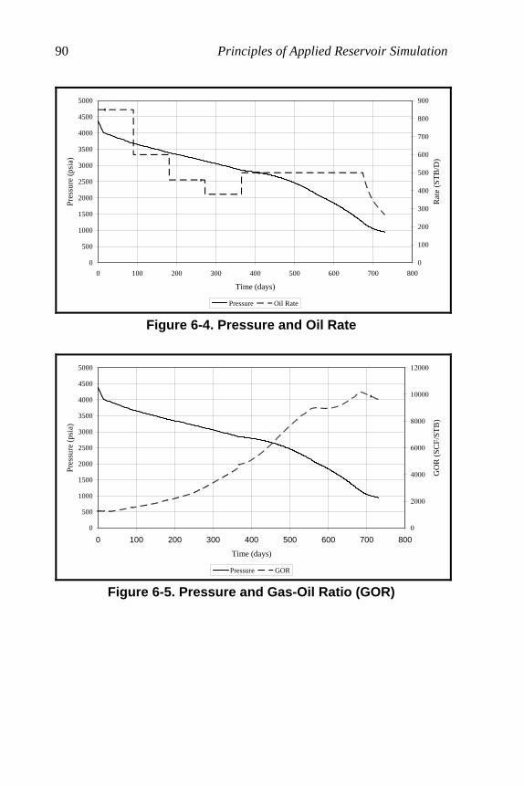
90 Principles of Applied Reservoir Simulation
0
500
1000
1500
2000
2500
3000
3500
4000
4500
5000
0 100 200 300 400 500 600 700 800
Time (days)
Pre
ssu
re (
psi
a)
0
100
200
300
400
500
600
700
800
900
Rat
e (S
TB
/D)
Pressure Oil Rate
Figure 6-4. Pressure and Oil Rate
0
500
1000
1500
2000
2500
3000
3500
4000
4500
5000
0 100 200 300 400 500 600 700 800
Time (days)
Pre
ssur
e (p
sia)
0
2000
4000
6000
8000
10000
12000
GO
R (
SC
F/S
TB
)
Pressure GOR
Figure 6-5. Pressure and Gas-Oil Ratio (GOR)
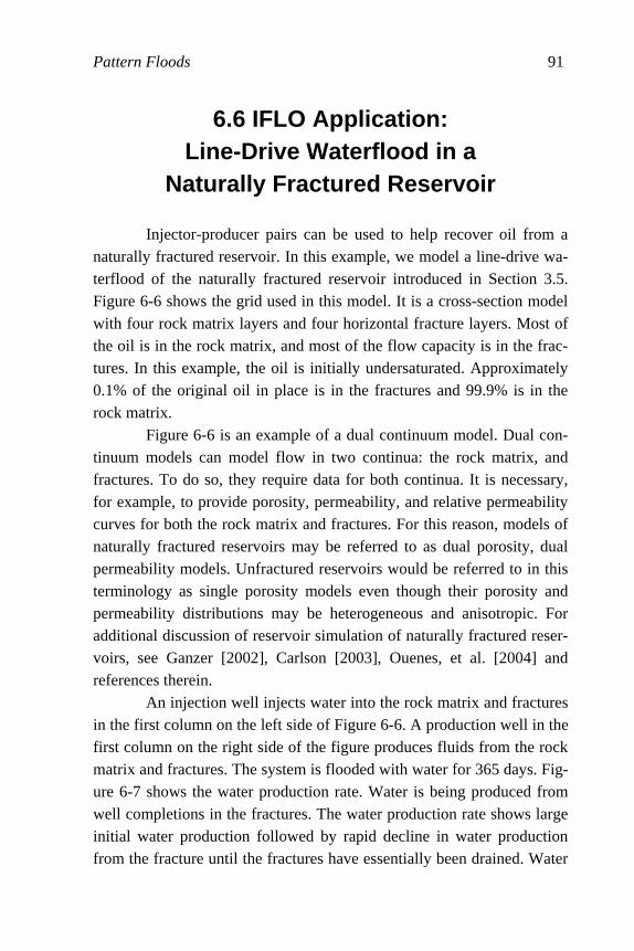
Pattern Floods 91
6.6 IFLO Application: Line-Drive Waterflood in a
Naturally Fractured Reservoir Injector-producer pairs can be used to help recover oil from a naturally fractured reservoir. In this example, we model a line-drive wa-terflood of the naturally fractured reservoir introduced in Section 3.5. Figure 6-6 shows the grid used in this model. It is a cross-section model with four rock matrix layers and four horizontal fracture layers. Most of the oil is in the rock matrix, and most of the flow capacity is in the frac-tures. In this example, the oil is initially undersaturated. Approximately 0.1% of the original oil in place is in the fractures and 99.9% is in the rock matrix.
Figure 6-6 is an example of a dual continuum model. Dual con-tinuum models can model flow in two continua: the rock matrix, and fractures. To do so, they require data for both continua. It is necessary, for example, to provide porosity, permeability, and relative permeability curves for both the rock matrix and fractures. For this reason, models of naturally fractured reservoirs may be referred to as dual porosity, dual permeability models. Unfractured reservoirs would be referred to in this terminology as single porosity models even though their porosity and permeability distributions may be heterogeneous and anisotropic. For additional discussion of reservoir simulation of naturally fractured reser-voirs, see Ganzer [2002], Carlson [2003], Ouenes, et al. [2004] and references therein.
An injection well injects water into the rock matrix and fractures in the first column on the left side of Figure 6-6. A production well in the first column on the right side of the figure produces fluids from the rock matrix and fractures. The system is flooded with water for 365 days. Fig-ure 6-7 shows the water production rate. Water is being produced from well completions in the fractures. The water production rate shows large initial water production followed by rapid decline in water production from the fracture until the fractures have essentially been drained. Water

92 Principles of Applied Reservoir Simulation
production rate increases again as injected water reaches the production well.
gridblocks
x
y
z
Figure 6-6. Cross-Section Model of a Reservoir with Horizontal Fractures
0
20
40
60
80
100
120
140
160
180
200
0 50 100 150 200 250 300 350 400
Time (days)
Wat
er P
rodu
ctio
n R
ate
(ST
B/D
)
Figure 6-7. Water Production Rate
Water production is primarily from fractures, which we can see
by looking at production from individual completions, and by looking at water saturation profiles. Figure 6-8 shows the water saturation profiles for the second matrix layer (model layer K = 3) and the second fracture (model layer K = 4). Irreducible water saturation is 30% in the matrix

Pattern Floods 93
and 0% in the fracture. The fracture relative permeability curves for this application are the linear functions shown in Section 3.5. Figure 6-8 shows that considerable water displacement has occurred in the fractures while relatively little water invasion has occurred in the rock matrix.
0
0.1
0.2
0.3
0.4
0.5
0.6
0.7
0.8
0.9
1 2 3 4 5 6 7 8 9 10
Gridblock Number
Wat
er S
atu
ratio
n
Matrix K=3 Fracture K=4
Figure 6-8. Water Saturation Profiles at 365 Days
Exercises
Exercise 6.1 Core floods show that the waterflood of a core with 80% initial oil saturation leaves a residual oil saturation of 30%. If the same core is resaturated with oil and then flooded with carbon dioxide, the residual oil saturation is 10%. What are the displacement efficiencies for the waterflood and the carbon dioxide flood if swelling effects are ne-glected? Exercise 6.2 Assuming a log-normal distribution, estimate the Dykstra-Parsons coefficient for three sample permeabilities: k1 = 35 md; k2 = 48 md; k3 = 126 md. Exercise 6.3A File EXAM6.DAT is a model of a five-spot waterflood. The model volume is depleted by a single producer for one year. Four

94 Principles of Applied Reservoir Simulation
water injectors are then added and the five-spot waterflood is imple-mented. Run EXAM6.DAT and record the time, pressure, oil rate, water rate, gas rate, producing GOR, initial oil in place, cumulative oil pro-duced, and cumulative gas produced at the end of the run. Hint: initial oil in place is output in the run output file ITEMP.ROF. Verify the results shown in Figure 6-4 and Figure 6-5. Exercise 6.3B What is the oil recovery efficiency at the end of the run? Exercise 6.3C Use 3DView to view waterflood advance. Hint: open ITEMP.ARR, select water saturation (SW) as the active attribute, and select a display after 365 days. Exercise 6.4 Calculate volumetric sweep efficiency Evol and recovery efficiency RE from the following table:
Initial oil saturation Oil saturation at abandonment
0.75 0.30
Area Swept Total Area
750 hectares 1000 hectares
Thickness Swept Total Thickness
10 meters 15 meters
Neglect swelling effects, i.e. assume B Boi oa≈
Exercise 6.5 The Dykstra-Parsons coefficient for field A is 0.8 and for field B is 0.6. Which field is more heterogeneous? Exercise 6.6A Suppose a reservoir is 3 mi. long by 5 mi. wide, has an average gross thickness of 50 ft., a net-to-gross ratio of 0.7, and a poros-ity of 0.18. Well logs show an average water saturation of 0.30. What is original oil in place if the oil formation volume factor is 1.4 RB/STB?

Pattern Floods 95
Express your answer in STB and note that 1 mi = 5280 ft and 1 bbl = 5.6146 cu ft. Exercise 6.6B How much oil can be recovered if expected primary re-covery is 15% and incremental oil recovery from waterflood is 20%? Exercise 6.7 Calculate the Dykstra-Parsons coefficient for each of the following permeability distributions assuming permeability is log nor-mally distributed.
Dykstra-Parsons Coefficient
Assume log-normal distribution of permeability
Layer kx_1 kx_2 kx_3
(md) (md) (md)
1 35 100 1
2 48 100 2
3 148 100 4
4 202 100 8
5 90 100 16
6 418 100 32
7 775 100 64
8 60 100 128
9 682 100 256
10 472 100 512
11 125 100 1024
12 300 100 2048
13 138 100 4096

96 Principles of Applied Reservoir Simulation
14 191 100 8192
15 350 100 16384
Arithmetic Average
Harmonic Average
VDP
Exercise 6.8A Run data file XS_FRACTURE.DAT and verify the re-sults shown in Figure 6-7. Hint: gas production rates are listed in the timestep summary file ITEMP.TSS. Exercise 6.8B Run data file XS_FRACTURE.DAT and verify the re-sults shown in Figure 6-8. Hint: the water saturation values are found in the run output file ITEMP.ROF.

97
Chapter 7
Recovery of Subsurface Resources
Fluid recovery concepts during the life of a reservoir are summa-rized in this chapter. A review of the various production stages during the life of a conventional reservoir is followed by a discussion of recov-ery mechanisms for enhanced oil recovery (EOR) and unconventional fossil fuels.
7.1 Production Stages The production life of a reservoir begins when reservoir fluid is withdrawn from the reservoir. Production can begin immediately after the discovery well is drilled, or several years later after several delinea-tion wells have been drilled. Delineation wells are used to define the reservoir boundaries, while development wells are used to optimize re-source recovery. Optimization criteria are defined by management and should take into account relevant governmental regulations. The optimi-zation criteria may change during the life of the reservoir for a variety of reasons, including changes in technology, economic factors, and new information obtained during various stages of reservoir production. The stages of reservoir production are described below.
98 Principles of Applied Reservoir Simulation
7.1.1 Primary Production Primary production is ordinarily the first stage of production. It relies entirely on natural energy sources. To remove petroleum from the pore space it occupies, the petroleum must be replaced by another fluid, such as water, natural gas, or air. Oil displacement is caused by the ex-pansion of in situ fluids as pressure declines during primary reservoir depletion. The natural forces involved in the displacement of oil during primary production are called reservoir drives. The most common reser-voir drives for oil reservoirs are water drive, solution or dissolved gas drive, and gas cap drive. The most efficient drive mechanism is water drive. In this case, water displaces oil as oil flows to production wells. An effective reser-voir management strategy for a water drive reservoir is to balance oil withdrawal with the rate of water influx. Water drive recovery typically ranges from 35% to 75% of the original oil in place (OOIP). In solution gas drive, gas dissolved in the oil phase at reservoir temperature and pressure is liberated as pressure declines. Some oil moves with the gas to the production wells as the gas expands and moves to the lower pressure zones in the reservoir. Recovery by solution gas drive ranges from 5% to 30% OOIP. A gas cap is a large volume of gas at the top of a reservoir. When production wells are completed in the oil zone below the gas cap, the drop in pressure associated with pressure decline causes gas to move from the higher pressure gas cap down toward the producing wells. The gas movement drives oil to the wells, and eventually large volumes of gas will be produced with the oil. Gas cap drive recovery ranges from 20% to 40% OOIP, although recoveries as high as 60% can occur in steeply dipping reservoirs with enough permeability to allow oil to drain to downstructure production wells. Gravity drainage is the least common of the primary production mechanisms. In this case, oil moves downstructure to a producing well. Downstructure movement of oil in an oil-water system is the result of a pressure gradient that favors downstructure oil flow over oil movement
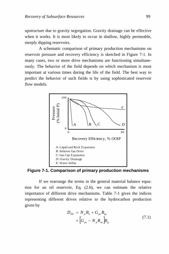
Recovery of Subsurface Resources 99
upstructure due to gravity segregation. Gravity drainage can be effective when it works. It is most likely to occur in shallow, highly permeable, steeply dipping reservoirs. A schematic comparison of primary production mechanisms on reservoir pressure and recovery efficiency is sketched in Figure 7-1. In many cases, two or more drive mechanisms are functioning simultane-ously. The behavior of the field depends on which mechanism is most important at various times during the life of the field. The best way to predict the behavior of such fields is by using sophisticated reservoir flow models.
Pre
ssu
re(%
Initi
alP
)
100
00 60
A B C D
E
Recovery Efficiency, % OOIP
A: Liquid and Rock ExpansionB: Solut ion Gas DriveC: Gas Cap ExpansionD: Gravity DrainageE: Water Influx
Figure 7-1. Comparison of primary production mechanisms
If we rearrange the terms in the general material balance equa-tion for an oil reservoir, Eq. (2.6), we can estimate the relative importance of different drive mechanisms. Table 7-1 gives the indices representing different drives relative to the hydrocarbon production given by
[ ] gsopps
gcpcopHC
BRNG
BGBND
−+
+= (7.1)

100 Principles of Applied Reservoir Simulation
Table 7-1 Drive Indices from the Schilthuis Material Balance Equation
Drive Index
Solution Gas Isg = NDo / DHC
Gas Cap Igc = NDgo / DHC
Water Iw = [(We - Wp)Bw] / DHC
Injected Fluids I i = [WiBw + GiB′g] / DHC
Connate Water and Rock Expansion Ie = [N(Dw + Dgw) + NDr] / DHC
The sum of the drive indices equals one, thus
1=++++ eiwgcsg IIIII (7.2)
Equation (7.2) can be derived by rearranging Eq. (2.6). A comparison of the magnitudes of the drive indices indicates which drive is dominating the performance of the reservoir. If the sum of the drive indices in Eq. (7.2) does not equal one based on available data, Pletcher [2002, page 49] has cautioned that the drive indices should not be normalized to one because this may obscure the usefulness of the drive indices and “lead to a false sense of security.” Although the above discussion refers to oil reservoirs, similar comments apply to gas reservoirs. Water drive and gas expansion with reservoir pressure depletion are the most common drives for gas reser-voirs. Gas reservoir recovery can be as high as 70% to 90% of original gas in place (OGIP) because of the high mobility of gas relative to oil mobility. Gas storage reservoirs have a different life cycle than gas reser-voirs that are being depleted. Gas storage reservoirs are used as a warehouse for gas. If the gas is used as a fuel for power plants, it will also need to be periodically produced and replenished. The performance attributes of a gas storage reservoir are [Tek, 1996, pg. 4]:

Recovery of Subsurface Resources 101
Ü Verification of inventory Ü Assurance of deliverability Ü Containment against migration
The gas inventory consists of working gas and cushion gas. Gas deliver-ability must be sufficient to account for swings in demand. Demand can vary daily and seasonally. Gas containment is needed to conserve the amount of stored gas. For more discussion of natural gas storage in res-ervoirs, see references such as Tek [1996], Smith [1990], and Katz and Lee [1990].
7.1.2 Secondary Production Primary depletion is usually not sufficient to optimize recovery from an oil reservoir. Oil recovery can be both accelerated and increased by supplemental natural reservoir energy. The supplemental energy is provided using an external energy source, such as water injection or gas injection. The injection of water or natural gas may be referred to as pressure maintenance or secondary production. The latter term arose be-cause injection usually follows a period of primary pressure depletion, and is therefore the second production method used in a field. Many modern reservoirs incorporate pressure maintenance early in the produc-tion life of the field, sometimes from the beginning of production. In this case the reservoir is not subjected to a conventional primary production phase. The term pressure maintenance more accurately describes the reservoir management strategy for these fields than the term secondary
production.
7.1.3 Alternative Classifications Both primary and secondary recovery processes are designed to produce oil using immiscible methods. Additional methods may be used to improve oil recovery efficiency by reducing residual oil saturation. The reduction of residual oil saturation requires a change in such factors

102 Principles of Applied Reservoir Simulation
as interfacial tension (IFT) or wettability. Methods designed to reduce residual oil saturation have been referred to in the literature as:
Ü Tertiary Production Ü Enhanced Oil Recovery Ü Improved Oil Recovery
The term tertiary production was originally used to identify the third stage of the production life of the field. Typically the third stage oc-curred after waterflooding. The third stage of oil production would involve a process that was designed to mobilize waterflood residual oil. An example of a tertiary production process is a chemical flood process such as surfactant flooding.
Tertiary production processes were designed to improve dis-placement efficiency by injecting fluids or heat. They were referred to as enhanced recovery processes. It was soon learned, however, that some fields would perform better if the enhanced recovery process was im-plemented before the third stage in the life of the field. In addition, it was found that enhanced recovery processes were often more expensive than just drilling more wells in a denser pattern. The drilling of wells to reduce well spacing and increase well density is called infill drilling. The birth of the term infill drilling was coincident with the birth of another term, improved recovery, which in-cludes enhanced oil recovery and infill drilling. Some major improved recovery processes are waterflooding, gasflooding, chemical flooding, and thermal recovery [Dyke, 1997]. They are discussed in more detail below.
7.2 Enhanced Oil Recovery Improved recovery technology includes traditional secondary recovery processes such as waterflooding and immiscible gas injection, as well as enhanced oil recovery (EOR) processes. EOR processes are usually classified as follows: chemical, miscible, thermal, and microbial.

Recovery of Subsurface Resources 103
A brief description of each of these processes is presented below. The success of an EOR project depends on good planning. Hite, et al. [2005] recommend the following steps for planning an EOR project [para-phrased from Hite, et al., 2005, page 28]: 1. Identify the appropriate EOR process 2. Characterize the reservoir 3. Determine engineering design parameters 4. Conduct pilot or field tests as needed 5. Finish with a plan to manage the project Reservoir flow models are an important tool in the EOR project planning process.
The literature on EOR is extensive. For more detailed discus-sions of EOR, including screening criteria and analyses of displacement mechanisms, see such references as Taber and Martin [1983], Lake [1989], Martin [1992], Taber, et al. [1997a,b], and Green and Willhite [1998].
7.2.1 Chemical
Chemical flooding methods include polymer flooding, micellar-polymer flooding or surfactant-polymer flooding, and alkaline or caustic flooding. Polymer flooding is designed to improve the mobility ratio and fluid flow patterns of a displacement process by increasing the viscosity of the injected aqueous phase. In this case, high molecular weight poly-mer is added to injected water. Micellar-polymer flooding uses a detergent-like solution to lower residual oil saturation to waterflooding. The polymer slug injected after the micellar slug is designed to improve displacement efficiency. Alkaline flooding uses alkaline chemicals that can react with certain types of in situ crude. The resulting chemical product is miscible with the oil and can reduce residual oil saturation to waterflooding.
104 Principles of Applied Reservoir Simulation
7.2.2 Miscible Miscible flooding methods include carbon dioxide injection, natural gas injection, and nitrogen injection. Miscible gas injection must be performed at a high enough pressure to ensure miscibility between the injected gas and in situ oil. Miscibility is achieved when interfacial ten-sion (IFT) between the aqueous and oleic phases is significantly reduced. The desired IFT reduction is typically from around 1 dyne/cm to 0.001 dyne/cm or less. Any reduction in IFT can improve displacement effi-ciency, and a near miscible process can yield much of the incremental oil that might be obtained from a miscible process. If reservoir pressure is not maintained above the minimum miscibility pressure (MMP) of the system, the gasflood will be an immiscible gas injection process. Immiscible gas can be used as the principal injection fluid in a secondary displacement process, or it can be used as the injection fluid for a tertiary process. Two improved recovery processes based on im-miscible gas injection are the double displacement process (DDP) and the second contact water displacement (SCWD) process [Novakovic, 1999]. Both processes require the injection of immiscible gas into reser-voirs that have been previously waterflooded. The processes require favorable gas-oil and oil-water interfacial tensions. Oil remaining after waterflood can coalesce into a film when exposed to an immiscible gas. The oil film can be mobilized and produced by downdip gravity drainage (the DDP process) or by water influx from either an aquifer or water in-jection (SCWD) following the immiscible gas injection period.
7.2.3 Thermal Thermal flooding methods include hot water injection, steam drive, steam soak, and in situ combustion. The injection or generation of heat in a reservoir is designed to reduce the viscosity of in situ oil and improve the mobility ratio of the displacement process. Electrical meth-ods can also be used to heat fluids in relatively shallow reservoirs containing high viscosity oil, but electrical methods are not as common
Recovery of Subsurface Resources 105
as hot fluid injection methods. The in situ combustion method requires compressed air injection after in situ oil has been ignited. Steam injection methods require the injection of steam into a reservoir. Steam and hot water injection processes are the most common thermal methods because of the relative ease of generating hot water and steam. The in situ com-bustion process is more difficult to control than steam injection processes and it requires in situ oil that can be set on fire. Hot gases and heat ad-vance through the formation and displace the heated oil to production wells.
7.2.4 Microbial Microbial EOR uses the injection of microorganisms and nutri-ents in a carrier medium to increase oil recovery, reduce water production in petroleum reservoirs, or both. Dietrich, et al. [1996] sum-marized the results of five successful commercial microbial EOR projects. The projects reflected a diversity of locations, lithologies, depths, porosities, permeabilities, and temperatures. Two of the projects were in the United States, two were in China, and one was in Argentina. The projects included sandstone, fractured dolomite, siltstone-sandstone, and fractured sandstone reservoirs. Reservoir depths ranged from 4450 ft. to 6900 ft., temperatures from 110° F to 180° F, porosity from 0.079 to 0.232, and effective permeability from 1.7 md to 300 md. Evidence from laboratory research and field case studies shows that microbial EOR processes can result in the incremental recovery of oil and also re-duce water production from high permeability zones. However, research is continuing to maximize the technical and economic potential for mi-crobial EOR. For example, the U.S. Department of Energy has underwritten the development of microbial transport simulators.
7.3 Unconventional Fossil Fuels Oil and gas fields are considered conventional sources of fossil fuels. In the following, we discuss several unconventional sources of
106 Principles of Applied Reservoir Simulation
fossil fuels. The unconventional sources are becoming a more important part of the global energy mix as the price of oil increases.
7.3.1 Coalbed Methane
Coalbeds are an abundant source of methane [Selley, 1998; Rogers, 1994]. The presence of methane gas in coal has been well known to coal miners as a safety hazard, but is now being viewed as a source of natural gas. The gas is bound in the micropore structure of the coalbed. It is able to diffuse into the natural fracture network when a pressure gradi-ent exists between the matrix and the fracture network. The fracture network in coalbeds consists of microfractures. Coalbed microfractures allow Darcy flow and are called “cleats.” Gas recovery from coalbeds depends on three processes [Kuusk-raa and Brandenburg, 1989]. Coalbed methane exists as a monomolecul-ar layer on the internal surface of the coal matrix. Its composition is predominately methane, but can also include other constituents, such as ethane, carbon dioxide, nitrogen and hydrogen [Mavor, et al., 1999]. For this reason, coalbed methane is also known as coal gas to highlight the observation that gas from coalbeds is usually a mixture. Gas content can range from approximately 20 standard cubic feet (SCF) gas per ton of coal in the Powder River Basin of Wyoming [Mavor, et al., 1999] to 600 SCF per ton in the Appalachian Basin [Gaddy, 1999].
Gas recovery begins with desorption of gas from the internal sur-face to the coal matrix and micropores. The gas then diffuses through the coal matrix and micropores into the cleats. Finally, gas flows through the cleats to the production well. The flow rate depends, in part, on the pres-sure gradient in the cleats and the density and distribution of cleats. The controlling mechanisms for gas production from coalbeds are the rate of desorption from the coal surface to the coal matrix, the rate of diffusion from the coal matrix to the cleats, and the rate of flow of gas through the cleats. The flow rate in the cleats obeys Darcy’s Law in many systems, but may also depend on stress-dependent permeability or gas slippage (the Klinkenberg effect). Shi and Durucan [2005] discuss the dependence
Recovery of Subsurface Resources 107
of coalbed permeability on stress. Stress-dependent permeability in oil and gas fields is discussed in more detail in Chapter 14. The production performance of a well producing gas from a coalbed will typically exhibit three stages. The reservoir dewaters and methane production increases during the first stage of pressure depletion. Methane production peaks during the second stage. The amount of water produced is relatively small compared to gas production during the sec-ond stage because of gas-water relative permeability effects, and desorption of natural gas provides a counterbalance to permeability loss as a result of formation compaction. The third stage of production is similar to conventional gas field production in which gas rate declines as reservoir pressure declines.
Coalbed methane recovery can be enhanced by injecting carbon dioxide into the coal seam. Carbon dioxide preferentially displaces meth-ane in the coal matrix. The displaced methane can then be produced through the cleat system. The resulting adsorption of carbon dioxide by coal can be used to sequester, or store, carbon dioxide in the coal seam. Carbon dioxide sequestration has an environmental benefit that is dis-cussed in more detail in Chapter 8.
7.3.2 Gas Hydrates
The entrapment of natural gas molecules in ice at very low tem-peratures forms an ice-like solid which is a metastable complex called a gas hydrate. Gas hydrates are clathrates. A clathrate is a chemical com-plex that is formed when one type of molecule completely encloses another type of molecule in a lattice. In the case of gas hydrates, hydro-gen-bonded water molecules form a cage-like structure in which mobile molecules of gas are absorbed or bound. The presence of gas hydrates can complicate field operations. For example, the existence of hydrates on the ocean floor can affect drill-ing operations in deep water. The simultaneous flow of natural gas and water in tubing and pipelines can result in the formation of gas hydrates that can impede or completely block the flow of fluids through pipeline

108 Principles of Applied Reservoir Simulation
networks. Heating the gas or treating the gas-water system with chemical inhibitors can prevent the formation of hydrates, but increases operating costs. Gas hydrates are generally considered a problem for oil and gas field operations, but their potential commercial value as a clean energy resource is changing industry perception. The potential as a gas resource is due to the relatively large volume of gas contained in the gas hydrate complex. In particular, Makogon, et al. [1997] have reported that one cubic meter of gas hydrate contains 164.6 m3 of methane. This is equiva-lent to one barrel of gas hydrate containing 924 ft3 of methane, and is approximately six times as much gas as the gas contained in an unim-peded gas-filled pore system [Selley, 1998, pg. 25]. The gas in gas hydrates occupies approximately 20% of the volume of the gas hydrate complex. Water occupies the remaining 80% of the gas hydrate complex volume. Gas hydrates can be found throughout the world [Selley, 1998; Makogon, et al., 1997]. They exist on land in sub-Arctic sediments and on seabeds where the water is near freezing at depths of at least 600 to 1500 feet. For instance, favorable conditions for gas hydrate formation
exist at sea floor temperatures as low as 39°F in the Gulf of Mexico and
as low as 30°F in some sections of the North Sea. According to Ma-
kogon, et al. [1997], over 700 trillion m3 in explored reserves of methane in the hydrate state exist. Difficulties in cost effective production have hampered development of the resource.
7.3.3 Tight Gas Sands and Shale Gas
Unconventional gas resources include coalbed methane, tight gas sands and fractured gas shales. Coalbed methane was discussed above. Both tight gas sands and gas shales are characterized by low permeabili-ties, that is, permeabilities that are a fraction of a millidarcy. The low permeability associated with unconventional gas resources makes it more difficult to produce the gas at economical rates.

Recovery of Subsurface Resources 109
Economic production of gas from a gas shale or tight gas sand often requires the creation of fractures by a process known as hydraulic fracturing [Wattenbarger, 2002; Kuuskraa and Bank, 2003]. In this proc-ess, a fluid is injected into the formation at a pressure that exceeds the fracture pressure of the formation. Once fractures have been created in the formation, a proppant such as manmade pellets or coarse grain sand is injected into the fracture to prevent it from closing, or healing, when the injection pressure is removed. The proppant provides a higher per-meability flow path for gas to flow to the production well. Unconventional low permeability gas sands and shales often require more wells per unit area than conventional higher permeability gas res-ervoirs. The key to managing an unconventional gas resource is to develop the resource with enough wells to maximize gas recovery with-out drilling unnecessary wells.
7.3.4 Shale Oil and Tar Sands
Shale oil is high API gravity oil contained in porous, low perme-ability shale. Sand grains that are cemented together by tar or asphalt are called tar sands. Tar and asphalt are highly viscous, plastic or solid hy-drocarbons. Extensive shale oil and tar sand deposits are found throughout the Rocky Mountain region of North America, as well as in other parts of the world. Although difficult to produce, the volume of hydrocarbon in tar sands has stimulated efforts to develop production techniques.
The hydrocarbon in shale oil and tar sands can be extracted by mining when they are close enough to the surface. Tar pits have been found around the world and have been the source of many fossilized di-nosaur bones. In locations where oil shale and tar sands are too deep to mine, it is necessary to increase the mobility of the hydrocarbon.
An increase in permeability or a decrease in viscosity can in-crease mobility. Increasing the temperature of high API gravity oil, tar or asphalt can significantly reduce viscosity. If there is enough permeability to allow injection, steam or hot water can be used to increase formation

110 Principles of Applied Reservoir Simulation
temperature and reduce hydrocarbon viscosity. In many cases, however, permeability is too low to allow significant injection of a heated fluid. An alternative to fluid injection is electromagnetic heating. Radio fre-quency heating has been used in Canada, and electromagnetic heating techniques are being developed for other parts of the world.
7.4 IFLO Coal Gas Model
The coal gas model in IFLO is designed to model production of gas from coalbeds. Gas desorption from the coal matrix into the cleat system during depletion of a coal seam is included in the reservoir simu-lator flow equations as a gas desorption rate qcg. Coal gas desorption is modeled as a process that obeys Fick’s law of diffusion, namely
cc rrt
C
r
Cr
rrD ≤<
∂∂
=⎥⎦
⎤⎢⎣
⎡∂∂
∂∂
0,1 22
(7.3)
where Dc is the diffusion coefficient, r is radius in spherical coordinates, rc is the radius of a spherical coal particle, and C is the gas content of coal in SCF of gas per ton of coal. The diffusion process obeys the initial and boundary conditions
( ) ( )PGtrCr
Ccc
r
==∂∂
=
,;00
(7.4)
where the coal gas content Gc(P) is a function of pressure given by the Langmuir isotherm
PP
PVG
LLc +
= (7.5)
The parameters VL and PL are the Langmuir volume and Langmuir pres-sure respectively.
The diffusion equation, Eq. (7.3), is first solved for the gas con-tent C(r,t). The rate of gas desorption qcg is calculated from C(r,t) as
crc
ccccg r
C
r
DVq
∂∂
ρ=3
(7.6)

Recovery of Subsurface Resources 111
where Vc is the volume of coal and ρc is coal density [Ancell, et al.,
1980; King and Ertekin, 1995]. The ratio Dc/rc in Eq. (7.6) is called the diffusivity of the coal seam. A finite difference representation of the de-
rivative ∂C(r,t)/∂r is then used to calculate qcg. The user directly enters
the parameters Dc, rc, ρc, VL and PL. The coal volume Vc is calculated
from the reservoir description provided by the user.
7.4.1 Critical Desorption Pressure
Gas content Gc in saturated coal seams is given by the Langmuir isotherm, Eq. (7.5). A coal seam is undersaturated if the laboratory measured gas content corresponds to a pressure on the Langmuir iso-therm that is less than the initial reservoir pressure measured by a well test. To handle this case, the user may enter a critical desorption pressure PCD. If the undersaturated coal gas model is selected, the gas content will depend on PCD. In particular, gas content Gc at PCD will be used when coal seam pressure P > PCD, otherwise gas content Gc will be calculated at P.
7.5 IFLO Application: Coal Gas Production from a Fruitland Coal
We illustrate the application of the coal gas model to a scenario
published by Paul, et al. [1990]. They presented a model of two coal lay-ers with Fruitland coal formation properties separated by a sandstone layer. Properties for each layer in the Fruitland coal model are presented in Table 7-2. The Fruitland coal is in the San Juan Basin in the Four Cor-ners region of the United States. The Four Corners region is located where the states of Utah, Colorado, New Mexico, and Arizona have a common border. Both coal layers are water saturated while the sandstone layer has a free gas saturation of 15%. An impermeable layer separates
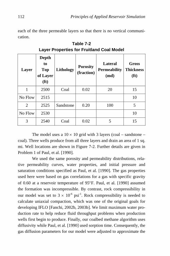
112 Principles of Applied Reservoir Simulation
each of the three permeable layers so that there is no vertical communi-cation.
Table 7-2 Layer Properties for Fruitland Coal Model
Layer
Depth to
Top of Layer
(ft)
LithologyPorosity (fraction)
Lateral Permeability
(md)
Gross Thickness
(ft)
1 2500 Coal 0.02 20 15
No Flow 2515 10
2 2525 Sandstone 0.20 100 5
No Flow 2530 10
3 2540 Coal 0.02 5 15
The model uses a 10 × 10 grid with 3 layers (coal – sandstone – coal). Three wells produce from all three layers and drain an area of 1 sq. mi. Well locations are shown in Figure 7-2. Further details are given in Problem 1 of Paul, et al. [1990].
We used the same porosity and permeability distributions, rela-tive permeability curves, water properties, and initial pressure and saturation conditions specified as Paul, et al. [1990]. The gas properties used here were based on gas correlations for a gas with specific gravity
of 0.60 at a reservoir temperature of 95°F. Paul, et al. [1990] assumed
the formation was incompressible. By contrast, rock compressibility in
our model was set to 3 × 10⁻⁶ psi-1. Rock compressibility is needed to calculate uniaxial compaction, which was one of the original goals for developing IFLO [Fanchi, 2002b, 2003b]. We limit maximum water pro-duction rate to help reduce fluid throughput problems when production wells first begin to produce. Finally, our coalbed methane algorithm uses diffusivity while Paul, et al. [1990] used sorption time. Consequently, the gas diffusion parameters for our model were adjusted to approximate the
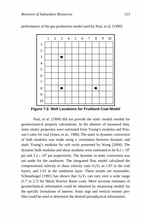
Recovery of Subsurface Resources 113
performance of the gas production model used by Paul, et al. [1990].
1 2 3 4 5 6 7 8 9 10
1
2
3
4
5
6
7
8
9
10
Figure 7-2. Well Locations for Fruitland Coal Model
Paul, et al. [1990] did not provide the static moduli needed for geomechanical property calculations. In the absence of measured data, static elastic properties were estimated from Young’s modulus and Pois-son’s ratio for coal [Jones, et al., 1988]. The static to dynamic conversion of bulk modulus was made using a correlation between dynamic and static Young’s modulus for soft rocks presented by Wang [2000]. The
dynamic bulk modulus and shear modulus were estimated to be 8.2 × 10⁵
psi and 3.2 × 10⁵ psi respectively. The dynamic to static conversion was
not made for the sandstone. The integrated flow model calculated the compressional velocity to shear velocity ratio VP/VS as 1.97 in the coal layers, and 1.61 in the sandstone layer. These results are reasonable. Schraufnagel [1991] has shown that VP/VS can vary over a wide range (1.7 to 2.7) for Black Warrior Basin coals. More accurate estimates of geomechanical information could be obtained by measuring moduli for the specific formations of interest. Sonic logs and vertical seismic pro-files could be used to determine the desired petrophysical information.

114 Principles of Applied Reservoir Simulation
Figure 7-3 shows gas and water production rates for this sce-nario. The sharp increases in water rate show when each water production well begins to produce. The water rate declines sharply as gas desorbs from the coal and flows through the cleat system to the wells.
0
200
400
600
800
1000
1200
1400
1600
1800
2000
0 500 1000 1500 2000 2500 3000 3500 4000
Days
Ga
s R
ate
(M
SC
F/D
)
0
200
400
600
800
1000
1200
Wat
er R
ate
(ST
B/D
)
Gas Water
Figure 7-3. Gas and Water Rates for Production from Fruitland Coal
Exercises
Exercise 7.1 Use the definitions in Table 7-1 and Eq. (7-1) to derive Eq. (7-2) from Eq. (2.6). Exercise 7.2A Which drive index in Table 7-1 will be largest in a field containing dead oil that is subjected to pressure depletion? Exercise 7.2B Suppose a dead oil reservoir is subjected to a peripheral waterflood. Identify the two drive indices in Table 7-1 that will have the greatest influence on oil recovery. Exercise 7.3A List the letters of the following recovery processes that are considered improved oil recovery methods.

Recovery of Subsurface Resources 115
a. steamflood e. in situ combustion
b. solution gas drive f. microbial EOR
c. waterflood g. water drive by aquifer influx
d. miscible gas injection h. polymer flooding
Exercise 7.3B List the letters of the recovery processes in Problem #3 that are considered enhanced oil recovery processes. Exercise 7.4 What are the three stages of production performance for a coalbed methane well? Exercise 7.5A A coal seam is 800 feet wide, 1 mile long, and 10 feet thick. The volume occupied by the fracture network is 1%. What is the volume of coal in the coal seam? Express your answer in ft3 and m3. Exercise 7.5B If the density of coal is 1.7 lbm/ft3, how many tonnes of coal are in the coal seam? Note that 1 ton = 2000 lbm = 907 kg = 0.907 tonne.
Exercise 7.6A Assume the Langmuir isotherm G VP
P Pc LL
=+
for a
coal seam has a Langmuir volume of 600 standard cubic feet per ton of coal (SCF/ton) and a Langmuir pressure of 450 psia. Calculate the vol-ume of gas per ton of coal at a pressure of 1000 psia. Express your answer in SCF/ton where 1 ton = 2000 lbm. Exercise 7.6B How much gas is contained in the coal? Assume the mass
of coal is mass tonnecoal = ×322 104. . Express your answer in SCF
and cubic meters. Note that 1 ton = 2000 lbm = 907 kg = 0.907 tonne. Exercise 7.7 Some EOR simulators can be found on the internet. Access the internet and search for a website containing public domain EOR simulators. Hint: The United States Department of Energy is one gov-ernmental agency that has distributed EOR software using a website.

116 Principles of Applied Reservoir Simulation
Exercise 7.8 Run file CBM_SPE20733-1_PVTG.dat and plot gas pro-duction rate and water production rate as functions of time.

117
Chapter 8
Economics and the Environment Economic analyses are an essential aspect of a reservoir man-agement study. The economic performance of a prospective project is often the deciding factor in determining whether to undertake a project. Consequently, it is important to be aware of basic economic concepts and factors that may affect the economic performance of a project. These topics are introduced here. Further details can be found in references such as Thompson and Wright [1985], Satter and Thakur [1994], Seba [1998], and Newendorp and Schuyler [2000].
8.1 Society of Petroleum Engineers and World Petroleum Congress Reserves
The analysis of a petroleum project depends on the amount of commercially valuable resource that is available. According to the Soci-ety of Petroleum Engineers (SPE) and the World Petroleum Congress (WPC) [Staff-JPT, 1997], reserves are those quantities of petroleum that are anticipated to be commercially recoverable from known accumula-tions from a given date forward. Table 8-1 summarizes the SPE/WPC definitions of reserves which include both qualitative and quantitative criteria. Although the SPE/WPC definitions have been adopted in many parts of the world, they are not universal. For example, a different, yet
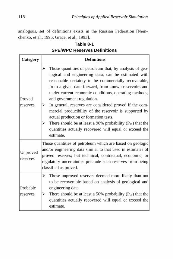
118 Principles of Applied Reservoir Simulation
analogous, set of definitions exists in the Russian Federation [Nem-chenko, et al., 1995; Grace, et al., 1993].
Table 8-1 SPE/WPC Reserves Definitions
Category Definitions
Proved reserves
Ü Those quantities of petroleum that, by analysis of geo-logical and engineering data, can be estimated with reasonable certainty to be commercially recoverable, from a given date forward, from known reservoirs and under current economic conditions, operating methods, and government regulation.
Ü In general, reserves are considered proved if the com-mercial producibility of the reservoir is supported by actual production or formation tests.
Ü There should be at least a 90% probability (P90) that the quantities actually recovered will equal or exceed the estimate.
Unproved reserves
Those quantities of petroleum which are based on geologic and/or engineering data similar to that used in estimates of proved reserves; but technical, contractual, economic, or regulatory uncertainties preclude such reserves from being classified as proved.
Probable reserves
Ü Those unproved reserves deemed more likely than not to be recoverable based on analysis of geological and engineering data.
Ü There should be at least a 50% probability (P50) that the quantities actually recovered will equal or exceed the estimate.

Economics and the Environment 119
Possible reserves
Ü Those unproved reserves deemed less likely to be re-coverable than probable reserves based on analysis of geological and engineering data.
Ü There should be at least a 10% probability (P10) that the quantities actually recovered will equal or exceed the estimate.
The probability distribution associated with the SPE/WPC re-serves definitions can be estimated with relative ease if the modeling team has performed a sensitivity analysis that generates a set of cases that yield low, medium, and high reserve estimates. In the absence of data to the contrary, a reasonable first approximation is that each case is equally likely to occur. Given this assumption, an average µ and standard
derivation σ may be calculated from the sensitivity analysis results to
prepare a normal distribution of reserves. For a normal distribution with
mean µ and standard deviation σ, the SPE/WPC reserves definitions are quantified as follows:
Proved reserves =P90 = µ - 1.28 σ
Probable reserves =P50 = µ
Possible reserves =P10 = µ + 1.28 σ
The normal distribution can be used to associate an estimate of the like-lihood of occurrence of any particular prediction case with its corresponding economic forecast. Keep in mind, however, that the actual distribution of reserves may not be normal, and that a detailed analysis of the distribution may be needed in many cases.
8.2 Basic Economic Concepts The cash flow of a project is the net cash generated or expended on the project as a function of time. The time value of money is included in economic analyses by applying a discount rate to adjust the value of money to the value during a base year. Discount rate is the adjustment
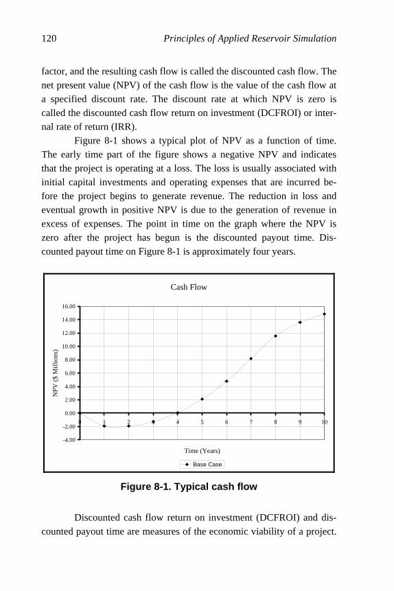
120 Principles of Applied Reservoir Simulation
factor, and the resulting cash flow is called the discounted cash flow. The net present value (NPV) of the cash flow is the value of the cash flow at a specified discount rate. The discount rate at which NPV is zero is called the discounted cash flow return on investment (DCFROI) or inter-nal rate of return (IRR). Figure 8-1 shows a typical plot of NPV as a function of time. The early time part of the figure shows a negative NPV and indicates that the project is operating at a loss. The loss is usually associated with initial capital investments and operating expenses that are incurred be-fore the project begins to generate revenue. The reduction in loss and eventual growth in positive NPV is due to the generation of revenue in excess of expenses. The point in time on the graph where the NPV is zero after the project has begun is the discounted payout time. Dis-counted payout time on Figure 8-1 is approximately four years.
Cash Flow
-4.00
-2.00
0.00
2.00
4.00
6.00
8.00
10.00
12.00
14.00
16.00
0 1 2 3 4 5 6 7 8 9 10
Time (Years)
NP
V (
$ M
illio
ns)
Base Case
Figure 8-1. Typical cash flow
Discounted cash flow return on investment (DCFROI) and dis-counted payout time are measures of the economic viability of a project.
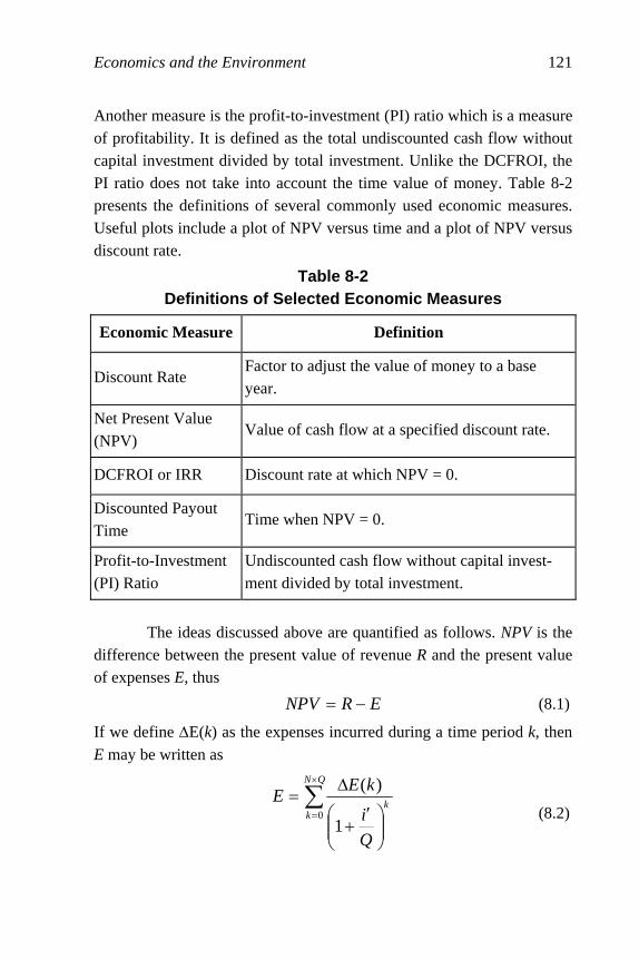
Economics and the Environment 121
Another measure is the profit-to-investment (PI) ratio which is a measure of profitability. It is defined as the total undiscounted cash flow without capital investment divided by total investment. Unlike the DCFROI, the PI ratio does not take into account the time value of money. Table 8-2 presents the definitions of several commonly used economic measures. Useful plots include a plot of NPV versus time and a plot of NPV versus discount rate.
Table 8-2 Definitions of Selected Economic Measures
Economic Measure Definition
Discount Rate Factor to adjust the value of money to a base year.
Net Present Value (NPV)
Value of cash flow at a specified discount rate.
DCFROI or IRR Discount rate at which NPV = 0.
Discounted Payout Time
Time when NPV = 0.
Profit-to-Investment (PI) Ratio
Undiscounted cash flow without capital invest-ment divided by total investment.
The ideas discussed above are quantified as follows. NPV is the difference between the present value of revenue R and the present value of expenses E, thus
ERNPV −= (8.1)
If we define ∆E(k) as the expenses incurred during a time period k, then E may be written as
∑×
=
⎟⎟⎠
⎞⎜⎜⎝
⎛ ′+
∆=
QN
kk
Q
i
kEE
01
)(
(8.2)
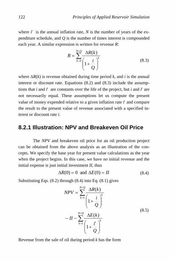
122 Principles of Applied Reservoir Simulation
where i′ is the annual inflation rate, N is the number of years of the ex-
penditure schedule, and Q is the number of times interest is compounded each year. A similar expression is written for revenue R:
∑×
=
⎟⎟⎠
⎞⎜⎜⎝
⎛+
∆=
QN
kk
Q
i
kRR
01
)(
(8.3)
where ∆R(k) is revenue obtained during time period k, and i is the annual
interest or discount rate. Equations (8.2) and (8.3) include the assump-
tions that i and i′ are constants over the life of the project, but i and i′ are
not necessarily equal. These assumptions let us compute the present
value of money expended relative to a given inflation rate i′ and compare the result to the present value of revenue associated with a specified in-terest or discount rate i.
8.2.1 Illustration: NPV and Breakeven Oil Price The NPV and breakeven oil price for an oil production project can be obtained from the above analysis as an illustration of the con-cepts. We specify the base year for present value calculations as the year when the project begins. In this case, we have no initial revenue and the initial expense is just initial investment II , thus
IIER =∆=∆ )0(nda0)0( (8.4)
Substituting Eqs. (8.2) through (8.4) into Eq. (8.1) gives
∑
∑
×
=
×
=
⎟⎟⎠
⎞⎜⎜⎝
⎛ ′+
∆−−
⎟⎟⎠
⎞⎜⎜⎝
⎛+
∆=
QN
kk
QN
kk
Q
i
kEII
Q
i
kRNPV
1
1
1
)(
1
)(
(8.5)
Revenue from the sale of oil during period k has the form
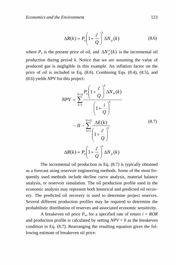
Economics and the Environment 123
)(1)( kNQ
iPkR p
k
o ∆⎟⎟⎠
⎞⎜⎜⎝
⎛ ′+=∆ (8.6)
where Po is the present price of oil, and )(kN op∆ is the incremental oil
production during period k. Notice that we are assuming the value of produced gas is negligible in this example. An inflation factor on the price of oil is included in Eq. (8.6). Combining Eqs. (8.4), (8.5), and (8.6) yields NPV for this project:
∑
∑
×
=
×
=
⎟⎟⎠
⎞⎜⎜⎝
⎛ ′+
∆−−
⎟⎟⎠
⎞⎜⎜⎝
⎛+
∆⎟⎟⎠
⎞⎜⎜⎝
⎛ ′+
=
QN
kk
QN
kk
P
k
o
Q
i
kEII
Q
i
kNQ
iP
NPV
1
1
1
)(
1
)(1
)(1)( kNQ
iPkR p
k
o ∆⎟⎟⎠
⎞⎜⎜⎝
⎛ ′+=∆
(8.7)
The incremental oil production in Eq. (8.7) is typically obtained as a forecast using reservoir engineering methods. Some of the most fre-quently used methods include decline curve analysis, material balance analysis, or reservoir simulation. The oil production profile used in the economic analysis may represent both historical and predicted oil recov-ery. The predicted oil recovery is used to determine project reserves. Several different production profiles may be required to determine the probabilistic distribution of reserves and associated economic sensitivity. A breakeven oil price Poe for a specified rate of return i = ROR and production profile is calculated by setting NPV = 0 as the breakeven condition in Eq. (8.7). Rearranging the resulting equation gives the fol-lowing estimate of breakeven oil price:
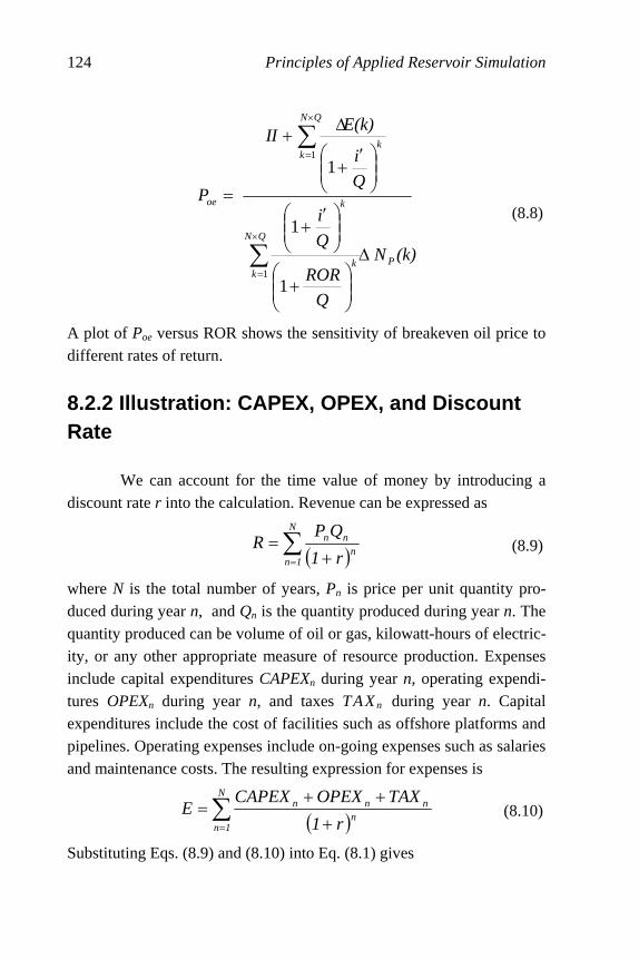
124 Principles of Applied Reservoir Simulation
∑
∑
×
=
×
=
∆
⎟⎟⎠
⎞⎜⎜⎝
⎛+
⎟⎟⎠
⎞⎜⎜⎝
⎛ ′+
⎟⎟⎠
⎞⎜⎜⎝
⎛ ′+
∆+
=
QN
kPk
k
QN
kk
oe
(k)N
Q
ROR
Q
i
Q
i
E(k)II
P
1
1
1
1
1
(8.8)
A plot of Poe versus ROR shows the sensitivity of breakeven oil price to different rates of return.
8.2.2 Illustration: CAPEX, OPEX, and Discount Rate
We can account for the time value of money by introducing a discount rate r into the calculation. Revenue can be expressed as
( )∑= +
=N
1nn
nn
r1
QPR (8.9)
where N is the total number of years, Pn is price per unit quantity pro-duced during year n, and Qn is the quantity produced during year n. The quantity produced can be volume of oil or gas, kilowatt-hours of electric-ity, or any other appropriate measure of resource production. Expenses include capital expenditures CAPEXn during year n, operating expendi-tures OPEXn during year n, and taxes TAXn during year n. Capital expenditures include the cost of facilities such as offshore platforms and pipelines. Operating expenses include on-going expenses such as salaries and maintenance costs. The resulting expression for expenses is
( )∑= +
++=
N
1nn
nnn
r1
TAXOPEXCAPEXE (8.10)
Substituting Eqs. (8.9) and (8.10) into Eq. (8.1) gives

Economics and the Environment 125
( )∑= +
−−−=
N
1nn
nnnnn
r1
TAXOPEXCAPEXQPNPV (8.11)
Equation (8.11) shows that NPV depends on the price of the resource, the quantity of the produced resource, discount rate, capital expenditures, operating expenditures, and taxes.
8.3 Investment Decision Analysis Economic analyses are performed to provide information about the economic performance we can expect from a project relative to alter-native investment options. The decision to invest in a project depends on many factors. Thompson and Wright [1985, pg. 3-2] list the following set of characteristics for measures of investment worth that can be used to compare and rank competing projects:
Ü Aligns with corporate goals. Ü Is easy to understand and apply. Ü Permits cost-effective decision making. Ü Provides a quantitative measure for acceptance or rejection. Ü Permits alternatives to be compared and ranked. Ü Incorporates the time value of money.
Economic analyses using indicators of economic performance provide information about the relative performance of different invest-ment options. Some commonly used economic measures are payout time, present worth, net present value, discount rate, profit-to-investment ratio, and internal rate of return. The economic measures that are used in investment decision analysis depend on the experience of the decision makers who will use them. The decision makers determine the relative importance of each economic measure.
Combinations of economic measures are often used as economic criteria for making decisions about projects. For example, a proposed project with an early payout but relatively low discount rate may be more

126 Principles of Applied Reservoir Simulation
attractive to a company that needs to maintain a positive cash flow than another project with a higher discount rate but that does not payout as soon. The criteria for acceptance or rejection of a project may change, even within a company, as the economic environment changes. It should be remembered, however, that quantitative indicators provide useful in-formation, but incomplete information. Economic viability is influenced by both tangible and intangible factors. Tangible factors such as drilling a well are relatively easy to quantify. Intangible factors such as environ-mental and socio-political concerns are relatively difficult to quantify, yet may be more important than tangible factors.
The future cost of some energy investment options may change significantly as a result of technological advances. The cost of a finite resource can be expected to increase as the availability of the resource declines, while the cost of an emerging technology will usually decline as the infrastructure for supporting the technology matures. Modern emerging technologies include advanced drilling techniques and time-lapse seismic analysis. Table 8-3 illustrates the sensitivity of oil produc-ing techniques to the price of oil. The table shows that more sophisticated technologies can be justified as the price of oil increases. It also includes a price estimate for alternative energy sources, such as wind and solar power. In some cases, technologies overlap. For example, steam flooding is an enhanced oil recovery (EOR) process that can com-pete with oil recovery techniques, while chemical flooding is an EOR process that can be as expensive as many alternative energy sources.
Table 8-3 Sensitivity of Oil Recovery Technology to Oil Price
Oil Recovery Technology Oil Price
(US$ per barrel in year 2000 US$)
Conventional 10 – 30
Enhanced Oil Recovery (EOR) 20 – 40
Extra Heavy Oil (e.g. tar sands) 25 – 45
Alternative Energy Sources 40 +

Economics and the Environment 127
Investment decision making depends on such factors as avail-ability, accessibility, environmental acceptability, capital cost, and ongoing operating expenses. The analysis of the costs associated with a project should take into account the initial capital expenditures and an-nual operating expenses for the life of the system. This analysis is called life cycle analysis. The initial costs of one proposed project may be rela-tively low compared to those of competing projects. If we only consider initial cost in our analysis, we may select a project that is not optimum. For example, the annual operating expenses for one project we might choose based on initial cost may be significantly larger than those for an alternative option. In addition, projections of future cost may be substan-tially in error if the cost of one or more of the components contributing to a project changes significantly in relation to our original estimate. To avoid making suboptimum decisions, we should consider all of the life cycle costs of each investment option, and evaluate the sensitivity of cash flow predictions to plausible changes in cost as a function of time.
8.3.1 Risk Analysis and Real Options Analysis
A characteristic of natural resource management is the need to understand the role of uncertainty in decision making. The information we have about a natural resource is usually incomplete. What informa-tion we do have may contain errors. Despite the limitations of our knowledge, we must often make important decisions to advance a pro-ject. These decisions should be made with the recognition that risk, or uncertainty, is present and can influence investment decisions. Here, risk refers to the possibility that an unexpected event can adversely affect the value of an asset. Uncertainty is not the same as risk. Uncertainty is the concept that our limited knowledge and understanding of the future does not allow us to predict the consequences of our decisions with 100% ac-curacy. Risk analysis is an attempt to quantify the risks associated with investing under uncertainty. One drawback of traditional risk analysis is the limited number of options that are considered. The focus of risk analysis is decision

128 Principles of Applied Reservoir Simulation
making based on current expectations about future events. For example, the net present value analysis discussed above requires forecasts of reve-nue and expenses based on today’s expectations. Technological advances or political instabilities are examples of events that may significantly alter our expectations. We might overlook or ignore options that would have benefited from the unforeseen events. An option in this context is a set of policies or strategies for making current and future decisions. Real Options Analysis attempts to incorporate some flexibility into the man-agement of investment options that are subject to considerable future uncertainty.
The best way to incorporate options into the decision making process is to identify them during the early stages of analysis. Once a set of options has been identified for a particular project, we can begin to describe the uncertainties and decisions associated with the project. By identifying and considering an array of options, we obtain a more com-plete picture of what may happen as a consequence of the decisions we make. Real Options Analysis helps us understand how important compo-nents of a project, particularly components with an element of uncertainty, influence the value of the project [Chorn and Croft, 2000].
8.4 Environmental Impact Environmental issues must always be considered in the devel-opment of a reservoir management strategy. For example, the Louisiana Offshore Oil Production (LOOP) facility is designed to keep the transfer of hydrocarbons between pipelines and tankers away from sensitive coastal areas. Periodic water sampling of surface and produced waters can assure that fresh water sources are not contaminated. In addition, periodic testing for the excavation or production of naturally occurring radioactive materials helps assure environmental compliance. A well managed field should be compatible with both the surface and subsurface environment. The advantages of operating a field with prudent consideration of environmental issues can pay economic divi-dends. In addition to improved public relations, sensitivity to

Economics and the Environment 129
environmental issues can minimize adverse environmental effects that may require costly remediation and financial penalties. Remediation of-ten takes the form of cleanup, such as the cleanup required after the oil spill from the Exxon-Valdez oil tanker in Alaska. Technologies are being developed to improve our ability to cleanup environmental pollutants. For example, bioremediation uses living microorganisms or their en-zymes to accelerate the rate of degradation of environmental pollutants [Westlake, 1999].
8.4.1 Sustainable Development
Failure to consider environmental issues adequately can lead to both tangible and intangible losses. Intangible losses are difficult to quantify, but can include loss of public support for an otherwise eco-nomically viable project. Tangible losses have more readily quantifiable economic consequences. For example, near- and long-term economic liabilities associated with potable water contamination can adversely af-fect project economics. It becomes a question of business ethics whether a practice that is legal but can lead to an adverse environmental conse-quence should nonetheless be pursued because a cost-benefit analysis showed that there were fewer economic liabilities than economic bene-fits. Typically, arguments to pursue an environmentally undesirable practice based on cost-benefit analyses do not adequately account for intangible costs. For example, the decision by Shell to dispose of the Brent Spar platform by sinking it in the Atlantic Ocean led to public out-rage in Europe in 1995. Reversing the decision and disassembling the platform for use as a quay in Norway resolved the resulting public rela-tions problem, but the damage had been done. The failure to anticipate the public reaction reinforced a lack of public confidence in the oil and gas industry, and helped motivate government action to regulate the de-commissioning of offshore platforms in northwestern Europe [Wilkinson, 1997; Offshore staff, 1998].

130 Principles of Applied Reservoir Simulation
The problem facing the industry is to learn how to achieve sus-tainable development. The concept of sustainable development was introduced in 1987 in a report prepared by the United Nations’ World Commission on Environment and Development [Brundtland, 1987]. The commission, known as the Brundtland Commission after chairwoman Gro Harlem Brundtland of Norway, said that societies should adopt a policy of sustainable development that allows them to meet their present needs while preserving the ability of future generations to meet their own needs.
Society desires, and industry is seeking to achieve, sustainable development. One industry response to environmental and social con-cerns in the context of sustainable development is the triple bottom line (TBL) [Whittaker, 1999]. According to this view, sustainable develop-ment must integrate social and environmental concerns into a develop-ment plan that optimizes economic profitability and value creation. The three components of sustainable development, and the three goals of the TBL, are economic prosperity, social equity, and environmental protec-tion. The focus of TBL is the creation of long-term shareholder value by recognizing that corporations are dependent on licenses provided by so-ciety to do business. Whittaker [1999, pg. 25] reports that “After a period of serious introspection following the Brent Spar debacle, Royal Dutch/Shell is perhaps the most enthusiastic supporter of TBL.” TBL policy includes the following key elements [Whittaker, 1999, pg. 25]:
Ü Performance measurements that include qualitative social indica-
tors and ecoefficiency measures (such as energy consumption and recycling) in addition to compliance and pollutant emis-sions.
Ü Development and implementation of strategies that will enable the industry to meet both future global energy needs and envi-ronmental objectives.
Ü Investment in natural gas, low or zero emissions fuels, and re-newable forms of energy.
Ü Improved communications with communities affected by opera-tions.

Economics and the Environment 131
Sustainable development takes into account the rights of future generations. It is possible to argue that future generations have no legal rights to current natural resources and are not entitled to any. From this perspective, each generation must do the best it can with available re-sources. On the other hand, many societies are choosing to adopt the value of preserving natural resources for future generations. National parks are examples of natural resources that are being preserved.
8.4.2 Global Climate Change
Measurements of ambient air temperature show a global warm-ing effect that corresponds to an increase in the average temperature of the Earth’s atmosphere. The increase in atmospheric temperature has been linked to the combustion of fossil fuels [Wigley, et al., 1996; Lide, 2002, page 14-32].
When a carbon-based fuel burns, carbon can react with oxygen and nitrogen in the atmosphere to produce carbon dioxide (CO2), carbon monoxide, and nitrogen oxides (often abbreviated as NOx). The combus-tion byproducts, including water vapor, are emitted into the atmosphere in gaseous form. Some of the gaseous byproducts are called greenhouse gases because they contribute to the greenhouse effect, illustrated in Fig-ure 8-2. Some of the incident solar radiation from the Sun is absorbed by the Earth, some is reflected into space, and some is captured by green-house gases in the atmosphere and reradiated as infrared radiation (heat). The reradiated energy would have escaped the Earth as reflected sunlight if greenhouse gases were not present in the atmosphere. Greenhouse gases include carbon dioxide, methane, and nitrous oxide, as well as other gases such as volatile organic compounds and hydrofluorocarbons.
Carbon dioxide (CO2) is approximately 83% of the greenhouse gases emitted by the United States as a percent of the mass of carbon or carbon equivalent. Wigley, et al. [1996] projected ambient CO2 concen-tration through the twenty-first century. Pre-industrial atmospheric CO2 concentration was approximately 288 parts per million. Atmospheric CO2 concentration is currently 340 parts per million. The concentration
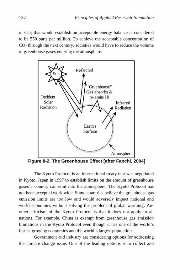
132 Principles of Applied Reservoir Simulation
of CO2 that would establish an acceptable energy balance is considered to be 550 parts per million. To achieve the acceptable concentration of CO2 through the next century, societies would have to reduce the volume of greenhouse gases entering the atmosphere.
Figure 8-2. The Greenhouse Effect [after Fanchi, 2004] The Kyoto Protocol is an international treaty that was negotiated
in Kyoto, Japan in 1997 to establish limits on the amount of greenhouse gases a country can emit into the atmosphere. The Kyoto Protocol has not been accepted worldwide. Some countries believe the greenhouse gas emission limits are too low and would adversely impact national and world economies without solving the problem of global warming. An-other criticism of the Kyoto Protocol is that it does not apply to all nations. For example, China is exempt from greenhouse gas emission limitations in the Kyoto Protocol even though it has one of the world’s fastest growing economies and the world’s largest population.
Government and industry are considering options for addressing the climate change issue. One of the leading options is to collect and
SunReflected
IncidentSolar
Radiation
Earth'sSurface
Atmosphere
InfraredRadiation
"Greenhouse"Gas absorbs &
re-emits IR

Economics and the Environment 133
store CO2 in reservoirs in a process known as geologic carbon sequestra-tion. The goal of geologic carbon sequestration and similar programs is to provide economically competitive and environmentally safe options to offset all projected growth in baseline emissions of greenhouse gases.
8.4.3 Subsidence
Subsidence is a compressibility effect that depends on the ge-omechanics of the produced interval and its overburden. Subsidence, or
the change in thickness ∆h of the reservoir, can be estimated from the compressibility and pressure depletion of the system using the equation
PhcPhch fB ∆φ=∆=∆
where
cB bulk compressibility (psia-1)
cf formation compressibility (psia-1)
h net thickness of reservoir (ft)
φ porosity (fraction)
∆P pressure depletion (psia)
If properties like compressibility are measured hydrostatically, they should be corrected to uniaxial compressibilities [Teeuw, 1971] so that the subsidence estimate becomes
Phch fu ∆φ⎟⎟⎠
⎞⎜⎜⎝
⎛ν−ν+
=∆1
1
3
1
where ν is Poisson’s ratio and the subscript u denotes uniaxial compac-
tion. The correction for uniaxial compaction recognizes that reservoirs with large lateral dimensions relative to their vertical thickness deform mainly in the vertical direction. In many cases, subsidence has little or no adverse environmental effects. In some cases, however, subsidence can be a significant concern. For example, a pressure maintenance program in a field where surface
134 Principles of Applied Reservoir Simulation
subsidence is a likely consequence of pressure depletion can improve resource recovery and help avoid economic liabilities resulting from damage caused by surface subsidence. Subsidence in the Long Beach, California, area due to production of the Wilmington field had to be mitigated with a pressure maintenance program. The pressure mainte-nance program can be as straightforward as water injection to replace the fluids that have been produced. Subsidence has been responsible for production induced seismic-ity in areas such as the Rocky Mountain Arsenal near Denver, Colorado, where production induced seismicity was identified as the cause of earthquakes. Earthquakes due to natural causes have led to fatalities in tectonically active areas like the Sea of Okhotsk, off Sakhalin Island, in Russia. Development activities in tectonically active areas, such as off-shore Sakhalin Island, need to anticipate the impact of subsidence and production induced seismicity as part of their reservoir management plans. Examples of compaction studies are presented by Teeuw [1971], Fredrich, et al. [1998], Settari and Walters [1999], Settari [2002], and Schutjens, et al. [2004].
8.5 IFLO Application: CO2 Sequestration in a Mature Oil Field
Reservoir flow modeling can be used to help manage geologic
carbon sequestration projects. Carbon dioxide may be sequestered in a variety of subsurface environments, such as CO2 injection into an oil field as part of an improved recovery process; CO2 injection into a ma-ture oil field as a storage process; CO2 injection into a coalbed to enhance coal gas recovery; and CO2 injection into an aquifer as a storage process. We demonstrate the application of reservoir flow modeling to the management of geologic carbon sequestration by modeling CO2 se-questration in a mature oil field [Fanchi, 2003b]. This application demonstrates enhanced oil recovery by miscible CO2 injection and CO2 sequestration.

Economics and the Environment 135
8.5.1 East Vacuum Grayburg/San Andres Unit
The Vacuum field was discovered in 1929. It is located about fif-teen miles west of Hobbs, New Mexico on the northwestern shelf of the Permian Basin and along the northern limit of the Delaware Basin [Brownlee and Sugg, 1987; Martin, et al., 1995]. Significant field devel-opment began in 1938 and was substantially completed in 1941. Waterflood development began in 1958. The East Vacuum Grayburg/San Andres Unit (EVGSAU) was formed in December 1978 and covers more than seven thousand acres on the eastern side of the Vacuum Field.
Oil with a gravity of 38°API has been produced from both the Grayburg and San Andres formations. The primary, productive interval at EVGSAU is the dolomitized carbonate sequence in the upper San Andres formation at a depth of approximately 4,400 ft. and a temperature of 101 °F. Infill drilling from forty-acre spacing to twenty-acre spacing in the EVGSAU began in 1979, and waterflooding began in 1980. The EVGSAU was converted to an eighty-acre inverted nine-spot pattern waterflood by 1982. A miscible CO2 injection project began in Septem-ber 1985, and a CO2-foam pilot test began in September 1991.
Grigg and Schechter [1998] prepared a history match of the CO2-foam pilot test area in the EVGSAU for the primary and waterflood periods (1959-1985). As part of their study, they published a model that included a characterization of the EVGSAU pilot area as well as satura-tion and pressure distributions at the end of waterflood. Their reservoir characterization was used to estimate the potential for sequestering CO2 in a mature oil field.
8.5.2 Sequestration Potential
The EVGSAU model uses a 3-D grid with 16×16×7 gridblocks. Figure 8-3 shows well placement in the model. The sides of each square gridblock are 240.5 feet long. The reservoir at the start of the run is in a pressure-depleted state: initial pore volume weighted average reservoir
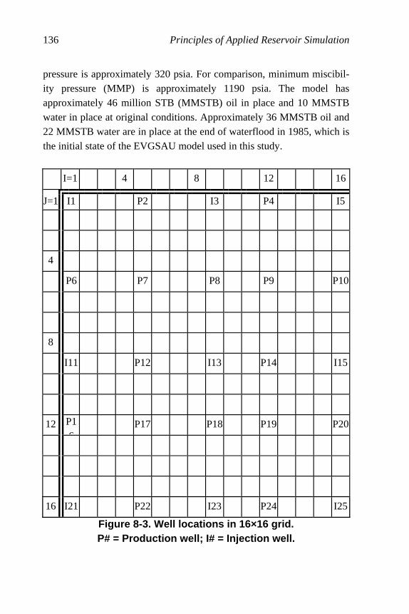
136 Principles of Applied Reservoir Simulation
pressure is approximately 320 psia. For comparison, minimum miscibil-ity pressure (MMP) is approximately 1190 psia. The model has approximately 46 million STB (MMSTB) oil in place and 10 MMSTB water in place at original conditions. Approximately 36 MMSTB oil and 22 MMSTB water are in place at the end of waterflood in 1985, which is the initial state of the EVGSAU model used in this study.
I=1 4 8 12 16
J=1 I1 P2 I3 P4 I5
4
P6 P7 P8 P9 P10
8
I11 P12 I13 P14 I15
12 P16
P17 P18 P19 P20
16 I21 P22 I23 P24 I25
Figure 8-3. Well locations in 16×16 grid. P# = Production well; I# = Injection well.

Economics and the Environment 137
We consider three sequestration cases. Case A evaluates the po-tential of injecting CO2 at immiscible conditions in the waterflooded zone. Immiscible CO2 injection begins at the start of the run and contin-ues for a period of ten years. In Case B, CO2 is used to raise reservoir pressure above minimum miscibility pressure and then conduct a misci-ble flood. In Case C, water injection is conducted for one year to raise reservoir pressure above MMP. The waterflood is then replaced by CO2 injection.
Table 8-4 shows the volume of CO2 sequestered after ten years of project life for both cases. Much more CO2 is sequestered if CO2 is injected into the reservoir at miscible pressure conditions than at immis-cible pressure conditions. More CO2 is sequestered in Case B than in Case C because Case C includes one year of water injection prior to nine years of CO2 injection. Although waterflooding delays CO2 sequestra-tion, waterflooding can improve time-lapse seismic monitoring. Time-lapse seismic monitoring is discussed in more detail in Part II.
Table 8-4 CO2 Sequestration at Ten Years
Case Injected Fluid CO2 In-jected
(BSCF)
CO2 Pro-duced
(BSCF)
CO2 Seques-tered
(BSCF)
A Immiscible Gas 65.1 51.9 13.2
B Miscible Gas 101.3 57.7 43.6
C Water then Miscible
Gas 92.1 51.4 40.7
Exercises
Exercise 8.1 Five independent studies determined the reserves for reser-voir A in the table below. Assuming a normal distribution of reserves, estimate proved, probable, and possible reserves. Hint: Calculate the av-erage and standard deviation for the oil recoveries reported above.

138 Principles of Applied Reservoir Simulation
Study 1 2 3 4 5
Oil Recovery (MSTBO) 320 150 480 260 370
Note: MSTBO denotes thousand stock tank barrels of oil. Exercise 8.2A What is life cycle analysis? Exercise 8.2B What is the purpose of Real Options Analysis? Exercise 8.3A Suppose the price of 1 liter of gasoline is US$1.10 in Europe. What is the price per gallon? Note: 1 L = 0.001 m3 and 1 gal =
3.785×10⁻³ m3.
Exercise 8.3B The price of gasoline is the sum of expenses plus taxes. If the expenses equal US$1.00 per gallon, what is the tax on a gallon of gasoline in Europe that has the price given in Part A? Exercise 8.4A If US$100 billion is spent on the military in a year to pro-tect the delivery of 20 million barrels of oil per day to the global market, how much does the military budget add to the cost of a barrel of oil? Exercise 8.4B How much is this cost per gallon? Exercise 8.5A What is geologic carbon sequestration? Exercise 8.5B What is the Kyoto Protocol? Exercise 8.6A How many barrels of oil would be needed to provide 100 quads of energy if the energy density of oil is 35,000 MJ/m3? Note: 1
quad = 1.055 × 10¹² MJ, 1 bbl = 0.1589 m3,
Exercise 8.6B If the volume of oil in Part A is consumed annually, what is the daily consumption of oil (in bbl)?
Economics and the Environment 139
Exercise 8.7A Suppose a reservoir has an average porosity of 20%, a formation compressibility of 20 x 10-6 psia-1, a net thickness of 500 feet, and the reservoir is subjected to a pressure depletion of 3000 psia. Plot subsidence as a function of Poisson’s ratio for a Poisson’s ratio ranging from 0.10 to 0.35. Exercise 8.7B If you are operating the field from a platform that is built with a deck that is 10 ft. above the maximum wave height, discuss the possible impact of subsidence on operations? Exercise 8.7C Discuss the possible impact of subsidence on wellbore stability for deviated wells drilled from the platform. Exercise 8.8A Typical reservoir values for formation, oil, water and gas compressibilities are
cf = 3 × 10⁶/psia
co = 10 × 106/psia
cw = 3 × 10⁶/psia
cg = 500 × 106/psia
Use the relationship P
V
Vc
∆∆
−=1
to estimate the fractional volume
change VV∆ of each substance for a pressure difference 〉P = Pfinal -
Pinitial = -100 psia. Exercise 8.8B Suppose oil saturation is 0.8 in an oil-water system. Cal-culate the bulk modulus of fluid assuming the compressibilities of oil and water are the values given above. Hint: first calculate water satura-tion and then calculate total fluid compressibility. Note that the bulk modulus of fluid is the inverse of fluid compressibility. Exercise 8.8C Suppose a formation has the following properties: Pois-son’s ratio is 0.2, porosity is 15%, and net thickness is 100 ft. Estimate

140 Principles of Applied Reservoir Simulation
subsidence for a pressure difference 〉P = Pfinal - Pinitial = -1000 psia and formation compressibility given in Part A. Exercise 8.9 File EVGSAU_MISC_WG.DAT is Case C of the IFLO sequestration study using the EVGSAU flow model. Run the file and determine the amount of CO2 sequestered at the end of the run. Hint: open the run output file ITEMP.ROF and find the cumulative injection and production of solvent 1. Solvent 1 is CO2 in this model. Exercise 8.10A File GOM_UNCONSOLIDATED.DAT is an example of production from unconsolidated sand in the Gulf of Mexico. Run the file and determine the maximum static uniaxial compaction at the end of the run. Hint: open the run output file ITEMP.ROF and find MAXIMUM STATIC UNIAXIAL COMPACTION at the end of the run. Exercise 8.10B Assume that the northern part of the reservoir is upstruc-ture and the southern part of the reservoir is downstructure. Is compaction greater on the west side of the reservoir or the east side of the reservoir at the end of the run?

141
Chapter 9
Multiphase Fluid Flow Equations The literature contains many derivations of the equations de-scribing fluid flow in porous media. Consequently, only a brief discussion will be presented here. We begin by introducing the continu-ity equation, and then present some important sets of fluid flow equations that are commonly used to model hydrocarbon reservoirs.
9.1 The Continuity Equation The continuity equation can be derived by considering the flow of fluid into and out of a single reservoir gridblock (Figure 9-1). Let the symbol J denote fluid flux. Flux is defined as the rate of flow of mass per unit cross-sectional area normal to the direction of flow, which is the x direction in the present case. Assume fluid flows into the gridblock at x
(Jx) and out of the gridblock at x + ∆x (Jx + ∆x). By conservation of mass,
we have the equality:
mass entering the gridblock − mass leaving the gridblock = accumulation of mass in the gridblock.
If the gridblock has length ∆x, width ∆y, and depth ∆z, we can write the
mass entering the gridblock in a time interval ∆t as
in Mass])()()[( =∆∆∆+∆∆+∆∆ tyxJzxJzyJ zzyyxx (9.1)

142 Principles of Applied Reservoir Simulation
where we have generalized the equation to allow flux in the y and z di-rections as well. The notation (Jx)x denotes the x direction flux at location x, with analogous meanings for the remaining terms.
Jx
∆ x
Jx+∆ x
y
x
z
Figure 9-1. Reservoir Gridblock: Coordinate Convention follows Sawyer and Mercer [1978]
Corresponding to mass entering is a term for mass exiting which has the form
out Mass
])()()[(
=∆∆∆∆+
∆∆∆+∆∆+∆∆ ∆+∆+∆+
tzyxq
tyxJzxJzyJ zzzyyyxxx(9.2)
We have added a source/sink term q which represents mass flow into (source) or out of (sink) a well. A producer is represented by q > 0, and an injector by q < 0. Accumulation of mass in the gridblock is the change in concen-
tration lC of phase l in the gridblock over the time interval ∆t. If the
concentration lC is defined as the total mass of phase l (oil, water, or
gas) in the entire reservoir gridblock divided by the gridblock volume, then the accumulation term becomes
( ) ( )[ ] onaccumulati Mass=∆∆∆−∆+ zyxCC ttt ll (9.3)
Using Eqs. (9.1) through (9.3) in the mass conservation equality
Mass in − Mass out = Mass accumulation

Multiphase Fluid Flow Equations 143
gives
( ) ( ) ( )[ ]( ) ( ) ( )[ ]
( ) ( )[ ] zyxCCtzyxq
tyxJzxJzyJ
tyxJzxJzyJ
ttt
zzzyyyxxx
zzyyxx
∆∆∆−=∆∆∆∆−
∆∆∆+∆∆+∆∆−
∆∆∆+∆∆+∆∆
∆+
∆+∆+∆+
ll
(9.4)
Dividing Eq. (9.4) by ∆x∆y∆z∆t and rearranging gives
( ) ( ) ( ) ( ) ( ) ( )
( ) ( )t
CCq
z
JJ
y
JJ
x
JJ
ttt
zzzzzyxyyyxxxxx
∆−
=−
∆−
−∆
−−
∆−
−
∆+
∆+∆+∆+
ll
(9.5)
In the limit as ∆x, ∆y, ∆z, and ∆t go to zero, Eq. (9.5) becomes
the continuity equation
t
Cq
z
J
y
J
x
J zyx
∂∂
=−∂∂
−∂
∂−
∂∂
− l (9.6)
The oil, water, and gas components each satisfy a mass conservation equation having the form of Eq. (9.6).
9.2 Conservation Laws The basic conservation laws of reservoir simulation are the con-servation of mass, energy, and momentum. Mass balance in a representative elementary volume (REV) or gridblock is achieved by equating the accumulation of mass in the gridblock with the difference between the mass leaving the gridblock and the mass entering the grid-block. A material balance is performed for each gridblock. The ability of the simulator to account for flow between gridblocks is what makes a simulator different from a reservoir engineering material balance pro-gram.
A material balance calculation is actually a subset of the simula-tor capability. This is an important point because it means a reservoir simulator can be used to perform material balance work. The advantage of using a simulator instead of a material balance program is that the
144 Principles of Applied Reservoir Simulation
simulation model can be enlarged to include position-dependent effects by modifying the grid representing the reservoir architecture. Thus, a single gridblock material balance calculation in a reservoir simulation model can be expanded with relative ease to include flow in one, two, or three spatial dimensions. This procedure is used in the case study pre-sented in Chapters 17 through 19. By contrast, one disadvantage of using a reservoir simulator for material balance calculations is that it takes longer to include information that would not be needed in a material bal-ance program. Another disadvantage is that the fluid flow rates are treated differently in a reservoir simulator than they are in a material bal-ance program. Most reservoir simulators assume reservoirs are produced under isothermal conditions. They also assume complete and instantaneous phase equilibration in each cell. Thus, most simulators do not account for either temperature gradients or the time it takes a mixture to reach equi-librium. They assume, instead, that reservoir temperature remains constant throughout the life of the field and that equilibration is estab-lished instantaneously. These are often reasonable assumptions. Momentum conservation is modeled using Darcy’s Law. This assumption means that the model does not accurately represent turbulent flow in a reservoir or near the wellbore. Some well models allow the user to model turbulent flow, especially for high flow rate gas wells. Turbu-lent flow models relate pressure change to a linear flow term, as in Darcy’s Law, plus a term that is quadratic in flow rate.
9.3 Flow Equations for Black Oil Simulation
Black oil simulators solve multiphase, multidimensional flow equations for fluids whose properties depend on pressure. The flow equations for an oil, water, and gas system are determined by specifying the fluxes and concentrations of the conservation equations for each of the three components in each of the three phases. A flux in a given direc-tion can be written as the density of the fluid times its velocity in the
Multiphase Fluid Flow Equations 145
given direction. Letting the subscripts o, w, and g denote oil, water, and gas, respectively, the fluxes become:
( ) oo
osco v
BJ
rr ρ= (9.7)
( ) ww
wscw v
BJ
rr ρ= (9.8)
( ) ww
gscswo
o
gscsog
g
gscg v
B
Rv
B
Rv
BJ
rrrr ρ+
ρ+
ρ= (9.9)
where Rso and Rsw are gas solubilities in oil and water respectively; Bo, Bw, and Bg are oil, water and gas formation volume factors; the subscript
sc denotes standard conditions (usually 60°F and 14.7 psia in oilfield
units); and ρ denotes fluid densities. The velocities vr
are assumed to be
Darcy velocities and their x components are
⎥⎦
⎤⎢⎣
⎡ ρ−
∂∂
λ−=c
oooxxo g
gzP
xKv
144 (9.10)
⎥⎦
⎤⎢⎣
⎡ ρ−
∂∂
λ−=c
wwwxxw g
gzP
xKv
144 (9.11)
⎥⎥⎦
⎤
⎢⎢⎣
⎡ ρ−
∂∂
λ−=c
gggxxg g
gzP
xKv
144 (9.12)
where g is the acceleration of gravity in ft/s2, and gc is 32.174 ft/s2 (IFLO assumes g = gc). These equations should be valid for describing fluid flow in porous media even if g and gc change, such as on the Moon, Mars, or the space shuttle. Similar expressions can be written for the y and z components.
The relative mobility lλ is the ratio of the relative permeability
to flow of the phase divided by its viscosity, thus
lll µ=λ rk (9.13)

146 Principles of Applied Reservoir Simulation
Phase densities are related to formation volume factors and gas solubili-ties by
[ ]gscsoosco
o RB
ρ+ρ=ρ1
(9.14)
[ ]gscswwscw
w RB
ρ+ρ=ρ1
(9.15)
g
gscg B
ρ=ρ (9.16)
In addition to fluxes, we need concentrations for each component. These are given by
ooosco BSC φρ= (9.17)
wwwscw BSC φρ= (9.18)
⎥⎥⎦
⎤
⎢⎢⎣
⎡++φρ=
w
wsw
o
oso
g
ggscg B
SR
B
SR
B
SC (9.19)
where φ is porosity and lS is the saturation of phase l . The saturations
satisfy the constraint
1=++ gwo SSS (9.20)
Combining Eqs. (9.6), (9.7) through (9.9), and (9.17) through (9.19) gives a mass conservation equation for each component: Oil Component in Oil Phase:
⎟⎟⎠
⎞⎜⎜⎝
⎛φρ
∂∂
=−
⎥⎦
⎤⎢⎣
⎡⎟⎟⎠
⎞⎜⎜⎝
⎛ ρ∂∂
+⎟⎟⎠
⎞⎜⎜⎝
⎛ ρ∂∂
+⎟⎟⎠
⎞⎜⎜⎝
⎛ ρ∂∂
−
o
oosco
zoo
oscyo
o
oscxo
o
osc
B
S
tq
vBz
vBy
vBx
(9.21)
Multiphase Fluid Flow Equations 147
Water Component in Water Phase:
⎟⎟⎠
⎞⎜⎜⎝
⎛φρ
∂∂
=−
⎥⎦
⎤⎢⎣
⎡⎟⎟⎠
⎞⎜⎜⎝
⎛ ρ∂∂
+⎟⎟⎠
⎞⎜⎜⎝
⎛ ρ∂∂
+⎟⎟⎠
⎞⎜⎜⎝
⎛ ρ∂∂
−
w
wwscw
zww
wscyw
w
wscxw
w
wsc
B
S
tq
vBz
vBy
vBx
(9.22)
Gas Component in Oil, Water, and Gas Phases:
⎥⎥⎦
⎤
⎢⎢⎣
⎡⎟⎟⎠
⎞⎜⎜⎝
⎛++φρ
∂∂
=−
⎟⎟⎠
⎞⎜⎜⎝
⎛ ρ+
ρ+
ρ
∂∂
−
⎟⎟⎠
⎞⎜⎜⎝
⎛ ρ+
ρ+
ρ
∂∂
−
⎟⎟⎠
⎞⎜⎜⎝
⎛ ρ+
ρ+
ρ
∂∂
−
w
wsw
o
oso
g
ggscg
zww
gscswzo
o
gscsozg
g
gsc
yww
gscswyo
o
gscsoyg
g
gsc
xww
gscswxo
o
gscsoxg
g
gsc
B
SR
B
SR
B
S
tq
vB
Rv
B
Rv
Bz
vB
Rv
B
Rv
By
vB
Rv
B
Rv
Bx
(9.23)
The densities at standard conditions are constants and can be divided out of the above equations. This reduces the equations to the following form: Oil
⎟⎟⎠
⎞⎜⎜⎝
⎛φ
∂∂
=ρ
−⎥⎥⎦
⎤
⎢⎢⎣
⎡⎟⎟⎠
⎞⎜⎜⎝
⎛∂∂
+⎟⎟⎠
⎞⎜⎜⎝
⎛∂∂
+⎟⎟⎠
⎞⎜⎜⎝
⎛∂∂
−o
o
osc
o
o
zo
o
yo
o
xo
B
S
t
q
B
v
zB
v
yB
v
x(9.24)
Water
⎟⎟⎠
⎞⎜⎜⎝
⎛φ
∂∂
=ρ
−⎥⎥⎦
⎤
⎢⎢⎣
⎡⎟⎟⎠
⎞⎜⎜⎝
⎛∂∂
+⎟⎟⎠
⎞⎜⎜⎝
⎛∂∂
+⎟⎟⎠
⎞⎜⎜⎝
⎛∂∂
−w
w
wsc
w
w
zw
w
yw
w
xw
B
S
t
q
B
v
zB
v
yB
v
x(9.25)

148 Principles of Applied Reservoir Simulation
Gas
⎥⎥⎦
⎤
⎢⎢⎣
⎡⎟⎟⎠
⎞⎜⎜⎝
⎛++φ
∂∂
=ρ
−
⎟⎟⎠
⎞⎜⎜⎝
⎛++
∂∂
−
⎟⎟⎠
⎞⎜⎜⎝
⎛++
∂∂
−
⎟⎟⎠
⎞⎜⎜⎝
⎛++
∂∂
−
w
wsw
o
oso
g
g
gsc
g
zww
swzo
o
so
g
zg
yww
swyo
o
so
g
yg
xww
soxo
o
so
g
xg
B
SR
B
SR
B
S
t
q
vB
Rv
B
R
B
v
z
vB
Rv
B
R
B
v
y
vB
Rv
B
R
B
v
x
(9.26)
9.3.1 Flow Equations in Vector Notation Equations (9.10) through (9.16), (9.20), and (9.24) through (9.26) are the basic fluid flow equations for a black oil simulator. Equa-tions (9.24) through (9.26) illustrate the computational complexity of the basic three-dimensional, three-phase black oil simulator equations. Equivalent but much simpler looking forms of the flow equations are presented in terms of vector operators as
⎟⎟⎠
⎞⎜⎜⎝
⎛φ
∂∂
=ρ
−•∇−o
o
osc
o
o
o
B
S
t
q
B
vr
(9.27)
⎟⎟⎠
⎞⎜⎜⎝
⎛φ
∂∂
=ρ
−•∇−w
w
wsc
w
w
w
B
S
t
q
B
vr
(9.28)
and
⎥⎥⎦
⎤
⎢⎢⎣
⎡⎟⎟⎠
⎞⎜⎜⎝
⎛++φ
∂∂
=
ρ−⎟
⎟⎠
⎞⎜⎜⎝
⎛++•∇−
w
wsw
o
oso
g
g
gsc
gw
w
swo
o
so
g
g
B
SR
B
SR
B
S
t
qv
B
Rv
B
R
B
v rrr
(9.29)

Multiphase Fluid Flow Equations 149
where the symbol vr
•∇ denotes the divergence of the velocity vector
and is mathematical shorthand for the expression
zyx vz
vy
vx
v∂∂
+∂∂
+∂∂
=•∇r
(9.30)
A review of vector analysis can be found in many references, such as Kreyszig [1999] and Fanchi [2006].
9.4 Flow Equations for Compositional Simulation
Compositional simulators solve multiphase, multidimensional flow equations for fluids whose properties depend on pressure. Table 9-1 shows the general equations for describing fluid flow in a porous me-dium and Table 9-2 presents associated nomenclature.
Table 9-1 Molar Conservation Equation for Component k
Physical Source Term
Dispersion ⎥⎦
⎤⎢⎣
⎡∇⋅ρφ•∇ ∑
=
pn
kkxDS
1lllll
Convection ⎥⎦
⎤⎢⎣
⎡ρ•∇ ∑
=
pn
k vx1l
lll
Source/Sink kQ+
Accumulation ⎥⎦
⎤⎢⎣
⎡ρφ
∂∂
= ∑=
pn
k Sxt 1l
lll
Darcy’s Law ( )zPk
Kv r ∇γ−∇•µ
−= ll
l
ll

150 Principles of Applied Reservoir Simulation
The molar flow equations were derived using mass conservation. The molar conservation equation includes a dispersion term, a convec-tion term, a source/sink term representing wells, and the time varying accumulation term. The dispersion term is usually neglected in most workhorse simulators such as black oil and compositional simulators. Neglecting dispersion simplifies program coding and is justified when dispersion is a second-order effect. In some situations, such as miscible gas injection, physical dispersion is an effect that should be considered. Dispersion is discussed further in Chapter 10.
Table 9-2 Terminology of Molar Conservation Equation
Variable Meaning
lkD Dispersion tensor of component k in phase l
K Permeability tensor
lrk Relative permeability of phase l
cn Number of components
pn Number of phases
lP Pressure of phase l
lS Saturation of phase l
lv Darcy’s velocity for phase l
lkx Mole fraction of component k in phase l
lγ Pressure gradient of phase l
lµ Viscosity of phase l
lρ Density of phase l
φ Porosity

Multiphase Fluid Flow Equations 151
An energy balance equation can be found in the thermal recov-ery literature [Prats, 1982; Green and Wilhite, 1998]. The energy balance equation contains additional nonlinear terms. Energy loss to adjacent nonreservoir rock must also be computed. The resulting complexity re-quires substantial computation to achieve an energy balance. In many realistic systems, reservoir temperature variation is slight and the energy balance equation can be neglected by imposing the isothermal approxi-mation. The result is a substantial savings in computation expense with a reasonably small loss of accuracy for appropriate applications. Several supplemental – or auxiliary – equations must be speci-fied to complete the definition of the mathematical problem. There must be a flow equation for each modeled component. Commercial black oil and compositional simulators are formulated to model up to three phases: oil, water, and gas. Some simulators include gas in the water phase, though most neglect it. The ability to model gas solubility in water is useful for applications such as carbon dioxide (CO2) flooding, coal gas production, or production from geopressured gas-water reservoirs. Some black oil simulator formulations include a condensate term which ac-counts for liquid yield associated with condensate reservoir performance. In addition to modeling reservoir structure and fluid (PVT) data, simulators must include rate equations for modeling wells, phase poten-tial calculations, and rock-fluid interaction data such as relative permeability curves and capillary pressure curves. Saturation-dependent rock-fluid interaction data are entered in either tabular or analytical form. More sophisticated simulators let the user represent different types of saturation change processes, such as imbibition, drainage, and hysteresis. Applying such options leads to additional computation and cost.
9.5 Flow Equations for IFLO
The fluid flow simulator IFLO accompanying this text is an in-tegrated flow model. IFLO is a three-phase, three-dimensional, pseudocomponent simulator. A pseudocomponent is a mixture of pure components that is treated as a single component in the formulation of
152 Principles of Applied Reservoir Simulation
the fluid flow equations. The use of pseudocomponents reduces the number of flow equations and reduces computation time, but may only approximate the physical behavior of the system. The oil and gas com-ponents in a black oil simulator are pseudocomponents, and most compositional models limit the number of components by defining pseu-docomponent mixtures of pure components. The flow equations for the pseudocomponents in IFLO are presented below: Stock Tank Oil:
⎟⎟⎠
⎞⎜⎜⎝
⎛φ
∂∂
=ρ
−Φ∇µ⋅∇
o
o
osc
oo
oeo
ero
B
S
t
q
B
kK (9.31)
Water plus Surfactant:
⎟⎟⎠
⎞⎜⎜⎝
⎛φ
∂∂
=ρ
−Φ∇µ⋅∇
w
w
wsc
ww
ww
rw
B
S
t
q
B
kK(9.32)
Miscible Species (e.g. carbon dioxide):
⎟⎟⎠
⎞⎜⎜⎝
⎛φ
∂∂
=ρ
−Φ∇µ
⋅∇w
ws
wsc
wsw
ww
rws B
Sx
t
qx
B
kKx (9.33)
Soluble Species (e.g. natural gas):
⎪⎭
⎪⎬⎫
⎪⎩
⎪⎨⎧
⎥⎦
⎤⎢⎣
⎡++φ
∂∂
=ρ
−
⎥⎥⎦
⎤
⎢⎢⎣
⎡Φ∇
µ+Φ∇
µ+Φ∇
µ⋅∇
w
wiw
o
oio
i
gi
isc
i
www
rwiwio
oeo
ero
ioiii
ei
erg
i
B
SR
B
SR
B
Sv
t
q
B
kKRv
B
kKRv
B
kKv
(9.34)
for I = {g, 1, …, Ns}. The miscible species has also been referred to as a surfactant, or surface active agent. The flow equations in IFLO are de-signed to model CO2 as the surfactant. Table 9-3 presents the nomenclature for the symbols in Equations (9.31) through (9.34). The

Multiphase Fluid Flow Equations 153
superscript e indicates that an effective fluid property is being calculated, and the subscript sc refers to standard conditions.
Table 9-3 Nomenclature for IFLO Flow Equations
Symbol Meaning
lB Formation volume factor of phase l
K Absolute permeability
lrk Relative permeability of phase l
Ns Number of soluble species
q Source/sink flow rate
liR Solubility of soluble component i in phase l
lS Saturation of phase l
vi Volume fraction of soluble component i
xs Surfactant volume fraction
lµ Viscosity of phase l
µi Gas phase viscosity including effects of soluble component i
ρ Density
lΦ Potential of phase l = zP ll γ− (or soluble component i)
lP Pressure of phase l (or soluble component i)
lγ Pressure gradient of phase l (or soluble component i)
φ Porosity

154 Principles of Applied Reservoir Simulation
9.6 Simulator Selection and Ockham’s Razor
The selection of a reservoir simulator depends on such factors as the objectives of the study, fluid type, and dimensionality of the system. The wise modeler will recognize that you do not have to use a sledge hammer to open a peanut! If a material balance calculation can achieve the objectives of a study, then it should be used instead of a more sophis-ticated simulator. On the other hand, the best simulation technology available should be used when it is appropriate. For purposes of illustra-tion, we focus our attention on a study that uses either a black oil simulator or a compositional simulator.
Standard black oil and compositional simulators assume iso-thermal flow and mass transfer within a gridblock is instantaneous. A compositional simulator represents the fluid as a mixture of hydrocarbon components. Black oil simulators may be viewed as compositional simu-lators with two components. They can have gas dissolved in the oil phase, as well as oil dissolved in the gas phase. Black oil simulators need both saturated and undersaturated fluid property data.
Simulator selection depends on the number of phases that are expected to appear during the life of the field. For example, if the pres-sure of an oil reservoir never declines below bubble point pressure, there is no need to include the modeling of a free gas phase. Similarly, if the pressure of a gas condensate reservoir stays above the dew point pres-sure, there is no need to include the modeling of a hydrocarbon liquid phase.
Systems that depend on temperature require thermal simulation. For example, dry gas injection in a nearly isothermal condensate reser-voir is typically modeled with a compositional simulator, while steam flooding a heavy oil reservoir should be modeled with a thermal simula-tor. Black oil and compositional simulators usually assume that flu-ids have a minimal effect on rock properties. Thus, standard versions of the simulators will not model changes in rock properties due to effects
Multiphase Fluid Flow Equations 155
like grain dissolution, tar mat formation, or gel formation resulting from a vertical conformance treatment. Special purpose simulators or special options within a standard simulator must be obtained to solve such prob-lems. Fluid type is needed to decide if the reservoir should be modeled using either a black oil simulator or a compositional simulator. Well logs can distinguish between oil and gas, but are less useful in further classi-fying fluid type. A pressure-temperature diagram is useful for determining reservoir fluid type, but its preparation requires laboratory work with a fluid sample. A simpler way that is often sufficient for clas-sifying a fluid is to look at the solution gas-oil ratio. As a rule of thumb, compositional models should be used to model volatile oil and conden-sate fluids, while black oil and dry gas fluids are most effectively modeled with a black oil simulator. The applicability of this rule depends on the objectives of the study.
A few guidelines are worth noting with regard to simulator se-lection. Many novice modelers make the mistake of selecting models that are much more complex than they need to be to satisfy the objec-tives of the study. According to Coats [1969], the modeler should “select the least complicated model and grossest reservoir description that will allow the desired estimation of reservoir performance.” This is a re-statement of Ockham’s Razor.
9.6.1 Ockham’s Razor William of Ockham, a fourteenth century English philosopher, said “plurality must not be posited without necessity” [Jefferys and Ber-ger, 1992]. Today this is interpreted to mean that an explanation of the facts should be no more complicated than necessary. We should favor the simplest hypothesis that is consistent with the data. Ockham’s Razor should be applied with care, however, because one of the goals of a model study is to establish a consensus about how the reservoir behaves. This consensus is political, to an extent, because the model must satisfy the people who commissioned the study. Their

156 Principles of Applied Reservoir Simulation
views may require using a model that has more complexity than required from a technical modeling perspective. A wide variety of simulators are available for a price. The work horse simulators – black oil and compositional – can often be leased on an as-needed basis or are available through computer networks. More specialized simulators may be obtained from software vendors, or as publicly available research codes developed at university and govern-ment laboratories.
9.6.2 Simulator Options Several requirements must be considered when selecting simula-tor options. These requirements can be classified into two general categories: reservoir and nonreservoir. From a reservoir perspective, we are interested in fluid type, reservoir architecture, and the types of recov-ery processes or drive mechanisms that are anticipated. Reservoir architecture encompasses a variety of parameters that have a major impact on model design. Study objectives and the geologic model must be considered in establishing the dimensionality of the prob-lem (1-D, 2-D, or 3-D) and the geometry of the grid. Do we need special grid options, such as radial coning or local grid refinement, or will Carte-sian coordinates be satisfactory? If the study is designed to investigate near wellbore flow, it would be wise to select a grid that provides good spatial resolution near the wellbore, for example, radial coordinates. On the other hand, if the study is intended to provide an overview of field performance, a coarse Cartesian grid may be satisfactory. The level of complexity of the geology will influence grid defi-nition, and in the case of fractured reservoirs, the type of flow equations that must be used [for example, see Reiss, 1980; Aguilera, 1980; Golf-Racht, 1982; and Lough, et al., 1996]. A highly faulted reservoir or a naturally fractured reservoir is more difficult to describe numerically than homogeneous sand. Nonreservoir requirements include personnel, simulator avail-ability, and cost effectiveness. Personnel will be needed to gather and

Multiphase Fluid Flow Equations 157
evaluate data, prepare input data, perform the history match, and then make predictions. Data gathering may take a few days or several months depending on the quality and extent of the data base for a particular field. The same modeler does not necessarily have to perform the history matching and prediction stages. In some companies, history matching is done in a collaborative effort between a specialized technology center and a field office, while most of the prediction work is completed in the field office. This takes advantage of specialized expertise: technology centers, including outside consultants, routinely set up and run models, while day-to-day changes that impact production operations are handled in the field office. The division of labor between history matching and prediction makes sense in some circumstances. As complexity increases, so also does cost. A good economic argument to support Ockham’s Razor is to remember that the latest tech-nology is not always the best technology for a project, and its use comes with a cost. Modeling teams are often tempted to apply the latest tech-nology, even if it is not warranted. A wise modeling team will match the level of technology with the objectives of the study. The result will be the selection of the most cost effective method for achieving study objec-tives. The cost of a simulation study can be estimated based on previ-ous experience with similar studies. As an example of how to estimate the cost for a black oil simulation study, begin by calculating the product of the number of gridblocks and the number of timesteps denoted by GBTS. Once GBTS is known, it should be related to the computer proc-essing (cpu) time needed to make a run. The amount of cpu time per GBTS is determined by dividing the cpu time needed to make previous model runs by the number of GBTS in those runs. The product of GBTS and cpu time per GBTS gives total cpu time needed for a run. The cost of the study then depends on the number of runs needed. A similar ap-proach is applied to estimating the cost of making predictions. This does not include the cost of data collection and evaluation.

158 Principles of Applied Reservoir Simulation
9.7 IFLO Application: Gas Injection into a Light Oil Reservoir
Simulator technology is generally considered proprietary tech-
nology, yet it has an economic impact that takes it out of the realm of the research laboratory and makes it a topic of importance in the corporate boardroom. Nevertheless, numerical representations of nature are subject to inaccuracies [for example, see Mattax and Dalton, 1990; Saleri, 1993; and Oreskes, et al., 1994]. This point has been illustrated in several simu-lator comparative solution projects sponsored by the Society of Petroleum Engineers (SPE) beginning with Odeh [1981]. Each compara-tive solution project was designed to allow comparisons of proprietary technology by asking participating organizations to solve the same pre-determined problem. This IFLO application is based on the first SPE comparative solution project [Odeh, 1981].
The first project compared the performance of simulators model-ing the injection of gas into a saturated black oil reservoir. A saturated, light (59o API) oil is produced from a corner gridblock in the lowermost layer of a three-layer square grid. Lean gas is injected into the upper layer at the opposite corner. The injected gas is expected to propagate most rapidly through the upper layer. Figure 9-2 is taken from the first comparative solution project [Odeh, 1981]. It shows that differences in the formulations of several reservoir simulators lead to differences in predictions of economically important quantities such as oil production rate.
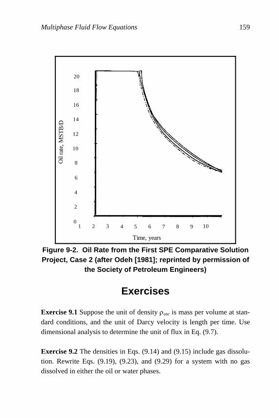
Multiphase Fluid Flow Equations 159
18
20
16
14
12
10
8
6
4
2
01 2 3 4 6 875 9 10
Time, years
Oil
r at e
,MST
B/D
Figure 9-2. Oil Rate from the First SPE Comparative Solution Project, Case 2 (after Odeh [1981]; reprinted by permission of
the Society of Petroleum Engineers)
Exercises Exercise 9.1 Suppose the unit of density ρosc is mass per volume at stan-
dard conditions, and the unit of Darcy velocity is length per time. Use dimensional analysis to determine the unit of flux in Eq. (9.7). Exercise 9.2 The densities in Eqs. (9.14) and (9.15) include gas dissolu-tion. Rewrite Eqs. (9.19), (9.23), and (9.29) for a system with no gas dissolved in either the oil or water phases.
160 Principles of Applied Reservoir Simulation
Exercise 9.3 Run EXAM3.DAT and record the time, pressure, oil rate, water rate, gas rate, and GOR at the end of the run. These values are ob-tained from the one line timestep summary file ITEMP.TSS. Is gas significant in this model? Note that the pressure reported for the reser-voir is pore volume weighted average reservoir pressure Pav. Pore volume weighted average reservoir pressure is given by
∑
∑
=
==N
jpj
N
jpjj
av
V
VP
P
1
1 (9.35)
where N is the total number of gridblocks in the model grid, Pj is the oil phase pressure in gridblock j, and Vpj is the pore volume of gridblock j. Exercise 9.4 Find the following properties in file EXAM8_PVTG.DAT: a. What is gas gravity? b. What is critical gas saturation? c. In which layer is well GAS1 completed? d. In which layer is well GAS2 completed? e. What is the size of the gridblock in the x direction? f. What is porosity in layer 1? g. What is permeability in the x, y and z directions in layer 2? Exercise 9.5 Find the following properties in file EXAM1.DAT: a. What is the net-to-gross ratio? b. What is residual oil saturation to a waterflood? c. What is the bubble point pressure? d. What is the depth to the midpoint of the gridblock? e. What is rock compressibility at bubble point pressure? f. Can any gas dissolve in water?
Exercise 9.6 A model has 10 × 10 × 4 gridblocks and takes five minutes to run 100 timesteps. Calculate cpu time per gridblock-timestep (GBTS).

Multiphase Fluid Flow Equations 161
Estimate how long it would take to make 100 runs with 200 timesteps each. Exercise 9.7 Data file EXAM7.DAT is one version of the Odeh [1981] SPE comparative solution problem. Run EXAM7.DAT and compare the oil rate to results reported by Odeh (see Figure 9-2). What is the IFLO material balance error? The material balance error associated with this data file provides a good test of the quality of IFLO relative to other pro-grams based on the original version of BOAST [for example, Fanchi, et al., 1982; Fanchi, et al., 1987; Louisiana State University, 1997]. Exercise 9.8A A reservoir is 10 mi. long and 4 mi. wide. Define a grid
with gridblock lengths ∆x = ∆y = 1/8 mi. What is the number of grid-blocks needed to cover the areal extent of the reservoir? Note: 1 mi. = 5280 ft. Exercise 9.8B If five model layers are used, what is the total number of gridblocks in the model?
162
Chapter 10
Fundamentals of Reservoir Simulation
Previous chapters describe much of the data that is needed by a reservoir simulator. Our goal here is to describe how the complex fluid flow equations presented in Chapter 9 are solved in practice. For a more detailed technical presentation, consult one of the many sources available in the literature [for example, see Aziz and Settari, 1979; Peaceman, 1977; Rosenberg, 1977; Thomas, 1982; Mattax and Dalton, 1990; Ertekin, et al., 2001; Munka and Pápay, 2001]. The technique used to solve the set of IFLO equations is presented as an illustration of a simu-lator solution procedure.
10.1 Simulator Solution Procedures Fluid flow equations are a set of nonlinear partial differential equations that must be solved by computer. The partial derivatives are replaced with finite differences, which are in turn derived from Taylor’s series. Table 10-1 outlines this procedure. The spatial finite difference
interval ∆x along the x-axis is called the gridblock length, and the tempo-
ral finite difference interval ∆t is called the timestep. Indices i, j, and k are ordinarily used to label grid locations along the x, y, and z coordinate axes, respectively. Index n labels the present time level, so that n+1

Fundamentals of Reservoir Simulation 163
represents a future time level. If the finite difference representations of the partial derivatives are substituted into the original flow equations, the result is a set of equations that can be algebraically rearranged to form a set of equations that can be solved numerically. The solution of these equations is the job of the simulator.
Table 10-1 Finite Difference Approximation
1. Formulate fluid flow equations, such as,
( ) ⎟⎠⎞
⎜⎝⎛ φ
∂∂
=−δ+⎥⎦
⎤⎢⎣
⎡⎟⎠⎞
⎜⎝⎛∂∂
µ∂∂
B
S
txxq
x
P
B
Kk
x sr
0
2. Approximate derivatives with finite differences
a. Discretize region into gridblocks ∆x:
x
P
xx
PP
x
P
ii
ii
∆∆
≡−−
≈∂∂
+
+
1
1
b. Discretize time into timesteps ∆t:
t
S
tt
SS
t
Snn
nn
∆∆
≡−−
≈∂∂
+
+
1
1
3. Numerically solve the resulting set of linear algebraic equations
The two most common solution procedures in use today are im-plicit pressure, explicit saturation (IMPES) and Newton-Raphson. The terms in the finite difference form of the flow equations are expanded in the Newton-Raphson procedure as the sum of each term at the current iteration level, plus a contribution due to a change of each term with re-spect to the primary unknown variables over the iteration. To calculate these changes, it is necessary to calculate derivatives, either numerically or analytically, of the flow equation terms. The derivatives are stored in a matrix called the acceleration matrix or the Jacobian. The Newton-
Raphson technique leads to a matrix equation RhXJ =• that equates
the product of the acceleration matrix J and a column vector hX of
changes to the primary unknown variables to the column vector of re-
siduals R . The matrix equation is solved by matrix algebra to yield the

164 Principles of Applied Reservoir Simulation
changes to the primary unknown variables hX . These changes are added
to the value of the primary unknown variables at the beginning of the iteration. If the changes are less than a specified tolerance, the iterative Newton-Raphson technique is considered complete and the simulator proceeds to the next timestep. The three primary unknown variables for an oil-water-gas sys-tem are oil-phase pressure, water saturation, and either gas saturation or solution gas-oil ratio. The choice of the third variable depends on whether the gridblock contains free gas, which depends, in turn, on whether the gridblock pressure is above or below the bubble point pres-sure. Naturally, the choice of unknowns is different for a gas-water system or a water only system. The discussion presented here applies to the most general three-phase case. The Newton-Raphson technique is known as a fully implicit technique because all primary variables are calculated at the same time; that is, primary variables at the new time level are determined simultane-ously. A simpler procedure is the IMplicit Pressure-Explicit Saturation (IMPES) procedure. It is much like the Newton-Raphson technique ex-cept that flow coefficients are not updated in an iterative process. By contrast, the IMPES procedure solves for pressure at the new time level using saturations at the old time level, and then uses the pressures at the new time level to explicitly calculate saturations at the new time level. A variation of this technique is to iteratively substitute the new time level estimates of primary variables in the calculation of coefficients for the flow equations. The iterative IMPES technique takes longer to run than the noniterative technique, but generates less material balance error [Ammer and Brummert, 1991]. IFLO, the program provided with this book, is an implementation of an iterative IMPES formulation. The for-mulation is outlined below. Figure 10-1 shows a flow chart for a typical simulator [see Crichlow, 1977]. The simulation program begins by reading input data and initializing the reservoir. This part of the model will not change as a function of time. Information for time-dependent data must then be read. This data includes well and field control data. The coefficients of the flow equations and the primary unknown variables are then calculated.

Fundamentals of Reservoir Simulation 165
Once the primary variables are determined, the process can be repeated by updating the flow coefficients using the values of the primary vari-ables at the new iteration level. This iterative process can improve material balance. When the solution of the fluid flow equations is com-plete, flow properties are updated and output files are created before the next timestep calculation begins.
Read Input
Initialize
Read Rates
Calculate Flow Coefficients
Solve Node Unknowns
Update Physical Properties
Create Output Files
START
END
Ne
w T
ime
Ste
p
IMPLICIT
IMPES
Figure 10-1. Typical simulator flow chart
Fully implicit techniques do more calculations in a timestep than the IMPES procedure, but are stable over longer timesteps. The uncondi-tional stability of the fully implicit techniques means that a fully implicit simulator can solve problems faster than IMPES techniques by taking significantly longer timesteps. Adaptive implicit techniques attempt to combine the best ele-ments of both IMPES and fully implicit techniques. An adaptive technique will use the IMPES method in regions of the model domain that have relatively small changes in primary variables, and apply the fully implicit method in regions that have relatively large changes in primary variables. Adaptive techniques can increase timestep size rela-tive to the IMPES method, and reduce computer resource requirements relative to the fully implicit method. Adaptive techniques use computer
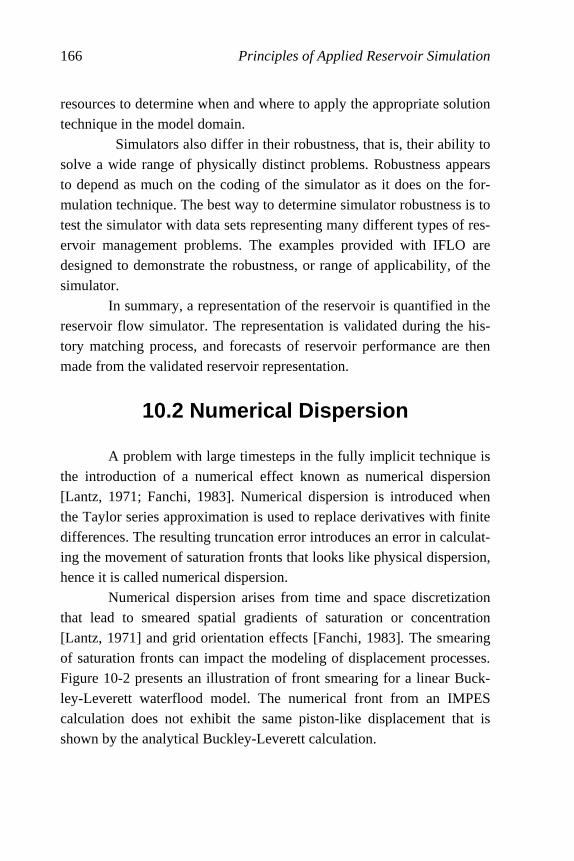
166 Principles of Applied Reservoir Simulation
resources to determine when and where to apply the appropriate solution technique in the model domain. Simulators also differ in their robustness, that is, their ability to solve a wide range of physically distinct problems. Robustness appears to depend as much on the coding of the simulator as it does on the for-mulation technique. The best way to determine simulator robustness is to test the simulator with data sets representing many different types of res-ervoir management problems. The examples provided with IFLO are designed to demonstrate the robustness, or range of applicability, of the simulator.
In summary, a representation of the reservoir is quantified in the reservoir flow simulator. The representation is validated during the his-tory matching process, and forecasts of reservoir performance are then made from the validated reservoir representation.
10.2 Numerical Dispersion A problem with large timesteps in the fully implicit technique is the introduction of a numerical effect known as numerical dispersion [Lantz, 1971; Fanchi, 1983]. Numerical dispersion is introduced when the Taylor series approximation is used to replace derivatives with finite differences. The resulting truncation error introduces an error in calculat-ing the movement of saturation fronts that looks like physical dispersion, hence it is called numerical dispersion. Numerical dispersion arises from time and space discretization that lead to smeared spatial gradients of saturation or concentration [Lantz, 1971] and grid orientation effects [Fanchi, 1983]. The smearing of saturation fronts can impact the modeling of displacement processes. Figure 10-2 presents an illustration of front smearing for a linear Buck-ley-Leverett waterflood model. The numerical front from an IMPES calculation does not exhibit the same piston-like displacement that is shown by the analytical Buckley-Leverett calculation.
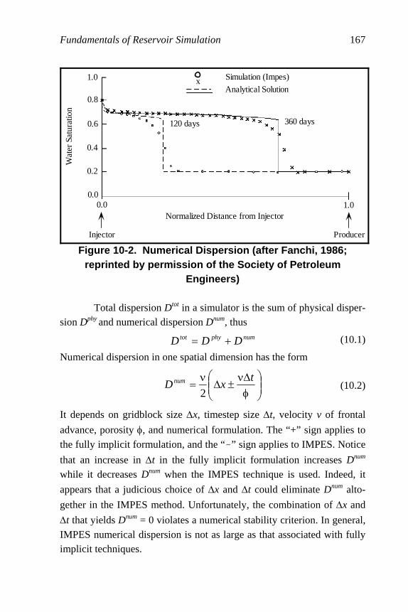
Fundamentals of Reservoir Simulation 167
Simulation (Impes)
Analytical Solutionx
360 days120 days
0.00.0
0.2
0.4
0.6
0.8
1.0
1.0
ProducerInjector
Wat
er S
atu
ratio
n
Normalized Distance from Injector
Figure 10-2. Numerical Dispersion (after Fanchi, 1986; reprinted by permission of the Society of Petroleum
Engineers)
Total dispersion Dtot in a simulator is the sum of physical disper-sion Dphy and numerical dispersion Dnum, thus
numphytot DDD += (10.1)
Numerical dispersion in one spatial dimension has the form
⎟⎟⎠
⎞⎜⎜⎝
⎛φ∆ν
±∆ν
=t
xDnum
2 (10.2)
It depends on gridblock size ∆x, timestep size ∆t, velocity v of frontal
advance, porosity φ, and numerical formulation. The “+” sign applies to
the fully implicit formulation, and the “-” sign applies to IMPES. Notice
that an increase in ∆t in the fully implicit formulation increases Dnum while it decreases Dnum when the IMPES technique is used. Indeed, it
appears that a judicious choice of ∆x and ∆t could eliminate Dnum alto-
gether in the IMPES method. Unfortunately, the combination of ∆x and
∆t that yields Dnum = 0 violates a numerical stability criterion. In general,
IMPES numerical dispersion is not as large as that associated with fully implicit techniques.
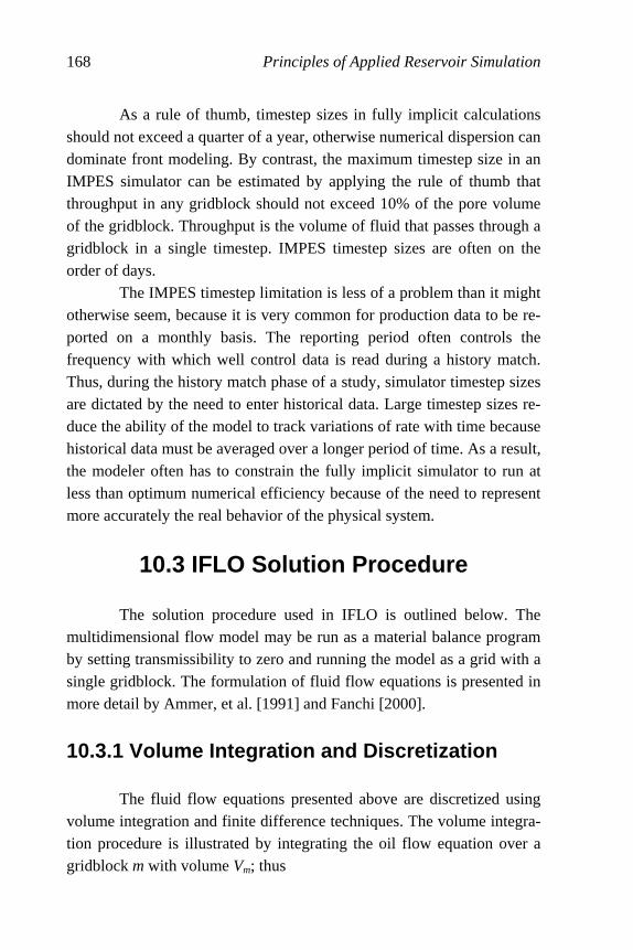
168 Principles of Applied Reservoir Simulation
As a rule of thumb, timestep sizes in fully implicit calculations should not exceed a quarter of a year, otherwise numerical dispersion can dominate front modeling. By contrast, the maximum timestep size in an IMPES simulator can be estimated by applying the rule of thumb that throughput in any gridblock should not exceed 10% of the pore volume of the gridblock. Throughput is the volume of fluid that passes through a gridblock in a single timestep. IMPES timestep sizes are often on the order of days. The IMPES timestep limitation is less of a problem than it might otherwise seem, because it is very common for production data to be re-ported on a monthly basis. The reporting period often controls the frequency with which well control data is read during a history match. Thus, during the history match phase of a study, simulator timestep sizes are dictated by the need to enter historical data. Large timestep sizes re-duce the ability of the model to track variations of rate with time because historical data must be averaged over a longer period of time. As a result, the modeler often has to constrain the fully implicit simulator to run at less than optimum numerical efficiency because of the need to represent more accurately the real behavior of the physical system.
10.3 IFLO Solution Procedure The solution procedure used in IFLO is outlined below. The multidimensional flow model may be run as a material balance program by setting transmissibility to zero and running the model as a grid with a single gridblock. The formulation of fluid flow equations is presented in more detail by Ammer, et al. [1991] and Fanchi [2000].
10.3.1 Volume Integration and Discretization
The fluid flow equations presented above are discretized using volume integration and finite difference techniques. The volume integra-tion procedure is illustrated by integrating the oil flow equation over a gridblock m with volume Vm; thus

Fundamentals of Reservoir Simulation 169
dVB
S
tdV
q
B
kK
mm V o
o
V osc
oo
oeo
ero ∫∫ ⎟⎟
⎠
⎞⎜⎜⎝
⎛φ
∂∂
=⎥⎦
⎤⎢⎣
⎡ρ
−Φ∇µ⋅∇ (10.3)
The divergence theorem is used to replace the volume integral over the convection term on the left hand side of Equation (10.3) with a surface integral. Applying the divergence theorem gives
dVB
S
tdV
qdSn
B
kK
mmem V o
o
V osc
o
S
oo
eo
ero ∫∫∫ ⎟⎟
⎠
⎞⎜⎜⎝
⎛φ
∂∂
=⎥⎦
⎤⎢⎣
⎡ρ
−⋅Φ∇µ
ˆ (10.4)
where gridblock volume Vm corresponds to the volume V, and the surface S is the external surface Sem of the gridblock m. The surface integral represents fluid flow across the gridblock boundaries. The spatially discretized material balance equation for oil is
oooo AQ
dt
dM∆Φ∆=+ (10.5)
where the volume integral over rate is
mosc
o
V osc
oo V
qdV
mρ
=ρ
= ∫ (10.6)
The volume integral over the accumulation term is
mo
o
V o
oo V
B
SdV
B
SM
m
φ=⎟⎟⎠
⎞⎜⎜⎝
⎛φ= ∫ (10.7)
and the surface integral is
∫ ⋅Φ∇µ
=∆Φ∆emS
oo
eo
ero
oo dSnB
kKA ˆ (10.8)
The term Ao represents oil phase transmissibility and oil phase potential is
DP no
nno γ∆−∆=∆Φ ++ 11 (10.9)
The variable P is oil phase pressure, D is depth to the center of the grid-
block, and γo is the specific gravity of the oil phase. The time derivative
in Equation (10.5) is replaced with a forward finite difference to obtain
170 Principles of Applied Reservoir Simulation
[ ] 11111 ++++ ∆Φ∆=+−∆
no
no
no
no
no AQMM
t(10.10)
The superscript n denotes the present time level tn, and the superscript n
+ 1 denotes the future time level tn+1. Timestep size ∆t equals tn+1 - tn.
The above formulation is a fully implicit formulation because all variables are assessed at the future time level in Equation (10.10). IMPES is invoked by approximating transmissibilities, capillary pres-sures and densities at time level n + 1 with their values at time level n. The resulting flow equation is
[ ] 1111 +++ ∆Φ∆=+−∆
no
no
no
no
no AQMM
t(10.11)
Similar equations apply to the other flow equations.
10.3.2 Multi-Variable Newton-Raphson IMPES Procedure
The IMPES equations developed above are solved using an it-erative technique that is illustrated by continuing our analysis of the oil flow equation. The residual form of Equation (10.11) is
[ ] llllo
noo
nooo AQMM
tR ∆Φ∆−+−
∆=
1(10.12)
where the superscript l denotes the iteration level for the variables that
are desired at time level n + 1. The primary variables for a saturated
gridblock are ∆P, ∆Sw, ∆Sg and {惟vi: I = 1, …, Ns}. Gas saturation is re-
placed by bubble point pressure Pb in the set of primary variables for a saturated gridblock. The variable switching logic used to treat gridblocks undergoing phase transitions is described in Ammer, et al. [1991]. The solution process is designed to find the values of the primary variables which drive the residuals to zero in all gridblocks for all components. Ammer, et al. [1991] refer to the solution procedure as the multivariable Newton-Raphson IMPES method.

Fundamentals of Reservoir Simulation 171
10.4 IFLO Transmissibility
Flow between neighboring gridblocks is treated as a series appli-cation of Darcy’s Law in IFLO. A transmissibility term between two gridblocks is defined using the product of average values of relative
permeability lrk of phase l , absolute permeability K of each gridblock
at the interface, and cross-sectional area cA of each gridblock at the in-
terface, divided by the product of the viscosity lµ of phase l and the
formation volume factor lB of phase l in each gridblock. The transmis-
sibility to each phase is determined using a harmonic average calculation of the product of absolute permeability times cross-sectional area at the interface between neighboring gridblocks. An arithmetic average of phase viscosities and formation volume factors is used. The average rela-tive permeability is determined using an upstream weighted averaging technique.
The Darcy transmissibility for the x-direction index i is
( )
( ) ( )( ) ( )
( ) ( ) ⎥⎦
⎤⎢⎣
⎡
∆+∆×
+µ+µ=′
−−
−
−−−
11
1
,1,,1,,
2
4
21
iciici
icic
iiii
upstreamr
i
KAxKAx
KAKA
BB
kA
llll
l
l
(10.13)
where the kj , indices are suppressed. The x-direction length of grid-
block i is ix∆ . The finite difference transmissibility for phase l
between gridblock 1−i and gridblock i is
⎟⎠⎞
⎜⎝⎛ ′′∆+′∆
∆′=−−
2
21
21 ,, xx
xAA i
ii ll
(10.14)
where the spatial differences are
iiii xxxxxx −=′′∆−=′∆ +− 11, (10.15)

172 Principles of Applied Reservoir Simulation
Similar definitions of transmissibility apply in all three coordinate direc-tions. Fully implicit formulations update relative permeability, viscos-ity, and formation volume factor as pressure and saturation distributions change during the iterative calculations that occur within a timestep. IMPES formulations update relative permeability, viscosity, and forma-tion volume factor using new pressure and saturation distributions following the completion of a timestep. Some simulators, such as IFLO, have options that let the user update permeability and cross-sectional area as functions of pressure and saturation. For example, cross-sectional area of gridblock i in Eq. (10.13) may be written as
( ) ( )inetiic zyA ∆∆= (10.16)
where iy∆ is the y-direction length of gridblock i and ( )inetz∆ is the net
thickness of gridblock i . The net thickness may shrink as a result of
compaction following a decrease in pore pressure. In addition, perme-ability may change as pore pressure changes. These effects have traditionally been neglected in black oil and compositional simulators, but are becoming more important as modelers recognize that geome-chanical effects are needed to understand the production performance of some reservoirs.
Flow simulators are usually programmed with no-flow boundary conditions, that is, fluid is not allowed to flow across the external boundaries of the grid. The no-flow boundary conditions are imposed by setting transmissibility equal to zero across the external boundaries. The user may also impose no-flow boundaries or flow restrictions across user-specified interfaces by directly modifying the appropriate transmis-sibility. This is useful, for example, when a geologic feature such as a sealing fault needs to be described. In this case, the sealing fault is de-fined by setting transmissibility equal to zero across the fault boundary. The user needs to understand how the transmissibility adjustment is made in a particular simulator because the transmissibility adjustment applies to the interface between rows, columns, or layers of gridblocks.

Fundamentals of Reservoir Simulation 173
10.5 IFLO Well Model A well model used in many simulators is a variation of Darcy’s Law which says that well flow rate is proportional to pressure change.
The relationship between flow rate lQ of phase l and pressure change
∆P may be written as
PPIQ ∆=l (10.17)
where the proportionality constant is called the productivity index (PI). Rearranging and using Darcy’s Law for radial flow into a vertical well-bore, PI can be calculated as
( )[ ]SrrB
hK
P
QPI
we
nete
+µ=
∆=
/ln
00708.0
ll
l (10.18)
The meaning and appropriate units of each variable in Eq. (10.18) fol-low:
lµ = viscosity of phase l (cp)
lB = formation volume factor of phase l (RB/STB)
re = drainage radius (ft)
rw = wellbore radius (ft)
S = skin
Ke = effective permeability (md) = absr Kk l
lrk = relative permeability of phase l
Kabs = absolute permeability (md)
hnet = net thickness (ft)
lQ = rate of phase l (STB/D)
Most flow simulators calculate PI and pressure change, then flow rate. If the magnitude of the flow rate calculated from the PI and

174 Principles of Applied Reservoir Simulation
pressure change is greater than the magnitude of the pressure change in-put by the user, the flow rate will usually be set at the user specified flow rate. If the magnitude of the flow rate calculated from the PI and pressure change is less than the magnitude of the pressure change input by the user, the flow rate will be the simulator calculated value. The reader should consult the technical documentation of a flow simulator to see the details of well model calculations. Well model features available in IFLO are described here.
10.5.1 IFLO Productivity Index Some of the terms in the PI depend on time-varying pressure and saturation, while other factors change relatively slowly or are constant with respect to time. Relative permeability, viscosity and formation vol-ume factor depend on time-varying pressure and saturation. The remaining variables on the right hand side of Eq. (10.18) change rela-tively slowly or are constant with respect to time. For example, we separate these terms for the oil phase PI to obtain
PIDB
kPI
oo
ro
µ= (10.19)
where the quasistationary factors are collected in the PID term, that is,
( )[ ]Srr
hKPID
we
netabs
+=
/ln
00708.0 (10.20)
The IFLO user is expected to provide a PID value for each well connec-tion. A connection is a gridblock with a well perforation.
A value of the effective drainage radius for a vertical well in the
center of a rectangular gridblock with cross-sectional area ∆x∆y can be estimated from Peaceman’s formula [1978]
( ) 21
22 yxrr oe ∆+∆=≈ 0.14 (10.21)
Equation (10.21) applies to an isotropic system, that is, a system in which lateral permeability does not depend on direction. For a well in a
square gridblock with isotropic permeability, we have yx ∆=∆ and
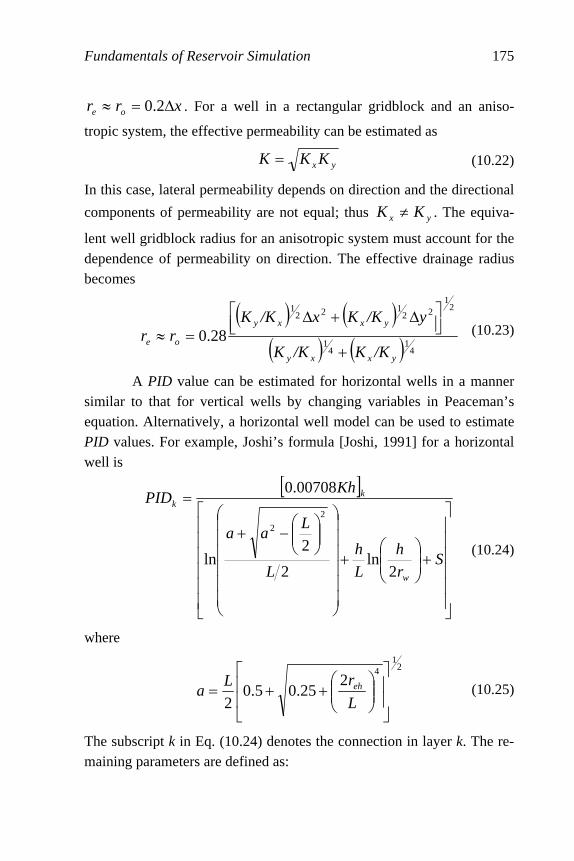
Fundamentals of Reservoir Simulation 175
xrr oe ∆=≈ 0.2 . For a well in a rectangular gridblock and an aniso-
tropic system, the effective permeability can be estimated as
yxKKK = (10.22)
In this case, lateral permeability depends on direction and the directional
components of permeability are not equal; thus yx KK ≠ . The equiva-
lent well gridblock radius for an anisotropic system must account for the dependence of permeability on direction. The effective drainage radius becomes
( ) ( )
( ) ( ) 41
41
21
22122
1
0.28yxxy
yxxy
oe/KK/KK
y/KKx/KKrr
+
⎥⎦⎤
⎢⎣⎡ ∆+∆
=≈ (10.23)
A PID value can be estimated for horizontal wells in a manner similar to that for vertical wells by changing variables in Peaceman’s equation. Alternatively, a horizontal well model can be used to estimate PID values. For example, Joshi’s formula [Joshi, 1991] for a horizontal well is
[ ]
⎥⎥⎥⎥⎥⎥
⎦
⎤
⎢⎢⎢⎢⎢⎢
⎣
⎡
+⎟⎟⎠
⎞⎜⎜⎝
⎛+
⎟⎟⎟⎟⎟⎟
⎠
⎞
⎜⎜⎜⎜⎜⎜
⎝
⎛
⎟⎟⎠
⎞⎜⎜⎝
⎛−+
=
Sr
h
L
h
L
Laa
KhPID
w
kk
2ln
2
2ln
00708.0
2
2
(10.24)
where
21
42
25.05.02 ⎥
⎥
⎦
⎤
⎢⎢
⎣
⎡
⎟⎟⎠
⎞⎜⎜⎝
⎛++=
L
rLa eh (10.25)
The subscript k in Eq. (10.24) denotes the connection in layer k. The re-maining parameters are defined as:

176 Principles of Applied Reservoir Simulation
K = horizontal permeability of connection k (md)
h = thickness of connection k (ft)
L = horizontal well length (ft)
reh = drainage radius of horizontal well (ft)
10.5.2 IFLO Rate Constraint Representation
In the rate constraint representation, well rates may be specified for injectors or producers. We assume the well may be completed in a total of K connections, and fluid allocation between connections is based on effective mobility そe and pressure differential 〉Pwk =P - Pwb between the pressure P in the gridblock containing the well connection and the user specified wellbore flowing pressure Pwb. Case 1: Pressure Differential for Specified Oil Production Rate Qo
The pressure differential for each connection k is
[ ] nko
eo
K
kk
owk
BPID
QP
λ=∆
∑=1
(10.26)
where elλ is the effective fluid mobility of phase l and PID is the well
productivity index. A PID may be specified for each connection k. Case 2: Pressure Differential for Specified Water Production Rate Qw The pressure differential for each connection k is
[ ] nkw
ew
K
kk
wwk
BPID
QP
λ=∆
∑=1
(10.27)
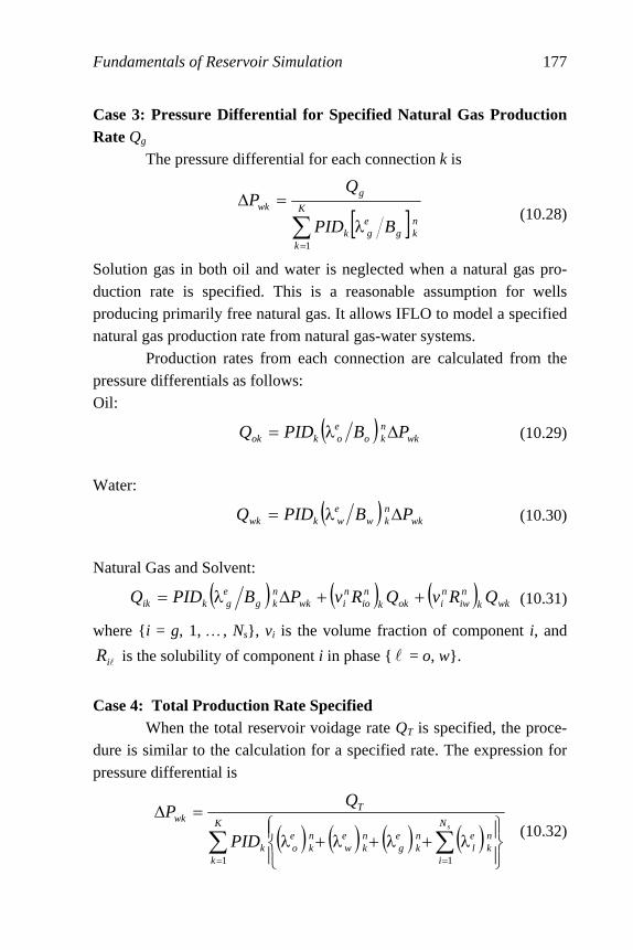
Fundamentals of Reservoir Simulation 177
Case 3: Pressure Differential for Specified Natural Gas Production Rate Qg The pressure differential for each connection k is
[ ] nkg
eg
K
kk
gwk
BPID
QP
λ=∆
∑=1
(10.28)
Solution gas in both oil and water is neglected when a natural gas pro-duction rate is specified. This is a reasonable assumption for wells producing primarily free natural gas. It allows IFLO to model a specified natural gas production rate from natural gas-water systems. Production rates from each connection are calculated from the pressure differentials as follows: Oil:
( ) wknko
eokok PBPIDQ ∆λ= (10.29)
Water:
( ) wknkw
ewkwk PBPIDQ ∆λ= (10.30)
Natural Gas and Solvent:
( ) ( ) ( ) wkkniw
niokk
nio
niwk
nkg
egkik QRvQRvPBPIDQ ++∆λ= (10.31)
where {i = g, 1, …, Ns}, vi is the volume fraction of component i, and
liR is the solubility of component i in phase {l = o, w}.
Case 4: Total Production Rate Specified When the total reservoir voidage rate QT is specified, the proce-dure is similar to the calculation for a specified rate. The expression for pressure differential is
( ) ( ) ( ) ( )⎪⎭
⎪⎬⎫
⎪⎩
⎪⎨⎧
λ+λ+λ+λ
=∆
∑∑==
sN
i
nk
el
nk
eg
nk
ew
nk
eo
K
kk
Twk
PID
QP
11
(10.32)

178 Principles of Applied Reservoir Simulation
The pressure differential is then used in the rate equations, Eqs. (10.29) through (10.31), to calculate rates. Case 5: Injection Rate Specified If the well is an injector, the user must specify the surface injec-tion rate Qi of component i and a well injectivity index WIk for each connection. The components that may be injected are water, natural gas, and solvent. The injection rate for each connection is then allocated us-ing the following formulas.
Component {i = w, g, 1, …, Ns} Injection Pressure Differential:
( ) ( ) ( ) ( )⎪⎭
⎪⎬⎫
⎪⎩
⎪⎨⎧
λ+λ+λ+λ
=∆
∑∑==
sN
i
nk
el
nk
eg
nk
ew
nk
eo
K
knik
k
iwk
B
WI
QP
11
(10.33)
Component {i = w, g, 1, …, Ns} Injection Rate:
( ) ( ) ( ) ( )⎥⎥⎦
⎤
⎢⎢⎣
⎡λ+λ+λ+λ
∆= ∑
=
sN
i
nk
el
nk
eg
nk
ew
nk
eon
ik
wkkik B
PWIQ
1
(10.34)
Allocation of injection fluids is based on total mobilities.
10.5.3 Explicit Pressure Constraint Representation
In the explicit pressure constraint representation, pressure differ-entials are used to calculate flow rates for injectors or producers. Case 1: Explicit Pressure Constrained Well The pressure differential for explicit pressure specified wells is given by
kwbn
wk PPP ][ −=∆ (10.35)
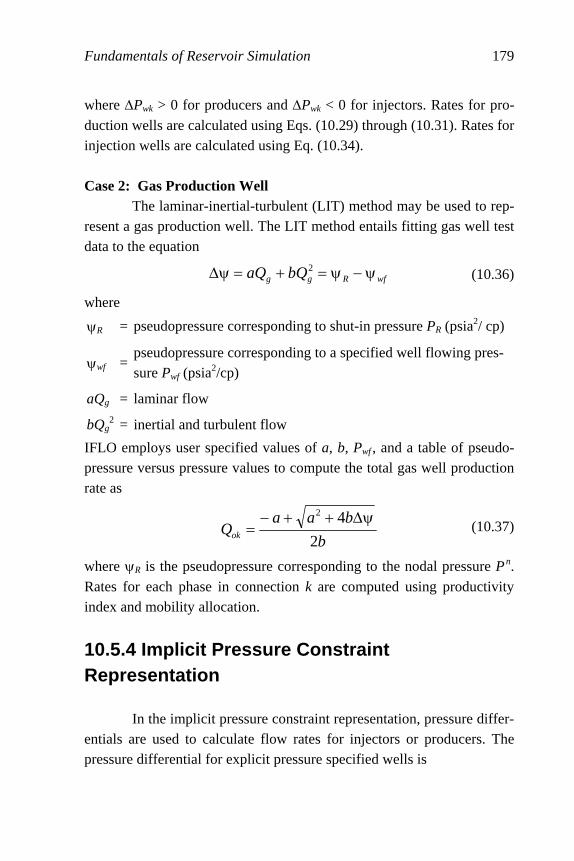
Fundamentals of Reservoir Simulation 179
where ∆Pwk > 0 for producers and ∆Pwk < 0 for injectors. Rates for pro-
duction wells are calculated using Eqs. (10.29) through (10.31). Rates for injection wells are calculated using Eq. (10.34). Case 2: Gas Production Well The laminar-inertial-turbulent (LIT) method may be used to rep-resent a gas production well. The LIT method entails fitting gas well test data to the equation
wfRgg bQaQ ψ−ψ=+=ψ∆ 2 (10.36)
where
ψR = pseudopressure corresponding to shut-in pressure PR (psia2/ cp)
ψwf = pseudopressure corresponding to a specified well flowing pres-sure Pwf (psia2/cp)
aQg = laminar flow
bQg2 = inertial and turbulent flow
IFLO employs user specified values of a, b, Pwf, and a table of pseudo-pressure versus pressure values to compute the total gas well production rate as
b
baaQok 2
42 ψ∆++−= (10.37)
where ψR is the pseudopressure corresponding to the nodal pressure Pn.
Rates for each phase in connection k are computed using productivity index and mobility allocation.
10.5.4 Implicit Pressure Constraint Representation
In the implicit pressure constraint representation, pressure differ-entials are used to calculate flow rates for injectors or producers. The pressure differential for explicit pressure specified wells is

180 Principles of Applied Reservoir Simulation
kwbn
wk pPP ][ 1 −=∆ + (10.38)
where ∆Pwk > 0 for producers and ∆Pwk < 0 for injectors. The implicit
pressure constraint representation differs from the explicit pressure rep-
resentation by the use of the pressure 1+nP for the future time. This pressure must be included in the matrix equations that are solved implic-
itly for pressure. When 1+nP is known, rates for production wells are calculated using Eqs. (10.29) through (10.31), and rates for injection wells are calculated using Eq. (10.34).
10.5.5 Gas-Oil Ratio and Water-Oil Ratio Constraints Maximum gas-oil ratio (GORmax) and maximum water-oil ratio (WORmax) can be entered by the user for each oil production well. The gas-oil ratio (GOR) for a well is defined as total gas production for all active well completion intervals during the timestep divided by total oil production for all active well completion intervals during the timestep. If GOR for the well exceeds GORmax, then the completion interval (connec-tion) with the highest GOR will be shut in. The procedure is repeated until GOR is less than GORmax or until the well is shut in. The water-oil ratio (WOR) is defined as total water production for all active well completion intervals during the timestep divided by total oil production for all active well completion intervals during the timestep. If WOR for the well exceeds WORmax, then the completion interval (connection) with the highest WOR will be shut in. The proce-dure is repeated until WOR is less than WORmax or until the well is shut in.
10.5.6 Fluid Withdrawal Constraints Fluid withdrawal from explicit pressure controlled production wells can be constrained for primary phases as follows: A. A minimum production rate QWMIN can be specified.

Fundamentals of Reservoir Simulation 181
B. A maximum production rate QWMAX can be specified. Primary phases subject to fluid production constraints are oil, water, natural gas, and total fluid. A positive value of QWMIN for a pressure controlled production well is used as the minimum allowed production rate. If the calculated primary phase production rate drops below the minimum allowed value, the well is shut in. A positive value of QWMAX for a pressure controlled produc-tion well is used as the maximum allowed primary phase production rate. If the calculated primary phase production rate exceeds the maximum allowed value, calculated production will be reduced to the allowed value. Production from each connection is proportionally reduced by the ratio of allowed to calculated primary phase production rates.
10.5.7 Fluid Injection Constraints Fluid injection using explicit pressure controlled injection wells can be constrained for primary phases as follows: A. A minimum injection rate QWMIN can be specified. B. A maximum injection rate QWMAX can be specified. Primary phases subject to fluid injection constraints are water and natural gas. A negative value of QWMIN for a pressure controlled injection well is used as the minimum allowed injection rate. If the absolute value of the calculated primary phase injection rate drops below the absolute value of the minimum allowed injection rate, the well is shut in. A negative value of QWMAX for a pressure controlled injection well is used as the maximum allowed primary phase injection rate. If the absolute value of the calculated primary phase injection rate exceeds the absolute value of the maximum allowed injection rate, calculated injec-tion will be reduced to the allowed value. Injection from each connection is proportionally reduced by the ratio of the absolute values of allowed to calculated injection rates.
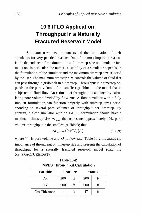
182 Principles of Applied Reservoir Simulation
10.6 IFLO Application: Throughput in a Naturally Fractured Reservoir Model
Simulator users need to understand the formulation of their simulators for very practical reasons. One of the most important reasons is the dependence of maximum allowed timestep size on simulator for-mulation. In particular, the numerical stability of a simulator depends on the formulation of the simulator and the maximum timestep size selected by the user. The maximum timestep size controls the volume of fluid that can pass through a gridblock in a timestep. Throughput in a timestep de-pends on the pore volume of the smallest gridblock in the model that is subjected to fluid flow. An estimate of throughput is obtained by calcu-lating pore volume divided by flow rate. A flow simulator with a fully implicit formulation can function properly with timestep sizes corre-sponding to several pore volumes of throughput per timestep. By contrast, a flow simulator with an IMPES formulation should have a
maximum timestep size maxt∆ that represents approximately 10% pore
volume throughput in the smallest gridblock; thus
( ) QVt P10.0max =∆ (10.39)
where PV is pore volume and Q is flow rate. Table 10-2 illustrates the
importance of throughput on timestep size and presents the calculation of throughput for a naturally fractured reservoir model (data file XS_FRACTURE.DAT).
Table 10-2 IMPES Throughput Calculation
Variable Fracture Matrix
DX 200 ft 200 ft
DY 600 ft 600 ft
Net Thickness 1 ft 47 ft

Fundamentals of Reservoir Simulation 183
Porosity 0.01 0.25
10% Pore Volume 21.4 RB 25100 RB
Flow Rate 100 STB/D 100 STB/D
Oil FVF 1.47 RB/STB 1.47 RB/STB
〉tmax 0.3 days 369 days
According to the data presented in Table 10-2, the maximum
timestep size calculated from Eq. (10.39) for a fracture gridblock is much smaller than the maximum timestep size calculated for a matrix gridblock. This is typical of naturally fractured reservoir models. One of the motivations for developing fully implicit flow models was to devise a formulation that did not have the maximum timestep size limitation as-sociated with the IMPES formulation.
The value of 〉tmax for the fracture gridblock is the value that should be used in the flow model. If a value of 〉tmax greater than the fracture 〉tmax is used in the flow model, the model can experience nu-merical difficulties such as oscillations in flow rates or unacceptable material balance errors. The result of using 〉tmax = 3 days in XS_FRACTURE.DAT leads to the numerical oscillations in water pro-duction rate shown in Figure 10-3. This figure should be compared with Figure 6-7, which is the result of using 〉tmax = .03 days. The rate spike in the first 50 days of Figure 10-3 is an example of model instability, and the abrupt fluctuations in rate shown throughout the simulation period are examples of numerical oscillations. If 〉tmax in the model is less than fracture 〉tmax, the rate fluctuations in Figure 10-3 will disappear (see Figure 6-7).

184 Principles of Applied Reservoir Simulation
Figure 10-3. Example of Numerical Oscillations
Exercises
Exercise 10.1 Reorder the following steps for a Typical Simulator Flow-chart. Note: Disregard any iterative looping in the ordering process. A. Calculate Flow Coefficients Step 1. B. Create Output Files Step 2. C. Initialize Step 3. D. Solve Node Unknowns Step 4. E. Read Rates Step 5. F. Update Physical Properties Step 6. G. Read Input Step 7.
Exercise 10.2 Data file EXAM3.DAT can be used to study the numeri-cal dispersion associated with a Buckley-Leverett type waterflood of an undersaturated oil reservoir. Run EXAM3.DAT with constant timesteps of 5 days, 10 days, and 15 days. Plot water saturation (vertical axis) ver-sus x-direction gridblock index I (horizontal axis) at 365 days. Note: you
0
200
400
600
800
1000
1200
1400
0 50 100 150 200 250 300 350 400
Time (days)
Water Production Rate
Fundamentals of Reservoir Simulation 185
will have to change the time reports are written to a single report at 365 days and set the maximum time of the run to 365 days. Exercise 10.3 File GOM_UNCONSOLIDATED.DAT represents oil production from a reservoir with properties analogous to an unconsoli-dated formation in the Gulf of Mexico. For comparison, data file GOM_UNCONSOLIDATED_TRANS.DAT allows permeability and cross-sectional area in the transmissibility calculation to change as pres-sure and saturation change. Run both files and make the following plots: pore volume weighted average reservoir pressure versus time; oil pro-duction rate versus time; cumulative oil production versus time; water production rate versus time; and cumulative water production versus time. Where do the greatest differences appear? Exercise 10.4 List at least two differences between IMPES and the fully implicit technique. Exercise 10.5 Data file VFILL3_WF.DAT illustrates the use of well controls in IFLO. Run VFILL3_WF.DAT and rerun it using an oil rate of 150 STBPD. How long do both models run? Exercise 10.6 Data file EXAM9_LIT.DAT has a gas well under LIT control. Determine the effect of doubling the turbulence factor on reser-voir pressure, gas production rate from layers 1 and 2, and water production rate from layer 2 for the LIT controlled gas well. Exercise 10.7A Suppose gridblock length is 100 ft, velocity of frontal advance is 0.5 ft/day, porosity is 0.2, and timestep size is 30 days. Use Lantz’s expression for numerical dispersion to calculate numerical dis-persion for both IMPES and fully implicit reservoir simulator formulations. Exercise 10.7B If water is displacing oil, will water breakthrough occur sooner in an IMPES or a fully implicit model based on the data given above? Why?

186 Principles of Applied Reservoir Simulation
Exercise 10.8 Place the wells in the 9 × 9 grid below using the following
well data:
Well I J Depth (ft)
W1 3 2 1200
W2 7 3 1220
W3 2 6 1180
W4 6 8 1190
I:1 2 3 4 5 6 7 8 9
J:1
2
3
4
5
6
7
8
9
Exercise 10.9A Data file XS_FRACTURE.DAT is a model of a natu-rally fractured reservoir. Most of the flow in this model is through the fractures. Run XS_FRACTURE.DAT and report the cumulative material balance errors for oil, water and gas at the end of the run. Exercise 10.9B Multiply the maximum timestep in data file XS_FRACTURE.DAT by a factor of ten and run the revised data file. Verify Figure 10-3 and report the cumulative material balance errors for oil, water and gas at the end of the run. Compare the material balance errors from Part B with the material balance errors found in Part A and explain your results.
187
Chapter 11
Overview of the Modeling Process
The best technology for making reservoir performance predic-tions today is to model fluid flow in porous media using reservoir flow simulators. The reservoir management process and the systems involved in reservoir modeling are outlined here.
11.1 Prerequisites Several prerequisites should be satisfied before a model study is undertaken [Coats, 1969]. The most important, from a business perspec-tive, is establishing that the problem has economic importance. At the very least, the objectives of a model study should yield a solution to the economically important problem. Once the objectives of a study are specified, the modeling team should gather all available data and reports relating to the field. Reser-voir characterization and reservoir engineering evaluations are usually performed as standard business practice. Some of the tasks associated with basic reservoir analysis are described in Chapter 2. They provide information that is needed to prepare input data for a simulation study. For example, material balance studies require the acquisition of fluid property data, field pressures, and production volumes. This information
188 Principles of Applied Reservoir Simulation
is also needed to conduct a flow model study. Volumetric analyses pro-vide independent appraisals of reservoir volume that can be used to check the original fluid volumes calculated by a reservoir flow model. In addition, basic reservoir analysis can provide an initial concept of the reservoir and associated drive mechanisms. These concepts can be used to design the model study. The modeling team needs to be aware of ex-isting studies and should relate model performance to previous studies whenever possible.
If data that are needed for the flow model are not available, the modeling team should determine if the data can be obtained, either by analogy with other reservoirs or by correlation. Values for all model in-put data must be obtained because the simulator will not run without a complete set of data. In some cases, it may be necessary to make simpli-fying assumptions about the reservoir because there is not enough data available to represent the system in greater quantitative detail. In addition to clearly defined objectives, another prerequisite that must be satisfied before committing to a simulation study is the de-termination that the objectives of the study cannot be achieved using simpler techniques. If less expensive techniques, such as decline curve analysis or the Buckley-Leverett waterflood displacement algorithm, do not provide adequate results, then more sophisticated and costly methods are justified.
11.2 Major Elements of a Reservoir Simulation Study
The essential elements of a simulation study include matching field history; making predictions, including a forecast based on the exist-ing operating strategy; and evaluating alternative operating scenarios [see, for example, Carlson, 2003; and Ertekin, et al., 2001]. We assume that a decision has been made to conduct a reservoir simulation study and that all relevant data has been acquired. The first phase of the reser-voir simulation study is the history matching phase.

Overview of the Modeling Process 189
History matching is an iterative process that makes it possible to integrate reservoir geoscience and engineering data. History matching is also referred to as model calibration in the literature [Aziz, et al., 2002] because the modeling team should verify and refine the reservoir de-scription during the history match, or model calibration, process. Starting with an initial reservoir description, the model is used to match and pre-dict reservoir performance. If necessary, the modeling team will modify the reservoir description until an acceptable match is obtained. The history matching process may be considered an inverse problem because an answer already exists. We know how the reservoir performed; we want to understand why. Our task is to find the set of res-ervoir parameters that minimizes the difference between the model performance and the historical performance of the field. This is a non-unique problem since there is usually more than one way to match the available data. Once a match of historical data is available, the next step is to make a base case prediction, which is essentially just a continuation of existing operating practice. The base case prediction gives a baseline for comparison with other reservoir management strategies. Model users should be aware of the validity of model predic-tions. One way to get an idea of the accuracy of predictions is to measure the success of forecasts made in the past. Lynch [1996] looked at the evolution of the United States Department of Energy price forecast over a period of several years for both oil and gas. Lynch’s study showed that there is considerable uncertainty associated with the price forecast. The variation in oil price by a factor of two in the late 1990's illustrates the volatility of economic factors that are needed in cash flow forecasts. In addition to uncertainty in economic parameters, there is un-certainty in the forecasted production performance of a field. Forecasts do not account for discontinuities in historical patterns that arise from unexpected effects. This is as true in the physical world as it is in the social [Oreskes, et al., 1994]. Simulators do not eliminate uncertainty; they give us the ability to assess and better manage the risk associated with the prediction of production performance.
190 Principles of Applied Reservoir Simulation
A valuable but intangible benefit of the process associated with reservoir simulation is the help it provides in managing the reservoir. One of the critical tasks of reservoir management is the acquisition and maintenance of an up-to-date data base. A simulation study can help co-ordinate activities as a modeling team gathers the resources it needs to determine the optimum plan for operating a field. Collecting input data for a model is a good way to ensure that every important technical vari-able is considered as data is collected from the many disciplines that contribute to reservoir management. If model performance is especially sensitive to a particular parameter, then a plan should be made to deter-mine that parameter more accurately, for example, from either laboratory or appropriate field tests.
11.3 Reservoir Management Modeling System
A comprehensive reservoir management modeling system can be thought of as four interacting subsystems: the reservoir model, the well model, the wellbore model, and the surface model. Figure 11-1 illustrates the spatial relationship between these models.
Every practical reservoir simulator includes both a reservoir model and a well model. The reservoir model represents fluid flow within the reservoir. The well model is a term in the fluid flow equations that represents the extraction of fluids from the reservoir or the injection of fluids into the reservoir. Full featured commercial simulators also in-clude a wellbore model and a surface facility model. The wellbore model represents flow from the sandface to the surface. The surface model represents constraints associated with surface facilities, such as platform and separator limitations. The mathematical algorithms associated with each model depend on physical conservation laws and empirical relationships. Computer simulators are based on conservation of mass, momentum, and energy. The most widely used simulators assume the reservoir is isothermal, that is, maintains a constant temperature. If we are modeling a reservoir
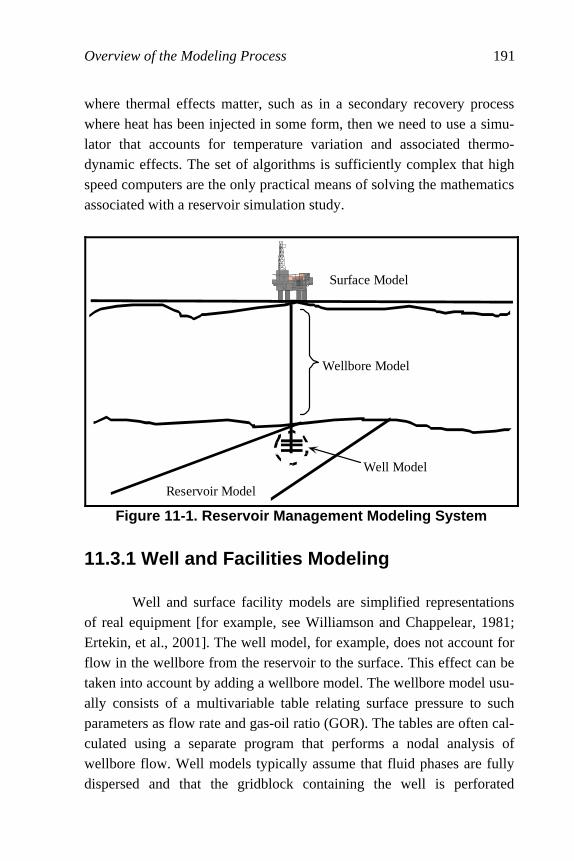
Overview of the Modeling Process 191
where thermal effects matter, such as in a secondary recovery process where heat has been injected in some form, then we need to use a simu-lator that accounts for temperature variation and associated thermo-dynamic effects. The set of algorithms is sufficiently complex that high speed computers are the only practical means of solving the mathematics associated with a reservoir simulation study.
Surface Model
Wellbore Model
Well Model
Reservoir Model
Figure 11-1. Reservoir Management Modeling System
11.3.1 Well and Facilities Modeling Well and surface facility models are simplified representations of real equipment [for example, see Williamson and Chappelear, 1981; Ertekin, et al., 2001]. The well model, for example, does not account for flow in the wellbore from the reservoir to the surface. This effect can be taken into account by adding a wellbore model. The wellbore model usu-ally consists of a multivariable table relating surface pressure to such parameters as flow rate and gas-oil ratio (GOR). The tables are often cal-culated using a separate program that performs a nodal analysis of wellbore flow. Well models typically assume that fluid phases are fully dispersed and that the gridblock containing the well is perforated

192 Principles of Applied Reservoir Simulation
throughout its thickness. Some commercial simulators will let the user specify a perforation interval under certain conditions. The different types of well controls include production and in-jection well controls, and group and field controls for a surface model. The production well model assumes the user specifies one option as the primary control, but may also specify other options as targets for con-straining the primary control. For example, if oil rate is the primary control, then the produced GOR may be restricted so that the oil rate is decreased when GOR exceeds a specified value. This provides a more realistic representation of actual field practice. Injection well controls assume that initial injection well mobility is given by total gridblock mobility. This makes it possible to inject a phase into a gridblock that would otherwise have zero relative perme-ability to flow. Allocation of fluids in a well model depends on layer flow ca-pacity and fluid mobility. Simulators can also describe deviated or horizontal wells depending on how the well completions and parameters are specified. Well, group and field controls can be specified in commercial simulators with a surface facilities model. The user specifies a hierarchy of controls that most realistically represent how the field is being oper-ated. For example, well production may be constrained by platform separator and storage capacity, which in turn is constrained by pipeline flow capacity. The ability to integrate reservoir and surface flow tech-nology using a single simulator is an area of research that is receiving increasing attention [for example, see Heinemann, et al., 1998].
11.4 Wellbore Modeling
The well model may be coupled to a wellbore model to more ac-curately account for fluid flow in pipes. Figure 11-2 illustrates the system of interest. The purpose of this section is to discuss the coupling of well models with wellbore models. We begin with a description of the physical phenomena, and then discuss simulation technology.
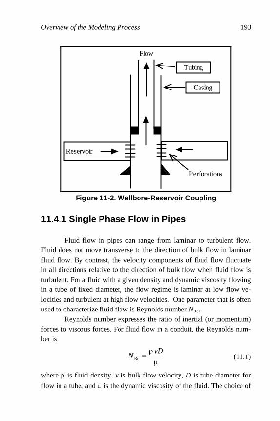
Overview of the Modeling Process 193
Reservoir
Flow
Tubing
Casing
Perforations
Figure 11-2. Wellbore-Reservoir Coupling
11.4.1 Single Phase Flow in Pipes
Fluid flow in pipes can range from laminar to turbulent flow. Fluid does not move transverse to the direction of bulk flow in laminar fluid flow. By contrast, the velocity components of fluid flow fluctuate in all directions relative to the direction of bulk flow when fluid flow is turbulent. For a fluid with a given density and dynamic viscosity flowing in a tube of fixed diameter, the flow regime is laminar at low flow ve-locities and turbulent at high flow velocities. One parameter that is often used to characterize fluid flow is Reynolds number NRe.
Reynolds number expresses the ratio of inertial (or momentum) forces to viscous forces. For fluid flow in a conduit, the Reynolds num-ber is
µ
ρ=
vDNRe (11.1)
where ρ is fluid density, v is bulk flow velocity, D is tube diameter for
flow in a tube, and µ is the dynamic viscosity of the fluid. The choice of

194 Principles of Applied Reservoir Simulation
units must yield a dimensionless Reynolds number. In System Interna-
tionale (SI) units, a dimensionless Reynolds number is obtained if fluid density is in kg/m3, flow velocity is in m/s, tube diameter is in m, and dynamic viscosity is in Pa·s. Note that 1 cp = 1 mPa·s = 10-3 Pa·s.
We introduce the factors that influence fluid flow in pipe by con-sidering the relatively simple case of single-phase flow in circular pipes [Beggs, 1991; Brill and Mukherjee, 1999]. Laminar flow along the longi-tudinal axis of a circular pipe is transverse to the cross-sectional area of the pipe. The cross-sectional area A of a circular pipe with internal radius r and internal diameter D is
2
22 ⎟
⎠⎞
⎜⎝⎛π=π=
DrA (11.2)
The bulk flow velocity v of a single-phase fluid flowing in the circular pipe is related to volumetric flow rate q by
24
D
q
A
qv
π== (11.3)
The Reynolds number for flow in a circular pipe can be written in terms of volumetric flow rate by substituting Equation (11.3) into (11.1) to give
D
qvDN
πµρ
=µ
ρ=
4Re (11.4)
where ρ is fluid density and µ is the dynamic viscosity of the fluid. Fluid
flow in circular pipes is laminar if NRe < 2000, and it is considered turbu-lent at larger values of the Reynolds number. The relationship between fluid flow velocity and pressure change along the longitudinal axis of the circular pipe is obtained by per-forming an energy balance calculation. Figure 11-3 shows the geometry of an inclined circular pipe with length L along the longitudinal axis and
angle of inclination θ. The single-phase fluid has density ρ and dynamic
viscosity µ. It is flowing in a gravity field with acceleration g.

Overview of the Modeling Process 195
AL
v
θ
Figure 11-3. Flow in an Inclined Circular Pipe
We make two simplifying assumptions in our analysis that allow
us to minimize external factors and consider only mechanical energy terms. We assume that no heat energy is added to the fluid, and that no work is done on the system by its surroundings, e.g. no mechanical de-vices such as pumps or compressors are adding energy to the system. An energy balance with these assumptions yields the pressure gradient equa-tion
fricKEPE dL
dP
dL
dP
dL
dP
dL
dP⎥⎦⎤
⎢⎣⎡+⎥⎦
⎤⎢⎣⎡+⎥⎦
⎤⎢⎣⎡= (11.5)
where P is pressure. We have written the pressure gradient along the longitudinal axis of the pipe as the sum of a potential energy term
θρ=⎥⎦⎤
⎢⎣⎡
singdL
dP
PE
(11.6)
a kinetic energy term
dL
dvv
dL
dP
KE
ρ=⎥⎦
⎤⎢⎣
⎡ (11.7)
and a friction term
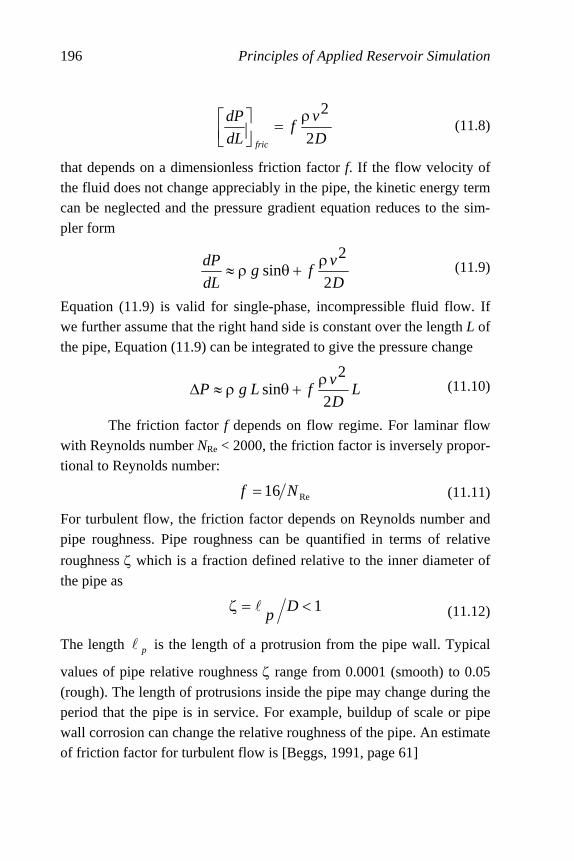
196 Principles of Applied Reservoir Simulation
D
vf
dL
dP
fric 2
2ρ=⎥⎦
⎤⎢⎣⎡
(11.8)
that depends on a dimensionless friction factor f. If the flow velocity of the fluid does not change appreciably in the pipe, the kinetic energy term can be neglected and the pressure gradient equation reduces to the sim-pler form
D
vfg
dL
dP
2
2sin
ρ+θρ≈ (11.9)
Equation (11.9) is valid for single-phase, incompressible fluid flow. If we further assume that the right hand side is constant over the length L of the pipe, Equation (11.9) can be integrated to give the pressure change
LD
vfLgP
2
2sin
ρ+θρ≈∆ (11.10)
The friction factor f depends on flow regime. For laminar flow with Reynolds number NRe < 2000, the friction factor is inversely propor-tional to Reynolds number:
Re16 Nf = (11.11)
For turbulent flow, the friction factor depends on Reynolds number and pipe roughness. Pipe roughness can be quantified in terms of relative
roughness ζ which is a fraction defined relative to the inner diameter of the pipe as
1<=ζ Dp
l (11.12)
The length pl is the length of a protrusion from the pipe wall. Typical
values of pipe relative roughness ζ range from 0.0001 (smooth) to 0.05 (rough). The length of protrusions inside the pipe may change during the period that the pipe is in service. For example, buildup of scale or pipe wall corrosion can change the relative roughness of the pipe. An estimate of friction factor for turbulent flow is [Beggs, 1991, page 61]
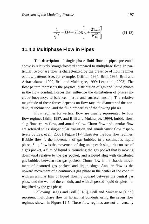
Overview of the Modeling Process 197
⎥⎥⎦
⎤
⎢⎢⎣
⎡+ζ−=
9.0Re
2521log2141
1
N
..
f (11.13)
11.4.2 Multiphase Flow in Pipes
The description of single phase fluid flow in pipes presented above is relatively straightforward compared to multiphase flow. In par-ticular, two-phase flow is characterized by the presence of flow regimes or flow patterns [see, for example, Griffith, 1984; Brill, 1987; Brill and Arirachakaran, 1992; Brill and Mukherjee, 1999; Lea, et al., 2003]. The flow pattern represents the physical distribution of gas and liquid phases in the flow conduit. Forces that influence the distribution of phases in-clude buoyancy, turbulence, inertia and surface tension. The relative magnitude of these forces depends on flow rate, the diameter of the con-duit, its inclination, and the fluid properties of the flowing phases.
Flow regimes for vertical flow are usually represented by four flow regimes [Brill, 1987; and Brill and Mukherjee, 1999]: bubble flow, slug flow, churn flow, and annular flow. Churn flow and annular flow are referred to as slug-annular transition and annular-mist flow respec-tively by Lea, et al. [2003]. Figure 11-4 illustrates the four flow regimes. Bubble flow is the movement of gas bubbles in a continuous liquid phase. Slug flow is the movement of slug units; each slug unit consists of a gas pocket, a film of liquid surrounding the gas pocket that is moving downward relative to the gas pocket, and a liquid slug with distributed gas bubbles between two gas pockets. Churn flow is the chaotic move-ment of distorted gas pockets and liquid slugs. Annular flow is the upward movement of a continuous gas phase in the center of the conduit with an annular film of liquid flowing upward between the central gas phase and the wall of the conduit, and with dispersed liquid droplets be-ing lifted by the gas phase.
Following Beggs and Brill [1973], Brill and Mukherjee [1999] represent multiphase flow in horizontal conduits using the seven flow regimes shown in Figure 11-5. These flow regimes are not universally

198 Principles of Applied Reservoir Simulation
accepted. For example, Brill and Arirachakaran [1992] used a similar set of flow regimes that were organized in terms of stratified flow, intermit-tent flow, annular flow, and dispersed bubble flow. More recently, Petalas and Aziz [2000] used the following set of flow regimes to repre-sent multiphase flow in pipes: dispersed bubble flow, stratified flow, annular-mist flow, bubble flow, intermittent flow, and froth flow. Froth flow was described as a transition zone between dispersed bubble flow and annular-mist flow, and between annular-mist flow and slug flow.
BubbleFlow
SlugFlow
ChurnFlow
AnnularFlow
Figure 11-4. Flow regimes for vertical, two-phase flow
(adapted from Brill and Mukherjee [1999, Figure 4.21 and AIChE])
Segregated
Stratified
Wavy
Annular
Intermittent
Distributed
Plug
Slug
Bubble
Mist
Figure 11-5. Flow regimes for horizontal, two-phase flow (adapted from Brill and Mukherjee [1999, Figure 4.16])

Overview of the Modeling Process 199
11.4.3 Modeling Multiphase Flow in Pipes The identification of qualitative flow regimes discussed above influences the structure of analytical and numerical models used to quan-tify multiphase flow in conduits. The flow regimes are used to construct flow regime maps, also called flow pattern maps, which are log-log plots of superficial gas velocity versus superficial liquid velocity. Figure 11-6 illustrates a flow pattern map.
Dispersed Bubble
IntermittentAnnular
StratifiedSmooth
StratifiedWavy
SuperficialLiquid
Velocity
Superficial Gas Velocity
Figure 11-6. Illustration of a flow pattern map (adapted from Brill and Arirachakaran [1992, Figure 2] )
Historically, predictions of multiphase flow in pipes began in the 1950’s when investigators used data from laboratory test facilities and, to a lesser extent, field data to prepare empirical flow pattern maps [Brill, 1987; Brill and Arirachakaran, 1992]. Early models of multiphase flow were extrapolations of single phase flow models. Single phase terms in the pressure gradient equation introduced above were replaced with mix-ture variables. Thus, the terms in the pressure gradient equation for single phase flow given by Equation (11.5) become
θρ=⎥⎦⎤
⎢⎣⎡ singdL
dPm
PE
(11.14)
for potential energy,

200 Principles of Applied Reservoir Simulation
dL
dvv
dL
dP mmm
KE
ρ=⎥⎦
⎤⎢⎣
⎡ (11.15)
for kinetic energy, and
D
vf
dL
dP mm
fric 2
2ρ=⎥⎦
⎤⎢⎣⎡
(11.16)
for friction. The subscript m attached to variables on the right hand side of Equations (11.14) through (11.16) denotes that the associated variable is calculated for a mixture. Early models tended to neglect the kinetic energy term because the degree of turbulence of flow in wells at the time provided enough mixing of multiphase fluids to let the fluids be treated as homogeneous mixtures with gas and liquid phases moving at compa-rable velocities. Models based on mixture variables are called homogeneous models. Decline in the productivity of wells led to the need for more ac-curate multiphase flow models to represent phenomena such as gas slippage. In addition to homogeneous models, two other approaches are often used: empirical correlations, and mechanistic models. Empirical correlations depend on fitting experimental data and field data to models that contain groups of physical parameters. The empirical correlations approach can yield useful and accurate results quickly, but does not pro-vide a scientific basis for extrapolation to significantly different systems. By contrast, mechanistic models are based on physical mechanisms that describe all significant flow mechanisms. Modern mechanistic modeling still requires some empiricism to determine poorly known or difficult to measure parameters [Brill and Mukherjee, 1999]. Shi, et al. [2003] observed that mechanistic models are the most accurate models, but are not well suited because they can exhibit discon-tinuities in pressure drop and holdup at the transition between some flow patterns. One way to solve this problem is to use a drift-flux model. The basic drift-flux model was introduced by Zuber and Findlay [1965]. Drift-flux models are modifications of the homogeneous models de-scribed above. From the perspective of reservoir simulation, homogeneous models have the advantage that they are relatively simple,

Overview of the Modeling Process 201
continuous, and differentiable. A significant disadvantage of homogene-ous models is that they do not account for slip between fluid phases. Drift-flux models are designed to resolve this deficiency, as well as model countercurrent flow. Countercurrent flow is the movement of heavy and light phases in opposite directions when there is no net fluid flow in the conduit or the fluid flow is slow.
11.4.4 Liquid Loading
Gas wells often produce varying amounts of water depending on reservoir performance and production operations. For example, high flow rate gas wells are able to carry liquids to the surface. If the gas rate decreases due to reservoir pressure depletion, or the volume of liquid entering the wellbore increases relative to the volume of gas, all of the liquid in the wellbore will not be produced and will begin to accumulate in the base of the well. As another example, gas production from water-drive gas reservoirs can result in water coning and liquid accumulation in the wellbore. The accumulation of liquids in the wellbore is called liquid loading.
Liquid loading adversely affects gas well productivity because it results in an increase in flowing bottomhole pressure and an eventual decrease in gas rate. Turner, et al. [1969] conducted one of the first and most extensive investigations to determine the minimum gas rate that would provide continuous removal of liquids. If enough liquid accumu-lates in the wellbore, the well may be unable to flow and productivity will be completely lost. Removal of water and hydrocarbon liquids from gas wells is in-creasingly recognized as an important topic for maintaining gas well productivity. Several techniques have been developed to deliquify gas wells. Lea, et al. [2003], and Lea and Nickens [2004] discuss several deliquification techniques. These techniques include management of well flow rate, reducing the size of tubing, installing downhole pumps such as electric submersible pumps, installing downhole separators, installing surface pumps, implementing plunger lift, and so forth.

202 Principles of Applied Reservoir Simulation
11.5 Wellbore-Reservoir Coupling
The above discussion has focused on multiphase flow in wells. The multiphase flow models represent outflow to the surface from the wellbore-reservoir system shown in Figure 11-2. We must also consider inflow into the wellbore from the reservoir. Wellbore inflow represents fluid flow from the reservoir into the wellbore. Reservoir fluid flow may be modeled using either analytical methods or numerical methods. Analytical methods rely on models of inflow performance relationships (IPR) that were first proposed by Gil-bert [1954]. An IPR is the functional relationship between reservoir production rate and bottomhole flowing pressure. Darcy’s Law is a sim-ple example of an IPR for single phase liquid flow. The gas well backpressure equation is an example of an IPR for single phase gas flow. Vogel [1968] introduced an IPR for the oil rate from a two-phase reser-voir. Vogel’s IPR depended on absolute open flow potential, which is the flow rate that is obtained when the bottomhole flowing pressure is equal to atmospheric pressure. Fetkovich [1973] proposed a variation of Vo-gel’s model that does a better job of matching field data from producing oil and gas wells. Joshi [1988] proposed an IPR for horizontal wells.
Figure 11-7 illustrates the relationship between an IPR curve and a Tubing Performance Curve (TPC).
IPR(inflow)
TPC(outflow)
Pwf
Pres
(Pwf at Qfluid = 0)
Pwf,op
Qfluid,op Qfluid Figure 11-7. Illustration of an IPR versus TPC Plot

Overview of the Modeling Process 203
The IPR versus TPC plot is a plot of fluid flow rate Qfluid versus bottomhole flowing pressure Pwf. Reservoir pressure Pres is the pressure at Qfluid = 0. The intersection of the IPR and TPC curves identifies the flow rate and bottomhole flowing pressure that simultaneously satisfy inflow into the wellbore from the reservoir and outflow from the well-bore.
The IPRs described above are examples of analytical representa-tions of fluid flow into a wellbore. Another way to calculate inflow into a wellbore is reservoir simulation. Commercial reservoir simulators typi-cally allow the user to specify tubing curves that relate surface pressure to bottomhole flowing pressure. Figure 11-8 illustrates a gridding scheme for a coupled wellbore-reservoir system. Williamson and Chap-pelear [1981] reviewed the traditional representation of wells in reservoir simulators. Ertekin, et al. [2001], Holmes [2001], and Mlacnik and Heinemann [2003] present more recent discussions of well models in reservoir simulators. Gridding schemes for modeling advanced wells are discussed by Mlacnik and Heinemann [2003], and Holmes [2001].
Figure 11-8. Schematic of a Coupled Wellbore-Reservoir Grid
Tubing curves in reservoir simulators allow the user to specify wellhead pressures and then calculate bottomhole flowing pressures. The
Wellbore Grid
Tubing
Casing
Perforations
Reservoir Grid
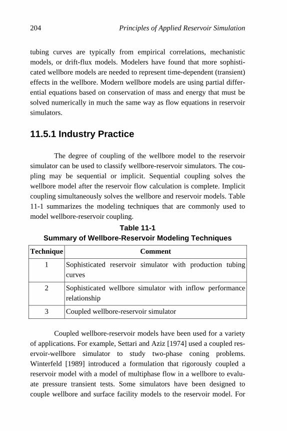
204 Principles of Applied Reservoir Simulation
tubing curves are typically from empirical correlations, mechanistic models, or drift-flux models. Modelers have found that more sophisti-cated wellbore models are needed to represent time-dependent (transient) effects in the wellbore. Modern wellbore models are using partial differ-ential equations based on conservation of mass and energy that must be solved numerically in much the same way as flow equations in reservoir simulators.
11.5.1 Industry Practice
The degree of coupling of the wellbore model to the reservoir simulator can be used to classify wellbore-reservoir simulators. The cou-pling may be sequential or implicit. Sequential coupling solves the wellbore model after the reservoir flow calculation is complete. Implicit coupling simultaneously solves the wellbore and reservoir models. Table 11-1 summarizes the modeling techniques that are commonly used to model wellbore-reservoir coupling.
Table 11-1 Summary of Wellbore-Reservoir Modeling Techniques
Technique Comment
1 Sophisticated reservoir simulator with production tubing curves
2 Sophisticated wellbore simulator with inflow performance relationship
3 Coupled wellbore-reservoir simulator
Coupled wellbore-reservoir models have been used for a variety
of applications. For example, Settari and Aziz [1974] used a coupled res-ervoir-wellbore simulator to study two-phase coning problems. Winterfeld [1989] introduced a formulation that rigorously coupled a reservoir model with a model of multiphase flow in a wellbore to evalu-ate pressure transient tests. Some simulators have been designed to couple wellbore and surface facility models to the reservoir model. For

Overview of the Modeling Process 205
example, Litvak and Darlow [1995] coupled a wellbore model to a com-positional simulator that was later used to study the performance of Prudhoe Bay.
11.6 Reservoir-Aquifer Model
A reservoir-aquifer system can be modeled in flow models using two different techniques: as a numerical aquifer model, or as an analytic aquifer model. Each technique is discussed below.
11.6.1 Numerical Aquifer Model
A reservoir-aquifer system can be modeled using small grid-blocks to define the reservoir and increasingly larger gridblocks to define the aquifer. This approach has the advantage of providing a numerically uniform analysis of the reservoir-aquifer system. The numerical aquifer model represents aquifer influx by extending the finite difference grid covering the reservoir to include the aquifer (Figure 11-9). Rock and fluid properties for the aquifer gridblocks must be defined. This ap-proach has the disadvantage of requiring more computer storage and computing time because additional gridblocks are needed to model the aquifer. A more time- and cost-effective means of representing an aqui-fer is to represent aquifer influx with an analytic model.
Aquifer Reservoir
Figure 11-9. Flow Model Grid for Numerical Aquifer Model
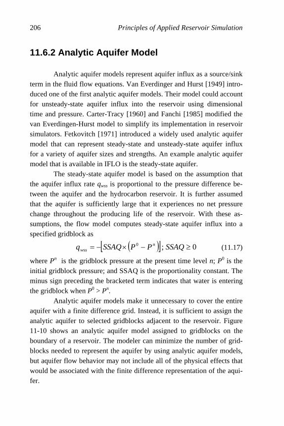
206 Principles of Applied Reservoir Simulation
11.6.2 Analytic Aquifer Model
Analytic aquifer models represent aquifer influx as a source/sink term in the fluid flow equations. Van Everdinger and Hurst [1949] intro-duced one of the first analytic aquifer models. Their model could account for unsteady-state aquifer influx into the reservoir using dimensional time and pressure. Carter-Tracy [1960] and Fanchi [1985] modified the van Everdingen-Hurst model to simplify its implementation in reservoir simulators. Fetkovitch [1971] introduced a widely used analytic aquifer model that can represent steady-state and unsteady-state aquifer influx for a variety of aquifer sizes and strengths. An example analytic aquifer model that is available in IFLO is the steady-state aquifer.
The steady-state aquifer model is based on the assumption that the aquifer influx rate qwss is proportional to the pressure difference be-tween the aquifer and the hydrocarbon reservoir. It is further assumed that the aquifer is sufficiently large that it experiences no net pressure change throughout the producing life of the reservoir. With these as-sumptions, the flow model computes steady-state aquifer influx into a specified gridblock as
( )[ ] 0;0 ≥−×−= SSAQPPSSAQq nwss (11.17)
where Pn is the gridblock pressure at the present time level n; P0 is the initial gridblock pressure; and SSAQ is the proportionality constant. The minus sign preceding the bracketed term indicates that water is entering the gridblock when P0 > Pn. Analytic aquifer models make it unnecessary to cover the entire aquifer with a finite difference grid. Instead, it is sufficient to assign the analytic aquifer to selected gridblocks adjacent to the reservoir. Figure 11-10 shows an analytic aquifer model assigned to gridblocks on the boundary of a reservoir. The modeler can minimize the number of grid-blocks needed to represent the aquifer by using analytic aquifer models, but aquifer flow behavior may not include all of the physical effects that would be associated with the finite difference representation of the aqui-fer.

Overview of the Modeling Process 207
AquiferReservoir
Figure 11-10. Flow Model Grid for Analytic Aquifer Model
Exercises
Exercise 11.1A Darcy’s Law in radial coordinates is
dr
dP
B
rhKQ
µπ
−=2
001127.0
where permeability K is in md, radius r is in ft, net thickness h is in ft, pressure P is in psia, viscosity µ is in cp, formation volume factor B is in reservoir volume per surface volume, and flow rate Q is in STB/day. Treat the derivative as a differential and solve for dP. Exercise 11.1B Integrate dP from pressure P at wellbore radius rw to pressure Pe at drainage radius re.
Exercise 11.1C Rearrange to find productivity index PI = Q / ∆P. Exercise 11.1D Estimate the PI for a well in a reservoir that has 10 ft. of net pay, permeability of 50 md, oil with viscosity of 1.5 cp and formation

208 Principles of Applied Reservoir Simulation
volume factor (FVF) of 1.4 RB/STB. Assume the wellbore radius is 0.3 ft. and the drainage radius is 500 ft. Exercise 11.1E What pressure drawdown is required to produce 100 STB/day of oil? Exercise 11.2 IFLO contains a few fieldwide controls. Data file EXAM4.DAT is a 2-D areal model of an undersaturated oil reservoir undergoing primary depletion. Modify data file EXAM4.DAT so that fieldwide pressure is not allowed to drop below the initial bubble point pressure using the run controls in Section 21.9. What effect does this have on the duration of the run? Exercise 11.3A What is the difference between laminar and inertial flow? Exercise 11.3B Does pipe roughness effect fluid flow in a circular pipe? Exercise 11.4 The Reynold’s number for flow in a circular pipe is 2500. Estimate the friction factor for turbulent flow assuming the pipe relative roughness is 0.01. Exercise 11.5 Kinematic viscosity η in centistokes is related to dynamic
viscosity µ in centipoises by the relationship ρµ=η where ρ is fluid
density in g/cm3. Suppose a fluid has density = 0.9 g/ cm3 and dynamic viscosity = 1.05 cp. What is its kinematic viscosity (in centistokes)? Exercise 11.6A Suppose water is flowing through a circular pipe with
volumetric flow rate q = 1000 barrels/day. The water density is ρ = 1 g/
cm3 = 1000 kg/m3 and the dynamic viscosity of water is µ = 1 cp = 0.001
Pa⋅s. The pipe length is 8000 ft and has a 5-inch inner diameter. The relative roughness of the pipe wall is 0.000144. What is the flow regime of the flowing water? Hint: calculate Reynolds number for flow.

Overview of the Modeling Process 209
Exercise 11.6B What is the friction factor?
Exercise 11.6C Plot pressure gradient dP/dL versus inclination angle θ.
Use 10° increments for the inclination angle in the range − 90° ≤ θ ≤ 90°. Express dP/dL in SI units and θ in degrees.
Exercise 11.6D What is the pressure gradient dP/dL at θ = 90°? Express your answer in psi/ft. Exercise 11.7 The pressure in a column of water is 1000 psia at a depth of 2300 ft. What is the pressure at a depth of 2200 ft. Assume the density of water is 1 g/cc, the acceleration of gravity is 9.8 m/s2. Express your answer in psia and kPa. Exercise 11.8A Data file EXAM8A.DAT is a 3-D model of a gas reser-voir undergoing primary depletion. Run EXAM8A.DAT and report the duration of the run. What are the average reservoir pressure, gas rate, water rate, aquifer influx rate and cumulative aquifer influx at the end of the run? Hint: look in ITEMP.TSS or ITEMP.ROF. Exercise 11.8B Data file EXAM8B.DAT is the same as file EXAM8A.DAT except that an analytic aquifer has been added. Run EXAM8B.DAT and report the duration of the run. What are the average reservoir pressure, gas rate, water rate, aquifer influx rate and cumulative aquifer influx at the end of the run? Explain the differences between Parts A and B.
210
Chapter 12
Conceptual Reservoir Scales
One of the most important goals of modeling is to reduce the risk associated with making decisions in an environment where knowledge is limited. The validity of data used in the decision-making process de-pends on the measurement technique used to obtain the data and the appropriate scale of applicability of the technique. Data validity provides information about risk. The integration of scale-dependent data into a cohesive reservoir description can reduce the risk of decision-making. This chapter introduces the concept of scale and discusses Giga Scale information.
12.1 Reservoir Sampling and Scales We can obtain a sense of just how well we understand the reser-voir by considering the fraction of reservoir area sampled by different techniques. As an example, suppose we want to find the size of the area sampled by a wellbore that has a 6-in. radius. If we assume the area is
circular, we can calculate the area as πr2 where r is the sampled radius.
The area sampled by a 6-in. radius wellbore is less than a square foot. To determine the fraction of area sampled, we normalize the sampled area with respect to the drainage area of a well. If we assume the drainage area of the well is a modest five acres, the drainage area is 218,000 sq. ft. What fraction of the drainage area is directly sampled by the wellbore?
Conceptual Reservoir Scales 211
The fraction of the area sampled by the well is three to four parts in a million. This is a tiny fraction of the area of interest.
A well log signal will expand the area that is being sampled. Suppose a well log can penetrate the formation up to five feet from the wellbore, which is a reasonably generous assumption. The fraction of area that has been sampled is now approximately four parts in ten thou-sand. The sample size in a drainage area of five acres is still a fraction of a percent. Core and well log data give a very limited view of the reservoir. A seismic section expands the fraction of area sampled, but the interpre-tation of seismic data is less precise. Seismic data is often viewed as “soft data” because of its dependence on interpretation. The reliability of seismic interpretation can be improved when correlated with “hard data” such as core and well log measurements. The range of applicability of measured data depends on the sam-pling technique. Did we take some core out of the ground, measure an electrical response from a well log, or detect acoustical energy? Figure 12-1 illustrates the ranges. Fayers and Hewett [1992] point out that scale definitions are not universally accepted, but do illustrate the relative scale associated with reservoir property measurements. Scale sizes range from the very big to the microscopic. Variations in the scale of data ap-plicability can be distinguished by defining conceptual scales. Figure 12-2 illustrates the system of reservoir scales that is adopted for use in the following discussion. The Giga Scale in Figure 12-2 includes information associated with geophysical techniques, such as reservoir architecture. Theories of regional characterization, such as plate tectonics, provide an intellectual framework within which Giga Scale measurement techniques, like seis-mic and satellite data, can be interpreted. The Mega Scale is the scale of reservoir characterization and includes well logging, pressure transient testing, and 3-D seismic analysis. The Macro Scale focuses on data sam-pling at the level of core analysis and fluid property analysis. The Micro Scale includes pore scale data obtained from techniques such as thin sec-tion analysis and measurements of grain-size distribution. Each of these scales contributes to the final reservoir flow model.
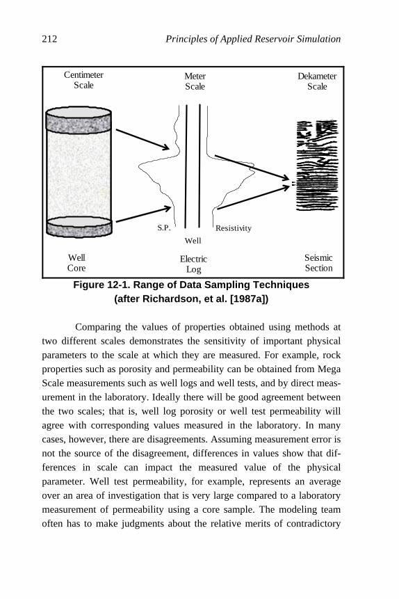
212 Principles of Applied Reservoir Simulation
CentimeterScale
MeterScale
DekameterScale
WellCore
ElectricLog
SeismicSection
S.P.
Well
Resistivity
Figure 12-1. Range of Data Sampling Techniques (after Richardson, et al. [1987a])
Comparing the values of properties obtained using methods at
two different scales demonstrates the sensitivity of important physical parameters to the scale at which they are measured. For example, rock properties such as porosity and permeability can be obtained from Mega Scale measurements such as well logs and well tests, and by direct meas-urement in the laboratory. Ideally there will be good agreement between the two scales; that is, well log porosity or well test permeability will agree with corresponding values measured in the laboratory. In many cases, however, there are disagreements. Assuming measurement error is not the source of the disagreement, differences in values show that dif-ferences in scale can impact the measured value of the physical parameter. Well test permeability, for example, represents an average over an area of investigation that is very large compared to a laboratory measurement of permeability using a core sample. The modeling team often has to make judgments about the relative merits of contradictory

Conceptual Reservoir Scales 213
data. The history matching process should recognize this source of un-certainty, as is discussed in subsequent chapters.
MacroScale
MegaScale
GigaScale
WellCore
ElectricLog
SeismicSection
S.P.Well
Resistivity
MicroScale
ThinSection
Figure 12-2. Reservoir Scales (after Haldorsen and Lake [1989] )
12.2 Reservoir Geophysics Seismic measurements discussed by authors such as Ausburn, et al. [1978], McQuillin, et al. [1984], Sheriff [1989], Dorn [1998], and Liner [2004] provide much of the Giga Scale data that can be directly used to characterize a reservoir. Historically, seismic analyses have been of interest primarily as a means of establishing the structural size of the reservoir. People did not believe that seismic data could resolve suffi-cient detail to provide information beyond overall reservoir structure. But that view has changed with the emergence of time-lapse seismic monitoring and reservoir geophysics [for example, see Richardson, 1989; Ruijtenberg, et al., 1990; Anderson, 1995; He, et al., 1996; Johnston, 1997; Fanchi, et al. 1999; de Waal and Calvert, 2003; Lumley, 2004].
Reservoir geophysics is the application of geophysical tech-niques to the production of subsurface resources during the producing life of a field. The resolution associated with reservoir geophysics tends to be more quantitative than the resolution associated with exploration

214 Principles of Applied Reservoir Simulation
geophysics. Exploration geophysics is the application of geophysical techniques to the search for commercial resources in the subsurface. By contrast, reservoir geophysics can use data from measurements in wells to calibrate the processing and interpretation of seismic measurements. The importance of reservoir geophysics to the reservoir management function makes it worthwhile to introduce some basic geophysical con-cepts.
Seismic waves are vibrations or disturbances that propagate from a source, such as an explosion or a shock wave, through the earth until they encounter a reflecting surface and are reflected into a detector, such as a geophone. Figure 12-3 shows a seismic trace. Each trace represents the signal received by a detector. Geophysical instruments measure the time it takes the seismic wave to propagate from the source to the reflec-tor and then to the receiver. This time is referred to as two-way travel time. It must be converted to depth for use in geological analysis.
Seismic Response
Sand
Shale
Model
100 ms
200 ms
5 1510 20 25
Figure 12-3. Seismic Trace for a Sand Wedge
(after Ruijtenberg [1990]; reprinted by permission of the Society of Petroleum Engineers)

Conceptual Reservoir Scales 215
One of the central problems in seismic data processing is deter-mining the time to depth conversion which may be considered the point where geology and geophysics meet [Medvin and Rennie, 1996]. When the time to depth conversion is applied to seismic data, it can change the relative depths of seismic amplitudes associated with adjacent traces and require a revision of the original interpretation.
The conversion of travel time data to formation depth requires that the velocity associated with each geologic zone be known or that it can be inferred as the wave evolves with time. Time to depth conversion calculations require models of seismic velocity in different types of ma-terials. Figure 12-4 illustrates the time to depth conversion process for a set of seismic traces in a 3-D volume element. The velocity model in the figure contains seismic velocities that can be used to map time values to depth values. Seismic velocities can be estimated from petrophysical models such as the IFLO petrophysical model described in Section 12.4. Petrophysical models use rock and fluid properties to estimate seismic velocities.
Velocity
Model
VelocityModel
Time (t)
Depth (z)
ty
x
y
x
z
Figure 12-4. Time to Depth Conversion Process
Changes to the direction of propagation of seismic waves occur at reflectors. A seismic reflection occurs at the interface between two regions with different acoustic impedances. Acoustic impedance is a fundamental seismic attribute. Acoustic impedance is defined as

216 Principles of Applied Reservoir Simulation
VZ ρ= (12.1)
where ρ is the bulk density of the medium and V is the compressional
velocity of the wave in the medium. Figure 12-5 illustrates a correlation between seismic wave velocity and the bulk density of different types of rock. Further discussion of rock properties and their relationship to seis-mic variables can be found in the literature [for example, Schön 1996; Mavko, et al., 1998; Tiab and Donaldson, 2003].
Shale
Sandstone
Salt
Anhydrite
Dolomite
Limestone
1.5 2.0 3 4 5 6 7 8 91.8
2.0
2.2
2.4
2.6
2.8
3.0
Velocity (km/sec) Figure 12-5. Seismic Wave Velocity and Bulk Density of Rock
(after Telford, et al. [1976]; reprinted by permission of Cambridge University Press; after Gardner, et al. [1974])
A change in acoustic impedance will cause a reflection of the sound wave. The ability to reflect a sound wave by a change in acoustic impedance is quantified in terms of the reflection coefficient. The reflec-tion coefficient R at the interface between two contiguous layers is defined in terms of acoustic impedances as
1122
1122
12
12
VV
VV
ZZ
ZZR
ρ+ρρ−ρ
=+−
= (12.2)
where subscripts 1 and 2 refer to the contiguous layers.
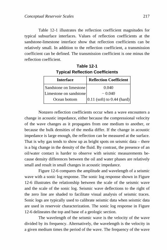
Conceptual Reservoir Scales 217
Table 12-1 illustrates the reflection coefficient magnitudes for typical subsurface interfaces. Values of reflection coefficients at the sandstone-limestone interface show that reflection coefficients can be relatively small. In addition to the reflection coefficient, a transmission coefficient can be defined. The transmission coefficient is one minus the reflection coefficient.
Table 12-1 Typical Reflection Coefficients
Interface Reflection Coefficient
Sandstone on limestoneLimestone on sandstone
Ocean bottom
0.040 − 0.040
0.11 (soft) to 0.44 (hard)
Nonzero reflection coefficients occur when a wave encounters a change in acoustic impedance, either because the compressional velocity of the wave changes as it propagates from one medium to another, or because the bulk densities of the media differ. If the change in acoustic impedance is large enough, the reflection can be measured at the surface. That is why gas tends to show up as bright spots on seismic data – there is a big change in the density of the fluid. By contrast, the presence of an oil/water contact is harder to observe with seismic measurements be-cause density differences between the oil and water phases are relatively small and result in small changes in acoustic impedance. Figure 12-6 compares the amplitude and wavelength of a seismic wave with a sonic log response. The sonic log response shown in Figure 12-6 illustrates the relationship between the scale of the seismic wave and the scale of the sonic log. Seismic wave deflections to the right of the zero line are shaded to facilitate visual analysis of seismic traces. Sonic logs are typically used to calibrate seismic data when seismic data are used in reservoir characterization. The sonic log response in Figure 12-6 delineates the top and base of a geologic section.
The wavelength of the seismic wave is the velocity of the wave divided by its frequency. Alternatively, the wavelength is the velocity in a given medium times the period of the wave. The frequency of the wave

218 Principles of Applied Reservoir Simulation
is a measure of the energy of the wave and is conserved as the wave propagates from one medium to another. The wavelength, however, can vary from one medium to another.
SeismicWave
SonicLog
Figure 12-6. Seismic Wave and Sonic Log Response
[after de Buyl, et al., 1988]
When waves overlap – or superpose – they create a wavelet, as shown in Figure 12-7. The time duration associated with the wavelet dis-
turbance is denoted ∆t. The wavelet has a velocity V in a medium, and
the period T=∆t is the width of the wavelet when plotted as a trace on a
time-map of seismic data. The length of the wave is equal to the velocity V times the period T. Thus, if the wavelet has a 10 millisecond period and the velocity is 5000 feet per second in a particular medium, then the length L of that wavelet is 50 feet.
If seismic data has enough resolving power to show the reflect-ing boundaries of a geologic layer, then the amplitudes of seismic waves may be useful for further characterizing the petrophysical properties of

Conceptual Reservoir Scales 219
the reservoir. For example, suppose a reservoir region is characterized by
porosity φ, permeability K, net thickness hnet, and oil saturation So. It may
be possible to correlate seismic amplitude with rock quality (for exam-
ple, Khnet or φkhnet) or oil productive capacity (for example, Soφkhnet).
When a correlation does exist between seismic amplitude and a grouping of petrophysical parameters, the correlation may be used to help guide the distribution of reservoir properties in areas between wells.
Wavelet
∆t V = velocity in mediumT = ∆t = period of wavelet
Figure 12-7. Seismic Wavelet
Figures 12-8a and 12-8b show two approaches to contouring a set of values at control points. The smooth contour lines shown in Figure 12-8a can be replaced by the irregular contour lines in Figure 12-8b if the irregular contour lines are supported by additional data. Seismic cor-relations can be used to justify the more heterogeneous contouring style shown in Figure 12-8b. A growing body of literature provides additional discussion of this application in the context of reservoir geophysics. For example, see de Buyl, et al. [1988], Evans [1996], Blackwelder, et al. [1996], Beasley [1996], Jack [1998], Waal and Calvert [2003], and Lum-ley [2004].

220 Principles of Applied Reservoir Simulation
Control Point
Figure 12-8a. Smooth Contour Lines
Figure 12-8b. Irregular Contour Lines
12.3 Correlating Reservoir Properties to Seismic Data
Reservoir geophysics has the potential to image important reser-voir parameters in regions between wells. The reservoir geophysical procedure requires the correlation of seismic data with reservoir proper-ties. Correlations are sought by making crossplots of seismic data with reservoir properties. The following are some correlation pairs:

Conceptual Reservoir Scales 221
Ü Seismic Amplitude versus Rock Quality
Ü Rock Quality equals a parameter group such as khnet or φkhnet,.
Ü Seismic Amplitude versus Oil Productive Capacity (OPC)
Ü OPC equals a parameter group such as Soφkhnet
Ü Acoustic Impedance versus Porosity If a statistically significant correlation is found, it can be used to guide the distribution of reservoir properties between wells. Ideally, the prop-erty distribution procedure will preserve reservoir properties at wells. De Buyl, et al. [1988] used reservoir geophysics to predict the reservoir properties of two wells. They correlated well log-derived prop-erties with seismically controlled properties. One such property is porosity. They then used the correlation to distribute properties. Maps drawn from seismically controlled distributions exhibited more hetero-geneity than conventional maps drawn from well log-derived properties. Heterogeneity based on seismically controlled distributions represents spatial variations in reservoir properties determined by direct observa-tion, albeit observation based on interpreted seismic data. Table 12-2 gives an indication of the technical success of the reservoir geophysical technique. Actual values of reservoir parameters at two well locations are compared with values predicted using both well log-derived properties and seismically controlled properties. This work by De Buyl, et al. [1988] is notable because it scientifically tests the seismic method: it makes predictions and then uses measurements to as-sess their validity. In this particular case, a reservoir characterization based on seismically controlled properties yielded more accurate predic-tions of reservoir properties than predictions made using a reservoir characterization based only on well data.
Although reservoir geophysical techniques are still evolving, it is possible to make some general statements about the relative value of this emerging technology. Table 12-3 summarizes the advantages and con-cerns associated with reservoir geophysics.

222 Principles of Applied Reservoir Simulation
Table 12-2 Predictions at New Wells from Seismic and Well Data
[de Buyl, et al., 1988]
Well Property Measured
Values Seismic Data
Predicted Well DataPredicted
I
Top of Reservoir (m) Gross Porosity (vol %)
Net φh (m)
-178.0 15.0 1.78
-175.015.51.53
-181.015.41.96
J
Top of Reservoir (m) Gross Porosity (vol %)
Net φh (m)
-182.0 13.9 1.08
-179.010.61.05
-174.08.0
0.15
Table 12-3 Reservoir Geophysics
Advantages Concerns
Ü Ability to “see” between wells
Ü Single realization en-hances Ü communication Ü understanding
Ü Cost of Ü data acquisition Ü analysis
Ü Time to build reservoir model Ü Limited applicability Ü Uncertainty of realization (unknown
without sensitivity analysis)
Data management and the integration of disciplines will play an
increasingly important role in the future of reservoir flow modeling [Thakur, 1996]. Many modelers have predicted that the integration of disciplines will manifest itself in reservoir flow modeling as finer 3-D models with more seismic and geological detail [He, et al., 1996; Ka-zemi, 1996; Uland, et al., 1997]. This prediction is being borne out with growing interest in shared earth models [Tippee, 1998; Fanchi, 2002a], model-centric working environments [Tobias, 1998], and reservoir flow

Conceptual Reservoir Scales 223
models with a million or more gridblocks [Dogru, 2000; Lasseter and Jackson, 2004].
12.4 IFLO Petrophysical Model
The petrophysical model in IFLO can be used to estimate both seismic attributes. Seismic attributes include compressional and shear velocities, and acoustic impedances. The IFLO petrophysical model is described here.
12.4.1 Compressional and Shear Velocities
Seismic compressional velocity and shear velocity are often cal-culated from the expressions [Mavko, et al., 1998]:
BP
KV
ρ
µ+
= 3
4sat
(12.3)
and
B
SVρµ
= (12.4)
where
VP = compressional velocity
VS = shear velocity
Ksat = saturated bulk modulus of porous medium
µ = shear modulus of porous medium
ρB = bulk density = (1-φ)ρm + φρf
The expressions for compressional velocity and shear velocity are gener-alized in the integrated flow model (IFM) to the functional form
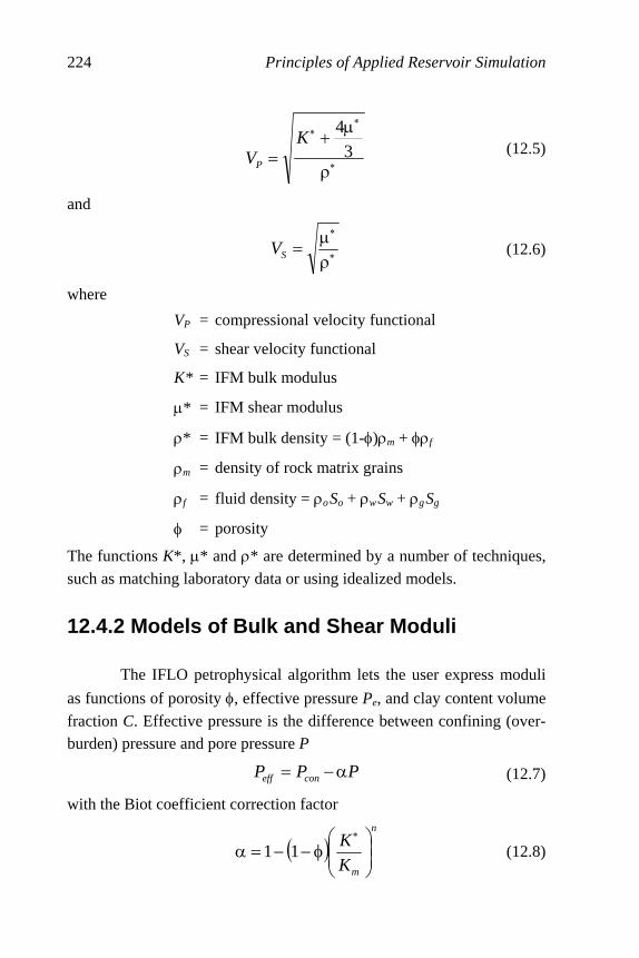
224 Principles of Applied Reservoir Simulation
∗
∗∗
ρ
µ+
= 34
KVP
(12.5)
and
∗
∗
ρµ
=SV (12.6)
where
VP = compressional velocity functional
VS = shear velocity functional
K* = IFM bulk modulus
µ* = IFM shear modulus
ρ* = IFM bulk density = (1-φ)ρm + φρf
ρm = density of rock matrix grains
ρf = fluid density = ρoSo + ρwSw + ρgSg
φ = porosity
The functions K*, µ* and ρ* are determined by a number of techniques, such as matching laboratory data or using idealized models.
12.4.2 Models of Bulk and Shear Moduli
The IFLO petrophysical algorithm lets the user express moduli
as functions of porosity φ, effective pressure Pe, and clay content volume
fraction C. Effective pressure is the difference between confining (over-burden) pressure and pore pressure P
PPP coneff α−= (12.7)
with the Biot coefficient correction factor
( )n
mK
K⎟⎟⎠
⎞⎜⎜⎝
⎛φ−−=α
∗
11 (12.8)
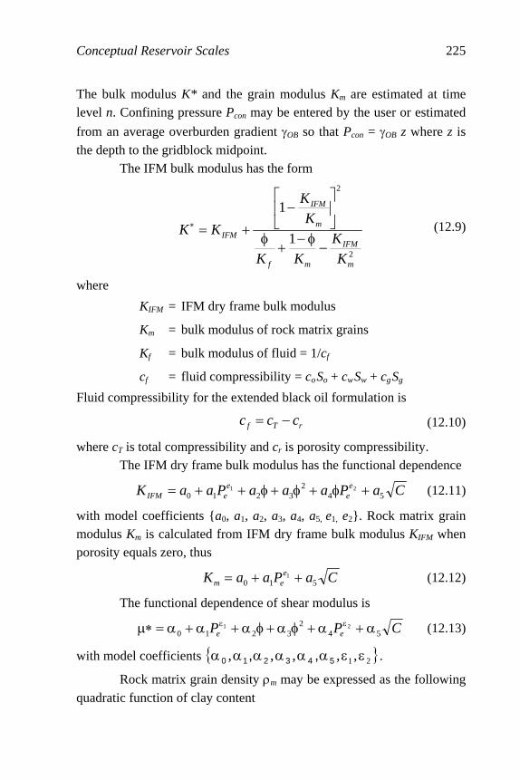
Conceptual Reservoir Scales 225
The bulk modulus K* and the grain modulus Km are estimated at time level n. Confining pressure Pcon may be entered by the user or estimated
from an average overburden gradient γOB so that Pcon = γOB z where z is the depth to the gridblock midpoint.
The IFM bulk modulus has the form
2
2
1
1
m
IFM
mf
m
IFM
IFM
K
K
KK
K
K
KK−
φ−+
φ
⎥⎦
⎤⎢⎣
⎡−
+=∗ (12.9)
where
KIFM = IFM dry frame bulk modulus
Km = bulk modulus of rock matrix grains
Kf = bulk modulus of fluid = 1/cf
cf = fluid compressibility = coSo + cwSw + cgSg
Fluid compressibility for the extended black oil formulation is
rTf ccc −= (12.10)
where cT is total compressibility and cr is porosity compressibility. The IFM dry frame bulk modulus has the functional dependence
CaPaaaPaaK ee
eeIFM 54
23210
21 +φ+φ+φ++= (12.11)
with model coefficients {a0, a1, a2, a3, a4, a5, e1, e2}. Rock matrix grain modulus Km is calculated from IFM dry frame bulk modulus KIFM when porosity equals zero, thus
CaPaaK eem 510
1 ++= (12.12)
The functional dependence of shear modulus is
CPP ee 542
321021 α+α+φα+φα+α+α=∗µ εε (12.13)
with model coefficients { }21,,,,, εεαααααα 543210 ,, .
Rock matrix grain density ρm may be expressed as the following quadratic function of clay content
226 Principles of Applied Reservoir Simulation
2210 CbCbbm ++=ρ (12.14)
with regression coefficients {b0, b1, b2}.
12.4.2.1 Constant Modu li (Gassmann) Model Bulk modulus is calculated from Gassmann’s [1951] equation as follows [Schön, 1996; McQuillin, et al., 1984]:
B
m
dry
mf
m
dry
drysat
K
K
KK
K
K
KKK
ρ=∗ρ
µ=∗µ
−φ−
+φ
⎥⎥⎦
⎤
⎢⎢⎣
⎡−
+==∗
,
,1
1
2
2
(12.15)
where
Ksat = saturated bulk modulus
Kdry = dry frame bulk modulus
Km = bulk modulus of rock matrix grains
Kf = bulk modulus of fluid = 1/cf
cf = fluid compressibility = coSo + cwSw + cgSg
µ = shear modulus
ρB = Bulk density = (1-φ)ρm + φρf
The user must enter Kdry, Km, φ, and ρm as arrays of constant values.
Grain modulus Km equals dry frame bulk modulus Kdry when porosity equals zero. Moduli in this model are not allowed to depend on effective pressure or clay content. Porosity and compressibility depend on pore pressure.

Conceptual Reservoir Scales 227
12.4.2.2 Han-Eberhart-Phillips Moduli
Table 12-4 presents regression model coefficients for the Han-Eberhart-Phillips (HEP) moduli [Fanchi, 2003a].
Table 12-4 Regression Model Coefficients for HEP Moduli*
Kdry Coefficient Regression Value µ* CoefficientRegression
Value
a0 5.2001 × 10⁶ α0 4.2958 × 10⁶
a1 2.9300 × 10⁴ α1 5.3952 × 10⁴
a2 −1.4307 × 10⁷ α2 −1.4952 × 10⁷
a3 6.9014 × 10⁶ α3 1.3948 × 10⁷
a4 5.7684 × 10² α4 −2.2544 × 10⁴
a5 −1.1936 × 10⁶ α5 −2.6009 × 10⁶
e1 1/3 ε1 1/3
e2 1/3 ε2 1/3
* For Kdry, µ* and Pe in psia; φ a fraction; and C a volume fraction. Cal-
culated moduli have units of psia.
12.4.3 Acoustic Impedance and Reflection Coefficients Acoustic impedance Z for compressional waves is defined as
PBVZ ρ= (12.16)
The reflection coefficient RC at the interface between two layers with acoustic impedances Z1 and Z2 is
228 Principles of Applied Reservoir Simulation
12
12
ZZ
ZZR
+−
= (12.17)
12.5 IFLO Application: Scheduling Time-Lapse Seismic Surveys
IFLO can be used to schedule time-lapse seismic surveys to op-
timize the acquisition of reservoir management information. Time-lapse seismology, also known as 4-D seismic, compares one 3-D seismic sur-vey with another 3-D seismic survey taken in the same geographic location but at a different time. Differences between the two 3-D seismic surveys arise from changes in reservoir properties such as pressure and saturation distributions. As an illustration of 4-D seismic monitoring, we consider the issue of scheduling two time-lapse seismic surveys with the goal of maximizing the acquisition of information that can be used in a reservoir management study.
The fluid properties in the first Society of Petroleum Engineers (SPE) comparative solution project [Odeh, 1981] are used with the res-ervoir characterization described in the second SPE comparative solution project [Weinstein, et al., 1986]. A cross section of an undersaturated oil reservoir with 15 layers is modeled. Permeability is isotropic and vertical permeability is assumed to be one tenth of horizontal permeability.
Layer 9 of the 15 layer cross section is the best oil target. The lowermost layer (layer 15) is a thick, water bearing aquifer layer. Gas is injected into the upper layers (layers 1 through 3) of the undersaturated oil reservoir cross section while oil is being produced from the lower layers (layers 9 through 12). All layers are in vertical communication. The per cent difference in acoustic response is relatively small in this example (less than 1% for the P-wave velocity to S-wave velocity ratio VP/VS), nevertheless the acoustic response for this example illustrates the following important features of time-lapse seismic monitoring.
The advance of the injected gas into the cross section is consid-ered at 180 days and 270 days. The gas front is highlighted by displaying
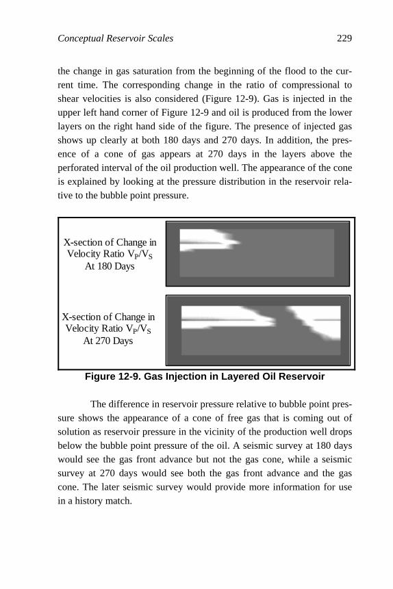
Conceptual Reservoir Scales 229
the change in gas saturation from the beginning of the flood to the cur-rent time. The corresponding change in the ratio of compressional to shear velocities is also considered (Figure 12-9). Gas is injected in the upper left hand corner of Figure 12-9 and oil is produced from the lower layers on the right hand side of the figure. The presence of injected gas shows up clearly at both 180 days and 270 days. In addition, the pres-ence of a cone of gas appears at 270 days in the layers above the perforated interval of the oil production well. The appearance of the cone is explained by looking at the pressure distribution in the reservoir rela-tive to the bubble point pressure.
X-section of Change inVelocity Ratio VP/VS
At 180 Days
X-section of Change inVelocity Ratio VP/VS
At 270 Days
Figure 12-9. Gas Injection in Layered Oil Reservoir
The difference in reservoir pressure relative to bubble point pres-sure shows the appearance of a cone of free gas that is coming out of solution as reservoir pressure in the vicinity of the production well drops below the bubble point pressure of the oil. A seismic survey at 180 days would see the gas front advance but not the gas cone, while a seismic survey at 270 days would see both the gas front advance and the gas cone. The later seismic survey would provide more information for use in a history match.
230 Principles of Applied Reservoir Simulation
Exercises Exercise 12.1A Run EXAM1.DAT and record the final time, final pres-sure and initial oil volume. Exercise 12.1B Multiply the volume of the reservoir in EXAM1.DAT by 0.5, 10 and 100. This can be done by altering the gridblock size (see Sec-tion 21.1). Make a table showing the final time, final pressure, and initial oil volume for each case. Exercise 12.1C How does the change in volume affect the pressure per-formance of the model as a function of time? Exercise 12.2 Repeat Exercise 12.1, but make the volume changes by modifying the grid dimensions using the pore volume modification op-tion in IFLO. Exercise 12.3 What is the seismic reflection coefficient R at the interface between two formations with equal acoustic impedances? Exercise 12.4A Effective bulk modulus K* can be written in terms of
porosity φ, dry rock bulk modulus KB, grain modulus KG and fluid
modulus KF as
[ ]G
B
GF
B K
Kb
K
b
K
bKK =
−φ−+
φ−
+=∗ ,1
1 2
Solve the above equation exactly for b and show your result. Hint: set
GB bKK = in K* and solve for b. The term KB should not appear in
your solution. Exercise 12.4B Using data from sonic log and laboratory measurements shown in the following table, calculate KB.

Conceptual Reservoir Scales 231
Parameter Value
VP (ft/s) 18,736
VS (ft/s) 10,036
VP / VS 1.87
µ* (psia) 3.61×10⁶
K* (psia) 7.30×10⁶
KG (psia) 9.70×10⁶
KB (psia)
KF (psia, brine) 2.97×10⁵
φ (fraction) 0.15
where
VP = Compressional velocity
VS = Shear velocity
K* = Effective bulk modulus
µ* = Shear modulus
Exercise 12.5A IFLO calculates P-wave and S-wave velocities using
*
*,
*
*3
4*
ρµ
=ρ
µ+= SP V
KV
where
VP = Compressional velocity
VS = Shear velocity
K* = IFM bulk modulus
µ* = IFM shear modulus
ρ* = IFM bulk density
The IFM bulk modulus has the form

232 Principles of Applied Reservoir Simulation
2
2
1
1
*
m
IFM
mF
m
IFM
IFM
K
K
KK
K
K
KK−
φ−+
φ
⎥⎦
⎤⎢⎣
⎡−
+=
where
VP = Compressional velocity
KIFM = IFM dry bulk modulus
Km = Bulk modulus of matrix grains
KF = Bulk modulus of fluid = 1/cF
cF = Fluid compressibility = coSo + cwSw + cgSg
Use the above information to estimate the minimum value that VP/VS can have. Exercise 12.5B Fill in the following table.
Parameter Value
VP / VS
µ* (psia) 3.61 × 10⁶
K* (psia) 7.30 × 10⁶
Km (psia) 9.70 × 10⁶
KF (psia, brine)2.97 × 10⁵
φ (fraction) 0.15
Exercise 12.6A Run XS-SPE2.DAT and record the time, pressure, oil rate and gas rate at the end of the run. Exercise 12.6B Use 3DView to create Figure 12-9.
233
Chapter 13
Flow Units
Giga Scale information helps define reservoir architecture, but is too coarse to provide the detail needed to characterize the reservoir enough to design a reservoir management plan. The Mega Scale is the scale at which we begin to integrate well log and pressure transient test data into a working model of the reservoir. This chapter introduces the role of well log and pressure transient test data in reservoir modeling. We then discuss the concept of flow unit.
13.1 Well Log Data Well logs provide valuable information about the formation within a few feet of the wellbore. A thorough discussion of well logging is beyond the scope of this book. We describe several concepts that are applicable to reservoir modeling. For more information, the interested reader should consult references such as Brock [1986], Bassiouni [1994], and Asquith and Krygowski [2004].
Well logs are obtained by running a tool into the wellbore. The tool can detect physical properties such as temperature, electrical current, radioactivity, or sonic reflections. Logging tools are designed to function best in certain types of environments. The environment depends on a variety of factors, including temperature, lithology, and fluid content. The theoretical analysis of log signals is usually based on the assumption

234 Principles of Applied Reservoir Simulation
that the formation is infinite in extent with homogeneous and isotropic properties. Tool performance will not be optimal in other environments.
Table 13-1 illustrates the type of information that can be ob-tained at the Mega Scale level from well log data. The most common interpretations of each log response are included in the table. For exam-ple, a high gamma ray response implies the presence of shales, while a low gamma ray response implies the presence of clean sands or carbon-ates.
The depth of investigation of a well log is a measure of the vol-ume of the formation that is primarily responsible for the well log signal. If we assume the formation has a uniform cylindrical shape for a forma-
tion with thickness h, then the volume investigated is φr2h where the
radius r is the depth of investigation into the formation, and φ is porosity.
Depth of investigation can range from a few inches to several feet.
Table 13-1 Well Log Response
Log Variable Response
Gamma ray Rock type
Ü Detects shale from in situ radioactivity.
Ü High gamma ray ⇒ shales
Ü Low gamma ray ⇒ clean sands or car-
bonates
Resistivity Fluid type
Ü Measures resistivity of formation water.
Ü High resistivity ⇒ hydrocarbons
Ü Low resistivity ⇒ brine
Density Porosity
Ü Measures electron density by detecting Compton scattered gamma rays. Elec-tron density is related to formation density. Good for detecting hydrocar-bon (HC) gas with low density compared to rock or liquid.
Ü Small response ⇒ low HC gas content
Ü Large response ⇒ high HC gas content

Flow Units 235
Acoustic (sonic)
Porosity
Ü Measures speed of sound in medium. Speed of sound is faster in rock than in fluid.
Ü Long travel time ⇒ slow speed ⇒ large pore space
Ü Short travel time ⇒ high speed ⇒ small
pore space
Neutron Hydrogen content
Ü Collisions slow fast neutrons to thermal energies. Thermal neutrons are captured by nuclei, which then emit detectable gamma rays. Note: Hydrogen has a large capture cross section for thermal neutrons. Good for detecting gas.
Ü Large response ⇒ high hydrogen content
Ü Small response ⇒ low hydrogen content
Spontaneous potential (SP)
Permeable beds
Ü Measures electrical potential (voltage) associated with movement of ions.
Ü Small response ⇒ impermeable shales
Ü Large response ⇒ permeable beds
Porosity and saturation can be obtained from well logs. For ex-
ample, the porosity of a logged interval from the formation density log is given by
fma
bma
ρ−ρρ−ρ
=φ (13.1)
where φ is porosity, and ρma, ρb and ρf are rock matrix density, bulk den-
sity and fluid density, respectively. Bulk density ρB of the medium is
( ) fmab φρ+ρφ−=ρ 1 (13.2)
The wetting phase saturation in a formation can be estimated from a re-sistivity log as
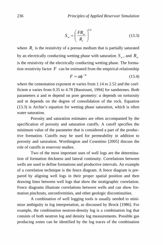
236 Principles of Applied Reservoir Simulation
n
t
ww R
FRS
1
⎟⎟⎠
⎞⎜⎜⎝
⎛= (13.3)
where tR is the resistivity of a porous medium that is partially saturated
by an electrically conducting wetting phase with saturation wS , and wR
is the resistivity of the electrically conducting wetting phase. The forma-
tion resistivity factor F can be estimated from the empirical relationship
maF −φ= (13.4)
where the cementation exponent m varies from 1.14 to 2.52 and the coef-ficient a varies from 0.35 to 4.78 [Bassiouni, 1994] for sandstones. Both parameters a and m depend on pore geometry: a depends on tortuosity and m depends on the degree of consolidation of the rock. Equation (13.3) is Archie’s equation for wetting phase saturation, which is often water saturation.
Porosity and saturation estimates are often accompanied by the specification of porosity and saturation cutoffs. A cutoff specifies the minimum value of the parameter that is considered a part of the produc-tive formation. Cutoffs may be used for permeability in addition to porosity and saturation. Worthington and Cosentino [2005] discuss the role of cutoffs in reservoir studies.
Two of the most important uses of well logs are the determina-tion of formation thickness and lateral continuity. Correlations between wells are used to define formations and productive intervals. An example of a correlation technique is the fence diagram. A fence diagram is pre-pared by aligning well logs in their proper spatial position and then drawing lines between well logs that show the stratigraphic correlation. Fence diagrams illustrate correlations between wells and can show for-mation pinchouts, unconformities, and other geologic discontinuities.
A combination of well logging tools is usually needed to mini-mize ambiguity in log interpretation, as discussed by Brock [1986]. For example, the combination neutron-density log is a combination log that consists of both neutron log and density log measurements. Possible gas producing zones can be identified by the log traces of the combination

Flow Units 237
neutron-density log. The presence of gas increases the density log poros-ity and decreases the neutron log porosity [Bassiouni, 1994, pg. 329]. If a sonic log is added to the log suite, quantitative information about lithol-ogy can be estimated using crossplots, and the log suite can be used to calibrate seismic data. Sonic log interpretation depends on lithology. In particular, the interval transit time in carbonates depends on the relative amount of pri-mary and secondary porosity. Primary porosity is associated with the matrix, and secondary porosity is associated with features such as frac-tures and vugs. Subtracting sonic porosity from total porosity recorded using neutron or density logs gives an estimate of secondary porosity. One more log, the gamma ray log, is usually added to the suite of logs used to evaluate gas bearing formations. The gamma ray log measures natural radioactivity in a formation. It provides a measurement of shale content, and can be used for identifying lithologies, correlating zones and correcting porosity log results in formations containing shale.
13.2 Pressure Transient Test Data
Pressure transient testing uses pressure changes measured at a well that are induced by changes in the flow rate of one or more wells. The variation in pressure is recorded as a function of time using pressure gauges. The information from pressure transient tests can be combined with data from other sources to obtain additional reservoir parameters. Analysis of the pressure response provides information that can be used to infer reservoir parameters such as flow capacity, average reservoir pressure in the drainage area, reservoir size, boundary and fault loca-tions, wellbore damage and stimulation, and well deliverability. We describe several concepts in this section that are applicable to reservoir modeling. Additional information about pressure transient testing can be found in such references as Matthews and Russell [1967], Earlougher [1977], Sabet [1991], Horne [1995], Chaudhry [2003a, b], and Brown and Hawkes [2005].
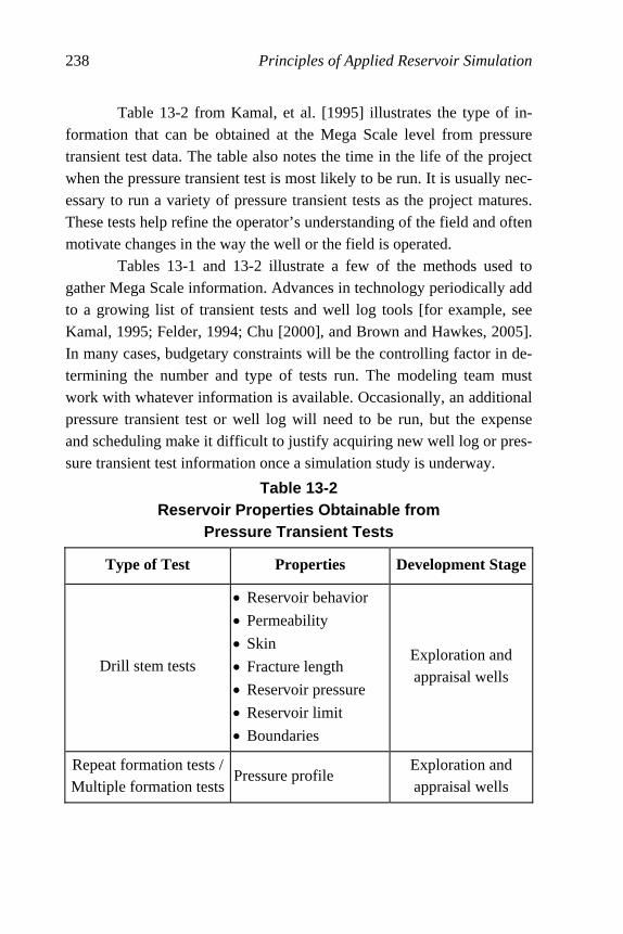
238 Principles of Applied Reservoir Simulation
Table 13-2 from Kamal, et al. [1995] illustrates the type of in-formation that can be obtained at the Mega Scale level from pressure transient test data. The table also notes the time in the life of the project when the pressure transient test is most likely to be run. It is usually nec-essary to run a variety of pressure transient tests as the project matures. These tests help refine the operator’s understanding of the field and often motivate changes in the way the well or the field is operated. Tables 13-1 and 13-2 illustrate a few of the methods used to gather Mega Scale information. Advances in technology periodically add to a growing list of transient tests and well log tools [for example, see Kamal, 1995; Felder, 1994; Chu [2000], and Brown and Hawkes, 2005]. In many cases, budgetary constraints will be the controlling factor in de-termining the number and type of tests run. The modeling team must work with whatever information is available. Occasionally, an additional pressure transient test or well log will need to be run, but the expense and scheduling make it difficult to justify acquiring new well log or pres-sure transient test information once a simulation study is underway.
Table 13-2 Reservoir Properties Obtainable from
Pressure Transient Tests
Type of Test Properties Development Stage
Drill stem tests
• Reservoir behavior
• Permeability
• Skin
• Fracture length
• Reservoir pressure
• Reservoir limit
• Boundaries
Exploration and appraisal wells
Repeat formation tests / Multiple formation tests
Pressure profile Exploration and appraisal wells

Flow Units 239
Drawdown tests
• Reservoir behavior
• Permeability
• Skin
• Fracture length
• Reservoir limit
• Boundaries
Primary, secondary and
enhanced recovery
Buildup tests
• Reservoir behavior
• Permeability
• Skin
• Fracture length
• Reservoir pressure
• Reservoir limit
• Boundaries
Primary, secondary,
and enhanced recovery
Falloff tests
• Mobility in various banks
• Skin
• Reservoir pressure
• Fracture length
• Location of front
• Boundaries
Secondary and enhanced recovery
Interference and pulse tests
• Communication between wells
• Reservoir type behavior
• Porosity
• Interwell permeability
• Vertical permeability
Primary, secondary, and enhanced
recovery

240 Principles of Applied Reservoir Simulation
Layered reservoir tests
• Properties of individ-ual layers
• Horizontal perme-ability
• Vertical permeability
• Skin
• Average layer pres-sure
• Outer boundaries
Throughout reservoir life
Step-rate tests
• Formation parting-pressure
• Permeability
• Skin
Secondary and enhanced recovery
In addition to providing information about individual well per-formance, wellbore damage, reservoir pressure, and reservoir fluid flow capacity, pressure transient testing can also provide information that can be used to estimate the distance to reservoir boundaries, structural dis-continuities, and communication between wells. For example, the radius of investigation for a pressure transient test in an oil well is the distance the pressure transient moves away from the oil well in the time interval following the change in flow rate. Assuming single-phase, radial flow, the radius of investigation may be estimated from a pressure buildup test in an oil well using the equation
T
i c
Ktr
φµ= 029.0 (13.5)
where the variables and units are defined in Table 13-3. For comparison, the radius of investigation for a pressure transient test in a gas well is an estimate of the distance the pressure transient moves away from the gas well in a specified time. It may be estimated from a pressure buildup test in a gas well using
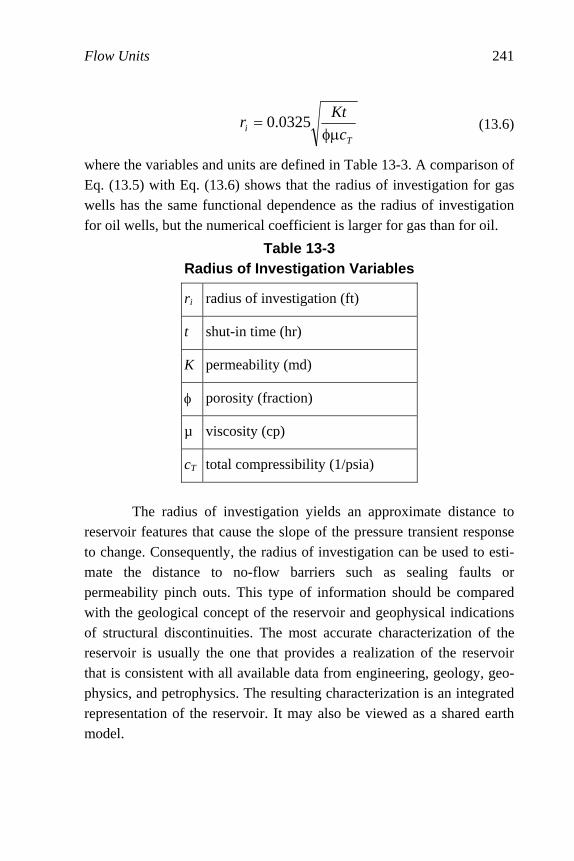
Flow Units 241
T
i c
Ktr
φµ= 0325.0 (13.6)
where the variables and units are defined in Table 13-3. A comparison of Eq. (13.5) with Eq. (13.6) shows that the radius of investigation for gas wells has the same functional dependence as the radius of investigation for oil wells, but the numerical coefficient is larger for gas than for oil.
Table 13-3 Radius of Investigation Variables
r i radius of investigation (ft)
t shut-in time (hr)
K permeability (md)
φ porosity (fraction)
µ viscosity (cp)
cT total compressibility (1/psia)
The radius of investigation yields an approximate distance to reservoir features that cause the slope of the pressure transient response to change. Consequently, the radius of investigation can be used to esti-mate the distance to no-flow barriers such as sealing faults or permeability pinch outs. This type of information should be compared with the geological concept of the reservoir and geophysical indications of structural discontinuities. The most accurate characterization of the reservoir is usually the one that provides a realization of the reservoir that is consistent with all available data from engineering, geology, geo-physics, and petrophysics. The resulting characterization is an integrated representation of the reservoir. It may also be viewed as a shared earth model.
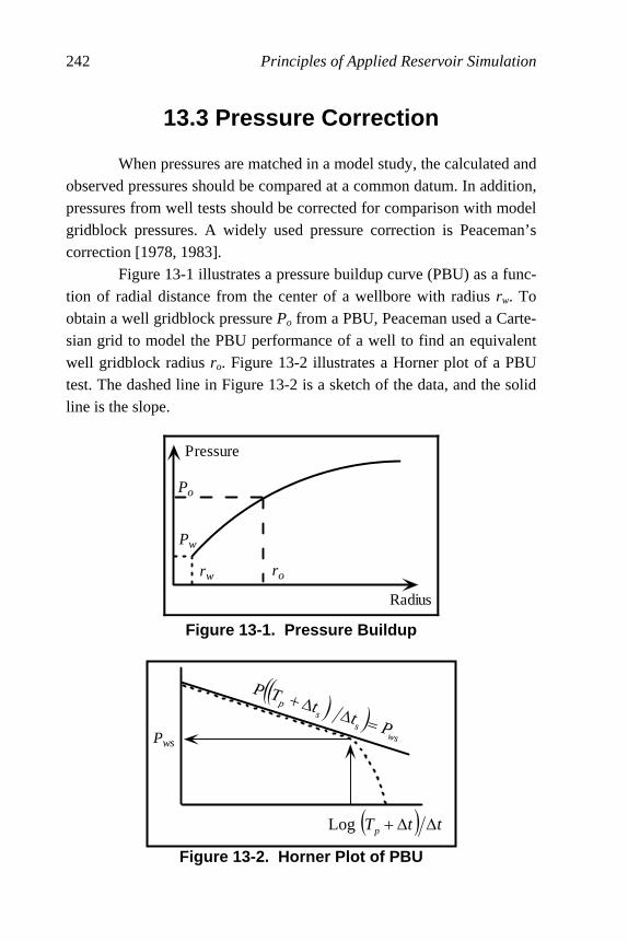
242 Principles of Applied Reservoir Simulation
13.3 Pressure Correction
When pressures are matched in a model study, the calculated and observed pressures should be compared at a common datum. In addition, pressures from well tests should be corrected for comparison with model gridblock pressures. A widely used pressure correction is Peaceman’s correction [1978, 1983]. Figure 13-1 illustrates a pressure buildup curve (PBU) as a func-tion of radial distance from the center of a wellbore with radius rw. To obtain a well gridblock pressure Po from a PBU, Peaceman used a Carte-sian grid to model the PBU performance of a well to find an equivalent well gridblock radius ro. Figure 13-2 illustrates a Horner plot of a PBU test. The dashed line in Figure 13-2 is a sketch of the data, and the solid line is the slope.
Pressure
Po
Radius
Pw
rw ro
Figure 13-1. Pressure Buildup
Figure 13-2. Horner Plot of PBU
Pws
( )(
)ws
ss
p
Ptt
TP
=∆∆+
( ) ttTp ∆∆+Log

Flow Units 243
Peaceman showed that the shut-in pressure Pws of an actual well
equals the simulator well gridblock pressure Po at a shut-in time ∆ts
given by
K
rct oTs
21688φµ=∆ (13.7)
where K is permeability, φ is porosity, µ is viscosity, and cT is total com-
pressibility. The relationship between gridblock pressure Po and flowing pressure Pwf at the wellbore is
⎥⎦
⎤⎢⎣
⎡+
µ−= S
r
r
Kh
QBPP
w
oowf ln2.141 (13.8)
where Q is the flow rate, B is formation volume factor, and S is skin. Shut-in time can be masked by wellbore storage effects. If it is, the shut-in pressure Pws may have to be obtained by extrapolating another part of the curve, such as the radial flow curve. Table 13-4 summarizes the pa-rameters involved in Peaceman’s correction for a consistent set of units. Odeh [1985] extended Peaceman’s work with 2-D models to 3-D mod-els.
Table 13-4 Oilfield Units for Peaceman’s Correction
Parameter Unit Parameter Unit
B RB/STB ro, rw ft
cT psia-1 S fraction
h ft ∆ts hr
K md ∆x, ∆y ft
Po, Pwf, Pws psia φ fraction
Q STB/day µ cp

244 Principles of Applied Reservoir Simulation
The equivalent well gridblock radius depends on the permeabil-ity isotropy of the reservoir. An isotropic reservoir in the horizontal plane is a reservoir in which x-direction permeability equals y-direction permeability (Kx = Ky). In this case, the equivalent well gridblock radius
is given in terms of the gridblock lengths {∆x, ∆y}, thus
( ) 21
2214.0 yxro ∆+∆= (13.9)
13.4 Integrating Scales: The Flow Unit All of the information collected at various scales must be inte-grated into a single, comprehensive, and consistent representation of the reservoir. The integration of data obtained at different scales is a difficult issue that is often referred to as the upscaling or scaleup problem [for example, see Oreskes, et al., 1994]. Attempts to relate data from two dif-ferent scales can be difficult. For example, permeability is often obtained from both pressure transient testing and routine core analysis. The re-spective permeabilities, however, may appear to be uncorrelated because they represent two different measurement scales. An important task of the scaleup problem is to develop a detailed understanding of how meas-ured parameters vary with scale. The focus on detail in one or more aspects of the reservoir flow modeling process can obscure the funda-mental reservoir concept in a model study. One way to integrate available data within the context of a “big picture” is to apply the flow unit concept. A flow unit is defined as “a volume of rock subdivided accord-ing to geological and petrophysical properties that influence the flow of fluids through it” [Ebanks, 1987]. Table 13-5 shows typical geologic and petrophysical properties. A classic application of the flow unit concept is presented in a paper by Slatt and Hopkins [1990].
A reservoir is modeled by subdividing its volume into an array of representative elementary volumes (REV). The REV concept is not the same as the flow unit concept. A flow unit is a contiguous part of the reservoir that has similar flow properties as characterized by geological

Flow Units 245
and petrophysical data. Several flow unit identification techniques are proposed in the literature, such as the modified Lorenz plot used by Gunter, et al. [1997].
Table 13-5 Properties Typically Needed to Define a Flow Unit
Geologic Petrophysical
Texture Mineralogy
Sedimentary Structure Bedding Contacts
Permeability Barriers
Porosity Permeability
Compressibility Fluid Saturations
A simplified variation of the modified Lorenz plot technique is to identify a flow unit by plotting normalized cumulative flow capacity as a function of depth. Normalized cumulative flow capacity Fm is calcu-lated as
nmhk
hkF
n
iii
m
iii
m ,,1;
1
1 K==
∑
∑
=
= (13.10)
where n is the total number of reservoir layers ik is the permeability of
layer i, and ih is the net thickness of layer i. The layers are numbered in
order from the shallowest layer i = 1 to the deepest layer i = m for a nor-malized cumulative flow capacity Fm at depth
∑=
+=m
iim hZZ
10 (13.11)
where Z0 is the depth to the top of layer 1 from a specified datum. A flow unit will appear on the plot as a line with constant slope. In Figure 13-3, a change in slope is interpreted as a change from one flow unit to an-other. Slope changes in Figure 13-3 occur at depths of 36 feet, 76 feet,

246 Principles of Applied Reservoir Simulation
92 feet, 108 feet, 116 feet, 124 feet, 140 feet, 152 feet, and 172 feet. The largest slope is between 108 feet and 116 feet, and corresponds to a high permeability zone. It is followed immediately by a low permeability zone at a depth of approximately 120 feet.
0.000
0.200
0.400
0.600
0.800
1.000
0 20 40 60 80 100 120 140 160 180 200
Depth (feet)
Nor
ma
lize
d C
um F
low
Cap
acity
Figure 13-3. Identifying flow units
Another plot that can be used to identify flow units is a plot of normalized cumulative flow capacity Fm versus a cumulative storage
capacity Φm defined by
nm
h
h
i
i
m ,,1,n
1=ii
m
1=ii
K=φ
φ=Φ
∑
∑ (13.12)
where n is the total number of reservoir layers and iφ is the porosity of
layer i. Again, the layers are numbered in order from the shallowest layer i = 1 to the deepest layer i = m. The analyst again looks for changes in
slope in the plot of Fm versus Φm.
Flow Units 247
Flow units usually contain one or more REVs. By contrast, the REV is the volume element that is large enough to provide statistically significant average values of parameters describing flow in the contained volume, but small enough to provide a meaningful numerical approxima-tion of the fundamental flow equations [for example, see Bear, 1972]. As noted by Fayers and Hewett [1992], “It is somewhat an act of faith that reservoirs can be described by relatively few REV types at each scale with stationary average properties.” Stolz and Graves [2003] have re-viewed different flow unit definition techniques and demonstrated that fluid flow in a layered system is sensitive to the defined flow unit. The flow unit concept is an effective means of managing the growing base of data being provided by geoscientists. Increasing refine-ment in geological models gives flow modelers more detail than they can use. Even today, with one hundred thousand to one million gridblock flow models, modelers cannot routinely use all of the information that is provided by computer-based geologic models. Computer-based geologic models often have in excess of one million grid points. It is still neces-sary to coarsen most detailed geologic models into representative flow units. A notable exception to this observation is the flow modeling work by Aramco modelers [Dogru, 2000; Dogru, et al., 2002]. They have shown that flow models that are created on the same scale as geoscience models can significantly reduce the number of runs needed to achieve a history match. An understanding of the big picture, even as a simple sketch, is a valuable resource for validating the ideas being quantified in a model. Richardson, et al. [1987b] sketched several common types of reservoir models: a deepwater fan; a sand-rich delta; a deltaic channel contrasted with a deltaic bar, and so forth. Their sketches illustrate what the reser-voir might look like for a specified set of assumptions. A sketch such as that in Figure 13-4 is a good tool for confirming that people from differ-ent disciplines share the same concept of a reservoir; it is a simple visual aid that enhances communication. In many cases, especially the case of relatively small fields, the best picture of the reservoir may only be a qualitative picture. When a more detailed study begins, the qualitative

248 Principles of Applied Reservoir Simulation
picture can be upgraded by quantifying parameters such as gross thick-ness in the context of the conceptual sketch of the reservoir.
Figure 13-4. Mississippi Delta
Confidence in model performance is acquired by using the
model to match historical field performance. History matching and model validation are discussed in greater detail in Chapter 18. From a technical perspective, flow models should be updated and refined as ad-ditional information is obtained from the field. In practice, the frequency of model updates depends on the importance of the resource being mod-eled to the enterprise.
13.5 IFLO Application: Valley Fill Waterflood
A valley fill reservoir is formed by the incision and fluvial ero-
sion of an existing facies. The valley is formed during a fall in relative
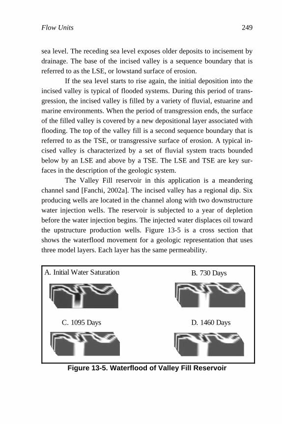
Flow Units 249
sea level. The receding sea level exposes older deposits to incisement by drainage. The base of the incised valley is a sequence boundary that is referred to as the LSE, or lowstand surface of erosion. If the sea level starts to rise again, the initial deposition into the incised valley is typical of flooded systems. During this period of trans-gression, the incised valley is filled by a variety of fluvial, estuarine and marine environments. When the period of transgression ends, the surface of the filled valley is covered by a new depositional layer associated with flooding. The top of the valley fill is a second sequence boundary that is referred to as the TSE, or transgressive surface of erosion. A typical in-cised valley is characterized by a set of fluvial system tracts bounded below by an LSE and above by a TSE. The LSE and TSE are key sur-faces in the description of the geologic system. The Valley Fill reservoir in this application is a meandering channel sand [Fanchi, 2002a]. The incised valley has a regional dip. Six producing wells are located in the channel along with two downstructure water injection wells. The reservoir is subjected to a year of depletion before the water injection begins. The injected water displaces oil toward the upstructure production wells. Figure 13-5 is a cross section that shows the waterflood movement for a geologic representation that uses three model layers. Each layer has the same permeability.
A. Initial Water Saturation B. 730 Days
C. 1095 Days D. 1460 Days
Figure 13-5. Waterflood of Valley Fill Reservoir

250 Principles of Applied Reservoir Simulation
Rather than using constant values of permeability for a layered system, a flow unit analysis can provide permeabilities for each layer. For example, suppose a flow unit analysis provides the layer permeabili-ties given in Table 13-6. The heterogeneous layer permeabilities shown in Table 13-6 have both a high permeability layer (layer 2) and a low permeability layer (layer 3). Rerunning the model shows that the perme-ability distribution in Table 13-6 results in earlier water production than the constant permeability case (see Exercise 13.5).
Table 13-6 Permeability for Valley Fill Model
Permeability (md) Layer
x-direction y-direction z-direction
1 100 100 10
2 300 300 30
3 50 50 5
Exercises Exercise 13.1A Use the data in the following table to make a porosity-permeability crossplot on semilogarithmic paper. Permeability should be plotted on the vertical, logarithmic axis and porosity should be plotted on the horizontal axis. Is the permeability distribution log-normal?
Flow Unit Exercise: Data from Table 5.35 of Wilhite [1986] for the Hiram No. 17 Well
Depth
Layer Top Bottom h Porosity
Permeabilityto air
(ft) (ft) (ft) (%) (md)
1 2880 2881 1.00 28.9 1271
2 2881 2882 1.00 28.5 1239
3 2882 2883 1.00 28.1 1184
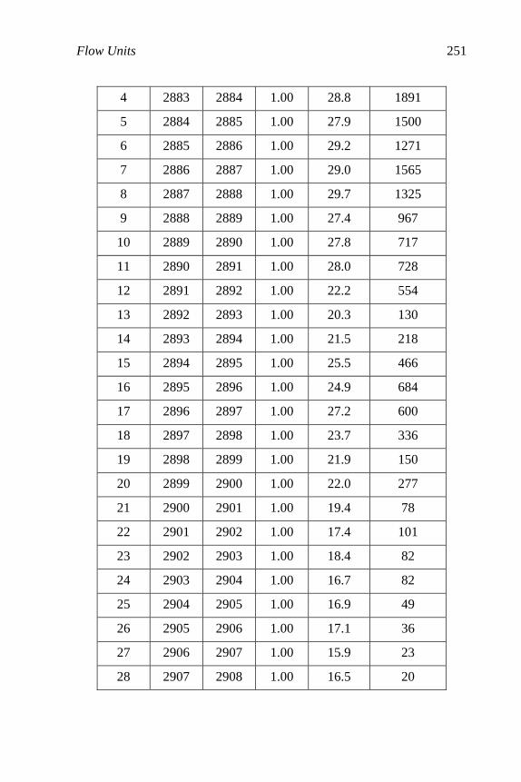
Flow Units 251
4 2883 2884 1.00 28.8 1891
5 2884 2885 1.00 27.9 1500
6 2885 2886 1.00 29.2 1271
7 2886 2887 1.00 29.0 1565
8 2887 2888 1.00 29.7 1325
9 2888 2889 1.00 27.4 967
10 2889 2890 1.00 27.8 717
11 2890 2891 1.00 28.0 728
12 2891 2892 1.00 22.2 554
13 2892 2893 1.00 20.3 130
14 2893 2894 1.00 21.5 218
15 2894 2895 1.00 25.5 466
16 2895 2896 1.00 24.9 684
17 2896 2897 1.00 27.2 600
18 2897 2898 1.00 23.7 336
19 2898 2899 1.00 21.9 150
20 2899 2900 1.00 22.0 277
21 2900 2901 1.00 19.4 78
22 2901 2902 1.00 17.4 101
23 2902 2903 1.00 18.4 82
24 2903 2904 1.00 16.7 82
25 2904 2905 1.00 16.9 49
26 2905 2906 1.00 17.1 36
27 2906 2907 1.00 15.9 23
28 2907 2908 1.00 16.5 20
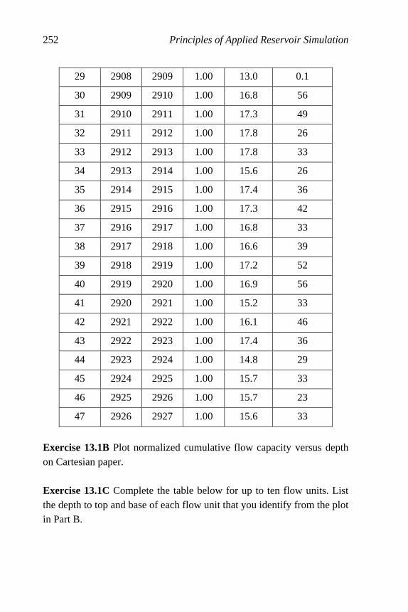
252 Principles of Applied Reservoir Simulation
29 2908 2909 1.00 13.0 0.1
30 2909 2910 1.00 16.8 56
31 2910 2911 1.00 17.3 49
32 2911 2912 1.00 17.8 26
33 2912 2913 1.00 17.8 33
34 2913 2914 1.00 15.6 26
35 2914 2915 1.00 17.4 36
36 2915 2916 1.00 17.3 42
37 2916 2917 1.00 16.8 33
38 2917 2918 1.00 16.6 39
39 2918 2919 1.00 17.2 52
40 2919 2920 1.00 16.9 56
41 2920 2921 1.00 15.2 33
42 2921 2922 1.00 16.1 46
43 2922 2923 1.00 17.4 36
44 2923 2924 1.00 14.8 29
45 2924 2925 1.00 15.7 33
46 2925 2926 1.00 15.7 23
47 2926 2927 1.00 15.6 33
Exercise 13.1B Plot normalized cumulative flow capacity versus depth on Cartesian paper. Exercise 13.1C Complete the table below for up to ten flow units. List the depth to top and base of each flow unit that you identify from the plot in Part B.
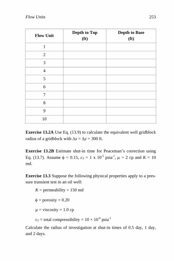
Flow Units 253
Flow Unit Depth to Top
(ft) Depth to Base
(ft)
1
2
3
4
5
6
7
8
9
10
Exercise 13.2A Use Eq. (13.9) to calculate the equivalent well gridblock
radius of a gridblock with ∆x = ∆y = 300 ft.
Exercise 13.2B Estimate shut-in time for Peaceman’s correction using
Eq. (13.7). Assume φ = 0.15, cT = 1 x 10⁻⁵ psia-1, µ = 2 cp and K = 10 md. Exercise 13.3 Suppose the following physical properties apply to a pres-sure transient test in an oil well:
K = permeability = 150 md
φ = porosity = 0.20
µ = viscosity = 1.0 cp
cT = total compressibility = 10 × 10-6 psia-1
Calculate the radius of investigation at shut-in times of 0.5 day, 1 day, and 2 days.
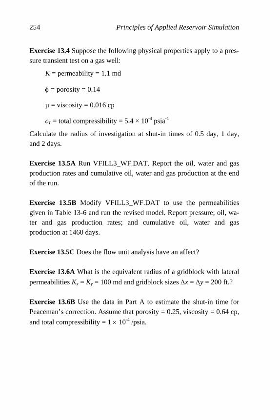
254 Principles of Applied Reservoir Simulation
Exercise 13.4 Suppose the following physical properties apply to a pres-sure transient test on a gas well:
K = permeability = 1.1 md
φ = porosity = 0.14
µ = viscosity = 0.016 cp
cT = total compressibility = 5.4 × 10⁻⁴ psia-1
Calculate the radius of investigation at shut-in times of 0.5 day, 1 day, and 2 days. Exercise 13.5A Run VFILL3_WF.DAT. Report the oil, water and gas production rates and cumulative oil, water and gas production at the end of the run. Exercise 13.5B Modify VFILL3_WF.DAT to use the permeabilities given in Table 13-6 and run the revised model. Report pressure; oil, wa-ter and gas production rates; and cumulative oil, water and gas production at 1460 days. Exercise 13.5C Does the flow unit analysis have an affect? Exercise 13.6A What is the equivalent radius of a gridblock with lateral
permeabilities Kx = Ky = 100 md and gridblock sizes ∆x = ∆y = 200 ft.? Exercise 13.6B Use the data in Part A to estimate the shut-in time for Peaceman’s correction. Assume that porosity = 0.25, viscosity = 0.64 cp,
and total compressibility = 1 × 10⁻⁴ /psia.

255
Chapter 14
Rock Properties Rock properties significantly influence the production of hydro-carbons from porous media. For example, oil production from unconsolidated sandstone reservoirs in the Gulf of Mexico depends on the relationship between permeability and fluid pressure. One way to approximate this effect in a flow model is to combine porosity-permeability models with porosity-fluid pressure relationships. This chapter describes the role of rock properties in reservoir flow modeling.
14.1 Porosity
One of the most fundamental properties of rock that a reservoir flow model must include is porosity, which is the fraction of a porous medium that is void space. The bulk volume VB of a porous medium is the sum of pore volume VP and grain volume VG, thus
GPB VVV += (14.1)
Porosity is the ratio of pore volume to bulk volume:
BP VV /=φ (14.2)
Dividing Eq. (14.1) by VB and using the definition of porosity expresses the grain volume in terms of porosity as
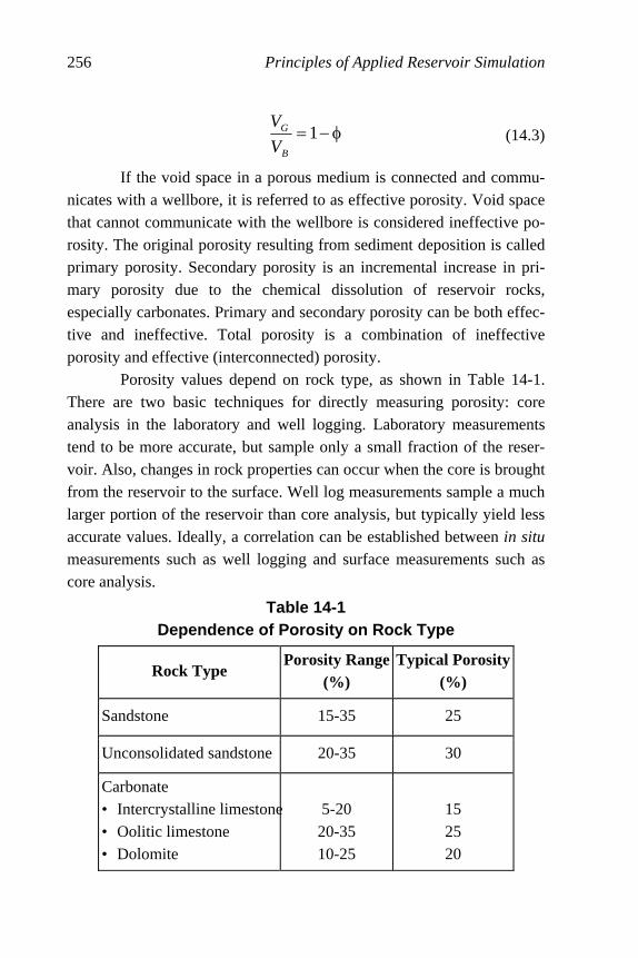
256 Principles of Applied Reservoir Simulation
φ−=1B
G
V
V (14.3)
If the void space in a porous medium is connected and commu-nicates with a wellbore, it is referred to as effective porosity. Void space that cannot communicate with the wellbore is considered ineffective po-rosity. The original porosity resulting from sediment deposition is called primary porosity. Secondary porosity is an incremental increase in pri-mary porosity due to the chemical dissolution of reservoir rocks, especially carbonates. Primary and secondary porosity can be both effec-tive and ineffective. Total porosity is a combination of ineffective porosity and effective (interconnected) porosity. Porosity values depend on rock type, as shown in Table 14-1. There are two basic techniques for directly measuring porosity: core analysis in the laboratory and well logging. Laboratory measurements tend to be more accurate, but sample only a small fraction of the reser-voir. Also, changes in rock properties can occur when the core is brought from the reservoir to the surface. Well log measurements sample a much larger portion of the reservoir than core analysis, but typically yield less accurate values. Ideally, a correlation can be established between in situ measurements such as well logging and surface measurements such as core analysis.
Table 14-1 Dependence of Porosity on Rock Type
Rock Type Porosity Range
(%) Typical Porosity
(%)
Sandstone 15-35 25
Unconsolidated sandstone 20-35 30
Carbonate • Intercrystalline limestone• Oolitic limestone • Dolomite
5-20 20-35 10-25
15 25 20

Rock Properties 257
Porosity compressibility is a measure of the change in porosity φ
as a function of fluid pressure P. It is defined as
dP
dc
φφ
=φ1
(14.4)
If 0φ is porosity at pressure 0P and φ is porosity at pressure P , the
integral of Eq. (14.4) yields the relationship
⎥⎥⎦
⎤
⎢⎢⎣
⎡φ=φ ∫ φ
P
P
dPc0
exp0 (14.5)
If porosity compressibility is constant with respect to pressure, the inte-gral in Eq. (14.5) can be evaluated and gives
[ ]Pc ∆φ=φ φexp0 (14.6)
where 〉P = P – P0. The first order approximation to Eq. (14.6) is
[ ] ( )[ ]000 11 PPcPc −+φ=∆+φ≈φ φφ (14.7)
Equation (14.7) is used in many reservoir flow simulators, including IFLO, to calculate the change in porosity with respect to changes in fluid pressure.
14.2 Permeability
The basic equation describing fluid flow in porous media is Darcy’s Law. Darcy's equation for linear, horizontal, single-phase flow is
x
PKAQ
∆∆
−=µ
001127.0 (14.8)
The physical variables are defined in oilfield units as
Q volume flow rate (bbl/day)
K permeability (md)
A cross-sectional area (ft2)

258 Principles of Applied Reservoir Simulation
〉P change in pressure (psi)
µ fluid viscosity (cp)
〉x length (ft)
Equation (14.8) shows that the movement of a single-phase fluid through a porous medium depends on cross-sectional area, pressure dif-ference 〉P, length 〉x of the flow path, and viscosity of the flowing fluid. The minus sign indicates that the direction of fluid flow is opposite to the direction of increasing pressure: the fluid flows from high pressure to low pressure in a horizontal (gravity-free) system. The proportionality constant in Eq. (14.8) is permeability.
Darcy’s Law correctly describes laminar flow, and may be used as an approximation of turbulent flow. Permeability calculated from Darcy’s Law is less than true rock permeability at turbulent flow rates. The linearity of Darcy’s Law is an approximation that is made by virtu-ally all commercial simulators. Fluid flow in a porous medium can have a nonlinear effect that is represented by the Forchheimer equation [Govier, 1978]. The nonlinear effect becomes more important in high flow rate environments such as some gas wells and in hydraulic fractur-ing [Barree and Conway, 2005].
Permeability is a measure of the connectivity of pore spaces. If we perform a dimensional analysis, we see that permeability has dimen-sions of L2 where L is a unit of length. The areal unit (L2) is physically related to the cross-sectional area of pore throats in rock.
A Micro Scale measurement of grain-size distribution shows that different grain sizes and shapes affect permeability. Permeability may be viewed as a mathematical convenience for describing the statistical be-havior of a given flow experiment. In this context, transient testing gives the best measure of permeability over a large volume. Despite their im-portance to the calculation of flow, permeability and its distribution will not be known accurately. Seismic data can help define the distribution of permeability between wells if a good correlation exists between seismic amplitude and a rock quality measurement that includes permeability.
Permeability depends on rock type. The two most common res-ervoir rock types are clastic reservoirs and carbonate reservoirs. The
Rock Properties 259
permeability in a clastic reservoir depends on pore size and is seldom controlled by secondary solution vugs. Compacted and cemented sand-stone rocks tend to have lower permeabilities than clean, unconsolidated sands. Productive sandstone reservoirs usually have permeabilities in the range of 10 md to 1000 md. The permeability in tight gas and coalbed methane reservoirs is less than 1 md.
Carbonate reservoirs are generally less homogeneous than clastic reservoirs and have a wider range of grain size distributions. The typical matrix permeability in a carbonate reservoir tends to be relatively low. Significant permeability in a carbonate reservoir may be associated with secondary porosity features such as vugs and oolites.
The presence of clay can adversely affect permeability. Clay ma-terial may swell on contact with fresh water, and the resulting swelling can reduce a rock's permeability by several orders of magnitude. In many cases vertical permeability is not measured and must be assumed. A rule of thumb is to assume that vertical permeability is ap-proximately one tenth of horizontal permeability. This is a reasonable assumption when there is no data to the contrary.
Natural or manmade fractures can significantly increase flow ca-pacity in both carbonate and clastic reservoirs. An extensive natural fracture system can provide high flow capacity conduits for channeling flow from the reservoir matrix to a wellbore. Naturally fractured reser-voirs are usually characterized by relatively high permeability, low porosity fractures and relatively low permeability, high porosity matrix. Most of the fluid is stored in the matrix, while flow from the reservoir to the wellbore is controlled by permeability in the fracture system.
14.2.1 Directional Permeability Permeability can be a complex function of spatial location and orientation. Spatial and directional variations of a function are described in terms of homogeneity, heterogeneity, isotropy, and anisotropy. If the value of a function does not depend on spatial location, it is called ho-mogeneous. The function is heterogeneous if its value changes from one

260 Principles of Applied Reservoir Simulation
spatial location to another. If the value of a function depends on direc-tional orientation, i.e. the value is larger in one direction than another, than the function is anisotropic. The function is isotropic if its value does not depend on directional orientation. Permeability is a function that can be both heterogeneous and anisotropic. To account for heterogeneity and anisotropy, the simple 1-D form of Darcy’s Law must be generalized. The discussion below closely follows the presentation in Chapter 4 of Fanchi [2000]. In general, flow occurs in dipping beds. To account for the effect
of gravity, we define a variable called the potential of phase as
( )zP ∆γ−=Φ (14.9)
where ∆z is depth from a datum, P is the pressure of phase and γ is
the pressure gradient associated with the gravity term. If we write Darcy’s Law for single phase flow in the form
dz
dKAq
Φµ
−=001127.0
(14.10)
we find that no vertical movement can occur when dΦ/dz = 0. Thus, Eq.
(14.10) expresses the movement of fluids in a form that accounts for gravity equilibrium. Darcy’s Law in one dimension says that rate is proportional to pressure gradient. This can be extended to three dimensions using vector notation. Darcy’s Law for single phase flow in three dimensions is
z
AKq
y
AKq
x
AKq
z
y
x
∂Φ∂
µ−=
∂Φ∂
µ−=
∂Φ∂
µ−=
001127.0
001127.0
001127.0
(14.11)
where the gradient of potential accounts for gravity effects. In vector notation we have
Rock Properties 261
Φ∇µ
−=A
Kq 001127.0
(14.12)
Equation (14.11) can be written in matrix notation as
⎥⎥⎥⎥⎥
⎦
⎤
⎢⎢⎢⎢⎢
⎣
⎡
∂Φ∂
∂Φ∂
∂Φ∂
µ−=
⎥⎥⎥⎥⎥
⎦
⎤
⎢⎢⎢⎢⎢
⎣
⎡
z
y
x
AK
q
q
q
z
y
x
001127.0 (14.13)
where permeability K and cross-sectional area A are treated as constants with respect to direction. A more general extension of Eq. (14.13) is
⎥⎥⎥⎥⎥
⎦
⎤
⎢⎢⎢⎢⎢
⎣
⎡
∂Φ∂
∂Φ∂
∂Φ∂
⎥⎥⎥⎥⎥
⎦
⎤
⎢⎢⎢⎢⎢
⎣
⎡
µ−=
⎥⎥⎥⎥⎥
⎦
⎤
⎢⎢⎢⎢⎢
⎣
⎡
z
y
x
KKK
KKK
KKK
A
q
q
q
zzzyzx
yzyyyx
xzxyxx
z
y
x
001127.0 (14.14)
where permeability is now treated either as a 3×3 matrix with nine ele-
ments or as a tensor of rank two [Fanchi, 2006]. The diagonal permeability elements {Kxx, Kyy, Kzz} represent the usual dependence of rate in one direction on pressure differences in the same direction. The off-diagonal permeability elements {Kxy, Kxz, Kyx, Kyz, Kzx, Kzy} account for the dependence of rate in one direction on pressure differences in orthogonal directions. Expanding Eq. (14.14) gives the corresponding set of equations that demonstrates this dependence:
⎥⎦
⎤⎢⎣
⎡∂Φ∂
+∂Φ∂
+∂Φ∂
µ−=
⎥⎦
⎤⎢⎣
⎡∂Φ∂
+∂Φ∂
+∂Φ∂
µ−=
⎥⎦
⎤⎢⎣
⎡∂Φ∂
+∂Φ∂
+∂Φ∂
µ−=
zK
yK
xK
Aq
zK
yK
xK
Aq
zK
yK
xK
Aq
zzzyzxz
yzyyyxy
xzxyxxx
001127.0
001127.0
001127.0
(14.15)

262 Principles of Applied Reservoir Simulation
In many practical situations it is mathematically possible to find
a coordinate system {x′, y′, z′} in which the permeability tensor has the
diagonal form
⎥⎥⎥
⎦
⎤
⎢⎢⎢
⎣
⎡
′′
′′
′′
zz
yy
xx
K
K
K
00
00
00
The coordinate axes {x′, y′, z′} are called the principal axes of the tensor and the diagonal form of the permeability tensor is obtained by a princi-pal axis transformation. The flow equations along the principal axes are
⎥⎦
⎤⎢⎣
⎡′∂Φ∂
µ−=
⎥⎦
⎤⎢⎣
⎡′∂Φ∂
µ−=
⎥⎦
⎤⎢⎣
⎡′∂Φ∂
µ−=
′′′
′′′
′′′
zK
Aq
yK
Aq
xK
Aq
zzz
yyy
xxx
001127.0
001127.0
001127.0
(14.16)
The principal axes in a field can vary from one point of the field to an-other because of permeability heterogeneity.
The form of the permeability tensor depends on the properties of the porous medium. The medium is said to be anisotropic if two or more elements of the diagonalized permeability tensor are different. The per-meability of the medium is isotropic if the elements of the diagonalized permeability tensor are equal, that is
KKKK zzyyxx === ′′′′′′ (14.17)
If the medium is isotropic, permeability does not depend on direction. If the isotropic permeability does not change from one position in the me-dium to another, the medium is said to be homogeneous in permeability. On the other hand, if the values of the elements of the permeability ten-sor vary from one point in the medium to another, both the permeability tensor and the medium are considered heterogeneous. Virtually all reser-voirs exhibit some degree of anisotropy and heterogeneity, but the flow

Rock Properties 263
behavior in many reservoirs can be approximated as homogeneous and isotropic. In Figure 14-1, Part A is a sketch of the drainage area of four production wells with isotropic permeability, and Part B is a sketch of the drainage area of four production wells with anisotropic permeability.
When a model is being designed, the modeling team should ac-count for the direction associated with permeability. In principle, simulators can take all of these effects into account. In practice, however, the tensor permeability discussed in the literature by, for example, Bear [1972], Lake [1988] or King and Mansfield [1999], is seldom included in a reservoir simulator. The usual assumption is that permeability is aligned along one of three orthogonal directions known as the principal axes of the tensor. This assumption has implications for model studies that should be considered when assessing model results (see Fanchi [1983]).
A. Isotropic (Kx = Ky) B. Anisotropic (Kx ≠ Ky)
Figure 14-1. Illustration of the Effect of Permeability Anisotropy on Drainage Area
14.3 Porosity-Permeability Models
Models relating permeability to porosity are often based on net-works of capillary tubes or the concept of hydraulic radius. This section reviews examples of porosity-permeability models from the literature and then generalizes them for use in a reservoir simulator.

264 Principles of Applied Reservoir Simulation
14.3.1 Capillary Tube Model
Flow of a fluid with viscosity µ through a capillary tube with ra-
dius r, porosity φ, cross-sectional area A and length L is given by
Poiseuille’s equation for viscous flow in a circular conduit. The perme-
ability capK of the capillary tube is
8
2rKcap φ= (14.18)
14.3.2 Hydraulic Radius Model
Hydraulic radius rh is the ratio of pore volume VP to pore surface area SP:
PB
PPh
SV
SVr
φ=
= (14.19)
where VB is the bulk volume of the sample [Guéguen and Palciauskas, 1994]. Defining specific surface area S as the pore surface area divided by the sample bulk volume,
BP VSS /= (14.20)
the hydraulic radius becomes
Srh φ= (14.21)
If we assume the permeability of the medium can be approximated as a capillary tube with radius rh, then we can use Eq. (14.18) to write
2
3
2
SB
rBK h
φ=
φ= (14.22)
where B is a constant that represents the model geometry. For a cylin-
drical tube that satisfies Poiseuille’s equation we have 81=B .

Rock Properties 265
14.3.3 Kozeny- Carman Model
The relationship between K and φ3 in Eq. (14.22) is an example of a Kozeny-Carman relation. If we assume the porous medium is a packing of spheres with diameter d, we have [Mavko, et al., 1998]
( )
dS
φ−=
1
2
3 (14.23)
and Eq. (14.22) becomes
( )223
1 φ−φ′=
dBK (14.24)
where the constant 3/2 is absorbed in the new proportionality constant
B′ . According to the percolation model, porosity below a percola-
tion porosity φc does not contribute to flow. The percolation effect is
taken into account by replacing φ with φ - φc in the Kozeny-Carman rela-
tion. The result is
( ) 23dBK cφ−φ′′= (14.25)
where B ′′ is a new proportionality constant. Equations (14.18), (14.24) and (14.25) suggest that permeability
and porosity are related by the proportionality
nK φ∝ (14.26)
where n has been observed to vary from n ≤ 2 to n ≥ 7. Equation (14.26) is a power law relationship between permeability and porosity that is suitable for use in a reservoir simulator. A more generalized algorithm relating porosity and permeability is presented below.
14.3.4 Porosity-Per meability Crossplots
The permeability models described above are idealized physical models. Measurements of porosity and permeability distributions in fields around the world have shown that porosity and permeability are
266 Principles of Applied Reservoir Simulation
correlated. The statistical distribution of porosity is often the normal (or Gaussian) distribution, and the statistical distribution of permeability is often log normal. Two empirical relationships between porosity and permeability have been observed and are widely used: the semilog cross-plot, and the log-log crossplot. The plot of porosity versus permeability is often referred to as a phi-k crossplot.
It is often necessary to use linear regression to quantify the straight line segments of a phi-k crossplot because there is a considerable amount of scatter in data plotted from real fields. The log-log model is obtained by fitting a regression line to a plot of the logarithm of porosity versus a logarithm of permeability. Permeability is related to porosity in the log-log model by
11
bK φα= (14.27)
with regression constants α1 and b1. If we specify a permeability K0 cor-
responding to a porosity φ0, Eq. (14.27) becomes
1
010bK φα= (14.28)
Dividing Eq. (14.27) by (14.28) shows that the log-log model satisfies
1
00
b
K
K⎟⎟⎠
⎞⎜⎜⎝
⎛
φφ
= (14.29)
Equation (14.29) is a power law relationship similar to Eq. (14.26). The
use of a reference permeability K0 and porosity φ0 lets us replace the pro-portionality in Eq. (14.26) with the equality in Eq. (14.29).
The semilog model is obtained by fitting a regression line to a plot of porosity versus the logarithm of permeability. In the semilog model, permeability is related to porosity by
( )φα= 22 expbK (14.30)
where α2 and b2 are constants determined by the regression analysis. If
we specify a permeability K0 corresponding to a porosity φ0, Eq. (14.30) becomes

Rock Properties 267
( )0220 exp φα= bK (14.31)
Dividing Eq. (14.30) by (14.31) shows that the semilog model satisfies
( )[ ]020
exp φ−φ= bK
K (14.32)
Equations (14.29) and (14.32) can be represented in a single al-gorithmic form as
( )[ ]0220
10
exp1
φ−φ+⎟⎟⎠
⎞⎜⎜⎝
⎛
φφ
= baaK
Kb
(14.33)
where K0 is the permeability corresponding to porosity φ0, and the coef-
ficients {a1, a 2, b1, b2} are determined empirically. Equation (14.33) is a generalized porosity-permeability relationship.
14.4 Permeability-Porosity-Fluid Pressure Relationships
The dependence of permeability on fluid pressure is specified
through the dependence of porosity on fluid pressure. Beginning with fundamental definitions, we obtain a relationship between porosity and fluid pressure that is similar to the result obtained by McKee, et al. [1988]. The porosity-fluid pressure relationship of interest here is
⎥⎥⎦
⎤
⎢⎢⎣
⎡⎟⎟⎠
⎞⎜⎜⎝
⎛
φ−−φ−
⎟⎟⎠
⎞⎜⎜⎝
⎛
φ−φ=φ
∫
∫
φ
φ
P
P
P
P
dPc
dPc
0
0
1exp11
1exp
0
0 (14.34)
If porosity compressibility and porosity change slowly with respect to fluid pressure, Eq. (14.34) may be written as
)]}(exp[1{1
)](exp[
00
00 PPc
PPc
−−φ−
−φ=φ
φ
φ(14.35)
268 Principles of Applied Reservoir Simulation
Equation (14.35) can be written to first order in the pressure change as
( )[ ] ( )[ ]0000
00
00
1exp
)]}(exp[1{1
)](exp[
PPcPPc
PPc
PPc
−+φ≈−φ≈
−−φ−
−φ=φ
φφ
φ
φ
(14.36)
Notice that Eq. (14.36) is in agreement with Eq. (14.7). By calculating changes in porosity as a function of changes in fluid pressure, we can use porosity-permeability relationships such as Eq. (14.33) to estimate the change in permeability as a result of a change in fluid pressure. Authors such as McKee, et al. [1988], Soares, et al. [2002], Reyes and Osisanya [2002], Raghavan and Chin [2004], and Schutjens, et al. [2004] provide additional discussion of the dependence of permeability on stress. Many porosity-permeability relationships have been published in the literature. For example, Nelson [2004] describes a catalog of porosity-permeability data sets for sandstones, and Jennings and Lucia [2003] present porosity-permeability relationships for carbonates.
14.5 IFLO Geomechanical Model
The geomechanical model in IFLO can be used to estimate ge-omechanical parameters. The calculation of geomechanical parameters makes it possible to include pressure-dependent changes to permeability in well and transmissibility calculations. This section describes the IFLO geomechanical model.
14.5.1 Poisson’s Ratio and Young’s Modulus
Poisson’s ratio ν is calculated as
22
225.0
SP
SP
VV
VV
−−
=ν (14.37)
where PV is compressional or P-wave velocity, and SV is shear or S-
wave velocity. Young’s modulus E is calculated from Poisson’s ratio as
Rock Properties 269
( )µν+= 12E (14.38)
where µ is shear modulus.
Dynamic measurements of Young’s modulus and Poisson’s ratio are approximations of the static values needed for geomechanical calcu-lations. To obtain static values for Young’s modulus and Poisson’s ratio, a conversion calculation must be made [Wang, 2000; Tiab and Donaldson, 2003]. The dynamic to static conversion algorithm for Young’s modulus E is
( )( )e
e
bds
Pbbb
Paaa
caEE
log
log
21
21
+=
+=
+=
(14.39)
where subscript s denotes static and subscript d denotes dynamic. The coefficients {a, a1, a2, b, b1, b2, c} are empirical fit parameters, and Pe is effective pressure. An analogous dynamic to static conversion algorithm may be specified for Poisson’s ratio.
14.5.2 Uniaxial Compaction, Horizontal Stress and Fracture Gradient
Uniaxial compaction ∆h is estimated using
Phch net∆φ⎟⎟⎠
⎞⎜⎜⎝
⎛ν−ν+
=∆ φ1
1
3
1 (14.40)
where hnet is net thickness, φ is porosity, cφ is porosity compressibility,
and the change in pore pressure is ∆P = P - Pinit. Pore pressure is set equal to the fluid pressure being used as a primary variable in the solu-tion of the fluid flow equations.
Total horizontal stress σH is estimated as
( ) PPPconH α+α−ν−
ν=σ
1 (14.41)
with the Biot coefficient correction factor
270 Principles of Applied Reservoir Simulation
( )n
mK
K⎟⎟⎠
⎞⎜⎜⎝
⎛φ−−=α
∗
11 (14.42)
Fracture gradient γF is estimated as [Tiab and Donaldson, 2003]
z
Pconf ν+
ν=γ
1 (14.43)
14.5.3 Permeability-Poro sity-Fluid Pressure Algorithm
The dependence of permeability on fluid pressure is made ex-plicit by substituting Eq. (14.36) into Eq. (14.33) to obtain
( )[ ] ( )[ ]0022010
exp1 1 PPcbaPPcaK
K b −φ+−+= φφ (14.44)
The coefficients {a1, a2, b1, b2} are determined empirically. Equation (14.44) is an algorithm that relates permeability, porosity and fluid pres-sure. The effect of pressure on permeability may be included in the calculation of well productivity index and transmissibility.
14.6 IFLO Application: Geomechanics and Compaction
Geomechanical properties give us insight into the behavior of
the structure of the reservoir and the impact of structural changes on fluid flow. The conventional approach to coupling geomechanics and fluid flow is to solve two sets of nonlinear equations representing fluid flow and geomechanical deformation [Settari, et al., 2001; Settari [2002]; Yale, 2002; Tran, et al., 2002; Dean, et al., 2003]. The solution tech-niques range from full coupling in which both sets of equations are solved simultaneously at each timestep to varying degrees of partial cou-pling.

Rock Properties 271
The relative merits of coupled versus uncoupled formulations have been discussed in the literature. Yale [2002] argues that tight cou-pling between geomechanical and fluid flow models can more accurately account for the effect of heterogeneity, anisotropy and inelastic deforma-tion on fluid flow if there is enough information to properly characterize the algorithms used in a tightly coupled fluid flow simulator. Dean, et al. [2003] evaluated the degree of coupling for four sample problems and concludes that the “coupling techniques produce similar results and one’s selection of a technique is determined by ease of implementation, program availability, numerical stability, and computational efficiency. No technique worked best on all four problems.”
An important practical problem with the routine inclusion of ge-omechanical calculations in reservoir management studies is that conventional geomechanical simulators require a substantial increase in computer processing time to perform both geomechanical calculations and fluid flow calculations. Furthermore, geomechanical algorithms re-quire input data that may not be available. Geomechanical calculations made by the integrated flow model IFLO minimize these issues because the IFLO geomechanical algorithm requires little incremental computer processing time and requires minimal additional input data [Fanchi, 2003a, 2003c]. To achieve these objectives, the IFLO compaction calcu-lation relies on simplifying physical assumptions. Conventional geomechanical models include the compacting reservoir deformation effects shown in the upper half of Figure 14-2, namely surface extension, compression, and reservoir compaction. The IFLO compaction model approximates all of these effects as uniaxial compaction of the reservoir, which is sketched in the lower half of Figure 14-2. The goal of this ap-plication is to discuss the validity of the IFLO compaction model approximation.
The traditional formulation of a flow simulator with a pressure dependent porosity does include the calculation of geomechanical effects associated with the effect of changing pressure on porosity. This calcula-tion depends on the rock compressibility term. The traditional formulation of a black oil simulator assumes that rock compressibility is satisfactorily represented by porosity compressibility. The IFM solution
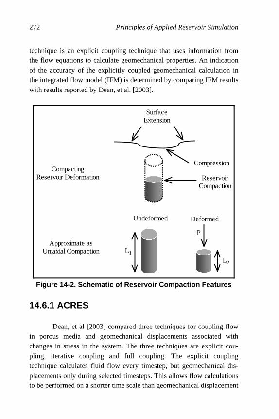
272 Principles of Applied Reservoir Simulation
technique is an explicit coupling technique that uses information from the flow equations to calculate geomechanical properties. An indication of the accuracy of the explicitly coupled geomechanical calculation in the integrated flow model (IFM) is determined by comparing IFM results with results reported by Dean, et al. [2003].
SurfaceExtension
Compression
ReservoirCompaction
Undeformed Deformed
CompactingReservoir Deformation
Approximate asUniaxial Compaction L1
L2
P
Figure 14-2. Schematic of Reservoir Compaction Features
14.6.1 ACRES
Dean, et al [2003] compared three techniques for coupling flow in porous media and geomechanical displacements associated with changes in stress in the system. The three techniques are explicit cou-pling, iterative coupling and full coupling. The explicit coupling technique calculates fluid flow every timestep, but geomechanical dis-placements only during selected timesteps. This allows flow calculations to be performed on a shorter time scale than geomechanical displacement
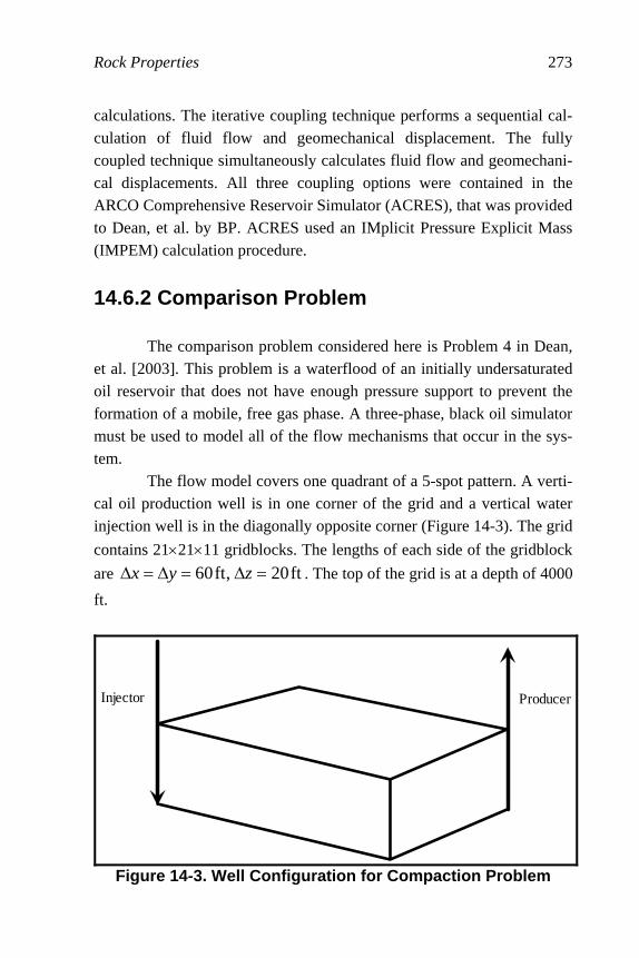
Rock Properties 273
calculations. The iterative coupling technique performs a sequential cal-culation of fluid flow and geomechanical displacement. The fully coupled technique simultaneously calculates fluid flow and geomechani-cal displacements. All three coupling options were contained in the ARCO Comprehensive Reservoir Simulator (ACRES), that was provided to Dean, et al. by BP. ACRES used an IMplicit Pressure Explicit Mass (IMPEM) calculation procedure.
14.6.2 Comparison Problem
The comparison problem considered here is Problem 4 in Dean, et al. [2003]. This problem is a waterflood of an initially undersaturated oil reservoir that does not have enough pressure support to prevent the formation of a mobile, free gas phase. A three-phase, black oil simulator must be used to model all of the flow mechanisms that occur in the sys-tem.
The flow model covers one quadrant of a 5-spot pattern. A verti-cal oil production well is in one corner of the grid and a vertical water injection well is in the diagonally opposite corner (Figure 14-3). The grid
contains 21×21×11 gridblocks. The lengths of each side of the gridblock
are ft20,ft60 =∆=∆=∆ zyx . The top of the grid is at a depth of 4000
ft.
ProducerInjector
Figure 14-3. Well Configuration for Compaction Problem

274 Principles of Applied Reservoir Simulation
Dean, et al. [2003] defined the following petrophysical parame-ters for this problem: Poisson’s ratio ν is 0.35, elastic (Young’s)
modulus E is 5×10⁴ psia, and grain density is 2.7 g/cc. Rock compressi-
bility is 4.15×10⁻⁵ / psia. Dry frame bulk modulus was calculated using
( ) ( ) µ−⎥⎦
⎤⎢⎣
⎡ν−ν+
ν−=
3
4
211
1EK (14.45)
where shear modulus µ was calculated as
( )ν+=µ12
E (14.46)
The dry frame bulk modulus for the IFLO petrophysical algorithm was
calculated to be 5.56×10⁴ psia, and the corresponding shear modulus is
1.85×10⁴ psia. Although the IFLO calculation can use fluid substitution,
conventional geomechanical flow simulators cannot, so grain modulus was set equal to dry frame bulk modulus in IFLO for this application.
14.6.3 Initial Conditions
Reservoir pressure is 3010 psi at a depth of 4010 ft. Reservoir porosity is 30%. Reservoir permeability varies by layer. Starting at the top layer, horizontal permeability for each layer is 5 md, 100 md, 20 md, 20 md, 20 md, 100 md, 20 md, 20 md, 100 md, 20 md and 20 md. Verti-cal permeabilities are 0.01 times horizontal permeabilities.
The reservoir is undersaturated with oil, water and gas satura-tions equal to 80%, 20% and 0% respectively. The bubble point pressure of the oil is 3000 psi. Details of fluid properties and rock-fluid interac-tion properties are presented in Dean, et al. [2003].
The water injection well in the model had a prescribed water in-jection rate of 500 STB/day and the production well in the Dean, et al. model had a prescribed liquid production rate of 750 STB/day. IFLO does not have a liquid production rate option, but it does have a fluid production rate option. Consequently, the IFLO model used a prescribed fluid production rate of 750 STB/day. The two production well options
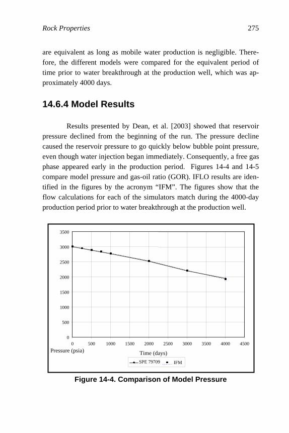
Rock Properties 275
are equivalent as long as mobile water production is negligible. There-fore, the different models were compared for the equivalent period of time prior to water breakthrough at the production well, which was ap-proximately 4000 days.
14.6.4 Model Results
Results presented by Dean, et al. [2003] showed that reservoir pressure declined from the beginning of the run. The pressure decline caused the reservoir pressure to go quickly below bubble point pressure, even though water injection began immediately. Consequently, a free gas phase appeared early in the production period. Figures 14-4 and 14-5 compare model pressure and gas-oil ratio (GOR). IFLO results are iden-tified in the figures by the acronym “IFM”. The figures show that the flow calculations for each of the simulators match during the 4000-day production period prior to water breakthrough at the production well.
Figure 14-4. Comparison of Model Pressure
0
500
1000
1500
2000
2500
3000
3500
0 500 1000 1500 2000 2500 3000 3500 4000 4500
Time (days)Pressure (psia)
IFMSPE 79709

276 Principles of Applied Reservoir Simulation
Figure 14-5. Comparison of Model GOR
Figure 14-6 compares model calculated compaction for the pro-duction well column [private communication from R.H. Dean, 7 March 2004]. The IFLO compaction in the production well column is approxi-mately 80% of the compaction calculated by ACRES after 4000 days of production. The average compaction of each layer of gridblocks in IFLO is calculated as the average compaction of all gridblocks in the layer. The sum of these layer average compaction values gives the average compac-tion calculated by IFLO. Figure 14-7 compares the average compaction of IFLO to the uniaxial compaction calculated using Eq. (14.40), the set of constant petrophysical parameters defined by Dean, et al. [2003], and pore volume weighted average reservoir pressure from IFLO. IFLO compaction results are comparable to results that would be calculated using a uniaxial compaction approximation.
0
200
400
600
800
1000
1200
1400
1600
0 500 1000 1500 2000 2500 3000 3500 4000 4500
Time (days)GOR (scf/stb)
SPE 79709 IFM

Rock Properties 277
Figure 14-6. Comparison of Compaction of the Production
Well Column
Figure 14-7. Uniaxial Compaction
0.0
0.5
1.0
1.5
2.0
2.5
3.0
3.5
4.0
0 500 1000 1500 2000 2500 3000 3500 4000 4500
Time (days)Subsidence (ft)SPE 79709 - Well IFM - Well
0.0
0.5
1.0
1.5
2.0
2.5
0 500 1000 1500 2000 2500 3000 3500 4000 4500
Time (days)Subsidence (ft)Uniaxial - Avg P IFM - Sum Compacted Cells

278 Principles of Applied Reservoir Simulation
Exercises
Exercise 14.1 Derive Eq. (14.5). Exercise 14.2 A sandstone core sample is cleanly cut and carefully measured in a laboratory. The cylindrical core has a length of 3 inches and a diameter of 0.75 inch. The core is dried and weighed. The dried core weighs 125.00 grams. The core is then saturated with fresh water. The water saturated core weighs 127.95 grams. Determine the porosity of the sandstone core. Neglect the weight of air in the dried core and as-sume the density of water is 1 g/cc. Exercise 14.3A Consider a cylindrical core plug that has a radius of 0.5 in. and a length of 2 in. Suppose the core is flooded with an oil that has viscosity = 0.5 cp, formation volume factor = 1.0 RB/STB, and a meas-ured flow rate = 0.1 BOPD (barrel of oil per day). If the pressure drop from the inlet to the outlet is 20 psia, what is the permeability of the plug? Hint: Express area A in sq. ft. and length L in ft. Solve Darcy’s Law for permeability. Recall that Darcy’s Law is
B L
P A k 0.001127 = Q
µ∆
where permeability k is in md, area A is in sq. ft., pressure P is in psia, length L is in ft, viscosity µ is in cp, formation volume factor B is in res-ervoir volume per surface volume, and flow rate Q is in BOPD. Exercise 14.3B Suppose that water (viscosity = 1.0 cp, FVF = 1.0 RB/STB) was used instead of oil in Part A. Use the permeability calcu-lated in Part A to estimate the water flow rate. We are assuming that the permeability to single phase flow of water is the same as the permeabil-ity to single phase flow of oil. Exercise 14.4 The pressure at an injection well is 3000 psia and the pres-sure at a production well is 1500 psia. The injection well and production well are separated by a distance of 1000 ft. Mobile fluid in the reservoir

Rock Properties 279
between the injection well and the production well has a viscosity of 0.9 cp. The net thickness of the reservoir is 15 ft and the effective width of the reservoir is 500 ft. Use Darcy’s Law to fill in the following table.
Permeability Flow Rate from Injector to Producer
(md) (bbl/day)
1
10
100
1000
Exercise 14.5A Problem # 4 in Dean, et al. [2003] is an eleven-layer model. The model layers have the following thicknesses and permeabili-ties:
LayerThickness
(ft) Permeability
(md)
1 20 5
2 20 100
3 20 20
4 20 20
5 20 20
6 20 100
7 20 20
8 20 20
9 20 100
10 20 20
11 20 20
A simple method for coarsening (or upscaling) the eleven-layer model to four layers is to treat the layers as parallel beds. We can then estimate the
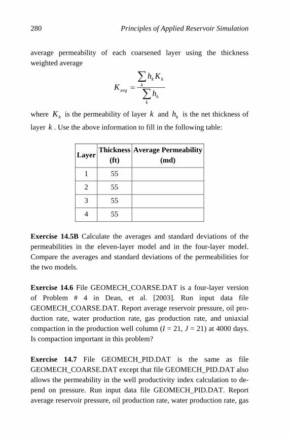
280 Principles of Applied Reservoir Simulation
average permeability of each coarsened layer using the thickness weighted average
∑∑
=
kk
kkk
avg h
KhK
where kK is the permeability of layer k and kh is the net thickness of
layer k . Use the above information to fill in the following table:
LayerThickness
(ft) Average Permeability
(md)
1 55
2 55
3 55
4 55
Exercise 14.5B Calculate the averages and standard deviations of the permeabilities in the eleven-layer model and in the four-layer model. Compare the averages and standard deviations of the permeabilities for the two models. Exercise 14.6 File GEOMECH_COARSE.DAT is a four-layer version of Problem # 4 in Dean, et al. [2003]. Run input data file GEOMECH_COARSE.DAT. Report average reservoir pressure, oil pro-duction rate, water production rate, gas production rate, and uniaxial compaction in the production well column (I = 21, J = 21) at 4000 days. Is compaction important in this problem? Exercise 14.7 File GEOMECH_PID.DAT is the same as file GEOMECH_COARSE.DAT except that file GEOMECH_PID.DAT also allows the permeability in the well productivity index calculation to de-pend on pressure. Run input data file GEOMECH_PID.DAT. Report average reservoir pressure, oil production rate, water production rate, gas

Rock Properties 281
production rate, and uniaxial compaction in the production well column (I = 21, J = 21) at 4000 days. Is pressure-dependent permeability impor-tant in this problem?
282
Chapter 15
Distributing Rock Properties Reservoir rock properties are distributed by contouring and digi-tizing geologic maps. The mapping-contouring process is the point where the geological and geophysical interpretations have their greatest impact on the final representation of the reservoir. This chapter discusses methods for distributing rock properties.
15.1 Types of Flow Models The distribution of rock properties depends on the type of flow model that will be used. Flow models may be classified into three differ-ent types: full field models, sector or window area models, and conceptual models. Full field models are used to match performance of the entire field. They take into account the interaction between all wells and layers. The disadvantage of using full field models is that the num-ber of gridblocks may need to be large or the grid size may need to be relatively coarse to include the entire field. Sector or window area models are designed to look at smaller areas of the field. In the following, we use the term window area model as a synonym for both sector models and window area models. Window area models are often constructed from a full field description. They al-low finer grid resolution or shorter turnaround time if the model runs faster than a full field model. The window area models are useful for

Distributing Rock Properties 283
studying recovery mechanisms and for determining reasonable grid preparation criteria for use in full field models, especially with regard to layering. Full field models require sufficient layering to track fluid con-tact movement or other depth dependent information that is needed to achieve study objectives. Window area models have the disadvantage of not being able to model flux accurately across window area boundaries. This means that effects of wells outside the window area are not ac-counted for except through boundary conditions. Some commercial simulators will output time-dependent boundary conditions for use in window area models. Although this information is helpful, the process is does not necessarily yield accurate results. Field history can be used to guide development of the window area model, but has only limited util-ity as a criterion for validating window model performance. Heinemann [1995] has discussed further concepts and applications of a dynamic win-dowing technique that is designed to minimize the difficulties of preparing and applying window area models in conjunction with full field models. One of the most useful types of models is the conceptual model. Conceptual models can be built quickly and require only an approximate description of the part of the reservoir that is relevant to the conceptual study. Computer resource requirements are relatively small when com-pared with full field or window area models. Results of the conceptual model are qualitative and best used for comparing concepts such as ver-tical layering. They can also be used to prepare pseudo curves for use in full field or window area models. For example, the saturation of a grid-block in a model with a transition zone depends on the depth of the centerpoint of the gridblock. As a result, a grid that is vertically coarse may have only a rough approximation of the transition zone. More accu-rate modeling of saturation gradient in a transition zone requires vertical grid refinement or use of pseudo curves. Conceptual models are useful for preparing such pseudo curves. The disadvantage to conceptual mod-els is that their results do not apply directly to the description of a particular field. Since there is no history match, conceptual model results should be viewed as qualitative rather than quantitative estimates of field
284 Principles of Applied Reservoir Simulation
performance. They do provide useful qualitative information that can be applied to specific fields in window area and full field models.
15.2 Traditional Mapping The different parameters that must be digitized for use in a grid include elevations or structure tops, permeability in three orthogonal di-rections, porosity, gross thickness, net-to-gross thickness, and where appropriate, descriptions of faults, fractures, and aquifers. The resulting maps are digitized by overlaying a grid on the maps and reading a value for each gridblock. The digitizing process is sketched in Figures 15-1a through 15-1d. Several authors have discussed mapping and reservoir characterization, including Harris [1975], Harpole [1985], Haldorsen and Damsleth [1993], Uland, et al. [1997], and Tearpock, et al. [2002]. The resolution of the model depends on the resolution of the grid. A fine grid divides the reservoir into many small gridblocks. It gives the most accurate numerical representation, but has the greatest computational expense. A coarse grid has fewer gridblocks, but the coarse gridblocks must be larger than the fine gridblocks to cover the same model volume. As a result, the coarse grid is less expensive to run than a fine grid, but it is also less accurate numerically. The loss of accu-racy is most evident when a coarse grid is used to model the interface between phases such as fluid contacts and displacement fronts. Thus, fine grid modeling is often the preferred choice to achieve maximum numerical accuracy. It is important to recognize, however, that a fine grid covering an area defined by sparse data can give the illusion of ac-curacy. Sensitivity studies can help quantify the uncertainty associated with the model study. The gridding process is most versatile when used with an inte-grated 3-D reservoir mapping package. Modern mapping techniques include computer generated maps that can be changed relatively quickly once properly set up. The next section introduces computer generated mapping techniques.
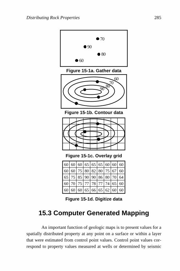
Distributing Rock Properties 285
70
90
6080
Figure 15-1a. Gather data
9080
7060
Figure 15-1b. Contour data
Figure 15-1c. Overlay grid
60 60 60 65 65 65 60 60 60
60 60 75 80 82 80 75 67 60
65 75 85 90 90 86 80 70 64
60 70 75 77 78 77 74 65 60
60 60 60 65 66 65 62 60 60
Figure 15-1d. Digitize data
15.3 Computer Generated Mapping
An important function of geologic maps is to present values for a spatially distributed property at any point on a surface or within a layer that were estimated from control point values. Control point values cor-respond to property values measured at wells or determined by seismic
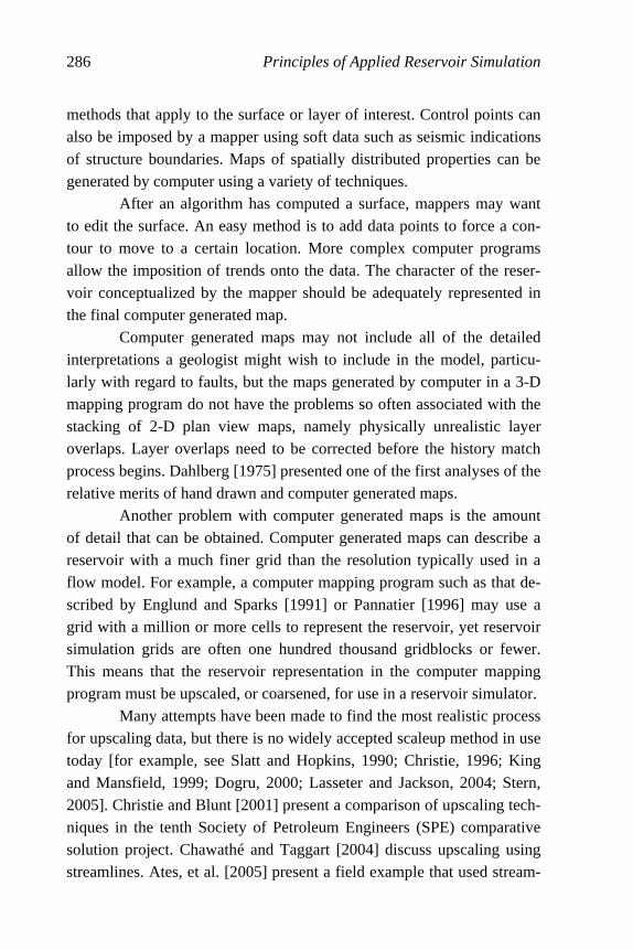
286 Principles of Applied Reservoir Simulation
methods that apply to the surface or layer of interest. Control points can also be imposed by a mapper using soft data such as seismic indications of structure boundaries. Maps of spatially distributed properties can be generated by computer using a variety of techniques. After an algorithm has computed a surface, mappers may want to edit the surface. An easy method is to add data points to force a con-tour to move to a certain location. More complex computer programs allow the imposition of trends onto the data. The character of the reser-voir conceptualized by the mapper should be adequately represented in the final computer generated map. Computer generated maps may not include all of the detailed interpretations a geologist might wish to include in the model, particu-larly with regard to faults, but the maps generated by computer in a 3-D mapping program do not have the problems so often associated with the stacking of 2-D plan view maps, namely physically unrealistic layer overlaps. Layer overlaps need to be corrected before the history match process begins. Dahlberg [1975] presented one of the first analyses of the relative merits of hand drawn and computer generated maps. Another problem with computer generated maps is the amount of detail that can be obtained. Computer generated maps can describe a reservoir with a much finer grid than the resolution typically used in a flow model. For example, a computer mapping program such as that de-scribed by Englund and Sparks [1991] or Pannatier [1996] may use a grid with a million or more cells to represent the reservoir, yet reservoir simulation grids are often one hundred thousand gridblocks or fewer. This means that the reservoir representation in the computer mapping program must be upscaled, or coarsened, for use in a reservoir simulator.
Many attempts have been made to find the most realistic process for upscaling data, but there is no widely accepted scaleup method in use today [for example, see Slatt and Hopkins, 1990; Christie, 1996; King and Mansfield, 1999; Dogru, 2000; Lasseter and Jackson, 2004; Stern, 2005]. Christie and Blunt [2001] present a comparison of upscaling tech-niques in the tenth Society of Petroleum Engineers (SPE) comparative solution project. Chawathé and Taggart [2004] discuss upscaling using streamlines. Ates, et al. [2005] present a field example that used stream-
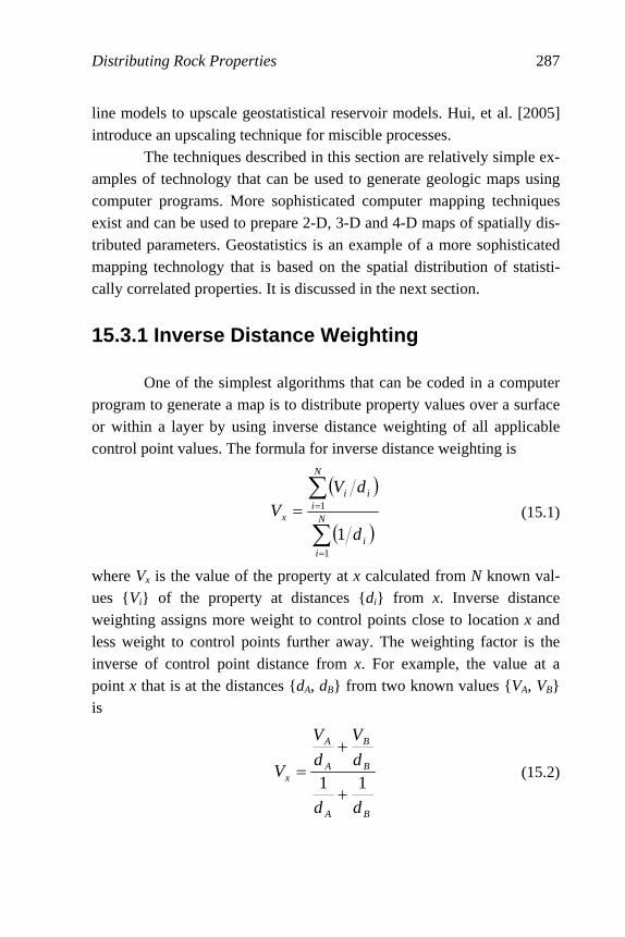
Distributing Rock Properties 287
line models to upscale geostatistical reservoir models. Hui, et al. [2005] introduce an upscaling technique for miscible processes.
The techniques described in this section are relatively simple ex-amples of technology that can be used to generate geologic maps using computer programs. More sophisticated computer mapping techniques exist and can be used to prepare 2-D, 3-D and 4-D maps of spatially dis-tributed parameters. Geostatistics is an example of a more sophisticated mapping technology that is based on the spatial distribution of statisti-cally correlated properties. It is discussed in the next section.
15.3.1 Inverse Distance Weighting
One of the simplest algorithms that can be coded in a computer program to generate a map is to distribute property values over a surface or within a layer by using inverse distance weighting of all applicable control point values. The formula for inverse distance weighting is
( )
( )∑
∑
=
==N
ii
N
iii
x
d
dVV
1
1
1 (15.1)
where Vx is the value of the property at x calculated from N known val-ues {Vi} of the property at distances {di} from x. Inverse distance weighting assigns more weight to control points close to location x and less weight to control points further away. The weighting factor is the inverse of control point distance from x. For example, the value at a point x that is at the distances {dA, dB} from two known values {VA, VB} is
BA
B
B
A
A
x
dd
d
V
d
V
V11
+
+= (15.2)

288 Principles of Applied Reservoir Simulation
Figure 15-2 illustrates the inverse distance weighting example in Equa-tion (15.2) with two control points. If only one value VC is known (N = 1), then Vx = VC for all values of x.
A X
B
Figure 15-2. Inverse Distance Weighting with Two Control Points {A, B}
15.3.2 Weighted Averaging Inverse distance weighting is an example of a technique that uses control points in the neighborhood of an unknown point to estimate the property value at the point. A more general expression for distributing an attribute using a weighted average is
( )
( )∑
∑
=
=
•=
N
ii
i
N
ii
avg
RrW
ZRrWZ
1
1
,
, (15.3)
where
Zavg = weighted average value of attribute Z
Zi = value of attribute Z at control point i
W = weighting function
r i = distance from the interpolated point to control point i
R = user specified search radius
N = number of control points
The search radius R constrains the number of control points N that are used to determine the weighted average of the attribute. An example of a

Distributing Rock Properties 289
weighting function is that in Eq. (15.1), namely 1/di. Another example of a weighting function with a search radius is
( )x
r
R
R
rRrW ⎟
⎠⎞
⎜⎝⎛•⎟
⎠⎞
⎜⎝⎛ −=
2
1, (15.4)
where the value of the exponent x is entered by the user.
15.3.3 Trend Surface Analysis A technique for determining the spatial distribution of a property by computer is to fit a surface through the control points. This technique is referred to as trend surface analysis. Linear trend surface analysis uses regression to fit a line through all control point values in a given direc-tion. The regression model for linear trend surface analysis is
loclocobs yaxaaZ 210 ++= (15.5)
where obsZ is the observed value of attribute Z at the control point,
{ }locloc y,x are the {x -axis, y -axis} locations of the control point, and
{ }210 ,, aaa are regression coefficients. Equation (15.5) can be extended
to be a quadratic function of control point location. Quadratic trend sur-face analysis can fit a curved surface to data, and is therefore useful for representing geologic structures such as anticlines or synclines.
15.4 Geostatistics and Kriging The spatial distribution of rock properties is a fundamental as-pect of the reservoir characterization process. Two modern methods for spatially distributing rock properties are reservoir geophysics (see Chap-ter 12) and geostatistics. Information obtained from reservoir geophysics is improving our ability to “see” between wells in a deterministic sense. By contrast, geostatistics provides a reservoir characterization that is sta-tistical. Many modelers view geostatistics as the method of choice for sophisticated reservoir flow modeling [for example, see Lieber, 1996;

290 Principles of Applied Reservoir Simulation
Haldorsen and Damsleth, 1993; and Rossini, et al., 1994]. Are these methods competing or complementary? This section presents several points about geostatistics that can help answer this question.
Geostatistics is a branch of “applied statistics” that attempts to describe the distribution of a property in space. Geostatistics is also known as spatial statistics. It assumes that a spatially distributed property exhibits some degree of continuity. Porosity and permeability are exam-ples of spatially dependent properties that are suitable for geostatistical description. Much of our discussion of geostatistics is based on publica-tions by Isaaks and Srivastava [1989], Hirsche, et al. [1997], Deutsch and Journel [1998], Chambers, et al. [2000], and Clark and Harper [2002]. Geostatistics consists of a set of mathematical tools which em-ploy the assumption that properties are correlated in space and are not randomly distributed. The geological context of the data must be consid-ered in addition to spatial relationships between data. Geostatistical algorithms provide formalized methods for integrating data of diverse type, quality and quantity. A geostatistical analysis has several goals, including: Ü Acquiring an understanding of the spatial relationships and correla-
tions between reservoir properties; Ü Modeling those relationships with mathematical expressions; Ü Developing an understanding of the uncertainty associated with the
reservoir properties and the conceptual geologic model; and Ü Determining if a deterministic or stochastic approach is appropriate
for the creation of a reservoir model. A deterministic model is a single realization, or representation, of reservoir geology. The uncertainty associated with a deterministic model can be estimated by estimating the sensitivity of the model to un-certainties in available data. A stochastic model is a set of realizations obtained from the probability distributions developed during the geostatistical analysis of data. The shape of a probability distribution is defined by the proximity

Distributing Rock Properties 291
and quality of local data within the context of a spatial correlation model. By its nature, stochastic modeling propagates the uncertainty of the input parameters. Stochastic modeling has two goals. The first goal is to preserve the heterogeneity inherent in a geological system as a means of creating more realistic and useful simulation models. The second goal is to quan-tify the uncertainty in the geologic model by generating many possible realizations. The stochastic model should incorporate multiple data types with varying degrees of quality and quantity. The data should represent different measurement scales. The process of preparing a geologic model requires the devel-opment of a structural and stratigraphic framework using available seismic and well data. Multiple realizations may be generated and used to quantify uncertainty in the geologic model. The process of translating point observations to a conceptual geologic model is a sequential proc-ess. It is also an iterative process if a match of time-dependent (dynamic) data is included in the preparation of the final reservoir model. Once the framework exists, a lithofacies model and petrophysical properties can be incorporated in the flow model.
15.4.1 Geostatistical Modeling
Geostatistical modeling refers to the procedure for determining a set of reservoir realizations. The realizations depend on both the spatial relationships between data points and their statistical correlation as a function of separation in space.
The spatial relationship(s) associated with data are computed and then modeled. This process is analogous to (1) plotting data on a cross-plot (computing) and then (2) fitting a line to the data with linear regression (modeling). The plotted points make up the experimental semi-variogram, and the line that is fit to the data points is called the semi-variogram model. Figure 15-3 illustrates a fit to data by a semi-variogram model.
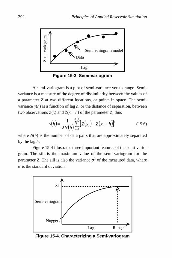
292 Principles of Applied Reservoir Simulation
Sem
i-va
r iog
ram
Semi-variogram model
Data
Lag
Figure 15-3. Semi-variogram A semi-variogram is a plot of semi-variance versus range. Semi-variance is a measure of the degree of dissimilarity between the values of a parameter Z at two different locations, or points in space. The semi-
variance γ(h) is a function of lag h, or the distance of separation, between
two observations Z(x) and Z(x + h) of the parameter Z, thus
( ) ( ) ( ) ( )[ ]( )
∑=
+−=γhN
iii hxZxZ
hNh
1
2
2
1(15.6)
where N(h) is the number of data pairs that are approximately separated by the lag h. Figure 15-4 illustrates three important features of the semi-vario-gram. The sill is the maximum value of the semi-variogram for the
parameter Z. The sill is also the variance σ2 of the measured data, where
σ is the standard deviation.
Semi-variogram
Lag Range
Nugget
Sill
Figure 15-4. Characterizing a Semi-variogram
Distributing Rock Properties 293
The nugget in Figure 15-4 is the value of the semi-variance at zero lag. A nonzero value of the nugget is due to factors such as sam-pling error and short range variability of the parameter. In fact, the term “nugget” refers to the observation that the lag for a finite size gold nug-get can never equal zero. The range in Figure 15-4 is an estimate of the maximum correla-tion length between two points at a separation distance h. A spatial correlation between values of parameter Z exists at values of the lag less than the range. Several types of semi-variogram models exist. For example, the exponential model is
( )⎭⎬⎫
⎩⎨⎧
⎟⎠⎞
⎜⎝⎛−−+=γ
a
hCCh exp110 (15.7)
and the Gaussian model is
( )⎭⎬⎫
⎩⎨⎧
⎟⎟⎠
⎞⎜⎜⎝
⎛−−+=γ
2
2
10 exp1a
hCCh (15.8)
where 0≥h is lag, 0C is the nugget, 1C is the sill, and a is the range
of influence. Semi-variogram modeling is performed by fitting a semi-
variogram model to experimental data as in Figure 15-3. The resulting semi-variogram is a measure of the spatial dependence of reservoir at-tributes such as porosity, permeability and net thickness. The semi-variogram model is used to predict values of the modeled attribute at unsampled locations.
One widely used estimation technique is kriging. Kriging is named after the South African mining engineer D.G. Krige who helped pioneer the development of geostatistical methods in the 1950’s. Kriging is a linear weighted average method. The weights used in kriging are based on the semi-variogram model of spatial correlation. It is instructive to make these points explicit.

294 Principles of Applied Reservoir Simulation
The kriging equation for estimating the value of attribute PZ at
point P from a set of n control points with attribute values
{ }niZi ,,2,1: K= is
∑=
=n
iiiP ZwZ
1
(15.9)
The attribute PZ may be a rock property such as porosity or permeabil-
ity. The weights { }niwi ,,2,1: K= are calculated from the set of n
equations
( ) ( ) ( ) ( )( ) ( ) ( ) ( )
( ) ( ) ( ) ( )nPnnnnn
Pnn
Pnn
hhwhwhw
hhwhwhw
hhwhwhw
γ=λ+γ++γ+γ
γ=λ+γ++γ+γγ=λ+γ++γ+γ
L
M
L
L
2211
22222211
11122111
(15.10)
The semi-variogram ( )ijhγ is the semi-variogram at lag distance ijh be-
tween two points ( )ji PP , . The semi-variogram ( )iPhγ is the semi-
variogram at lag distance iPh between control point iP and the point P
where attribute PZ is being estimated. The constant λ is the Lagrange
multiplier for the “unbiased” constraint
11
=∑=
n
iiw (15.11)
Equation (15.9) is considered the “best linear unbiased estimate”
(BLUE) of PZ , and the procedure for solving the above set of equations
is considered ordinary kriging. Universal kriging combines ordinary kriging and trend surface analysis.
15.4.2 Technical Note The ordinary kriging equations in Eq. (15.10) and (15.11) are
1+n equations for the n weights { }niwi ,,2,1: K= and the Lagrange
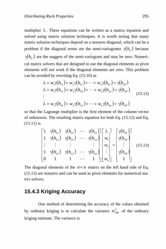
Distributing Rock Properties 295
multiplier λ . These equations can be written as a matrix equation and
solved using matrix solution techniques. It is worth noting that many matrix solution techniques depend on a nonzero diagonal, which can be a
problem if the diagonal terms are the semi-variograms ( )iihγ because
( )iihγ are the nuggets of the semi-variogram and may be zero. Numeri-
cal matrix solvers that are designed to use the diagonal elements as pivot elements will not work if the diagonal elements are zero. This problem can be avoided by rewriting Eq. (15.10) as
( ) ( ) ( ) ( )( ) ( ) ( ) ( )
( ) ( ) ( ) ( )nPnnnnn
Pnn
Pnn
hhwhwhw
hhwhwhw
hhwhwhw
γ=γ++γ+γ+λ
γ=γ++γ+γ+λγ=γ++γ+γ+λ
L
M
L
L
2211
22222211
11122111
(15.12)
so that the Lagrange multiplier is the first element of the column vector of unknowns. The resulting matrix equation for both Eq. (15.12) and Eq. (15.11) is
( ) ( ) ( )( ) ( ) ( )
( ) ( ) ( )
( )( )
( )⎥⎥⎥⎥⎥⎥
⎦
⎤
⎢⎢⎢⎢⎢⎢
⎣
⎡
γ
γγ
=
⎥⎥⎥⎥⎥⎥
⎦
⎤
⎢⎢⎢⎢⎢⎢
⎣
⎡ λ
⎥⎥⎥⎥⎥⎥
⎦
⎤
⎢⎢⎢⎢⎢⎢
⎣
⎡
γγγ
γγγγγγ
11110
1
1
1
2
1
2
1
21
22221
11211
nP
P
P
n
nnnn
n
n
h
h
h
w
w
w
hhh
hhh
hhh
M
M
L
L
MMMM
L
L
(15.13)
The diagonal elements of the nn× matrix on the left hand side of Eq.
(15.13) are nonzero and can be used as pivot elements for numerical ma-trix solvers.
15.4.3 Kriging Accuracy
One method of determining the accuracy of the values obtained
by ordinary kriging is to calculate the variance 2OKσ of the ordinary
kriging estimate. The variance is

296 Principles of Applied Reservoir Simulation
( ) ( )PP
n
iiPiOK hhw γ−λ+γ=σ ∑
=1
2 (15.14)
where the Lagrange multiplier is
( ) ( )∑∑∑= ==
γ−γ=λn
i
n
jijji
n
iiPi hwwhw
1 11
(15.15)
Equations (15.14) and (15.15) can be solved once the weights have been calculated. Equation (15.15) can be used to check the value of the La-grange multiplier obtained by solving Eq. (15.13).
Another method of determining the accuracy of the values ob-tained by an estimation technique is to treat a sampled (known) data point as an unknown point at the test location. The estimation technique is used to calculate the parameter at the test location and the resulting value is compared with the known data point. The accuracy of the esti-mation process can be quantified by calculating the semi-variance of actual values relative to the estimated values. The resulting semi-variance provides a cross-validation of the original semi-variogram model and provides information about the quality of the estimation tech-nique. Notice that this model cross-validation procedure could be applied to any computer based estimation technique.
15.4.4 The Use and Abuse of Geostatistics Hirsche, et al. [1997; page 259] have pointed out that “geostatis-tical reservoir characterization should not be done in isolation.” Geostatistics is like other reservoir characterization techniques: the tech-nique is most successful when all available data is incorporated into the reservoir characterization process. The violation of basic geostatistical assumptions can lead to the creation of an inaccurate reservoir model. Inaccuracies in the model ap-pear as errors in associated maps. Limited well control and biased sampling of well information are examples of real world constraints that can violate the underlying assumptions of geostatistics. Abrupt changes
Distributing Rock Properties 297
in reservoir features, such as faults and high permeability channels, are difficult to identify using geostatistics [Fanchi, et al., 1996]. Geostatistics and stochastic modeling can be used to integrate data, provide a realistic representation of reservoir heterogeneity, and quantify uncertainty. On the other hand, the existence of multiple realiza-tions can be confusing and more expensive than the construction of a single deterministic representation of the reservoir. In addition, the sto-chastic images may look realistic but actually do a poor job of representing flow in the actual reservoir. The process of validating the reservoir model is made more complicated by the existence of multiple realizations.
15.5 Geostatistical Case Study An example of a full field model study using a geostatistical res-ervoir realization is the reservoir management study of the N.E. Nash Unit in Oklahoma [Fanchi, et al., 1996]. The goal of the study was to prepare a full field reservoir flow model that could be used to identify unswept parts of the field. We knew from the history of the field that water was breaking through at several wells. The study was designed to look for places where an additional production well could be economi-cally drilled. The N.E. Nash Unit has a gradual dip from north to south. The Misener sandstone reservoir is bounded above by the Woodford shale, on the flanks by the Sylvan shale, and below by the Viola limestone. The Viola limestone does allow some aquifer support for the Misener sand-stone. One of the primary tasks of the study was to map the N.E. Nash Unit. Two sets of maps were prepared: conventional hand-drawn maps, and a set of maps based on a geostatistical analysis of the field. The hand-drawn maps correspond to the deterministic approach in which a single realization is used, while the geostatistical maps correspond to a stochastic image of the reservoir.

298 Principles of Applied Reservoir Simulation
A geostatistical analysis was performed using forty-two well control points to calculate structural tops, gross thickness, net-to-gross ratio, and porosity. A crossplot between porosity and core permeability yielded a relationship for calculating permeability from porosity. From this data, directional semi-variograms were prepared to describe the spa-tial continuity of each parameter.
When two sets of maps were compared, the hand-drawn maps were found to be more homogenous than the geostatistical maps. The geostatistical maps exhibited the large scale trends shown in the hand-drawn maps, but contained more local variability. This was not surpris-ing, since additional heterogeneity is expected to arise as a result of geostatistical mapping. The choice of final maps was based on management priorities: minimize the risk of drilling a dry hole on the flanks of the field, and complete the study before water breakthrough occurred in the remaining oil producers. The geostatistical model satisfied both of these criteria. The main flow path in the reservoir was narrower in the geostatistically generated maps than in the hand-drawn maps, and the geostatistical re-alization could be modified more quickly than hand-drawn maps. Once a set of maps was chosen, the history matching process could begin. Tracer information in the form of salinity changes helped identify sources of injection water as the water was produced. This was valuable in defining flow channels that could not otherwise be inferred. In some areas, transmissibility and porosity changes were needed to match water cut and reservoir pressure. The geostatistical realization used in the N.E. Nash study was just a single realization. It was selected because it satisfied constraints imposed by previous volumetric and material balance studies. If these constraints had not been available or had been less reliable, which would be the case early in the life of a field, a geostatistical study would require the use of multiple realizations to characterize the reservoir. This raises the question of how many realizations are necessary. Figure 15-5 shows a random sampling from a discrete probabil-ity distribution. A running average is calculated as the average of all preceding trials. For example, the running average at trial 10 is obtained

Distributing Rock Properties 299
by averaging the first 10 trial results. The running average shown in Fig-ure 15-5 does not stabilize, or approach a constant value, until at least twenty trials have been completed. This is a large number of realizations if history matching is needed for each realization. Indeed, it would be an unacceptably large number of realizations, in most cases, because of the time it takes to perform a history match. Most studies are usually based on the assumption that a single history match will be sufficient.
Trial
Pro
pert
y V
alue
Value Avg
Figure 15-5. Running Average Multiple realizations can also confuse people who are not closely involved with the modeling process because they do not have a single picture of the reservoir. On the other hand, the use of multiple re-alizations makes it possible to quantify the uncertainty associated with our limited knowledge of properties distributed spatially throughout the field.
Table 15-1 summarizes the advantages and concerns associated with geostatistics. There is no established procedure for selecting one or more realizations for history matching from a set of geostatistically de-rived realizations. Examples of procedures are described by Rossini, et al. [1994] and Gilman, et al. [2002]. Applications of reservoir geostatis-tics in the context of a multidisciplinary study are presented by several authors, such as Wang, et al. [1998] and Dubrule [2003].

300 Principles of Applied Reservoir Simulation
Table 15-1 Geostatistics
Advantages Concerns
Ü Realism Ü Quantification of
uncertainty
Ü Multiple realizations entail cost and con-fusion
Ü History matching still necessary to ac-count for model discontinuities such as channeling
Ü History matching complicated by factors such as probabilistically generated heter-ogeneity
Exercises Exercise 15.1 Sketch the model grids for data files EXAM1.DAT, EXAM2.DAT, EXAM3.DAT, EXAM5.DAT, and EXAM7.DAT using the information from each data file. Exercise 15.2 Sketch the model grids for case study data files CS-MB.DAT, CS-VC.DAT, and CS-XS.DAT using the information from each data file. Exercise 15.3 Modify the grid in EXAM3.DAT so that it has only ten gridblocks in the x direction, but the model volume is unchanged. Be sure to relocate the wells relative to the grid to keep them in their appro-priate physical locations and correct the PID index. How does the coarser grid affect the model?
Exercise 15.4 Modify the grid in EXAM2.DAT so that it has 5 × 5 × 4 gridblocks. The well should be in the center of the reservoir and the res-ervoir volume should be unchanged by the redefinition of the grid. Correct the PID index. How does the finer grid affect model performance when the model is run for three years?
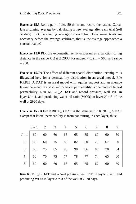
Distributing Rock Properties 301
Exercise 15.5 Roll a pair of dice 50 times and record the results. Calcu-late a running average by calculating a new average after each trial (roll of dice). Plot the running average for each trial. How many trials are necessary before the average stabilizes, that is, the average approaches a constant value? Exercise 15.6 Plot the exponential semi-variogram as a function of lag
distance in the range 20000 ≤≤ h for nugget = 0, sill = 500, and range
= 200. Exercise 15.7A The effect of different spatial distribution techniques is illustrated here for a permeability distribution in an areal model. File KRIGE_A.DAT is an areal model with aquifer support and an average lateral permeability of 75 md. Vertical permeability is one tenth of lateral permeability. Run KRIGE_A.DAT and record pressure, well PID in layer K = 1, and producing water-oil ratio (WOR) in layer K = 3 of the well at 2920 days. Exercise 15.7B File KRIGE_B.DAT is the same as file KRIGE_A.DAT except that lateral permeability is from contouring in each layer, thus:
I = 1 2 3 4 5 6 7 8 9
J = 1 60 60 60 65 65 65 60 60 60
2 60 60 75 80 82 80 75 67 60
3 65 75 85 90 90 86 80 70 64
4 60 70 75 77 78 77 74 65 60
5 60 60 60 65 65 65 62 60 60
Run KRIGE_B.DAT and record pressure, well PID in layer K = 1, and producing WOR in layer K = 3 of the well at 2920 days.
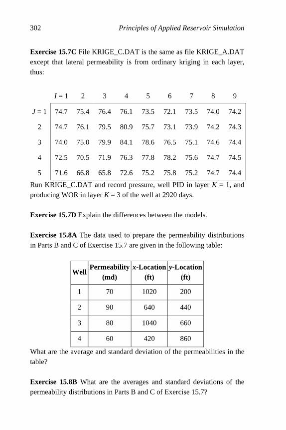
302 Principles of Applied Reservoir Simulation
Exercise 15.7C File KRIGE_C.DAT is the same as file KRIGE_A.DAT except that lateral permeability is from ordinary kriging in each layer, thus:
I = 1 2 3 4 5 6 7 8 9
J = 1 74.7 75.4 76.4 76.1 73.5 72.1 73.5 74.0 74.2
2 74.7 76.1 79.5 80.9 75.7 73.1 73.9 74.2 74.3
3 74.0 75.0 79.9 84.1 78.6 76.5 75.1 74.6 74.4
4 72.5 70.5 71.9 76.3 77.8 78.2 75.6 74.7 74.5
5 71.6 66.8 65.8 72.6 75.2 75.8 75.2 74.7 74.4
Run KRIGE_C.DAT and record pressure, well PID in layer K = 1, and producing WOR in layer K = 3 of the well at 2920 days. Exercise 15.7D Explain the differences between the models. Exercise 15.8A The data used to prepare the permeability distributions in Parts B and C of Exercise 15.7 are given in the following table:
WellPermeability
(md) x-Location
(ft) y-Location
(ft)
1 70 1020 200
2 90 640 440
3 80 1040 660
4 60 420 860
What are the average and standard deviation of the permeabilities in the table? Exercise 15.8B What are the averages and standard deviations of the permeability distributions in Parts B and C of Exercise 15.7?

Distributing Rock Properties 303
Exercise 15.9 Files RIM_2D.DAT and RIM_SYMMETRIC.DAT are 2-D models of gas production from an anticlinal gas reservoir with an oil rim. Run both files and use 3DView to view the structure. Are there any differences between the structures in the two files? Confirm your analy-sis by looking at the structure tops in the data files.
304
Chapter 16
Fluid Properties Properties of petroleum fluids must be quantified in a reservoir simulator. The range of applicability of a reservoir simulator is defined, in part, by the types of fluids that can be modeled using the mathematical algorithms coded in the simulator. This chapter discusses the general types of fluids that may be encountered in a commercial reservoir envi-ronment and that are suitable for flow modeling. For additional information, see Amyx, et al. [1960], Pedersen, et al. [1989], Koederitz, et al. [1989], McCain [1990, 1991], Towler [2002], and Walsh and Lake [2003].
16.1 Fluid Types The elemental composition (by mass) of petroleum is approxi-mately 84% to 87% carbon, 11% to 14% hydrogen, 0.6% to 8% sulphur, 0.02% to 1.7% nitrogen, 0.08% to 1.8% oxygen, and 0% to 0.14% met-als. The composition of petroleum shows that petroleum fluids are predominantly hydrocarbons. The most common hydrocarbon molecules are paraffins, napthenes, and aromatics because of the relative stability of the molecules. A paraffin is a saturated hydrocarbon, that is, it has a sin-gle bond between carbon atoms. Examples include methane and ethane.
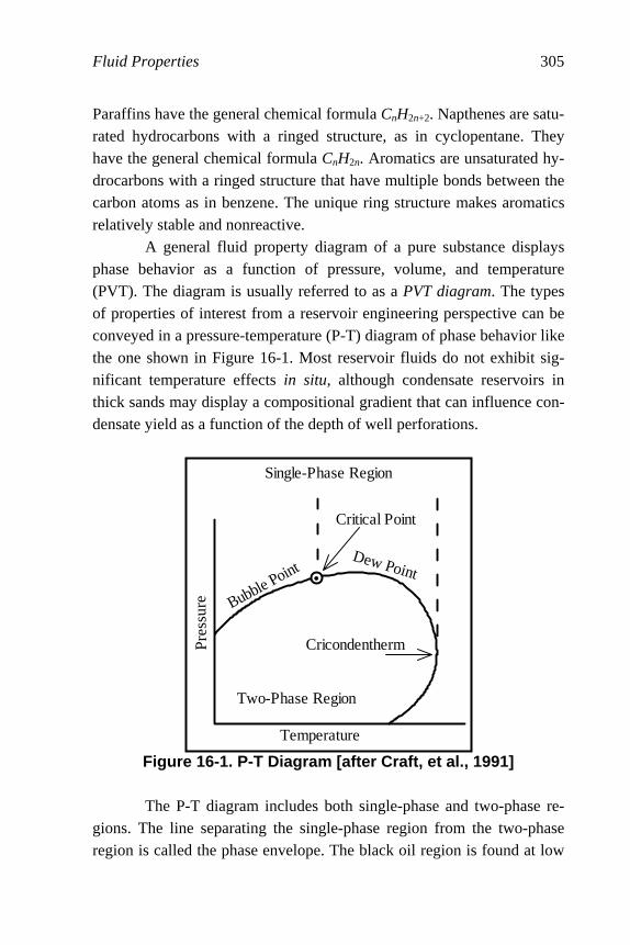
Fluid Properties 305
Paraffins have the general chemical formula CnH2n+2. Napthenes are satu-rated hydrocarbons with a ringed structure, as in cyclopentane. They have the general chemical formula CnH2n. Aromatics are unsaturated hy-drocarbons with a ringed structure that have multiple bonds between the carbon atoms as in benzene. The unique ring structure makes aromatics relatively stable and nonreactive. A general fluid property diagram of a pure substance displays phase behavior as a function of pressure, volume, and temperature (PVT). The diagram is usually referred to as a PVT diagram. The types of properties of interest from a reservoir engineering perspective can be conveyed in a pressure-temperature (P-T) diagram of phase behavior like the one shown in Figure 16-1. Most reservoir fluids do not exhibit sig-nificant temperature effects in situ, although condensate reservoirs in thick sands may display a compositional gradient that can influence con-densate yield as a function of the depth of well perforations.
Figure 16-1. P-T Diagram [after Craft, et al., 1991]
The P-T diagram includes both single-phase and two-phase re-gions. The line separating the single-phase region from the two-phase region is called the phase envelope. The black oil region is found at low
Two-Phase Region
Cricondentherm
Temperature
Pre
ssur
e Bubble Point
•
Single-Phase Region
Critical Point
Dew Point

306 Principles of Applied Reservoir Simulation
temperature and in the high pressure region above the bubble point curve separating the single-phase and two-phase regions. If we consider pres-sures in the single-phase region and move to the right of the diagram by letting temperature increase towards the critical point, we encounter volatile oils. At temperatures above the critical point but less than the cricondentherm – the maximum temperature of the phase envelope – reservoir fluids behave like condensates. When reservoir temperature is greater than the cricondentherm, we encounter only the gas phase.
Table 16-1 summarizes fluid types. Notice that separator gas-oil ratio (GOR) is a useful indicator of fluid type.
Table 16-1 Rules of Thumb for Classifying Fluid Types
Fluid Type
Separator GOR(MSCF/STB)
Pressure Depletion Behavior in Reservoir
Dry gas No surface liquids Remains gas
Wet gas > 100 Remains gas
Condensate 3 − 100 Becomes gas with liquid drop out
Volatile oil 1.5 − 3 Becomes liquid with significant gas
Black oil 0.1 − 1.5 Becomes liquid with some gas
Heavy oil ∼ 0 Exhibits negligible gas formation
Let us consider a reservoir containing hydrocarbons that are at a pressure and temperature corresponding to the single-phase black oil re-gion. If reservoir pressure declines at constant temperature, the reservoir pressure will eventually cross the bubble point pressure curve and enter the two-phase gas-oil region. Similarly, starting with a single-phase con-densate and letting reservoir pressure decline at constant temperature, the reservoir pressure will cross the dew point pressure curve to enter the two-phase region. In this case, a free-phase liquid drops out of the con-densate gas. Once liquid drops out, it is very difficult to recover. One
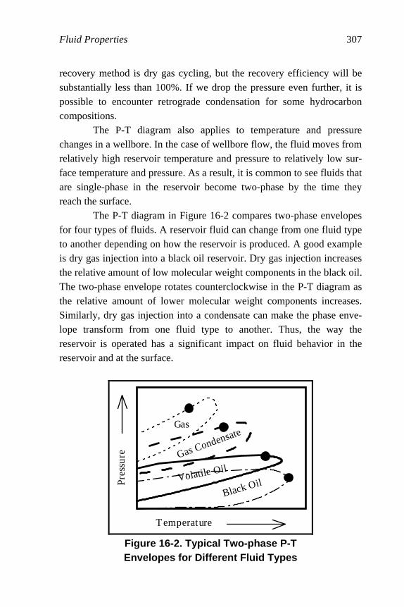
Fluid Properties 307
recovery method is dry gas cycling, but the recovery efficiency will be substantially less than 100%. If we drop the pressure even further, it is possible to encounter retrograde condensation for some hydrocarbon compositions. The P-T diagram also applies to temperature and pressure changes in a wellbore. In the case of wellbore flow, the fluid moves from relatively high reservoir temperature and pressure to relatively low sur-face temperature and pressure. As a result, it is common to see fluids that are single-phase in the reservoir become two-phase by the time they reach the surface. The P-T diagram in Figure 16-2 compares two-phase envelopes for four types of fluids. A reservoir fluid can change from one fluid type to another depending on how the reservoir is produced. A good example is dry gas injection into a black oil reservoir. Dry gas injection increases the relative amount of low molecular weight components in the black oil. The two-phase envelope rotates counterclockwise in the P-T diagram as the relative amount of lower molecular weight components increases. Similarly, dry gas injection into a condensate can make the phase enve-lope transform from one fluid type to another. Thus, the way the reservoir is operated has a significant impact on fluid behavior in the reservoir and at the surface.
Temperature
Pre
ssu
re
Gas
Gas Condensate
Black OilVolatile Oil
Figure 16-2. Typical Two-phase P-T Envelopes for Different Fluid Types

308 Principles of Applied Reservoir Simulation
Table 16-2 shows different compositions for typical fluid types. Dry gas usually contains only the lower molecular weight components. Gas condensates start to add higher molecular weight components. Vola-tile oils continue to add higher molecular weight components. Black oils result from the addition of higher molecular weight components and the reduction of lower molecular weight components. If we monitor methane content (C1), we see that it tends to decrease as fluids change from dry gas to black oil.
Table 16-2 Typical Molar Compositions of Petroleum Fluid Types
[after Pedersen, et al., 1989]
Component Gas Gas Condensate Volatile Oil Black Oil
N2 CO2 C1 C2 C3 iC4+nC4 iC5+nC5 iC6+nC6
0.31.1
90.04.91.91.10.4
C6+: 0.3
0.71 8.65
70.86 8.53 4.95 2.00 0.81 0.46
1.672.18
60.517.524.744.122.971.99
0.672.11
34.937.007.825.483.803.04
C7 C8 C9 C10 C11 C12
0.61 0.71 0.39 0.28 0.20 0.15
2.452.411.691.421.02
C12+: 5.31
4.394.713.211.791.721.74
C13 C14 C15 C16 C17
0.11 0.10 0.07 0.05
C17+: 0.37
1.741.351.341.06
C17+: 12.10

Fluid Properties 309
16.2 Fluid Modeling In general, fluid behavior is best modeled using an equation of state. Table 16-3 shows some cubic equations of state (EoS) used in commercial compositional simulators. In addition to pressure (P), vol-ume (V), and temperature (T), the EoS contains the gas constant R and a set of adjustable parameters {a, b} which may be functions of tempera-ture. The EoS in Table 16-3 are called “cubic” because they yield a cubic equation for the compressibility factor Z = PV/RT. In the case of an ideal gas, Z = 1.
Table 16-3 Examples of Cubic Equations of State
Redlich-Kwong ( )bVV
Ta
bV
RTP
+−
−=
21
Soave-Redlich-Kwong( )
( )bVV
ta
bV
RTP
+−
−=
Peng-Robinson ( )
( ) ( )bVbbVV
ta
bV
RTP
−++−
−=
Zudkevitch-Joffe ( )( )[ ]TbVV
TTa
bV
RTP
+−
−=
21
Equations of state are valuable for representing fluid properties in many situations. For example, suppose we want to model a system in which production is commingled from more than one reservoir with more than one fluid type. In this case the most appropriate simulator would be a compositional simulator because a black oil simulator would not provide as accurate a representation of fluid behavior. The two most common types of reservoir fluid models are black oil models and compositional models. Black oil models are based on the assumption that the saturated phase properties of two hydrocarbon

310 Principles of Applied Reservoir Simulation
phases (oil and gas) depend on pressure only. Compositional models also assume two hydrocarbon phases, but they allow the definition of many hydrocarbon components. Unlike a black oil simulator, which can be thought of as a compositional simulator with two components, a compo-sitional simulator often has six to ten components. By comparison, process engineering simulators that are used to model surface facilities typically require up to twenty components or more. The cost of running a compositional simulator increases dramatically with increases in the number of components modeled, but the additional components make it possible to model complex fluid phase behavior more accurately. If compositional model results are to be used in a process engineering model, it is often necessary to compromise on the number of components to be used for each application. Equations of state must be used to calculate equilibrium relations in a compositional model. This entails tuning parameters such as EoS parameters {a, b} in Table 16-3. Several regression techniques exist for tuning an EoS. They usually differ in the choice of EoS parameters that are to be varied in an attempt to match lab data with the EoS. The use of equations of state in compositional simulation is discussed by several authors, such as Whitson and Brulé [2000], Wang and Pope [2001], and Thomas, et al. [2002].
Figures 16-3 and 16-4 show typical fluid property behavior of gas and oil properties for a black oil model. Gas phase properties are gas formation volume factor (Bg), gas viscosity (µg), and liquid yield (rs). Oil phase properties are oil formation volume factor (Bo), oil viscosity (µo), and solution GOR (Rso). Both saturated and undersaturated curves are included as functions of pressure only. Phase changes occur at the satura-tion pressures. Single-phase oil becomes two-phase gas-oil when pressure drops below the bubble point pressure (Pb), and single-phase gas becomes two-phase gas condensate when pressure drops below the dew point pressure (Pd).
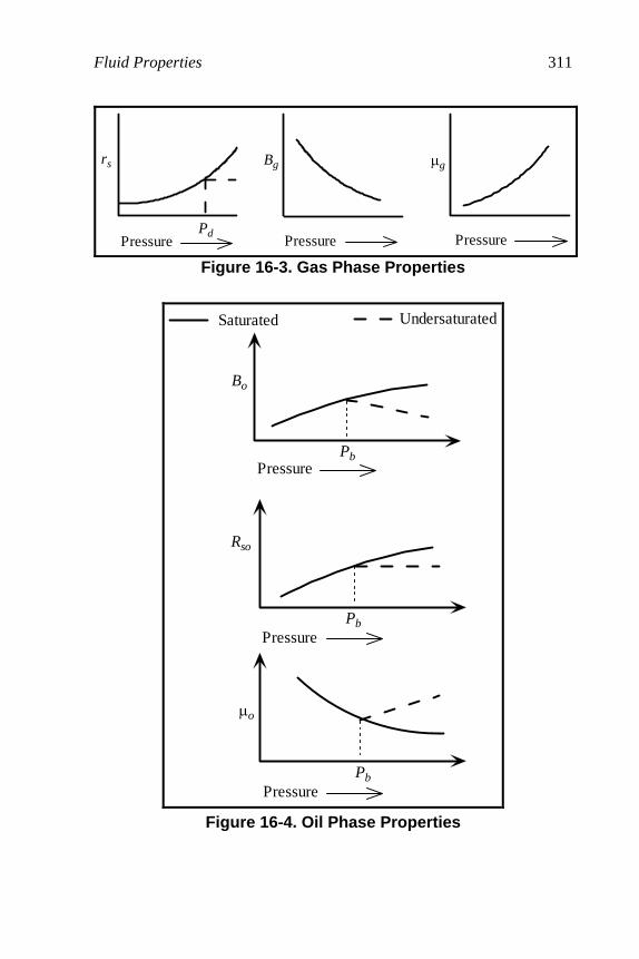
Fluid Properties 311
rs
Pd
Bg µg
Pressure Pressure Pressure
Figure 16-3. Gas Phase Properties
Bo
Pb
Rso
Pressure
Pressure
Pressure
Pb
Pb
µo
Saturated Undersaturated
Figure 16-4. Oil Phase Properties
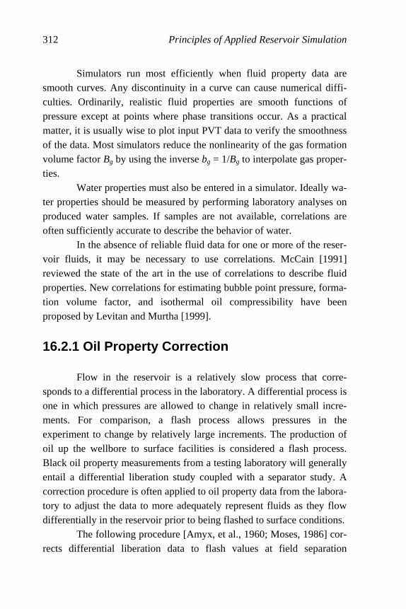
312 Principles of Applied Reservoir Simulation
Simulators run most efficiently when fluid property data are smooth curves. Any discontinuity in a curve can cause numerical diffi-culties. Ordinarily, realistic fluid properties are smooth functions of pressure except at points where phase transitions occur. As a practical matter, it is usually wise to plot input PVT data to verify the smoothness of the data. Most simulators reduce the nonlinearity of the gas formation volume factor Bg by using the inverse bg = 1/Bg to interpolate gas proper-ties. Water properties must also be entered in a simulator. Ideally wa-ter properties should be measured by performing laboratory analyses on produced water samples. If samples are not available, correlations are often sufficiently accurate to describe the behavior of water. In the absence of reliable fluid data for one or more of the reser-voir fluids, it may be necessary to use correlations. McCain [1991] reviewed the state of the art in the use of correlations to describe fluid properties. New correlations for estimating bubble point pressure, forma-tion volume factor, and isothermal oil compressibility have been proposed by Levitan and Murtha [1999].
16.2.1 Oil Property Correction
Flow in the reservoir is a relatively slow process that corre-sponds to a differential process in the laboratory. A differential process is one in which pressures are allowed to change in relatively small incre-ments. For comparison, a flash process allows pressures in the experiment to change by relatively large increments. The production of oil up the wellbore to surface facilities is considered a flash process. Black oil property measurements from a testing laboratory will generally entail a differential liberation study coupled with a separator study. A correction procedure is often applied to oil property data from the labora-tory to adjust the data to more adequately represent fluids as they flow differentially in the reservoir prior to being flashed to surface conditions.
The following procedure [Amyx, et al., 1960; Moses, 1986] cor-rects differential liberation data to flash values at field separation

Fluid Properties 313
conditions. If the separator formation volume factor for oil Bo and solu-tion gas-oil ratio Rso are known, the conversion equations are:
( ) ( )odpb
ofbpodo B
BPBPB = (16.1)
and
( ) ( )( )odpb
ofbpsodsodbpsofbpso B
BPRRRPR −−= (16.2)
where the variable P is pressure. The subscripts in the equations are de-fined as follows: d refers to differential liberation data; f refers to flash data; and bp refers to values at the bubble point pressure. The corrections alter solution gas-oil ratio and oil formation volume factor so that they may be used in black oil simulation. Alternative procedures for adjusting differential liberation data to separator conditions are discussed by Po-etmann and Thompson [1986], McCain [2002], Walsh and Lake [2003], and Al-Marhoun [2003].
16.3 Fluid Sampling All laboratory measurements of fluid properties and subsequent analyses are useless if the fluid samples do not adequately represent in
situ fluids. The goal of fluid sampling is to obtain a sample that is repre-sentative of the original fluid in the reservoir. It is often necessary to condition the well before the sample is taken. A well is conditioned by producing any nonrepresentative fluid, such as drilling mud, from within and around the wellbore until it is replaced by original reservoir fluid flowing into the wellbore. Fluid samples may then be taken from either the surface or subsurface. Subsurface sampling requires lowering a pressurized container to the production interval and subsequently trapping a fluid sample. This is routinely accomplished by drill stem testing, especially when access to surface facilities is limited. Downhole fluid sampling is most effective when fluids flow into the well as a single phase and the fluid samples are
314 Principles of Applied Reservoir Simulation
obtained early in the life of the well. It is generally cheaper and easier to take surface samples from separator gas and oil. If a surface sample is taken, the original in situ fluid, that is, the fluid at reservoir pressure and temperature, must be reconstituted by combining separator gas and separator oil samples. The recombination step assumes that measurements of flow data at the surface are accurate, especially gas-oil ratio. Subsurface sampling from a properly condi-tioned well avoids the recombination step, but is more difficult and costly than surface sampling, and usually provides a smaller volume of sample fluid. The validity of fluid property data depends on the quality of the fluid sampling procedure.
16.4 IFLO Fluid Model
The multicomponent, pseudomiscible simulator IFLO uses the extended fluid properties model described by Ammer, et al. [1991]. It is an adaptation of Chase and Todd’s [1984] mixing parameter method. See Ammer, et al. [1991] or Fanchi [2000] for additional details. Bubble point tracking and the gas property correlation option implemented in IFLO are outlined below.
16.4.1 Bubble Point Tracking The technique of variable switching [Thomas, et al., 1976] is used to track bubble point pressure in IFLO [Ammer, et al. 1991]. The primary variables that specify the state of a gridblock depend on the con-dition of the gridblock. The saturated condition of the gridblock is determined at the beginning of an iteration by comparing oil phase pres-sure and bubble point pressure. At the end of the iteration, saturated gridblocks are tested for a change of state. If gas saturation is positive in the saturated gridblock, bubble point pressure Pb is set equal to gridblock pressure P. If gas saturation is negative, gas saturation is set to zero and Pb is set slightly below the oil phase pressure. This makes the gridblock slightly undersaturated as it enters the next iteration. Undersaturated
Fluid Properties 315
gridblocks do not require any special switching logic. The next iteration is then performed.
16.4.2 Gas PVT Correlation Option The Benedict-Webb-Rubin [1940] eight-parameter equation of state is used to express the Z-factor as a function of pseudocritical tem-perature Tr and pseudocritical pressure Pr, thus Z = Z(Pr,Tr). Once Z is known, the gas formation volume factor is easily determined for a given temperature and pressure using the real gas law. The isothermal gas compressibility cg is
⎥⎥
⎦
⎤
⎢⎢
⎣
⎡
⎟⎟⎠
⎞⎜⎜⎝
⎛
∂∂
−=rTrrc
g P
Z
ZPPc
111 (16.3)
where Pc is the critical pressure (psia). Real gas viscosities are computed using the Carr, Kobayashi, and Burrows [1954] hydrocarbon gas viscosity determination procedure.
16.4.3 Pseudopressure Calculations Pseudopressures are defined by
( ) ∫ ′µ′
=ψP
P go
PdZ
PP 2 (16.4)
where
P′ = dummy integration variable with pressure units (psia)
Po = reference pressure = 14.7 psia
P = specified pressure (psia)
µg = gas viscosity (cp)
Z = gas compressibility factor

316 Principles of Applied Reservoir Simulation
The pseudopressure ψ(P) is often written as m(P). Since µg and Z depend
on P′, evaluation of Eq. (16.4) is accomplished by numerical integration
using the trapezoidal rule and a user-specified pressure increment dP′.
16.4.4 Correlation Range Limits The following range limits apply to correlations used in calculat-ing gas Z-factors, compressibilities and viscosities:
40040
5.155.0
0.1501.0
0.305.1
<<
<<
<<
<<
T
SPG
P
P
T
T
c
c
(16.5)
where
Tc = pseudocritical temperature (oR)
Pc = pseudocritical pressure (psia)
T = temperature (oR)
P = pressure (psia)
SPG= gas specific gravity
No values of T, P, or SPG should be used that exceed the above correla-tion ranges. If the range limit is exceeded, a fatal error will occur.
16.5 Rock-Fluid Interaction Small scale laboratory measurements of fluid flow in porous media show that fluid behavior depends on the properties of the solid material. Laboratory measurements provide information at the core scale (Macro Scale) and, in some cases, at the microscopic scale (Micro Scale). The interaction between rock and fluid is modeled using a variety

Fluid Properties 317
of physical parameters that include relative permeability and capillary pressure [Collins, 1961; Dake, 1978; Koederitz, et al., 1989]. They are the subject of the present section.
16.5.1 Relative Permeability
Relative permeability was defined in Chapter 3. In the absence of measured data, correlations such as Honarpour, et al. [1982] provide a reasonable starting point for estimating relative permeability. Alterna-tively, relative permeability can be represented empirically using the
saturation exponent method. The relative permeability of phase l is ap-
proximated by the equation
l
lllenrr Skk max= (16.6)
where
lS = saturation of phase l
lnS = normalized saturation of phase l
le = exponent of phase l
maxlrk = maximum relative permeability of phase l .
Table 16-4 presents equations for calculating the normalized saturation. End point saturation values in Table 16-4 are
orwS = residual oil saturation in the presence of water
orgS = residual oil saturation in the presence of gas
gcS = critical gas saturation
wcS = connate water saturation
Saturation end points for relative permeability curves are used to estab-lish initial fluids-in-place in addition to modeling multiphase flow behavior.
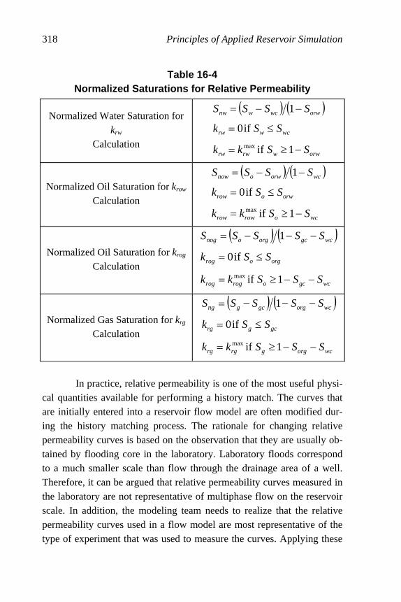
318 Principles of Applied Reservoir Simulation
Table 16-4 Normalized Saturations for Relative Permeability
Normalized Water Saturation for krw
Calculation
( ) ( )
orwwrwrw
wcwrw
orwwcwnw
SSkk
SSk
SSSS
−≥=
≤=
−−=
1if
if0
1
max
Normalized Oil Saturation for krow Calculation
( ) ( )
wcorowrow
orworow
wcorwonow
SSkk
SSk
SSSS
−≥=
≤=
−−=
1if
if0
1
max
Normalized Oil Saturation for krog Calculation
( ) ( )
wcgcorogrog
orgorog
wcgcorgonog
SSSkk
SSk
SSSSS
−−≥=
≤=
−−−=
1if
if0
1
max
Normalized Gas Saturation for krg Calculation
( ) ( )
wcorggrgrg
gcgrg
wcorggcgng
SSSkk
SSk
SSSSS
−−≥=
≤=
−−−=
1if
if0
1
max
In practice, relative permeability is one of the most useful physi-cal quantities available for performing a history match. The curves that are initially entered into a reservoir flow model are often modified dur-ing the history matching process. The rationale for changing relative permeability curves is based on the observation that they are usually ob-tained by flooding core in the laboratory. Laboratory floods correspond to a much smaller scale than flow through the drainage area of a well. Therefore, it can be argued that relative permeability curves measured in the laboratory are not representative of multiphase flow on the reservoir scale. In addition, the modeling team needs to realize that the relative permeability curves used in a flow model are most representative of the type of experiment that was used to measure the curves. Applying these

Fluid Properties 319
curves to another type of displacement mechanism can introduce signifi-cant error.
16.5.2 IFLO Three-Phase Relative Permeability
Three-phase relative permeability should be used when oil, wa-ter, and gas are flowing simultaneously. As a practical matter, three-phase relative permeabilities are difficult to measure and correlations are used instead of direct measurements. IFLO contains a correlation for computing a three-phase oil relative permeability curve using two-phase water-oil and gas-oil relative permeability curves. The three-phase oil relative permeability algorithm in IFLO is based on the assumptions that: 1. The water relative permeability curve (krw) obtained for a water-oil
system depends only on water saturation, and 2. The gas relative permeability curve (krg) obtained for a gas-oil sys-
tem depends only on gas saturation. Given these assumptions, krw and krg for water-oil and gas-oil systems, respectively, are also valid for a water-gas-oil system. The three-phase oil relative permeability kro3 is calculated as
( )rgrwrgrom
rogrw
rom
rowromro kkk
k
kk
k
kkk +−⎟⎟
⎠
⎞⎜⎜⎝
⎛+⎟⎟
⎠
⎞⎜⎜⎝
⎛+=3 (16.7)
where
krow = oil relative permeability for water-oil system,
krog = Oil relative permeability for gas-oil system,
krom = oil relative permeability at zero gas saturation and irreducible water saturation.
Equation (16.7) is based on the work by Stone [1973], and Dietrich and Bondor [1976]. Other models of three-phase relative permeability are discussed by Blunt [1999] and Fanchi [2000]. When the three-phase calculation is activated, the user must be sure the input water-oil and gas-oil relative permeability curves are real-istic. For example, if we write irreducible water saturation as Swr, the
320 Principles of Applied Reservoir Simulation
relative permeability constraint krow (1 - Swr) = krog (So + Sw = 1.0) must be satisfied since Sg = 0 in both cases.
16.5.3 Capillary Pressure Capillary pressure is often included in reservoir simulators to help establish the initial distribution of fluids. Capillary pressure is also used in fractured reservoir flow models for controlling the flow of fluids between the fracture and the rock matrix. The role of capillary pressure in flow model initialization is discussed in more detail in the next chap-ter.
The capillary pressure concept is also used to simplify the han-dling of the phase pressures and potentials in the flow equations. The differences in phase pressures
wocow PPP −= (16.8)
and
ogcgo PPP −= (16.9)
are the capillary pressures for oil-water and gas-oil systems, respectively. Experimentally Pcow and Pcgo have been observed to be functions of wa-ter and gas saturations, respectively. Equations (16.8) and (16.9) are used to replace the phase pressures in fluid flow equations with a single phase pressure.
16.5.4 Capillary Pressure and Transition Zones Capillary pressure data is used for determining initial fluid con-tacts and transition zones. The relationship between capillary pressure and elevation is used to establish the initial transition zone in the reser-voir. The oil-water transition zone, for example, is the zone between water only flow and oil only flow. It represents that part of the reservoir where 100% water saturation grades into oil saturation with irreducible water saturation. Similar transition zones may exist at the interface be-tween any pair of immiscible phases.
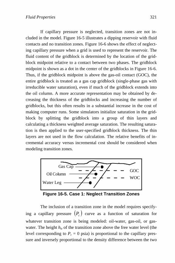
Fluid Properties 321
If capillary pressure is neglected, transition zones are not in-cluded in the model. Figure 16-5 illustrates a dipping reservoir with fluid contacts and no transition zones. Figure 16-6 shows the effect of neglect-ing capillary pressure when a grid is used to represent the reservoir. The fluid content of the gridblock is determined by the location of the grid-block midpoint relative to a contact between two phases. The gridblock midpoint is shown as a dot in the center of the gridblocks in Figure 16-6. Thus, if the gridblock midpoint is above the gas-oil contact (GOC), the entire gridblock is treated as a gas cap gridblock (single-phase gas with irreducible water saturation), even if much of the gridblock extends into the oil column. A more accurate representation may be obtained by de-creasing the thickness of the gridblocks and increasing the number of gridblocks, but this often results in a substantial increase in the cost of making computer runs. Some simulators initialize saturation in the grid-block by splitting the gridblock into a group of thin layers and calculating a thickness weighted average saturation. The resulting satura-tion is then applied to the user-specified gridblock thickness. The thin layers are not used in the flow calculation. The relative benefits of in-cremental accuracy versus incremental cost should be considered when modeling transition zones.
GOC
WOC
Gas Cap
Oil Column
Water Leg
Figure 16-5. Case 1: Neglect Transition Zones
The inclusion of a transition zone in the model requires specify-
ing a capillary pressure ( )cP curve as a function of saturation for
whatever transition zone is being modeled: oil-water, gas-oil, or gas-water. The height htz of the transition zone above the free water level (the level corresponding to Pc = 0 psia) is proportional to the capillary pres-sure and inversely proportional to the density difference between the two

322 Principles of Applied Reservoir Simulation
fluids (see Chapter 3). The height of the transition zone is a function of saturation because capillary pressure depends on saturation. The oil-water transition zone is typically the thickest transition zone because the density difference between oil and water is less than the density differ-ence between gas and an immiscible liquid.
Oil Col.Oil Col.
Gas Cap
Gas Cap
GOC
Water Leg
Oil Col.
WOC
Water Leg
Oil Col.
Figure 16-6. Initial Fluid Distribution in Model without Transition Zone
Figures 16-7 and 16-8 illustrate the initialization of a model con-
taining a nonzero capillary pressure curve. First, the height htz above a specified contact, such as the water-oil contact (WOC), is calculated from Pc and the difference in fluid densities at the contact. The saturation of a gridblock with a midpoint at height htz above the contact is then cal-culated from the relationship between capillary pressure and saturation.
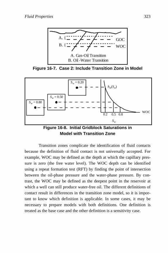
Fluid Properties 323
GOC
WOC
A. {
B. {
A. Gas-Oil TransitionB. Oil -Water Transition
Figure 16-7. Case 2: Include Transition Zone in Model
Sw = 0.80
Sw = 0.50
Sw = 0.20htz(Sw)
0.2 0.5 0.8
Sw
WOC
Figure 16-8. Initial Gridblock Saturations in Model with Transition Zone
Transition zones complicate the identification of fluid contacts because the definition of fluid contact is not universally accepted. For example, WOC may be defined as the depth at which the capillary pres-sure is zero (the free water level). The WOC depth can be identified using a repeat formation test (RFT) by finding the point of intersection between the oil-phase pressure and the water-phase pressure. By con-trast, the WOC may be defined as the deepest point in the reservoir at which a well can still produce water-free oil. The different definitions of contact result in differences in the transition zone model, so it is impor-tant to know which definition is applicable. In some cases, it may be necessary to prepare models with both definitions. One definition is treated as the base case and the other definition is a sensitivity case.

324 Principles of Applied Reservoir Simulation
Exercises Exercise 16.1A Suppose the bubble point pressure is 2400 psia in a res-ervoir with 30% irreducible water saturation. Is the reservoir saturated or undersaturated at an initial reservoir pressure of 2515 psia? Exercise 16.1B List the fluid phases that are present at initial conditions. Exercise 16.2A The pressure at the GOC in a gas reservoir with an oil rim is equal to the bubble point pressure. Suppose gas is produced from the gas cap. Will the resulting pressure at the GOC be above or below the bubble point pressure? Exercise 16.2B Suppose the bubble point pressure of oil in a reservoir simulator gridblock is 2514 psia prior to depletion. If the gridblock pres-sure drops to 2500 psia, will the gridblock contain any free gas? Exercise 16.3 A gas condensate reservoir has a dew point pressure of 2500 psia. If condensate drops out at the rate of 500 STB/psia drawdown below the dew point pressure, how much condensate will drop out if the reservoir pressure declines from 2600 psia to 2300 psia? Exercise 16.4A Using data in the file CS_HM.DAT, calculate the oil formation volume factor in a gridblock that has a pressure of 4014.7 psia. Note: based on the bubble point pressure in the data file, the gridblock is undersaturated. Exercise 16.4B Is there free gas in the gridblock? Exercise 16.4C Run file CS_HM.DAT and report the total initial fluid volumes in place in the reservoir. Do the model results support your an-swer to Part B?

Fluid Properties 325
Exercise 16.5A Using data in the file CS_HM.DAT, calculate oil viscos-ity in a gridblock that has a pressure of 4014.7 psia. Note: based on the bubble point pressure in the data file, the gridblock is undersaturated. Exercise 16.5B Using data in the file CS_HM.DAT, calculate the solu-tion gas-oil ratio in a gridblock that has a pressure of 4014.7 psia. Note: based on the bubble point pressure in the data file, the gridblock is un-dersaturated. Exercise 16.6A Use the real gas law PV ZnRT= to find a general ex-pression for gas formation volume factor Bg. Use subscripts "s" and "r" to denote surface conditions and reservoir conditions, respectively. Exercise 16.6B Calculate Bg using {Ps = 14.7 psia, Ts = 60oF, Zs = 1} and {Pr = 2175 psia, Tr = 140oF, Zr = 0.9}. Express Bg as reservoir cubic feet per standard cubic feet (RCF/SCF). Exercise 16.6C Calculate Bg using {Ps = 1 atm, Ts = 20oC, Zs = 1} and { Pr = 15 MPa, Tr = 60oC, Zr = 0.9}. Express Bg as reservoir cubic meters per standard cubic meter (Rm3/Sm3). Exercise 16.6D What is the difference between the calculation in Part B and the calculation in Part C? Exercise 16.7A Data file EXAM9_PSI models depletion of a gas reser-voir with aquifer support. Initial reservoir pressure is approximately
1947 psia. Run the model at a temperature of 226°F and record time,
pressure, gas rate and water rate at the end of the run. Report the gas vis-cosity in the gas PVT table at 2015 psia pressure.
Exercise 16.7B Repeat Part A at a temperature of 150°F. Exercise 16.7C Explain the differences in model performance. For this example, neglect the temperature dependence of water properties.

326 Principles of Applied Reservoir Simulation
Exercise 16.8A A reservoir gridblock has a length of 1000 ft, a width of 2000 ft, and a gross thickness of 15 ft. What is the bulk volume of the gridblock? Express your answer in ft3, bbl, and m3. Exercise 16.8B If the reservoir gridblock porosity is 0.2 and the net-to-gross ratio is 0.8, what is the pore volume of the gridblock? Express your answer in ft3, bbl, and m3. Exercise 16.8C If the reservoir gridblock has a gas saturation of 0.7, what is the volume of gas in the gridblock? Express your answer in ft3, bbl, and m3.
Exercise 16.9A Calculate the pore volume of a gridblock with ∆x = 200,
∆y = 200 ft, ∆z = 80 ft, φ = 0.20, and net-to-gross ratio = 0.9. Express
your answer in reservoir barrels. Note: 1 bbl = 5.6146 cu ft. Exercise 16.9B If initial oil saturation is 0.7 and residual oil saturation is 0.25, what is the volume of mobile oil in the gridblock? Express your answer in reservoir barrels (RB). Exercise 16.9C If a well produces 500 RB oil/day from the gridblock, how long does it take to produce all of the mobile oil in the gridblock?
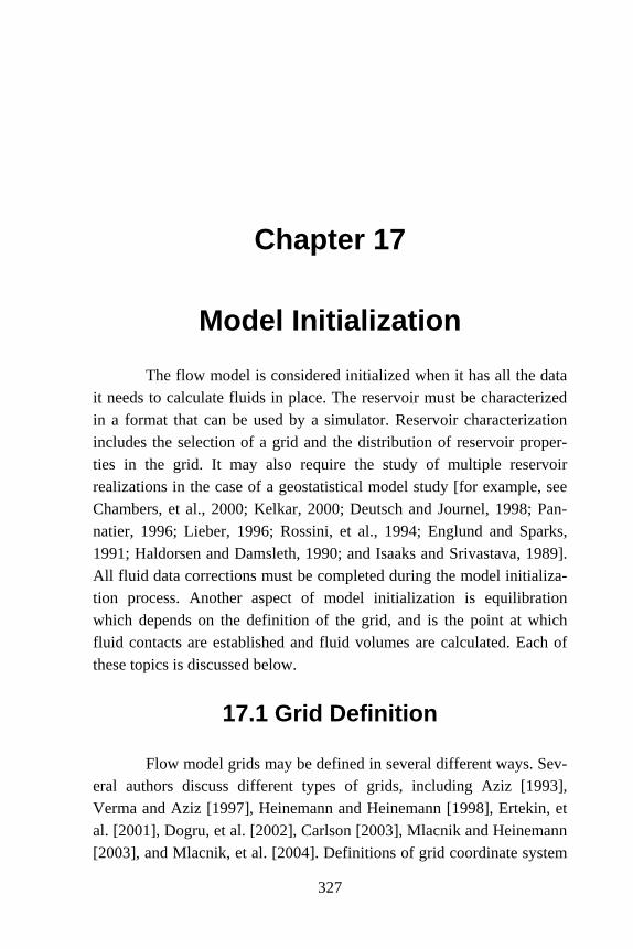
327
Chapter 17
Model Initialization
The flow model is considered initialized when it has all the data it needs to calculate fluids in place. The reservoir must be characterized in a format that can be used by a simulator. Reservoir characterization includes the selection of a grid and the distribution of reservoir proper-ties in the grid. It may also require the study of multiple reservoir realizations in the case of a geostatistical model study [for example, see Chambers, et al., 2000; Kelkar, 2000; Deutsch and Journel, 1998; Pan-natier, 1996; Lieber, 1996; Rossini, et al., 1994; Englund and Sparks, 1991; Haldorsen and Damsleth, 1990; and Isaaks and Srivastava, 1989]. All fluid data corrections must be completed during the model initializa-tion process. Another aspect of model initialization is equilibration which depends on the definition of the grid, and is the point at which fluid contacts are established and fluid volumes are calculated. Each of these topics is discussed below.
17.1 Grid Definition Flow model grids may be defined in several different ways. Sev-eral authors discuss different types of grids, including Aziz [1993], Verma and Aziz [1997], Heinemann and Heinemann [1998], Ertekin, et al. [2001], Dogru, et al. [2002], Carlson [2003], Mlacnik and Heinemann [2003], and Mlacnik, et al. [2004]. Definitions of grid coordinate system
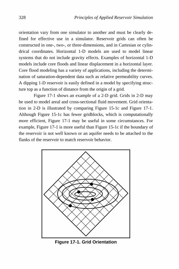
328 Principles of Applied Reservoir Simulation
orientation vary from one simulator to another and must be clearly de-fined for effective use in a simulator. Reservoir grids can often be constructed in one-, two-, or three-dimensions, and in Cartesian or cylin-drical coordinates. Horizontal 1-D models are used to model linear systems that do not include gravity effects. Examples of horizontal 1-D models include core floods and linear displacement in a horizontal layer. Core flood modeling has a variety of applications, including the determi-nation of saturation-dependent data such as relative permeability curves. A dipping 1-D reservoir is easily defined in a model by specifying struc-ture top as a function of distance from the origin of a grid. Figure 17-1 shows an example of a 2-D grid. Grids in 2-D may be used to model areal and cross-sectional fluid movement. Grid orienta-tion in 2-D is illustrated by comparing Figure 15-1c and Figure 17-1. Although Figure 15-1c has fewer gridblocks, which is computationally more efficient, Figure 17-1 may be useful in some circumstances. For example, Figure 17-1 is more useful than Figure 15-1c if the boundary of the reservoir is not well known or an aquifer needs to be attached to the flanks of the reservoir to match reservoir behavior.
Figure 17-1. Grid Orientation

Model Initialization 329
The use of 2-D grids for full field modeling has continued to be popular even as computer power has increased and made large 3-D mod-els practical. Figure 17-2 shows a simple 3-D grid that is often called a “layer cake” grid. Techniques are available for approximating the verti-cal distribution of fluids in 2-D cross-sectional and 3-D models by modifying relative permeability and capillary pressure curves. The modi-fied curves are called pseudo curves. An example of a pseudoization technique is the vertical equilibrium (VE) approximation. The principal VE assumption is that fluid segregation in the vertical dimension is in-stantaneous. This assumption is approximated in nature when vertical flow is rapid relative to horizontal flow. This situation occurs when the vertical permeability of the reservoir is comparable in magnitude to its horizontal permeability, and when density differences are significant, such as in gas-oil or gas-water systems. For more discussion of specific pseudoization techniques, see authors such as Taggart, et al. [1995], Ertekin, et al. [2001], Walsh and Lake [2003], and Carlson [2003] and their references.
j
i
k
Figure 17-2. Example of a 3-D "layer cake" grid One reason for the continuing popularity of 2-D grids is that the expectation of what is appropriate grid resolution has changed as simula-tion technology evolved. Thus, even though 3-D models can be used today with the grid resolution that was considered acceptable a decade ago for 2-D models, modern expectations often require that even finer grids be used for the same types of problems. This is an example of a task expanding to fit the available resources. Increased grid resolution

330 Principles of Applied Reservoir Simulation
does not guarantee better reservoir management decisions. Indeed, it can be argued that the technological ability to add complexity is making it more difficult for people to develop a “big picture” understanding of the system being studied because they are too busy focusing on the details of a complex model. Once again, a judicious use of Ockham’s Razor is ad-visable in selecting a reservoir grid. The grid should be appropriate for achieving study objectives. In many cases, simple conceptual models may be useful in se-lecting a final grid for the model study, especially when determining the number of layers. As an illustration, suppose we want to track flood front movement in a very large field. In this case, we want as much areal defi-nition as possible (at least three to five gridblocks between each gridblock containing a well), but this may mean loss of vertical defini-tion. A way to resolve the problem is to set up one or more cross-section models representing different parts of the field. Vertical conformance effects in these regions are modeled in detail by calculating flow per-formance with the cross-section models. The flow performance of a detailed cross-section model is then matched by adjusting relative per-meability curves in a model with fewer layers. The resulting pseudorelative permeability curves are considered acceptable for use in an areal model.
17.1.1 Non-Cartesian Grids
Near-wellbore coning models may be either 2-D or 3-D grids, but are defined in cylindrical rather than Cartesian coordinates. Coning (or radial) models are designed to study rapid pressure and saturation changes. Figure 17-3 shows an example of a radial grid. High through-put, that is, large flow rate through relatively small, near-wellbore gridblocks is most effectively simulated by a fully implicit formulation. Implicit pressure – explicit saturation (IMPES) can be used to model coning, but timesteps must be very small. Small timesteps are not a prob-lem if the duration of the modeled history is short, as it would be in the case of a pressure transient test.

Model Initialization 331
LGR Radial Grid
Figure 17-3. LGR and Radial Grids
Local grid refinement (LGR) is used to provide additional grid definition in a few selected regions of a larger grid. Raleigh [1991] com-pared LGR with a radial grid (Figure 17-3) and showed that the results are comparable. An LGR grid is an example of a flexible or unstructured grid. A flexible grid is made up of polygons in 2-D (polyhedra in 3-D) whose shape and size vary from one subregion to another in the modeled region. The LGR grid shown in Figure 17-3 is an example of a hybrid grid [Evans, 2004]. Hybrid grids are a combination of two different types of grids. In this case, it is the combination of a radial grid and a Cartesian grid.
Although many grid preparation options are available, improving grid preparation capability is an ongoing research and development topic. For example, some flow simulators are based on control volume finite element formulations that use triangular meshes in 2-D (tetrahedral meshes in 3-D). Finite difference grids typically display global orthogo-nality in which the grid axes are aligned along orthogonal coordinate directions. Examples of globally orthogonal coordinate systems include
the Cartesian x-y-z system and the cylindrical r-θ-z system. Grids with
global orthogonality may be distorted to fit local irregularities such as faults using corner point geometry as described below. By contrast, finite element grids display orthogonality in which gridblock boundaries are perpendicular to lines joining gridblock nodes on opposite sides of each boundary. An example of a locally orthogonal grid is a perpendicular
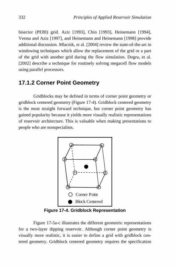
332 Principles of Applied Reservoir Simulation
bisector (PEBI) grid. Aziz [1993], Chin [1993], Heinemann [1994], Verma and Aziz [1997], and Heinemann and Heinemann [1998] provide additional discussion. Mlacnik, et al. [2004] review the state-of-the-art in windowing techniques which allow the replacement of the grid or a part of the grid with another grid during the flow simulation. Dogru, et al. [2002] describe a technique for routinely solving megacell flow models using parallel processors.
17.1.2 Corner Point Geometry
Gridblocks may be defined in terms of corner point geometry or gridblock centered geometry (Figure 17-4). Gridblock centered geometry is the most straight forward technique, but corner point geometry has gained popularity because it yields more visually realistic representations of reservoir architecture. This is valuable when making presentations to people who are nonspecialists.
Corner Point
Block Centered
Figure 17-4. Gridblock Representation
Figure 17-5a-c illustrates the different geometric representations for a two-layer dipping reservoir. Although corner point geometry is visually more realistic, it is easier to define a grid with gridblock cen-tered geometry. Gridblock centered geometry requires the specification

Model Initialization 333
of the lengths of each side of the gridblock and the gridblock center or top. Corner point geometry requires the specification of the location of all eight corners of the gridblock. This is most readily accomplished with a computer program.
••
••
••
••
Figure 17-5a. Conventional Grid with Rectangles
•
••
••
••
•
Figure 17-5b. Dip-aligned Grid with Rectangles
•
•
•
••
••
•
Figure 17-5c. Conventional Grid with Parallelograms
There is little computational difference between the results of corner point and gridblock centered geometry. One caution should be noted with respect to corner point geometry. It is possible to define very
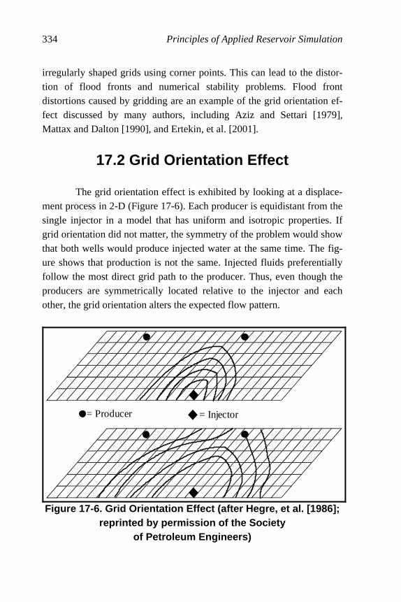
334 Principles of Applied Reservoir Simulation
irregularly shaped grids using corner points. This can lead to the distor-tion of flood fronts and numerical stability problems. Flood front distortions caused by gridding are an example of the grid orientation ef-fect discussed by many authors, including Aziz and Settari [1979], Mattax and Dalton [1990], and Ertekin, et al. [2001].
17.2 Grid Orientation Effect The grid orientation effect is exhibited by looking at a displace-ment process in 2-D (Figure 17-6). Each producer is equidistant from the single injector in a model that has uniform and isotropic properties. If grid orientation did not matter, the symmetry of the problem would show that both wells would produce injected water at the same time. The fig-ure shows that production is not the same. Injected fluids preferentially follow the most direct grid path to the producer. Thus, even though the producers are symmetrically located relative to the injector and each other, the grid orientation alters the expected flow pattern.
= Producer = Injector
Figure 17-6. Grid Orientation Effect (after Hegre, et al. [1986]; reprinted by permission of the Society
of Petroleum Engineers)

Model Initialization 335
Figure 17-6 shows the effect on frontal advance. In this case, the front arrives sooner at the producer in the upper right than the producer in the upper left. If these results are incorporated in a reservoir manage-ment plan, they can reduce its overall effectiveness. Another example of the grid orientation effect arises in connec-tion with the modeling of pattern floods. Figure 17-7 illustrates two grids that can be used to model flow in a five-spot pattern. The parallel grid results in earlier breakthrough of injected fluids than the diagonal grid. This effect can be traced to the finite difference representation of the fluid flow equations.
Y
Y
X
X
ParallelGrid
DiagonalGrid
Figure 17-7. Parallel and Diagonal Grids (after Todd, et al. [1972]; reprinted by permission of the Society
of the Petroleum Engineers)
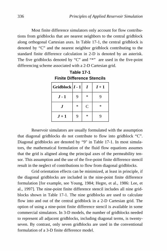
336 Principles of Applied Reservoir Simulation
Most finite difference simulators only account for flow contribu-tions from gridblocks that are nearest neighbors to the central gridblock along orthogonal Cartesian axes. In Table 17-1, the central gridblock is denoted by “C” and the nearest neighbor gridblock contributing to the standard finite difference calculation in 2-D is denoted by an asterisk. The five gridblocks denoted by “C” and “*” are used in the five-point differencing scheme associated with a 2-D Cartesian grid.
Table 17-1 Finite Difference Stencils
Gridblock I - 1 I I + 1
J - 1 9 * 9
J * C *
J + 1 9 * 9
Reservoir simulators are usually formulated with the assumption that diagonal gridblocks do not contribute to flow into gridblock “C”. Diagonal gridblocks are denoted by “9" in Table 17-1. In most simula-tors, the mathematical formulation of the fluid flow equations assumes that the grid is aligned along the principal axes of the permeability ten-sor. This assumption and the use of the five-point finite difference stencil result in the neglect of contributions to flow from diagonal gridblocks.
Grid orientation effects can be minimized, at least in principle, if the diagonal gridblocks are included in the nine-point finite difference formulation [for example, see Young, 1984; Hegre, et al., 1986: Lee, et al., 1997]. The nine-point finite difference stencil includes all nine grid-blocks shown in Table 17-1. The nine gridblocks are used to calculate flow into and out of the central gridblock in a 2-D Cartesian grid. The option of using a nine-point finite difference stencil is available in some commercial simulators. In 3-D models, the number of gridblocks needed to represent all adjacent gridblocks, including diagonal terms, is twenty-seven. By contrast, only seven gridblocks are used in the conventional formulation of a 3-D finite difference model.

Model Initialization 337
17.3 IFLO Initialization Model
An equilibrium initialization algorithm and a gravity segregation algorithm are available as options in IFLO. These options are described below.
17.3.1 Equilibrium Initialization
Suppose a gridblock has a gas-oil contact (GOC) and a water-oil contact (WOC) as shown in Figure 17-8. The pressure at GOC is PGOC. Similarly, PWOC is the pressure at WOC. The initial oil phase pressure assigned to the gridblock in Figure 17-8 is determined by PWOC, PGOC and the depth of the node (midpoint) relative to the respective contact elevations. The equilibrium initialization algorithm is described in detail by Ammer, et al. [1991]. We closely follow their presentation here.
The oil density ROWOC and water density RWWOC at WOC are calculated using the pressure PWOC. The water-oil capillary pressure PCOW is calculated for the gridblock at the midpoint elevation EL using the densities at WOC, thus:
( ) ( )ELWOCRORW144
1PCOW WOCWOC −⋅−= (17.1)
The initial water saturation SWI for the gridblock is calculated at the midpoint elevation using PCOW and the following algorithm:
1. If PCOW ≥ PCOW at irreducible water saturation Swr, set SWI = Swr.
2. If PCOW ≤ PCOW at water saturation Sw = 1, set SWI = 1. 3. If PCOW(Sw = 1) < PCOW < PCOW(Sw = Swr), then interpolate the
value of SWI from the user-input water-oil capillary pressure curve. The notation PCOW(Sw = 1) should be read as the variable PCOW is evaluated at Sw = 1 since PCOW is a function of Sw. Similarly, the nota-tion PCOW(Sw = Swr) says that the variable PCOW is evaluated at Sw = Swr.

338 Principles of Applied Reservoir Simulation
y
x
zE
L (+
) (+)
(+)GOC
WOC
Datum
Figure 17-8. Depths for Initialization Algorithm A similar calculation is performed to determine initial oil phase pressure at the GOC using gas and oil densities. The gas density RGGOC and oil density ROGOC at GOC are calculated using the pressure PGOC. The gas-oil capillary pressure PCGO is calculated for the gridblock at the midpoint elevation EL using the densities at GOC, thus:
( ) ( )ELGOCRGRO144
1PCGO GOCGOC −⋅−= (17.2)
The initial gas saturation (SGI) and initial oil saturation (SOI) for the gridblock are calculated at the midpoint elevation using PCGO, the pre-vious calculation of SWI, and the following algorithm:
a, If PCGO ≤ PCGO at total liquid saturation SL = 1, set SGI = 0.
b. If PCGO ≥ PCGO at SL = Swr, set SGI = 1 - SWI. c. If PCGO(SL = 1) < PCGO < PCGO (SL = Swr), then interpolate
the value of SGI from the user-input water-oil capillary pressure curve.
The notation PCGO(SL = 1) should be read as the variable PCGO is evaluated at SL = 1 since PCGO is a function of SL. Similarly, the nota-tion PCGO(SL = Swr) says that the variable PCOW is evaluated at SL =
Swr. Oil saturation is obtained from the constraint So + Sw + Sg =1.
The initial oil phase pressure P is calculated using the saturations determined above to define the appropriate pressure gradient. The algo-rithm for calculating P follows: Case 1: If SWI = 1, then
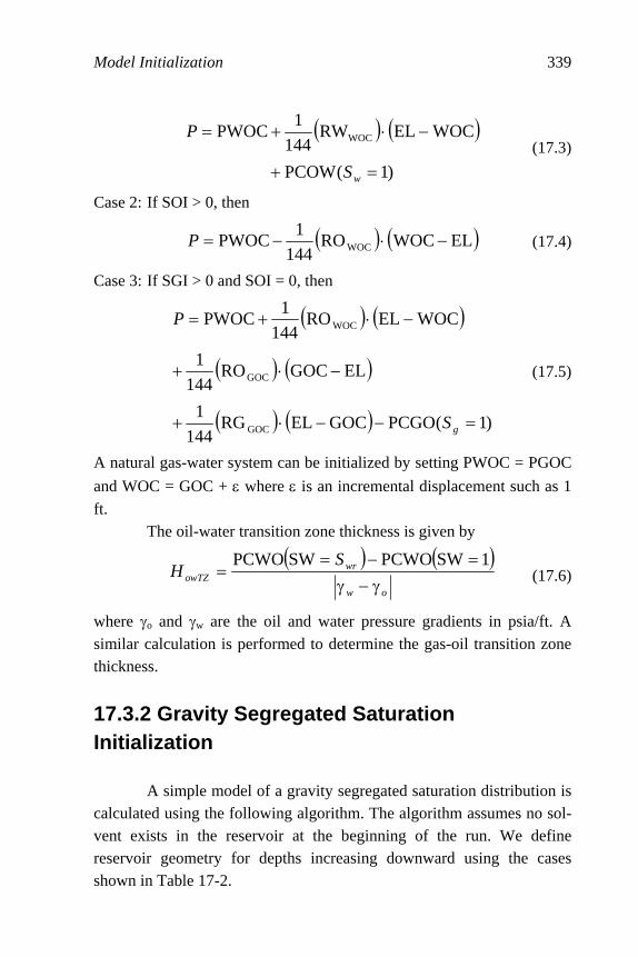
Model Initialization 339
( ) ( )
)1(PCOW
WOCELRW144
1PWOC WOC
=+
−⋅+=
wS
P(17.3)
Case 2: If SOI > 0, then
( ) ( )ELWOCRO144
1PWOC WOC −⋅−=P (17.4)
Case 3: If SGI > 0 and SOI = 0, then
( ) ( )
( ) ( )
( ) ( ) )1(PCGOGOCELRG144
1
ELGOCRO144
1
WOCELRO144
1PWOC
GOC
GOC
WOC
=−−⋅+
−⋅+
−⋅+=
gS
P
(17.5)
A natural gas-water system can be initialized by setting PWOC = PGOC
and WOC = GOC + ε where ε is an incremental displacement such as 1
ft. The oil-water transition zone thickness is given by
( ) ( )
ow
wrowTZ
SH
γ−γ=−=
=1SWPCWOSWPCWO
(17.6)
where γo and γw are the oil and water pressure gradients in psia/ft. A similar calculation is performed to determine the gas-oil transition zone thickness.
17.3.2 Gravity Segregated Saturation Initialization A simple model of a gravity segregated saturation distribution is calculated using the following algorithm. The algorithm assumes no sol-vent exists in the reservoir at the beginning of the run. We define reservoir geometry for depths increasing downward using the cases shown in Table 17-2.
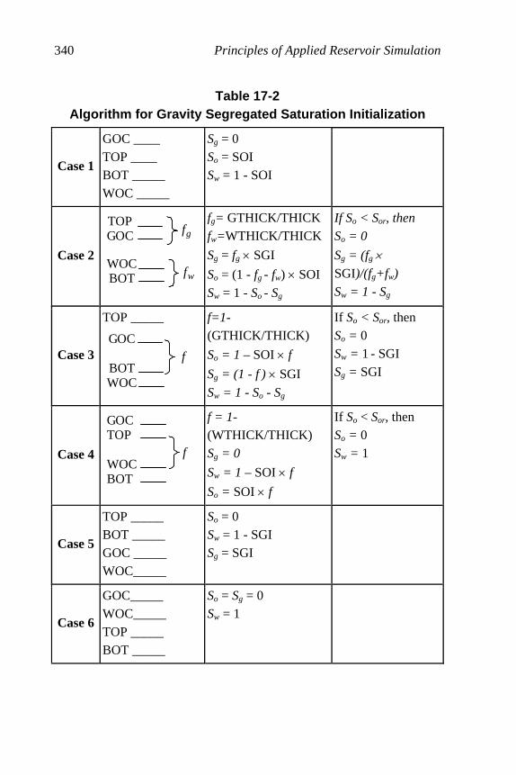
340 Principles of Applied Reservoir Simulation
Table 17-2 Algorithm for Gravity Segregated Saturation Initialization
Case 1
GOC ____ TOP ____ BOT _____ WOC _____
Sg = 0 So = SOI Sw = 1 - SOI
Case 2
TOPGOC fg
WOCBOT fw
fg= GTHICK/THICK fw=WTHICK/THICK
Sg = fg × SGI
So = (1 - fg - fw) × SOI
Sw = 1 - So - Sg
If So < Sor, then
So = 0
Sg = (fg ×
SGI)/(fg+fw)
Sw = 1 - Sg
Case 3
TOP _____
GOC
BOTWOC
f
f=1-
(GTHICK/THICK)
So = 1 – SOI × f
Sg = (1 - f ) × SGI
Sw = 1 - So - Sg
If So < Sor, then So = 0
Sw = 1 - SGI Sg = SGI
Case 4
GOCTOP
WOCBOT
f
f = 1-
(WTHICK/THICK) Sg = 0
Sw = 1 – SOI × f
So = SOI × f
If So < Sor, then So = 0
Sw = 1
Case 5
TOP _____ BOT _____ GOC _____ WOC_____
So = 0 Sw = 1 - SGI Sg = SGI
Case 6
GOC_____ WOC_____ TOP _____ BOT _____
So = Sg = 0 Sw = 1

Model Initialization 341
Gridblock elevations and thicknesses are calculated using the re-lationships
Gridblock BOT = EL + 0.5 *DZ
Gridblock THICK = DZ
Gridblock TOP = BOT - THICK
Water zone thickness
WTHICK = BOT - WOC
Gas zone thickness
GTHICK = GOC - TOP
The user must specify the initial oil saturation (SOI) for an oil-water sys-tem and the initial gas saturation (SGI) for a water-gas system. Given the initial saturations SOI and SGI, the algorithm in Table 17-2 is applied. Water saturation is calculated as Sw = 1 - So - Sg in all cases. Cases 2 through 4 require the user to enter residual oil saturation Sor.
17.4 Case Study: Introduction We introduce a case study in this chapter that is designed to in-crease your understanding of the reservoir simulation process, and to give you experience applying a simulator to a realistic model study. The case study is introduced in this chapter, and continued in Chapters 18 and 19.
17.4.1 Reservoir Management Objective
The first step in a study is to identify its objectives. The reservoir management objective of this case study is to optimize production from a dipping, undersaturated oil reservoir. Constraints imposed on the case study objective are presented after we review some background informa-tion about the field of interest. The background information should be sufficient to initialize the flow model.
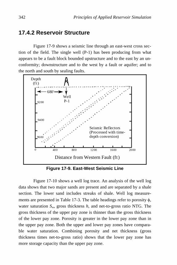
342 Principles of Applied Reservoir Simulation
17.4.2 Reservoir Structure Figure 17-9 shows a seismic line through an east-west cross sec-tion of the field. The single well (P-1) has been producing from what appears to be a fault block bounded upstructure and to the east by an un-conformity; downstructure and to the west by a fault or aquifer; and to the north and south by sealing faults.
680'WellP-1
Seismic Reflectors(Processed with time-depth conversion)
Distance from Western Fault (ft )
9200
9400
9600
1600 20001200400 8000
Depth(f t )
Figure 17-9. East-West Seismic Line
Figure 17-10 shows a well log trace. An analysis of the well log
data shows that two major sands are present and are separated by a shale section. The lower sand includes streaks of shale. Well log measure-
ments are presented in Table 17-3. The table headings refer to porosity φ, water saturation Sw, gross thickness h, and net-to-gross ratio NTG. The gross thickness of the upper pay zone is thinner than the gross thickness of the lower pay zone. Porosity is greater in the lower pay zone than in the upper pay zone. Both the upper and lower pay zones have compara-ble water saturation. Combining porosity and net thickness (gross thickness times net-to-gross ratio) shows that the lower pay zone has more storage capacity than the upper pay zone.
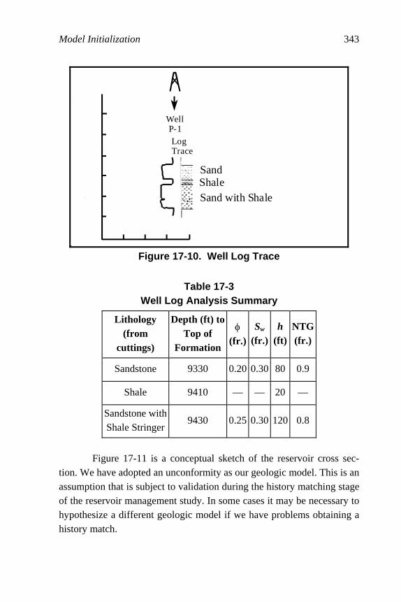
Model Initialization 343
SandShaleSand with Shale
LogTrace
WellP-1
Figure 17-10. Well Log Trace
Table 17-3 Well Log Analysis Summary
Lithology (from
cuttings)
Depth (ft) to Top of
Formation
φ (fr.)
Sw (fr.)
h (ft)
NTG(fr.)
Sandstone 9330 0.20 0.30 80 0.9
Shale 9410 — — 20 —
Sandstone withShale Stringer
9430 0.25 0.30 120 0.8
Figure 17-11 is a conceptual sketch of the reservoir cross sec-tion. We have adopted an unconformity as our geologic model. This is an assumption that is subject to validation during the history matching stage of the reservoir management study. In some cases it may be necessary to hypothesize a different geologic model if we have problems obtaining a history match.

344 Principles of Applied Reservoir Simulation
Oil
Water
ImpermeableCap Rock
Figure 17-11. Conceptual Sketch of Reservoir Cross Section
(after Clark [1969]; reprinted by permission of the Society of Petroleum Engineers)
17.4.3 Drill Stem Test Well P-1 logs and cores show the presence of two major sands. A drill stem test (DST) run in both major sands yielded the information summarized in Table 17-4.
Table 17-4 Summary of Well P-1 DST Results
Wellbore Radius 0.25 ft
Wellbore Skin -0.5
Initial Pressure 3936 psia at 9360 ft
No-Flow Boundary Within 700 ft
Permeability is estimated from the DST data for both sands. Ta-ble 17-5 presents the results, together with average water saturation (Sw) values and oil saturation (So) values, for both major sands.
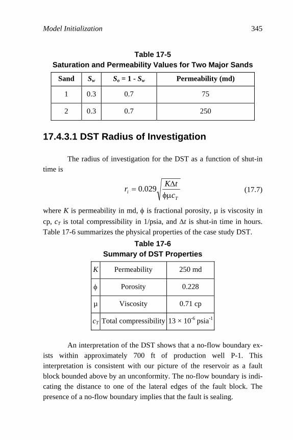
Model Initialization 345
Table 17-5 Saturation and Permeability Values for Two Major Sands
Sand Sw So = 1 - Sw Permeability (md)
1 0.3 0.7 75
2 0.3 0.7 250
17.4.3.1 DST Radius of Investigation
The radius of investigation for the DST as a function of shut-in time is
T
i c
tKr
φµ∆
= 029.0 (17.7)
where K is permeability in md, φ is fractional porosity, µ is viscosity in
cp, cT is total compressibility in 1/psia, and ∆t is shut-in time in hours. Table 17-6 summarizes the physical properties of the case study DST.
Table 17-6 Summary of DST Properties
K Permeability 250 md
φ Porosity 0.228
µ Viscosity 0.71 cp
cT Total compressibility 13 × 10-6 psia-1
An interpretation of the DST shows that a no-flow boundary ex-
ists within approximately 700 ft of production well P-1. This interpretation is consistent with our picture of the reservoir as a fault block bounded above by an unconformity. The no-flow boundary is indi-cating the distance to one of the lateral edges of the fault block. The presence of a no-flow boundary implies that the fault is sealing.
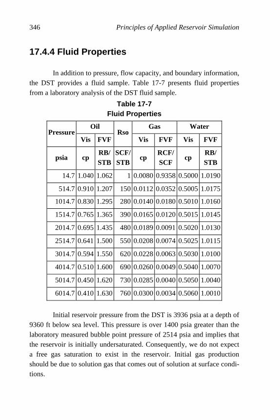
346 Principles of Applied Reservoir Simulation
17.4.4 Fluid Properties In addition to pressure, flow capacity, and boundary information, the DST provides a fluid sample. Table 17-7 presents fluid properties from a laboratory analysis of the DST fluid sample.
Table 17-7 Fluid Properties
Oil Gas Water Pressure
Vis FVFRso
Vis FVF Vis FVF
psia cp RB/STB
SCF/STB
cp RCF/SCF
cp RB/ STB
14.7 1.040 1.062 1 0.0080 0.9358 0.5000 1.0190
514.7 0.910 1.207 150 0.0112 0.0352 0.5005 1.0175
1014.7 0.830 1.295 280 0.0140 0.0180 0.5010 1.0160
1514.7 0.765 1.365 390 0.0165 0.0120 0.5015 1.0145
2014.7 0.695 1.435 480 0.0189 0.0091 0.5020 1.0130
2514.7 0.641 1.500 550 0.0208 0.0074 0.5025 1.0115
3014.7 0.594 1.550 620 0.0228 0.0063 0.5030 1.0100
4014.7 0.510 1.600 690 0.0260 0.0049 0.5040 1.0070
5014.7 0.450 1.620 730 0.0285 0.0040 0.5050 1.0040
6014.7 0.410 1.630 760 0.0300 0.0034 0.5060 1.0010
Initial reservoir pressure from the DST is 3936 psia at a depth of 9360 ft below sea level. This pressure is over 1400 psia greater than the laboratory measured bubble point pressure of 2514 psia and implies that the reservoir is initially undersaturated. Consequently, we do not expect a free gas saturation to exist in the reservoir. Initial gas production should be due to solution gas that comes out of solution at surface condi-tions.
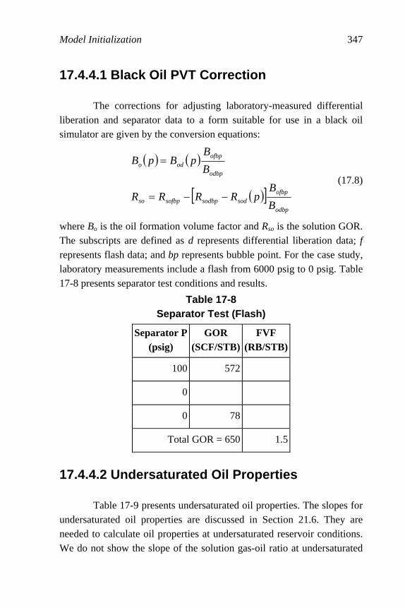
Model Initialization 347
17.4.4.1 Black Oil PVT Correction The corrections for adjusting laboratory-measured differential liberation and separator data to a form suitable for use in a black oil simulator are given by the conversion equations:
( ) ( )
( )[ ]odbp
ofbpsodsodbpsofbpso
odbp
ofbpodo
B
BpRRRR
B
BpBpB
−−=
=
(17.8)
where Bo is the oil formation volume factor and Rso is the solution GOR. The subscripts are defined as d represents differential liberation data; f represents flash data; and bp represents bubble point. For the case study, laboratory measurements include a flash from 6000 psig to 0 psig. Table 17-8 presents separator test conditions and results.
Table 17-8 Separator Test (Flash)
Separator P(psig)
GOR (SCF/STB)
FVF (RB/STB)
100 572
0
0 78
Total GOR = 650 1.5
17.4.4.2 Undersaturated Oil Properties Table 17-9 presents undersaturated oil properties. The slopes for undersaturated oil properties are discussed in Section 21.6. They are needed to calculate oil properties at undersaturated reservoir conditions. We do not show the slope of the solution gas-oil ratio at undersaturated
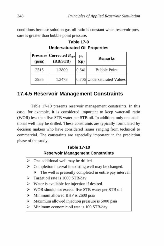
348 Principles of Applied Reservoir Simulation
conditions because solution gas-oil ratio is constant when reservoir pres-sure is greater than bubble point pressure.
Table 17-9 Undersaturated Oil Properties
Pressure(psia)
Corrected Bopb
(RB/STB) µo
(cp)Remarks
2515 1.3800 0.641 Bubble Point
3935 1.3473 0.706 Undersaturated Values
17.4.5 Reservoir Mana gement Constraints
Table 17-10 presents reservoir management constraints. In this case, for example, it is considered important to keep water-oil ratio (WOR) less than five STB water per STB oil. In addition, only one addi-tional well may be drilled. These constraints are typically formulated by decision makers who have considered issues ranging from technical to commercial. The constraints are especially important in the prediction phase of the study.
Table 17-10 Reservoir Management Constraints
Ü One additional well may be drilled. Ü Completion interval in existing well may be changed.
Ü The well is presently completed in entire pay interval.Ü Target oil rate is 1000 STB/day Ü Water is available for injection if desired. Ü WOR should not exceed five STB water per STB oil Ü Minimum allowed BHP is 2600 psia Ü Maximum allowed injection pressure is 5000 psia Ü Minimum economic oil rate is 100 STB/day
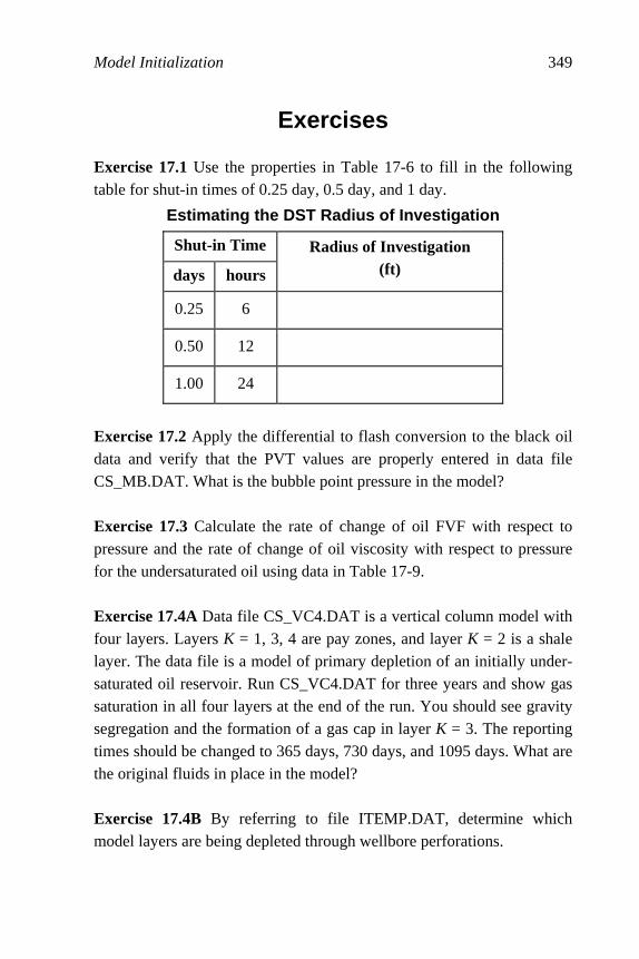
Model Initialization 349
Exercises Exercise 17.1 Use the properties in Table 17-6 to fill in the following table for shut-in times of 0.25 day, 0.5 day, and 1 day.
Estimating the DST Radius of Investigation
Shut-in Time
days hours
Radius of Investigation (ft)
0.25 6
0.50 12
1.00 24
Exercise 17.2 Apply the differential to flash conversion to the black oil data and verify that the PVT values are properly entered in data file CS_MB.DAT. What is the bubble point pressure in the model? Exercise 17.3 Calculate the rate of change of oil FVF with respect to pressure and the rate of change of oil viscosity with respect to pressure for the undersaturated oil using data in Table 17-9. Exercise 17.4A Data file CS_VC4.DAT is a vertical column model with four layers. Layers K = 1, 3, 4 are pay zones, and layer K = 2 is a shale layer. The data file is a model of primary depletion of an initially under-saturated oil reservoir. Run CS_VC4.DAT for three years and show gas saturation in all four layers at the end of the run. You should see gravity segregation and the formation of a gas cap in layer K = 3. The reporting times should be changed to 365 days, 730 days, and 1095 days. What are the original fluids in place in the model? Exercise 17.4B By referring to file ITEMP.DAT, determine which model layers are being depleted through wellbore perforations.
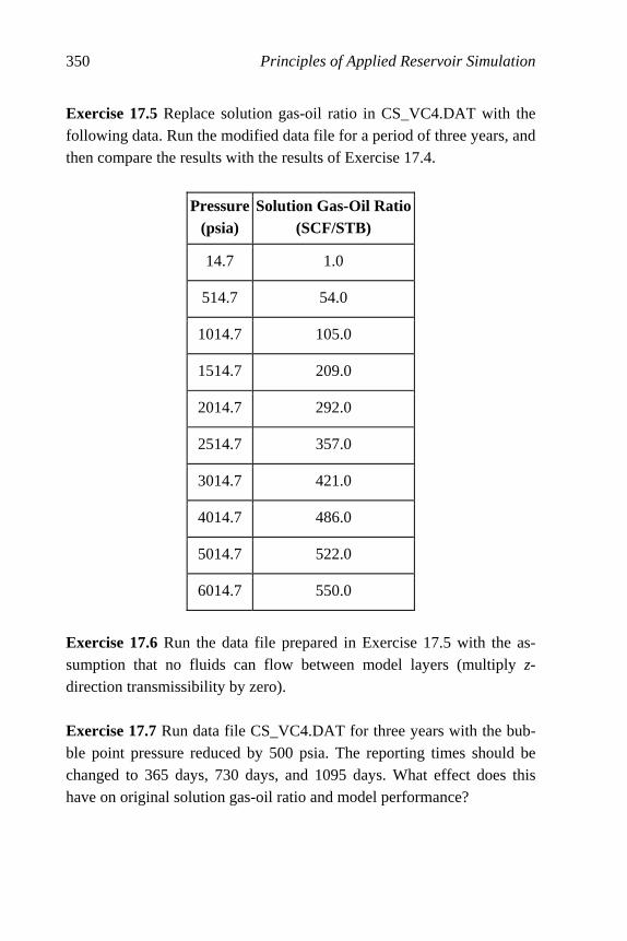
350 Principles of Applied Reservoir Simulation
Exercise 17.5 Replace solution gas-oil ratio in CS_VC4.DAT with the following data. Run the modified data file for a period of three years, and then compare the results with the results of Exercise 17.4.
Pressure(psia)
Solution Gas-Oil Ratio(SCF/STB)
14.7 1.0
514.7 54.0
1014.7 105.0
1514.7 209.0
2014.7 292.0
2514.7 357.0
3014.7 421.0
4014.7 486.0
5014.7 522.0
6014.7 550.0
Exercise 17.6 Run the data file prepared in Exercise 17.5 with the as-sumption that no fluids can flow between model layers (multiply z-
direction transmissibility by zero). Exercise 17.7 Run data file CS_VC4.DAT for three years with the bub-ble point pressure reduced by 500 psia. The reporting times should be changed to 365 days, 730 days, and 1095 days. What effect does this have on original solution gas-oil ratio and model performance?

351
Chapter 18
History Matching Project objectives help define the level of detail that will be in-corporated in a reservoir flow model. Once objectives are defined, it is helpful to think of the study proceeding in three stages: the history matching stage; a calibration stage, which provides a smooth transition between the first and third stages; and the prediction stage. The first step of the history matching stage is the collection and analysis of data.
18.1 Data Preparation Data must be acquired and evaluated with a focus on its quality and the identification of relevant drive mechanisms that should be in-cluded in the model [for example, see Crichlow, 1977; Saleri, et al., 1992; Raza, 1992; Carlson, 2003]. Given that information, it is possible to select the type of model that will be needed for the study: conceptual, window area, or full field model. In many cases all three of these model types may be required, as Fanchi, et al. [1996] have illustrated. Data must be acquired for each model. Some of the data that is required for a model study can be found in existing reports. The modeling team should find as many reports as it can from as many disciplines as possible. Table 18-1 lists the types of data that are needed in a model study. A review of geophysical, geologi-cal, petrophysical, and engineering reports provides a background on

352 Principles of Applied Reservoir Simulation
how the project has been developed and what preconceived interpreta-tions have been established. During the course of the study, it may be necessary to develop not only a new view of the reservoir, but also to prepare an explanation of why the new view is superior to a previously approved interpretation. If significant gaps exist in the reports, particu-larly regarding the historical performance of the field, it is wise to update them.
Table 18-1 Data Required for a Simulation Study
Property Sources
Permeability Pressure transient testing, Core analyses, Correlations, Well per-formance
Porosity, Rock compressibility
Core analyses, Well logs
Relative permeability and capillary pressure
Laboratory core flow tests
Saturations Well logs, Core analyses, Pressure cores, Single well tracer tests
Fluid property (PVT) data Laboratory analyses of reservoir fluid samples
Faults, boundaries, fluid con-tacts
Seismic, Pressure transient testing
Aquifers Seismic, Material balance calculations, Regional exploration studies
Fracture spacing, orientation, connectivity
Core analyses, Well logs, Seismic, Pres-sure transient tests, Interference testing, Wellbore performance
Rate and pressure data, com-pletion and workover data
Field performance history

History Matching 353
The pressure range associated with fluid property data should cover the entire range of pressures expected to be encountered over the life of the field. The data should be smooth to enhance computational efficiency and to ensure data consistency. A check on data consistency is a calculation of fluid compressibility. If negative compressibility is en-countered, the data should be corrected. The problem of negative compressibility occurs most often when data is extrapolated beyond measured pressure ranges. Flow units should be determined by reviewing geological and petrophysical data. It is possible to represent the behavior of a flow unit by defining a set of PVT and Rock property tables for each flow unit. PVT property tables contain data that describe fluid properties, while Rock property tables represent relative permeability and capillary pres-sure effects. Each set of PVT or Rock property tables applies to a particular region of gridblocks, hence the collection of gridblocks to which a particular set of PVT or Rock property tables applies is referred to as a PVT or Rock region. The number of flow units, and the corre-sponding number of PVT and Rock regions, should be kept to the minimum needed to achieve the objectives of the study. One of the essential tasks of the data acquisition stage is deter-mining the history of field performance and select data that should be matched during the history matching process. For example, if a gas-water reservoir is being modeled, gas rate is usually specified and water production is matched. By contrast, if an oil reservoir is being modeled, oil rate is specified and water and gas production are matched.
A review of available data may identify gaps or errors in the data. If it does, additional data should be obtained when possible. This may require special laboratory tests, depending on the objectives of the study. If additional field tests are needed, they should be requested and incorporated into the study schedule. Due to project costs and operating constraints, it may be difficult to justify the expense of acquiring more data or delaying the study while additional data is obtained. If measured data cannot be obtained during the scope of the study, then correlations or data from analogous fields will have to be used. Values must be en-tered into the simulator, and it is necessary to select values that can be

354 Principles of Applied Reservoir Simulation
justified. The modeling team should take care to avoid underestimating the amount of work that may be needed to prepare an input data set. It can take as long to collect and prepare the data as it does to do the study.
18.2 Illustrative History Matching Strategies
There is no single, universally accepted strategy for performing a history match. Several authors have presented history matching guide-lines, including Crichlow [1977], Thomas [1982], Mattax and Dalton [1990], Saleri, et al. [1992], and Carlson [2003]. Carlson [2003] pointed out that the guidelines suggested by two or more authors may actually contradict each other. Nevertheless, there are some general guidelines that can help move a history match toward successful completion. Table 18-2 presents one set of history matching guidelines. The first two steps in the table take precedence over the last two steps. If the first two steps cannot be achieved, there is a good chance that the model is inadequate and revisions will be necessary. An inadequate model may be due to a variety of problems: for example, the wrong model was selected, the res-ervoir is poorly characterized, or field data is inaccurate or incomplete. Among the data variables matched in a typical black oil or gas study are pressure, production rate, water-oil ratio (WOR), gas-oil-ratio (GOR), and tracer data if it is available. More specialized studies, such as compositional or thermal studies, should also match data unique to the process, such as well stream composition or the temperature of produced fluids.
The pressure is usually the first dynamic variable to be matched during the history matching process. A comparison of estimated reser-voir pressures obtained from well tests of a single well on successive days shows that errors in reported historical pressures can be up to 10 percent of pressure drawdown. This error may be larger than Peaceman’s correction. As a first approximation, it is sufficient to compare uncor-rected historical pressures directly with model pressures, particularly if your initial interest is in pressure trends and not in actual pressure values.
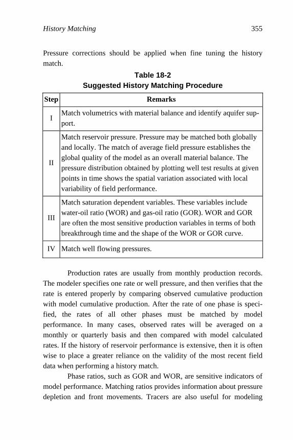
History Matching 355
Pressure corrections should be applied when fine tuning the history match.
Table 18-2 Suggested History Matching Procedure
Step Remarks
I Match volumetrics with material balance and identify aquifer sup-port.
II
Match reservoir pressure. Pressure may be matched both globally and locally. The match of average field pressure establishes the global quality of the model as an overall material balance. The pressure distribution obtained by plotting well test results at given points in time shows the spatial variation associated with local variability of field performance.
III
Match saturation dependent variables. These variables include water-oil ratio (WOR) and gas-oil ratio (GOR). WOR and GOR are often the most sensitive production variables in terms of both breakthrough time and the shape of the WOR or GOR curve.
IV Match well flowing pressures.
Production rates are usually from monthly production records. The modeler specifies one rate or well pressure, and then verifies that the rate is entered properly by comparing observed cumulative production with model cumulative production. After the rate of one phase is speci-fied, the rates of all other phases must be matched by model performance. In many cases, observed rates will be averaged on a monthly or quarterly basis and then compared with model calculated rates. If the history of reservoir performance is extensive, then it is often wise to place a greater reliance on the validity of the most recent field data when performing a history match. Phase ratios, such as GOR and WOR, are sensitive indicators of model performance. Matching ratios provides information about pressure depletion and front movements. Tracers are also useful for modeling
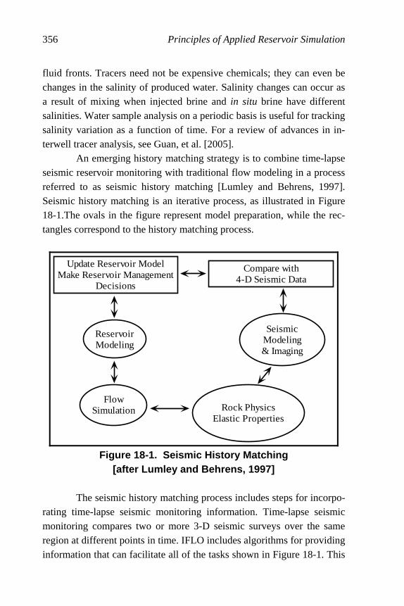
356 Principles of Applied Reservoir Simulation
fluid fronts. Tracers need not be expensive chemicals; they can even be changes in the salinity of produced water. Salinity changes can occur as a result of mixing when injected brine and in situ brine have different salinities. Water sample analysis on a periodic basis is useful for tracking salinity variation as a function of time. For a review of advances in in-terwell tracer analysis, see Guan, et al. [2005].
An emerging history matching strategy is to combine time-lapse seismic reservoir monitoring with traditional flow modeling in a process referred to as seismic history matching [Lumley and Behrens, 1997]. Seismic history matching is an iterative process, as illustrated in Figure 18-1.The ovals in the figure represent model preparation, while the rec-tangles correspond to the history matching process.
Update Reservoir ModelMake Reservoir Management
Decisions
Compare with4-D Seismic Data
ReservoirModeling
SeismicModeling& Imaging
FlowSimulation Rock Physics
Elastic Properties
Figure 18-1. Seismic History Matching
[after Lumley and Behrens, 1997] The seismic history matching process includes steps for incorpo-rating time-lapse seismic monitoring information. Time-lapse seismic monitoring compares two or more 3-D seismic surveys over the same region at different points in time. IFLO includes algorithms for providing information that can facilitate all of the tasks shown in Figure 18-1. This
History Matching 357
has been made possible by the inclusion of a petrophysical model in the flow simulator.
18.3 Key History Matching Parameters A fundamental concept in history matching is the hierarchy of
uncertainty which is a ranking of model input data quality. The modeler uses the hierarchy of uncertainty to rank data from most reliable to least reliable. Changes to model input data are then constrained by the princi-ple that the least reliable data should be changed first. The question is: which data are least reliable? Data reliability is determined when data are collected and evalu-ated for completeness and validity. This is such an important step in establishing a feel for the data that the modeler should be closely in-volved with the review of data. Relative permeability data are typically placed at the top of the hierarchy of uncertainty because they are modi-fied more often than other data. Relative permeability curves are often determined from core floods. As a consequence, the applicability of the final set of curves to the rest of the modeled region is always in doubt. Initial fluid volumes may be modified by changing a variety of input parameters, including relative permeability endpoints and fluid contacts. Model calculated, original fluid volumes in place are con-strained by independent techniques like volumetrics and material balance studies. Attempts to match well data may require changing the producing interval or the productivity index (PI) of a perforation interval. If it is difficult to match well performance in a zone or set of zones, the modeler needs to look at a variety of possibilities, including unexpected comple-tion and wellbore problems. In one study, for example, an unexpectedly high GOR from a perforation interval that was known to be below the gas-oil contact was due to gas flow in the annulus between the tubing and the casing. This result was confirmed by running a cement bond log and finding a leak in the wellbore interval adjacent to the gas cap. Gas cap gas was entering the wellbore and causing greater than expected

358 Principles of Applied Reservoir Simulation
production GOR. This effect can be modeled by a variety of options, depending on the degree of accuracy desired: for example, it could be modeled by altering productivity index (PI) in the well model or by de-signing a near wellbore conceptual model and preparing pseudorelative permeability curves. The choice of method will influence the predictive capability of the model. Thus, a pseudorelative permeability model will allow for high GOR even if the well is recompleted, whereas the PI could be readily corrected at the time of well recompletion to reflect the improvement in wellbore integrity. Map adjustments may also be necessary. This used to be consid-ered a last resort change because map changes required substantial effort to digitize the modified maps and prepare a revised grid. Preprocessing packages and computer-aided geologic modeling are making map changes a more acceptable history match method. In the case of geosta-tistics, a history matching process may actually involve the use of several different geologic models. Each geologic model is called a stochastic image or realization. Toronyi and Saleri [1988] present a detailed discussion of their approach to history matching. It is noteworthy because they provide guidance on how changes in some history match parameters affect matches of saturation and pressure gradients. A summary is presented in Table 18-3 which shows, for example, that a change in pore volume can affect pressure as it changes with time. As another example, relative permeability changes are useful for matching saturation variations in time and space. Notice that fluid property data are seldom changed to match field history. This is because fluid property data tend to be more accurately measured than other model input data.
History matching must not be achieved by making incorrect pa-rameter modifications. For example, matching pressure may be achieved by adjusting rock compressibility, yet the final match value should be within the set of values typically associated with the type of rock in the formation. In general, modified parameter values must be physically meaningful.

History Matching 359
Table 18-3 Influence of Key History Matching Parameters
Parameter Pressure Match Saturation
Match
Pore volume ∆P versus ∆t *
Permeability thickness ∆P versus ∆x ∆S versus ∆x
Relative permeability Not used ∆S versus ∆x and ∆S versus ∆t
Rock compressibility * Not used
Bubble point pressure∆P versus ∆t * *
*Avoid changing if possible
18.4 Evaluating the History Match One way to evaluate the history match is to compare observed and calculated parameters. Typically, observed and calculated parame-ters are compared by making plots of pressure versus time, cumulative production (or injection) versus time, production (or injection) rates ver-sus time, and GOR, WOR, or water cut versus time. Other comparisons can and should be made if data are available. They include, for example, model saturations versus well log saturations, and tracer concentration (such as salinity) versus time. In the case of compositional simulation, dominant components (typically methane) should be plotted as a func-tion of time. In many studies, the most sensitive indicators of model perform-ance are plots of GOR, WOR, or water cut versus time. These plots can be used to identify problem areas. For example, suppose we plot all high and low WOR and GOR wells or plot all high and low pressure wells. A review of such plots may reveal a grouping of wells with the same prob-lem. This can identify the presence of a systematic error or flaw in the
360 Principles of Applied Reservoir Simulation
model that needs to be corrected. If the distribution is random, then local variations in performance due to heterogeneity should be considered.
18.4.1 Deciding on a Match There are several ways to decide if a match is satisfactory. In all cases, a clear understanding of the study objectives should be the stan-dard for making the decision. If a coarse study is being performed, the quality of the match between observed and calculated parameters does not need to be as accurate as it would need to be for a more detailed study. For example, pressure may be considered matched if the differ-ence between calculated and observed pressures is within ±10% drawdown. The tolerance of ±10% is determined by estimating the un-certainty associated with measured field pressures and the required quality of the study. A study demanding greater reliability in predictions may need to reduce the tolerance to ± 5% or even less, but it is unrealis-tic to seek a tolerance of less than 1%. The uncertainty applies not to individual well gauge pressures, which may be measured to a precision of less than one percent, but to estimates of average field or region pres-sure from two or more well tests. The latter error is generally much larger than that of a single well test. In any event, model calculated pres-sure trends should match field or region pressure performance. Another sensitive indicator of the quality of a history match is the match of WOR, GOR, or water cut. Three factors need to be consid-ered: breakthrough time, the magnitude of the difference between observed and calculated values, and trends. Adjustments in the model should be made to improve the quality of each factor. Saleri [1993] has observed that a match of the field is more easily obtained than a match of individual well performance. Indeed, he notes that matching every well is virtually impossible. As a rule of thumb, the field match may be valid for a year or more without updating, and we can expect the well match to be valid for up to six months without updating. Deviations from this rule will vary widely, and will depend on the type of system modeled and the alignment of the interpreted model with reality. Indeed, gas reservoirs

History Matching 361
without aquifer influx may be accurately modeled for the life of the field, while a gas reservoir with complex lithology and water influx may never be satisfactorily matched. Modelers must resist succumbing to the “one more run” syn-drome. This occurs when a modeler (or member of the study team) wants to see “just one more run” to try an idea that has not yet been tried. In practice, a final match is often declared when the time or money allotted for the study is depleted.
18.4.2 Test of Reasonableness
A model may be considered reasonable if it does not violate any known physical constraints. In many cases, a model may be acceptable if it is reasonable. In other situations, not only must physical constraints be satisfied, but approved processes for evaluating data must also be fol-lowed. Thus a model may be reasonable, but if it is based on an innovative technique that is reasonable but not approved, the model will be unacceptable. The modeler may use a method that is in the literature, but the commissioner of the study may have a philosophical or empirical objection to the method. Window area or sector modeling is a good ex-ample of a method that may be reasonable but not acceptable because failure to describe flux across model boundaries adequately can yield poor results. Similarly, the modeler needs to be aware that some model-ing methods are not universally accepted. At the very least, alternative methods may be needed to corroborate the disputed method as part of a sensitivity analysis or model validation exercise.
18.4.3 History Match Limitations History matching (or model calibration) may be thought of as an inverse problem. An inverse problem exists when the dependent variable is the best known aspect of a system and the independent variable must be determined [Oreskes, et al., 1994]. For example, the “dependent vari-able” in oil and gas production is the production performance of the

362 Principles of Applied Reservoir Simulation
field. Production performance depends on input variables such as perme-ability distribution and fluid properties. The goal of the history match is to find a set of input variables that can reconstruct field performance. In the context of an inverse problem, the history matching prob-lem is solved by finding a set of reasonable reservoir parameters that minimizes the difference between model performance and the historical performance of the field. As usual, we must remember that we are solv-ing a nonunique problem whose solution is often as much art as science. The uniqueness problem arises from many factors. Most notable of these are unreliable or limited field data, interpretation errors, and numerical effects. Advances in hardware and software technology have made it possible to minimize the effects of numerical problems, or at least esti-mate their influence on the final history match solution. Data limitations are more difficult to resolve because the system is inherently underde-termined: we do not have enough data to be sure that our final solution is correct. In many instances, observed data can be inaccurate. Kabir and Young [2004] present a case study that discusses how they handled pro-duction data uncertainty. The goal of history matching is to prepare a flow model that can contribute to reservoir management decision making. The modeling team needs to avoid the mistake of preparing a history matched model “at all costs.” The modeling team should pay attention to data from all sources, and use the level of complexity that is needed to satisfy reservoir man-agement objectives.
18.5 Case Study: Data Analysis and Grid Preparation
This section presents more data from the case study introduced in Chapter 17 and subjects that data to reservoir engineering analysis. The analysis includes a geologic estimate of volumetrics and a material balance determination of initial fluids in place. A geologic interpretation guides the preparation of a reservoir grid.

History Matching 363
18.5.1 Production History Well P-1 has produced for a year. Tables 18-4 and 18-5 show its production history. The historical data in Tables 18-4 and 18-5, espe-cially rates, show some variability. The GOR is relatively constant. This implies that the reservoir is undersaturated; that is, reservoir pressure is above bubble point pressure and there is no free gas phase initially. Only one hydrocarbon phase – the liquid phase – is produced at reservoir con-ditions from an undersaturated reservoir. The fact that GOR has not changed significantly over the life of the field is interpreted to mean that the reservoir was undersaturated at initial conditions and is still under-saturated after one year of production.
Table 18-4 Production Rate History
RATES TIME
OIL GAS WATERGOR WOR
Days STB/day MSCF/day STB/day SCF/STB
1 506 227 0 449 0
91 508 228 1 450 0
183 493 229 2 465 0
274 504 228 3 452 0
365 494 226 5 458 0
A review of the water production rate in Table 18-4 shows that there is no initial water production. Water production does begin after three months of oil production, and the water production rate continues to increase for the rest of the production rate history. Cumulative water production is relatively low, but the presence of water production raises the possibility that the fault block is in communication with an aquifer. The material balance analysis below examines this possibility.
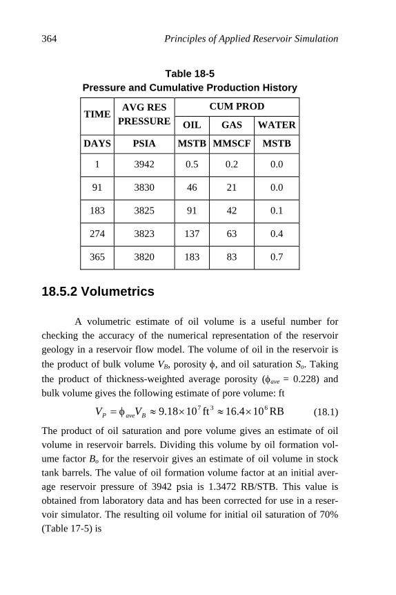
364 Principles of Applied Reservoir Simulation
Table 18-5 Pressure and Cumulative Production History
CUM PROD TIME
AVG RES PRESSURE OIL GAS WATER
DAYS PSIA MSTB MMSCF MSTB
1 3942 0.5 0.2 0.0
91 3830 46 21 0.0
183 3825 91 42 0.1
274 3823 137 63 0.4
365 3820 183 83 0.7
18.5.2 Volumetrics A volumetric estimate of oil volume is a useful number for checking the accuracy of the numerical representation of the reservoir geology in a reservoir flow model. The volume of oil in the reservoir is
the product of bulk volume VB, porosity φ, and oil saturation So. Taking
the product of thickness-weighted average porosity (φave = 0.228) and bulk volume gives the following estimate of pore volume: ft
RB104.16ft1018.9 637 ×≈×≈φ= BaveP VV (18.1)
The product of oil saturation and pore volume gives an estimate of oil volume in reservoir barrels. Dividing this volume by oil formation vol-ume factor Bo for the reservoir gives an estimate of oil volume in stock tank barrels. The value of oil formation volume factor at an initial aver-age reservoir pressure of 3942 psia is 1.3472 RB/STB. This value is obtained from laboratory data and has been corrected for use in a reser-voir simulator. The resulting oil volume for initial oil saturation of 70% (Table 17-5) is
History Matching 365
STB105.8~STBRB3472.1
RB105.11~
7.0 66
××
≈=o
P
o
Poo B
V
B
VSV (18.2)
18.5.3 Material Balance Volumetrics provides one measure of the original fluids in place in a reservoir flow model. Another estimate of original fluids in place can be obtained from a material balance study if a reasonable amount of production data is available, including historical pressure and production data.
Our analysis so far has let us surmise that the reservoir was ini-tially undersaturated. The presence of a few barrels of water during the latter months of the first year of production indicates that mobile water is present, but its source is unknown. The volume of produced water is small enough to be water mobilized by swelling as reservoir pressure declines, or it could be the first indication of water production from aqui-fer influx. Both of these scenarios can be assessed if we consider the possibilities of depletion with and without aquifer influx. We begin by deriving a material balance equation for depletion of an undersaturated oil reservoir with water influx. The derivation is simplified by assuming that formation compressibility is negligible and then setting the decrease in oil volume at reservoir conditions equal to the increase in water volume at reservoir conditions as oil is produced and reservoir pressure decreases. In this case, rock compressibility is 3 × 10⁻⁶ psia-1. For comparison, total compressibility for the DST discussed in Section 17.4 was 13 × 10-6 psia-1. The change in volume due to rock compressibility is considered negligible for the pressure decline range shown in Table 18-5. The material balance equations derived below con-serve volume and neglect volume changes associated with rock compressibility. A more detailed material balance study should include rock compressibility effects.
1. Calculate the decrease in oil volume ∆Vo (RB) given

366 Principles of Applied Reservoir Simulation
N = original oil in place = OOIP (STB)
Boi = oil FVF (RB/STB) at initial pressure Pi
Np = oil produced (STB) at pressure P and time t
Bo = oil FVF (RB/STB) at pressure P and time t
The change in oil volume is
( ) opoio BNNNBV −−=∆ (18.3)
with
NBoi = OOIP (RB) at initial reservoir pressure Pi
(N - Np) Bo = OIP (RB) at pressure P and time t
2. Calculate the increase in water volume ∆Vw (RB) given
W = original water in place = OWIP (RB) at initial pressure Pi
Bw = water FVF (RB/STB) at pressure P and time t
Wp = water produced (STB) at pressure P and time t
We = water influx (RB)
The change in water volume is
( ) wpewpew BWWWBWWWV −=−−+=∆ (18.4)
with
Wp Bw = cumulative water produced (RB) at pressure P and time t
3. The assumption that the volume of the reservoir remains constant im-
plies ∆Vo = ∆Vw. Combining results from steps 1 and 2 above gives the material balance equation for depletion of an incompressible, undersatu-rated oil reservoir with aquifer influx:
( ) wpeopoi BWWBNNNB −=−− (18.5)
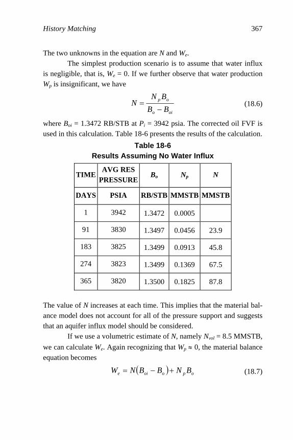
History Matching 367
The two unknowns in the equation are N and We. The simplest production scenario is to assume that water influx is negligible, that is, We = 0. If we further observe that water production Wp is insignificant, we have
oio
op
BB
BNN
−= (18.6)
where Boi = 1.3472 RB/STB at Pi = 3942 psia. The corrected oil FVF is used in this calculation. Table 18-6 presents the results of the calculation.
Table 18-6 Results Assuming No Water Influx
TIMEAVG RES
PRESSUREBo Np N
DAYS PSIA RB/STB MMSTB MMSTB
1 3942 1.3472 0.0005
91 3830 1.3497 0.0456 23.9
183 3825 1.3499 0.0913 45.8
274 3823 1.3499 0.1369 67.5
365 3820 1.3500 0.1825 87.8
The value of N increases at each time. This implies that the material bal-ance model does not account for all of the pressure support and suggests that an aquifer influx model should be considered. If we use a volumetric estimate of N, namely Nvol = 8.5 MMSTB,
we can calculate We. Again recognizing that Wp ≈ 0, the material balance equation becomes
( ) opooie BNBBNW +−= (18.7)

368 Principles of Applied Reservoir Simulation
Table 18-7 shows results of the calculation. Notice that We increases as a function of time. The values in parentheses are IFLO values when the correct aquifer model is used.
Table 18-7 Results Assuming Water Influx with Volumetric OOIP
TIME AVG RES
PRESSUREBo Np We
DAYS PSIA RB/STB MMSTB MMSTB
1 3942 1.3472 0.0005
91 3830 1.3497 0.0456 0.0397 (0.0396)
183 3825 1.3499 0.0913 0.1004 (0.0998)
274 3823 1.3499 0.1369 0.1615 (0.1608)
365 3820 1.3500 0.1825 0.2225 (0.2217)
18.5.4 Relative Permeability As we continue our preparation of a 3-D simulation model, we observe that not all of the data needed by the simulator is available. Since we cannot ignore data and still perform a credible model study, we must complete the data set. Several options are available, such as order-ing additional measurements or finding reasonable correlations or analogies for the missing data. In this case, our commercial interests are best served by moving the project forward without additional expense or delays. We do not have laboratory measured relative permeability data. We could attempt to construct relative permeability data from production data, but our production history is essentially single-phase oil. Since we must specify relative permeability to run the model, we can turn to analogous reservoirs or correlations for guidance. We choose the Honar-pour, et al. [1982] correlation for water-wet sandstone as a starting point
History Matching 369
for determining relative permeability curves. Well logs provide some information about saturation end points such as initial and irreducible water saturation. Core floods and capillary pressure measurements could provide information about residual hydrocarbon saturations, but they are not available. For that reason, end points like residual oil saturation must be estimated. Results of the calculation are included in the case study input data files (data files that begin with “CS”). If our choice of relative permeability correlations does not match field performance, we will have to change the relative permeability curves. In any event, we recognize that in this case study relative permeability is poorly known and should be considered uncertain.
18.5.5 Fluid Contacts A water-oil contact (WOC) was not seen on either well logs or in seismic data. The production of a small amount of water suggests that there may be a WOC in the vicinity of the reservoir. The data are not compelling, however. We could assume that the oil zone extends well below the bottom depth of our well, but this would be an optimistic as-sumption that could prove to be economically disastrous. In the interest of protecting our investment, let us make the more conservative assump-tion that a WOC does exist and is just beyond the range of our
observations, that is, our well log and seismic data. We assume WOC ≈ 9600 ft, which is near the bottom of the seismically observed reservoir structure. The pressure at this WOC depth is estimated to be about 4000 psia.
18.5.6 Grid Preparation Figure 18-2 is a sketch of the well location relative to the inter-preted reservoir boundaries. Based on seismic data shown in Section 17.4, the reservoir is thought to be bounded to the east by a facies change.

370 Principles of Applied Reservoir Simulation
A cross section through points B and B′ shows that the sides of
the reservoir appear to be bounded by faults. Without evidence to the contrary, we assume that the faults are sealing. This assumption is sub-ject to verification during the history match phase of the study.
A cross section through points A and A′ (see Figure 18-2) illus-
trates the dip of the reservoir and the layering. The structure of the reservoir is based on well log and seismic interpretation. The downdip fault is speculative. It is based on the assumption that the fault shown on the western side of Figure 18-2 extends down through the formation. This is not obvious from seismic data. Indeed, if the reservoir is receiv-ing aquifer support, the aquifer influx will come from lower in the reservoir as reservoir pressure declines. Bear in mind, however, that both the fault and the aquifer may be present. This could happen, for example, if the fault is not sealing. The fault could be providing a flow path for water influx from another horizon.
680'Well
P-1A
B
A′
B′
Figure 18-2. Plan View

History Matching 371
Exercises Exercise 18.1 Calculate the pore volume of the reservoir given ∆x =
2000' and ∆y = 1200' from maps, and ∆z = 72' + 96' = 168' from well
logs. Use thickness weighted average porosity. Exercise 18.2A Suppose a well is completed in a gridblock with the fol-
lowing properties: ∆x = ∆y = 200 ft, net thickness = 64 ft, and porosity = 0.25. What is the pore volume of the gridblock in reservoir barrels? Note: 1 bbl = 5.6146 cu ft. Exercise 18.2B If the well is producing 500 RB/day of fluid, what per-centage of the gridblock pore volume is being produced in a 5-day timestep? Exercise 18.3 Data file CS_MB.DAT is an input file for a material bal-ance analysis of the case study. It represents the reservoir as a single gridblock, or "tank” model. The tank model is equivalent to a material balance calculation. Run IFLO with the file CS_MB.DAT. Verify that the original volume of oil in the model agrees with the volumetric esti-mate in Section 18.5. Exercise 18.4 Use data file CS_MB.DAT to study the effect of aquifer influx on material balance performance. This is done by modifying the input data file to include an aquifer model, then adjusting aquifer pa-rameters until model pore volume weighted average reservoir pressures match historical pressures. Note: Section 21.10 contains details on how to set up an analytic aquifer. For an example of a data file with an ana-lytic aquifer model, see data file CS_HM.DAT. Exercise 18.5 Data file CS_VC4.DAT is a vertical column model of the case study. Sketch the grid to scale, locate the contacts on the sketch, and match reservoir pressure. You may need to include an analytic aquifer as in Exercise 18.4.

372 Principles of Applied Reservoir Simulation
Exercise 18.6 Repeat Exercise 18.5 beginning with the cross section model data file CS_XS.DAT.

373
Chapter 19
Predictions The previous chapters have shown how to build a working model of the reservoir and establish a level of confidence in the validity of model results. It is time to recall that modeling was undertaken to pre-pare a tool that would help us develop recommendations for a reservoir management program. The commercial impact of the simulation study is the preparation of a cash flow prediction from projected field perform-ance. Thus, the model study is often completed by making field performance predictions for use in economic analysis of possible operat-ing strategies. This chapter discusses the role of flow models as forecasting tools.
19.1 Prediction Process
The prediction process begins with model calibration. It is usu-ally necessary to ensure continuity in well rate when the modeler switches from rate control during the history match to pressure control during the prediction stage of a study. In Figure 19-1, the solid curve represents the predicted rate based on the productivity index (PI) used in the history match. A clear discontinuity in rate is observed between the end of history and the beginning of prediction. The rate difference usu-ally arises because the actual well PI, especially skin effect, is not

374 Principles of Applied Reservoir Simulation
accurately modeled by the model PI. An adjustment to model PI needs to be made to match final historical rate with initial predicted rate.
adjust PI
PredictionHistory
Rate
Time
Figure 19-1. Model calibration
The next step is to prepare a base case prediction. The base case prediction is a forecast that assumes existing operating conditions apply. For example, the base case for a newly developed field that is undergo-ing primary depletion should be a primary depletion case that extends to a user-specified economic limit. By contrast, if the field was being wa-terflooded, the waterflood should be the base case and alternative strategies might include gas injection and WAG (water alternating gas). The base case prediction establishes a basis from which to com-pare changes in field performance resulting from changes in existing operating conditions. In addition, a sensitivity analysis should be per-formed to provide insight into the uncertainty associated with model predictions. A procedure for conducting a sensitivity analysis is outlined below.
19.2 Sensitivity Analyses Sensitivity analyses are often needed in both the history match-ing and prediction stages [for example, see Crichlow, 1977; Mattax and Dalton, 1990; Saleri, 1993; Fanchi, et al., 1996; Carlson, 2003]. Any

Predictions 375
method that quantifies the uncertainty or risk associated with selecting a particular prediction case may be viewed as a sensitivity analysis. Con-ceptual modeling is an example of a sensitivity analysis technique that is cost-effective in moving a history match forward. It can be used to ad-dress very specific questions, such as determining the impact of fluid contact movement on hydrocarbon recovery. Similarly, window models that study such issues as the behavior of a horizontal well in a fault block provide useful information on the sensitivity of a model to changes in input parameters. Another example of a sensitivity analysis technique is risk analy-sis. Murtha [1997] defines risk analysis as “any form of analysis that studies and hence attempts to quantify risks associated with an invest-ment.” Risk in this context refers to a potential “change in assets associated with some chance occurrences.” Risk analysis generates prob-abilities associated with changes in model input parameters. The parameter changes must be contained within ranges that are typically determined by the range of available data, information from analogous fields, and the experience of the modeling team. Each model run using a complete set of model input parameters constitutes a trial. A large num-ber of trials can be used to generate probability distributions. Alternatively, the results of the trials can be used in a multivariable re-gression analysis to generate analytical expressions, as described below. One of the most widely used techniques for studying model sen-sitivity to input parameter changes is to modify model input parameters in the history matched model. The following procedure combines multi-variable regression and the results of model trials to generate an analytical expression for quantifying the effect of changing model pa-rameters. Assume a dependent variable F has the form
∏=
κ=n
j
ej
jXF1
(19.1)
where {Xj} are n independent variables and κ is a proportionality con-stant that depends on the units of the independent variables. Examples of Xj are well separation, saturation end points, and aquifer strength. Taking
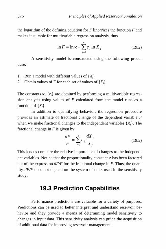
376 Principles of Applied Reservoir Simulation
the logarithm of the defining equation for F linearizes the function F and makes it suitable for multivariable regression analysis, thus
∑=
+κ=n
jjj XeF
1
lnlnln (19.2)
A sensitivity model is constructed using the following proce-dure: 1. Run a model with different values of {Xj} 2. Obtain values of F for each set of values of {Xj}
The constants κ, {ej} are obtained by performing a multivariable regres-
sion analysis using values of F calculated from the model runs as a function of {Xj}. In addition to quantifying behavior, the regression procedure provides an estimate of fractional change of the dependent variable F when we make fractional changes to the independent variables {Xj}. The fractional change in F is given by
∑=
=n
j j
jj X
dXe
F
dF
1
(19.3)
This lets us compare the relative importance of changes to the independ-
ent variables. Notice that the proportionality constant κ has been factored
out of the expression dF/F for the fractional change in F. Thus, the quan-tity dF/F does not depend on the system of units used in the sensitivity study.
19.3 Prediction Capabilities Performance predictions are valuable for a variety of purposes. Predictions can be used to better interpret and understand reservoir be-havior and they provide a means of determining model sensitivity to changes in input data. This sensitivity analysis can guide the acquisition of additional data for improving reservoir management.

Predictions 377
Predictions enable people to estimate project life by predicting recovery versus time. Project life depends not only on the flow behavior of the reservoir, but also on commercial issues. Models let the user im-pose a variety of economic constraints on future reservoir performance during the process of estimating project life. These constraints reflect a range of economic criteria that will interest management, shareholders, and prospective investors. Commercial interests are clearly important to the future of a pro-ject, as are technical issues. It is often necessary to compare different recovery processes as part of a study. Since there is only one field, it is unrealistic to believe that many different recovery processes can be evaluated in the field, even as small scale pilot projects. Pilot projects tend to be substantially more expensive to run than simulation studies. In some cases, however, it might be worthwhile to confirm a simulation study with a pilot project. This is especially true with expensive proc-esses such as chemical and thermal flooding. Yet another use for model predictions is the preparation of a res-ervoir management plan. Reservoir management plans have been discussed in previous sections. Their preparation is often the single most important motivation for performing a simulation study.
19.3.1 Economic Analysis In addition to providing technical insight into fluid flow per-formance, model predictions are frequently combined with price forecasts to estimate how much revenue will be generated by a proposed reservoir management plan. The revenue stream is used to pay for capital and operating expenses, and the economic performance of the project depends on the relationship between revenue and expenses [see, for ex-ample, Chorn and Croft, 2000; Seba, 1998; Bradley and Wood, 1994; Mian, 1992; Thompson and Wright, 1985]. In a very real sense, the reservoir flow model determines how much money will be available to pay for wells, compressors, pipelines, platforms, processing facilities, and any other items needed to implement
378 Principles of Applied Reservoir Simulation
the plan represented by the model. For this reason, the modeling team may be expected to generate flow predictions using a combination of reservoir parameters that yield better recoveries than would be expected if a less “optimistic” set of parameters had been used. The sensitivity analysis is a useful process for determining the likelihood that a set of parameters will be realized. Indeed, modern reserves classification sys-tems are designed to present reserves estimates in terms of their probability of occurrence. The probabilistic representation of forecasts gives decision-making bodies such as corporate managements and finan-cial institutions the information they need to make informed decisions.
19.4 Validity of Model Predictions Saleri [1993] studied the validity of model predictions by com-paring actual field performance with predicted performance. The overall match of field performance, such as total rate and pressure performance, is reasonable. The field match is somewhat deceptive however, because the validity of individual well performance forecasting varies widely. Indeed, Saleri deemed the match of water and gas performance for about half of the wells a “bust” by the author. This is not unusual in a model study. Saleri arrived at the following conclusions:
Ü “Barring major geologic and/or reservoir data limitations, fieldwide cumulative production forecast accuracies would tend to range from 10% to 40%.” [Saleri, 1993]
Ü “Well performance forecasts are bound to be less successful than fieldwide predictions.” [Saleri, 1993]
These points underscore the need to recognize that the history match process does not yield a unique solution. Forecasts of reservoir behavior depend on the validity of the history match. Despite the uncertainty associated with simulator-based fore-casts, reservoir simulation continues to be the most reliable method for making performance predictions, particularly for reservoirs that do not have an extensive history or for fields that are being considered as candi-dates for a change in reservoir management strategy. Other methods,

Predictions 379
such as decline curve analysis and material balance analysis, can gener-ate performance forecasts, but not to the degree of detail provided by a reservoir flow model study. As Saleri [1993] noted,
Ü “While a 10% to 40% forecast uncertainty may appear alarming in an absolute sense, the majority of reservoir en-gineering decisions require choices based solely on comparative analyses (for example, peripheral vs. pattern flood). Thus, in selecting optimum management strategies, finite difference models still offer the most effective tools.”
Saleri’s view is similar to that of Oreskes, et al. [1994]. Even though models are nonunique representations of nature, they still have many uses. In summary, models can be used to
Ü Corroborate or refute hypotheses about physical systems Ü Identify discrepancies in other models Ü Perform sensitivity analyses
19.5 Case Study: History Match and Prediction
The history match is now well under way. The models discussed in the exercises in Chapter 18 are conceptual models designed to provide you with a sense of how fluids move in the reservoir. This is the art of modeling. As you work with various models of the reservoir, you should begin to develop a knowledge base for determining how changes to model parameters will help achieve a match for a particular physical variable. This knowledge base is valuable as you develop your feel for the study. The previous chapters set the stage for preparing a 3-D model of the case study reservoir. A 3-D model should provide enough reservoir definition to let us make meaningful performance predictions. Before matching the 3-D model, we discuss how to incorporate well information into the model. Once the well model has been prepared, we proceed to history matching and performance predictions.

380 Principles of Applied Reservoir Simulation
19.5.1 Well Model Preparation Well model calculations require estimates of productivity index and flowing bottomhole pressure. This section illustrates these calcula-tions.
19.5.1.1 Productivity Index Estimate
Well model calculations in IFLO need to have the quasistation-ary productivity index factor (PID) specified by the user. PID is estimated from the expression
( ) Srr
hKPID
we
netabs
+=
ln
00708.0 (19.4)
where
re = drainage radius (ft)
rw = wellbore radius (ft)
S = skin
K e = kroKabs = effective permeability (md)
hnet = net thickness (ft)
Given S = -0.5, rw = 0.25 ft and
( ) ft4014.0 21
22 ≅∆+∆≅ yxro (19.5)
with ∆x = ∆y = 200 ft., we find
netabshKPID 31055.1 −×= (19.6)
where re ≈ ro. Table 19-1 presents the calculation of PID for each layer identified by well log analysis. Notice that the second model layer has no flow capacity because the model layer represents impermeable shale. The upper sand is represented by the first model layer, and the lower sand is represented by the third and fourth model layers.
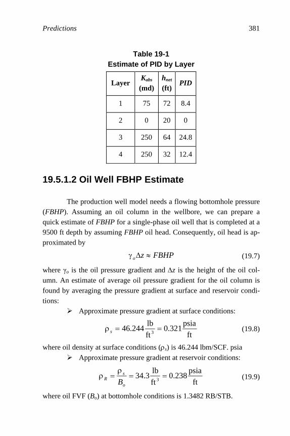
Predictions 381
Table 19-1 Estimate of PID by Layer
Layer Kabs (md)
hnet
(ft)PID
1 75 72 8.4
2 0 20 0
3 250 64 24.8
4 250 32 12.4
19.5.1.2 Oil Well FBHP Estimate
The production well model needs a flowing bottomhole pressure (FBHP). Assuming an oil column in the wellbore, we can prepare a quick estimate of FBHP for a single-phase oil well that is completed at a 9500 ft depth by assuming FBHP oil head. Consequently, oil head is ap-proximated by
FBHPzo ≈∆γ (19.7)
where けo is the oil pressure gradient and ∆z is the height of the oil col-umn. An estimate of average oil pressure gradient for the oil column is found by averaging the pressure gradient at surface and reservoir condi-tions:
Ü Approximate pressure gradient at surface conditions:
ft
psia321.0
ft
lb244.46
3==ρs (19.8)
where oil density at surface conditions (ρs) is 46.244 lbm/SCF. psia Ü Approximate pressure gradient at reservoir conditions:
ft
psia238.0
ft
lb3.34
3==
ρ=ρ
o
sR B
(19.9)
where oil FVF (Bo) at bottomhole conditions is 1.3482 RB/STB.

382 Principles of Applied Reservoir Simulation
The resulting FBHP for use in IFLO is
psia2660
ft9500ft
psia238.0
ft
psia321.0
2
1FBHP
≈
×⎥⎦
⎤⎢⎣
⎡+=
(19.10)
A more accurate estimate can be obtained from wellbore correlations or nodal analysis as discussed by such authors as Brown and Lea [1985].
19.5.1.3 Well Gridblock Pressure from PBU A correction is needed to properly relate the pressure buildup (PBU) curve to simulator well gridblock pressures. To illustrate this cor-
rection, suppose a well is in a gridblock with grid dimensions ∆x = 200 ft
and ∆y = 200 ft. We want to compare the simulator well gridblock pres-sure with a pressure from a PBU. According to Peaceman’s correction [1978, 1983], shut-in pressure Pws of the actual well should equal the
simulator well gridblock pressure Po at a shut-in time ∆ts given by
K
rct oT
s
21688φµ=∆ (19.11)
For an isotropic reservoir in which horizontal permeability does not de-pend on direction, that is, Kx = Ky, we estimate the equivalent radius of a well in the center of a gridblock as
( ) 21
2214.0 yxro ∆+∆= (19.12)
The shut in time ∆ts at which the PBU pressure should be obtained is
calculated from the following physical parameters:
cr 3 × 10⁻⁶ psia-1
co 13 × 10-6 psia-1
cw 3 × 10⁻⁶ psia-1
So 0.7

Predictions 383
Sw 0.3
µo 0.71 cp
φ 0.20
K 75 md
The equivalent radius of the well gridblock is estimated to be ro
≈ 0.14 (2002 + 2002)½ = 39.6 ft, while the total compressibility is given
by cT = cr + So co + Sw cw = 3 × 10⁻⁶ + 0.7 (13 × 10-6) + 0.3 (3 × 10⁻⁶)
≈ 13 × 10-6 psia-1. The PBU shut in time corresponding to these values is
( )( )( )( )
min4hr065.0
75
6.39101371.020.01688
26
==
×=∆
−
st (19.13)
This early time part of the PBU curve could be masked by wellbore stor-age effects. Since the shut in pressure Pws of the actual well equals the
simulator well gridblock pressure Po at a shut in time ∆ts, the shut in pressure Pws may have to be obtained by extrapolation of the radial flow curve.
19.5.1.3.1 Throughput Estimate
Model timestep size is estimated by calculating pore volume throughput from well flow rates. In our case, pore volume throughput is given by
( )6146.5P
PT V
tQV
∆= (19.14)
where
VP = φ ∆x ∆y ∆z = pore volume (ft3)
Q = volumetric flow rate at reservoir conditions (RB/day)

384 Principles of Applied Reservoir Simulation
∆t = timestep size (day)
Timesteps for an IMPES simulator should correspond to about 10% throughput or less. The maximum timestep is estimated as follows.
Suppose φ = 22.5%, ∆x = ∆y = 200 ft, ∆z = hnet, and Q = 400
RB/day. Then ∆t is found by setting VPT = 0.10 and rearranging the pore volume throughput equation to give
( ) ( ) ( )days4.0
6146.51.0
6146.5
1.0net
P hQ
zyx
Q
Vt =
∆∆∆φ==∆ (19.15)
If hnet = 100 ft, then ∆t ≈ 40 days is an estimate of the maximum IMPES timestep size.
19.5.2 Full Field (3-D) Model History Match
Data file CS_HM.DAT is the 3-D model used to match the pro-duction history. It uses the areal grid shown in Figure 19-2 to model the reservoir. Production well P-1 and its location in the grid are also shown
in Figure 19-2. Each gridblock is a square with lengths ∆x = ∆y = 200 ft.
The dark areas of the grid are outside the reservoir area. The pore vol-ume in the dark area is made inactive in data file CS_HM.DAT by using porosity multipliers.
P-1
Figure 19-2. Plan View of Grid

Predictions 385
The depth and thickness of each gridblock depend on reservoir architecture. The model grid should approximate the structure depicted in Figure 17-9. The dip of the reservoir is included by specifying the tops of each gridblock. The gridblock length modifications are designed to cut off those parts of the gridblock that continue the grid beyond the sur-face of the unconformity sketched. Transmissibility multipliers in the vertical direction are set to zero to simulate impermeable shale barriers. This includes the shale streak that divides the second major sand into two thinner sands with a shale break. The interpretation of seismic data was unable to resolve this feature, but the well log shown in Figure 19-3 does indicate the presence of a shale streak.
Figure 19-3. Overlay of Seismic and Well Log Data
The water-oil contact is at 9600 ft. A steady-state aquifer is in
communication with all three oil layers at this depth. It is the source of water production shown in the production history.

386 Principles of Applied Reservoir Simulation
19.5.3 Predictions Predictions can be made once a history match model is adopted. The first step in the prediction stage is to establish a base case prediction. A frequently used base case is one that assumes that there will be no changes in operating strategy. Given a base case prediction, several runs should be made to optimize reservoir performance within the constraints imposed by the commissioners of the study and to evaluate the sensitiv-ity of predictions to data limitations. In our case, the predictions should satisfy the reservoir management constraints in Table 17-10. Production forecasts can then be combined with price forecasts to predict cash flow, and provide valuable economic information to decision makers.
Exercises Exercise 19.1 Repeat the shut in time ∆ts calculation in Section 19.5.1
using ∆x = 1000 ft and ∆y = 1000 ft.
Exercise 19.2A Run data file CS_XS.DAT and estimate the average timestep size of the run. Is there an analytic aquifer in the model? Exercise 19.2B What are the average reservoir pressure and water pro-duction rate at the end of the run? How do these results compare with the historical data presented in Section 18.5? Exercise 19.3A Attach a steady-state analytic aquifer model to both lay-ers in the first (I = 1) column of data file CS_XS.DAT. Set the aquifer strength equal to 2 SCF/day/psia. What is your final average reservoir pressure, water production rate, and aquifer influx rate? Exercise 19.3B How do your results compare with the historical data presented in Section 18.5 and the results of Exercise 19.2?
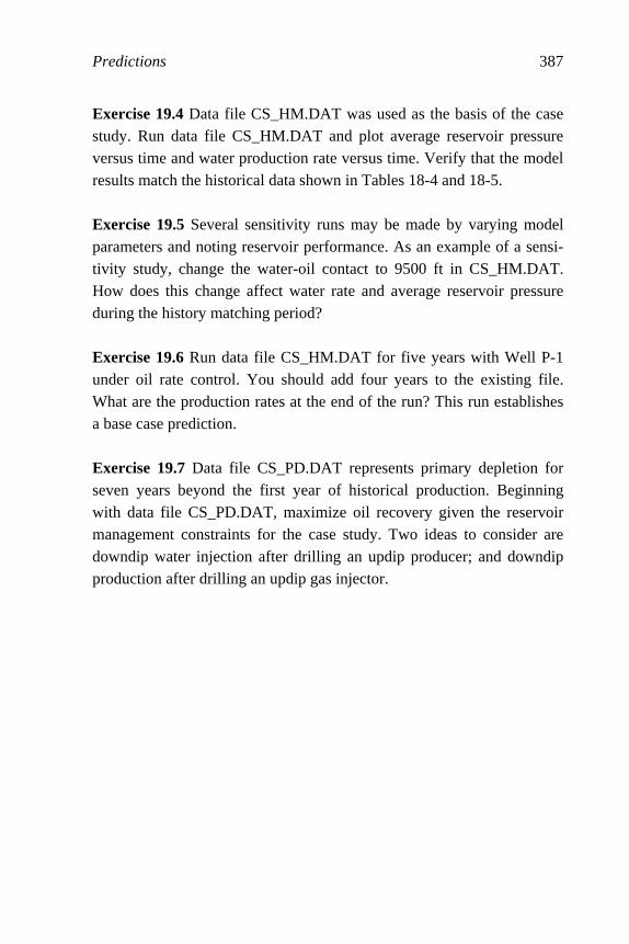
Predictions 387
Exercise 19.4 Data file CS_HM.DAT was used as the basis of the case study. Run data file CS_HM.DAT and plot average reservoir pressure versus time and water production rate versus time. Verify that the model results match the historical data shown in Tables 18-4 and 18-5. Exercise 19.5 Several sensitivity runs may be made by varying model parameters and noting reservoir performance. As an example of a sensi-tivity study, change the water-oil contact to 9500 ft in CS_HM.DAT. How does this change affect water rate and average reservoir pressure during the history matching period? Exercise 19.6 Run data file CS_HM.DAT for five years with Well P-1 under oil rate control. You should add four years to the existing file. What are the production rates at the end of the run? This run establishes a base case prediction. Exercise 19.7 Data file CS_PD.DAT represents primary depletion for seven years beyond the first year of historical production. Beginning with data file CS_PD.DAT, maximize oil recovery given the reservoir management constraints for the case study. Two ideas to consider are downdip water injection after drilling an updip producer; and downdip production after drilling an updip gas injector.

388
Chapter 20
Introduction to IFLO
IFLO is an iterative, implicit pressure-explicit saturation finite difference simulator. It can simulate isothermal, multiphase Darcy flow in up to three dimensions. This chapter outlines procedures for entering data into IFLO, executing IFLO, and obtaining results from IFLO.
20.1 Input Data File
IFLO input data is divided into two parts: initialization data, and recurrent data. Chapter 21 describes initialization data which include data that is set at the beginning of the study and is not expected to change during a model run. Such data includes the reservoir description and fluid properties. Chapter 22 describes recurrent data which include data that are expected to change during the course of a simulation. Such data include well schedules and timestep control information. Appendix B presents an example input data set.
IFLO reads a file called ITEMP.DAT and outputs to files with the prefix ITEMP. The output files are described below. You should copy and rename any files you wish to save because IFLO overwrites the ITEMP.* files each time it runs.
An efficient way to prepare a new data file is to edit an old one. This will give you an example of the formats needed for most options. If

Introduction to IFLO 389
you start with an old data set, make sure that you check all applicable data entries and make changes where appropriate.
20.2 IFLO Execution
You are given the option at the start of an IFLO run to direct output to either the screen or to a set of files. The program IFLO runs the file called ITEMP.DAT. To run a new data set, such as NEWDATA.DAT, copy NEWDATA.DAT to ITEMP.DAT. The File ITEMP.DAT should be in the same folder as the executable IFLO.EXE.
Run IFLO by double-clicking on the IFLO.EXE file. Select op-tion “Y” to write the run output to files. A one-line timestep summary is sent to the screen each timestep so that you can monitor the progress of a run. When the program ends, it will print “STOP.” Close the IFLO win-dow. You do not need to save changes since they are written to file ITEMP.TSS. All output files are in text format.
It is often worthwhile to send output to the screen when first building and debugging a data set. To implement this option, double-click on the IFLO.EXE file and select option “N” to write the run output to the screen. IFLO will abort at the point in the data set where it encoun-ters improperly entered data. For evaluating run results, it is preferable to send output to files.
20.3 IFLO Output Files
All IFLO output files are text files so that they may be read by a variety of commercially available spreadsheets. IFLO output may then be manipulated using spreadsheet options. This is especially useful for making plots or displaying array data. Different output files are defined so that simulator output file sizes are more manageable. The output files are designed to contain information that is logically connected, e.g. well data in one file, timestep information in another file. The different output files are described below.
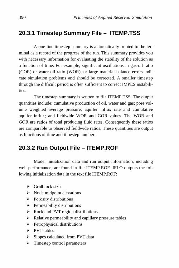
390 Principles of Applied Reservoir Simulation
20.3.1 Timestep Summary File – ITEMP.TSS
A one-line timestep summary is automatically printed to the ter-minal as a record of the progress of the run. This summary provides you with necessary information for evaluating the stability of the solution as a function of time. For example, significant oscillations in gas-oil ratio (GOR) or water-oil ratio (WOR), or large material balance errors indi-cate simulation problems and should be corrected. A smaller timestep through the difficult period is often sufficient to correct IMPES instabili-ties.
The timestep summary is written to file ITEMP.TSS. The output quantities include: cumulative production of oil, water and gas; pore vol-ume weighted average pressure; aquifer influx rate and cumulative aquifer influx; and fieldwide WOR and GOR values. The WOR and GOR are ratios of total producing fluid rates. Consequently these ratios are comparable to observed fieldwide ratios. These quantities are output as functions of time and timestep number.
20.3.2 Run Output File – ITEMP.ROF
Model initialization data and run output information, including well performance, are found in file ITEMP.ROF. IFLO outputs the fol-lowing initialization data in the text file ITEMP.ROF:
Ü Gridblock sizes Ü Node midpoint elevations Ü Porosity distributions Ü Permeability distributions Ü Rock and PVT region distributions Ü Relative permeability and capillary pressure tables Ü Petrophysical distributions Ü PVT tables Ü Slopes calculated from PVT data Ü Timestep control parameters

Introduction to IFLO 391
Ü Analytic aquifer model selection Ü Coal gas model selection Ü Initial fluid volumes-in-place Ü Initial pressure and saturation arrays Ü Initial reservoir geophysical attribute arrays Ü Initial well information
Other output can be obtained at your request. For example, if a modifica-tion option is invoked, you may print out the altered array. It is worthwhile to do this as a check on the input changes.
You may output the following arrays whenever you desire as part of the recurrent data output: pressure, saturations, bubble point pres-sure, cumulative aquifer influx, acoustic velocities, acoustic impedances, seismic reflection coefficient, Poisson’s ratio, Young’s modulus, and uniaxial compaction. Output arrays may be used as input pressure and saturation distributions for restarting a run.
It is usually unnecessary to print all of the arrays. To avoid ex-cessive output and correspondingly large output files, you should decide judiciously which arrays to print.
20.3.3 Well Output File – ITEMP.WEL
Well performance data are found in file ITEMP.WEL. The in-formation is provided for easy access and includes production (injection) for each well completion as well as total well production (injection) for all production (injection) wells.
20.3.4 Array File – ITEMP.ARR
Selected parameter arrays are tabulated in ITEMP.ARR. The ar-rays are displayed as functions of the Cartesian (x, y, z) coordinate locations of each gridblock midpoint. The parameter arrays include pres-sure, saturations, and acoustic velocity information.

392 Principles of Applied Reservoir Simulation
20.3.5 Material Balance Error File – ITEMP.MBE
Material balance errors as a function of time are summarized in ITEMP.MBE.

393
Chapter 21
Initialization Data
Initialization data records are read once at the beginning of the simulation. They must be read in the order presented below. Title or heading records are read before each major and many minor sections. These records are designed to make the input data file easier to read and edit.
In many cases, codes are read that will specify the type of input to follow and the number of values that will be read. These codes in-crease the efficiency and flexibility of entering input data. All input data, with the exception of well names, are entered by free format. Data en-tered on the same line must be separated by a comma or a space.
Tabular data entered by the user should cover the entire range of values expected to occur during a simulation. The table interpolation al-gorithms in IFLO will return table endpoint values if the independent variable goes outside the range of the input tabular values. No message will be printed if this occurs. 1. Title Up to 80 characters. This record will appear as run title.

394 Principles of Applied Reservoir Simulation
21.1 Model Dimensions and Geometry
21.1.1 Model Dimensions 1. Heading Up to 80 characters. 2. II, JJ, KK, NWELL, NWCON
Code Meaning
II number of gridblocks in the x-direction
JJ number of gridblocks in the y-direction
KK number of gridblocks in the z-direction
NWELL number of wells
NWELCON number of connections per well
NOTE: The IFLO simulator assumes a block centered grid with the axes aligned using a right-handed coordinate system with the z-axis pointing down. The top layer is labeled by the index K = 1. The second layer K = 2 is below the K = 1 layer, and so on.
3. Heading Up to 80 characters. 4. KDX, KDY, KDZ, KDZNET
KDX Control code for input of x-direction grid size. KDY Control code for input of y-direction grid size. KDZ Control code for input of z-direction gross
thickness. KDZNET Control code for input of z-direction net thick-
ness.
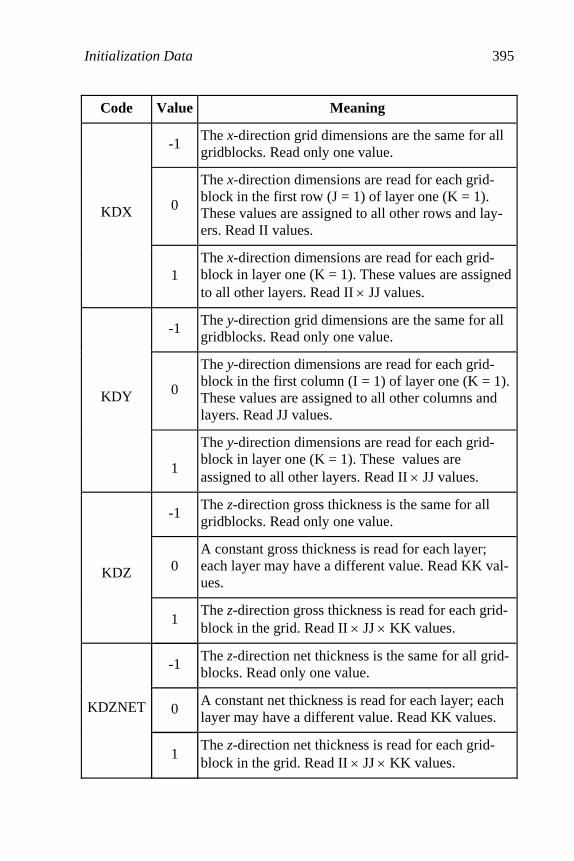
Initialization Data 395
Code Value Meaning
-1 The x-direction grid dimensions are the same for all gridblocks. Read only one value.
0
The x-direction dimensions are read for each grid-block in the first row (J = 1) of layer one (K = 1). These values are assigned to all other rows and lay-ers. Read II values.
KDX
1 The x-direction dimensions are read for each grid-block in layer one (K = 1). These values are assigned to all other layers. Read II × JJ values.
-1 The y-direction grid dimensions are the same for all gridblocks. Read only one value.
0
The y-direction dimensions are read for each grid-block in the first column (I = 1) of layer one (K = 1). These values are assigned to all other columns and layers. Read JJ values.
KDY
1
The y-direction dimensions are read for each grid-block in layer one (K = 1). These values are assigned to all other layers. Read II × JJ values.
-1 The z-direction gross thickness is the same for all gridblocks. Read only one value.
0 A constant gross thickness is read for each layer; each layer may have a different value. Read KK val-ues.
KDZ
1 The z-direction gross thickness is read for each grid-block in the grid. Read II × JJ × KK values.
-1 The z-direction net thickness is the same for all grid-blocks. Read only one value.
0 A constant net thickness is read for each layer; each layer may have a different value. Read KK values.
KDZNET
1 The z-direction net thickness is read for each grid-block in the grid. Read II × JJ × KK values.

396 Principles of Applied Reservoir Simulation
NOTE: If an array of input values must be read, the following input order must be followed. Layer 1 (K = 1) is read first. The data in each layer are read by the rows, starting with row 1 (J = 1). Values of the array element are read for the first row starting with column 1 (I = 1) and proceeding to the end of the row (col-umn I = II). After II values are read, the next row (J = 2) of values are entered. These values must begin on a new line. This data entry procedure is repeated for all rows and, subsequently, for all layers until the complete set of array elements has been entered.
5. DX
DX Gridblock size in x-direction (ft). If KDX = -1, read one constant value. If KDX = 0, read II values (one for each row).
If KDX = +1, read II × JJ values (one for each K = 1 grid-block).
6. DY
DY Gridblock size in y-direction (ft). If KDY = -1, read one constant value. If KDY = 0, read JJ values (one for each column).
If KDY = +1, read II × JJ values (one for each K = 1 grid-
block). 7. DZ
DZ Gross gridblock thickness in z-direction (ft). If KDZ = -1, read one constant value. If KDZ = 0, read KK values (one for each layer).
If KDZ = +1, read II × JJ × KK values (one for each grid-
block). 8. DZNET
DZNET Net gridblock thickness in z-direction (ft).
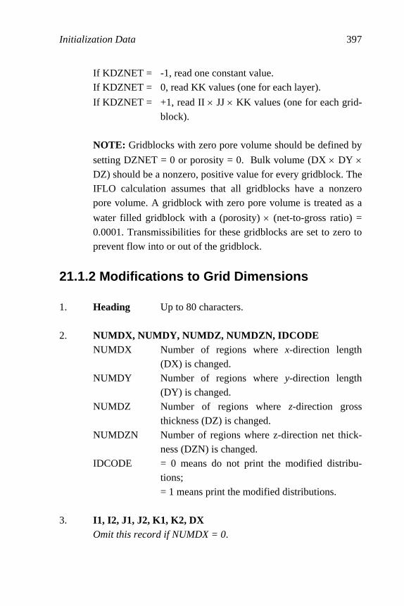
Initialization Data 397
If KDZNET = -1, read one constant value. If KDZNET = 0, read KK values (one for each layer).
If KDZNET = +1, read II × JJ × KK values (one for each grid-block).
NOTE: Gridblocks with zero pore volume should be defined by
setting DZNET = 0 or porosity = 0. Bulk volume (DX × DY ×
DZ) should be a nonzero, positive value for every gridblock. The IFLO calculation assumes that all gridblocks have a nonzero pore volume. A gridblock with zero pore volume is treated as a
water filled gridblock with a (porosity) × (net-to-gross ratio) = 0.0001. Transmissibilities for these gridblocks are set to zero to prevent flow into or out of the gridblock.
21.1.2 Modifications to Grid Dimensions 1. Heading Up to 80 characters. 2. NUMDX, NUMDY, NUMDZ, NUMDZN, IDCODE
NUMDX Number of regions where x-direction length (DX) is changed.
NUMDY Number of regions where y-direction length (DY) is changed.
NUMDZ Number of regions where z-direction gross thickness (DZ) is changed.
NUMDZN Number of regions where z-direction net thick-ness (DZN) is changed.
IDCODE = 0 means do not print the modified distribu-tions; = 1 means print the modified distributions.
3. I1, I2, J1, J2, K1, K2, DX
Omit this record if NUMDX = 0.

398 Principles of Applied Reservoir Simulation
I1 Coordinate of first region gridblock in I-direction.
I2 Coordinate of last region gridblock in I-direction.
J1 Coordinate of first region gridblock in J-direction.
J2 Coordinate of last region gridblock in J-direction.
K1 Coordinate of first region gridblock in K-direction.
K2 Coordinate of last region gridblock in K-direction.
DX New value of x-direction grid size for region (ft).
NOTE: NUMDX records must be read.
4. I1, I2, J1, J2, K1, K2, DY
Omit this record if NUMDY = 0. I1 Coordinate of first region gridblock in I-
direction. I2 Coordinate of last region gridblock in I-
direction. J1 Coordinate of first region gridblock in J-
direction. J2 Coordinate of last region gridblock in J-
direction. K1 Coordinate of first region gridblock in K-
direction. K2 Coordinate of last region gridblock in K-
direction. DY New value of y-direction grid size for region
(ft).
NOTE: NUMDY records must be read.
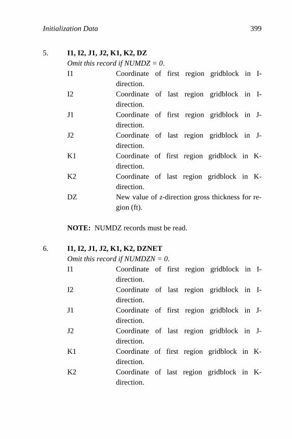
Initialization Data 399
5. I1, I2, J1, J2, K1, K2, DZ Omit this record if NUMDZ = 0. I1 Coordinate of first region gridblock in I-
direction. I2 Coordinate of last region gridblock in I-
direction. J1 Coordinate of first region gridblock in J-
direction. J2 Coordinate of last region gridblock in J-
direction. K1 Coordinate of first region gridblock in K-
direction. K2 Coordinate of last region gridblock in K-
direction. DZ New value of z-direction gross thickness for re-
gion (ft).
NOTE: NUMDZ records must be read. 6. I1, I2, J1, J2, K1, K2, DZNET
Omit this record if NUMDZN = 0. I1 Coordinate of first region gridblock in I-
direction. I2 Coordinate of last region gridblock in I-
direction. J1 Coordinate of first region gridblock in J-
direction. J2 Coordinate of last region gridblock in J-
direction. K1 Coordinate of first region gridblock in K-
direction. K2 Coordinate of last region gridblock in K-
direction.

400 Principles of Applied Reservoir Simulation
DZNET New value of z-direction net thickness for re-gion (ft).
NOTE: NUMDZN records must be read.
21.1.3 Depths to Top of Gridblocks
The coordinate system used in IFLO is defined so that values in the z-direction (vertical) increase as the layer gets deeper. Negative val-ues will be read as heights above the datum. 1. Heading Up to 80 characters. 2. KEL KEL Control code for input of depth values.
KEL Meaning
0
A single constant value is read for the depth to the top of all grid-blocks in layer 1 (horizontal plane). Each layer is contiguous in this option. Depths to the top of gridblocks in layers below layer 1 are calculated by adding the layer thickness to the preceding layer top; thus Top (I, J, K + 1) = Top (I, J, K) + DZ (I, J, K)
1
A separate depth value must be read for each gridblock in layer 1. Read II × JJ values. Each layer is contiguous in this option. Depths to the top of gridblocks in layers below layer 1 are calcu-lated by adding the layer thickness to the preceding layer top; thus Top (I, J, K + 1) = Top (I, J, K) + DZ (I, J, K)
2 A separate depth value is read for each layer. Read KK values. Each layer is horizontal (layer cake) in this option.
3 A separate depth value is read for each gridblock. Read II × JJ × KK values.
3. ELEV
ELEV Depth to top of gridblock (ft).
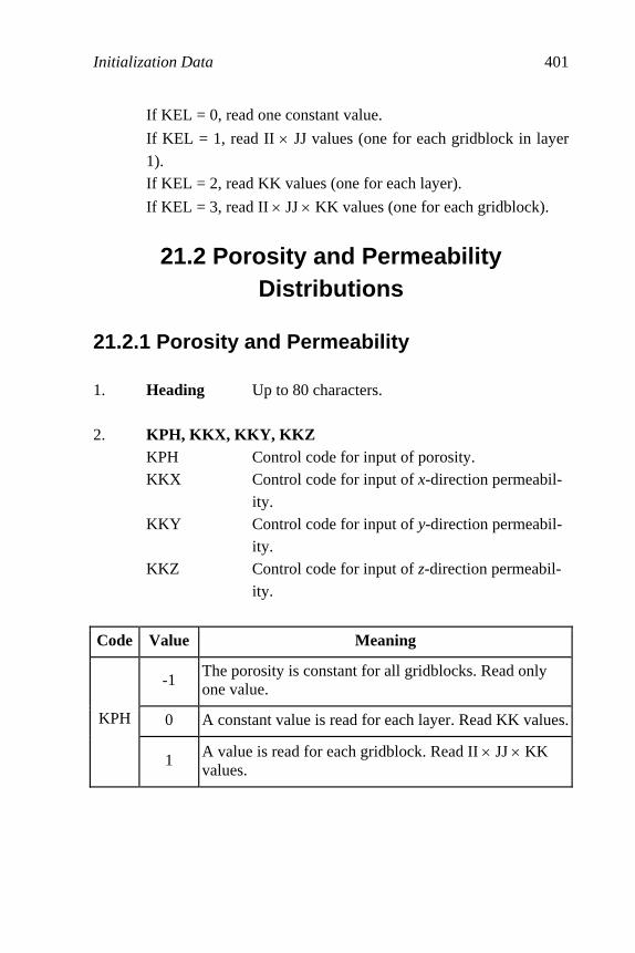
Initialization Data 401
If KEL = 0, read one constant value.
If KEL = 1, read II × JJ values (one for each gridblock in layer
1). If KEL = 2, read KK values (one for each layer).
If KEL = 3, read II × JJ × KK values (one for each gridblock).
21.2 Porosity and Permeability Distributions
21.2.1 Porosity and Permeability 1. Heading Up to 80 characters. 2. KPH, KKX, KKY, KKZ
KPH Control code for input of porosity. KKX Control code for input of x-direction permeabil-
ity. KKY Control code for input of y-direction permeabil-
ity. KKZ Control code for input of z-direction permeabil-
ity.
Code Value Meaning
-1 The porosity is constant for all gridblocks. Read only one value.
0 A constant value is read for each layer. Read KK values. KPH
1 A value is read for each gridblock. Read II × JJ × KK values.

402 Principles of Applied Reservoir Simulation
-1 The x-direction permeability is constant for all grid-blocks. Read only one value.
0 A constant value is read for each layer. Read KK values.KKX
1 A value is read for each gridblock. Read II × JJ × KK values.
-1 The y-direction permeability is constant for all grid-blocks. Read only one value.
0 A constant value is read for each layer. Read KK values.KKY
1 A value is read for each gridblock. Read II × JJ × KK values.
-1 The z-direction permeability is constant for all grid-blocks. Read only one value.
0 A constant value is read for each layer. Read KK values.KKZ
1 A value is read for each gridblock. Read II × JJ × KK values.
3. PHI
PHI Porosity (fraction). If KPH = -1, read one constant value. If KPH = 0, read KK values (one for each layer).
If KPH = +1, read II × JJ × KK values (one for each grid-
block). 4. PERMX
PERMX Permeability in x-direction (md). If KKX = -1, read one constant value. If KKX = 0, read KK values (one for each layer).
If KKX = +1, read II × JJ × KK values (one for each grid-block).
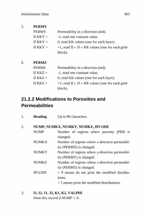
Initialization Data 403
5. PERMY PERMY Permeability in y-direction (md). If KKY = -1, read one constant value. If KKY = 0, read KK values (one for each layer).
If KKY = +1, read II × JJ × KK values (one for each grid-block).
6. PERMZ
PERMZ Permeability in z-direction (md). If KKZ = -1, read one constant value. If KKZ = 0, read KK values (one for each layer).
If KKZ = +1, read II × JJ × KK values (one for each grid-
block).
21.2.2 Modifications to Porosities and Permeabilities 1. Heading Up to 80 characters. 2. NUMP, NUMKX, NUMKY, NUMKZ, IPCODE
NUMP Number of regions where porosity (PHI) is changed.
NUMKX Number of regions where x-direction permeabil-ity (PERMX) is changed.
NUMKY Number of regions where y-direction permeabil-ity (PERMY) is changed.
NUMKZ Number of regions where z-direction permeabil-ity (PERMZ) is changed.
IPCODE = 0 means do not print the modified distribu-tions; = 1 means print the modified distributions.
3. I1, I2, J1, J2, K1, K2, VALPHI
Omit this record if NUMP = 0.
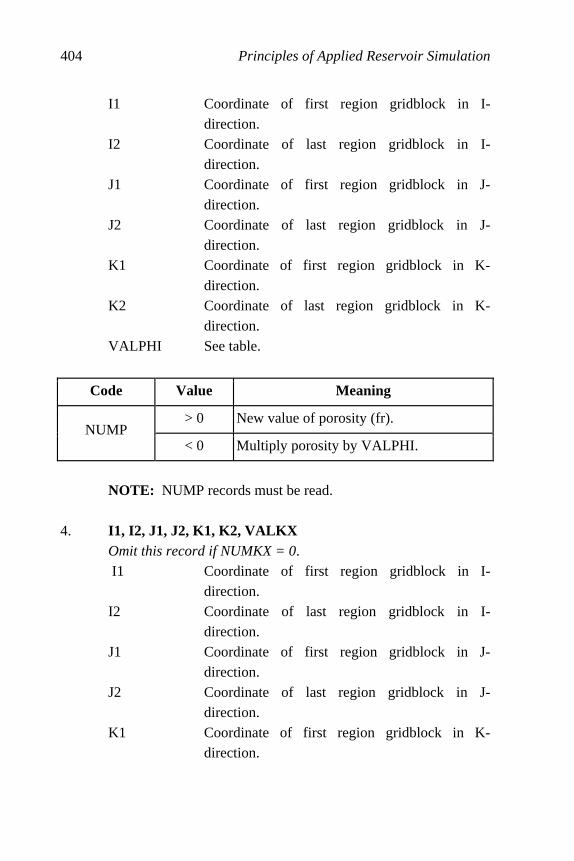
404 Principles of Applied Reservoir Simulation
I1 Coordinate of first region gridblock in I-direction.
I2 Coordinate of last region gridblock in I-direction.
J1 Coordinate of first region gridblock in J-direction.
J2 Coordinate of last region gridblock in J-direction.
K1 Coordinate of first region gridblock in K-direction.
K2 Coordinate of last region gridblock in K-direction.
VALPHI See table.
Code Value Meaning
> 0 New value of porosity (fr). NUMP
< 0 Multiply porosity by VALPHI.
NOTE: NUMP records must be read.
4. I1, I2, J1, J2, K1, K2, VALKX
Omit this record if NUMKX = 0. I1 Coordinate of first region gridblock in I-
direction. I2 Coordinate of last region gridblock in I-
direction. J1 Coordinate of first region gridblock in J-
direction. J2 Coordinate of last region gridblock in J-
direction. K1 Coordinate of first region gridblock in K-
direction.

Initialization Data 405
K2 Coordinate of last region gridblock in K-direction.
VALKX See table.
Code Value Meaning
> 0 Specify value of x-direction permeability (md). NUMKX
< 0 Multiply x-direction permeability by VALKX.
NOTE: NUMKX records must be read.
5. I1, I2, J1, J2, K1, K2, VALKY
Omit this record if NUMKY = 0. I1 Coordinate of first region gridblock in I-
direction. I2 Coordinate of last region gridblock in I-
direction. J1 Coordinate of first region gridblock in J-
direction. J2 Coordinate of last region gridblock in J-
direction. K1 Coordinate of first region gridblock in K-
direction. K2 Coordinate of last region gridblock in K-
direction. VALKY See table.
Code Value Meaning
> 0 Specify value of y-direction permeability (md). NUMKY
< 0 Multiply y-direction permeability by VALKY.
NOTE: NUMKY records must be read.

406 Principles of Applied Reservoir Simulation
6. I1, I2, J1, J2, K1, K2, VALKZ Omit this record if NUMKZ = 0. I1 Coordinate of first region gridblock in I-
direction. I2 Coordinate of last region gridblock in I-
direction. J1 Coordinate of first region gridblock in J-
direction. J2 Coordinate of last region gridblock in J-
direction. K1 Coordinate of first region gridblock in K-
direction. K2 Coordinate of last region gridblock in K-
direction. VALKZ See table.
Code Value Meaning
> 0 Specify value of z-direction permeability (md). NUMKZ
< 0 Multiply z-direction permeability by VALKZ.
NOTE: NUMKZ records must be read.
21.3 Rock Region Information
21.3.1 Definition of Rock Regions 1. Heading Up to 80 characters. 2. KR3P, NROCK, KPHIMOD
KR3P Code specifying desired relative permeability option.
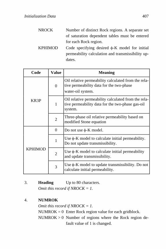
Initialization Data 407
NROCK Number of distinct Rock regions. A separate set of saturation dependent tables must be entered for each Rock region.
KPHIMOD Code specifying desired φ-K model for initial permeability calculation and transmissibility up-dates.
Code Value Meaning
0 Oil relative permeability calculated from the rela-tive permeability data for the two-phase
water-oil system.
1 Oil relative permeability calculated from the rela-tive permeability data for the two-phase gas-oil system.
KR3P
2 Three-phase oil relative permeability based on modified Stone equation
0 Do not use φ-K model.
1 Use φ-K model to calculate initial permeability. Do not update transmissibility.
2 Use φ-K model to calculate initial permeability and update transmissibility.
KPHIMOD
3 Use φ-K model to update transmissibility. Do not calculate initial permeability.
3. Heading Up to 80 characters.
Omit this record if NROCK = 1. 4. NUMROK
Omit this record if NROCK = 1. NUMROK = 0 Enter Rock region value for each gridblock. NUMROK > 0 Number of regions where the Rock region de-
fault value of 1 is changed.
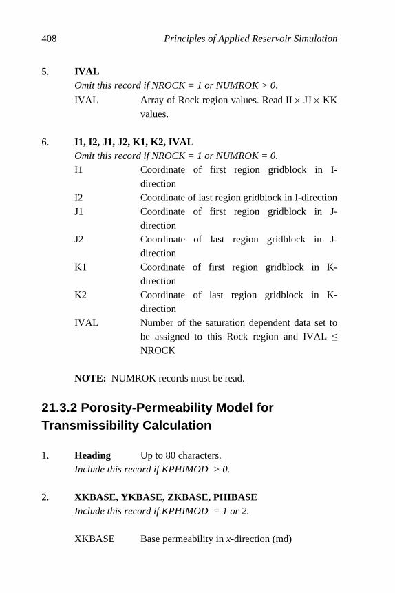
408 Principles of Applied Reservoir Simulation
5. IVAL Omit this record if NROCK = 1 or NUMROK > 0.
IVAL Array of Rock region values. Read II × JJ × KK values.
6. I1, I2, J1, J2, K1, K2, IVAL
Omit this record if NROCK = 1 or NUMROK = 0. I1 Coordinate of first region gridblock in I-
direction I2 Coordinate of last region gridblock in I-direction J1 Coordinate of first region gridblock in J-
direction J2 Coordinate of last region gridblock in J-
direction K1 Coordinate of first region gridblock in K-
direction K2 Coordinate of last region gridblock in K-
direction IVAL Number of the saturation dependent data set to
be assigned to this Rock region and IVAL ≤ NROCK
NOTE: NUMROK records must be read.
21.3.2 Porosity-Per meability Model for Transmissibility Calculation 1. Heading Up to 80 characters.
Include this record if KPHIMOD > 0. 2. XKBASE, YKBASE, ZKBASE, PHIBASE
Include this record if KPHIMOD = 1 or 2. XKBASE Base permeability in x-direction (md)
Initialization Data 409
YKBASE Base permeability in y-direction (md) ZKBASE Base permeability in z-direction (md) PHIBASE Base porosity (fr)
NOTE: The x-direction φ-K model is
( )[ ]
⎪⎭
⎪⎬⎫
⎪⎩
⎪⎨⎧
+⎟⎟⎠
⎞⎜⎜⎝
⎛
φφ
= φ−φ base2
1
2base
1base,b
b
xx eaaKK
Similar models apply to y-direction and z-direction permeabili-ties. Coefficients are defined below.
3. XKPHIA1, XKPHIB1, XKPHIA2, XKPHIB2
Include this record if KPHIMOD > 0.
XKPHIA1 Coefficient a1 for φ-K model in x-direction
XKPHIB1 Coefficient b1 for φ-K model in x-direction
XKPHIA2 Coefficient a2 for φ-K model in x-direction
XKPHIB2 Coefficient b2 for φ-K model in x-direction 4. YKPHIA1, YKPHIB1, YKPHIA2, YKPHIB2
Include this record if KPHIMOD > 0.
YKPHIA1 Coefficient a1 for φ-K model in y-direction
YKPHIB1 Coefficient b1 for φ-K model in y-direction
YKPHIA2 Coefficient a2 for φ-K model in y-direction
YKPHIB2 Coefficient b2 for φ-K model in y-direction 5. ZKPHIA1, ZKPHIB1, ZKPHIA2, ZKPHIB2
Include this record if KPHIMOD > 0.
ZKPHIA1 Coefficient a1 for φ-K model in z-direction
ZKPHIB1 Coefficient b1 for φ-K model in z-direction
ZKPHIA2 Coefficient a2 for φ-K model in z-direction
410 Principles of Applied Reservoir Simulation
ZKPHIB2 Coefficient b2 for φ-K model in z-direction
NOTE: Repeat records 1 through 5 a total of NROCK times (one set of records for each Rock Region defined in Section 21.3.1).
21.3.3 Relative Permeability and Capillary Pressure Tables 1. Heading Up to 80 characters. 2. SAT1 KROW1 KRW1 PCOW1
M
SATn KROWn KRWn PCOWn SAT Water phase saturation (fr). Set SATn = 1.0 KROW Oil relative permeability for oil-water system
(fr) KRW Water relative permeability for oil-water system
(fr) PCOW Oil-water capillary pressure (psi)
NOTE: There must be table entries for irreducible water satura-tion (Swr) and residual oil saturation (Sorw). Capillary pressure is defined as PCOW = Po - Pw where Po and Pw are the oil and wa-ter phase pressures respectively.
NOTE: Repeat records 1 and 2 a total of NROCK times (one set of records for each Rock Region defined in Section 21.3).
3. Heading Up to 80 characters. 4. SAT1 KROG1 KRG1 PCGO1
M
SATn KROGn KRGn PCGOn

Initialization Data 411
SAT Gas phase saturation (fr). Set SAT1 = 0.0 and SATn = 1.0
KROG Oil relative permeability for gas-oil system (fr) KRG Gas relative permeability for gas-oil system (fr) PCGO Gas-oil capillary pressure (psi)
NOTE: The gas-oil table assumes that irreducible water satura-tion (Swr) is present. As a matter of consistency, KROG at SAT1 = 0 must equal KROW at Swr. There must be table entries for re-sidual gas saturation (Sgr) and residual oil saturation (Sorg). Capillary pressure is defined as PCGO = Pg - Po where Po and Pg are the oil and gas phase pressures respectively. If solvent is in-cluded in the model, gas-oil capillary pressure will only be used at gridblocks that have pressures below the miscibility pressure.
NOTE: Repeat records 3 and 4 a total of NROCK times (one set
of records for each Rock Region defined in Section 21.3.1).
21.4 Modifications to Pore Volumes and Transmissibilities
1. Heading Up to 80 characters. 2. NUMPV, NUMTX, NUMTY, NUMTZ, ITCODE
NUMPV Number of regions where pore volume is changed
NUMTX Number of regions where x-direction transmis-sibility (TX) is changed
NUMTY Number of regions where y-direction transmis-sibility (TY) is changed
NUMTZ Number of regions where z-direction transmis-sibility (TZ) is changed

412 Principles of Applied Reservoir Simulation
ITCODE = 0 means do not print the modified distribu-tions = 1 means print the modified distributions
NOTE: The conventions for gridblock (I, J, K) transmissibility follow: TX(I, J, K) refers to flow between gridblocks I-1 and I. TY(I, J, K) refers to flow between gridblocks J-1 and J. TZ(I, J, K) refers to flow between gridblocks K-1 and K.
3. I1, I2, J1, J2, K1, K2, VALPV
Omit this record if NUMPV = 0. I1 Coordinate of first region gridblock in I-
direction I2 Coordinate of last region gridblock in I-direction J1 Coordinate of first region gridblock in J-
direction J2 Coordinate of last region gridblock in J-
direction K1 Coordinate of first region gridblock in K-
direction K2 Coordinate of last region gridblock in K-
direction VALPV Multiplier of pore volume for region
NOTE: NUMPV records must be read.
4. I1, I2, J1, J2, K1, K2, VALTX
Omit this record if NUMTX = 0. I1 Coordinate of first region gridblock in I-
direction I2 Coordinate of last region gridblock in I-direction J1 Coordinate of first region gridblock in J-
direction
Initialization Data 413
J2 Coordinate of last region gridblock in J-direction
K1 Coordinate of first region gridblock in K-direction
K2 Coordinate of last region gridblock in K-direction
VALTX Multiplier of x-direction transmissibility for re-gion
NOTE: NUMTX records must be read.
5. I1, I2, J1, J2, K1, K2, VALTY
Omit this record if NUMTY = 0. I1 Coordinate of first region gridblock in I-
direction I2 Coordinate of last region gridblock in I-direction J1 Coordinate of first region gridblock in J-
direction J2 Coordinate of last region gridblock in J-
direction K1 Coordinate of first region gridblock in K-
direction K2 Coordinate of last region gridblock in K-
direction VALTY Multiplier of y-direction transmissibility for re-
gion
NOTE: NUMTY records must be read.
414 Principles of Applied Reservoir Simulation
6. I1, I2, J1, J2, K1, K2, VALTZ Omit this record if NUMTZ = 0. I1 Coordinate of first region gridblock in I-
direction I2 Coordinate of last region gridblock in I-direction J1 Coordinate of first region gridblock in J-
direction J2 Coordinate of last region gridblock in J-
direction K1 Coordinate of first region gridblock in K-
direction K2 Coordinate of last region gridblock in K-
direction VALTZ Multiplier of z-direction transmissibility for re-
gion
NOTE: NUMTZ records must be read.
21.5 Reservoir Geophysical Parameters
21.5.1 Moduli and Grain Densities 1. Heading Up to 80 characters. 2. KGPMOD, KDSMOD
KGPMOD Control code for reservoir geophysical model KDSMOD Control code for dynamic to static conversion
model
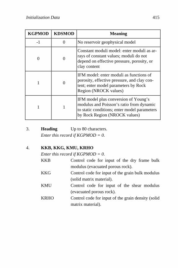
Initialization Data 415
KGPMOD KDSMOD Meaning
-1 0 No reservoir geophysical model
0 0
Constant moduli model: enter moduli as ar-rays of constant values; moduli do not depend on effective pressure, porosity, or clay content
1 0
IFM model: enter moduli as functions of porosity, effective pressure, and clay con-tent; enter model parameters by Rock Region (NROCK values)
1 1
IFM model plus conversion of Young’s modulus and Poisson’s ratio from dynamic to static conditions; enter model parameters by Rock Region (NROCK values)
3. Heading Up to 80 characters.
Enter this record if KGPMOD = 0. 4. KKB, KKG, KMU, KRHO Enter this record if KGPMOD = 0.
KKB Control code for input of the dry frame bulk modulus (evacuated porous rock).
KKG Control code for input of the grain bulk modulus (solid matrix material).
KMU Control code for input of the shear modulus (evacuated porous rock).
KRHO Control code for input of the grain density (solid matrix material).

416 Principles of Applied Reservoir Simulation
Code Value Meaning
-1 Dry frame bulk moduli are the same for all grid-blocks. Read only one value.
0 A constant value of dry frame bulk modulus is read for each layer; each layer may have a different value. Read KK values.
KKB
1 Dry frame bulk moduli are read for each gridblock. Read II × JJ × KK values.
-1 Grain bulk moduli are the same for all gridblocks. Read only one value.
0 A constant value of grain bulk modulus is read for each layer; each layer may have a different value. Read KK values.
KKG
1
Grain bulk moduli are read for each gridblock. Read II × JJ × KK values.
-1 Shear moduli are the same for all gridblocks. Read only one value.
0 A constant value of shear modulus is read for each layer; each layer may have a different value. Read KK values.
KMU
1 Shear moduli are read for each gridblock. Read II × JJ × KK values.
-1 Grain densities are the same for all gridblocks. Read only one value.
0 A constant value of grain density is read for each layer; each layer may have a different value. Read KK values.
KRHO
1 Grain densities are read for each gridblock. Read II × JJ × KK values.
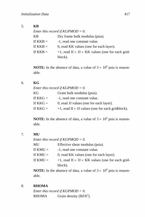
Initialization Data 417
5. KB Enter this record if KGPMOD = 0. KB Dry frame bulk modulus (psia). If KKB = -1, read one constant value. If KKB = 0, read KK values (one for each layer).
If KKB = +1, read II × JJ × KK values (one for each grid-block).
NOTE: In the absence of data, a value of 3 × 10⁶ psia is reason-
able. 6. KG
Enter this record if KGPMOD = 0. KG Grain bulk modulus (psia). If KKG = -1, read one constant value. If KKG = 0, read JJ values (one for each layer).
If KKG = +1, read II × JJ values (one for each gridblock).
NOTE: In the absence of data, a value of 3 × 10⁶ psia is reason-
able. 7. MU
Enter this record if KGPMOD = 0. MU Effective shear modulus (psia). If KMU = -1, read one constant value. If KMU = 0, read KK values (one for each layer).
If KMU = +1, read II × JJ × KK values (one for each grid-block).
NOTE: In the absence of data, a value of 3 × 10⁶ psia is reason-
able. 8. RHOMA
Enter this record if KGPMOD = 0. RHOMA Grain density (lbf/ft3).

418 Principles of Applied Reservoir Simulation
If KRHO = -1, read one constant value. If KRHO = 0, read KK values (one for each layer).
If KRHO = +1, read II × JJ × KK values (one for each grid-block).
NOTE: In the absence of data, a value of 168 lbf/ft3 (corre-sponding to 2.7 g/cm3) is reasonable.
21.5.2 IFM Model 1. Heading Up to 80 characters.
Enter this record if KGPMOD = 1. 2. AIKMA, AIKMB, AIKMC, AIKMD, AIKME, AIKMF
Enter this record if KGPMOD = 1. AIKMA Dry frame bulk modulus parameter a0 AIKMB Dry frame bulk modulus parameter a1 AIKMC Dry frame bulk modulus parameter a2 AIKMD Dry frame bulk modulus parameter a3 AIKME Dry frame bulk modulus parameter a4 AIKMF Dry frame bulk modulus parameter a5
3. EXK1, EXK2
Enter this record if KGPMOD = 1. EXK1 Dry frame bulk modulus exponent e1 EXK2 Dry frame bulk modulus exponent e2
4. AIMUA, AIMUB, AIMUC, AIMUD, AIMUE, AIMUF
Enter this record if KGPMOD = 1. AIMUA Shear modulus parameter g0 AIMUB Shear modulus parameter g1 AIMUC Shear modulus parameter g2 AIMUD Shear modulus parameter g3
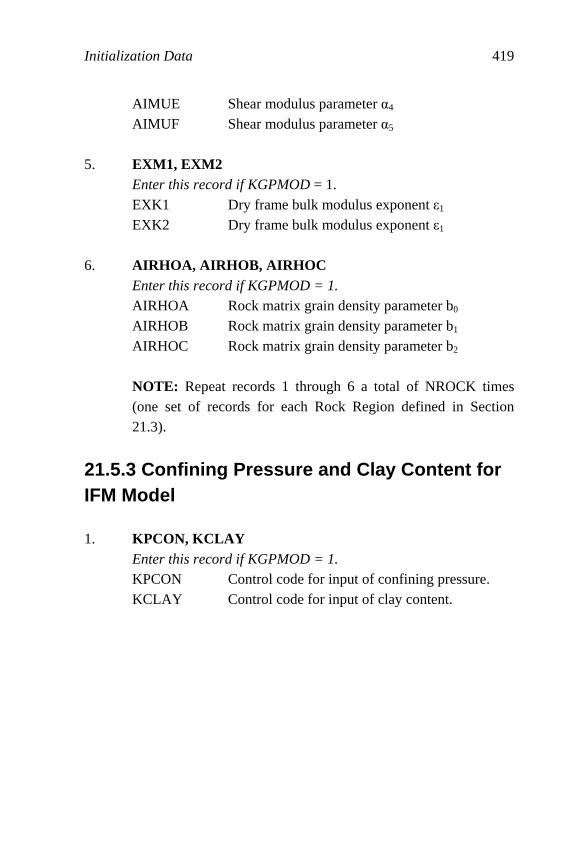
Initialization Data 419
AIMUE Shear modulus parameter g4 AIMUF Shear modulus parameter g5
5. EXM1, EXM2 Enter this record if KGPMOD = 1.
EXK1 Dry frame bulk modulus exponent i1 EXK2 Dry frame bulk modulus exponent i1
6. AIRHOA, AIRHOB, AIRHOC
Enter this record if KGPMOD = 1. AIRHOA Rock matrix grain density parameter b0 AIRHOB Rock matrix grain density parameter b1 AIRHOC Rock matrix grain density parameter b2
NOTE: Repeat records 1 through 6 a total of NROCK times (one set of records for each Rock Region defined in Section 21.3).
21.5.3 Confining Pressure and Clay Content for IFM Model 1. KPCON, KCLAY
Enter this record if KGPMOD = 1. KPCON Control code for input of confining pressure. KCLAY Control code for input of clay content.

420 Principles of Applied Reservoir Simulation
Code Value Meaning
-1 Confining pressure is the same for all gridblocks. Read only one value.
0 A constant value of confining pressure is read for each layer; each layer may have a different value. Read KK values.
1 Confining pressures are read for each gridblock. Read II × JJ × KK values.
KPCON
11 Calculate confining pressures from gridblock eleva-tions and overburden pressure gradient.
-1 Clay content is the same for all gridblocks. Read only one value.
0 A constant value of clay content is read for each layer; each layer may have a different value. Read KK values.
KCLAY
1 Clay content is read for each gridblock. Read II × JJ × KK values.
2. PCON
Enter this record if KGPMOD = 1. PCON Confining pressure (psia). If KPCON = -1, read one constant value. If KPCON = 0, read KK values (one for each layer).
If KPCON = +1, read II × JJ × KK values (one for each grid-block).
If KPCON = +11, read constant values for OBGRAD, OBDAT
OBGRAD Overburden pressure gradient (psia/ft) OBDAT Overburden datum (ft)

Initialization Data 421
NOTE: In the absence of data, values of OBGRAD = 1.0 psia/ft and OBDAT = 0.0 ft are reasonable.
3. CLAY
Enter this record if KGPMOD = 1. CLAY Clay content (volume fraction). If KCLAY = -1, read one constant value. If KCLAY = 0, read JJ values (one for each layer).
If KCLAY = +1, read II × JJ values (one for each gridblock).
NOTE: In the absence of data, a value of 0.0 is reasonable.
21.5.4 Modifications to Confining Pressure and Clay Content 1. Heading Up to 80 characters. 2. NUMCON, NUMCLA, IDCODE
NUMCON Number of regions where confining pressure (PCON) is changed.
NUMCLA Number of regions where clay content (CLAY) is changed.
IDCODE = 0 means do not print the modified distribu-tions; = 1 means print the modified distributions.
3. I1, I2, J1, J2, K1, K2, PCON
Omit this record if NUMCON = 0. I1 Coordinate of first region gridblock in I-
direction. I2 Coordinate of last region gridblock in I-
direction. J1 Coordinate of first region gridblock in J-
direction.

422 Principles of Applied Reservoir Simulation
J2 Coordinate of last region gridblock in J-direction.
K1 Coordinate of first region gridblock in K-direction.
K2 Coordinate of last region gridblock in K-direction.
PCON New value of confining pressure (psia).
NOTE: NUMCON records must be read. 4. I1, I2, J1, J2, K1, K2, CLAY
Omit this record if NUMCLA = 0. I1 Coordinate of first region gridblock in I-
direction. I2 Coordinate of last region gridblock in I-
direction. J1 Coordinate of first region gridblock in J-
direction. J2 Coordinate of last region gridblock in J-
direction. K1 Coordinate of first region gridblock in K-
direction. K2 Coordinate of last region gridblock in K-
direction. CLAY New value of clay content (volume fraction).
NOTE: NUMCLA records must be read.
21.5.5 Dynamic to Static Conversion of Young’s Modulus and Poisson’s Ratio 1. Heading Up to 80 characters.
Enter this record if KGPMOD = 1 and KDSMOD = 1.
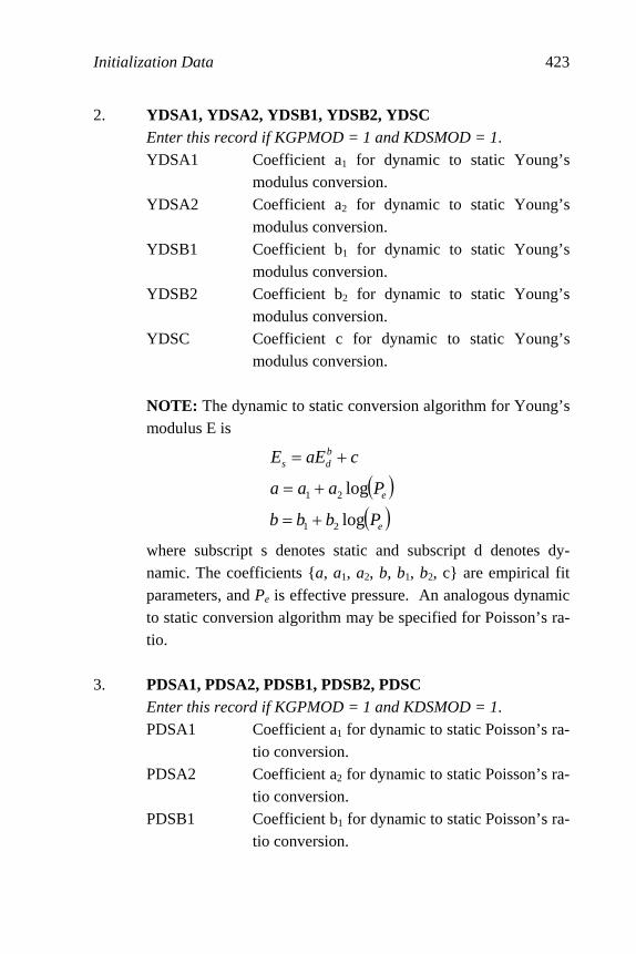
Initialization Data 423
2. YDSA1, YDSA2, YDSB1, YDSB2, YDSC Enter this record if KGPMOD = 1 and KDSMOD = 1. YDSA1 Coefficient a1 for dynamic to static Young’s
modulus conversion. YDSA2 Coefficient a2 for dynamic to static Young’s
modulus conversion. YDSB1 Coefficient b1 for dynamic to static Young’s
modulus conversion. YDSB2 Coefficient b2 for dynamic to static Young’s
modulus conversion. YDSC Coefficient c for dynamic to static Young’s
modulus conversion.
NOTE: The dynamic to static conversion algorithm for Young’s modulus E is
( )( )e
e
bds
Pbbb
Paaa
caEE
log
log
21
21
+=
+=
+=
where subscript s denotes static and subscript d denotes dy-namic. The coefficients {a, a1, a2, b, b1, b2, c} are empirical fit parameters, and Pe is effective pressure. An analogous dynamic to static conversion algorithm may be specified for Poisson’s ra-tio.
3. PDSA1, PDSA2, PDSB1, PDSB2, PDSC Enter this record if KGPMOD = 1 and KDSMOD = 1. PDSA1 Coefficient a1 for dynamic to static Poisson’s ra-
tio conversion. PDSA2 Coefficient a2 for dynamic to static Poisson’s ra-
tio conversion. PDSB1 Coefficient b1 for dynamic to static Poisson’s ra-
tio conversion.

424 Principles of Applied Reservoir Simulation
PDSB2 Coefficient b2 for dynamic to static Poisson’s ra-tio conversion.
PDSC Coefficient c for dynamic to static Poisson’s ra-tio conversion.
NOTE: Repeat records 1 through 3 a total of NROCK times (one set of records for each Rock Region defined in Section 21.3).
21.6 Fluid PVT Tables 1. Heading Up to 80 characters. 2. PBO, VOSLP, BOSLP, BWSLP, PMAX
PBO Initial reservoir oil bubble point pressure (psia). If no oil or natural gas exist, set PBO = 14.7 psia.
VOSLP Slope of the oil viscosity versus pressure curve for undersaturated oil, i.e. for pressures above PBO. The slope (〉µo/〉Po) should be in cp/psia.
BOSLP Slope of the oil formation volume factor versus pressure curve for undersaturated oil. The slope (〉Bo/〉Po) should be in RB/STB/psia and should be negative or zero.
BWSLP Slope of the water formation volume factor ver-sus pressure curve for undersaturated water, i.e. for pressures above PBO. The slope (〉Bw/〉Po) should be in RB/STB/psia and should be nega-tive or zero.
PMAX Maximum pressure entry for all PVT tables (psia).
NOTE: VOSLP, BOSLP and BWSLP are used only for under-saturated oil and water. The slope (〉Rso/〉Po) of the solution

Initialization Data 425
natural gas-oil ratio versus pressure curve for undersaturated oil is assumed to be zero.
3. Heading Up to 80 characters; oil table follows. 4. P1 MUO1 BO1 RSO1
M
PMAX MUO(PMAX) BO(PMAX) RSO(PMAX) P Pressure (psia). Pressures must be in ascending
order from P1 (normally 14.7 psia) to PMAX. The last table entry must be PMAX.
MUO Oil viscosity (cp). BO Oil formation volume factor (RB/STB). RSO Solution natural gas-oil ratio (SCF/STB).
NOTE: Oil properties must be entered as saturated data over the entire pressure range. Saturated oil data is required because of the bubble point pressure tracking algorithm.
5. Heading Up to 80 characters; water table follows. 6. P1 MUW1 BW1 RSW1
M
PMAX MUW(PMAX) BW(PMAX) RSW(PMAX) P Pressure (psia). Pressures must be in ascending
order from P1 (normally 14.7 psia) to PMAX. The last table entry must be PMAX.
MUW Water viscosity (cp). BW Water formation volume factor (RB/STB). RSW Solution natural gas-water ratio (SCF/STB).
Water properties must be entered as saturated data over the entire pressure range if RSW in nonzero.

426 Principles of Applied Reservoir Simulation
NOTE: It is usually assumed in black oil simulations that the solubility of gas in water can be neglected. In this case, set RSW = 0.0 for all pressures. IFLO includes gas solubility in the water phase to account for CO2 solubility in water, gas production from geopressured aquifers, or any other case where gas solubil-ity in water can be significant.
7. Heading Up to 80 characters. 8. KGCOR
Code Value Meaning
0
Read gas and rock properties table.
KGCOR 1
Activate gas correlation option and read rock compressibility versus pressure table.
9. Heading Up to 80 characters; gas table follows.
Omit this record if KGCOR = 1. 10. P1 MUG1 BG1 PSI1 CR1
M
PMAX MUG(PMAX) BG(PMAX) PSI(PMAX) CR(PMAX) Omit this record if KGCOR = 1.
P Pressure (psia). Pressures must be in ascending
order from P1 (normally 14.7 psia) to PMAX. The last table entry must be PMAX.
MUG Natural gas viscosity (cp). BG Natural gas formation volume factor
(RCF/SCF). PSI Real gas pseudo-pressure (psia2/cp). CR Rock compressibility (1/psia).
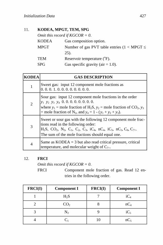
Initialization Data 427
11. KODEA, MPGT, TEM, SPG Omit this record if KGCOR = 0. KODEA Gas composition option.
MPGT Number of gas PVT table entries (1 < MPGT ≤ 25).
TEM Reservoir temperature (oF). SPG Gas specific gravity (air = 1.0).
KODEA GAS DESCRIPTION
1 Sweet gas: input 12 component mole fractions as 0. 0. 0. 1. 0. 0. 0. 0. 0. 0. 0. 0.
2
Sour gas: input 12 component mole fractions in the order y1 y2 y3 y4 0. 0. 0. 0. 0. 0. 0. 0. where y1 = mole fraction of H2S, y2 = mole fraction of CO2, y3 = mole fraction of N2, and y4 = 1 - (y1 + y2 + y3).
3
Sweet or sour gas with the following 12 component mole frac-tions read in the following order: H2S, CO2, N2, C1, C2, C3, iC4, nC4, iC5, nC5, C6, C7+. The sum of the mole fractions should equal one.
4 Same as KODEA = 3 but also read critical pressure, critical temperature, and molecular weight of C7+.
12. FRCI
Omit this record if KGCOR = 0. FRCI Component mole fraction of gas. Read 12 en-
tries in the following order.
FRCI(I) Component I FRCI(I) Component I
1 H2S 7 iC4
2 CO2 8 nC4
3 N2 9 iC5
4 C1 10 nC5

428 Principles of Applied Reservoir Simulation
FRCI(I) Component I FRCI(I) Component I
5 C2 11 C6
6 C3 12 C7+
13. PRSCI, TEMCI, RMWTI
Omit this record if KGCOR = 0 or if KODEA ≠ 4.
PRSCI Critical pressure (psia). TEMCI Critical temperature (oR). RMWTI Molecular weight.
14. Heading Up to 80 characters.
Omit this record if KGCOR = 0. NOTE: Rock compressibility table follows. 15. P1 CR1
M
PMAX CR(PMAX) Omit this record if KGCOR = 0.
Number of Records Variable Meaning
Option 1. Constant rock compressibility
PMAX Maximum table pressure (psia) from record 4. Enter one record.
CR Rock compressibility (1/psia)
Option 2. Pressure-dependent rock compressibility
P
Pressure (psia). Pressures must be in ascending order from P1 (normally 14.7 psia) to PMAX. The last table entry must be PMAX.
Enter MPGT
records.
CR Rock compressibility (1/psia)
Initialization Data 429
16. Heading Up to 80 characters. 17. RHOSCO, RHOSCW, RHOSCG
RHOSCO Stock tank oil density (lbm/cu ft). RHOSCW Stock tank water density (lbm/cu ft). RHOSCG Gas density at standard conditions (lbm/cu ft). If
no natural gas exists, set RHOSCG = 0.
NOTE: At stock tank conditions (14.7 psia and 60 degrees F for oilfield units) pure water has a density of 62.4 lbm/cu ft and air has a density of 0.0765 lbm/cu ft.
21.7 Miscible Solvent Data 1. Heading Up to 80 characters. 2. NSLUGS, NSREAD
NSLUGS Number of solvents. NSREAD Number of solvent PVT tables to be read (up to
4). NSREAD must be equal to or greater than NSLUGS.
NOTE: NSREAD is provided as a convenience. PVT data for one to four solvents may be left in the input data set for an oil-water-natural gas run by setting NSREAD = 1 to 4 and NSLUGS = 0.
If NSREAD = 0, omit the data in the remainder of this section and proceed to Section 21.8. 3. Heading Up to 80 characters. 4. PBO1, VO1OPE, BO1OPE

430 Principles of Applied Reservoir Simulation
PBO1 Initial base solvent-oil bubble point pressure (psia).
VO1OPE Undersaturated slope of oil viscosity (cp/psi). BO1OPE Undersaturated slope of oil formation volume
factor (RB/STB/psi). 5. Heading Up to 80 characters. 6. PBW1, VW1OPE, BW1OPE
PBW1 Initial base solvent-water bubble point pressure (psia).
VW1OPE Undersaturated slope of water viscosity (cp/psi). BW1OPE Undersaturated slope of water formation volume
factor (RB/STB/psi). 7. Heading Up to 80 characters. 8. PMISC, FPMISC, SOMIN, REDK, BETA, SORM, VSMISC
PMISC Miscibility pressure (psia). FPMISC Fraction of PMISC (fr) for calculating multi-
contact miscibility pressure PMCM (psia). PMISC and PMCM are related by PMCM =
FPMISC × PMISC. SOMIN Minimum oil saturation for solid precipitation
(fr). SOMIN > 0 only if SORM = 0. REDK Relative permeability reduction factor for solid
precipitation (fr). BETA Parameter for water blocking function. SORM Miscible region residual oil saturation (fr).
SORM > 0 only if SOMIN = 0. VSMISC Total solvent volume fraction required to obtain
full miscibility (fr).

Initialization Data 431
Code Value Meaning
0 No solid precipitation. SOMIN
> 0 Allow solid precipitation.
< 0 No water blocking. BETA
≥ 0 Water blocking on.
NOTE: If the automatic timestep control is on, saturation con-vergence requires that SOMIN < DSMAX (Section 21.9).
9. Heading Up to 80 characters. 10. OM1, OM2
OM1 Mixing parameter の1 for natural gas-solvent miscibility.
OM2 Mixing parameter の2 for oil-gas-solvent misci-bility.
NOTE: Only OM1 is used if the gridblock pressure P < PMCM. Only OM2 is used if P > PMISC. Both OM1 and OM2 are used if P is in the multicontact miscibility pressure range PMCM < P < PMISC.
11. Heading Up to 80 characters. 12. RHOSC1, RHOSC2, RHOSC3, RHOSC4
RHOSC1 Stock tank density of base solvent (lbm/cu ft). RHOSC2 Stock tank density of solvent 2 (lbm/cu ft). RHOSC3 Stock tank density of solvent 3 (lbm/cu ft). RHOSC4 Stock tank density of solvent 4 (lbm/cu ft).
13. Heading Up to 80 characters. 14. Heading Up to 80 characters.
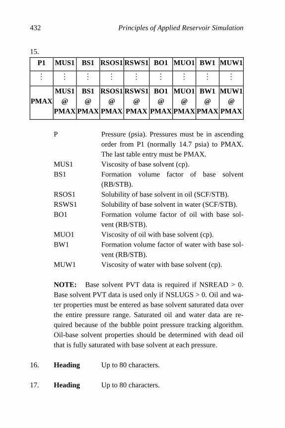
432 Principles of Applied Reservoir Simulation
15.
P1 MUS1 BS1 RSOS1 RSWS1 BO1 MUO1 BW1 MUW1
M M M M M M M M M
PMAX MUS1
@ PMAX
BS1 @
PMAX
RSOS1@
PMAX
RSWS1@
PMAX
BO1 @
PMAX
MUO1@
PMAX
BW1@
PMAX
MUW1@
PMAX
P Pressure (psia). Pressures must be in ascending
order from P1 (normally 14.7 psia) to PMAX. The last table entry must be PMAX.
MUS1 Viscosity of base solvent (cp). BS1 Formation volume factor of base solvent
(RB/STB). RSOS1 Solubility of base solvent in oil (SCF/STB). RSWS1 Solubility of base solvent in water (SCF/STB). BO1 Formation volume factor of oil with base sol-
vent (RB/STB). MUO1 Viscosity of oil with base solvent (cp). BW1 Formation volume factor of water with base sol-
vent (RB/STB). MUW1 Viscosity of water with base solvent (cp).
NOTE: Base solvent PVT data is required if NSREAD > 0. Base solvent PVT data is used only if NSLUGS > 0. Oil and wa-ter properties must be entered as base solvent saturated data over the entire pressure range. Saturated oil and water data are re-quired because of the bubble point pressure tracking algorithm. Oil-base solvent properties should be determined with dead oil that is fully saturated with base solvent at each pressure.
16. Heading Up to 80 characters. 17. Heading Up to 80 characters.
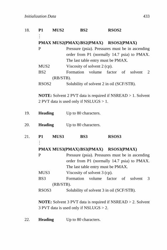
Initialization Data 433
18. P1 MUS2 BS2 RSOS2
M
PMAX MUS2(PMAX) BS2(PMAX) RSOS2(PMAX) P Pressure (psia). Pressures must be in ascending
order from P1 (normally 14.7 psia) to PMAX. The last table entry must be PMAX.
MUS2 Viscosity of solvent 2 (cp). BS2 Formation volume factor of solvent 2
(RB/STB). RSOS2 Solubility of solvent 2 in oil (SCF/STB).
NOTE: Solvent 2 PVT data is required if NSREAD > 1. Solvent 2 PVT data is used only if NSLUGS > 1.
19. Heading Up to 80 characters. 20. Heading Up to 80 characters. 21. P1 MUS3 BS3 RSOS3
M
PMAX MUS3(PMAX) BS3(PMAX) RSOS3(PMAX) P Pressure (psia). Pressures must be in ascending
order from P1 (normally 14.7 psia) to PMAX. The last table entry must be PMAX.
MUS3 Viscosity of solvent 3 (cp). BS3 Formation volume factor of solvent 3
(RB/STB). RSOS3 Solubility of solvent 3 in oil (SCF/STB).
NOTE: Solvent 3 PVT data is required if NSREAD > 2. Solvent 3 PVT data is used only if NSLUGS > 2.
22. Heading Up to 80 characters.

434 Principles of Applied Reservoir Simulation
23. Heading Up to 80 characters. 24. P1 MUS4 BS4 RSOS4
M
PMAX MUS4(PMAX) BS4(PMAX) RSOS4(PMAX) P Pressure (psia). Pressures must be in ascending
order from P1 (normally 14.7 psia) to PMAX. The last table entry must be PMAX.
MUS4 Viscosity of solvent 4 (cp). BS4 Formation volume factor of solvent 4
(RB/STB). RSOS4 Solubility of solvent 4 in oil (SCF/STB).
NOTE: Solvent 4 PVT data is required if NSREAD > 3. Solvent 4 PVT data is used only if NSLUGS > 3.
25. Heading Up to 80 characters. 26. NOMOB, MOBCTL, SCI
NOMOB Number of entries in the mobility control table. MOBCTL Mobility control switch. SCI Surfactant concentration index. SCI multiplies
the mobility reduction values FRCO2 defined below.
Code Value Meaning
0 No mobility control. MOBCTL
1 Apply mobility control.
27. Heading Up to 80 characters.
Omit this record if MOBCTL = 0.

Initialization Data 435
28. NSC, FRCO2 Omit this record if MOBCTL = 0. NSC Normalized surfactant concentration (fr). FRCO2 Reduction of base solvent mobility (fr).
NOTE: NOMOB records must be read.
21.8 Pressure and Saturation Initialization
1. Heading Up to 80 characters.
2. KPI, KSI KPI Pressure initialization code. KSI Saturation initialization code.
CodeValues
KPI KSI Meaning
0 0
Equilibrium pressure and saturation initialization. Enter pressures and depths at the OWC and GOC. This option assumes no solvent present at initialization. Saturations are calculated from capillary pressures.
1 Specify pressure throughout grid. Read II × JJ × KK val-ues of P.
1 Specify constant initial oil, water and gas saturations; specify constant initial solvent volume fractions.
2 Specify variable saturations throughout grid. Read II × JJ × KK values of SO, SW, and solvent volume fractions. IFLO sets SG = 1 − SO − SW internally.
0 3 Gravity segregated oil, water and gas saturations. This option assumes no solvent present at initialization.
NOTE: Option {KPI = 1, KSI = 2} may be used to prepare a re-start data file.

436 Principles of Applied Reservoir Simulation
3. WOC, PWOC, GOC, PGOC Enter this record if KPI = 0. WOC Depth to the water-oil contact (ft below datum). PWOC Pressure at the water-oil contact (psia). GOC Depth to the gas-oil contact (ft below datum). PGOC Pressure at the gas-oil contact (psia).
NOTE: Repeat this record a total of NROCK times: one record for each Rock region defined in Section 21.3.
4. PO
Enter this record if KPI = 1.
PO Oil phase pressure (psia). Read II × JJ × KK values.
5. SOI, SWI, SGI, VS1I, VS2I, VS3I, VS4I
Enter this record if KSI = 1. SOI Initial oil saturation (fr). SWI Initial water saturation (fr). SGI Initial gas saturation (fr). Omit the following values if NSLUGS = 0. VS1I Initial base solvent volume fraction in the gase-
ous phase (fr). Enter this value if NSLUGS ≥ 1. VS2I Initial solvent 2 volume fraction in the gaseous
phase (fr). Enter this value if NSLUGS ≥ 2. VS3I Initial solvent 3 volume fraction in the gaseous
phase (fr). Enter this value if NSLUGS ≥ 3. VS4I Initial solvent 4 volume fraction in the gaseous
phase (fr). Enter this value if NSLUGS ≥ 4.
NOTE: The sum of the saturations must satisfy SOI + SWI + SGI = 1 and the sum of the volume fractions must satisfy the constraint VGG + VS1 + VS2 + VS3 + VS4 = 1.0 where VGG is the fraction of natural gas in the gaseous phase.
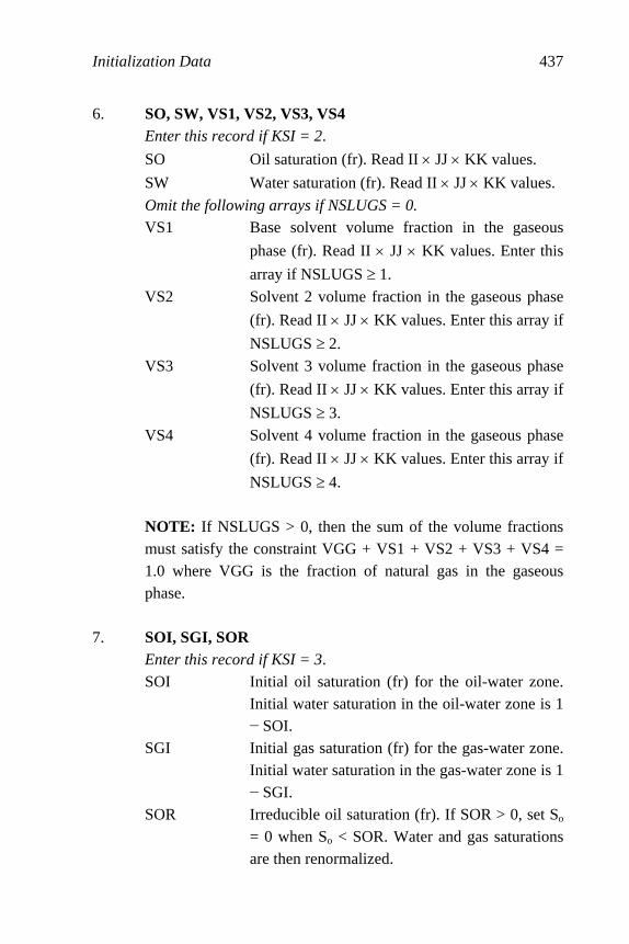
Initialization Data 437
6. SO, SW, VS1, VS2, VS3, VS4 Enter this record if KSI = 2.
SO Oil saturation (fr). Read II × JJ × KK values.
SW Water saturation (fr). Read II × JJ × KK values.
Omit the following arrays if NSLUGS = 0. VS1 Base solvent volume fraction in the gaseous
phase (fr). Read II × JJ × KK values. Enter this
array if NSLUGS ≥ 1.
VS2 Solvent 2 volume fraction in the gaseous phase
(fr). Read II × JJ × KK values. Enter this array if
NSLUGS ≥ 2. VS3 Solvent 3 volume fraction in the gaseous phase
(fr). Read II × JJ × KK values. Enter this array if
NSLUGS ≥ 3. VS4 Solvent 4 volume fraction in the gaseous phase
(fr). Read II × JJ × KK values. Enter this array if
NSLUGS ≥ 4.
NOTE: If NSLUGS > 0, then the sum of the volume fractions must satisfy the constraint VGG + VS1 + VS2 + VS3 + VS4 = 1.0 where VGG is the fraction of natural gas in the gaseous phase.
7. SOI, SGI, SOR
Enter this record if KSI = 3. SOI Initial oil saturation (fr) for the oil-water zone.
Initial water saturation in the oil-water zone is 1 − SOI.
SGI Initial gas saturation (fr) for the gas-water zone. Initial water saturation in the gas-water zone is 1 − SGI.
SOR Irreducible oil saturation (fr). If SOR > 0, set So = 0 when So < SOR. Water and gas saturations are then renormalized.

438 Principles of Applied Reservoir Simulation
NOTE: Repeat this record a total of NROCK times: one record for each Rock region defined in Section 21.3.
21.9 Run Control Parameters
1. Heading Up to 80 characters.
2. KSW1, KSW2, KSW3, KSW4 KSW1 Control code for printing material balance in-
formation. Information includes the gridblock location with the largest component material balance error, the magnitude of the error, and the elapsed time.
KSW2 Control code for graphical image orientation. KSW3 Control code for printing the number of itera-
tions required for convergence of the iterative solution techniques (SSOR, LSOR, ORTHOMIN).
KSW4 Control code for printing timestep summary to terminal.
Code Code Value Meaning
0 Do not print the information KSW1
1 Print the information to file ITEMP.MBE
0 Image aligned with grid KSW2
1 Image inverted relative to y-axis
0 Do not print the information KSW3
1 Print the information to file ITEMP.MBE
0 Print summary at each timestep KSW4
1 Print summary at FTIO times (Section 22.1)

Initialization Data 439
3. Heading Up to 80 characters. 4. NMAX, FACT1, FACT2, TMAX, WORMAX, GORMAX,
PAMIN, PAMAX NMAX Maximum number of timesteps per simulation
run. FACT1 Factor for increasing timestep size using auto-
matic timestep control. FACT1 = 1.0 for fixed timestep size. A common value for FACT1 is 1.25.
FACT2 Factor for decreasing timestep size using auto-matic timestep control. FACT2 = 1.0 for fixed timestep size. A common value for FACT2 is 0.5.
TMAX Maximum elapsed time to be simulated (days); the run will be terminated when the time ex-ceeds TMAX.
WORMAX Maximum allowed water-oil ratio for a produc-ing oil well (STB/STB).
GORMAX Maximum allowed gas-oil ratio for a producing oil well (SCF/STB).
PAMIN Minimum field average pressure (psia). PAMAX Maximum field average pressure (psia).
NOTE: The run will be terminated if producing WOR > WORMAX or producing GOR > GORMAX. GORMAX is the total natural gas plus solvent-oil ratio. PAMIN and PAMAX should be within the range of pressures covered by the fluid PVT tables discussed in Section 21.6. The run will be terminated when the pore volume weighted average reservoir pressure Pavg < PAMIN or Pavg > PAMAX. Each of the controls {WORMAX, GORMAX, PAMIN, PAMAX} will be ignored if it is set to zero.
5. Heading Up to 80 characters.

440 Principles of Applied Reservoir Simulation
6. KSOL, MITR, OMEGA, TOL, NCYCLE, DSMAX, DPMAX, ITMAX, RTOL, NERR KSOL Solution method code. MITR For KSOL = 1 or 2: maximum number of SOR
iterations for convergence with a typical value of 100. For KSOL = 4: maximum number of conjugate gradient iterations for convergence with a typical value of 50.
OMEGA For KSOL =1 or 2: initial SOR acceleration pa-rameter. Initial value of OMEGA should be between 1.0 and 2.0. A typical initial value is 1.2. The model will attempt to optimize OMEGA if NCYCLE ≠ 0.
TOL For KSOL = 1 or 2: maximum acceptable SOR pressure convergence tolerance with a typical value of 0.001 psia. For KSOL = 4: pressure convergence tolerance with a typical value of 0.001 psia to 0.0001 psia.
NCYCLE For KSOL = 1 or 2: number of SOR iteration cycles for determining when to change (opti-mize) OMEGA. A typical value is 12. If NCYCLE = 0, the initial value of OMEGA will be used for the entire run.
DSMAX Maximum saturation change (fraction) allowed per timestep. The timestep size DT will be re-duced by FACT2 if the saturation change of any phase or any component in any gridblock ex-ceeds DSMAX and DT > DTMIN (the user-specified minimum timestep size defined in Sec-tion 22.1). If the resulting step size is less than DTMIN, the timestep will be repeated with DT = DTMIN. A typical value of DSMAX is 0.05.

Initialization Data 441
DPMAX Maximum pressure change (psia) allowed per timestep. The timestep size will be reduced by FACT2 if the pressure change in any gridblock exceeds DPMAX and DT > DTMIN. If the re-sulting step size is less than DTMIN, the timestep will be repeated with DT = DTMIN. A typical value of DPMAX is 100 psia.
ITMAX Maximum number of Newton-Raphson itera-tions per timestep for convergence. A typical value is 5.
RTOL Maximum allowed residual for Newton-Raphson convergence. A typical value is 0.001. ITMAX overrides RTOL if RTOL is not reached.
NERR Code for controlling material balance error technique. NERR = 1 is recommended.
Code Value Meaning
1 SSOR: iterative, slice (planar) successive over-relaxation method for 2-D and 3-D models.
2 LSOR: iterative, line successive over-relaxation method for 0-D, 1-D, 2-D and 3-D models.
3 D4: direct solution method for 1-D, 2-D and moder-ate sized 3-D models.
KSOL
4
ORTHOMIN: iterative, preconditioned conjugate gradient algorithm for large 2-D and 3-D models.
0 Material balance error control technique is off. NERR
1 Material balance error control technique is on.
7. Heading Up to 80 characters. 8. WEIGHT
WEIGHT Fluid property weighting factor.
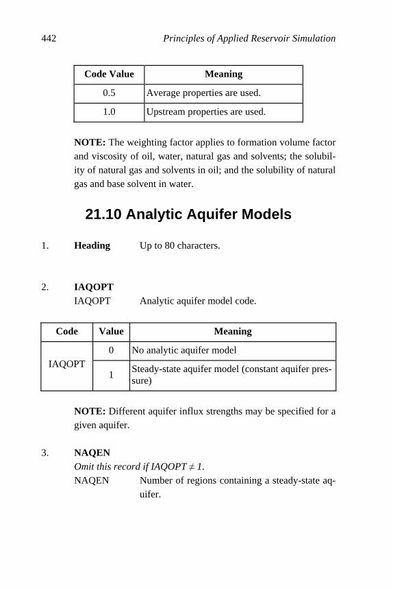
442 Principles of Applied Reservoir Simulation
Code Value Meaning
0.5 Average properties are used.
1.0 Upstream properties are used.
NOTE: The weighting factor applies to formation volume factor and viscosity of oil, water, natural gas and solvents; the solubil-ity of natural gas and solvents in oil; and the solubility of natural gas and base solvent in water.
21.10 Analytic Aquifer Models 1. Heading Up to 80 characters. 2. IAQOPT
IAQOPT Analytic aquifer model code.
Code Value Meaning
0 No analytic aquifer model IAQOPT
1 Steady-state aquifer model (constant aquifer pres-sure)
NOTE: Different aquifer influx strengths may be specified for a given aquifer.
3. NAQEN
Omit this record if IAQOPT ≠ 1. NAQEN Number of regions containing a steady-state aq-
uifer.

Initialization Data 443
4. I1, I2, J1, J2, K1, K2, SSAQ Omit this record if IAQOPT ≠1. I1 Coordinate of first region gridblock in I-
direction. I2 Coordinate of last region gridblock in I-
direction. J1 Coordinate of first region gridblock in J-
direction. J2 Coordinate of last region gridblock in J-
direction. K1 Coordinate of first region gridblock in K-
direction. K2 Coordinate of last region gridblock in K-
direction. SSAQ Steady-state aquifer strength (SCF/day/psia).
NOTE: NAQEN records must be read.
21.11 Coal Gas Model
1. Heading Up to 80 characters. 2. ICGOPT
ICGOPT Coal gas model code.
Code Value Meaning
0 No coal gas model ICGOPT
1 Coal gas model with diffusive desorption
3. NCGREG
Omit this record if ICQOPT ≠ 1. NCGREG Number of regions containing a coalbed.
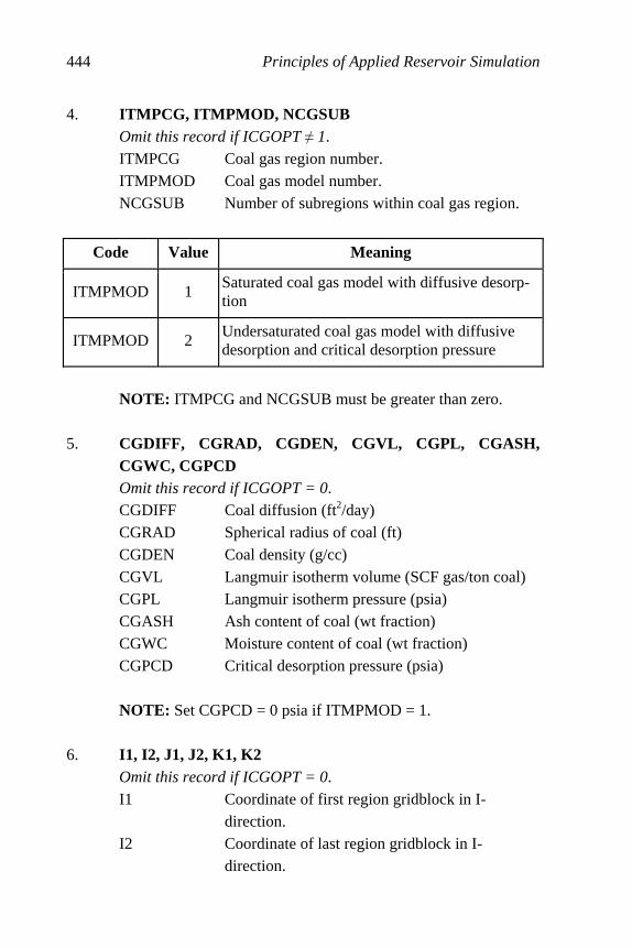
444 Principles of Applied Reservoir Simulation
4. ITMPCG, ITMPMOD, NCGSUB Omit this record if ICGOPT ≠ 1. ITMPCG Coal gas region number. ITMPMOD Coal gas model number. NCGSUB Number of subregions within coal gas region.
Code Value Meaning
ITMPMOD 1 Saturated coal gas model with diffusive desorp-tion
ITMPMOD 2 Undersaturated coal gas model with diffusive desorption and critical desorption pressure
NOTE: ITMPCG and NCGSUB must be greater than zero.
5. CGDIFF, CGRAD, CGDEN, CGVL, CGPL, CGASH,
CGWC, CGPCD Omit this record if ICGOPT = 0. CGDIFF Coal diffusion (ft2/day) CGRAD Spherical radius of coal (ft) CGDEN Coal density (g/cc) CGVL Langmuir isotherm volume (SCF gas/ton coal) CGPL Langmuir isotherm pressure (psia) CGASH Ash content of coal (wt fraction) CGWC Moisture content of coal (wt fraction) CGPCD Critical desorption pressure (psia)
NOTE: Set CGPCD = 0 psia if ITMPMOD = 1.
6. I1, I2, J1, J2, K1, K2
Omit this record if ICGOPT = 0. I1 Coordinate of first region gridblock in I-
direction. I2 Coordinate of last region gridblock in I-
direction.

Initialization Data 445
J1 Coordinate of first region gridblock in J-direction.
J2 Coordinate of last region gridblock in J-direction.
K1 Coordinate of first region gridblock in K-direction.
K2 Coordinate of last region gridblock in K-direction.
NOTE: NCGSUB records must be read.
NOTE: Records 4 and 5 should be repeated NCGREG times.

446
Chapter 22
Recurrent Data
Recurrent data records are read periodically during the course of the simulation run. These data include the location and specification of wells in the model, changes in well completions and field operations over time, a schedule of well rate or pressure performance over time (or both), timestep control information for advancing the simulation through time, and controls on the type and frequency of printout information provided by the simulator. 1. Major Heading Up to 80 characters.
NOTE: This record signifies the start of the recurrent data section.
22.1 Timestep and Output Control 1. Heading Up to 80 characters. 2. IWREAD, IOMETH, IWLREP, ISUMRY
IWREAD Controls input of well information. IOMETH Controls scheduling of well input and array print
controls. IWLREP Controls output of well report.
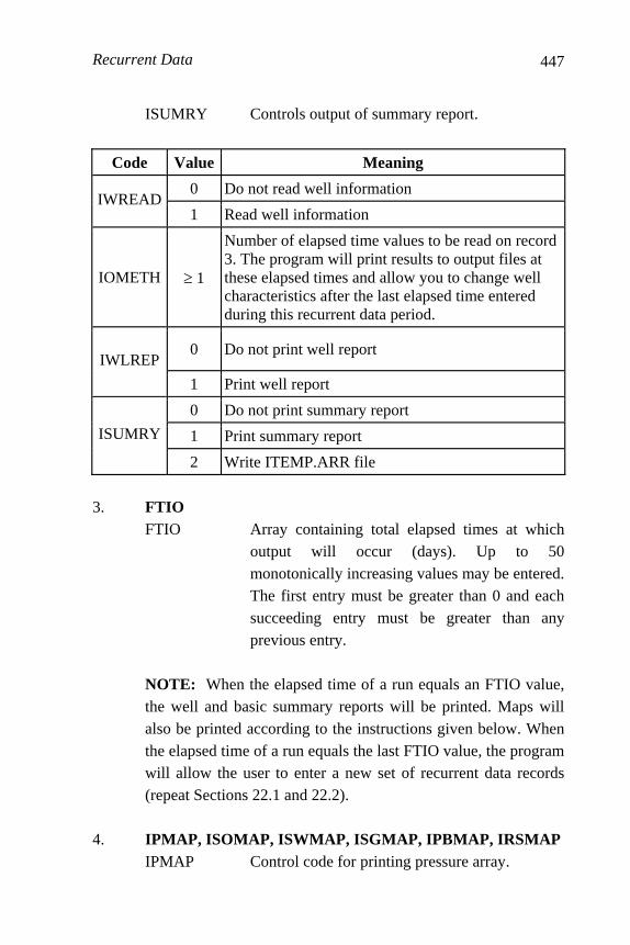
Recurrent Data
447
ISUMRY Controls output of summary report.
Code Value Meaning
0 Do not read well information IWREAD
1 Read well information
IOMETH ≥ 1
Number of elapsed time values to be read on record 3. The program will print results to output files at these elapsed times and allow you to change well characteristics after the last elapsed time entered during this recurrent data period.
0 Do not print well report IWLREP
1 Print well report
0 Do not print summary report
1 Print summary report ISUMRY
2 Write ITEMP.ARR file
3. FTIO
FTIO Array containing total elapsed times at which output will occur (days). Up to 50 monotonically increasing values may be entered. The first entry must be greater than 0 and each succeeding entry must be greater than any previous entry.
NOTE: When the elapsed time of a run equals an FTIO value, the well and basic summary reports will be printed. Maps will also be printed according to the instructions given below. When the elapsed time of a run equals the last FTIO value, the program will allow the user to enter a new set of recurrent data records (repeat Sections 22.1 and 22.2).
4. IPMAP, ISOMAP, ISWMAP, ISGMAP, IPBMAP, IRSMAP
IPMAP Control code for printing pressure array.
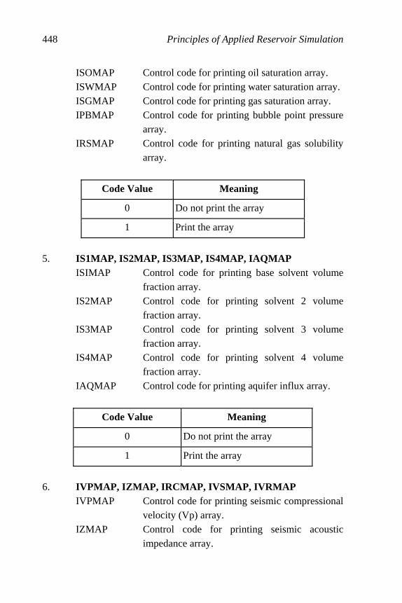
Principles of Applied Reservoir Simulation
448
ISOMAP Control code for printing oil saturation array. ISWMAP Control code for printing water saturation array. ISGMAP Control code for printing gas saturation array. IPBMAP Control code for printing bubble point pressure
array. IRSMAP Control code for printing natural gas solubility
array.
Code Value Meaning
0 Do not print the array
1 Print the array
5. IS1MAP, IS2MAP, IS3MAP, IS4MAP, IAQMAP
ISIMAP Control code for printing base solvent volume fraction array.
IS2MAP Control code for printing solvent 2 volume fraction array.
IS3MAP Control code for printing solvent 3 volume fraction array.
IS4MAP Control code for printing solvent 4 volume fraction array.
IAQMAP Control code for printing aquifer influx array.
Code Value Meaning
0 Do not print the array
1 Print the array
6. IVPMAP, IZMAP, IRCMAP, IVSMAP, IVRMAP
IVPMAP Control code for printing seismic compressional velocity (Vp) array.
IZMAP Control code for printing seismic acoustic impedance array.
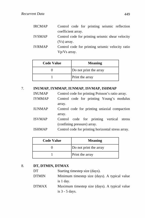
Recurrent Data
449
IRCMAP Control code for printing seismic reflection coefficient array.
IVSMAP Control code for printing seismic shear velocity (Vs) array.
IVRMAP Control code for printing seismic velocity ratio Vp/Vs array.
Code Value Meaning
0 Do not print the array
1 Print the array
7. INUMAP, IYMMAP, IUNMAP, ISVMAP, ISHMAP
INUMAP Control code for printing Poisson’s ratio array. IYMMAP Control code for printing Young’s modulus
array. IUNMAP Control code for printing uniaxial compaction
array. ISVMAP Control code for printing vertical stress
(confining pressure) array. ISHMAP Control code for printing horizontal stress array.
Code Value Meaning
0 Do not print the array
1 Print the array
8. DT, DTMIN, DTMAX
DT Starting timestep size (days). DTMIN Minimum timestep size (days). A typical value
is 1 day. DTMAX Maximum timestep size (days). A typical value
is 3 - 5 days.

Principles of Applied Reservoir Simulation
450
22.2 Well Information Omit this section if IWREAD = 0. 1. Heading Up to 80 characters 2. NWELLN, NWELLO, KSIS
NWELLN Number of new wells for which complete well information is entered
NWELLO Number of previously defined wells for which new rates and/or rate controls are entered
KSIS Control code for surfactant-water injection
Code Value Meaning
0 Do not read new well information NWELLN
≥1 Read new well information
0 Do not change data for previously defined wells NWELLO
≥1 Change data for previously defined wells
0 Do not inject surfactant KSIS
2, -2, or -12 Inject surfactant in the water phase as a gas phase mobility control agent
3. Heading Up to 80 characters.
Include this record if NWELLN > 0. 4. WELLID
Include this record if NWELLN > 0. WELLID Well name with up to five characters
5. IDWELL, KONECT, KWCNTL, KWPID
Include this record if NWELLN > 0.
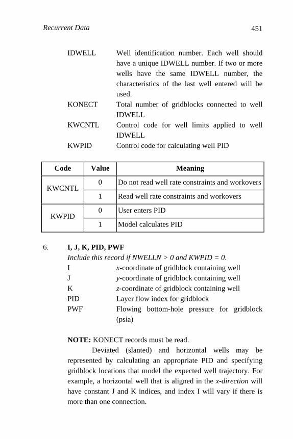
Recurrent Data
451
IDWELL Well identification number. Each well should have a unique IDWELL number. If two or more wells have the same IDWELL number, the characteristics of the last well entered will be used.
KONECT Total number of gridblocks connected to well IDWELL
KWCNTL Control code for well limits applied to well IDWELL
KWPID Control code for calculating well PID
Code Value Meaning
0 Do not read well rate constraints and workovers KWCNTL
1 Read well rate constraints and workovers
0 User enters PID KWPID
1 Model calculates PID
6. I, J, K, PID, PWF
Include this record if NWELLN > 0 and KWPID = 0. I x-coordinate of gridblock containing well J y-coordinate of gridblock containing well K z-coordinate of gridblock containing well PID Layer flow index for gridblock PWF Flowing bottom-hole pressure for gridblock
(psia)
NOTE: KONECT records must be read. Deviated (slanted) and horizontal wells may be
represented by calculating an appropriate PID and specifying gridblock locations that model the expected well trajectory. For example, a horizontal well that is aligned in the x-direction will have constant J and K indices, and index I will vary if there is more than one connection.

Principles of Applied Reservoir Simulation
452
To shut in a connection, set that connection PID to 0. To shut in a well, set all of its connection PID values to zero.
7A. I, J, K, IWDIR, KHMOD, PIDRW, PIDS, PWF
Include this record if NWELLN > 0 and KWPID = 1. I x-coordinate of gridblock containing well J y-coordinate of gridblock containing well K z-coordinate of gridblock containing well IWDIR Well orientation KHMOD Flow capacity model for PID calculation PIDRW Wellbore radius (ft.) PIDS Well skin (fr.) PWF Flowing bottom-hole pressure for gridblock
(psia)
Code Value Meaning
1 Well aligned in x-direction
2 Well aligned in y-direction IWDIR
3 Well aligned in z-direction
0 PID calculated with constant KH KHMOD
1 PID calculated with pressure dependent KH
NOTE: The x-direction φ-K model is
( )[ ]
⎪⎭
⎪⎬⎫
⎪⎩
⎪⎨⎧
+⎟⎟⎠
⎞⎜⎜⎝
⎛
φφ
= φ−φ 02
1
20
10b
b
xx eaaKK
where Kx0 is the initial permeability and φ0 is initial porosity.
Similar models apply to y-direction and z-direction
permeabilities. Coefficients for the directional φ-K models are specified below. Values of net thickness and permeability in well PID are calculated as functions of pressure and saturation when KPHIMOD > 0.
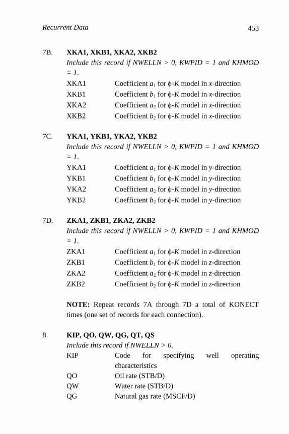
Recurrent Data
453
7B. XKA1, XKB1, XKA2, XKB2 Include this record if NWELLN > 0, KWPID = 1 and KHMOD
= 1.
XKA1 Coefficient a1 for φ-K model in x-direction
XKB1 Coefficient b1 for φ-K model in x-direction
XKA2 Coefficient a2 for φ-K model in x-direction
XKB2 Coefficient b2 for φ-K model in x-direction 7C. YKA1, YKB1, YKA2, YKB2
Include this record if NWELLN > 0, KWPID = 1 and KHMOD
= 1.
YKA1 Coefficient a1 for φ-K model in y-direction
YKB1 Coefficient b1 for φ-K model in y-direction
YKA2 Coefficient a2 for φ-K model in y-direction
YKB2 Coefficient b2 for φ-K model in y-direction 7D. ZKA1, ZKB1, ZKA2, ZKB2
Include this record if NWELLN > 0, KWPID = 1 and KHMOD
= 1.
ZKA1 Coefficient a1 for φ-K model in z-direction
ZKB1 Coefficient b1 for φ-K model in z-direction
ZKA2 Coefficient a2 for φ-K model in z-direction
ZKB2 Coefficient b2 for φ-K model in z-direction
NOTE: Repeat records 7A through 7D a total of KONECT times (one set of records for each connection).
8. KIP, QO, QW, QG, QT, QS
Include this record if NWELLN > 0. KIP Code for specifying well operating
characteristics QO Oil rate (STB/D) QW Water rate (STB/D) QG Natural gas rate (MSCF/D)
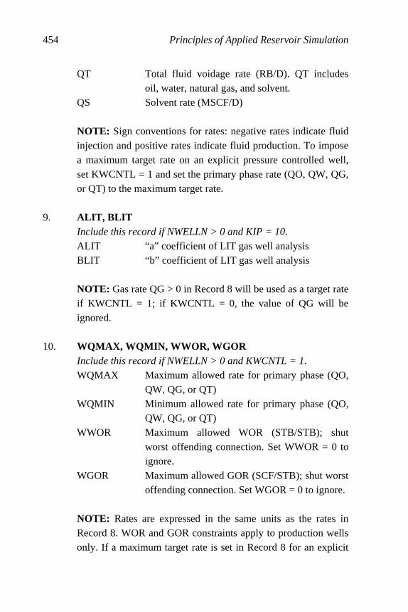
Principles of Applied Reservoir Simulation
454
QT Total fluid voidage rate (RB/D). QT includes oil, water, natural gas, and solvent.
QS Solvent rate (MSCF/D) NOTE: Sign conventions for rates: negative rates indicate fluid injection and positive rates indicate fluid production. To impose a maximum target rate on an explicit pressure controlled well, set KWCNTL = 1 and set the primary phase rate (QO, QW, QG, or QT) to the maximum target rate.
9. ALIT, BLIT
Include this record if NWELLN > 0 and KIP = 10. ALIT “a” coefficient of LIT gas well analysis BLIT “b” coefficient of LIT gas well analysis
NOTE: Gas rate QG > 0 in Record 8 will be used as a target rate if KWCNTL = 1; if KWCNTL = 0, the value of QG will be ignored.
10. WQMAX, WQMIN, WWOR, WGOR
Include this record if NWELLN > 0 and KWCNTL = 1. WQMAX Maximum allowed rate for primary phase (QO,
QW, QG, or QT) WQMIN Minimum allowed rate for primary phase (QO,
QW, QG, or QT) WWOR Maximum allowed WOR (STB/STB); shut
worst offending connection. Set WWOR = 0 to ignore.
WGOR Maximum allowed GOR (SCF/STB); shut worst offending connection. Set WGOR = 0 to ignore.
NOTE: Rates are expressed in the same units as the rates in Record 8. WOR and GOR constraints apply to production wells only. If a maximum target rate is set in Record 8 for an explicit

Recurrent Data
455
pressure controlled well, the value of WQMAX will take precedence.
Records 4 through 10 should be repeated NWELLN times. 11. Heading Up to 80 characters.
Include this record if NWELLO > 0. 12. WELLID
Include this record if NWELLO > 0. WELLID Well name with up to five characters.
13. IDWELL, KONECT, KWCNTL
Include this record if NWELLO > 0. IDWELL Well identification number KONECT Total number of gridblocks connected to well
IDWELL KWCNTL Control code for well limits applied to well
IDWELL 14. I, J, K, PID, PWF
Include this record if NWELLO > 0 and KWPID = 0. I x-coordinate of gridblock containing well J y-coordinate of gridblock containing well K z-coordinate of gridblock containing well PID Layer flow index for gridblock. PWF Flowing bottom-hole pressure for gridblock
(psia).
NOTE: KONECT records must be read. 15A. I, J, K, IWDIR, KHMOD, PIDRW, PIDS, PWF
Include this record if NWELLO > 0 and KWPID = 1. I x-coordinate of gridblock containing well J y-coordinate of gridblock containing well
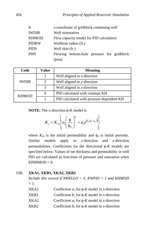
Principles of Applied Reservoir Simulation
456
K z-coordinate of gridblock containing well IWDIR Well orientation KHMOD Flow capacity model for PID calculation PIDRW Wellbore radius (ft.) PIDS Well skin (fr.) PWF Flowing bottom-hole pressure for gridblock
(psia)
Code Value Meaning
1 Well aligned in x-direction
2 Well aligned in y-direction IWDIR
3 Well aligned in z-direction
0 PID calculated with constant KH KHMOD
1 PID calculated with pressure dependent KH
NOTE: The x-direction φ-K model is
( )[ ]
⎪⎭
⎪⎬⎫
⎪⎩
⎪⎨⎧
+⎟⎟⎠
⎞⎜⎜⎝
⎛
φφ
= φ−φ 02
1
20
10b
b
xx eaaKK
where Kx0 is the initial permeability and φ0 is initial porosity.
Similar models apply to y-direction and z-direction
permeabilities. Coefficients for the directional φ-K models are specified below. Values of net thickness and permeability in well PID are calculated as functions of pressure and saturation when KPHIMOD > 0.
15B. XKA1, XKB1, XKA2, XKB2
Include this record if NWELLO > 0, KWPID = 1 and KHMOD
= 1.
XKA1 Coefficient a1 for φ-K model in x-direction
XKB1 Coefficient b1 for φ-K model in x-direction
XKA2 Coefficient a2 for φ-K model in x-direction
XKB2 Coefficient b2 for φ-K model in x-direction
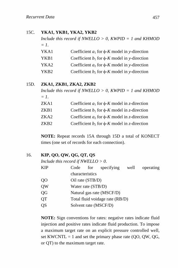
Recurrent Data
457
15C. YKA1, YKB1, YKA2, YKB2 Include this record if NWELLO > 0, KWPID = 1 and KHMOD
= 1.
YKA1 Coefficient a1 for φ-K model in y-direction
YKB1 Coefficient b1 for φ-K model in y-direction
YKA2 Coefficient a2 for φ-K model in y-direction
YKB2 Coefficient b2 for φ-K model in y-direction 15D. ZKA1, ZKB1, ZKA2, ZKB2
Include this record if NWELLO > 0, KWPID = 1 and KHMOD
= 1.
ZKA1 Coefficient a1 for φ-K model in z-direction
ZKB1 Coefficient b1 for φ-K model in z-direction
ZKA2 Coefficient a2 for φ-K model in z-direction
ZKB2 Coefficient b2 for φ-K model in z-direction
NOTE: Repeat records 15A through 15D a total of KONECT times (one set of records for each connection).
16. KIP, QO, QW, QG, QT, QS
Include this record if NWELLO > 0. KIP Code for specifying well operating
characteristics QO Oil rate (STB/D) QW Water rate (STB/D) QG Natural gas rate (MSCF/D) QT Total fluid voidage rate (RB/D) QS Solvent rate (MSCF/D) NOTE: Sign conventions for rates: negative rates indicate fluid injection and positive rates indicate fluid production. To impose a maximum target rate on an explicit pressure controlled well, set KWCNTL = 1 and set the primary phase rate (QO, QW, QG, or QT) to the maximum target rate.

Principles of Applied Reservoir Simulation
458
17. ALIT, BLIT Include this record if NWELLO > 0 and KIP = 10. ALIT “a” coefficient of LIT gas well analysis BLIT “b” coefficient of LIT gas well analysis
NOTE: Gas rate QG > 0 in Record 16 will be used as a target rate if KWCNTL = 1; if KWCNTL = 0, the value of QG will be ignored.
18. WQMAX, WQMIN, WWOR, WGOR
Include this record if NWELLO > 0 and KWCNTL = 1. WQMAX Maximum allowed rate for primary phase (QO,
QW, QG, or QT) WQMIN Minimum allowed rate for primary phase (QO,
QW, QG, or QT) WWOR Maximum allowed WOR (STB/STB); shut
worst offending connection. Set WWOR = 0 to ignore.
WGOR Maximum allowed GOR (SCF/STB); shut worst offending connection. Set WGOR = 0 to ignore.
NOTE: Rates are expressed in the same units as the rates in Record 16. WOR and GOR constraints apply to production wells only. If a maximum target rate is set in Record 16 for an explicit pressure controlled well, the value of WQMAX will take precedence.
Records 12 through 18 should be repeated NWELLO times.

Recurrent Data
459
Table 22-1. Options for Controlling Production Wells
Primary Phase
Well Control KIP Non-Zero
Rates Well
Controls?
Rate 1 QO > 0 Yes
Explicit P -1 QO > 0 Yes Oil
Implicit P -11 No
Rate 1 QG > 0 Yes
Explicit P -1 QG > 0 Yes
Implicit P No Gas
LIT 10 QG > 0 Yes
Rate 1 QW > 0 Yes
Explicit P -1 QW > 0 Yes Water
Implicit P No
Rate 1 QT > 0 Yes
Explicit P -1 QT > 0 Yes Total OWG
Implicit P No

Principles of Applied Reservoir Simulation
460
Table 22-2. Options for Controlling Injection Wells
Primary Phase
Well Control
KIP Non-Zero
Rates Well
Controls?
Rate 2 QW < 0 Yes
Explicit P -2 QW < 0 Yes Water
Implicit P -12 No
Rate 3 QG < 0 Yes
Explicit P -3 QG < 0 Yes Gas
Implicit P -13 No
Rate 100 QS < 0 No
Explicit P -4 No Base Solvent (Solvent 1)
Implicit P -14 No
Rate 200 QS < 0 No
Explicit P -5 No Solvent 2
Implicit P -15 No
Rate 300 QS < 0 No
Explicit P -6 No Solvent 3
Implicit P -16 No
Rate 400 QS < 0 No
Explicit P -7 No Solvent 4
Implicit P -17 No

461
Appendix A: Unit Conversion Factors
TIME 1 hour = 1 hr = 3600 s
1 day = 8.64 × 10⁴ s
1 year = 1 yr = 3.1536 × 10⁷ s
LENGTH 1 foot = 1 ft = 0.3048 m 1 kilometer = 1 km = 1000 m 1 mile = 1 mi = 1.609 km VELOCITY 1 foot per second = 0.3048 m/s 1 kilometer per hour = 1 kph = 1000 m/hr = 0.278 m/s 1 mile per hour = 1 mph = 1.609 km/hr = 1609 m/hr = 0.447 m/s AREA 1 square foot = 1 ft2 = 0.0929 m2
1 square mile = 1 mi2 = 2.589 km2 = 2.589 × 10⁶ m2
1 square mile = 1 mi2 = 640 acres 1 acre = 1 ac = 4047 m2
1 hectare = 1 ha = 1.0 × 10⁴ m2
462 Principles of Applied Reservoir Simulation
1 millidarcy = 1 md = 0.986923 × 10⁻¹⁵ m2
1 Darcy = 1000 md = 0.986923 × 10⁻¹² m2 VOLUME 1 liter = 1 L = 0.001 m3
1 cubic foot = 1 ft3 = 2.83 × 10⁻² m3
1 standard cubic foot = 1 SCF = 1 ft3 at standard conditions 1 acre-foot = 1 ac-ft = 1233.5 m3 1 barrel = 1 bbl = 0.1589 m3
1 gallon (U.S. liquid) = 1 gal = 3.785 × 10⁻³ m3
1 barrel = 42 gallons = 0.1589 m3 MASS 1 gram = 1 g = 0.001 kg 1 pound (avoirdupois) = 1 lb (avdp) = 1 lbm = 0.453592 kg 1 tonne = 1000 kg MASS DENSITY 1 g/cm3 = 1000 kg/m3
FORCE 1 pound-force = 1 lbf = 4.4482 N PRESSURE 1 Pascal = 1 Pa = 1 N/m2 = 1 kg/m┳s2 1 Megapascal = 1 MPa = 106 Pa 1 Gigapascal = 1 GPa = 109 Pa 1 pound-force per square inch = 1 psi = 6894.8 Pa
1 atmosphere = 1 atm = 1.01325 × 10⁵ Pa 1 atmosphere = 1 atm =14.7 psi ENERGY 1 BTU = 1055 J 1 calorie (thermochemical) = 1 cal = 4.184 J
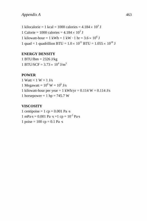
Appendix A 463
1 kilocalorie = 1 kcal = 1000 calories = 4.184 × 10³ J
1 Calorie = 1000 calories = 4.184 × 10³ J
1 kilowatt-hour = 1 kWh = 1 kW · 1 hr = 3.6 × 10⁶ J
1 quad = 1 quadrillion BTU = 1.0 × 10¹⁵ BTU = 1.055 × 10¹⁸ J ENERGY DENSITY 1 BTU/lbm = 2326 J/kg
1 BTU/SCF = 3.73 × 10⁴ J/m3
POWER 1 Watt = 1 W = 1 J/s 1 Megawatt = 106 W = 106 J/s 1 kilowatt-hour per year = 1 kWh/yr = 0.114 W = 0.114 J/s 1 horsepower = 1 hp = 745.7 W VISCOSITY 1 centipoise = 1 cp = 0.001 Pa ·s 1 mPa·s = 0.001 Pa ·s =1 cp = 10-3 Pa·s 1 poise = 100 cp = 0.1 Pa ·s
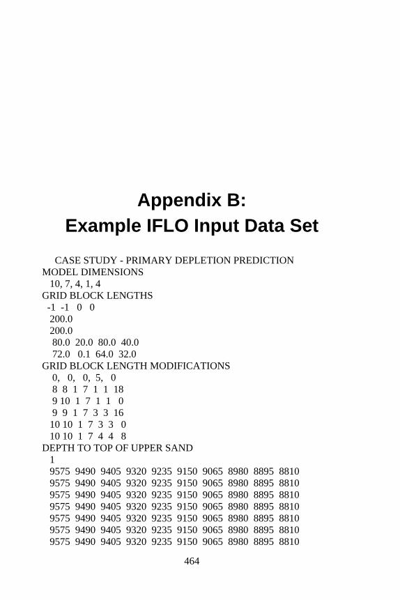
464
Appendix B: Example IFLO Input Data Set
CASE STUDY - PRIMARY DEPLETION PREDICTION MODEL DIMENSIONS 10, 7, 4, 1, 4 GRID BLOCK LENGTHS -1 -1 0 0 200.0 200.0 80.0 20.0 80.0 40.0 72.0 0.1 64.0 32.0 GRID BLOCK LENGTH MODIFICATIONS 0, 0, 0, 5, 0 8 8 1 7 1 1 18 9 10 1 7 1 1 0 9 9 1 7 3 3 16 10 10 1 7 3 3 0 10 10 1 7 4 4 8 DEPTH TO TOP OF UPPER SAND 1 9575 9490 9405 9320 9235 9150 9065 8980 8895 8810 9575 9490 9405 9320 9235 9150 9065 8980 8895 8810 9575 9490 9405 9320 9235 9150 9065 8980 8895 8810 9575 9490 9405 9320 9235 9150 9065 8980 8895 8810 9575 9490 9405 9320 9235 9150 9065 8980 8895 8810 9575 9490 9405 9320 9235 9150 9065 8980 8895 8810 9575 9490 9405 9320 9235 9150 9065 8980 8895 8810
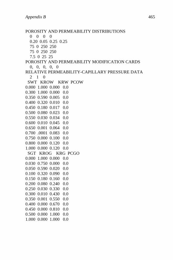
Appendix B 465
POROSITY AND PERMEABILITY DISTRIBUTIONS 0 0 0 0 0.20 0.05 0.25 0.25 75 0 250 250 75 0 250 250 7.5 0 25 25 POROSITY AND PERMEABILITY MODIFICATION CARDS 0, 0, 0, 0, 0 RELATIVE PERMEABILITY-CAPILLARY PRESSURE DATA 2 1 0 SWT KROW KRW PCOW 0.000 1.000 0.000 0.0 0.300 1.000 0.000 0.0 0.350 0.590 0.005 0.0 0.400 0.320 0.010 0.0 0.450 0.180 0.017 0.0 0.500 0.080 0.023 0.0 0.550 0.030 0.034 0.0 0.600 0.010 0.045 0.0 0.650 0.001 0.064 0.0 0.700 .0001 0.083 0.0 0.750 0.000 0.100 0.0 0.800 0.000 0.120 0.0 1.000 0.000 0.120 0.0 SGT KROG KRG PCGO 0.000 1.000 0.000 0.0 0.030 0.750 0.000 0.0 0.050 0.590 0.020 0.0 0.100 0.320 0.090 0.0 0.150 0.180 0.160 0.0 0.200 0.080 0.240 0.0 0.250 0.030 0.330 0.0 0.300 0.010 0.430 0.0 0.350 0.001 0.550 0.0 0.400 0.000 0.670 0.0 0.450 0.000 0.810 0.0 0.500 0.000 1.000 0.0 1.000 0.000 1.000 0.0

466 Principles of Applied Reservoir Simulation
PORE VOLUME AND TRANSMISSIBILITY MODIFICATIONS 11, 0, 0, 2, 0 1 2 1 1 1 4 0.9 3 4 1 1 1 4 0.7 5 6 1 1 1 4 0.5 7 8 1 1 1 4 0.3 9 10 1 1 1 4 0.1 1 1 2 3 1 4 0.8 1 1 4 6 1 4 0.7 1 1 7 7 1 4 0.3 2 4 7 7 1 4 0.6 5 7 7 7 1 4 0.8 8 10 7 7 1 4 0.9 1 10 1 7 2 3 0.0 1 10 1 7 4 4 0.1 PETROPHYSICAL MODEL 0 0 MODULI AND ROCK DENSITY -1 -1 -1 -1 3E6 3E6 3E6 168 CONFINING P AND CLAY CONTENT MODIFICATIONS 3*0 PBO VOSLP BOSLP BWSLP PMAX 2514.7 .000046, -.000023, -3E-6, 6014.7 OIL: P MUO BO RSO 14.7, 1.0400, 1.0620, 1.0 514.7, 0.9100, 1.1110, 89.0 1014.7, 0.8300, 1.1920, 208.0 1514.7, 0.7650, 1.2560, 309.0 2014.7, 0.6950, 1.3200, 392.0 2514.7, 0.6410, 1.3800, 457.0 3014.7, 0.5940, 1.4260, 521.0 4014.7, 0.5100, 1.4720, 586.0 5014.7, 0.4500, 1.4900, 622.0 6014.7, 0.4100, 1.5000, 650.0
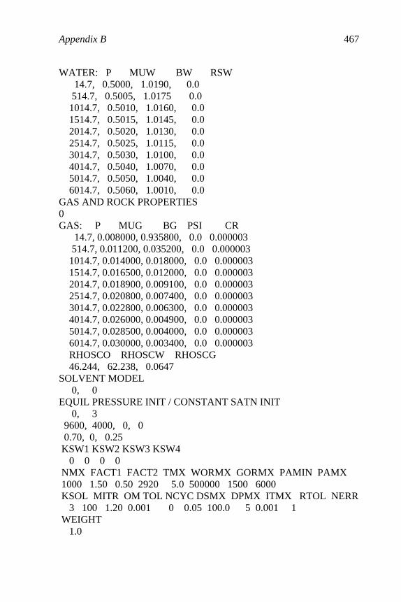
Appendix B 467
WATER: P MUW BW RSW 14.7, 0.5000, 1.0190, 0.0 514.7, 0.5005, 1.0175 0.0 1014.7, 0.5010, 1.0160, 0.0 1514.7, 0.5015, 1.0145, 0.0 2014.7, 0.5020, 1.0130, 0.0 2514.7, 0.5025, 1.0115, 0.0 3014.7, 0.5030, 1.0100, 0.0 4014.7, 0.5040, 1.0070, 0.0 5014.7, 0.5050, 1.0040, 0.0 6014.7, 0.5060, 1.0010, 0.0 GAS AND ROCK PROPERTIES 0 GAS: P MUG BG PSI CR 14.7, 0.008000, 0.935800, 0.0 0.000003 514.7, 0.011200, 0.035200, 0.0 0.000003 1014.7, 0.014000, 0.018000, 0.0 0.000003 1514.7, 0.016500, 0.012000, 0.0 0.000003 2014.7, 0.018900, 0.009100, 0.0 0.000003 2514.7, 0.020800, 0.007400, 0.0 0.000003 3014.7, 0.022800, 0.006300, 0.0 0.000003 4014.7, 0.026000, 0.004900, 0.0 0.000003 5014.7, 0.028500, 0.004000, 0.0 0.000003 6014.7, 0.030000, 0.003400, 0.0 0.000003 RHOSCO RHOSCW RHOSCG 46.244, 62.238, 0.0647 SOLVENT MODEL 0, 0 EQUIL PRESSURE INIT / CONSTANT SATN INIT 0, 3 9600, 4000, 0, 0 0.70, 0, 0.25 KSW1 KSW2 KSW3 KSW4 0 0 0 0 NMX FACT1 FACT2 TMX WORMX GORMX PAMIN PAMX 1000 1.50 0.50 2920 5.0 500000 1500 6000 KSOL MITR OM TOL NCYC DSMX DPMX ITMX RTOL NERR 3 100 1.20 0.001 0 0.05 100.0 5 0.001 1 WEIGHT 1.0
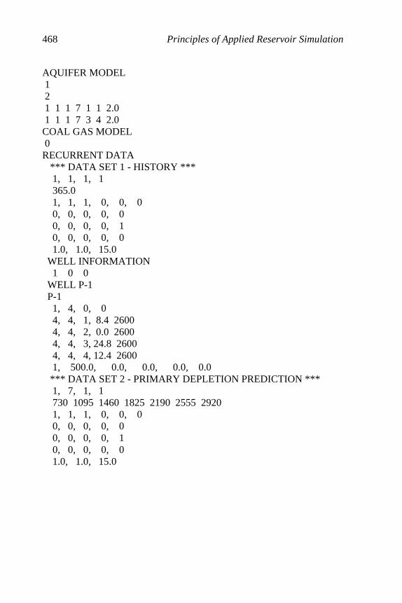
468 Principles of Applied Reservoir Simulation
AQUIFER MODEL 1 2 1 1 1 7 1 1 2.0 1 1 1 7 3 4 2.0 COAL GAS MODEL 0 RECURRENT DATA *** DATA SET 1 - HISTORY *** 1, 1, 1, 1 365.0 1, 1, 1, 0, 0, 0 0, 0, 0, 0, 0 0, 0, 0, 0, 1 0, 0, 0, 0, 0 1.0, 1.0, 15.0 WELL INFORMATION 1 0 0 WELL P-1 P-1 1, 4, 0, 0 4, 4, 1, 8.4 2600 4, 4, 2, 0.0 2600 4, 4, 3, 24.8 2600 4, 4, 4, 12.4 2600 1, 500.0, 0.0, 0.0, 0.0, 0.0 *** DATA SET 2 - PRIMARY DEPLETION PREDICTION *** 1, 7, 1, 1 730 1095 1460 1825 2190 2555 2920 1, 1, 1, 0, 0, 0 0, 0, 0, 0, 0 0, 0, 0, 0, 1 0, 0, 0, 0, 0 1.0, 1.0, 15.0

Appendix B 469
WELL INFORMATION 0 1 0 WELL P-1 P-1 1, 4, 0, 0 4, 4, 1, 8.4 2600 4, 4, 2, 0.0 2600 4, 4, 3, 24.8 2600 4, 4, 4, 12.4 2600 1, 500.0, 0.0, 0.0, 0.0, 0.0

470
References Abramowitz, M.A. and I.A. Stegun (1972): Handbook of Mathematical
Functions, ninth printing, New York: Dover. Aguilera, R. (1980): Naturally Fractured Reservoirs, Tulsa,
Oklahoma: PennWell Publishing. Aguilera, R. (July 1999): “Recovery Factors and Reserves in Naturally
Fractured Reservoirs,” Journal of Canadian Petroleum
Technology, pages 15-18. Ahmed, T. (2000): Reservoir Engineering Handbook, Houston, Texas:
Gulf Publishing. Akin, S. (2001): “Estimation of Fracture Relative Permeabilities from
Unsteady State Corefloods,” Journal of Petroleum Science and
Engineering, Volume 30, pages 1-14. Al-Hussainy, R. and N. Humphreys (1996): “Reservoir Management:
Principles and Practices,” Journal of Petroleum Technology, pages 1129-1135.
Al-Marhoun, M.A. (June 2003): “Adjustment of Differential Liberation Data to Separator Conditions,” SPE Reservoir Evaluation &
Engineering, pages 142-146. Allan, J. and S.Q. Sun (2003): “Controls on Recovery Factor in
Fractured Reservoirs: Lessons Learned from 100 Fractured Fields,” Paper SPE 84590, presented at the 2003 SPE Annual Technical Conference and Exhibition, Richardson, Texas: Society of Petroleum Engineers.
References 471
Ammer, J.R., A.C. Brummert and W.N. Sams (1991): “Miscible Applied Simulation Techniques for Energy Recovery – Version 2.0,” U.S. Department of Energy Report DOE/BC-91/2/SP, Morgantown Energy Technology Center, West Virginia.
Amyx, J.W., D.H. Bass, and R.L. Whiting (1960): Petroleum Reservoir Engineering, New York: McGraw-Hill.
Ancell, K.L., S. Lambert, and F.S. Johnson (1980): “Analysis of the Coalbed Degasification Process at a Seventeen Well Pattern in the Warrior Basin of Alabama,” Paper SPE/DOE 8971, presented at the 1980 SPE/DOE Symposium on Unconventional Gas Recovery, Pittsburgh, Pennsylvania (18-21 May); Richardson, Texas: Society of Petroleum Engineers.
Anderson, R.N. (1995): “Method Described for using 4D Seismic to Track Reservoir Fluid Movement,” Oil & Gas Journal, pages 70-74, April 3.
Arps, J.J. (1945): “Analysis of Decline Curves,” Transaction of AIME, Volume 160, pages 228-247.
Asquith, G. And D. Krygowski (2004): Basic Well Log Analysis for Geologists, Tulsa, Oklahoma: American Association of Petroleum Geologists.
Ates, H., A. Bahar, S. El-Abd, M. Charfeddine, M. Kelkar, ad A. Datta-Gupta (February 2005): “Ranking and Upscaling of Geostatistical Reservoir Models by Use of Streamline Simulation: A Field Case Study,” SPE Reservoir Evaluation & Engineering, pages 22-32.
Ausburn, B.E., A.K. Nath and T.R. Wittick (November 1978): “Modern Seismic Methods – An Aid for the Petroleum Engineer,” Journal
of Petroleum Technology, pages 1519-1530. Aziz, K. (1993): “Reservoir Simulation Grids: Opportunities and
Problems,” Journal of Petroleum Technology, pages 658-663. Aziz, K., Z.E. Heinemann, C. Wolfsteiner, and M.J. Mlacnik (February
2002): “The Changing World of Reservoir Simulation,” Journal of
Petroleum Technology, pages 26-28. Aziz, K. and A. Settari (1979): Petroleum Reservoir Simulation, New
York: Elsevier.

472 Principles of Applied Reservoir Simulation
Babu, D.K. and A. S. Odeh (1989): “Productivity of a Horizontal Well,” Society of Petroleum Engineers Journal, pages 417-421.
Barree, R.D. and M.W. Conway (March 2005): “Beyond Beta Factors: A Model for Darcy, Forchheimer, and Trans-Forchheimer Flow in Porous Media,” Journal of Petroleum Technology, pages 43-45.
Bashore, W.M. (2000): “Data Integration Realizes the Promise of Multidisciplinary Efforts,” Paper OTC 11956, presented at the Offshore Technology Conference, Houston, 1 – 4 May.
Bassiouni, Z. (1994): Theory, Measurement, and Interpretation of Well Logs, Richardson, Texas: Society of Petroleum Engineers.
Bear, J. (1972): Dynamics of Fluids in Porous Media, New York: Elsevier.
Beasley, C.J. (1996): “Seismic Advances Aid Reservoir Description,” Journal of Petroleum Technology, pages 29-30.
Beggs, H.D. (1991): Production Optimization Using Nodal Analysis, Tulsa, Oklahoma: OGCI Publications.
Beggs, H.D., and J.P. Brill (May 1973): “A Study of Two-Phase Flow in Inclined Pipes,” Journal of Petroleum Technology, page 607.
Benedict, M., G.B. Webb, and L.C. Rubin (1940): Journal of Chemical
Physics, Volume 8, page 334. Blackwelder, B., L. Canales, and J. Dubose (1996): “New Technologies
in Reservoir Characterization,” Journal of Petroleum Technology, pages 26-27.
Blunt, M.J. (1999): “An Empirical Model for Three-Phase Relative Permeability,” Paper SPE 56474, presented at the 1999 Annual Technical Conference and Exhibition of the Society of Petroleum Engineers, Richardson, Texas: Society of Petroleum Engineers.
Bradley, M.E. and A.R.O. Wood (November 1994): “Forecasting Oil Field Economic Performances,” Journal of Petroleum Technology, pages 965-971 and references therein.
Brill, J.P. (January 1987): “Multiphase Flow in Wells,” Journal of
Petroleum Technology, pages 15-21. Brill, J.P., and S.J. Arirachakaran (May 1992): “State of the Art in
Multiphase Flow,” Journal of Petroleum Technology, pages 538-541.

References 473
Brill, J.P., and H. Mukherjee (1999): Multiphase Flow in Wells, SPE Monograph Volume 17, Richardson, Texas: Society of Petroleum Engineers.
Brown, K.E. and J.F. Lea (October 1985): “Nodal Systems Analysis of Oil and Gas Wells,” Journal of Petroleum Technology, pages 1751-1763.
Brown, L.P. and R.V. Hawkes (May 2005): “Rules of Thumb in Well Testing: What Works and Doesn’t Work – and Why,” Journal of
Canadian Petroleum Technology, pages 51-55. Brownlee, M.H. and L.A. Sugg (1987): “East Vacuum Grayburg-San
Andres Unit CO2 Injection Project: Development and Results to Date,” Paper SPE 16721, presented at the 62nd Annual Technical Conference and Exhibition of the Society of Petroleum Engineers, Richardson, Texas: Society of Petroleum Engineers.
Brock, J. (1986): Applied Open-Hole Log Analysis, Houston: Gulf Publishing.
Brundtland, G. (1987): Our Common Future, Oxford University Press, Oxford, United Kingdom.
de Buyl, M., T. Guidish, and F. Bell (1988): “Reservoir Description from Seismic Lithologic Parameter Estimation,” Journal of Petroleum
Technology, pages 475-482. Carlson, M.R. (2003): Practical Reservoir Simulation, Tulsa,
Oklahoma: PennWell. Carr, N.L., R. Kobayashi, and D.B. Burrows (1954): “Viscosity of
Hydrocarbon Gases under Pressure,” Transactions of AIME, Volume 201, pages 264-272.
Carter, R.D. and G.W. Tracy (1960) “An Improved Method for Calculating Water Influx,” Transactions of AIME, Volume 219, pages 415-417.
Chambers, R.L., J.M. Yarus, and K.B. Hird (2000): “Petroleum geostatistics for nongeostatisticians,” The Leading Edge, Part 1, pages 474- 479, May; and Part 2, pages 592-599, June.

474 Principles of Applied Reservoir Simulation
Chase, C. A., Jr. and M. R. Todd (1984): “Numerical Simulation of CO2 Flood Performance,” Society of Petroleum Engineers Journal, pages 597-604.
Chaudhry, A.U. (2003a): Gas Well Testing Handbook, Boston: Elsevier.
Chaudhry, A.U. (2003b): Oil Well Testing Handbook, Boston: Elsevier.
Chawathé, A. and I. Taggart (August 2004): “Insights into Upscaling using 3D Streamlines,” SPE Reservoir Evaluation & Engineering, pages 285-296.
Chin, W.C. (1993): Modern Reservoir Flow and Well Transient Analysis, Houston: Gulf Publishing.
Christie, M.A. (November 1996): “Upscaling for Reservoir Simulation,” Journal of Petroleum Technology, pages 1004-1010.
Christie, M.A. and M.J. Blunt (2001): “Tenth SPE Comparative Solution Project: A Comparison of Upscaling Techniques,” Paper SPE 66599, presented at the 2001 SPE Reservoir Simulation Symposium, Richardson, Texas: Society of Petroleum Engineers.
Chorn, L.G. and M. Croft (August 2000): “Resolving Reservoir Uncertainty to Create Value,” Journal of Petroleum Technology, pages 52-59.
Chu, W.C. (September, 2000): “Pressure-transient Testing Ideal for Reservoir Management,” Hart’s E&P, pages 47-50.
Clark, I. and W. Harper (2000): Practical Geostatistics 2000 Book and CD, Columbus, Ohio: Ecosse North America, LLC.
Clark, N.J. (1969): Elements of Petroleum Reservoirs, Richardson, Texas: Society of Petroleum Engineers.
Coats, K.H. (1969): “Use and Misuse of Reservoir Simulation Models,” Journal of Petroleum Technology, pages 183-190.
Cope, G. (2001): “Improving Efficiency through Reservoir Modeling and Production Simulation,” Journal of Canadian Petroleum
Technology, pages 7-11. Collins, R.E. (1961): Flow of Fluids through Porous Materials, Tulsa,
Oklahoma: Petroleum Publishing-Reinhold.

References 475
Craft, B.C., M.F. Hawkins, and R.E. Terry (1991): Applied Petroleum Reservoir Engineering, Second Edition, Englewood Cliffs, New Jersey: Prentice-Hall.
Craig, F.F. (1971): The Reservoir Engineering Aspects of Waterflooding, SPE Monograph Series, Richardson, Texas: Society of Petroleum Engineers.
Craig, F.F., P.J. Wilcox, J.R. Ballard and W.R. Nation (July 1977): “Optimized Recovery through Continuing Interdisciplinary Cooperation,” Journal of Petroleum Technology, pages 755-760.
Crichlow, H.B. (1977): Modern Reservoir Engineering – A Simulation Approach, Englewood Cliffs, New Jersey: Prentice Hall.
Daccord, G., J. Nittmann and H.E. Stanley (1986): “Radial Viscous
Fingers and Diffusion-Limited Aggregation: Fractal Dimension and Growth Sites,” Physical Review Letters, Volume 56, 336-339.
Dahlberg, E.C. (1975): “Relative Effectiveness of Geologists and Computers in Mapping Potential Hydrocarbon Exploration Targets,” Mathematical Geology, Volume 7, pages 373-394.
Dake, L.P. (1978): Fundamentals of Reservoir Engineering, Amsterdam: Elsevier.
Dake, L.P. (2001): The Practice of Reservoir Engineering, Revised Edition, Amsterdam: Elsevier.
Dean, R.H., X. Gai, C.M. Stone and E. Minkoff (2003), “A Comparison of Techniques for Coupling Porous Flow and Geomechanics,” Paper SPE 79709, presented at the SPE Reservoir Simulation Symposium, Richardson, Texas: Society of Petroleum Engineers.
Deghmoum, A.H., D. Tiab, and A. Mazouzi (December 2001): “Relative Permeability in Dual Porosity Porous Media,” Journal of
Canadian Petroleum Technology, pages 32-42. Deutsch, C.V. and A.G. Journel (1998): GSLIB: Geostatistical
Software Library and User’s Guide, New York, New York: Oxford University Press.

476 Principles of Applied Reservoir Simulation
Dietrich, J.K. and P.L. Bondor (1976): “Three-Phase Oil Relative Permeability Models,” Paper SPE 6044, presented at the 51st Fall Technical Conference and Exhibition of Society of Petroleum Engineers, Richardson, Texas: Society of Petroleum Engineers.
Dietrich, F.L., F.G. Brown, Z.H. Zhou, M.A. Maure (1996): “Microbial EOR Technology Advancement: Case Studies of Successful Projects,” paper SPE 36746 presented at the 1996 SPE Annual Technical Conference and Exhibition of the Society of Petroleum Engineers, Richardson, Texas: Society of Petroleum Engineers.
Dogru, A.H. (May, 2000): “Megacell Reservoir Simulation,” Journal of
Petroleum Technology, pages 54-60. Dogru, A.H., H.A. Sunaidi, L.S. Fung, W.A. Habiballah, N. Al-Zamel,
and K.G. Li (February 2002): “A Parallel Reservoir Simulator for Large-Scale Reservoir Simulation,” SPE Reservoir Evaluation &
Engineering, pages 11-23. Dorn, G.A. (September, 1998): “Modern 3-D Seismic Interpretation,”
The Leading Edge, pages 1262-1283. Dranchuk, P.M., R.A. Purvis, and D.B. Robinson (1974): “Computer
Calculation of Natural Gas Compressibility Factors Using the Standing and Katz Correlations,” Institute of Petroleum
Technology, IP-74-008. Dubrule, O. (2003): Geostatistics for Seismic Data Integration in
Earth Models, 2003 Distinguished Instructor Short Course, Tulsa: Society of Exploration Geophysicists.
van Dyke, K. (1997): Fundamentals of Petroleum, 4th Edition, The University of Texas at Austin: Petroleum Extension Service.
Earlougher, R.C., Jr. (1977): Advances in Well Test Analysis, SPE
Monograph Series, Richardson, Texas: Society of Petroleum Engineers.
Ebanks, W.J., Jr. (1987): “Flow Unit Concept – Integrated Approach to Reservoir Description for Engineering Projects,” paper presented at the AAPG Annual Meeting, Los Angeles.
References 477
Englund, E. and A. Sparks (1991): “Geo-EAS 1.2.1 User’s Guide,” EPA
Report #600/8-91/008 Environmental Protection Agency-EMSL, Las Vegas, NV.
Ertekin, T., J.H. Abou-Kassem and G.R. King (2001): Basic Applied Reservoir Simulation, Richardson, Texas: Society of Petroleum Engineers.
Evans, S. (May 17, 2004): “Reservoir Modeling and Simulation in Today’s High-Performance Computing Environments,” Oil & Gas
Journal, pages 33-37. Evans, W.S. (1996): “Technologies for Multidisciplinary Reservoir
Characterization,” Journal of Petroleum Technology, pages 24-25. van Everdingen, A.F. and W. Hurst (1949): “The Application of the
Laplace Transformation to Flow Problems in Reservoirs,”
Transactions of AIME, Volume 186, pages 305-324. Fanchi, J.R., K.J. Harpole, and H.B. Carroll (13 September 1982):
“Black-Oil Reservoir Simulator is now Available,” Oil & Gas
Journal, pages 66-68. Fanchi, J.R. (1983): “Multidimensional Numerical Dispersion,” Society
of Petroleum Engineering Journal, pages 143-151. Fanchi, J.R. (June 1985): “Analytical Representation of the van
Everdingen-Hurst Aquifer Influence Functions for Reservoir Simulation,” Society of Petroleum Engineering Journal, pages 405-406.
Fanchi, J.R. (1986): “BOAST-DRC: Black Oil and Condensate Reservoir Simulation on an IBM-PC,” Paper SPE 15297, presented at the Symposium on Petroleum Industry Applications of Microcomputers of the Society of Petroleum Engineers, Richardson, Texas: Society of Petroleum Engineers.
Fanchi, J.R. (1990): “Calculation of Parachors for Compositional Simulation: An Update,” Society of Petroleum Engineers
Reservoir Engineering, pages 433-436. Fanchi, J.R. (1999): “Flow Models Time 4-D Seismic Surveys,” Oil &
Gas Journal, pages 46-51.
478 Principles of Applied Reservoir Simulation
Fanchi, J.R. (2000): Integrated Flow Modeling, Amsterdam: Elsevier. Fanchi, J.R. (2002a): Shared Earth Modeling, Boston: Butterworth-
Heinemann-Elsevier. Fanchi, J.R. (2002b): “Estimating Subsidence during Coalbed Methane
Production,” Paper SPE 75511, presented at the SPE Gas Technology Symposium, Richardson, Texas: Society of Petroleum Engineers.
Fanchi, J.R. (2003a): "The Han-Eberhart-Phillips model and integrated flow modeling," Geophysics, Volume 68, pages 574-576.
Fanchi, J.R. (2003b): “Feasibility of Monitoring CO2 Sequestration in a Mature Oil Field using Time-Lapse Seismic Analysis,” Paper SPE 66569, presented at SPE/EPA/DOE Exploration and Production Environmental Conference, Richardson, Texas: Society of Petroleum Engineers.
Fanchi, J.R. (2003c): “Estimating Geomechanical Properties Using an Integrated Flow Model,” SPE Reservoir Evaluation and
Engineering, pages 108-116. Fanchi, J.R. (2004): Energy: Technology and Directions for the
Future, Boston: Elsevier-Academic Press. Fanchi, J.R. (2006): Math Refresher for Scientists and Engineers,
Third Edition , New York: J. Wiley and Sons. Fanchi, J.R. and R.L. Christiansen (1989): “Applicability of Fractals to
the Description of Viscous Fingering,” Paper SPE 19782, presented at the 64th Annual Technical Conference and Exhibition of Society of Petroleum Engineers, Richardson, Texas: Society of Petroleum Engineers.
Fanchi, J.R., K.J. Harpole, and S.W. Bujnowski (1982): “BOAST: A Three- Dimensional, Three-Phase Black Oil Applied Simulation Tool,” 2 Volumes, U.S. Department of Energy, Bartlesville Energy Technology Center, Oklahoma.
Fanchi, J.R., J.E. Kennedy, and D.L. Dauben (1987): “BOAST II: A Three-Dimensional, Three-Phase Black Oil Applied Simulation Tool,” U.S. Department of Energy, Bartlesville Energy Technology Center, Oklahoma.
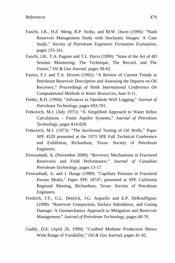
References 479
Fanchi, J.R., H.Z. Meng, R.P. Stoltz, and M.W. Owen (1996): “Nash Reservoir Management Study with Stochastic Images: A Case Study,” Society of Petroleum Engineers Formation Evaluation, pages 155-161.
Fanchi, J.R., T.A. Pagano and T.L. Davis (1999): “State of the Art of 4D Seismic Monitoring: The Technique, The Record, and The Future,” Oil & Gas Journal, pages 38-43.
Fayers, F.J. and T.A. Hewett (1992): “A Review of Current Trends in Petroleum Reservoir Description and Assessing the Impacts on Oil Recovery,” Proceedings of Ninth International Conference On
Computational Methods in Water Resources, June 9-11. Felder, R.D. (1994): “Advances in Openhole Well Logging,” Journal of
Petroleum Technology, pages 693-701. Fetkovich, M.J. (July 1971): “A Simplified Approach to Water Influx
Calculations – Finite Aquifer Systems,” Journal of Petroleum
Technology, pages 814-828. Fetkovich, M.J. (1973): “The Isochronal Testing of Oil Wells,” Paper
SPE 4529 presented at the 1973 SPE Fall Technical Conference and Exhibition, Richardson, Texas: Society of Petroleum Engineers.
Firoozabadi, A. (November 2000): “Recovery Mechanisms in Fractured Reservoirs and Field Performance,” Journal of Canadian
Petroleum Technology, pages 13-17. Firoozabadi, A. and J. Hauge (1989): "Capillary Pressure in Fractured
Porous Media," Paper SPE 18747, presented at SPE California Regional Meeting, Richardson, Texas: Society of Petroleum Engineers.
Fredrich, J.T., G.L. Deitrick, J.G. Arguello and E.P. DeRouffignac (1998): “Reservoir Compaction, Surface Subsidence, and Casing Damage: A Geomechanics Approach to Mitigation and Reservoir Management,” Journal of Petroleum Technology, pages 68-70.
Gaddy, D.E. (April 26, 1999): “Coalbed Methane Production Shows
Wide Range of Variability,” Oil & Gas Journal, pages 41-42.

480 Principles of Applied Reservoir Simulation
Ganzer, L.J. (2002): “Simulating Fractured Reservoirs using Adaptive Dual Continuum,” Paper SPE 75233, presented at the SPE/DOE Improved Oil Recovery Symposium, Richardson, Texas: Society of Petroleum Engineers.
Gardner, H.F., L.W. Gardner, and A.H. Gregory (1974): “Formation Velocity and Density – the Diagnostic Basis for Stratigraphic Traps,” Geophysics Volume 39, pages 770-780.
Gassmann, F. (1951): “Elastic Waves through a Packing of Spheres,” Geophysics, Volume 16, pages 673-685.
Gilbert, W.E. (1954): “Flowing and Gas-Lift Well Performance,” Drilling and Production Practices, page 126 ff.
Gilman, J.R., H-Z. Meng, M.J. Uland, P.J. Dzurman, and S. Cosic (2002): “Statistical Ranking of Stochastic Geomodels using Streamline Simulation: A Field Application,” Paper SP 77374, presented at the 2002 Annual Technical Conference and Exhibition of Society of Petroleum Engineers, Richardson, Texas: Society of Petroleum Engineers.
Golan, M. (2000): Keynote address to the Productivity Enhancement Session, Improved Recovery Symposium (IRS) 2000, sponsored by ONGC (Oil and Natural Gas Corporation), Ahmedabad, India, July.
Golf-Racht, T.D. van (1982): Fundamentals of Fractured Reservoir Engineering, New York: Elsevier.
Govier, G.W., Editor (1978): Theory and Practice of the Testing of Gas Wells, Calgary: Energy Resources Conservation Board.
Grace, J.D., R.H. Caldwell, and D.I. Heather (Sept. 1993): “Comparative Reserves Definitions: USA, Europe, and the Former Soviet Union,” Journal of Petroleum Technology, pages 866-872.
Green, D.W. and G.P. Wilhite (1998): Enhanced Oil Recovery, Richardson, Texas: Society of Petroleum Engineers.
Griffith, P. (March 1984), “Multiphase Flow in Pipes,” Journal of
Petroleum Technology, pages 361-367. Grigg, R.B. and D.S. Schechter (1998): “Improved Efficiency of
Miscible CO2 Floods and Enhanced Prospects for CO2 Flooding Heterogeneous Reservoirs,” Report PRRC 98-29, and Annual

References 481
Report to the U.S. Department of Energy for the Period June 1, 1997 through May 31, 1998; National Petroleum Technology Office, Tulsa.
Guan, L., Y. Du, S.G. Johnson, and M.K. Choudhary (May 2005): “Advances of Interwell Tracer Analysis in the Petroleum Industry,” Journal of Canadian Petroleum Technology, pages 12-15.
Guéguen, Y. and V. Palciauskas (1994): Introduction to the Physics of Rocks, Princeton, New Jersey: Princeton University Press.
Guerrero, E.T. (1966): “Material Balance Principles,” Reservoir Engineering Refresher Course, Tulsa: Mid-Continent Section of AIME.
Gunter, G.W., J.M. Finneran, D.J. Hartmann, and J.D. Miller (1997): “Early Determination of Reservoir Flow Units Using an Integrated Petrophysical Method,” Paper SPE 38679, presented at the 1997 SPE Annual Technical Conference and Exhibition of the Society of Petroleum Engineers, Richardson, Texas: Society of Petroleum Engineers.
Haldorsen, H.H. and E. Damsleth (1993): “Challenges in Reservoir
Characterization,” American Association of Petroleum Geologists
Bulletin, Volume 77, No. 4, pages 541-551. Haldorsen, H.H. and E. Damsleth (April 1990): “Stochastic Modeling,”
Journal of Petroleum Technology, pages 404-412. Haldorsen, H.H. and L.W. Lake (1989): “A New Approach to Shale
Management in Field-Scale Models,” Reservoir Characterization 2, SPE Reprint Series #27, Richardson, Texas: Society of Petroleum Engineers.
Harpole, K.J. (1985): Reservoir Environments and Their Characterization, Boston: International Human Resources Development Corporation.
Harris, D.G. (May 1975): “The Role of Geology in Reservoir Simulation Studies,” Journal of Petroleum Technology, pages 625-632.
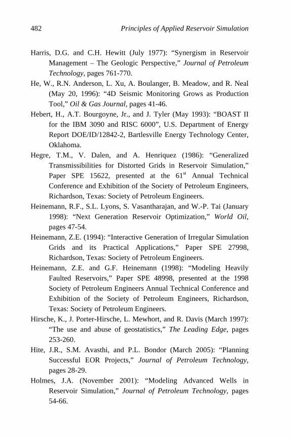
482 Principles of Applied Reservoir Simulation
Harris, D.G. and C.H. Hewitt (July 1977): “Synergism in Reservoir Management – The Geologic Perspective,” Journal of Petroleum
Technology, pages 761-770. He, W., R.N. Anderson, L. Xu, A. Boulanger, B. Meadow, and R. Neal
(May 20, 1996): “4D Seismic Monitoring Grows as Production Tool,” Oil & Gas Journal, pages 41-46.
Hebert, H., A.T. Bourgoyne, Jr., and J. Tyler (May 1993): “BOAST II for the IBM 3090 and RISC 6000”, U.S. Department of Energy Report DOE/ID/12842-2, Bartlesville Energy Technology Center, Oklahoma.
Hegre, T.M., V. Dalen, and A. Henriquez (1986): “Generalized Transmissibilities for Distorted Grids in Reservoir Simulation,” Paper SPE 15622, presented at the 61st Annual Technical Conference and Exhibition of the Society of Petroleum Engineers, Richardson, Texas: Society of Petroleum Engineers.
Heinemann, R.F., S.L. Lyons, S. Vasantharajan, and W.-P. Tai (January 1998): “Next Generation Reservoir Optimization,” World Oil, pages 47-54.
Heinemann, Z.E. (1994): “Interactive Generation of Irregular Simulation Grids and its Practical Applications,” Paper SPE 27998, Richardson, Texas: Society of Petroleum Engineers.
Heinemann, Z.E. and G.F. Heinemann (1998): “Modeling Heavily Faulted Reservoirs,” Paper SPE 48998, presented at the 1998 Society of Petroleum Engineers Annual Technical Conference and Exhibition of the Society of Petroleum Engineers, Richardson, Texas: Society of Petroleum Engineers.
Hirsche, K., J. Porter-Hirsche, L. Mewhort, and R. Davis (March 1997): “The use and abuse of geostatistics,” The Leading Edge, pages 253-260.
Hite, J.R., S.M. Avasthi, and P.L. Bondor (March 2005): “Planning Successful EOR Projects,” Journal of Petroleum Technology, pages 28-29.
Holmes, J.A. (November 2001): “Modeling Advanced Wells in Reservoir Simulation,” Journal of Petroleum Technology, pages 54-66.

References 483
Honarpour, M., L.F. Koederitz, and A.H. Harvey (1982): “Empirical Equations for Estimating Two-Phase Relative Permeability in Consolidated Rock,” Journal of Petroleum Technology, pages 2905-2908.
Horne, R.N. (1995): Modern Well Test Analysis, Palo Alto, California: Petroway.
Hui, M-H., D. Zhou, X-H. Wen, and L.J. Durlofsky (June 2005): “Development and Application of a New Technique for Upscaling Miscible Processes,” SPE Reservoir Evaluation & Engineering, pages 189-195.
Isaaks, E.H. and R.M. Srivastava (1989): Applied Geostatistics, New
York: Oxford University Press. Jack, I. (1998): Time-Lapse Seismic in Reservoir Management, 1998
Distinguished Instructor Short Course, Tulsa: Society of Exploration Geophysicists.
Jefferys, W.H. and J.O. Berger (1992): “Ockham’s Razor and Bayesian Analysis,” American Scientist, Volume 80, pages 64-72.
Jennings, J.W., Jr., and F.J. Lucia (August 2003): “Predicting Permeability from Well Logs in Carbonates with a Link to Geology for Interwell Permeability Mapping,” SPE Reservoir
Evaluation & Engineering, pages 215-225. Johnston, D.H. (1997): “A Tutorial on Time-Lapse Seismic Reservoir
Monitoring,” Journal of Petroleum Technology, pages 473-475. Jones, A.H., G.J. Bell, and R.A. Schraufnagel (1988): “A Review of the
Physical and Mechanical Properties of Coal with Implications for Coal-Bed Methane Well Completion and Production,” Geology and Coal-Bed Methane Resources of the Northern San Juan Basin, New Mexico and Colorado, edited by J.E. Fasset, Rocky Mountain Assoc. of Geologists, 169-81; reprinted in SPE Reprint Series #35 Coalbed Methane, Society of Petroleum Engineers, Richardson, Texas (1992).
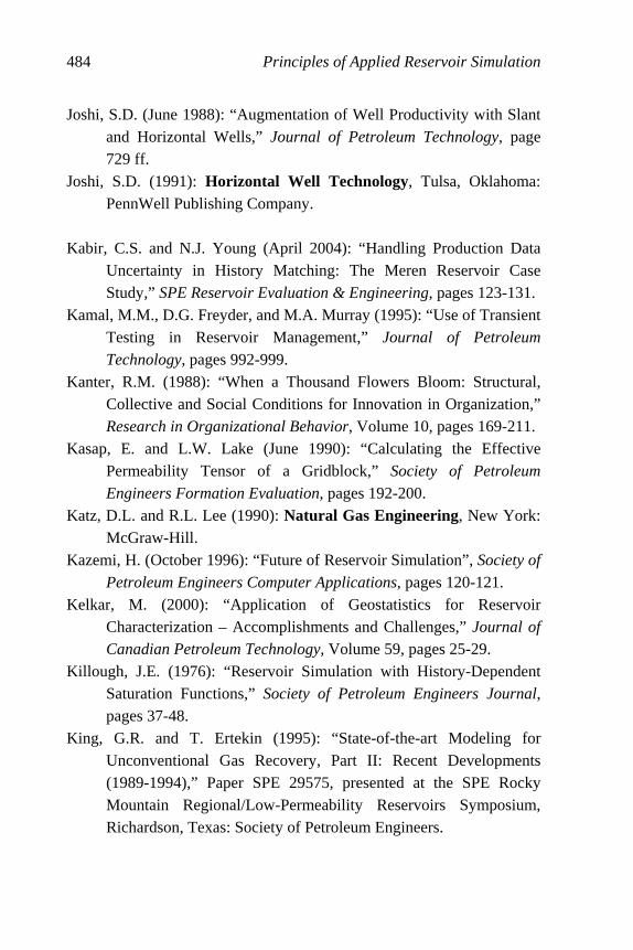
484 Principles of Applied Reservoir Simulation
Joshi, S.D. (June 1988): “Augmentation of Well Productivity with Slant and Horizontal Wells,” Journal of Petroleum Technology, page 729 ff.
Joshi, S.D. (1991): Horizontal Well Technology, Tulsa, Oklahoma: PennWell Publishing Company.
Kabir, C.S. and N.J. Young (April 2004): “Handling Production Data
Uncertainty in History Matching: The Meren Reservoir Case Study,” SPE Reservoir Evaluation & Engineering, pages 123-131.
Kamal, M.M., D.G. Freyder, and M.A. Murray (1995): “Use of Transient Testing in Reservoir Management,” Journal of Petroleum
Technology, pages 992-999. Kanter, R.M. (1988): “When a Thousand Flowers Bloom: Structural,
Collective and Social Conditions for Innovation in Organization,”
Research in Organizational Behavior, Volume 10, pages 169-211. Kasap, E. and L.W. Lake (June 1990): “Calculating the Effective
Permeability Tensor of a Gridblock,” Society of Petroleum
Engineers Formation Evaluation, pages 192-200. Katz, D.L. and R.L. Lee (1990): Natural Gas Engineering, New York:
McGraw-Hill. Kazemi, H. (October 1996): “Future of Reservoir Simulation”, Society of
Petroleum Engineers Computer Applications, pages 120-121. Kelkar, M. (2000): “Application of Geostatistics for Reservoir
Characterization – Accomplishments and Challenges,” Journal of
Canadian Petroleum Technology, Volume 59, pages 25-29. Killough, J.E. (1976): “Reservoir Simulation with History-Dependent
Saturation Functions,” Society of Petroleum Engineers Journal, pages 37-48.
King, G.R. and T. Ertekin (1995): “State-of-the-art Modeling for Unconventional Gas Recovery, Part II: Recent Developments (1989-1994),” Paper SPE 29575, presented at the SPE Rocky Mountain Regional/Low-Permeability Reservoirs Symposium, Richardson, Texas: Society of Petroleum Engineers.

References 485
King, M.J. and M. Mansfield (August 1999): “Flow Simulation of Geologic Models,” SPE Reservoir Evaluation & Engineering, pages 351-367.
Koederitz, L.F., A.H. Harvey, and M. Honarpour (1989): Introduction to Petroleum Reservoir Analysis, Houston: Gulf Publishing.
Kreyszig, E. (1999): Advanced Engineering Mathematics, Eighth Edition , New York: J. Wiley and Sons.
Kuuskraa, V.A. and C.F. Brandenburg (October 9, 1989): “Coalbed Methane Sparks a New Energy Industry,” Oil & Gas Journal, pages 49.
Kuuskraa, V.A. and G.C. Bank (December 8, 2003): “Gas from Tight Sands, Shales a Growing Share of U.S. Supply,” Oil & Gas
Journal, pages 34-43. Lake, L.W. (April 1988): “The Origins of Anisotropy,” Journal of
Petroleum Technology, pages 395-396. Lake, L.W. (1989): Enhanced Oil Recovery, Englewood Cliffs, New
Jersey: Prentice Hall. Lantz, R.B. (1971): “Quantitative Evaluation of Numerical Diffusion,”
Society of Petroleum Engineering Journal, pages 315-320. Lasseter, T.J. and S.A. Jackson (November 2004): “Improving Integrated
Interpretation Accuracy and Efficiency using a Single Consistent Reservoir Model from Seismic to Simulation,” The Leading Edge, pages 1118-1121.
Lea, J., H.V. Nickens, and M. Wells, (2003): Gas Well Deliquification, Burlington, Massachusetts: Elsevier-Gulf Professional Publishing.
Lea, J.F., and H.V. Nickens (April 2004): “Solving Gas-Well Liquid-Loading Problems,” Journal of Petroleum Technology, pages 30-31 and 69-74.
Lee, S.H., L.J. Durlofsky, M.F. Lough, and W.H. Chen (1997): “Finite Difference Simulation of Geologically Complex Reservoirs with Tensor Permeabilities,” Paper SPE 38002, presented at the 1997 SPE Reservoir Simulation Symposium, Richardson, Texas: Society of Petroleum Engineers.

486 Principles of Applied Reservoir Simulation
Levitan, L.L. and M. Murtha (1999): “New Correlations estimate Pb, FVF,” Oil & Gas Journal, pages 70-76.
Lide, D.R., 2002, CRC Handbook of Chemistry and Physics, 83rd Edition, Boca Raton, Florida: CRC Press.
Lieber, Bob (Mar/Apr 1996): “Geostatistics: The Next Step in Reservoir Modeling,” Petro Systems World, pages 28-29.
Liner, C. (2004): Elements of 3-D Seismology, Tulsa: PennWell Books Litvak, M.L., and B.L. Darlow, (1995): “Surface Network and Well
Tubing-head Pressure Constraints in Compositional Simulation,” Paper SPE 29125 presented at the 1995 SPE Symposium on Reservoir Simulation, Richardson, Texas: Society of Petroleum Engineers.
Lough, M.F., S.H. Lee, and J. Kamath (November 1996): “Gridblock Effective-Permeability Calculation for Simulation of Naturally Fractured Reservoirs,” Journal of Petroleum Technology, pages 1033-1034.
Louisiana State University (1997): “ ‘BOAST 3’ A Modified Version of BOAST II with Post Processors B3PLOT2 and COLORGRID,” Version 1.50, U.S. Department of Energy Report DOE/BC/14831-18, Bartlesville Energy Technology Center, Oklahoma.
Lumley, D. and R. Behrens (1997): “Practical Issues for 4D Reservoir Modeling,” Journal of Petroleum Technology, pages 998-999.
Lumley, D. (2004): “Business and Technology Challenges for 4D Seismic Reservoir Monitoring,” The Leading Edge, pages 1166-1168.
Lynch, M.C. (1996): “The Mirage of Higher Petroleum Prices,” Journal
of Petroleum Technology, pages 169-170. Maddox, R.B. (1988): Team Building: An Exercise in Leadership,
Crisp Publications, Inc. Makogon, Y.F., W.A. Dunlap and S.A. Holditch (1997): “Recent
Research on Properties of Gas Hydrates,” Paper OTC 8299, presented at the 1997 Offshore Technology Conference, Richardson, Texas: Society of Petroleum Engineers.
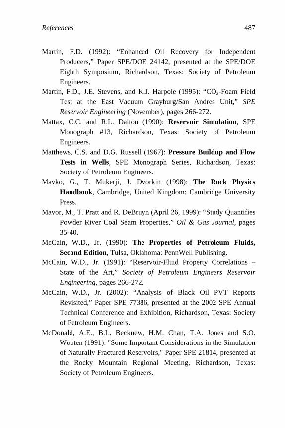
References 487
Martin, F.D. (1992): “Enhanced Oil Recovery for Independent Producers,” Paper SPE/DOE 24142, presented at the SPE/DOE Eighth Symposium, Richardson, Texas: Society of Petroleum Engineers.
Martin, F.D., J.E. Stevens, and K.J. Harpole (1995): “CO2-Foam Field Test at the East Vacuum Grayburg/San Andres Unit,” SPE
Reservoir Engineering (November), pages 266-272. Mattax, C.C. and R.L. Dalton (1990): Reservoir Simulation, SPE
Monograph #13, Richardson, Texas: Society of Petroleum Engineers.
Matthews, C.S. and D.G. Russell (1967): Pressure Buildup and Flow Tests in Wells, SPE Monograph Series, Richardson, Texas: Society of Petroleum Engineers.
Mavko, G., T. Mukerji, J. Dvorkin (1998): The Rock Physics Handbook, Cambridge, United Kingdom: Cambridge University Press.
Mavor, M., T. Pratt and R. DeBruyn (April 26, 1999): “Study Quantifies Powder River Coal Seam Properties,” Oil & Gas Journal, pages 35-40.
McCain, W.D., Jr. (1990): The Properties of Petroleum Fluids, Second Edition, Tulsa, Oklahoma: PennWell Publishing.
McCain, W.D., Jr. (1991): “Reservoir-Fluid Property Correlations – State of the Art,” Society of Petroleum Engineers Reservoir
Engineering, pages 266-272. McCain, W.D., Jr. (2002): “Analysis of Black Oil PVT Reports
Revisited,” Paper SPE 77386, presented at the 2002 SPE Annual Technical Conference and Exhibition, Richardson, Texas: Society of Petroleum Engineers.
McDonald, A.E., B.L. Becknew, H.M. Chan, T.A. Jones and S.O. Wooten (1991): "Some Important Considerations in the Simulation of Naturally Fractured Reservoirs," Paper SPE 21814, presented at the Rocky Mountain Regional Meeting, Richardson, Texas: Society of Petroleum Engineers.

488 Principles of Applied Reservoir Simulation
McIntosh, I., H. Salzew, and C. Christensen (1991): “The Challenge of Teamwork,” Paper CIM/AOSTRA 91-19, presented at the CIM/AOSTRA 1991 Technical Conference, Banff, Canada.
McKee, C.R., A.C. Bumb, and R.A. Koenig (March, 1988): "Stress-Dependent Permeability and Porosity of Coal and Other Geologic Formations," SPE Formation Evaluation, pages 81-91.
McQuillin, R., M. Bacon, and W. Barclay (1984): An Introduction to Seismic Interpretation, Houston: Gulf Publishing.
Medvin, E. and J. Rennie (July 1996): “Time to Depth: Where Geologists and Geophysicists Meet,” of Petroleum Technology, pages 595-599.
Mian, M.A. (1992): Petroleum Engineering Handbook for the Practicing Engineer, Volumes I and II, Tulsa, Oklahoma: PennWell Publishing.
Millheim, K.M. (1997): “Fields of Vision,” Journal of Petroleum
Technology, page 684. Mlacnik, M.J., and Z.E. Heinemann, (August 2003), “Using Well
Windows in Full-Field Reservoir Simulation,” SPE Reservoir
Evaluation and Engineering, pages 275-285. Mlacnik, M.J., A.W. Harrer, G.F. Heinemann, and Z.E. Heinemann
(March 2004): “State-of-the-Art of the Windowing Technique,” Journal of Canadian Petroleum Technology, pages 25-30.
Moses, P.L. (July 1986): “Engineering Applications of Phase Behavior of Crude Oil and Condensate Systems,” Journal of Petroleum
Technology, pages 715-723. Munka, M. and J. Pápay (2001): 4D Numerical Modeling of Petroleum
Reservoir Recovery, Budapest, Hungary: Akadémiai Kiadó. Murphy, W., A. Reisher, and K. Hsu (1993): “Modulus Decomposition
of Compressional and Shear Velocities in Sand Bodies,” Geophysics, Volume 58, pages 227-239.
Murtha, J.A. (1997): “Monte Carlo Simulation: Its Status and Future,”
Journal of Petroleum Technology, pages 361-373.
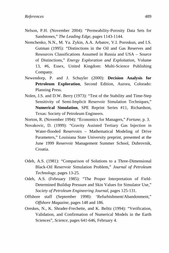
References 489
Nelson, P.H. (November 2004): “Permeability-Porosity Data Sets for Sandstones,” The Leading Edge, pages 1143-1144.
Nemchenko, N.N., M. Ya. Zykin, A.A. Arbatov, V.I. Poroskun, and I.S. Gutman (1995): “Distinctions in the Oil and Gas Reserves and Resources Classifications Assumed in Russia and USA – Source of Distinctions,” Energy Exploration and Exploitation, Volume 13, #6, Essex, United Kingdom: Multi-Science Publishing Company.
Newendorp, P. and J. Schuyler (2000): Decision Analysis for Petroleum Exploration, Second Edition, Aurora, Colorado: Planning Press.
Nolen, J.S. and D.W. Berry (1973): “Test of the Stability and Time-Step Sensitivity of Semi-Implicit Reservoir Simulation Techniques,” Numerical Simulation, SPE Reprint Series #11, Richardson, Texas: Society of Petroleum Engineers.
Norton, R. (November 1994): “Economics for Managers,” Fortune, p. 3. Novakovic, D. (1999): “Gravity Assisted Tertiary Gas Injection in
Water-flooded Reservoirs – Mathematical Modeling of Drive Parameters,” Louisiana State University preprint, presented at the June 1999 Reservoir Management Summer School, Dubrovnik, Croatia.
Odeh, A.S. (1981): “Comparison of Solutions to a Three-Dimensional
Black-Oil Reservoir Simulation Problem,” Journal of Petroleum
Technology, pages 13-25. Odeh, A.S. (February 1985): “The Proper Interpretation of Field-
Determined Buildup Pressure and Skin Values for Simulator Use,” Society of Petroleum Engineering Journal, pages 125-131.
Offshore staff (September 1998): ‘Refurbishment/Abandonment,” Offshore Magazine, pages 148 and 186.
Oreskes, N., K. Shrader-Frechette, and K. Belitz (1994): “Verification, Validation, and Confirmation of Numerical Models in the Earth Sciences”, Science, pages 641-646, February 4.
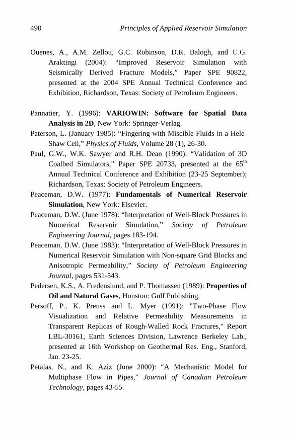
490 Principles of Applied Reservoir Simulation
Ouenes, A., A.M. Zellou, G.C. Robinson, D.R. Balogh, and U.G. Araktingi (2004): “Improved Reservoir Simulation with Seismically Derived Fracture Models,” Paper SPE 90822, presented at the 2004 SPE Annual Technical Conference and Exhibition, Richardson, Texas: Society of Petroleum Engineers.
Pannatier, Y. (1996): VARIOWIN: Software for Spatial Data
Analysis in 2D, New York: Springer-Verlag. Paterson, L. (January 1985): “Fingering with Miscible Fluids in a Hele-
Shaw Cell,” Physics of Fluids, Volume 28 (1), 26-30. Paul, G.W., W.K. Sawyer and R.H. Dean (1990): “Validation of 3D
Coalbed Simulators,” Paper SPE 20733, presented at the 65th Annual Technical Conference and Exhibition (23-25 September); Richardson, Texas: Society of Petroleum Engineers.
Peaceman, D.W. (1977): Fundamentals of Numerical Reservoir Simulation, New York: Elsevier.
Peaceman, D.W. (June 1978): “Interpretation of Well-Block Pressures in Numerical Reservoir Simulation,” Society of Petroleum
Engineering Journal, pages 183-194. Peaceman, D.W. (June 1983): “Interpretation of Well-Block Pressures in
Numerical Reservoir Simulation with Non-square Grid Blocks and Anisotropic Permeability,” Society of Petroleum Engineering
Journal, pages 531-543. Pedersen, K.S., A. Fredenslund, and P. Thomassen (1989): Properties of
Oil and Natural Gases, Houston: Gulf Publishing. Persoff, P., K. Preuss and L. Myer (1991): "Two-Phase Flow
Visualization and Relative Permeability Measurements in Transparent Replicas of Rough-Walled Rock Fractures," Report LBL-30161, Earth Sciences Division, Lawrence Berkeley Lab., presented at 16th Workshop on Geothermal Res. Eng., Stanford, Jan. 23-25.
Petalas, N., and K. Aziz (June 2000): “A Mechanistic Model for Multiphase Flow in Pipes,” Journal of Canadian Petroleum
Technology, pages 43-55.

References 491
Pletcher, J.L. (February 2002): “Improvements to Reservoir Material Balance Methods,” SPE Reservoir Evaluation & Engineering, pages 49-59.
Poettmann, F.H. and R.S. Thompson (1986): “Discussion of Engineering Applications of Phase Behavior of Crude Oil and Condensate Systems,” Journal of Petroleum Technology, pages 1263-1264.
Prats, M. (1982): Thermal Recovery, SPE Monograph Series, Richardson Texas: Society of Petroleum Engineers.
Preuss, K. and Y.W. Tsang (1990): "On Two-Phase Relative Permeability and Capillary Pressure of Rough-Walled Rock Fractures," Water Resources Research, Volume 26, pages 1915-1926.
Raghavan, R. and L.Y. Chin (August 2004): “Productivity Changes in
Reservoirs with Stress-Dependent Permeability,” SPE Reservoir
Evaluation & Engineering, pages 308-315. Raleigh, M. (Sept. 1991): ECLIPSE Newsletter, Houston: Schlumberger
GeoQuest. Rao, N.D. and M.G. Girard (January 1997): “A New Technique for
Reservoir Wettability Characterization,” Journal of Canadian
Petroleum Technology, Volume 35, pages 31-39. Raza, S.H. (1992): “Data Acquisition and Analysis for Efficient
Reservoir Management,” Journal of Petroleum Technology, pages 466-468.
Reiss, L.H. (1980): The Reservoir Engineering Aspects of Fractured Reservoirs, Houston: Gulf Publishing.
Reyes, L. and S.O. Osisanya (December 2002): “Empirical Correlation of Effective Stress Dependent Shale Rock Properties,” Journal of
Canadian Petroleum Technology, pages 47-53. Richardson, J.G., J.B. Sangree, and R.M. Sneider (1987a): “Applications
of Geophysics to Geologic Models and to Reservoir Descriptions,” Journal of Petroleum Technology, pages 753-755.
Richardson, J.G., J.B. Sangree and R.M. Sneider (1987b): “Introduction to Geologic Models,” Journal of Petroleum Technology (first of series), pages 401-403.

492 Principles of Applied Reservoir Simulation
Richardson, J.G. (February 1989): “Appraisal and Development of Reservoirs,” Geophysics: The Leading Edge of Exploration, pages 42 ff.
Rogers, R.E. (1994): Coalbed Methane: Principles and Practice, Englewood Cliffs, New Jersey: Prentice-Hall.
Rosenberg, D. U. von (1977): Methods for the Numerical Solution of Partial Differential Equations , Tulsa, Oklahoma: Farrar and Associates.
Rossini, C., F. Brega, L. Piro, M. Rovellini, and G. Spotti (November 1994): “Combined Geostatistical and Dynamic Simulations for Developing a Reservoir Management Strategy: A Case History,” Journal of Petroleum Technology, pages 979-985.
Ruijtenberg, P.A., R. Buchanan, and P. Marke (1990): “Three-Dimensional Data Improve Reservoir Mapping,” Journal of
Petroleum Technology, pages 22-25, 59-61. Sabet, M.A. (1991): Well Test Analysis, Houston: Gulf Publishing. Saleri, N.G. (1993): “Reservoir Performance Forecasting: Acceleration
by Parallel Planning,” Journal of Petroleum Technology, pages 652-657.
Saleri, N.G. (2002): “’Learning’ Reservoirs: Adapting to Disruptive Technologies,” Journal of Petroleum Technology, pages 57-60.
Saleri, N.G. (2005): “Reservoir Management Tenets: Why They Matter to Sustainable Supplies,” Journal of Petroleum Technology, pages 28-30.
Saleri, N.G., R.M. Toronyi, and D.E. Snyder (1992): “Data and Data Hierarchy,” Journal of Petroleum Technology, pages 1286-1293.
Satter, A. and G. Thakur (1994): Integrated Petroleum Reservoir Management, Tulsa: PennWell Publishing.
Satter, A., J.E. Varnon, and M.T. Hoang (1994): “Integrated Reservoir Management,” Journal of Petroleum Technology, pages 1057-1064.
Sawyer, W.K. and J.C. Mercer (August 1978): “Applied Simulation Techniques for Energy Recovery,” Department of Energy Report METC/RI-78/9, Morgantown, West Virginia.
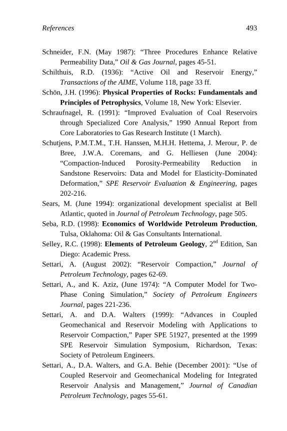
References 493
Schneider, F.N. (May 1987): “Three Procedures Enhance Relative Permeability Data,” Oil & Gas Journal, pages 45-51.
Schilthuis, R.D. (1936): “Active Oil and Reservoir Energy,” Transactions of the AIME, Volume 118, page 33 ff.
Schön, J.H. (1996): Physical Properties of Rocks: Fundamentals and Principles of Petrophysics, Volume 18, New York: Elsevier.
Schraufnagel, R. (1991): “Improved Evaluation of Coal Reservoirs through Specialized Core Analysis,” 1990 Annual Report from Core Laboratories to Gas Research Institute (1 March).
Schutjens, P.M.T.M., T.H. Hanssen, M.H.H. Hettema, J. Merour, P. de Bree, J.W.A. Coremans, and G. Helliesen (June 2004): “Compaction-Induced Porosity-Permeability Reduction in Sandstone Reservoirs: Data and Model for Elasticity-Dominated Deformation,” SPE Reservoir Evaluation & Engineering, pages 202-216.
Sears, M. (June 1994): organizational development specialist at Bell Atlantic, quoted in Journal of Petroleum Technology, page 505.
Seba, R.D. (1998): Economics of Worldwide Petroleum Production, Tulsa, Oklahoma: Oil & Gas Consultants International.
Selley, R.C. (1998): Elements of Petroleum Geology, 2nd Edition, San Diego: Academic Press.
Settari, A. (August 2002): “Reservoir Compaction,” Journal of
Petroleum Technology, pages 62-69. Settari, A., and K. Aziz, (June 1974): “A Computer Model for Two-
Phase Coning Simulation,” Society of Petroleum Engineers
Journal, pages 221-236. Settari, A. and D.A. Walters (1999): “Advances in Coupled
Geomechanical and Reservoir Modeling with Applications to Reservoir Compaction,” Paper SPE 51927, presented at the 1999 SPE Reservoir Simulation Symposium, Richardson, Texas: Society of Petroleum Engineers.
Settari, A., D.A. Walters, and G.A. Behie (December 2001): “Use of Coupled Reservoir and Geomechanical Modeling for Integrated Reservoir Analysis and Management,” Journal of Canadian
Petroleum Technology, pages 55-61.
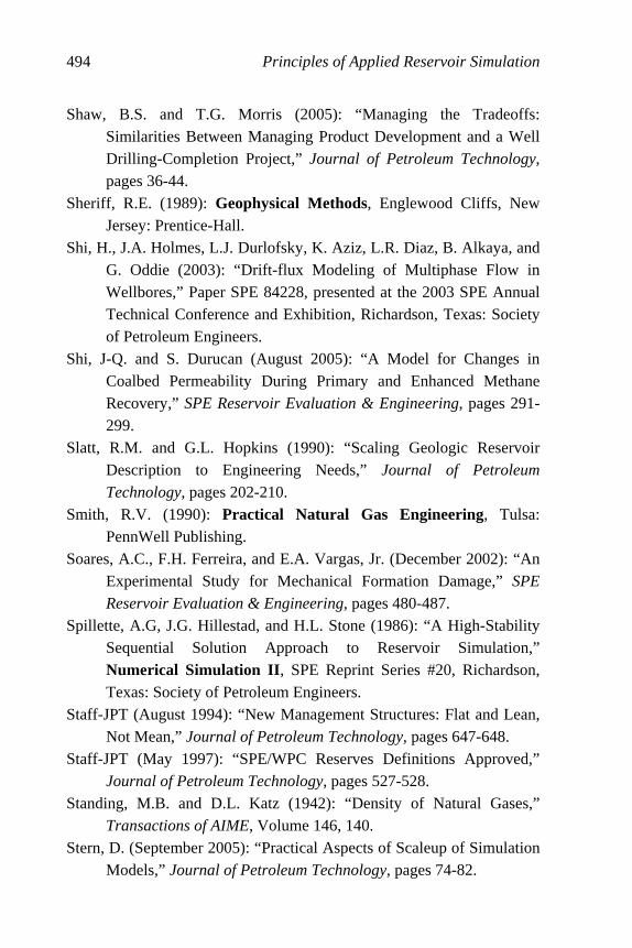
494 Principles of Applied Reservoir Simulation
Shaw, B.S. and T.G. Morris (2005): “Managing the Tradeoffs: Similarities Between Managing Product Development and a Well Drilling-Completion Project,” Journal of Petroleum Technology, pages 36-44.
Sheriff, R.E. (1989): Geophysical Methods, Englewood Cliffs, New Jersey: Prentice-Hall.
Shi, H., J.A. Holmes, L.J. Durlofsky, K. Aziz, L.R. Diaz, B. Alkaya, and G. Oddie (2003): “Drift-flux Modeling of Multiphase Flow in Wellbores,” Paper SPE 84228, presented at the 2003 SPE Annual Technical Conference and Exhibition, Richardson, Texas: Society of Petroleum Engineers.
Shi, J-Q. and S. Durucan (August 2005): “A Model for Changes in Coalbed Permeability During Primary and Enhanced Methane Recovery,” SPE Reservoir Evaluation & Engineering, pages 291-299.
Slatt, R.M. and G.L. Hopkins (1990): “Scaling Geologic Reservoir Description to Engineering Needs,” Journal of Petroleum
Technology, pages 202-210. Smith, R.V. (1990): Practical Natural Gas Engineering, Tulsa:
PennWell Publishing. Soares, A.C., F.H. Ferreira, and E.A. Vargas, Jr. (December 2002): “An
Experimental Study for Mechanical Formation Damage,” SPE
Reservoir Evaluation & Engineering, pages 480-487. Spillette, A.G, J.G. Hillestad, and H.L. Stone (1986): “A High-Stability
Sequential Solution Approach to Reservoir Simulation,” Numerical Simulation II , SPE Reprint Series #20, Richardson, Texas: Society of Petroleum Engineers.
Staff-JPT (August 1994): “New Management Structures: Flat and Lean, Not Mean,” Journal of Petroleum Technology, pages 647-648.
Staff-JPT (May 1997): “SPE/WPC Reserves Definitions Approved,” Journal of Petroleum Technology, pages 527-528.
Standing, M.B. and D.L. Katz (1942): “Density of Natural Gases,” Transactions of AIME, Volume 146, 140.
Stern, D. (September 2005): “Practical Aspects of Scaleup of Simulation Models,” Journal of Petroleum Technology, pages 74-82.
References 495
Stolz, A-K. and R.M. Graves (2003): “Sensitivity Study of Flow Unit Definition by Use of Reservoir Simulation,” Paper SPE 84277, presented at the 2003 SPE Annual Technical Conference and Exhibition, Richardson, Texas: Society of Petroleum Engineers.
Stone, H.L. (October-December 1973): “Estimation of Three-Phase Relative Permeability and Residual Oil Data,” Journal of
Canadian Petroleum Technology, pages 53 ff. Taber, J.J. and F.D. Martin (1983): “Technical Screening Guides for the
Enhanced Recovery of Oil,” Paper SPE 12069, presented at the 58th Annual Technical Conference and Exhibition, Richardson, Texas: Society of Petroleum Engineers.
Taber, J.J., F.D. Martin and R.S. Seright (1997a): “EOR Screening Criteria Revisited: Part 1 – Introduction to Screening Criteria and Enhanced Recovery Field Projects,” SPE Reservoir Evaluation
and Engineering, pages 189-198. Taber, J.J., F.D. Martin and R.S. Seright (1997b): “EOR Screening
Criteria Revisited: Part 2 – Applications and Implications of Oil Prices,” SPE Reservoir Evaluation and Engineering, pages 199-205.
Taggart, I.J., E. Soedarmo, and L. Paterson (1995): “Limitations in the Use of Pseudofunctions for Up-Scaling Reservoir Simulation Models,” Paper SPE 29126, presented at the 13th Society of Petroleum Engineers Symposium on Reservoir Simulation, Richardson, Texas: Society of Petroleum Engineers.
Tearpock, D.J., R.E. Bischke and L.G. Walker (2002): Applied Subsurface Geological Mapping with Structural Methods, Englewood Cliffs, New Jersey: Prentice Hall.
Tearpock, D.J. and J.C. Brenneke (2001): “Multidisciplinary teams, integrated software for shared-earth modeling key E&P success,” Oil & Gas Journal, pages 84-88 (10 December).
Teeuw, D. (Sept. 1971): “Prediction of Formation Compaction from Laboratory Compressibility Data,” Society of Petroleum
Engineering Journal, pages 263-271.
496 Principles of Applied Reservoir Simulation
Tek, M.R. (1996): Natural Gas Storage Underground: Inventory and Deliverability , Tulsa: PennWell Publishing.
Telford, W.M., L.P. Geldart, R.E. Sheriff, and D.A. Keys (1976): Applied Geophysics, Cambridge: Cambridge University Press.
Thakur, G.C. (1996): “What Is Reservoir Management?” Journal of
Petroleum Technology, pages 520-525. Thomas, F.B., E. Shtepani, D. Imer, and D.B. Bennion (January 2002):
“How Many Pseudo-Components are Needed to Model Phase Behaviour?” Journal of Canadian Petroleum Technology, pages 48-54.
Thomas, G.W. (1982): Principles of Hydrocarbon Reservoir Simulation, Boston: International Human Resources Development Corporation.
Thomas, L. K., W. B. Lumkin and G. M. Reheis (1976): “Reservoir Simulation of Variable Bubble Point Problems,” Society of
Petroleum Engineers Journal, pages 10-16. Thompson, R.S. and J.D. Wright (1985): Oil Property Evaluation ,
Second Edition, Golden, Colorado: Thompson-Wright Associates. Tiab, D. and E.C. Donaldson (2003): Petrophysics, Second Edition,
Boston: Elsevier. Tippee, Bob (1998): “Collaborative Effort Seeks Computing Platform
for Shared Earth Modeling,” Oil & Gas Journal, pages 58-62 (30 November).
Tobias, S. (1998): “From G&G to S&S: Watershed Changes in Exploration-Development Work Flow,” Oil and Gas Journal, pages 38-47 (30 November).
Todd, M.R. and W.J. Longstaff (1972): “The Development, Testing and Application of a Numerical Simulator for Predicting Miscible Flood Performance,” Journal of Petroleum Technology, pages 874-882.
Todd, M.R., P.M. Odell, and G.J. Hiraski (December 1972): “Methods for Increased Accuracy in Numerical Reservoir Simulators,” Society of Petroleum Engineering Journal, pages 515-530.
Toronyi, R.M. and N.G. Saleri (1988): “Engineering Control in Reservoir Simulation,” Paper SPE 17937, presented at the 1988

References 497
Society of Petroleum Engineers Annual Technical Conference and Exhibition, Richardson, Texas: Society of Petroleum Engineers.
Towler, B.F. (2002): Fundamental Principles of Reservoir Engineering, Richardson, Texas: Society of Petroleum Engineers.
Tran, D., A. Settari, and L. Nghiem (2002): “New Iterative Coupling Between a Reservoir Simulator and a Geomechanics Module,” SPE/ISRM 78192, presented at the 2002 SPE/ISRM Rock Mechanics Conference, Irving, Texas (23-25 October).
Turner, R.G., M.G. Hubbard, and A.E. Dukler (November 1969): “Analysis and Prediction of Minimum Flow Rate for the Continuous Removal of Liquids from Gas Wells,” Journal of
Petroleum Technology, pages 1475-1482. Uland, M.J., S.W. Tinker, and D.H. Caldwell (1997): “3-D Reservoir
Characterization for Improved Reservoir Management,” paper presented at the 1997 Society of Petroleum Engineers’ 10th Middle East Oil Show and Conference, Bahrain (March 15-18).
Verma, S. and K. Aziz (1997): “A Control Volume Scheme for Flexible
Grids in Reservoir Simulation,” Paper SPE 37999, presented at the 1997 Society of Petroleum Engineers Reservoir Simulation Symposium, Richardson, Texas: Society of Petroleum Engineers.
Vogel, J.V. (January 1968): “Inflow Performance Relationships for Solution-Gas Drive Wells,” Journal of Petroleum Technology, page 83 ff.
Waal, H. de, and R. Calvert (2003): “Overview of Global 4D Seismic
Implementation Strategy,” Petroleum Geosciences, Volume 9, pages 1-6.
Wade, J.M. and V.I. Fryer (1997): “A Case Study of a Multi-Disciplinary Asset Management Team, with Special Emphasis on the Impact on Performance and Business Growth,” Paper SPE 38823, presented at the 1997 Society of Petroleum Engineers Annual Technical Conference and Exhibition, Richardson, Texas: Society of Petroleum Engineers.

498 Principles of Applied Reservoir Simulation
Walsh, M.P. and L.W. Lake (2003): A Generalized Approach to Primary Hydrocarbon Recovery, Amsterdam: Elsevier.
Wang, F.P., J. Dai, and C. Kerans (1998): “Modeling Dolomitized Carbonate-Ramp Reservoirs: A Case Study of the Seminole San Andres Unit – Part II, Seismic Modeling, Reservoir Geostatistics, and Reservoir Simulation,” Geophysics, Volume 63, pages 1876-1884.
Wang, P. and G.A. Pope (July 2001): “Proper use of Equations of State for Compositional Reservoir Simulation,” Journal of Petroleum
Technology, pages 74-81. Wang, Z. (2000): “Dynamic versus Static Elastic Properties of Reservoir
Rocks,” in Seismic and Acoustic Velocities in Reservoir Rocks, Volume 3, Recent Developments, edited by Z. Wang and A. Nur, Tulsa, Oklahoma: Society of Exploration Geophysicists.
Watkins, R. W. (1982): “The Development and Testing of a Sequential, Semi-Implicit Four Component Reservoir Simulator,” Paper SPE 10513, Richardson, Texas: Society of Petroleum Engineers.
Wattenbarger, R.A. (July 2002): “Trends in Tight Gas Sand Production,” Journal of Canadian Petroleum Technology, pages 17-20.
Weinstein, H.G., J.E. Chappelear, and J.S. Nolen (1986): “Second Comparative Solution Project: A Three-Phase Coning Study,” Journal of Petroleum Technology, pages 345-353.
Westlake, D.W.S. (1999): “Bioremediation, Regulatory Agencies, and Public Acceptance of this Technology,” Journal of Canadian
Petroleum Technology, Volume 38, pages 48-50. Whitson, C.H. and M.R. Brulé (2000): Phase Behavior, SPE
Monograph Series, Richardson, Texas: Society of Petroleum Engineers.
Whittaker, M. (1999): “Emerging ‘triple bottom line’ model for industry weighs environmental, economic, and social considerations,” Oil
& Gas Journal, pages 23-28 (20 December). Wiggins, M.L. and R.A. Startzman (1990): “An Approach to Reservoir
Management,” Paper SPE 20747, presented at the 65th Annual Technical Conference And Exhibition of the Society of Petroleum Engineers, Richardson, Texas: Society of Petroleum Engineers.

References 499
Wigley, T.M.L., R. Richels, and J.A. Edmonds (1996): “Economic and environmental choices in the stabilization of atmospheric CO2
concentrations,” Nature (18 January), pages 240-243. Wilhite, G.P. (1986): Waterflooding, SPE Textbook Series Volume 3,
Richardson, Texas: Society of Petroleum Engineers. Wilkinson, A.J. (September 1997): “Improving Risk-Based
Communications and Decision Making,” Journal of Petroleum
Technology, pages 936-943. Williamson, A.E. and J.E. Chappelear (June 1981): “Representing Wells
in Numerical Reservoir Simulation: Part I – Theory,” Society of
Petroleum Engineers Journal, pages 323-338; and “Part II – Implementation,” Society of Petroleum Engineers Journal, pages 339-344.
Winterfeld, P.H. (June 1989): “Simulation of Pressure Buildup in a Multiphase Wellbore-Reservoir System,” SPE Formation
Evaluation, pages 247-252. Worthington, P.F. and L. Cosentino (August 2005): “The Role of Cutoffs
in Integrated Reservoir Studies,” SPE Reservoir Evaluation &
Engineering, pages 276-290. Yale, D.P. (2002): “Coupled Geomechanics-Fluid Flow Modeling:
Effects of Plasticity and Permeability Alteration,” SPE/ISRM 78202, presented at the 2002 SPE/ISRM Rock Mechanics Conference, Richardson, Texas: Society of Petroleum Engineers.
Young, L.C. (1984): “A Study of Spatial Approximations for Simulating Fluid Displacements in Petroleum Reservoirs,” Computer Methods in Applied Mechanics and Engineering, New York: Elsevier, pages 3-46.
Zuber, N., and J.A. Findlay, (1965): “Average Volumetric Concentration
in Two-Phase Flow Systems,” Journal of Heat Transfer, Transactions ASME, Volume 87, pages 453-468.

500
INDEX
3
3DVIEW introduced 11
4
4-D seismic 228
A
absolute permeability 37, 39, 42, 62, 153, 171, 173
acoustic impedance 215-217, 223, 227, 230, 391, 448
analytic aquifer 205, 206, 209, 371, 386, 391, 442
anistropic permeability 263 anisotropy 259, 262, 263, 271 aquifer influx 115, 205, 206,
209, 361, 365-367, 370, 371, 386, 390, 391, 442, 448
aquifer model 206, 368, 371 Archie's equation 236 areal model 208, 301, 330 areal sweep efficiency defined
80
B
barrier 25, 44, 241, 245, 385 base case 189, 323, 374, 386,
387 baseline 133, 189 bioremediation 129 Biot coefficient 269 black oil model 309, 310 black oil simulator 9, 144, 148,
151, 152, 154, 155, 271, 273, 309, 310, 347
block centered 394 bottomhole pressure 201, 380,
381 boundaries 97, 169, 172, 218,
238-240, 283, 286, 331, 352, 361, 369
boundary conditions 58, 66, 67, 69, 110, 172, 283
Brent Spar 130 bubble point pressure tracking
314 Buckley-Leverett 51, 54, 55, 57,
60, 62, 63, 66, 166, 184, 188
Index 501
buildup 196, 239, 240, 242, 382 bulk density 216, 217, 223, 224,
226, 231, 235 bulk modulus 113, 139, 223-
226, 230-232, 274, 415-419 bulk volume 15, 45, 255, 264,
326, 364, 397
C
calibration 189, 351 capillary pressure correction 35 capillary pressure defined 30,
320 capillary tube model 264 carbonate 44, 45, 135, 234, 237,
256, 258, 259, 268 Carter-Tracy 206 Cartesian 15, 156, 242, 252,
328, 330, 331, 336, 391 cash flow 2, 119-121, 126, 127,
189, 373, 386 C-D equation 57, 58 centerpoint 283 chemical flood 103 climate change 131 coal gas 9, 106, 110, 111, 134,
151, 391, 443, 444 coalbed methane 9, 106-108,
112, 115, 259 coarse grid 284 combination log 236 combustion 131 compaction 107, 133, 134, 140,
172, 269-273, 276, 277, 280 completion 86, 91, 92, 172, 180,
192, 248, 352, 354, 357, 391, 446
compositional simulator 149- 151, 154, 155, 172, 205, 309, 310
compressibility factor 309 compressional velocity 113,
216, 217, 223, 224, 231, 232, 448
computer mapping 16, 286, 287 computer program 1, 3, 10, 286,
287, 333 concentration 57, 58, 64, 131,
142, 144, 146, 166, 359, 434, 435
conceptual model 282, 283, 330, 358, 375, 379
condensate 151, 154, 155, 305, 306-308, 310, 324
consensus modeling 3 conservation laws 143, 190 conservation of mass 16, 52,
141, 143, 190, 204 constraint 146, 178-181, 238,
294, 296, 298, 320, 338, 341, 348, 353, 361, 377, 386, 437, 454, 458
contact angle defined 29 continuity equation 65, 141, 143 contour 54, 219, 220, 285, 286 contouring 219, 283, 301 convection 51, 57, 149, 150,
169 core analysis 15, 211, 244, 256,
352 core flood 93, 328, 357, 369 core permeability 298 corner point 331-334 corporate 2, 125, 158, 378 countercurrent 201 cricondentherm 306 crossplot 220, 237, 250, 265,
266, 291, 298 cross-section model 49, 91, 330 cubic equation 309 cutoff 54, 236

502 Principles of Applied Reservoir Simulation
cylindrical 234, 264, 278, 328, 330, 331
D
data acquisition 222, 353 data processing 215 data quality 357 data sampling 211 datum 242, 245, 260, 400, 420,
436 decision making 1, 7, 125, 127,
128, 362 density gradient 31, 32, 49 desorption pressure 111, 444 deterministic 289, 290, 297 deviated well 9, 139 dew point 154, 306, 310, 324 diagonal grid 335 differential equations 69 differential liberation 312, 313,
347 differentials 177-79 diffusion 57, 106, 110, 112, 444 digitize 284, 285, 358 dimensionality 154, 156 dipping 42, 68, 70, 72, 98, 99,
260, 321, 328, 332, 341 direct solution 441 directional permeability 259 discount rate defined 121 discretize 163 dispersion 51, 57, 62, 149, 150,
166-168, 184, 185 displacement efficiency defined
78-79 dissolved gas drive 98 double displacement process
104 downdip 104, 370, 387
drawdown 208, 239, 324, 354, 360
drill stem test, 238, 313, 344 drilling technology 84 dry gas 154, 155, 306-308 dual continuum 91 Dykstra-Parsons 87, 88, 9-95 dynamic viscosity 193, 194, 208
E
economic forecast 2, 119 economic measures 121, 125 economic recovery 2 economics 78, 117, 129 economies 132 effective permeability 37, 105,
173, 175, 380 effective porosity 256 elevation 32, 33, 284, 320, 337,
338, 341, 390, 420 endpoints 357 energy balance 132, 151, 194,
195 Enhanced Oil Recovery 102,
126 environment 8, 44, 85, 117, 126,
128, 130, 134, 210, 222, 233, 249, 258, 304
EOR 97, 102, 103, 105, 115, 126
equation of state 309, 315 equilibration 18, 31, 144, 260,
310, 327, 337, 435 equivalent height defined 32 equivalent radius 254, 382, 383 explicit pressure 178-181, 454,
455, 457, 458 explicit saturation 163, 330 exponential decline 21 extended reach drilling 84, 85

Index 503
F
facilities 124, 190-192, 199, 310, 312, 313, 377
falloff 239 fault 172, 237, 241, 284, 286,
297, 331, 342, 345, 352, 363, 370, 375
fence diagram 236 Fick 57, 110 fine grid 59, 60, 284 finger growth 72 fingering 59 finite difference 58, 62, 111,
162, 163, 166, 168, 169, 171, 205, 206, 331, 335, 336, 379, 388
finite element 331 five-point 336 five-spot 81, 88, 93, 94, 335 flash 312, 313, 347, 349 flexible grid 331 flow chart 164, 165 flow pattern 199 flow regimes 197, 198 flow unit 233, 244-247, 250,
252, 254, 353 fluid allocation 176 fluid compressibility 139, 225,
226, 353 fluid contacts 34, 284, 320, 321,
323, 327, 352, 357 fluid density 193, 208, 224, 235 fluid movement 64, 328 fluid properties 60, 197, 205,
215, 228, 274, 309, 312-314, 346, 353, 362, 388
fluid sampling 313, 314 fluid type 78, 154-56, 234, 306-
309
flux 141, 142, 144, 159, 200, 204, 283, 361
forecasting 373, 378 fossil fuel 131 fractional flow 27, 38, 40, 41,
42, 43, 51-56, 62, 63, 66 fracture capillary pressure 46 fracture gradient 269, 270 fracture permeability 45, 46 fracture porosity 63 fracture relative permeability
46, 47, 93 fractured reservoir 45-46, 49,
83, 91, 156, 181-183, 186, 259, 320
free water level defined 33 friction factor 196 frontal advance 52, 54, 55, 68,
70, 72, 73, 167, 185, 335 frontal stability defined 65 full field model, 282, 284, 297,
329, 351 full field model 282, 283 fully implicit 164-168, 170,
172, 182-185, 330
G
gamma ray 234, 235, 237 gas cap 12, 18, 19, 24, 26, 46,
98, 321, 324, 349, 357 gas compressibility 20, 22, 23,
315 gas density 338 gas drive 98 gas formation volume factor 14,
26, 145, 310, 312, 315, 325, 426
gas hydrate 107, 108 gas storage reservoir defined
100
504 Principles of Applied Reservoir Simulation
gas viscosity 44, 310, 315, 325, 426
gas-oil capillary pressure 44, 338, 411
gas-oil contact 35, 321, 337, 357, 436
gas-oil ratio 14, 26, 86, 89, 155, 164, 180, 191, 275, 306, 313, 314, 325, 347, 350, 355, 390, 425, 439
gas-oil relative permeability 319 Gassmann 226 gas-water 26, 107, 108, 151,
164, 177, 321, 329, 339, 353, 425, 437
geologic model 3, 156, 247, 290, 291, 343, 358
geology 8, 156, 215, 241, 290, 364
geomechanical model 268, 271 geomechanics 133, 270 geometry 52, 68, 83, 156, 194,
236, 264, 331-333, 339, 394 geophysics 8, 213-215, 222,
241, 289 geostatistical modeling 291 geostatistics 287, 289, 290, 296,
297, 299, 300, 358 geosteering 85, 86 Giga Scale 210, 211, 213, 233 global warming 131, 132 gradient 31, 49, 199, 225, 260,
283, 305, 381, 440, 441 grain density 225, 274, 415-417,
419 grain modulus 225, 230, 274 grain volume 255 gravity 109 gravity drainage 46, 98, 104 gravity segregated 339, 435
gravity segregation 18, 99, 337, 349
greenhouse effect defined 131 greenhouse gases 131, 132 grid orientation 166, 328, 334-
336 grid preparation 283, 331 grid size 282, 394, 398 gridblock pressure 164, 206,
242, 243, 314, 324, 382, 383, 431
gridblock size 167, 230, 254, 390, 396
gross thickness 15, 24, 94, 248, 284, 298, 326, 342, 394, 395, 397, 399
H
hand-drawn 297, 298 harmonic decline 21 heavy oil 154, 306 heterogeneous 9, 84, 91, 94,
219, 250, 259, 260, 262 hierarchy of uncertainty 357 historical data 168, 189, 363,
386, 387 history matching evaluation 359 history matching limitations 361 history matching parameters
357 history matching stage 343, 351 history matching strategies 354 homogeneous 59, 88, 156, 200,
234, 259, 262, 263 Honarpour 317, 368 horizontal permeability 175,
228, 240, 259, 274, 329, 382 horizontal well 83, 175, 176,
192, 202, 375, 451 Horner plot 242

Index 505
hydraulic radius model 264 hyperbolic decline 21 hysteresis 38, 151
I
IFLO coal gas model 110 IFLO introduced 8 IFLO flow equations 151 IFLO fluid model 314 IFLO geomechanical model 268 IFLO initialization model 337 IFLO petrophysical model 223 IFLO productivity index 174 IFLO solution procedure 168 IFLO three-phase relative
permeability 319 IFLO transmissibility 171 IFLO volumetrics 15 IFLO well model 173 immiscible 27, 29, 30, 33, 43,
44, 51, 52, 57, 60, 66, 101, 102, 104, 137, 320, 322
IMPES 163-168, 170, 172, 182-185, 330, 384, 390
implicit 163, 165, 167, 179, 204, 388
implicit pressure 163, 179, 388 Improved Oil Recovery 102 incompressible 51, 52, 60, 66,
86, 112, 196, 366 infill drilling 83, 84, 102, 135 inflation rate 122 inflow performance relationship
202, 204 initialization data 388, 390, 393 integrated flow model, 8, 113,
151, 223, 271, 272 intelligent well 86 interfacial tension 27, 28, 31,
35, 57, 102, 104
interference testing 352 interstitial velocity 63 inverse distance weighting 287,
288 inverse problem 189, 361, 362 investment 1, 120-122, 125-128,
130, 369, 375 IPR 202, 203 irreducible 33, 55, 61, 62, 92,
319-321, 324, 337, 369, 410, 411, 438
isothermal 8, 18, 144, 151, 154, 190, 312, 315, 388
isotropic 174, 228, 234, 244, 260, 262, 263, 334, 382
isotropy 244, 259
J
Jacobian 163 Joshi 175, 202 J-function 36, 47
K
kinematic viscosity 208 Klinkenberg 106 Kozeny-Carman 265 Krige 293 kriging 289, 293-295, 302 kriging accuracy 295 Kyoto Protocol 132
L
laboratory measurements 30, 35, 230, 313, 316, 347
laboratory measurements 256, 316
lag 57, 292-294, 301 Lagrange multiplier 294-296 Langmuir isotherm defined 110
506 Principles of Applied Reservoir Simulation
layer cake 329, 400 linear stability analysis 70 line-drive 82, 83, 87, 91 liquid loading 201 LIT gas well analysis 454, 458 LIT method 179 local grid refinement (LGR)
156, 331 logging 233, 256 log-normal 46, 47, 87, 93, 250
M
Macleod-Sugden 28, 35 Macro Scale 211, 316 mapping 282, 284-287, 298 mass balance 52, 143 mass conservation 142, 143,
146, 150 material balance equation 16-
20, 22, 24, 99, 169, 365-367 material balance error 161, 164,
183, 186, 390, 392, 438, 441 matrix equation 58, 163, 180,
295 matrix material 415 matrix permeability 45, 259 matrix rock 45, 63 matrix-fracture 46, 63 mega scale 211, 212, 233, 234,
238 megacell 332 midpoint 160, 225, 321, 322,
337, 338, 390, 391 miscibility 104, 136, 137, 411,
430, 431 miscible 57, 104, 137, 152, 429,
430 Micro Scale 211, 258, 316 microbial 102, 105, 115
mobility defined 39 mobility ratio 39, 63, 67, 72-76,
86-88, 103, 104 model calibration 189, 361, 373,
374 model initialization 320, 327,
390 modified Lorenz plot 245 molar conservation 150 mole fraction 28, 150, 427 molecular weight 28, 29, 103,
307, 308, 427, 428 momentum, 143, 144, 190, 193 multidisciplinary 7, 299 multilateral well 84, 85 multiphase flow 27, 197-200,
202, 204, 317, 318 multivariable 170, 191, 375,
376
N
naturally fractured 44-46, 49, 91, 156, 182, 183, 186, 259
near wellbore 156, 358 net pay 207 net present value 120, 121, 125,
128 net thickness defined 16 net-to-gross 15, 24, 94, 160,
284, 298, 326, 342, 397 Newton-Raphson 163, 164, 170,
441 nine-point 336 no-flow 172, 241, 345 nonunique 189, 362, 379 nonwetting 31, 32, 33, 34 normal distribution 95, 119, 137 NOx 131 nugget 293, 295, 301
Index 507
numerical aquifer 205 numerical dispersion defined
166 numerical oscillations 183
O
Ockham's Razor 5, 154, 155, 157, 330
oil compressibility 312 oil density 337, 338, 381, 429 oil formation volume factor 14,
79, 94, 310, 313, 324, 347, 364, 424, 425, 430
oil productive capacity 219 oil property correction 312 oil viscosity 42, 48, 62, 72, 73,
76, 310, 325, 349, 424, 425, 430
oil-water capillary pressure 43, 410
oil-water relative permeability 75, 76
oil-wet 30
P
parachor 28, 48 parallel grid 335 parallel processor 332 parallelograms 333 partial differential equations
162, 204 pattern 59, 78, 81-84, 86-88,
102, 103, 135, 189, 197, 199, 200, 273, 334, 335, 379
payout 120, 121, 125 Peaceman 3, 58, 162, 174, 175,
354, 382 Peaceman's pressure correction
242, 243, 253, 254, 382
PEBI 332
performance data 4, 391 performance predictions 187,
373, 376, 378, 379 permeability and Darcy's Law
257 permeability anistropy 263 permeability heterogeneity 262 permeability tensor 150, 261,
262, 336 petrophysical model 8, 9, 215,
223, 357 petrophysics 8, 241 phase behavior 305, 310 phase envelope 305-307 phase potential defined 153, 260 pipe roughness 196 piston-like displacement 56, 57,
62, 65, 66, 74, 166 Poisson's equation 65 Poisson's ratio 113, 133, 139,
268, 269, 274, 391, 415, 422-424, 449
pore radius 32, 48 pore size 259 pore volume defined 15 porosity defined 255 porosity-permeability crossplot
265 porous medium 47, 51, 59, 65,
66, 149, 223, 236, 255, 256, 258, 262, 265
prediction process 373 prediction stage 157, 351, 373,
374, 386 prediction validity 378 pressure correction, 242, 355 pressure depletion 24, 100, 101,
107, 114, 133, 134, 139, 201, 355
508 Principles of Applied Reservoir Simulation
pressure gradient 34, 40, 98, 106, 150, 153, 195, 196, 199, 209, 260, 338, 339, 358, 381, 420
pressure initialization 435 pressure maintenance 101, 133 pressure transient testing 237 price forecast 2, 189, 377, 386 primary porosity 237, 256 primary production 98, 99, 101 primary recovery 95 principal axes 262, 263, 336 producer: injector ratio 83 production stages 97 productivity index 173, 179,
207, 357, 373, 380 profit-to-investment ratio
defined 121 pseudocomponent 151, 152 pseudoization 329 pseudopressure 179, 315, 316 pseudorelative permeability
330, 358 P-T diagram 305, 307 PVT region 390
Q
quasistationary 174, 380
R
radial coordinates 156, 207 radial flow 173, 240, 243, 383 radius of investigation 240, 241,
345 rate constraint, 176, 451 rate of return 120, 123-125 real options analysis 127 realizations 290, 291, 297-300,
327
reasonableness 5, 361 recovery efficiency 16, 78, 80,
81, 84, 94, 99, 101, 307 recurrent data 388, 391, 446,
447 reflection coefficient 216, 217,
227, 230, 391, 449 regression 28, 226, 227, 266,
289, 291, 310, 375, 376 relative mobility defined 39 relative permeability defined 37 relative permeability, saturation
exponent method 317 reliability 211, 357, 360 repeat formation test 238, 323 representative elementary
volume 143, 244, 247 reserves 108, 117-119, 123,
137, 378 reservoir architecture 144, 156,
211, 233, 332, 385 reservoir characterization 84,
135, 187, 211, 217, 221, 228, 284, 289, 296, 327
reservoir depletion 98 reservoir depth 105 reservoir description 111, 155,
189, 210, 388 reservoir engineering 9, 10, 123,
143, 187, 305, 362, 379 reservoir geophysics 213, 214,
219, 221, 289 reservoir geophysics 213, 220 reservoir management
constraints 348, 386, 387 reservoir management modeling
system 190 reservoir management objective
2, 86, 341, 362 reservoir scales 210

Index 509
reservoir simulation 1, 91, 123, 143, 144, 188, 190, 191, 200, 203, 286, 341, 378
reservoir simulation study 188 reservoir structure 11, 151, 213,
369 resistivity 234, 235, 236 restart 436 restored state 37 revenue 120, 121, 122, 124,
128, 377 Reynolds number 193, 194,
196, 208 risk 127, 189, 210, 298, 375 risk analysis 127, 375 robustness 166 rock compressibility 112, 160,
271, 274, 358, 359, 365, 426, 428
rock properties and fluid flow 255
rock quality 219, 221, 258 rock region 353, 407, 408, 436,
438 rock-fluid interaction 151, 274
S
sandstone 24, 44, 105, 111-113, 217, 255, 256, 259, 278, 297, 343, 368
saturated 111, 154, 158, 170, 236, 278, 304, 309, 310, 314, 324, 425, 432, 444
saturated bulk modulus 223, 226
saturation distribution 54, 172, 228, 339, 391
saturation pressure 310 scaleup 244, 286 Schilthuis material balance 17
second contact water displacement process 104
secondary porosity 237, 256, 259
secondary production 101 secondary recovery 101, 102,
191 sector model, 282, 361 seismic history matching 356 seismic line 342 seismic method 221 seismic trace 214, 215, 217 seismic velocity 215, 449 seismic velocity model 215 seismic wave 214-218 seismic wavelet 219 semilog 21, 266, 267 semi-variance 292, 293, 296 semi-variogram 291-296, 298,
301 sensitivity analyses 374, 379 sensitivity study 284, 376, 387 separator 190, 192, 306, 312,
313, 314, 347 sequestration 1, 107, 133, 134,
137, 138, 140 shale gas 108 shale oil 109 shear modulus 113, 223, 224,
225, 226, 231, 269, 274, 415, 416-419
shear velocity, 113, 223, 224, 229, 231, 449
shut-in pressure 179, 243, 382 shut-in time 241, 243, 253, 254,
345, 349, 382 siliciclastic rock properties 44 sill 292, 293, 301 simulator selection 154, 155 slanted well 451

510 Principles of Applied Reservoir Simulation
slope 22, 54, 55, 56, 241, 242, 245, 246, 347, 390, 424, 430
solubilities 145, 146 solution gas drive 46, 98, 115 solution method 440 sonic 113, 217, 218, 230, 233,
235, 237 source/sink 142, 150, 153, 206 spacing 81, 83, 135, 352 SPE/WPC 117-119 specific gravity 43, 44, 112,
169, 316, 427 spontaneous potential 235 stability 65, 66, 70, 71, 139,
165, 167, 182, 271, 304, 334, 390
standard deviation 119, 137, 280, 292, 302
steady-state aquifer 206, 385, 442, 443
steady-state aquifer model 206 stencil, finite difference 336 stochastic image 297, 358 stochastic model 290, 291, 297 stress 9, 46, 106, 107, 268, 269,
272, 449 subsidence 44, 133, 134, 139,
140 surface model 190, 192 sustainable development 129-
131 sweep efficiency 51, 80, 84, 87,
88, 94 symmetry 59, 334
T
tank model 371 tar sand 109 Taylor 58, 162, 166 temperature 109, 131
tensor 150, 261, 262, 263 terminal 390, 438 tertiary production, 102 thermal, 102, 104, 105, 151,
154, 191, 235, 354, 377 three-phase relative
permeability 319 throughput 112, 168, 181, 182,
330, 383, 384 tight gas 108, 109 time to depth conversion 215 time-lapse seismic 9, 126, 137,
213, 228, 356 timestep size 165, 167, 168,
170, 182, 183, 185, 383, 384, 386, 439, 440, 441, 449
timestep summary 26, 76, 96, 160, 389, 390, 438
timesteps 157, 160, 163, 165, 166, 184, 272, 330, 384, 439
tracer 298, 352, 354-356, 359 transient tests, 204, 237, 238,
352 transition zone 33, 35, 48, 49,
66, 198, 283, 320-323, 339 transmissibility, 168-172, 184,
268, 270, 298, 350, 385, 397, 407, 408, 411-414
transmission coefficient 217 trend surface analysis 289, 294 triple bottom line 130
U
unconformity 236, 342, 343, 345, 385
unconventional fossil fuels 105 unfractured 47, 91 uniaxial compaction 112, 133,
140, 269, 271, 276, 280, 281, 391, 449

Index 511
uniqueness problem 362 United Nations, 130 updip 387 upscaling 244, 279, 286
V
validity 189, 210, 221, 271, 314, 355, 357, 373, 378
valley fill 248, 249 vector 148, 149, 163, 260, 295 vertical conformance 155, 330 vertical equilibrium (VE) 329 vertical permeability, 228, 239,
240, 259, 274, 301, 329 vertical sweep efficiency
defined 80
vertical well 173, 174, 175 viscous fingering 59 void space 255, 256 voidage 177, 454, 457 volatile oil 155, 306, 308 volume element 15, 52, 215,
247 volumetric sweep efficiency
defined 80 volumetrics 13, 15, 16, 355,
357, 362, 364, 365
W
water compressibility 20 water density 208, 337, 429 water drive 46, 98, 100, 115 water formation volume factor
424, 425, 430 water viscosity 42, 48, 62, 72,
76, 425, 430 waterdrive 201
water-oil contact 33, 322, 337, 369, 385, 387, 436
water-oil ratio 57, 86, 180, 301, 348, 354, 355, 390, 439
water-wet 30, 34, 42, 368 wave 139, 214-218, 227, 228,
231, 268 weighted averaging 171, 288 Weinaug-Katz 28, 35 Welge 51, 55, 56, 63, 66 well 109, 131 well density 83, 84, 102 well log response 234 well model 9, 144, 173-175,
190-192, 203, 358, 379-381 well pattern 78, 83, 84, 87 well productivity 9, 176, 201,
270, 280 well report 446, 447 well spacing 83, 84, 102 wellbore model 190-192, 204,
205 wellbore storage 243, 383 wet gas 306 wettability 27, 29, 30, 35, 37,
102 window model 283, 375 windowing technique 283, 332 workover 352
Y
Young's modulus 113, 268, 269, 274, 391, 415, 422, 423, 449
Z
Z-factor 315, 316


