218
| Date post: | 14-Jul-2016 |
| Category: |
Documents |
| Upload: | jonasrichelieu |
| View: | 72 times |
| Download: | 9 times |

This page intentionally left blank
ASTROPHYSICAL FLOWS
Almost all conventional matter in the Universe is fluid, and fluid dynamicsplays a crucial role in astrophysics. This new graduate textbook provides abasic understanding of the fluid dynamical processes relevant to astrophysics.The mathematics used to describe these processes is simplified to bring out theunderlying physics. The authors cover many topics, including wave propagation,shocks, spherical flows, stellar oscillations and the instabilities caused by effectssuch as magnetic fields, thermal driving, gravity and shear flows. They also discussthe basic concepts of compressible fluid dynamics and magnetohydrodynamics.
The authors are Directors of the UK Astrophysical Fluids Facility (UKAFF) at theUniversity of Leicester, and Editors of the Cambridge Astrophysics Series. Thisbook has been developed from a course in astrophysical fluid dynamics taught atthe University of Cambridge. It is suitable for graduate students in astrophysics,physics and applied mathematics, and requires only a basic familiarity with fluiddynamics.
JIM PRINGLE is Professor of Theoretical Astronomy and a Fellow of EmmanuelCollege at the University of Cambridge, and Senior Visitor at the Space TelescopeScience Institute, Baltimore.
ANDREW KING is Professor of Astrophysics at the University of Leicester and aRoyal Society Wolfson Research Merit Award holder. He is co-author of AccretionPower in Astrophysics (Cambridge University Press, third edition, 2002).


ASTROPHYSICAL FLOWS
J. E. PRINGLEUniversity of Cambridge
A. R. KINGUniversity of Leicester
CAMBRIDGE UNIVERSITY PRESS
Cambridge, New York, Melbourne, Madrid, Cape Town, Singapore, São Paulo
Cambridge University PressThe Edinburgh Building, Cambridge CB2 8RU, UK
First published in print format
ISBN-13 978-0-521-86936-2
ISBN-13 978-0-511-28533-2
© J. Pringle and A. King 2007
2007
Information on this title: www.cambridge.org/9780521869362
This publication is in copyright. Subject to statutory exception and to the provision of relevant collective licensing agreements, no reproduction of any part may take place without the written permission of Cambridge University Press.
ISBN-10 0-511-28293-1
ISBN-10 0-521-86936-6
Cambridge University Press has no responsibility for the persistence or accuracy of urls for external or third-party internet websites referred to in this publication, and does not guarantee that any content on such websites is, or will remain, accurate or appropriate.
Published in the United States of America by Cambridge University Press, New York
www.cambridge.org
hardback
eBook (Adobe Reader)
eBook (Adobe Reader)
hardback
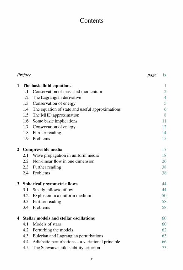
Contents
Preface page ix
1 The basic fluid equations 11.1 Conservation of mass and momentum 21.2 The Lagrangian derivative 41.3 Conservation of energy 51.4 The equation of state and useful approximations 61.5 The MHD approximation 81.6 Some basic implications 111.7 Conservation of energy 121.8 Further reading 141.9 Problems 15
2 Compressible media 172.1 Wave propagation in uniform media 182.2 Non-linear flow in one dimension 262.3 Further reading 382.4 Problems 38
3 Spherically symmetric flows 443.1 Steady inflow/outflow 443.2 Explosion in a uniform medium 503.3 Further reading 583.4 Problems 58
4 Stellar models and stellar oscillations 604.1 Models of stars 604.2 Perturbing the models 624.3 Eulerian and Lagrangian perturbations 634.4 Adiabatic perturbations – a variational principle 664.5 The Schwarzschild stability criterion 73
v
vi Contents
4.6 Further reading 744.7 Problems 75
5 Stellar oscillations – waves in stratified media 785.1 Waves in a plane-parallel atmosphere 795.2 Vertical waves in a polytropic atmosphere 845.3 Further reading 875.4 Problems 87
6 Damping and excitation of stellar oscillations 906.1 A simple set of oscillations 916.2 Damping by conductivity 926.3 The effect of heating and cooling – the ε-mechanism 956.4 The effect of opacity – the κ-mechanism 976.5 Further reading 101
7 Magnetic instability in a static atmosphere 1027.1 Magnetic buoyancy 1027.2 The Parker instability 1067.3 Further reading 1117.4 Problems 111
8 Thermal instabilities 1138.1 Linear perturbations and the Field criterion 1148.2 Heating and cooling fronts 1188.3 Further reading 1208.4 Problems 120
9 Gravitational instability 1239.1 The Jeans instability 1239.2 Isothermal, self-gravitating plane layer 1259.3 Stability of a thin slab 1289.4 Further reading 1309.5 Problems 131
10 Linear shear flows 13410.1 Perturbation of a linear shear flow 13510.2 Squire’s theorem 13610.3 Rayleigh’s inflexion point theorem 13610.4 Fjørtoft’s theorem 138
Contents vii
10.5 Physical interpretation 13910.6 Co-moving phase 14110.7 Stratified shear flow 14210.8 The Richardson criterion 14410.9 Further reading 14510.10 Problems 145
11 Rotating flows 15011.1 Rotating fluid equilibria 15011.2 Making rotating stellar models 15111.3 Meridional circulation 15411.4 Rotation and magnetism 15611.5 Further reading 15711.6 Problems 157
12 Circular shear flow 15812.1 Incompressible shear flow in a rigid cylinder 15812.2 Axisymmetric stability of a compressible rotating flow 16212.3 Circular shear flow with a magnetic field 16712.4 Circular shear flow with self-gravity 17212.5 Further reading 17612.6 Problems 176
13 Modes in rotating stars 17813.1 The non-rotating ‘star’ 17813.2 Uniform rotation 18113.3 Further reading 18713.4 Problems 187
14 Cylindrical shear flow–non-axisymmetric instability 19114.1 Equilibrium configuration 19114.2 The perturbation equations 19314.3 The Papaloizou–Pringle instability 19514.4 Further reading 19714.5 Problems 197
References 199
Index 203

Preface
Almost all of the baryonic Universe is fluid, and the study of how these fluidsmove is central to astrophysics. This book originated in a 24-lecture course entitled‘Astrophysical Fluids’ given by one of us (JEP) in Part III of the MathematicalTripos at the University of Cambridge, comparable in level to a graduate coursein the USA. The course was intended as a preparation for research, and the bookreflects this. Preparing the lecture course and especially its booklist made it plainthat there was a need to bring these ideas together in one place.
The book provides a brief coverage of basic concepts, but does assume somefamiliarity with undergraduate-level fluid dynamics, electromagnetic theory andthermodynamics. Our aim is to give a flavour of the fundamental fluid dynamicalprocesses and concepts which an astrophysical theorist ought to know. To keep thebook to a manageable size, we have had to be selective. In particular, we omit alldiscussion of dissipative fluid processes such as viscosity and magnetic diffusivity.
As well as covering a range of fluid dynamical concepts, we introducesome mathematical ideas and techniques. None of these is particularly deep orabstract, but some of the implementations do require some moderately heavybut straightforward algebra. Thus the reader will benefit from some familiaritywith undergraduate-level mathematical methods, as well as some facility inmathematical manipulation. This takes practice and care, but more than anythingit requires the ability to spot a mistake before proceeding too far.
Ideally, of course, one does not make mistakes, and some lecturers like to givetheir students the misleading impression that this is how research is done. In practice,errors occur all too frequently, and unfortunately some of these make their wayinto the research literature. The best method for finding errors is to understand thephysical processes involved and how these processes are expressed in mathematicalformulae. For this reason, this book emphasizes physical understanding and theextraction of relevant physical ideas from a mass of equations. To achieve this weoften drastically simplify problems and keep only the physical processes of interest.For example, in the chapters on stellar oscillations we eliminate much of the heavyalgebra which appears because real stars are spherical, and instead assume that starsare square (plane-parallel) or at worst (for rotating stars) cylindrical. This lets usget at the underlying physical processes without obscuring them with mathematics.
ix
x Preface
The problems at the ends of the chapters come both from the problem sheetsassociated with the course and from the examination questions set for it. They areintended to illustrate the course material further and also to introduce additionalideas. Thus they are an integral part of the book, and the determined reader willbenefit from working through them.
1
The basic fluid equations
The subject of this book is how the matter of the visible Universe moves. Almostall of this matter is in gaseous form, and each gram contains of order 1024
particles (atoms, ions, protons, electrons, etc.), all moving independently exceptfor interactions such as collisions. At first sight it might seem an impossible taskto describe the evolution of such a complicated system. However, in many caseswe can avoid most of this inherent complexity by approximating the matter as afluid.Afluid is an idealized continuous medium with certain macroscopic propertiessuch as density, pressure and velocity . This concept applies equally to gases andliquids, and we shall take the term fluid to refer to both in this book. The structure ofmatter at the atomic or molecular level is important only in fixing relations betweenmacroscopic fluid properties such as density and pressure, and in specifying otherssuch as viscosity and conductivity.
Describing a medium as a fluid is possible if we can define physical quantitiessuch as density ρ(r, t) or velocity u(r, t) at a particular place with position vectorr at time t. For a meaningful definition of a ‘fluid velocity’ we must averageover a large number of such particles. In other words, fluid dynamical quantitiesare well defined only on a scale l such that l is not only much greater than atypical interparticle distance, but also, more restrictively, much greater than a typicalparticle mean free path, λmfp.† Further, the concept of local fluid quantities is onlyuseful if the scale l on which they are defined is much smaller than the typicalmacroscopic lengthscales L on which fluid properties vary. Thus to use the equationsof fluid dynamics we require L � l � λmfp.
If this condition fails one should, strictly, not apply the fluid dynamical equations,but instead use concepts from plasma physics such as particle distribution func-tions. However, the huge additional complications and large physical uncertainties
† Roughly speaking, the mean free path is the average distance travelled by a typical particle before itstrajectory is significantly deflected by another particle.
1
2 The basic fluid equations
involved here mean that astrophysicists often apply fluid dynamical equations insituations where they are not strictly valid. The mean free path in astrophysical fluidsis typically λmfp�106(T 2/n) cm, where T is the temperature (in K) and n is the num-ber density (in cm−3). In the centre of the Sun we have T � 107 K, n � 1026 cm−3,so λmfp ∼ 10−6 cm. This is far smaller than the solar radius R� = 7×1010 cm, so thefluid approximation is very good. In the solar wind, however, we have T ∼ 105 K,n ∼ 10 cm−3 near the Earth’s orbit, so that λmfp ∼ 1015 cm. This is far greater thanthe Sun–Earth distance, which is 1.5 × 1013 cm. Thus the fluid approximation doesnot apply well here, and the treatment of the interaction of the solar wind with theEarth’s magnetosphere requires plasma physics. As a final example, the diffuse gasin a cluster of galaxies typically has T � 3 × 10⁷ K, n � 10−3 cm−3, and henceλmfp ∼ 1024 cm. This is of the same order as the physical size ∼ 1 Mpc of a richcluster. The fluid approximation is at best marginal for the diffuse regions of thecluster gas, but is nevertheless often used to gain a crude insight into its dynamics,heating and cooling. The dimensionless ratio λmfp/L of mean free path to typicalflow lengthscale is called the Knudsen number Kn; Kn � 1 is a necessary conditionfor the validity of the fluid approximation. The results above show that Kn � 1 inthe interior of the Sun, Kn � 1 in the solar wind, and Kn ∼ 1 in cluster gas.
In this book we assume that the reader already has some familiarity with fluiddynamics, though not necessarily in an astrophysical context. For this reason thefollowing derivation and discussion of the equations of fluid dynamics is brief.It is aimed mainly at establishing notation, as well as stressing those properties offluids relevant to astrophysics which may be less familiar to fluid dynamicists fromother fields.
1.1 Conservation of mass and momentum
The equations of fluid dynamics express conservation laws, and indeed one can usethis basic property advantageously in devising numerical methods to solve them.
1.1.1 Mass conservation
Consider a fixed finite volume V within the fluid, bounded by the surface S. Thenthe mass of fluid contained within the volume is given by∫
Vρ dV . (1.1)
The mass contained in V can change only through a flux of fluid through thesurface S. Thus conservation of mass implies the following:
d
dt
∫V
ρ dV = −∫
Sρu · dS, (1.2)
1.1 Conservation of mass and momentum 3
where dS is the (vector) element of area on the surface S. The volume is fixed, sowe can take the derivative inside the term on the left-hand side (l.h.s.) and applythe divergence theorem to the term on the right-hand side (r.h.s.) to obtain∫
V
{∂ρ
∂t+ div(ρu)
}dV = 0. (1.3)
Since the volume V is arbitrary, we conclude that the integrand must itself vanish,that is
∂ρ
∂t+ div(ρu) = 0, (1.4)
and, equivalently, in suffix notation
∂ρ
∂t+ ∂
∂xj(ρuj) = 0. (1.5)
1.1.2 Momentum conservation
The momentum equation is obtained in exactly the same way by considering therate of change of the total momentum in the volume V , given by
d
dt
∫V
ρ u dV . (1.6)
The additional complication here is that as well as considering the flux ofmomentum across the surface S, we must take account of both the body forceper unit volume fi acting on the fluid and the surface stress given by an appropriatestress tensor Tij. The momentum equation is then given by
∂
∂t(ρui) + ∂
∂xj(ρuiuj) = fi + ∂
∂xj[Tij]. (1.7)
In this book we consider two main contributors to the body force. First we writethe gravitational force as follows:
fi = −ρ∂�
∂xi, (1.8)
where the gravitational potential � is related to the density through Poisson’sequation:
∇2� = 4πGρ, (1.9)
where G is the gravitational constant. Second we take the magnetic force in thefollowing form:
fi = (j ∧ B)i, (1.10)
where j is the current and B is the magnetic field.
4 The basic fluid equations
We shall also briefly consider the electric force,
fi = ρQ Ei, (1.11)
where ρQ is the electric charge density and E is the electric field.We define the stress tensor as follows. Consider an infinitesimal vector surface
element dS within the fluid, where by convention the magnitude of the vector is thearea of the surface element and the direction of the vector is normal to the surfaceelement. Then the surface element is subject to a surface force F given by
Fi = Tij dSj. (1.12)
We note that since both dS and F are vectors, then by the quotient rule Tij is asecond-order tensor.
In this book the main contributor to the stress tensor that we consider is thepressure p in the form
Tij = −pδij, (1.13)
where we make use of the Kronecker delta. In Section 1.5 we shall also write themagnetic force as a stress tensor as follows:
mij = BiBj − 1
2δijBkBk . (1.14)
Although we do not consider viscous effects in this book, we note here thatthe viscous stress terms come from relating the viscous contribution to the stresstensor to the second-order tensor ∂ui/∂xj. This contains information about therelative flow of neighbouring fluid elements and is called the (rate of) strain tensor.Physically this expresses the fact that microscopic (especially thermal) motionswithin the ensemble of gas particles can transport momentum over distances oforder the mean free path.
Finally, using the mass conservation equation, eq. (1.4), to replace the term ∂ρ/∂t,we obtain the momentum equation (or the equation of motion of the fluid) in thefollowing form:
∂ui
∂t+ uj
∂ui
∂xj= − 1
ρ
∂p
∂xi− ∂�
∂xi+ ∂mij
∂xj. (1.15)
1.2 The Lagrangian derivative
We can consider the evolution of a fluid quantity like the density ρ(r, t) in twoways. The partial derivative ∂ρ/∂t used above measures the way ρ changes withtime t at a fixed position r. But it is often more useful to consider the rate of changeof the density of a particular fluid element as it moves with the fluid. This rate iscalled the Lagrangian derivative and is denoted by Dρ/Dt. We need to establishthe relationship between these two concepts.
1.3 Conservation of energy 5
Suppose that a particular fluid element is at position r0 at time t = 0, and at alater time t is at a new position r(r0, t). Then the velocity of the fluid element isgiven by
u = ∂
∂tr(r0, t), (1.16)
where the partial derivative is taken at fixed r0. The Lagrangian derivative of (forexample) the density of that particular fluid element is then simply given by
Dρ
Dt= ∂
∂tρ(r(r0, t), t), (1.17)
with the partial derivative taken at fixed r0. Since t appears in two places on the r.h.s.we may expect two terms in the derivative. Using the chain rule and the definitionof u above we obtain
Dρ
Dt= ∂ρ
∂t+ u · ∇ρ. (1.18)
Thus, more generally the operator denoting the rate of change of a quantityfollowing the fluid motion (the Lagrangian derivative) is given by
D
Dt= ∂
∂t+ u · ∇. (1.19)
1.3 Conservation of energy
We consider the heat content of a unit mass of fluid. In terms of thermodynamicquantities, a small change in the internal heat content of this unit mass is given by
T dS = de + p dV , (1.20)
where T is the temperature, S is the entropy per unit mass, e is the internal energyper unit mass and V is the volume per unit mass. In terms of the density it is evidentthat V = 1/ρ, and thus
TdS = de − pdρ
ρ2. (1.21)
Hence in a fluid flow, the rate of change of the heat content of a particular fluidelement of unit mass is given by
TDS
Dt= De
Dt− p
ρ2
Dρ
Dt. (1.22)
The heat content of a fluid element can change through effects of two types.First, there may be heat flow into or out of the element. We shall refer to this
generically as ‘conduction’. However, in the astrophysical context heat can beconducted both by gas particles (typically electrons, since they move faster thanthe ions) as in standard thermal conduction and also by photons (known as radiative
6 The basic fluid equations
transfer). In both cases, the heat flux h in units of energy per unit area per unittime can often be written in the following form:
h = −λ∇T, (1.23)
which implies physically that the heat flux occurs down the temperature gradientat a rate proportional to some ‘thermal conductivity’ λ. We expect λ to be afunction of thermodynamic variables such as T and ρ. This form of the heat fluxis appropriate provided that the particles carrying the heat have mean free pathsmuch smaller than the typical lengthscale L over which macroscopic fluid quantitieschange. For electrons or molecules this is equivalent to the requirements of the fluidapproximation, whereas for photons it requires in addition that the fluid shouldbe opaque (‘optically thick’) so that there are very large numbers of interactionsbetween photons and the fluid over lengthscales L.
Second, there may be internal generation of heat. This can result from dissipationof kinetic energy by viscosity or dissipation of magnetic energy through resistivity(or electrical conductivity). We do not consider these processes in this book. In theastrophysical context internal energy can be generated by nuclear processes (suchas nuclear energy generation in stars) and by a change in ionization of the fluid. Itcan also be caused by heat exchange with particles which have a low collision crosssection, for example heating by cosmic rays in the interstellar medium and radiativeheating and/or cooling in an optically thin gas. We shall denote the generation ofinternal energy by ε in units of energy per unit volume per unit time.
To convert from the rate of change of a unit mass of fluid (given by eq. (1.22))to the rate of change per unit volume, we multiply by the mass per unit volume, i.e.the density. Thus the heat equation becomes
ρTDS
Dt= −div h + ε. (1.24)
1.4 The equation of state and useful approximations
To complete the set of equations obtained so far we need a relationship of the formp = p(ρ, T ), which is the equation of state for the fluid. In this book we shallassume the simplest form of the relationship, namely the equation of state of aperfect gas,
p = Rµ
ρT , (1.25)
where R is the gas constant and µ is the mean particle mass, assumed to be constant.We also note that
Rµ
= cp − cV , (1.26)
1.4 The equation of state and useful approximations 7
where cp = T (∂S/∂T )p is the specific heat at constant pressure and cV =T (∂S/∂T )V is the specific heat at constant volume. Alternatively this may bewritten as follows:
p = (γ − 1)ρe, (1.27)
where γ = cp/cV is the ratio of specific heats, and we note for a perfect gas that
e = cV T . (1.28)
To understand the physics of a particular fluid dynamical situation it is often notnecessary to include the full thermodynamic complexity of the fluid. In these caseswe can simplify and/or circumvent the heat equation.
1.4.1 Incompressible approximation
The major difference between astrophysical fluids and those encountered inmany terrestrial situations (including those encountered in many courses on fluiddynamics) is that astrophysical ones are highly compressible. However, in situationswhere fluid motions are slow compared with the sound speed, density gradientsare quickly smoothed out and it is a useful approximation to treat the fluid as if itwere incompressible. In physical terms this means that any particular element ofthe fluid does not change its density, which implies that
Dρ
Dt= 0. (1.29)
It is important to realise that this does not imply that the fluid itself has constantdensity, so we may not write ρ = constant, unless the original fluid state hasuniform density.
1.4.2 Adiabatic flow
If the flow occurs fast enough that no fluid element has time to exchange heat withits surroundings, and if energy generation within the fluid is negligible, the heatequation simplifies to
DS
Dt= 0. (1.30)
In other words, each fluid element evolves at constant entropy – it remains on thesame adiabat.
At constant entropy we note that
Dp
Dt=(
∂p
∂ρ
)S
Dρ
Dt, (1.31)
8 The basic fluid equations
and that (∂p
∂ρ
)S
= cp
cV
(∂p
∂ρ
)T
. (1.32)
Since for a perfect gas (∂p
∂ρ
)T
= p
ρ, (1.33)
on using γ = cp/cV we obtain
D
Dtln p = γ
D
Dtln ρ. (1.34)
Thus for adiabatic flow we may assume that
D
Dt( p/ργ ) = 0. (1.35)
We note again that this does not imply that the entropy of the fluid is constanteverywhere. But in this case if the fluid is initially isentropic (has uniform entropy)then it remains so.
1.4.3 Barotropic flow
We can avoid using the heat equation, and therefore simplify the analysis, byassuming that pressure is solely a function of density, i.e. p = p(ρ). This isa useful approximation when the detailed thermal properties of the fluid are notdirectly relevant to the dynamics under consideration. Barotropic flow is moregeneral than isentropic flow, and includes isothermal flow (for which p ∝ ρ) aswell as the polytropic approximation to the equation of state (relevant to fullydegenerate matter),
p = Aρ1+1/n, (1.36)
where A and n are constants and n is called the polytropic index.
1.5 The MHD approximation
Astrophysical fluids are usually highly ionized (and so highly conducting) andpermeated by magnetic fields. Understanding the interaction between the fluid andthe magnetic fields it contains is therefore often important. The usual treatment ofthis interaction uses the magnetohydrodynamics (MHD) approximation. We stressthat this is an approximation and that, in common with the fluid approximation, itis often tempting to use it in contexts where its validity is stretched.
We start by considering a fluid flow with a typical flow lengthscale L and typicalflow timescale T . The usual MHD approximation depends on the assumption thatthe resulting typical flow velocity U is much less than the speed of light, i.e.
1.5 The MHD approximation 9
U ∼ L/T � c. The approximation stems from the use of Ohm’s law appliedlocally in the frame of the fluid. Thus we need to be able to transform betweenthe fields (E, B) in the inertial frame and the fields (E′, B′) in the frame of thefluid, which is moving with velocity u. These are related by the usual Lorentztransformation:
E′ = (1 − γ )
(u · Eu2
)u + γ (E + u ∧ B), (1.37)
and
B′ = (1 − γ )
(u · Bu2
)u + γ
(B − 1
c2u ∧ E
), (1.38)
where
γ =(
1 − u2
c2
)−1/2
. (1.39)
Taking the low-velocity approximation u2 � c2 and neglecting terms of order(u2/c2), these relations become
E′ = E + u ∧ B (1.40)
andB′ = B. (1.41)
The time evolution of the magnetic field is determined from the Maxwellequation,
∂B∂t
= −curl E. (1.42)
By comparing dimensional quantities on each side of the equation we see that toorder of magnitude B/T ∼ E/L, or equivalently E ∼ (L/T )B ∼ UB.
The second relevant Maxwell equation is as follows:
µ−10 curl B = j + ε0
∂E∂t
. (1.43)
The second term on the r.h.s. is the displacement current, which permits thepropagation of electromagnetic waves in vacuum with speed c, where c2 = 1/ε0µ0.However, in the MHD approximation we neglect the displacement current. Thisis because the ratio between the displacement current and the term on the l.h.s. isgiven to order of magnitude as (ε0E/T )/(B/µ0L) ∼ (E/B)(U/c2) ∼ U 2/c2 � 1.Thus in the MHD approximation, electromagnetic waves are excluded and thecurrent is given by
j = µ−10 curl B. (1.44)
Since B′ = B, it follows that the current in the frame of the fluid is given by
j′ = j. (1.45)
10 The basic fluid equations
In the frame of the fluid Ohm’s law becomes j′ = σE′, where σ is the conductivity.In this book we make the additional assumption that the conductivity is infinite,which then implies that E′ = 0, i.e. that
E = −u ∧ B. (1.46)
Substituting this into eq. (1.42) we obtain the induction equation,
∂B∂t
= curl(u ∧ B), (1.47)
which describes the time evolution of the magnetic field in the ideal MHDapproximation.
We also need to consider the electromagnetic force acting on the fluid. TheLorentz force is given by
f = ρQ E + j ∧ B. (1.48)
The charge density ρQ is related to the electric field E through the followingMaxwell equation:
div E = ρQ/ε0. (1.49)
Thus the ratio between the electric and magnetic contributions to the Lorentz forceon the fluid is (using eq. (1.44)) to order of magnitude (ε0E2/L)/(B2/Lµ0) ∼U 2/c2. Further, the current ρQu supplied by the moving charge density is also∼U 2/c2 times the current j. Thus in the MHD approximation we can neglect boththe electric charge and the electric field, and the electromagnetic force on the fluidis (using eq. (1.44)) simply given by
f = µ−10 (curl B ∧ B). (1.50)
We can write this as
fi = ∂mik
∂xk, (1.51)
where
mik = µ−10
(BiBk − 1
2B2δik
), (1.52)
and we have used the final Maxwell equation,
div B = 0. (1.53)
1.5.1 Notation and units
We can now see that in the MHD approximation the electric field does not appear inany of the equations. The magnetic field appears only in the induction equation andin the Lorentz force. The induction equation is already dimensionally consistentand so does not change if different units are used for B. In the Lorentz force the
1.6 Some basic implications 11
magnetic field only enters in the dimensional combination [B2/µ0] and the fieldis measured in tesla. In cgs units the magnetic field is measured in gauss and thiscombination should be replaced by [B2/4π ]. Throughout the rest of this book weshall simplify the analysis and omit the factor of µ−1
0 (or of 1/4π ).
1.6 Some basic implications
Here we note some basic results which will prove useful in later chapters and whichhelp to provide a simple mental picture of some of the results we shall derive.
1.6.1 Bernoulli equation for a non-magnetic barotropic fluid
For a barotropic fluid we have p = p(ρ) and we can define the quantity h = ∫dp/ρ.
Then, in a gravitational potential �, the momentum equation becomes
∂u∂t
+ (u · ∇)u = −∇h − ∇�. (1.54)
Using the vector identity
(u · ∇)u = ∇(
1
2u2)
− curl u, (1.55)
we can rewrite this as
∂u∂t
− u ∧ curl u = −∇(
1
2u2 + h + �
). (1.56)
If the flow is steady, then taking the scalar product with u implies
u · ∇(
1
2u2 + h + �
)= 0, (1.57)
and thus that the quantity (12u2 + h + �) is constant on streamlines.
1.6.2 Advection of vortex lines
Consider a small line element dl(r, t) in the fluid connecting two neighbouring fluidelements at positions r and r + dl. Then as the fluid elements move, so does theline element dl. It is straightforward to show (see Problem 1.9.1) that the evolutionof the line element is governed by the following equation:
D
Dtdl = (dl · ∇)u. (1.58)
We define the vorticity at a point in the fluid as
ω = curl u. (1.59)
12 The basic fluid equations
We can think of the vorticity as describing the local rotation rate of the fluid. Wecan obtain some insight into how the vorticity behaves by comparing the motionof vortex lines with the way that the line element connecting two fluid elementsmoves.
Taking the curl of eq. (1.56) yields
∂ω
∂t= curl(u ∧ ω). (1.60)
We now use the vector identity for any two vectors a and b:
curl(a ∧ b) = (b · ∇)a − (a · ∇)b + a div b − b div a, (1.61)
to obtain∂ω
∂t+ (u · ∇)ω − (ω · ∇)u + ω div u = 0. (1.62)
Here we have used the identity for any vector a that div(curl a) = 0, so thatdiv ω = 0. The mass conservation equation (eq. (1.4)) in the form
Dρ
Dt+ ρdiv u = 0 (1.63)
lets us eliminate div u and hence obtain the time-evolution equation for the vorticityin the following form:
D
Dt
(ω
ρ
)=[(
ω
ρ
)· ∇]
u. (1.64)
By comparing this equation with eq. (1.58) we see that the quantity ω/ρ, variouslyknown as the vortensity or the potential vorticity, is advected with the fluid.
1.6.3 Advection of magnetic field lines
Equation (1.47) describing the time evolution of magnetic field B is exactly similarto eq. (1.60) describing the evolution of the vorticity ω. Thus the same analysis canbe applied to B, and we obtain
D
Dt
(Bρ
)=[(
Bρ
)· ∇]
u. (1.65)
Thus we can also conclude that the quantity B/ρ is advected with the fluid. In otherwords, in the MHD approximation, and in the absence of dissipation, the magneticfield lines are carried along with the fluid flow.
1.7 Conservation of energy
Finally in this chapter we consider the equations describing the conservation ofenergy. The equations are derived directly from those given above, and so in
1.7 Conservation of energy 13
physical terms they contain no new information. However, it is instructive to seethe combined energy equation in conservative form. To do this we take the equationdescribing the evolution of the thermal energy density ρe of the fluid, and add to itterms describing the evolution of the kinetic energy density 1
2ρu2 and the magneticenergy density 1
2B2.
1.7.1 Kinetic energy
The rate of change of kinetic energy density is given by
∂
∂t
(1
2ρuiui
)= 1
2uiui
∂ρ
∂t+ ρui
∂ui
∂t. (1.66)
On the r.h.s. we use the mass conservation equation, eq. (1.4), to replace ∂ρ/∂tand use the momentum equation, eq. (1.15), to replace ∂ui/∂t. Combining variousterms we then obtain
∂
∂t
(1
2ρu2
)= − ∂
∂xi
[(p + 1
2ρu2
)ui
]− p
ρ
Dρ
Dt+ ui
∂mij
∂xj− ρui
∂�
∂xi. (1.67)
1.7.2 Magnetic energy
The rate of change of magnetic energy density is given by
∂
∂t
(1
2B2)
= B · ∂B∂t
. (1.68)
Using the Maxwell equation
∂B∂t
= −curl E (1.69)
and the vector identity
div(E ∧ B) = B · curl E − E · curl B, (1.70)
this becomes∂
∂t
(1
2B2)
= −div(E ∧ B) − E · curl B. (1.71)
We use the ideal MHD approximation E + u ∧ B = 0, the Maxwell equationrelating j and curl B, and the definition of the stess tensor mij to obtain the equationin the following form:
∂
∂t
(1
2B2)
= −div(E ∧ B) − ui∂mij
∂xj. (1.72)
14 The basic fluid equations
1.7.3 The combined energy equation
We can now combine the equations governing the time evolution of kinetic andmagnetic energy densities with the equation governing the time evolution ofthermal energy as follows:
∂
∂t(ρe) = −div(ρeu − λ∇T ) + p
ρ
Dρ
Dt+ ε (1.73)
to obtain a total energy equation in the form
∂g
∂t= −div q + r, (1.74)
where
g = ρ
(e + 1
2u2)
+ 1
2B2, (1.75)
qi =[ρ
(e + 1
2u2)
+ p
]ui − λ
∂T
∂xi+ (E ∧ B)i (1.76)
andr = ε − ρu · ∇�. (1.77)
Here g represents the various energy densities – thermal, kinetic and magnetic.(Recall that in the MHD approximation the electric energy density is negligible.)The vector quantity q in eq. (1.74) represents energy fluxes. In square bracketsin the first term of eq. (1.76), in addition to the thermal and kinetic energies, thereis a term pu, which represents the p dV work being done in compressing the fluid.There is also the conducted heat flux and the flux of electromagnetic energy (thePoynting flux). Finally, the quantity r in eqs. (1.74) and (1.77) represents heatloss/gain by the fluid. The first term ε represents local energy generation, forexample by nuclear burning, and the second term represents gravitational energyreleased by flow in the gravitational potential �, here assumed to be fixed in time.
In the rest of this book we will use these equations to study a large variety ofastrophysical fluid phenomena. We shall try throughout to discuss the simplestpossible examples, embodying the essential physics in each case.
1.8 Further reading
Further discussion of the derivation and validity of the equations of fluid dynamicsare to be found in Batchelor (1967, Chap. 1) and Landau & Lifshitz (1959, Chap. I).Aderivation of the equations of magnetohydrodynamics (MHD) is given in Roberts(1967, Chap. 1), who also provides a clear description of the thermodynamicrelations made use of here. More details of these are to be found in Lifshitz &
1.9 Problems 15
Pitaevskii (1980, Chap. 2). A description of the relationship between MHD andplasma physics is given by Sturrock (1994, Chaps. 11, 12).
1.9 Problems
1.9.1 (a) At time t, neighbouring fluid particlesAand B are at position vectors r and r + dl,respectively. At time t + δt, particle A is at r + δtu(r), where u(r) is the velocityfield of the fluid. Similarly, particle B is at r + dl + δtu(r + dl). Use this to showthat the time evolution of the line element dl which joins A and B is given by
D
Dtdl = (dl · ∇)u. (1.78)
Show that in a barotropic fluid the specific vorticity, i.e. ω/ρ, obeys the sameequation.
This shows that vortex lines are carried bodily along in an inviscid, barotropicfluid.
(b) The circulation C around a closed curve � is defined as follows:
C =∮
�
u · dr. (1.79)
If the curve � moves with the fluid (assumed to be inviscid and barotropic), showthat C is a constant.
This is known as ‘Kelvin’s circulation theorem’.(c) For a conducting barotropic fluid with zero magnetic diffusivity, show that
D
Dt
(Bρ
)=(
Bρ
)· ∇u. (1.80)
This shows that magnetic field lines are carried bodily along in a perfectlyconducting fluid.
1.9.2 A smooth circular cylinder of radius a and height h contains fluid of uniform densityρ, rotating uniformly with angular velocity � about the axis of symmetry. Computethe vorticity ω.
(a) Show that in cylindrical polar coordinates, (R, φ, z), the velocity field given by
u = (0, R�(t), z/h), (1.81)
applied for an appropriate time, describes a stretching of the cylinder to a heightof 2h while keeping the density and the rotation uniform.
For incompressible flow it is found that stretching vortex lines leads to anincrease in their strength. Use the vorticity equation to show that this is not thecase here.
(b) Show that the flow field given by
u = (−R/a, R�(t), 0), (1.82)
16 The basic fluid equations
applied for an appropriate time, describes decreasing the radius of the cylinder toa/2 while keeping the density and the rotation uniform. Use the vorticity equationto show that in this case the vorticity does change.
(c) Show that both these results can be deduced simply from consideration ofconservation of angular momentum. Use an appropriate combination of thetwo flow fields to show that the increase in strength of vortex lines as they arestretched in an incompressible fluid is also just a consequence of the conservationof angular momentum.
1.9.3 A simple model for a filament in the solar atmosphere considers gas supportedby a magnetic structure. The configuration is steady and two-dimensional in the(x, z)-plane, with constant gravity g = (0, 0, −g). The magnetic field is given byB = (Bx(x), 0, Bz(x)), and is such that Bz → ±B0 as x → ±∞. Show that Bx(x) isa constant.
Assuming that the gas is isothermal, with sound speed cs, and that the densityρ(x) is a function of x alone, show that
Bz(x) = B0 tanh
{gB0x
2c2s Bx
}(1.83)
and find ρ(x).Sketch the magnetic field lines in the (x, z)-plane, and indicate where the density
is highest.
2
Compressible media
In Chapter 1 we emphasized that one of the major differences between astrophysicalflows and the typical flows encountered in the terrestrial or laboratory context is thatastrophysical fluids are compressible. This means that pressure information takes afinite time to propagate through the fluid. Because this time is often comparable toflow timescales, this gives compressible flows a fundamentally different character.In such flows the sound speed plays a role similar in some respects to that of thespeed of light in the theory of relativity. In particular, sound travel times expressphysical causality. Pressure changes cannot propagate upstream in a supersonicflow. Subtle differences from the causal structure of relativity arise because, unlikethe speed of light, the sound speed is variable and depends on the local propertiesof the fluid.
It is important to remember that all flows are compressible at some level.While the incompressible approximation is extremely useful in studying mostterrestrial flows, intuition based on it is often a misleading guide in the astrophysicalcontext. Moreover the elaborate mathematical apparatus assembled to studyincompressible flows has limited applicability to astrophysical flows. For example,in incompressible fluids the pressure is formally disconnected from the otherfluid variables, and appears only in the equation of motion, and only through itsgradient (this is a mathematical expression of the assumption that it can adjustinstantaneously at each point). Thus, taking the curl of the equation of motioneliminates the pressure from much of the analysis. This explains the prominentrole played by the vorticity in the study of incompressible flows. By contrast, thevorticity and associated concepts such as velocity potentials and stream functionsare of relatively little use in studying astrophysical flows.
In this chapter we consider various properties that are basic to an understandingof flows in compressible media.
17
18 Compressible media
2.1 Wave propagation in uniform media
We start by considering the simplest mechanisms transmitting information incompressible media. If the media are uniform, and not subject to external forces,then the simplest waves are pressure waves (acoustic or sound waves) and magneticwaves. We consider each in turn.
2.1.1 Small-amplitude sound waves
We consider a fluid at rest (velocity u0 = 0), with uniform density ρ0 and uniformpressure p0. Each fluid element is now perturbed by moving it a small distanceξ(r, t). The density then becomes ρ(r, t). We are interested in the small change indensity, known as the density perturbation. In general, we need to take care at thispoint and distinguish between Eulerian and Lagrangian perturbations. We mentionthis distinction briefly here, and return to it in more detail later on.
The Eulerian density perturbation is the change in density at a particularcoordinate point r. It is given by
ρ′(r, t) = ρ(r, t) − ρ0(r, t). (2.1)
The Lagrangian density perturbation is the change in density for the particularfluid element which was at point r prior to the perturbation. It is given by
δρ(r, t) = ρ(r + ξ , t) − ρ0(r, t). (2.2)
By using a Taylor expansion for ρ(r + ξ , t), we note that to first order in ξ ,
δρ = ρ′ + ξ · ∇ρ0. (2.3)
Thus for the stationary uniform medium we are currently considering the two waysof viewing the perturbation are the same since ∇ρ0 = 0, and thus for the time beingwe may take δρ = ρ′.
For the moment, we consider Eulerian perturbations, and assume p = p0 + p′with p′ � p0, ρ = ρ0 + ρ′ with ρ′ � ρ0 and u = 0 + u′ with u′ assumed smallin some appropriate sense. We then substitute these into the equation of massconservation:
∂ρ
∂t+ u · ∇ρ + ρ div u = 0, (2.4)
and retain only small quantities to first-order. This yields
∂ρ′
∂t+ ρ0 div u′ = 0. (2.5)
Similarly, we substitute into the momentum equation as follows:
∂u∂t
+ (u · ∇)u = − 1
ρ∇p (2.6)
2.1 Wave propagation in uniform media 19
and retain only terms linear in small quantities to obtain
∂u′
∂t= − 1
ρ0∇p′. (2.7)
To solve these equations we need to know the relationship between p′ and ρ′.Small perturbations in pressure and density usually give rise to correspondingsmall perturbations in the temperature T . For acoustic waves it is often reasonableto assume that the perturbations occur sufficiently fast such that there is no time fortemperature perturbations to be affected by thermal conduction of heat. If so, thenthe perturbations are ‘adiabatic’ in the sense that individual fluid elements remainon the same adiabat throughout the variations in pressure and density. This impliesthat the Lagrangian entropy perturbation for each fluid element is zero. For fluidon a particular adiabat we have seen that p ∝ ργ . Thus we conclude that
δp
p0= γ
δρ
ρ0. (2.8)
* However, since for a uniform fluid Lagrangian and Eulerian perturbations arethe same, we conclude that, in this case,
p′ =(
γ p0
ρ0
)ρ′. (2.9)
We can now obtain an equation for the relative density perturbation (ρ′/ρ0).Recalling that ρ0 is constant, we take the time derivative of eq. (2.5), and useeqs. (2.7) and (2.9) to obtain
∂2
∂t2
(ρ′
ρ0
)= c2
s ∇2(
ρ′
ρ0
), (2.10)
where the quantity cs is a constant and is defined as
c2s = γ
p0
ρ0. (2.11)
Equation (2.10) is instantly recognizable as the linear wave equation for thequantity ρ′/ρ0 with wave propagation speed equal to cs.
The sound speed cs is a fundamental quantity characterizing a compressible fluid.It fixes the maximum rate at which information about pressure, density, velocityand temperature changes can pass through the fluid and modify its behaviour. Wenote that it is a local quantity defined at each point of the fluid and can vary withposition and time. In general we can write it as follows:
cs =(
∂p
∂ρ
)1/2
, (2.12)
20 Compressible media
where the derivative is evaluated using the energy equation and equation of staterelating p and ρ. For example, if we consider isothermal rather than adiabaticperturbations (a good approximation in some cases), then p0 ∝ ρ0 and we obtain
c2s = p0
ρ0(2.13)
rather than eq. (2.11). The perfect gas law, eq. (1.25), shows that in both casescs ∝ T 1/2. Thus, in general, hotter gases have higher sound speeds.
2.1.2 Fourier transforms and the dispersion relation
An alternative, and often simpler, way of coming to the same conclusion is touse Fourier transforms. We note that the three eqs. (2.5), (2.7) and (2.9) for thelinearized quantities ρ′, u′ and p′ are linear differential equations with coefficientswhich are constant in both space and time. Thus, if we Fourier transform in bothspace and time, the equations for the transformed quantities will be algebraic.Thus, for example, we may consider
p′(k, ω) =∫ ∞
−∞p′(r, t) exp[−i(ωt + k · r)]dt d3k, (2.14)
and similarly for ρ′ and u′. Equivalently, and more simply, we may note that sincethe Fourier transform of ∂p′/∂t is iωp′, and the Fourier transform of ∇p′ is ikp′,we can achieve the same result by substituting
p′(r, t) −→ p′(k, ω) exp[i(ωt + k · r)], (2.15)
together with the corresponding quantities for u′ and p′. For clarity we now drop thetildes and also take as read the factor exp[i(ωt + k · r)] throughout. The equationsbecome
iωρ′ + ρ0ik · u′ = 0, (2.16)
iωu′ + ikρ0
p′ = 0 (2.17)
and
p′ = c2s ρ
′. (2.18)
Taking the scalar product of eq. (2.17) with k, and using eqs. (2.16) and (2.18) toeliminate p′ and ρ′, we obtain the following equation:
(k · u′)[ω2 − k2c2s ] = 0, (2.19)
where k = |k|. Then, provided that k · u′ �= 0, that is provided that ∇ · u′ �= 0,i.e. the perturbations are compressible, we obtain the following relationship:
ω2 = k2c2s . (2.20)
2.1 Wave propagation in uniform media 21
This relationship between the (angular ) wave frequency ω and the wavenumberk is known as a dispersion relation. Note that the period of the wave is P = 2π/ω,the wavelength of the wave is λ = 2π/k and the wavefronts are perpendicular tothe vector k. The phase velocity of the waves is (ω/k)k, and this is the velocityof the wavefronts. The group velocity vg = ∂ω/∂k. This is the velocity at whichthe waves propagate information, i.e. the ‘news’ of pressure, density, velocitychanges, etc.
For these simple acoustic waves we see that the phase velocity and the groupvelocity are the same and that both have magnitude equal to the sound speed cs.Finally, from eq. (2.17) we see that k ∧ u = 0, i.e. curl u = 0, so the acoustic wavesrepresent irrotational perturbations. We conclude that these waves are longitudinalwaves, with no transverse component.
The dispersion relation gives us essentially all the information about theproperties of the waves. We have found this relation by replacing differentialequations with algebraic ones. This is a much simpler procedure for obtaininga description of the nature of wave-like motions.
Large parts of this book will make extensive use of Fourier analysis anddispersion relations in this way. This is particularly true where we deal with smallperturbations, as occurs in discussions of stellar oscillations and the stability ofvarious flows.
2.1.3 Waves in a magnetic medium
We have seen that information travels through a compressible medium at the localsound speed. If the medium also has a magnetic field there are other ways ofcommunicating physical information through it.
We consider the same unperturbed fluid as before, with uniform density ρ0,uniform pressure p0 and zero velocity u0, and add a uniform magnetic field B0.We consider small perturbations as before (i.e. ρ = ρ0 + ρ′, p = p0 + p′ and smallvelocity u) and now have to add the perturbation to the magnetic field in the formB = B0 + b(r, t), where |b| � |B0|. We then substitute these into the relevantequations, using the equilibrium conditions that ∇ρ0 = 0, ∇p0 = 0, u0 = 0 andcurl B0 = 0. We also assume that the perturbations are adiabatic so that, as before,we may write p′ = c2
s ρ′, where c2
s = γ p0/ρ0 is uniform and constant. Then themass conservation equation,
∂ρ
∂t+ div(ρu) = 0, (2.21)
becomes
∂ρ′
∂t+ ρ0 div u = 0, (2.22)
22 Compressible media
and the momentum equation,
ρ∂u∂t
+ ρ(u · ∇)u = −∇p − B ∧ (∇ ∧ B), (2.23)
becomes
ρ0∂u∂t
= −c2s ∇ρ′ + B0 ∧ (∇ ∧ b), (2.24)
while the induction equation,
∂B∂t
= ∇ ∧ (u ∧ B), (2.25)
becomes
∂b∂t
= ∇ ∧ (u ∧ B0). (2.26)
We note that eq. (2.26) implies that
∂
∂t(div b) = 0. (2.27)
We differentiate eq. (2.24) with respect to time, and use eqs. (2.22) and (2.26)to eliminate ∂ρ′/∂t and ∂b/∂t to obtain a linear equation for the velocityperturbation u:
ρ0∂2u∂t2
= c2s ∇{ρ0 div u} − B0 ∧ {∇ ∧ [∇ ∧ (u ∧ B0)]}. (2.28)
We can simplify this a little by defining a vector quantity VA with dimensions ofvelocity as follows:
VA = B0√ρ0
, (2.29)
which we shall call the vectorial Alfvén velocity . Then the equation becomes
∂2u∂t2
− c2s ∇(div u) + VA ∧ {∇ ∧ [∇ ∧ (u ∧ VA)]} = 0. (2.30)
Since each term contains either two time derivatives or two space derivatives, this isclearly a wave equation of some sort. If the magnetic field is zero (i.e. B0 = VA = 0)then the equation reduces to the equation for simple acoustic waves that we hadbefore. But the term involving the magnetic field, with its four cross products,considerably complicates things.
In this case it is simpler to investigate the properties of these waves by usingFourier transforms, or equivalently by substituting u(r, t) = u(k, ω) exp[i(ωt +k · r)]. We noted before that this is equivalent to making the transformations
2.1 Wave propagation in uniform media 23
∂/∂t → iω and ∇ → ik. With these substitutions, eq. (2.30) becomes
−ω2u + c2s k(k · u) − VA ∧ {k ∧ [k ∧ (u ∧ VA)]} = 0. (2.31)
To simplify this we first expand the vector triple product in the square brackets,namely
[k ∧ (u ∧ VA)] = [(k · VA)u − (k · u)VA], (2.32)
and then similarly expand the two resulting vector triple products VA ∧ {k ∧ u} andVA ∧ {k ∧ VA}. This gives the equation in the following form:
[ω2−(k · VA)2]u−(c2s + V 2
A )(k · u)k + (k · VA)(u · VA)k + (k · VA)(k · u)VA = 0.(2.33)
This equation allows us to find the dispersion relation for these waves. As it islinear in u, we can in principle write it in the following form:
Aijuj = 0, (2.34)
where the coefficients of the matrix A are functions of ω and k. The dispersionrelation is then given by
det A = 0, (2.35)
which provides a functional relationship between ω and k. However, while thisdispersion relation contains all the information we require, it clearly does not do soin a particularly transparent form. The complicated nature of the equation meansthat we should not necessarily expect the wavevector k and the group velocityvg = ∂ω/∂k to be in the same direction. We now consider two special cases,for which in fact the wavevector and the group velocities are parallel, and whichserve to illustrate the general properties of the waves. We leave a more complicatedexample to the Problems at the end of the chapter.
2.1.3.1 Wavefronts parallel to the magnetic field
Here we consider the case in which the wavevector k is perpendicular to theunperturbed magnetic field, i.e. k · B0 = 0, which implies k · VA = 0. In this case,eq. (2.33) simplifies to
ω2u − (c2s + V 2
A )(k · u)k = 0. (2.36)
Note that this equation implies that u is parallel to k, i.e. that the waves arelongitudinal. We take the scalar (dot) product of this equation with k, and removethe factor u · k �= 0, to obtain the dispersion relation:
ω2 = (c2s + V 2
A )k2. (2.37)
24 Compressible media
(a)
(b)
(c)
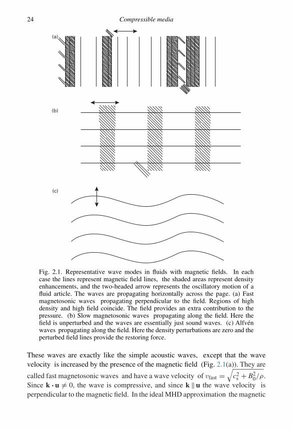
Fig. 2.1. Representative wave modes in fluids with magnetic fields. In eachcase the lines represent magnetic field lines, the shaded areas represent densityenhancements, and the two-headed arrow represents the oscillatory motion of afluid article. The waves are propagating horizontally across the page. (a) Fastmagnetosonic waves propagating perpendicular to the field. Regions of highdensity and high field coincide. The field provides an extra contribution to thepressure. (b) Slow magnetosonic waves propagating along the field. Here thefield is unperturbed and the waves are essentially just sound waves. (c) Alfvénwaves propagating along the field. Here the density perturbations are zero and theperturbed field lines provide the restoring force.
These waves are exactly like the simple acoustic waves, except that the wavevelocity is increased by the presence of the magnetic field (Fig. 2.1(a)). They are
called fast magnetosonic waves and have a wave velocity of vfast =√
c2s + B2
0/ρ.Since k · u �= 0, the wave is compressive, and since k ‖ u the wave velocity isperpendicular to the magnetic field. In the ideal MHD approximation the magnetic
2.1 Wave propagation in uniform media 25
field is carried along with the fluid flow, so the effect of the wave motions is to try tochange the distance between neighbouring magnetic field lines. The magnetic fieldresists this change, and the result is an additional restoring force, which acts exactlyas an added magnetic pressure, and so provides an enhanced wave speed. We notethat this wave exists even in the limit of small gas pressure (or temperature).
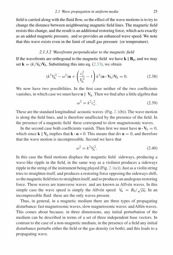
2.1.3.2 Wavefronts perpendicular to the magnetic field
If the wavefronts are orthogonal to the magnetic field we have k ‖ B0, and we mayset k = (k/VA)VA. Substituting this into eq. (2.33), we obtain
(k2V 2A − ω2)u +
(c2
s
V 2A
− 1
)k2(u · VA)VA = 0. (2.38)
We now have two possibilities. In the first case neither of the two coefficientsvanishes, in which case we must have u ‖ VA. Then we find after a little algebra that
ω2 = k2c2s . (2.39)
These are the standard longitudinal acoustic waves (Fig. 2.1(b)). The wave motionis along the field lines, and is therefore unaffected by the presence of the field. Inthe presence of a magnetic field these correspond to slow magnetosonic waves.
In the second case both coefficients vanish. Then first we must have u · VA = 0,which since k ‖ V0 implies that k · u = 0. This means that div u = 0, and thereforethat the wave motion is incompressible. Second we have that
ω2 = k2V 2A . (2.40)
In this case the fluid motions displace the magnetic field sideways, producing awave-like ripple in the field, in the same way as a violinist produces a sidewaysripple in the string of the instrument being played (Fig. 2.1(c)). Just as a violin stringtries to straighten itself, and produces a restoring force opposing the sideways shift,so the magnetic field tries to straighten itself, and so produces an analogous restoringforce. These waves are transverse waves and are known as Alfvén waves. In thissimple case the wave speed is simply the Alfvén speed VA = B0/
√ρ0. In an
incompressible fluid these are the only waves present.Thus, in general, in a magnetic medium there are three types of propagating
disturbance: fast magnetosonic waves, slow magnetosonic waves andAlfén waves.This comes about because, in three dimensions, any initial perturbation of themedium can be described in terms of a set of three independent base vectors. Incontrast to the case of a non-magnetic medium, in the presence of a field any initialdisturbance perturbs either the field or the gas density (or both), and this leads to apropagating wave.
26 Compressible media
We have seen that magnetic wave phenomena introduce the fundamentalpropagation velocity – the Alfvén speed, VA. The Alfvén speed plays a rolein spreading magnetic perturbations similar to that of the sound speed for pressurewaves. One might wonder what happens in the limit of very small density ρ0, whereVA formally becomes infinite. In fact, once ρ0 is small enough that VA formallyexceeds the speed of light c, it is clear that the treatment has become physicallyinconsistent. Then one has to revisit the approximations made in deriving the MHDequations.
2.2 Non-linear flow in one dimension
We have so far considered the properties of small-amplitude perturbations incompressible media. We have seen that such perturbations give rise to waves whichpropagate through the medium at some finite speed. This implies that informationtakes time to travel through the fluid. As we shall see, this finite timescale forthe propagation of information can give rise to problems, for example if the fluidis moving at a velocity greater than the information propagation speed. To clarifysuch questions we consider the simplest case of one-dimensional compressibleflow under pressure forces alone, with no restriction to small perturbations aboutequilibrium.
In one-dimensional flow the fluid quantities are functions of x and t only, and theflow velocity is in the x-direction with magnitude u(x, t). We also assume that theflow is isentropic (the details of the flow are qualitatively similar for other choicesof the relation between p and ρ). The isentropic assumption implies that throughoutthe flow p = Kργ for some constant K and DS/Dt = 0. We take the magnetic fieldto be zero.
With these assumptions, the mass conservation equation becomes
Dρ
Dt+ ρ
∂u
∂x= 0, (2.41)
and the thermal equation (here conservation of entropy) becomes
Dρ
Dt= 1
c2s
Dp
Dt, (2.42)
where the sound speed is given by c2s = γ p/ρ. Eliminating Dρ/Dt from these two
equations, we obtain
1
ρcs
∂p
∂t+ u
ρcs
∂p
∂x+ cs
∂u
∂x= 0. (2.43)
The momentum equation is given by
∂u
∂t+ u
∂u
∂x+ 1
ρ
∂p
∂x= 0. (2.44)
2.2 Non-linear flow in one dimension 27
We now put these two equations together in an illuminating manner. First weadd the two equations and gather terms to yield[
∂u
∂t+ (u + cs)
∂u
∂x
]+ 1
ρcs
[∂p
∂t+ (u + cs)
∂p
∂x
]= 0. (2.45)
Then we subtract the two equations and gather terms to yield[∂u
∂t+ (u − cs)
∂u
∂x
]− 1
ρcs
[∂p
∂t+ (u − cs)
∂p
∂x
]= 0. (2.46)
We note that these two equations are the same except for the change cs ↔ −cs.We can simplify these two equations still further by defining the quantitiesJ+ and J−, known as Riemann invariants:
J+ = u +∫
dp
ρcs(2.47)
and
J− = u −∫
dp
ρcs. (2.48)
Then the two equations become[∂J+∂t
+ (u + cs)∂J+∂x
]= 0 (2.49)
and [∂J−∂t
+ (u − cs)∂J−∂x
]= 0. (2.50)
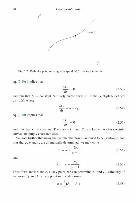
To interpret these equations we first need to consider the meanings of thequantities [· · · ] in square brackets. To do this we consider the (x, t)-plane. Acomplete description of the flow is given by the functions u(x, t) and ρ(x, t) (orequivalently, since it is isentropic, p(x, t)) in this plane. Consider any functionf (x, t) (for example the density ρ(x, t)) in this plane, and consider a curve givenby a monotonic function x = φ(t) in this plane. This curve describes the motion ofsomething which moves at speed dφ/dt along the x-axis (see Fig. 2.2). Then thetime derivative of f (x, t) as seen by this something is given by(
df
dt
)φ
= ∂f
∂t+ dφ
dt
∂f
∂x. (2.51)
We conclude therefore that on the curve C+ in the (x, t)-plane defined by x+(t),where
dx+dt
= u + cs, (2.52)
28 Compressible media
t
x
x = �(t)
Fig. 2.2. Path of a point moving with speed dφ/dt along the x-axis.
eq. (2.49) implies that
dJ+dt
= 0 (2.53)
and thus that J+ = constant. Similarly on the curve C− in the (x, t)-plane definedby x−(t), where
dx−dt
= u − cs, (2.54)
eq. (2.50) implies that
dJ−dt
= 0 (2.55)
and thus that J− = constant. The curves C+ and C− are known as characteristiccurves, or simply characteristics.
We note further that using the fact that the flow is assumed to be isentropic, andthus that p, ρ and cs are all mutually determined, we may write
J+ = u + 2cs
γ − 1(2.56)
and
J− = u − 2cs
γ − 1. (2.57)
Thus if we know u and cs at any point, we can determine J+ and J−. Similarly, ifwe know J+ and J− at any point we can determine
u = 1
2(J+ + J−) (2.58)
2.2 Non-linear flow in one dimension 29
and
cs = γ − 1
4(J+ − J−). (2.59)
The analysis above reveals how information propagates through a compressiblefluid in a remarkably simple way. Sound signals carry the information along thecharacteristics at the local sound speed cs. In subsonic flow, information reachesany given point x = x0 from smaller x < x0 along the C+ characteristic and fromlarger x > x0 along the C− characteristic.
We now discuss two particular sets of implications of this analysis.
2.2.1 Regions of influence
We consider a particular initial-value problem, where we suppose that at time t = 0we have a complete knowledge of the fluid properties, i.e. we know ρ(x, t = 0)
(or, equivalently p(x, t = 0) or cs(x, t = 0)) and u(x, t = 0). We then consider thesolution ρ(x, t) and u(x, t) at later times t > 0. To be specific, consider the functionu(x, t) in the (x, t)-plane (we could also equally well consider the function cs(x, t)).The initial condition at t = 0 is represented by the value of u along the x-axis t = 0.And, of course, the velocity structure at any particular later time t = t0 is given bythe value of u along the line t = t0 parallel to the x-axis in the (x, t)-plane.
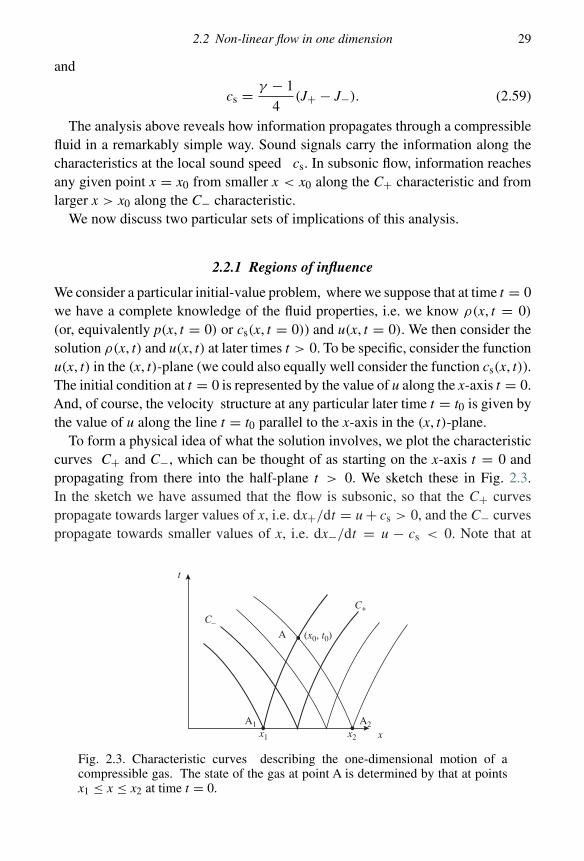
To form a physical idea of what the solution involves, we plot the characteristiccurves C+ and C−, which can be thought of as starting on the x-axis t = 0 andpropagating from there into the half-plane t > 0. We sketch these in Fig. 2.3.In the sketch we have assumed that the flow is subsonic, so that the C+ curvespropagate towards larger values of x, i.e. dx+/dt = u + cs > 0, and the C− curvespropagate towards smaller values of x, i.e. dx−/dt = u − cs < 0. Note that at
t
C–
C+
A1 A2
A
x
(x0, t0)
x1 x2
Fig. 2.3. Characteristic curves describing the one-dimensional motion of acompressible gas. The state of the gas at point A is determined by that at pointsx1 ≤ x ≤ x2 at time t = 0.
30 Compressible media
this stage this can only be a sketch, because in order to draw the curves accurately,we need to know the values of u(x, t) and cs(x, t) at all points in the (x, t)-plane, orin other words we need to have already solved the problem! Now consider the valueof u(x0, t0) at the point A, shown in Fig. 2.3 at position x = x0, t = t0. As shown inFig. 2.3, the characteristic curve C+ which passes through the point (x0, t0) startsat the point A1 with position x1 < x0 at time t = 0. Thus the Riemann invariant J+at A is determined by the initial t = 0 values of u and cs at point A1. That is,
J+(x0, t0) = J+(x1, 0). (2.60)
Similarly, the characteristic curve C− which passes through the point (x0, t0) startsat the point A2 with position x2 > x0 at time t = 0. Thus the Riemann invariantJ− at A is determined by the initial t = 0 values of u and cs at A2. That is,
J−(x0, t0) = J−(x2, 0). (2.61)
Then the values of u and cs at point A are completely determined from thesevalues of J+ and J− by using eqs. (2.58) and (2.59). Thus, for example,
u(x0, t0) = 1
2[J+(x1, 0) + J−(x2, 0)], (2.62)
with a similar equation to determine cs(x0, t0). We note further that, by a similarargument, the values of u and cs at all points on the C+ curve, and therefore theshape of the curve itself in the segment between A1 and A, are determined by theinitial values of u and cs at points on the line segment t = 0, x1 ≤ x ≤ x2. Likewise,the values of u and cs at all points on the C− curve, and therefore the shape of thecurve itself in the segment between A2 and A, are determined by the initial values ofu and cs at points on the same line segment t = 0, x1 ≤ x ≤ x2. Thus the state of thegas at point A depends only on the state of the gas at points A1 and A2, together withthe shapes of the characteristic curves through these points. But the shapes of thecurves depend only on the initial t = 0 state of the gas at points x1 ≤ x ≤ x2. Thusthe state of the gas at point A depends only on the initial state of the gas in a finiteregion. We can see that this comes about because information in a compressiblegas travels only at a finite speed. Thus the state of the gas at point (x0, t0) can onlydepend on the state of those elements of the previous flow which have had time tocommunicate with it. From a physical point of view this is, in retrospect, obvious.This is a basic fact of compressible hydrodynamics, and indeed it is one whichplays a large role in the development of numerical schemes for solving problemsin compressible media.
We see that the system of characteristic curves makes explicit the physicalcausality implicit in the idea of information propagating at a finite speed, herethat of sound. Very similar concepts appear in the theory of relativity, where thefinite speed is of course that of light. Again there is a finite spatial region which is
2.2 Non-linear flow in one dimension 31
able to influence any given event (point in space-time), and this is called the pastlight cone of that point.
2.2.2 Development of shocks
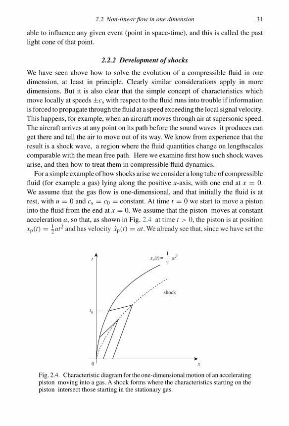
We have seen above how to solve the evolution of a compressible fluid in onedimension, at least in principle. Clearly similar considerations apply in moredimensions. But it is also clear that the simple concept of characteristics whichmove locally at speeds ±cs with respect to the fluid runs into trouble if informationis forced to propagate through the fluid at a speed exceeding the local signal velocity.This happens, for example, when an aircraft moves through air at supersonic speed.The aircraft arrives at any point on its path before the sound waves it produces canget there and tell the air to move out of its way. We know from experience that theresult is a shock wave, a region where the fluid quantities change on lengthscalescomparable with the mean free path. Here we examine first how such shock wavesarise, and then how to treat them in compressible fluid dynamics.
For a simple example of how shocks arise we consider a long tube of compressiblefluid (for example a gas) lying along the positive x-axis, with one end at x = 0.We assume that the gas flow is one-dimensional, and that initially the fluid is atrest, with u = 0 and cs = c0 = constant. At time t = 0 we start to move a pistoninto the fluid from the end at x = 0. We assume that the piston moves at constantacceleration a, so that, as shown in Fig. 2.4 at time t > 0, the piston is at positionxp(t) = 1
2at2 and has velocity xp(t) = at. We already see that, since we have set the
t
t0
0 x
shock
xP(t) = at21
2
Fig. 2.4. Characteristic diagram for the one-dimensional motion of an acceleratingpiston moving into a gas. A shock forms where the characteristics starting on thepiston intersect those starting in the stationary gas.
32 Compressible media
piston velocity to increase linearly with time and therefore eventually to exceed thespeed of sound, we expect the method of solution outlined in the previous sectionto run into trouble.
Again we consider the evolution of the properties of the gas as given by thefunctions u(x, t) and cs(x, t) in the (x, t)-plane. From Fig. 2.4 it is evident that the C−characteristics, which start on the x-axis and move such that dx−/dt = u − cs < 0,fill the whole of the available space. Indeed, until they meet the effects of theadvancing piston, they are straight lines with slope dx/dt = −c0. On all thesecurves, the value of the Riemann invariant J− is the same, and is equal to the value attime t = 0. We conclude that J− is a constant throughout the fluid and is given by
J− = − 2c0
γ − 1. (2.63)
Thus, using the original expression (eq. (2.48)) for J− we see that throughout thefluid cs and u are related by the following expression:
cs = c0 + 1
2(γ − 1)u. (2.64)
Along the C+ curves the quantity J+ = u + 2cs/(γ − 1) is a constant. But since wehave just shown that cs depends only on u throughout the fluid, this implies that alongeach C+ curve both u = constant and cs = constant. Then since dx+/dt = u + cs
we see that the characteristic curves x+(t) are straight lines. A similar argumentapplies to the C− curves.
Now consider the C+ curve x+(t; t0) which originates from the piston at time t =t0, and therefore at position x = 1
2at20 and with velocity u = at0. Using eq. (2.64),
this implies that cs = c0 + 12(γ − 1)at0, and therefore that the characteristic curve
is given by
d
dtx+(t, t0) = c0 + 1
2(γ + 1)at0. (2.65)
Using the initial conditions we can then integrate this to obtain
x+(t, t0) = 1
2at2
0 +{
c0 + 1
2(γ + 1)at0
}(t − t0). (2.66)
We now note that each of the characteristic curves which originate on the pistonis a straight line, and the quantities dx+/dt increase with time t0. Thus as shown inFig. 2.4 in the (x, t)-plane the slopes of the lines decrease with time. This impliesthat they must intersect. This conclusion leads to a contradiction. We have alreadyshown that at any point the fluid properties depend solely on the values J+ and J−of the Riemann invariants, which are constant along the characteristic curves C+and C− passing through that point. But if there are two C+ curves passing througha point, which is what must happen if two such curves intersect, then the fluid
2.2 Non-linear flow in one dimension 33
properties cannot be determined uniquely. But this does not make physical sense. Itis clear that we can set up a physical experiment along the lines described here, andthat the fluid evolution can be determined uniquely. What this implies is not that thefluid cannot make up its mind what to do, but rather that the mathematical methodwe are using to determine its evolution has broken down. As we mentioned at thestart of this section, we know from experience what actually happens. The fluidproperties change over a small region (the size of a few mean free paths) known asa shock. This invalidates the fluid approximation and the mathematical treatmentgiven above in this small region.
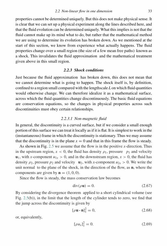
2.2.3 Shock conditions
Just because the fluid approximation has broken down, this does not mean thatwe cannot determine what is going to happen. The shock itself is, by definition,confined to a region small compared with the lengthscale L on which fluid quantitieswould otherwise change. We can therefore idealize it as a mathematical surface,across which the fluid quantities change discontinuously. The basic fluid equationsare conservation equations, so the changes in physical properties across suchdiscontinuities must obey certain relationships.
2.2.3.1 Non-magnetic fluid
In general, the discontinuity is a curved surface, but if we consider a small enoughportion of this surface we can treat it locally as if it is flat. It is simplest to work in the(instantaneous) frame in which the discontinuity is stationary. Thus we may assumethat the discontinuity is in the plane x = 0 and that in this frame the flow is steady.
As shown in Fig. 2.5 we assume that the flow is in the positive x-direction. Thusin the upstream region, x < 0, the fluid has density ρ1, pressure p1 and velocityu1, with x-component u1x > 0, and in the downstream region, x > 0, the fluid hasdensity ρ2, pressure p2 and velocity u2, with x-component u2x > 0. We write theunit normal to the plane of the shock, in the direction of the flow, as n, where thecomponents are given by n = (1, 0, 0).
Since the flow is steady, the mass conservation law becomes
div(ρu) = 0. (2.67)
By considering the divergence theorem applied to a short cylindrical volume (seeFig. 2.5(b)), in the limit that the length of the cylinder tends to zero, we find thatthe jump across the discontinuity is given by
[ρu · n]21 = 0, (2.68)
or, equivalently,
[ρux]21 = 0. (2.69)
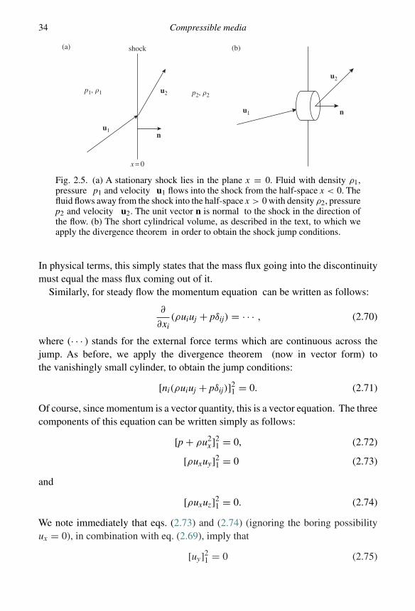
34 Compressible media
p1, �1 p2, �2u2
u2
u1
(a) (b)
u1
n
n
shock
x = 0
Fig. 2.5. (a) A stationary shock lies in the plane x = 0. Fluid with density ρ1,pressure p1 and velocity u1 flows into the shock from the half-space x < 0. Thefluid flows away from the shock into the half-space x > 0 with density ρ2, pressurep2 and velocity u2. The unit vector n is normal to the shock in the direction ofthe flow. (b) The short cylindrical volume, as described in the text, to which weapply the divergence theorem in order to obtain the shock jump conditions.
In physical terms, this simply states that the mass flux going into the discontinuitymust equal the mass flux coming out of it.
Similarly, for steady flow the momentum equation can be written as follows:
∂
∂xi(ρuiuj + pδij) = · · · , (2.70)
where (· · · ) stands for the external force terms which are continuous across thejump. As before, we apply the divergence theorem (now in vector form) tothe vanishingly small cylinder, to obtain the jump conditions:
[ni(ρuiuj + pδij)]21 = 0. (2.71)
Of course, since momentum is a vector quantity, this is a vector equation. The threecomponents of this equation can be written simply as follows:
[p + ρu2x ]2
1 = 0, (2.72)
[ρuxuy]21 = 0 (2.73)
and
[ρuxuz]21 = 0. (2.74)
We note immediately that eqs. (2.73) and (2.74) (ignoring the boring possibilityux = 0), in combination with eq. (2.69), imply that
[uy]21 = 0 (2.75)
2.2 Non-linear flow in one dimension 35
and
[uz]21 = 0. (2.76)
Thus the velocity components parallel to the shock are continuous. We maytherefore, without loss of generality, assume that we can transform to a framein which uy = uz = 0, and replace ux by u.
In a similar manner we may apply the same procedure to the combined energyequation, eq. (1.74). We find that
[q · n]21 = 0, (2.77)
where
q =[ρ
(e + 1
2u2)
+ p
]u. (2.78)
This implies [{ρ
(e + 1
2u2)
+ p
}ux
]2
1= 0. (2.79)
Again, making use of eq. (2.69), this implies[1
2u2 + e + p
ρ
]2
1= 0. (2.80)
The three eqs. (2.69), (2.72) and (2.80) are known as the Rankine–Hugoniotequations. The results of Problem 2.4.3 show that we can turn these into expressionsfor the velocity and density jumps (u2/u1), (ρ2/ρ2) in terms of the (upstream) Machnumber M = u1/cs of the shock.
Physically what happens in a shock is that kinetic energy is turned into heatenergy by dissipation. The result of Problem 2.4.4 shows this explicitly, and we findthat the entropy of the fluid is higher on the downstream side of the shock. Also thesound speed is higher in this post-shock fluid, and comparable with the pre-shockfluid velocity . This is high enough to ensure that the decelerated post-shock fluidnow moves subsonically. By raising the sound speed in this way, the fluid is able tocommunicate the ‘news’ of an obstacle upstream into what would otherwise havebeen a supersonic flow. The high post-shock sound speed occurs because this partof the fluid is hotter. We see that the internal energy e increases across the shock.
Formally it is worth noting that the breakdown of the fluid approximation withinthe shock means that, for example, Bernoulli’s theorem does not hold across it,precisely because the entropy and internal energy increase discontinuously atthe expense of the fluid bulk motion (see eq. (2.80)). As we have seen, dissipationinevitably occurs in shocks, even though it may be negligible (as we have largelyassumed) outside the shock, where the fluid approximation holds.
36 Compressible media
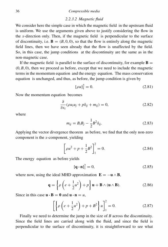
2.2.3.2 Magnetic fluid
We consider here the simple case in which the magnetic field in the upstream fluidis uniform. We use the arguments given above to justify considering the flow inthe x-direction only. Then, if the magnetic field is perpendicular to the surfaceof discontinuity, i.e. B = (B, 0, 0), so that the flow is entirely along the magneticfield lines, then we have seen already that the flow is unaffected by the field.So, in this case, the jump conditions at the discontinuity are the same as in thenon-magnetic case.
If the magnetic field is parallel to the surface of discontinuity, for example B =(0, B, 0), then we proceed as before, except that we need to include the magneticterms in the momentum equation and the energy equation. The mass conservationequation is unchanged, and thus, as before, the jump condition is given by
[ρu]21 = 0. (2.81)
Now the momentum equation becomes
∂
∂xi(ρuiuj + pδij + mij) = 0, (2.82)
where
mij = BiBj − 1
2B2δij. (2.83)
Applying the vector divergence theorem as before, we find that the only non-zerocomponent is the x-component, yielding[
ρu2 + p + 1
2B2]2
1= 0. (2.84)
The energy equation as before yields
[q · n]21 = 0, (2.85)
where now, using the ideal MHD approximation E = −u ∧ B,
q ={ρ
(e + 1
2u2)
+ p
}u + B ∧ (u ∧ B). (2.86)
Since in this case u · B = 0 and u · n = u,[{ρ
(e + 1
2u2)
+ p + B2}
u
]2
1= 0. (2.87)
Finally we need to determine the jump in the size of B across the discontinuity.Since the field lines are carried along with the fluid, and since the field isperpendicular to the surface of discontinuity, it is straightforward to see what
2.2 Non-linear flow in one dimension 37
happens in this case. If, for example, the fluid is denser on the downstream side,then the fluid has been compressed there, and therefore the field lines have beenpushed closer together. Imagine upstream in x < 0 two planes moving with thefluid which are parallel to the discontinuity and which are marked by particular fieldlines. Then when the planes have flowed through the discontinuity downstream inx > 0 the amount of fluid between the two planes is the same. Also the amount ofmagnetic flux between the two plane remains the same. This therefore implies thatthe quantity (B/ρ) remains unchanged. Thus the jump condition for the magneticfield is given by [
Bρ
]2
1= 0. (2.88)
2.2.4 Shock waves in general
We have seen that supersonic motion has a strong tendency to cause shock waves.It is not even necessary for some solid object (e.g. the piston moving into thecylinder that we discussed above) to move itself with supersonic speed for shocksto appear. Let us consider the same initially stationary isentropic gas-filled cylinderand simply move the piston a short distance into it, and then stop the piston entirely,before its own motion becomes supersonic with respect to the cylinder. Physicallyit is clear what happens. Sound waves travel ahead of the piston and tell the gas tomove into the cylinder, raising its pressure and density. But these changes can onlyhappen in the part of the gas close enough to the piston for sound to travel there ina given time. Further away from the piston the gas is unaware of its presence, andremains undisturbed.
One might imagine that once the piston stops moving the result would be asound wave travelling smoothly into this gas. But from eq. (2.11) we can see thatthe sound speed in the gas varies with its density as cs ∝ ρ(γ−1)/2. Since γ > 1,denser gas has a higher sound speed. Hence the compressed gas ahead of the pistonhas a higher sound speed than the undisturbed gas it is trying to push into. Theresult is that the compressed gas becomes still more compressed, further raising thesound speed within it, and further increasing the compression. The density contrastbetween the compressed and undisturbed gas increases until ρ and all other fluidquantities are changing significantly over a mean free path λmfp. This is exactlywhat we mean by a shock. Thus any motion of the piston into the gas ultimatelyleads to the formation of a shock at some distance ahead of it.
This process of density gradients steepening into shocks is already apparentin the characteristic diagram Fig. 2.4. Characteristics starting from the movingcylinder are ‘refracted’ to shallower slopes even before the cylinder itself begins tomove supersonically. These refracted characteristics inevitably intersect the steeper
38 Compressible media
ones in the undisturbed gas at larger x, showing, as expected, that a shock musteventually form.
Of course this does not mean that any isolated disturbance in a compressiblemedium eventually forms a shock wave. Human (and other) life would be verydifferent if this were true! The special feature of the cylinder problem is that thegas is confined and can only move in one direction. In a three-dimensional case,the sound waves from an isolated disturbance spread roughly spherically, and thisgeometrical dilution reverses the tendency for the density to increase ahead of thesound waves. The sound wave spreads to large distances with decreasing amplitudebefore its energy is dissipated in microscopic motions in the gas, i.e. as heat.
Shock waves are extremely common in astrophysics. Gravitational and otherforces can accelerate gas to supersonic speeds, or accelerate objects to move throughgas supersonically. For example, hot stars produce winds which move highlysupersonically into the interstellar medium, producing a system of shock waves,and supernova explosions cause even stronger effects. Similarly, the galaxies ina cluster move supersonically through the cluster gas, heating it via shocks. Anydeceleration or deflection of supersonic gas inevitably leads to shocks, as when gasfalls near radially down magnetic field lines on to a neutron star. The net effect ofshocks is to turn bulk motion into heat, which in turn generally leads to radiation.Hence shocks are very often involved in producing much of the radiation we seefrom high-energy phenomena in the Universe.
2.3 Further reading
The relationship between Lagrangian and Eulerian perturbations is discussedfurther in Chapter 4. The concept of group velocity is described in more detailin Witham (1974, Chap. 11). The derivation of waves in magnetic media givenhere follows that given in Jackson (1998, Chap. 7); an alternative description isgiven by Sturrock (1994, Chap. 14). Non-linear flow of a compressible fluid inone dimension, the concept of characteristics and the development and treatmentof shocks are discussed further in Zel’dovich & Raizer (1967, Chap. I) and inLandau & Lifshitz (1959, Chaps. IX, X). An analogy with traffic flow is describedin Witham (1974, Chap. 3) and in Billingham & King (2000, Chap. 7).
2.4 Problems
2.4.1 Consider waves in a uniform compressible medium with uniform magnetic field Band sound speed cs. In a Cartesian coordinate system, let the wavevector k begiven by
k = (0, 0, k), (2.89)
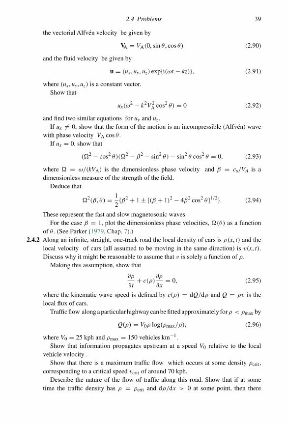
2.4 Problems 39
the vectorial Alfvén velocity be given by
VA = VA(0, sin θ , cos θ) (2.90)
and the fluid velocity be given by
u = (ux, uy, uz) exp{i(ωt − kz)}, (2.91)
where (ux, uy, uz) is a constant vector.Show that
ux(ω2 − k2V 2
A cos2 θ) = 0 (2.92)
and find two similar equations for uy and uz .If ux �= 0, show that the form of the motion is an incompressible (Alfvén) wave
with phase velocity VA cos θ .If ux = 0, show that
(�2 − cos2 θ)(�2 − β2 − sin2 θ) − sin2 θ cos2 θ = 0, (2.93)
where � = ω/(kVA) is the dimensionless phase velocity and β = cs/VA is adimensionless measure of the strength of the field.
Deduce that
�2(β, θ) = 1
2{β2 + 1 ± [(β + 1)2 − 4β2 cos2 θ ]1/2}. (2.94)
These represent the fast and slow magnetosonic waves.For the case β = 1, plot the dimensionless phase velocities, �(θ) as a function
of θ . (See Parker (1979, Chap. 7).)2.4.2 Along an infinite, straight, one-track road the local density of cars is ρ(x, t) and the
local velocity of cars (all assumed to be moving in the same direction) is v(x, t).Discuss why it might be reasonable to assume that v is solely a function of ρ.
Making this assumption, show that
∂ρ
∂t+ c(ρ)
∂ρ
∂x= 0, (2.95)
where the kinematic wave speed is defined by c(ρ) = dQ/dρ and Q = ρv is thelocal flux of cars.
Traffic flow along a particular highway can be fitted approximately forρ < ρmax by
Q(ρ) = V0ρ log(ρmax/ρ), (2.96)
where V0 = 25 kph and ρmax = 150 vehicles km−1.Show that information propagates upstream at a speed V0 relative to the local
vehicle velocity .Show that there is a maximum traffic flow which occurs at some density ρcrit ,
corresponding to a critical speed vcrit of around 70 kph.Describe the nature of the flow of traffic along this road. Show that if at some
time the traffic density has ρ = ρcrit and dρ/dx > 0 at some point, then there
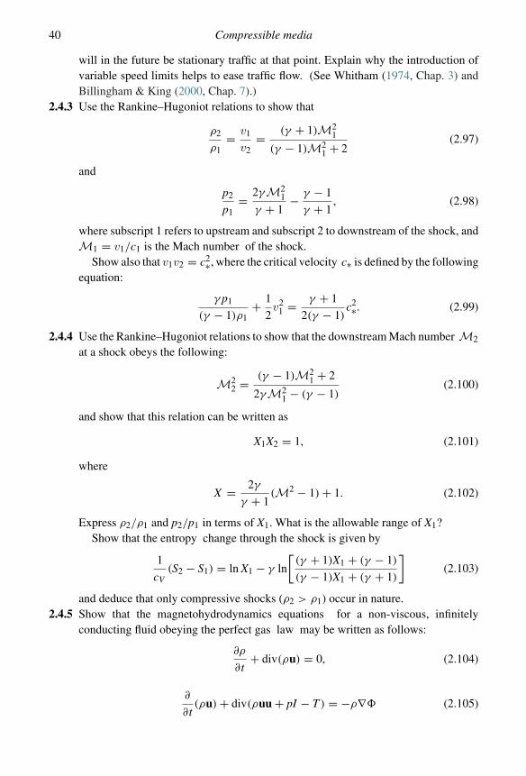
40 Compressible media
will in the future be stationary traffic at that point. Explain why the introduction ofvariable speed limits helps to ease traffic flow. (See Whitham (1974, Chap. 3) andBillingham & King (2000, Chap. 7).)
2.4.3 Use the Rankine–Hugoniot relations to show that
ρ2
ρ1= v1
v2= (γ + 1)M2
1
(γ − 1)M21 + 2
(2.97)
and
p2
p1= 2γM2
1
γ + 1− γ − 1
γ + 1, (2.98)
where subscript 1 refers to upstream and subscript 2 to downstream of the shock, andM1 = v1/c1 is the Mach number of the shock.
Show also that v1v2 = c2∗, where the critical velocity c∗ is defined by the followingequation:
γ p1
(γ − 1)ρ1+ 1
2v2
1 = γ + 1
2(γ − 1)c2∗. (2.99)
2.4.4 Use the Rankine–Hugoniot relations to show that the downstream Mach number M2
at a shock obeys the following:
M22 = (γ − 1)M2
1 + 2
2γM21 − (γ − 1)
(2.100)
and show that this relation can be written as
X1X2 = 1, (2.101)
where
X = 2γ
γ + 1(M2 − 1) + 1. (2.102)
Express ρ2/ρ1 and p2/p1 in terms of X1. What is the allowable range of X1?Show that the entropy change through the shock is given by
1
cV(S2 − S1) = ln X1 − γ ln
[(γ + 1)X1 + (γ − 1)
(γ − 1)X1 + (γ + 1)
](2.103)
and deduce that only compressive shocks (ρ2 > ρ1) occur in nature.2.4.5 Show that the magnetohydrodynamics equations for a non-viscous, infinitely
conducting fluid obeying the perfect gas law may be written as follows:
∂ρ
∂t+ div(ρu) = 0, (2.104)
∂
∂t(ρu) + div(ρuu + pI − T ) = −ρ∇� (2.105)
2.4 Problems 41
and
∂
∂t
(1
2ρu2 + ρe + ρ� + 1
2B2)
+ div
[ρu(
E + p
ρ+ 1
2u2 + �
)+ (B ∧ u) ∧ B)
]= ρ
∂�
∂t, (2.106)
where I is the unit tensor, and the tensor T is given by
T =(
BB − 1
2B2I
). (2.107)
Show that in a steady hydromagnetic shock, in which the magnetic field and theflow velocity are normal to the shock front, the jump conditions across the shockfront are the usual Rankine–Hugoniot conditions. Give a brief physical explanationof why the magnetic field plays no role in this case.
Now consider the jump conditions for a steady hydromagnetic shock in whichthe magnetic field is parallel to the shock front and the flow velocity is normal to it.Show that B1/ρ1 = B2/ρ2, where the subscripts 1 and 2 refer to pre- and post-shockvelocities, respectively.
Show that the jump conditions concerning conservation of mass and momentumimply that
p2 = p1 + ρ1u21
(1 − ρ1
ρ2
)+ B2
1
2
(1 − ρ2
2
ρ21
). (2.108)
Use the jump condition concerning energy conservation to obtain anotherexpression for p2 in terms of the pre-shock variables and the ratio ρ1/ρ2.
Assuming that ρ1 �= ρ2, deduce that x = ρ2/ρ1 is given by the following quadraticequation:
(2 − γ )V 2A1x2 + [(γ − 1)u2
1 + 2c21 + γ V 2
A1]x − (γ + 1)u21 = 0, (2.109)
where c21 = γ p1/ρ1 and V 2
A1 = B21/ρ.
For a shock to exist we require that one of the roots is greater than unity. Showthat this implies the following:
u21 > c2
1 + V 2A1. (2.110)
Give a physical interpretation of this condition. (See Field et al. (1968).)2.4.6 A plane shock wave lies (in the frame of the shock) in the plane x = 0. The flow
velocity is in the x-direction and is of magnitude UL (UR) to the left (right) of theshock, where left (right) corresponds to the half-space x < 0 (x > 0). In the samenotation the densities are ρL (ρR), the pressures are pL (pR) and the energy densitiesare eL (eR). Assuming that the perfect gas law p = (γ − 1)ρe applies on each side
42 Compressible media
of the shock, use the Rankine–Hugoniot relations to show that
ρR
ρL= (γ + 1)M2
L
(γ − 1)M2L + 2
, (2.111)
where ML is the Mach number in x < 0.Deduce that ρR > ρL ⇔ M2
L > 1, and hence that the flow must be supersonic onone side of the shock and subsonic on the other.
Show further that(2
γ + 1
)u2
L + uL(uR − uL) −(
2γ
γ + 1
)pL
ρL= 0, (2.112)
and that (2
γ + 1
)ρLu2
L
pL− pR
pL− γ − 1
γ + 1= 0. (2.113)
Now consider a plane shock lying in the plane x = X (t) < 0 and impinging on astationary solid wall at x = 0. Prior to the passage of the shock the gas is at rest withpressure p0 and density ρ0. As the shock moves towards the wall with steady velocitydX /dt = U+ > 0, the gas behind the shock has velocity us, where 0 < us < U+,pressure ps and density ρs.After the shock has rebounded from the wall it moves withvelocity dX /dt = −U− < 0 into the already once-shocked gas. The gas betweenthe shock and the wall is now stationary and has pressure p1 and density ρ1. Useeq. (2.112) on both the pre- and post-rebound configurations to show that (us + U−)
and (us − U+) both satisfy the same quadratic equation. Deduce that
(us − U+)(us + U−) = −γ ps/ρs. (2.114)
Similarly apply eq. (2.113) to both the pre- and post-rebound configurations andhence, using eq. (2.114), obtain the following relationship:(
2γ
γ + 1
)2
=(
p0
ps+ γ − 1
γ + 1
)(p1
ps+ γ − 1
γ + 1
). (2.115)
In the case of a strong shock (p0 � ps), show that
p1
ps= 3γ − 1
γ − 1. (2.116)
(See Billingham & King (2000).)2.4.7 At time t = 0, an infinite tube contains gas with uniform density and sound speed c0
in the range x > 0 and has a stationary piston at x = 0. For t > 0 the piston movessubsonically with constant velocity −U , where U > 0.
Assume that all the C− characteristics which originate on the line t = 0, x > 0terminate on the piston. Deduce that two C+ characteristics emanate from the positionx = 0, t = 0, one of which (x = c0t) represents the front of a rarefaction wave andthe other of which (x = [c0 − 1
2 (γ + 1)U ]t) represents the back. Show that all otherC+ characteristics are parallel to one or other of these two. Hence sketch all thecharacteristics of the flow in the (x, t)-plane.
2.4 Problems 43
Show that within the rarefaction wave the solution takes the following form:
x = [u + c(u)]t, (2.117)
and deduce that at that point
| u |= 2
γ + 1(c0 − x/t). (2.118)
Use this information to sketch the velocity u(x, t) and the density ρ(x, t) at somelater time t > 0. What happens if U > 2c0/(γ − 1)? (See Landau & Lifschitz (1959,Chap. X) and Zel’dovich & Raizer (1967, Chap. 1.).
3
Spherically symmetric flows
Many astrophysical phenomena are approximately spherically symmetric. Starsare an obvious example, provided that we can neglect the effects of rotation andmagnetic fields. Then the stellar wind is essentially a steady spherical outflow. Butspherical symmetry is often a good description of cases where a fluid with a largelengthscale and little angular momentum is affected by the presence of a smallerobject. An important example of this is gas falling on to a small mass embeddedin it. This may describe a star accreting gas from the interstellar medium, or thecapture of gas by the nucleus of an active galaxy. If conditions far from the centralobject change only slowly we can assume steady inflow or outflow.
3.1 Steady inflow/outflow
We consider a steady, spherically symmetric flow, centred on the origin at whichthere is a point mass, M , with gravitational potential given by
�(r) = −GM
r, (3.1)
where r is the spherical radius. To keep things simple, we neglect thermal processesand assume that the fluid is isentropic. The density ρ(r) and pressure p(r) are justfunctions of radius, r, and the velocity is radial with magnitude u(r), which alsodepends only on the radius r. The mass conservation equation, eq. (1.4), becomes
∂ρ
∂t+ 1
r2
∂
∂r(ρr2u) = 0. (3.2)
Since the situation is steady, we can set ∂ρ/∂t = 0 and then integrate once withrespect to r. The equation then tells us the obvious result that the mass flux, M ,through each spherical shell, radius r, is the same. Thus we can write
4πr2ρu = 4πA, (3.3)
44
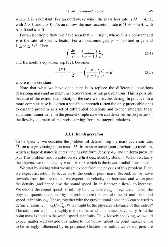
3.1 Steady inflow/outflow 45
where A is a constant. For an outflow, or wind, the mass loss rate is M = 4πA,with A > 0 and u > 0. For an inflow, the mass accretion rate is M = −4πA, withA < 0 and u < 0.
For an isentropic flow we have seen that p = Kργ , where K is a constant andγ is the ratio of specific heats. For a monatomic gas, γ = 5/3 and in general1 ≤ γ ≤ 5/3. Then ∫
dp
ρ=(
γ
γ − 1
)p
ρ, (3.4)
and Bernoulli’s equation, eq. (??), becomes
−GM
r+ 1
2u2 +
(γ
γ − 1
)p
ρ= B, (3.5)
where B is a constant.Note that what we have done here is to replace the differential equations
describing mass and momentum conservation by integral relations. This is possiblebecause of the extreme simplicity of the case we are considering. In practice, in amore complex case it is often a sensible approach (often the only practicable one)to cast the problem as a set of differential equations and to then integrate theseequations numerically. In the present simple case we can describe the properties ofthe flow by geometrical methods, starting from the integral relations.
3.1.1 Bondi accretion
To be specific, we consider the problem of determining the mass accretion rate,M , on to a gravitating point mass, M , from an external (non-gravitating) medium,which at large distance is at rest and has uniform density ρ∞ and uniform pressurep∞. This problem and its solution were first described by Bondi (1952). To clarifythe algebra, we replace u by v = −u > 0, which is the inward radial flow speed.
We start by asking what we might expect from the physics of this problem. First,we expect accretion to occur on to the central point mass. Second, as we moveinwards from infinite radius, we expect the velocity to increase, and we expectthe density (and hence also the sound speed in an isentropic flow) to increase.We denote the sound speed at infinity by c∞, where c2∞ = γ p∞/ρ∞. Then, thephysical quantities defined by the problem are the central mass M and the soundspeed at infinity c∞. These, together with the gravitational constant G can be used todefine a radius rG = GM /c2∞. What might be the physical relevance of this radius?The radius corresponds roughly to the radius at which the escape velocity from thepoint mass is equal to the sound speed at infinity. Thus, loosely speaking, we wouldexpect matter well outside this radius to not ‘know’ about the point mass, i.e. notto be strongly influenced by its presence. Outside this radius we expect pressure
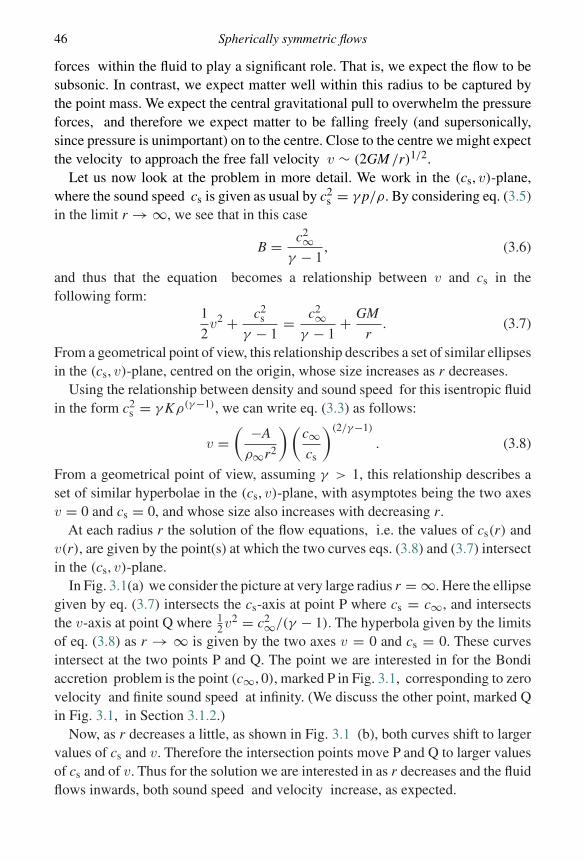
46 Spherically symmetric flows
forces within the fluid to play a significant role. That is, we expect the flow to besubsonic. In contrast, we expect matter well within this radius to be captured bythe point mass. We expect the central gravitational pull to overwhelm the pressureforces, and therefore we expect matter to be falling freely (and supersonically,since pressure is unimportant) on to the centre. Close to the centre we might expectthe velocity to approach the free fall velocity v ∼ (2GM /r)1/2.
Let us now look at the problem in more detail. We work in the (cs, v)-plane,where the sound speed cs is given as usual by c2
s = γ p/ρ. By considering eq. (3.5)in the limit r → ∞, we see that in this case
B = c2∞γ − 1
, (3.6)
and thus that the equation becomes a relationship between v and cs in thefollowing form:
1
2v2 + c2
s
γ − 1= c2∞
γ − 1+ GM
r. (3.7)
From a geometrical point of view, this relationship describes a set of similar ellipsesin the (cs, v)-plane, centred on the origin, whose size increases as r decreases.
Using the relationship between density and sound speed for this isentropic fluidin the form c2
s = γ Kρ(γ−1), we can write eq. (3.3) as follows:
v =( −A
ρ∞r2
)(c∞cs
)(2/γ−1)
. (3.8)
From a geometrical point of view, assuming γ > 1, this relationship describes aset of similar hyperbolae in the (cs, v)-plane, with asymptotes being the two axesv = 0 and cs = 0, and whose size also increases with decreasing r.
At each radius r the solution of the flow equations, i.e. the values of cs(r) andv(r), are given by the point(s) at which the two curves eqs. (3.8) and (3.7) intersectin the (cs, v)-plane.
In Fig. 3.1(a) we consider the picture at very large radius r = ∞. Here the ellipsegiven by eq. (3.7) intersects the cs-axis at point P where cs = c∞, and intersectsthe v-axis at point Q where 1
2v2 = c2∞/(γ − 1). The hyperbola given by the limitsof eq. (3.8) as r → ∞ is given by the two axes v = 0 and cs = 0. These curvesintersect at the two points P and Q. The point we are interested in for the Bondiaccretion problem is the point (c∞, 0), marked P in Fig. 3.1, corresponding to zerovelocity and finite sound speed at infinity. (We discuss the other point, marked Qin Fig. 3.1, in Section 3.1.2.)
Now, as r decreases a little, as shown in Fig. 3.1 (b), both curves shift to largervalues of cs and v. Therefore the intersection points move P and Q to larger valuesof cs and of v. Thus for the solution we are interested in as r decreases and the fluidflows inwards, both sound speed and velocity increase, as expected.
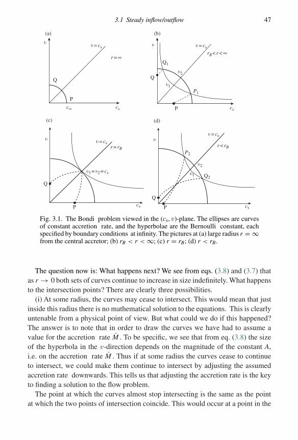
3.1 Steady inflow/outflow 47
Q
P
� = cs�
r = ∞
c∞ cs
�1
�2
P1
Q1
� = cs
rB < r < ∞�
Q
P cs
(c)
�1 = �2 = cs
� = csr = rB
Q
P
�
cs
�2
�1 Q2
P2
� = cs
r < rB
Q
�
P cs
(a)
(d)
(b)
Fig. 3.1. The Bondi problem viewed in the (cs, v)-plane. The ellipses are curvesof constant accretion rate, and the hyperbolae are the Bernoulli constant, eachspecified by boundary conditions at infinity. The pictures at (a) large radius r = ∞from the central accretor; (b) rB < r < ∞; (c) r = rB; (d) r < rB.
The question now is: What happens next? We see from eqs. (3.8) and (3.7) thatas r → 0 both sets of curves continue to increase in size indefinitely. What happensto the intersection points? There are clearly three possibilities.
(i) At some radius, the curves may cease to intersect. This would mean that justinside this radius there is no mathematical solution to the equations. This is clearlyuntenable from a physical point of view. But what could we do if this happened?The answer is to note that in order to draw the curves we have had to assume avalue for the accretion rate M . To be specific, we see that from eq. (3.8) the sizeof the hyperbola in the v-direction depends on the magnitude of the constant A,i.e. on the accretion rate M . Thus if at some radius the curves cease to continueto intersect, we could make them continue to intersect by adjusting the assumedaccretion rate downwards. This tells us that adjusting the accretion rate is the keyto finding a solution to the flow problem.
The point at which the curves almost stop intersecting is the same as the pointat which the two points of intersection coincide. This would occur at a point in the
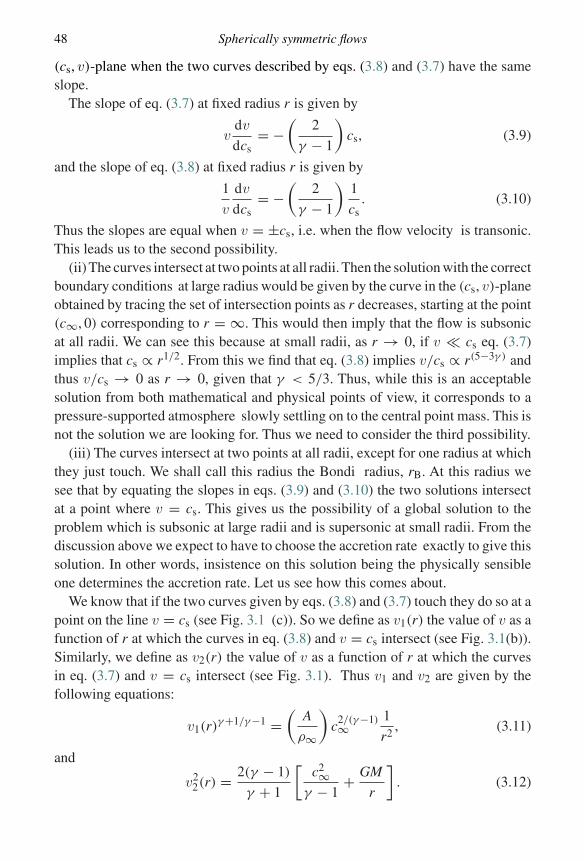
48 Spherically symmetric flows
(cs, v)-plane when the two curves described by eqs. (3.8) and (3.7) have the sameslope.
The slope of eq. (3.7) at fixed radius r is given by
vdv
dcs= −
(2
γ − 1
)cs, (3.9)
and the slope of eq. (3.8) at fixed radius r is given by
1
v
dv
dcs= −
(2
γ − 1
)1
cs. (3.10)
Thus the slopes are equal when v = ±cs, i.e. when the flow velocity is transonic.This leads us to the second possibility.
(ii) The curves intersect at two points at all radii. Then the solution with the correctboundary conditions at large radius would be given by the curve in the (cs, v)-planeobtained by tracing the set of intersection points as r decreases, starting at the point(c∞, 0) corresponding to r = ∞. This would then imply that the flow is subsonicat all radii. We can see this because at small radii, as r → 0, if v � cs eq. (3.7)implies that cs ∝ r1/2. From this we find that eq. (3.8) implies v/cs ∝ r(5−3γ ) andthus v/cs → 0 as r → 0, given that γ < 5/3. Thus, while this is an acceptablesolution from both mathematical and physical points of view, it corresponds to apressure-supported atmosphere slowly settling on to the central point mass. This isnot the solution we are looking for. Thus we need to consider the third possibility.
(iii) The curves intersect at two points at all radii, except for one radius at whichthey just touch. We shall call this radius the Bondi radius, rB. At this radius wesee that by equating the slopes in eqs. (3.9) and (3.10) the two solutions intersectat a point where v = cs. This gives us the possibility of a global solution to theproblem which is subsonic at large radii and is supersonic at small radii. From thediscussion above we expect to have to choose the accretion rate exactly to give thissolution. In other words, insistence on this solution being the physically sensibleone determines the accretion rate. Let us see how this comes about.
We know that if the two curves given by eqs. (3.8) and (3.7) touch they do so at apoint on the line v = cs (see Fig. 3.1 (c)). So we define as v1(r) the value of v as afunction of r at which the curves in eq. (3.8) and v = cs intersect (see Fig. 3.1(b)).Similarly, we define as v2(r) the value of v as a function of r at which the curvesin eq. (3.7) and v = cs intersect (see Fig. 3.1). Thus v1 and v2 are given by thefollowing equations:
v1(r)γ+1/γ−1 =
(A
ρ∞
)c2/(γ−1)∞
1
r2, (3.11)
and
v22(r) = 2(γ − 1)
γ + 1
[c2∞
γ − 1+ GM
r
]. (3.12)
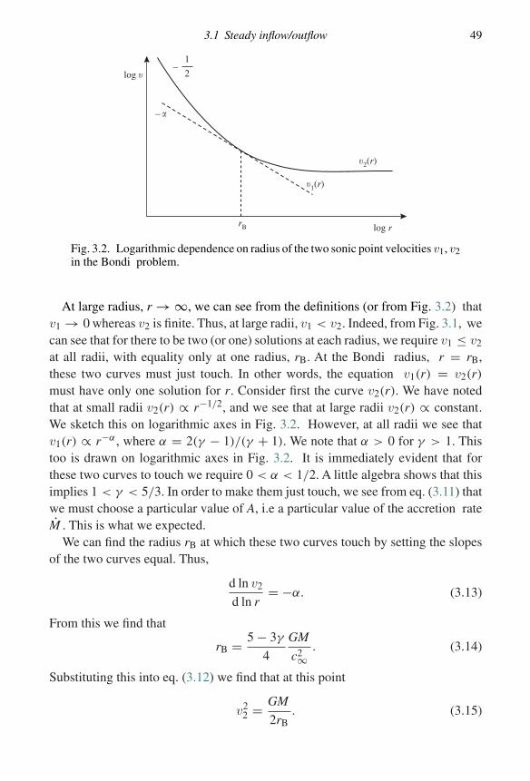
3.1 Steady inflow/outflow 49
log �
log r
– �
–1
2
�2(r)
�1(r)
rB
Fig. 3.2. Logarithmic dependence on radius of the two sonic point velocities v1, v2in the Bondi problem.
At large radius, r → ∞, we can see from the definitions (or from Fig. 3.2) thatv1 → 0 whereas v2 is finite. Thus, at large radii, v1 < v2. Indeed, from Fig. 3.1, wecan see that for there to be two (or one) solutions at each radius, we require v1 ≤ v2
at all radii, with equality only at one radius, rB. At the Bondi radius, r = rB,these two curves must just touch. In other words, the equation v1(r) = v2(r)must have only one solution for r. Consider first the curve v2(r). We have notedthat at small radii v2(r) ∝ r−1/2, and we see that at large radii v2(r) ∝ constant.We sketch this on logarithmic axes in Fig. 3.2. However, at all radii we see thatv1(r) ∝ r−α , where α = 2(γ − 1)/(γ + 1). We note that α > 0 for γ > 1. Thistoo is drawn on logarithmic axes in Fig. 3.2. It is immediately evident that forthese two curves to touch we require 0 < α < 1/2. A little algebra shows that thisimplies 1 < γ < 5/3. In order to make them just touch, we see from eq. (3.11) thatwe must choose a particular value of A, i.e a particular value of the accretion rateM . This is what we expected.
We can find the radius rB at which these two curves touch by setting the slopesof the two curves equal. Thus,
d ln v2
d ln r= −α. (3.13)
From this we find that
rB = 5 − 3γ
4
GM
c2∞. (3.14)
Substituting this into eq. (3.12) we find that at this point
v22 = GM
2rB. (3.15)
50 Spherically symmetric flows
For the curves to touch, we require them to have not only the same slope, butalso the same values of v. Thus at rB we must set v1(rB) = v2(rB). By doing thiswe determine the accretion rate. This is known as the Bondi accretion rate, MB,given by
MB =(
2
5 − 3γ
) γ+12(γ−1) · 4πr2
Bρ∞c∞. (3.16)
We note that this result makes physical sense. We argued earlier that some radiusrG ∼ GM /c2∞ would play an important physical role, and find that this is given bythe Bondi radius rB. To order of magnitude the accretion rate we get is simply thevalue we obtain from a flow through the sphere at r = rB, at speed c∞ and withdensity ρ∞. This is what we would guess from the start. The main result of ouranalysis has been to obtain the constant of proportionality.
From Fig. 3.1 we see that at radii rB the two solutions represented by the pointsP and Q interchange. The accretion solution is represented by point P and becomessupersonic inside rB.
We also note that steady, spherically symmetric accretion of an isentropic fluidonto a point mass (Bondi accretion) can only occur if 1 < γ < 5/3. As γ → 5/3,we see that rB → 0 and M → 0. For values of γ larger than 5/3 it is possibleformally to set up a static atmosphere filling the whole of space, extending all theway from the point mass at r = 0 to infinite radius.
3.1.2 Steady outflow
Essentially all of the above analysis applies also to the situation in which the flowis outwards, with velocity u(r) > 0, and with outwardly directed mass loss rateM . This corresponds to an isentropic stellar wind. The relations given by eqs. (3.8)and (3.7) are the same, except that v(r) is replaced by u(r). All we have to do is tofollow the progress of the other point of intersection of the two curves, i.e. point Qin Fig. 3.1. This point starts at zero velocity at r = 0, and stays subsonic as far asthe radius rB. At that point the flow becomes supersonic, and remains so to largeradius. We can see from Fig. 3.1 (d) that as r → ∞, u2 → 2c2∞ and cs → 0.
3.2 Explosion in a uniform medium
Here we consider the effects of an explosion at a point in a uniform medium. Thefirst studies of this problem concerned explosions of nuclear bombs in the Earth’satmosphere. In astronomy this analysis is used to model the effects of the earlystages of the explosion of a supernova in the interstellar medium.
3.2 Explosion in a uniform medium 51
We model the explosion as the instantaneous input of a fixed amount of energyE at time t = 0 at point r = 0 (in a spherical coordinate system) into a uniformbackground medium of density ρ1. The flow is of course now a time-dependent one,and we therefore expect the velocity to be radially outwards and with magnitudeu(r, t). We expect the input of energy at such a large (formally infinite) rate topush the fluid outwards at such a large velocity (formally infinite initially) that itmoves supersonically. In other words, we expect a shock wave to be generated atthe origin at time t = 0 and to move radially outwards at some velocity Us(t).Initially, the shock will be ‘strong’ in the sense that the pressure p2 behind theshock is much greater than the pressure in the pre-shocked gas, i.e. p2 � p1. Thisis equivalent to assuming that the sound speed in the unshocked gas is much lessthan the shock velocity.
With these assumptions, the only physical quantities relevant to the problem arethe initial density ρ1 and the explosion energy E. This comes from assuming thatthe explosion is essentially at a point, whereas in reality there must be an associatedlengthscale. However, we expect the shock wave to spread so rapidly that its sizeis almost immediately much larger than the original explosion scale. All quantitiesappearing in the solution must therefore be combinations of ρ1, E and the timet, and we can use dimensional analysis to find their dependences, at least up todimensionless multiplicative functions.
In terms of mass M , length L and time T , our two defining quantities havedimensions as follows:
ρ1 ∝ [ML−3] (3.17)
andE ∝ [ML2T−2]. (3.18)
Dividing these two equations, we eliminate M to obtain
ρ1
E∝ T2
L5 . (3.19)
Since the l.h.s. is a constant, we conclude that any radius relevant to the problemmust vary as r ∝ t2/5. From this we can deduce two things. First, the shock radiusrs(t) must move outwards as rs ∝ t2/5. Second, all relevant physical quantitiessuch as velocity u(r, t), pressure p(r, t) and density ρ(r, t) depend on radius andtime only through the combination ξ ∝ r/t2/5.
3.2.1 Shock conditions
To proceed we must discuss how the various physical quantities u, p and ρ varyacross a strong shock. The jump conditions across a stationary shock are theRankine–Hugoniot conditions (eqs. (2.69), (2.72) and (2.80)) derived in Chapter 2.
52 Spherically symmetric flows
In Problem 2.4.3, we deduced expressions for the jump in velocity (u2/u1) andthe jump in density (ρ2/ρ1) in terms of the Mach number of the shock M. Fora strong shock we take the limit M → ∞ and obtain, in the frame in which theshock is stationary,
u2
u1= γ − 1
γ + 1(3.20)
andρ2
ρ1= γ + 1
γ − 1. (3.21)
However, here we shall be working in the inertial frame, in which the shock has avelocity Us(t). In the inertial frame, the fluid is at rest until the shock arrives. Thusin the frame of the shock, the fluid enters the shock with speed u1 = Us. Similarly,in the frame of the shock, the fluid leaves the shock with speed u2, and therefore inthe inertial frame, after the shock has passed, the fluid has velocity u′
2 = Us − u2.We deduce that
u′2 =
(2
γ + 1
)Us. (3.22)
The post-shock density is unchanged by a Galilean transformation, and thereforethe post-shock density is simply ρ′
2 = ρ2. In the limit p2 � p1, the Rankine–Hugoniot relation (eq. (2.72)) which describes momentum conservation yields inthe frame of the shock the following:
p2 = ρ1u21 − ρ2u2
2. (3.23)
After a little algebra, we can use the above relations to show that
p2 = 2
γ + 1ρ1U 2
s . (3.24)
3.2.2 Similarity variables
We have already deduced that the flow inside the shock (r < rs) depends on radiusr and time t only in the combination r/t2/5, so we define a dimensionless variable,
ξ = r( ρ1
Et2
)1/5, (3.25)
called a similarity variable. At fixed time t, the value of ξ is just proportional tothe radius r. Thus, in terms of ξ the shock is at some fixed value, say ξ = ξs. Thenthe shock radius is given by
rs(t) = ξs(E/ρ1)1/5t2/5 (3.26)
and the shock velocity, Us = drs/dt, is given byUs
rs= 2
5t. (3.27)
3.2 Explosion in a uniform medium 53
Obviously we would like to write all the physical quantities u, ρ and p indimensional form multiplied by functions of the dimensionless similarity variableξ . Outside the shock the gas is unaffected by the explosion, and the solutionis simply the initial configuration. So for r > rs we have u = 0, ρ = ρ1 andp = p1 ≈ 0. Thus we need only concern ourselves with the solution inside theshock, at radii 0 < r < rs(t), or equivalently 0 < ξ < ξs. Since physical quantitiesinside the shock depend only on ξ , we may write
ρ(r, t) = ρ2A(ξ), (3.28)
or equivalently
ρ(r, t) =(
γ + 1
γ − 1
)ρ1A(ξ), (3.29)
where A(ξ) is a dimensionless function of ξ . The definition of ρ2 requires A(ξs) = 1.Similarly, since the only combination of our fundamental quantities with the
dimensions of velocity is r/t, we may expect that
u(r, t) = λ0(r/t)V (ξ), (3.30)
where λ0 is some constant and V (ξ) is a dimensionless function of ξ . Usingeq. (3.27) we can rewrite this as follows:
u(r, t) = λ′0(Us/rs)rV (ξ), (3.31)
where λ′0 is some other constant. Motivated by the value for the velocity just inside
the shock, given by eq. (3.22), we choose λ′0 such that
u(r, t) =(
2
γ + 1
)Us
(r
rs
).V (ξ), (3.32)
which implies that at r = rs, where ξ = ξs, we have u = u2 and V (ξs) = 1. Tidyingthis up, we obtain
u(r, t) = 4
5(γ + 1)
(r
t
)V (ξ). (3.33)
In a similar fashion, since pressure has dimensions of density times velocitysquared we can write
p(r, t) = C0(r/t)2ρ1B(ξ), (3.34)
where C0 is some constant and B(ξ) is a dimensionless function of ξ . As before,we try to make things simple by choosing the constant C0 such that B(ξs) = 1. Wecan do this by writing
p(r, t) = p2(r/rs)2B(ξ), (3.35)
as then p = p2 when r = rs. Then, using the expressions derived above for p2 andfor rs, we obtain
p(r, t) = 8
25(γ + 1)ρ1
(r
t
)2B(ξ). (3.36)
54 Spherically symmetric flows
We have now achieved our aim of writing u, ρ and p in dimensional terms multipliedby the dimensionless functions A(ξ), V (ξ) and B(ξ), respectively. We can nowdetermine these three functions, and thus the detailed form of the solution, byinserting these expressions into the conservation equations.
3.2.3 The similarity (Taylor–Sedov) equations
In spherical symmetry the mass conservation equation is given by
∂ρ
∂t= 1
r2
∂
∂r(ρr2u). (3.37)
Similarly the momentum conservation equation is given by
∂u
∂t+ u
∂u
∂r= − 1
ρ
∂p
∂r. (3.38)
For the energy conservation equation we assume that the shocked fluid does notcool, so that each fluid element conserves its entropy, i.e. DS/Dt = 0. Then wehave
∂
∂t
[ρ
(e + 1
2u2)]
+ 1
r2
∂
∂r
[r2ρu
(e + p
ρ+ 1
2u2)]
= 0, (3.39)
and we assume a perfect gas so that e = p/(γ − 1)ρ.When making the substitution we use the definition of ξ (eq. (3.25)), and hence
the derivative of ξ with respect to t at fixed r is given by
∂ξ
∂t
∣∣∣∣r= −2ξ
5t, (3.40)
and the derivative of ξ with respect to r at fixed t is given by
∂ξ
∂r
∣∣∣∣t= ξ
r. (3.41)
Thus, in the conservation equations,we use the following relationships:
∂
∂r
∣∣∣∣t= ξ
r
∂
∂ξ
∣∣∣∣t, (3.42)
and, using the similarity assumption that (∂/∂t)ξ = 0,
∂
∂t
∣∣∣∣r= −2ξ
5t
∂
∂ξ
∣∣∣∣t. (3.43)
We need to take a little care when making these substitutions. For this reason, wederive one equation in some detail and leave the other two to the reader. We rewritethe conservation equationin the following form:
∂ρ
∂t+ ∂
∂r(ρu) + 2ρu
r= 0. (3.44)
3.2 Explosion in a uniform medium 55
Substituting for ρ using eq. (3.29) and using eq. (3.40), the first term on the l.h.s.is simply given by
∂ρ
∂t=(
γ + 1
γ − 1
)ρ1
(−2ξ
5t
dA
dξ
). (3.45)
Similarly, using eq. (3.33) also, the third term on the l.h.s. of eq. (3.44) is given by
2ρu
r= 8
5(γ − 1)ρ1
AV
t. (3.46)
A little more care is required when considering the second term on the l.h.s.Substituting for ρ using eq. (3.29) and for u using eq. (3.33), and also using eq. (3.42)we obtain
∂
∂r(ρu) = ξ
r
∂
∂ξ
∣∣∣∣t
{γ + 1
γ − 1ρ1A
4
5(γ + 1)
(r
t
)V
}. (3.47)
The catch here is that we have to take the derivative of the contents of the curlybracket with respect to ξ at fixed t, but the bracket contains both t and r. Beforetaking the derivative, we must therefore replace r by ξ and t using eq. (3.25). Whenwe do this, the second term on the l.h.s. of eq. (3.44) becomes
∂
∂r(ρu) = 4ρ1
5(γ − 1).1
t
d
dξ(ξAV ). (3.48)
We can now gather the three terms together. We note that they each have a factorof 1/t, which we can cancel (if this did not happen it would either be a sign that wehave made an algebraic mistake, or be a sign that the assumed similarity variabledid not work in this case). We obtain finally the mass conservation equation insimilarity form:
−ξdA
dξ+ 2
γ + 1
(3AV + ξ
d
dξ(AV )
)= 0. (3.49)
Similarly, though at greater length, we can obtain the momentum conservationequation in similarity form:
−V − 2
5ξ
dV
dξ+ 4
5(γ + 1)
(V 2 + V ξ
dV
dξ
)= −2
5
γ − 1
γ + 1
1
A
(2B + ξ
dB
dξ
), (3.50)
and, at even greater length, we can obtain the energy equation in similarity form:
− 2(B + AV 2) − 2
5ξ
d
dξ(B + AV 2)
+ 4
5(γ + 1)
(5V (γ B + AV 2) + ξ
d
dξ[V (γ B + AV 2)]
)= 0. (3.51)
These three equations, eqs. (3.49), (3.50) and (3.51), are called the Taylor–Sedovequations.
56 Spherically symmetric flows
3.2.4 Solving the Taylor–Sedov equations
The Taylor–Sedov equations are three, non-linear, first-order, ordinary differentialequations for A, B and V as functions of ξ . We therefore require three boundaryconditions to define a solution. In one sense we have the boundary conditionsalready, since our initial definitions were set up so that at the shock, i.e. at ξ = ξs,we have A(ξs) = B(ξs) = V (ξs) = 1. Thus, if, for example, we turned to acomputer to integrate these equations numerically, starting from ξ = ξs and workingour way inwards, the problem looks as good as solved. But there is a snag. Westill do not know the value of ξs – that is, we do not know where to start ournumerical integration! In some sense, ξs is an eigenvalue of the problem, and weshall have to find some means of determining its value at the same time as wesolve the differential equations. This problem was solved numerically by Taylor(1959a,1959b) and analytically by Sedov (1959). We start by considering the energyequation:
∂
∂t
[ρ
(e + 1
2u2)]
+ 1
r2
∂
∂r
[r2ρu
(e + p
ρ+ 1
2u2)]
= 0, (3.52)
and we integrate both sides of this equation over all space, namely∫∞
0 4πr2 dr,using the perfect gas equation of state e = p/(γ − 1)ρ. The second term makeszero contribution because ru = 0 at both r = 0 and r = ∞. The perfect gas lawe = p/(γ − 1)ρ then requires
d
dt
∫ ∞
0
(p
γ − 1+ 1
2ρu2
)4πr2 dr = 0. (3.53)
The velocity is zero outside the shock, so we can split this integral into two partsas follows:
d
dt
∫ rs(t)
0
(p
γ − 1+ 1
2ρu2
)4πr2 dr + d
dt
∫ ∞
rs(t)
p1
γ − 14πr2 dr = 0. (3.54)
We can neglect the second integral on the l.h.s. since we have assumed throughoutthat p1 � p2. The equation then states physically that the total energy within theshocked fluid is a constant, and this constant is of course just the input energy E.Thus, ∫ rs(t)
0
(p
γ − 1+ 1
2ρu2
)4πr2 dr = E. (3.55)
We can now translate this expression into our similarity variables, which yields
32π
25(γ 2 − 1)
∫ ξs
0[B(ξ) + A(ξ)V 2(ξ)]ξ4 dξ = 1. (3.56)
In passing, we note that the total thermal energy Eth,
Eth = 32πE
25(γ 2 − 1)
∫ ξs
0[B(ξ)]ξ4 dξ , (3.57)
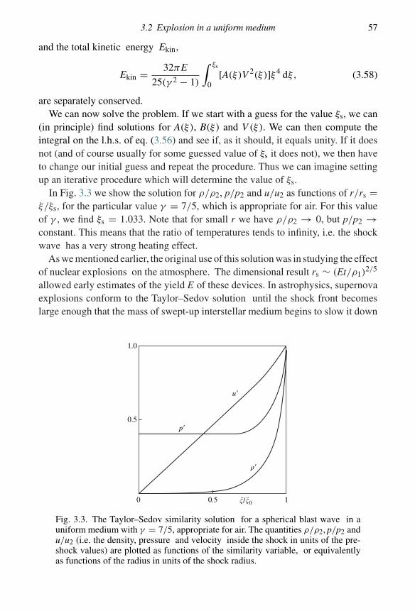
3.2 Explosion in a uniform medium 57
and the total kinetic energy Ekin,
Ekin = 32πE
25(γ 2 − 1)
∫ ξs
0[A(ξ)V 2(ξ)]ξ4 dξ , (3.58)
are separately conserved.We can now solve the problem. If we start with a guess for the value ξs, we can
(in principle) find solutions for A(ξ), B(ξ) and V (ξ). We can then compute theintegral on the l.h.s. of eq. (3.56) and see if, as it should, it equals unity. If it doesnot (and of course usually for some guessed value of ξs it does not), we then haveto change our initial guess and repeat the procedure. Thus we can imagine settingup an iterative procedure which will determine the value of ξs.
In Fig. 3.3 we show the solution for ρ/ρ2, p/p2 and u/u2 as functions of r/rs =ξ/ξs, for the particular value γ = 7/5, which is appropriate for air. For this valueof γ , we find ξs = 1.033. Note that for small r we have ρ/ρ2 → 0, but p/p2 →constant. This means that the ratio of temperatures tends to infinity, i.e. the shockwave has a very strong heating effect.
As we mentioned earlier, the original use of this solution was in studying the effectof nuclear explosions on the atmosphere. The dimensional result rs ∼ (Et/ρ1)
2/5
allowed early estimates of the yield E of these devices. In astrophysics, supernovaexplosions conform to the Taylor–Sedov solution until the shock front becomeslarge enough that the mass of swept-up interstellar medium begins to slow it down
1.0
0.5
0 0.5 1�/�0
��
p�
u�
Fig. 3.3. The Taylor–Sedov similarity solution for a spherical blast wave in auniform medium with γ = 7/5, appropriate for air. The quantities ρ/ρ2, p/p2 andu/u2 (i.e. the density, pressure and velocity inside the shock in units of the pre-shock values) are plotted as functions of the similarity variable, or equivalentlyas functions of the radius in units of the shock radius.
58 Spherically symmetric flows
(the ‘snowplough’phase). More generally, the idea of a similarity solution is usefulin situations where there is a globally conserved quantity (see Sedov (1959) andZel’dovich & Raizer (1967)).
3.3 Further reading
The solution to the problem of steady accretion from a uniform medium waspresented by Bondi (1952). The geometric solution given here is similar to thatgiven in Zel’dovich & Novikov (1971, Chap. 13). Discussion of the similaritysolution for a point explosion in a uniform medium is given in Landau & Lifshitz(1959, Chap. X) and in Shu (1992, Chap. 17). Further information about the use ofsimilarity solutions in solving fluid dynamical problems is to be found in Zel’dovich& Raizer (1967, Chap. XII).
3.4 Problems
3.4.1 In a model of a rocket, a polytropic gas with adiabatic index γ = 2 flows steadilyand adiabatically with velocity v(x) along a smooth nozzle which has slowly varyingcross-sectional area S(x), where x measures the distance along the nozzle. At x = 0,S is very large so that the flow is very subsonic with sound speed c0. Show that thevelocity v(x) and the sound speed c(x) of the gas are related as follows:
1
2v2 + c2 = c2
0, (3.59)
and sketch this relationship in the (v, c)-plane.As x increases, S(x) decreases monotonically to a minimum value Smin at x = xmin
and then increases to a very large value thereafter. The fluid velocity increasesmonotonically. Use mass conservation to plot another relationship in the (v, c)-planefor various values of S(x), taking care to mark the curve corresponding to the valueSmin.
Show that at xmin v = c0√
2/3, and show that the fluid is eventually acceleratedto a velocity of v = c0
√2.
Sketch the pressure profile p(x) and explain how this process might be relevantto astrophysical jets.
(See Blandford & Rees (1974) and Königl (1982).)3.4.2 A fluid flow with radial velocity u(r) and density ρ(r) represents the steady,
spherically symmetric (Bondi) accretion of an isentropic fluid from a surroundingmedium of uniform density ρ∞ onto a gravitating point mass M centred at the origin(r = 0). Show that u(r) and the adiabatic sound speed cs(r) obey the followingequation:
1
u
du
dr= 1
r· GM /r − 2c2
s
c2s − u2
, (3.60)
and find the corresponding equation for dcs/dr.
3.4 Problems 59
Show that at the radius r at which the flow is trans-sonic, the velocity is given byu2 = GM /2r.
Verify that at large radii the equations permit a solution of the form u → 0,ρ → ρ∞ as r → ∞.
Verify that at small radii the equations permit a solution of the form u2 ∼ 2GM /rand u2 � c2
s as r → 0, provided that the ratio of specific heats, γ , is such thatγ < γcrit , where the value of γcrit is to be determined.
A strongly magnetized star, radius R∗, has a dipole field of the form B = ∇ψ ,where, using cylindrical polar coordinates (R, φ, z), we have ψ ∝ z/(R2 + z2)3/2.Bondi-like accretion is taking place in an axisymmetric fashion along the magneticfield lines onto a small circle of radius a (� R∗) at the magnetic pole. Show thatthe cross-sectional area of the flow varies with radius approximately according toA = πa2(r/R∗)3 for A � R2∗.
If the magnetic field is so strong that it remains exactly dipolar, show that it exertsno force on the fluid.
In this case show that the corresponding value of γcrit that allows supersonic flowonto the star is γcrit = 7/5. (See Pringle & Rees (1972).)
4
Stellar models and stellar oscillations
In the next few chapters we consider what happens if we perturb a stationary fluidconfiguration. The unperturbed configuration we have in mind is a body of fluidat rest in a stationary gravitational potential well. This potential might result fromthe self-gravity of the fluid itself, as for a star, or it might be produced by someexternal agency. An example of the latter case is the potential well produced by thedark matter component of a cluster of galaxies. The intracluster medium sits in thispotential, without significantly contributing to it.
Studying perturbations in this way is important for a number of reasons. Wecan often use a linear analysis, and thus make things mathematically tractable.Working out when perturbations grow or not often provides us with a good ideaof how a system will react, even to finite (non-infinitesimal) perturbations. Inparticular, we may be able to decide if the system is likely to react with drasticchanges (instability), or settle down again to a state rather like its original one(stability). A system’s reaction to perturbations also tells us a lot about its structure.Just as geophysicists learn about the Earth’s interior by studying how it reactsto perturbations such as earthquakes, astronomers can use a similar technique(asteroseismology) to study the interior of stars.
4.1 Models of stars
To be specific we shall mainly consider perturbations to models of stars, althoughthe results we find are generally applicable. We first consider briefly what is involvedin making a stellar model. We assume that the star is spherically symmetric and isin hydrostatic equilibrium. This gives us our first two equations.
The star requires a pressure gradient to balance the force of gravity. Thus wemust have
− 1
ρ
dp
dr= d�
dr, (4.1)
60
4.1 Models of stars 61
where, because the star is self-gravitating, the gravitational potential is related tothe stellar density by Poisson’s equation:
1
r2
d
dr
(r2 d�
dr
)= 4πGρ. (4.2)
These two equations can be written as two first-order differential equations bydefining m(r) as the mass within a sphere of radius r, i.e.
m(r) =∫ r
04πr2ρ dr, (4.3)
or, in differential form,
dm
dr= 4πr2ρ. (4.4)
Then the equation of hydrostatic equilibrium becomes
dp
dr= −Gmρ
r2. (4.5)
If the pressure, p, is known as a function of density, ρ, then these two equationsare sufficient to determine the structure of the star. Examples of this case are whitedwarfs and neutron stars, whose matter is completely degenerate. Otherwise wehave to consider the thermal structure of the star, and we need two more equations.First we need energy conservation. If Lr is the outward energy flux throughthe shell at radius r, then in a steady state this energy flux must equal the totalenergy production rate within the sphere of radius r. For most stars the main energyproduction is through nuclear processes, and we may write
Lr =∫ r
04πr2ρεnuc dr, (4.6)
where, in standard notation, εnuc is the energy generation rate per unit mass throughnuclear reactions. In differential form this equation becomes
dLr
dr= 4πr2ρεnuc. (4.7)
Next, we need to describe how the energy produced in the stellar interior makesits way to the surface. Typically we might expect the energy flux per unit area,i.e. Lr/4πr2, to be proportional to the temperature gradient, dT/dr. Often thephysical mechanism for transporting heat is conduction of heat by photons(radiative transfer), which requires
dT
dr= − 3κρ
4acT 3
Lr
4πr2. (4.8)
Here κ is the opacity, which describes the interaction of stellar matter and photonsat the microscopic level, a is the radiation constant and c is the speed of light. This
62 Stellar models and stellar oscillations
equation shows that the net result of the interaction between the stellar radiationfield and matter, consisting of huge numbers of absorptions and re-emissions withinextremely short distances, is a drift of radiant energy down the local temperaturegradient, i.e. radially outwards.
To close the system of equations we require some understanding of the physicalprocesses determining pressure p, opacity κ and energy generation rate εnuc
as functions of local density ρ and temperature T . Under most non-degenerateconditions p is given as a function of ρ and T by the perfect gas law, and theopacity and nuclear energy generation rates are also known as functions ofρ and T . Then the set of four structure equations, which consist of four first-orderdifferential equations for m, p, T and Lr , is well defined, and all we need are someboundary conditions. For a radiative star (i.e. one transporting energy by radiativetransfer as assumed above, rather than by other processes such as convection)these are simple. At the centre, r = 0, we require (by definition) m = Lr = 0,while at the stellar surface, r = R, we require p = 0 and, to a good approximation,T = 0. The latter boundary condition neglects the effect of the star’s atmosphere(the thin outer layer where photons can escape freely into space) on its detailedemission properties. However, this is usually unimportant, since the temperaturehere is far lower than in the stellar interior, and the true temperature profile isextremely close to that given by assuming T = 0 at r = R, except very close to thesurface.
4.2 Perturbing the models
We give here the equations of stellar structure (eqs. (4.4), (4.5), (4.7) and (4.8))for a radiative star in order to illustrate the kind of physical considerations whichgo into making models of stars. There are many excellent books on the intricaciesof making models of stars, and on following the evolution of the models as thestars use up their nuclear fuel. We do not deal with this here. Instead, we ask: Ifwe succeed in making a model of a star, is it stable? If we perturb it a little, whatdoes it do? If the star is stable, we might expect it to oscillate, and perhaps for itsoscillations to be damped. But if it is unstable, then what?
The theory of stellar oscillations is sufficiently complicated that one couldfill a large book on that subject alone. Indeed, several authors already have. Ingeneral, computations detailed enough to compare with observation require oneto retain all the complexity of the original stellar structure equations. This makesnumerical solution unavoidable. In this book, however, we aim to explain the ideasand motivation behind various areas of astrophysical fluid dynamics, rather than topresent the fine details, so we shall try to keep things simple. This means ditchingsome physical reality and hence the ability to compare results with observations
4.3 Eulerian and Lagrangian perturbations 63
in detail. However, we always keep enough of the relevant physics that we canestablish basic physical concepts and principles.
One of the complications of the detailed theory is that stars are spherical, andspherical geometry introduces algebraic complexity. To keep things simple, andthus not obscure the physics with heavy and unilluminating algebra, we consideronly ‘square’ or ‘flat’ stars, which we can treat in Cartesian geometry. Lateron when we consider rotating stars, we shall have to consider cylinders. Clearlythis procedure is not realistic in detail, but it does not do too much violence tothe physics. Aside from losing some factors of π , the main effect we neglect isthat of geometrical spreading in lowering density and compression in raising it.This can be important in some contexts. For example, geometrical spreading is thereason that isolated pressure perturbations do not always lead to shock waves inthree dimensions, whereas this formally always happens in one space dimension,as we saw in Chapter 2. However, the small perturbations we consider generallydo not produce large enough changes in radius for such effects to appear in stellaroscillations.
A further complication occurs if we try to perturb everything simultaneously.Of course this is what happens in reality, but if we attempt this mathematically itis hard to keep track of what causes what. Thus we shall proceed by only allowingsome parts of the physical system to vary at a time, and then only when we wantto understand the results of such a perturbation. Thus we shall ignore the effects ofperturbing the energy equation, except when we wish to look specifically at thestabilizing or destabilizing effects of doing so. Similarly, we ignore perturbations tothe self-gravity of the star (i.e. we shall assume that the gravitational potential isfixed) except when we wish to look at possible instabilities produced by self-gravity.
In summary, we proceed one step at a time, concentrating on what is happeningin physical terms, and trying to avoid any algebra that may confuse the issue.
4.3 Eulerian and Lagrangian perturbations
In treating perturbations it is important to be very clear in how we compare theperturbed and unperturbed flows. In particular, we have to distinguish carefullybetween the Eulerian and Lagrangian pictures, where the first considers the fluidquantities at fixed points in space and the second keeps track of these quantities asa given fluid element moves. This entails a certain amount of initial algebra, butallows us to view fluid phenomena in the most physically revealing way.
We must first establish what we mean by a perturbation. We consider in generalan unperturbed fluid flow in which the fluid particles follow trajectories of the formr0(x0, t). Here x0 is a vector field which labels the fluid particles. The simplest way
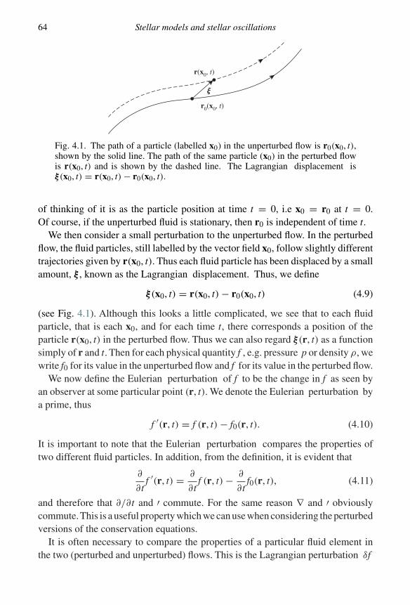
64 Stellar models and stellar oscillations
r(x0, t)
r0(x0, t)
Fig. 4.1. The path of a particle (labelled x0) in the unperturbed flow is r0(x0, t),shown by the solid line. The path of the same particle (x0) in the perturbed flowis r(x0, t) and is shown by the dashed line. The Lagrangian displacement isξ(x0, t) = r(x0, t) − r0(x0, t).
of thinking of it is as the particle position at time t = 0, i.e x0 = r0 at t = 0.Of course, if the unperturbed fluid is stationary, then r0 is independent of time t.
We then consider a small perturbation to the unperturbed flow. In the perturbedflow, the fluid particles, still labelled by the vector field x0, follow slightly differenttrajectories given by r(x0, t). Thus each fluid particle has been displaced by a smallamount, ξ , known as the Lagrangian displacement. Thus, we define
ξ(x0, t) = r(x0, t) − r0(x0, t) (4.9)
(see Fig. 4.1). Although this looks a little complicated, we see that to each fluidparticle, that is each x0, and for each time t, there corresponds a position of theparticle r(x0, t) in the perturbed flow. Thus we can also regard ξ(r, t) as a functionsimply of r and t. Then for each physical quantity f , e.g. pressure p or density ρ, wewrite f0 for its value in the unperturbed flow and f for its value in the perturbed flow.
We now define the Eulerian perturbation of f to be the change in f as seen byan observer at some particular point (r, t). We denote the Eulerian perturbation bya prime, thus
f ′(r, t) = f (r, t) − f0(r, t). (4.10)
It is important to note that the Eulerian perturbation compares the properties oftwo different fluid particles. In addition, from the definition, it is evident that
∂
∂tf ′(r, t) = ∂
∂tf (r, t) − ∂
∂tf0(r, t), (4.11)
and therefore that ∂/∂t and ′ commute. For the same reason ∇ and ′ obviouslycommute.This is a useful property which we can use when considering the perturbedversions of the conservation equations.
It is often necessary to compare the properties of a particular fluid element inthe two (perturbed and unperturbed) flows. This is the Lagrangian perturbation δf
4.3 Eulerian and Lagrangian perturbations 65
defined by
δf (x0, t) = f (x0, t) − f0(x0, t), (4.12)
or equivalently
δf (r, t) = f (r, t) − f0(r0, t), (4.13)
where we recall that r = r0 + ξ .The Eulerian and Lagrangian perturbations are therefore related by the exact
expression
δf = f ′ + [ f0(r, t) − f0(r0, t)]. (4.14)
Using a Taylor series we may write
f0(r, t) = f0(r0, t) + ξ · ∇f0 + O(ξ2). (4.15)
Now to first-order in ξ we have f ≈ f0. This gives the basic result
δf = f ′ + ξ · ∇f (4.16)
to first order in ξ . We note that, since the Lagrangian perturbation δ comes fromconsidering the same fluid element, it is evident that the procedure of forming theLagrangian perturbation commutes with the Lagrangian derivative, that is
D
Dt(δf ) = δ
(Df
Dt
). (4.17)
In addition, we need to add the warnings that ′ does not commute with D/Dt andthat δ commutes neither with ∂/∂t nor with ∇.
4.3.1 The perturbed velocity
In the above we have looked at expressions for the perturbations of scalar fluidquantities such as pressure and density. We need to take a little bit more carewhen considering perturbations of the velocity itself, and in particular the relationsbetween these and the Lagrangian perturbation ξ . We begin by noting that, for afluid particle in the perturbed flow with trajectory r(t), the (perturbed) fluid velocityis given by
u(r, t) = DrDt
. (4.18)
Similarly, for a fluid particle in the unperturbed flow with trajectory r0(t), the(unperturbed) fluid velocity is given by
u0(r0, t) = Dr0
Dt. (4.19)
66 Stellar models and stellar oscillations
Then, taking the difference, we have by definition that
δu = u(r, t) − u0(r0, t). (4.20)
Noting that r = r0 + ξ , we see from the definition (eq. (1.19)) of the Lagrangianderivative that
δu = ∂ξ
∂t+ u · ∇ξ (4.21)
to first order in ξ .Now, since by definition
u′ = u(r, t) − u0(r, t), (4.22)
and since, as we have shown (to first order)
δu = u′ + ξ · ∇u, (4.23)
we obtain finally the expression for the Eulerian velocity perturbation, valid tofirst order in ξ :
u′ = ∂ξ
∂t+ u · ∇ξ − ξ · ∇u. (4.24)
If the unperturbed fluid is at rest, then these considerations are not really necessaryand we have simply that δu = u′ = u = dξ/dt = ∂ξ/∂t.
4.4 Adiabatic perturbations – a variational principle
We are interested in deciding whether stars are stable against perturbations ofvarious types. In principle we could explicitly solve the equations governing allpossible perturbations of these types and see if any of the solutions grow withoutlimit anywhere. Thus we need to know the global behaviour of the perturbations.A more convenient way of keeping track of this is to derive a variational principle.This involves an integral over the whole region of the fluid we are considering, andthus encapsulates the global information we require in a simple way. Deriving avariational principle involves some effort, but the payoff is that we can readily useit to decide the global stability of all perturbations in a straightforward manner.
We consider a fluid initially in hydrostatic equilibrium and subject to fixedgravity. In line with our philosophy of keeping things as simple as possiblewhile retaining the essential physics, we assume a plane-parallel configurationin Cartesian coordinates. Then gravity is given by g = (0, 0, −g) = −∇�, where� is the gravitational potential, which we take to be fixed. Thus the unperturbedconfiguration satisfies following the equation:
∇p = −ρ∇�. (4.25)
4.4 Adiabatic perturbations – a variational principle 67
In the initial configuration the pressure p(z) and density ρ(z) are just functions ofz, and the velocity is zero. This implies that the perturbed velocity u is a first-orderperturbed quantity, and we have u = ∂ξ/∂t.
Then to first-order in perturbed quantities, the mass conservation equation,
∂ρ
∂t+ div(ρu) = 0, (4.26)
becomes
∂ρ′
∂t+ div(ρu) = 0, (4.27)
which we can integrate once with respect to time to yield
ρ′ + div(ρξ) = 0. (4.28)
Similarly, the momentum conservation equation,
ρ∂u∂t
+ ρu · ∇u = ∇p − ρ∇�, (4.29)
becomes
ρ∂2ξ
∂t2= −∇p′ − ρ′∇�. (4.30)
Note here that since u is already a first-order quantity, the second term on the l.h.s.is second-order and so negligible, and also note that since gravity is fixed we canomit the term −ρ∇�′.
We consider adiabatic perturbations. This means that each fluid elementconserves its entropy as it moves, and further that the perturbation itself doesnot change the entropy of individual fluid elements. This is expressed most clearlyby writing (in terms of the Lagrangian perturbation)
δ
(p
ργ
)= 0, (4.31)
or equivalently
δp = γ p
ρδρ. (4.32)
In terms of Eulerian perturbations, we have seen that we may write this asfollows:
p′ + ξ · ∇p = γ p
ρ[ρ′ + ξ · ∇ρ]. (4.33)
Thus we have an expression for the Eulerian pressure perturbation as follows:
p′ = γ p
ρρ′ − ξ ·
{∇p − γ p
ρ∇ρ
}. (4.34)
68 Stellar models and stellar oscillations
We could now substitute eq. (4.28) for ρ′ and eq. (4.34) for p′ into eq. (4.30),and use eq. (4.25) describing the original equilibrium to give an equation solely interms of the Lagrangian fluid perturbation ξ . For any given initial perturbation ξ ,this equation would describe the time evolution of that perturbation. But it is moreuseful at this stage to look for more general properties of the perturbed flow.
Since the original configuration was independent of time t, we may replace thedifferential equation by an algebraic one, just as we did in Chapter 2, by taking theFourier transform of the equation with respect to t. As we remarked earlier, this isequivalent to writing
ξ ∝ exp(iωt). (4.35)
When we do this, the full equation becomes
−ρω2ξ = ∇[γ p
ρdiv(ρξ)
]+ ∇
[ξ ·(
∇p − γ p
ρ∇ρ
)]− 1
ρ∇p div(ρξ).
(4.36)
Note that now ξ represents the Fourier transform of the Lagrangian perturbationwith respect to time, and is in general a complex vector depending on ω andposition r.
We now look for general properties of this equation. To do this we multiply bothsides by the complex conjugate quantity ξ∗ and integrate over all space (or, in fact,since ρ vanishes outside the fluid, over all of the fluid).
The l.h.s. of the equation now becomes
LHS = −ω2I , (4.37)
where I is a real, positive definite quantity given by
I =∫
Vρξ∗ · ξ dV . (4.38)
On the r.h.s. we first gather together the terms with a factor of γ . Simplifying,we obtain
RHS1 =∫
Vξ∗ · ∇[γ p divξ ] dV . (4.39)
We can now integrate this expression by parts. Assuming that the perturbationvanishes on the boundary, we obtain
RHS1 = −∫
Vγ p divξ divξ∗ dV. (4.40)
We can tidy up the rest of the terms on the r.h.s. (i.e. those independent of γ ) togive us two quantities
A = ∇(ξ · ∇p) − ∇p divξ (4.41)
4.4 Adiabatic perturbations – a variational principle 69
and
B = −∇p(ξ · ∇ ln ρ). (4.42)
We take each of these in turn and apply the same procedure as before. From A,integrating the first term by parts and using the same boundary condition that theperturbation vanishes at the boundary, we obtain
RHSA = −∫
VdV {∇p · [ξdivξ∗ + ξ∗divξ ]}. (4.43)
And from B we obtain
RHSB = −∫
VdV {(ξ∗ · ∇p)(ξ · ∇ ln ρ)}. (4.44)
But since the original configuration was plane-parallel, so that
∇p = −|∇p|z, (4.45)
and
∇ ln ρ = −|∇ ln ρ|z, (4.46)
where z is the unit vector in the z-direction, we can rewrite this in more symmetricalfashion as follows:
RHSB =∫
VdV {(∇p · ∇ ln ρ)(z · ξ∗)(z · ξ)}. (4.47)
Gathering all these expressions together, the transformed eq. (4.36) becomes simply
ω2I = K , (4.48)
where the quantity I is defined above and the quantity K is defined as follows:
K =∫
VdV {γ p divξ divξ∗ + ∇p · [ξ divξ∗ + ξ∗divξ ]
+ (∇p · ∇ ln ρ)(z · ξ∗)(z · ξ)}. (4.49)
4.4.1 Implications
The work going into producing eq. (4.49) now allows us to derive a number ofresults.
First, by construction, it is clear that both I and K are real quantities becauseboth are unchanged by replacing ξ ↔ ξ∗. Further we can see that I is positivedefinite. This implies that ω2 is real. Thus either ω2 > 0 and the perturbationsare oscillatory, or ω2 < 0 and the perturbations are exponential, with one growing,and hence unstable, solution.
70 Stellar models and stellar oscillations
Second, since
ω2 = K[ξ ]I [ξ ] , (4.50)
we can see that this is a Sturm–Liouville problem. There is an extensive theory ofsuch problems, treated at length in books on differential equations. In particular,one can always rewrite the problem as a variational principle . Here this means thatthe problem is equivalent to choosing a solution ξ i which minimizes the quantity
F[ξ ] = K[ξ ]I [ξ ] . (4.51)
The resulting quantity ξ i is then an eigensolution to the original perturbationequations, and the corresponding eigenvalue is given by
ω2i = F[ξ i]. (4.52)
We also know that the eigenfunctions are orthogonal.Third, since ω2 is real, it follows that if we consider a continuous series of
initial configurations which differ from each other by changing some parameter ina continuous fashion, then the change from stability to instability must occur whenω2 passes through zero. That is, the ‘exchange of stabilities’ occurs when ω2 = 0.
4.4.2 Implication for stability
We have noted that, loosely, stability depends on whether ω2 is greater or lessthan zero. But of course ω2 depends on ξ . We now look in a little more detail tosee how the above analysis can give us a criterion for the stability of the originalconfiguration.
We started with an equation (eq. (4.30)) of the following form (after substitution):
ρ∂2ξ
∂t2= Lξ , (4.53)
where ξ is a function of r and t, and L is a time-independent linear operator. Thismeans that
∂
∂tLξ = L
∂ξ
∂t. (4.54)
In addition, a slight modification of the analysis at the beginning of this section,replacing ξ∗ by η, shows that the operator L is symmetric, by which we mean that∫
Vξ(Lη) dV =
∫V
η(Lξ) dV (4.55)
for any two quantities ξ(r, t) and η(r, t).We can now find criteria for stability and instability.
4.4 Adiabatic perturbations – a variational principle 71
4.4.2.1 Stability
We show here that if the quantity
W (t) =∫
Vξ(Lξ) dV (4.56)
is negative for all non-zero ξ , then the configuration is stable. To keep the algebrasimple, we assume that ξ is real. If this does not hold, then the same analysis resultsby setting one of the ξ on the r.h.s. to ξ∗ and then taking the real part.
We note first that, since L is symmetric,
dW
dt= 2
∫V
∂ξ
∂t· (Lξ) dV . (4.57)
We then consider the quantity
K(t) = 1
2
∫V
ρ∂ξ
∂t· ∂ξ
∂tdV , (4.58)
which represents the kinetic energy of the perturbation. It is clearly positivedefinite. Evidently,
dK
dt=∫
Vρ
∂2ξ
∂t2· ∂ξ
∂tdV , (4.59)
and hence, using eqs. (4.53) and (4.57), we deduce that
dK
dt= 1
2
dW
dt. (4.60)
Integrating with respect to t, this then implies that
2K(t) = W (t) + 2E, (4.61)
where E is a constant. Since by assumption W (t) < 0 at all times t, we conclude that
K(t) < E (4.62)
at all times t. Thus the kinetic energy of the perturbation is bounded above, andthe configuration is stable.
4.4.2.2 Instability
We now show that if we can find some function η(r) such that
W0 =∫
Vη · (Lη) dV > 0, (4.63)
then the original configuration is unstable.We begin by defining ω0 > 0 by
W0 = ω20
∫V
η · η dV . (4.64)
72 Stellar models and stellar oscillations
We then consider a perturbation of the fluid configuration such that at time t = 0the displacement is given by
ξ(r, 0) = η(r) (4.65)
and the perturbed velocity is given by
∂ξ
∂t= ω0η. (4.66)
Then, by construction, at time t = 0, and therefore for all time t > 0, we have2K = W and hence E = 0.
We now consider the quantity I(t) defined by
I(t) =∫
Vρξ · ξ dV . (4.67)
Differentiating twice, we find simply that
1
2
d2I
dt2= 2K + W , (4.68)
and so in this case
d2I
dt2= 8K . (4.69)
We now use the Schwarz inequality in the following form:(∫V
ρξ · ∂ξ
∂tdV
)2
≤(∫
Vρξ · ξ dV
)(∫V
ρ∂ξ
∂t· ∂ξ
∂tdV
)(4.70)
to show that (1
2
dI
dt
)2
≤ I × 2K . (4.71)
We then substitute for K from eq. (4.69) to show that
d
dt
(1
I
dI
dt
)≥ 0. (4.72)
Because of the initial conditions we have chosen for the perturbation, we knowthat at t = 0, I(dI/dt) = 2ω0 > 0. We therefore conclude that, for all times t ≥ 0,
1
I
dI
dt≥ 2ω0, (4.73)
and hence that
I(t) ≥ I(0) exp(2ω0t), (4.74)
and that the perturbation grows exponentially without limit.
4.5 The Schwarzschild stability criterion 73
4.4.2.3 Stability criterion
We conclude from all this that a necessary and sufficient condition for stability isthat W defined in eq. (4.56) is negative for all vector fields ξ . This is the globalcriterion we have been seeking, and we can use it to decide stability.
4.5 The Schwarzschild stability criterion
As an example we demonstrate how the above analysis gives a criterion for thestability of a fluid against convection.
We start from the equation describing the evolution of the perturbation,eq. (4.30):
ρ∂2ξ
∂t2= −∇p′ − ρ′∇�. (4.75)
The equation which describes the adiabaticity of the perturbations, eq. (4.34) canbe written as follows:
ρ′ = ρ
γ pp′ − ρ(A · ξ), (4.76)
where the quantity A is given by
A = 1
ρ∇ρ − 1
γ p∇p. (4.77)
We now recall that the r.h.s. of eq. (4.75) is just Lξ . We then multiply this equationby ξ , use eq. (4.76) to eliminate ρ′, recall that ∇� = −∇p/ρ and integrate overthe volume of the fluid, to obtain∫
Vξ · (Lξ) dV =
∫V
dV
{p′divξ + p′
γ p(ξ · ∇p) − (ξ · ∇p)(A · ξ)
}, (4.78)
where we have integrated the first term by parts and assumed that the perturbationvanishes on the boundary.
We can simplify this by using the mass conservation equation in thefollowing form:
divξ = −ρ′
ρ− 1
ρξ · ∇ρ, (4.79)
to replace divξ in the first term on the r.h.s., and by then using eq. (4.76) to eliminateρ′. Then two of the terms cancel and we obtain finally∫
Vξ · (Lξ) dV = −
∫V
dV
{(p′)2
γ p+ (ξ · ∇p)(A · ξ)
}. (4.80)
74 Stellar models and stellar oscillations
Now by the definition of A in eq. (4.77) we see that ∇p and A are either parallelor anti-parallel. We also note that, since the entropy S ∝ ln(p/ργ ),
A = − 1
γ∇S. (4.81)
Then, if entropy increases upwards, so that ∇p · A > 0, we have that W > 0 forall ξ , and therefore stability. On the other hand, if somewhere in the fluid entropyincreases downwards, so that in some region of the fluid ∇p · A < 0, then we canchoose a vector function ξ which is sufficiently concentrated in that region thatW < 0, and we have instability.
We conclude that the fluid is stable if and only if the entropy and pressuregradients are anti-parallel. Or, since in equilibrium gravity is anti-parallel to thepressure gradient, we conclude that the fluid is unstable if and only if entropydecreases downwards in the direction of gravity. This is the Schwarzschild criterionfor convective instability. It implies, loosely speaking, that the fluid is stable if thehotter (higher entropy ) fluid is on top and that convection sets in if the hotter(higher entropy) fluid is underneath. This corresponds directly to what we seewhen heating water from below, for example in a saucepan. In stars we often havestability against convection, even though the temperature decreases outwards. Thisis because the decrease in density ρ is sufficiently rapid that the specific entropy∝ ln(p ρ−γ ) nevertheless increases outwards.
We can understand the Schwarzschild criterion by a simple physical argument,where we consider a fluid element displaced vertically upwards. Once it comesinto pressure equilibrium with its new surroundings, we can see that it will fallback (stability against convection) provided that its density ρ is higher thanits surroundings, i.e. provided that its entropy is lower than its surroundings.Assuming that the displacement was adiabatic, i.e. rapid enough for the elementto conserve its entropy, this amounts to requiring entropy to decrease outwards inthe unperturbed star, as the Schwarzschild criterion requires. In regions of starswhere the Schwarzschild criterion fails, i.e. where entropy increases outwards,convection acts as an extremely efficient means of transporting energy out throughthe star. In fact, it is so efficient that the Schwarzschild criterion has only to bevery slightly violated for the convection to carry the entire luminosity of the star.This is very convenient, for in many cases one can replace a detailed description ofthe convection with the simple condition that the entropy is constant, i.e. that theSchwarzschild criterion is only marginally violated.
4.6 Further reading
A description of the construction of models of stars is given in Clayton (1983,Chap. 6). Further clarification about the treatment of Eulerian and Lagrangian
4.7 Problems 75
perturbations is given in Cox (1980, Chap. 5), who also discusses the Schwarzschildstability criterion (Chap. 17).
4.7 Problems
4.7.1 The equations governing the adiabatic perturbations, ξeiωt , of a spherical star canbe manipulated to yield the following expression:
I [ξ ]ω2 = K[ξ ], (4.82)
where
I =∫
ρξ∗ · ξ dV . (4.83)
Show that taking account of the self-gravity of the perturbation gives a term ofthe form −ρ∇�′ in the equations of motion. Show that combining this with thelinearized version of Poisson’s equation produces the following term:
G∫ ∫
div[ρ(r)ξ(r)]div′[ρ(r′)ξ∗(r′)]|r − r′| dV dV ′ (4.84)
in K[ξ ].4.7.2 A spherically symmetric star, of radius R and mass M , undergoes small radial
pulsations. The radial displacement vector is ξ = rη(r)r. The pulsation frequency ω
satisfies the equation
ω2I = K , (4.85)
where
I =∫ R
0ρr4η2 dr (4.86)
and
K =∫ R
0
{γ pr4
(dη
dr
)2
− r3η2 d
dr[(3γ − 4)p]
}dr. (4.87)
If
m(r) =∫ r
04πr2ρ dr, (4.88)
show that, for a physically reasonable stellar density distribution ρ(r),
m
r3>
M
R3. (4.89)
If γ is independent of radius, deduce that
ω2 > (3γ − 4)GM
R3. (4.90)
(See Cox (1980, Chap. 8).)
76 Stellar models and stellar oscillations
4.7.3 The equation of motion for a body of fluid in volume V , bounded by surface S, hasthe following form:
ρd2
dt2(xi) = − ∂
∂xi
(p + 1
2µB2)
− ρ∂�
∂xi+ ∂
∂xk(BiBk). (4.91)
Use this to prove the scalar virial theorem, which states that
1
2
d2I
dt2= 2T + W + 3(γ − 1)U + M + S, (4.92)
where
I =∫
Vr · rρ dV , (4.93)
M is the magnetic energy defined by
M = 1
2
∫V
B2 dV , (4.94)
T is the kinetic energy,
T = 1
2
∫V
(dxi
dt
dxi
dt
)ρ dV , (4.95)
W is the gravitational energy ,
W = 1
2
∫V
ρ� dV = −G∫
Vρr · ∇� dV , (4.96)
and U is the internal (thermal) energy,
U = 1
γ − 1
∫V
p dV , (4.97)
and the surface integral S is given by
S = −∫
S
(p + 1
2B2)
r · dS + 1
µ
∫(r · B) B · dS. (4.98)
Assume p = (γ − 1)ρe, with γ constant. (See Sturrock (1994, Chap. 12).)4.7.4 Consider a fluid at rest, occupying volume V , with pressure distribution p(r), density
distribution ρ(r) in a fixed gravitational field g = −∇�(r) and permeated by amagnetic field B(r). Write down the equation describing the hydrostatic equilibrium.
The configuration undergoes a small oscillatory perturbation with displacementvector ξ(r)eiωt and with div ξ = 0. If the perturbation to the magnetic field isb(r)eiωt , show that
bi = Bj∂ξi
∂xj− ξj
∂Bi
∂xj(4.99)
and deduce that div b = 0.
4.7 Problems 77
Assuming (without proof) that all surface integrals vanish when integrating byparts show that
ω2∫
Vρ ξ∗
i ξj dV =∫
Vξ∗
i ξj∂2
∂xi∂xj
[p + 1
2B2]
dV +∫
Vρ ξ∗
i ξj∂2�
∂xi∂xjdV
+∫
V
(Bj
∂ξ∗i
∂xj
)(Bk
∂ξi
∂xk
)dV
and hence that ω2 is real.Now consider a particular configuration in which the fluid is vertically stratified
with p(z) and ρ(z) in a constant gravitational field g = (0, 0, −g), and with ahorizontal magnetic field B = (B(z), 0, 0). Write down the equilibrium equationfor this configuration.
By considering the perturbation ξ = (0, 0, sin ky) in the above expression,comment on how stability depends on the sign of ∂ρ/∂z.
Comment also on the stability properties of perturbations of the form ξ =(0, 0, sin kx).
(Ageneral variational principle for treating the stability of hydromagnetic systemsis presented by Chandrasekhar (1961, Chap. IV).)
5
Stellar oscillations – waves in stratified media
In the previous chapter we showed that if a star is stable it oscillates about itsequilibrium configuration when perturbed. To do this we looked at the globalproperties of the whole star. We showed that the star acts like an organ pipe inthat it oscillates in a distinct set of modes with a distinct set of frequencies. Butto investigate the details of the oscillation modes of the star, we need to lookat the details of how the oscillations propagate through the star. In line with ourphilosophy expressed previously, we shall simplify matters by only considering flat‘stars’, or equivalently we can think of the analysis as applying to a plane-parallelatmosphere, whose vertical thickness is small compared with the star’s radius.
To understand the physics of the oscillations, we need to ask what the restoringforces are. That is, if we perturb the fluid, what tries to push it back to where it was?We have so far come across two types of restoring force in non-magnetic media,and we can expect both to operate in a star. They are pressure and buoyancy.
(i) Pressure. If we compress a fluid element, we increase its pressure, and this increaseproduces a restoring force. The resulting oscillations are sound waves, with localspeed cs = √
γ p/ρ. Oscillation modes in which pressure is the main restoring forceare called p-modes.
(ii) Buoyancy, or gravity. In a horizontally stratified fluid with gravity g = (0, 0, −g), wehave seen that stability requires that the quantity A (see eq. (4.77)),
A = 1
ρ
dρ
dz− 1
γ p
dp
dz, (5.1)
is negative. Such a fluid is stably stratified. If we perturb it in the vertical direction,gravity acts on the fluid elements to try to restore them to their original positions. It isclear that we do not need the fluid to be compressible for this to happen. A simple wayto envisage these waves is to regard them as analogous to water waves on the surface ofa pond or the sea. Then it is clear that a vertical displacement of the surface undergoesa restoring force due to gravity. From the physical quantities g and A, we can define a
78
5.1 Waves in a plane-parallel atmosphere 79
relevant frequency N , known as the Brunt–Väisälä frequency, given by
N 2 = −gA. (5.2)
For these oscillations gravity is the main restoring force and they are known as g-modes. Note that N is real if and only if A < 0, i.e. the Schwarzschild criterion issatisfied. Thus g-modes propagate freely only in radiative regions of the star and areevanescent in convective ones.
We now investigate the properties of these modes of oscillation in more detail.
5.1 Waves in a plane-parallel atmosphere
We consider a horizontally stratified fluid with constant gravity g = (0, 0, −g). Thusin hydrostatic equilibrium the unperturbed values of p(z) and ρ(z) are related by
dp
dz= −ρg. (5.3)
We first perturb the equation of mass conservation, which is
∂ρ
∂t+ u · ∇ρ + ρ div u = 0, (5.4)
to obtain, in terms of first-order Eulerian perturbed quantities,
∂ρ′
∂t+ u · ∇ρ + ρ div u = 0. (5.5)
Similarly, we perturb the momentum equation,
∂u∂t
+ u · ∇u = − 1
ρ∇p + g, (5.6)
to obtain∂u∂t
= ρ′
ρ2∇p − 1
ρ∇p′. (5.7)
Note that we have assumed that gravity is fixed, so that g′ = 0.Because the unperturbed fluid is independent of time, and of the horizontal
coordinates x and y, we can Fourier transform the equations with respect tothese quantities, or equivalently we write all perturbed quantities in the form
p′ ∝ exp{i(ωt − kxx − kyy)}. (5.8)
Note that now the perturbed quantities are still functions of the vertical coordinatez. Thus, for example, we regard the pressure perturbation as having the functionalform p′ = p′(z; ω, kx, ky). In addition, we shall write the components of theperturbed velocity in the following form:
u = (u, v, w). (5.9)
80 Stellar oscillations – waves in stratified media
When we do this, eq. (5.5) becomes
iωρ′ + wdρ
dz+ ρ
{−ikxu − ikyv + dw
dz
}= 0. (5.10)
Similarly, the three components of eq. (5.7) become
iωu = 1
ρikxp′, (5.11)
iωv = 1
ρikyp′ (5.12)
and
iωw = ρ′
ρ2
dp
dz− 1
ρ
dp′
dz. (5.13)
We now need to provide a relationship between p′ and ρ′. As before we shallassume that the oscillations are adiabatic so that energy is conserved. This impliesthat
∂
∂t
(p
ργ
)+ u · ∇
(p
ργ
)= 0. (5.14)
The first-order Eulerian perturbation of this equation is given by
1
ργ
∂p′
∂t− γ p
ρ
1
ργ
∂ρ′
∂t+ w
d
dz
(p
ργ
)= 0. (5.15)
Then applying Fourier transforms to this equation yields the following result:
iωp′ − iωγ p
ρρ′ + ργ w
d
dz
(p
ργ
)= 0. (5.16)
It is now more convenient to work in terms of the quantity h′ = p′/ρ, which can bethought of as being related to the perturbation to the specific enthalpy h = ∫
dp/ρ.Then eq. (5.11) becomes
u = kxh′
ω(5.17)
and eq. (5.12) becomes
v = kyh′
ω. (5.18)
We use these to eliminate the horizontal velocity components u and v from theanalysis. Substituting for u and v, eq. (5.10) becomes
iωρ′
ρ+ w
1
ρ
dρ
dz+ dw
dz− i
(k2x + k2
y )h′
ω= 0. (5.19)
We replace p′ with h′ in eq. (5.13) to yield
iωw = ρ′
ρ2
dp
dz− dh′
dz− 1
ρ
dρ
dzh′ (5.20)
5.1 Waves in a plane-parallel atmosphere 81
and in eq. (5.16) to yield
γ p
ρ
ρ′
ρ= h′ − w
iργ−1
ω
d
dz
(p
ργ
). (5.21)
We now have three equations for the three variables ρ′/ρ, h′ and w. We note thatthe equations do not involve derivatives of ρ′/ρ. Thus we can use eq. (5.21) tosubstitute for ρ′/ρ in the other two equations.
Substituting in eq. (5.20), we obtain, after a little algebra,
γ p
ρ
dh′
dz− ργ−1 d
dz
(p
ργ
)h′ = −iw
{ω
γ p
ρ− gργ−1
ω
d
dz
(p
ργ
)}, (5.22)
where we have used the equilibrium condition that
g = − 1
ρ
dp
dz. (5.23)
Then, using the fact that the expression for A can be rewritten in the following form:
A = − d
dz
(p
ργ
)× ργ
γ p, (5.24)
we may write the equation as follows:
dh′
dz+ Ah′ = −iw
{ω + Ag
ω
}. (5.25)
Writing eq. (5.21) asρ′
ρ=(
ρ
γ p
)h′ + iwA
ω, (5.26)
we substitute this into eq. (5.19) to obtain an equation for dw/dz in the followingform:
dw
dz− g
c2s
w + ih′[
ω
c2s
− k2⊥ω
]= 0. (5.27)
Here we have used the notation that the horizontal component of the wave vector,k⊥, is given by
k2⊥ = k2x + k2
y . (5.28)
Equations (5.25) and (5.27) describe the oscillations. We can put them intoneater form by recalling that N 2 = −Ag and that the vertical displacement of afluid element, ξz, is given by
w = iωξz. (5.29)
Using this, we write the equations in the final form:
dξz
dz− g
c2sξz + 1
c2s
[1 − k2⊥c2
s
ω2
]h′ = 0 (5.30)
82 Stellar oscillations – waves in stratified media
anddh′
dz− N 2
gh′ + (N 2 − ω2)ξz = 0. (5.31)
5.1.1 Local analysis
For any plane-parallel distribution of density and pressure we can now use these twoequations to find the oscillation frequencies, ω, and the structure of the oscillationmodes. We do this for a particular set of oscillations in Section 5.2. Before we dothat, however, it is instructive to look more generally at the kinds of oscillationsthat can propagate and to get a feel for the physics involved.
We undertake what is known as a local analysis and obtain a local dispersionrelation, i.e. the relation between wavelength and frequency or wavenumber. Weconsider waves which have a vertical wavelength which is very small compared tothe vertical scaleheight of the background distribution. To do this we set
ξz ∝ exp(ikzz) (5.32)
andh′ ∝ exp(ikzz), (5.33)
where kz � g/c2s . In this approximation, eq. (5.30) becomes
ikzξz + 1
c2s
[1 − k2⊥c2
s
ω2
]h′ = 0 (5.34)
and eq. (5.31) becomes
(N 2 − ω2)ξz + ikzh′ = 0. (5.35)
These are two linear homogeneous equations, and so for a non-trivial solutionwe require the determinant of coefficients to vanish. This yields the followingcondition:
k2z + 1
c2s(N 2 − ω2)
[1 − k2⊥c2
s
ω2
]= 0. (5.36)
This is the local dispersion relation, which can be written as a quadratic for ω2 inthe following form:
ω4 − (N 2 + k2c2s )ω
2 + N 2k2⊥c2s = 0, (5.37)
where k is the full wavevector given by k2 = k2⊥ + k2z .
In Fig. 5.1, we consider the local propagation properties of the oscillations inthe (k2⊥, ω2)-plane. For mode propagation to take place we need both k2⊥ ≥ 0 forhorizontal propagation and k2
z ≥ 0 for vertical propagation. In addition, we need
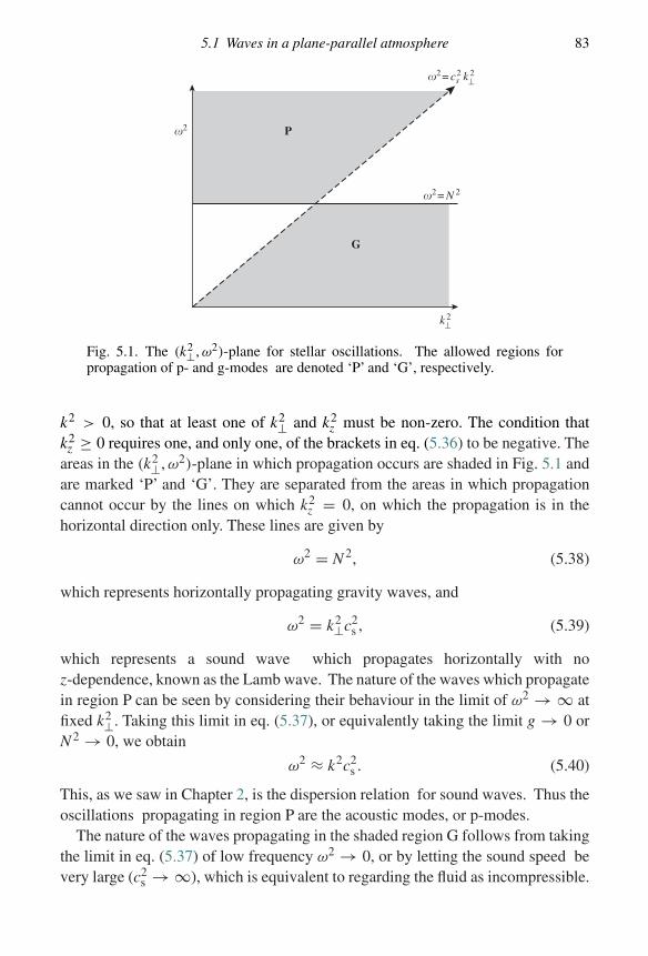
5.1 Waves in a plane-parallel atmosphere 83
�2 P
G
�2 = cs2 k⊥
2
�2 = N 2
k⊥2
Fig. 5.1. The (k2⊥, ω2)-plane for stellar oscillations. The allowed regions forpropagation of p- and g-modes are denoted ‘P’ and ‘G’, respectively.
k2 > 0, so that at least one of k2⊥ and k2z must be non-zero. The condition that
k2z ≥ 0 requires one, and only one, of the brackets in eq. (5.36) to be negative. The
areas in the (k2⊥, ω2)-plane in which propagation occurs are shaded in Fig. 5.1 andare marked ‘P’ and ‘G’. They are separated from the areas in which propagationcannot occur by the lines on which k2
z = 0, on which the propagation is in thehorizontal direction only. These lines are given by
ω2 = N 2, (5.38)
which represents horizontally propagating gravity waves, and
ω2 = k2⊥c2s , (5.39)
which represents a sound wave which propagates horizontally with noz-dependence, known as the Lamb wave. The nature of the waves which propagatein region P can be seen by considering their behaviour in the limit of ω2 → ∞ atfixed k2⊥. Taking this limit in eq. (5.37), or equivalently taking the limit g → 0 orN 2 → 0, we obtain
ω2 ≈ k2c2s . (5.40)
This, as we saw in Chapter 2, is the dispersion relation for sound waves. Thus theoscillations propagating in region P are the acoustic modes, or p-modes.
The nature of the waves propagating in the shaded region G follows from takingthe limit in eq. (5.37) of low frequency ω2 → 0, or by letting the sound speed bevery large (c2
s → ∞), which is equivalent to regarding the fluid as incompressible.
84 Stellar oscillations – waves in stratified media
In this limit the dispersion relation, eq. (5.37), becomes
ω2 ≈ N 2 k2⊥k2
. (5.41)
From the presence of the N 2 term, we see that here the restoring force is gravity.These are the gravity waves, or g-modes. We note that the waves need non-zero k⊥in order to propagate. Thus, these waves cannot propagate purely vertically. Thesewaves are analogous to surface waves on water, but propagate within the body ofthe fluid because of the local buoyancy. They are also known as internal buoyancywaves.
The propagation properties of these waves are peculiar. The phase velocity , i.e.the direction and speed at which the wave crests travel, is in the direction of thewavevector and is given by
vs = ω
kk. (5.42)
However, the group velocity of the waves, which is the direction and speed atwhich the waves transport energy and momentum, is given by vg = ∂ω/∂k. Usingeq. (5.41) we find that for these waves
vg = ωkz
k2⊥k ∧ (k ∧ z). (5.43)
From this we see that the group velocity is perpendicular to the phase velocity!Thus energy and momentum are carried parallel to the wave crests.
5.2 Vertical waves in a polytropic atmosphere
We now consider an example of how to use the wave equations we derived above tocompute a set of oscillation modes in a particular distribution of fluid. We considera fluid which is horizontally stratified, with constant gravity g = (0, 0, −g). Wetake the equation of state of the unperturbed fluid to be polytropic so that theunperturbed values of p(z) and ρ(z) are related by
p = Kρ1+1/m, (5.44)
where K is a constant, and m > 0 is also a constant, known as the polytropic index.We consider only those modes which propagate in the vertical direction. These arethe equivalent of radial oscillation modes in a star. From our discussions abovewe already know that we expect these modes to be p-modes, because the g-modescannot propagate vertically.
5.2 Vertical waves in a polytropic atmosphere 85
5.2.1 Equilibrium distribution
We must first determine the pressure and density distributions in the fluid. To dothis we combine the equation of hydrostatic equilibrium,
dp
dz= −gρ, (5.45)
with the polytropic equation of state, eq. (5.44), to find that
ρ(z) =[
g
(m + 1)K
]m
(−z)m. (5.46)
Here we note that this only describes the density in the region z < 0. We take thedensity to be zero in the region z > 0, so that the fluid represents a portion of astellar atmosphere and has a surface which we have chosen to be at z = 0. Foralgebraic convenience we let x = −z, and thus the edge of the atmosphere is atx = 0 and it extends to positive x. We then find that ρ ∝ xm, pressure p ∝ xm+1
and temperature T ∝ x. Thus the temperature increases linearly with the distancefrom the surface. We also find that the sound speed is given by
c2s = γ g
m + 1x (5.47)
and that the buoyancy, N 2/g = −A, is given by
N 2
g= (γ − 1)m − 1
γ x. (5.48)
We note that the fluid has neutral buoyancy if it has uniform entropy, that is ifγ = 1 + 1/m. And, as we expect from the Schwarzschild criterion (Section 4.5),stability (i.e. N 2 ≥ 0) requires γ ≥ 1 + 1/m.
5.2.2 The governing equation
To look at the details of vertically propagating waves, we set k⊥ = 0 in eqs. (5.30)and (5.31) to obtain
c2s
dξz
dz− gξz + h′ = 0 (5.49)
anddh′
dz− N 2
gh′ + (N 2 − ω2)ξz = 0. (5.50)
We take eq. (5.49) and its derivative to obtain expressions for h′ and dh′/dz in termsof ξz and its first and second derivatives. These we then substitute into eq. (5.50),and use eqs. (5.47) and (5.48), to obtain a second-order differential equation forξz. Setting x = −z, we find the resulting equation:
c2s
d2ξz
dx2+ γ g
dξz
dx+ ω2ξz = 0. (5.51)
86 Stellar oscillations – waves in stratified media
We note that from eq. (5.47) the coefficient of the first term c2s ∝ x. As we
expected for vertically propagating waves, the buoyancy term involving N 2 hasdropped out.
5.2.3 Solution of the equation
We have argued that these oscillation modes must just be p-modes. Thus we expectthe character of the waves to be acoustic waves travelling in a medium in whichthe sound speed changes along the direction of propagation.† Rather than usingthe distance from the top of the atmosphere, x, as the independent variable, it thenmakes sense to use time of travel of acoustic waves from the top of the atmosphere,τ , where
τ =∫ x
0
dx
cs. (5.52)
Using eq. (5.47), we find that the relevant substitution is given by
x = 1
4
(γ g
m + 1
)τ 2. (5.53)
Using this in eq. (5.51), we find that the governing equation becomes
d2ξz
dτ 2+ 2m + 1
τ
dξz
dτ+ ω2ξz = 0. (5.54)
The solution of this equation can be written in terms of Bessel functions:
ξz = τ−m{C1Jm(ωτ) + C2J−m(ωτ)}, (5.55)
where C1 and C2 are constants.From the mathematical point of view, it makes sense to demand that ξz is finite
at the surface τ = 0. Recalling the property of Bessel functions that Jm(Z) ∼ Zm
as Z → 0, we see that this requires C2 = 0. From a physical point of view, thesurface is defined by having zero pressure outside it. Once the surface is oscillating,we require that the pressure remains zero at the new position of the surface. Thuswe require that the Lagrangian perturbation, δp = p′ + ξz(dp/dz), vanishes atz = 0. Note that this is not the same as demanding that p′ vanish there! Noting thatdp/dz = −gρ, this condition becomes
h′ − gξz = 0 (5.56)
† An exactly analogous problem is that of small oscillations of a uniform, vertically hanging chain. Therethe square of the wave speed is proportional to the tension, which increases linearly with distance from thebottom of the chain.
5.4 Problems 87
at z = 0. From eq. (5.49), we see that this is equivalent to the condition that
dξz
dz= 0 (5.57)
at z = 0.† This gives us the same condition as before, namely C2 = 0.Because the problem is linear, the other constant C1 is not defined and merely
represents the magnitude of the oscillations. In a real star we would need to setanother boundary condition at the centre of the star, and this would determine thepossible oscillation frequencies ω. To simulate that here, we take the atmosphereto have a finite depth H at which the base of the atmosphere is fixed.‡ Thus wedemand that ξz = 0 at x = H . If we define τ1 as being the time for a wave topropagate from the top to the bottom of the atmosphere, i.e.
τ1 =∫ H
0
dx
cs, (5.58)
then the oscillation frequencies are given by the condition that ωτ1 = Zi, whereZi, i = 0, 1, 2, . . ., is one of the infinite set of zeros (Z0 < Z1 < Z2 < · · · ) of theBessel function Jm(Z). We see that the boundary conditions have picked out adiscrete set of oscillation frequencies.
5.3 Further reading
The general theory of stellar oscillations can be found in Unno et al. (1979) andCox (1980). Wave propagation in plane-parallel atmospheres is discussed in Lamb(1932, Chap. X). The properties of internal waves in a stratified, incompressiblefluid are discussed by Turner (1973, Chap. 2).
5.4 Problems
5.4.1 A constant gravity, convectively neutral, polytropic, plane-parallel atmosphere hasa zero density surface at x = 0 and a fixed base at x = H . Show that the adiabaticvertical velocity perturbations of the atmosphere form a set of eigenfunctions ofthe form un(x)eiωnt , which satisfy the following orthogonality relation:∫ H
0f (x)un(x)um(x) dx = δmn, (5.59)
where the function f (x) is to be determined.How do we determine the eigenvalues?
† For the problem of the swinging chain, this is simply the condition that the bottom of the chain is free toswing.
‡ For the chain problem, this is equivalent to taking the top of the chain to be fixed.
88 Stellar oscillations – waves in stratified media
5.4.2 A static, gaseous plane-parallel atmosphere rests on a fixed base at z = 0 and issubject to a fixed gravitational field g = (0, 0, −g(z)), where g(z) = �2z and � isa constant. The atmosphere is isothermal, with (isothermal) sound speed cs. Showthat the density structure is of the form (0 ≤ z < ∞)
ρ(z) = ρ0 exp(−z2/2H 2), (5.60)
where ρ0 is the density at z = 0 and H is a constant.The atmosphere is subject to small adiabatic velocity perturbations of the form
u = (0, 0, w(z)eiωt), where ω is the oscillation frequency. What kind of modeswould you expect to find in such an atmosphere, and what kind of modes does thisperturbation represent?
Show that w(z) obeys the following equation:
d2w
dz2− z
H 2
dw
dz+ 1
γ
(ω2
c2s
− 1
H 2
)w = 0, (5.61)
where γ is the usual ratio of specific heats.By considering a series solution about z = 0, or otherwise, show that the oscillation
modes wn(z) with finite kinetic energy E = ∫∞0
12ρw2 dz take the form of
polynomials of degree N = 2n + 1 for n = 0, 1, 2, . . . . Show that the correspondingoscillation frequencies ωn are given by
ω2n = (γ N + 1)c2
s
H 2. (5.62)
5.4.3 A static polytropic atmosphere subject to uniform gravitational acceleration g = gx(where x is measured downwards) has density and pressure given by
ρ = ρ0
( x
H
)m, p = p0
( x
H
)m+1, (5.63)
below the surface x = 0, where ρ0, p0, and H are positive constants (in general1 + 1/m differs from the adiabatic exponent γ = 1 + 1/n of the gas).
Find the linearized equations for the displacement, density perturbation andpressure perturbation, neglecting self-gravity, and assuming that the displacementhas the following form:
Re[ξ(x) exp(ik · r − iωt)]. (5.64)
Eliminate all variables in terms of the displacement divergence � = ∇ · ξ and obtainthe following equation
zd2�
dx2+ (m + 2)
d�
dx+[
n(m + 1)
n + 1
ω2
gk+(
m − n
n + 1
)gk
ω2− kx
]k� = 0. (5.65)
Make the transformation � = w(x)e−kx and find the solutions of the resultingequation for w as power series in x. Show that the only solutions for which � isfinite at the surface and decays with depth are those for which w is a polynomial in
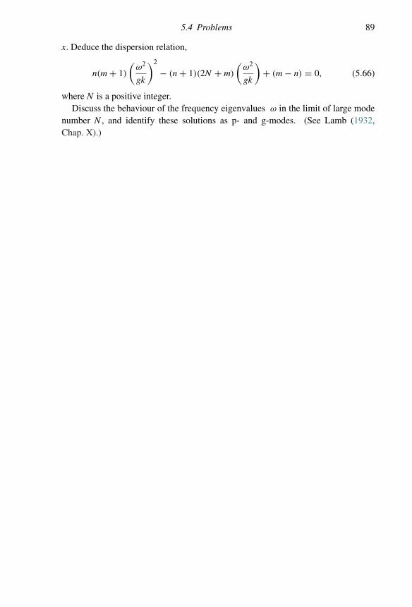
5.4 Problems 89
x. Deduce the dispersion relation,
n(m + 1)
(ω2
gk
)2
− (n + 1)(2N + m)
(ω2
gk
)+ (m − n) = 0, (5.66)
where N is a positive integer.Discuss the behaviour of the frequency eigenvalues ω in the limit of large mode
number N , and identify these solutions as p- and g-modes. (See Lamb (1932,Chap. X).)

6
Damping and excitation of stellar oscillations
In Chapter 5 we considered the various oscillation modes that a star can showwhen perturbed in some way. Many types of star are observed to pulsate. Perhapsthe best known are the class known as Cepheids (after the prototype star δ Cephei).These pulsate primarily in a radial mode, so that we observe the full amplitudeof their oscillations. The period of these oscillations is directly related to thestellar radius, just as the pitch of an organ note is related to the length of the pipeproducing it, the lowest notes coming from the longest pipes. Finding the star’sradius in this way gives a measure of its brightness, so that simply by comparingthe periods of two Cepheids we know their relative brightnesses. Thus, withcareful calibration, measuring the period and the apparent brightness of a Cepheidgives its distance. As Cepheids are bright stars they can be seen in very distantgalaxies and therefore can be used to produce a distance scale of great importance inastronomy.
However, most stars do not show pulsations of readily observable amplitude.This must mean that for most stars any oscillations set in motion by perturbationsreceived during their lives, or in the process of formation, have long since beendamped out in some way. The existence of these damping processes in turn impliesthat if a star does pulsate, an excitation mechanism for these pulsations must beoperating. Typically such mechanisms are not dynamical, such as a stellar collision,but involve physical processes within the star itself. We get considerable insightinto what must be involved in the excitation process by plotting the locations ofknown types of pulsating stars on the Hertzsprung–Russell diagram of luminosityversus effective temperature. Most types of pulsating stars lie in a restricted region(the ‘instability strip’) of this diagram, that is pulsations are favoured in stars witheffective temperatures Te ∼ 6000–10 000 K.
In this chapter we take a brief look at damping and excitation processes in stars.As usual, we do so in a very simplified manner in order to bring out the essentialphysical ideas, without obscuring them with excessive algebraic complexity.
90
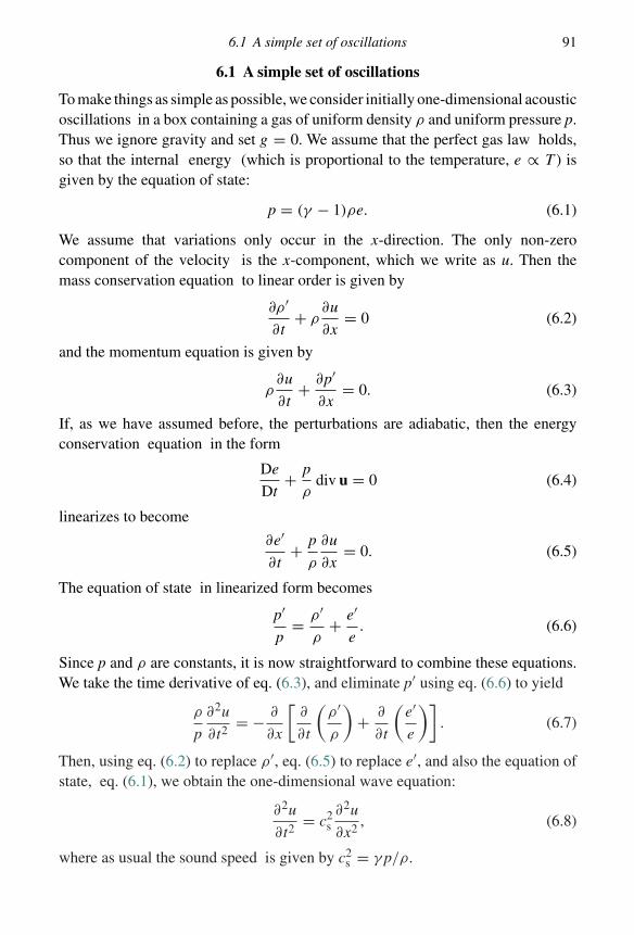
6.1 A simple set of oscillations 91
6.1 A simple set of oscillations
To make things as simple as possible, we consider initially one-dimensional acousticoscillations in a box containing a gas of uniform density ρ and uniform pressure p.Thus we ignore gravity and set g = 0. We assume that the perfect gas law holds,so that the internal energy (which is proportional to the temperature, e ∝ T ) isgiven by the equation of state:
p = (γ − 1)ρe. (6.1)
We assume that variations only occur in the x-direction. The only non-zerocomponent of the velocity is the x-component, which we write as u. Then themass conservation equation to linear order is given by
∂ρ ′
∂t+ ρ
∂u
∂x= 0 (6.2)
and the momentum equation is given by
ρ∂u
∂t+ ∂p′
∂x= 0. (6.3)
If, as we have assumed before, the perturbations are adiabatic, then the energyconservation equation in the form
De
Dt+ p
ρdiv u = 0 (6.4)
linearizes to become
∂e′
∂t+ p
ρ
∂u
∂x= 0. (6.5)
The equation of state in linearized form becomes
p′
p= ρ′
ρ+ e′
e. (6.6)
Since p and ρ are constants, it is now straightforward to combine these equations.We take the time derivative of eq. (6.3), and eliminate p′ using eq. (6.6) to yield
ρ
p
∂2u
∂t2= − ∂
∂x
[∂
∂t
(ρ′
ρ
)+ ∂
∂t
(e′
e
)]. (6.7)
Then, using eq. (6.2) to replace ρ′, eq. (6.5) to replace e′, and also the equation ofstate, eq. (6.1), we obtain the one-dimensional wave equation:
∂2u
∂t2= c2
s∂2u
∂x2, (6.8)
where as usual the sound speed is given by c2s = γ p/ρ.
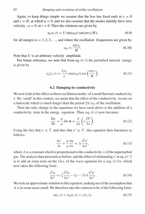
92 Damping and excitation of stellar oscillations
Again, to keep things simple we assume that the box has fixed ends at x = 0and x = H , at which u = 0, and we also assume that the modes initially have zerovelocity , u = 0, at t = 0. Then the solutions are given by
un(x, t) = U sin(ωnt) sin(nπx/H ), (6.9)
for all integers n = 1, 2, 3, . . ., and where the oscillation frequencies are given by
ωn = nπcs
H. (6.10)
Note that U is an arbitrary velocity amplitude.For future reference, we note that from eq. (6.5) the perturbed internal energy
is given by
e′n(x, t) = Ucs
γcos(ωnt) cos
(nπx
H
). (6.11)
6.2 Damping by conductivity
We now look at the effect on these oscillation modes of a small thermal conductivityλ. By ‘small’ in this context, we mean that the effect of the conductivity occurs ona timescale which is much longer than the period 2π/ωn of the oscillation.
Then the only change to the equations we have used above is the addition of aconductivity term in the energy equation. Thus, eq. (6.4) now becomes
De
Dt+ p
ρdiv u = ∂
∂x
(λ∂T
∂x
). (6.12)
Using the fact that e ∝ T , and thus that e′ ∝ T ′, this equation then linearizes asfollows:
∂e′
∂t+ p
ρ
∂u
∂x= �
∂2e′
∂x2, (6.13)
where � is a constant which is proportional to the conductivity λ of the unperturbedgas. The analysis then proceeds as before, and the effect of eliminating e′ in eq. (6.7)is to add an extra term on the r.h.s. of the wave equation for u (eq. (6.8)), whichnow takes the following form:
∂2u
∂t2= c2
s∂2u
∂x2− (γ − 1)�
∂3e′
∂x3. (6.14)
We seek an approximate solution to this equation, making use of the assumption that� is in some sense small. We therefore take the solution to be of the following form:
u(x, t) = un(x, t) + y(x, t), (6.15)
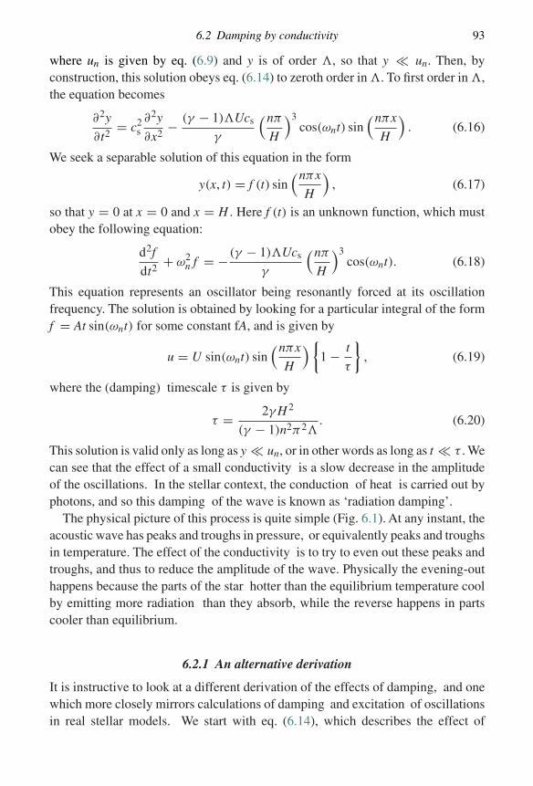
6.2 Damping by conductivity 93
where un is given by eq. (6.9) and y is of order �, so that y � un. Then, byconstruction, this solution obeys eq. (6.14) to zeroth order in �. To first order in �,the equation becomes
∂2y
∂t2= c2
s∂2y
∂x2− (γ − 1)�Ucs
γ
(nπ
H
)3cos(ωnt) sin
(nπx
H
). (6.16)
We seek a separable solution of this equation in the form
y(x, t) = f (t) sin(nπx
H
), (6.17)
so that y = 0 at x = 0 and x = H . Here f (t) is an unknown function, which mustobey the following equation:
d2f
dt2+ ω2
n f = −(γ − 1)�Ucs
γ
(nπ
H
)3cos(ωnt). (6.18)
This equation represents an oscillator being resonantly forced at its oscillationfrequency. The solution is obtained by looking for a particular integral of the formf = At sin(ωnt) for some constant fA, and is given by
u = U sin(ωnt) sin(nπx
H
){1 − t
τ
}, (6.19)
where the (damping) timescale τ is given by
τ = 2γ H 2
(γ − 1)n2π2�. (6.20)
This solution is valid only as long as y � un, or in other words as long as t � τ . Wecan see that the effect of a small conductivity is a slow decrease in the amplitudeof the oscillations. In the stellar context, the conduction of heat is carried out byphotons, and so this damping of the wave is known as ‘radiation damping’.
The physical picture of this process is quite simple (Fig. 6.1). At any instant, theacoustic wave has peaks and troughs in pressure, or equivalently peaks and troughsin temperature. The effect of the conductivity is to try to even out these peaks andtroughs, and thus to reduce the amplitude of the wave. Physically the evening-outhappens because the parts of the star hotter than the equilibrium temperature coolby emitting more radiation than they absorb, while the reverse happens in partscooler than equilibrium.
6.2.1 An alternative derivation
It is instructive to look at a different derivation of the effects of damping, and onewhich more closely mirrors calculations of damping and excitation of oscillationsin real stellar models. We start with eq. (6.14), which describes the effect of
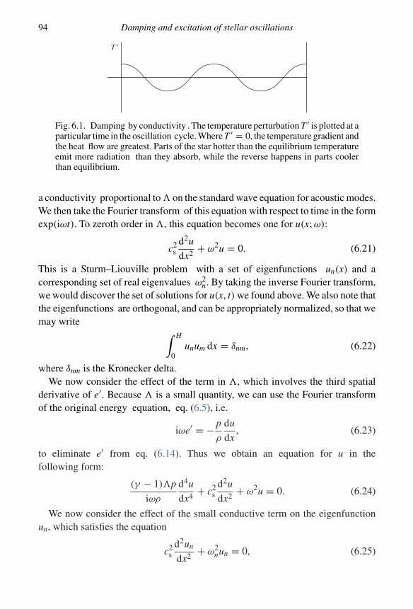
94 Damping and excitation of stellar oscillations
T �
Fig. 6.1. Damping by conductivity . The temperature perturbation T ′ is plotted at aparticular time in the oscillation cycle. Where T ′ = 0, the temperature gradient andthe heat flow are greatest. Parts of the star hotter than the equilibrium temperatureemit more radiation than they absorb, while the reverse happens in parts coolerthan equilibrium.
a conductivity proportional to � on the standard wave equation for acoustic modes.We then take the Fourier transform of this equation with respect to time in the formexp(iωt). To zeroth order in �, this equation becomes one for u(x; ω):
c2s
d2u
dx2+ ω2u = 0. (6.21)
This is a Sturm–Liouville problem with a set of eigenfunctions un(x) and acorresponding set of real eigenvalues ω2
n. By taking the inverse Fourier transform,we would discover the set of solutions for u(x, t) we found above. We also note thatthe eigenfunctions are orthogonal, and can be appropriately normalized, so that wemay write ∫ H
0unum dx = δnm, (6.22)
where δnm is the Kronecker delta.We now consider the effect of the term in �, which involves the third spatial
derivative of e′. Because � is a small quantity, we can use the Fourier transformof the original energy equation, eq. (6.5), i.e.
iωe′ = − p
ρ
du
dx, (6.23)
to eliminate e′ from eq. (6.14). Thus we obtain an equation for u in thefollowing form:
(γ − 1)�p
iωρ
d4u
dx4+ c2
sd2u
dx2+ ω2u = 0. (6.24)
We now consider the effect of the small conductive term on the eigenfunctionun, which satisfies the equation
c2s
d2un
dx2+ ω2
nun = 0, (6.25)
6.3 The effect of heating and cooling – the ε-mechanism 95
with eigenfrequency ωn. To do this we assume as before that the solution to theperturbed equation is of the form u = un + y, with y � un. But now we can use thefact that the eigenfunctions of a Sturm–Liouville problem form a complete set, sothat any function y can be written as an appropriate sum over them. Thus we take
u = un +∑m�=n
amum, (6.26)
where the coefficients am are of order � and are to be determined. In fact for ourpresent purposes we are not interested in finding these, but are, rather, interestedin calculating the perturbation to the eigenfrequency ωn. We therefore substituteeq. (6.26) into eq. (6.24), keeping only terms that are first order in �, to yield
(ω2n − ω2)un +
∑m�=n
{(ω2m − ω2)amum} = 1
iω
(γ − 1)�p
ρ
d4un
dx4. (6.27)
We now multiply both sides of this equation by un, integrate from zero to H anduse the orthogonal property of the eigenfunctions to give an equation for the neweigenfrequency ω:
ω2n − ω2 = 1
iω
(γ − 1)�p
ρ
∫ H
0un
d4un
dx4dx. (6.28)
Since we expect the new eigenfrequency to be close to the original one, we let
ω = ωn + iε, (6.29)
where ε � ωn. Then, to first order in ε, we find
ε = (γ − 1)�p
2ω2nρ
∫ H
0
(d2un
dx2
)2
dx, (6.30)
where we have integrated by parts twice. This demonstrates that ε > 0. Thus thequantities which formerly oscillated in the form exp(iωnt) now vary with time asexp(iωt) = exp(iωnt − εt). These correspond to oscillations which are damped(since ε > 0), with a damping timescale of τ = 1/ε. This solution is now validfor all time t > 0 and not just for 0 < t � τ .
6.3 The effect of heating and cooling – the ε-mechanism
For most of their lives, stars radiate because of the release of nuclear energy in theirinteriors. For a low-mass main-sequence star like the Sun, the energy productionprocess involves the conversion of hydrogen to helium in a set of reactions calledthe p-p chain, since the first reaction in the process requires the fusion of two protons
96 Damping and excitation of stellar oscillations
(or hydrogen nuclei). The energy production rate of this process has the followingrough dependence:
εnuc(ρ, T ) ∝ ρTα , (6.31)
where εnuc is the rate of energy release per unit mass and the index α ∼ 3–5. Inmore massive stars on the main sequence the fusion of hydrogen to helium proceedsby a catalytic reaction cycle involving carbon, nitrogen and oxygen nuclei, calledthe CNO cycle. The energy production rate for this process can be written as above,but now with α ∼ 16 − 18. Later in their lives, stars survive by fusing helium nucleito form carbon. Since it takes three helium nuclei to form a carbon nucleus, this isessentially a three-body process, and so has a stronger dependence on the density. Itis also very sensitive to temperature and can typically be written as something like
εnuc(ρ, T ) ∝ ρ2T 40. (6.32)
Energy generation like this means that the energy equation has a source term,so that
De
Dt+ p
ρdiv u = H(ρ, e), (6.33)
where H = ρεnuc is the energy generation rate per unit volume and we have usedthe fact that for a perfect gas T ∝ e. In linearized form this equation becomes
∂e′
∂t+ p
ρ
∂u
∂x= e′ ∂H
∂e
∣∣∣∣ρ
+ ρ′ ∂H∂ρ
∣∣∣∣e. (6.34)
Proceeding with the analysis as before, the wave equation for u now has some extraterms and becomes
∂2u
∂t2= c2
s∂2u
∂x2−(
1
e
∂H∂e
)∂e′
∂x−(
1
e
∂H∂ρ
)∂ρ′
∂x. (6.35)
We saw above that the nuclear energy generation rate in stars typically dependsmuch more strongly on T than on ρ. Thus,
∂H∂ ln e
� ∂H∂ ln ρ
. (6.36)
This implies that we can, as a first approximation, neglect the ρ′ term in thisequation. This also has the beneficial effect of simplifying the algebra. Includingthis term adds little of interest and serves mainly to complicate the analysis. So weuse the equation in the following form:
∂2u
∂t2= c2
s∂2u
∂x2− 1
e2
∂H∂ ln e
∂e′
∂x. (6.37)
To study stability we again assume that the heating term has only a small effectover an individual oscillation cycle, so that we can treat this term as small. Thus we
6.4 The effect of opacity – the κ-mechanism 97
start again with a particular oscillation mode which would be present in the absenceof the heating term. As before we choose
un(x, t) = U sin(ωnt) sin(nπx/H ), (6.38)
for which
∂e′
∂x= −Ucs
γ
nπ
Hcos(ωnt) sin(nπx/H ). (6.39)
Then we assume that adding the small heating term leads, in a first approximation,to a solution of the following form:
u(x, t) = un(x, t) + y(x, t), (6.40)
where y � un. In this case the equation for y is given by
∂2y
∂t2= c2
s∂2y
∂x2+ 1
e2
∂H∂ ln e
Ucs
γ
nπ
Hcos(ωnt) sin
(nπx
H
). (6.41)
This is very similar to eq. (6.16), we had before, and by essentially the same analysiswe deduce that the oscillations grow in amplitude if ∂H/∂ ln e > 0. This makesphysical sense. During the oscillation cycle, when the gas is most compressed,it is also hottest. If ∂H/∂ ln e > 0, the energy production mechanism adds yetmore heat to the gas at this stage and the oscillation grows. This is known asoverstability.
This effect is no longer thought to be the driving mechanism for most stellarpulsations. What happens instead is that either the damping effects of conductivityoverwhelm this type of excitation, or the temperature sensitivity drives the nuclearburning regions of the star convective. On a historical note, the possibility of thismechanism led Sir James Jeans (1929) to the conclusion that nuclear fusion wasunlikely to be the process which powers stars.
6.4 The effect of opacity – the κ-mechanism
The mechanism which is now thought to drive most observed large-scale stellaroscillations is one which taps the outward heat flux. It is caused by the temperaturesensitivity of the thermal conductivity (or, in stellar parlance, the opacity κ).To investigate this mechanism we need an equilibrium state with a temperaturegradient and a non-zero heat flux down this gradient. For this reason we use as ourillustrative base state the polytropic atmosphere, whose oscillation properties wediscussed in Chapter 4.
There we used the coordinate x to measure distance from the top of the atmosphereat x = 0, and we assumed a solid base at x = H . The pressure and density wererelated by p ∝ ρ1+1/m, and we found ρ ∝ xm, p ∝ xm+1 and T ∝ e ∝ x.
98 Damping and excitation of stellar oscillations
Perturbing this atmosphere, assuming purely vertical motions, the linearizedmass conservation equation is given by
∂ρ′
∂t+ u
∂ρ
∂x+ ρ
∂u
∂x= 0 (6.42)
and the linearized equation of motion is given by
ρ∂u
∂t= −∂p′
∂x+ ρ′g, (6.43)
where the gravity g > 0 is fixed and given by hydrostatic equilibrium:
g = 1
ρ
dp
dx. (6.44)
We assume that the atmosphere is a perfect gas, so that p = (γ − 1)ρe, and theperturbed equation of state yields
p′
p= ρ′
ρ+ e′
e. (6.45)
Using the mass conservation equation to substitute for div u, the thermalequation, eq. (6.12), becomes
ρDe
Dt= p
ρ
Dρ
Dt+ ρdiv(λ∇T ). (6.46)
Using the equation of state, this can then be written as follows:
Dρ
Dt= 1
c2s
Dp
Dt− ρ
γ ediv(λ∇T ). (6.47)
In the equilibrium situation, this equation implies that
λdT
dx= const. (6.48)
Since dT/dx = constant, this implies a form for the dependence of the conductivityλ on density and temperature such that it is constant through the atmosphere. Sinceρ ∝ T m, we can write this dependence as λ(ρ, T ) = F(ρ/T m) for some arbitraryfunction F . (Note that this is in general not true for the real physical conductivity ,but is forced on us by our simplifying assumption that the atmosphere is polytropic.This does not affect the essential physics of our treatment of the κ-mechanism.)
To keep the algebra simple, we now further assume that the unperturbedatmosphere is neutrally stable (or marginally unstable) to convection, i.e. γ =1 + 1/m. This means that A = 0, or equivalently that
∇ρ = 1
c2s∇p. (6.49)
6.4 The effect of opacity – the κ-mechanism 99
In this case the linearized version of the thermal equation, eq. (6.46), becomes
∂ρ′
∂t= 1
c2s
∂p′
∂t− Q′, (6.50)
where Q′ is the Eulerian perturbation of the quantity Q representing the heat flux:
Q = ρ
γ ediv(λ∇T ). (6.51)
6.4.1 The underlying oscillations: Q′ = 0
We start by considering the oscillations which occur when there is no perturbationto the heat flux, i.e. Q′ = 0. In fact, we worked out the detailed properties of theoscillations in this case in Chapter 4. Here we do not need the details, but need toderive some of their properties, making use of the fact that this is a Sturm–Liouvilleproblem.
When Q′ = 0 and the atmosphere is convectively neutral, the thermal equationis simply given by
p′ = c2s ρ
′. (6.52)
Using this, eqs. (6.42) and (6.43) can be combined to yield
∂2u
∂t2= ∂
∂x
{c2
s
ρ
∂
∂x(ρu)
}. (6.53)
We now Fourier analyse in time in the form u ∝ exp(iωt) and obtain the eigenvalueequation describing the oscillation modes as follows:
d
dx
{c2
s
ρ
d
dx(ρun)
}+ ω2
nun = 0. (6.54)
The oscillation modes are orthogonal, and can be normalized, so that∫ H
0ρumun dx = δmn (6.55)
(see Problem 5.4.1).
6.4.2 Perturbing the underlying oscillations: Q′ �= 0
We now allow the heat flux to vary so that Q′ �= 0. At the same time we assume thatthe effect of this term is small in the sense that it takes many oscillation periods tohave an effect. Thus it will produce small perturbations in the oscillation frequencyωn and in the eigenfunction un(x).
100 Damping and excitation of stellar oscillations
With this extra term, eq. (6.53) becomes
∂2u
∂t2= ∂
∂x
{c2
s
ρ
∂
∂x(ρu)
}+ 1
ρ
∂
∂x[c2
s Q′]. (6.56)
We now consider the perturbation to the mode u0 = un(x) sin(ωnt) in thefollowing form:
u(x, t) = un(x) sin(ωnt) + y(x, t), (6.57)
where y is small. Substituting this in eq. (6.56), and using the fact that un satisfieseq. (6.53), we find that y satisfies the following equation:
∂2y
∂t2− ∂
∂x
[c2
s
ρ
∂
∂x(ρy)
]= G(x) sin(ωnt). (6.58)
Here G(x) is some function of x which comes from substituting the solution un(x),and the corresponding density ρn(x) and temperature Tn(x), into the term Q′.
As before we look for a solution of the form y = un(x)f (t), which yields[d2f
dt2− ω2
n f
]un(x) = G(x) sin(ωnt). (6.59)
We now use the orthogonality properties of the eigenfunctions. We multiply thisequation by ρun and integrate from 0 to H . This gives an equation for the functionf (t) as follows:
d2f
dt2− ω2
n f =[∫ H
0ρun(x)G(x) dx
]sin(ωnt). (6.60)
This is a resonantly forced harmonic oscillator, and, as we found before, whetheror not the oscillations grow or damp depends on the sign of the term in squarebrackets. This sign depends on the functional form of the dependence of the thermalconductivity λ on the density ρ and temperature T . Thus if we choose a form of λ
which makes the square bracket positive, the perturbations will grow and the staroscillates.
The physics of the instability for this choice of λ is not easy to see in simpleterms. What happens in essence is that the temperature and density dependenceof the conductivity manipulate the heat flux through the atmosphere in such away that there is a net heat gain by the oscillating gas when it is compressed(higher density and so higher temperature), raising its temperature still further.In a real star the temperature sensitivity of the stellar opacity needed to makethis mechanism work occurs at the point where hydrogen changes from beingpredominantly neutral (low opacity) to predominantly ionized (high opacity). Thenthe hottest gas experiences a sudden increase in opacity as it gains a little heat, soabsorbing more of the stellar radiation flux and raising the temperature still further.
6.5 Further reading 101
Such hydrogen ionization zones require temperatures ∼ 6000 − 10 000 K. For thiseffect to drive oscillations, there must not be too much mass above the ionizationzone, so the surface (effective) temperature Te must have values of this order also.This explains the position of the main instability strip in the Hertzsprung–Russelldiagram. For stars with little hydrogen there is another instability strip at highereffective temperatures corresponding to helium ionization.
6.5 Further reading
More details on excitation mechanisms for stellar oscillations, as well as thecomputation of excitation and damping timescales, can be found in Unno et al.(1979) and in Cox (1980). On a historical note, readers might be intrigued by thediscussion of Jeans (1929, Chap. IV), who uses a simple stability analysis to try toconstrain possible stellar energy-generation mechanisms.
7
Magnetic instability in a static atmosphere
In Chapter 4 we considered the stability of a static fluid configuration againstconvective instabilities, or buoyancy. We found that for stability the specific entropymust increase upwards. In this chapter we again consider the stability of a staticatmosphere, but with the complication of an added magnetic field. We shall find thatthe magnetic field can act either to stabilize or to de-stabilize the fluid. It is possibleto derive a variational principle for perturbations of a fluid containing a magneticfield, just as we did for a non-magnetic fluid in Chapter 4 (see Problem 4.7.4).Of course, the expressions we would derive in doing so contain all the informationrequired to decide stability. But we found in Chapter 4 that we had to manipulatecarefully the expressions we derived in the variational principle to extract a usefulstability criterion – the Schwarzschild criterion. Adding a magnetic field makes theexpressions in the variational principle much more complex, simply because thegeometry of the magnetic field and its interaction with the fluid add more degrees offreedom, and there is no simple stability criterion. Accordingly we adopt a simpler,less comprehensive, approach here.
There are some guiding concepts with which a theoretical astrophysicist shouldbe familiar, and we illustrate these here. We discuss the two distinct, but oftenconfused, modes of instability – the buoyancy instability and the Parker instability.As before we keep try to keep the situation simple, in order to bring out the physicsof the situation without obscuring it in mathematical detail. Even so, the inclusionof a magnetic field to the perturbation equations does considerably increase thedegree of mathematical complexity.
7.1 Magnetic buoyancy
We consider an atmosphere with uniform gravity g = (0, 0, −g) in Cartesiancoordinates and with a horizontal magnetic field B = (0, B(z), 0). The equation
102
7.1 Magnetic buoyancy 103
of hydrostatic equilibrium is simply given by
d
dz
(p + 1
2B2)
= −ρg. (7.1)
We consider an equilibrium magnetic field which is zero in the upper half-space,i.e. B = 0 for z > 0, and uniform in the lower half-space, B = (0, B0, 0) for z < 0,where B0 is a constant. Thus the field has a sharp boundary at z = 0, and there is asheet current of the form j = (Jδ(z), 0, 0) flowing in the z = 0 plane.
Integrating eq. (7.1) across the z = 0 plane, we see that the total pressure P (gasplus magnetic, i.e. P = p + B2
0/2) must be continuous across z = 0. Thus if the gaspressure just below z = 0, i.e. at z = 0−, is p = p0, the gas pressure just above, atz = 0+, must be p = p0 + �p, where �p = B2
0/2. We assume that the gas obeysthe perfect gas law, p = (R/µ)ρT . We must also require that the temperature Tis continuous at z = 0, for otherwise there would be an infinite heat flux at thatpoint, however small the conductivity . We conclude from all this that there mustbe a jump in the density at z = 0. If the density at z = 0− is ρ = ρ0 and the densityat z = 0+ is ρ = ρ1, then
Rρ1T
µ= Rρ0T
µ+ 1
2B2. (7.2)
Alternatively we may write ρ1 = ρ0 + �ρ, where
�ρ
ρ0= V 2
A /2
RT/µ. (7.3)
Here, VA is the Alfvén speed in z < 0, where V 2A = B2
0/ρ0.Thus equilibrium requires that we have a heavy fluid above a light one in a
gravitational field. This happens because the magnetic field provides pressure,but no mass. It seems likely that this situation is unstable, and, as we now show,this is indeed the case. To simplify the analysis still further, we consider instabilityover a region very close to the plane z = 0, in particular a region which is muchsmaller than the atmospheric scaleheight H ∼ p0/gρ0. This means that we canassume the unperturbed pressures and densities to be uniform. Moreover we shallconsider only perturbations for which the perturbed velocity obeys div u = 0. Thisis a useful device which implies that Lagrangian density perturbations vanish,δρ = 0, and so cuts out the possibility of acoustic waves. Since we expect anyinstability in this situation to be caused by gravity (g-modes) rather than by soundwaves (p-modes), this has the effect of simplifying the analysis without excludingany of the essential physics.
We consider a perturbation to the magnetic field of the form B = B0 + b, whereb = (bx, by, bz) is small, and a small resulting velocity of the form u = (u, v, w).
104 Magnetic instability in a static atmosphere
The linearized induction equation is then given by
∂b∂t
= curl(u ∧ B0). (7.4)
Expanding this expression and using the imposed condition div u = 0, we obtain
∂b∂t
= B0∂u∂y
. (7.5)
The linearized form of the momentum equation, including the magnetic terms,is given by
ρ∂u∂t
= −∇p′ − B0 ∧ (curl b). (7.6)
In terms of components, this expands to yield
ρ∂u
∂t= −∂p′
∂x+ B0
[∂bx
∂y− ∂by
∂x
], (7.7)
ρ∂v
∂t= −∂p′
∂y(7.8)
and
ρ∂w
∂t= −∂p′
∂z+ B0
[∂bz
∂y− ∂by
∂z
]. (7.9)
We note first that by taking the curl of eq. (7.6), and using eq. (7.5), we obtainan equation for the vorticity, ω = ∇ ∧ u, of the perturbed velocity field:
∂2ω
∂t2= V 2
A∂2ω
∂y2. (7.10)
This implies that a perturbation which has vorticity is propagated away along thefield lines as an Alfvén wave in the y-direction. Such perturbations therefore donot lead to instability. Thus we need only consider perturbations which have zerovorticity, for which curl u = 0. For such perturbations we may write
u = −∇�, (7.11)
where � is the velocity potential, and, since div u = 0, we also have that � obeysLaplace’s equation:
∇2� = 0. (7.12)
We now take Fourier transforms so that all perturbed quantities vary as∝ exp {iωt + ik · r}. To ensure that �, and therefore the other quantities, obeyLaplace’s equation, we need to place a constraint on the components of k.
7.1 Magnetic buoyancy 105
In the lower half-space z < 0, we need to write
� = �0 exp {iωt + ikxx + ikyy + (k2x + k2
y )1/2z}, (7.13)
where �0 is a constant, the magnitude of kz = k⊥ = (k2x +k2
y )1/2 is chosen such thatLaplace’s equation is satisfied, and its sign is chosen to ensure that the perturbationvanishes at large distances, i.e. � → 0 as z → −∞.
Similarly in the upper half-space z > 0, we need to write
� = �1 exp {iωt + ikxx + ikyy − (k2x + k2
y )1/2z}, (7.14)
where �1 is a constant, the magnitude of kz = k⊥ is chosen such that Laplace’sequation is satisfied, and its sign is chosen to ensure that the perturbation vanishesat large distances, i.e. � → 0 as z → +∞.
There are two boundary conditions which we must apply at z = 0. First wemust ensure that the vertical velocity is continuous across the boundary. Otherwisethe two fluid regions would come apart! The vertical component of the velocity isgiven by w = ∂�/∂z. Evaluating these in the upper and lower half-planes, andequating them at z = 0, we obtain
�0 = −�1. (7.15)
Second, by integrating eq. (7.9) across the boundary,∫ ε
−εdz, and then letting
ε → 0, we find that the perturbation to the total pressure P = p + B2/2 (gas plusmagnetic) given by
P′ = p′ + B0by (7.16)
must be continuous across the boundary.We note that the boundary in the perturbed fluid is at
z = ζ exp {iωt + ikxx + ikyy}, (7.17)
where ζ is the z-component of the Lagrangian displacement and is related to thevertical velocity perturbation by w = iωζ . Thus, just above the boundary at z = 0+we have
iωζ = +k⊥�1, (7.18)
and just below the boundary at z = 0− we have
iωζ = −k⊥�0. (7.19)
Since the boundary is no longer at z = 0 we must apply the condition that it is theLagrangian perturbation of the total pressure, δP = P′ + ξ · ∇P = P′ − ζρg,which is continuous at z = 0. Note that here we have used the equilibrium condition∇P = (0, 0, −gρ). Thus to apply the second boundary condition we have that
p′1 − ζρ1g = p′
0 + B0by − ζρ0g, (7.20)
106 Magnetic instability in a static atmosphere
where both sides are to be evaluated at z = 0. To do so we need expressions for p′1,
p′0 and by. From the y-component of eq. (7.5), using the fact that v = −∂�/∂y, we
have in z < 0 that
iωby = B0k2y �0. (7.21)
From eq. (7.8) we have in z < 0 that
iω�0 = p′0
ρ0(7.22)
and in z > 0 that
iω�1 = p′1
ρ1. (7.23)
Putting all this together, the second boundary condition (eq. (7.20)) becomes
iωρ1�1 − ρ1gk⊥�1
iω= iωρ0�0 + B2
0
k2y �0
iω+ ρ0g
k⊥�0
iω. (7.24)
Tidying this up, and using the first boundary condition (which yielded �0 = −�1),this gives a dispersion relation for the modes:
ω2 = −gk⊥(ρ1 − ρ0) − ρ0V 2A k2
y
ρ0 + ρ1. (7.25)
This fluid configuration is unstable for those modes with ω2 < 0, i.e. for thosemodes with
k2y <
gk⊥V 2
A
�ρ
ρ0. (7.26)
The most unstable modes, i.e. those with the most negative value of ω2, are thosewith ky = 0. These modes have no y-dependence. Since the field is in the y-direction,this implies that the fluid motions are all perpendicular to the field. Thus the fieldlines are not stretched, and so no extra magnetic energy is created. From anenergy point of view these modes can tap gravitational energy by interchangingfluid elements of different density in the gravitational field, without paying a penaltyin magnetic energy by having to stretch field lines.
This instability is simple magnetic buoyancy . It is the analogue of the convectiveinstability and comes about because the magnetic field provides the pressure but nomass. Thus in pressure equilibrium matter containing magnetic field is lighter thanmatter without. As we have seen, it operates even when the fluid is incompressible.
7.2 The Parker instability
The concept of a buoyancy instability driven by magnetic fields contributingpressure but no mass is easily visualized when the fluids (or the perturbations) are
7.2 The Parker instability 107
incompressible. However, most astronomical fluids are not incompressible, and themodes by which buoyancy can drive an instability are different from those derivedabove. We sketch here the analysis of a simple problem given by Parker (1979),which serves to illustrate the physical differences.
We consider again a stratified atmosphere with fixed gravity, g = (0, 0, −g),and horizontal magnetic field, B0 = (0, B0(z), 0), lying in the y-direction. Thus,although div B0 = 0, we have curl B0 �= 0, and there is a current proportionalto −∂B0/∂z in the x-direction. We take the equation of state of the unperturbedatmosphere to be isothermal, so that density and pressure are related by p = c2
isρ,where cis is the isothermal sound speed. For simplicity we assume that the magneticfield is such that the magnetic pressure is a constant fraction α of the gas pressure,i.e. B2
0/2 = αp. Then the equilibrium equation (eq. (7.1)) yields the followingsolutions:
p(z) = p0 exp(−z/H ), (7.27)
ρ(z) = ρ0 exp(−z/H ) (7.28)
and
B0(z) = B00 exp(−z/2H ), (7.29)
where the scaleheight H is given by
H = (1 + α)c2is
g. (7.30)
Here p0, ρ0 and B00 are all constants, being values of the quantities at the referencelevel z = 0.
We now write down the linearized perturbation equations. The equation of massconservation is given by
∂ρ′
∂t+ w
dρ
dz= −ρ div u. (7.31)
We assume that the perturbations are adiabatic, so that δp = (γ p/ρ)δρ. Sincethe basic atmosphere is isothermal, this means, according to the Schwarzschildcriterion, that, in the absence of a magnetic field, it is stable to convection. Themass conservation equation becomes
∂p′
∂t= γ c2
is∂ρ′
∂t− (γ − 1)c2
isρw
H. (7.32)
The linearized induction equation,
∂b∂t
= curl(u ∧ B0), (7.33)
108 Magnetic instability in a static atmosphere
has three components:
∂bx
∂t= B0
∂u
∂y, (7.34)
∂by
∂t= −B0
∂u
∂x− B0
∂w
∂z+ B0
w
2H(7.35)
and∂bz
∂t= B0
∂w
∂y. (7.36)
In the linearized momentum equation we need to recall that curl B0 �= 0, so it isgiven by
ρ∂u∂t
= −∇p′ − B0 ∧ (curl b) − b ∧ (curl B0) + ρ′g. (7.37)
This has the following three components:
ρ∂u
∂t= −∂p′
∂x+ B0
{∂bx
∂y− ∂by
∂x
}, (7.38)
ρ∂v
∂t= −∂p′
∂y− B0
{bz
2H
}(7.39)
and
ρ∂w
∂t= −∂p′
∂z+ B0
{∂bz
∂y− ∂by
∂z+ by
2H
}− gρ′. (7.40)
In total we now have eight partial differential equations for the eight variablesb, u, p′ and ρ′. If the unperturbed atmosphere were uniform, the obvious thing todo next would be to Fourier transform with all variables ∝ exp(iωt + ik · r). Wewould then be left with eight linear, homogeneous, algebraic equations, leaving an8 × 8 determinant to be evaluated to give us the dispersion relation. Parker’s trickwas to realize that something similar can be achieved by making the followingassumptions about the behaviour of the variables. We take
p′ ∝ exp(iωt + ik · r) × exp(−z/2H ), (7.41)
ρ′ ∝ exp(iωt + ik · r) × exp(−z/2H ), (7.42)
u ∝ exp(iωt + ik · r) × exp(+z/2H ) (7.43)
and
b ∝ exp(iωt + ik · r). (7.44)
These relationships imply that both the magnetic energy perturbation, b2, andthe kinetic energy perturbation, ρu2, are independent of z. By making these
7.2 The Parker instability 109
substitutions we then find that the resulting algebraic equations are linearand homogeneous. Importantly the exponential z-dependence of the quantitiesdescribing the unperturbed atmosphere cancels out. We are then left with an8 × 8 determinant to evaluate in order to obtain the dispersion relation. Thisnecessitates a large amount of messy, but straightforward, algebra, which we leaveto the reader’s imagination and omit. To make the algebra simpler, the resultingdispersion relation is given by Parker (1979) in terms of dimensionless quantities.We define a dimensionless frequency � in terms of the time for an isothermal waveto cross a scaleheight,
� = ωH
cis, (7.45)
and a dimensionless wavevector, in terms of the scaleheight,
q = Hk. (7.46)
With these the full dispersion relation is given by
�4−�2(2α + γ )[q2y + q2
z +1/4] + q2y{2αγ (q2
y + q2z +1/4)−(1+ α)(1+ α−γ )}
+ q2x
2α(q2x + q2
y)−�2[γ�4− �2{2αγ q2
y − 2α(2α + γ )q2z + (γ −1)+(1/2)αγ }
− 4α2γ q2y(q
2z + 1/4)] = 0. (7.47)
This is a sixth-order equation for �, or because of time-symmetry a cubicequation for �2. On physical grounds, we expect the roots to come in pairs, withone pair representing (magnetically modified) acoustic waves, one representing(magnetically modified) buoyancy waves and one representing magnetic (torsionalor Alfvén) waves. In the previous section we were able to simplify the analysis byremoving the acoustic waves by setting div u = 0 and the magnetic waves bytaking curl u = 0. Here we do not have that luxury. Nevertheless, we still expectany instability to come through buoyancy waves. However, we have already seenthat in the absence of a field the unperturbed atmosphere is buoyantly stable.
We do not attempt a general analysis of the dispersion relation, but rather considertwo simple types of modes.
7.2.1 Modes with ky = 0
Since the unperturbed magnetic field lies in the y-direction, if we set ky = 0, orequivalently qy = 0 or ∂/∂y = 0, the fluid motions are perpendicular to the fieldand so do not stretch the field lines. In the incompressible case, these were the mostunstable modes, because such fluid motions did not change the magnetic energy.The dispersion relation now becomes
�2[�4 − �2(2α + γ )(q2x + q2
z + 1/4) + q2x(α(α + γ ) + γ − 1)] = 0. (7.48)
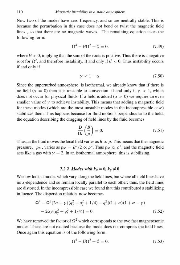
110 Magnetic instability in a static atmosphere
Now two of the modes have zero frequency, and so are neutrally stable. This isbecause the perturbation in this case does not bend or twist the magnetic fieldlines , so that there are no magnetic waves. The remaining equation takes thefollowing form:
�4 − B�2 + C = 0, (7.49)
where B > 0, implying that the sum of the roots is positive. Thus there is a negativeroot for �2, and therefore instability, if and only if C < 0. Thus instability occursif and only if
γ < 1 − α. (7.50)
Since the unperturbed atmosphere is isothermal, we already know that if there isno field (α = 0) then it is unstable to convection if and only if γ < 1, whichdoes not occur for physical fluids. If a field is added (α > 0) we require an evensmaller value of γ to achieve instability. This means that adding a magnetic fieldfor these modes (which are the most unstable modes in the incompressible case)stabilizes them. This happens because for fluid motions perpendicular to the field,the equation describing the dragging of field lines by the fluid becomes
D
Dt
(B
ρ
)= 0. (7.51)
Thus, as the fluid moves the local field varies as B ∝ ρ. This means that the magneticpressure, pM, varies as pM = B2/2 ∝ ρ2. Thus pM ∝ ρ2, and the magnetic fieldacts like a gas with γ = 2. In an isothermal atmosphere this is stabilizing.
7.2.2 Modes with kx = 0, ky �= 0
We now look at modes which vary along the field lines, but where all field lines haveno x-dependence and so remain locally parallel to each other; thus, the field linesare distorted. In the incompressible case we found that this contributed a stabilizinginfluence. The dispersion relation now becomes
�4 − �2(2α + γ )(q2y + q2
z + 1/4) − q2y{(1 + α)(1 + α − γ )
− 2αγ (q2y + q2
z + 1/4)} = 0. (7.52)
We have removed the factor of �2 which corresponds to the two fast magnetosonicmodes. These are not excited because the mode does not compress the field lines.Once again this equation is of the following form:
�4 − B�2 + C = 0, (7.53)
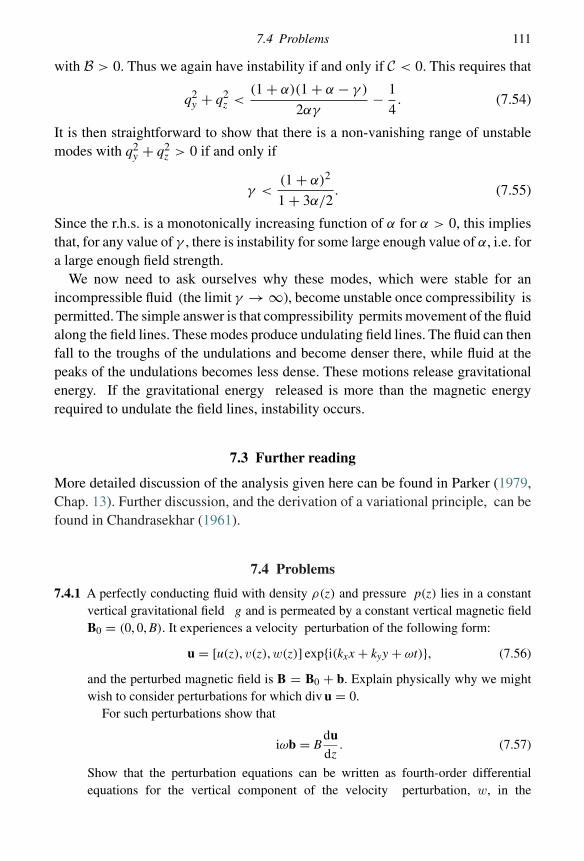
7.4 Problems 111
with B > 0. Thus we again have instability if and only if C < 0. This requires that
q2y + q2
z <(1 + α)(1 + α − γ )
2αγ− 1
4. (7.54)
It is then straightforward to show that there is a non-vanishing range of unstablemodes with q2
y + q2z > 0 if and only if
γ <(1 + α)2
1 + 3α/2. (7.55)
Since the r.h.s. is a monotonically increasing function of α for α > 0, this impliesthat, for any value of γ , there is instability for some large enough value of α, i.e. fora large enough field strength.
We now need to ask ourselves why these modes, which were stable for anincompressible fluid (the limit γ → ∞), become unstable once compressibility ispermitted. The simple answer is that compressibility permits movement of the fluidalong the field lines. These modes produce undulating field lines. The fluid can thenfall to the troughs of the undulations and become denser there, while fluid at thepeaks of the undulations becomes less dense. These motions release gravitationalenergy. If the gravitational energy released is more than the magnetic energyrequired to undulate the field lines, instability occurs.
7.3 Further reading
More detailed discussion of the analysis given here can be found in Parker (1979,Chap. 13). Further discussion, and the derivation of a variational principle, can befound in Chandrasekhar (1961).
7.4 Problems
7.4.1 A perfectly conducting fluid with density ρ(z) and pressure p(z) lies in a constantvertical gravitational field g and is permeated by a constant vertical magnetic fieldB0 = (0, 0, B). It experiences a velocity perturbation of the following form:
u = [u(z), v(z), w(z)] exp{i(kxx + kyy + ωt)}, (7.56)
and the perturbed magnetic field is B = B0 + b. Explain physically why we mightwish to consider perturbations for which div u = 0.
For such perturbations show that
iωb = Bdudz
. (7.57)
Show that the perturbation equations can be written as fourth-order differentialequations for the vertical component of the velocity perturbation, w, in the
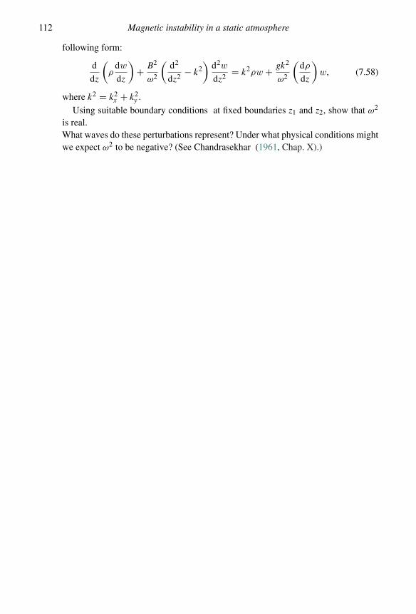
112 Magnetic instability in a static atmosphere
following form:
d
dz
(ρ
dw
dz
)+ B2
ω2
(d2
dz2− k2
)d2w
dz2= k2ρw + gk2
ω2
(dρ
dz
)w, (7.58)
where k2 = k2x + k2
y .
Using suitable boundary conditions at fixed boundaries z1 and z2, show that ω2
is real.What waves do these perturbations represent? Under what physical conditions mightwe expect ω2 to be negative? (See Chandrasekhar (1961, Chap. X).)
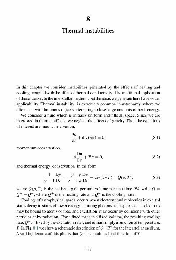
8
Thermal instabilities
In this chapter we consider instabilities generated by the effects of heating andcooling, coupled with the effect of thermal conductivity .The traditional applicationof these ideas is to the interstellar medium, but the ideas we generate here have widerapplicability. Thermal instability is extremely common in astronomy, where weoften deal with luminous objects attempting to lose large amounts of heat energy.
We consider a fluid which is initially uniform and fills all space. Since we areinterested in thermal effects, we neglect the effects of gravity. Then the equationsof interest are mass conservation,
∂ρ
∂t+ div(ρu) = 0, (8.1)
momentum conservation,
ρDuDt
+ ∇p = 0, (8.2)
and thermal energy conservation in the form
1
γ − 1
Dp
Dt− γ
γ − 1
p
ρ
Dρ
Dt= div(λ∇T ) + Q(ρ, T ), (8.3)
where Q(ρ, T ) is the net heat gain per unit volume per unit time. We write Q =Q+ − Q−, where Q+ is the heating rate and Q− is the cooling rate.
Cooling of astrophysical gases occurs when electrons and molecules in excitedstates decay to states of lower energy, emitting photons as they do so. The electronsmay be bound to atoms or free, and excitation may occur by collisions with otherparticles or by radiation. For a fixed mass in a fixed volume, the resulting coolingrate, Q−, is fixed by the excitation rates, and is thus simply a function of temperature,T . In Fig. 8.1 we show a schematic description of Q−(T ) for the interstellar medium.A striking feature of this plot is that Q− is a multi-valued function of T .
113
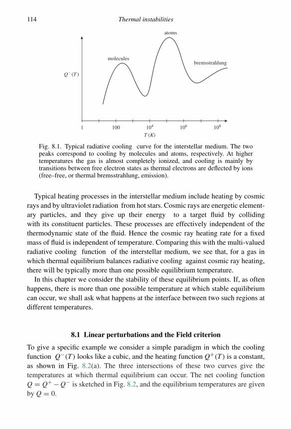
114 Thermal instabilities
Q – (T )
100 104 106
bremsstrahlung
atoms
molecules
T (K)
1 108
Fig. 8.1. Typical radiative cooling curve for the interstellar medium. The twopeaks correspond to cooling by molecules and atoms, respectively. At highertemperatures the gas is almost completely ionized, and cooling is mainly bytransitions between free electron states as thermal electrons are deflected by ions(free–free, or thermal bremsstrahlung, emission).
Typical heating processes in the interstellar medium include heating by cosmicrays and by ultraviolet radiation from hot stars. Cosmic rays are energetic element-ary particles, and they give up their energy to a target fluid by collidingwith its constituent particles. These processes are effectively independent of thethermodynamic state of the fluid. Hence the cosmic ray heating rate for a fixedmass of fluid is independent of temperature. Comparing this with the multi-valuedradiative cooling function of the interstellar medium, we see that, for a gas inwhich thermal equilibrium balances radiative cooling against cosmic ray heating,there will be typically more than one possible equilibrium temperature.
In this chapter we consider the stability of these equilibrium points. If, as oftenhappens, there is more than one possible temperature at which stable equilibriumcan occur, we shall ask what happens at the interface between two such regions atdifferent temperatures.
8.1 Linear perturbations and the Field criterion
To give a specific example we consider a simple paradigm in which the coolingfunction Q−(T ) looks like a cubic, and the heating function Q+(T ) is a constant,as shown in Fig. 8.2(a). The three intersections of these two curves give thetemperatures at which thermal equilibrium can occur. The net cooling functionQ = Q+ − Q− is sketched in Fig. 8.2, and the equilibrium temperatures are givenby Q = 0.
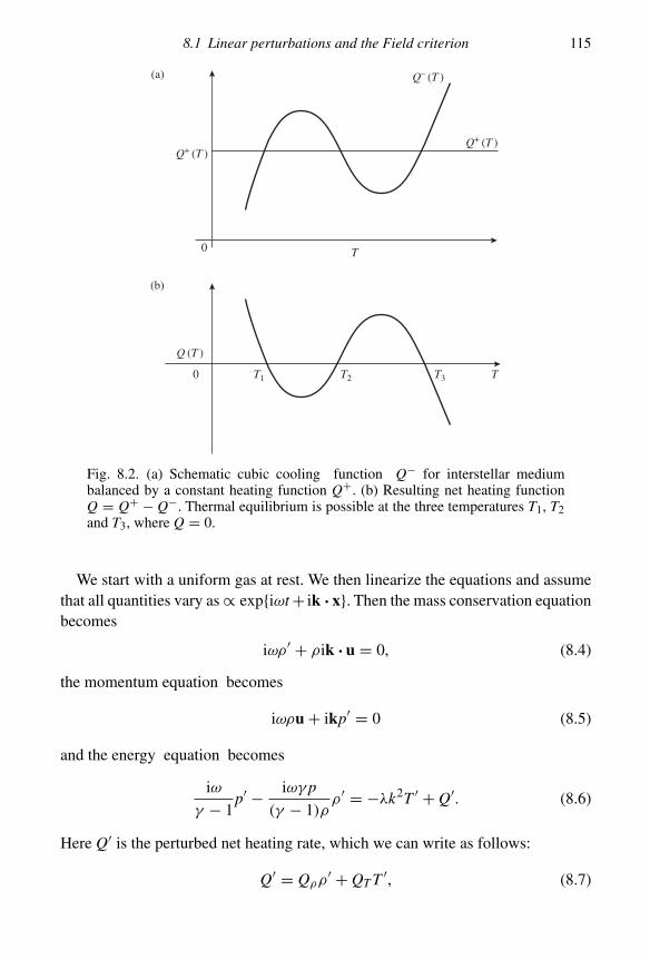
8.1 Linear perturbations and the Field criterion 115
T
Q– (T )
Q+ (T )Q+ (T )
(a)
(b)
0
TT3T2T10
Q (T )
Fig. 8.2. (a) Schematic cubic cooling function Q− for interstellar mediumbalanced by a constant heating function Q+. (b) Resulting net heating functionQ = Q+ − Q−. Thermal equilibrium is possible at the three temperatures T1, T2and T3, where Q = 0.
We start with a uniform gas at rest. We then linearize the equations and assumethat all quantities vary as ∝ exp{iωt + ik · x}. Then the mass conservation equationbecomes
iωρ′ + ρik · u = 0, (8.4)
the momentum equation becomes
iωρu + ikp′ = 0 (8.5)
and the energy equation becomes
iω
γ − 1p′ − iωγ p
(γ − 1)ρρ′ = −λk2T ′ + Q′. (8.6)
Here Q′ is the perturbed net heating rate, which we can write as follows:
Q′ = Qρρ′ + QT T ′, (8.7)
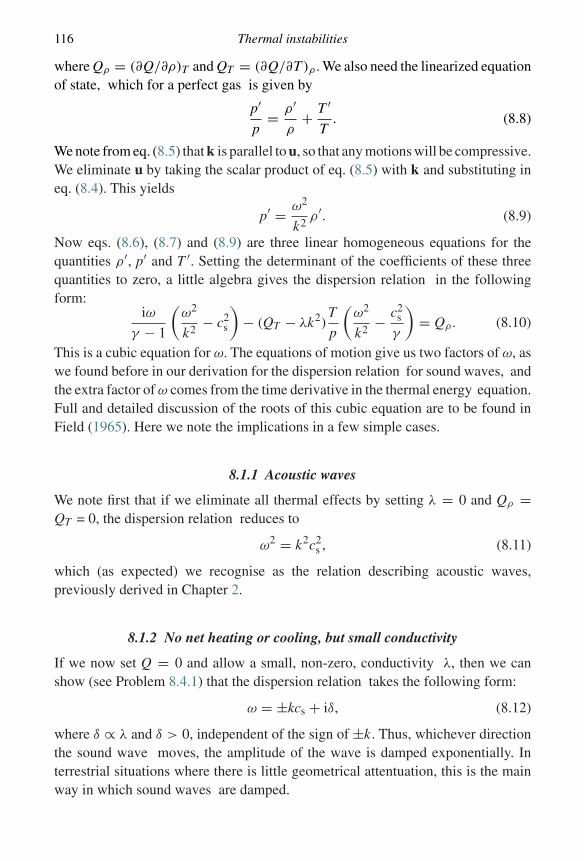
116 Thermal instabilities
where Qρ = (∂Q/∂ρ)T and QT = (∂Q/∂T )ρ . We also need the linearized equationof state, which for a perfect gas is given by
p′
p= ρ′
ρ+ T ′
T. (8.8)
We note from eq. (8.5) that k is parallel to u, so that any motions will be compressive.We eliminate u by taking the scalar product of eq. (8.5) with k and substituting ineq. (8.4). This yields
p′ = ω2
k2ρ′. (8.9)
Now eqs. (8.6), (8.7) and (8.9) are three linear homogeneous equations for thequantities ρ′, p′ and T ′. Setting the determinant of the coefficients of these threequantities to zero, a little algebra gives the dispersion relation in the followingform:
iω
γ − 1
(ω2
k2− c2
s
)− (QT − λk2)
T
p
(ω2
k2− c2
s
γ
)= Qρ . (8.10)
This is a cubic equation for ω. The equations of motion give us two factors of ω, aswe found before in our derivation for the dispersion relation for sound waves, andthe extra factor of ω comes from the time derivative in the thermal energy equation.Full and detailed discussion of the roots of this cubic equation are to be found inField (1965). Here we note the implications in a few simple cases.
8.1.1 Acoustic waves
We note first that if we eliminate all thermal effects by setting λ = 0 and Qρ =QT = 0, the dispersion relation reduces to
ω2 = k2c2s , (8.11)
which (as expected) we recognise as the relation describing acoustic waves,previously derived in Chapter 2.
8.1.2 No net heating or cooling, but small conductivity
If we now set Q = 0 and allow a small, non-zero, conductivity λ, then we canshow (see Problem 8.4.1) that the dispersion relation takes the following form:
ω = ±kcs + iδ, (8.12)
where δ ∝ λ and δ > 0, independent of the sign of ±k. Thus, whichever directionthe sound wave moves, the amplitude of the wave is damped exponentially. Interrestrial situations where there is little geometrical attentuation, this is the mainway in which sound waves are damped.
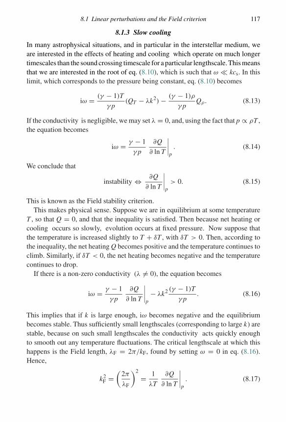
8.1 Linear perturbations and the Field criterion 117
8.1.3 Slow cooling
In many astrophysical situations, and in particular in the interstellar medium, weare interested in the effects of heating and cooling which operate on much longertimescales than the sound crossing timescale for a particular lengthscale. This meansthat we are interested in the root of eq. (8.10), which is such that ω � kcs. In thislimit, which corresponds to the pressure being constant, eq. (8.10) becomes
iω = (γ − 1)T
γ p(QT − λk2) − (γ − 1)ρ
γ pQρ . (8.13)
If the conductivity is negligible, we may set λ = 0, and, using the fact that p ∝ ρT ,the equation becomes
iω = γ − 1
γ p
∂Q
∂ ln T
∣∣∣∣p
. (8.14)
We conclude that
instability ⇔ ∂Q
∂ ln T
∣∣∣∣p
> 0. (8.15)
This is known as the Field stability criterion.This makes physical sense. Suppose we are in equilibrium at some temperature
T , so that Q = 0, and that the inequality is satisfied. Then because net heating orcooling occurs so slowly, evolution occurs at fixed pressure. Now suppose thatthe temperature is increased slightly to T + δT , with δT > 0. Then, according tothe inequality, the net heating Q becomes positive and the temperature continues toclimb. Similarly, if δT < 0, the net heating becomes negative and the temperaturecontinues to drop.
If there is a non-zero conductivity (λ �= 0), the equation becomes
iω = γ − 1
γ p
∂Q
∂ ln T
∣∣∣∣p− λk2 (γ − 1)T
γ p. (8.16)
This implies that if k is large enough, iω becomes negative and the equilibriumbecomes stable. Thus sufficiently small lengthscales (corresponding to large k) arestable, because on such small lengthscales the conductivity acts quickly enoughto smooth out any temperature fluctuations. The critical lengthscale at which thishappens is the Field length, λF = 2π/kF, found by setting ω = 0 in eq. (8.16).Hence,
k2F =
(2π
λF
)2
= 1
λT
∂Q
∂ ln T
∣∣∣∣p
. (8.17)
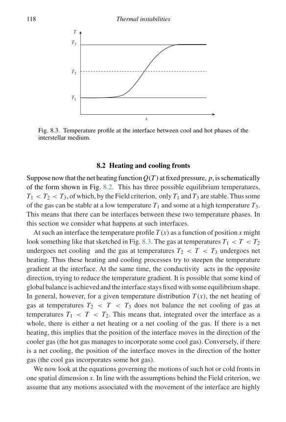
118 Thermal instabilities
x
T3
T
T2
T1
Fig. 8.3. Temperature profile at the interface between cool and hot phases of theinterstellar medium.
8.2 Heating and cooling fronts
Suppose now that the net heating function Q(T ) at fixed pressure, p, is schematicallyof the form shown in Fig. 8.2. This has three possible equilibrium temperatures,T1 < T2 < T3, of which, by the Field criterion, only T1 and T3 are stable. Thus someof the gas can be stable at a low temperature T1 and some at a high temperature T3.This means that there can be interfaces between these two temperature phases. Inthis section we consider what happens at such interfaces.
At such an interface the temperature profile T (x) as a function of position x mightlook something like that sketched in Fig. 8.3. The gas at temperatures T1 < T < T2
undergoes net cooling and the gas at temperatures T2 < T < T3 undergoes netheating. Thus these heating and cooling processes try to steepen the temperaturegradient at the interface. At the same time, the conductivity acts in the oppositedirection, trying to reduce the temperature gradient. It is possible that some kind ofglobal balance is achieved and the interface stays fixed with some equilibrium shape.In general, however, for a given temperature distribution T (x), the net heating ofgas at temperatures T2 < T < T3 does not balance the net cooling of gas attemperatures T1 < T < T2. This means that, integrated over the interface as awhole, there is either a net heating or a net cooling of the gas. If there is a netheating, this implies that the position of the interface moves in the direction of thecooler gas (the hot gas manages to incorporate some cool gas). Conversely, if thereis a net cooling, the position of the interface moves in the direction of the hottergas (the cool gas incorporates some hot gas).
We now look at the equations governing the motions of such hot or cold fronts inone spatial dimension x. In line with the assumptions behind the Field criterion, weassume that any motions associated with the movement of the interface are highly
8.2 Heating and cooling fronts 119
subsonic. Then we may neglect the velocity terms in the momentum equation inone dimension so that it becomes
∂p
∂x= 0, (8.18)
or equivalently p = const.In one dimension it is sensible to change to a Lagrangian variable m(x, t) defined
as follows:
m(x, t) =∫ x
−∞ρ(x′, t) dx′. (8.19)
Using the mass conservation equation, we can then show that
∂m
∂t
∣∣∣∣x
= −ρu, (8.20)
where u is the velocity in the x-direction. Hence we deduce that
∂
∂x
∣∣∣∣t= ρ
∂
∂m
∣∣∣∣t
(8.21)
and that∂
∂t
∣∣∣∣x
= ∂
∂t
∣∣∣∣m
− ρu∂
∂m
∣∣∣∣t. (8.22)
These show that the Lagrangian derivative, Df /Dt, for any quantity f becomes
∂f
∂t
∣∣∣∣x+ u
∂f
∂x
∣∣∣∣t= ∂f
∂t
∣∣∣∣m
. (8.23)
Using all these, the one-dimensional energy equation in the form
1
γ − 1
Dp
Dt− γ
γ − 1
p
ρ
Dρ
Dt= ∂
∂x
(λ∂T
∂x
)+ Q (8.24)
becomes
− γ
γ − 1
p
ρ
∂ρ
∂t
∣∣∣∣m
= ρ∂
∂m
(λρ
∂T
∂m
)+ Q. (8.25)
We now use the equation of state, p = (R/µ)ρT , together with the subsonicapproximation p = const., to eliminate ρ ∝ 1/T . Thus we can regard both λ andQ as functions of T alone. Then by scaling the time variable as follows:
τ = γ − 1
γ
p
(R/µ)2t (8.26)
and writing
L(T ) =(R/µ
p
)2 Q(T )
T, (8.27)
120 Thermal instabilities
the equation governing the evolution of the temperature front becomes
∂T
∂t= ∂
∂m
(λ(T )
T
∂T
∂m
)+ L(T ). (8.28)
A useful approximation is often to take λ(T ) ∝ Tα for some α (for example,conductivity by thermal electrons has α = 5/2 and conductivity by neutral ionshas α = 1/2). In this case, with suitable scaling, the energy equation becomes
∂T
∂t= ∂
∂m
(Tα−1 ∂T
∂m
)+ L(T ). (8.29)
For a steadily moving front, with velocity U in m-space, we can set ξ = m − Utand obtain an ordinary differential equation for T , regarding U as an eigenvalue.With the substitution T = Z1/α we have
Zβ d2Z
dξ2+ U
dZ
dξ+ F(Z) = 0, (8.30)
where β = (α − 1)/α and F(Z) = αTαβL(T ).
8.3 Further reading
A full description of the analysis presented here on the thermal stability of theinterstellar medium is given by Field (1965). A more general discussion andapplication of the evolution of heating and cooling fronts is given by Meerson(1996). Also of interest are the papers by Elphick, Regev & Spiegel (1991) andElphick, Regev & Shaviv (1992).
8.4 Problems
8.4.1 Show that the dispersion relation for linear waves propagating in a uniformcompressible gas with constant thermal conductivity λ is given by
iω(ω2 − k2c2s ) + λ(γ − 1)(k2T/p)[ω2 − k2c2
s /γ ] = 0. (8.31)
Show that the effect of a small thermal conductivity is always to damp travellingsound waves.
8.4.2 For a fluid with conductivity λ ∝ T , show that with suitable scalings aone-dimensional heating/cooling front satisfies the following equation:
∂T
∂t= ∂2T
∂m2+ L(T ), (8.32)
where m is the Lagrangian variable.If L = T (1 − T 2), show that there is a solution T (m) to this equation for which
the front is stationary. Sketch the solution and give physical reasons why the front isstationary in this case.
8.4 Problems 121
Show that a general steady solution of the equation extremises the functional
F[T ] =∫ [
1
2
(∂T
∂m
)2
+ U (T )
]dm, (8.33)
where we define L(T ) = −∂U/∂T , and that
∂T
∂t= −δF
δT, (8.34)
where δ/δT is the functional derivative.Show also that
dFdt
= −∫ (
δFδT
)2
dm (8.35)
and deduce that F is a Liapunov functional.Denoting the steady solution of the equation by T ∗(m), show that
d2T ∗
dm2= − d
dt∗[V (T ∗)], (8.36)
where we define V = −U .Note that eq. (8.36) is analogous to the equation of motion of a particle of unit
mass moving in a potential V . Hence show that if the net heating function is of theform L(T ) = T (1 − T 2) + A, where A is a constant, there is a steady front only ifA = 0. (See Elphick et al. (1991).)
8.4.3 The interstellar medium is modelled as a perfect gas, with equation of state p =RρT/µ, subject to cooling per unit volume at the rate ε(ρ, T ) = −ρ2�(T ) and withthermal conductivity λ(T ) = λ0Tα , where λ0 is a constant and α > 0. Gravity isneglected. Explain briefly the circumstances under which it is reasonable to assumethat the pressure remains uniform, i.e. ∇p = 0.
In this case, show that a planar one-dimensional flow obeys the following equation:
1
γ − 1
∂p
∂t+ γ
γ − 1p∂v
∂x+ ρ2� − ∂
∂x
(λ
∂T
∂x
)= 0, (8.37)
where v is the velocity in the x-direction.Show further that if the flow remains at constant pressure then
∂T
∂t+ v
∂T
∂x+(
γ − 1
γ
)(µ
R)2
p�(T )
T
−(
γ − 1
γ
)λ0T
p
∂
∂x
(Tα ∂T
∂x
)= 0.
Using the Lagrangian variable
m(x, t) =∫ x
0ρ(x, t) dx (8.38)
and an appropriately scaled time τ = Ct, where the constant C is to be determined,show that this equation can be written in the following form
∂T
∂τ+ �(T )
T= λ0
∂
∂m
(Tα−1 ∂T
∂m
)= 0. (8.39)
122 Thermal instabilities
At time t = 0, gas fills the half-space x > 0 and has uniform temperature T = T0.The region x < 0 contains cold (T = 0) infinitely dense gas which does not move butcools infinitely fast. The gas in x > 0 cools only by thermal conduction (i.e. � = 0if T > 0). Explain why it is reasonable to seek a similarity solution of the form
T (m, τ) = T0 f (ξ), (8.40)
with similarity variable ξ = m/(λTα−10 τ)1/2. Write down appropriate boundary
conditions for f (ξ) at ξ = 0 and as ξ → ∞.In the case when λ(T ) = λ0T , find the function f (ξ) in terms of the function
erf(z) = (2/√
π)∫ z
0 exp(−s2) ds, defined so that erf(∞) = 1.Sketch the resulting solution T (m, τ), indicating the behaviour as τ increases.Show that the rate L at which energy is radiated by the gas at x ≤ 0 varies as
L ∝ t−1/2.
9
Gravitational instability
In this chapter we consider instability driven by the self-gravity of the fluid. Thisis clearly an extremely important process whenever we deal with the formation ofbound objects such as stars and planets, and more generally large-scale structuresuch as galaxies and clusters.
9.1 The Jeans instability
To start with a simple picture we consider first a fluid at rest, with uniform densityρ and uniform pressure p, filling the whole of space. Then if we perturb the fluid,the linearized equation of motion is given by
∂u∂t
= −∇p′
ρ− ∇�′, (9.1)
where u is the fluid velocity , p′ is the Eulerian pressure perturbation and �′ isthe Eulerian perturbation of the gravitational potential �. The linearized massconservation equation is given by
∂ρ′
∂t+ ρ div u = 0, (9.2)
where ρ′ is the Eulerian density perturbation. The linearized version of Poisson’sequation, relating gravitational potential to mass density, is given by
∇2�′ = 4πGρ′. (9.3)
Assuming that the perturbations are adiabatic, the density and pressureperturbations are related through the following equation:
p′ = c2s ρ
′, (9.4)
where the sound speed cs is given by c2s = γ p/ρ.
123
124 Gravitational instability
Since the initial state is both uniform and at rest, we can Fourier analyze theseequations in both time and space, or equivalently we can take all linear quantitiesto have space and time dependence of the form exp{i(ωt + k · r)}.
Then, using eq. (9.4), eq. (9.1) becomes
iωu = −ikc2sρ′
ρ− ik�′, (9.5)
eq. (9.2) becomes
iωρ′
ρ+ ik · u = 0 (9.6)
and eq. (9.3) becomes−k2�′ = 4πGρ′. (9.7)
We now eliminate u by taking the scalar product of eq. (9.5) with k andsubstituting into eq. (9.6), and then we use eq. (9.7) to eliminate �′. This givesa single linear homogeneous equation for ρ′/ρ, whose coefficient then gives us thedispersion relation:
ω2 = k2c2s − 4πGρ. (9.8)
In the absence of gravity, i.e. setting G = 0, we recognize this relation as givingsimple acoustic waves, with sound speed cs. These are then modified by thepresence of gravity, which acts with a frequency ωG = (4πGρ)1/2, or equivalentlyacts on a timescale τG = 2π/ωG = (π/Gρ)1/2. If the gravity term becomes largeenough, which occurs at sufficiently large wavelengths that k2c2
s < 4πGρ, we seethat ω2 < 0 and instability sets in. The critical wavelength at which this occurs,that is the value of 2π/k at which ω2 = 0, is known as the Jeans length λJ givenby
λ2J = πc2
s
Gρ. (9.9)
We can also define a critical mass, called the Jeans mass, MJ = ρλ3J . This yields
MJ =(π
G
)3/2 c3s
ρ1/2. (9.10)
There is a simple physical interpretation of this result. Consider an element of thefluid of size ∼λ. Gravity acts on this fluid element to try to make it collapse on atimescale τG. In the other direction, the fluid element can use pressure to supportitself against gravity. But to do so the two sides of the fluid element need to be in(pressure) communication with each other. Since pressure communication occursat the speed of sound, the timescale on which the two sides can communicate isjust the sound crossing time for the element, i.e. τs = λ/cs. We then see fromthe above that τG = τs when λ = λJ. Thus for elements of size λ > λJ pressurecommunication cannot occur quickly enough to prevent gravitational collapse.
9.2 Isothermal, self-gravitating plane layer 125
Although the result we obtain from this analysis is a simple one and affords astraightforward physical explanation, the derivation of the result is flawed. Thereason for this is that the initial, unperturbed state was not in equilibrium, in thesense that it did not satisfy the unperturbed equations. The equations it did notsatisfy were the unperturbed Poisson equation,
∇2� = 4πGρ, (9.11)
together with the assumption that ∇� = 0 in the unperturbed state. If ρ is uniformand fills all space, then these conditions cannot be satisfied.
One tempting way out of this dilemma is to imagine that the results here mightapply to the very centre of a large mass of gas, where we might be able to takeapproximately p ≈ const., ρ ≈ const. and ∇� ≈ 0. Unfortunately, the timescaleon which the instability operates is exactly the timescale (∼1/
√Gρ) on which such
a cloud would collapse due to gravity. Thus no matter how large the cloud, from thepoint of view of looking at an instability, we cannot assume that the cloud is at rest.Problem 9.5.3 shows that perturbations of such collapsing flows grow algebraicallyrather than exponentially.
All is not lost, however. If we consider the fluid lying at the bottom of alarge shallow and fixed gravitational potential well caused by something else (forexample dark matter) then the fluid there does obey p ≈ const., ρ ≈ const. and∇� ≈ 0. Then in the region of the bottom of the well, the above analysis doesapply approximately to perturbations of short enough wavelength.
9.2 Isothermal, self-gravitating plane layer
At the present time in the Universe, star formation occurs mainly in the discs ofspiral galaxies. Thus it is important to consider the gravitational stability of a planelayer of gas. We consider first the equilibrium configuration.
9.2.1 Equilibrium configuration
We consider a layer of gas at rest and centred on the plane z = 0. The gas is uniformin the x- and y-directions and extends to infinity in both these directions. We takethe gas to be isothermal, so that the equation of state is simply p = ρc2
s , wherec2
s = const. Then hydrostatic equilibrium in the z-direction implies
1
ρ
dp
dz+ d�
dz= 0. (9.12)
We now define a variable m as follows:
m =∫ z
0ρ dz, (9.13)
126 Gravitational instability
which is simply the surface density of material between 0 and z. Then, also usingthe equation of state, the equation of hydrostatic equilibrium becomes
c2s
dρ
dm= −d�
dz. (9.14)
If we assume that the gravitational potential also depends only on z, Poisson’sequation is given by
d2�
dz2= 4πGρ. (9.15)
Combining these equations we eliminate � and obtain an equation for ρ as follows:
c2s
d2ρ
dm2= −4πG. (9.16)
We now impose the condition that ρ is symmetric above and below the z = 0 (orm = 0) plane and define the total surface density of the (half) layer as M , so that
M =∫ ∞
0ρ dz. (9.17)
Then the solution to eq. (9.16) is as follows:
ρ(m) = 2πGM 2
c2s
[1 −
( m
M
)2]
. (9.18)
In order to obtain the density structure as a function of physical height z, it isconvenient to define a quantity ξ
ξ = m
M. (9.19)
Then eq. (9.18) is simply given by
ρ(ξ) = ρ0(1 − ξ2), (9.20)
where ρ0 is the density on the midplane z = 0. Then since by definition ρ =dm/dz = M dξ/dz, we see that
Mdξ
dz= ρ0(1 − ξ2), (9.21)
which integrates as follows:
ρ0z = M tanh−1(ξ). (9.22)
We substitute for ξ in eq. (9.20) and, using the standard identity 1 − tanh2 x =sech2x, we find the equilibrium density structure of the layer as follows:
ρ(z) = ρ0sech2(z/H ), (9.23)
9.2 Isothermal, self-gravitating plane layer 127
where the scaleheight H is given by
H = M
2ρ0, (9.24)
or, using the definition of ρ0,
H = c2s
4πGM. (9.25)
We note that we have again side-stepped the issue of whether the equilibriumconfiguration can physically exist. The solution for the gravitational potential �(z)does not tend to a constant for large |z|. Instead, � → |z| as z → ±∞. So, onceagain, we cannot provide a fully self-consistent picture.
9.2.2 Stability analysis
We now consider small oscillatory perturbations to the self-gravitating layer of theform ∝ exp{i(ωt)}. The linearized equation of motion is given by
−ω2ξ = − 1
ρ∇p′ + ρ′
ρ2∇p − ∇�′. (9.26)
To avoid the complications of considering oscillations arising from buoyancy , weassume that the perturbations, like the equilibrium structure, are isothermal. Thisimplies that
p′ = c2s ρ
′, (9.27)
where c2s = const. Using this, the equation of motion is given by
−ω2ξ = −∇W − ∇�′, (9.28)
where we have defined
W = p′
ρ. (9.29)
Rather than looking for the general solution for the oscillation modes (stableand unstable) of the layer, we are interested in the critical point at which thelayer becomes unstable to self-gravity. From our earlier analysis (Chapter 4),we know from the ‘exchange of stabilities’ that as we pass from stable to unstableconfigurations, the quantity ω2 must pass through zero. Thus to find the criticalconfiguration on the border between stability and instability we can simply setω2 = 0. On doing this, we find that eq. (9.28) becomes
�′ = −W . (9.30)
We now substitute this into the linearized version of Poisson’s equation:
∇2�′ = 4πGρ′ (9.31)
128 Gravitational instability
and use the definition of W to obtain
∇2W + 4πGρ
c2s
W = 0. (9.32)
We consider modes of a particular wavelength λ = 2π/k in the horizontal direc-tion by Fourier analyzing in x and y, that is by writing W = W (z) exp{i(kxx+kyy)}.The equation then becomes
d2W
dz2+(
4πGρ(z)
c2s
− k2)
W = 0, (9.33)
where k2 = k2x + k2
y .In solving this equation we have to take account of the structure of the layer in the
z-direction. To do so we replace the independent variable z by ξ using eqs. (9.20)and (9.22). After a little algebra, we obtain the equation for W (ξ) as follows:
d2W
dξ2+ 2ξ
1 − ξ2
dW
dξ+[
2
1 − ξ2− kM /ρ0
(1 − ξ2)2
]W = 0. (9.34)
We now recall that the solutions of Legendre’s equation,
d2y
dx2+ 2x
1 − x2
dy
dx+[ν(ν + 1)
1 − x2− µ2
(1 − x2)2
]W = 0, (9.35)
which are non-singular at x = ±1, are called associated Legendre polynomialsdenoted by Pµ
ν (x). Their regularity requires that ν be a positive integer and that µ
be an integer in the range −ν ≤ µ ≤ ν.Thus in the equation for W (ξ) we see that ν = 1, and for non-zero k we require
µ = 1. This gives the critical wavenumber kJ = ρ0/M at which instability sets in.Using the definition of ρ0, we can write the critical wavenumber as follows:
kJ = 2πGM
c2s
. (9.36)
From our physical picture in Section 9.1 we expect that modes with k < kJ areunstable to self-gravity. In terms of the scaleheight of the layer, we see that modeswith wavelengths λ > λJ are unstable, where the Jeans length λJ is given by
λJ = 4πH . (9.37)
9.3 Stability of a thin slab
Seen from distances much larger than the scaleheight H , the layer discussedabove appears very thin and the internal structure of the layer becomes irrelev-ant. Moreover, we have found that the critical scalelength on which gravitational
9.3 Stability of a thin slab 129
instability sets in is many times H . Thus it also seems likely that the internalstructure of the layer does not play a critical role in determining the Jeans lengthλJ. For this reason, we now consider the stability of an infinitesimally thin slab offluid situated in the plane z = 0. Moreover, we are interested in motions due toself-gravity, and we expect these to be only in the plane of the slab.
As an equilibrium configuration we consider the slab to have constant surfacedensity �(x, y) = �0 = const. and constant pressure P(x, y) = P0 = const. Thenthe equilibrium gravitational potential is given by
�0 = −2πG�0|z|. (9.38)
Now we consider perturbations of the equilibrium of the form ∝ exp{i(ωt +kxx + kyy)}. The mass conservation equation is given by
∂�
∂t+ div(�u) = 0, (9.39)
where we recall that the velocity u is only in the (x, y)-plane. The linearized versionof this is then given by
iω�′ + ik · u�0 = 0. (9.40)
Similarly, the equation of motion given by
∂u∂t
+ u · ∇u = − 1
�∇⊥P − ∇⊥�, (9.41)
where the operator ∇⊥ acts only in the (x, y)-plane, linearizes to yield
iωu = − 1
�0ikP′ − ik�′, (9.42)
where we note that here �′ is evaluated on the plane z = 0.We take an adiabatic equation of state of the form
P = K�� , (9.43)
where K is a constant and � is the adiabatic exponent appropriate for twodimensions. We also assume adiabatic perturbations so that
P′ = C2s �′, (9.44)
where the two-dimensional sound speed, C2s , is given by C2
s = �P0/�0.Using this, we now combine eqs. (9.40) and (9.42) to eliminate u, and we obtain
−ω2�′ = k2C2s �′ + k2�0�
′. (9.45)
We now need to use Poisson’s equation to relate �′ and �′. Because the densityis confined to a thin slab, the linearized version of Poisson’s equation is given by
∇2�′ = 4πG�′δ(z), (9.46)
130 Gravitational instability
or equivalentlyd2�′
dz2= k2�′ + 4πG�′δ(z). (9.47)
Except on the plane z = 0, this has the following solution:
�′ = A exp(−|kz|), (9.48)
where A is a constant and we have imposed the condition that the perturbed potentialvanishes at large |z|. To determine the value of A, we integrate eq. (9.46) with respectto z from z = ε to z = −ε and then take the limit ε → 0. This gives the jump ind�′/dz across the z = 0 plane as[
d�′
dz
]0+
0−= 4πG�′. (9.49)
Hence we conclude that
�′(z = 0) = −2πG�′
|k| . (9.50)
We now substitute this into eq. (9.45) to obtain the dispersion relation:
ω2 = k2C2s − 2πG�0|k|. (9.51)
This has very similar properties to what we have found above. When gravity isnegligible (G = 0) we just get acoustic waves with speed Cs. As gravity becomesmore important, there is a critical value of the wavenumber kJ at which ω2 changessign and instability sets in. The wavenumber
kJ = 2πG�0
C2s
(9.52)
corresponds exactly to what we found in Section 9.2 for the isothermal gas layer.However, once again there are problems with this analysis because the self-
gravity of the equilibrium configuration in the (x, y)-direction is not properlyaccounted for. One way of providing a proper balance in the (x, y)-plane is to allowthe configuration to rotate. This has obvious astrophysical applications. Rotationallows us to set up a balance between gravity and centrifugal force and to providea fully self-consistent equilibrium. However, analysis of such a configurationwill have to wait until we have looked at the analysis of rotating shear flows inChapter 12.
9.4 Further reading
A simple description of the gravitational instability can be found in Jeans (1929,Chap. XIII). The stability of the isothermal self-gravitating plane layer is given byLedoux (1951).
9.5 Problems 131
9.5 Problems
9.5.1 Show that a self-gravitating, isothermal slab of gas (sound speed cs) centred on theplane z = 0 and immersed in a non-gravitating external medium with pressure pe
has a density profile ρ0(z), with midplane density ρ00, where
ρ0(µ) = ρ00(1 − µ2), (9.53)
µ = tanh(z/h) (9.54)
andh = cs/
√2πGρ00, (9.55)
valid for −A < µ < A, where A2 = 1 − pe/ρ00c2s .
If � is the surface density of the self-gravitating slab, show that
ρ00 = (2pe + πG�2)/2c2s . (9.56)
9.5.2 Consider a strongly compressed isothermal slab, such that pe ≈ ρ00c2s � G�2/2. In
this approximation, the pressure and density are almost constant throughout the slaband the slab extends in the range −a ≤ z ≤ a, where a = �/2ρ00 � h. Consider asmall perturbation of the slab with magnitude ξ , where ξ/a � a/h � 1. This impliesthat self-gravity may be ignored. Assume that the velocity of the perturbation is ofthe form u = (u, 0, w), that the perturbation is isothermal, so that p′ = c2
s ρ′ and that
the perturbed quantities have the following form:
p′(x, z, t) = p′(z) exp{i(ωt − kx)}. (9.57)
Assume a fixed pressure boundary condition p′(z = ±a) = 0. Show that thedispersion relation takes the form
ω2 = k2c2s + N 2π2c2
s
4a2(9.58)
for all integers N = 1, 2, 3, . . .Sketch the group velocity against wavenumber for the fastest propagating mode.
(See Doroshkevich (1980) and Lubow & Pringle (1993).)9.5.3 A large spherical cloud of gas of radius R0 is centred at the origin and has uniform
density ρ00 and zero pressure . At time t = 0 it begins to collapse from rest under itsown gravity. At time t the velocity field within the cloud may be written as follows:
u0(r, t) = r[
R(t)
R(t)
], (9.59)
where R(t) is the cloud radius and r is the radius vector from the origin. Show thatthe density remains uniform and that at time t it is given by
ρ0(t) = ρ00[R0/R(t)]3. (9.60)
Show that the gravitational force within the cloud is given by
g = −r[
4
3πGρ0(t)
](9.61)
132 Gravitational instability
and hence that
R2R = −4
3πGρ00R3
0. (9.62)
Show that the collapse is described implicitly by
R = 1
2R0(1 + cos φ) (9.63)
and
Ct = 1
2R0(φ + sin φ), (9.64)
where
C2 = 8
3πGρ00R2
0. (9.65)
As the cloud collapses (still with zero pressure) it is subject to small perturbations.Ignoring the effects of the cloud boundaries (or assuming the cloud is infinitely large),we assume that the perturbations take the form
ρ(r, t) = ρ0(t) + ρ′(r, t), (9.66)
with
ρ′(r, t) = ρ1(t) exp(ik · r) (9.67)
and where
k(t) = qR(t)
(9.68)
and q is independent of t. Explain briefly the physical motivation for such anassumption.
Using this assumption, show that the equation of mass conservation implies
ρ1 + 3ρ1R
R+ i
ρ0
Rq · u1 = 0, (9.69)
where u1(t) is the analogous velocity perturbation.Similarly, show that
u1 + R
Ru1 = −i
qR
�1, (9.70)
where �1 is the analogous perturbation to the gravitational potential, and that
− q2
R2�1 = 4πGρ1. (9.71)
Hence show that for compressive modes the fractional density perturbation, definedby δ(t) = ρ1(t)/ρ0(t), satisfies the following equation:
δ + 2R
Rδ − 4πGρ0(t)δ = 0. (9.72)
9.5 Problems 133
Show that one solution of this equation is given implicitly by
δ(φ) = sin φ
(1 + cos φ)2. (9.73)
By considering the behaviour of the solutions as R → 0, i.e. as φ → π , orotherwise, show that this is the only growing solution as the collapse proceeds. (SeeColes & Lucchin (1995) and Weinberg (1972).)
10
Linear shear flows
Shear flows are found in many areas of astronomy and occur whenever one fluidflows past another. An obvious place this occurs is when a jet flows into an ambientmedium. A shear flow occurs at the sides of the jet and this is usually unstable,leading to energy release and radiative emission. Shear is also a characteristicfeature of rotating discs. In this chapter we study the simplest case, where theshear flow is linear. Thus we consider flows whose unperturbed form in Cartesiancoordinates is given by
U(z) = (U (z), 0, 0). (10.1)
We can see the strong tendency towards instability in such flows by consideringa fluid of uniform density ρ lying between the two planes z = ±a, whose velocityprofile takes the form U (z) = U0(z/a), where U0 is a constant. The total linearmomentum of the fluid is zero. Thus, in principle, if there were some kind ofinstability which resulted in the fluid being completely mixed, the fluid would bebrought to rest. This process would release an amount of energy given by
�E =∫ a
−a
1
2ρU 2 dz = 1
2ρU 2
0 (10.2)
per unit length in the x-direction. This is a typical situation in which we can expecta fluid flow to be unstable. It occurs when some perturbation is able to tap an energysource of some kind (here the free shear energy ) while obeying the conservationlaws required by the fluid equations (here the conservation of linear momentum).
In this chapter we consider only incompressible fluids. This is a reasonableapproximation if the relative shear motions are subsonic. This is in fact often notthe case in astrophysical situations. However, if we included incompressibility wewould have to consider the added complication that the shear layer can lose energyby emitting acoustic waves. For the sake of simplicity we shall ignore this aspectof the problem.
134
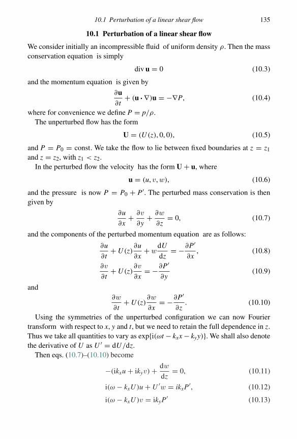
10.1 Perturbation of a linear shear flow 135
10.1 Perturbation of a linear shear flow
We consider initially an incompressible fluid of uniform density ρ. Then the massconservation equation is simply
div u = 0 (10.3)
and the momentum equation is given by
∂u∂t
+ (u · ∇)u = −∇P, (10.4)
where for convenience we define P = p/ρ.The unperturbed flow has the form
U = (U (z), 0, 0), (10.5)
and P = P0 = const. We take the flow to lie between fixed boundaries at z = z1
and z = z2, with z1 < z2.In the perturbed flow the velocity has the form U + u, where
u = (u, v, w), (10.6)
and the pressure is now P = P0 + P′. The perturbed mass conservation is thengiven by
∂u
∂x+ ∂v
∂y+ ∂w
∂z= 0, (10.7)
and the components of the perturbed momentum equation are as follows:
∂u
∂t+ U (z)
∂u
∂x+ w
dU
dz= −∂P′
∂x, (10.8)
∂v
∂t+ U (z)
∂v
∂x= −∂P′
∂y(10.9)
and∂w
∂t+ U (z)
∂w
∂x= −∂P′
∂z. (10.10)
Using the symmetries of the unperturbed configuration we can now Fouriertransform with respect to x, y and t, but we need to retain the full dependence in z.Thus we take all quantities to vary as exp{i(ωt − kxx − kyy)}. We shall also denotethe derivative of U as U ′ = dU/dz.
Then eqs. (10.7)–(10.10) become
−(ikxu + ikyv) + dw
dz= 0, (10.11)
i(ω − kxU )u + U ′w = ikxP′, (10.12)
i(ω − kxU )v = ikyP′ (10.13)
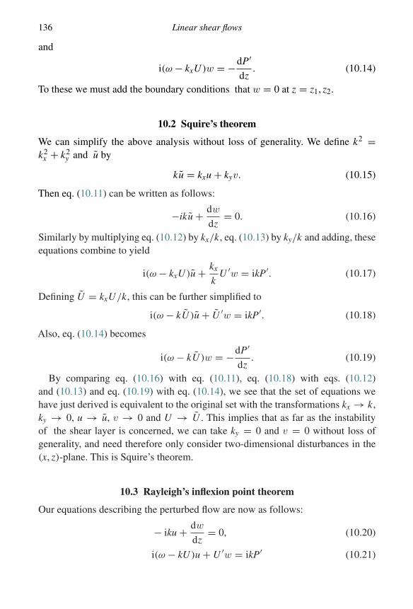
136 Linear shear flows
and
i(ω − kxU )w = −dP′
dz. (10.14)
To these we must add the boundary conditions that w = 0 at z = z1, z2.
10.2 Squire’s theorem
We can simplify the above analysis without loss of generality. We define k2 =k2
x + k2y and u by
ku = kxu + kyv. (10.15)
Then eq. (10.11) can be written as follows:
−iku + dw
dz= 0. (10.16)
Similarly by multiplying eq. (10.12) by kx/k, eq. (10.13) by ky/k and adding, theseequations combine to yield
i(ω − kxU )u + kx
kU ′w = ikP′. (10.17)
Defining U = kxU/k, this can be further simplified to
i(ω − kU )u + U ′w = ikP′. (10.18)
Also, eq. (10.14) becomes
i(ω − kU )w = −dP′
dz. (10.19)
By comparing eq. (10.16) with eq. (10.11), eq. (10.18) with eqs. (10.12)and (10.13) and eq. (10.19) with eq. (10.14), we see that the set of equations wehave just derived is equivalent to the original set with the transformations kx → k,ky → 0, u → u, v → 0 and U → U . This implies that as far as the instabilityof the shear layer is concerned, we can take ky = 0 and v = 0 without loss ofgenerality, and need therefore only consider two-dimensional disturbances in the(x, z)-plane. This is Squire’s theorem.
10.3 Rayleigh’s inflexion point theorem
Our equations describing the perturbed flow are now as follows:
− iku + dw
dz= 0, (10.20)
i(ω − kU )u + U ′w = ikP′ (10.21)
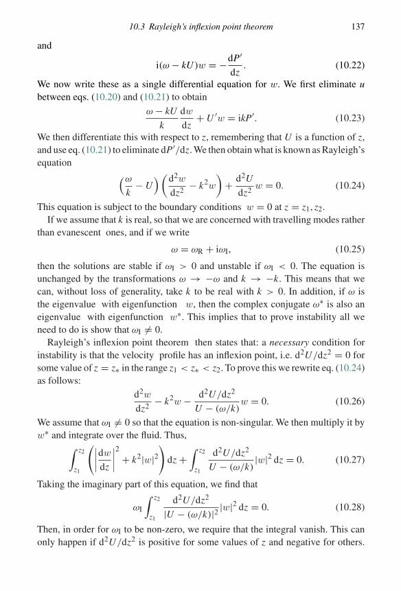
10.3 Rayleigh’s inflexion point theorem 137
and
i(ω − kU )w = −dP′
dz. (10.22)
We now write these as a single differential equation for w. We first eliminate ubetween eqs. (10.20) and (10.21) to obtain
ω − kU
k
dw
dz+ U ′w = ikP′. (10.23)
We then differentiate this with respect to z, remembering that U is a function of z,and use eq. (10.21) to eliminate dP′/dz. We then obtain what is known as Rayleigh’sequation (ω
k− U
)(d2w
dz2− k2w
)+ d2U
dz2w = 0. (10.24)
This equation is subject to the boundary conditions w = 0 at z = z1, z2.If we assume that k is real, so that we are concerned with travelling modes rather
than evanescent ones, and if we write
ω = ωR + iωI, (10.25)
then the solutions are stable if ωI > 0 and unstable if ωI < 0. The equation isunchanged by the transformations ω → −ω and k → −k. This means that wecan, without loss of generality, take k to be real with k > 0. In addition, if ω isthe eigenvalue with eigenfunction w, then the complex conjugate ω∗ is also aneigenvalue with eigenfunction w∗. This implies that to prove instability all weneed to do is show that ωI �= 0.
Rayleigh’s inflexion point theorem then states that: a necessary condition forinstability is that the velocity profile has an inflexion point, i.e. d2U/dz2 = 0 forsome value of z = z∗ in the range z1 < z∗ < z2. To prove this we rewrite eq. (10.24)as follows:
d2w
dz2− k2w − d2U/dz2
U − (ω/k)w = 0. (10.26)
We assume that ωI �= 0 so that the equation is non-singular. We then multiply it byw∗ and integrate over the fluid. Thus,∫ z2
z1
(∣∣∣∣dw
dz
∣∣∣∣2
+ k2|w|2)
dz +∫ z2
z1
d2U/dz2
U − (ω/k)|w|2 dz = 0. (10.27)
Taking the imaginary part of this equation, we find that
ωI
∫ z2
z1
d2U/dz2
|U − (ω/k)|2 |w|2 dz = 0. (10.28)
Then, in order for ωI to be non-zero, we require that the integral vanish. This canonly happen if d2U/dz2 is positive for some values of z and negative for others.
138 Linear shear flows
This means that there must be some point z = z∗ at which d2U/dz2 = 0, i.e. theremust be an inflexion point in the velocity profile.
10.3.1 Mathematical technicality
Equation (10.26) is formally singular for values of ω = kU (z) with z1 < z < z2.This implies that when we come to carry out formally the contour integration toinvert the Fourier transform and find the real solution as a function of time t, wemay not only have to evaluate the function at poles, which typically give rise toexponential behaviour, but also have to evaluate the integral along a cut on thereal ω-axis. When using Fourier transforms there is then some ambiguity as towhich side of the cut the contour should be drawn. For this reason it often makesmore physical sense to think in terms of solving the problem as an initial-valueproblem and so to use Laplace transforms. In this case it is clear where theinverse contour should be drawn. One then ends up with contour integrals arounda cut (or cuts) on the imaginary axis. Such contour integrals typically give rise toalgebraic, rather than exponential, time behaviour. We note here that in the aboveanalysis we have implicitly assumed that any instability has exponential behaviour,i.e. that the contributions from the poles in the complex ω-plane dominate. We have,however, not proved this, and so we have not discussed the stability or otherwiseof the ‘singular modes’ which correspond to the cut along the real ω-axis.
10.4 Fjørtoft’s theorem
There is a slightly more stringent necessary condition for instability known asFjørtoft’s theorem. This states that a necessary condition for instability is that if z∗is a point at which d2U/dz2 = 0, then there must be some value z0 in the rangez1 < z0 < z2 such that
d2U
dz2
∣∣∣∣z0
[U (z0) − U (z∗)] < 0. (10.29)
We prove this as follows. Take the real part of eq. (10.27). This yields∫ z2
z1
(d2U
dz2
)U − (ωR/k)
|U − ω/k|2 |w|2 dz = −∫ z2
z1
(∣∣∣∣dw
dz
∣∣∣∣2
+ k2|w|2)
dz < 0. (10.30)
Then, if we have instability (ωI �= 0), we can add to the l.h.s. of this equation aquantity which from eq. (10.28) we know to be zero, namely
[(ωR/k) − U (z∗)]∫ z2
z1
d2U/dz2
|U − ω/k|2 |w|2 dz = 0. (10.31)
10.5 Physical interpretation 139
When we do this, we obtain the following result:∫ z2
z1
(d2U
dz2
)U (z) − U (z∗)|U − (ω/k)|2 |w|2 dz < 0, (10.32)
which proves the theorem.
10.5 Physical interpretation
On the face of it, Rayleigh’s theorem and Fjørtoft’s theorem look like randomresults which have emerged by chance from the mathematics. But of course theremust be some physical reasons behind the results. The simplest way to think aboutthese results is in terms of vorticity. For the unperturbed flow (U (z), 0, 0), thevorticity is of the form ω = ∇ ∧ u = (0, ω(z), 0), where
ω(z) = dU
dz. (10.33)
In addition we are considering perturbations of the form
u = (u, 0, w). (10.34)
In an incompressible fluid the equations of motion imply an equation for theevolution of vorticity which takes the following form:
Dω
Dt= (ω · ∇)u. (10.35)
This implies that the vortex lines all lie parallel to the y-axis and are moved aroundin the (x, z)-plane. Thus they are all conserved in strength.
We have argued that in order to release free shear energy , and so producean instability, we need to interchange fluid elements in an appropriate manner.Rayleigh’s criterion tells us that in order to produce an instability there must bea point at which d2U/dz2 = 0, or equivalently there must be a point at whichdω/dz = 0. At this point there are neighbouring fluid elements which have thesame vorticity but different velocities. Mixing such fluid elements, and so releasingshear energy, is permitted by the fluid equations. Thus if dω/dz is zero at some point,we have the possibility of an instability.
In Figs. 10.1(a) and (b) we show two velocity profiles which do not havean inflexion point and so are stable under these considerations. In Figs. 10.1(c)and (d) we show two velocity profiles which do have inflexion points, and so, byRayleigh’s criterion, might show instability. The profile in Fig. 10.1(c), however,does not obey the necessary condition given by Fjørtoft’s theorem, and so is stable.In contrast, the profile in Fig. 10.1(d) does obey the additional criterion and so mightbe unstable. What is the basic physical difference between these two? Here againit is illuminating to consider the corresponding vorticity profiles ω(z) (Fig. 10.2).
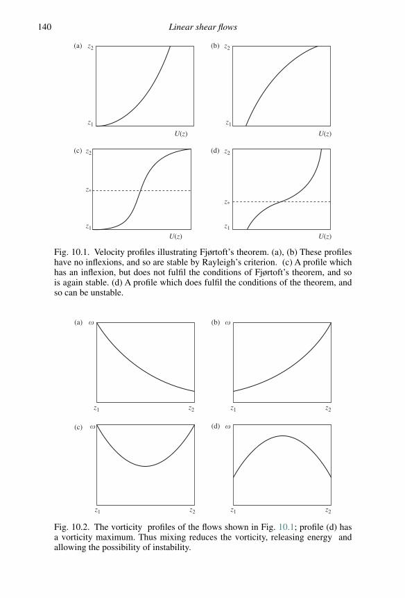
140 Linear shear flows
z2(a)
(c)
(b)
(d)
z2
z1
z2
z*
z1
z2
z*
z1
z1
U(z) U(z)
U(z)U(z)
Fig. 10.1. Velocity profiles illustrating Fjørtoft’s theorem. (a), (b) These profileshave no inflexions, and so are stable by Rayleigh’s criterion. (c) A profile whichhas an inflexion, but does not fulfil the conditions of Fjørtoft’s theorem, and sois again stable. (d) A profile which does fulfil the conditions of the theorem, andso can be unstable.
�(a)
(c)
(b)
(d)
�
� �
z2z1 z2z1
z2z1 z2z1
Fig. 10.2. The vorticity profiles of the flows shown in Fig. 10.1; profile (d) hasa vorticity maximum. Thus mixing reduces the vorticity, releasing energy andallowing the possibility of instability.
10.6 Co-moving phase 141
The energy which drives a shear instability derives from reducing the local shear,that is from reducing the local vorticity. At the same time, we know that from thevorticity equation the total vorticity of the fluid must be conserved. Moreover, theeffect of mixing neighbouring fluid elements is, on a coarse scale, to smooth outany vorticity profile. The profile shown in Fig. 10.1(c) has a vorticity profile with aminimum at z = z∗. The effect of mixing here is therefore to increase the vorticityat z∗. This does not release shear energy and so does not drive an instability. Incontrast, the profile shown in Fig. 10.1(d) has a vorticity profile with a maximum atz = z∗. The effect of mixing here is to reduce the local vorticity and so release shearenergy. Thus for this profile we have the possibility of a shear-driven instability.
10.6 Co-moving phase
We have so far looked at the properties the velocity profile of the fluid must havein order that there might be an instability. Here we look at the properties of theunstable mode. We start with Rayleigh’s equation (eq. (10.24)) in the form(
U − ω
k
) d2w
dz2−[
k2(
U − ω
k
)+ d2U
dz2
]w = 0. (10.36)
We now introduce a new variable ψ such that
ψ = w
U − (ω/k). (10.37)
Then Rayleigh’s equation becomes
d
dz
[(U − ω
k
)2 dψ
dz
]− k2
(U − ω
k
)2ψ = 0. (10.38)
We note in passing that this equation corresponds to a Sturm–Liouville problem inthat it comes from extremizing an integral in the form
δ
∫ z2
z1
(U − ω
k
)2[(
dψ
dz
)2
+ k2ψ2
]dz = 0. (10.39)
Returning to the main argument, we multiply eq. (10.38) by ψ∗ and integrateover the fluid to give∫ z2
z1
(U − ω
k
)2[∣∣∣∣dψ
dz
∣∣∣∣2
+ k2|ψ |2]
dz = 0. (10.40)
Taking the imaginary part of this equation, we then obtain
ωI
∫ z2
z1
(U − ωR
k
)[∣∣∣∣dψ
dz
∣∣∣∣2
+ k2|ψ |2]
dz = 0. (10.41)
142 Linear shear flows
We now see that for an unstable mode, for which we require ωI �= 0, there must bea point zp such that z1 < zp < z2 and ωR/k = U (zp). This means that an unstablemode must have a phase velocity equal to the fluid velocity at some point. Themode must co-move with some of the fluid. This also implies that some parts ofthe fluid move faster than the mode and some parts move slower. Thus, from aphysical point of view, the mode ‘knows’ about the shear and is in a position toallow communication between faster and slower moving fluid elements. It is thiscommunication which allows the mode to tap the shear energy, and so to grow.
10.7 Stratified shear flow
We now consider the situation in which a shear flow moves horizontally in a verticalgravitational field. Thus, as before, the unperturbed flow takes the following form:
U = (U (z), 0, 0), (10.42)
but now the unperturbed fluid has a density gradient ρ(z) and is subject to a uniformgravitational acceleration g = (0, 0, −g). For convenience we still assume that thefluid is incompressible. We take the velocity perturbation as (u, v, w).
From a physical point of view, the instability is now controlled by two physicaleffects. First, there is the free energy of the shear flow, which can be tapped toproduce growing modes. Second, there is the energy available from the gravitationalfield. In particular, if the fluid is stably stratified (here this implies dρ/dz < 0, sothat the heavier fluid is at the bottom) then the vertical mixing required to tap theshear energy needs to give up some of its energy to gravitation. Thus we expect thatinstability in this case arises as a balance between shear energy and gravitationalenergy.
As before, we Fourier transform the perturbation equations in the form ∝exp{i(ωt + kxx + kyy)}. The mass conservation equation div u = 0 yields
ikxu + ikyv + dw
dz= 0. (10.43)
Alternatively we can use Dρ/Dt = 0 to yield
i(ω + kxU )ρ′ + wdρ
dz= 0. (10.44)
These two equations are equivalent. Note that although the Lagrangian densityperturbation δρ is zero, the Eulerian density perturbation ρ′ is not. This is becausethere is a non-zero density gradient in the unperturbed fluid. Previously both dρ/dzand ρ′ were zero, and so the second equation was trivially satisfied.
10.7 Stratified shear flow 143
The three components of the linearized momentum equations are given by
i(ω + kxU )ρu + ρdU
dzw = −ikxp′, (10.45)
i(ω + kxU )ρv = −ikyp′ (10.46)
and
i(ω + kxU )ρw = −dp′
dz− gρ′. (10.47)
We now obtain an expression for u from eq. (10.45), namely
u = − kxp′
(ω + kxU )ρ− wU ′
i(ω + kxU ), (10.48)
and an expression for v from eq. (10.46), namely
v = − kyp′
(ω + kxU )ρ, (10.49)
and substitute them into eq. (10.43) to obtain an expression for p′ in terms of w andits derivative:
p′ = −i(ω + kxU )ρ
k2x + k2
y
dw
dz+ i
kxwρU ′
k2x + k2
yw. (10.50)
We also eliminate ρ′ between eqs. (10.47) and (10.44) to obtain an equation fordp′/dz in terms of w as follows:
dp′
dz= −i(ω + kxU )ρw − i
g(dρ/dz)
ω + kxUw. (10.51)
Combining eqs. (10.50) and (10.51) now gives a second-order differentialequation for w as follows:
d
dz
{(ω + kxU )ρ
dw
dz− kxρU ′w
}= k2⊥(ω + kxU )ρw + k2⊥g(dρ/dz)
ω + kxUw,
(10.52)
where we have written k2⊥ = k2x + k2
y .We now use physical intuition to make an approximation which, while not correct
in general, is justified for the purpose we have in mind. What we are looking forhere is not the general dynamical behaviour of the perturbed shear flow, but rathera stability criterion which gives us information about where the border betweenstability and instability lies. If we expand the l.h.s. of eq. (10.52) we obtain anumber of terms which contain the derivative dρ/dz. Now this derivative is related(eq. (10.46)) to the Eulerian density perturbation ρ′, and the change in local density
144 Linear shear flows
has two physical effects. First, it changes the local inertia of the fluid; that is,it changes the timescale on which the fluid reacts to a given force. Second, itchanges the local buoyancy of the fluid; that is, it changes the stability of the fluid.Since we are only interested in stability, and not in exact dynamical timescales,we can neglect the variation of ρ except where it is coupled to the gravity g. Inparticular, when expanding the derivative on the l.h.s. of eq. (10.52) we can treatρ as a constant.
This procedure yields the following equation:
(ω + kxU )
{d2w
dz2− k2⊥w
}− kx
d2U
dz2w − k2⊥
ω + kxU
(g
ρ
dρ
dz
)w = 0. (10.53)
As before, we now simply consider two-dimensional perturbations, so we takek⊥ = kx = k, and for convenience we define the phase velocity of the mode asc = ω/k. Then the equation becomes
(c + U )
(d2w
dz2− k2w
)− d2U
dz2w +
(−g
ρ
dρ
dz
)w
c + U= 0. (10.54)
This is called the Taylor–Goldstein equation.
10.8 The Richardson criterion
We are now in a position to obtain a necessary condition for the instability of thisstratified shear flow in a gravitational field.
We first define a quantity H as follows:
H = w
(c + U )1/2. (10.55)
In terms of this variable, eq. (10.54) becomes
d
dz
[(U+c)
dH
dz
]− k2(c + U )H − 1
2
d2U
dz2H −
{1
4U ′2−
[g
ρ
(−dρ
dz
)]}H
c + U= 0.
(10.56)
Note that for the fluid to be stably stratified in the absence of shear, we require that−dρ/dz > 0.
We now multiply this equation by the complex conjugate H∗ and integrate overthe fluid (from z1 to z2). We integrate by parts where necessary, using the boundaryconditions that w = 0 at z = z1, z2. We then obtain the following equation:∫ z2
z1
[{∣∣∣∣dH
dz
∣∣∣∣2
+k2|H |2}
+1
2
d2U
dz2|H |2 +
{1
4U ′2−
[g
ρ
(−dρ
dz
)]} |H |2c+U
]dz = 0.
(10.57)
10.10 Problems 145
Now we write c in terms of real and imaginary parts,
c = cR + icI, (10.58)
and note, as before, that for instability we just require that cI �= 0. Therefore wetake the imaginary part of eq. (10.57), which is as follows:
cI
∫ z2
z1
[∣∣∣∣dH
dz
∣∣∣∣2
+ k2|H |2 +{g/ρ (−dρ/dz) − U ′2/4
}|c + U |2
]dz = 0. (10.59)
We see by inspection that if throughout the fluid, i.e. in z1 < z < z2, we have
1
4U ′2 <
[g
ρ
(−dρ
dz
)], (10.60)
then the integrand is positive definite; therefore to satisfy the equation we requirecI = 0. Thus if the inequality eq. (10.60) is satisfied throughout the fluid, then theshear flow must be stable. This is known as the Richardson criterion. Physicallyspeaking, the l.h.s. is a measure of the energy available in the shear and the r.h.s.is a measure of the energy required to overturn the density gradient in the presenceof gravity. Thus the criterion states roughly that if there is not enough shear energyto overturn the density gradient then the fluid is stable. Note that the criterion onlygoes one way. It does not demonstrate instability if the inequality is not satisfied.
10.9 Further reading
A detailed discussion of the theory of the stability of incompressible shear flows isto be found in Drazin & Reid (1981, Chap. 4). Basic results about the Richardsoncriterion are given by Howard (1961) and Miles (1961). Consideration of the effectsof buoyancy, surface tension and magnetic fields can be found in Chandrasekhar(1961, Chap. XI). The complications introduced by consideration of compressibilityand the emission of acoustic waves from the shear layer are discussed by Gerwin(1968).
10.10 Problems
10.10.1 A smooth pipe with square cross section of side a lies flat on a horizontal surfacein the uniform gravitational field g. The pipe contains incompressible fluid.
(i) Consider the case where the fluid in the upper half of the pipe has densityρ1 and that in the lower half-pipe has density ρ0, where ρ1 > ρ0. What isthe physical origin of the instability which ensues? Calculate the energy E1
available to drive the instability per unit length of the pipe.(ii) Now consider the case where ρ1 < ρ0, but with the fluid in the upper half-
pipe moving with velocity V and the fluid in the lower half-pipe moving
146 Linear shear flows
with velocity −V . If we neglect gravity, setting g = 0, what is the physicalorigin of the instability which ensues? Show that the energy available to theinstability, per unit length of pipe, is given by
E0 = ρ0ρ1
ρ20 + ρ2
1
a2V 2. (10.61)
(iii) If now ρ1 < ρ0, but g �= 0, explain by comparing E0 and E1 the physicalsignificance of the Richardson number, Ri, where
Ri = ρ0ρ1
ρ20 − ρ2
1
V 2
ag. (10.62)
10.10.2 Consider a horizontal flow of incompressible fluid in a vertical, constantgravitational field g, so that
u ={
(U2, 0, 0), z > 0,
(U1, 0, 0), z < 0,(10.63)
ρ ={
ρ2, z > 0,
ρ1, z < 0(10.64)
and
p(z) ={
p0 − gρ2z, z > 0,
p0 − gρ1z, z < 0.(10.65)
Consider small perturbations, such that the interface of the fluid is at z = ζ(x, y, t),which leave the flow unperturbed as |z| → ∞. Assume that the perturbed flow isirrotational (zero vorticity) so that, for example, the flow in z > 0 can be writtenin terms of a velocity potential u = ∇φ2, where φ2 = U2x + φ′
2 and ∇2φ′2 = 0.
Show that the velocity potential obeys the following equation:
∂φ
∂t+ 1
2(∇φ)2 + p
ρ+ gz = const. (10.66)
Take the perturbed quantities to be of the form
φ′2 = φ2(z) exp{i(kx + ωt)} (10.67)
and find expressions for φ1 and φ2.Show that the dispersion relation of the perturbations is given by
ω2(ρ1 + ρ2) + 2ωk(ρ2U2 + ρ1U1) + k2(ρ2U 22 + ρ1U 2
1 ) + (ρ2 − ρ1)kg = 0.(10.68)
Discuss what happens when U1 = U2 = 0 in the two cases (i) ρ1 < ρ2,(ii) ρ1 > ρ2.
Show that if U1 �= U2 the flow is always unstable for perturbations of shortenough wavelength. (See Drazin & Reid (1981, Chap. 1).)
10.10 Problems 147
10.10.3 An incompressible fluid of uniform density ρ has a uniform magnetic field(in Cartesian coordinates) B0 = (B, 0, 0) and a shearing velocity field u0 =(U (z), 0, 0).
The flow is subject to small perturbations of the form
u = u0 + [u(z), v(z), w(z)] exp{i(ωt + kxx + kyy)}, (10.69)
B = B0 + [bx(z), by(z), bz(z)] exp{i(ωt + kxx + kyy)} (10.70)
and
p = p0 + p1(z) exp{i(ωt + kxx + kyy)} (10.71)
From the linearized equation of motion, show that
iρ(ω + kxU )w − B
(ikxbz − dbx
dz
)= −dp1
dz(10.72)
and derive the corresponding equations for u and v.From the linearized induction equation, show that
bx = kxB
ω + kxU
{u − iU ′w
ω + kxU
}, (10.73)
where U ′ = dU/dz, and obtain analogous expressions for by and bz in terms ofthe perturbed velocity components.
Substitute these expressions for the perturbed components of the magnetic fieldinto the linearized equations of motion.
From the x- and y-components of the linearized equations of motion, show thatthe z-component of the vorticity, ζ = ikxv − ikyu, is given by
ζ = kyU ′wω + kxU
. (10.74)
Deduce that the y-component of the linearized equation of motion simplifies to
iρ(ω + kxU )v = −ikyp1. (10.75)
Use div u = 0 to show that
ik2p1 = ρ(ω + kxU )dw
dz− ρkxU ′w, (10.76)
where k2 = k2x + k2
y .Combine div u = 0 with the expression for ζ to show that
ik2u = −[
kxdw
dz+ k2
y U ′
ω + kxUw
]. (10.77)
Hence, or otherwise, obtain an equation for w in the following form:
d
dz
{ρ(ω + kxU )
dw
dz− ρkxU ′w
}= k2ρ(ω + kxU )w
+ k2x B2
{d
dz
(dw/dz
ω + KxU
)− k2w
ω + kxU
}− k3
x B2 d
dz
{U ′w
(ω + kxU )2
}.
148 Linear shear flows
Consider a shear layer at z = 0, so that
U (z) ={
U2, z > 0,
U1, z < 0,(10.78)
where U1 and U2 are constants. Show that in this case the solutions of eq. (10.78)for which w/(ω + kxU ) is continuous and obey suitable boundary conditions asz → ±∞ are given by
w ={
A(ω + kxU2)e−kz , z > 0,
A(ω + kxU1)ekz , z < 0,(10.79)
for some constant A and for k > 0.By integrating eq. (10.78) from z = −ε to z = ε and letting ε → 0, show that
ρ(ω + kxU2)2 + ρ(ω + kxU1)
2 = 2k2x B2. (10.80)
Deduce that the shear flow is stable if (U1 − U2)2 < 4B2/ρ. Why does the
presence of this magnetic field tend to stabilize the shear flow? (See Chandrasekhar(1961, Chap. XI).)
10.10.4 A uniform density, incompressible fluid contains a bounded shear layer withvelocity field, in Cartesian coordinates, of the form U0 = (U (z), 0, 0), where
U (z) =
⎧⎪⎨⎪⎩
U0, z ≥ d ,
(z/d)U0, |z| < d ,
−u0, z ≤ −d .
(10.81)
It is subject to a perturbation of the form
u(x, z, t) = (u(z), 0, w(z)) exp{ik(x − ct)} (10.82)
and
p′(x, z, t) = p′(z) exp{ik(x − ct)}, (10.83)
where k > 0 is real. Obtain an equation for w(z) and show that an appropriatesolution is of the form
w(z) =
⎧⎪⎪⎨⎪⎪⎩
A exp[−k(z − d)], z ≥ d ,
B exp[−k(z − d)] + C exp[k(z + d)], |z| < d ,
D exp[k(z + d)], z ≤ −d ,
(10.84)
where A, B, C and D are constants.Explain why the quantity [
(c − U )dw
dz+ dU
dzw
](10.85)
is continuous at z = ±d .
10.10 Problems 149
Hence, or otherwise, show that(c
U0
)2
= 1
4α2{(2α − 1)2 − e−4α}, (10.86)
where α = kd .Deduce that disturbances with wavelengths such that 0 < α < αs are unstable
for some number αs, which is in the range 12 < αs < 1.
Give a physical interpretation of this result. (See Drazin & Reid (1981,Chap. 23).)
11
Rotating flows
Almost all astronomical objects rotate. The formation of astronomical objectsoften involves gravitational collapse over many orders of magnitude in size.Conservation of angular momentum then ensures that newly formed objects oftenrotate rapidly in the sense that rotational (centrifugal) forces play a dynamical role.In this and the next few chapters we consider the effects of rotation. In doing sowe shall have in mind mainly the effects of rotation on stellar objects, but note thatsome of our findings are also relevant to other types of object.
11.1 Rotating fluid equilibria
We begin by asking what kinds of equilibrium are possible for a rotating self-gravitating fluid mass. We consider a fluid rotating at a steady rate about an axis ofsymmetry. In cylindrical polar coordinates (R, φ, z), the flow velocity is given by
u = (0, uφ , 0), (11.1)
where uφ = R� is independent of the azimuthal coordinate φ and � is the angularvelocity. Since the flow is axisymmetric (∂/∂φ = 0), there are only two non-zerocomponents of the equation of hydrostatic equilibrium. Denoting the gravitationalpotential as �, the R-component is given by
−u2φ
R= − 1
ρ
∂p
∂R− ∂�
∂R(11.2)
and the z-component is given by
0 = − 1
ρ
∂p
∂z− ∂�
∂z. (11.3)
This can be written in differential form as follows:dp
ρ= gR dR + gz dz, (11.4)
150
11.2 Making rotating stellar models 151
where the vector g is given by
g =(
−∂�
∂R+ R�2, 0, −∂�
∂z
). (11.5)
The r.h.s. of this equation is the gradient of a scalar if and only if
∂gz
∂R= ∂gR
∂z, (11.6)
which is true if and only if
∂�
∂z= 0. (11.7)
If this holds, so that � is a function of R only, we may define an effective gravitationalpotential �e as follows:
�e = �(R, z) −∫ R
�2R dR. (11.8)
Then the effective gravity ge can be defined as
ge = −∇�e, (11.9)
and the equation of hydrostatic equilibrium becomes
∇p
ρ= ge. (11.10)
We note in passing that if the rotation is uniform, i.e. � = �0 = const., then
�e = � − 1
2R2�2
0. (11.11)
Returning to the general case, � = �(R), we see that hydrostatic equilibrium,expressed as
∇p = −ρ∇�e, (11.12)
means that ∇p and ∇�e are everywhere parallel. Thus p must be a function of �e,i.e. p = p(�e). Then, since ∇p/ρ = −∇�e, we have that ρ = dp/d�e is also justa function of �e. Hence we must have p = p(ρ), so the fluid is barotropic . Wehave shown therefore that
� = �(R) ⇔ p = p(ρ). (11.13)
11.2 Making rotating stellar models
The work in Section 11.1 shows that our freedom in building a model of a rotatingstar is severely reduced when we try to make simplifying assumptions. We have
152 Rotating flows
seen that to make a star which rotates uniformly (or one which rotates on cylinders)hydrostatic equilibrium requires the fluid to be barotropic . In addition, both pressurep and density ρ are functions only of the effective gravitational potential �e. If asusual the stellar gas obeys a perfect gas equation of state, we have p ∝ ρT andthe temperature also is just a function of �e.
The energy equation is given by
ρTDs
Dt= ρεnuc − div F, (11.14)
where εnuc is the nuclear energy generation rate per unit mass and F is the heatflux. In a steady state, where there are no velocities other than the rotational velocityuφ , this reduces to
div F = ρεnuc. (11.15)
If energy transport is by radiation, then
F = −χ∇T , (11.16)
where
χ = 4acT 3
3κρ, (11.17)
where a is the radiation energy density constant and c is the speed of light. Theopacity κ(ρ, T ) is a function of local fluid properties, and is also therefore just afunction of �e. This means that we can write
F = f (�e)∇�e, (11.18)
where the function f (�e) is given by
f (�e) = −4acT 3
3κρ
dT
d�e. (11.19)
At the stellar surface, p → 0 and ρ → 0, and therefore �e → �s where �s isthe constant surface value of the effective potential. This means that on the stellarsurface the radiative flux is proportional to the local surface gravity:
F ∝ ∇�e ∝ ge. (11.20)
Since by definition the effective temperature Te of the surface is given by theblackbody law, F = σT 4
e , where σ = ac/4 is the Stefan–Boltzmann constant,we have finally that
Te ∝ g1/4e . (11.21)
This is known as von Zeipel’s law of gravity darkening. It implies that thetemperature is not uniform over the surface of a rotating star, the equator being
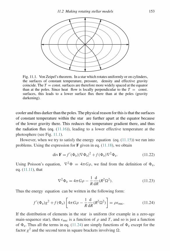
11.2 Making rotating stellar models 153
Fig. 11.1. Von Zeipel’s theorem. In a star which rotates uniformly or on cylinders,the surfaces of constant temperature, pressure, density and effective gravitycoincide. The T = const. surfaces are therefore more widely spaced at the equatorthan at the poles. Since heat flow is locally perpendicular to the T = const.surfaces, this leads to a lower surface flux there than at the poles (gravitydarkening).
cooler and thus darker than the poles. The physical reason for this is that the surfacesof constant temperature within the star are further apart at the equator becauseof the lower gravity there. This reduces the temperature gradient there, and thusthe radiation flux (eq. (11.16)), leading to a lower effective temperature at thephotosphere (see Fig. 11.1).
However, when we try to satisfy the energy equation (eq. (11.15)) we run intoproblems. Using the expression for F given in eq. (11.18), we obtain
div F = f ′(�e)|∇�e|2 + f (�e)∇2�e. (11.22)
Using Poisson’s equation, ∇2� = 4πGρ, we find from the definition of �e,eq. (11.11), that
∇2�e = 4πGρ − 1
R
d
dR(R2�2). (11.23)
Thus the energy equation can be written in the following form:
f ′(�e)g2 + f (�e)
[4πGρ − 1
R
d
dR(R2�2)
]= ρεnuc. (11.24)
If the distribution of elements in the star is uniform (for example in a zero-agemain-sequence star), then εnuc is a function of ρ and T , and so is just a functionof �e. Thus all the terms in eq. (11.24) are simply functions of �e except for thefactor g2 and the second term in square brackets involving �.
154 Rotating flows
If the rotation is uniform, � = �0 = const., then the rotational term is equalto 2�2
0, which is a constant. In this case, for the equation to be satisfied for allvalues of �e, i.e. everywhere in the star, we must demand that f ′(�e) = 0, i.e. thatf (�e) = const. From the definition of f , we see that this is true only if κ ∝ T 3/ρ.This is not true in general. If the rotation is not uniform, the same applies, andin addition, in order to make the term in square brackets depend only on �e (so thatwe can equate this to the r.h.s.), we require further that
1
R
d
dR(�2R2) = const. (11.25)
This implies that � takes the form
�2 = C1 + C2
R2, (11.26)
where C1 and C2 are constants. However, then in order that � is finite throughoutthe star, we require C2 = 0, and therefore that � = const. The energy equationthen implies that εnuc take the following form:
εnuc ∝(
1 − �2
2πGρ
), (11.27)
which is also not true in general.To summarize: so far we have seen that for a uniformly rotating star, hydrostatic
equilibrium implies that the stellar gas is barotropic (i.e. p = p(ρ)). Theimposition of radiative equilibrium then leads to contradictions. Thus stars eitherhave non-uniform rotation, or are not in radiative equilibrium.
11.3 Meridional circulation
The standard solution to this problem is to assume that the heat flux within the staris carried not only by conduction (radiative transfer) but is also transported bya steady circulation current in the meridional plane. The fluid flow within the starthen has an additional component of the form
u(R, z) = (uR, 0, uz). (11.28)
Then the energy equation becomes
ρTu · ∇S = div(χ∇T ) + ρεnuc, (11.29)
and we must also ensure mass conservation by taking
div(ρu) = 0. (11.30)
If the star is not rotating too fast, so that the quantity η = �2R3/GM is small,the standard procedure is to expand the equations in terms of η. There are now
11.3 Meridional circulation 155
enough degrees of freedom to solve for the meridional circulation u, and we referthe reader in Section 11.5 to the various textbooks in which this procedure is carriedout. Note that if there is no rotation, η = 0, there is no problem and we can takeu = 0. Thus we expect the magnitude of u to be proportional to η. From eq. (11.29)we may estimate the velocity required to carry a heat flux η times that transportedby conduction. To order of magnitude, we see that
ρTuS
R∼ η
1
R
L
R2. (11.31)
Here L is the stellar luminosity, and we have approximated the thermally conductedflux as χ∇T ∼ L/R2. Now the thermal energy content of the star is ∼R3ρTS,and by the virial theorem for an equilibrium star we can equate this, to orderof magnitude, to the gravitational self-energy ∼GM 2/R. Putting this together,we find
u ∼ ηLR2
GM∼ η
R
tKH. (11.32)
Here tKH is the time taken for a star to radiate away its thermal (or gravitational)energy . This Kelvin–Helmholtz timescale is around 30 million years for the Sun.The circulation timescale R/u is known as the Eddington–Sweet circulation timeand is therefore given roughly by
tES ∼ tKH/η. (11.33)
The solar rotation period is around 30 days, and thus for the Sun η ∼ 1/3000. Theresulting circulation timescale, tES ∼ 1011 years, exceeds the age of the Universe.However for faster-rotating stars the circulation timescale can become comparableto the timescale for nuclear evolution. Meridional circulation can in principlemove nuclear fuel around within such stars, and so can, again in principle, have asignificant influence on the star’s evolution.
11.3.1 The basic snag with meridional circulation
There is a fundamental problem with the standard procedure outlined above, whichis well known to those in the field. We ran into a snag in trying to construct a modelof a rotating star because we found that if we assumed that the star rotates uniformly,then it cannot also transport heat solely by conduction. The ‘meridional circulation’solution to this is to assume the existence of a meridional flow which transports heat.The basic problem with this approach arises because the assumed meridional flowwould also advect angular momentum. This then leads to the star no longer beingin uniform rotation. Moreover, since we have assumed that the motions are steady,the postulated existence of a meridional flow requires a corresponding process
156 Rotating flows
neutralizing the advection of angular momentum by the flow, by transporting itback at the same rate as it is advected by the flow. For this to happen the star mustbecome differentially rotating, so that � = �(R, z), and there must be dissipativeprocesses such as turbulence, magnetic field or convection which, when combinedwith the shear flow, can transport angular momentum in the right direction and atthe right rate.
Garaud (2002) shows that this can be achieved for a simple molecular viscosity. For realistic stellar transport processes the details have yet to be worked out, andit has yet to be demonstrated that such a solution occurs in practice in real stars.Assuming, however, that something like this does actually occur, we may tentativelyconclude that a rotating star is likely to be differentially rotating and that it willcontain circulation currents of some sort. However, whether these currents are ableto mix nuclear fuel, and so affect the stellar evolution, depends on unknown anduncertain dissipative processes within the star which determine the detailed, and asyet unknown, structure of the velocity field.
11.4 Rotation and magnetism
We have seen that the structure of a rotating star must in reality be quite complexbecause simple assumptions force unphysical constraints on the star. Somethingsimilar happens when we consider rotating stars with magnetic fields, as thefollowing result shows. In a differentially rotating fluid, a steady magnetic fieldconfiguration exists only if the magnetic field lines lie along surfaces of constantangular velocity. This is Ferraro’s law of isorotation.
To see this, suppose that the fluid rotates differentially with angular velocity�(R, z). Any magnetic field is advected by the fluid flow, and thus it is immediatelyapparent that the azimuthal field component, Bφ , is unaffected by the rotation.We may therefore simply consider a poloidal field of the form
B(R, z) = (BR, 0, Bz). (11.34)
From the induction equation, we know that a steady field obeys
curl(u ∧ B) = 0. (11.35)
The φ-component of this equation is given by
∂
∂z(uφBz) + ∂
∂R(uφBR) = 0. (11.36)
Using the fact that uφ = R�, this may be written in the form
∂
∂z(�Bz) + 1
R
∂
∂R(R�BR) = 0. (11.37)
11.6 Problems 157
We now note that this equation is div (B�) = 0, which when coupled with theMaxwell equation, div B = 0, implies that
B · ∇� = 0. (11.38)
Thus the magnetic field must lie at right angles to the gradient of the angularvelocity; that is, the field lines must lie along the surfaces of constant angularvelocity. On reflection, this is an obvious result. If a field line is such that differentpoints on it have different angular velocities, then the field line will eventuallytwist up, creating an azimuthal magnetic field. Thus it cannot be in a steady state.
11.5 Further reading
A more detailed description of the theory of rotating stars can be found in the worksof Tassoul (1978, 2000). A clear description of what is involved in the computationof meridional circulation in a simple idealized case is given by Garaud (2002).
11.6 Problems
11.6.1 Derive the equation of motion of an inviscid barotropic fluid subject to aconservative force field in a frame rotating with constant angular velocity �.
Show that in the rotating frame∫S(ω + 2�) · dS = const., (11.39)
where S is a surface spanning a closed contour � which moves with the fluid andwhere ω = curl u, where u is the velocity in the rotating frame. (See Greenspan(1968, Chap. 1).)
11.6.2 An incompressible fluid moves steadily and slowly in a frame rotating with constantangular velocity �. Taking appropriate approximations, show that
(� · ∇)u = 0. (11.40)
What does this result imply physically? (This is the Taylor–Proudman theorem;see Greenspan (1968, Chap. 1).)
12
Circular shear flow
In this chapter we shall consider the stability of a differentially rotating fluid. Clearlythis is directly relevant to important subjects in astrophysics, such as accretiondisc stability and galactic structure. As before we shall consider some particularexamples which serve to illustrate the relevant physical considerations.
12.1 Incompressible shear flow in a rigid cylinder
We consider first a rotating flow of an incompressible fluid within rigid cylindricalwalls. Thus the density ρ = const. and the unperturbed flow has a velocity fieldin cylindrical coordinates (R, φ, z) of the form
u0 = (0, V (R), 0), (12.1)
where the azimuthal velocity V (R) is related to the angular velocity �(R) by
V (R) = R�(R). (12.2)
For such a flow, with fluid velocity u = (uR, uφ , uz), the equations of motionare given by
∂uR
∂t+ u · (∇uR) − u2
φ
R= − 1
ρ
∂p
∂R, (12.3)
∂uφ
∂t+ u · (∇uφ) + uφuR
R= − 1
Rρ
∂p
∂φ(12.4)
and
∂uz
∂t+ u · (∇uz) = − 1
ρ
∂p
∂z. (12.5)
158
12.1 Incompressible shear flow in a rigid cylinder 159
In addition, we require the mass conservation equation, which for an incompressiblefluid is just given by
∂uR
∂R+ uR
R+ 1
R
∂uφ
∂φ+ ∂uz
∂z= 0. (12.6)
We note that since ρ is constant, the equilibrium pressure distribution is (fromeq. (12.3)) simply given by
p(R) = ρ
∫V 2
RdR. (12.7)
We perturb this solution, so that the velocity field becomes
u = (u′R, V (R) + u′
φ , u′z). (12.8)
To simplify notation we drop the primes from the first-order quantities. We musttherefore note that uφ is now the perturbation to the azimuthal velocity. We alsonote that there is no perturbation to the density, and for convenience we define thequantity
W = p′
ρ. (12.9)
To first-order in small quantities, the equations of motion are given by
∂uR
∂t+ V
R
∂uR
∂φ− 2Vuφ
R= −∂W
∂R, (12.10)
∂uφ
∂t+ V
R
∂uφ
∂φ+(
V
R+ dV
dR
)uR = − 1
R
∂W
∂φ(12.11)
and∂uz
∂t+ V
R
∂uz
∂φ= −∂W
∂z. (12.12)
We note that the mass conservation equation, eq. (12.6), is already linearized.Since the equilibrium configuration is independent of time, and of φ and z, we
may now Fourier analyze in t, φ and z. Thus we assume that all the linear variablesare of the form
p′(R, φ, z, t) → p′(R) exp{i(ωt + mφ + kz)}. (12.13)
In addition, we note that to keep p′ a single-valued function of azimuth φ we requirethat m is an integer. It is also convenient to define a quantity σ(R) which correspondsto the local Doppler-shifted frequency†
σ(R) = ω + m�(R). (12.14)
† It is important to remember that σ is a function of radius R. In our experience, errors in algebra often occurbecause this fact is forgotten.
160 Circular shear flow
The linearized equations are now as follows:
iσuR − 2�uφ = −dW
dR, (12.15)
iσuφ +[� + d
dR(R�)
]uR = − imW
R, (12.16)
iσuz = −ikW (12.17)
and
duR
dR+ uR
R+ imuφ
R+ ikuz = 0. (12.18)
We now write the equations in terms of the Lagrangian displacement ξ . Fromeq. (4.24) in Chapter 4 we recall that if the unperturbed fluid has a flow field u0,then the Eulerian velocity perturbation u′ is given in terms of ξ by
u′ = ∂ξ
∂t+ u0 · ∇ξ − ξ · ∇u0. (12.19)
In the case we are considering, with the unperturbed velocity field in theazimuthal direction and dependent only on radius R, we find that
uR = iσξR (12.20)
and
uz = iσξz. (12.21)
However, the azimuthal component takes a little more care, and we find that
uφ = iσξφ − Rd�
dRξR. (12.22)
Thus the underlying shear flow implies that uφ �= iσξφ . The added complicationto ξφ is necessary to ensure that when we write the mass conservation equation,eq. (12.18), in terms of ξ we obtain what is obviously the correct physical result:
div ξ = 0. (12.23)
We now use these relations to write the linearized equations in terms of ξ . Theequations are as follows:
(σ 2 − 2R��′)ξR + 2iσ�ξφ = dW
dR, (12.24)
σ 2ξφ − 2iσ�ξR = imW
R, (12.25)
σ 2ξz = ikW (12.26)
12.1 Incompressible shear flow in a rigid cylinder 161
anddξR
dR+ ξR
R+ im
Rξφ + ikξz = 0, (12.27)
where we have used the notation �′ = d�/dR.We now eliminate ξφ and ξz from this set of equations, ending with two equations
for the quantities W and ξR.First, we multiply eq. (12.25) by im/R, multiply eq. (12.26) by ik and add, and
then use eq. (12.27). Thus we obtain
σ 2(
dξR
dR+ ξR
R
)− 2m�σ
RξR =
(m2
R2+ k2
)W . (12.28)
Second, we eliminate ξφ between eqs. (12.24) and (12.25) to obtain
[σ 2 − R(R)] = dW
dR+ 2m�
σRW . (12.29)
Here R is the Rayleigh discriminant defined by
R(R) = 2�
R
d
dR(R2�), (12.30)
which therefore depends on the radial gradient dj/dR of the specific angularmomentum j(R) = R2�.
The various perturbation modes can now be found by solving eqs. (12.29)and (12.30), subject to the boundary condition that ξR = 0 at the inner andouter cylindrical boundaries R = R1, R2. Each modal solution will determinethe eigenvalue ω = σ − m�, which determines the oscillation frquency, andthe stability of the mode. For general non-axisymmetric modes (m �= 0), it isnot possible to give a simple local stability criterion. However, for axisymmetricmodes the situation is different.
12.1.1 Axisymmetric perturbations: Rayleigh’s criterion
For axisymmetric perturbations, m = 0 and therefore σ = ω. Then eq. (12.28)becomes
1
R
d
dR(RξR) = k2
ω2W (12.31)
and eq. (12.29) becomes
[ω2 − R] = dW
dR. (12.32)
We can now simply eliminate W between these two equations to give
d
dR
(1
R
d
dR(RξR)
)− k2ξR = −k2R(R)
ω2ξR. (12.33)
162 Circular shear flow
For each value of k, given the boundary conditions ξR = 0 at R = R1, R2, thisis now a Sturm–Liouville problem with eigenvalue λ = k2/ω2. Multiplying bothsides of the equation by RξR and integrating from R1 to R2, we find, after integratingby parts and using the boundary conditions, that
ω2
k2= I1
I2, (12.34)
where the integrals I1 and I2 are given by
I1 =∫ R2
R1
R(R)Rξ2R dR (12.35)
and
I2 =∫ R2
R1
[1
R
(d(RξR)
dR
)2
+ k2Rξ2R
]dR. (12.36)
Since I2 is positive definite, we see that the sign of ω2 depends on the sign of I1.This, in turn, depends on the sign of R(R). If R > 0 at all radii, then ω2 > 0and the flow is stable to axisymmetric modes. Conversely, if R < 0 at some pointin the flow, then we may choose a trial function ξ(R) which makes I1 < 0, whichimplies the existence of an unstable mode. This gives us Rayleigh’s criterion for thestability of a circular shear flow, which states that the flow is stable to axisymmetricdisturbances if and only if the specific angular momentum j(R) increases outwards.
12.2 Axisymmetric stability of a compressible rotating flow
Of course, realistic astrophysical gases are generally compressible, so we needto extend the treatment of Section 12.1 to this case. In a compressible flow wemust consider density variations. We have seen in Chapter 4 that in a horizontallystratified fluid in a vertical gravitational field the Schwarzschild stability criterionrequires that the entropy of the fluid increases with height. In a rotating fluid thereis an effective radial gravitational force caused by the centrifugal force, and so wemight expect similar considerations to apply here. In addition, as we have seen,the axisymmetric stability of an incompressible rotating fluid to shear is decidedby the Rayleigh criterion. Therefore in a rotating compressible fluid, we mightexpect stability to be governed by some combination of these two criteria. This isindeed the case, and this generalization is known as the Solberg–Høiland criterion;we derive this below.
We consider an axisymmetric fluid flow in a fixed axisymmetric gravitationalpotential �(R). The angular velocity is �(R) and the corresponding angular
12.2 Axisymmetric stability of a compressible rotating flow 163
momentum is j(R) = R2�. Then the total energy of the unperturbed flow isgiven by
E = 1
2
∫V
j2
R2dm +
∫V
e dm +∫
V� dm. (12.37)
Here dm = ρ dV is the mass of a fluid element and e is the internal energy. Theintegral is carried out over the volume V occupied by the fluid. Thus the threeterms represent kinetic energy, thermal energy and gravitational potential energy,respectively.
12.2.1 Equilibrium
We now compute the change δE in the energy E when the flow is subject to an axiallysymmetric perturbation ξ(R). Since ξ is axisymmetric, the angular momentum jof each fluid element (or ring) is conserved. Thus the change in the kinetic energyoccurs because the radius of each fluid element is changed; this is given by
δ1
2
∫V
j2
R2dm = −
∫V
j2
R3ξR dm. (12.38)
We assume that as fluid elements move they conserve their entropy, as we didwhen considering convective instability. From eq. (6.4) in Chapter 6 we recall thatif entropy is conserved, i.e. DS/Dt = 0, then
De
Dt+ p
ρdiv u = 0. (12.39)
This implies that
δe = − p
ρdiv ξ . (12.40)
Integrating by parts (recalling that dV = dm/ρ), we find that
δ
∫V
e dm =∫
V
1
ρξ · ∇p dm. (12.41)
Since the potential � is fixed, we obtain
δ� = ξ · ∇�. (12.42)
This implies that
δ
∫V
� dm =∫
Vξ · ∇� dm. (12.43)
Assembling our results we now obtain
δE =∫
Vξ ·(
∇� + 1
ρ∇p − j2
R3R)
dm. (12.44)
164 Circular shear flow
For a fluid in equilibrium, we expect that δE = 0 for all possible vector fields ξ .This therefore implies that the expression in brackets in the integrand in eq. (12.44)must vanish everywhere. That is, the net force per unit mass acting on any fluidelement is given by
F = −∇� − 1
ρ∇p + j2
R3R = 0. (12.45)
This is, of course, the time-independent momentum equation.Another way of looking at this result is to note that the work done on a fluid
element dm moving in a direction ξ is simply ξ · F dm. Then if the fluid is inequilibrium the net work done must vanish, i.e.
δE = −∫
Vξ · F dm = 0. (12.46)
This argument is a fluid version of d’Alembert’s principle of virtual work used instatics.
12.2.2 Stability
To decide the stability of the configuration we need to consider the second-orderperturbation to the energy. Using the equilibrium condition F = 0, this is given by
δ(δE) = −∫
Vξ · δF dm. (12.47)
Recall that we are only allowing perturbations which conserve the specific angularmomentum j and the entropy S of each fluid element. The configuration is stableto such a perturbation if δ2E > 0.
To evaluate this we start with the integral expression for δ2E , namely
δ2E =∫
Vξ ·[δ
{∇� + 1
ρp
}+ 3j2
R4ξRR
]dm, (12.48)
where we have used the fact that, for these perturbations,
δ
(1
R3
)= − 3
R4ξR. (12.49)
For the first term in the square brackets in the integrand of eq. (12.48) we note that
δ
{∇� + 1
ρ∇p
}={∇� + 1
ρ∇p
}′+ ξ · ∇
{∇� + 1
ρ∇p
}, (12.50)
where the prime denotes Eulerian perturbation. Further, since the potential is fixed(and so has zero Eulerian perturbation), we have that{
∇� + 1
ρ∇p
}′= 1
ρ∇p′ − ρ′
ρ2∇ρ. (12.51)
12.2 Axisymmetric stability of a compressible rotating flow 165
Using eq. (12.45) we see that the second term here can be written as follows:
ξ · ∇{∇� + 1
ρ∇p
}= ξ · ∇
{j2
R3R}
. (12.52)
We combine this with the second term in the square brackets in eq. (12.48) bynoting that
3j2
R4ξRR + ξ · ∇
{j2
R3R}
= (ξ · ∇j2)RR3
. (12.53)
Putting this all together, we now find that for axisymmetric perturbations
δ2E = −∫
Vξ · (Lξ)dm, (12.54)
where the linear operator L is given by
Lξ = −∇p′
ρ+ ρ′
ρ2∇ρ − (ξ · ∇j2)
RR3
. (12.55)
We note that, apart from the rotational terms, this is essentially the same result aswe obtained in Chapter 10. We now follow the analysis of that chapter, where wecombined the continuity equation,
ρ′ = −div(ρξ), (12.56)
and the adiabaticity of the perturbation in the form
p′ = −γ p div ξ − ξ · ∇p (12.57)
to conclude that, in this case,
δ2E =∫
VξiMijξj dm +
∫V
[(p′)2
γ pρ
]dm, (12.58)
where the second-order tensor Mij is defined as follows:
Mij =[
1
ρ∇p
]i
[1
ρ∇ρ − 1
γ p∇p
]j+ 1
R3(∇R)i(∇j2)j. (12.59)
12.2.3 The Solberg–Høiland criterion
We now recognize that for such axisymmetric perturbations the effect of rotationis to add into eq. (12.58) a term involving ∇j2. Thus, as we expected, the stabilityof the configuration must involve some combination of the Schwarzschild stabilitycriterion to convection we derived in Chapter 4 and the Rayleigh criterion forrotation we derived in Section 12.1.1. We recall that for stability we requireδ2E > 0. The second term on the r.h.s of eq. (12.58) is positive definite. For stability
166 Circular shear flow
considerations we need therefore only consider those perturbations for which thisterm vanishes. Thus we need only concentrate our analysis on the first term onthe r.h.s.
We first show that M is a symmetric tensor. We define the following vectors:
A = 1
γ p∇p − 1
ρ∇ρ, (12.60)
A′ = − 1
ρ∇ρ, (12.61)
B = 1
R3∇j2 (12.62)
and
B′ = ∇R = R, (12.63)
so that we may write
Mij = AiA′j + BiB
′j. (12.64)
Taking the curl of the equilibrium equation, eq. (12.45), we obtain
∇(
1
ρ
)∧ ∇p = 1
R3∇j2 ∧ R, (12.65)
which implies that
A ∧ A′ + B ∧ B′ = 0. (12.66)
In suffix notation this implies that
εijkMjk = 0, (12.67)
and therefore that M is symmetric.The condition for a real symmetric second-rank tensor to give a positive definite
expression when contracted twice with a vector, as in eq. (12.58), is simply thattr(M) > 0 and det(M) > 0. This gives us the Solberg–Høiland criterion that a fluidconfiguration of the kind we are considering is stable to axisymmetric, adiabaticperturbations if and only if
1
R3
∂j2
∂R+ 1
cp(−g · ∇S) > 0 (12.68)
and
−gz
(∂j2
∂R
∂S
∂z− ∂j2
∂z
∂S
∂R
)> 0. (12.69)
12.3 Circular shear flow with a magnetic field 167
Here we have defined gravity g as follows:
g = 1
ρ∇p = −A′, (12.70)
and we have noted that
A = ∇S
cp. (12.71)
Thus, as expected, we obtain a blend of the Rayleigh and Schwarzschild stabilitycriteria, as we can see by successively assuming that S and j2 are spatially constant.
12.3 Circular shear flow with a magnetic field
We now consider the same (incompressible) flow as we did before in Section 12.1except that we now add a constant uniform magnetic field given by
B0 = (0, 0, B) (12.72)
to the unperturbed configuration. Note that a uniform field has no effect on theequilibrium. When the fluid has been perturbed, the field has the form
B = B0 + b, (12.73)
where the field perturbation has components
b = (bR, bφ , bz). (12.74)
As before, the perturbed velocity has the form
u = (uR, V (R) + uφ , uz) (12.75)
and we define �(R) = V /R and W = p′/ρ.As before, we consider only axisymmetric perturbations, and so take ∂/∂φ = 0
throughout. Then, taking account of the additional terms arising from the magneticfield, the linearized equations of motion are given by
∂uR
∂t− 2�uφ − B
∂bR
∂z= −∂W
∂R, (12.76)
∂uφ
∂t+(
dV
dR+ V
R
)uR − B
∂bφ
∂z= 0 (12.77)
and
∂uz
∂t− B
∂bz
∂z= −∂W
∂z. (12.78)
168 Circular shear flow
In addition, we have now the linearized version of the induction equationdescribing the magnetic field evolution. The three components of this are given by
∂bR
∂t− B
∂uR
∂z= 0, (12.79)
∂bφ
∂t− B
∂uφ
∂z−(
dV
dR− V
R
)bR = 0 (12.80)
and∂bz
∂t− B
∂uz
∂z= 0. (12.81)
In addition, for an incompressible fluid we have
∂uR
∂R+ uR
R+ ∂uz
∂z= 0, (12.82)
and since B is solenoidal we have∂bR
∂R+ bR
R+ ∂bz
∂z= 0. (12.83)
As before, we now Fourier analyze, but now for axisymmetry with m = 0. Thusall variables have a factor of the form exp{i(ωt + kz)}.
The linearized equations of motion become
iωuR − 2�uφ + ikBbR = −dW
dR, (12.84)
iωuφ +(
dV
dR+ V
R
)− ikBbφ = 0 (12.85)
and
iωuz − ikBbz = −ikW . (12.86)
The components of the linearized induction equation are as follows:
iωbR = ikBuR, (12.87)
iωbφ = ikBuφ +(
dV
dR− V
R
)bR (12.88)
and
iωbz = ikBuz. (12.89)
We recall the relation between the linearized velocity u and the Lagrangianperturbation ξ which we derived in Section 12.1:
uR = iωξR, (12.90)
uφ = iωξφ − Rd�
dRξR (12.91)
12.3 Circular shear flow with a magnetic field 169
and
uz = iωξz. (12.92)
From this we note, from a simple comparison of the equations, that
b = ikBξ . (12.93)
This is the linearized equivalent of the statement that magnetic field lines aredragged along with the fluid.
Using these results, we can replace (uR, uφ , uz) and (bR, bφ , bz) in the equationsof motion by terms involving only (ξR, ξφ , ξz). We thus obtain the following threeequations:
(ω2 − 2R��′ − �2A)ξR + 2iω�ξφ = dW
dR, (12.94)
(ω2 − �2A)ξφ − 2iω�ξR = 0 (12.95)
and
(ω2 − �2A)ξz = ikW , (12.96)
where we define the Alfvén frequency �A as follows:
�2A = k2V 2
A, (12.97)
where VA = √B2/ρ is the Alfvén speed.
In addition to these, we have the continuity equation for an incompressible fluid:
dξR
dR+ ξR
R+ ikξz = 0. (12.98)
Eliminating ξz between eqs. (12.96) and (12.98), we obtain
(ω2 − �2A)
(dξR
dR+ ξ
R
)= k2W , (12.99)
and we eliminate ξφ between eqs. (12.94) and (12.95) to obtain(ω2 − �2
A − 2R��′ − 4�2ω2
ω2 − �2A
)ξR = dW
dR. (12.100)
Using the definition of the Rayleigh discriminant,
R(R) = 2�
R
d
dR(R2�), (12.101)
eq. (12.100) can be written as follows:(ω2 − �2
A − R(R) − 4�2�2A
ω2 − �2A
)ξR = dW
dR. (12.102)
170 Circular shear flow
12.3.1 Local analysis
We could now, in principle, for a particular shear flow V (R), solve the two coupledfirst-order differential equations (eqs. (12.99) and (12.102)) for W and ξR, and indoing so obtain the eigenvalue ω which determines the stability. However, asbefore, it is more instructive to look at modes with a short radial wavelength and soobtain a local dispersion relation. Thus we assume that the spatial variation of thevariables is ∝ exp{i(kRR+kzz)}. Note that for clarity we have now replaced k by kz.We also assume that the radial wavenumber is large (i.e. the radial wavelength issmall), so that kRR � 1. The two differential equations now become algebraicequations. Thus eq. (12.99) becomes
(ω2 − �2A)(ikRR) = k2
z W , (12.103)
and eq. (12.102) becomes(ω2 − �2
A − R(R) − 4�2�2A
ω2 − �2A
)ξR = ikRW . (12.104)
We can now eliminate W and ξR between these two equations and so obtain thelocal dispersion relation:
I1(ω2 − �2
A)2 − I2(ω2 − �2
A) − I3 = 0, (12.105)
where
I1 = 1 + k2R
k2z
> 0, (12.106)
I2 = R(R) = 4�2 + Rd�2
dR(12.107)
and
I3 = 4�2�2A > 0. (12.108)
The solutions of eq. (12.105) are as follows:
ω2 = �2A +
I2 ±√
I22 + 4I1I3
2I1. (12.109)
The solution with the + sign always has ω2 > 0 and so is stable. Thus, since I1 > 0,for stability we require
2I1�2A + I2 −
√I22 + 4I1I3 > 0. (12.110)
After some manipulation to get rid of the square root, we find that this is true if andonly if
I1�4 > I3 − I2�
2A. (12.111)
12.3 Circular shear flow with a magnetic field 171
A little further manipulation using eq. (12.107) to replace I2 shows that stability toaxisymmetric perturbations occurs if and only if
d�2
dR> 0. (12.112)
12.3.2 The Balbus–Hawley instability
We see that the stability criterion for a rotating shear flow with a magneticfield is completely different from the criterion for one without. For a purelyhydrodynamic flow, instability (to axisymmetric perturbations) occurs when theangular momentum of the fluid decreases outwards. In that case axisymmetricperturbations conserve the angular momentum of fluid elements and so canonly release energy (and so drive an instability) when the underlying angularmomentum profile is appropriately arranged. In contrast, the addition of a magneticfield implies that even though the perturbations are still axisymmetric, the angularmomentum of each fluid element is no longer conserved because the magnetic fieldcan apply stresses which move it about. Under these circumstances, instability toaxisymmetic perturbations occurs when the angular velocity decreases outwards.This ‘magnetorotational’ instability (MRI) has been in the literature for some time(for example the derivation given here is based on that in the book by Chandrasekhar(1961)). However, its relevance to astrophysical phenomena, and especially toaccretion discs, was not realized until the work of Balbus and Hawley in theearly 1990s. They showed that the MRI provides a convincing basis for the long-sought mechanism driving outward transport of angular momentum, and thusinward transport of mass, in accretion discs.
One particularly interesting aspect of this instability is that although itsoccurrence depends on the presence of a magnetic field, the stability criteriondoes not depend on the size of the field. Thus any magnetic field, however small,gives rise to the instability! Physically all the field does is to allow fluid elements toexchange angular momentum. This implies that the Rayleigh criterion, which relieson fluid elements retaining their angular momenta, can be circumvented, enablingthe shear flow energy to be liberated more easily. Even so, it seems strange at firstglance that the stability criterion in the limit B → 0 is quite different from thestability criterion for the case B = 0. This is an example of a singular limit foundin many areas of physics. For example, a viscous fluid in the limit of vanishingviscosity behaves differently from an inviscid fluid . In his article on singularlimits, Michael Berry (2002) writes:
Biting into an apple and finding a maggot is unpleasant enough, but finding half a maggotis worse. Discovering one third of a maggot is more distressing still. The less you find themore you might have eaten. Extrapolating to the limit, an encounter with no maggot at all
172 Circular shear flow
should be the ultimate bad apple experience. This remorseless logic fails, however, becausethe limit is singular. A very small maggot fraction (f � 1) is qualitatively different fromno maggot (f = 0).
12.4 Circular shear flow with self-gravity
In Chapter 9 we discussed the stability of fluid configurations subject to self-gravity. While doing so we noted that although we did find stability criteria, ineach case the underlying fluid configuration was taken to be static but was not infact in equilibrium. Further, the timescale for the development of the instabilities istypically ∼(Gρ)−1/2, which is of course the same as the timescale for the evolutionof the background fluid. However, now that we are in a position to add rotation, weare able to set up an initial configuration which is in dynamical equilibrium.
12.4.1 Rotating thin disc
We consider an initially axisymmetric, infinitesimally thin disc lying in the z-plane,with surface density �(R). Thus the density distribution is given by
ρ(R, z) = �(R)δ(z). (12.113)
The (two-dimensional) pressure in the disc, P(R), just depends on radius. Theunperturbed velocity is an axisymmetric shear flow of the form
u0 = (0, R�(R), 0), (12.114)
and therefore the equilibrium condition just represents the balance betweencentrifugal force, the (radial) pressure gradient and the radial gradient of thegravitational force:
R�2 = −∇P
�− ∇⊥�, (12.115)
where � is the unperturbed gravitational potential. To keep the analysis simple,we shall assume that initially both the density and the pressure are uniform. Thus� = const. and ∇P = 0. Then the unperturbed angular velocity is given in termsof the gravitational potential by
�2 = − 1
R∇⊥�. (12.116)
12.4.1.1 Axisymmetric perturbations – the Toomre criterion
We consider axisymmetric perturbations within the disc plane. The perturbedvelocity field is given by
u = (uR, R� + uφ , 0). (12.117)
We also Fourier analyze in time, so that all linear quantities vary as ∝ exp(iωt).
12.4 Circular shear flow with self-gravity 173
The linearized equations of motion (in the disc plane only) are then given by
iωuR − 2�uφ = − 1
�
dP′
dR− d�′
dR(12.118)
and
iωuφ +[� + d
dR(R�)
]uR = 0, (12.119)
where P′ is the perturbed pressure and �′ is the perturbed gravitational potential.The linearized continuity equation is given by
iω�′ + �
(duR
dR+ uR
R
)= 0, (12.120)
where �′ is the perturbed surface density. Linearization of Poisson’s equation yields
∇2�′ = 4πG�′δ(z). (12.121)
To simplify the analysis further, we now consider perturbations with shortradial wavelength. This means that we can replace radial derivatives of perturbedquantities by the multiplicative factor ik, where k is the radial wavenumber, and weassume that kR � 1. In this approximation we saw in Chapter 9 that the perturbedgravitational potential in the z = 0 plane is given by
�′(z = 0) = −2πG�′
|k| . (12.122)
Using this, and defining the two-dimensional sound speed Cs in the disc by
C2s = dP
d�, (12.123)
we can combine eqs. (12.118) and (12.119) to eliminate uφ and obtain
−ω2uR+2�
[�+ d
dR(R�)
]uR = −ikC2
siω�′
�− ik
(−2πG
|k| (iω�′))
. (12.124)
We now use eq. (12.120) to eliminate �′ and find a linear equation for uR:
−ω2uR +[
4�2 + 2R�d�
dR
]uR = −k2C2
s uR + 2πG|k|�uR. (12.125)
We note that the term in square brackets is simply the Rayleigh discriminant R,which we can write in terms of the epicyclic frequency κ as follows:
R = κ2(R). (12.126)
Thus, on cancelling uR from the equation we obtain a local dispersion relation foraxisymmetric radial waves:
ω2 = κ2 − 2πG|k|� + k2C2s . (12.127)
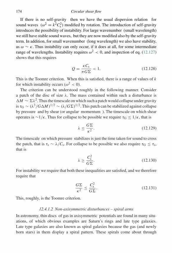
174 Circular shear flow
If there is no self-gravity then we have the usual dispersion relation forsound waves (ω2 = k2C2
s ) modified by rotation. The introduction of self-gravityintroduces the possibility of instability. For large wavenumber (small wavelength)we still have stable sound waves, but they are now modified also by the self-gravityterm. In addition, for small wavenumber (long wavelength) we also have stability,as ω ∼ κ . Thus instability can only occur, if it does at all, for some intermediaterange of wavelengths. Instability requires ω2 < 0, and inspection of eq. (12.127)shows that this requires
Q = κCs
πG�< 1. (12.128)
This is the Toomre criterion. When this is satisfied, there is a range of values of kfor which instability occurs (ω2 < 0).
The criterion can be understood roughly in the following manner. Considera patch of the disc of size λ. The mass contained within such a disturbance is�M ∼ �λ2. Thus the timescale on which such a patch would collapse under gravityis τG ∼ (λ3/G�M )1/2 ∼ (λ/G�)1/2. This patch can be stabilized against collapseby pressure and by shear (or angular momentum ). The timescale on which shearoperates is ∼1/κ . Thus for collapse to be possible we require τG ≤ 1/κ , that is
λ ≤ G�
κ2. (12.129)
The timescale on which pressure stabilizes is just the time taken for sound to crossthe patch, that is τs ∼ λ/Cs. For collapse to be possible we also require τG ≤ τs,that is
λ ≥ C2s
G�. (12.130)
For instability we require that both these inequalities are satisfied, and we thereforerequire that
G�
κ2≤ C2
s
G�. (12.131)
This, roughly, is the Toomre criterion.
12.4.1.2 Non-axisymmetric disturbances – spiral arms
In astronomy, thin discs of gas in axisymmetric potentials are found in many situ-ations, of which obvious examples are Saturn’s rings and late type galaxies.Late type galaxies are also known as spiral galaxies because the gas (and newlyborn stars) in them display a spiral pattern. These spirals come about through
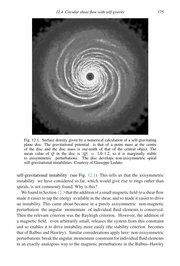
12.4 Circular shear flow with self-gravity 175
Fig. 12.1. Surface density given by a numerical calculation of a self-gravitatingplane disc. The gravitational potential is that of a point mass at the centreof the disc and the disc mass is one-tenth of that of the central object. Themean value of Q in the disc is 〈Q〉 = 1.0–1.2, so it is marginally stableto axisymmetric perturbations. The disc develops non-axisymmetric spiralself-gravitational instabilities. Courtesy of Giuseppe Lodato.
self-gravitational instability (see Fig. 12.1). This tells us that the axisymmetricinstability we have considered so far, which would give rise to rings rather thanspirals, is not commonly found. Why is this?
We found in Section 12.3 that the addition of a small magnetic field to a shear flowmade it easier to tap the energy available in the shear, and so made it easier to drivean instability. This came about because in a purely axisymmetric non-magneticperturbation the angular momentum of individual fluid elements is conserved.Then the relevant criterion was the Rayleigh criterion. However, the addition ofa magnetic field, even arbitrarily small, releases the system from this constraintand so enables it to drive instability more easily (the stability criterion becomesthat of Balbus and Hawley). Similar considerations apply here: non-axisymmetricperturbations break the angular momentum constraint for individual fluid elementsin an exactly analogous way to the magnetic perturbations in the Balbus–Hawley
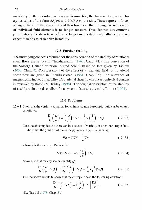
176 Circular shear flow
instability. If the perturbation is non-axisymmetric, the linearized equation foruφ has terms of the form ∂P/∂φ and ∂�/∂φ on the r.h.s. These represent forcesacting in the azimuthal direction, and therefore mean that the angular momentumof individual fluid elements is no longer constant. Thus, for non-axisymmetricperturbations the shear term (κ2) is no longer such a stabilizing influence, and weexpect it to be easier to drive instability.
12.5 Further reading
The underlying concepts required for the consideration of the stability of rotationalshear flows are set out in Chandrasekhar (1961, Chap. VII). The derivation ofthe Solberg–Høiland criterion sented here is based on that given by Tassoul(2000, Chap. 3). Considerations of the effect of a magnetic field on rotationalshear flow are given in Chandrasekhar (1961, Chap. IX). The relevance ofmagnetically induced instability of rotational shear flow in the astrophysical contextis reviewed by Balbus & Hawley (1998). The original description of the stabilityof a self-gravitating disc, albeit for a system of stars, is given by Toomre (1964).
12.6 Problems
12.6.1 Show that the vorticity equation for an inviscid non-barotropic fluid can be writtenas follows:
D
Dt
(ω
ρ
)=(
ω
ρ
)· ∇u − 1
ρ∇(
1
ρ
)∧ ∇p. (12.132)
Note that this implies that there can be a source of vorticity in a non-barotropic fluid.Show that the gradient of the enthalpy h = e + p/ρ is given by
∇h = T∇S + 1
ρ∇p, (12.133)
where S is the entropy. Deduce that
∇T ∧ ∇S = −∇(
1
ρ
)∧ ∇p. (12.134)
Show also that for any scalar quantity Q
D
Dt
(ω
ρ· ∇Q
)= D
Dt
(ω
ρ
)· ∇Q + ω
ρ· D
Dt[∇Q]. (12.135)
Use the above results to show that the entropy obeys the following equation:
D
Dt
(ω
ρ· ∇S
)=(
ω
ρ
)· ∇[
DS
Dt
]. (12.136)
(See Tassoul (1978, Chap. 3).)
12.6 Problems 177
12.6.2 Show that in axisymmetric motion, the specific angular momentum L = Ruφ =R2� of a fluid element remains constant as we follow its motion. Show that theradial (R) and axial (z) equations of motion can be written in a form replacing anyterms in uφ with a force L2/R3 acting in the radial direction.
An incompressible fluid with uniform density ρ is in cylindrical shear flow,with angular velocity �(R). Consider the exchange of two elementary annuli(rings) of fluid of equal heights and mass, caused by axisymmetric fluid motions.The rings are at R1 and R2 and have small radial extents dR1 and dR2 and massesdm = 2πρR1dR1 = 2πρR2dR2. Calculate the change in energy caused by theexchange of the rings and show how this is related to the Rayleigh stability criterion.
13
Modes in rotating stars
We have seen in earlier chapters that in a non-rotating star there are basicallytwo types of wave modes possible. The p-modes resemble sound waves as therestoring force in the oscillation comes from pressure. The g-modes resemblesurface water waves as their restoring force comes from gravity. In this chapterwe consider the new effects which can arise if the star is rotating. To do thiswe need a more sophisticated model for a star. Previously we took our ‘star’ aseither a horizontally stratified atmosphere or as a gas in a one-dimensional box.To consider rotational effects we need an axisymmetric base state. In line withour philosophy of keeping things as simple as possible, without jettisoning anyessential physics, we take as our model star a circular cylinder of incompressiblefluid. This eliminates the consideration of p-modes.
13.1 The non-rotating ‘star’
We start by considering the wave modes in the non-rotating ‘star’. In equilibriumthis is a cylinder of fluid of radius R0, with constant density ρ and pressure p(R),sitting in a gravitational potential �(R). The gravitational potential may be imposedfrom outside: it may result entirely from self-gravity of the cylinder, or it may bea mixture of the two. In equilibrium the velocity field is zero and the equation ofhydrostatic equilibrium yields
− 1
ρ
dp
dR− d�
dR= 0. (13.1)
Initially we consider waves with no z-dependence; that is, waves for which uz = 0and ∂/∂z = 0. Thus all we expect in this situation is waves travelling around thecurved surface of the cylinder in the azimuthal direction. In this case the linearized
178
13.1 The non-rotating ‘star’ 179
equations of motion are given by
∂uR
∂t= − 1
ρ
∂p′
∂R− ∂�′
∂R− ρ′
ρ
d�
dR(13.2)
and∂uφ
∂t= − 1
Rρ
∂p′
∂φ− 1
R
∂�′
∂φ. (13.3)
We emphasize that although the fluid is incompressible, so that δρ = 0, the Euleriandensity perturbation ρ′ is non-zero because the fluid surface is distorted by theperturbation. Thus if the radial component of the Lagrangian perturbation is ξR,the Eulerian density perturbation is given by
ρ′ = ρξRδ(R − R0). (13.4)
The linearized continuity equation is given by
1
R
∂
∂R(RuR) + 1
R
∂uφ
∂φ= 0, (13.5)
and the linearized version of Poisson’s equation is given by
∇2�′ = 4πGρ′. (13.6)
Using the symmetry of the unperturbed configuration, we can now Fourieranalyze in the usual way by taking all quantities to vary as∝ exp{i(ωt+mφ+kz)}. Inthis case we have assumed no z-dependence, so that k = 0. Making this substitution,and defining the quantity W by
W = p′
ρ+ �′, (13.7)
the above equations become
iωuR = −dW
dR− ρ′
ρ
d�
dR, (13.8)
iωuφ = imW
R, (13.9)
1
R
d
dR(RuR) + imuφ
R= 0 (13.10)
and1
R
d
dR
(R
d�′
dR
)− m2
R2�′ = 4πGρξRδ(R − R0). (13.11)
We eliminate uφ between eqs. (13.9) and (13.10) to obtain
iω
R
d
dR(RuR) = m2W
R2. (13.12)
180 Modes in rotating stars
Then using eq. (13.8) everywhere except at R = R0 (i.e. wherever ρ′ = 0)
iωuR = −dW
dR, (13.13)
we obtain an equation for W valid everywhere except at R = R0:
1
R
d
dR
(R
dW
dR
)− m2W
R2= 0. (13.14)
Inside the star, R < R0, the solution that is finite at the origin is given by
W (R) ∝ Rm, (13.15)
and we assume that m �= 0.Similarly, the solution of eq. (13.11) is straightforward except at R = R0.
Choosing the solutions which are finite at the origin and at infinity we find (form �= 0) that
�′ ={�′
0(R/R0)m, R < R0,
�′0(R/R0)
−m, R > R0.(13.16)
Here �′0 is the value of �′ at R = R0, and we have chosen the solutions so that �′
is continuous at R = R0. The value of �′0 is fixed by the jump in d�′/dR across
R = R0. Integrating eq. (13.11) across R = R0, we find that the jump is given by[d�′
dR
]+
−= 4πGξR. (13.17)
From this we obtain
�′0 = 2πGρR0
mξR, (13.18)
where the r.h.s. is to be evaluated at R = R0.We must now apply the free surface boundary condition at the surface of our
‘star’. This requires δp = 0 at R = R0, giving
limR→R0
(p′
ρ− ξRg
)= 0, (13.19)
where the surface gravity g = d�/dR, evaluated at R = R0, and g > 0.Alternatively we may write this as follows:
limR→R0
(W − �′ − ξRg) = 0. (13.20)
To put this in a more useful form, we use eq. (13.18) to write �′ in terms of ξR
and then use the relationship ur = iωξR together with eq. (13.13) to write ξR interms of dW/dR. Note that in doing this we have used the equations which arevalid for R �= R0, so that we have implicitly used the fact that limR→R0 ρ′ = 0,
13.2 Uniform rotation 181
even though the value of ρ′ there is formally infinite! The boundary condition nowbecomes
ω2W + dW
dR
[−g + 2πGρR0
m
]= 0, (13.21)
all to be evaluated at R = R0. Now from our solution for W given by eq. (13.15)we see that
limR→R0
1
W
dW
dR= m
R0. (13.22)
Hence we find the mode frequencies as follows:
ω2 = mg
R0− 2πGρ, (13.23)
provided m �= 0. Of course the mode m = 0 represents a simple radial expansionor contraction of the cylinder, and cannot occur for an incompressible fluid. Thesemodes correspond to surface gravity waves (g-modes).
13.1.1 Self-gravitating cylinder
If the cylinder is to be a proper model of a ‘star’, we must demand that theunperturbed gravitational potential � results solely from the gravity of the cylinderitself. Thus,
1
R
d
dR
(R
d�
dR
)= 4πGρ. (13.24)
From this we can show that the surface gravity g = d�/dR is given by
g = 2πGρR0. (13.25)
Thus the oscillation frequencies of a self-gravitating cylinder are given by
ω2 = (m − 1)g
R0. (13.26)
We note that although a mode with m = 1 is permitted, its frequency is zero.Since such a mode represents a simple translation of the star perpendicular to itsaxis of symmetry, this is exactly what we would expect. If you move a star bodilysideways, there is nothing to move it back.
13.2 Uniform rotation
We now consider the effect on the stellar modes of adding a small amount ofuniform rotation �. There are two basic effects, which we discuss in Sections 13.2.1and 13.2.2.
182 Modes in rotating stars
13.2.1 Effect on p- and g-modes
Rotation changes the equilibrium shape of the star by the addition of a centrifugalforce into the equation of hydrostatic equilibrium. But this gives a term of order∼ �2. Thus to first order in the rotation rate � the basic structure of the star, andtherefore its modes of oscillation, are not affected. However, there is a simplekinematic effect which is known as frequency splitting.
We found the azimuthal modes in the non-rotating cylinder to have the form
ξR ∝ sin(ωt) sin(mφ), (13.27)
or equivalentlyξR ∝ cos(ωt − mφ) − cos(ωt + mφ). (13.28)
We may view these as two surface waves, one moving in the positive φ-directionwith phase velocity ω/m and the other moving in the negative φ-direction withphase velocity −ω/m.
We have noted that the structure of a slowly rotating star is essentially unchanged.Therefore if we move with the rotating frame, the star is at rest and we can applythe analysis of the preceding section. The azimuthal coordinate φ′ in the rotatingframe is related to the azimuthal coordinate φ in the inertial frame by
φ′ = φ − �t. (13.29)
We conclude therefore that for a slowly rotating star the modes take the form
ξR ∝ cos(ωt − mφ′) − cos(ωt + mφ′), (13.30)
where the modal frequencies ω are unchanged to this order. Then in the inertial(non-rotating) frame the modes take the form
ξR ∝ cos[(ω + m�)t − mφ] − cos[(ω − m�)t + mφ]. (13.31)
Thus the effect of rotation is to split the frequency of the mode:
ω → ω ± m�. (13.32)
This is known as rotational splitting.
13.2.1.1 The Chandrasekhar –Friedmann–Schutz instability
The idea of rotational splitting leads to the remarkable conclusion that the emissionof gravitational waves makes all rotating stars unstable! Einstein’s general theoryof relativity predicts that gravitational waves are emitted when a time-dependentdensity distribution gives rise to a time-dependent gravitational field. Gravitationalwaves have a quadrupole or higher multipole character, so that only modes withm ≥ 2 produce them.
13.2 Uniform rotation 183
We consider the effect of gravitational wave emission on the modes we havebeen discussing.
First, we consider the non-rotating star. All the modes consist of two travellingwaves, each moving with angular speed ω/m, one moving in the positive φ-direction and the other in the negative φ-direction (see eq. (13.28)). The one movingin the positive φ-direction has a positive associated angular momentum. Thegravitational wave it emits also has positive angular momentum, so the effect ofgravitational wave emission is to reduce the amplitude of the wave and thus damp it.Exactly the same argument applies to the wave moving in the negative φ-direction.
Now consider what happens if the star is rotating. The wave which was movingin the positive φ-direction is still moving in that direction, but now (in the inertialframe) with angular speed ω/m + �. Thus it still emits a gravitational wave withpositive angular momentum, and therefore damps. But the wave which was movingin the negative φ-direction now has angular speed −ω/m + � in that direction.Thus if ω < m� this wave moves in the positive φ-direction in the inertial frame.If this happens, as it must for large enough m, then the wave, which has negativeassociated angular momentum, actually starts to emit gravitational radiation withpositive angular momentum. This means that the wave amplitude grows and is thebasis for what is called the Chandrasekhar–Friedmann–Schutz (CFS) instability.
In reality, damping processes occur fastest for the high-m modes, and thisinstability is not thought to operate for most stars. You can test this out by stampingon the ground (this should produce waves with m ∼ 109) and seeing what happens!However, the instability is thought to play a role in limiting the rotation rate forneutron stars. These are very compact stars, with escape velocities from theirsurfaces around 10–20 per cent of the speed of light. This means that when theyrotate rapidly, any surface features (such as waves) move at a speed v which isa significant fraction of the speed of light c and so become efficient emitters ofgravitational waves (the emitted energy goes as (v/c)6). Neutron stars can reachvery rapid rotation rates by accreting matter with the Keplerian angular momentumat their equators. This gravitational wave instability would ultimately limit theirspin rates if nothing else does at slower spin rates, and this is probably the reasonthat they appear to show a maximum rotation period of around 1.5 ms.
13.2.2 The r-modes
The second effect of introducing rotation is to give rise to a completely new set ofmodes, the rotational modes, or r-modes. Consider a perturbation of the form
ξ = (0, ξφ(R, z), 0). (13.33)
184 Modes in rotating stars
If the star is not rotating, then all this perturbation does is displace azimuthal ringsof material in the φ-direction. Since the star is axi-symmetric, the equilibrium isunchanged and there is no restoring force which tries to put the fluid rings backwhere they were. In other words, the frequency associated with such a perturbationis ω = 0. But if the star (or, in our case, cylinder) is rotating, then this displacementchanges the angular velocity of the ring. This upsets the equilibrium of the star(which comes about through a balance between gravity, pressure gradient andcentrifugal force) and so gives rise to oscillations. As we shall see, a typicalfrequency of the oscillations can be expected to be ω ∼ �.
We return to eqs. (12.28) and (12.29) which we derived in Chapter 12. We assumeall variables go as ∝ exp{i(ωt + mφ + kz)}. In Chapter 12 we defined the Rayleighdiscriminant, which for the uniform rotation we consider here is given by
R = 4�2, (13.34)
and we defined the Doppler-shifted frequency,
σ = ω + m�. (13.35)
We note that for uniform rotation, σ is independent of radius R. Then, in terms ofthe variables W = p′/ρ and ξR, the linearized equations are given by
1
R
d
dR(RξR) − 2mω
σRξR = 1
σ 2
(m2
R2+ k2
)W (13.36)
and
[σ 2 − 4�2]ξR = dW
dR+ 2m�
σRW . (13.37)
We can now eliminate ξR between these two equations to get a second-orderordinary differential equation for W :
d2W
dR2+ 1
R
dW
dR−[(
1 − 4�2
σ 2
)k2 + m2
R2
]W = 0. (13.38)
For a non-rotating incompressible cylinder, the only possible wave modes aresurface waves (g-modes). To eliminate these we impose the boundary conditionthat ξR = 0 at the surface of the cylinder R = R0. From eq. (13.37) we see that, interms of W , this implies
dW
dR+ 2m�
σRW = 0 (13.39)
at R = R0.We consider first what happens if the modes are independent of z, i.e. if k = 0.
Without loss of generality, we may take m ≥ 0. Then for m �= 0 the solution whichis finite at R = 0 is
W ∝ Rm. (13.40)
13.2 Uniform rotation 185
Since for this solution W and dW/dR have the same sign, we cannot now satisfy theboundary condition, eq. (13.39). For m = 0 the solution that is finite at the originis of the form W = const. and corresponds to uniform radial expansion, whichcannot occur for an incompressible fluid. We conclude that the r-modes must allhave z-dependence.
We now need to recall briefly the basic properties of Bessel functions. Thisshould not come as a surprise as they are the natural functions for describingoscillations in cylindrical geometry. The standard version of Bessel’s equationfor y(x) is as follows:
d2y
dx2+ 1
x
dy
dx+(
α2 − ν2
x2
)y = 0. (13.41)
This has two independent solutions, which are oscillatory. These are Jν(αx), whichis the cylindrical equivalent of sin x and (for ν �= 0) is zero at x = 0, and Yν(αx),which is the cylindrical equivalent of cos x and is singular at x = 0. The modifiedversion of Bessel’s equation (obtained by the transformation x → ix) is as follows:
d2y
dx2+ 1
x
dy
dx−(
α2 + ν2
x2
)y = 0. (13.42)
This has two independent solutions which are non-oscillatory – the modified Besselfunctions. These are Iν(αx), which (for ν �= 0) is zero at x = 0 and is the cylindricalequivalent of exp x, and Kν(αx), which is singular at x = 0 and is the cylindricalequivalent of exp(−x).
Returning to eq. (13.38), we see that if σ 2 > 4�2 then the solution which is finiteat x = 0 has the form W ∝ Im(αR) for some real α. But in this case W and dW/dRhave the same sign, and we cannot then satisfy the boundary condition given ineq. (13.39). This tells us that the r-mode frequencies must satisfy σ 2 < 4�2, i.e.
−2� < σ < 2�. (13.43)
When this is satisfied, we can define the real number α by
α =[
4�2
σ 2− 1
]1/2
> 0. (13.44)
Then the solution to eq. (13.38) is given by
W = Jm(αkR). (13.45)
Substituting this solution into the boundary condition, eq. (13.39), gives
αkJ ′m(αkR0) + 2m�
σRJm(αkR0) = 0, (13.46)
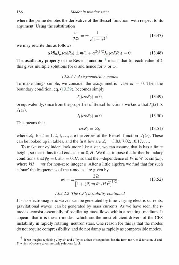
186 Modes in rotating stars
where the prime denotes the derivative of the Bessel function with respect to itsargument. Using the substitution
σ
2�= ± 1√
1 + α2, (13.47)
we may rewrite this as follows:
αkR0J ′m(αkR0) ± m(1 + α2)1/2Jm(αKR0) = 0. (13.48)
The oscillatory property of the Bessel function † means that for each value of kthis gives multiple solutions for α and hence for σ or ω.
13.2.2.1 Axisymmetric r-modes
To make things simple, we consider the axisymmetric case m = 0. Then theboundary condition, eq. (13.39), becomes simply
J ′0(αkR0) = 0, (13.49)
or equivalently, since from the properties of Bessel functions we know that J ′0(x) ∝
J1(x),J1(αkR0) = 0. (13.50)
This means thatαkR0 = Zi, (13.51)
where Zi, for i = 1, 2, 3, . . ., are the zeroes of the Bessel function J1(z). Thesecan be looked up in tables, and the first few are Zi = 3.83, 7.02, 10.17, . . ..
To make our cylinder look more like a star, we can assume that is has a finiteheight, so that it has fixed ends at z = 0, H . We then impose the further boundaryconditions that ξR = 0 at z = 0, H , so that the z-dependence of W is W ∝ sin(kz),where kH = nπ for non-zero integer n. After a little algebra we find that for sucha ‘star’ the frequencies of the r-modes are given by
ωi = ± 2�[1 + (ZinπR0/H )2]1/2
. (13.52)
13.2.2.2 The CFS instability continued
Just as electromagnetic waves can be generated by time-varying electric currents,gravitational waves can be generated by mass currents. As we have seen, the r-modes consist essentially of oscillating mass flows within a rotating medium. Itappears that it is these r-modes which are the most efficient drivers of the CFSinstability in rapidly rotating neutron stars. One reason for this is that the modesdo not require compressibility and do not damp as rapidly as compressible modes.
† If we imagine replacing J by sin and J ′ by cos, then this equation has the form tan A = B for some A andB, which of course gives multiple solutions for A.
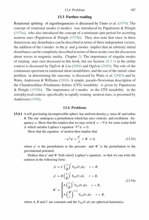
13.4 Problems 187
13.3 Further reading
Rotational splitting of eigenfrequencies is discussed by Unno et al. (1979). Theconcept of rotational modes (r-modes) was introduced by Papaloizou & Pringle(1978a), who also introduced the concept of a minimum spin period for accretingneutron stars (Papaloizou & Pringle (1978b). They also note that since in threedimensions any disturbance can be described in terms of three independent vectors,the addition of the r-modes to the p- and g-modes implies that an arbitrary initialdisturbance can be completely described in terms of these modes (see the discussionabout waves in magnetic media, Chapter 2). The importance of singular modesof rotating stars (not discussed in this book, but see Section 10.3.1) in the stellarcontext is discussed by Ogilvie & Lin (2004) and Ogilvie (2005). The role of thecontinuous spectrum in rotational shear instabilities, and the use of the initial-valueproblem in determining the outcome, is discussed by Watts et al. (2003) and byWatts, Andersson & Williams (2004). A simple, pseudo-Newtonian description ofthe Chandrasekhar–Friedmann–Schutz (CFS) instability is given by Papaloizou& Pringle (1978b). The importance of r-modes in the CFS instability in theastrophysical context, specifically in rapidly rotating neutron stars, is presented byAndersson (1998).
13.4 Problems
13.4.1 A self-gravitating incompressible sphere has uniform density ρ, mass M and radiusR. The star undergoes a perturbation which has zero vorticity and oscillation fre-quency ω. Show that this implies that we may write ξ = −∇ψ for some scalar fieldψ which satisfies Laplace’s equation ∇2ψ = 0.
Show that the equation of motion then implies that
−ω2ψ + p′
ρ+ �′ = 0, (13.53)
where p′ is the perturbation to the pressure and �′ is the perturbation to thegravitational potential.
Deduce that p′ and �′ both satisfy Laplace’s equation, so that we can write thesolution in the following form:
ψ = C( r
R
)lYlm(θ , φ), r < R,
p′ = B( r
R
)lYlm(θ , φ), r < R,
�′ =
⎧⎪⎪⎨⎪⎪⎩
A( r
R
)lYlm(θ , φ), r < R,
A
(R
r
)l+1
Ylm(θ , φ), r > R,
(13.54)
where A, B and C are constants and the Ylm(θ , φ) are spherical harmonics.
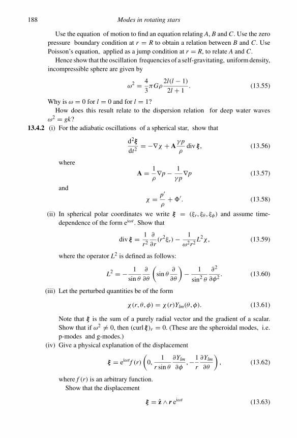
188 Modes in rotating stars
Use the equation of motion to find an equation relating A, B and C. Use the zeropressure boundary condition at r = R to obtain a relation between B and C. UsePoisson’s equation, applied as a jump condition at r = R, to relate A and C.
Hence show that the oscillation frequencies of a self-gravitating, uniform density,incompressible sphere are given by
ω2 = 4
3πGρ
2l(l − 1)
2l + 1. (13.55)
Why is ω = 0 for l = 0 and for l = 1?How does this result relate to the dispersion relation for deep water waves
ω2 = gk?13.4.2 (i) For the adiabatic oscillations of a spherical star, show that
d2ξ
dt2= −∇χ + A
γ p
ρdiv ξ , (13.56)
where
A = 1
ρ∇p − 1
γ p∇p (13.57)
and
χ = p′
ρ+ �′. (13.58)
(ii) In spherical polar coordinates we write ξ = (ξr , ξθ , ξφ) and assume time-dependence of the form eiωt . Show that
div ξ = 1
r2
∂
∂r(r2ξr) − 1
ω2r2L2χ , (13.59)
where the operator L2 is defined as follows:
L2 = − 1
sin θ
∂
∂θ
(sin θ
∂
∂θ
)− 1
sin2 θ
∂2
∂φ2. (13.60)
(iii) Let the perturbed quantities be of the form
χ(r, θ , φ) = χ(r)Ylm(θ , φ). (13.61)
Note that ξ is the sum of a purely radial vector and the gradient of a scalar.Show that if ω2 �= 0, then (curl ξ)r = 0. (These are the spheroidal modes, i.e.p-modes and g-modes.)
(iv) Give a physical explanation of the displacement
ξ = eiωt f (r)
(0,
1
r sin θ
∂Ylm
∂φ, −1
r
∂Ylm
∂θ
), (13.62)
where f (r) is an arbitrary function.Show that the displacement
ξ = z ∧ r eiωt (13.63)
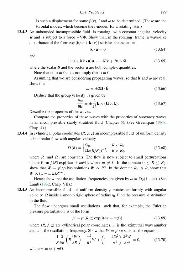
13.4 Problems 189
is such a displacment for some f (r), l and ω to be determined. (These are thetoroidal modes, which become the r-modes for a rotating star.)
13.4.3 An unbounded incompressible fluid is rotating with constant angular velocity� and is subject to a force −∇�. Show that, in the rotating frame, a wave-likedisturbance of the form exp{i(ωt + k · r)} satisfies the equations
k · u = 0 (13.64)
andiωu + i(k · u)u = −iBk + 2u ∧ �, (13.65)
where the scalar B and the vector u are both complex quantities.Note that u · u = 0 does not imply that u = 0.Assuming that we are considering propagating waves, so that k and ω are real,
show thatω = ±2� · k. (13.66)
Deduce that the group velocity is given by∂ω
∂k= ± 2
k3k ∧ (� ∧ k). (13.67)
Describe the properties of the waves.Compare the properties of these waves with the properties of buoyancy waves
in an incompressible stably stratified fluid (Chapter 5). (See Greenspan (1968,Chap. 4).)
13.4.4 In cylindrical polar coodinates (R, φ, z) an incompressible fluid of uniform densityis in circular flow with angular velocity
�(R) ={�0, R < R0,�0(R/R0)
−2, R > R0,(13.68)
where R0 and �0 are constants. The flow is now subject to small perturbationsof the form f (R) exp{i(ωt + mφ)}, where m �= 0. In the domain 0 ≤ R ≤ R0,show that W = p′/ρ has solutions W ∝ Rm. In the domain R0 ≤ R, show thatW ∝ (ω + m�)R−m.
Hence show that the oscillation frequencies are given by ω = �0(1 − m). (SeeLamb (1932, Chap. VII).)
13.4.5 An incompressible fluid of uniform density ρ rotates uniformly with angularvelocity � inside a smooth rigid sphere of radius r0. Find the pressure distributionin the fluid.
The flow undergoes small oscillations such that, for example, the Eulerianpressure perturbation is of the form
p′ = p′(R, z) exp{i(ωt + mφ)}, (13.69)
where (R, φ, z) are cylindrical polar coordinates, m is the azimuthal wavenumberand ω is the oscillation frequency. Show that W = p′/ρ satisfies the equation
1
R
∂
∂R
(R
∂W
∂R
)− m2
R2W +
(1 − 4�2
σ 2
)∂2W
∂z2= 0, (13.70)
where σ = ω + m�.
190 Modes in rotating stars
Derive the boundary condition satisfied by W on the sphere R2 + z2 = r20 .
Show that there is an axisymmetric oscillation mode of the form
W = z(AR2 + Bz2 + C), (13.71)
where A, B and C are constants, with oscillation frequency given by
ω = ±√
5
2�. (13.72)
14
Cylindrical shear flow–non-axisymmetric instability
In several astrophysical contexts, notably in the study of accretion discs, we wouldlike to know whether certain types of rotating shear flow are stable. If so, theseare potential candidates for realistic models of accretion flows. In Chapter 12 weconsidered cylindrical shear flow in an incompressible fluid. We showed that inthe absence of magnetic fields the flow is unstable to axisymmetric instability ifthe specific angular momentum is a decreasing function of radius – the Rayleighcriterion. Thus we need to ask if the converse is true; that is, whether stability isguaranteed if the Rayleigh criterion is satisfied.
We shall show here, by considering a particular example, that this converse isnot true. If non-axisymmetric perturbations are allowed, instability is still possibleeven if the Rayleigh criterion is satisfied.
14.1 Equilibrium configuration
We consider a cylindrical flow of an incompressible fluid with no z-dependence ina fixed gravitational potential:
�(R) = −GM
R. (14.1)
Note that this is a purely artificial potential, since R is the cylindrical radius notthe spherical radius r which appears in the gravitational potential � = −GM /rfor a point mass M at the origin. Since there is no z-dependence, the equilibriumequation is simply
− 1
ρ∇p − ∇� + R�2R = 0. (14.2)
Here �(R) is the angular velocity of the fluid. Replacing the centrifugal forceterm by a rotational potential of the form ��(R), where
∂��
∂R= −R�2, (14.3)
191
192 Cylindrical shear flow–non-axisymmetric instability
we can integrate the equilibrium equation to give
p
ρ+ � + �� = C, (14.4)
where C is a constant.We now specialize the flow to one for which the Rayleigh criterion is neutrally
satisfied, i.e. one for which R(R) = 0. Thus we have
�(R) = �0
(R0
R
)2
, (14.5)
where �0 is the angular velocity at some reference radius R0, yet to be defined.We note that in eq. (14.2) the gravitational force has the form FG ∝ −1/R2 and thecentrifugal force obeys F� ∝ 1/R3. This means that at small radii the centrifugalforce dominates and the net force is outwards, while at large radii the gravitationalforce dominates and the net force is inwards. Therefore at some radius, which wedefine as the reference radius R0, these two balance and we have FG + F� = 0.Using this definition we find that
R0�20 = GM
R20
, (14.6)
and hence that we can rewrite eq. (14.4) in the following form:
p(R)
ρ= C + GM
R− GMR0
2R2. (14.7)
For a given value of the constant C, this defines the distribution of pressure p(R).We note that by definition we have ensured that dp/dR = 0 at R = R0, and indeedp(R) reaches a maximum value of
pmax = ρ
(C + GM
2R0
)(14.8)
at that radius. For R > R0, p(R) is a monotonically decreasing function of R,reaching the value of p∞ = ρC in the limit as R → ∞. From eq. (14.7) we seethat, as R decreases, p(R) always becomes negative at some finite radius. Since inthe body of the fluid the pressure must always be positive, this implies that thefluid must have a cylindrical cavity surrounding the z = 0 axis.
We are interested here in finite configurations, which do not reach to infinity.This means that we require C < 0, so that there is no pressure at infinity. Also,for the configuration to exist at all, we require that pmax > 0. We shall thereforeredefine C in terms of a dimensionless parameter λ as follows:
C = −GM
λR0, (14.9)
14.2 The perturbation equations 193
where, for a finite fluid configuration, we now require 2 < λ < ∞. To locate theboundaries of the fluid configuration, we look for the radii at which p(R) = 0.Substituting all this into eq. (14.7) we find that the fluid configuration is in theregion R− ≤ R ≤ R+, where R± are the roots of a quadratic equation given by
R±R0
= 1
2(λ ±√
λ(λ − 2)). (14.10)
We note that we may define R− < R0 and R+ > R0. As λ → 2, the two rootsbecome almost equal and the fluid configuration is a slender cylindrical shell. Asλ → ∞, we see that R− → 1/2 while R+ → ∞.
Finally, for later use, we note that the effective gravity in the flow, g = ∇p/ρ,can be written as follows:
g(R) = GM
R20
[R0
R
]3 [1 − R
R0
]. (14.11)
Then of course at the inner radius, R = R−, the gravity g(R−) = g− > 0 actsradially outwards, while at the outer radius, R = R+, the gravity g(R+) = g+ < 0acts radially inwards.
14.2 The perturbation equations
We proceed exactly as before to obtain the linearized equations of motion, notingthat in this case we assume that there is no z-dependence. We also ignore the self-gravity of the fluid, so we assume the potential to be fixed, and note that the Euleriandensity perturbation ρ′ is zero everywhere except for a δ-function contribution atthe boundaries. As before, we take all quantities to vary as ∝ exp{i(ωt + mφ)} anddefine the Doppler-shifted frequency
σ(R) = ω + m�(R). (14.12)
Then in terms of the radial Lagrangian displacement ξR and the quantity W = p′/ρ,and recalling that here � ∝ 1/R2, eqs. (12.28) and (12.29) become
σ 2(
dξR
dR+ ξR
R
)− 2m�σ
RξR = m2
R2W (14.13)
and
σ 2ξR = dW
dR+ 2m�
σRW . (14.14)
Because � ∝ 1/R2, these equations can be simplified by using the substitution
W = σH . (14.15)
194 Cylindrical shear flow–non-axisymmetric instability
Then eq. (14.14) becomes simply
σξR = dH
dR, (14.16)
and eq. (14.13) becomes
d
dR(σξR) + σ
ξR
R= m2
R2H . (14.17)
Eliminating ξR from these two equations, we obtain
1
R
d
dR
(R
dH
dR
)− m2
R2H = 0. (14.18)
This is a second-order equation for H with eigenvalues ω, once we have appliedappropriate boundary conditions. We know from Chapter 4 that if we have fixedboundaries ξR = 0 there are no surface waves (the incompressible equivalent ofp- and g-modes). In addition, since we have no z-dependence, then there are nointernal waves (r-modes). Thus, in order to allow something to happen we must letthe boundaries move. The simplest boundary condition, and the most appropriateone from an astrophysical point of view, is to allow free boundaries at R = R±.Thus at R = R± we let
δp = p′ + ξRdp
dR= 0. (14.19)
This implies that
W + gξR = 0, (14.20)
which, in turn, using the definition of H and eq. (14.16), gives
σ 2H + gdH
dR= 0, (14.21)
which is valid at R = R±.The general solution to eq. (14.18) is as follows:
H = C1Rm + C2R−m, (14.22)
where C1 and C2 are constants. Applying the boundary condition, eq. (14.21), atR = R− and R = R+, and then eliminating the constants C1 and C2, we obtain theeigenvalue equation for ω:
(ω + m�−)2 + mg−/R−(ω + m�+)2 + mg+/R+
=(
R+R−
)2m(ω + m�−)2 − mg−/R−(ω + m�+)2 − mg+/R+
, (14.23)
where we have written �± = �(R±). This is a quartic equation for ω.
14.3 The Papaloizou–Pringle instability 195
14.3 The Papaloizou–Pringle instability
The roots of the quartic equation,eq. (14.23), are able to give rise to unstable growingmodes, i.e. values of ω such that Im(ω) < 0. This happens for the following reason.At the inner edge there are two sets of waves, travelling relative to the fluid in thepositive and negative φ-directions. The same applies at the outer edge. However,because � ∝ 1/R2, the fluid at the inner edge is moving at an angular velocity �−greater than the angular velocity �+ at the outer edge. The instability occurs whena wave which is travelling backwards relative to the fluid at the inner edge has thesame angular phase speed as a wave which is travelling forwards relative to the fluidat the outer edge. When this happens the waves can communicate and exchangeangular momentum and energy . The situation here is exactly analogous to theone we discussed in Chapter 13 regarding the Chandrasekhar –Friedmann–Schutzinstability. The wave at the inner edge transfers angular momentum outwardsto the wave at the outer edge. The wave at the outer edge has positive angularmomentum and is gaining angular momentum so it grows in amplitude. Thewave at the inner edge which is losing angular momentum is a wave of negativeangular momentum, and so it too grows in amplitude. This signifies an instability,here called the Papaloizou–Pringle (PP) instability.
Here we consider two limiting cases, amenable to simple analysis, one stableand the other unstable.
14.3.1 Large m
Here we consider what happens in the limit of large m. In this limit the wavelengthsof the surface waves (2πR±/m in the azimuthal direction) become very short. Thusthey behave like deep-water waves and have frequencies (in the frame of the fluid)given by ω2 = mg±/R±. In eq. (14.23), the term (R+/R−)2m becomes very large inthe limit of large m and dominates all the other terms. For equality to hold therefore,we require either that the denominator of the l.h.s. or the numerator of the r.h.s.vanish. These two conditions, recalling that g+ < 0 and g− > 0, give the four rootsof the quadratic:
ω = −m�+ ±√m|g+|/R+, (14.24)
which correspond to the expected surface waves on the outer edge, and
ω = −m�− ±√mg−/R−, (14.25)
which correspond to surface waves on the inner edge. For such surface waves, thephase velocities are ∝ 1/
√m so there is no chance of the backward wave at the
inner surface being in phase with the forward wave on the outer surface. Thus in thislimit the waves are stable. Moreover at such large values of m, the depth to which
196 Cylindrical shear flow–non-axisymmetric instability
such waves propagate means that the waves on the two surfaces do not interact andmove independently.
14.3.2 Thin cylindrical shell
We consider the limit λ → 2, so that the fluid is confined to a thin cylindrical shell.We do this at a fixed value of m and this now gives the waves a chance to interact.Thus we set
λ = 2(1 + ε2) (14.26)
and consider the limit ε � 1. To first order in ε, we find that
R± = R0(1 ± ε), (14.27)
thatg± = ±εR0�
20 (14.28)
and that�± = �0(1 ∓ 2ε). (14.29)
It is convenient to defineσ0 = ω + m�0, (14.30)
so thatω + m�± = ω + m�0 ∓ 2m�0ε. (14.31)
Substituting this into eq. (14.23) and keeping only first-order terms in ε, the equationreduces to
σ 2 = −2�20. (14.32)
This impliesω = −m�0 ± i�0
√2. (14.33)
We note two things about this result. First, the real part of the eigenfrequency issuch that the eigenmode co-rotates with the fluid at radius R = R0. It is essentialthat unstable modes co-rotate with the fluid at some radius, so that forward andbackward travelling waves have a chance to interact. We already found that thiswas a requirement for instability in the linear shear flow (Chapter 10). Second,the growth rate of the instability is dynamical, with the growth timescale being oforder the rotation period of the fluid. Thus, even though according to the Rayleighcriterion the fluid is on the margin of stability to axisymmetric modes, it isactually dynamically unstable to non-axisymmetric modes. This demonstrates thedistinction between local and global instability. The Rayleigh criterion is purelylocal, whereas the PP instability explicitly involves the conditions at the inner andouter boundaries of the flow. In astrophysical applications the PP instability showsthat the possible forms of rotating shear flows in accretion discs are severelyrestricted.
14.5 Problems 197
14.4 Further reading
The original description of the Papaloizou–Pringle instability is to be found inPapaloizou & Pringle (1984). The simplified analysis presented here is based onBlaes & Glatzel (1986).
14.5 Problems
14.5.1 A torus of non-self-gravitating polytropic fluid (index n) rotates about the R = 0axis with uniform specific angular momentum h and is subject to the gravitationalfield of a point mass M at the origin R = z = 0. Show that the structure of the torusis given by
(n + 1)p
ρ= GM
R0
⎡⎣(
R20
R2 + z2
)1/2
− 1
2
(R0
R
)2
− C
⎤⎦ , (14.34)
where C is a constant and the density maximum is at R = R0, z = 0, whereh2 = GMR0.
Describe approximately the shapes of the tori for values of C in the range 0 <
C < 1/2. If C ≈ 1/2 show that the torus is very slender and has a nearly circularcross section. (See Papaloizou & Pringle (1984).)
14.5.2 Consider the torus discussed in Problem 14.5.1. Show that small perturbations ofthe form ∝ exp{i(ωt + mφ)} obey the equation
1
R
∂
∂R
(ρR
∂W
∂R
)= −m2
R2ρW + ∂
∂z
(ρ
∂W
∂z
)= −σ 2ρ2
γ pW , (14.35)
where W = p′/ρσ and σ = ω + m�.14.5.3 An infinite cylinder (0 ≤ R ≤ R0) of incompressible fluid with uniform density ρ0
rotates about the axis R = 0 with velocity u0 = (0, R�(R), 0), with �(R) = kR,where k is a constant.
The fluid is self-gravitating. Show that if the central pressure p(R=0) =π2G2ρ3
0/k2, then the radius is R0 = (2πGρ0)1/2/k and the effective surface gravity
is zero.The fluid is subject to small perturbations so that, for example, the velocity is
u0 + u, where u is of the form
u ∝ (uR(R), uφ(R), 0) exp{i(ωt + mφ)}. (14.36)
Show that the perturbation equations are given by
iσuR − 2�uφ = −dW
dR, (14.37)
3�uR + iσuφ = − im
RW (14.38)
198 Cylindrical shear flow–non-axisymmetric instability
andduR
dR+ uR
R+ im
Ruφ = 0, (14.39)
where σ = ω + m�(R) and W = p′/ρ + �′.Show that these equations can be reduced to the following single equation:
d2uR
dR2+ 3
R
duR
dR+{
1 − m2 − 3m�
σ
}uR
R2= 0. (14.40)
Now consider the case m = 1. Show that a solution to this equation is given by
uR = 1 + kR
ω. (14.41)
Assuming that this is the only solution which is regular at R = 0, show that theoscillation frequencies obey the equation ω2 = 0. Give a physical explanation ofthis result.
In this case the solution given is apparently singular. Find the solution toeq. (14.40) for the case m = 1 and ω = 0, which is regular at the origin, andcomment on how it is obtained from the solution given in the limit ω → 0. (SeeWatts et al. (2003, 2004), and also refer to Balbinski (1984).)
References
Andersson, N. (1998).Anew class of unstable modes of rotating relativistic stars, Astrophys.J., 502, 708.
Balbinski, E. (1984). The continuous spectrum in differentially rotating perfect fluids: amodel with an analytic solution, Mon. Not. Royal Astron. Soc., 209, 145.
Balbus, S. A. & Hawley, J. F. (1998). Instability, turbulence, and enhanced transport inaccretion disks, Rev. Mod. Phys., 70, 1.
Batchelor, G. K. (1967). An Introduction to Fluid Dynamics (Cambridge: CambridgeUniversity Press).
Billingham, J. & King, A. C. (2000). Wave Motion (Cambridge: Cambridge UniversityPress).
Blaes, O. M. & Glatzel, W. (1986). On the stability of incompressible constant angularmomentum cylinders, Mon. Not. Royal Astron. Soc., 220, 253.
Blandford, R. D. & Rees, M. J. (1974). A ‘twin-exhaust’ model for double radio sources,Mon. Not. Royal Astron. Soc., 169, 395.
Bondi, H. (1952). On spherically symmetrical accretion, Mon. Not. Royal Astron. Soc.,112, 195.
Chandrasekhar, S. (1961). Hydrodynamic and Hydromagnetic Stability (Oxford: OxfordUniversity Press); republished in 1981 by Dover Publications, Inc., New York.
Clayton, D. D. (1983). Principles of Stellar Evolution and Nucleosynthesis (Chicago:University of Chicago Press).
Coles, P. & Lucchin. (1995). Cosmology – The Origin and Evolution of Cosmic Structure(New York: John Wiley & Sons).
Cox, J. P. (1980). Theory of Stellar Pulsation (Princeton: Princeton University Press).Doroshkevich, A. G. (1980). Fragmentation of a primordial flat layer, and the formation of
internal cluster structure, Soviet Astronomy, 24, 152.Drazin, P. & Reid, W. (1981). Hydrodynamic Stability (Cambridge: Cambridge University
Press).Elphick, C., Regev, O. & Shaviv, N. (1992). Dynamics of fronts in thermally bistable fluids,
Astrophys. J., 392, 106.Elphick, C., Regev, O. & Spiegel, E. A. (1991). Complexity from thermal instability, Mon.
Not. Royal Astron. Soc., 250, 617.Field, G. B. (1965). Thermal instability, Astrophys. J., 142, 531.Field, G. B., Rather, J. D. G., Aannenstad, P. A. & Orszag, S. A. (1968). Hydromagnetic
shock waves and their infrared emission in HI regions, Astrophys. J., 151, 953.Garaud, P. (2002). On rotationally driven meridional flows in stars, Mon. Not. Royal Astron.
Soc., 335, 707.Gerwin, R. A. (1968). Stability of the interface between two fluids in relative motion, Rev.
Mod. Phys., 40, 652.Greenspan, H. P. (1968). The Theory of Rotating Fluids (Cambridge: Cambridge University
Press).
199
200 References
Howard, L. N. (1961). Note on a paper of John W. Miles, J. Fluid Mech., 10, 509.Jackson, J. D. (1998). Classical Electrodynamics, 3rd edn (New York: John Wiley & Sons,
Inc.).Jeans, Sir J. H. (1929). Astronomy and Cosmogony, 2nd edn (Cambridge: Cambridge
University Press); republished in 1961 by Dover Publications, Inc., New York.Königl, A. (1982). On the nature of bipolar sources in dense molecular clouds, Astrophys.
J., 261, 115.Lamb, Sir H. (1932). Hydrodynamics, 6th edn (Cambridge: Cambridge University Press);
republished in 1945 by Dover Publications, Inc., New York.Landau, L. D. & Lifshitz, E. M. (1959). Fluid Mechanics (Oxford: Pergamon Press).Ledoux, P. (1951). Sur la stabilité gravitationelle d’une nébuleuse isotherme, Ann.
Astrophys., 14, 438.Lifshitz, E. M. & Pitaevskii, L. P. (1980). Statistical Physics, 3rd edn, part 1 (Oxford:
Pergamon Press).Lubow, S. H. & Pringle, J. E. (1993). The gravitational stability of a compressed slab of
gas, Mon. Not. Royal Astron. Soc., 263, 701.Meerson, B. (1996). Non-linear dynamics of radiative condensations in optically thin
plasmas, Rev. Mod. Phys., 68, 215.Miles, J. W. (1961). On the stability of heterogeneous shear flows, J. Fluid Mech., 10, 496.Ogilvie, G. I. & Lin, D. N. C. (2004). Tidal dissipation in rotating giant planets, Astrophys.
J., 610, 477.Ogilvie, G. I. (2005). Wave attractors and the asymptotic dissipation rate of tidal
disturbances, J. Fluid Mech., 543, 16.Papaloizou, J. & Pringle, J. E. (1978a). Non-radial oscillations of rotating stars and their
relevance to the short period oscillations of cataclysmic variables, Mon. Not. Royal Astron.Soc., 182, 423.
Papaloizou, J. & Pringle, J. E. (1978b). Gravitational radiation and the stability of rotatingstars, Mon. Not. Royal Astron. Soc., 184, 501.
Papaloizou, J. & Pringle, J. E. (1984). The dynamical stability of differentially rotatingdiscs with constant specific angular momentum, Mon. Not. Royal Astron. Soc., 208, 721.
Parker, E. N. (1979). Cosmical Magnetic Fields – Their Origin and Their Activity (Oxford:Clarendon Press).
Pringle, J. E. & Rees, M. J. (1972).Accretion disc models for compact x-ray sources, Astron.Astrophys., 21, 1.
Roberts, P. H. (1967). An Introduction to Magnetohydrodynamics (London: Longmans,Green and Co. Ltd).
Sedov, L. (1959). Similarity and Dimensional Methods in Mechanics (New York: AcademicPress).
Shu, F. H. (1992). Gas Dynamics (Millvalley, CA: University Science Books).Sturrock, P. A. (1994). Plasma Physics – An Introduction to the Theory of Astrophysical,
Geophysical and Laboratory Plasmas (Cambridge: Cambridge University Press).Tassoul, J.-L. (1978). Theory of Rotating Stars (Princeton: Princeton University Press).Tassoul, J.-L. (2000). Stellar Rotation (Cambridge: Cambridge University Press).Taylor, G. I., (1959a). The formation of a blast wave by a very intense explosion. II. The
atomic explosion of 1945, Proc. Roy. Soc. London A, 201, 159.Taylor, G. I., (1959b). The formation of a blast wave by a very intense explosion. I.
Theoretical discussion, Proc. Roy. Soc. London A, 201, 175.Toomre, A. (1964). On the gravitational stability of a disk of stars, Astrophys. J., 139,
(1217).Turner, J. S. (1973). Buoyancy Effects in Fluids (Cambridge: Cambridge University Press).
References 201
Unno, W., Osaki, Y., Ando, H. & Shibahashi, H. (1979). Non-Radial Oscillations of Stars(Tokyo: University of Tokyo Press).
Watts, A. L., Andersson, N. & Williams, R. L. (2004). The oscillation and stability ofdifferentially rotating spherical shells: the initial-value problem, Mon. Not. Royal Astron.Soc., 350, 927.
Watts, A. L., Andersson, N., Beyer, H. & Schutz, B. F. (2003). The oscillation and stabilityof differentially rotating spherical shells: the normal-mode problem, Mon. Not. RoyalAstron. Soc., 342, 1156.
Weinberg, S. (1972). Gravitation and Cosmology – Principles and Applications of theGeneral Theory of Relativity (New York: John Wiley & Sons, Inc.).
Witham, G. B. (1974). Linear and Non-Linear Waves (New York: John Wiley & Sons).Zel’dovich, Ya. B. & Novikov, I. D. (1971). In K. S. Thorne & W. D. Arnett, Relativistic
Astrophysics, Vol. 1: Stars and Relativity (Chicago: University of Chicago Press).Zel’dovich, Ya. B. & Raizer, Yu. P. (1967). Physics of Shockwaves and High-Temperature
Hydrodynamic Phenomena (New York: Academic Press).

Index
accretion, 45, 47, 49, 50, 58, 158, 171, 191, 196accretion discs, 125, 171, 174, 191, 196acoustic waves, 19, 21, 22, 24, 25, 86, 103, 109,
116, 124, 130, 134, 145adiabatic flow, 7, 8advection, 11, 12, 156
of magnetic field, 12of vortex lines, 11, 12, 16
Alfvén velocity, 22, 39Alfvén waves, 24angular frequency, 21atmosphere, 16, 48, 50, 57, 62, 85–88, 97–100,
102, 107–110, 178plane-parallel, 78, 79, 87, 88polytropic, 84, 88, 98
axisymmetric flow, 150, 162, 172axisymmetric instability, 175, 191axisymmetric perturbations, 161, 165, 167,
171, 175axisymmetric r-modes, 186, 194axisymmetric stability, 196axisymmetric stability of an incompressible
rotating fluid, 162
barotropic fluid, 11, 15, 151, 152, 154, 157, 176Bernoulli constant, 47Bernoulli equation, 11, 45Bernoulli theorem, 35Bessel equation, 185Bessel function, 86, 87, 185, 186
modified, 185blast wave, Taylor-Sedov solution, 57Bondi, 46–50, 58Bondi accretion, 45, 46, 50, 58, 59Bondi radius, 49, 50boundary conditions, 47, 48, 56, 62, 87, 105,
112, 122, 136, 137, 144, 148, 162,186, 194
Brunt–Väisälä frequency, 79buoyancy, 78, 84–86, 102, 107, 127, 144, 145
magnetic, 102, 109
Cepheid, 90Chandrasekhar, 77, 111, 112, 145, 148, 171,
176, 182, 195Chandrasekhar–Friedmann–Schutz instability,
182, 195characteristic curves, 28–30, 32charge density, 10circular shear flow, 158, 162
with a magnetic field, 167with self-gravity, 172
compressibility, 111, 145, 186compressible media, 17–43conductivity, 1, 10, 92–94, 97, 98, 100, 103,
113, 116–121electrical, 6thermal, 6, 92, 100, 113, 119–121
conservationof angular momentum, 16, 150of energy, 5, 6, 12, 13of entropy, 7, 26of magnetic flux, 37of mass, 2of momentum, 3, 4, 41, 45, 52, 134
convection, 62, 73, 74, 98, 107, 110, 156instability, 74, 90, 163Schwarzschild criterion, 74, 79, 85, 107, 162,
165, 167cooling, 2, 113–118, 120, 121
of astrophysical gases, 113, 114slow, 116, 117
cooling front, 120cooling function, 114, 115
d’Alembert’s principle, 164damping, 90, 93–95, 97, 101, 183diffusivity, 15
magnetic, 15dispersion relation, 20–23, 82–84, 89, 106,
108–110, 116, 120, 124, 130, 131, 146,170, 173, 174, 188
displacement current, 9divergence theorem, 3, 33, 34, 36
203
204 Index
Eddington–Sweet circulation, 155eigenfunction, 70, 87, 94, 95, 99, 100, 137eigenvalue, 56, 70, 87, 89, 94, 99, 120, 137,
161, 162, 170, 194electric charge density, 4electric current, 186electric field, 4, 10energy, 5–7, 12–14energy density, 13, 14, 41, 152energy density equation, 12–14energy flux, 14, 61energy generation, 7, 14, 61, 62, 96, 101, 152energy input, 51, 56energy internal, 5, 6, 35, 76, 91, 92, 163energy kinetic, 6, 13, 14, 35, 57, 71, 76, 88,
108, 163energy loss, 134energy magnetic, 6, 13, 14, 76, 106, 108, 109energy nuclear, 6, 95, 96, 152energy production, 61, 95–97enthalpy, 176entropy, 5, 7, 8, 19, 35, 40, 54, 67, 74, 85, 102,
162–164, 176equation of motion, 4equation of state, 6–7equation of continuity, 165, 169, 179Eulerian, perturbation, 18, 19, 38, 64–67, 75,
80, 160, 164, 179, 189, 193Eulerian vs. Lagrangian, 63evanescent, 79, 137exchange of stabilities, 70, 127explosion, 38, 50, 51, 53, 57, 58
in uniform medium, 50supernova, 38, 50, 57
fast/slow magnetosonic waves, 25, 39Ferraro’s law of isorotation, 156field lines, magnetic, 12, 16, 24, 25, 36, 38, 59,
110, 156, 157, 169flow
barotropic, 8compressible, 17, 26, 162isentropic, 8, 45non-linear, 26, 38spherically symmetric, 44, 50, 58, 60
steady inflow, 44steady outflow, 50
of traffic, 38fluid
definition of, 1, 2magnetic, 36
forceelectric, 4electromagnetic, 10
pressure, 26, 46Fourier transform, 20, 22, 68, 79, 80, 94, 104,
108, 135, 138, 142frequency
epicyclic, 173rotational splitting, 182, 187
frequency wave, 21
g-mode, 79, 83, 84, 89, 103, 178, 181, 182, 184,187, 188, 194
galaxy, 44gas
compressible, 29, 30, 120perfect, 6–8, 20, 40, 41, 54, 56, 62, 96, 98,
115, 121, 152gas law, 20, 40, 41gravitational collapse, 124, 150gravitational field, 76, 88, 103, 106, 111, 142,
144–146, 162, 182, 197gravitational force, 3, 131, 162, 172, 192gravitational potential, 3
effective, 152gravitational radiation, 182, 183, 186group velocity, 21, 23, 38, 84, 189
heat, 5–8, 35, 38, 61, 93, 94, 97, 99, 100, 103,113, 152–155
conduction of, 5, 14, 19, 61, 93generation of, 6
heating/cooling front, 117hydromagnetic shock, 41
incompressible flow, 15, 17induction equation, 10, 22, 104, 107, 147,
156, 168initial-value problem, 29, 138, 187instability, 135, 175
Balbus–Hawley, 171, 175, 176buoyancy, 102, 106Chandrasekhar–Friedmann–Schutz, 183,
186, 187epsilon mechanism, 95–97Field criterion, 114, 117, 118gravitational, 123, 129, 130, 175Hertzsprung–Russell diagram, 90, 101Jeans, 123–125kappa mechanism, 97, 98of linear shear flow, 196magnetic buoyancy, 106MRI (magnetorotational), 171Papaloizou–Pringle, 187, 195, 197Parker, 102, 107, 108Rayleigh criterion, 196
Index 205
incompressible flow (contd.)Richardson criterion, 144Schwarzschild criterion, 73of self-gravitating fluid, 150shear, 141Solberg–Høiland criterion, 162, 165, 176of stratified fluid, 162strip, 90, 101thermal, 113of thin slab, 129Toomre, 172, 174, 176
internal energy, 35inviscid fluid, 171isothermal gas, 130
Jeans criterion, 97, 101Jeans instability, 123–125Jeans length, 124, 128–130Jeans mass, 124jump conditions, 34, 36, 41, 51
Kelvin–Helmholtz instability, 155Kelvin–Helmholtz timescale, 155, 174Kelvin’s circulation theorm, 15kinetic energy density, 13Knudsen number, 2
Lagrangian derivative, 4, 5, 65, 119Lagrangian displacement, 64, 105, 160, 193Lagrangian perturbation, 18, 66, 86, 103, 105,
142, 168, 179Lagrangian vs. Eulerian, 18, 38, 63–66, 74Lamb wave, 83Laplace equation, 104, 105, 187Laplace transform, 138Legendre equation, 128Legendre polynomials, 128Liapunov functional, 121linear perturbations, 114linear shear flow, 134
bounded, 148stratified, 142, 144
linear wave equation, 19local analysis, 82, 170Lorentz force, 10Lorentz transformation of fields, 9
Mach number, 35, 40, 42, 52magnetic energy density, 13magnetic field, 3, 8–14magnetorotational instability (MRI), 171
magnetohydrodynamics (MHD) approximation,8–10, 12–14, 17, 24, 33, 35, 36
magnetohydrodynamic equation, 26, 41magnetosonic waves, 24, 25mass conservation equation, 2, 3Maxwell equation, 9, 10, 13, 157
displacement current, 9Maxwell stress tensor, 3, 4mean free path, 1, 2, 4, 6, 31, 33, 37meridional circulation, 154, 155, 157MHD, see magnetohydrodynamics, 8, 14, 15modes
g-modes, 79, 83, 84, 89, 103, 178, 181, 182,184, 187, 188, 194
normal, 4, 33, 34p-modes, 78, 84, 86, 178, 188in rotating stars, 178of self-gravitating incompressible cylinder,
181, 184of self-gravitating incompressible sphere, 187spheroidal, 188
non-axisymmetric disturbances, 174non-axisymmetric instability, 191non-axisymmetric perturbations, 176, 191nozzle, subsonic/supersonic flow transition, 29,
42, 50, 58, 118, 119, 134
Ohm’s Law, 9, 10opacity, 61, 62, 97, 100, 152orthogonality, 87, 100oscillation, 78–83, 86–88, 90–97, 99–101, 178,
181, 184, 185, 187–190, 198damping, 100
by conduction, 154, 155excitation, 90, 93, 97, 101, 113
the epsilon mechanism, 96the kappa mechanism, 97
hanging chain, 86stellar, 21, 62, 63, 78, 83, 87, 93, 97, 101
oscillation mode, 97, 99, 190overstability, 97
p-mode, 78, 84, 86, 178, 188perfect gas law, 56, 62, 91, 98, 103perturbation
adiabatic, 20, 66, 67, 75, 129, 166Eulerian, 99, 123, 142, 143irrotational, 21Lagrangian, 63–65, 67, 68
phase velocity, 21, 39, 84, 142, 144, 182piston, 31, 32, 37, 42Poisson’s equation, 3, 61, 75, 123, 126, 127,
129, 153, 173, 179, 188
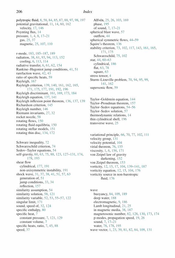
206 Index
polytropic fluid, 8, 58, 84, 85, 87, 88, 97, 98, 197potential gravitational, 11, 14, 60, 162
velocity, 17, 146Poynting flux, 14pressure, 1, 4, 8, 17–21
gas, 25, 37magnetic, 25, 107, 110
r-mode, 183, 185–187, 189radiation, 38, 61, 93, 94, 113, 152
cooling, 6, 113, 114radiative transfer, 6, 61, 62, 154Rankine–Hugoniot jump conditions, 41, 51rarefaction wave, 42, 43ratio of specific heats, 59Rayleigh, 167Rayleigh criterion, 139, 140, 161, 162, 165,
171, 175, 177, 191, 192, 196Rayleigh discriminant, 161, 169, 173, 184Rayleigh equation, 137, 141Rayleigh inflexion point theorem, 136, 137, 139Richardson criterion, 145Rayleigh number, 146Riemann invariants, 27, 32rocket nozzle, 58rotating flows, 150rotating fluid equilibria, 150rotating stellar models, 151rotating thin disc, 134, 172
Schwarz inequality, 72Schwarzschild criterion, 74Sedov–Taylor equations, 54self-gravity, 60, 63, 75, 88, 123, 127–131, 174,
178, 193shear flow
cylindrical, 177, 191non-axisymmetric instability, 191
shock wave, 31, 37, 38, 41, 51, 57, 63generation of, 51jump conditions, 33, 34reflection, 157
similarity assumption, 54similarity solution, 58, 121similarity variable, 52, 53, 55–57, 122singular limit, 171sound, speed of, 32, 124specific enthalpy, 80specific heat, 7
constant pressure, 7, 121, 129constant volume, 7
specific heats, ratio, 7, 45, 88speed, 37
Alfvén, 25, 26, 103, 169phase, 195of sound, 7, 17–21
spherical blast wave, 57outflow, 44
spherical symmetric flows, 44–59Squire’s theorem, 136stability criterion, 73, 102, 117, 143, 161, 165,
171, 175Schwarzschild, 75, 102
star, 44, 60–63cylindrical, 186flat, 63, 78square, 63
stress tensor, 4Sturm–Liouville problem, 70, 94, 95, 99,
141, 162supersonic flow, 59
Taylor–Goldstein equation, 144Taylor–Proudman theorem, 157Taylor–Sedov equations, 54–56Taylor–Sedov solution, 57thermodynamic relations, 14thin cylindrical shell, 196transverse wave, 25
variational principle, 66, 70, 77, 102, 111velocity group, 131velocity potential, 104virial theorem, 76, 155viscosity, 1, 6, 156, 171von Zeipel law of gravity
darkening, 152von Zeipel theorem, 153vorticity, 12, 15, 17, 104, 139–141, 187vorticity equation, 12, 15, 104, 176vorticity source in non-barotropic
fluid, 176
wavebuoyancy, 84, 109, 189deep water, 188electromagnetic, 9, 186Lamb longitudinal, 21, 25in magnetic media, 38, 187magnetosonic number, 82, 128, 130, 173, 174p-modes, propagation speed, 19, 26sound, 7, 17–21water, 78, 178, 195
wave vector, 1, 23, 39, 81, 82, 84, 109, 131