+ All Categories
Home > Documents > PRIORITIZING LEVEE IMPROVEMENTS A Thesis Submitted to …

PRIORITIZING LEVEE IMPROVEMENTS A Thesis Submitted to …

Date post: 24-Feb-2022
Category:
Upload: others
View: 1 times
Download: 0 times
Share this document with a friend
75
PRIORITIZING LEVEE IMPROVEMENTS A Thesis Submitted to the Faculty of Purdue University by Brian J Meunier In Partial Fulfillment of the Requirements for the Degree of Master of Science in Civil Engineering December 2011 Purdue University West Lafayette, Indiana
Transcript

PRIORITIZING LEVEE IMPROVEMENTS

A Thesis

Submitted to the Faculty

of

Purdue University

by

Brian J Meunier

In Partial Fulfillment of the

Requirements for the Degree

of

Master of Science in Civil Engineering

December 2011

Purdue University

West Lafayette, Indiana

ii

TABLE OF CONTENTS

Page

LIST OF TABLES .......................................................................................................................... iv

LIST OF FIGURES.......................................................................................................................... v

ABSTRACT ..................................................................................................................................vii

CHAPTER 1 INTRODUCTION ........................................................................................................ 1

CHAPTER 2 STUDY AREA BACKGROUND INFORMATION .............................................................. 4

2.1 Indianapolis Flood Control Infrastructure ..................................................................... 5

2.2 Study Reaches ............................................................................................................. 6

2.2.1 Urban Levee System: WR-C1 and HD-C1 .............................................................. 6

2.2.2 Rural Levee System: WR-02, WR-03, and Unnamed Levee ................................... 7

CHAPTER 3 STUDY AREA LEVEE PRIORITIZATION METHODOLOGY ............................................... 9

3.1 Hydrologic Model Development .................................................................................. 9

3.1.1 Watershed and Stream Network Delineation ..................................................... 10

3.1.2 Curve Number Development ............................................................................. 11

3.1.3 Rainfall Simulation and Model Calibration.......................................................... 11

3.2 Hydraulic Model Development .................................................................................. 12

3.2.1 Channel Geometry ............................................................................................. 12

3.2.2 Initial and Boundary Conditions ......................................................................... 13

3.2.3 Levee Breaching ................................................................................................. 14

3.2.4 Unsteady-Flow Simulation ................................................................................. 15

3.3 Breach Damage Estimation ........................................................................................ 15

3.4 Improvement Cost Assessment .................................................................................. 16

CHAPTER 4 STUDY AREA RESULTS ............................................................................................. 18

4.1 Hydraulic Results for Levee Breaches ......................................................................... 18

4.1.1 Storage Area Stage and Flow Hydrograph Analysis ............................................. 18

4.1.2 Inundation Areas and Depth Grids ..................................................................... 25

iii

Page

4.2 Breach Damage Estimation Data ................................................................................ 31

4.3 Improvement Cost Data ............................................................................................. 31

CHAPTER 5 CONCLUSIONS ........................................................................................................ 33

5.1 Unsteady-flow Modeling............................................................................................ 33

5.2 Storage Areas ............................................................................................................ 34

5.3 Priority Ratio ............................................................................................................. 35

5.4 Decision Guidance and Project Justification ............................................................... 36

CHAPTER 6 TOPICS FOR FUTURE DEVELOPMENT ....................................................................... 37

6.1 Loss-of-life Modeling ................................................................................................. 37

6.2 Social and Cultural Impacts of Flooding ...................................................................... 37

6.3 Environmental Benefits of a Natural Floodplain ......................................................... 38

6.4 Engineered Levee Breaches ....................................................................................... 38

6.5 Levee Breach Progression .......................................................................................... 39

WORKS CITED ........................................................................................................................... 40

APPENDICES .............................................................................................................................. 42

Appendix A – Flood of Record: 1913 ...................................................................................... 42

Appendix B - Hydrologic Modeling Data & Results ................................................................. 44

Appendix C – Hydraulic Modeling Results .............................................................................. 48

Appendix D – Breach Damage Estimation .............................................................................. 50

Appendix E – Improvement Cost Estimates ........................................................................... 51

Appendix F – Levee Prioritization Statistics ............................................................................ 56

Appendix G – Further Considerations .................................................................................... 59

iv

LIST OF TABLES

Table Page

Table 1: Curve Number Matrix .................................................................................................. 11

Table 2: Manning Roughness Ranges for Study Areas ................................................................ 13

Table 3: IDNR Suggested Breach Parameters ............................................................................. 14

Table 4: Modeled Levee Breach Parameters .............................................................................. 15

Table 5: Requirements of 44 CFR 65.10 ..................................................................................... 16

Table 6: Levee Breach and Storage Area Results ........................................................................ 18

Table 7: Breach Equalization Time and Stage Loss Results ......................................................... 25

Table 8: Breach Loss Summary .................................................................................................. 31

Table 9: Improvement Cost Summary ....................................................................................... 32

Table 10: Comparison of Unsteady and Steady-flow Flood Elevations ....................................... 34

Appendix Table

Table B.1: Hydrologic Parameter Summary ............................................................................... 45

Table D 1: Summary of HAZUS Breach Loss Estimation .............................................................. 50

Table F.1: Priority Ratio vs. Hydraulic Statistics .......................................................................... 56

Table F.2: Priority Ratio vs. Zoning Statistics .............................................................................. 56

Table F.3: Priority Ratio vs. Social Statistics ............................................................................... 57

Table F.4: Priority Ratio vs. Breach Loss Statistics ...................................................................... 57

Table F.5: Priority Ratio vs. Improvement Cost Statistics ........................................................... 58

v

LIST OF FIGURES

Page

Figure 1: Study Area Location Map .............................................................................................. 5

Figure 2: Urban Levee Study Area Located in Washington Township, Indianapolis, IN ................. 7

Figure 3: Rural Levee Study Area Located in Perry Township, Indianapolis, IN ............................ 8

Figure 4: Combined Study Area Watershed and Stream Network .............................................. 10

Figure 5: Typical Levee Cross-section ........................................................................................ 17

Figure 6: WR-C1 Stage and Flow Hydrographs ........................................................................... 19

Figure 7: HD-C1 Stage and Flow Hydrographs ............................................................................ 20

Figure 8: UNL Stage and Flow Hydrographs ............................................................................... 22

Figure 9: WR-02 Stage and Flow Hydrographs ........................................................................... 23

Figure 10: WR-03 Stage and Flow Hydrographs ......................................................................... 24

Figure 11: WR-C1 Levee Breach Depth Grid ............................................................................... 26

Figure 12: HD-C1 Levee Breach Depth Grid ............................................................................... 27

Figure 13: UNL Levee Breach Depth Grid ................................................................................... 28

Figure 14: WR-02 Levee Breach Depth Grid ............................................................................... 29

Figure 15: WR-03 Levee Breach Depth Grid ............................................................................... 30

Appendix Figure

Figure B.1: Observed Peak Annual Streamflow vs. Log-Pearson Type III Distribution ................. 44

Figure B.2: Stream Length vs. Contributing Watershed Area...................................................... 44

Figure B.3: Watershed Areas and Ground Surface Elevation ...................................................... 45

Figure B.4: WFK White River Streamflow Hydrograph at 82nd Street Bridge ............................. 46

Figure B.5: Howland Ditch Streamflow Hydrograph at confluence with WFK White River .......... 46

Figure B.6: WFK White River Streamflow Hydrograph at Southport Road Bridge ....................... 47

Figure C.1: Unsteady-flow vs. Steady-state Floodplain Boundaries for HD-C1 Levee Breach....... 48

vii

ABSTRACT

Meunier, Brian J. M.S.C.E., Purdue University, December 2011. Prioritizing Levee Improvements. Major Professor: Venkatesh Merwade. Levees exist all over the United States, which protect land and property from devastating floods.

Many of these levees are more than half of a century old, and were initially intended to serve as

protection for farmland; however, increases in development and urban sprawl have caused a

rise in the number of homes being sheltered by levees that were not designed with the

necessary level of protection. A lack of inclusive record keeping and inspection has left many

levees in dire need of costly repairs. This study attempts to define a practical and economical

means of prioritizing levee repairs based on the economic risk posed by the breaching of

impaired levees and the expected improvement costs for returning the levees to a safer

condition. A framework for a simplified breach damage analysis is proposed through a case

study of five levees in a flood-prone area in central Indiana. Current analysis methods are

examined and compared to the proposed methodology.

Results of the case study provide a means of analytically prioritizing levee repairs, reveal pitfalls

of the current standards of practice, and identify future research needs for advancement of the

prioritization procedure. The use of an unsteady-flow analysis with storage areas to represent

the protected areas is identified as a key component to a realistic characterization of the

physical system. Comparisons between breach results, economic costs, and characteristics of

the protected areas reveal no apparent correlations, suggesting a need for a ranking parameter.

A Priority Ratio is identified in the case study results and suggested for use.

1

CHAPTER 1 INTRODUCTION

Catastrophes have thrust the topic of flood control infrastructure into the national spotlight in

the recent years. Levees in New Orleans were breached during Hurricane Katrina, leaving

citizens homeless, bereaved, and helpless in 2005. Midwestern America became a national

disaster site in the summer of 2008 as levees and dams were damaged and destroyed by

relentless, widespread rainfall.

Levees exist all over the United States, which protect land and property from devastating floods.

These levees provide a vital service in the form of preservation of human life as well as

maintaining the value of the homes that lie in the protected area. Critical components of

infrastructure and industrial sites are also often located adjacent to streams and rivers due a

reliance on connectivity to a large source of water, requiring levees to prevent crippling damage

to the facilities.

Though this infrastructure goes unnoticed or unrecognized by much of the population,

approximately 43 percent of the United States population lives in one of the 692 counties that

contain levees. The United States Army Corps of Engineers (USACE) estimates that some

100,000 miles of levee exist in the United States. The vast majority, around 86 percent, is locally

owned and maintained (USACE, 2006). Local ownership and maintenance has allowed the

condition of private levees to remain unknown by governing bodies. Many of these levees are

more than half of a century old and were initially intended to serve as protection for farmland;

however, increases in development and urban sprawl have caused a rise in the number of

homes being sheltered by levees that were not designed with the necessary level of protection.

Many Americans are unaware of the dangers of living in flood protected areas. The absence of

mandatory flood insurance seems to convey a sense of safety, or lack of risk; however, surveys

of the flood protection infrastructure of the United States have revealed serious flaws in this

rationale (USACE, 2006).

2

A lack of inclusive record keeping and inspection has left many levees in dire need of repairs. As

of 2009, only 10 states retained any listing of the levees within their borders. Perhaps more

shockingly, a mere 23 states have a form of oversight on levee safety. (ASCE, 2009) The

combination of these two factors can allow for the unchecked degradation of these critical

components of infrastructure. USACE’s current inventory of federally inspected levees states

that 9% of the 1,967 levees listed are expected to fail during a significant flooding event (ASCE,

2009). The increased development density behind levees, coupled with declining levee

conditions has the potential for devastating loss of human life, destruction of personal and

public property, as well as severe damage to other important infrastructure. Levee failures

resulting from Hurricane Katrina and the Midwest Flood in 2005 and 2008, respectively, led to

1,834 deaths and an estimated economic damage of more than $200 billion (NCLS, 2009). These

levee failures can result from deficient levees; however, the failures can also stem from

inadequate design. After the adoption of the National Flood Insurance Program in 1968, many

levees were designed to provide adequate protection for the 1% annual chance flooding event

to exclude the owners in the protected areas from having to purchase flood insurance. Though

the 1% annual chance flood was never intended for use as design criteria (NCLS, 2009), the

economical incentives to construct levees to the minimum elevations required to eliminate

mandatory flood insurance have forced a Spartan approach to levee construction.

In recognition of the pitfalls in levee safety and oversight, the National Committee on Levee

Safety (NCLS) has issued evaluations of the current system. America’s levee infrastructure was

given a “D-“ in the American Society of Civil Engineers’ “Report Card for America’s

Infrastructure,” citing that the potential for loss cannot be overlooked (ASCE, 2009). In 2009,

the NCLS submitted a report to Congress with numerous recommendations for a National Levee

Safety Program. Among the recommendations listed was the establishment of a hazard

potential classification system (NCLS, 2009). A set of criteria used for a more holistic assessment

of risk, beyond the probability of occurrence, have yet to be formally developed.

The overabundance of levees existing in poor condition creates an economic issue, in addition to

the obvious safety concerns. It is not feasible, nor practical, for all levees to be repaired and

upgraded to meet the requirements set forth in the National Flood Insurance Program under

3

Title 44 Code of Federal Regulation 65.10 (44 CFR 65.10). The extent of the deficient structures

as well as the expense involved in rehabilitating flood control infrastructure will simply not allow

the repair of all structures. As a result, it is necessary to determine which levees to upgrade and

maintain in a responsible manner. Currently, there is no generally accepted method for

prioritizing levee repair or method for determining which levees should receive no additional

attention.

This study attempts to define a practical and economical means of prioritizing levee repairs

based on the economic risk posed by the breaching of impaired levees and the expected

improvement costs for returning the levees to a safer condition. A framework for a simplified

breach damage analysis is proposed through a case study of five levees in a flood-prone area in

central Indiana. Suggestions for advancement of the proposed method as well as future

research needs are explored.

4

CHAPTER 2 STUDY AREA BACKGROUND INFORMATION

In the United States, the topic of flooding is most often associated with the Mississippi River and

coastal regions subject to hurricane seasons. Flooding is not secluded to these regions. The

state of Indiana may not be the first place that comes to many Americans’ minds when they

think of flooding; however, Indiana has a long history of devastating floods. Even in more recent

times, catastrophic floods have created disaster areas out of much of the state. Since 2006,

there have been six flooding events severe enough for the government to declare affected areas

as federal disaster area. Ninety percent of Indiana’s 92 counties were declared federal disaster

areas in 2005 after heavy rainfall occurred in saturated watersheds. A total of $7 million in flood

insurance claims were paid. Extended periods of significant rainfall culminated in a massive

flood in June 2008. Rainfall exceeding the 1%-annual-chance event swept across the state

leading to over $175 million of federal disaster assistance (FEMA, 2011). After inspecting the

flooding history of Indiana, it is clear that the hazard of flooding is significant; however, the

exposure to flooding is equally significant. There are approximately 32,500 flood insurance

policies in effect statewide in Indiana, with approximately 22,000 of those policies covering

properties in high risk areas (FEMA, 2011). The majority of all major floods within Indiana occur

within the White, Wabash, and Ohio River basins. These rivers are relatively low energy rivers,

which must swell greatly to convey large amounts of runoff.

5

The two sites examined in this study are located in Indianapolis, Indiana; a study area location

map is shown in Figure 1. Indianapolis is split in half by the West Fork (WFK) White River and

has a significant amount of flood control infrastructure to combat the frequent high stages of

the river. Indianapolis, much like the rest of the state, is no stranger to flooding.

Figure 1: Study Area Location Map

2.1 Indianapolis Flood Control Infrastructure

As a result of previous floods and the obvious exposure to flood hazards, Indianapolis has

developed an extensive network of levees and floodwalls to protect itself from the rising waters

of the WFK White River and its tributaries. Extensive flood reduction and protection projects

began to be constructed in the 1920’s, continuing through the 1960’s. Reservoirs, major

diversions, and detention basins were built to increase storage, and to reduce peak channel flow

rates. Earthen levees and floodwalls were also constructed to reduce the remaining risk of

flooding (Bodenhamer & Barrows, 1994). The levees protect urban and rural areas in and

around the city. Nearly 39 miles of levees exist in the city and surrounding areas in a system of

48 levees; however, the Federal Emergency Management Agency (FEMA) only recognizes 32 of

the levees, a total of 29 miles, as providing the 1%-annual-chance level of flood protection. As

many of the levees were initially constructed nearly 100 years, the integrity of the structures has

6

deteriorated over time leaving them in a poor condition. Inspections performed by engineering

consultants suggest that 13 of the levees are in poor condition and are in need of significant

repairs (CBBEL, 2007). Based on the findings of the study, the flood control infrastructure of

Indianapolis is showing evidence of significant aging.

2.2 Study Reaches

Two reaches of the WFK White River were selected to serve as study areas. The levees selected

are different with respect to type of protection; one study area is primarily urban, while the

other study area is dominated by agriculture. The urbanized area has a clear need for flood

protection based on the number and types of structures being protected by the levee system.

The agriculturally based levee system serves as protection for some households and other

structures; however, the majority of the land area encompassed by the levee is open space or

farm fields. Finally, the levee systems differ in the apparent necessity for repairs based on a

visual inspection of deficiencies. The differing conditions of the protected areas and levee

conditions are desirable to convey the variability that may be expected in results and the

potential uses for the results of the analysis. In this instance, one would expect a levee that is

mildly deficient to be assessed a higher priority status than a levee that is significantly more

impaired if the former levee protected a much more populated area. The highly deficient levee

with a lower apparent value in terms of protected structures and property was selected to

display the need to consider abandonment of levees as opposed to rehabilitation. The areas

chosen also afford the opportunity to analyze several levee differing in length, height, and

flooding source. A more thorough description of each levee segment follows.

2.2.1 Urban Levee System: WR-C1 and HD-C1

The urban levee system analyzed in this study is slightly north of Broad Ripple Village, a cultural

district in the north-central portion of Indianapolis, Indiana. The area is primarily residential and

serves as home to one school. A small amount of commercial development also exists in the

area. The contributing watershed has a total area of 3,027 square kilometers (km2) and is

primarily agricultural, with 75.0% of the land being used for that purpose. Of the remaining

area, 18.3% is urbanized, 5.3% is forested, and 1.4% covered by open water (USGS, 2010). The

protected area is exposed to flood hazards from two different sources, WFK White River and

7

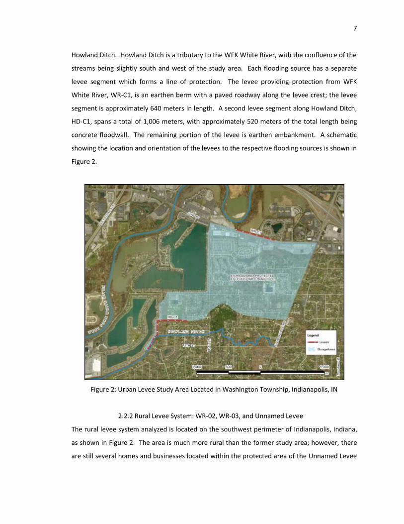
Howland Ditch. Howland Ditch is a tributary to the WFK White River, with the confluence of the

streams being slightly south and west of the study area. Each flooding source has a separate

levee segment which forms a line of protection. The levee providing protection from WFK

White River, WR-C1, is an earthen berm with a paved roadway along the levee crest; the levee

segment is approximately 640 meters in length. A second levee segment along Howland Ditch,

HD-C1, spans a total of 1,006 meters, with approximately 520 meters of the total length being

concrete floodwall. The remaining portion of the levee is earthen embankment. A schematic

showing the location and orientation of the levees to the respective flooding sources is shown in

Figure 2.

Figure 2: Urban Levee Study Area Located in Washington Township, Indianapolis, IN

2.2.2 Rural Levee System: WR-02, WR-03, and Unnamed Levee

The rural levee system analyzed is located on the southwest perimeter of Indianapolis, Indiana,

as shown in Figure 2. The area is much more rural than the former study area; however, there

are still several homes and businesses located within the protected area of the Unnamed Levee

8

(UNL). Levees WR-02 and WR-03 provide protection for a much smaller area which includes a

very small number of buildings and a portion of a golf course. The contributing watershed has a

total area of 4,885 km2 and is also primarily agricultural, with 65.0% of the land being used for

that purpose. Of the remaining area, 27.7% is urbanized, 5.6% is forested, and 1.6% covered by

open water (USGS, 2010). The sole flooding source is WFK White River; WR-02 and WR-03

reside on the west bank of the river and UNL is to the immediate east of the river. All levee

segments consist entirely of earthen berm. WR-02 runs along the west bank of the river for

approximately 920 meters; WR-03 is slightly north of WR-02 and is nearly 1,000 meters in

length. At nearly 21,000 meters in length, UNL is the longest levee. A schematic showing the

location and orientation of the levees is shown in Figure 3.

Figure 3: Rural Levee Study Area Located in Perry Township, Indianapolis, IN

9

CHAPTER 3 STUDY AREA LEVEE PRIORITIZATION METHODOLOGY

3.1 Hydrologic Model Development

Hydrologic models were developed for the urban and rural study reaches using standard

hydrologic engineering practices and the United States Army Corps of Engineers’ (USACE) HEC-

GeoHMS software add-in for ArcGIS. Publicly available data sources were used for all study area

datasets. Elevation data was gathered from the United States Geological Survey (USGS) from

the Seamless Server (USGS, 2010). A Digital Elevation Model (DEM) having a resolution of one-

third arc-second was downloaded for the region which would encompass both the urban and

rural study areas. Land use information was also taken from the USGS Seamless Server; the

National Land Cover Dataset grid had a cell size of one arc-second (USGS, 2006). Hydrologic soil

properties were taken from the 1:24000 SSURGO dataset made available by the Natural

Resource Conservation Service (NRCS, formerly the Soil Conservation Service, or SCS) (NRCS,

2010). Design rainfall data was collected from a National Oceanic and Atmospheric

Administration (NOAA) Atlas 14 frequency estimate near the centroid of the delineated

watershed. Each step in the hydrologic model development is discussed below.

10

3.1.1 Watershed and Stream Network Delineation

The contributing watersheds and stream networks were delineated for each study area. Once

the extent of the entire watershed contributing to the study areas was determined, the stream

network was based off of a threshold value of 4% determined by plotting the total stream

network length versus the defining watershed area percentage; a plot of stream length versus

contributing drainage area is shown in Appendix B. An additional stream branch was created to

include Howland Ditch in the stream network delineation. The entire stream network

developed for the study areas is shown in Figure 4. Subbasin boundaries were generated based

on the stream network delineation, resulting in a total of 17 subbasins. The subbasin

representing the drainage area for Howland Ditch was the smallest at 27.5 km2; the largest

subbasin was 827.2 km2. Times of concentration were determined by using the longest spatial

flowpath within each subbasin.

Figure 4: Combined Study Area Watershed and Stream Network

11

3.1.2 Curve Number Development

Runoff losses were modeled by using the SCS Curve Number Method. Soil type and land use

grids were spatially joined to determine the runoff generating capability of each subbasin within

the watershed. Hydrologic soil types were classified as A, B, C, or D, with all missing values

being assigned hydrologic soil type B. Land use classifications were reclassified into four bins:

water, medium residential, forest, and agricultural. Curve Numbers were then defined as

suggested by Table 1.

Table 1: Curve Number Matrix (McCuen, 1998)

Gridcode Land Use Description

Hydrologic Soil Type

A B C D

1 Water 100 100 100 100

2 Medium Residential 57 75 81 86

3 Forest 30 58 71 78

4 Agricultural 67 77 83 87

3.1.3 Rainfall Simulation and Model Calibration

The 1%-annual-chance rainfall was simulated by applying the corresponding rainfall depth

evenly across the entire watershed area. The corresponding rainfall depth was determined from

the NOAA Atlas 14 rainfall frequency estimate for a point at the centroid of the watershed area.

Rainfall was distributed temporally by using the SCS Type II rainfall distribution. Hydrologic

routing within the Hydraulic Engineering Center Hydrologic Modeling System (HEC-HMS)

program was performed using the Muskingum routing method. Typical x-values range between

0.1 and 0.5 (McCuen, 1998); a value of 0.2 was used. K-values were determined during

calibration; a typical value of 6 hours was used. The 1%-annual-chance flow rate was

determined for the WFK White River by fitting a Log-Pearson Type III distribution to the

historical gage data measured by the USGS gaging station on the 82nd Street Bridge crossing near

Nora, Indiana (Station 03351000). The initial peak flow estimate determined by the Log-Pearson

Type III curve-fitting resulted in a flow rate below the 1913 flood event, which suggested the

event exceeded the 1%-annual-chance event. As a result, the peak annual streamflow from

1913 was excluded from the distribution to prevent the calculated flow rate from being

positively skewed. Muskingum K-values and SCS Curve Numbers were modified proportionally

12

throughout the watershed to allow the simulated rainfall to produce a peak flow rate of similar

magnitude and timing as that measured at the gaging station. After the peak of the hydrograph

was properly calibrated, the flow hydrographs from the model nodes associated with the WFK

White River near WR-C1, Howland Ditch near HD-C1, and WFK White River near the rural levees

were recorded for use in the hydraulic model. Streamflow hydrographs used as input for the

hydraulic model as well as a comparison of the observed peak annual streamflow data and the

Log-Pearson Type III streamflow determination can be seen in Appendix B.

3.2 Hydraulic Model Development

Urban and rural study reach hydraulic models were developed using standard hydraulic

engineering practices in conjunction with USACE’s HEC-GeoRAS software add-in for ArcGIS.

HEC-GeoRAS was used to create the base model for the HEC River Analysis System (HEC-RAS)

program. As with the hydrologic model development process for the study areas, publicly

available data sources were used. High resolution elevation data was gathered from the Marion

County Light Distance and Ranging (LIDAR) elevation DEM (Marion County, Indiana, 2010). The

LiDAR data has a finer resolution, a three-foot cell size, which allows for a more precise

characterization of the physical channel banks and overbank areas. Aerial photography (Marion

County, 2010) for both study areas was supplemented by the NLCD information to estimate

surface roughness properties. Hydraulic structure parameters were adapted from a field

investigation carried out by Christopher B. Burke Engineering, Ltd (CBBEL).

3.2.1 Channel Geometry

Modeled channel properties were produced by digitizing the key components of the physical

system with HEC-GeoRAS. Aerial photographs and the Marion County LiDAR DEM were used to

assist in properly locating the stream features. Channel banks, cross-sections, levees, lateral

structures, storage areas, as well as bridges and culverts were mapped, with the LiDAR DEM

being used to provide the necessary elevation information. Cross-sections were placed

perpendicular to the expected flowpath, and were allowed to extend across the entire

floodplain, where possible. Channel and overbank roughness coefficients were determined

using guidance from Ven Te Chow’s Open-Channel Hydraulics (Chow, 1959). Channel roughness

values were established by considering the effects of the presumed bed material, degree of

13

channel bed irregularity, variations in channel cross-section, the relative effect of obstructions,

vegetation, and the degree of channel meandering. Overbank and floodplain roughness values

were determined from land use type and the suggested range of values presented by Chow.

Table 2 contains the ranges of Manning roughness values used in the hydraulic analyses.

Table 2: Manning Roughness Ranges for Study Areas

Land Use Type Urban Levee Study Area Manning's n-value Range

Rural Levee Study Area Manning's n-value Range

Athletic Fields / Open Space 0.040 - 0.045 0.055

Water 0.035 0.050

Commercial 0.060 - 0.080 -

Forested Area 0.055 0.060

Heavy Residential 0.080 0.080

Medium Residential 0.060 -

Light Residential 0.050 0.070

Farm Field - 0.055

3.2.2 Initial and Boundary Conditions

Initial and boundary conditions were established for the models based on the results of the

hydrologic modeling and the hydraulic structures specific to each study reach. Bridge and

culvert geometry was input into the model from the CBBEL study survey information. Hydraulic

rating curves were generated for each internal boundary such that the rating curve would

extend beyond the greatest depth and flow rate experienced by the system. Areas behind

levees were modeled as storage areas. Initial storage area stages were set to the minimum

ground surface elevation within the respective storage areas. Boundary conditions for the

model were determined by the physical extent of each model and the results of the hydrologic

simulation. All models utilized a downstream boundary condition of normal depth. Care was

taken to terminate each model where normal depth was likely to be established. Flow

hydrographs for the respective stream segments served as the upstream boundary conditions.

14

3.2.3 Levee Breaching

Levee breach parameters were assigned to each of the respective study reaches upstream-most

levee segment using guidance from the Indiana Department of Natural Resources’ (IDNR)

suggested breach parameters (IDNR, 2001), as shown in Table 3.

Table 3: IDNR Suggested Breach Parameters

Type of Dam Avg. Breach Width Breach Side Slope

(H:V) Time to Failure

(hrs)

Masonry; Gravity Monolith Width Vertical 0.1 to 0.3

Rockfill HD - -

Timber Crib HD Vertical 0.1

Slag; Refuse 80% of W 1.0 to 2.0 0.1 to 1.0

Earthen "non-engineered" 2HD to 5HD 0.0 to 1.0 0.1

Earthen "engineered) 2HD to 5HD 0.0 to 1.0 0.5 to 1.0

HD - Height of Dam W - Crest Width

Average levee heights were used to determine the size and shape of all modeled levee

breaches. Preliminary modeled water surface profiles were generated assuming that no levees

breached. Hypothetical breach causes were determined by a comparison of the levee crest

elevation and the adjacent modeled flood elevation. Levees failures were modeled as

overtopping for situations where the modeled flood elevation was greater than the levee crest

elevation. Piping failures were modeled for all levees that had sufficient height to prevent

overtopping from occurring. Levees being overtopped were breached immediately after water

surface elevations reached the levee crest elevation; piping failures were initiated when the

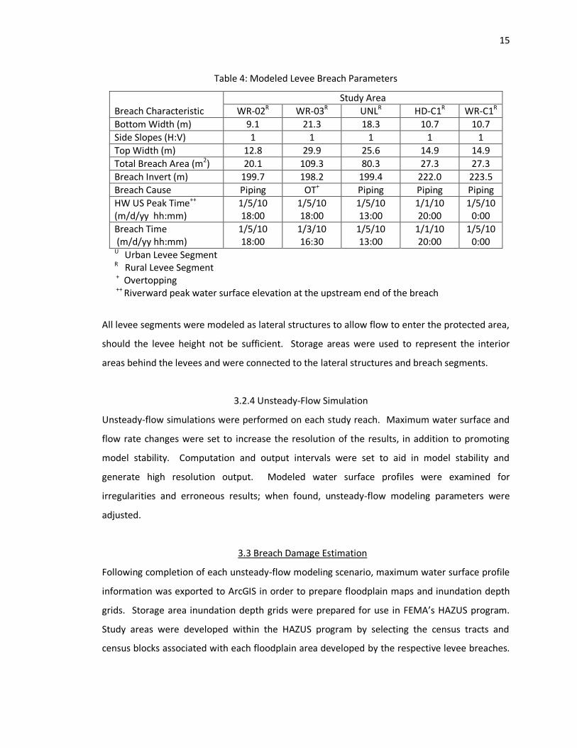
river stage reached a peak value. Table 4 contains a summary of the modeled levee breaches.

15

Table 4: Modeled Levee Breach Parameters

Breach Characteristic

Study Area

WR-02R WR-03R UNLR HD-C1R WR-C1R

Bottom Width (m) 9.1 21.3 18.3 10.7 10.7

Side Slopes (H:V) 1 1 1 1 1

Top Width (m) 12.8 29.9 25.6 14.9 14.9

Total Breach Area (m2) 20.1 109.3 80.3 27.3 27.3

Breach Invert (m) 199.7 198.2 199.4 222.0 223.5

Breach Cause Piping OT+ Piping Piping Piping

HW US Peak Time++

(m/d/yy hh:mm) 1/5/10 18:00

1/5/10 18:00

1/5/10 13:00

1/1/10 20:00

1/5/10 0:00

Breach Time (m/d/yy hh:mm)

1/5/10 18:00

1/3/10 16:30

1/5/10 13:00

1/1/10 20:00

1/5/10 0:00

U Urban Levee Segment R Rural Levee Segment + Overtopping ++ Riverward peak water surface elevation at the upstream end of the breach

All levee segments were modeled as lateral structures to allow flow to enter the protected area,

should the levee height not be sufficient. Storage areas were used to represent the interior

areas behind the levees and were connected to the lateral structures and breach segments.

3.2.4 Unsteady-Flow Simulation

Unsteady-flow simulations were performed on each study reach. Maximum water surface and

flow rate changes were set to increase the resolution of the results, in addition to promoting

model stability. Computation and output intervals were set to aid in model stability and

generate high resolution output. Modeled water surface profiles were examined for

irregularities and erroneous results; when found, unsteady-flow modeling parameters were

adjusted.

3.3 Breach Damage Estimation

Following completion of each unsteady-flow modeling scenario, maximum water surface profile

information was exported to ArcGIS in order to prepare floodplain maps and inundation depth

grids. Storage area inundation depth grids were prepared for use in FEMA’s HAZUS program.

Study areas were developed within the HAZUS program by selecting the census tracts and

census blocks associated with each floodplain area developed by the respective levee breaches.

16

Default building stocks and infrastructure data were used for each study area to maintain the

comparability of the levee segments. Local, spatially-referenced infrastructure information was

not available for all of the study areas; therefore, no user-defined infrastructure components

were added to any of the study areas due to a lack of comprehensive data.

Analyses were carried out to assess the amount of damage and economic loss expected for each

of the protected areas. Loss estimates were developed for building, agricultural, transportation,

utility, and vehicle losses. Income and inventory losses were included in the building loss

estimate for each study area.

3.4 Improvement Cost Assessment

The high resolution DEM data, aerial photography, and site inspections were used to aid in the

development of expected levee improvement costs. Deficiencies were identified by using the

required qualities of a certified levee based on 44 CFR 65.10. The requirements of this federal

regulation are summarized in Table 5 (FEMA, 2008).

Table 5: Requirements of 44 CFR 65.10

The Flood Insurance Study flood profile for the WFK White River and Howland Ditch were used

to develop the minimum required levee crest elevations for each segment. Cross-sections of the

existing levee were generated from the LiDAR DEM. Typical levee cross-sections were projected

onto the existing cross-sections to determine the quantity of cut and fill, as well as the extent of

surface disturbance and surface restoration. The typical levee cross-section used in the analyses

44 CFR 65.10

Criteria Design Requirements

Freeboard Levee must be constructed with a minimum of 3 - 4.5 ft of freeboard above the effective base flood profile (1%-annual-chance flood water surface profile)

Penetrations

Provide positive backflow prevention in the form of sluice gates and/or flap gates/check

valves/bolt-down lids on all storm and sanitary sewers penetrating through or under the

levee to prevent flooding of interior areas.

Stability Provide a stable foundation for all levees/floodwalls. Remove all material which may

compromise long term stability. Install foundation drains to prevent piping failure.

Settlement Construct levee to a height such that any anticipated settlement over time will not result

in freeboard below the minimum requirements.

Interior

Drainage

Provide for interior drainage by using gravity sewers and/or pump stations such that

interior ponding areas do not develop during coincident rainfall and flooding events.

17

is shown in Figure 5. The USACE requires that no woody vegetation be present within fifteen

feet of the levee toe (USACE, 2000). The extent of tree removal was determined by a

combination of aerial photography and the levee cross-sections generated from the LiDAR DEM.

Figure 5: Typical Levee Cross-section

Other critical aspects of determining the repair cost of a levee include the number of storm and

sanitary sewer penetrations, the condition of the underlying soil material, the existence and

condition of interior drainage systems, and the number and size of necessary openings in the

line of protection. Detailed topographic and utility surveys are necessary to develop the

number of underground utilities passing under, or through, the levee; this work is often time

consuming and expensive for large areas. As a result, underground utilities were not considered

in the improvement estimates for the study area levee segments. The number and condition of

visible backflow prevention devices needed for culverts and pipes was determined during site

inspections. The physical properties of the levee’s parent materials can only be determined by a

physical investigation including soil borings in the vicinity of the levee. The geotechnical

investigation required to assess the condition of base soil materials is similarly expensive and

time consuming; therefore, this consideration was not included in this study. Current local unit

cost estimates were used (CBBEL, 2011) to convert the necessary improvements to dollars of

expected construction cost. Engineering judgment and industry standards were used to

determine the approximate site survey, geotechnical, and design fees for each levee segment.

18

CHAPTER 4 STUDY AREA RESULTS

4.1 Hydraulic Results for Levee Breaches

Due to differences in protected area size, topography, flooding source, as well as levee

characteristics, the resulting breach floods were wide-ranging. Flooding duration was

accounted for by the length of time during which water was flowing into, or out of the storage

area in appreciable amounts. By using this method of determining flooding duration, the

duration required to dewater the interior area below the bottom of the levee breach is not

considered. The data requirements necessary to adequately describe the dewatering time is

beyond the necessary scope for the intended purpose of this analysis. A summary of the breach

results is shown in Table 6.

Table 6: Levee Breach and Storage Area Results

Storage Area

Max Stage (m)

Max Inflow (m3/s)

Peak Storage (Mm3)

Flood Area (km2)

Flooding Duration (days)

WR-C1U 224.12 24.9 1.2 0.8 6.0

HD-C1U 222.78 20.1 0.4 0.4 5.0

UNLR 201.03 159.9 8.7 6.4 8.8

WR-02R 201.15 25.4 0.2 0.1 4.1

WR-03R 202.76 150.9 0.3 0.1 6.1 U Urban Levee Segment R Rural Levee Segment

4.1.1 Storage Area Stage and Flow Hydrograph Analysis

Unsteady-flow modeling using storage areas provides the opportunity to assess the details of

the system response to the levee breach. The resulting stage and flow hydrographs can be

examined to extract critical information regarding the nature of the flooding behind the levee as

well as the key factors which caused the flooding to occur in the manner predicted by the

model.

19

The results of an unsteady-flow analysis of a levee breach in WR-C1, shown in Figure 6, reveals a

relatively moderate peak breach inflow. The stage hydrographs proximate to the levee breach

suggest that the peak water surface elevation achieved in the storage area is significantly less

than the stage in the main river channel. A reduction in water surface elevation is created by

the lag between the peak of the river hydrograph and the peak in the storage area hydrograph.

The unsteady-flow modeling allows for an approximation of the time required for the interior

and exterior stages to equalize. Based on the model results, the flood stage behind the

breached levee will not decrease as fast as the exterior river stage which is due to the small

breach size relative to the size of the WR-C1 storage area. The duration of the flooding behind

the levee is expected to be lengthened by this phenomenon.

Figure 6: WR-C1 Stage and Flow Hydrographs

20

Though HD-C1 and WR-C1 protect the same area, a breach in HD-C1 is expected to produce a

significantly different flood as compared to a breach in WR-C1. The impact of the difference in

flooding source can be seen by noting several key changes in the shape of the stage and flow

hydrographs in Figure 7. The first is the timing of the flooding. The peak of the Howland Ditch

stage hydrograph, shown in series ‘Stage HW US’ in Figure 7, occurs much earlier than that of

the WFK White River peak. The second and most notable difference is the difference in the

magnitude and duration of flooding. The flooding resulting from a breach in HD-C1 is expected

to create a flood stage that is 1.34 meters lower than the flooding caused by a breach in WR-C1,

with a flood duration one day less.

Figure 7: HD-C1 Stage and Flow Hydrographs

21

The connectivity of Howland Ditch to WFK White River also causes a slight amount of inflow to

the storage area significantly after the levee breach has allowed the interior and exterior flood

stages to equalize. If the flooding along WFK White River were more severe, a second rise in

flood elevations behind the levee would have occurred due to increased backwater. Though the

second flood wave experienced behind the failed levee was not severe, the prevention of flood

subsidence lengthened the duration of flooding by several hours. Had the second flood wave

been more severe, the duration could have been lengthened considerably.

22

The simulated levee breach in UNL suggests a more intense and severe flood wave into the area

behind the levee. The height of the levee and the flooding capacity of the WFK White River are

apparent in the magnitude of the peak inflow to the storage area. The breach diverts a

sufficient amount of flow from the WFK White River to noticeably decrease the stage of the

river during the initial levee breach. Inflow to the area behind the levee began to occur before

the levee breach as a result of downstream portions of the levee having insufficient height. The

flooding created by the levee overtopping alone has a relatively minor impact compared to the

breach at the upstream end of the levee. Despite the large breach inflow, the storage capacity

of the interior area and the insufficient downstream levee elevations prevent the equalization

with the exterior flood stage for approximately 52 hours. Figure 8 contains the stage and flow

hydrographs for the UNL levee breach model simulation.

Figure 8: UNL Stage and Flow Hydrographs

23

Figure 9 displays the reaction of the storage area behind WR-02 to a levee breach at the

upstream end of the levee segment. The size of the storage area behind WR-02 plays a

significant role in the system’s response to the levee breach. Despite the small breach area, the

flood stage on the interior of the levee equalizes with the exterior stage within a matter of

hours. The storage area filled to the level of the exterior flooding before the exterior flooding

could begin to subside, allowing no reduction in flood elevation. The absence of a lag time

between interior and exterior peak flood stage equalization suggests that the storage area could

be modeled accurately using a steady-state model simulation; however, it is apparent from the

other analyses that this is not a universal trait of levee breaches. The quick response time of the

storage area behind WR-02 allows the storage area stage to lower at the same rate as the main

river, preventing any extension of flood duration.

Figure 9: WR-02 Stage and Flow Hydrographs

24

The levee breach simulation for WR-03 was initiated by overtopping prior to the peak flood

elevation along WFK White River. As a result, the area behind the levee is filled to the level of

the WFK White River before the flood crests. The storage capacity behind WR-03 is quite small

in comparison to the levee breach flow capacity, resulting in a near instantaneous filling of the

area behind the levee. Insufficient levee height along the majority of the levee’s length allows

for constant interaction with WFK White River. This interaction results in a slight amount of

instability within the model, as can be seen in the ‘Net Inflow’ series of the Storage Area plot in

Figure 10. By inspecting the stage hydrographs associated with the levee breach, one can

determine that the amount of flow both into and out of the storage area during this period of

high fluctuation result in minor increases and decreases in stage, which suggests a negligible

inflow value.

Figure 10: WR-03 Stage and Flow Hydrographs

25

The storage areas behind WR-C1, HD-C1, and UNL exhibit a considerable reduction in water

surface elevation created by the lag between the peak of the river hydrograph and the peak in

the storage area hydrograph. Longer equalization time, or time required for the interior and

exterior stages to reach equilibrium, corresponds to a greater reduction in flood stage. A

summary of the equalization time and stage loss for each storage area is shown in Table 7.

Table 7: Breach Equalization Time and Stage Loss Results

Breach Characteristic

Study Area

WR-02R WR-03R UNLR HD-C1R WR-C1R

Breach Time (m/d/yy hh:mm)

1/5/10 18:00

1/3/10 16:30

1/5/10 13:00

1/1/10 20:00

1/5/10 0:00

EQ Time (m/d/yy hh:mm)

1/5/10 21:00

1/3/10 17:00

1/7/10 16:00

1/2/10 12:00

1/5/10 20:00

Equilization Time (hrs) 3.0 0.5 51.0 16.0 20.0

Stage Loss (m) 0.0 -0.1 1.4 1.3 1.0 + Overtopping ++ Riverward peak water surface elevation at the upstream end of the breach

4.1.2 Inundation Areas and Depth Grids

Inundation area maps and depth grids were created to determine the geographic extent of the

flooding, locations of extreme flooding, and to assess the validity of the assumption of perfect

hydraulic connectivity within the storage areas behind the levee segments. Storage volumes

and storage areas were compared to the total storage volume and area of the respective levee

segments to determine the level of storage and floodplain consumption.

26

The floodplain resulting from a breach in WR-C1 is expected to produce a floodplain that

consumes 80-percent of the surface area of the storage area and 87-percent of the storage

volume. The most extreme flooding within the storage area occurs in the multi-family

residential area in the northern portion of the flooded area, as depicted in Figure 11. The depth

of flooding within the storage area is relatively consistent with an average of 1.5 meters of

depth. The continuous nature of the flooded are suggests that the assumption of perfect

hydraulic connectivity is reasonable for the given application and breach scenario.

Figure 11: WR-C1 Levee Breach Depth Grid

27

The less severe flooding of the urban study area caused by a breach in HD-C1 produces a

floodplain area that inundates approximately 42-percent of the total surface area and utilizes

46-percent of the storage volume. The low-lying residential area is once again the site of the

most extreme flooding. Flood depths, shown in Figure 12, have an average of 0.9 meters.

Though the floodplain area is not fully connected, it is plausible that overland flow could have

allowed for substantial temporary hydraulic connectivity of the two main flooding areas.

Figure 12: HD-C1 Levee Breach Depth Grid

28

Flooding within the storage area behind UNL occurs mainly in the southern portion of the

protected area, as the land slopes generally to the south. Agricultural lands in the south are

affected most heavily by the resulting flood. The levee breach is expected to allow for 88-

percent of the available floodplain area to be covered by water, and 49-percent of the storage

volume to be filled by the flood. Flood waters are expected to average 1.8 meters in depth. The

depth grid shown in Figure 13 reveals a flood boundary with significant disconnects; therefore

the assumption of perfect hydraulic connectivity appears to be slightly less plausible for the UNL

storage area.

Figure 13: UNL Levee Breach Depth Grid

29

The size and relatively uniform topography of WR-02 creates a similarly uniform flood depth

throughout the storage area. The average flood depth is 1.9 meters. The floodplain

encompasses 98-percent of the total area, and 99-percent of the storage volume is consumed.

The small size of the protected region and fact that the flood boundary nearly covers the entire

area agree with the assumption of perfect hydraulic connectivity. The depth grid for WR-02 is

shown in Figure 14.

Figure 14: WR-02 Levee Breach Depth Grid

30

The flooded area behind WR-03 is quite similar to WR-02. The storage area is small and has

consistent flood depths over the whole surface; the flood depths have an average value of 1.8

meters. The flood is expected to cover 100-percent of the total area, and occupy 100-percent of

the total storage volume available. As with WR-02, the size and connectivity of the flooded area

suggest that the assumption of perfect hydraulic conductivity is valid. Figure 15 shows the

depth grid for the flood resulting from a levee breach in WR-03.

Figure 15: WR-03 Levee Breach Depth Grid

31

4.2 Breach Damage Estimation Data

Expected losses for the levee breaches ranged significantly as a result of the varying levee

lengths, levee heights, size of protected area, as well as with the type and number of buildings

protected. Table 8 contains a summary of the losses due to the flooding caused by the levee

breaches. Appendix D contains more detailed information concerning the losses determined by

HAZUS.

Table 8: Breach Damage Summary

Storage Area

Breach Damage Parameters

Building Losses

(x $1000)

Agricultural Losses

(x $1000)

Transportation Losses

(x $1000)

Utility Losses

(x $1000)

Vehicle Losses

(x $1000)

Displaced Citizens

(#)

TOTAL BREACH

DAMAGES (x $1000)

WR-C1U $24,794 $0 $0 $0 $2,395 391 $27,189

HD-C1U $5,950 $0 $0 $0 $757 212 $6,707

UNLR $12,231 $157 $0 $0 $1,158 174 $13,545

WR-03R $64 $3 $0 $0 $5 1 $72

WR-02R $82 $2 $0 $0 $7 1 $91 U Urban Levee Segment R Rural Levee Segment

No spatial data was available for local roads, railways, and bridges within the study areas; only

state-owned infrastructure components were considered in the loss analysis. Utilities

considered in the analysis were limited to key components of utility systems such as electrical

substations, water and wastewater pump stations; these components were not impacted by the

flood areas developed by the levee breaches.

4.3 Improvement Cost Data

Each levee segment had varying degrees of deficiency, with some needing only minor

improvements and others requiring virtual reconstruction. Expected improvement costs ranged

as widely as the levees’ impaired condition. The large disparity in levee size creates an equally

large gap in the amount of funding necessary to improve the levees. The most influential levee

deficiencies were tree cover, inadequate levee height, and over-steepened side slopes. In the

case of the rural levees, these deficiencies necessitate the disturbance of large areas of land

leading to increase demolition and reclamation costs. Design and permitting fees of extensive

32

repairs were also included as a percentage of the construction cost, which further increased the

difference between the rural and urban levee segments as the urban levee segments will

require less extensive permitting due to the decreased disturbance areas.

Table 9 contains a summary of the expected improvement costs for each of the levee segments.

A more detailed form of the improvement cost estimates can be seen in Appendix E.

Table 9: Improvement Cost Summary

Storage Area

Improvement Cost Parameters

Demolition (x $1000)

Levees & Bank

Stabilization (x $1000)

Site Restoration

(x $1000) Drainage (x $1000)

Misc. (x $1000)

Professional Services

(x $1000) Total Cost (x $1000)

WR-C1U $0 $67 $215 $47 $216 $74 $650 HD-C1U $0 $8 $79 $47 $83 $30 $252

UNLR $482 $2,050 $1,930 $47 $3,390 $899 $9,938 WR-03R $101 $473 $397 $12 $744 $218 $2,201

WR-02R $84 $429 $341 $0 $649 $190 $1,920 U Urban Levee Segment R Rural Levee Segment

33

CHAPTER 5 CONCLUSIONS

The condition of existing levees and lack of sufficient funding in the United States demonstrates

a need for a standardized method of assessing the risk for home, land, and business owners

whose property is situated behind a levee. The modeling and analysis procedures set forth in

this study are capable of limiting the risk to both the properties in jeopardy and the limited

funds available by prioritizing levees in order for decision makers to attain the highest possible

return-on-investment. The results of the analysis have identified key components of levee

breach assessment for prioritizing levee rehabilitation, including:

5.1 Unsteady-flow Modeling

The use of unsteady-flow modeling provides more information concerning the hydraulic

system’s response to a levee breach as well as producing more realistic results. Regulatory

models utilize a steady-flow analysis which produces more conservative flood elevations;

however, the procedure used in this study is not suggested for use in regulatory floodplain or

floodway determination. Based on the intended use, the more realistic nature and increased

amount of information provided by an unsteady-flow analysis is warranted. The purpose of

prioritizing levees is to appropriate funds in the most beneficial way. For this to occur, a

realistic, yet somewhat conservative view must be employed. Unsteady-flow modeling allows

for the use of storage areas within HEC-RAS to determine the potential flood depths behind a

levee rather than modeling the area as a flowpath for the channel. Simply ignoring that a levee

exists is to ignore the true physical nature of the system. A levee breach may be quite small

relative to the size of the protected area, preventing the consumption of all storage volume

behind the levee prior to subsidence of riverine flooding. Storage areas behind levees may not

fill to the peak water surface elevation along the river, or to the top of the levee crest during a

flooding event, which are the possible floodplain determinations by current standards of

practice. This is made evident by the results expounded upon in Section 4.1.1.

34

An examination of steady-state analyses of the same study segments reveals a large disparity

between the predicted flood elevations. The steady-state flood elevations shown in Table 10

were produced using the peak flow rate from the unsteady-flow hydrographs for each study

area channel reach. A comparison of unsteady-flow and steady-state flood depth grids can be

seen in Appendix A.

Table 10: Comparison of Unsteady and Steady-flow Flood Elevations

Storage Area

Unsteady-flow

Max Stage (m)

Steady-flow Max Stage

(m)

Unsteady-flow

Peak Storage (Mm

3)

Steady-flow Peak

Storage (Mm

3)

Unsteady-flow

Flood Area (km

2)

Steady-flow Flood Area

(km2)

WR-C1U 224.12 224.96 1.2 1.7 0.8 1.0

HD-C1U 222.78 223.70 0.4 0.9 0.4 0.7

UNLR 201.03 Varies 8.7 13.2 6.4 6.6

WR-02R 201.15 201.14 0.2 0.2 0.1 0.1

WR-03R 202.76 202.82 0.3 0.3 0.1 0.1 U Urban Levee Segment

R Rural Levee Segment

Finally, unsteady-flow analyses consider in-channel and floodplain storage of runoff. The runoff

flow hydrograph for Howland Ditch has a peak value of 55.4 m3/s; however, the peak flow

passing through much of the channels length in the model was 41.1 m3/s due to significant

storage of flow behind bridges and other obstructions.

5.2 Storage Areas

As mentioned in the discussion of steady versus unsteady-flow simulation, the use of storage

areas to represent the levee-protected areas more closely resembles the physical reality of the

situation than the current standard of practice. Steady-state models are incapable of

determining the duration of flooding, and are therefore not able to determine the impact of the

relative size of the levee breach and storage area on the duration of flooding. Larger storage

areas could experience increased flooding duration as a result of insufficient drainage of flood

waters. The physical extent of the breach and inadequacy of the drainage system supporting

the area may cause the area to retain the flood water at a higher stage than that experienced on

the riverward side of the levee.

35

5.3 Priority Ratio

Cost-benefit analyses are regularly performed to determine if it is economically practical to

construct a new levee. After a levee is constructed and is allowed to age and continue into a

state of disrepair, a new issue arises. Development behind the levee prevents the issue from

being solely economically based. Rather than questioning whether or not to build a levee,

decision makers must decide if and when to improve the levee. By using only the expected

damages resulting from a breach to prioritize levees, a tendency toward repairing larger levee

segments or levee segments in more affluent regions will become apparent. In order to more

wisely allocate funding, the cost of the repairs must also be considered. When comparing

levees WR-C1 and UNL using the expected damages alone, UNL has a higher ranking; when using

a ratio of expected damages to improvement cost, the priority ratio, WR-C1 has a higher

ranking. By using the priority ratio, investors should achieve a higher return-on-investment.

In addition to helping prioritize levees, the development of a larger dataset of analyses could

allow for determination of threshold ratio values to help suggest when decision makers should

improve or abandon levees or when to buyout the homes and properties behind the levees to

eliminate the hazard. The Property Acquisition Program currently run by FEMA focuses on

purchasing private properties in repetitive loss areas. The local or state government is required

to produce 25-percent of the total capital investment, while the remaining 75-percent is

covered by FEMA. To be considered for a buyout, the entire buyout area must be a part of the

National Flood Insurance Program; areas that have not elected to be included in the program

are not eligible for property buyout projects. Following a buyout, the land becomes public

property and must remain as open space, property resale and development is not an option.

The land may remain as open space or be converted to parks, wildlife refuges, or other

undeveloped, natural uses. (FEMA, 2010) The program has obvious benefits, both in terms of

risk reduction and environmental well-being; however, the reactive approach of the method

prevents continued risk, rather than eliminating risk before lives and property are lost. Utilizing

a threshold priority ratio to identify areas that are subject to unsatisfactory risk could achieve

the two-fold benefits of a buyout, without unnecessary exposure to flood damage and potential

loss of human life.

36

A lack of decisive correlation between hydraulic, zoning, social, breach damage, and

improvement cost statistics fails to provide a rule-of-thumb for determining levee priority. The

priority ratio can serve as a means of sequencing levee improvements and property buyouts, in

the absence of a simpler prioritizing scheme.

5.4 Decision Guidance and Project Justification

By using a standardized procedure and ranking levees against one another, decision makers may

experience less public opposition to flood control projects. Complete removal of all public

criticism is not likely, as risk assessments only constitute a small portion of regulatory control

(National Research Council, 1983). Risk management policy, or the regulatory actions taken as a

result of the risk analyses, may still be viewed with opposition. The presence of quantitative

evidence of need for improvements and the sequence in which the improvements should be

made can be used to increase stakeholder buy-in. Efforts should be made to limit the

bureaucratic and political involvement in decision making and development of risk management

policy.

37

CHAPTER 6 TOPICS FOR FUTURE DEVELOPMENT

6.1 Loss-of-life Modeling

The value of human life cannot be overlooked in any risk assessment that attempts to be widely

applicable and accepted. Publicly available loss-of-life models have yet to be developed for

analyses such as the one described by this study. Highly complex loss-of-life models have been

used in other studies. The IPET study of the aftermath of Hurricane Katrina utilized proprietary

modeling software developed specifically for the analysis of the New Orleans disaster.

Development, or public release, of spatially referenced loss-of-life modeling software would

enable analysts to more appropriately factor in the impact of levee breach progression and the

rate at which floodwaters rise. Use of spatial reference would allow for the use of census data

to incorporate the age of endangered citizens, as well as the size of families within the impacted

areas.

6.2 Social and Cultural Impacts of Flooding

Social and cultural impacts of flooding disasters have been studied diligently in the recent years,

specifically during the IPET evaluation of Hurricane Katrina. Though the social and cultural

impacts were assessed, all data presented was strictly qualitative or anecdotal. A risk

assessment methodology that includes social and cultural impacts and is able to withstand

public criticism would require quantitative results. These results would likely need to be

translated into dollar figures by loss estimation or increases in impoverishment in order to be

combined with breach damage and improvement cost estimations. Valuing cultural and social

artifacts in monetary figures will likely be a challenging and highly subjective endeavor. Use of

‘willingness-to-pay’ surveys may allow for analysts to quantify an approximate value for the

endangered social and cultural stock.

38

6.3 Environmental Benefits of a Natural Floodplain

Quantification of environmental benefits of a natural floodplain suffers the same lack of

development as social and cultural aspects. Qualitative and anecdotal evidence of

environmental benefits is widely available. Unfortunately, disagreement exists between experts

in the environmental fields associated with riparian areas. Without a clear consensus of what

defines healthy, beneficial floodplain activity, inclusion of environmental benefits in an

economical valuation within a risk assessment will likely be met with much skepticism and

opposition.

6.4 Engineered Levee Breaches

Flooding along large rivers often develops over a substantial amount of time, which can allow

for human intervention to prevent catastrophic failures of flood control components. During

recent flooding along the Mississippi River, the USACE made an informed decision to remove

large portions of levee upstream of Cairo, Illinois. The added floodplain storage lowered the

peak flood elevation along the main river body by several feet, preventing potentially dangerous

stress on the aged levee system. Though the methodology set forth by this study is not

specifically intended for the use of assessing the value of storage areas for flood relief, it could

be easily adapted to do so. An evaluation of the damages expected if the levee were breached

versus the damages expected downstream would allow officials to make informed decisions,

knowing the approximate cost of either decision.

Another potentially useful modification of the proposed methodology would be to identify

deteriorated levees whose protected areas could serve as compensatory storage areas to

provide relief for overdeveloped floodplain areas. Buyout costs could be determined and

weighed against the expected reduction of economical risk. The evaluation could also be

expanded to include other components of the total risk if more adequate methods of

quantifying risk are developed.

39

6.5 Levee Breach Progression

Levee breach progression studies show that the development of earthen levee breaches is

highly variable and contingent upon data that is not easily nor economically acquired. As a

result, breach progression models having a high correlation to real-world breach scenarios are

lacking. The levee breach progression used by this methodology is over-simplified and confined

to a limited set of initiation processes. Breach flow rates are heavily dependent on the

assumptions made concerning the size and progression of the levee breach. The height of the

levee essentially dictates the magnitude of the peak breach flow rate, when using the IDNR

guidelines for breach progression. As breach progression models increase in quality and

number, the type of breaches examined in the risk assessment could be expanded to include

multiple types of failure initiation and a wider application to levees with different physical

components. The breach progression models used in this study are based on grand assumptions

of uniform response to stress; however, the assumptions made are the current standard of

practice. The importance of breach progression is apparent in the results from this study.

Breach progression modeling will also serve as an important factor for any development in loss-

of-life modeling due to the impact on the rate at which floodwaters rise and the time available

for evacuation.

40

WORKS CITED

American Society of Civil Engineers. (2009). Report Card for American Infrastructure: Levees.

Baecher, G. B. (2009, September 8). Quantifying Flood Risk.

Bodenhamer, D. J., & Barrows, R. G. (Eds.). (1994). The Encyclopedia of Indianapolis. Indiana

University Press.

Chow, V. T. (1959). Open-Channel Hydraulics. Caldwell, NJ: The Blackburn Press.

Christopher B. Burke Engineering, Ltd. (2007, October 9). City of Indianapolis Levee Assessment

Summary. Indianapolis, Indiana.

Christopher B. Burke Engineering, Ltd. (2011). Southport AWT Levee Extension and

Improvements Opinion of Probable Costs.

Federal Emergency Management Agency. (2008). Fact Sheet: Requirements for Mapping Levees.

Federal Emergency Management Agency. (2005). Guidelines and Specifications for Flood Hazard

Mapping Partners.

Federal Emergency Management Agency. (2011, February). Indiana Flood Fact Sheet.

Federal Emergency Management Agency. (2010, August 11). Property Acquisition Projects

(Buyouts). Retrieved June 12, 2011, from Federal Emergency Management Agency:

http://www.fema.gov/government/grant/mitmeasures/buyoutshow.shtm

Federal Emergency Managment Agency. (2005). Flood Insurance Study for Marion County,

Indiana, All Jurisdictions.

Indiana Department of Natural Resources. (2001). General Guidelines for New Dams and

Improvements to Existing Dams in Indiana. Indianapolis.

Interagency Performance Evaluation Task Force. (2009). Performance Evaluation of the New

Orleans and Southeast Louisiana Hurrican Protection System. USACE.

Marion County, Indiana. (2010). GIS Data and Aerial Photography. Indianapolis, Indiana.

McCuen, R. H. (1998). Hydrologic Analysis and Design. Upper Saddle River, NJ: Prentice Hall.

National Committee on Levee Safety. (2009). Recommendations for a National Levee Safety

Program.

National Oceanic and Atmospheric Administration. (n.d.). Precipitation-Frequency Atlas of the

United States. 2 , 3.0.

41

National Research Council. (1983). Risk Assessment in the Federal Government: Managing the

Process. Washington D.C.: National Academies Press.

National Research Council. (2009). Science and Decisions: Advancing Risk Assessment.

Washington D.C.: National Academies Press.

National Research Council. (2004). Valuing Ecosystem Services. The National Academy of

Sciences.

Natural Resource Conservation Service. (2010). SSURGO .

Norquest, C. E. (1913). March 1913 Flood. Retrieved June 25, 2011, from

http://www.crh.noaa.gov/ind/?n=march_1913_flood

Scawthorn, C. (2006). HAZUS-MH Flood Loss Estimation Methodology. II. Damage and Loss

Assessment. Natural Hazards Review , 72-81.

United States Army Corps of Engineers. (2000). Design and Construction of Levees.

United States Army Corps of Engineers. (2006). National Levee Database. Retrieved January 14,

2011, from http://www.usace.army.mil

United States Geological Survey. (2010). National Elevation Dataset. Retrieved January 11, 2011,

from http://seamless.usgs.gov/

United States Geological Survey. (2006). National Land Cover Database.

United States of America. (2009). Code of Federal Regulations .

APPENDICES

42

Appendix A – Flood of Record: 1913

The more recent flooding in Indiana, though significant, pales in comparison to the disastrous

effect of an unusually large rainfall event in the spring of 1913. C. E. Norquest, a local

newspaperman, provided a detailed description of the flooding and associated damages shortly

after the flood. Norquest explained that in late March, a string of several days of rainfall led to a

tremendous amount of runoff. Though the depth of rainfall was not unprecedented, the

uniformity of rainfall over the entire watershed had a devastating effect. An average of 7.81

inches of rain fell over a 48 hour period, resulting in the highest flood elevations recorded for

the WFK White River. The high rate of rainfall and saturated soils led to rapid river response to

the rainfall. The river stage increased a total of 14 feet in a span of three days, surpassing the

previous flood of record by 6 feet (Norquest, 1913).

Though Indianapolis had flood control infrastructure at the time, it was not capable of

containing the flood waters. A total of 6 square miles was inundated by WFK White River.

Several lowland areas in the city were entirely submerged by the raging river, and other areas

suffered partial or complete inundation due to levee failures. Advance warning of failing levees

allowed for a nearly complete evacuation of the affected areas, decreasing the loss-of-life

considerably. Flooding over such a large area of a highly populated region undoubtedly causes a

considerable amount of damage. A total of 12 fatalities resulted from the Flood of 1913, 5 of

which occurred in Indianapolis (Norquest, 1913). Floodwaters often force families from their

homes, leaving them displaced and without any recoverable personal items. The Flood of 1913

displaced approximately 4000 families as their homes were swallowed by the river. In addition

to private losses corporate damages were also realized during the flood event. A total of four

bridges were washed out as the flooded river neared its crest. Two of the bridges were the

property of railroad companies, one municipal bridge, and one private bridge. Though not

subject to floodwaters, the remainder of the city felt the impact of the flood as the local power

company’s boilers were put out by the elevated river, leaving the city without power. Without

power, the entire city was left more vulnerable to fire due to lack of electricity for water pumps.

Urban areas of the city were not the only areas suffering from the deluge of water, agricultural

areas experienced immediate losses, as well as prolonged effects from the flooding of farm

fields and pastures. Crops were destroyed and fields were left in poor conditions, with many

43

being left fallow in subsequent years due to the thick layers of sand deposits left by the receding

water. Rising water carried away some livestock and left many more stranded and lost

(Norquest, 1913).

The financial representation of the losses helps to establish a sense of the true scope of the

damage levied on Indianapolis. Property damage to homes, commercial and industrial

equipment, and bridges represent nearly half of the financial toll; the estimated property losses

totaled over $4.6 million. Agricultural losses in the amount of approximately $310,000 included

lost crops and livestock; expected losses due to the sand deposits creating infertile fields were

not included in the estimate. Economic losses were established by estimates of lost wages due

to forced suspension of labor and product sales reductions; the total estimated amount of

economic loss was $622,000 (Norquest, 1913). A significant amount of the total resulting losses

from the flood were associated with the bridges destroyed by the raging flood. A total of

approximately $4.8 million was recorded for damages to railroads and trolleys. The sum of all of

the losses measured in financial terms was $10.4 million for the city of Indianapolis; this equates

to nearly $230 million in 2010.

44

Appendix B- Hydrologic Modeling Data & Results

Figure B.1: Observed Peak Annual Streamflow vs. Log-Pearson Type III Distribution

Figure B.2: Stream Length vs. Contributing Watershed Area

45

Table B.1: Hydrologic Parameter Summary

Flooding Source

Hydrologic Parameter

Watershed Area (km2)

Average CN (-)

Tc (hrs)

Peak Flow

(m3/s)

Runoff Volume (Mm3)

Hydrograph Duration (days)++++

WFK White River+ 3026.6 80.5 90.3 954.4 261.9 10.5

WFK White River++ 4885.4 80.2 112.8 1037.1 392.5 13.9

Howland Ditch+++ 27.5 70.3 19.8 55.4 2.3 2.3 +

At 82nd

Street bridge +++

At Dean Road

+ + At Southport Road bridge

++++ Duration of flow rates exceeding 0.1 m

3/s

Figure B.3: Watershed Areas and Ground Surface Elevation

46

Figure B.4: WFK White River Streamflow Hydrograph at 82nd Street Bridge

Figure B.5: Howland Ditch Streamflow Hydrograph at confluence with WFK White River

47

Figure B.6: WFK White River Streamflow Hydrograph at Southport Road Bridge

48

Appendix C– Hydraulic Modeling Results

Figure C.1: Unsteady-flow vs. Steady-state Floodplain Boundaries for HD-C1 Levee Breach

Figure C.2: Unsteady-flow vs. Steady-state Floodplain Boundaries for WR-C1 Levee Breach

49

Figure C.3: Unsteady-flow vs. Steady-state Floodplain Boundaries for WR-C1 Levee Breach

50

Appendix D – Breach Damage Estimation

Table D 1: Summary of HAZUS Breach Damage Estimation

Economic Loss Type

Breach Damage ($ in thousands )

WR-C1 HD-C1 UNL WR-02 WR-03

Building Losses

Structure $12,206 $2,538 $5,067 $37 $46

Contents $12,440 $3,368 $7,091 $27 $35

Income $148 $44 $73 $0 $1

Total Building Losses: $24,794 $5,950 $12,231 $64 $82

Agricultural Losses

Corn $0 $0 $154 $3 $2

Soybeans $0 $0 $0 $0 $0

Wheat $0 $0 $3 $0 $0

Total Agricultural Losses: $0 $0 $157 $3 $2

Transportation Losses

Highway $0 $0 $0 $0 $0

Railway $0 $0 $0 $0 $0

Total Transportation Losses: $0 $0 $0 $0 $0

Utility Losses

Potable Water $0 $0 $0 $0 $0

Waste Water $0 $0 $0 $0 $0

Oil Systems $0 $0 $0 $0 $0

Natural Gas $0 $0 $0 $0 $0

Electric Power $0 $0 $0 $0 $0

Communication $0 $0 $0 $0 $0

Total Utility Losses: $0 $0 $0 $0 $0

Vehicle Losses

Daytime Flood $2,395 $757 $1,158 $5 $7

Nighttime Flood $2,293 $649 $918 $5 $7

Total Vehicle Losses: $2,395 $757 $1,158 $5 $7

Displaced Citizens 391 212 174 1 1

TOTAL BREACH DAMAGES: $27,189 $6,707 $13,545 $72 $91

51

Appendix E – Improvement Cost Estimates

52

53

54

55

56

Appendix F – Levee Prioritization Statistics

Table F.1: Priority Ratio vs. Hydraulic Statistics

Storage Area

Damage: Cost Ratio

Levee Priority

Hydraulic Parameters

Max Stage (m)

Max Inflow (m3/s)

Peak Storage (Mm3)

Flood Area (km2)

Flooding Duration

(days)

HD-C1U 26.62 2 222.78 20.11 0.4 0.4 5.0

WR-C1U 41.84 1 224.12 24.88 1.2 0.8 6.0

UNLR 1.36 3 201.03 159.90 8.7 6.4 8.8

WR-03R 0.05 4 202.18 150.86 0.2 0.1 6.1 WR-02R 0.03 5 201.15 25.43 0.2 0.1 4.1 U Urban Levee Segment R Rural Levee Segment

Table F.2: Priority Ratio vs. Zoning Statistics

Storage Area

Damage: Cost Ratio

Zoning & Development Parameters

Residential (%)

Commercial (%)

Special Use (%)

Agricultural (%)

Park (%)

Buildings (#)

Density (Bldg / ac)

HD-C1U 26.62 76.6 11.3 12.1 0.0 0.0 880 1.64

WR-C1U 41.84 76.6 11.3 12.1 0.0 0.0 880 1.64

UNLR 1.36 46.0 3.0 7.1 43.9 0.0 1711 0.61

WR-03R 0.05 0.0 0.0 0.0 42.0 58.0 0 0.00

WR-02R 0.03 0.0 0.0 0.0 10.3 89.7 4 0.05 U Urban Levee Segment R Rural Levee Segment

57

Table F.3: Priority Ratio vs. Social Statistics

Storage Area

Damage : Cost Ratio

Social Parameters

Average Household Income

(x $1000)

Avg. Property Value

(x $1000)

Buyout Cost

(x $1M) Caucasian

(%)

Black / African American

(%) Asian (%)

Other Race (%)

HD-C1U 26.62 $60 $279 $279.0 68.2 27.0 1.4 3.4

WR-C1U 41.84 $60 $279 $279.0 68.2 27.0 1.4 3.4

UNLR 1.36 $53 $55 $94.2 94.8 1.7 1.1 2.4

WR-03R 0.05 $0 $0 $0.00 0.0 0.0 0.0 100.0

WR-02R 0.03 $0 $13 $0.04 0.0 0.0 0.0 100.0 U Urban Levee Segment R Rural Levee Segment

Table F.4: Priority Ratio vs. Breach Damage Statistics

Storage Area

Damage : Cost Ratio

Breach Damage Parameters

Building Losses

(x $1000)

Agricultural Losses

(x $1000)

Transportation Losses

(x $1000)

Utility Losses

(x $1000)

Vehicle Losses

(x $1000)

Displaced Citizens

(#)

TOTAL BREACH DAMAGES (x $1000)

HD-C1U 41.84 $5,950 $0 $0 $0 $757 212 $6,707

WR-C1U 26.62 $24,794 $0 $0 $0 $2,395 391 $27,189

UNLR 1.36 $12,231 $157 $0 $0 $1,158 174 $13,545

WR-03R 0.05 $64 $3 $0 $0 $5 1 $72

WR-02R 0.03 $82 $2 $0 $0 $7 1 $91 U Urban Levee Segment R Rural Levee Segment

58

Table F.5: Priority Ratio vs. Improvement Cost Statistics

Storage Area

Loss : Cost Ratio

Improvement Cost Parameters

Demolition (x $1000)

Levees & Bank Stabilization

(x $1000)

Site Restoration

(x $1000)

Drainage (x

$1000) Miscellaneous

(x $1000)

Professional Services

(x $1000)

Total Cost

(x $1000)

HD-C1U 41.84 $0 $8 $79 $47 $83 $30 $252

WR-C1U 26.62 $0 $67 $215 $47 $216 $74 $650

UNLR 1.36 $482 $2,050 $1,930 $47 $3,390 $899 $9,938

WR-03R 0.05 $101 $473 $397 $12 $744 $218 $2,201

WR-02R 0.03 $84 $429 $341 $0 $649 $190 $1,920 U Urban Levee Segment R Rural Levee Segment

59

Appendix G– Further Considerations

Lack of funding or excessive delays could prevent levees from being improved before a failure occurs.

As described previously, the timeliness of risk assessment results is often more important than the

absolute accuracy of the results. The methodology described provides a simplified process of analysis by

utilizing existing information and making reasonable and conservative assumptions, which allows for a

quick analysis turnaround. The relatively small time requirement to replicate the analysis could allow

for a more widespread assessment of levees, which, in turn, could lead to a better allocation of available

funding.

The method set forth in this study attempts to establish a relative scale used to compare and prioritize

levees based on the economic losses expected from a levee breach. The process involves the

development of hydrologic and hydraulic models, assessment of existing infrastructure, determination

of breach damages, and the estimation of improvement costs for the levee.

Key Components of Risk Assessment Strategies

The use of risk assessments to help prioritize levee rehabilitation requires the determination of key

factors in the design of the risk assessment strategy. Risk assessments must address three main

features of a given situation, in the case of this analysis, a flood. The first component of a risk

assessment is the determination of the hazard level, or the probability that the event will actually occur.

The vulnerability to the hazard is the likelihood that the event will have an unfavorable outcome. The

third component is the consequence, which is often described by the negative cost impact of a given

scenario (Baecher, 2009). Though the consequence is often identified by the negative outcome, it

should be noted that many events have both positive and negative results. Natural floodplains provide

a number of services; flood protection, pollution abatement, groundwater recharge, and increased

biodiversity are all potential benefits of maintaining an active and natural floodplain (National Research

Council, 2004). In addition to the three key components, risk assessments must consider the use of the

information developed.

Other factors, beyond the easily quantifiable components, can have an effect on the design of a risk

assessment. The intended use of the risk assessment can affect the desired output. For instance, if it is

known that a levee will suffer a catastrophic failure if a flooding event occurs, the absolute magnitude

60

and precision of the expected damages is less important than releasing the results of the study as

quickly as possible to allow for proper action. Another important aspect of risk assessment concerns the

audience to which the study is directed. Stakeholder involvement is essential for risk assessment design

to provide meaningful results (National Research Council, 2009) Budget committee members and

members of historical societies will likely view the expected flood damages from a levee breach quite

differently. One could anticipate that the budget committee members would be interested in how

much economic loss is expected compared to the cost to prevent the damages; one might also surmise

that the historical society members would be focused on what it would take to protect the artifacts

within the damaged area, with little regard for the cost of such protection. The risk assessment

methodology presented in this study is designed with these key components in mind. The applicability

of the methodology to any given levee system is also heavily considered when determining what output

will best address the risk associated with deteriorating levees.

The highly variable nature of the physical systems responding to the hazard creates a need to establish

default decision options within the risk assessment. For the purpose of comparability and prioritization,

the suggested default decision options have been selected to be impartial and conservative in nature.

Conservative assumptions are warranted when significant data gaps exist. Use of conservative

assumptions is reasonable in priority-setting assessments, such as the methodology described in this

study (National Research Council, 1983). The hazard level has been fixed for all analyses performed.

The 1%-annual-chance rainfall event has been selected to serve as the design event. The vulnerability of

the levee system has also been fixed; the methodology detailed herein assumes that all levees will

breach during the 1%-annual-chance flooding event. This leaves only the consequence to serve as the

differentiating component of the risk assessment. The intended use of this process is to help decision

makers maximize the return-on-investment of flood control infrastructure rehabilitation. As a result,

the data output developed is highly quantitative and economically based.

61

Current Standards of Practice

A large inventory of floodplain maps have been developed through FEMA’s various flood map

development programs, which are all a part of the National Flood Insurance Program. These programs

have been instituted to increase the public awareness of the hazard of flooding as well as to help reduce

the risk to human life and human investments. The results of flood mapping projects must be submitted

to FEMA for approval based on the guidelines developed by FEMA. Currently, flood maps are developed

using a steady-state flow regime to generate expected water surface profiles. Several steady-state flow

rates are used in the analyses; peak runoff from the 0.2%, 1%, 2%, and 4%-annual-chance events is

simulated (FEMA, 2005). The water surface profiles are then compared to existing topography to

determine the extents of the flooding along the river system for the various risk classes. Flood areas

being delineated within the 1%-annual-chance flood boundary are considered high risk areas, or Special

Flood Hazard Areas.

Flood mapping for areas protected by levee systems are assessed in a slightly different manner. If

levees are deemed capable of providing protection for the 1%-annual-chance event, and meet the

requirements of 44 CFR 65.10, the area behind the levee is shaded as and labeled ‘Zone X’ or ‘Zone AH’.

Shaded ‘Zone X’ denotes areas that have a moderate risk of flooding, or risk between 0.2% and 1%-

annual-chance of occurrence. ‘Zone AH’ identifies areas that are at risk of shallow flooding during the

1%-annual-chance event. In the event that a portion of a levee is not capable of meeting the

requirements of 44 CFR 65.10, the base flood elevation behind the levee is set equal to the water

surface elevations generated by modeling the system as if the levee did not exist (FEMA, 2005). The

floodplain boundaries delineated behind levees essentially provide the flooding if the levee were to

have never been built, or if the levee were to be removed entirely.

62

Risk assessments for areas prone to flooding currently utilize FEMA’s HAZUS program to develop the

expected economic risk posed by flooding. Currently regulatory models are used to determine the

extents of flooding. Depth grids or floodplain boundaries are used to within the HAZUS program to

produce the expected losses associated with the defined flooding. For areas that do not have hydrologic

and hydraulic models, floodplain extents can be determined in HAZUS using simplified hydrologic and

hydraulic methodologies.

In 2009, the Interagency Performance Evaluation Task Force completed an in depth risk assessment of

Hurricane Katrina. The post-hurricane assessment was used to predict the future risk to flooding based

on redevelopment scenarios. Experts from multiple engineering fields were employed to precisely

capture the reaction of the hydraulic system and the impacts of the flooding. Model calibration was

performed using extensive survey data collected after the flooding had subsided and recovery efforts

were underway. In addition to monetary loss estimates, the study attempted to identify the social,

cultural, and environmental impacts of the flooding. Loss-of-life modeling was performed for the

impacted areas and compared to the real-world data. (IPET, 2009) The volume and quality of data used

within the risk assessment, as well as the expertise of the individuals carrying out the assessment was

unprecedented.

Hydrologic Model Development

The development of hydrologic models is a complex and well-studied topic. Many federal and state

agencies, as well as some municipalities have their own particular guidelines for hydrologic model

development. Two options are considered for hydrologic model development, the use of existing

regulatory hydrologic models, and the development of entirely new hydrologic models. To maintain the

economic feasibility of performing hydrologic analysis on an extensive levee system, it is desirable to use

the most up to date and available data, rather than creating an entirely new hydrologic model. These

models are updated on a decennial basis or more frequently, and require significantly less modification

and data collection than areas without base flood models. In addition to reducing the amount of work

required to develop a model, the use of existing regulatory models ensures that the model has been

adequately reviewed and tested for unsound assumptions and errors. Larger streams and rivers

typically have hydrologic models available from Flood Insurance Studies required by FEMA. The obvious

benefits to using existing hydrologic models validate their use as the default option.

63

As an alternative to using existing hydrologic models, new models can be developed using the guidelines

set forth by the agency or government body having jurisdiction over the study area. This option is much

less desirable due to the amount of data collection and time necessary to review the models; however,

regulatory models do not exist for all streams, especially smaller tributaries which are heavily impacted

by the larger waterways to which they contribute. In cases where a new model must be developed, the

highest resolution data available can be utilized. High resolution soil, land use, and topography data are

publicly available for the United States from the USGS Seamless Server. Higher resolution data may be

available at the county or local level. USACE’s HEC-GeoHMS extension for geospatial software provides

an efficient and cost effective way to develop complex hydrologic models which are capable of using

high resolution data to describe the hydrologic response of a given watershed. The use of computer-

aided watershed delineation and curve number generation can help to eliminate subjective decision

making, helping to achieve the goal of unbiased assessments. Rainfall from the National Climate Data

Center on-line rain gage data and streamflow records from USGS stream gages can be used to calibrate

and verify the accuracy of the hydrologic model. However, by comparing two or more levees to each

other, the absolute accuracy of the data becomes less important compared to the relative accuracy

between the different analyses. To help maintain relative accuracy, the same approach, either

calibrated or un-calibrated, should be used for all levees being prioritized in a given study. The quality of

the data available to calibrate all models should be considered prior to determining whether a calibrated

or un-calibrated model should be employed.

Though the 1%-annual-chance flooding event was not intended to serve as a design parameter, the use

of the event as the minimum protection required for exclusion from mandatory flood insurance has

caused it to be used to design many levees (ASCE, 2009). Due to the fact that many levees include this

as a design consideration and the requirement for all FEMA accredited levees to provide the 1%-annual-

chance level of protection with adequate freeboard, the simulation of the 1%-annual-chance event is an

obvious choice for design flow rate to be used to prioritize levee repairs.

64

Hydraulic Model Development

As with hydrologic modeling, hydraulic modeling of riverine systems is highly complex topic that has

been well-studied; guidelines for model development have been created by federal and state agencies,

as well as some municipalities. The default option of for hydraulic model development is the use of the

current regulatory model from the FIS study. Unlike the hydrologic model, the hydraulic model must be

modified from its original form in every case. Levee, storage area, and unsteady-flow data must be

added into the model to perform the suggested analysis. Regulatory hydraulic models are used to

determine the base flood elevations which are then used to determine the specific flood hazard zones.

The proposed method assesses the risk associated with a levee based on the assumption that the levee

will breach during a flooding event.

For stream reaches that do not have regulatory models, or for reaches with outdated models, new

hydraulic models must be developed, or updated to characterize the stream response. Jurisdictional

guidelines can be utilized to assist in developing high quality hydraulic models. The development of

models based on jurisdictional guidelines would also allow for the creation of an accepted regulatory

model with considerably less effort and capital investment. New hydraulic models should be developed

in accordance with the guidelines developed by the agency or government body having jurisdiction in

the area. The highest resolution data should be used to develop the hydraulic model. Terrain and other

physical components which contain vast amounts of variability can be incorporated using USACE’s HEC-

GeoRAS extension for geospatial software used to develop complex hydraulic models for open channel

systems. By using high resolution DEM’s, aerials, and land use maps, floodplain topography, surface

roughness, and obstruction characteristics can be assimilated at much lower costs than performing

physical surveys of the areas of interest. Though the information provided in DEM’s and land use

datasets is not as specific as the information provided by a site survey, the loss in absolute accuracy is

acceptable due to the tradeoff for cost effectiveness, comparability to other levee studies, and

timeliness of results. If flood inundation maps or historic flood elevations exist for the area, the model

can be checked to prevent unreasonable or unprecedented flood profiles from being used for assessing

the flooding risk. Once the standard components of the hydraulic model have been assimilated, a levee

breach must be included in the newly developed model for comparison purposes as well as for

determination of expected losses during a levee breach scenario.

65

The hydraulic model must be modified to incorporate the levee breach and the storage area created

behind the levee. The topic of levee breach development is an ongoing area of study. Widely accepted

breach progression models do not exist; however simplistic assumptions are often used for these types

of analyses. Variability in the materials and construction types used to construct levees, the level of

deterioration experienced by the levee, and the many modes of levee failure create a physical system

that is difficult to adequately and accurately describe; thus necessitating the use of simplifying

assumptions. The most commonly used hydraulic modeling software, HEC-RAS, has the capability of

simulating a levee breach based on user stipulated input which governs the modeled development of

the levee breach. A storage area can be linked to the levee breach to simulate the protected area

behind the levee which would be inundated by the breach wave and stored floodwater. A geospatial

analysis of the protected area must be performed to develop a relationship between river stage and the

inundation area to utilize this method of levee breach modeling. By simply determining the relationship

between the area behind the levee that is below the stage of the flooding source, an implicit assumption

of perfect hydraulic connectivity is made; additional consideration may be necessary for interior areas

which are highly compartmentalized to establish a more realistic stage-storage model. Without

additional research and more complex modeling, the protected area must be modeled as a storage area

without an outlet for the water to escape. This assumption is not valid for levee systems that have

operable interior pumping systems which remove seepage and interior runoff; however, it is likely that

these pumping systems would be disabled by damage to their power source, as was the case with

Hurricane Katrina (IPET, 2009). Thus the assumption that interior pumping stations will not perform

properly is conservative.

66

The location and timing of the levee breach and the breach formation assumptions dictate the impact of

a levee breach. In keeping with the conservative approach set forth in this method, the levee breach is

placed at the upstream-most portion of the levee. For earthen levees, breach characteristics can be

established by the jurisdictional mandates for dam breach analysis. Though dams and levees serve

different purposes, their construction and response to elevated water levels are similar, and the use of

standardized assumptions improves the comparability of the different levees in the prioritization study.

Levee systems having floodwalls at the upstream end should be modeled as suffering a catastrophic

failure; instantaneous failure of the concrete or sheet pile walls should be assumed. Standard breach

criteria for these types of structures are also often specified by dam safety officials. To account for

variability in the level of protection provided by levees based on levee height, the levee breach

simulation can be modeled to begin when water surface elevations reach the crest of the levee at the

breach location, or when the flooding source hydrograph reaches its peak.

As more sophisticated levee breach models become available and cost effective, the method of

simulating levee breaches can be adjusted to more adequately determine the extent and characteristics

of the breach wave. For the purposes of this method, the important factor is the standardization of the

assumptions made when simulating the levee breach. Using a set of default assumptions allows for

more equity in the determination of breach damages.

Breach Damage Estimation

Losses resulting from a levee breach come in many forms. The infrastructure supporting the local

community as well as the impact on local businesses and workers must be considered. HAZUS, a widely

accepted and applicable computer application developed by FEMA, contains methodology for

estimating damage and losses resulting from natural disasters. The flood hazard assessment tool within

the HAZUS program allows the user to determine the impacts of a flood on a specific study area. HAZUS

uses multiple algorithms to determine the impacts of flooding on a specified area. Building, utility,

agricultural, critical facility, income, and vehicle inventories are considered in conjunction with user

provided flood information. A large number of depth-damage curves are contained in the model to

appropriately account for the loss that could be expected given the level of flooding experienced by an

area. The model estimates damage to the general building stock (i.e. homes and businesses), essential

facilities (i.e. water/wastewater treatment facilities and hospitals), lifeline systems (i.e. bridges and

major roadways), vehicles, agriculture (i.e. crop damage) and various indirect economic impacts. Using

67

the user specified flood depths paired with the depth-damage curves, the economic loss is estimated for

the specified study area (Scawthorn, 2006). By using such a widely accepted and applicable program,

the process of estimating the economic loss associated with a levee breach is streamlined and made

consistent between the levee segments to be prioritized.

Improving Deficient Levees

Levee improvement costs are entirely dependent upon the level of degradation present in a levee

system. The deficiencies of a levee are based on criteria set forth by FEMA and the Army Corps of

Engineers. Typically, visual inspections are used to assess the condition of levees. In cases where the

materials physically forming the levees come into question, soil borings are performed to allow for a

geotechnical analysis. Visual inspections of floodwalls are also performed as a means to identify

compromised sections. Similar to earthen levee inspections, the visual inspection is sometimes

supplemented by soil borings near floodwalls to determine the adequacy of the supporting soil

materials as well as concrete cores to determine the floodwall’s condition.

Some of the most common deficiencies are the existence of woody vegetation on the levee slopes and

crest, inadequate freeboard, lack of adequate backflow prevention, steep slopes, and damage from

animal burrows and erosion. In the case of floodwalls, foundation settling can lead to cracking and

instability, lack of erosion protection for floodwall foundations can lead to undermining and serious

instability, and poor maintenance can lead to joint deterioration and oxidation of reinforcing steel and

eventual structural failure. Freeboard requirements for levees are set for in 44 CFR 65.10; this code

states that levees must have three feet of freeboard above the 1%-annual-chance base flood elevation,

plus an additional foot of freeboard within 100 feet of a bridge or other form of constriction to flow. A

minimum of six inches of additional freeboard above the three foot requirement must be present at the

upstream end of the levee, with the additional freeboard requirement tapering to the three foot

minimum at the downstream end of the levee segment (FEMA, 2008). Base flood elevations, or the

flood elevations created during the 1%-annual-chance flooding event, should be gathered from the

Flood Insurance Study (FIS) profiles published by FEMA. Levee side slopes are recommended to be a

maximum of 2 Horizontal: 1 Vertical (2H:1V); however the side slopes may need to be decreased from

this value based on a slope stability analysis using the geotechnical properties of the soil constituents of

the levee, or for maintenance reasons. Damage from animal burrows and erosion can be detected from

a visual inspection of the levee.

68

Improvement Cost Assessment

To determine the cost associated with correcting deficiencies, a case-by-case analysis must be

performed. No two levees are identical in layout, material composition, or vulnerabilities due to

infrastructure being placed through or below the levee embankment. A determination of the full extent

of the deficiencies is required to develop the associated cost of improving the levee. Several means of

determining levee improvement costs can be utilized. Bid tabulations from public works projects can

often be retrieved from local municipal records. These tabulations must be used with caution to ensure

that appropriate unit rates are used when translating improvement quantities to improvement costs. A

more suitable means of determining improvement costs may be to consult with one or more local

contracting firms. Construction costs can vary considerably by region due to material supply issues as

well as the skill of the labor force. By utilizing the expertise of contractors who are familiar with

performing the type of work required to repair a deficient levee, some of the uncertainty and ambiguity

often associated with cost estimating can be eliminated. It is also likely that the cost of estimating the

improvement costs will be cheaper based on the experience and skill set of a contractor as compared to

a design engineer or analyst. The development of a partnership between the engineering firm

performing the analysis and the contracting firm can lead to a lower cost and a more accurate

assessment of the expected improvement cost.


Recommended