THE OLD FHWA NOISE MODEL AND TNM (TRAFFIC NOISE MODEL), A COMPARISON CASE S TUDY: MISSISSIPPI S TATE ROUTE 15 Option Paper under the direction of Dr. Randall Guensler, Professor, Civil Engineering and Dr. Catherine Ross, Professor, City Planning [abstract] Approved ____________________________________________ Date____________________ Approved ____________________________________________ Date____________________ JOCELYN PRITCHETT GEORGIA INSTITUTE OF TECHNOLOGY CITY PLANNING/ CIVIL ENGINEERING JOINT DEGREE PROGRAM
Transcript
T H E O L D F H W A N O I S E M O D E L A N D
T N M ( T R A F F I C N O I S E M O D E L ) , A C O M P A R I S O N
CASE STUDY: MISSISSIPPI STATE ROUTE 15
Option Paper under the direction of Dr. Randall Guensler, Professor, Civil Engineering and Dr. Catherine Ross, Professor, City Planning
J O C E L Y N P R I T C H E T T G E O R G I A I N S T I T U T E O F T E C H N O L O G Y C I T Y P L A N N I N G / C I V I L E N G I N E E R I N G
J O I N T D E G R E E P R O G R A M
PAGE 2
T A B L E O F C O N T E N T S
CHAPTER 1 HISTORY OF NOISE POLLUTION AND NOISE MODELS ............................................8
INTRODUCTION – THE ENVIRONMENTAL MOVEMENT AND NOISE ........................................................................ 8
EARLY NOISE MODELS................................................................................................................................................ 8
NCHRP 78/117/144 model, The Michigan Model (HUSH).............................................................................8
Transportation Systems Center Model (TSC) and Delany Model...................................................................9
Sound Pressure Levels (the decibel)..................................................................................................................12
CHAPTER 3 NOISE ANALYSIS AND MODELING REQUIREMENTS ...............................................21
REQUIREMENTS UNDER NEPA................................................................................................................................ 21
OTHER CONSIDERATIONS......................................................................................................................................... 26
High Volume Roadways......................................................................................................................................27
Equivalent Lane Distance...................................................................................................................................27
FEATURES AND LIMITATIONS OF THE FHWA MODEL.......................................................................................... 27
SHIELDING AND GROUND EFFECTS.......................................................................................................................... 35
FEATURES AND LIMITATIONS................................................................................................................................... 37
CHAPTER 6 INTRODUCTION AND DESCRIPTION OF THE PROJECT..........................................40
DATA COLLECTION.................................................................................................................................................... 42
CHAPTER 10 THE BIG PICTURE ....................................................................................................................58
STATE LEVEL IMPLICATIONS.................................................................................................................................... 58
NATIONAL IMPLICATIONS......................................................................................................................................... 59
APPENDIX A - MISSISSIPPI 15 PROJECT LOCATION
APPENDIX B - PROJECT ALTERNATIVES
APPENDIX C - VDOT MODEL RESULTS
APPENDIX D - TNM MODEL RESULTS
REFERENCES
PAGE 5
T A B L E O F F I G U R E S
FIGURE 1 COMMON INDOOR AND OUTDOOR NOISES............................................................................................. 13
FIGURE 2 FREQUENCY RESPONSES FOR SOUND LEVEL METER WEIGHTING CHRACTERISTICS13..................... 14
FIGURE 3 FLOW DIAGRAM OF THE COMPUTATIONAL SEQUENCE USED IN THE FHWA MODEL...................... 25
FIGURE 4 VDOT MODEL: EXAMPLE INPUT/OUTPUT............................................................................................. 29
TABLE 3 SOUND ENERGY DISTRIBUTION BETWEEN SUB-SOURCE HEIGHTS12.................................................... 34
TABLE 4 GROUND TYPE AND EFFECTIVE FLOW RESISTIVITY12............................................................................ 36
TABLE 5 SUMMARY OF TNM STARTUP COSTS....................................................................................................... 58
PAGE 7
P A R T I
H I S T O R Y A N D B A C K G R O U N D O F H I G H W A Y N O I S E S T U D Y
PAGE 8
CHAPTER 1 HISTORY OF NOISE POLLUTION AND NOISE MODELS
INTRODUCTION – THE E NVIRONMENTAL MOVEMENT AND NOISE
During the 1950’s, the post World War II United States boomed in construction. The automobile was becoming less of a luxury and more of a standard commodity in the US household. The interstate system was born and cities throughout the country experienced unprecedented suburban growth. As federal projects grew in number into the 1960’s, so did alarm for environmental deterioration. Books such as Rachel Carson’s “Silent Spring” and Paul R. Ehrlich’s “The Population Bomb” heightened public awareness concerning protection of environmental resources. A political lobby was formed which led to the enactment of new laws including NEPA, the National Environmental Protection Act.
The intent of NEPA was to direct federal agencies to incorporate environmental concerns into their traditional decision-making processes. Instead of creating a new expansive bureaucracy, Congress wisely designed the policy to supplement the existing structure of federal agencies. Simply stated, NEPA requires that any federal agency embarking on an undertaking is to conduct an investigation of the undertaking’s affects on the environment. This investigation is summarized in an Environmental Impact Statement (EIS). The policy was created to provide agencies with the incentive to conduct informed environmental decision-making without actually preventing them from acting. Though originally opposed to it, President Nixon signed NEPA into law on New Year’s day in 1970. The Environmental Protection Agency was created later in the same year.1
In response to the new environmental regulation, the Federal Highway Administration (FHWA) created the Federal-Aid Highway act of 1970. This law mandated that the agency create standards for investigating and mitigating noise levels produced by highway traffic. The law further provided that FHWA not approve the plans for federally aided highway projects unless those projects included adequate noise abatement measures that complied with the standards. Through this fund-withholding mechanism, FHWA is able to control the construction of highway facilities that raise noise levels above their specified criteria.2
FHWA’s noise abatement procedures are outlined in the Code of Federal Regulations (23 CFR 772). It sets noise level criteria against which states can measure the noise effects of their projects to determine if an impact is occurring. The analysis of these projects requires some projections as to the existing noise levels and predicted noise levels of the proposed project in order to determine if an impact will occur. In order to ensure uniform results of these analyses, FHWA developed an empirical mathematical model to be used in the determination of existing and predicted noise levels. This model was presented in a 1978 report titled “FHWA Highway Traffic Noise Prediction Model”. Over the years, use of the model equations has been simplified through applications of nomographs, hand-held calculator programs, main-frame computer programs, and finally personal computer programs but the basic equations, assumptions, and calculations have remained the same until now.
EARLY NOISE MODELS
NCHRP 78/117/144 MODEL, THE MICHIGAN MODEL (HUSH)
In 1968, the National Cooperative Highway Research Program (NCHRP) Report 78 published the results of Galloway’s Monte Carlo simulation of traffic noise levels. This model simulated a static array of vehicles distributed randomly along a roadway and summed their noise levels at specified
PAGE 9
points off the roadway. By repeating different static arrays but maintaining vehicle density, Galloway generated statistically time-weighted noise levels. The basic equation included a parameter that represented the percentage of total vehicular flow composed of heavy trucks.3
In 1971, this work was expanded by NCHRP 117 and later revised by NCHRP 144. This new model represented light-vehicle and heavy-vehicle contributions separately and then logarithmically added the noise levels from the two streams of traffic to obtain the total traffic noise level. The NCHRP 117/144-prediction procedure was computerized by the Michigan Department of Transportation and later refined into the computer program HUSH by the New York State DOT. HUSH represented a significant improvement over its predecessors, but still had many limitations in practical situations, especially in urban and suburban situations.4
TRANSPORTATION SYSTEMS CENTER MODEL (TSC) AND DELANY MODEL
The TSC computer program method was published in 1972. It included a summation of light and heavy vehicle noise levels but it also included a new parameter that represented the sum of various attenuation factors such as atmosphere, ground absorption, barriers and reflections.3 Where NCHRP 117 was fundamentally an empirical model, the TSC model was based on theoretical considerations. TSC expressed the roadway and barrier endpoints and receiver locations in Cartesian coordinates, greatly reducing the analyst’s up-front calculations. Running of subsequent cases with changes to only the individual parameters was more straightforward with the TSC model but it still did not behave well with non-free-flowing traffic (urban) situations.5
Simultaneously, Delany published a manual for calculating highway noise levels in support of the British Land Compensation Act of 1973. This prediction method was based on analyses of traffic noise measurements in Great Britain and was obtained through regression analyses based on simply volume and speed.3
NCHRP 3-7/3 REVISED DESIGN GUIDE
The Revised Design Guide supplemented the two previously authorized methods NCHRP 117/144 and TSC with data taken as part of NCHRP 3-7/3 and as part of an FHWA research project on noise barrier effectiveness. In addition, the RDG supplements the two previously authorized methods with additional mathematical structuring in an attempt to extend the prediction validity to low volume traffic situations. RDG included revised source data, revised distance dependence and provided a prediction of roadway noise levels for more complex highway geometry and detailed noise barrier design. This model also included analysis for three classes of vehicles: autos, medium trucks and heavy trucks whereas previous models only evaluated autos and heavy trucks.3, 6, 7
ONTARIO MODEL
Presented in 1974, the Ontario method was a regression line model in the form of nomographs based on 133 noise measurements taken at 120 locations near rural and urban freeways, highway, and residential streets in Canada.8 Similar to the previous models, the Ontario noise prediction method provided more accurate results for both rural and urban situations while basing its calculations only on speeds and volumes of passenger cars and trucks.9 The original model did not enable the prediction of energy equivalent sound levels (Leq) which was becoming the more favorable parameter to use in comparing noise levels. JJ Hajek presented a revised version of the Ontario
PAGE 10
model in 1977 that included 55 more data points taken mostly from non-expressway facilities and incorporated them with the previous work to develop a model that predicted energy equivalent sound levels.8
FHWA MODEL
The original FHWA model is an empirical model that was completed in 1978 and presented in FHWA-RD-77-108. Similar to its predecessors, it predicts highway noise levels by making a series of adjustments to a base reference sound level: the energy mean emission level. This energy mean emission level is calculated and then adjusted to account for traffic flows, varying distances from the roadway, finite length roadways, and for shielding.
The FHWA model uses three vehicle types to quantify traffic flows: autos, medium trucks, and heavy trucks. Autos are defined as vehicles with two axles and four wheels. Medium trucks are vehicles with two axles and more than 4 wheels and heavy trucks are identified as having more than two axles.
Other parameters used by the model include α, an indicator of the density of the ground between the highway and receiver; φ , the angle from the receiver to each end of the highway in question; and ∆, a shielding quantity assumed from experience for reduction of noise levels for rows of houses, dense vegetation, and other factors.
The FHWA model has been used and modified for many different applications over the years. Besides the obvious required changes to different region’s Reference Energy Mean Emissions Levels, several different methods and computer programs have been designed and used to apply the original FHWA model. In the early days of the model’s design, nomographs were created to simplify the calculations and make modeling of complex sites less time consuming. Hand-held programmable calculators followed. These were more accurate than the nomographs and reduced the potential for error since the need to look up values on several graphs was eliminated. Hand-held calculators also made it possible to run iterative calculations more quickly since the user could modify some inputs without having to repeat the entire calculation.
SNAP 1.0 was published in 1979 by FHWA along with STAMINA 1.0. These computer programs were designed to simplify the noise modeling process much like the hand-held calculators did. SNAP (Simplified Noise Analysis Program) was designed for quick sound-level predictions on sites that involved simple site geometry. STAMINA was able to handle more complex site geometry and allow the user to change parameters without having to make separate computer runs. The Cartesian coordinate system was used by both programs to define site geometry.10,11 STAMINA 2.0 was developed later along with its companion program OPTIMA. These are still being used today for noise prediction and barrier design in many states. In 1987, CHINA (Computerized Highway Noise Analyst) was developed. This system iteratively ran OPTIMA to produce a noise barrier design after STAMINA input files had been created. Since the creation of PC driven spreadsheets, applications of the model have been designed for Lotus, Quattro, and Excel. An Excel spreadsheet version of the FHWA model designed by the Virginia DOT was used for the simple noise predictions that are the basis of this paper.
TNM
In March of 2000, FHWA will require all state and local agencies receiving funds through the Federal-Aid Highway Act to use a new model procedure to predict highway noise levels. This model is the FHWA Traffic Noise Model® (TNM) which was developed in part by FHWA, the John A.
PAGE 11
Volpe National Transportation Systems Center, Harris Miller Miller & Hanson, Inc. and Foliage Software Systems, Inc.12
The model is a complex application based on the same empirical mathematical principle used in the old model, however many of the parameters have been updated and expanded upon and a new graphical user interface has been added. Since its release in February 1998, TNM has received a mixed reaction from the noise community. Its graphic noise barrier design application yields increased accuracy in estimating needed wall heights, but many of the simple sound level predictions can take hours to days to run. “Bugs” in the first release that caused computers to crash repeatedly have been corrected by two patches (release 1.0a and 1.0b) but some applications still have problems.
This paper is a presentation of the principles behind the two models, TNM and the old FHWA model, and a comparison of results based on an Environmental Assessment project performed by Parsons Brinckerhoff Quade & Douglas for the Mississippi Department of Transportation.
PAGE 12
CHAPTER 2 NOISE BASICS
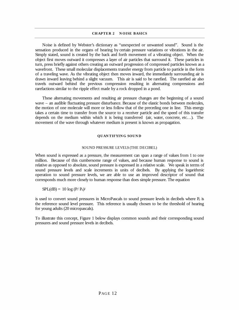
Noise is defined by Webster’s dictionary as “unexpected or unwanted sound”. Sound is the sensation produced in the organs of hearing by certain pressure variations or vibrations in the air. Simply stated, sound is created by the back and forth movement of a vibrating object. When the object first moves outward it compresses a layer of air particles that surround it. These particles in turn, press briefly against others creating an outward progression of compressed particles known as a wavefront. These small molecular displacements transfer energy from particle to particle in the form of a traveling wave. As the vibrating object then moves inward, the immediately surrounding air is drawn inward leaving behind a slight vacuum. This air is said to be rarefied. The rarefied air also travels outward behind the previous compression resulting in alternating compressions and rarefactions similar to the ripple effect made by a rock dropped in a pond.
These alternating movements and resulting air pressure changes are the beginning of a sound wave – an audible fluctuating pressure disturbance. Because of the elastic bonds between molecules, the motion of one molecule will more or less follow that of the preceding one in line. This energy takes a certain time to transfer from the source to a receiver particle and the speed of this transfer depends on the medium within which it is being transferred (air, water, concrete, etc…). The movement of the wave through whatever medium is present is known as propagation.
QUANTIFYING SOUND
SOUND PRESSURE LEVELS (THE DECIBEL)
When sound is expressed as a pressure, the measurement can span a range of values from 1 to one million. Because of this cumbersome range of values, and because human response to sound is relative as opposed to absolute, sound pressure is expressed in a relative scale. We speak in terms of sound pressure levels and scale increments in units of decibels. By applying the logarithmic operation to sound pressure levels, we are able to use an improved descriptor of sound that corresponds much more closely to human response than does simple pressure. The equation
SPL(dB) = 10 log (P/P0)2
is used to convert sound pressures in MicroPascals to sound pressure levels in decibels where Po is the reference sound level pressure. This reference is usually chosen to be the threshold of hearing for young adults (20 micropascals).
To illustrate this concept, Figure 1 below displays common sounds and their corresponding sound pressures and sound pressure levels in decibels.
Because the human ear does not respond to all pressures in complex sounds, noise measurement instruments are designed with “filters” which provide only measurements of sound pressure levels that the human ear may be sensitive to. This process is known as “weighting”. Figure 2 illustrates three such weighting systems.
PAGE 14
Figure 2 Frequency Responses for Sound Level Meter Weighting Chracteristics13
The A-scale curve corresponds roughly to the ear’s response in the range from about zero to 65 dB. The B-scale covers the range of nominally 65 to 85 dB while the C-scale, which is nearly linear, corresponds to the ear’s performance above 85 dB.
Studies show that when people make judgements of the “loudness” of a noise, their judgements correlate quite well with the A-scale sound levels of these noises. For this reason, A-weighting is applied to measurements and predictions for highway noise studies.
DESCRIBING SOUND
Because most sound levels fluctuate with time, a statistical descriptor must be used to describe the characteristics of the sound levels.
The Ldn descriptor is the A-weighted noise level averaged over a 24-hour period. Appropriate time-weightings are applied for the noise levels occurring in the daytime and nighttime periods. It was designed to improve on Leq by adding (linearly) a 10-dB correction penalty for nighttime noise intrusions to account for the increased annoyance during those hours. The Ldn descriptor is used by several federal agencies (EPA, HUD, FAA) to assess community noise environments and to set environmental noise standards.
Lmax is a simple descriptor that illustrates the highest sound level measured in a given time period. But because Lmax is limited in the information it provides, cumulative descriptors are better
PAGE 15
measures of the effects of sound. Cumulative descriptors better describe the random fluctuation in time of highway noise. L10 gives the dBA level that is exceeded only 10 percent of the time. Likewise, L50 gives the dBA level that is exceeded 50 percent of the time.
But these descriptors are limited in that they reflect the statistical nature of the noise time pattern. They do not provide a practical human understanding of noise levels. For this reason, Leq is used to describe highway noise. This “equivalent” noise level represents the level which, if held constant over the specified period of time, would yield the same amount of energy as the actual fluctuating noise. Thus, Leq is a more versatile descriptor than the percentile descriptors and is more easily understood by the average person.
THE THREE ASPECTS OF SOUND: SOURCE, PROPAGATION, RECEPTION
Sound is comprised of three inseparable aspects: the source, propagation, and the receiver. The source is the originator of the sound or the sound generator. Propagation is the process by which the sound moves from the source to the receiver and the receiver can be defined as any person or object in the path of the sound. All three of these aspects of sound must be present for noise to occur.
SOURCE
Sources can be described by the shape of the wave pattern they emit. A single parked automobile with its engine idling would be described as a point source. A source such as a large loudspeaker would emanate a planar shape of sound waves and many single vehicles traveling in a steady stream of traffic would be described as a line source. Different types of sources generate different types of sound wave spreading patterns. These patterns will be discussed in the next section
PROPOGATION
Propagation is the passage of sound energy or sound waves from the source to the receiver. Aspects of the transfer medium and the shape of the source itself, can affect the propagation of sound resulting in a change in energy at the receiver. Spreading patterns, the effects of shielding, ground shape and type, as well as atmospheric conditions can all effect the propagation of sound from source to receiver. These aspects with respect to highway sound propagation will be discussed here.
Spreading Effects
As sound waves move away from their source, be it point-, planar-, or line-shaped, they decrease in intensity. A point source creates a spherical spreading pattern that moves away from the source in all directions. A planar source would generate a plane of sound waves and a line source creates a cylindrical spreading pattern as the waves move away from the line in all directions. The sound generated by highway traffic is typically described as either point or line-shaped as illustrated in the previous examples. For this reason, we will focus on point and line sources in this discussion.
The intensity of the sound energy decreases as the distance away from the source increases. This spreading phenomenon can be estimated by the use of the following equation:
PAGE 16
I = W A Where: I = intensity W = sound power passing through Area A (time rate of sound energy release)
A = area through which the sound power passes
For a point source (spherical spreading pattern),
I = W . 4 π r2 For the line source (cylindrical spreading pattern),
I = W . 2 π r Where r = the distance from the source to the receiver.
Likewise the change in decibel level from the source to the receiver is also affected by the shape of the spreading pattern.
For a point source, the change in level is described as:
∆L = 10 log p12 p02
and for a line source, the change in level is described as:
∆L = 10 log p1 2 p0
where p0 is the source sound pressure level
and p1 is the receiver sound pressure level.
These equations show that under ideal conditions, for every doubling of distance from a point source, we lose 6 dBA. Similarly, for every doubling of distance from a line source, we lose 3 dBA due to the effects of spreading and the pattern of the sound wave propagation. But conditions are rarely ideal. Objects located between the source and receiver, ground conditions, and atmospheric conditions all affect the sound level intercepted by the receiver.
PAGE 17
Shielding Effects
Receptors of highway noise are rarely isolated houses or buildings situated on flat land with no obstructions between the highway and the receptor. Large trees, other buildings, rolling terrain, large signs, and fences are all examples of obstructions that must be considered when examining highway noise at a receptor.
When sound waves leave a highway source they often encounter obstructions before the wave reaches the receptor in question. A portion of the energy striking the broad surface of an object in the path of the propagating sound wave is transmitted through to radiate to the opposite side. The amount of energy lost in the passage is called transmission loss (TL) and depends primarily on the obstruction’s density. A portion will be absorbed into the obstruction. The amount is a function of the surface roughness and softness. Still another portion is “bent” around the edges of the object into the shadow zone behind it. This phenomenon is known as diffraction. When a wavefront strikes the edge of an object, many additional little “wavelets” are created there as thought the edge had become a new source. These wavelets combine to form a diffracted wave that propagates into the region behind the object. The remainder of the wavefront is reflected off the surface in a different direction.
These four aspects of shielding: transmission, absorption, diffraction, and reflection, must be understood in each case in order to predict the effects of highway noise.
Ground Effects
The two geometric spreading configurations considered in the previous discussion assume that there is no ground under the two sources. In reality, the two spreading patterns would be semi-spherical and semi-cylindrical if there were a flat ground below them. Since highway noise typically emanates from a source near the ground, we consider the effects of the ground’s surface as a reflector/absorber in the path of the sound waves. Experimental evidence shows that where sound from a highway (assuming a cylindrical source) propagates close to soft ground (plowed farmland, grass, crops) the most suitable drop-off rate is 4.5 dB instead of the 3 dBA outlined above. Likewise, measurements of individual vehicles (point source) have shown drop-off rates of 7.5 dB as opposed to 6. For hard surfaces such as concrete parking lots and paved areas, the 3 and 6 dB loss is accurate for a point and line source respectively.
These numbers assume the ground between the source and receiver is level terrain. Shielding effects must be considered in conjunction with hard and soft ground effects in the case of rolling or hilly terrain. A receiver that is located on a hill higher than the source will intercept less of the transmitted sound wave energy than a receiver on flat terrain or one that is at a lower elevation than the source. This correlation of effects due to hard/soft ground and rolling terrain add to the complexities of highway noise prediction.
Atmospheric Effects
Since air is the primary medium through which traffic noise is propagated, atmospheric effects can play a role in the change in intensity of sound energy between the source and the receiver. Precipitation, wind fluctuations, wind gradients (with altitude), temperature, temperature gradients (with altitude), and relative humidity are atmospheric factors to consider in the evaluation of sound transmission.
PAGE 18
According to the Federal Highway Administration’s “Highway Noise Fundamentals”, no noticeable effect on sound transmission would occur from a steady smooth flow of wind; however, wind speeds are slightly higher above the ground than at the ground and the resulting wind speed gradients tend to “bend” sound waves over large distances. Sound traveling with the wind is bent down to earth, while sound traveling against the wind is bent upward above the ground. There is little or no increase in sound levels due to the sound waves being bent down, but there can be noticeable reduction of sound levels ( sometimes up to 20-30 dBA) at relatively long distances (greater than a few hundred meters) when the sound waves are bent upward (for wind speeds of 15 to 35 kph). Irregular gusty winds provide fluctuations in sound transmission over large distances. Previously, it was thought that the net effect of these fluctuations may be an average reduction of a few decibels (4 – 6) per 100 m for gusty wind with speeds of 25 – 50 kph.[13]
With temperature inversions, the warm air above the surface bends the sound waves down to earth. These effects, previously thought to be negligible at short distances, can produce increase in sound levels at ground elevation at large distances (over 800 meters) for some geometries and thermal structures.
Previous highway noise prediction methods did not take temperature gradients or other atmospheric effects into account since their effects were not completely understood; however, recent research has shown that atmospheric effects on traffic noise levels can be significant even at close distances. Wind speeds parallel and vertical to the highway may become important at distances over 120 meters from the edge of pavement. Ray bending due to wind shear, turbulence, and temperature lapse rates may affect the noise levels received at distances as close as 100 meters.14 Studies currently being conducted may lead to inclusion of this parameter in future noise analysis.
One last consideration when accounting for atmospheric conditions is their affect on the behavior of motorists. Various forms of precipitation may cause a speed reduction in the traffic stream. Rain may tend to reduce highway noise slightly but the wet pavement surfaces can increase the high frequency content of tire noise thereby increasing the sound levels observed at the receiver. Conversely, snow can reduce the traffic speed while simultaneously providing a ground cover which can absorb some of the sound. These conditions must be considered when measuring highway noise for comparison with model-predicted results.
RECIEVER
In the case of human response to noise, receiver sensitivity becomes complicated by issues such as speech interference, annoyance, hearing loss, psychological and physiological effects, and even property depreciation.
Human sensitivity to sound is a function of the intensity or pressure of the propagating waves. Most sounds however are complex in that they contain a variety of simultaneously transmitted pressures and intensities. As previously discussed, the human ear is only sensitive to a certain range of these pressures. In an attempt to analyze only the sounds that are audible to human ears, we “weight” the frequency response to measure or report only those sounds that a human ear might be sensitive to. In this way, we measure only those sounds that correlate closely with human sensitivities. The effects of noise on humans has been divided into three categories:
n Activity interference
n General annoyance
PAGE 19
n Hearing loss
Studies show that the human hearing mechanism is far better at detecting relative differences in sound levels than absolute values. That is to say, one can more readily quantify increases and decreases of certain sound levels than identify the level of an isolated sound.
Similarly, the amount of the increase or decrease in noise level lends to our ability to audibly detect it. According to studies examined by the Federal Highway Administration, a person can just barely detect a sound level change of approximately one decibel for sounds in the mid-frequency range. When ordinary noises are heard, we can just detect level changes of 2-3 decibels. A 5 dB change is readily noticeable while a 10 dB change is judged by most people as a doubling or halving of the loudness. A 20 dB change is a dramatic change and a 40 dB change represents the difference between an faintly audible sound and a very loud sound.[13]
Activity interference
Speech communication and the quality of telephone usage are primary measures of activity interference. When communication is interrupted, noise levels have reached the point of annoyance. Assume two people were standing 1.5 m apart facing each other. If they are using a familiar vocabulary and speaking at normal voice levels, they could just carry on a conversation if the interfering noise level does not exceed 52 dBA at their ears for more than 50 % of the time or 58 dBA for more than 10% of the time.
Some studies have been done to establish the effects of highway noise on sleep interruption, but this document states that they are inconclusive and the issue needs further development.
General annoyance
While the activity interferences mentioned above certainly fall under the category of general annoyance, other less quantifiable nuisances may occur that are less specific than the interference with one activity. Interruption of listening to music, enjoying the quietness of meditative moments are both examples of general annoyance. In cases such as these, a smooth continuous flow of noise as with a fan is generally more acceptable than an impulsive noise or intermittent noise. As this relates to highway noise, a steady background hum of traffic noise is generally seen to be not as intrusive as an occasional single truck passing.
Hearing loss
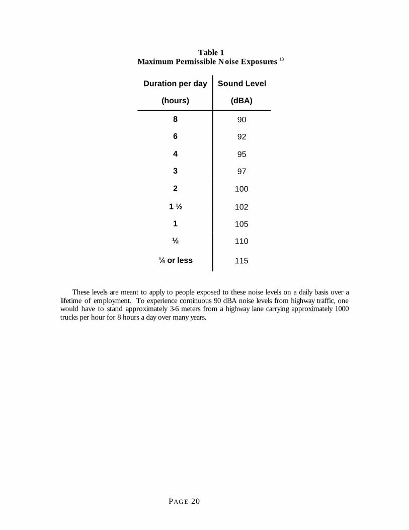
Studies have shown that long term exposure to high levels of noise can lead to hearing loss or hearing damage. In order to protect industrial workers from this type of injury, the Occupational Safety and Health Act of 1970 (OSHA) established maximum permissible noise exposures for persons working in high noise environments. Table 1 below outlines these limits.
PAGE 20
Table 1 Maximum Permissible Noise Exposures 13
Duration per day
(hours)
Sound Level
(dBA)
8 90
6 92
4 95
3 97
2 100
1 ½ 102
1 105
½ 110
¼ or less 115
These levels are meant to apply to people exposed to these noise levels on a daily basis over a
lifetime of employment. To experience continuous 90 dBA noise levels from highway traffic, one would have to stand approximately 3-6 meters from a highway lane carrying approximately 1000 trucks per hour for 8 hours a day over many years.
PAGE 21
CHAPTER 3 NOISE ANALYSIS AND MODELING REQUIREMENTS
REQUIREMENTS UNDER NEPA
An agency’s requirements under NEPA can be summarized into a three-step process.15 First, the agency must determine if NEPA applies to the proposal in question. NEPA applies if the proposal is subject to federal control and responsibility (often in the form of federal funding), and if the proposal is not “categorically excluded” from NEPA oversight. A categorical exclusion refers to a category of proposed actions which have been previously identified as having no significant effect on the environment such as highway shoulder widening or routine highway maintenance.
Second, the agency must determine whether an Environmental Impact Statement (EIS) or Environmental Assessment (EA) is required. According to the regulations, an EIS is required for “major Federal actions significantly affecting the quality of the human environment”16 The agency must determine if the proposal will have an effect on the human environment and if this effect is significant. The primary tool for making this determination is the EA. The environmental assessment is a cursory study of less depth than the EIS. It presents all the potential impacts of the proposal and the level of effect on the human environment.
The last step in the process is the preparation of an EIS or a Finding of No Significant Impact (FONSI). If the EA shows that the proposal may induce significant impacts, a detailed comprehensive study is conducted and outlined in the EIS. If no significant impacts are discovered, a FONSI is issued and the agency may proceed with its proposal.
Under the umbrella of NEPA, FHWA allows state highway departments to prepare EISs for jointly funded transportation projects. Among other issues, noise is a primary environmental concern when examining the effects of highway construction. In order to measure the impacts of highway noise, it must be monitored, measured, and predicted. FHWA has devised procedures for measuring and modeling highway noise so that each of the state highway departments may uniformly satisfy the requirements of NEPA when assessing proposals for federally funded transportation projects.
FHWA’S ABATEMENT PROCEDURES
FHWA’s noise abatement procedures are outlined in the Code of Federal Regulations (23CFR 772). These regulations define, among other things, the criteria that must be present for a noise impact to occur and the procedures for conducting a highway noise analysis.
According to FHWA’s criteria, a noise impact occurs when one of two conditions exist:
1) The projected noise levels approach or exceed the noise abatement criteria (NAC) shown in the following table, or
2) The projected noise levels substantially increase over the existing noise levels in an area.
FHWA’s Noise Abatement Criteria (NAC) are as follows:
Activity Category Leq (h) L10(h) Description of Activity Category
A 57
(Exterior)
60
(Exterior)
Lands on which serenity and quiet are of extraordinary significance and serve an important public need and where the preservation of those qualities is essential if the area is to continue to serve its intended purpose.
B 67
(Exterior)
70
(Exterior)
Picnic areas, recreation areas, playgrounds, active sports areas, parks, residences, motels, hotels, schools, churches, libraries, and hospitals
C 72
(Exterior)
75
(Exterior)
Developed lands, properties, or activities not included in Categories A or B above.
D -- -- Undeveloped lands
E 52
(Interior)
55
(Interior)
Residences, motels, hotels, public meeting rooms, schools, churches, libraries, hospitals, and auditoriums
* Either L10(h) or Leq(h) (but not both) may be used on a project.
FHWA does not define what constitutes a substantial increase over existing noise levels nor does the agency outline how close “approach” is. These parameters are left up to the individual states to determine and regulate accordingly.
The analysis of traffic noise impacts expected from highway construction must include the following steps for each alternative under detailed study:
1) Identification of existing activities, developed lands, and undeveloped lands for which development is planned, designed and programmed, which may be affected by traffic noise from the highway;
2) Prediction of traffic noise levels;
3) Determination of existing noise levels;
4) Determination of traffic noise impacts;
5) Examination and evaluation of alternative noise abatement measures for reducing or eliminating the noise impacts.2
If potential traffic noise impacts are identified, noise abatement is considered. If the abatement is found to be both reasonable and feasible, the measure is implemented. Similar to “approach” and
PAGE 23
“substantial”, the definitions of the terms “reasonable” and “feasible” are left up to the interpretation of the individual states.
MISSISSIPPI’S INTERP RETATION
The Mississippi DOT (MDOT) issued a Standard Operating Procedure to define and outline its policies and procedures for the consideration of highway traffic noise and noise abatement. The SOP states that MDOT will conduct a Highway Traffic Noise Study for each alternative of Type I (a new or expanded highway) projects under detailed study18. A summary of MDOT’s requirements for a highway traffic noise impact study are as follows:
1) Identification of existing and planned noise sensitive land uses – inventory of all activities that may be affected by highway noise
2) Determination of existing noise levels – will be made by measuring and/or predicting Leq noise levels for the traffic characteristics which yield the worst hourly traffic noise impact on a regular basis. At least one measurement for every 20 activities identified. Measurements are to be at least 15 minutes in duration with an ANSI Type 2 or better sound level meter.
3) Prediction of design year noise levels - Predictions must be made using a prediction method approved by FHWA.
4) Determination of traffic noise impacts – impacts will be determined by comparing existing and predicted design year noise levels with the Noise Abatement Criteria. Two types of impacts may occur:
a) “Approaches” is defined as 1dB below the NAC
b) “Substantially exceeds” is defined as 15 dB above the existing noise level
If either of these situations occurs, an impact is present.
5) Examination and evaluation of alternative noise abatement measures for reducing or eliminating noise impacts – noise abatement measures such as traffic management, changes in horizontal and vertical alignment, acquisition of property for buffer zones, noise insulation of public buildings, and construction of noise barriers will be considered
6) Preparation of noise study report – to be prepared if noise impact is expected to occur at any locations long the route of the proposed project. Sections to be included in the report are outlined.
The Mississippi DOT is an agency responsible for, among other things, the maintenance and construction of highways in a primarily rural state. Because of the sparse population along the majority of the construction projects in the state, no noise abatement measures have ever proven to be reasonable and feasible. Previously, noise and property acquisition considerations in the corridor location and alignment design phases have been adequate to prevent the need for noise abatement, but the growth of metropolitan areas along the gulf coast, the capitol city of Jackson, and the spreading metropolitan area of Memphis, TN may necessitate noise abatement construction in the near future.19
PAGE 24
CHAPTER 4 THE FHW A MODEL
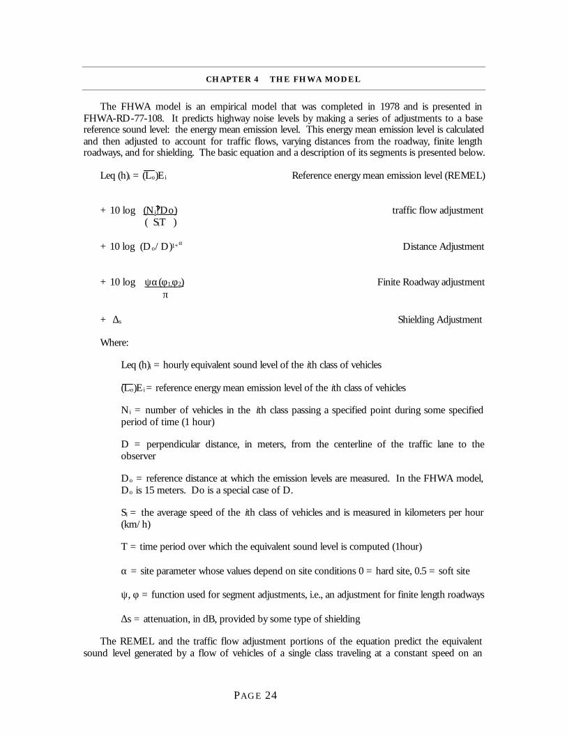
The FHWA model is an empirical model that was completed in 1978 and is presented in FHWA-RD-77-108. It predicts highway noise levels by making a series of adjustments to a base reference sound level: the energy mean emission level. This energy mean emission level is calculated and then adjusted to account for traffic flows, varying distances from the roadway, finite length roadways, and for shielding. The basic equation and a description of its segments is presented below.
Leq (h)i = (Lo)Ei Reference energy mean emission level (REMEL)
Leq (h)i = hourly equivalent sound level of the ith class of vehicles
(Lo)Ei = reference energy mean emission level of the ith class of vehicles
Ni = number of vehicles in the ith class passing a specified point during some specified period of time (1 hour)
D = perpendicular distance, in meters, from the centerline of the traffic lane to the observer
Do = reference distance at which the emission levels are measured. In the FHWA model, Do is 15 meters. Do is a special case of D.
Si = the average speed of the ith class of vehicles and is measured in kilometers per hour (km/h)
T = time period over which the equivalent sound level is computed (1hour)
α = site parameter whose values depend on site conditions 0 = hard site, 0.5 = soft site
ψ, φ = function used for segment adjustments, i.e., an adjustment for finite length roadways
∆s = attenuation, in dB, provided by some type of shielding
The REMEL and the traffic flow adjustment portions of the equation predict the equivalent sound level generated by a flow of vehicles of a single class traveling at a constant speed on an
PAGE 25
effectively infinite, flat roadway at a reference distance of 15 meters. Since this set of deal conditions rarely exists in reality, adjustments are then used to convert the reference level to a level that more accurately reflects actual conditions. The remaining sections of the equation make adjustments to this base assumption. Leq(h)i is calculated for each class of vehicles (autos, medium trucks, heavy trucks) and each of these values is added using log addition to arrive at the total Leq for the area. The following Figure outlines this process.
Figure 3 Flow Diagram of the Computational Sequence Used in the FHWA
Model20
REMELS
The reference energy mean emission levels used for the FHWA model were established in 1978 by the FHWA in the Four-State Noise Inventory. This study examined highway noise data from four states and was used to defined the REMELs in the FHWA model. This value L0 is defined by the FHWA model as the A-weighted, peak, pass-by noise level generated by a vehicle as measured by a microphone 1.5 meters above the ground at a perpendicular distance of 15 meters from the centerline of the traffic lane.
The FHWA model uses the following equations to predict the A-weighted national reference energy mean emission levels:
(Lo)EA = 38.1 log (S) – 2.4 Automobiles (Lo)EMT = 33.9 log (S) + 16.4 Medium Trucks (Lo)EHT = 24.6 log (S) + 38.5 Heavy Trucks
where S is the average vehicle speed in km/h. These levels were developed for cruise conditions on flat roadways with constant traffic moving at speeds between 50 and 100 km/h.
The Four-State Noise Inventory indicates that there are regional trends for REMELs. Different states obviously have different traffic conditions. For example, truck weight laws, average number of axles on large trucks, and recent trends toward larger two axle autos (sport utility vehicles) can all affect this base reference sound level. In 1993 the Florida Department of Transportation improved the REMELs used in their modeling program based on updated Florida traffic conditions. The upper speed limits were increased from 97 kph to 113 kph and the lower limit was reduced from 48 kph to 32 kph. Data collected more accurately reflected traffic conditions in the state of Florida. The result was improved accuracy in predicting the levels of traffic noise impacts.
REMEL Flow Adjustment
Distance Adjustment
Segment Adjustment
Shielding Adjustment
Predicted Sound Level
PAGE 26
DISTANCE
Since the REMELs are equivalent sound levels based on a distance of 15 meters, this value must be adjusted for receptors greater than 15 m away from the traffic source. α is the site parameter used to adjust for reflective and absorptive ground conditions. For α = 0, the site is assumed to be hard and the drop-off rate is 3dB per doubling of distance. For α = 0.5 the site is assumed to be soft and the drop-off rate is 4.5 dB per doubling of distance.
FINITE LENGTH ROADWAY ADJUSTMENTS
The Φ parameters are used to adjust for cases where the roadway is a finite segment. Segments can be to the left or right of the observer and may be of any length. Phi parameters of + and – 90 degrees are used when it is assumed that the roadway is of infinite length. Often this parameter is used to adjust the site model to account for large obstructions. Since the absorption parameter α is also used in this calculation, this segment of the equation can also be used to more accurately reflect a change in site ground conditions that occurs in the middle of the site.
SHIELDING
Shielding is taken into account by the factor ∆. Shielding can be provided by dense woods, rows of buildings, or any solid obstruction between the highway noise source and the receptor in question. This document describes the decibel reduction to be assumed given different varieties of shielding situations. Very dense foliage may reduce decibel levels by as much as 5 dBA for the first thirty meters and 5 dBA for the second 30 m but not more than 10 dBA total. Rows of houses are assumed to reduce levels by 3 dBA for 40-60% area covered and 5dBA for 65-90% area covered. Each additional row of houses from the noise source is assumed to receive a reduction of 1.5 dBA with a 10dBA cap on this reduction as well.
OTHER CONSIDERATIONS
ATMOSPHERIC ABSORPTION
Noise level changes due to temperature gradients, winds, and atmospheric absorption do occur but are ignored in the FHWA model. Attenuation due to wind and temperature gradients are ignored because conditions can vary drastically from site to site and because the attenuation they provide are not permanent anyway. Atmospheric absorption, absorption caused by water vapor, can affect readings, but is negligible in the short distances used for highway noise calculations.
LOW VOLUME ROADWAYS (ND/S < 40M/KM)
Experience has shown that measured noise levels and FHWA model predicted levels can differ drastically on low volume roadways. There are several reasons for this:
1) The reference energy mean emission levels that the model is based on was derived from average values of large samples of vehicles. Low volume roadways often do not contain the representative sample of auto traffic for the model to properly predict noise levels.
PAGE 27
2) The FHWA model assumes that the vehicles are evenly spaced on the roadway. When Leq is used as a descriptor, this issue is covered.
3) There is no assurance that the measured sound levels on low volume roadways adequately represent the average condition for the area. The average condition is what the model was designed to predict.
HIGH VOLUME ROADWAYS
High volume roadways can become a problem as density increases and volume inversion occurs. Volume inversion is a traffic phenomenon that occurs on heavily traveled roadways. As congestion increases, vehicles are forced to slow down, spacing decreases, and speeds decrease. This results in very high volumes but decreases in speeds. These conditions are most typical of urban and congested rural situations are also not reflected in the model design. Since the FHWA model isn’t accurate for very low and very high speeds, volume inversion can result in faulty noise level predictions.
EQUIVALENT LANE DISTANCE
As the number of traffic lanes to analyze increases, the difficulty of the modeling process increases. The equivalent lane distance was designed to simplify this process. Traffic is lumped without change in speed or operations assumptions onto an imaginary single late that yields approximately the same results as the more detailed analysis. The equivalent lane distance is the distance to one lane that is equivalent to actual conditions which may include several lanes as in the situation of a divided highway or two intersecting roads. This condition can be calculated according to the following equation:
DE = √(DN)(DF) Where:
DN = the perpendicular distance from observer to CL of near lane
DF = perpendicular distance from the observer to the centerline of the far lane.
FEATURES AND LIMITATIONS OF THE FHWA MODEL
The primary feature in the FHWA model’s favor is its simplicity of use coupled with accuracy for a large number of highway noise modeling applications, especially in primarily rural states such as Mississippi. The model requires input that is easily gathered in a short time period. Distances from receptor to roadway, traffic flows and predictions, and simple site parameters are fed into a complex set of equations either through a computer program such as STAMINA or a simple spreadsheet and desired output is almost instantaneous. Training for field personnel and analysts is not extensive. This simple input data and ease of operation translates into relatively inexpensive noise prediction.
The old FHWA model has three primary limitations. The first involves the emission levels used in the calculation of the base sound level. These emission levels are outdated and never applied equally to all states of the country even though all states are required to use them. Second, the model has a weakness in the area of shielding. Noise levels are not easily predicted in situations where dense foliage, building rows or other aspects of the landscape partially shield the receptor from the highway. Shielding has to be estimated by the noise analyst and simply subtracted from the overall predicted level. FHWA has provided “rule-of-thumb” shielding factors to use in different
PAGE 28
circumstances, but again, these don’t always yield accurate results in every situation. Finally, the old FHWA model doesn’t allow the analyst to accurately represent differing ground types and their affects on the predicted sound levels. Paved parking lots, sandy beaches, and baseball fields all affect the propagation of the sound and the amount that is absorbed by the ground before it reaches the receiver. The old model only allows for input of two types of ground surface: hard and soft. Often, conditions in the field are just not so simple.
VDOT’S EXCEL MODEL
The model used for comparisons in this paper was developed by Robert E. Gibson of the Environmental Division at the Virginia Department of Transportation (VDOT). This application of the FHWA model was designed by VDOT and approved by FHWA for use in 1987. It was originally intended to be used in the Air, Energy, and Noise Section for predicting noise levels in simple modeling applications but because of the its simplicity and accuracy, VDOT trained its district offices in noise modeling and they began using it to conduct complete EAs in the field offices freeing up the central office’s small environmental staff to concentrate on larger more complex projects.
The original VDOT application of the FHWA model was a LOTUS spreadsheet applying the basic algorithms in a simple, easy to input format. Revisions to the model were made in August of 1991 and March of 1993 and it was converted to EXCEL in August of 1997 with other minor improvements.
A copy of the input /output page is shown below.
PAGE 29
Figure 4 VDOT Model: Example Input/Output
Inputs are located in line 16 above and include: traffic volume in vehicles per hour, speed in MPH, percent trucks, lane width, number of lanes, distance from the receptor to the edge of pavement, left and right angle from the receptor to the end of roadway, factor for the ground type (0 for hard ground, 0.5 for soft ground), and the approximate percent grade of the roadway.
Most of these inputs can be gathered from a brief site visit and traffic data provided by DOT planning departments. The information is typed directly into the spreadsheet cell and the predicted sound level in decibels is calculated almost immediately and shown in the bottom right corner of the screen (cell L23 above). This page can then be printed out for recording purposes and the next data set input. Because of the speed of the calculation, the model is also simple to use for noise contour calculations which are required by many states for noise studies. Distances are input iteratively until the desired contour level appears in the “Grand Total” box.
The spreadsheet page shown above is applied to simple one-roadway scenarios. Seven other sheets in the EXCEL workbook are present that allow the user to input data from other roadways providing for modeling of more complex situations of up to 8 separate highways. For example, a receptor near a 4-lane highway would be modeled using the “NOISE2” spreadsheet and a receptor near a 4-lane highway intersecting a 2-lane local road would be modeled using the “NOISE3”
PAGE 30
spreadsheet and so on. Inputs are similar, in that the perpendicular distance from the roadway to the receptor is used in the calculation. Other inputs such as ground type and angle to the end of the roadway segment in question are also included for each of these additional roadways.
The primary difference between STAMINA 2.0 and the VDOT model is the coordinate system that is used in the application. STAMINA 2.0 uses an X,Y,Z Cartesian coordinate system to identify the location of roadways and receptors. The VDOT application of the FHWA model simplifies this process to X and Y plane only. Though STAMINA 2.0 is slightly more accurate21, other states including Mississippi regularly apply the model to simple rural projects with favorable results.
PAGE 31
CHAPTER 5 THE TNM MODEL
The Federal Highway Administration’s Traffic Noise Model® is an empirical model similar to its predecessors in that it computes a reference sound level and then makes a series of adjustments to produce a sound level prediction at a receiver. TNM is based on an X,Y,Z Cartesian coordinate system and is a computer program designed to run on a personal computer. The basic model can be described by the following equation:
LAeq1h = ELI + Atraff(i) + Ad + As
Where EL represents the vehicle noise emission level (REMEL) for the ith vehicle type,
Atraff(i) represents the adjustment for traffic flow, the volume and speed for the ith vehicle type
Ad represents the adjustment factor for distance between the roadway and receiver and for the length of the roadway
As represents the adjustment for all shielding and ground effects between the roadway and the receiver 12
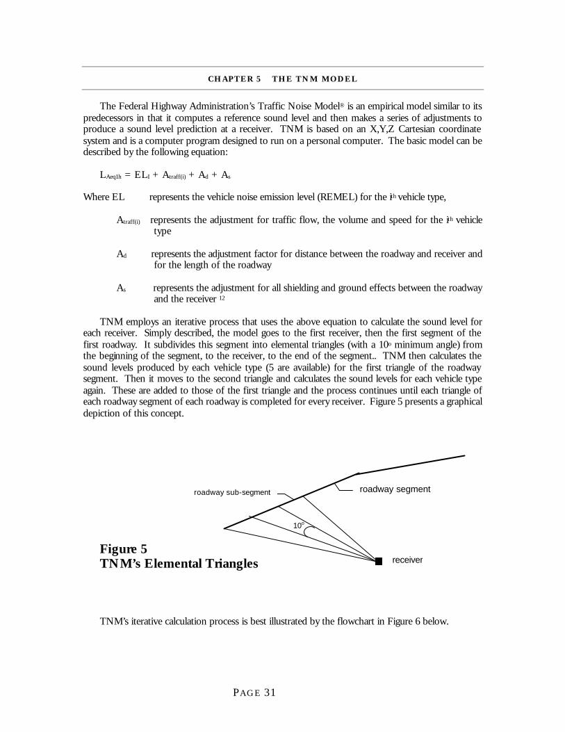
TNM employs an iterative process that uses the above equation to calculate the sound level for each receiver. Simply described, the model goes to the first receiver, then the first segment of the first roadway. It subdivides this segment into elemental triangles (with a 10o minimum angle) from the beginning of the segment, to the receiver, to the end of the segment.. TNM then calculates the sound levels produced by each vehicle type (5 are available) for the first triangle of the roadway segment. Then it moves to the second triangle and calculates the sound levels for each vehicle type again. These are added to those of the first triangle and the process continues until each triangle of each roadway segment of each roadway is completed for every receiver. Figure 5 presents a graphical depiction of this concept.
Figure 5 TNM’s Elemental Triangles
TNM’s iterative calculation process is best illustrated by the flowchart in Figure 6 below.
10o
receiver
roadway segment roadway sub-segment
PAGE 32
Figure 6 High-Level Flow Chart of TNM Calculations12
Bas
ic M
odel
Equ
atio
n
Begin with entire geometry
Iterate over receivers
Iterate over roadways
Set speed computation flag for all affected vehicles
Iterate over roadway segments
Subdivide segment into elemental triangles if necessary
Iterate over elemental triangles
Iterate over vehicle types
Compute speed for triangle if necessary , Clear speed flags if appropriate
Compute vehicle emission level by sub-source height
Compute A traff (adjustment for volume and speed)
Compute Ad (adjustment for distance and length of the roadway
Compute As (adjustment for shielding and ground effects)
Compute and store LAeq1hr, Ldn, or Lden at receiver for this vehicle type and triangle
Next receiver
Set speed computation flag for heavy trucks
Determine if traffic control devices are
present
Y
YDetermine if road segment is upgrade ≥ 1.5%
Next roadway and clear all speed flags
Next vehicle type
Next elemental triangle
Next roadway segment
PAGE 33
Inputs into TNM can be made through several mediums. TNM accepts STAMINA 2.0 files directly though some minor editing is required first. Also, CADD DXF files can be called into TNM in two separate ways. The graphic file can be imported as a background image to allow the user to perform “heads-up” digitizing on the screen as a method of creating TNM objects (roadways, receivers, ground lines) or the file can be imported directly as a TNM object set. This method, however is a very lengthy process and often results in an enormous amount of editing after the file is completely imported. Finally, TNM objects may be input from plan sheets using a digitizing board and puck. The plan sheet is referenced in the model and the roadway, terrain features, and receivers are digitized by tracing them with the puck. This method seems to be preferred by most noise analysts using TNM.
The following discussion is a description of the four elements of the fundamental equation upon which TNM is based.
NOISE EMISSION LEVELS
The first element of the model is labeled EL, noise emission levels which are based on the old REMELs (Reference Energy Mean Emission Levels). In the fundamental equation, this standard base number is calculated for each vehicle type and then adjusted according to the specific site parameters input into the model. Data from vehicle pass-by tests of approximately 6000 vehicles in 9 states was gathered to develop these revised emission levels. The database was developed for automobiles, medium and heavy trucks, buses, and motorcycles and was gathered for vehicles cruising, accelerating, idling, and for vehicles on grades. In addition, vehicles traveling on different pavement types were examined: densely graded asphalt, open graded asphalt and Portland cement concrete.
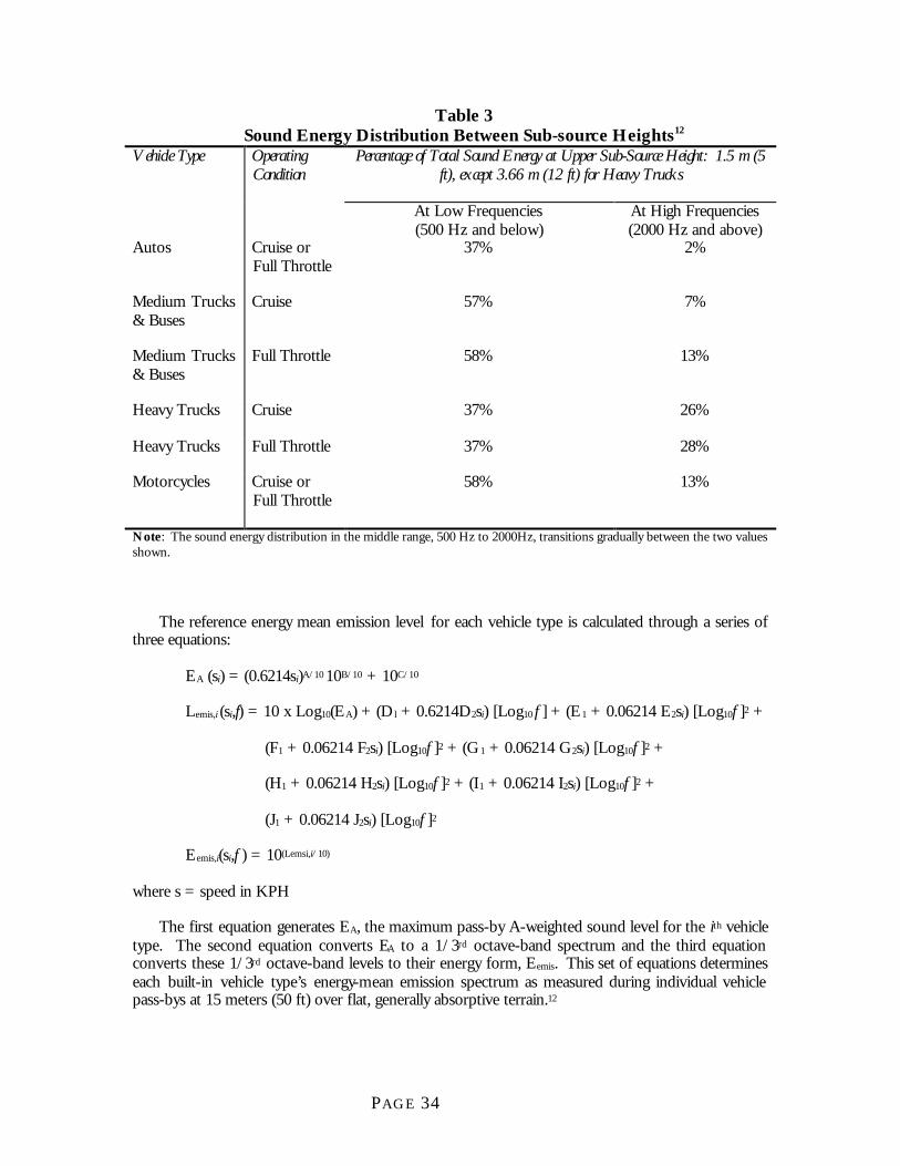
Additional research led to the development of two sub-source heights for each vehicle and three sub-source heights for heavy truck. Zero represents the noise from tires interacting with the pavement, 1.5 meters (5 feet) represents the noise contributed by the engine and 3.66 meters (12 ft) is reserved for heavy truck exhaust. This study determined the ratio of sound energy distributed at the lower and upper heights as a function of frequency, vehicle type, and throttle condition. The total sound energy distribution from the upper sub-source height is presented below in Table 3.
PAGE 34
Table 3 Sound Energy Distribution Between Sub-source Heights12
Percentage of Total Sound Energy at Upper Sub-Source Height: 1.5 m (5 ft), except 3.66 m (12 ft) for Heavy Trucks
Vehicle Type Operating Condition
At Low Frequencies (500 Hz and below)
At High Frequencies (2000 Hz and above)
Autos Cruise or Full Throttle
37% 2%
Medium Trucks & Buses
Cruise 57% 7%
Medium Trucks & Buses
Full Throttle 58% 13%
Heavy Trucks Cruise 37% 26%
Heavy Trucks Full Throttle 37% 28%
Motorcycles Cruise or Full Throttle
58% 13%
Note: The sound energy distribution in the middle range, 500 Hz to 2000Hz, transitions gradually between the two values shown.
The reference energy mean emission level for each vehicle type is calculated through a series of three equations:
EA (si) = (0.6214si)A/10 10B/10 + 10C/10
Lemis,i (si,f) = 10 x Log10(EA) + (D l + 0.6214D2si) [Log10 f ] + (E1 + 0.06214 E2si) [Log10f ]2 +
The first equation generates EA, the maximum pass-by A-weighted sound level for the ith vehicle type. The second equation converts EA to a 1/3rd octave-band spectrum and the third equation converts these 1/3rd octave-band levels to their energy form, Eemis. This set of equations determines each built-in vehicle type’s energy-mean emission spectrum as measured during individual vehicle pass-bys at 15 meters (50 ft) over flat, generally absorptive terrain.12
PAGE 35
FHWA policy allows for states to develop their own REMELs for input into the old model and TNM is designed to provide this condition.
TRAFFIC FLOW ADJUSTM ENT
TNM adjusts the reference level for traffic flow by taking into account traffic volume (number of vehicles per hour) and speed. The adjustment is calculated separately for each vehicle type:
Atraff(i) = 10 x Log10 (Vi\Si) – 13.2 dB
where Vi is the vehicle volume in vehicles per hour and
Si is the vehicle speed in kilometers per hour.
Input speeds are used directly in the calculations under all but two circumstances:
1. Whenever truck speeds are reduced by the presence of upgrades
2. Whenever traffic speeds are reduced by the presence of traffic control devices such as stop signs, entrance ramps, or traffic signals.
For up-grades, TNM starts computing heavy-truck speeds where the upgrade equals 1.5% or more. TNM computes speeds at the traffic control device itself. Traffic-control devices abruptly reduce speeds to the device’s “speed constraint” input by the user except in the case of signals where only the portion of the traffic stopped to the red phase is affected. TNM stops computing speeds when the vehicles accelerate back up to the user’s input speed or when the vehicle comes to the end of the current TNM roadway. In this manner, computations for each roadway are completely independent of speeds on connecting roadways.
DISTANCE ADJUSTMENT
Since the reference mean energy level were calculated for a receptor 50 feet from the roadway, TNM adjusts this number for the actual distance to the input receptors. This is done through the following equation:
Ad = 10 x Log10 15 α dB d 180
where d is the perpendicular distance to the line representing the roadway segment and
α is the angle subtended by the elemental roadway segment in degrees.
TNM calculates the distances based on X and Y coordinates input by the user. This adjustment is the same for all vehicle types, source heights and frequencies.
SHIELDING AND GROUND EFFECTS
Unlike the distance adjustment which acted in the X,Y plane only, shielding and ground effects are three dimensional in nature. Ground points are intrinsically part of the roadway definition in the model but are also an input with the receivers and other effects such as tree zones, terrain lines and
PAGE 36
building rows. Terrain lines can be input into the model by graphically drawing them in or by digitizing them off plan sheets. These lines define ground segments in which reflections can occur.
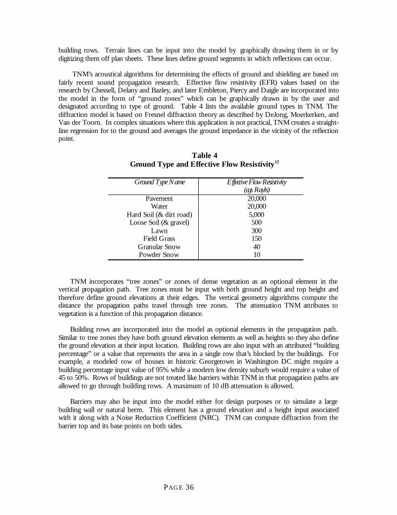
TNM’s acoustical algorithms for determining the effects of ground and shielding are based on fairly recent sound propagation research. Effective flow resistivity (EFR) values based on the research by Chessell, Delany and Bazley, and later Embleton, Piercy and Daigle are incorporated into the model in the form of “ground zones” which can be graphically drawn in by the user and designated according to type of ground. Table 4 lists the available ground types in TNM. The diffraction model is based on Fresnel diffraction theory as described by DeJong, Moerkerken, and Van der Toorn. In complex situations where this application is not practical, TNM creates a straight-line regression for to the ground and averages the ground impedance in the vicinity of the reflection point.
Table 4 Ground Type and Effective Flow Resistivity12
Ground Type Name Effective Flow Resistivity
(cgs Rayls) Pavement 20,000
Water 20,000 Hard Soil (& dirt road) 5,000 Loose Soil (& gravel) 500
Lawn 300 Field Grass 150
Granular Snow 40 Powder Snow 10
TNM incorporates “tree zones” or zones of dense vegetation as an optional element in the vertical propagation path. Tree zones must be input with both ground height and top height and therefore define ground elevations at their edges. The vertical geometry algorithms compute the distance the propagation paths travel through tree zones. The attenuation TNM attributes to vegetation is a function of this propagation distance.
Building rows are incorporated into the model as optional elements in the propagation path. Similar to tree zones they have both ground elevation elements as well as heights so they also define the ground elevation at their input location. Building rows are also input with an attributed “building percentage” or a value that represents the area in a single row that’s blocked by the buildings. For example, a modeled row of houses in historic Georgetown in Washington DC might require a building percentage input value of 95% while a modern low density suburb would require a value of 45 to 50%. Rows of buildings are not treated like barriers within TNM in that propagation paths are allowed to go through building rows. A maximum of 10 dB attenuation is allowed.
Barriers may also be input into the model either for design purposes or to simulate a large building wall or natural berm. This element has a ground elevation and a height input associated with it along with a Noise Reduction Coefficient (NRC). TNM can compute diffraction from the barrier top and its base points on both sides.
PAGE 37
FEATURES AND LIMITATIONS
TNM’s primary feature is it’s graphic user interface. Often with the old STAMINA model, inputs were made “blind”. XYZ coordinate files had to be input into the model without a graphic depiction of the input. This was cumbersome and created an atmosphere for frequent input errors. TNM however, allows the analyst to visually check each input as it is created. Cartesian coordinates may be typed in directly for roadway, receiver, or other objects or they may be graphically created.
As previously discussed, these graphic objects may be brought in to TNM through a number of mediums but all have limitations. Importing TNM objects through CADD-created DXF files can take hours and still require much editing after the import process is complete. Using a digitizer to create roadway and receiver objects is simpler but requires the appropriate hardware to interface with the model. Presently the software only supports a Calcomp digitizer tablet which may or may not be available to all noise analysts. The work presented in this paper was completed by importing a DXF file as a background image and creating the objects graphically directly over the image. This too, was time consuming since the graphics program regenerates the entire image every time a dialog box is opened or other change is made to the screen. Approximately ¼ of the entire modeling time was spent waiting on regenerating backgrounds.
Unlike the old model which only predicted L10 and Leq noise levels, TNM computes Ldn and Lden as well. Ldn is the day-night average sound level and Lden is the Community Noise Equivalent Level (CNEL) where “den” stands for day/evening/night. These sound levels are averages similar to the Leq level, but as discussed in Chapter 2, they incorporate a correction penalty for nighttime noise. Inclusion of these descriptors into the TNM model was made in order to create better communication between Metropolitan Planning Agencies and federal agencies, specifically the FAA, who currently use these measures to quantify noise.
Another advantage of TNM is its apparent ability to accurately model interrupted flow facilities. Previously, the only way to model this scenario was to modify the cruise speeds needed for input into the old model. This could be done by “calibrating” the model using field-collected samples or by a method developed by Wayson and Bowlby in 1990. This research presented the concept of a Zone of Influence which is used to represent stretches of road on which acceleration or deceleration occurs. In these zones, sound levels are assumed to vary form cruise condition levels. Two series of equivalent constant speeds were developed that permitted STAMINA to calculate the desired noise level difference relative to the cruise condition.22 This concept is built directly into the TNM model. Through the complex speed calculations discussed previously in the “Traffic Adjustment” section of this chapter, TNM can reduce decibel levels due to changing speeds at stop-signs, entrance and exit ramps, as well as traffic signal situations reducing the level of judgement required of the noise modeler.
According to the cursory information that is available on comparisons between TNM and STAMINA/OPTIMA, TNM seems to provide better barrier designs. Noise walls designed through TNM are for the most part smaller in area than those designed using OPTIMA. One of the primary reasons for this is TNM’s ability to incorporate shielding of traffic noise from the roadway itself. Highways on fill typically provide some shielding through land widths and shoulders which was not taken into account in the previous noise prediction models. This, along with the better ground attenuation parameters in TNM seem to be reducing the height of walls required for decibel reduction.
The main disadvantage of TNM is its run-time. While the capabilities of the VDOT version of the old FHWA model are limited, results are virtually instantaneous. Depending on the complexity of the terrain and ground surface, a simple five mile segment of a 4-lane highway with 10 receptors
PAGE 38
along it can take anywhere from a couple of hours to an entire day to run in TNM. Presently, TNM considers all roadway segments in the model for each receiver. This can create enormous amounts of calculations for complex runs that have multiple numbers of roadway segments or receivers and is the primary reason TNM takes so long to run. Future plans for the model include a function that would allow the program to estimate receiver effects from only the roadway segments that actually contribute to it..23 This should decrease the run-time significantly.
The initial release of TNM (Version 1.0) had some algorithm complications that caused the model to create a “floating point” error just prior to crashing the computer. TNM was designed to operate on an 8-bit system under the conception that many state agencies that might be using the model may not have upgraded to the newer 16-bit Windows operating systems. Input of large coordinate numbers in describing the TNM objects created problems with this 8-bit limitation of the model. Though this “bug” was eradicated with the TNM version 1.0a patch, many inconsistencies similar to this are still present in the model.
PAGE 39
P A R T I I
M I S S I S S I P P I S T A T E R O U T E 1 5 C A S E S T U D Y
PAGE 40
CHAPTER 6 INTRODUCTION AND DESCRIPTION OF THE PROJECT
INTRODUCTION
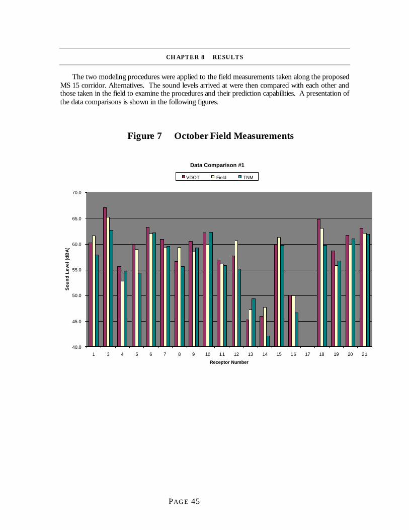
In August of 1999, the firm of Parsons Brinckerhoff contracted with the Mississippi Department of Transportation to perform and Environmental Assessment of the Mississippi state route 15 project from Pontotoc to Walnut, Mississippi. This environmental assessment was initially to be completed before the March 2000 deadline for transfer to TNM as the recommended model for highway noise study; therefore, predictions were calculated using the old FHWA model. With a total corridor length of almost 70 miles, the project has almost 1000 noise receptors along its four “build” alternatives.
As part of the noise study, field measurements were taken at 32 locations along the existing two lane facility. For this paper, the existing noise levels at these receptors were also modeled using the TNM method. A comparison of the results is presented here.
PROJECT AREA
This project is located in Northeast Mississippi approximately 20 miles west of Tupelo and 80 miles southeast of Memphis. The proposed highway goes through the urban areas of New Albany (pop. 6775) and Ripley (pop. 5371)24 and the towns of Blue Mountain and Falkner, as well as several small communities. The area is primarily rural with commercial activity situated in the urban areas. Farming is the primary industry of the region with some industrial facilities sporadically located in the small towns.
State Route 15 is described by the mayor of Ripley as “the longest 2-lane road in the state of Mississippi” because it traverses the state from the Tennessee state line to the Gulf of Mexico as a two-lane facility. This has previously been of little consequence since, with the exceptions of Laurel and Biloxi, all the cities along the route have populations of less than 7000. But with New Albany’s thriving Main Street program and it’s close proximity to Tupelo, its arterials are becoming almost impassable during peak hours. Similarly, the city of Ripley is growing and its economic development leaders desire better access to the cities of Tupelo and Memphis like New Albany, its southern neighbor.
ALTERNATIVES DESCRIPTI ON
The project is part of Phase IV of the 1987 Four-Lane Highway Program which was designed to be an economic development tool by the DOT and Mississippi State Legislature. The section of State Route 15 included in this study is approximately 48 miles long and spans three counties: Pontotoc, Union, and Tippah. SR 15 has been designated by MDOT as a Principal Arterial within the urban limits of New Albany and Ripley and a Minor Arterial outside these limits.25
The project alternatives are described here as they are positioned at the time of this writing and are shown in detail in Appendix B. The environmental assessment, as required by NEPA, refers to the four separate alternatives, but for the sake of this discussion we will describe the segments of the project. The project begins just north of the city of Pontotoc at SR 6 and continues northward paralleling the existing two-lane highway 125 ft west of the existing lanes. Access section is to be controlled by permit. That is, all current local roads and driveways will be accessible from the new highway.
PAGE 41
Two alternative locations are presented to serve the city of New Albany. The segment shown passing through the city is proposed as a five-lane curb and gutter section for which right-of-way was purchased almost 20 years ago. The second New Albany segment is a bypass to the east of the city which would be a divided highway with two sets of lanes 88 ft from centerline to centerline. Access to this alternative is to be limited.
The alignment continues north, paralleling the existing route 125 ft to the east due to the proximity of the Kansas City – Southern Railroad facility on the west side of the highway. Access to this segment, similar to the southern segment, will be allowed by permit and all existing access will be provided to the new route.
The town of Blue Mountain is then bypassed to the east beginning at the historic Rainey Plantation. The alternatives then split to propose two bypasses of the city of Ripley, east and west. These alignments are to consist of two sets of lanes, 88 ft from centerline to centerline, with partial control of access.
The alternatives converge again just south of the town of Falkner and parallel the existing facility 125 ft to the west to avoid conflict with the Kansas City – Southern Railroad as well as Falkner High School both located on the east side of the existing highway.
PAGE 42
CHAPTER 7 METHODOLOGIES
DATA COLLECTION
The data collection process began with the acquisition of aerial photography for the project corridor. These documents were provided at a scale of 1” = 500’ by the Mississippi Department of Transportation and were scanned into electronic images for use in Microstation Decartes. Project corridor alignments were designed using MDOT’s recommended locations and noise sensitive receptors were cursorily identified. These receptors were then field verified and their land uses noted on the photographs so that noise levels and noise level increases could be measured against the proper NAC.
FHWA and MDOT procedures were followed in conducting the field noise measurement for this project.26 Fifteen-minute Leq noise readings were taken at receptor locations while simultaneously counting traffic separated into auto, medium, and heavy trucks during the PM peak (3:30 to 6:00). Site selection was based on location to the corridor and an attempt was made to choose sites that would be modeled easily while providing a representative noise sample for surrounding receivers. Sites that were relatively flat with no obstructions were chosen and a priority was given to sensitive receptors such as cemeteries, churches and schools. An attempt was made to include “hard” sites in the readings for purposes of this comparison, but those sites are typically commercial in nature and tend to have a large amount of business traffic during peak hours. Several suitable locations were identified, but most of the measurements are located in areas of “soft” site predictions or “lawn”-type TNM ground zones.
A total of 36 field readings were taken in two different trips. Not all of this data was used in the comparisons presented in this paper since several of the readings were at receptors located along rural roads with no traffic at all. These readings were required in order to estimate the noise level increase after the proposed facility is built but they were not used in this comparison since the existing level could not be modeled.
Data was gathered in two separate site visits using two different sound level analyzers. The first site visit was conducted in mid-October of 1999. Twenty-one noise readings were taken at various locations along the project corridor (shown on the project alternatives maps located in Appendix B). These readings were taken with a Quest 8000 sound level analyzer. This monitor is a ANSI Type II meter which meets the requirements of both FHWA and Mississippi DOT; however, the instrument had a tendency to lose its calibration to within 0.5 to 0.7 dBA while in transit between noise sites. It also did not have an easily programmable internal clock that would allow it to self-time during the 15 minute intervals so hand-timing with a separate stop-watch was required during the reading process. For these reasons, among several others, a different noise meter was used for the second field trip measurements. This instrument was a Metrosonics dB8030, also an ANSI Type II meter, and was much better suited for highway noise measurement. The remaining sixteen readings were taken on the second field trip in mid-November using this monitor.
MODELING
VDOT SPREADSHEET
Modeling of existing conditions with the VDOT spreadsheet took approximately 4 hours and most of this time was spent modifying the spreadsheet to allow multiple row receptor input (see
PAGE 43
Appendix C for modified spreadsheet). The work was done using an EXCEL spreadsheet on a 120MHz Pentium with a 15” monitor running under Windows 98.
Traffic volumes were converted from the 15 minute field measurements to an hourly volume by multiplying them by 4 and uniform speeds were estimated based on experience and notes from the field. Phi angles of –90 and +90 were used in all but one location since receptors were chosen for their unobstructed view of the roadway. Several hard sites were modeled (alpha value of 0.0) and only one receptor had a roadway grade of 3.0 or greater. Since the existing condition was the only scenario modeled for this comparison, 2 twelve foot lanes were modeled for every receptor.
TNM
The TNM modeling process took approximately 25 hours, one-quarter of which was spent waiting on the computer to regenerate the DXF background over and over. This work was done on a 266 MHz Pentium II with dual processors and dual 17”monitors. Time was not available to test the TNM runs on other computers to see if the dual processors or a higher clockspeed would make a difference in the run-time or regen-time but comparison with similar runs on slower machines during training leads me to believe that clockspeed makes a significant difference in these parameters.
As previously discussed, for the purpose of this study, TNM objects were created by importing a DXF file into the model as a background and “heads-up” digitizing the roadways and receptor locations. Z-coordinates for these elements were estimated using USGS Quad maps by visually locating changes in elevation and inputting the correct values into the roadway and receptor segments. Similarly, terrain lines that had the potential to substantially effect sound levels at the receiver were estimated from the Quad sheets and graphically drawn into the model. This method of elevation input was painstaking, to say the least. Tablet digitizing might be a more accurate and less time consuming method, however, care must be taken in that process to minimize the number of input elements since every extra coordinate exponentially increases TNM’s run-time. Where hard sites were present, ground zones of the appropriate size were also drawn into the model using field sketches and areal photographs. A careful attempt was made to input receivers at distances very similar to those used in the VDOT model. Input of the receivers was done graphically also, but locations should be within ± 5 ft.
Since the project corridor is almost 50 miles long and the measurements were so far apart, each receptor, with a few exceptions, was modeled separately. In a typical EA noise study, this would not be feasible since the analyst would be modeling all potential receptors and they would likely be spaced closer together. This would probably increase the actual model run-time significantly. Because the receivers were modeled one at a time, the DXF background had to be re-imported and re-registered for each run. This also was painstaking and absorbed 15 to 20 minutes or so per run. Some problems were experienced when the DXF background “disappeared” after the “show/hide dxf” was activated. It was also noted that if an object was entered before the DXF was registered, the background converted to the new coordinate system whereas the object remained at its previous coordinates. This often made location of the background difficult since the “full view” command then had a huge area to cover, reducing the background to a microscopic orange dot.
Formatting the view for printing was also time-consuming since the DXF background regenerated every time the print-preview was activated. TNM runs and print-outs of the results are located in Appendix D. Receptors are colored and their corresponding numbers are sketched in by hand. The roadway element modeled is outlined in pencil. Since all line widths are the same, differentiation between the background and the objects is virtually impossible once the file is printed. Also the receptor and roadway labels do not scale up or down, so in this application they were too
PAGE 44
small to be legible. This was very inconvenient when viewing the roadway profiles since point numbers had to be identified by double-clicking the element and then viewing the input boxes.
PAGE 45
CHAPTER 8 RESULTS
The two modeling procedures were applied to the field measurements taken along the proposed MS 15 corridor. Alternatives. The sound levels arrived at were then compared with each other and those taken in the field to examine the procedures and their prediction capabilities. A presentation of the data comparisons is shown in the following figures.
A cursory examination of these results seems to imply that both TNM and the VDOT model overpredict noise levels in almost half the situations. Of the 32 receptors presented, 15 were over predicted by both TNM and the VDOT model. For 7 of the receptors, both models underpredicted. In 6 situations, the VDOT model overpredicted and TNM underpredicted and in 2 instances TNM overpredicted and VDOT underpredicted. In summary, the VDOT model overpredicted at a total of 21 receptors and TNM overpredicted at 17 receptors. This is consistent with the cursory findings that TNM does a better job at estimating the decibel reduction achieved due to shielding from the roadway and better ground absorption.
An interview with Robert Gibson, developer of the VDOT model, yielded the information that VDOT has observed a relationship between the difference in TNM and STAMINA predictions and distance from the receiver to the roadway. Mr. Gibson stated that he had compared TNM predictions to STAMINA predictions for 7 projects now and at distances close to the road, TNM predicts higher values than STAMINA. At approximately 200 feet, the models yield about the same results and at distances greater than 200 feet, STAMINA predicts higher values.
An attempt was made to investigate this relationship with regard to the VDOT model predictions. Figure 9 shows the differences in sound level predictions between the two models plotted with distance. This graph seems to indicate that for distances less than 75 to 100 feet, the two models equally yield high or low predictions but for distances greater than 75 feet, the VDOT
model consistently predicts higher than TNM. While 32 data points is not really adequate to make this assumption, these results would lead us to believe that the VDOT model is even more conservative than TNM or STAMINA. Also, more measurements of receptors at distances greater than 200 ft would help determine if this relationship is valid.
Figure 9 VDOT Vs TNM Predictions
In an attempt to examine both models’ ability to predict accurately, differences between predicted values and measured values were also plotted against distance. This comparison yielded the following results.
VDOT Model Predictions - TNM Predictions
-6.0
-4.0
-2.0
0.0
2.0
4.0
6.0
0 50 100 150 200 250 300 350
Distance From Roadway to Receptor (ft)
Dec
ibel
Dif
fere
nce
PAGE 48
Figure 10 VDOT Predictions
This figure seems to indicate that for 50 feet or less, the VDOT model is overpredicting and for distances of 50 feet to 150 feet, the model is underpredicting. An adequate amount of data is not available to make this determination for distances greater than 150 feet.
Measured Values - VDOT Model Predicted Values
-6.0
-4.0
-2.0
0.0
2.0
4.0
6.0
0 50 100 150 200 250 300 350
Distance from Roadway to Receptor (ft)
So
un
d L
evel
Dif
fere
nce
(d
BA
)
PAGE 49
Figure 11 TNM Predictions
The TNM model seems to equally overpredict and underpredict at distances less than 150 feet though the overpredicted values scatter almost 2 decibels further than the underpredicted values. Overall, for these short distances, the VDOT model only missed the field measurement by over 3 decibels three times whereas the TNM model missed the field measurement by this amount 5 times.
An attempt was made to see if these results were affected by the two different field noise analyzers. The previous figures were graphed with the Quest measurements as squares and the Metrosonics Measurements at triangles. The following figures are the results of this comparison.
Measured Values - TNM Predictions
-6.0
-4.0
-2.0
0.0
2.0
4.0
6.0
0 50 100 150 200 250 300 350
Distance From Roadway to Receptor (ft)
Sou
nd L
evel
Diff
eren
ce (
dBA
)
PAGE 50
Figure 12 VDOT Meter Comparison
In this graph the triangle data points are present both above and below the 0 error line indicating that the prediction errors were evenly dispersed between the Metrosonics meter and the Quest meter.
Noise Analyzer Comparison
-6.0
-4.0
-2.0
0.0
2.0
4.0
6.0
0 50 100 150 200 250 300 350
Distance from Roadway to Receptor (ft)
So
un
d L
evel
Dif
fere
nce
(d
BA
)M
easu
rem
ent
- V
DO
T m
od
el P
red
icti
on
s
Quest Field Measurement Metrosonics Field Measurement
PAGE 51
Figure 13 TNM Meter Comparison
A graph of the same results for the TNM model, however, shows the Metrosonics measurements as being closer to the 0 error line, an indication that this meter may be more accurate and that the change in noise meters may possibly have affected the outcome of these results.
Noise Analyzer Comparison
-6.0
-4.0
-2.0
0.0
2.0
4.0
6.0
0 50 100 150 200 250 300 350
Distance from Roadway to Receptor (ft)
Sou
nd L
evel
Diff
eren
ce (
dBA
)M
easu
rem
ent
- TN
M P
redi
ctio
n
Quest Field Measurements Metrosonics Field Measurements
PAGE 52
P A R T I I I
I M P L I C A T I O N S O F T H E N E W M O D E L
PAGE 53
CHAPTER 9 PROJECT LEVEL IMPLICATIONS
Many of the factors that affect the noise analyst’s use of TNM have been previously discussed, but the implications they will have on each individual project’s cost and schedule will have far reaching effects. In order to compare the rise in noise study cost due to FHWA’s change to TNM, an estimate of the complete Mississippi State Route 15 noise study as provided by Parsons Brinckerhoff (utilizing the VDOT model for noise prediction) was compared with an estimate of the same project as modeled in TNM. These two budgets are presented below.
Figure 14 Budget Estimate for MS 15 Project Using the VDOT Model
VDOT Hour Worksheet
Mississippi Department of Transportation 95-0022-00-005-10 / 102935901000 Date: 1-Dec-99SR 15 Fr Pontotoc to Walnut
Parsons Brinckerhoff Pontotoc, Union , Tippah Counties
Project: SR 15 from Pontotoc to Walnut MDOT No: 95-0022-00-005-10 / 102935901000Noise Study
Direct CostsPersonnel Est Hours Rate/Hr Cost ($) TotalsProject Manager 4 $40.00 $160Senior Planner 0 $27.00 $0Env. Planner/ Engineer 176 $24.00 $4,224Ass't. Planner 120 $15.00 $1,800Jr. Engineer/Cad Tech. 0 $18.00 $0Administration/ Graphics 0 $18.00 $0Subtotal 300 $6,184Total Direct Labor $6,184Overhead (Indirect Cost on Labor Above) 156.80%Labor X Overhead Rate = Overhead Cost ($) $9,697Total Direct Labor Plus Overhead $15,881Direct Expenses Airfare 2 trips @ $200.00 $400 Rental Car 10 days @ $50.00 $500 Hotel 18 nights @ $50.00 $900 Mileage 500 miles @ $0.31 $155 Meals 20 days @ $35.00 $700 Printing, Copies NA Postage, Fed Ex, Etc. NA Phone NASubconsultants
$0$0
Total Direct Costs $2,655Total Estimated Cost $18,536Profit @ 12.00% $1,906Maximum Amount of Contract Proposal $20,442
95-0022-00-005-10/102935901000
PAGE 55
This estimate was based on a total of 10 days in the field and noise modeling using the VDOT noise spreadsheet for predictions.
The same estimates were repeated assuming use of the TNM model for noise prediction. The following estimate was based on a total of 12 days in the field. Time required for use of the TNM model was based on an assumption of an average of 4 hours of input time per mile and 2 hours of run-time per mile. Total project alignment length is 70 miles. Extra time was estimated for assimilation of information from USGS quad maps and aerial photography as well as some CADD time to assist in the digitizing process. The TNM estimate is as follows:
Figure 15
Budget Estimate for MS 15 Project Using the TNM Model
TNM Hour Worksheet
Mississippi Department of Transportation 95-0022-00-005-10 / 102935901000 Date: 1-Dec-99SR 15 Fr Pontotoc to Walnut
Parsons Brinckerhoff Pontotoc, Union , Tippah Counties
Project: SR 15 from Pontotoc to Walnut MDOT No: 95-0022-00-005-10 / 102935901000Noise Study
Task Item/ Task Description
Proj
ect M
anag
er
Seni
or P
lann
er
Env
. Pla
nner
/ E
ngin
eer
Ass
't. P
lann
er
Jr. E
ngin
eer/
Cad
T
ech.
Adm
inis
trat
ion/
G
raph
ics
Tot
al
Scoping 0Recon Survey 24 24 48
0Field Work 0
Noise 72 72 144Document Preparation 0
Environmental Consequences 0Gathering Information 40 40 80Noise Modeling 320 100 420Noise Study writeup 4 16 20
00
Totals 4 0 472 196 40 0 712
PAGE 56
TNM Budget Calculation
Mississippi Department of Transportation
Parsons Brinckerhoff Date: 12/01/99MDOT No:
Project: SR 15 from Pontotoc to WalnutNoise Study
Direct CostsPersonnel Est Hours Rate/Hr Cost ($) TotalsProject Manager 4 $40.00 $160Senior Planner 0 $27.00 $0Env. Planner/ Engineer 472 $24.00 $11,328Ass't. Planner 196 $15.00 $2,940Jr. Engineer/Cad Tech. 40 $18.00 $720Administration/ Graphics 0 $18.00 $0Subtotal 712 $15,148Total Direct Labor $15,148Overhead (Indirect Cost on Labor Above) 156.80%Labor X Overhead Rate = Overhead Cost ($) $23,752Total Direct Labor Plus Overhead $38,900Direct Expenses Airfare 2 trips @ $200.00 $400 Rental Car 12 days @ $50.00 $600 Hotel 22 nights @ $50.00 $1,100 Mileage 500 miles @ $0.31 $155 Meals 24 days @ $35.00 $840 Printing, Copies NA Postage, Fed Ex, Etc. NA Phone NASubconsultants
$0$0
Total Direct Costs $3,095Total Estimated Cost $41,995Profit @ 12.00% $4,668Maximum Amount of Contract Proposal $46,663
95-0022-00-005-10/102935901000
PAGE 57
The estimate of costs for the Mississippi State Route 15 project utilizing the VDOT modeling process for noise analysis yielded a total cost of $20,442. The same noise study computed with the TNM model would cost a total of $46,663, and increase by almost 130%. This estimate assumes that the noise analyst is familiar with TNM and the inputs required to run it. Beginning projects would likely require even more effort as the nuances of the TNM model are realized. The assumption was also made that high level computer equipment is available to run the model. Slower computers or earlier operating systems could slow down the calculation time considerably.
Another important point in estimating project costs for TNM involves the level of complexity of the project in question. The Mississippi project outlined above is a simple four-laning project with some new-location alternatives. The project area is primarily rural in nature and its terrain relatively level. Abrupt changes in elevation require the input of ground lines and urban land uses will require detailing many more ground zones, tree zones, and building rows. Each of these elements extends the model input time as well as the model run-time. Also, no noise barrier analysis was included in the development of these estimates. Should the project already have noise barriers located on it or require the design of prospective berms and barriers, the estimates would change accordingly.
PAGE 58
CHAPTER 10 THE BIG PICTURE
STATE LEVEL IMPLICATIONS
Besides the run-time and extensive data gathering required for TNM inputs, the initial start-up cost of switching from the old model to the new one is significant and must be incorporated into the administrative budgets of all organizations wishing to perform these studies. An outline of this initial cost for the model and training of one noise analyst is detailed below.
Table 5 Summary of TNM Startup Costs
Item Cost
Training by FHWA approved personnel
(4 days)
$1250
Estimate of time for 4 days training
(25$/hr x 32 hrs x 2.5 for OH)
$2000
Hotel (4 days) $400
Subsistence (4 days) $140
Airfare $400
Total Training Cost $4190
As outlined above, the cost of training one noise analyst is approximately $4000. The TNM model software is free to state agencies, but all others must pay an additional $695 to purchase a license and copies of the Technical Manual and User’s Manual. These costs can be exorbitant for state agencies like VDOT who are currently using District office personnel to perform simple noise studies. $4000 per district at 6 districts plus two noise analysts from the central office yields a total of $32,000 just for training alone. These estimates do not include the extra “learning curve” time it takes to become accustomed to applying the model in real-world situations. They also assume that the organization already has the appropriate computer hardware to run the models and perform the digitizing needed to aid in object input. Purchase of new advanced computers, digitizer boards, or newer operating systems could also prove to be costly especially if more than one application of TNM will be run simultaneously at different locations within the organization.
These startup costs coupled with the approximate 130 to 150% increase in cost per project will certainly have an affect on state highway agencies. As environmental budgets will likely not increase due to the application of a new noise model, the only reasonable assumption is that fewer projects will be accomplished in the same amount of time.
PAGE 59
NATIONAL IMPLICATIONS
Noise study as required under NEPA is, by definition, to be conducted as early in the planning process as possible. It is used, among other environmental considerations, as a tool to evaluate highway alternatives and to measure the level of impact a project will have on its neighboring land uses. While the model will be quite handy for barrier design, especially for those highways that are already under operation, rarely at the EIS stage in the process do we have the level of information available that is accurate enough to warrant the inputs required by TNM. What good is a model that can calculate the distance from roadway to receptor to the one hundred thousandth place decimal when the user can only digitize within a 10-ft accuracy? But the bigger question is: Why do we need a noise model that can predict sound levels to within 1/10th a decibel when the average human can barely hear the difference in a 5 decibel change?
The requirement of FHWA’s new noise model could result in a decrease in number of noise studies completed annually by state highway departments. As agencies struggle to remain within their budgets, some projects will fall to the side. This concept goes against the fundamental application of NEPA which was to force agencies to examine environmental impacts of their actions without tying their hands. Requirement of FHWA’s TNM model for all highway noise studies, especially in its current state, is essentially tying the hands of state highway departments.
PAGE 60
APPENDIX A - MISSISSIPPI 15 PROJECT LOCATION
PAGE 61
Project Location Map
Project 95-0022-00-005-10/102935901000
State Route 15, Pontotoc To Walnut Pontotoc, Tippah and Union Counties, Mississippi
SR 15 Widening from north of Pontotoc to south of Walnut includes the
investigation of bypasses of Blue Mountain and Ripley. The typical section varies from four lane, divided median, in more rural areas, to five lane
sections in developed areas. For much of the length of the project, widening would occur on the opposite side of the railroad tracks.
Begin Project
End Project
PAGE 62
PAGE 63
APPENDIX B - PROJECT ALTERNATIVES
PAGE 64
PAGE 65
APPENDIX C - VDOT MODEL RESULTS
PAGE 66
PAGE 67
APPENDIX D - TNM M ODEL RESULTS
PAGE 68
REFERENCES
[1] The NEPA Planning Process: A comprehensive Guide with Emphasis on Efficiency, Charles E. Eccleston, John Wiley & Sons, 1999
[2] “Highway Traffic Noise in the United States: Problem and Response”, Federal Highway Administration, Office of Environment and Planning, Noise and Air Quality Branch, August 1994
[3] “Introduction and History of highway noise prediction methods”, TRC, 175, 9 – 13, 1976
[4] “Analysis of Approved and Recently Developed Prediction Methods”, TRC, 175, 70 – 72, 1976
[5] “Recent DOT study evaluating NCHRP 117 and TSC Highway noise prediction methods”, TRC, 175, 15-18, 1976
[6] “Experimental Data Supporting the NCHRP 3-7/3 revised design guide for highway noise prediction and control”, TRC, 175, 18-29, 1976
[7] “Specific Differences between the Revised Design Guide and the two authorized noise prediction methods of the FHWA”, TRC, 175, 29 - 39, 1976