Private Saving and Public Policy - National Bureau of ... · private saving is one component of ......

This PDF is a selection from an out-of-print volume from the NationalBureau of Economic Research

Volume Title: Tax Policy and the Economy, Volume 7

Volume Author/Editor: James Poterba, editor

Volume Publisher: MIT Press

Volume ISBN: 0-262-16135-4

Volume URL: http://www.nber.org/books/pote93-1

Conference Date: November 17, 1992

Publication Date: January 1993

Chapter Title: Private Saving and Public Policy

Chapter Author: B. Douglas Bernheim, John Karl Scholz

Chapter URL: http://www.nber.org/chapters/c10878

Chapter pages in book: (p. 73 - 110)

PRIVATE SAVING ANDPUBLIC POLICY

B. Douglas BernheimPrinceton University and NBER

John Karl ScholzUniversity of Wisconsin-Madison and NBER

EXECUTIVE SUMMARYThe evidence presented in this paper supports the view that manyAmericans, particularly those without a college education, save too little.

Our analysis also indicates that it should be possible to increase totalpersonal saving among lower income households by encouraging theformation and expansion of private pension plans. It is doubtful thatfavorable tax treatment of capital income would stimulate significantadditional saving by this group. Conversely, the expansion of privatepensions would probably have little effect on saving by higher incomehouseholds. However, these households are more likely to increase sav-

ing significantly in response to favorable tax treatment of capital income.Currently, eligibility for IRAs is linked to an AGI cap, and pensioncoverage is more common among higher income households thanamong low income households. The most effective system for pro-moting personal saving would have precisely the opposite features.Extending tax incentives for saving to higher income households is prob-

lematic. We discuss three competing policy options, WAs with ACT

This paper was prepared for a conference on "Tax Policy and the Economy," Washington,D.C., November 17, 1992. The second author is grateful to the National Science Founda-tion, which provided research support through Grant Number SES-9211553. We alsogratefully acknowledge the work of Robert Avery and Arthur Kennickell, who developed

a clean copy of the 1983-1986 Survey of Consumer Finances, and provided extensive

documentation.

74 Bernhejm and Scholz

caps, the universal IRA, and the Premium Saving Account (PSA). Ouranalysis reveals that the PSA system is a more cost-effective vehicle forproviding saving incentives to all households, particularly those in thetop quintile of the income distribution.

I. INTRODUCTIONSince the mid-1980s, low rates of national savingin the United States havegenerated an enormous amount of concern among both economists andpolicy makers. Proposals to address these concerns fall into two broadcategories. One category consists of policies designed to increase publicsaving; the other consists of policies that are intended to promote privatesaving. The first category is synonymous with deficit reduction, while thesecond includes tax incentives, pension policy, and strategies for discour-aging the use of private debt. Some economists argue that deficit reduc-tion is the most reliable and efficacious method of increasing nationalsaving (see, e.g., Summers, 1985), while others maintain that it is essen-tial to restore adequate rates of saving in the private sector (see, e.g.,Bernheim, 1991). To evaluate the merits of strategies that target privatesaving, one must resolve two issues. First, aside from the obvious fact thatprivate saving is one component of national saving, are there reasons tobe concerned about the rate of private saving? Second, are there anyeffective and reliable methods of promoting private saving?

This paper investigates several factual matters bearing on both ofthese questions. Four central findings emerge from our analysis. First,many households do not save enough to provide themselves with ade-quate financial security and, as a result, will be forced to accept signifi-cantly reduced standards of living during retirement. This phenomenonis especially prevalent when the head of the household lacks a collegeeducation. Second, patterns of asset accumulation among those withoutcollege education bear little or no resemblance to the patterns thatemerge from standard economic theories. In contrast, those with a col-lege education not only save more adequately for retirement, but alsogenerally behave in a way that more closely resembles "textbook" lifecycle planning. Third, consistent with this second finding, employer-provided pensions do not appear to displace other personal saving incases where the head of the household lacks a college education. How-ever, for college-educated households, pensions do appear to crowd outprivate saving. Fourth, it is likely that high-income households respondmore vigorously to tax incentives for saving than do moderate- and low-income households.

These findings have important implications for public policy. To the

Private Saving and Public Policy 75

extent that many households prepare poorly for retirement, there iscause to be concerned about the rate of personal saving per se. Althoughlower-income households may not respond significantly to tax incen-tives, it should be possible to stimulate rates of saving among this groupby encouraging the creation and expansion of private pension plans. Forhigh-income households, the implications are reversed: although pen-sions displace other forms of saving, tax incentives for saving are proba-

bly efficacious.Because eligibility for deductible contributions to Individual Retire-

ment Accounts (IRAs) is subject to an adjusted gross earnings (ACT) cap,lower-income households currently receive the most favorable tax incen-

tives for saving. Conversely, households with higher levels of incomeand education are much more likely to be covered by private pensions.Thus, the current system appears to be designed in a way that mini-mizes the impact of public policy on personal saving.

Unfortunately, it is difficult to modify the current system in a way thatwould extend tax incentives to higher-income households without rais-ing a host of new problems. The most common proposals are either todrop the ACT cap on IRAs or to design some new, "universal IRA"system without an AGI cap. The efficacy of these proposals is question-able. For many high-income households, saving for retirement may al-ready exceed the proposed contribution limits; in that case, an IRA doesnot offer any reward for incremental saving. To the extent that IRAssimply generate windfall gains for many wealthy individuals, the sys-tem would be perceived as inequitable. Finally, the expansion of IRAeligibility could significantly reduce public saving (increase federal defi-cits) and thereby defeat the purpose of the proposal.

An alternative method of extending tax incentives for saving tohigher-income households is through a system of Premium Savings Ac-counts (PSA5) (see Bernheim and Scholz, 1992). In brief, a householdbecomes eligible to contribute to a PSA only when its total saving ex-ceeds a minimum threshold (the floor); beyond that point, incrementalsaving may be placed into a PSA, up to a cap (the ceiling). These floorsand ceilings are tied to ACT: higher-income households must save morebefore becoming eligible.

If one believes that it is desirable to provide high-income householdswith tax incentives for saving, does the PSA proposal offer an attractivealternative to universal IRAs? To answer this question, we undertake acomparison of the two proposals. For each proposal, we calculate anindex of effectiveness and a measure of windfalls received by higher-income individuals. We also assess the relative budgetary costs of theseproposals. Our analysis suggests that, relative to a universal IRA sys-

76 Bernheim and Scholz

tern, the PSA proposal would significantly enhance incentives to savearnong higher-income households even as it would reduce both budget-ary costs and windfalls to the wealthy.

This paper is organized as follows: section II presents evidence on theadequacy of personal saving; section III examines evidence on the effec-tiveness of pension policy; section IV discusses the impact of tax incen-tives for saving; and section V concludes.

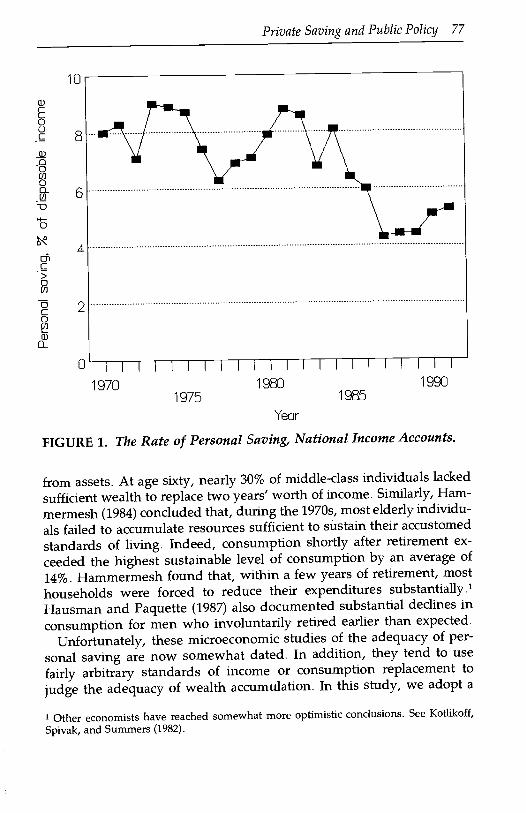
II. THE ADEQUACY OF PERSONAL SAVINGAccording to common wisdom, Americans consume too much and savetoo little. This impression is largely traceable to widely publicized statis-tics on aggregate personal saving. International comparisons reveal thatU.S. households save significantly less than their foreign counterparts.Between 1980 and 1989, Americans saved (net) 7.4% of disposable per-sonal income, compared with 11.4% for OECD Europe and 16.0% forJapan (OECD, 1989). Moreover, since the mid-1980s, the rate of house-hold saving in the United States has been well below its historical aver-age (see Figure 1).

Although these statistics raise legitimate concerns, they do not pro-vide definitive evidence of a problem. As measured, personal savingexcludes capital gains. Thus, households could in principle accumulatewealth at a rapid rate even when measured saving is low. Rates ofpersonal saving can also vary across both time and countries for reasonsunrelated to the adequacy of saving considered from the perspective ofindividual households. To understand this second point, consider thefollowing hypothetical example. Envision two countries, A and B, thatare identical in all respects, except that the elderly make up a largerfraction of the population in A than in B. Because households tend toaccumulate wealth prior to retirement and decumulate wealth there-after, one would expect to observe a higher rate of aggregate personalsaving in country B. Indeed, in an economy with no growth in eitherpopulation or productivity, dissaving by retirees could completely offsetsaving by workers: one could in principle observe no personal saving inthe aggregate, regardless of how well individual households preparedfor retirement. Thus, ultimately, one can only judge the adequacy ofpersonal saving by examining microeconomic data on the behavior ofindividual households.

Generally, the available evidence suggests that U.S. workers have pre-pared poorly for retirement. According to Diamond (1977), during the1960s roughly 40% of married couples and over 50% of unmarried indi-viduals reported that, after retirement, they received no money income

10

8

S

4

2


(I:)j I I I I I I I I I I I I I

1970 1980 19901975 1985

Year

FIGURE 1. The Rate of Personal Saving, National Income Accounts.

from assets. At age sixty, nearly 30% of middle-class individuals lackedsufficient wealth to replace two years' worth of income. Similarly, Ham-mermesh (1984) concluded that, during the 1970s, mostelderly individu-

als failed to accumulate resources sufficient to sustain their accustomedstandards of living. Indeed, consumption shortly after retirement ex-ceeded the highest sustainable level of consumption by an average of14%. Hammermesh found that, within a few years of retirement, mosthouseholds were forced to reduce their expenditures substantially.1

Hausman and Paquette (1987) also documented substantial declines inconsumption for men who involuntarily retired earlier than expected.

Unfortunately, these microeconomic studies of the adequacy of per-

sonal saving are now somewhat dated. In addition, they tend to usefairly arbitrary standards of income or consumption replacement tojudge the adequacy of wealth accumulation. In this study, we adopt a

1 Other economists have reached somewhat more optimistic conclusions. See Kotlikoff,

Spivak, and Summers (1982).


different strategy. Using an elaborate model of household decision mak-ing, we simulate asset accumulation profiles.2 We then compare thesesimulated profiles with actual profiles estimated from more recent house-hold survey data.

The simulation model uses a life cycle planning framework to establishthe criteria for household decision making. In this framework, a house-hold's standard of living at any point is taken to be a function of itsmaterial consumption per capita, and its overall well-being dependsupon both its present and future standards of living. Loosely speaking,the life cycle framework implies that a household should accumulatewealth sufficient to finance a standard of living during retirement that isconsistent with its standard of living prior to retirement.

The model takes as inputs certain descriptive data concerning a house-hold, including age, birth cohort, current earnings, pension coverage,education, marital status, and gender (if single). Based on these charac-teristics, the model imputes an earnings history, a family compositionhistory, and mortality probabilities. The earnings history is extrapolatedfrom cross-sectional age-earnings profiles and is adjusted to reflect theeconomy's baseline wage growth. Similarly, the family composition his-tory is constructed from estimates of the relationship between house-hold size and various household characteristics. Mortality probabilitiesare obtained from gender-specific actuarial tables. The model also incor-porates important macroeconomic factors, such as interest rates, in-flation, economic growth rates, aspects of the federal, state, and localincome tax systems, and social security statutes.

The model generates consumption and asset trajectories through aniterative procedure. The first step in this procedure determines thehousehold's asset accumulation plan for the first year of its economic life(taken to be age 26). The choice of a plan is based in part upon forecastsof its future economic prospects.3 Decisions taken in the initial yeardetermine the level of retirement assets that the household carries intothe following year. The second step of the procedure determines thehousehold's asset accumulation plan in its second year of economic life.Because the household may learn more about its economic prospectsbetween the first and the second years, its forecasts may change. Conse-quently, the household's second-year plan may deviate from the planthat it envisioned in the first year. For example, if during the secondyear, rates of interest rise unexpectedly, the household may decide to

2 Development of this model was sponsored by Merrill Lynch & Co., Inc. For a detaileddescription of the model, see Bernheim (1992b).

Forecasts of macroeconomic variables are calculated using simple econometric models.

70

60

50

40

20

10


AT hcome

Spend ig

0 ii I I I I I I I I I I II I II I I II I

27 33 39 45 51 57 63 69 75 81 87 93 9936 42 48 54 60 66 72 78 84 99 96 102

FIGURE 2. Simulated After-Tax Income and Consumption Trajectories.

take advantage of this development by saving more than it had plannedpreviously. Financial decisions taken in the second year establish thelevel of retirement assets carried over into the third year. This procedureis repeated, until the current year is reached. The household's assetaccumulation plan for the current year supplies the forecast for futureasset and consumption trajectories .'

It is important to understand that the model describes the accumula-tion of assets only for retirement. There are, of course, many reasons tosave. Households should prepare for the possibility of illness, layoff,disability, death, and other risks for which they are imperfectly insured.In addition, most households accumulate resources to pay for large ex-penses such as college tuition or the purchase of an automobile. In thecurrent study, no attempt is made to estimate the extent to which house-holds should save for these other reasons.

Figures 2 and 3 depict the output of an illustrative simulation run. This

It should be noted that, in each year, the model treats all forecasts of future prospects as ifthese prospects were known with certainty. Yet, in each decision year, additional informa-tion is acquired, and forecasts are revised. It would be preferable to employ a simulationmodel that would explicitly recognize uncertainty concerning future conditions and incorpo-rate this uncertainty into consumer decision making. However, this alternative approachposes considerable technical problems. The simplified approach adopted here probably hasthe effect of understanding the ideal level of asset accumulation, because, in the presence ofuncertainty, households would also have a precautionary motive for saving.


[I

O1O

C

Q)

r

350

3m

250

2c0

150

im

50

1IJ I I I I I I

27 33 39 45 51 57 63 69 75 81 87 93 99303642485460667278849096102ge

FIGURE 3. Simulated Wealth Trajectory.

particular simulation was constructed for a household with the follow-ing characteristics: age 27 (as of 1991), some college education, married,current earnings of $60,540, and the primary earner is covered by aprivate pension. Figure 2 displays, in constant 1991 dollars, this house-hold's trajectory of after-tax earned income (including pensions and so-cial security) and its consumption. Note that after-tax earnings risesteeply early in life. Earnings growth continues at a reduced level untilthe individual reaches age 55, at which point it begins to fall. Afterretirement, earned income consists of social security and private pensionbenefits. Because pensions are less than perfectly indexed for inflation,real benefits decline gradually over time.

As a direct consequence of its rapid earnings growth early in life, thehousehold saves nothing for retirement prior to age 30. In fact, during its20s, the household would prefer to borrow against future income inorder to consume more than its current after-tax income. However, the


model does not permit these households to obtain loans because theylack collateral. Between ages 30 and 80, the consumption trajectory isrelatively flat. This property reflects the household's preference for astable standard of living. However, during the 30s and 40s, consump-tion is somewhat elevated relative to the 60s and 70s. This pattern resultsfrom changes in household composition: between the ages of 30 and 50,the typical household incurs significant child-rearing costs. Consump-tion declines rapidly after age 80 until, at age 101, it matches after-taxretirement benefits. Falling survival probabilities drive this end-of-lifedecline. Because there is a relatively low probability of reaching age 90,the household would prefer to sacrifice the standard of living that itwould receive at age 90 (if it survived that long) in favor of a higherstandard of living earlier in life.

Figure 3 depicts the associated trajectory of retirement assets. Assetsare accumulated at an increasing rate early in life. They reach a peak atretirement and then steadily decline until they are exhausted at age 100.

Actual asset trajectories are estimated using the 1983 and 1986 wavesof the Survey of Consumer Finances (SCF). The Federal Reserve in con-junction with other federal agencies sponsored the SCF, and it is recog-nized as one of the best available sources for data on household balance

sheets.5We restrict attention to married couples for which the husband was

fully employed and between the ages of 25 and 64 in 1986. A total of1,314 households in the SCF sample satisfy these criteria. Our measureof accumulated net worth includes stocks and mutual funds, bonds,checking and savings accounts, IRA and Keogh accounts, moneymarketaccounts, certificates of deposit, profit sharing and thrift accounts, thedollar cash value of whole life insurance, and other financial assets, aswell as net equity in property (other than primary residences) and busi-ness assets, less credit card debt, consumer debt, and other debt.6 Thismeasure of net worth excludes all assets and liabilities associated withhomes and vehicles. This is appropriate because households appear tohave a strong aversion to paying living expenses during retirement byreducing home equity (see Venti and Wise, 1989); moreover, it seemslikely that few individuals save for retirement by accumulating wealth in

the form of vehicles.We divide the sample into two subgroups, based upon whether or not

See Avery and Elliehausen (1988) and Avery and Kennickell (1988) for a more completediscussion of the SCF.

6 Accumulated wealth for 1983 is expressed in 1986 dollars using the Consumer Price

Index.


the husband completed college. Our sample includes 474 husbands whocompleted college and 840 husbands who did not complete college.Education is of interest for two reasons. First, it may be related to differ-ences in behavior, either because education enhances an individual'sability to formulate coherent long-range plans, or because those whopursue more education do so precisely because they are more likely to beconcerned about the future. Second, education is highly correlated withincome. Adjusted for age, the median earnings of households in whichthe husband is college educated are roughly 57% higher than the medianearnings of households in which the husband is not college educated.Because IRA eligibility is subject to an ACT cap, differences in savingbehavior across income categories is of particular interest. Although itmight seem more natural to divide the sample by income in order toexamine these differences, that approach poses the practical difficultythat income varies with age. For example, a household with earnings of$50,000 at age 27 is probably much wealthier over the course of a lifetimethan a household with earnings of $55,000 at age 55. For this purpose,one can think of education as a proxy for permanent income.

As a first step in our analysis, we examine changes in wealth between1983 and 1986. In order to control for differences in resources acrosshouseholds, we focus our discussion on the ratio of the change in wealthto total wage income. We divide out sample into subgroups based uponage (25-29, 30-34, 34-39, 40-44, 45-49, 50-54, 55-59, 60-64). For eachof these subgroups, we calculate the median change-in-wealth-to-wagesratio (adjusting for sampling weights). The use of medians rather thanmeans is important, because the distribution of assets is highly skewed.Although mean wealth is quite high for many population subgroups,this fact tells us very little about the adequacy of saving for the typicalhousehold within these groups. Rather, it primarily reflects the extremebehavior of a few unrepresentative households. In contrast, medianwealth is not influenced by extreme outliers.

We then simulate asset accumulation trajectories for households thatare representative of each population subgroup. The household charac-teristics (wage income, years of education) chosen for these simulationsare based on within-subgroup population medians. Two simulations areconducted for each population subgroup: one assumes that the primaryearner is covered by a private pension, while the other assumes that theprimary earner is not covered by a private pension.

When one is comparing estimated and simulated trajectories, it isimportant to bear in mind that the simulations focus on preparation forretirement as the sole motive for saving. Unfortunately, when examin-ing the data, one cannot determine whether particular assets were accu-

0.25

0.2

0.15


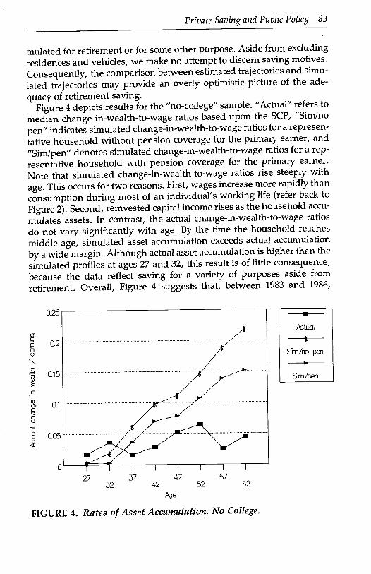
mulated for retirement or for some other purpose. Aside from excludingresidences and vehicles, we make no attempt to discern saving motives.Consequently, the comparison between estimated trajectories and simu-lated trajectories may provide an overly optimistic picture of the ade-quacy of retirement saving.

Figure 4 depicts results for the "no-college" sample. "Actual" refers to

median change-in-wealth-to-wage ratios based upon the SCF, "Sim/nopen" indicates simulated change-in-wealth-to-wage ratios for a represen-tative household without pension coverage for the primary earner, and"Simlpen" denotes simulated change-in-wealth-to-wage ratios for a rep-resentative household with pension coverage for the primary earner.Note that simulated change-in-wealth-to-wage ratios rise steeply withage. This occurs for two reasons. First, wages increase more rapidly thanconsumption during most of an individual's working life (refer back toFigure 2). Second, reinvested capital income rises as the household accu-mulates assets. In contrast, the actual change-in-wealth-to-wage ratiosdo not vary significantly with age. By the time the household reachesmiddle age, simulated asset accumulation exceeds actual accumulationby a wide margin. Although actual asset accumulation is higher than thesimulated profiles at ages 27 and 32, this result is of little consequence,because the data reflect saving for a variety of purposes aside fromretirement. Overall, Figure 4 suggests that, between 1983 and 1986,

I I I I I

27 37 47 5732 42

FIGURE 4. Rates of Asset Accumulation, No College.

52 62

Pctual

Sin/no pen

Sin/pen


0.5

1)]

0.4

0.3

0.2C0C

0.1

FIGURE 5. Rates of Asset Accumulation, College.

households without a college education saved far less than our simula-tion model predicts.

Figure 5 depicts results for the "college" sample. The contrast betweenFigures 4 and 5 is remarkable. In cases where the head of household hascompleted college, both simulated and actual change-in-wealth-to-wageratios rise steeply with age. Moreover, simulated asset accumulationtracks actual asset accumulation remarkably well. Taken at face value,Figure 5 suggests that college-educated households saved adequately forretirement between 1983 and 1986.

Low rates of asset accumulation do not necessarily imply that house-holds are inadequately prepared for retirement. In principle, a house-hold with high initial assets in 1983 (relative to the simulated trajectory)could save little between 1983 and 1986 and still remain above the simu-lated asset trajectory in 1986. Conversely, high rates of asset accumula-tion do not necessarily imply that households are adequately preparedfor retirement, because these households may have started out wellbelow the simulated trajectory. To evaluate the adequacy of retirementpreparation, one must therefore examine levels of wealth in addition tochanges in wealth.

Consequently, as a second step in our analysis, we examine levels ofwealth for 1986. We proceed exactly as in the first step, except that wefocus on wealth-to-wage ratios, rather than on change-in-wealth-to-wage

ktual$

Sin/no p&i

Sm/pen


27 37 4732 42

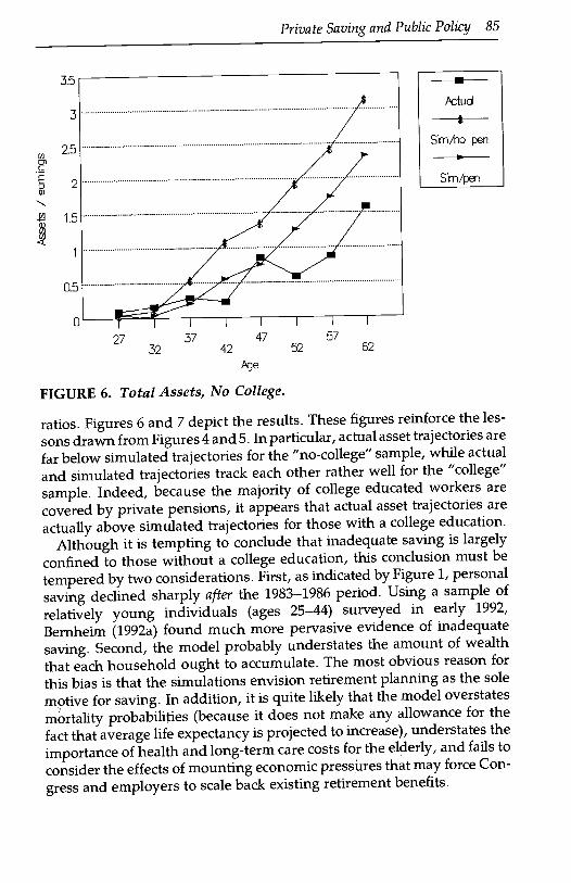
FIGURE 6. Total Assets, No College.

5752 62

-.ctuaI

8

Si-n/no pen

Sm/pen

ratios. Figures 6 and 7 depict the results. These figures reinforce the les-sons drawn from Figures4 and 5. In particular, actual asset trajectories arefar below simulated trajectories for the "no-college" sample, while actualand simulated trajectories track each other rather well for the "college"sample. Indeed, because the majority of college educated workers arecovered by private pensions, it appears that actual asset trajectories areactually above simulated trajectories for those with a college education.

Although it is tempting to conclude that inadequate saving is largelyconfined to those without a college education, this conclusion must betempered by two considerations. First, as indicated by Figure 1, personalsaving declined sharply after the 1983-1986 period. Using a sample ofrelatively young individuals (ages 25-44) surveyed in early 1992,Bemheim (1992a) found much more pervasive evidence of inadequatesaving. Second, the model probably understates the amount of wealththat each household ought to accumulate. The most obvious reason forthis bias is that the simulations envision retirement planning as the solemotive for saving. In addition, it is quite likely that the model overstatesmortality probabilities (because it does not make any allowance for thefact that average life expectancy is projected to increase), understates theimportance of health and long-term care costs for the elderly, and fails toconsider the effects of mounting economic pressures that may force Con-gress and employers to scale back existing retirement benefits.


ktua

Sin/no pen

Sm/pen

Bernheim (1992c) provides a more comprehensive discussion of the factors that couldproduce an inefficiently low level of saving within the standard life cycle framework.

27 37 4732 42

FIGURE 7. Total Assets, College.

Before one proceeds to the next section, it is important to discuss apotential criticism of this analysis. Some readers may be inclined toargue that our investigation sheds more light on the nature of tastes thanon the adequacy of saving for retirement (see, e.g., Lazear, 1992). Afterall, any measure of adequacy is subjective. If a household has chosen tosave relatively little, who are we to argue? Presumably, the householdhas its own best interests at heart.

We are not persuaded by this argument. Even in the context of thetraditional life cycle hypothesis, individuals may face incentives that leadto inefficiently low levels of saving. For example, as individuals savemore, they may lose the benefits from social insurance programs (Hub-bard, Skinner, and Zeldes, 1992), risk the loss of eligibility for collegescholarships (Feldstein, 1992), or reduce assistance from other membersof the extended family (Bernheim and Stark, 1988).7These considerationsmay be particularly important for lower-income individuals.

It is also possible that, for some households, the life cycle hypothesismay not adequately characterize saving behavior. For some economicdecisions, one can argue that, through trial and error, an individual

5752 62


eventually learns to behave in a way that is consistent with utility maxi-mization. This argument, however, is less persuasive in the context oflife cycle saving. Each individual accumulates resources for retirementonly once; there is no opportunity to learn from one's mistakes. More-over, the life cycle saving decision is extraordinarily complex, in that itrequires an individual to contemplate labor earnings, investment strate-gies, macroeconomic trends, and a vast assortment of risks, all over a

very long time frame. It would be surprising if the average individual, inisolation, with no practice and little or no training, would act as a per-fectly rational, farsighted utility maximizer. Manski (1993) discusses the

circumstances in which learning from others can take the place of per-sonal experience. Even with good role models and reference groups,however, it is difficult to imagine that households do not deviate fromtheir optimal life cycle consumption profiles.

In recent years, a number of economists have argued against the viewthat individuals act as if they maximize an intertemporal utility function,and have instead emphasized the importance of behavioral concepts

such as habit, mental accounting, and self-control (see, e.g., Shefrin andThaler, 1988). Behavioral theories allow for the possibility that individu-als may regret their bad habits and lack of foresight after the fact. Conse-

quently, the notion of inadequate saving has a clear normative meaningwithin the context of these theories.

The evidence offered in this section suggests that most householdswithout a college education do not behave in a manner consistent withoptimal life cycle planning. These households save little relative to their

simulated asset trajectories. Moreover, their estimated and simulatedtrajectories do not even exhibit the same qualitative patterns (refer onceagain to Figure 4).8 Given the behavioral differences between house-holds with and without college degrees, an important question arises: Is

it possible to design policies that effectively stimulate saving at all levels

of education and income?

III. PENSION POLICYIn recent years, asset accumulation in private pension plans has ac-counted for a substantial fraction of personal saving (see Bernheim and

It could be argued that low-income individuals save less relative to simulated savingbecause they discount the future more heavily. Although a higher discount factor wouldreduce saving, it would not alter the qualitative features of the asset trajectories (unlessdiscounting was high enough to prevent the accumulation of any significant assets for

retirement).


Shoven, 1988, and Bosworth, Burtless, and Sabelhaus, 1991). This obser-vation raises the possibility that policies affecting private pensions mayhave powerful effects on aggregate personal saving. Whether or notthese effects would actually materialize in practice depends upon themanner in which workers would respond to an expansion of privatepension coverage. Economic theory suggests that such an expansionwould simply crowd out other forms of personal saving. The simulationresults presented in section II illustrate this principle. However, previ-ous studies of personal saving generally fail to find evidence for thehypothesis that private pensions reduce other forms of personal saving(see, e.g., the review in Shefrin and Thaler, 1988, especially pp. 622-624). Depending upon whether one credits the theoretical analysis orthe empirical studies, one can reach dramatically different conclusionsabout the effect of pension policy on aggregate personal saving.

The analysis of section II raises an intriguing possibility: if the behav-ior of those with college education conforms to the predictions of the lifecycle hypothesis, while the behavior of those without a college educa-tion does not, then perhaps private pensions do displace personal sav-ing among the college educated, but do not displace personal savingamong the rest of the population. In this case, pension policy could bean effective tool for stimulating total personal saving, as long as it isprimarily used to provide incentives for expansion of coverage amonglower-income (less-educated) workers.

To investigate the effect of pensions on household saving, we estimateequations that explain the median value of the wealth-to-wage ratio(henceforth, WWRAT) as a function of the husband's age (AGE), totalhousehold earnings (EARN), and a dummy variable summarizing thehusband's private pension coverage (PENS).9 We employ a cubic func-tion of AGE to allow for flexible age-wealth trajectories. Because earn-ings may be related to the shape of the asset trajectory as well as to itsabsolute level, we also interact EARN with AGE. For similar reasons,PENS is interacted with AGE in most specifications.

For purposes of comparison with the previous literature, it is useful tobegin with results for the entire data sample (all households, irrespectiveof educational attainment). The following estimated equation is consis-tent with the view that pensions fail to displace other forms of personalsaving:

Because our object is to explain median wealth rather than mean wealth, we employquantile regression techniques (least absolute deviations), rather than more traditionalregression techniques (least-squared deviations).


WWRAT = 4.72 + 0.411 AGE - 0.115 (AGE)2/10 + 0.106 (AGE)3/103

(1.34) (0.098) (0.023) (0.017)

- 0.140 EARNI1O4 + 0.581 EARN x AGEI1O6 0.0004 PENS.(0.024) (0.045) (0.0379)

Note that the coefficient of the pension dummy is economically trivialand statistically insignificant.

The absence of a relationship between pension coverage and personalsaving is sometimes interpreted as providing evidence that standardeconomic models do not faithfully represent the typical household'sdecision-making process. Proponents of the standard model, however,argue that the absence of a pension effect is a statistical artifact. Pensioncoverage is not random. A worker who is concerned about retirement mayturn down job offers from employers who fail to provide attractive pen-sion benefits. Conversely, a worker who gives little thought to retire-ment may be unwilling to accept a job that provides pension coverage ifthis offer entails a reduction in current disposable income. If these hypo-

thetical facts are indeed descriptive of behavior, then those who areinclined to select jobs with pension coverage will tend to save more thanthose who are inclined to select jobs without pension coverage. For anyparticular individual, a private pension may displace other forms ofsaving; however, in the data, this pattern may be obscured by the factthat pension coverage is correlated with the inclination to save more. Inother words, a sample selection effect may offset the saving-displacement

effect.Unless we can determine whether the absence of a pension effect is a

behavioral phenomenon or a statistical artifact, we cannot predict theimpact of a change in pension policy on personal saving. We suggest amethod of distinguishing between these two hypotheses, based uponthe following argument. It is certainly possible that, by coincidence, asample selection effect exactly offsets the saving-displacement effect.However, the magnitude of the saving-displacement effect should varysystematically with age; specifically, the difference between the accumu-lated assets of those with pension coverage and those without pensioncoverage should increase with age. Although the sample selection effect

may also vary with age, it seems highly unlikely that these two effectswould exactly offset each other at every age.

We therefore estimate a new equation, in which an interaction terminvolving PENS and AGE is added to the list of explanatory variables.The estimated relationship is as follows:


WWRAT = 4.64 + 0.406 AGE - 0.114 (AGE)2/10 + 0.105 (AGE)3/103(1.47) (0.108) (0.025) (0.019)

- 0.137 EARN/b4 + 0.576 EARN x AGE/lU6 - 0.098 PENS(0.026) (0.049) (0.169)

+ 0.310 PENS x AGE/b2.(0.373)

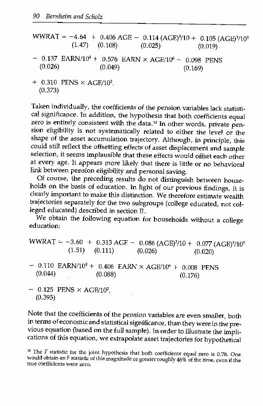
Taken individually, the coefficients of the pension variables lack statisti-cal significance. In addition, the hypothesis that both coefficients equalzero is entirely consistent with the data.10 In other words, private pen-sion eligibility is not systematically related to either the level or theshape of the asset accumulation trajectory. Although, in principle, thiscould stifi reflect the offsetting effects of asset displacement and sampleselection, it seems implausible that these effects would offset each otherat every age. It appears more likely that there is little or no behaviorallink between pension eligibility and personal saving.

Of course, the preceding results do not distinguish between house-holds on the basis of education. In light of our previous findings, it isclearly important to make this distinction. We therefore estimate wealthtrajectories separately for the two subgroups (college educated, not col-leged educated) described in section II.

We obtain the following equation for households without a collegeeducation:

WWRAT = 3.60 + 0.313 AGE - 0.086 (AGE)2/10 + 0.077 (AGE)3/b03(1.51) (0.111) (0.026) (0.020)

- 0.110 EARN/b4 + 0.406 EARN x AGE/b6 + 0.008 PENS(0.044) (0.088) (0.176)

- 0.125 PENS x AGE/b2.(0.395)

Note that the coefficients of the pension variables are even smaller, bothin terms of economic and statistical significance, than they were in the pre-vious equation (based on the full sample). In order to illustrate the impli-cations of this equation, we extrapolate asset trajectories for hypothetical10 The F statistic for the joint hypothesis that both coefficients equal zero is 0.78. Onewould obtain an F statistic of this magnitude or greater roughly 46% of the time, even if thetrue coefficients were zero.

1.8

1.6

0Li

0.8

0.6

0.4

0.2

27 37 47 575232 42

ge

FIGURE 8. Estimated Wealth Trajectories, No College.

households with pension coverage and households without pension cov-erage.11 Figure 8 exhibits these trajectories. Note that pension eligibilitybears little or no relationship to the path of the wealth-to-wage ratio.

In contrast, we estimate the following equation for households with acollege education:

WWRAT = 5.78 - 0.502 AGE + 0.126 (AGE)2/10 - 0.080 (AGE)3/103

(4.58) (0.329) (0.077) (0.058)

+ 0.062 EARN/104 - 0.021 EARN x AGE/b6 + 0.899 PENS - 2.83 PENS(0.048) (0.091) (0.563) (1.25)

x AGE/b2.

Note that the coefficients of the pension variables in this equation aremuch more significant, both economically and statistically. The data deci-sively reject the hypothesis that both of these coefficients equal zero.12

11 For the purpose of this calculation, the household's earnings are taken to be constant at$30,000. This figure is close to median age-adjusted earnings for households without acollege education.12 The F statistic for this hypothesis is 5.60, which is significant at the 99% level of confidence.


62

Pensb

No pensn


Note also that the signs of all the other coefficients in the equation forcollege-educated households are exactly the reverse of the signs of thesecoefficients in the equation for households without college education.Clearly, the behavior of these two groups differs markedly.

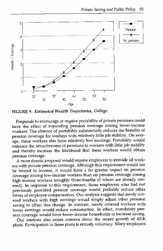
In order to illustrate the implications of the estimated equation forcollege-educated households, we extrapolate asset accumulation trajec-tories for hypothetical households with private pensions and withoutprivate pensions.13 Figure 9 depicts these trajectories. Note that thoseindividuals who are eligible for pensions accumulate resources at a signifi-cantly slower rate than those individuals withoutpensions. Remarkably,at age 62, the gap between the assets of these two groups is almost identi-cal in magnitude to the gap that emerges from our simulations (Figure 7).These patterns are strongly consistent with the view thatprivate pensionsdisplace other personal saving for college-educated households. It is un-likely that the observed relationship between pension coverage and sav-ing results from spurious factors, because such factors would presumablyalso have produced the same patterns for less-educated households.14These results suggest that previous studies may have failed to find asignificant saving displacement effect simply because they did not distin-guish between households on the basis of education.

The contrast between Figures 8 and 9 points to a clear and importantconclusion: private pensions displace personal wealth accumulation onlywhen the head of the household is college educated. This is consistentwith the findings of section lIon the adequacy ofpersonal saving. Indeed,our evidence tends to support a more general conclusion: college-educated households behave in the manner predicted by standard eco-nomic theories of saving, while households with less education do not.

It should be emphasized that past and current policies have been moresuccessful at stimulating the expansion of pension coverage amongcollege-educated workers than among those with less education. Analy-sis of the SCF data reveals that 75.2% of husbands with college degrees arecovered by private pensions, in comparison to 55.7% of husbands withoutcollege degrees. In other words, the current system is quite effective atproviding pensions to those who reduce other saving in response, but issubstantially less effective at providing coverage to those individuals forwhom pensions would represent incremental saving.

13 For the purpose of this calculation, the household's earnings are taken to be constant at$50,000. This figure is close to age-adjusted median earnings forhouseholds with a collegeeducation.

14 It is worth mentioning that there is some evidence of a small sample selection effect: thetrajectory for households with pensions starts out slightly above the trajectory for house-holds without pensions. However, this effect is not the dominant pattern in the data.

5

4

3

2

UI I I I I I I I

27 37 4732 42

qe


Pension

No pensbn

FIGURE 9. Estimated Wealth Trajectories, College.

Proposals to encourage or require portability of private pensions couldhave the effect of expanding pension coverage among lower-incomeworkers. The absence of portability substantially reduces the benefits ofpension coverage for workers with relatively little job stability. On aver-age, these workers also have relatively low earnings. Portability wouldenhance the attractiveness of pensions to workers with little job stabilityand thereby increase the likelihood that these workers would obtainpension coverage.

A more drastic proposal would require employers to provide all work-ers with private pension coverage. Although this requirement would notbe related to income, it would have a far greater impact on pensioncoverage among low-income workers than on pension coverage amonghigh-income workers (roughly three-fourths of whom are already cov-ered). In response to this requirement, those employers who had notpreviously provided pension coverage would probably reduce otherforms of employee compensation. Our analysis suggests that newly cov-ered workers with high earnings would simply adjust other personalsaving to offset this change. In contrast, newly covered workers withlower earnings would reduce consumption. In effect, mandatory pen-sion coverage would force lower-income households to increase saving.

Our analysis also raises concern about the recent growth of 401Kplans. Participation in these plans is entirely voluntary. Many employers

575252


have substituted 401K plans for more conventional plans in an effort toreduce operating expenses. We would not expect this trend to have asignificant impact on the total amount of saving done either by or onbehalf of high-income workers. However, the elimination of compulsorycontributions may significantly depress total saving by or on behalf oflower-income workers.

IV. TAX INCENTIVES FOR SAVINGThe most commonly discussed strategies for stimulating personal savingentail reductions in capital income taxation. Economic theory suggeststhat households will respond to a higher after-tax rate of return by in-creasing future consumption relative to current consumption. However,the increase in anticipated future net worth resulting from higher ratesof return may actually induce households to save less. Indeed, empiricalestimates of the interest elasticity of saving (which measures the sensitiv-ity of saving to the after-tax rate of return) vary widely (see, e.g., Boskin,1978; Summers, 1981; and Hall, 1988).

Current policies provide saving incentives primarily to lower-incomehouseholds. Eligibility for deductible IRAs, for example, is subject to anAGI cap. The existence of an AGI cap raises an important question:does the interest elasticity of saving vary systematically across incomeclasses?

Simulations based upon the model described in section II suggest thathigher-income households should be much more responsive than lower-income households to a change in the after-tax rate of return. Accordingto these simulations, a 35-year-old, high-school-educated couple withpension coverage and annual earnings of $30,000 in 1991 should havesaved roughly 1.5% of its earnings.15 A permanent, one percentage pointrise in the before-tax rate of return modestly increases this figure to1.6%. In contrast, a 35-year-old, college-educated couple with pensioncoverage and annual earnings of $50,000 in 1991 should have savedroughly 4.8% of its earnings. The same permanent, one percentage pointrise in the before-tax rate of return increases this figure by a much largeramount (both absolutely and proportionately), to 5.5%. Similar resultshold for couples without pensions. For the representative high-school-educated couple, saving would fall from 5.6% of earnings to 4.5% ofearnings in response to the higher rate of return; for the college-

15 In this calculation, the rate of saving is defined as saving above and beyond reinvest-ment of capital income, divided by after-tax wage income.


educated couple, it would fall less (both absolutely and proportionately),from 9.2% to 8.8%.16

The contrast between the simulated responses of college-educated in-dividuals and high-school-educated individuals becomes even morestriking when one factors in the statistics on pension coverage men-tioned at the end of section III. If one averages across those individualswith pensions and those individuals without pensions, the simulationsimply that saving by college-educated households would increase by10.2% in response to a permanent one percentage point increase in thebefore-tax rate of return, while the saving of households without collegedegrees would fall by 4.5%. Consequently, a policy that provides taxincentives for saving exclusively to lower-income households excludesthose households that are most likely to increase saving in response tothe policy; indeed, it is conceivable that such policies could actuallyreduce aggregate personal saving.

It is important to emphasize that this positive relationship betweenincome and the interest elasticity of saving results from a natural eco-nomic consideration, rather than from some peculiar feature of the simu-lation model. It is natural to assume that, when planning for the future,most households are concerned first and foremost with assuring them-selves of some minimum standard of living. As lifetime resources in-crease, households have more discretion to allocate resources over timein a way that increases consumption above and beyond this minimumstandard. Saving to provide for minimum consumption is, in effect,saving for a fixed target. It is well known that an individual who saves toachieve some target will reduce saving in response to an increase in therate of return (see, e.g., Bernheim and Shoven, 1988). In contrast, discre-tionary saving to finance consumption over and above the target re-sponds positively to an increase in the rate of return. For low-incomehouseholds, saving to achieve the minimum consumption target isprobably far more important than saving to fund incremental consump-tion. Thus, target saving dominates the simulated behavior of thesehouseholds, and produces a low or negative interest elasticity of saving.On the other hand, for high-income households, saving to fund incre-

16 These simulations imply that the interest elasticity of saving tends to be higher when thehousehold has private pension coverage. The explanation for thisphenomenon is straight-forward. An increase in the rate of return reduces the presentdiscounted value of futureincome; in that sense, it makes the household poorer, and reduces current consumption.(This effect was originally noted by Summers, 1981). Because pension income is receivedafter retirement, its present discounted value is more sensitive to the rate of return than isthe present discounted value of future (preretirement) earnings. Thus, those individualswith pensions are more likely than those individuals without pensions to reduce currentconsumption in response to an increase in the rate of return.


mental consumption is probably far more important than saving toachieve the minimum consumption target. Consequently, incrementalsaving dominates the simulated behavior of these households and pro-duces a high-interest elasticity of saving. In the appendix, we developthis argument mathematically and demonstrate for a simple model thatthe interest elasticity of saving rises with income.

Throughout this section, we have assumed that household behavioraccords with standard economic theories. The preceding sections callthis premise into question. However, this observation does not under-mine our conclusion. We have found that the behavior of college-educated (high-income) households does correspond to the predictionsof standard theories; consequently, for this group, it is likely that onewould observe a substantial interest elasticity of saving. On the otherhand, we have also found that the behavior of households without acollege education (those with lower income) does not conform to stan-dard economic theories. Although this finding reduces our faith in theapplicability of our simulation results, it does not reverse our conclu-sions concerning the interest elasticity of saving. The notion that house-holds will respond to a change in the after-tax rate of return is predicatedupon the assumption that households rationally anticipate and plan forfuture economic contingencies. To the extend that this assumptionproves incorrect, there is no particular reason to believe that low-incomehouseholds will respond to a change in the after-tax rate of return.

Most current proposals to provide tax incentives for saving are pat-terned after IRAs. IRAs were established as part of the 1974 EmployeeRetirement Income Security Act, to give workers who were not coveredby employer-provided pension plans added incentives to accumulateresources for retirement. In 1981, IRA eligibility was extended to alltaxpayers. Subsequently, the Tax Reform Act of 1986 curtailed the taxdeductibility of IRA contributions for high-income households.

Two prominent current policy initiatives would reverse the directionof the 1986 reforms and extend tax incentives for saving to households inhigher-income brackets. The Bush Administration's Family Saving Ac-counts (FSAs) would allow single individuals with incomes below$60,000 and married couples with incomes below $120,000 to make con-tributions of up to $2,500 per person (not including children) to qualifiedaccounts. The FSA proposal is an example of a "back-loaded" system:contributions are nondeductible, but accumulated funds are not taxedupon withdrawal. An alternative proposal, the Bentsen-Roth "super-IRA," would allow contributions of up to $2,000 per person (not includ-ing children) to either a traditional or a back-loaded IRA.

Unfortunately, there are sound conceptual reasons to doubt the effec-


tiveness of extending eligibility for IRA-style accounts to higher-incomehouseholds. First, contributions are capped. Under the current system,a single taxpayer, for example, can make no more than $2,000 in tax-deductible contributions. For any taxpayer who would have saved morethan $2,000 in the absence of IRAs, the availability of an IRA does notaffect the costs or the benefits that result from an additional dollar ofsaving and, therefore, provides no incentive on the margin for the tax-payer to increase saving. In such cases the IRA constitutes a "giveaway"of public funds, and its principal effect is to reduce federal tax receipts.In addition, the IRA may actually induce the taxpayer to spend more oncurrent consumption, because it increases his or her total after-tax re-sources. For both of these reasons, the IRA would contribute to a lowerrate of national saving. These concerns are of little significance for low-income households, because few of them would save more than $2,000in the absence of the program. It is far more likely that high-incomehouseholds would save more than the contribution limit Thus, a stan-dard IRA-style scheme may be a particularly ineffective method of pro-viding high-income households with tax incentives for saving.

Second, even if a taxpayer would not (in the absence of IRAs) havesaved more than the IRA contribution limit in a given year, he or shecould take full advantage of the IRA deduction either by drawing downpreviously accumulated assets or by borrowing. Indeed, the 1992 TaxGuide for College Teachers and Other College Personnel devotes a full page tothe issue, "What if You're Short of Cash to Fund Your IRA?" (pp. 229-230). The guide describes an IRS private letter ruling that allows house-holds to finance their IRAs by borrowing. Contributions funded eitherby shifting existing assets or by borrowing do not increase householdsaving. Instead, they depress national saving by reducing federal taxreceipts, and add to the federal budget deficit. Once again, high-incomehouseholds, who possess greater wealth, financial sophistication, andaccess to credit markets, are more likely than lower-income householdsto engage in borrowing or asset shifting and thereby defeat the purposeof the program.

Empirical evidence on the efficacy of IRAs is mixed. Gale and Scholz(1992) find little evidence that IRAs stimulated household saving be-tween 1983 and 1986. Venti and Wise (1986, 1987, 1990, 1991) andFeenberg and Skinner (1989) argue that most IRA contributions duringthis period represent net increases in household saving. Joines andManegold (1991) conclude that the effects of IRAs on household savingare unlikely to be as large as the estimates of Venti and Wise and may beas small as the estimates of Gale and Scholz.

An alternative proposal to promote household saving, based upon

98 Bernheim and Schulz

"Premium Saving Accounts" (PSA5), is described in Bernheim andScholz (1992). A PSA system would require each taxpayer to save in totalsome fixed amount (the "floor") before becoming eligible to make contri-butions to a tax-favored account. For each dollar saved in excess of thefloor, the taxpayer would be eligible to contribute one additional dollarto the tax-favored account, up to some limit ("the ceiling"). These floorsand ceilings would vary with AGI and certain types of capital income.As with IRAs, capital income accrued on balances held in PSA accountswould be exempt from taxation.17

The use of both floors and ceilings would create "windows" of pro-gram eligibility. Consider, for example, a husband and wife with a com-bined AGI of $80,000. They might face a floor of $8,000 and a ceiling of$12,000. Should they save less than $8,000 in the corresponding tax year,they would not be eligible to make any contributions to a tax-favoredaccount. If, on the other hand, they saved $9,500, they would be eligiblefor favorable tax treatment on $1,500. If they saved more than $12,000,then they would be eligible to make the maximum contribution of$4,000(the difference between $12,000 and $8,000).

The most important and distinctive feature of a PSA system is thatfloors and ceilings would vary with AGI. Eligibility windows could bepositioned to maximize, within each income class, the number of house-holds receiving tax breaks on the marginal dollar of saving. Thus,higher-income taxpayers would not be deprived of tax incentives forsaving; rather, they would simply be required to save large fractions oftheir incomes than lower-income taxpayers before becoming eligible forthe program. It would also be much more difficult for households to takeadvantage of tax-favored PSA accounts by shifting assets or by borrow-ing, because eligibility would be based upon total saving. An individualcannot increase total saving by shifting assets from one account to an-other or by borrowing in order to invest.18

To implement a PSA system, one needs to measure saving. Bernheimand Scholz (1992) propose the following measure:19

'' With this essential structure, a PSA system could be either front-loaded or back-loaded.Penalties could be established to lock funds into tax-favored accounts for relatively shortperiods of time (e.g., seven years), or until some age close to retirement (perhaps age 59k).Accounts could be established for specific purposes (e.g., retirement, purchase of a home,college education), or the accounts could be unrestricted.

18 The administrative feasibility of monitoring total saving for each taxpayer is discussed inBernheim and Scholz (1992).

19 Many economists would define saving as the change in the stock of wealth between twopoints in time. If one adopts this definition, then saving is very hard to measureonewould need to assess the market value of all assets every year. The definition used in thetext represents a compromise between economic logic and administrative feasibility.


Net purchases of assets (i.e., for assets on which investors receivecapital gains and losses, total purchases minus total sales),

plusThe January 1 to January 1 change in cash account balances (e.g.,bank accounts),

minusThe January 1 to January 1 change in total debt (e.g., mortgages andconsumer credit).

In effect, saving is defined as the incremental personal resources that anindividual diverts into investments in any given year, over and abovereinvested capital gains.20

If this definition of saving is employed, then it is also important toadjust each taxpayer's eligibility floors and ceilings upward by theamount of capital income other than capital gains. In the absence of suchan adjustment, the system would distort investors' choices among as-sets, causing them to tilt their portfolios toward assets that producecurrent income, rather than capital gains. See Bernheim and Scholz(1992) for a detailed discussion of this issue.

In the remainder of this section, we evaluate the effects of three dis-tinct strategies for stimulating household saving: an IRA-like programwith an ACT cap (henceforth referred to as the "standard IRA" system),an IRA-like program without an ACT cap (henceforth referred to as the"universal IRA" system), and a PSA system. We compare the cost-effectiveness of extending tax incentives for saving to higher-incometaxpayers through universal IRAs and PSAs.

Table 1 contains illustrative eligibility schedules for a PSA system. Weselected these particular schedules after examining the empirical distribu-

tion of saving. We restricted attention to a class of simple schedules andchose the schedules that provide maximum saving incentives.21

The schedules define eligibility windows for each level of ACI. Inorder to facilitate comparison with IRAs, we have adopted windowwidths of $2,000 per year for single households, $2,250 per year formarried couples with one earner, and $4,000 per year for married cou-ples with two earners. The lower end of the window (the floor) is deter-mined by a two-part calculation. First, compute the value of an algebraic

° Note that it is possible to compute this measure of saving without assessing the value ofunrealized capital assets because, by definition, unrealized gains are fully reinvested.

21 An eligibility schedule belongs to this class if the floor is set equal to zero up to somelevel of AGI, beyond which the floor rises linearly with AGI. We also studied morecomplex schedules but discovered that it was difficult to improve significantly upon thesimple schedule described in the text.


TABLE 1.Deductible Contribution Formula.

Deductible qualifiedcontribution floor

(added to capital income)

Deductible qualifiedcontribution ceiling

(added to floor)*If your income is

Married couplesLess than $34,000 0 $2,250 or $4,000Greater than $34,000 .167 x (Income - 34,000) $2,250 or $4,000

Single householdsLess than $42,000 0 $2,000Greater than $42,000 .34 X (Income - 42,000) $2,000

For the purpose of comparison with IRAs, married couples with one earner are allowed to contribute$2,250, and married couples with two earners can contribute $4,000. In the actual implementation ofthis proposal, we see no compelling reason to make this distinction.

expression involving ACT. We refer to this value as the "unadjustedfloor"it is identical for all taxpayers with the same level of ACT. Sec-ond, add capital income other than capital gains to obtain the "adjustedfloor" (or simply, "the floor"). Table 1 indicates, forexample, that a dual-earner married couple with an ACT of $30,000 and no capital incomewould have a floor of $0 and a ceiling of $4,000. In contrast, a couplewith an ACT of $120,000 and dividend and interest income of $2,000would have a floor of $16,362 (0.167 x $86,000 + $2,000) and a ceiling of$20,362. Figure 10 graphs the proposed eligibility schedule for marriedcouples. Note that because the typical U.S. household saves very little,the floor is zero for lower-income households.

The standard and universal IRA systems differ from the PSA proposalin that the IRA systems anchor the eligibilitywindow at $0 for all incomeclasses, and no adjustment is made for capital income. The standardsystem phases out deductible contributions for couples with incomesbetween $40,000 and $50,000 and for single taxpayers with incomes be-tween $25,000 and $35,000. The universal system allows all householdsto make deductible contributions.22

We will compare these plans on the basis of three criteria. The firstcriterion is a measure of effectiveness. Specifically, for each plan, weestimate the number of households that would receive a higher after-taxrate of return on the incremental dollar of investment. We refer to thesehouseholds as the TMPACT GROUP. Our second criteria is a measure ofwasteful subsidization. Specifically, for each plan, we estimate the num-

The IRA-like proposals we simulate are superior to actual IRA schemes, because, inpractice, IRA schemes are susceptible to tax arbitrage strategies involving borrowing andasset shifting, which our simulations do not capture.


hcome (Thousands)

FIGURE 10. PSA Eligibility Schedule, Married Couples (no capitalincome).

ber of households that would make the maximum eligible contributionto a tax-favored account while continuing to receive the unsubsidizedafter-tax rate of return on the incremental dollar of investment. We referto these households as the NO-IMPACT GROUP. Our third criterion isalso a measure of wasteful subsidization: we calculate the budgetary costof subsidizing the NO-IMPACT GROUP. We refer to this cost as theGIVEAWAY.

In evaluating these plans, it may be useful to consider other criteria,such as the ratio of the number of households in the IMPACT GROUPto the DOLLARS OF GIVEAWAY. A "bang-for-the-buck" ratio of thistype would provide some indication of the cost-effectiveness of eachproposal.

To calculate the size of the IMPACT GROUP, NO-IMPACT GROUP,and DOLLARS OF GIVEAWAY, we must predict the extent to whicheach household would participate in each plan. Our predictions arepredicated on three behavioral assumptions. First, we assume that nohousehold would make a contribution to any tax-favored account unless

200

I I

40 60 60 im 120


it would contribute to a universal IRA. Second, if a household wouldmake a contribution to a universal IRA, then that same household wouldalso, if eligible, contribute to either a standard IRA or a PSA. The justifi-cation for these first two assumptions is compelling: both proposals areidentical to the universal IRA system, except that eligibility is morerestricted.

Our third assumption concerns the magnitude of contributions. Foreach alternative proposal, we assume that an eligible household wouldmake the maximum allowable contribution when two conditions aresatisfied: the household would contribute to a universal IRA, and itstotal saving would exceed its eligibility ceiling. This third assumption ismore problematic than the others. Saving in a tax-favored account maybe an imperfect substitute for other forms of saving because, perhaps, ofrestrictions on early withdrawal. Thus, it is conceivable that some house-holds would contribute less than the maximum amount even whenthese conditions are satisfied. In practice, it would be very difficult toidentify these households with available data.

Obviously, our three assumptions are helpful only if we know whetheror not households are inclined to make contributions to universal IRAaccounts. During the period of universal IRA eligibility, this inclinationcan be inferred from actual behavior. Consequently, we base our calcula-tions upon a sample of households surveyed in 1983 and 1986 for whichdata on IRA participation are available.

More specifically, we use the 1983 and 1986 waves of the SCF. Keyvariables are constructed as follows. Income is defined as the average oftotal household income for 1983, 1984, and 1985. Our measure of savingcorresponds to the definition proposed earlier. To calculate the netchange in assets exclusive of capital gains or losses, we calculate (byasset category) the average constant contribution needed to generate thebalance in 1986, given the observed balance in 1983 and the average rateof return that prevailed during this period. Our asset categories includestocks and mutual funds, bonds, IRA and Keogh accounts, money mar-ket accounts, certificates of deposit, profit sharing and thrift accounts,the dollar cash value of whole life insurance, and other financial assets(for a more detailed discussion of the calculations, see Gale and Scholz,1992). Changes in cash account balances (saving and checking accounts)and total debt are measured directly.

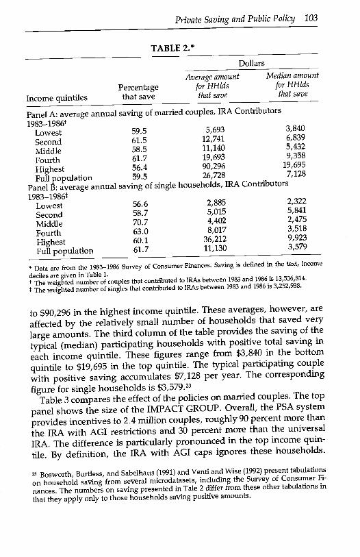
Table 2 provides background information on the saving propensitiesof households that contributed to IRA accounts. The top panel showsthat, on average across income groups, total saving was positive for only59.5 percent of participating couples. Among those households thatsaved, average saving ranged from $5,693 in the lowest income quintile

Income quintilesPercentagethat save

TABLE 2.*


Average amountfor HHldsthat save

Dollars

Median amountfor HHldsthat save

Data are from the 1983-1986 Survey of Consumer Finances. Saving is defined in the text, income

deciles are given in Table 1.The weighted number of couples that contributed toIRA5 between 1983 and 1986 is 13,536,814.

The weighted number of singles that contributed to IRA5 between 1983 and 1986 is 3,252,938.

to $90,296 in the highest income quintile. These averages, however, areaffected by the relatively small number of households that saved verylarge amounts. The third column of the table provides the saving of thetypical (median) participating households with positive total saving ineach income quintile. These figures range from $3,840 in the bottomquintile to $19,695 in the top quintile. The typical participating couplewith positive saving accumulates $7,128 per year. The correspondingfigure for single households is $3,579.23

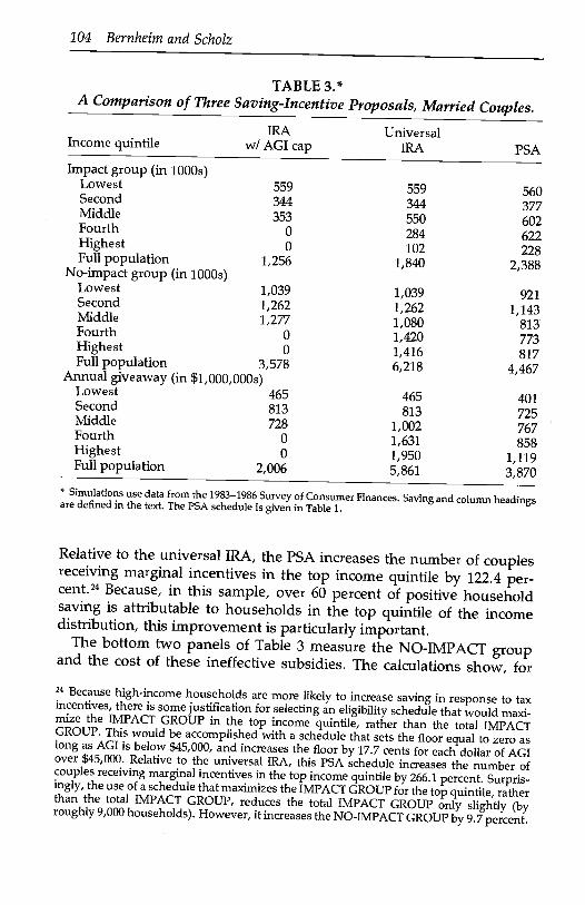
Table 3 compares the effect of the policies on married couples. The toppanel shows the size of the IMPACT GROUP. Overall, the PSA systemprovides incentives to 2.4 million couples, roughly 90 percent more thanthe IRA with AGI restrictions and 30 percent more than the universalIRA. The difference is particularly pronounced in the top income quin-tile. By definition, the IRA with AGI caps ignores these households.

Bosworth, Burtless, and Sabelhaus (1991) and Venti and Wise (1992) present tabulations

on household saving from several microdatasets, including the Survey of Consumer Fi-

nances. The numbers on saving presented in Tale 2 differ from these other tabulations in

that they apply only to those households saving positive amounts.

1983-1986LowestSecondMiddleFourthHighestFull population

56.658.770.763.060.161.7

2,8855,0154,4028,017

36,21211,130

2,3225,8412,4753,5189,9233,579

l9&3-l986LowestSecondMiddleFourthHighestFull population

Panel B: average annual

59.561.558.561.756.459.5

saving of

5,69312,74111,14019,69390,29626,728

single households, IRA

3,8406,8395,4329,358

19,6957,128

Contributors

Panel A: average annual saving of married couples, IRA Contributors


Income quintile

Simulations use data from the 1983-1986 Survey of Consumer Finances. Saving and column headingsare defined in the text. The PSA schedule is given in Table 1.

Relative to the universal IRA, the PSA increases the number of couplesreceiving marginal incentives in the top income quintile by 122.4 per-cent.24 Because, in this sample, over 60 percent of positive householdsaving is attributable to households in the top quintile of the incomedistribution, this improvement is particularly important.

The bottom two panels of Table 3 measure the NO-IMPACT groupand the cost of these ineffective subsidies. The calculations show, for

24 Because high-income households are more likely to increase saving in response to taxincentives, there is some justification for selecting an eligibility schedule that would maxi-mize the IMPACT GROUP in the top income quintile, rather than the total IMPACTGROUP. This would be accomplished with a schedule that sets the floor equal to zero aslong as AGI is below $45,000, and increases the floor by 17.7 cents for each dollar of AGIover $45,000. Relative to the universal IRA, this PSA schedule increases the number ofcouples receiving marginal incentives in the top income quintile by 266.1 percent. Surpris-ingly, the use of a schedule that maximizes the IMPACT GROUP for the top quintile, ratherthan the total IMPACT GROUP, reduces the total IMPACT GROUP only slightly (byroughly 9,000 households). However, it increases the NO-IMPACT GROUP by 9.7 percent.

Impact group (in l000s)Lowest 559 559 560Second 344 344 377Middle 353 550 602Fourth o 284 622Highest o 102 228Full population 1,256

No-impact group (in 1000s)1,840 2,388

Lowest 1,039 1,039 921Second 1,262 1,262 1,143Middle 1,277 1,080 813Fourth 0 1,420 773Highest o 1,416 817Full population 3,578Annual giveaway (in $1,000,000s)

6,218 4,467

Lowest 465 465 401Second 813 813 725Middle 728 1,002 767Fourth o 1,631 858Highest o 1,950 1,119Full population 2,006 5,861 3,870

TABLE 3*A Comparison of Three Saving-Incentive Proposals, Married Couples.

IRA UniversalwI AGI cap IRA PSA


TABLE 4*

A Comparison of Three Saving-Incentive Proposals, Single Taxpayers.

Simulations use data from the 1983-1986 Survey of Consumer Finances. Saving and column headings

are defined in the text. The PSA schedule is given in Table 1.

example, that the PSA system would reduce the number of householdsin the NO-IMPACT group by 1.75 million (28.2 percent) and would

reduce federal expenditures on ineffective subsidies by $2.0 billion (34.0percent), relative to the universal IRA. In terms of cost-effectiveness, thePSA system increases the ratio of the IMPACT GROUP to the GIVE-AWAY by 96.5 percent overall, and by 287.2 percent (i.e., by a factor of

almost four) in the top income quintile. The IRA with AGI caps alsoeffectively reduces ineffective subsidies and budgetary cost, but itachieves this reduction by excluding the very households that are most

likely to respond to tax incentives.Table 2 reveals that participating single households saved consider-

ably less than married households. Nevertheless, the gains from adopt-ing the PSA system would still be substantial for single households.Table 4 indicates that the size of the IMPACT group would increase by15.1 percent overall, and by 235.4 percent in the top-income quintile,relative to the universal IRA proposal. Moreover, both the size of the

Income quintileIRA

wI AGI capUniversal

IRA PSA

Impact group (in 1000s)Lowest 188 188 199

Second 105 105 150

Middle 136 173 173

Fourth 25 97 38

Highest 0 40 134

Full population 454 603 694

No-impact group (in l000s)Lowest 196 196 185

Second 280 280 236

Middle 312 275 275

Fourth 290 304 263

Highest 0 350 197

Full population 1,078 1,405 1,155

Annual giveaway (in $1,000,000s)Lowest 66 66 62

Second 141 141 117

Middle 168 158 158

Fourth 85 188 163

Highest 0 292 151

Full population 460 845 650


NO-IMPACT group and the GIVEAWAY would fall relative to the uni-versal IRA proposal. The result is a 49.7 percent increase in overall cost-effectiveness (the ratio of the IMPACT group to GIVEAWAY), and a551.3 percent increase in cost-effectiveness for the top quintile, relativeto the universal IRA proposal.

These comparisons of IRA and PSA proposals incompletely incorporatebehavioral responses. For example, households saving strictly less thanthe PSA eligibility floor might increase their saving in order to becomeeligible for PSAs. It is also possible that these proposals will differentiallyaffect saving for psychological reasons. Indeed, those who believe thatIRAs significantly stimulated private saving often suggest psychologicalexplanations, such as the following: (1) IRAs were aggressively marketedby financial institutions; (2) IRAs provided taxpayers with an effectiveway of earmarking funds for retirement, thereby facilitating the divisionof funds into distinct "mental accounts," some of which are psychologi-cally more difficult to invade; (3) the existence of a sizable early with-drawal penalty effectively locked saving into IRAs, thereby helpinghouseholds to impose self-discipline; and (4) the IRA eligibility limit pro-vided households with a saving "target." Empirical evidence suggeststhat the fourth effect was particularly important (many households con-tributed exactly $2,000, the widely publicized contribution limit, even incases where they were actually eligible to contribute more). The PSAsystem, like a universal IRA program, would preserve all these features.Indeed, the fourth effect would probably be strengthened with PSAs,because the proposal would provide many taxpayers with more ambi-tious targets.

V. CONCLUSIONSThe evidence presented in thispaper supports the view that many Ameri-cans, particularly those without a college education, save too little. Ouranalysis also indicates that it should be possible to increase total personalsaving among lower-income households by encouraging the formationand expansion of private pension plans. It is doubtful that favorable taxtreatment of capital income would stimulate significant additional savingby this group. Conversely, the expansion of private pensions wouldprobably have little effect on saving by higher-income households. How-ever, these households are more likely to increase saving significantly inresponse to favorable tax treatment of capital income. Currently, eligi-bility for IRAs is linked to an ACT cap, and pension coverage is morecommon among higher-income households than among low-income

households. The most effective system for promoting personal savingwould have precisely the opposite features.

Extending tax incentives for saving to higher-income households isproblematic. We have discussed three competing policy options: IRAs

with AGI caps, the universal IRA, and the PSA. Our analysis revealsthat the PSA system is a more cost-effective vehicle for providing saving

incentives to all households, particularly those in the top quintile of theincome distribution.

Pension policies and tax policies do not exhaust the full range ofstrategies for stimulating personal saving. One particular class of policies

not discussed here merits further attention. An accumulating body of

evidence, including that contained in sections II and III of this paper,suggests that the behavior of many households (particularly those withlower income) are not well described by traditional economic theories.Consequently, it may be possible to design more effective policies by

educating the population or by exploiting the psychology of saving. TheJapanese appear to have had considerable success with such a strategyduring the postwar period (see Horioka, 1988, and Bernheim, 1991). The

development of a framework for analyzing policies of this type is animportant research priority.

APPENDIX: HOUSEHOLD INCOME AND THEINTEREST ELASTICITY OF SAVING

Consider a two-period model, in which an individual maximizes

u(c11c2) = a_1[(ci - + p (c2 -

subject to

wpc1 +

1- ++r 1+r'

where c denotes consumption in the tth period of life (t = 1.2), r is theafter-tax rate of return, w is earnings in the first period, w is earnings inthe second period (the reader should construe this as pension income,

where < 1 is the replacement rate), m is minimum consumption, and a

is the (constant) elasticity of marginal utility with respect to consump-tion. Optimization requires

c2 - m = 'y(c1 - m)



where

y [/3(1 + r)]i.

Substituting this expression into the budget constraint and solving forfirst period saving (s = w - c1), we obtain

(1 + r)(w - m) + (w - m)s = (w - m) - l+r+yFrom this equation, we derive an expression for the interest elasticity ofsaving:

1rds T[1_((1+r)(1_a))j-sdr 1+r+y

where

+r)(wm)+(wj - m)y(wm)(pwm)

It is then apparent that

rydw L(1+r)1_a)1+r+y)jdw

It follows that the sign of d5/dw is the same as the sign of d/dw. But

d m(1+r+y)(1)dw [(y - p)w + m(1 -

which is positive if and only if i < 1. Thus, as long as income replace-ment during retirement is less than complete, the interest elasticity ofsaving rises with income.

REFERENCES

Avery, Robert B. and Gregory E. Elliehausen (1988), "1983 Survey of ConsumerFinances: Technical Manual and Codebook." Mimeo, Board of Governors ofthe Federal Reserve System, August.


and Arthur B. Kennickell (1988). "1986 Survey of Consumer Finances:Technical Manual and Codebook," Mimeo, Board of Governors of the FederalReserve System, November.

Bernheim, B. Douglas (1991). The Vanishing Nest Egg: Reflections on Saving inAmerica. Twentieth Century Fund, New York, NY.

(1992a), "Is the Baby Boom Generation Preparing Adequately for Retire-

ment? Summary Report." Mimeo, Princeton University, August.(1992b). "Is the Baby Boom Generation Preparing Adequately for Retire-

ment? Technical Report." Mimeo, Princeton University, August.(1992c). "A Discussion of Two Papers on Saving." Mimeo, prepared for

the Economics of Aging Conference in Caneel Bay, Princeton University,May.

and John Karl Scholz (1992). "Premium Saving Accounts: A Proposal toImprove Tax Incentives for Saving." Mimeo, Princeton University and theUniversity of WisconsinMadison, September.

,and John B. Shoven (1988). "Pension Funding and Saving." In Pensions inthe U.S. Economy, Zvi Bodie, John B. Shoven, and David A. Wise, eds., 85-111.Chicago: University of Chicago Press and NBER.

,and Oded Stark (1988). "Altruism Within the Family Reconsidered: DoNice Guys Finish Last?" American Economic Review 78, 1034-1045.

Bernstein, Allen (1991). 1992 Tax Guide for College Teachers and Other College Person-nel. Washington D.C.: Academic Information Services Inc.

Boskin, Michael (1978). "Taxation, Saving, and the Rate of Interest." Journal ofPolitical Economy April, 3-27.

Bosworth, Barry, Gary Burtless, and John Sabelhaus (1991). "The Decline inSaving: Evidence from Household Surveys." Brookings Papers on Economic Activ-

ity, 1, 183-241.Diamond, Peter A. (1977). "A Framework for Social Security Analysis." Journal of

Public Economics December, 275-298.Feenberg, Daniel R., and Jonathan Skinner (1989). "Sources of IRA Saving." In

Tax Policy and the Economy, Lawrence Summers, ed., 25-46. Cambridge, MA:The MIT Press.

Feldstein, Martin (1992). "College Scholarship Rules and Private Saving." NBERWorking Paper No. 4032, March.

Gale, William G., and John Karl Scholz (1992), "IRAs and Household Saving."Mimeo, UCLA and University of WisconsinMadison.

Hall, Robert (1988). "Intertemporal Substitution in Consumption," Journal ofPolitical Economy 96, 337-357.

Hamermesh, Daniel 5. (1984). "Consumption During Retirement: The MissingLink in the Life-Cycle." Review of Economics and Statistics February, 1-7.

Hausman, Jerry A., and Lynn Paquette (1987). "Involuntary Early Retirementand Consumption." In Work, Health and Income Among the Elderly. G. Burtless,ed., 151-175. Washington D.C.: Brookings Institution.

Horioka, Charles Y. (1988). "Why is Japan's Private Saving Rate So High?" InRecent Developments in Japanese Economics. R. Sato and T. Negishi, eds. Tokyo:Harcourt Brace Jovanovich Japan/Academic Press.

Hubbard, R. Glenn, Jonathan Skinner, and Stephen P. Zeldes (1992). "Pre-cautionary Saving and Social Insurance." Mimeo, Columbia University, April.

Joines, Douglas H., and James G. Manegold (1991). "IRA and Saving: EvidenceFrom a Panel of Taxpayers." Mimeo, U.S.C.


Kotlikoff, Laurence J., Avia Spivak, and Lawrence H. Summers (1982). "TheAdequacy of Saving." American Economic Review December, 1056-1069.

Lazear, Edward P. (1992). "Some Thoughts on Savings." Hoover InstitutionWorking Paper #E-92-17, June.

Manski, Charles F. (1993). "Dynamic Choice in a Social Setting: Learning Fromthe Experience of Others." Journal of Econometrics, 58, 121-136.

Organization for Economic Cooperation and Development (1989). OECD Eco-nomic Outlook, Historical Statistics, 1960-1 989, Organization for Economic Co-operation and Development: Paris, France.

Shefrin, Hersh M., and Richard H. Thaler (1988). "The Behavioral Life CycleHypothesis." Economic Inquiry 26, 609-643.

Summers, Lawrence (1981). "Capital Taxation in a Life Cycle Growth Model."American Economic Review September, 533-544.

(1985). "Issues in National Savings Policy." National Bureau of EconomicResearch Working Paper #1710, Cambridge, MA, September.

Venti, Steven F., and David A. Wise (1986). "Tax-Deferred Accounts, Con-strained Choice and Estimation of Individual Saving." Review of Economic Stud-ies LIII, 579-601.

and (1987). "IRAs and Saving." In The Effects of Taxation on CapitalAccumulation. Martin Feldstein, ed., 7-48. Chicago: University of ChicagoPress and NBER.

,and (1989). "Aging, Moving, and Housing Wealth." In The Eco-nomics of Aging. David A. Wise, ed. Chicago: University of Chicago Press andNBER.

and (1990). "Have IRAs Increased U.S. Saving?: Evidence fromConsumer Expenditure Surveys." Quarterly Journal of Economics 105, 661-698.

and (1991). "The Saving Effect of Tax-Deferred Retirement Ac-counts: Evidence from SIPP." In National Saving and Economic Performance, B.Douglas Bernheim and John B. Shoven, eds., 103-128. Chicago: University ofChicago Press and NBER.

and (1992). "Government Policy and Personal Retirement Sav-ing." Tax Policy and the Economy 6, 1-41.

Date post:	04-May-2018
Category:	Documents
Upload:	lekhanh
View:	217 times
Download:	0 times

Private Saving and Public Policy - National Bureau of ... · private saving is one component of ......

Documents