Private-Value Auctions, Resale, and CommonValue

Harrison Cheng and Guofu Tan�

Department of EconomicsUniversity of Southern California3620 South Vermont AvenueLos Angeles, CA 90089

May 12, 2009

Abstract

We establish the bid-equivalence between an independent private-value(IPV) �rst-price auction model with resale and a model of �rst-pricecommon-value auctions. The common value is de�ned by the transactionprice when trade takes place. When there is no trade, the common valueis de�ned through a monotonic extension of the resale price function. Weshow bid equivalence when (1) there are two bidders with a general resalemechanism; (2) there is one regular buyer and many speculators with amonopoly resale market; (3) there are two groups of identical bidders andthe winning bidder in the resale stage conducts a second-price auction tosell the object to the losing bidders. The buyer-speculators model of auc-tion with resale is bid-equivalent to the Wilson Drainage Tract commonvalue model. We assume that the resale market satis�es a weak e¢ ciencyproperty, which means that trade must be e¢ cient when the trade surplusis the highest possible under incomplete information. We show that whenthe weak e¢ ciency property fails, the bid equivalence result may fail.

�We want to thank Kalyan Chatterjee, Isa Hafalir, Vijay Krishna, Bernard Lebrun, Hao Li,Michael Schwarz, John Wooders, Lixin Ye and Charles Zheng for helpful comments. Financialassistance for visits to KIER, Kyoto University; ECARES, Belgium, and CAPOP, Penn Stateare gratefully acknowledged. Please contact Harrison Cheng at hacheng@usc.edu and GuofuTan at guofutan@usc.edu for comments and further suggestions.

1

1 Introduction

In this paper we study the way resale opportunities after the auction may a¤ectbidders�behavior in the auction. When resale is allowed after the auction, werefer to it as an auction with resale, and represent it by a two-stage game. Itis intuitively understood in the profession that resale is an important source ofcommon- value among the bidders. In the survey for their book, Kagel and Levin(2002, page 2) said that "There is a common-value element to most auctions.Bidders for an oil painting may purchase for their own pleasure, a private-valueelement, but they may also bid for investment and eventual resale, re�ectingthe common-value element". Comments re�ecting this conventional wisdomcan also be found, for example, in Ashenfelter and Genesove (1992), Chakra-vorti et al (1995), Cramton (1995), Hausman and Wittman (1993), McAfee andMcMillan (1987), McMillan (1994), Milgrom (1987), McMillan (1994), Rosen-thal and Wang (1996), Rothkopf and Harstad (1994).Earlier theoretical studies on the connection between resale and common

value were carried out in Haile (2000,2001,2003), Gupta and Lebrun (1999),and Lebrun (2007). The idea was exploited in Gupta and Lebrun (1999) andLebrun (2007) when the resale is a monopoly or monopsony market. Theo-retical implications of resale opportunities on auctions have been studied inBikhchandani and Huang (1989), Haile (2000, 2003) and Hafalir and Krishna(2008). Resale is sometimes assumed to have complete information to simplifythe analysis as in Milgrom (1987), Kamien et al. (1989), Gupta and Lebrun(1999), Gale et al. (2000) and Haile (2003).On the empirical side, Haile (2001) studied the empirical evidence of the

e¤ects of resale in the U.S. forest timber auctions. Haile, Hong, and Shum(2003) studied the U.S. forest lumber auctions and found the bidding data toconform to private-value auctions in some and common-value auctions in others.An explanation may be due to the presence or lack of resale. Hortascu and Kastl(2008) showed that bidding data for 3-month treasury bills are more like private-value auctions, but not so for 12-month treasure bills. The di¤erence may bedue to the relevance of resale in long term treasury bills. When an asset is heldin a longer period, there may be a need for resale, and this may a¤ect biddingbehavior.Restrictions on resale were often imposed by government agencies. In U.S.

forest timber auctions, third-party transfers were prohibited except in approvedcircumstances. Forest Service policy identifying these circumstances includedvague guidelines allowing transfers which "protect the interest of the UnitedStates" (U.S. Forest Service, 1976, 1981). However, resale in timber auctionscan take place through subcontracting as described by Haile (2001). In spectrumauctions held by many governments, there were often restrictions on resale. Forexample, in the British 3-G spectrum auctions1 of 2000, resale restrictions were

1The third-generation technology allows high speed data access to the internet. It washeld on Mar 6, 2000, and concluded on April 27, 2000, raising 22.5 billion pounds (2.5% ofthe GNP of UK). This revenue is seven times the original estimate. Five licenses A,B,C,D,E

2

imposed despite economists� recommendation to the contrary. It is not clearwhy the restrictions were imposed. It is possible that the government maylook bad when the bidders can turn around and resell for quick pro�ts after theauction2 . Bidders, however, �nd ways to circumvent such restrictions in the formof a change of ownership control. For example, a month after the British 3-Gauction, Orange, the winner of the license E, was acquired by France Telecom,yielding a pro�t of 2 billion pounds to Vodafone3 . The winner of the mostvaluable licence A is TIW (Telesystem International Wireless). In July 2000,Hutchison then sold 35% of its share in TIW to KPN and NTT DoCoMo withan estimated pro�t of 1.6 billion pounds4 .

Resale is sometimes conducted so that parties who did not or could notparticipate in the auction has a chance to acquire the object sold during theauction. This occurs for example in Bikhchandani and Huang (1989), wheregains to resale trade arise due to the presence of new buyers in the secondarymarket. We will focus on resale among bidders of the original auction. Thereare situations in which resale opportunities to a third party only a¤ect a bidder�svaluation of the object, and thus can be indirectly represented by a change invaluations. In this case, our model may allow third party participation. Howeverthird party participation may give rise to issues that are not explored here.By focusing on the resale among bidders, we study an interesting interaction

between resale in the second stage and bidding behavior in the �rst stage. Wewill in fact show that in private-value auctions with resale, the bidding data willbehave as if it is a common-value auction. This has been informally observed InGupta and Lebrun (1999), and Lebrun (2007) in cases when the resale marketis a simple monopoly or monopsony market. We will provide a theoreticalexamination for this intuition in more general resale environments. The mainidea of the paper is that it is the resale price, not the private valuation, whichdetermines the bidder behavior.We describe the phenomenon by the term "bid-equivalence". It means that

the bidding behavior of an independent private-value auction with resale is thesame as a pure common-value auction in which the common-value is de�ned bythe transaction price. The two auctions have the same equilibrium bid distrib-utions. The concept of bid-equivalence is slightly weaker than the observational

were o¤ered. Licence A was available for bidding by non-incumbent operators only. A moredetailed account is given in Klemperer (2004).

2Beyond the political and legal reasons, resale may facilitate collusions in the Englishauction as is shown in Garrat, Troger and Zheng (2007).

3Orange paid 4 billion pounds for the licence. In May of 2000, France telecom paid 6billion pounds more than the price Mannesmann had paid for it in October 1999 before theauction. Orange was the number three UK mobile group at the time. The reason for the resaleis due to a divestment agreement by Vodafone with the British government after acquiringMannesmann.

4TIW was a Canadian company based in Montreal and largely owned by Hutchison Wham-poa. The Hong Kong conglomerate) gained the upper hand when NTL Mobile, a joint ventureof the UK cable operator and France Telecom, withdrew from the bidding. The price of thelicence is 4.4 billion pounds. The pro�t is based on the implicit valuation of the license at 6billion in the transaction.

3

equivalence used in Green and La¤ont (1987). In observational equivalence,the payo¤s of the bidders and the revenue of the auctioneer are the same fortwo di¤erent auctions. In our bid-equivalence, the payo¤s of the bidders neednot be the same in auctions with resale and common-value auctions. La¤ontand Vuong (1996) showed that for any �xed number of bidders in a �rst-priceauction, any symmetric a¢ liated values model is observationally equivalent tosome symmetric a¢ liated private-values model. In a symmetric model, there isno incentive for resale. In our paper, we look at the asymmetric IPV auctionswith resale. We show that when bidders anticipate trading activities after theauction, the equilibrium bidding behavior is the same as in a common-valueauction. The gain from trade in our model is due to the asymmetric valuationsof the bidders in the beginning of the �rst stage. In Haile�s model, gain fromresale is due to di¤erent valuations at the resale stage due to arrival of newinformation. A discussion of the bid equivalence in Haile�s model is provided insection 6.For the case of two-bidder auctions with resale, we establish a very general

bid equivalence result. The framework is �exible enough to include a resaleprocess in which bidders make sequential o¤ers, or simultaneous o¤ers in theresale stage. The main assumption is a weak e¢ ciency property which saysthat trade should be e¢ cient (occur with probability one) when the trade sur-plus is the highest possible. It is easily satis�ed in most Bayesian bargainingequilibrium with sequential or simultaneous o¤ers. It rules out the no-tradeequilibrium in which there cannot be bid-equivalence. Our formulation of theweak e¢ ciency property is equivalent to the sure-trade property in Hafalir andKrishna (2008)5 .

The bid equivalence result holds more generally with many bidders. How-ever, the most general treatment cannot be o¤ered in this paper due to com-plexity. For the multiple bidders case, it seems likely that there may be morerestrictions on the resale mechanism for the bid equivalence result to hold. Inparticular the monopoly resale model may not work, as it violates the weake¢ ciency property when there are more than two buyers in the resale stage.A precise formulation of the resale mechanisms for the bid equivalence to holdis still in progress. With more than two bidders, a general existence result forthe auctions with resale is still lacking in the literature. The model of auctionswith resale with multiple asymmetric bidders is still not well-developed. Forthe bid equivalence result of this paper, we make two simplifying assumptions.First we assume that there are only two groups of bidders in the auction, andwithin each group, all bidders are identical. Secondly, in the resale stage, weassume that the winner of the auction sells the object by a second-price auctionto the losers of the auction. One advantage of using the second-price auctionresale mechanim is that it is e¢ cient so that after the resale, there is no need

5Hafalir and Krishna (2008) use it to show the bidding symmetry property of weak andstrong bidders in equilibrium. We use it to show the bid-equivalence result. In more generalmodels (such as a¢ liated signals or more than three bidders), bid equivalence may hold eventhough the symmetry property typically fails.

4

for further resales. Although this is not fully general, experimental or empiricalwork is likely to be conducted under similar simpli�cations in the beginning.Our result will provide a good foundation for further such studies. This is donein section 7.The bid-equivalence result may be somewhat surprising. One would expect

that resale only contributes a common-value "component" to the bidding behav-ior, and there is still a private-value component. Our result however says thatthe bidding behavior is the same as if it is a pure common-value model. Whathappens to private-value component? The answer is that bid-equivalence is trueonly in equilibrium, hence the private-value is still relevant out-of-equilibrium.Furthermore, the private-value is incorporated in the de�nition of the common-value, and is therefore indirectly a¤ecting the equilibrium bidding behavior. Inequilibrium, the payo¤s of bidders in the auction with resale is di¤erent from thepayo¤s in the common-value auction, even though the bidding behavior is thesame. Therefore, it is not correct to say that we have equilibrium equivalence.Auction with resale in general can be a very complicated game. The resale

game may involve potentially complicated sequences of o¤ers, rejections, andcounter-o¤ers. In-between the auction stage and the resale stage, there may bemany possible bid revelation rules that a¤ect the beliefs of the bargainers in theresale stage. We cannot deal with so many issues at the same time. For thebid revelation rule, we adopt the simplest framework of minimal information,i.e. that is there is no bid revelation in-between the two stages. Despite thelack of bid information, the bidders update their beliefs after winning or losingthe auction. Since bidders with di¤erent valuations bid di¤erently in the �rststage, the updated beliefs depend on the bid in the �rst stage. For this reason,there are heterogeneous beliefs in the resale stage. Furthermore, a bidder maybecome a seller or a buyer in the resale stage depending on the bidding behaviorin the �rst stage. This distinguishes the bargaining in the resale stage from thestandard bargaining game in the literature in which there is a �xed seller orbuyer, and the beliefs are homogeneous. The outcome of the bargaining ingeneral is di¤erent. For instance, the updating may improve the e¢ ciency ofthe bargaining compared to the standard homogenous model, as bargainers havebetter information.

One important implication of the bid equivalence result is that the equi-librium analysis of the two-stage auction with resale model is reduced to thesimpler equilibrium analysis of the one-stage common-value model. The revenueof the auction with resale is completely determined by the common-value func-tion, and the e¢ ciency of the auction with resale is determined by the tradingset as well as the common-value function. Applications of the bid equivalenceresult can be found in Cheng and Tan (2008) for the monopoly and monopsonycases and in Cheng and Tan (2009) for the general resale mechanism. Suchapplications enhance our understanding of the revenue impact of resale, andhow the revenue ranking of di¤erent auctions may be a¤ected by the resaleopportunities.The bid equivalence result also has important implications for the empirical

5

and experimental study of private vs. common value auctions such as Haile,Hong, and Shum (2003) and Hortascu and Kastl (2008). It implies that thedistinction between private and common value auctions is not purely a matterof which good is sold in the auctions. The existence of resale opportunities,and bidders�intention for resale are also important factors to consider. Someexperimental work has been done on the asymmetric auctions with resale model(see Georganas and Kagel (2009)). It is an interesting question to ask whetherbidders behave the same way in both models in practice or in experiments.Given the evidence that winner�s curse is observed in many experiments incommon-value auctions, it is interesting to see whether similar irrationality isobserved in the auctions with resale. There is strong empirical support for thebidding behavior in the Wilson drainage track model. It is also promising thatsuch support can be found in empirical studies of auctions with resale.

Section 2 presents the common value model. Section 3 describes the auctionwith resale model. Section 4 gives the bid equivalence result. Section 5 showsthat the buyer-speculators model of auction with resale is bid equivalent tothe Wilson tract model with one neighbor and many non-neighbors. Section 6discuss the di¤erence and similarities of our model and that of Haile. Section 7gives a bid equivalence result for the many bidders case when the seller conductsa second-price auction to sell the object to the losing bidders in the resale stage.

2 The Common-Value Model

There are M risk neutral bidders in an auction for a single object. Each bidderreceives a signal si 2 [0; s�i ] about the unknown common value of the object.Let Fi be the cumulative distribution of the signal si: Assume that Fi has acontinuous density function fi: The (expected) common value conditional onthe joint signal is denoted by w(s1; :::; sM ): All signals si are assumed to beindependent from each other. We refer to the function w as the common valuefunction. We will assume that the function w is continuously di¤erentiable,non-decreasing in each ti; w(0; 0) = 0; and w(t; t) is strictly increasing: Let bi(si)be a strictly increasing bidding strategy of bidder i; and ��1i be its inverse.The de�nition of �i can be extended beyond the bidding range if we let �(b) =

s�i when b is outside the range. LetZ zjZ0

jj 6=i denote the integration over all

signals except si; and the interval of integration for sj ; j 6= i is [0; zj ]: Let s�idenote the vector s = (s1; s2; ::; sM ) without the si component. Let dF�i(s�i) =Yj 6=idFj(sj): If a bidder i with signal si bids b; the expected pro�t in a �rst-price

auction is

�C =

Z �j(b)Z0

jj 6=i [w(si; s�i)� b]dF�i(s�i):

6

We say that b is an optimal bid if it maximizes �C : The bidding strategy pro�lebi(:); i = 1; 2; :::;M is called a Bayesian Nash equilibrium if each bi(si) is anoptimal bid.The signals can be normalized so that Fi is uniformly distributed over [0; 1]:

This normalization will be done in the case of two-bidder model and we let tidenote the normalized signal. Let bi(ti) be the strictly increasing equilibriumbidding strategy of bidder i in the �rst-price common-value auction, and �i(b) beits inverse. In the two-bidder model, we have the following �rst order conditionsatis�ed by the equilibrium bidding strategy

d ln�i(b)

db=

1

w(�1(b); �2(b))� bfor i = 1; 2: (1)

with the boundary conditions �i(0) = 0; ��11 (1) = ��12 (1). The ordinary di¤er-

ential equation system with the boundary conditions determine the equilibriumbidding strategy pro�le.

Although there are well-known equilibrium existence theorems for the �rst-price common-value auction, we will give a constructive proof of the equilibriumin the two-bidder model. This proof will be useful for us in the bid equivalenceresult. The proof makes use of the single crossing properties. A function h(t)satis�es the single crossing condition if h(t) � 0 when h(t0) � 0; and t > t0:The function h(t) satis�es the strict single crossing condition if h(t) > 0 whenh(t0) � 0; and t > t0: The function g(b; t) satis�es the strict single crossingdi¤erences condition if for all x0 > x; the function h(t) = g(x0; t)�g(x; t) satis�esthe strict single crossing condition. The function g(b; t) satis�es the smoothsingle crossing di¤erences condition if it satis�es the single crossing di¤erencescondition, and for all b; g1(b; t) = 0; � > 0; we must have g1(b; t + �) � 0; andg1(b; t� �) � 0:

Note that the equilibrium strategies in the following theorem depends onlyon the value of w on the diagonal f(t; t) : t 2 [0; 1]g: Our approach shows thatthe equilibrium is not a¤ected when w is modi�ed outside the diagonal.

Theorem 1 The pair of bidding strategies

bi(ti) =1

ti

Z ti

0

w(s; s)ds; ti > 0; bi(0) = 0

is an equilibrium in the �rst-price common-value auction with two bidders.

Proof. Since w(s; s) is a continuous function, bi is continuously di¤erentiable

in (0; 1]: By the L�Hopital rule, bi(ti)! 0 as ti ! 0: Hence bi is continuous on[0; 1]: Let �i = b

�1i be the inverse bidding function. Then �i is also continuously

di¤erentiable in (0; 1]: We have

tibi(ti) =

Z ti

0

w(s; s)ds (2)

7

Taking derivative of (2), we have

tib0i(ti) + bi(ti) = w(ti; ti):

Since �0i(b(ti)) =1

b0i(ti); we have

ti�i(bi(ti))

= w(ti; ti)� bi(ti)

or�i(b)

�0i(b)= w(�1(b); �2(b))� b for all b > 0;

and we know that the �rst-order conditions (1) are satis�ed by �i; i = 1; 2: Wewant to apply the Su¢ ciency Theorem (Theorem 4.2 of Milgrom (2004)). Let

g(b; t1) =

Z �2(b)

0

(w(t1; t2)� b)dt2

This function is continuously di¤erentiable in (b; t1): Let b0 > b: We have

g(b0; t1)� g(b; t1) = �(b0 � b)�2(b) +Z �2(b

0)

�2(b)

(w(t1; t2)� b0)dt2:

Since w is non-decreasing in t1; the single crossing di¤erences condition is sat-is�ed. The partial derivative of g with respect to b is

g1(b; t1) = (w(t1; �2(b))� b)�02(b)� �2(b):

Since w is monotonic in t1; the smooth single crossing di¤erences conditionis satis�ed. The Su¢ ciency Theorem then says that b1(t1) is an equilibriumstrategy of bidder one. The proof for bidder two is the same.

3 Auctions with Resale

Our model begins with an independent private-value (IPV) auction with resale.A pure common-value auction will be constructed from the IPV auction andthe resale process. Due to the complexity of the general multiple bidders case,we assume that there are two groups of bidders, group one and two with m;nmembers respectively. Each bidder has a private valuation whose cumulativedistribution is Fi(x) over [0; ai]: Bidders� private valuations are independentfrom other. In addition, in each group all bidders have the same Fi = F1 forgroup one and Fi = F2 for group two. We assume that each Fi is continuouslydi¤erentiable. Each bidder participates in a two stage game. In the �rst stage,a bidder makes a bid b in a �rst-price auction. We will only consider the casein which each bidder in the same group adopts the same strictly increasing

8

bidding strategy in the �rst stage (except the buyer-speculators in section 6).Let bk; k = 1; 2 be the strictly increasing bidding strategy of a group k bidder,and ��1k be the inverse bidding strategy. Since the maximum bid for a di¤erentgroup may be di¤erent, we de�ne �k(b) = ak; if b is outside the bidding range.The �rst-price auction with resale is a two-stage game. The bidders par-

ticipate in a standard sealed-bid �rst-price auction in the �rst stage. In thesecond stage, there is a resale game. At the end of the auction and before theresale stage, some information about the submitted bids may be available. Thedisclosed bid information in general changes the beliefs of the valuation of theother bidder. This may further change the outcome of the resale market. Weshall adopt the simplest formulation in which no bid information is disclosed6 .We call this the minimal information case. It should be noted that there is val-uation updating even if there is no disclosure of bid information, as informationabout the identity of the winner alone leads to updating of the beliefs.If a bidder i wins the auction, she may sell it to the losing bidders in the

resale stage. If she loses the auction, she may buy it from the winning bidder.Her belief about group k bidders� valuations after winning the auction is Fkconditional on [0; �k(b)]: If she loses the auction, the belief is Fk conditional on[�k(b); ak]: This belief system in the resale stage is common knowledge.Since bidder i with di¤erent valuations bid di¤erently in the �rst stage,

they have di¤erent updated beliefs in the resale game. We refer to this asheterogeneous belief as a contrast to the standard multi-lateral trade modelin which a trader�s belief is independent of his valuation. We refer to this ashomogeneous beliefs. The equilibrium behavior in the second stage resale gameis therefore di¤erent from the standard bargaining model with homogeneousbeliefs. Furthermore, each trader in the resale trade game may be a seller ora buyer depending on whether he wins or loses the auction in the �rst stage.This endogenous determination of the seller-buyer role is also absent from thestandard bargaining model with homogeneous beliefs.A trader�s strategy in the resale game is therefore a¤ected by her bid bi in

the �rst-stage auction, and whether she wins or loses the �rst-stage auction. Sheis not a¤ected by bj of the other bidders as they are not observable. We do notneed to explicitly specify the resale game. Let �wk (:; bk(:)) be the strategy in thesecond stage when the bidder is in group k; and wins the auction. If the bidderloses the auction, and another bidder of the same group wins the auction, weassume that there is no resale activity for the bidder, and a strategy need notbe speci�ed. Let �lk(:; bk(:)) be the bidder�s buying strategy in the second stagewhen the a member from another group wins. Each bidder has such a pair ofstrategies in the resale game. In equilibrium, we require that each �wi (xi; bi(xi))is an optimal response to �lj(:; bj(:)); j =2 i; and each �li(xi; bi(xi)) is an optimal

6Although the equivalence result may be established in a broader context with disclosureof di¤erent bid information, it is su¢ cient to restrict ourselves to the resale market with nodisclosure of bid information in this paper. Lebrun (2007) has shown that an equilibrium withbid disclosure is observationally equivalent to an equilibrium with no bid disclosure. Thereforethe bid equivalence can be extended to the bid disclosure case. Haile (2001,2003) allowed biddisclosure in his model and this is discussed in section 6 below.

9

response to �cj(:; bj(:)); j =2 i; c = w for exactly one j from a di¤erent group:We call this a Bayesian Nash equilibrium of the resale game. According to therevelation principle, there is a direct trade mechanismMk; k = 1; 2 in the resalestage in which truth-telling is incentive compatible and individually rationalwith the same equilibrium outcome. The mechanism Mk refers to the casewhen a group k members wins. We have suppressed the dependence on thebidding strategies bk; k = 1; 2: We also need to consider the case when a bidderi deviates to the bid bi; and let the resulting direct mechanism be denoted byMk(bi):In the direct trade mechanism, given the reported valuations, x = (xi)

m+ni=1 ;

when bidder i in group one wins the auction, let qw(x; bi) be the probabilityof trade, and pw(x; bi) be the price of the transaction. When she loses theauction, let ql(x; bi); pl(x; bi) be the probability of trade and transsaction pricerespectively. If she wins the auction, let R1(b) be the revenue from selling theobject in the resale stage (when there is no resale, the revenue is assumed to beher own valuation). We have the expected revenue

R1(b) = E [(pw(xi; x�i)q

w(xi; x�i) + (1� qw(xi; x�i))xijxi; b] :

If she loses the auction, the (net) pro�t from buying the object in the resalegame is

R2(b) = E�(xi � pl(xi; x�i))ql(xi; x�i)jxi; b

�:

The net pro�t from bidding b is given by

�R = R1(b) +R2(b)� bFm�11 (�1(b))Fn2 (�2(b)): (3)

Similarly, we can de�ne R1(b); R2(b); and the pro�t function of a group twobidder j bidding b given by

�R = R1(b) +R2(b)� bFm1 (�1(b))Fn�12 (�2(b)):

The bid b is optimal if it maximizes �R: The bidding strategy pro�le b1(:); b2(:)in the �rst-stage auction is a perfect Bayesian Nash equilibrium if each bk(z) isan optimal bid for a bidder in group k = 1; 2 with valuation z: In this de�nition,the equilibrium property in the �rst stage relies on the mechanism Mk(bi) ofthe second stage; and at the same time, the equilibrium in the resale game alsorelies on the belief system genereted by the bidding strategies bk; k = 1; 2:

For the rest of the section, we consider the two-bidder case. We �nd ituseful to adopt a signal representation of the IPV model. This representation(called a distributional approach) is �rst proposed in Milgrom and Weber (1985)and discussed extensively in Milgrom (2004). This will allow us to apply themodel to the case of discrete distributions, and make good use of the propertyof symmetric bid distributions in the two-bidder model.In this representation, a bidder is described by an increasing valuation func-

tion vi(ti) : [0; 1] ! [0; ai]; with the interpretation that vi(ti) is the private

10

valuation of bidder i when he or she receives the private signal ti: We can nor-malize the signals so that both signals are uniformly distributed over [0; 1]. Thetwo signals are assumed to be independent: The word �private� refers to theimportant property that bidder i�s valuation is not a¤ected by the signal tj ofthe other bidder, while in the common-value model, this is not the case. Thefunction vi(ti) induces a distribution on [0; ai]; whose cumulative probabilitydistribution is given by Fi(xi) = v

�1i (xi): If v1(t) � v2(t) for all t; we say that

bidder one is the weak bidder, bidder two is the strong bidder, and the pair is aweak-strong pair of bidders7 . This is equivalent to saying that F1 is �rst-orderstochastically dominated by F2.Let qw(x1; x2; b1); pw(x1; x2; b1) be the allocation and pricing system when

bidder one wins, and ql(x1; x2); pl(x1; x2) when bidder one loses. We shallassume that the resale game satis�es the following weak e¢ ciency propertyqw(x1; �2(b1); b1) = 1 if either bidder one with valuation x1 wins the auctionand x1 � �2(b1); or bidder one loses the auction and x1 � �2(b1): Note thatthe pair (x1; �2(b1)) has the highest trade surplus. E¢ ciency for the pair meansthat transaction must takes place for this pair. It is a weak e¢ ciency propertyfor the resale mechanism because it only requires e¢ ciency for the pair with thehighest trade surplus8 .In equilibrium b1 = b1(x1), we can just write qw(x1; x2); pw(x1; x2; ) for

qw(x1; x2; b1); pw(x1; x2; b1) respectively. Furthermore, winning and losing cases

are mutually exclusive, and the underlying mechanism is clearly understood.Therefore, we shall skip the superscript and just write q(x1; x2); p(x1; x2; ):Let Q be the set of (t1; t2) such that q(x1(t1); x2(t2)) = 1 and assume thatp(v1(t1); v2(t2)) is nondecreasing in each variable, continuously di¤erentiable onQ; and p(v1(t); v2(t)) is strictly increasing in t: The set Q determines whetherthere is resale, and who gets the good at the end. Therefore it is important forthe study of e¢ ciency properties of the auctions with resale.

Let b� be the maximum bid of the bidders. By Proposition 3 (section 5.1)of Hafalir and Krishna (2008), the following �rst-order condition and symmetryproperty hold for the equilibrium of auction of resale.

Proposition 2 If the inverse equilibrium bidding functions �i; i = 1; 2 are dif-ferentiable in (0; b�]; then the following �rst-order conditions are satis�ed

d lnFi(�i(b)))

db=

1

p(�1(b); �2(b))� b; i = 1; 2; b 2 (0; b�]: (4)

and we have F1(�1(b)) = F2(�2(b)) for all b 2 [0; b�]:7Here we only require that F1 is dominated by F2 in the sense of the �rst order stochastic

dominance. Note that this concept is weaker than that of Maskin and Riley (2000), in whichconditional stochastic dominance is imposed.

8 It can be shown that in a standard bilateral trade with incomplete information, an incen-tive e¢ cient mechanism automatically satis�es the weak e¢ cient property. The bargainingmodel here is not a standard one due to heterogeneous beliefs. However, we believe that thesame result should hold in this case as well.

11

In most interesting bilateral trade models, such as k�double auctions orsequential bargaining models, it is often the case that trade takes place withprobability 0 or 1: For the standard bilateral trade model, Myerson and Sat-terthwaite (1983) and Satterthwaite and Williams (1989) have shown that tradeoccurs with probability 1 or 0 when they are incentive e¢ cient. In this case, Q isthe set of pairs for which trade occurs for sure, and outside Q there is no trade.The description of the resale process includes most of the well-known equilibriummodels of bilateral bargaining between the seller and the buyer. The followingexamples illustrate some of the most often used models of bilateral trade.

Example 3 Monopoly or Monopsony Resale

There is a weak bidder (one) and a strong bidder (two). Assume that thewinner of the auction is the monopolist seller in the resale game. This is themonopoly resale model (with commiment). The monopolist makes a take-it-or-leave-it o¤er, and the transaction price is the optimal monopoly price. Bidderone with signal t1 has the valuation v1(t1) and bids b in the �rst stage. When shewins the auction, she believes that bidder two�s valuation is F2 over [0; �2(b)]: If�2(b) � v1(t1); bidder one makes an optimal o¤er to bidder two. Assume thatthere is a uniquely determined optimal o¤er (equilibrium) price p(t1; b): Thentrade takes plance if and only if v2(t2) � p(t1; b). If she loses the auction, and�2(b) � v1(t1); then bidder two is the monopolist, and makes o¤ers to bidderone. Let p(t2; b) be the optimal monopoly o¤er of bidder two, then trades takesplace if and only if v1(t1) � p(t2; b): In equilibrium, only bidder one makeso¤ers, and we have Q = f(t1; t2) : t1 � t2; v2(t2) � p(t1; b1(t1))g: Hence tradeoccurs if and only if (t1; t2) 2 Q; and the trading price is the optimal o¤erprice p(t1; b1(t1)). Note that the weak e¢ ciency property is satis�ed becasuean optimal monopolist price does not exceed the highest valuation buyer, sothat trade occurs with probability 1 when the buyer has the highest valuation�2(b1(t1)):Similarly, in a monopsony resale mechanism with a take-it-or-leave-it o¤er

by the buyer, the buyer chooses an optimal monopsony price higher than thelowest possible valuation of the seller. The o¤er is accepted when the sellerhas the lowest valuation, hence the weak e¢ ciency property also holds, and thetransaction price is the optimal monopsony price. In equilibrium only biddertwo makes o¤ers.Another variation is to designate one of the bidder, say bidder one, as the

o¤er-maker. When it is not a weak-strong pair, bidder one may become aseller or a buyer depending on the realized signals. Thus it is a mixture of themonopoly and the monopsony market. The choice of the o¤er-maker or themarket type a¤ects the bargaining power of the bidders and the outcome ofthe resale. In the case of the monopoly market mechanism, the choice of theo¤er-maker is not �xed in the beginning, and is contingent on the outcome ofthe auction.

12

Example 4 Endogeneous Determination of Buyer-Seller Role

To illustrate the endogenous nature of the seller or buyer role in the resale,let the bidders�valuation distributions be given by F1(x) = x;

F2(y) = 2y2 when y 2 [0; 0:5]= 4y � 2y2 � 1 when y 2 [0:5; 1]

The resale is a monopoly. In equilibrium, if x < 0:5; bidder one bids b1(x) andwins the auction, he is the seller. The optimal monopoly price is

p =2x+

p4x2 + 6x

6:

Trade occurs if y � p or

t2 � 2(2x+

p4x2 + 6x

6)2

There is no resale, if he loses the auction. If x > 0:5; and bidder one wins theauction, there is no resale. If he loses the auction, he is a buyer. the optimalo¤er by buyer two with valuation y = F�12 (t) is

p =1

2(t+ 1)� 1

4

p2� 2t:

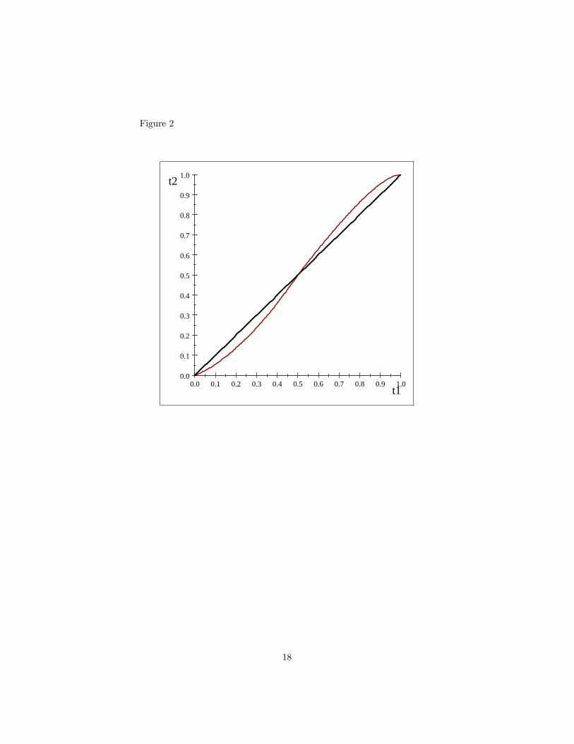
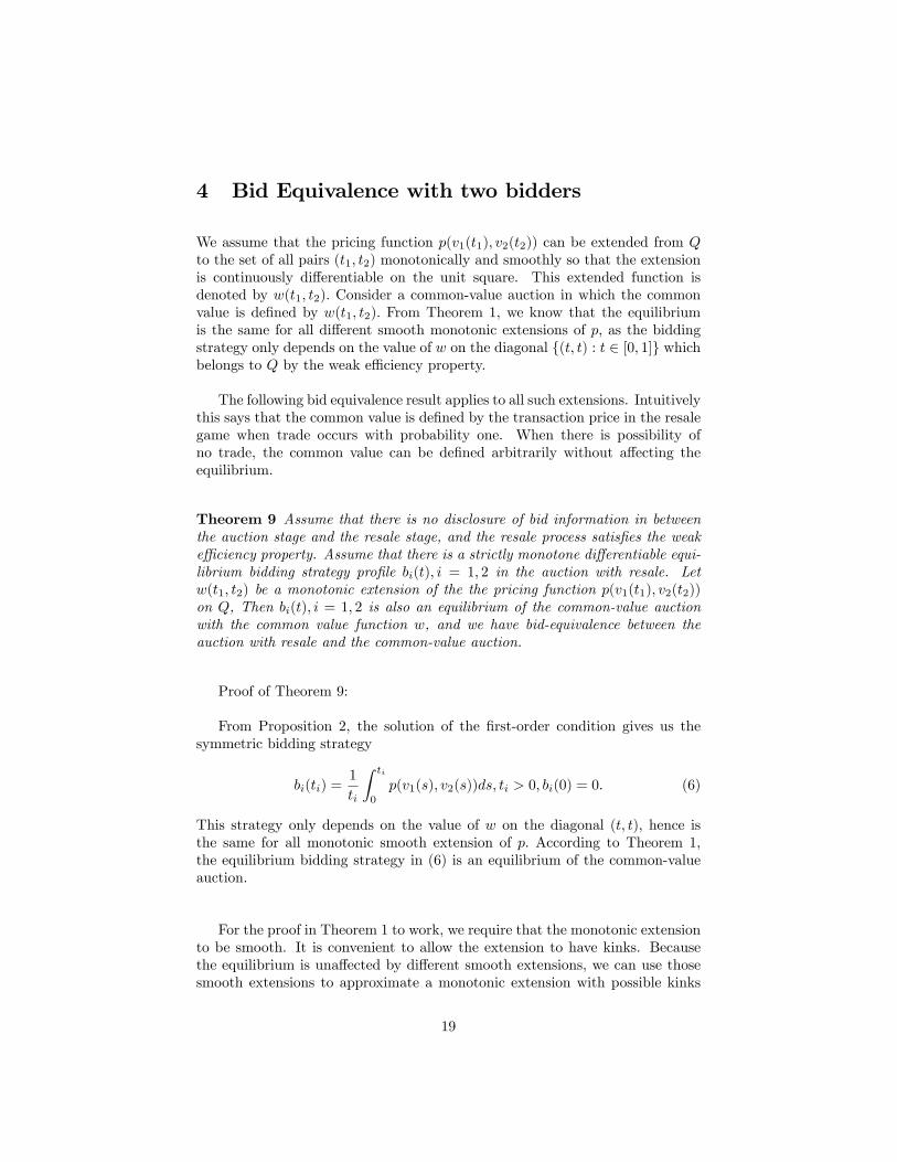
There is trade if x � p: The graph is plotted in Figure 2. The trading set Q isthe union of the two areas bounded by the straight line and the red curve.

The folliowing illustrates a monopoly resale model when the monopolistcannot credibly commit to her o¤ers in the �rst period, and engage in sequentialo¤ers to sell the good with a delay cost.

Example 5 Resale Markets with Sequential O¤ers

Consider a bargaining model with two rounds of o¤ers by the seller. As-sume that signals are independent, and we have a weak-strong pair. The sellerwith the signal t1 and the valuation v1(t1) makes an o¤er P1 in the �rst pe-riod. This o¤er is either accepted or rejected, with the threshold of acceptancerepresented by Z; i:e: a buyer accepts the �rst o¤er if and only if his or hervaluation is above Z: If the �rst o¤er is accepted, the game ends. If it isnot accepted, the seller makes a second o¤er P2 which is a take-it-or-leave-it o¤er. Let P1(t1); P2(t1); Z(t1) denote the equilibrium �rst-period, second-period prices and threshold level in this bargaining problem. Given the reported(v1(t1); v2(t2)); bidder one makes the �rst o¤er if she wins the auction: There isno trade if v2(t2) < P2(t1): Trade occurs (with probability one) with the trans-action price p(v1(t1); v2(t2)) = P1(t1) if v2(t2) � Z(t1); and the transactionprice p(v1(t1); v2(t2)) = �P2(t2) if P2(t1) � v2(t2) < Z(t1): The set Q is

Q = f(t1; t2) : t1 � t2; v2(t2) � Z(t1) or P2(t1) � v2(t2) < Z(t1)g

13

There is no trade when the pair is not in Q: The weak e¢ ciency property issatis�ed because we must have Z(t1) < v2(t2); and we have p(v1(t1); v2(t2)) =P1(t1): The weak e¢ ciency property holds in a monopoly resale mechanism withmany rounds of o¤ers from the seller, if the equilibrium �rst o¤er is lower thanthe highest valuation of the buyer. This is true if the monopolist has a strictlypositive payo¤ in the equilibrium.

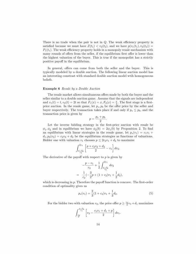
In general, o¤ers can come from both the seller and the buyer. This istypically modeled by a double auction. The following linear auction model hasan interesting constrast with standard double auction model wtih homogeneousbeliefs.

Example 6 Resale by a Double Auction

The resale market allows simultaneous o¤ers made by both the buyer and theseller similar to a double auction game. Assume that the signals are independentand v1(t) = t; v2(t) = 2t so that F1(x) = x; F2(x) = x

2 : The �rst stage is a �rst-price auction. In the resale game, let ps; pb be the o¤er price by the seller andbuyer respectively. The transaction takes place if and only if ps � pb; and thetransaction price is given by

p =ps + pb2

:

Let the inverse bidding strategy in the �rst-price auction with resale be�1; �2 and in equilibrium we have �2(b) = 2�1(b) by Proposition 2: To �ndan equilibrium with linear strategies in the resale game, let ps(v1) = c1v1 +d1; pb(v2) = c2v2 + d2 be the equilibrium strategies as functions of valuations:Bidder one with valuation v1 chooses p � 2c2v1 + d2 to maximizeZ 2v1

p�d2c2

�p+ c2v2 + d2

2� v1

�dv2:

The derivative of the payo¤ with respect to p is given by

�p� v1c2

+1

2

Z 2v1

p�d2c2

dv2

=1

c2(�32p+ (1 + c2)v1 +

1

2d2);

which is decreasing in p: Therefore the payo¤ function is concave. The �rst-ordercondition of optimality gives us

ps(v1) =2

3(1 + c2)v1 +

1

3d2: (5)

For the bidder two with valuation v2; the price o¤er p � v22 c1+d1 maximizesZ p�d1

c1

v22

�v2 �

c1v1 + d1 + p

2

�dv1:

14

The �rst-order condition for the optimal o¤er is

v2 � pc1

� 12

Z p�d1c1

v22

dv1 = 0

or

v2 � p�c12(p� d1c1

� v22) = 0;

and we have the optimal o¤er of the buyer

pb(v2) =4 + c16

v2 +1

3d1:

To be an equilibrium, we must have

d1 =1

3d2; d2 =

1

3d1;

c1 =2

3(1 + c2); c2 =

4 + c16

:

Solving the equations, we have

d1 = d2 = 0; c1 =5

4; c2 =

7

8:

Since the maximum bid must be the same for the two bidders, we have the(piecewise) linear equilibrium in the resale game is then given by

ps(v1) =5

4v1; v1 2 [0; 1];

pb(v2) =7

8v2 for v2 �

10

7;

=5

4for v2 2 (

10

7; 2]:

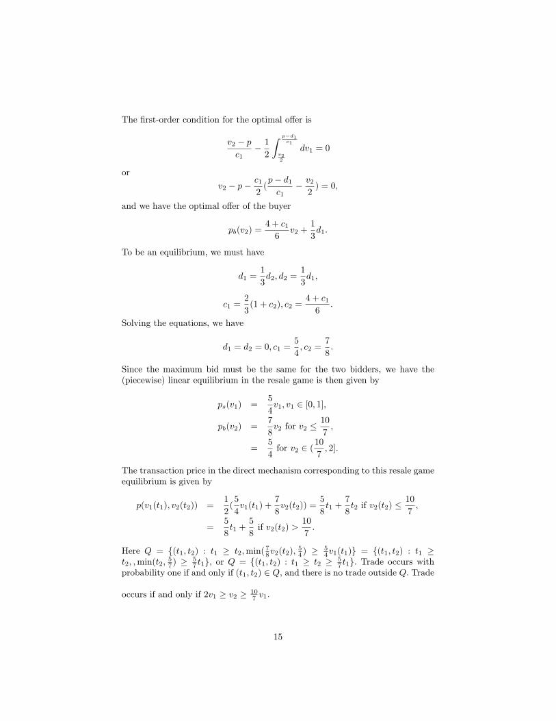
The transaction price in the direct mechanism corresponding to this resale gameequilibrium is given by

p(v1(t1); v2(t2)) =1

2(5

4v1(t1) +

7

8v2(t2)) =

5

8t1 +

7

8t2 if v2(t2) �

10

7;

=5

8t1 +

5

8if v2(t2) >

10

7:

Here Q = f(t1; t2) : t1 � t2;min(78v2(t2);

54 ) �

54v1(t1)g = f(t1; t2) : t1 �

t2; ;min(t2;57 ) �

57 t1g; or Q = f(t1; t2) : t1 � t2 � 5

7 t1g: Trade occurs withprobability one if and only if (t1; t2) 2 Q; and there is no trade outside Q: Trade

occurs if and only if 2v1 � v2 � 107 v1:

15

From Proposition 2, we get the equilibrium bidding strategies:

b1(t1) =1

t1

Z t1

0

w(t; t)dt =1

t1

Z t1

0

(5

8t+

7

8t)dt =

3

4t1; for t1 �

5

7

=1

t1

Z 57

0

3

2tdt+

1

t1

Z t1

57

(5

8t+

5

8)dt =

5

8(1 +

1

2t1 �

5

14t1); for t1 �

5

7

and the same formula applies to b2(t2): Hence

�1(b) = �2(b) =4

3b for b � 15

28:

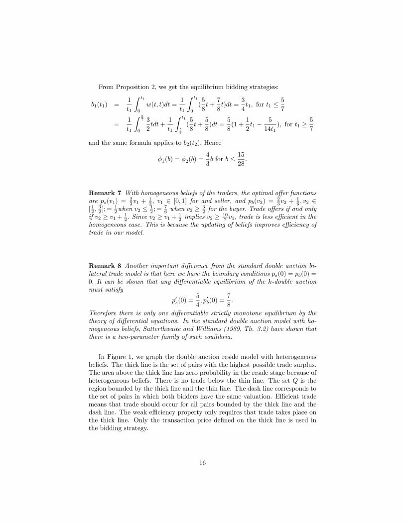
Remark 7 With homogeneous beliefs of the traders, the optimal o¤er functionsare ps(v1) = 2

3v1 +12 ; v1 2 [0; 1] for and seller, and pb(v2) =

23v2 +

16 ; v2 2

[ 12 ;32 ]; =

12when v2 �

12 ; =

76 when v2 �

32 for the buyer: Trade o¤ers if and only

if v2 � v1+ 12 : Since v2 � v1+

12 implies v2 �

107 v1; trade is less e¢ cient in the

homogeneous case. This is because the updating of beliefs improves e¢ ciency oftrade in our model.

Remark 8 Another important di¤erence from the standard double auction bi-lateral trade model is that here we have the boundary conditions ps(0) = pb(0) =0: It can be shown that any di¤erentiable equilibrium of the k-double auctionmust satisfy

p0s(0) =5

4; p0b(0) =

7

8:

Therefore there is only one di¤erentiable strictly monotone equilibrium by thetheory of di¤erential equations. In the standard double auction model with ho-mogeneous beliefs, Satterthwaite and Williams (1989, Th. 3.2) have shown thatthere is a two-parameter family of such equilibria.

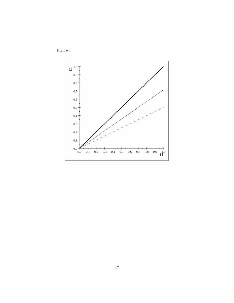
In Figure 1, we graph the double auction resale model with heterogeneousbeliefs. The thick line is the set of pairs with the highest possible trade surplus.The area above the thick line has zero probability in the resale stage because ofheterogeneous beliefs. There is no trade below the thin line. The set Q is theregion bounded by the thick line and the thin line. The dash line corresponds tothe set of pairs in which both bidders have the same valuation. E¢ cient trademeans that trade should occur for all pairs bounded by the thick line and thedash line. The weak e¢ ciency property only requires that trade takes place onthe thick line. Only the transaction price de�ned on the thick line is used inthe bidding strategy.

16

Figure 1

0.0 0.1 0.2 0.3 0.4 0.5 0.6 0.7 0.8 0.9 1.00.0

0.1

0.2

0.3

0.4

0.5

0.6

0.7

0.8

0.9

1.0

t1

t2

17

Figure 2

0.0 0.1 0.2 0.3 0.4 0.5 0.6 0.7 0.8 0.9 1.00.0

0.1

0.2

0.3

0.4

0.5

0.6

0.7

0.8

0.9

1.0

t1

t2

18

4 Bid Equivalence with two bidders

We assume that the pricing function p(v1(t1); v2(t2)) can be extended from Qto the set of all pairs (t1; t2) monotonically and smoothly so that the extensionis continuously di¤erentiable on the unit square. This extended function isdenoted by w(t1; t2): Consider a common-value auction in which the commonvalue is de�ned by w(t1; t2): From Theorem 1, we know that the equilibriumis the same for all di¤erent smooth monotonic extensions of p; as the biddingstrategy only depends on the value of w on the diagonal f(t; t) : t 2 [0; 1]g whichbelongs to Q by the weak e¢ ciency property.

The following bid equivalence result applies to all such extensions. Intuitivelythis says that the common value is de�ned by the transaction price in the resalegame when trade occurs with probability one. When there is possibility ofno trade, the common value can be de�ned arbitrarily without a¤ecting theequilibrium.

Theorem 9 Assume that there is no disclosure of bid information in betweenthe auction stage and the resale stage, and the resale process satis�es the weake¢ ciency property. Assume that there is a strictly monotone di¤erentiable equi-librium bidding strategy pro�le bi(t); i = 1; 2 in the auction with resale. Letw(t1; t2) be a monotonic extension of the the pricing function p(v1(t1); v2(t2))on Q, Then bi(t); i = 1; 2 is also an equilibrium of the common-value auctionwith the common value function w, and we have bid-equivalence between theauction with resale and the common-value auction.

Proof of Theorem 9:

From Proposition 2, the solution of the �rst-order condition gives us thesymmetric bidding strategy

bi(ti) =1

ti

Z ti

0

p(v1(s); v2(s))ds; ti > 0; bi(0) = 0: (6)

This strategy only depends on the value of w on the diagonal (t; t); hence isthe same for all monotonic smooth extension of p: According to Theorem 1,the equilibrium bidding strategy in (6) is an equilibrium of the common-valueauction.

For the proof in Theorem 1 to work, we require that the monotonic extensionto be smooth. It is convenient to allow the extension to have kinks. Becausethe equilibrium is una¤ected by di¤erent smooth extensions, we can use thosesmooth extensions to approximate a monotonic extension with possible kinks

19

and the equilibrium property holds in the limit. This means that the bid equiv-alence result still holds even if we allow the extension to have kinks.Kinked extensions are easier to describe. The following method is one way

to extend the de�nition of w to all pairs. For (t1; t2) outside Q; t2 < t1; letk1(t1) = infft2 : (t1; t2) 2 Qg: we de�ne w(t1; t2) = w(t1; k(t1)) for (t1; t2) =2 Q.For t2 > t1; we can just let w(t1; t2) = w(t2; t2): In this extension, we havekinks on the boundary of Q: We have the property w(t1; t2) � x when v1(t1) =v2(t2) = x:We can use the resale game example with simultaneous o¤ers in thelast section to illustrate the extension. On Q; we have

w(t1; t2) =5

8t1 +

7

8t2 if t2 �

5

7;

=5

8t1 +

5

8if t2 >

5

7:

For (t1; t2) =2 Q; t2 < 57 t1; we de�ne w(t1; t2) = w(t1;

57 t1) =

54 t1: If t2 > t1;

we let w(t1; t2) = w(t1; t1) =32 t1 when t1 �

57 ; and w(t1; t1) =

58 t1 +

58 when

t1 >57 : When v1(t1) = v2(t2) = x; we have t2 =

12 t1; and in this case, we have

w(t1; t2) =54 t1 =

54x > x:

Another alternative de�nition of the common value outside Q is to letk2(t2) = supft1 : (t1; t2) 2 Qg; and then de�ne w(t1; t2) = w(k2(t2); t2): In thisde�nition, we may have w(t1; t2) � x when v1(t1) = v2(t2) = x: For the sameexample, when (t1; t2) =2 Q; t2 < 5

7 t1, we de�ne w(t1; t2) = w( 75 t2; t2) =74 t2

when t2 � 57 : and w(

75 t2; t2) =

78 t2 +

58 when t2 >

57 : When v1(t1) = v2(t2) = x;

we have t2 = 12 t1; and in this case, we have w(t1; t2) =

74 t2 =

78x < x for

t2 � 57 :

In Figure 2, the extension of the price function outside Q can be de�nedas follows. The common value at any point on the lower part can be de�nedby going up vertically until a boundary point of Q is reached, and the trans-action price at that boundary point is the common value. At any point on theupper half, the common value can be de�ned by going right horizontally untila boundary point of Q is reached, and the transaction price at that boundarypoint is the common value.

In a bilateral trade equilibrium, trade need not occur with probability oneeven when the trade surplus is the highest possible amount. In this case, theweak e¢ ciency property fails, and the bid equivalence result need not hold.We shall give such an example with discrete valuations. Note that the abovebid equivalence result can be easily extended to the case of discrete valuations.To see this, assume that there are two bidders in an independent private-valueasymmetric auction. Bidder one valuation is either 0 or 1 with probability0:7 for 0: Bidder two valuation is either 0 or 2 with probability 0:4 for 0: Wecall bidder one the weak bidder, and bidder two the strong bidder. We canadopt a signal representation of the IPV model. This representation is calleda distributional approach) is �rst proposed in Milgrom and Weber (1985) anddiscussed extensively in Milgrom (2004). In this representation, both bidders

20

are described by step functions vi(ti) : [0; 1]! f0; 1];

v1(t1) = 0; when t1 2 [0; 0:7);= 1 when t1 2 [0:7; 1]

v2(t2) = 0; when when t1 2 [0; 0:5);= 1 when t1 2 [0:5; 1]

with the interpretation that vi(ti) is the private valuation of bidder i when he orshe receives the private signal ti: The two signals are assumed to be independent.The bidding strategies are mixed strategies which can be represented by

bi(ti); i = 1; 2: The inverse bidding function �i(b) is the cumulative bid distrib-ution of bidder i; i = 1; 2: The beliefs after the �rst-stage auction is describedconditional distribution of the signal tj over [0; �j(b)] when bidder i bids b andwins the auction. When bid i loses the auction after bidding b; the belief aboutbidder two is described by the conditional distribution of tj over [�j(b); 1]: Inthe space of valuations, such distributions are also discrete distributions. In thebilateral trade, a direct mechanism is a report of the signal rather valuation. Adirect trade mechanism then is represented by the probability of trade q(t1; t2);and the trade price p(t1; t2): Thus we can adopt the model with a continuum ofvaluations to the model with a continuum of signals. The �rst-order conditionof the equilibrium in the auction with resale holds except at ti when there is achange in valuation. The symmetry property continues to hold with the sameproof. The trading price on Q can be extended monotonically to the wholerange to de�ne a common value function. The equilibrium in the common-valueauction satis�es the same �rst-order condition except a �nite number of points.The equilibrium bidding strategy is given by the same formula, except that itis piecewise continuously di¤erentiable rather than continuously di¤erentiable.There is a bid equivalence between the equilibrium in the auction with resaleand the common value auction. For the example in the last paragraph, whenthe resale is a monopoly, the optimal monopoly price is 2 when bidder one winsthe auction: There is no resale if bidder two has valuation 0; or if bidder twowins the object and has valuation 2. The payo¤ of bidder one with valuation 1bidding b > 0 is

(�2(b)� 0:4)(2� b) + 0:4(1� b) = �2(b)(2� b)� 0:4:

The �rst-order condition for this maximization problem is

�02(b)(2� b)� �2(b) = 0;

or�02(b)

�2(b)=

1

2� b : (7)

For a bidder one with valuation 0; the payo¤ from bidding b > 0 is

(H2(b)� 0:4)(2� b) + 0:4(0� b) = H2(b)(2� b)� 0:8;

21

and the �rst-order condition is also (7): We have the same �rst-order conditionfor a bidder one with di¤erent valuations, because the resale opportunity haschanged his valuation to 2 rather than 0 or 1:For bidder two with valuation 2; there is no pro�t in the resale whether or

not there is resale. The payo¤ from bidding b > 0 is

H1(b)(2� b);

and the �rst-order condition is also given by

�01(b)

�2(b)=

1

2� b :

From the boundary conditions, �1(0) = 0:4 = �2(0); we get equilibrium9 inverse

bidding functions in the auction with resale:

�1(b) = �2(b) =0:8

2� b for b 2 [0; 1:2]:

and the equilibrium biding strategies

bi(t) = 2� 0:8twhen t � 0:4

= 0 when t � 0:4:

We have the set of trade

Q = f(t1; t2) : t1 < 0:4g\ [0:4; 1]�[0:4; 1]\f(t1; t2) : t1 � t2; 0 � ti � 1; i = 1; 2g:

and the pricing function on Q : p(t1; t2) = 0 if t1 < 0:4;= 2 if (t1; t2) 2 [0:4; 1]�[0:4; 1]: The common value function is a monotonic extension of p: For instance,we can have the extension w(t1; t2) = 0 if t1 < 0:4;= 2 if t1 � 0:4 for all pairsin [0; 1]� [0; 1]: The equilibrium bidding strategy of the common value functionis

bi(t) =1

t

Z t

0

p(s; s)ds =2

t(t� 0:4) = 2� 0:8

tif t � 0:4

= 0 if t < 0:4;

which is the same as the bidding strategy of the auction with resale.

Our counter example is a variation of the above example in which the resalemarket is a monopoly with trade impediments. This means that the winner ofthe auction makes o¤ers, but trade can only occur with probability 0:5 whenthe buyer accepts the o¤er. There is no trade when the buyer does not acceptthe o¤er. With this trade mechanism, the optimal o¤er by the seller is the sameas the monopoly price without restriction. Hence the optimal o¤er price is 2

9This equilibrium is unique for any tie-breaking rule adopted. In auctions with resale,bidder one with valuation 0 may bid positive amount because of future resale.

22

whenever there is a positive probability that the buyer has valuation 2. Let �idenote the equilibrium cumulative bid distribution of bidder i: The weak bidderwith valuation 1 chooses b to maximize the following payo¤

0:5(�2(b)�0:4)(2�b)+0:5(�2(b)�0:4)(1�b)+0:4(1�b) = �2(b)(1:5�b)�0:2:

The �rst-order condition is

�02(b)

�2(b)=

1

1:5� b : (8)

Bidder one with valuation 0 chooses b to maximize

0:5(�2(b)� 0:4)(2� b) + 0:5(�2(b)� 0:4)(0� b) + 0:4(0� b) = �2(b)(1� b)� 0:4

and the �rst-order condition is

�02(b)

�2(b)=

1

1� b : (9)

Bidder two with valuation 2 chooses b to maximize the payo¤

�1(b)(2� b)

with the �rst-order condition

�01(b)

�1(b)=

1

2� b : (10)

Let b� be the common maximum bid of both bidders. We have the followingboundary conditions

�2(0) = 0:4; �2(b�) = �1(b

�) = 1:

Note that the �rst-order conditions of the two bidders are not symmetric, and wedon�t expect the equilibrium bid distributions of the two bidders to satisfy thesymmetry property. If the symmetry property fails, then the equilibrium of theauction with this restricted monopoly resale market cannot be bid equivalentto any equilibrium of a common-value auction. To �nd the equilibrium, let�1(c) = 0:7: We have

�1(b) =A

2� b for b 2 [0; b�];

where A = 2� b�; 0:7(2� c) = 2� b�: For bidder two; we have

�2(b) =B

1:5� b for b 2 [c; b�];

hence B = 1:5� b�: For b 2 [0; c]; we must have �2(0) = 0:4; hence

�2(b) =0:4

1� b for b 2 [0; c]:

23

We must have

�2(c) =0:4

1� c =B

1:5� cor

0:4(1:5� c)1� c = B = 1:5� b� = 1:5� (2� 0:7(2� c)) = 0:9� 0:7c

We have the following quadratic equation in c :

(0:9� 0:7c)(1� c)� 0:4(1:5� c) = 0:7c2 � 1: 2c+ 0:3 = 0

and the solution is c = 0:303 86: From this number, we have b� = 0:687 30; A =1:31270; B = 0:81270: Hence we have the following equilibrium cumulative biddistributions when ties are broken in favor of bidder one:

�1(b) =1:3127

2� b ; b 2 [0; 0:6873];

�2(b) =0:4

1� b ; b 2 [0; 0:30386]

=0:8127

1:5� b ; b 2 [0:30386; 0:6873]:

Clearly, this equilibrium does not satisfy the symmetry property, and the bidequivalence result fails.

5 Buyer-Speculators Model of Auction with Re-sale

A special interesting case is worth mentioning here. Assume that group onehas only one member, and group two consists of n speculators. We refer to theonly group one member as bidder one and call it a regular buyer. A speculatorin group two has no value for the object, but participates in the auction forresale. We call this the buyer-speculators model of auction with resale. Assumethat the resale market is a monopoly. We shall extend our bid equivalenceresult in the last section to the buyer-speculators model. This means that theequilibrium bidding behavior of the buyer-speculators model is the same as theWilson Drainage Tract common value Model in which there is one neighborand n non-neighbors. The common value is the de�ned by the monopoly priceo¤ered by the winning speculator.

Consider an auction with resale model with n speculators indexed by i =2; :::; n + 1:and one regular buyer, Bidder one has a valuation function v(t)

24

over [0; 1]: Let bi(t) be the strictly increasing bidding strategy of bidder i and�i = b

�1i be the inverse. There is no resale if bidder one wins the auction, and

resale will occur if one of the speculators wins the auction. If bidder one withvaluation v(t) bids b; and loses the auction, the speculator i with highest bidwins the auction, and sells the object to bidder one. The price depends on �1(b)because the winning speculator believes that bidder one valuation is distributedover [0; �1(b)]: Let p(x) be the optimal monopoly price when the speculatormakes o¤ers to bidder one with valuation distributed over [0; x]: Let b� be the

maximum bid of all the speculators, G(b) =m+1Y�=2

�i(b): The pro�t of bidder one

can be written as

�R =

Z b�

b

[v(t)� p(v(�1(c)))] dG(c) +G(b)(v(t)� b):

The �rst-order condition is

G0(b)[p(v(�1(b)))� b]�G(b) = 0;

ord lnG(b)

db=

1

p(v(�1(b)))� b: (11)

For a speculator i = 2, the pro�t from bidding b is

nYj=3

�j(b) f[�1(b)� F (p(v(�1(b))))]p(v(�1(b)))� �1(b)bg :

Since the speculator uses a mixed strategy, it is pro�t is a constant which iszero when b = 0: Therefore the speculator has zero pro�t, and we have

[�1(b)� F (p(v(�1(b))))]p(v(�1(b)))� �1(b)b = 0: (12)

Let R(b) = [�1(b) � F (p(v(�1(b))))]p(v(�1(b))): By the envelop theorem, wehave

R0(b) = �01(b)p(v(�1(b)))

Taking the derivative of (12), we get

�01(b)[p(v(�1(b)))� b]� �1(b) = 0;

ord ln�1(b)

db=

1

p(v(�1(b)))� b: (13)

From the �rst-order conditions, we know that �1(b) = G(b): From this, we havethe bidding strategy

b1(t) =1

t

Z t

0

p(v(s))ds:

25

This is an equilibrium in the Wilson tract model with one neighbor and manynon-neighbors, and the common value is given by p(v(t1)) (see, for example,Milgrom (2004), Theorem 5.3.2). Therefore we have bid-equivalence betweenthe auction with resale and the Wilson tract model.It is an interesting question to ask whether bidders behave the same way in

both models in practice or in experiments10 . Given the evidence that winner�scurse is observed in many experiments in common-value auctions, it is interest-ing to see whether similar irrationality is observed in the auctions with resale.There is strong empirical support for the bidding behavior in the Wilson trackmodel. It is also promising that such support can be found in empirical studiesof auctions with resale.

6 Haile�s Resale Model

In the auctions with resale model of Haile (2000,2001,2003), bidders receivesignals in the �rst stage which are independent from each other, but are a¢ liatedwith their private values. In other words, before bidding, there is incompleteinformation about private valuation in the �rst stage. This uncertainty aboutprivate valuation is resolved in the second stage before resale occurs. The reasonfor resale is due the di¤erent realized private valuations in the second stage.This model is appropriate when there is dynamic discovery of information overtime. In our model, bidders know their private valuations before the biddingtakes place in the �rst stage. Thus asymmetry about valuation starts in thebeginning, and there is incentive for trade because the allocation of the objectneed not be e¢ cient in the �rst stage auction.The advantage of Haile�s auctions with resale model is that in the �rst stage

sealed-bid auctions, the bidding strategies are symmetric and easier to solvewhen the resale market is relatively simple. The disadvantage is that the up-dating of belief is more complicated. Bidders need to update their beliefs aboutthe signals received by their opponents in the �rst stage, as well as the realizedprivate valuation (the use value in Haile�s terminology) in the second stage. Theupdating is simpli�ed if the private valuations become common knowledge inthe second stage. In our model, it is di¢ cult to get explicit solutions to theasymmetric bidding behavior in the �rst stage in general even if the resale out-come is very simple. The updating of beliefs is simpler because it only involvesa change in the support of the private valuation, and the updated belief aboutthe opponents�private valuation is just the conditional distribution on the newsupport. When there are two bidders, we do get an explicit solution to the equi-librium bidding behavior in the �rst stage. Therefore the two ways of modelingauctions with resale are complementary to each other.We assume that there is no disclosure of bid information in our model, while

Haile assumed that all bids are disclosed and in his section 3 even the private

10Experiments based on the auction with resale model of Haile have been done in Lange,List, and Price (2004) for �rst-price auctions and Georganas (2008) for English auctions.

26

valuations are made common knowledge. In Haile�s model, the disclosure ofbids and valuations simpli�es the updating process, while in our model, the biddisclosure complicates the analysis, as it may eliminate the strictly increasingequilibrium bidding strategies (see Lebrun (2007) for an analysis with bid dis-closure). At the conceptual level, the di¤erent assumptions on bid disclosureonly lead to di¤erent updating and beliefs between the two stages. We takethe simplest information assumption to focus on the idea of bid equivalence. InHaile�s model, bid equivalence holds in a trivial way, as explained below. Fur-thermore, in his model, the connection between resale price and common valueis quite weak.There is no heterogeneity of beliefs in the resale stage in the Haile model.

This is because all bids are announced in his model, and beliefs in the secondstage are only a¤ected by the signals in the �rst stage. When the bids areannounced after the �rst-stage auction, the signals can be inferred, and becomecommon knowledge in the resale stage. Therefore a bidder�s belief about theopponent is independent of his revealed private valuation in the second stage.There is no signaling in our model as the deviation from bidding is not detectedwhen the bids are not disclosed. In Haile�s model, signaling is a feature of hismodel.We now give a brief description of the Haile (2003) model with two bidders

when the �rst stage is a �rst-price auction, and the resale mechanism is an op-timal auction (OA) conducted by the winner of the �rst stage auction. Eachbidder receives a signal si in the �rst stage, and the realized private valuationin the second stage is denoted by vi which is distributed according to a cumula-tive probability distribution G(vijsi) with the support [0; 1]: The signal si andvi are a¢ liated, but both are independent from sj ; vj of the other bidder. LetF (si) be the cumulative probability distribution of each si: Let �i = b�1i bethe inverse of the bidding strategy in the �rst stage. In the second stage, allbids are announced, and bidder i knows �j(bj) = sj ; hence believes that bidderj valuation has the distribution G(vj jsj): When bidder i wins the auction, hemakes an optimal monopoly o¤er to bidder j. Assume that there is complete in-formation in the second stage (as in section 3 of Haile (2003)). For each realizedvi 2 [0; 1]; all surplus is extracted from bidder j; and the revenue from the resaleisR 10(vi+

R 1vivjdG(vj jsj): Hence the expected revenue from the resale market for

bidder i with the signal si is wO(si; sj) =R 10

hR 10(vi +

R 1vivjdG(vj jsj)

idG(vijsi):

In the symmetric model of Haile, the bid equivalence holds in a trivial way. Anysymmetric equilibrium is an equilibrium of some common value auction. We canjust de�ne the common value as w(si; sj) = wO(min(si; sj); (si; sj)) for example:This common value is stochastically related to the transaction price as well asthe private valuation (when there is no trade), so that the connection betweentransaction price and common value is very weak. In our model, si = vi; and thecommon value is de�ned by the optimal monopoly price p(si; sj) whenever tradeis realized for the pair. Therefore, the bid equivalence result has clear meaningin our model. Furthermore, it is more useful because the bid equivalence leadsto identical bid distributions for asymmetric bidders.

27

In the Haile model with di¤erent auctions in the �rst stage or resale mech-anisms in the second stage, the same comments above apply. We still have bidequivalence, but the common value is only weakly connected to the resale price,and in general there is a combination of private and market valuations involvedin the �rst-stage equilibrium bidding strategy. For our model, only the trans-action price is involved in the equilibrium bidding strategy. Haile (2000,2003)also studied the implications of bargaining power and competition in auctionswith resale. Similar issues are investigated in Cheng and Tan (2008,2009) in ourframework.

7 Extension to the m-bidder Model

In this section, we shall assume that the winner of the �rst stage auction uses asecond-price auction in the second stage to sell the object to the losing bidders.The seller in the second-stage auction reserves the right to keep the objectto herself if the second highest bid is below her valuation. This amounts toa reservation price equal to the valuation of the seller in the second stage.Other reservation prices can be considered, and many of our results hold withmore general resale mechanisms. However, we shall deal with the simpler andimportant case of the second-price auctions here. An important property of thesecond-price auction is that it has the e¢ ciency property which is stronger thanany weak e¢ ciency conditions needed for resale mechanism in them bidder case.Another reason for considering the resale by the second price auction is that thecommon value function can be de�ned without reference to the bidding strategyin the �rst stage auction. This is not the case in Theorem 9. A comprehensivetreatment of the multiple bidder case is beyond the scope of this paper.

First we shall establish an important relationship between the common-valueauction and auction with resale in the symmetric model with many bidders. Itsays that the pro�t functions of the two auctions di¤er only by a constant (notdepending on bids). Since the optimal bid is determined by the maximizationof the pro�t function, the bid equivalence result follows easily from it. Thisproperty holds for asymmetric auctions, and will be shown for the case of twogroups of identical bidders. In fact, there is in some sense a strong tautologicalelement to the bid equivalence result.There are n � 3 identical bidders. The cumulative distribution of the val-

uations of each bidder is denoted by F (x) over [0; a]: Given a vector of valu-ations x = (x1; x2; :::; xn); let x�i denote the vector x without the xi compo-nent. Let x�1;i; i 6= 1 denote a vector without the component in 1 and i: Let

dG�i(x�i) =Yk 6=i

dF1(xk): Similarly, we let dG�1;i(x�1;i) =Yk 6=1;i

dF1(xk): Let

q(x) denote the second highest value among xi:Consider the common-value model in which si = xi: De�ne the common-

value function w(x) = q(x). We shall consider only symmetric equilibrium in

28

which all bidders use the same bidding strategy. Let �(b) be the inverse of thestrictly increasing bidding strategies b(xi) of each bidder. We have the followingproposition.

Proposition 10 Given �(:) of other bidders; and a bidder i with valuation x0bidding b; let �C(b); �R(b) be the pro�t function in the common-value auctionand the auction with resale (in the �rst stage) respectively. Then �R(b)��C(b)is independent of b; and is given by

�R(b)� �C(b) =Z x0Z0

[x0 �max(x�i)] dG�i(x�i):

Proof. Assume that bidder one has valuation x0; and bid b: The pro�t in the

common-value auction is

�C =

Z �(b)Z0

q(x0; x�1)dG�1(x�1)� bFn�1(�(b)):

Now consider the auction with resale. First assume that �(b) < x0:When bidderone wins the auction, there is no resale, and the revenue in the auction withresale is

R1 = x0Fn�1(�(b)):

If bidder one loses the auction, she buys from the winning bidder only if thewinning bidder has valuation lower than x0;and she has the highest valuationamong the losers. Therefore, in this case the revenue is

R2 = (n� 1)Z x0

�(b)

24Z xiZ0

[x0 � q(x0; x�1;i)] dG�1;i(x�1;i)

35 dF (xi)

= x0Fn�1(x0)�x0Fn�1(b)�

Z x0Z0

q(x0; x�1)dG�1(x�1)+

Z �(b)Z0

q(x0; x�1)dG�1(x�1):

Hence

�R��C = x0Fn�1(x0)�Z x0Z0

q(x0; z)dG�1(x�1) =

Z x0Z0

[x0�max(x�1)]dG�1(x�1):

Now assume that �(b) � x0: If bidder one wins the auction, there is resale ifone of the losing bidder has higher valuation than x0, and the revenue is

R1 = x0Fn�1(x0) + (n� 1)

Z �(b)

x0

24Z xiZ0

q(x0; x�1)dG�1;i(x�1;i)

35 dF (xi)29

= x0Fn�1(x0) +

Z �(b)Z0

q(x0; x�1)dG�1(x�1)�Z x0Z0

q(x0; x�1)dG�1(x�1):

When bidder one loses the auction, there is no resale and there is no revenue.Hence

�R��C = x0Fn�1(x0)�Z x0Z0

q(x0; x�1)dG�1(x�1) =

Z x0Z0

[x0�max(x�1)]dG�1(x�1):

Hence in either case, the Proposition holds.

From the Proposition, we have the following bid equivalence result.

Theorem 11 Assume that there are n identical bidders. In the resale stage, thewinner of the auction holds a second price auction to sell the object to the losingbidders. Then a strictly increasing bidding strategy b(:) is a symmetric equilib-rium of the common-value auction if and only if it is a symmetric equilibriumbidding strategy of the �rst stage of the auction with resale.

Proof. Let b(:) be a strictly increasing symmetric equilibrium bidding strategy

of the common-value auction. Since b (xi) maximizes �C ; it also maximizes�R; therefore, b(xi) is also an optimal bid in the auction with resale when allother bidders adopt the bidding strategy b(:): The converse holds by the sameargument.

Now we want to show the same result for asymmetric auctions with twogroup of bidders when the bidders in each group are identical in their valuations.Note that this proof is more general than the special arguments in the buyer-speculators model.

There are two groups of bidders, group one and two with m;n members re-spectively. Within each group, all bidders are identical. Consider the common-value model in which si = xi for group one and sj = yj : De�ne the common-value function w(x; y) = q(x; y) as the second highest valuation of all bidders.We want to establish the bid equivalence between the common-value auctionde�ned by this common value function and the auctions with resale model de-scribed above. We shall consider only equilibrium in which all bidders in thesame group use the same bidding strategy. Let �1(b); �2(b) be the inverse ofthe strictly increasing bidding strategies b1(xi); b2(xj) of group one, two biddersrespectively. We have the following bid equivalence result.

For convenience, we shall use the index i for group one, and index j forgroup two. Let x be a vector with valuations for group one and y be a vector

30

of valuations for group two, and z = (x; y) for a mixed vector. For any vector(possibly incomplete list) of valuations z; let max(z); q(z) be the highest, andsecond highest valuation among zk. Let x�i; y�j denote the vector x; y with-out the xi; yj component respectively. Let x�1;i denote a vector without thecomponent in 1 and i:Let dG�i(x�i) =

Yk 6=i

dF1(xk); dH(y) =Yj

dF2(yj): Similarly, we let dG�1;i(x�1;i) =Yk 6=1;i

dF1(xk); dH�j(y�j) =Yk 6=j

dF2(yk): We have the following result similar

to Proposition 10 for the symmetric case. The proof uses a similar idea, and isin the appendix.

Proposition 12 Given �1(:); �2(:); and a bidder i in group one with valuationx0 bidding b; let �C(b); �R(b) be the pro�t function of bidding b in the common-value auction and in the �rst stage of the auction with resale respectively. Then�R(b)� �C(b) is independent of b; and is given by

�R(b)� �C(b) =Z x0Z0

[x0 �max(x�i; y)] dG�i(x�i)dH(y):

Similar results hold for any bidder in group two.

By the same simple arguments of the symmetric case, we have the followingbid equivalence result.

Theorem 13 Assume that there are two groups of bidders. In each group, allbidders are identical. In the resale stage, the winner of the auction holds asecond price auction to sell the object to the losing bidders. Then a strictlyincreasing pair of bidding strategies b1(:); b2(:) is an equilibrium of the common-value auction if and only if it is an equilibrium pair of bidding strategies of the�rst stage of the auction with resale.

31

AppendixProof of Proposition 12:Without loss of generality, we can assume that bidder one in group one has

valuation x0: To simplify notations, let z = (x�1; y): For the common-value

auction, the net pro�t from bidding b is

�C =

Z �1(b)Z0

Z �2(b)Z0

q(x0; z)dG�1(x�1)dH(y)� bFn2 (�2(b))Fm�11 (�1(b)): (14)

For the auctions with resale model, to write down the formula for the pro�tfunction, we need to divide into di¤erent cases. Consider the casemin(�1(b); �2(b)) �x0: The revenue from the resale game is given by

R1 = x0Fm�11 Fn2 (x0)+(m�1)

Z �1(b)

x0

0@Z xiZ0

q(x0; z)dG�1;i(x�1;i)dH(y)

1A dF1(xi)+n

Z �2(b)

x0

0@Z yjZ0

q(x0; z)dG�1(x�1)dH�j(y�j)

1A dF2(yj)= x0F

m�11 Fn2 (x0)+

Z �1(b)Z0

Z �2(b)Z0

q(x0; z)dG�1(x�1)dH(y)�Z x0Z0

q(x0; z)dG�1(x�1)dH(y)

= x0Fm�11 Fn2 (x0)�

Z x0Z0

max(z)dG�1(x�1)dH(y)+

Z �1(b)Z0

Z �2(b)Z0

q(x0; z)dG�1(x�1)dH(y)

(15)If she loses the auction, there is no resale, and R2 = 0.

From (3) and (14), we have

�R � �C =Z x0Z0

[x0 �max(z)] dG�1(x�1)dH(y): (16)

Now consider the case max(�1(b); �2(b)) < x0: There is no resale if she winsthe auction, hence

R1 = x0Fm�11 (�1(b))F

n2 (�2(b)):

If she loses the auction, she buys from the winning bidder only if she has thehighest valuation among the losers. The revenue is

R2 = (m� 1)Z x0

�1(b)

24Z xiZ0

[x0 � q(x0; z)] dG�1;i(x�1;i)dH(y)

35 dF1(xi)32

+n

Z x0

�1(b)

24Z yjZ0

[x0 � q(x0; z)] dG�1(x�1)dH�j(y�j)

35 dF2(yj)= x0F

m�11 (x0)F

n2 (x0)�x0Fm�11 (�1(b))F

n2 (�2(b))+

Z �1(b)Z0

Z �2(b)Z0

q(x0; z)dG�1(x�1)dH(y)

�Z x0Z0

q(x0; z)dG�1(x�1)dH(y)

=

Z x0Z0

[x0�max(z)]dG�1(x�1)dH(y)+Z �1(b)Z

0

Z �2(b)Z0

[q(x0; z)�x0]dG�1(x�1)dH(y)

Therefore we have

�R =

Z x0Z0

[x0�max(z)]dG�1(x�1)dH(y)+Z �1(b)Z

0

Z �2(b)Z0

[q(x0; z)�b]dG�1(x�1)dH(y)

and we have (16) in this case as well.Now consider the case �1(b) < x0 � �2(b): In this case when bidder one wins

the auction, she only sells to the bidders in group two. If she loses the auction,she only buys it from bidders in group one. Hence we have

R1 = x0Fm�11 (�1(b))F

n2 (x0)+nF

m�11 (�1(b))

Z �2(b)

x0

0@Z yjZ0

q(x0; y)dH�j(y�j)

1A dF2(yj);

= x0Fm�11 (�1(b))F

n2 (x0)+n

Z �2(b)

x0

0B@Z �1(b)Z0

Z yjZ0

q(x0; z)dG�1(x�1)dH�j(y�j)

1CA dF2(yj)

= x0Fm�11 (�1(b))F

n2 (x0) +

Z �1(b)Z0

Z �2(b)Z0

q(x0; z)dG�1(x�1)dH(y)

�Z �1(b)Z

0

Z x0Z0

q(x0; z)dG�1(x�1)dH(y)

R2 = (m� 1)Z x0

�1(b)

24Z xiZ0

[x0 � q(x0; z)] dG�1;i(x�1;i)dH(y)

35 dF1(xi)= x0F

n2 (x0)[F

m�11 (x0)�Fm�11 (�1(b))]�(m�1)

Z x0

�1(b)

24Z xiZ0

q(x0; z)dG�1;i(x�1;i)dH(y)

35 dF1(xi)33

= x0Fn2 (x0)[F

m�11 (x0)� Fm�11 (�1(b))]�

Z x0Z0

q(x0; z)dG�1(x�1)dH(y)

+

Z �1(b)Z0

Z x0Z0

q(x0; z)dG�1(x�1)dH(y)

We have

�R = x0Fm�11 (x0)F

n2 (x0) +

Z �1(b)Z0

Z �2(b)Z0

q(x0; z)dG�1(x�1)dH(y)

�Z x0Z0

max(z)dFm�11 (x�1)dFn2 (y)� bFm�11 (�1(b))F

n2 (�2(b))

and we again have (16) in this case as well. The last case �2(b) < x0 � �1(b) iscompletely similar. In all cases, the di¤erence between the two pro�t functionsis independent of b: The above proof is applicable to any bidder in group one ortwo.

34

References:Ashenfelter, O. and D. Genesove (1992), "Testing for price anomalies in

real-estate auctions", Amer. Econom. Rev. 82, 501�505.Bikhchandani, Sushil and Huang, Chi-fu (1989), "Auctions with Resale Mar-

kets: An Exploratory Model of Treasury Bill Markets." Review of FinancialStudies, 2(3), pp. 31 1-39.Chakravorti, B., R. E. Dansby, W. W. Sharkey, Y. Spiegel, and S. Wilkie

(1995), "Auctioning the airwaves: the contest for broadband PCS spectrum",J. Econom. Management Strategy 4, 345�373.Chatterjee, Kalyan and William Samuelson (1983), �Bargaining Under In-

complete Information,�Operations Research, 31, 835-851.Cheng, H. and Guofu Tan (2008), "Asymmetric Common Value auctions

and Applications to Auctions with Resale," mimeo. Department of Economics,University of Southern California.Cheng, H. and Guofu Tan (2009), "Auctions with Resale and Bargaining

Power," Department of Economics, University of Southern California.Cramton, P.C. (1995), "Money out of thin air: the nationwide narrowband

PCS auction", J. Econom. Management Strategy 4, 267�343.Gale, I., D. B. Hausch, and M. Stegeman (2000), "Sequential procurement

with subcontracting", Internat. Econom. Rev. 41, 220�989.Garratt, R., Thomas Troger, and Charles Zheng (2007), "Collusion via Re-

sale", mimeo. Department of Economics, U.C. Santa Barbara.Georganas, Sotirios (2008), "English Auctions with Resale: An Experimental

Study," April 2008, Department of Economics, Ohio State University.Green, J. and J.-J. La¤ont (1987), "Posterior Implementability in a Two-

Person Decision Problem," Econometrica 55, 69-94.Gupta, M. and B. Lebrun (1999), �First Price Auctions with Resale,�Eco-

nomic Letters 64: 181-185.Georganas, S. and J. Kagel (2009), "Asymmetric Auctions with Resale: an

experimental study," Department of Economics, Ohio State University.Hafalir, I., and V. Krishna (2008), �Asymmetric Auctions with Resale,�

American Economic Review 98, no.1, 87-112.Haile, P. (2000), "Partial Pooling at the Reserve Price in Auctions with

Resale Opportunities." Games and Economic Behavior, November 2000, 33(2),pp. 231-48.Haile, P. (2001), �Auctions with Resale Markets: An Application to U.S.

Forest Service Timber Sales,�American Economic Review 91: 399-427.Haile, P. (2003), "Auctions with Private Uncertainty and Resale Opportu-

nities," Journal of Economic Theory 108, 72�110Haile, P., Hong, H., and Shum, M., (2003), "Nonparametric Tests for Com-

mon Values in First-Price Sealed-Bid Auctions," mimeo.Hausman, and J., D. Wittman, Analysis and recommendations for FCC PCS

spectrum auctions, Attachment to Comments of Pactel, FCC PP Docket, 1993,pp. 93�253.Hortascu, A. and J. Kastl (2008), "Testing for Common Valuation in the

Presence of Bidders with Informational Advantage," working paper presented

35

at the Penn State auctions conference, April 2008.Kagel, John H. and Dan Levin (2002), Common Value Auctions and the

Winner�s Curse, Princeton University Press, Princeton and Oxford.Kamien, M.I., L. Li, and D. Samet (1989), "Bertrand competition with

subcontracting", Rand J. Econom. 20, 553�567.Lange, Andreas, John A. List, Michael K. Price (2004), "Auctions with

Resale When Private Values Are Uncertain: Theory and Empirical Evidence",NBER Working Paper No. w10639Klemperer, P. (2004), Auctions: Theory and Practice, Princeton University

Press.Lebrun, B. (2007), �First-Price and Second-Price Auctions with Resale,�

working paper, Department of Economics, York University, Toronto, Canada.Maskin E. and J. Riley (2000), �Asymmetric Auctions�, Review of Economic

Studies 67: 413-438.McAfee, R. P. and J. McMillan (1987), "Auctions and bidding", J. Econom.

Lit. 25, 669�738.McMillan, J. (1994), "Selling spectrum rights, J. Econom. Perspect. 8,145�

162.Milgrom, P.R. (1987), "Auction theory", in: T.F. Bewley (Ed.), Advances

in Economic Theory: Fifth World Congress, Cambridge University Press, Cam-bridge, pp. 1�32.Milgrom, P. (2004), Putting Auction Theory to Work, Cambridge University

Press.Milgrom, P., and R. Weber (1982), �A Theory of Auctions and Competitive

Bidding,�Econometrica 50: 1089�1122.Milgrom, P., and R. Weber (1985), �Distributional Strategies for Games with

Incomplete Information,�Mathematics of Operations Research 10: 619-632.Myerson R.B. and M.A. Satterthwaite (1983), "E¢ cient Mechanisms for

Bilateral Trading," Journal of Economic Theory 29, 265-81.Plum, M. (1992): �Characterization and Computation of Nash Equilibria for

Auctions with Incomplete Information,�International Journal of Game Theory,20, 393�418.Parreiras, S. (2006), �A¢ liated Common Value Auctions with Di¤erential

Information: The Two Buyer Case�, forthcoming in the B.E. Journals in The-oretical Economics.Rosenthal, R.W., and R. Wang (1996), "Simultaneous auctions with syner-

gies and common values", Games Econom. Behav. 17, 32�55.Rothkopf, M.H., and R. M. Harstad (1994), "Modeling competitive bidding:

a critical essay", Management Sci. 40, 364�384.Satterthwaite M. and S. Williams (1989), "Bilateral Trade with the Sealed

Bid k-Double Auction: Existence and E¢ ciency", Journal of Economic Theory48, 107-133.U.S. Forest Service (1976), Forest service manual, Amendment 95, Title

2400, Washington, DC: U.S. Department of Agriculture, May 1976.U.S. Forest Service (1981), Forest service manual, Amendment 123, Title

2400, Washington, DC: U.S. Department of Agriculture, February 1981.

36

Williams, Steve (1987), "E¢ cient Performance in Two Agent Bargaining,"Journal of Economic Theory 41, 154-172

37