Private versus public monopoly

Jörgen Weibull and Jun Chen∗

December 20, 2016

Abstract

We compare private and public monopoly with respect to how much resourcesthey spend on finding out what product varieties people want. We propose a sim-ple model in which a monopolist supplies one variety of a good. This variety ischosen by the monopolist and consumers differ in their valuations of the goodand preferences over product varieties. The monopolist does not know the pref-erence distribution, but can, at a cost, acquire more or less precise informationabout this distribution. We analyze the monopolist’s endogenous informationacquisition and choice of product variety in the following three scenarios: anunregulated profit-maximizing monopolist, the first-best welfare solution, and amonopolist who maximizes a convex combination of profit and welfare under abudget constraint. Our main finding is that, broadly speaking, public monopolyis preferable in societies with a wide spread in income and/or wealth while pri-vate monopoly is better in societies with less inequity.

Keywords: Uncertainty, information acquisition, monopoly, Boiteux-Ramseyprice, regulation, inequity.JEL Classification: D21, D42, D60, L12, L51

1 Introduction

We here address the following question: Does a monopolist make too little, just aboutright, or too much - from a welfare point of view - to find out what product varietiesconsumers want? We posit a simple model in which a monopolist chooses a product

∗Weibull: Department of Economics, Stockholm School of Economics, Department of Mathematics,KTH Royal Institute of Technology, and Institute for Advanced Study in Toulouse. Chen: Departmentof Economics, Stockholm School of Economics. The authors are grateful for comments from FrancoisSalanié, Xavier Vives, Paul Segerstrom, Jens Josephson and Chloé Le Coq. A preliminary versionwas circulated under the title "How interested is a monopolist in consumer preferences?". Financialsupport from Knut and Alice Wallenberg Research Foundation is gratefully acknowledged.

1

variety, from a continuum range, to supply to the market. Consumers have idiosyn-cratic Euclidean preferences over product varieties, and differ in their willingness topay. For example, one rich individual may prefer a certain variety x and is willingto pay a lot for this personal ideal variety, while another, poor, individual may pre-fer a variety y (which may or may not be the same as x ), but is willing to pay lessfor her personal variety. The monopolist does not know the preference distributionin the population. It only has a vague prior belief about it. However, the monopo-list may, at a cost, choose to obtain more precise information, where higher precisioncosts more. We represent the monopolist’s information about demand as a noisy sig-nal about some parameter in the preference distribution. The monopolist may be anunregulated profit maximizer, an unconstrained welfare maximizer ("first-best"), or,more generally, it may have a goal function that is an arbitrary convex combinationof profit and welfare.

This paper belongs to the small literature dealing with firms’ choice of price andlocation, or product variety, under uncertainty (see Vives, 1984; Harter, 1997; Casado-Izaga, 2000; Meagher and Zauner, 2004, 2005, 2011; Król, 2012). While all of thosepapers deal with duopoly under exogenous uncertainty, we here analyze monopolyunder endogenous uncertainty.1 The paper most closely related to us is Meagher(1996). However, that paper does not address the question of optimal informationacquisition. Instead, it considers a dynamic environment in which consumer pref-erences change over time and are not directly observable, and where the firm canconduct market research.

We proceed to first analyze an unregulated profit-maximizing monopolist’s infor-mation gathering, price setting and choice of product variety (or location). Secondly,we perform the same analysis on an unconstrained welfare-maximizing monopolist,where welfare is defined as the sum of profit and consumer surplus. Such a monop-olist will finance its activity by a lump-sum tax on all citizens. Third, and last, weanalyze a monopolist who maximizes expected welfare under the constraint that itsexpected profit reaches an arbitrary pre-specified level. This setting is in line with theclassical Ramsey-Boiteux approach (see Ramsey, 1927; Boiteux, 1971), and we obtainresults for a wide range of second-best cases.

In our simple model, the monopolist’s choice of product variety, at any given levelof its uncertainty about consumer preferences, is always socially efficient; irrespectiveif its goal is profit or welfare or some convex combination thereof, the monopolist al-ways strives to supply a variety that will attract as many consumers as possible, at

1In this paper we assume that consumers know their own valuations of the product. If consumersdo not know their valuations, the monopolist’s pricing may convey information to the consumersand there may be multiple equilibria. Furthermore, if consumers can acquire costly information, thenthe price in equilibrium might not be perfectly informative. See Bester and Ritzberger (2001) and thereferences therein. If there are more than one firm in the market, and the consumes do not know thequality or the valuation of the product, consumers’ information acquisition choice may endogenizethe trading rules, see Bester (1993) for an inference.

2

any given price. By contrast, the different types of monopoly differ in the extentof their information acquisition. An unregulated profit-maximizing monopolist willtypically either spend too little or too much resources on information acquisition,compared with first-best. The wider is the dispersion of consumers’ valuations oftheir ideal product varieties, the further is the unregulated private monopoly fromfirst-best information acquisition. In a society with a wide spread in valuations,the unregulated private monopolist therefore underinvests in information acquisi-tion about consumer preferences, while in societies with little spread in valuationsit overinvests, compared to first-best. It is only at an intermediate knife-edge caseof dispersion of valuations that an unregulated private monopolist achieves the firstbest. Broadly speaking, public or regulated private monopoly is preferable in so-cieties with a wide dispersal of valuations, as would be expected in societies witha wide spread in income and/or wealth (say, India). By contrast, in societies withmodest spread in valuations, such as would be expected in societies with fairly equaldisposable incomes or wealth (say, Sweden), private monopoly is better than publicmonopoly. Our paper thus also relates to the literature on monopoly regulation, seeArmstrong and Sappington (2007).

In this study of monopoly, we neglect many important aspects. Perhaps the mostglaring omission is that this study presumes that the management of the monopoly,whether private or public, is fully rational and does not (try to) extract any privaterents, such as shirking from work, taking bribes, using funds for luxurious offices,extravagant dinners, expensive but ill-motivated trips etc. Our focus is entirely onthe monopolist’s incentives to acquire information about consumer tastes. To the bestof our knowledge, this is the first paper studying this aspect of monopoly behavior.

We begin by setting up the model in Section 2. In Section 3 we analyze the caseof an unregulated private monopolist. Here, the monopolist strives to maximize itsexpected profit, defined as its revenue from sales, net of production costs and its costsfor information acquisition about consumer preferences over product varieties (or lo-cations). In Section 4 we consider the first-best case of a monopolist who strives tomaximize expected social welfare, defined as the sum of its profit and consumer sur-plus, without any budget constraint. In Section 5 we consider a range of intermediatecases, between the previous two extremes, and obtain the second-best solution, thatof a monopolist who strives to maximize expected social welfare under a budget con-straint. All numerical results are shown in Section 6. Section 7 briefly discusses somepotential extensions of the model and Section 8 concludes.

2 Model

Consider, thus, a monopolist in a market for a differentiated good sold in indivisibleunits. The monopolist has to choose a product variety x ∈ X = R and a price p ∈ R+

3

for this variety. The monopolist has a constant unit production cost c ≥ 0. In thisanalysis, we abstract from fixed production costs. There is a continuum of consumers,each with unit demand for the good. Every consumer has Euclidean preferencesover varieties, with a personal ideal product-variety θ ∈ X. A consumer type is apair τ = (θ, v) ∈ X × V, where V is an interval. The utility for a consumer of typeτ = (θ, v) from buying one unit of product variety x at price p is

u = Uτ (x, p) = v− p− (θ − x)2 (1)

We will refer to v ∈ V as the consumer type’s valuation (of its ideal product variety).The utility from not buying is normalized to zero. A buyer of type τ buys a unit ifand only if Uτ (x, p) ≥ 0.

Each consumer’s type τ is his or her private information. The population is treatedas a continuum with unit mass, and v and θ are treated as statistically independentrandom variables. Hence, there is no correlation between a consumer’s valuation andhis or her product ideal. The cumulative distribution function (CDF) for valuations, v,is denoted F : V → [0, 1], where F is absolutely continuous with density f : V → R+

and such that the mean value E [v] exists and exceeds the unit production cost c:

c < v = E [v] < +∞

Each consumer’s ideal product variety, θ, is the sum of a shared component, θ0,common to all consumers in the population, and an idiosyncratic component (drivenby fashion or social norms), ξ:

θ = θ0 + ξ (2)

These two components are statistically independent and normally distributed, bothwith mean-value zero. The shared component, θ0, has variance 1/α > 0 and the id-iosyncratic component, ξ, has variance 1/β > 0. Aggregate demand for each productvariety x is thus given by the demand function D : R×R+ → R+ defined by

D (x, p) =∞∫

p

Pr[x−

√v− p ≤ θ ≤ x +

√v− p

]f (v) dv (3)

The integrand represents the mass of willing consumers for each valuation v. Thisis illustrated in Figure 1 below. The area above the parabola is the set of "willingconsumer types" when the price is at the horizontal dashed line and the suppliedvariety at the vertical dashed line. The monopolist’s revenue from sales is thus itsprice multiplied by the population mass of willing consumers, those with types insidethe parabola.

The monopolist knows all of the above. In addition, it can, at a cost, acquire moreinformation about the shared component, θ0, of consumer preferences over product

4

θ

v

v = p + (θ − x)2

x

p

Figure 1: The set of willing buyers

varieties.2 We represent such information as a signal

s = θ0 + ε

where the error (or noise) term ε is statistically independent of all other random vari-ables and is normally distributed with mean-value zero and variance 1/q, where theprecision q ≥ 0 is chosen by the monopolist, with q = 0 representing "no infor-mation acquisition" or "no signal". The cost for signal precision q is C (q), whereC : R+ → R+ is twice differentiable with C (0) = C′ (0) = 0, C′, C′′ > 0 andC′ (q) > 0 for all q > 0.

The time-line is as follows: the monopolist first chooses its signal precision, thenobserves the signal realization s and thereafter chooses its product variety x and aprice p. After these events, consumers observe the monopolist’s product variety andprice, sales occur and profits and utilities are realized. A strategy for the monopolistis a signal precision and, given any signal precision and any subsequently observedsignal value, a product variety and price. Formally, a strategy is a pair 〈q, ψ〉, whereq ∈ R+ and ψ : R+ ×R→ R×R+ assigns to each precision-signal pair (q, s) somevariety-price pair (x, p).

For any signal precision q, signal value s, product variety x and price p, let E(q,x,p)[Π |s] be the monopolist’s posterior expected profit (after the signal has been received), andlet E(q,x,p) [W | s] be the posterior expected welfare, where welfare is defined as con-sumer surplus plus monopoly profit. Let E(q,ψ) [Π] and E(q,ψ) [W] be the associatedex ante expected profit and welfare (before the signal is received) under strategy 〈q, ψ〉,defined by

E(q,ψ) [Π] = E(

E(q,ψ1(q,s),ψ2(q,s)) [Π | s])

2In order to keep focus on consumer preferences over varieties, we do not endogenize the monop-olist’s information about the consumer valuation distribution.

5

andE(q,ψ) [W] = E

(E(q,ψ1(q,s),ψ2(q,s)) [W | s]

)The monopolist’s goal is to maximize a convex combination of these two latter expec-tations. Formally, it solves the optimization program

max〈q,ψ〉

(1− γ)E(q,ψ) [Π] + γE(q,ψ) [W] (4)

where γ ∈ [0, 1] is an exogenous parameter. At one end of the parameter spectrum,γ = 0, we find the unregulated profit-maximizing monopolist while at the oppositeend of the spectrum, γ = 1, we find the welfare-maximizing monopolist, the monop-olist that implements the first-best solution (in terms of welfare). As will be shownbelow, for an intermediate parameter value, 0 < γ < 1, we will find the second-best public monopoly, that is a welfare-maximizing monopolist that faces the budgetconstraint that its ex ante expected profit be non-negative.

We note that optimality in Equation (4) requires that the monopolist’s choice ofproduct variety and price be optimal after (almost) all possible signal realizations.3

We also note that, since we have normalized the consumer population to unity, all ex-pected values above are bounded from below by −c and from above by consumers’average valuation, v, of their ideal product varieties minus the marginal cost of pro-duction. The latter claim follows from the observation that in the "best of worlds"production costs are nil and each consumer obtains his or her ideal product varietyfor free, in which case E [W] = v− c. Hence, in general

E(q,ψ) [Π] ≤ E(q,ψ) [W] ≤ v− c

We proceed to first analyze the case γ = 0, then the case γ = 1, and finally turnto all intermediate cases γ ∈ (0, 1). Henceforth, let Φ denote the CDF of the standardnormal distribution N (0, 1) and let φ be its density.

3 Unregulated profit maximization

We here consider an unregulated profit-maximizing monopolist; the case γ = 0. Op-timality in Equation (4) requires that the monopolist’s choice of product variety andprice be optimal after (almost) all possible signal realizations.

Suppose that the monopolist has chosen signal precision q and observed a signalvalue s, and is about to choose a product variety and price. In such a situation, the

3Since the signal by assumption has an absolutely continuous probability distribution, the goalfunction is unaffected by deviations from optimality on any subset of signal values with Lebesquemeasure zero.

6

monopolist will strive to maximize its conditionally expected profit,

E(q,x,p) [Π | s] = (p− c) ·∞∫

p

Pr[x−

√v− p ≤ θ ≤ x +

√v− p | s

]f (v) dv

− C (q)

(5)

This is the net earnings per unit sold, p − c, multiplied by the mass of willing con-sumers, minus the monopolist’s information costs to obtain signal precision q. How-ever, at this decision stage, the latter costs are sunk, so the last term is irrelevant forthe monopolist’s choice of product variety and price. The following result establishesthat the monopolist’s choice of product variety is a random variable that dependslinearly on the signal, while its price is deterministic and independent of the signalvalue. Moreover, we find that the choice of product variety is more sensitive to thesignal the higher its precision. In particular, if the monopolist has (previously) chosento acquire no information, q = 0, then it will opt for product variety x = 0, the ex anteexpected mean value of consumers’ ideal product variety.

PROPOSITION 1. For any signal precision q ≥ 0 and any observed signal value s ∈ R,the profit-maximizing monopolist (γ = 0) will choose product variety

x∗ =q

α + q· s (6)

and set its price p∗ so that

p∗ ∈ arg maxp≥0

(p− c) ·∞∫

p

[Φ

(√(α + q) (v− p) β

α + β + q

)− 1

2

]f (v) dv (7)

Moreover, the set on the right-hand side of Equation (7) is a non-empty and compact subset ofthe open interval (c,+∞).

Proof: Conditional upon an observed signal value s, the monopolist’s posteriorfor θ0 is normally distributed,

θ0 |s ∼ N(

qsα + q

,1

α + q

)By assumption, the idiosyncratic taste parameter ξ is statistically independent of bothθ0 and s, so ξ |s ∼ ξ ∼ N (0, 1/β) and thus

θ |s ∼ N(

qsα + q

,1

α + q+

1β

)

7

The conditional random variable θ |s is symmetrically and unimodally distributedaround its mean-value, µ = sq/ (α + q), so for any p ≥ 0, the monopolist will choosea product variety x such that, for any valuation v ∈ V, the associated interval of "will-ing buyer types", θ ∈ [x−√v− p,x +

√v− p], is centered on µ. Hence, it is optimal

for the monopolist to select product variety x∗ as given in Equation (6). Given thischoice of product variety, and conditional upon the realized signal s, the monopolistchooses its price p so as to maximize

p− cσθ

√2π·

∞∫p

µ+√

v−p∫µ−√v−p

exp

[−1

2

(t− µ

σθ

)2]

dt

f (v) dv

where σ2θ = (α + β + q) /[(α + q) β] is the variance of θ |s . After a change of variables

one obtains Equation (7). The maximand in Equation (7) is a continuous functionof p that vanishes at p = c and as p → +∞.4 Moreover, the maximand is positiveat intermediate values of p. Hence, by Weierstrass’ maximum theorem, the set ofmaximizers is a non-empty and compact subset of the open set V. Q.E.D.

Hence, the monopolist’s optimal variety/price strategy ψ∗ = (ψ∗1 , ψ∗2) satisfiesψ∗1 (q, s) = qs/ (α + q) for all q ≥ 0 and all s ∈ R, and ψ∗2 is constant across signalvalues, ψ∗2 (q, s) = ψ∗2 (q, s′) for all q ≥ 0 and s, s′ ∈ R. We will henceforth thus writep∗ (q) for ψ∗2 (q, s). Since every optimal price is interior (with respect to the support ofthe valuation distribution), the price p has to satisfy the first-order condition that thederivative of the maximand in Equation (7) with respect to p, is zero. This conditionin fact uniquely determines the pricing strategy p∗ : R+ → R+, to be specified in thenext result. Let

η (q) =

√(α + q) β

α + β + q(8)

This is the square root of the precision of the posterior (after the signal) estimate ofindividuals’ ideal product varieties.

4To see that the maximand tends to zero as p tends to plus infinity, write the maximand as m (p)and note that

m (p) ≤ p∫ +∞

pg (v) dv ≤

∫ +∞

pvg (v) dv

Since v < +∞, the last integral has to converge to zero as p→ +∞. To see the latter claim, note that

v =∫ p

0vg (v) dv +

∫ +∞

pvg (v) dv ∀p > 0

where the first integral converges to v as p→ +∞.

8

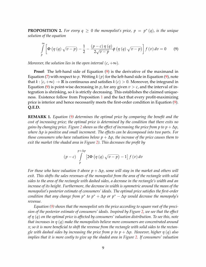
PROPOSITION 2. For every q ≥ 0 the monopolist’s price, p = p∗ (q), is the uniquesolution of the equation

∞∫p

[Φ(η (q)

√v− p

)− 1

2− (p− c) η (q)

2√

v− pφ(η (q)

√v− p

)]f (v) dv = 0 (9)

Moreover, the solution lies in the open interval (c,+∞).

Proof: The left-hand side of Equation (9) is the derivative of the maximand inEquation (7) with respect to p. Writing k (p) for the left-hand side in Equation (9), notethat k : [c,+∞)→ R is continuous and satisfies k (c) > 0. Moreover, the integrand inEquation (9) is point-wise decreasing in p, for any given v > c, and the interval of in-tegration is shrinking, so k is strictly decreasing. This establishes the claimed unique-ness. Existence follow from Proposition 1 and the fact that every profit-maximizingprice is interior and hence necessarily meets the first-order condition in Equation (9).Q.E.D.

REMARK 1. Equation (9) determines the optimal price by comparing the benefit and thecost of increasing price; the optimal price is determined by the condition that there exits nogains by changing price. Figure 2 shows us the effect of increasing the price from p to p+∆p,where ∆p is positive and small increment. The effects can be decomposed into two parts. Forthose consumers who have valuations below p + ∆p, the increase of the price causes them toexit the market (the shaded area in Figure 2). This decreases the profit by

(p− c)

p+∆p∫p

[2Φ(η (q)

√v− p

)− 1]

f (v) dv

For those who have valuation v above p + ∆p, some will stay in the market and others willexit. This shifts the sales revenues of the monopolist from the area of the rectangle with solidsides to the area of the rectangle with dashed sides, a decrease in the rectangle’s width and anincrease of its height. Furthermore, the decrease in width is symmetric around the mean of themonopolist’s posterior estimate of consumers’ ideals. The optimal price satisfies the first-ordercondition that any change from p∗ to p∗ + ∆p or p∗ − ∆p would decrease the monopoly’srevenue.

Equation (9) shows that the monopolist sets the price according to square root of the preci-sion of the posterior estimate of consumers’ ideals. Inspired by Figure 2, we see that the effectof η (q) on the optimal price is affected by consumers’ valuation distribution. To see this, notethat increases in η (q) make the monopolists believe more consumers are concentrated aroundx; so it is more beneficial to shift the revenue from the rectangle with solid sides to the rectan-gle with dashed sides by increasing the price from p to p + ∆p. However, higher η (q) alsoimplies that it is more costly to give up the shaded area in Figure 2. If consumers’ valuation

9

θ

v

v = p + (θ − x)2

v = p + ∆p + (θ − x)2

x

p

p + ∆p (p− c)p+∆p∫

p[2Φ(η(q)

√v− p)− 1] f (v)dv

v

c

(p + ∆p− c)[2Φ(η(q)√

v− p− ∆p)− 1]

(p− c)[2Φ(η(q)√

v− p)− 1]

Figure 2: The effect of increasing price

is very concentrated around p in Figure 2, it is very costly for the monopolist to give up theshaded area; in this case, increases in η (q) force the monopolist to decrease the price. Onthe contrary, if consumers valuation is very concentrated above p + ∆p, it is very cheap formonopolist to give up the shaded area and it is very beneficial for the monopolist to increasethe price; in this case, increases in η (q) force the monopolist to increase the price. Therefore,the effect of η (q) on the price is determined by the location of the price and the consumer’svaluation distribution. Since the price is endogenously determined by η (q), depending to theconsumers’ valuation distribution, η (q) may have a non-monotone effect on the price.

If all consumers have the same valuation v, the shaded area in Figure 2 vanishes. There-fore, an increase of η (q) forces the monopolist to increase the price. Similarly, if consumers’valuations are uniformly distributed on an interval [vmin, vmax], the monopolists value of theshaded area in Figure 2 tends to zero as ∆p goes to zero. Hence, increases in η (q) will stillforce the monopolist to increase the price.

Furthermore, from Figure 2, we know that the value of the shaded area is monotonicallydecreasing in the unit production cost c; at the same time, the benefit of shifting from therectangle with solid sides to the rectangle with dashed sides is

∆p[2Φ(

η (q)√

v− p− ∆p)− 1]

10

− 2 (p− c)

−√

v−p−∆p∫−√

v−p

η (q)√2π

exp[−1

2η (q)2 t2

]dt

This is obviously monotonically increasing in c. Therefore, given the posterior estimate preci-sion η (q) and consumers’ valuation distribution, increases in the unit production cost c forcethe monopolist to increase the price.

We are finally in a position to consider the monopolist’s choice of signal preci-sion, or, in other words, how well-informed it wants to be about consumer prefer-ences. The monopolist will evidently never choose a signal precision so high that itscost cannot be recovered by its sales. Since sales revenues cannot exceed consumers’mean valuation, v, and since information costs are non-negative and strictly increas-ing, Weierstrass’ maximum theorem implies that the the set Q∗ of the monopolist’soptimal signal-precisions q ≥ 0 is non-empty and compact and can be characterizedas follows:

Q∗ = arg maxq∈Q

[p∗ (q)− c]∞∫

p∗(q)

[2Φ(

η (q)√

v− p∗ (q))− 1]

f (v) dv

− C (q)

(10)

where Q =[0, C−1 (v)

]. Moreover, since the marginal cost of information acquisition

by assumption is zero at zero precision, any optimal signal precision must be positive.In sum:

PROPOSITION 3. The set Q∗ is a non-empty and compact subset of the open interval(0, C−1 (v)

). If q∗ ∈ Q∗, then q = q∗ satisfies the first-order condition

(p− c)∞∫

p

√v− pφ

(η (q)

√v− p

)f (v) dv = η (q)

(α + β + q

β

)2

C′ (q) (11)

evaluated at p = p∗ (q).

In sum, then, the monopolist’s decision problem has a solution, and once a signalprecision q∗ ∈ Q∗ has been found, Equation (9) will produce a unique monopolyprice p = p∗ (q∗) associated with that signal quality.

4 First best

We now turn to the first-best case, γ = 1, that of a monopolist striving to maximizewelfare, but otherwise is identical with a private monopoly. In particular, the monop-olist faces the same informational constraints and costs etc. as before. Moreover, this

11

public monopolist does not face any budget constraint; it is as if its costs can be cov-ered by a lump-sum tax on all individuals in the consumer population, irrespectiveof whether or not they actually consume the good or not. As we will see, this type ofmonopolist will set the price of the good at unit production cost and raise all fundsby way of a lump-sum tax.

Just as in the case of private monopoly, we solve the monopolists’ decision prob-lem by backward induction. Suppose, thus, that the monopolist has already chosenits signal quality q ≥ 0 and observed the signal s. For any product variety x and pricep she may choose, the resulting expected welfare, conditional upon S = s, is

E(q,x,p) [W|s] =

∞∫p

x+√

v−p∫x−√v−p

[v− (θ − x)2 − c

]dH (θ|s)

f (v) dv− C (q) (12)

where H is the CDF of the conditional random variable θ|s that represents consumers’preferences over product varieties (given the observed signal value s). It is not dif-ficult to verify that a welfare-maximizing monopoly, once it has chosen its signalprecision and observed its signal, will choose the same product variety as does aprofit-maximizing monopolist, but will set its price equal to unit production cost.

PROPOSITION 4. For any given signal precision q ≥ 0 and any observed signal values ∈ R, the welfare-maximizing monopolist (γ = 1) will choose product variety

x = x∗ =q

α + q· s

and sets price p = c.

Proof: As noted in the proof of Proposition 1,

θ |s ∼ N(

qsα + q

,1

α + q+

1β

).

The conditional random variable θ |s is thus symmetrically and unimodally distributedaround its mean-value, sq/ (α + q). For any p and x, and any valuation v, the asso-ciated interval of "willing" buyer types θ is [x −√v− p,x +

√v− p], centered on x.

Moreover, for any v, the integrand in Equation (12), v − (θ − x)2 − c, is positive onthe interval of willing buyer types, granted c < p, and it is strictly concave in θ withmaximum at θ = x. Hence, for any p > c and any v ∈ V, the inner integral,

x+√

v−p∫x−√v−p

[v− (θ − x)2 − c

]dH (θ|s) ,

12

is maximized when x = x∗. Given this choice of product variety, given c < p, andstill conditional upon the realized signal s, expected welfare can be written as

E(q,x,p) [W|s] =∞∫

p

sq/(α+q)+√

v−p∫sq/(α+q)−√v−p

[v− (θ − sq/ (α + q))2 − c

]dH (θ|s)

f (v) dv− C (q)

(13)

Consider the inner integral,

sq/(α+q)+√

v−p∫sq/(α+q)−√v−p

[v− (θ − sq/ (α + q))2 − c

]dH (θ|s)

for any given v ∈ V. It is positive and decreasing in p for all p ∈ (c, v). For p ≤ c itnegative and increasing in p (by Leibnitz’ rule or inspection of Figure 1). Moreover,the outer integration interval in Equation (12), (p,+∞), is shrinking in p. HenceE(q,x,p) [W|s] is maximized at p = c. Q.E.D.

The intuition behind the difference between the private monopolist’s and the pub-lic monopolist’s pricing is simple; for the public monopolist a higher price has nobenefit, since any potential rise in its profits would be matched by an equally largereduction in consumer surplus. Hence, a higher price is only potentially harmful forthe unconstrained welfare maximizing monopolist. In effect, it covers its costs by alump-sum tax on all consumers. Moreover, the monopolist does not want to producefor the consumers whose valuation is less than the marginal cost of production sincethose consumption decreases the social welfare.

Having solved for the public monopolist’s choice of product variety and price,we are now in a position to analyze its choice of signal precision. Using Proposi-tion Proposition 4, one immediately obtains the following expression for the ex anteexpected welfare (as expected before the signal has been observed):

E(q,ψ) [W] =E

∞∫

c

sq/(α+q)+√

v−c∫sq/(α+q)−

√v−c

[v− (θ − sq/ (α + q))2 − c

]dH (θ|s)

f (v) dv

− C (q)

where ψ is the optimal decision-rule defined in Proposition 4 and the expectationon the right-hand side is taken over the (normally distributed) signal. By a simple

13

change of variables, we obtain the simpler expression

E(q,ψ) [W] =

∞∫c

√

v−c∫−√

v−c

2tΦ [η (q) t] dt

f (v) dv− C (q) (14)

where η (q) is defined in Equation (8). The double integral in Equation (14) is dif-ferentiable and strictly increasing in η (q). Hence this term is strictly increasing anddifferentiable in q. Let Q ⊆

[0, C−1 (v)

]denote the set of socially efficient signal pre-

cisions. The Weierstrass maximum theorem guarantees that there exists at least onesuch signal precision, and, in fact, that this set is compact.

PROPOSITION 5. The set Q is non-empty and compact. If q ∈ Q, then either q = 0 orq = q for some q > 0 that satisfies

∞∫c

√

v−c∫−√

v−c

t2φ (η (q) t) dt

f (v) dv =

(α + β + q

β

)2

η (q)C′ (q) (15)

Clearly, the welfare-maximizing monopolist’s signal precision q is positive if themarginal cost of information-acquisition at zero precision is zero, which is the caseon our parametric specifications in the numerical simulations.

5 Intermediate cases

We now turn to the canonical intermediate case when γ ∈ (0, 1). This case thus spansfrom private monopoly (γ = 0, Section 3) to first-best public monopoly (γ = 1, Sec-tion 4). As will be seen, we obtain the solutions for all public monopolies that face anyexogenous budget constraint. This setting is in line with the classical Ramsey-Boiteuxapproach, see Ramsey (1927) and Boiteux (1971). More precisely, the monopolist herestrives to maximize expected welfare, under the constraint that its expected profitreaches a pre-specified level, to be denoted B; the arguably most relevant case beingthat of self-financing, that is, B = 0. But first we solve Equation (4) for any givenγ ∈ (0, 1).

Like in the two preceding cases, we solve this monopolist’s decision problem bybackward induction. We have already shown that for any given signal precision qand price p, and after observing the signal s, welfare and profits are both maximizedat product variety x = sq/ (α + q). The following result is thus a direct application ofthose conclusions.

COROLLARY 1. For any given signal precision q ≥ 0 and any observed signal value s ∈ R,the optimal product variety for the generalized monopoly (γ ∈ (0, 1)) is

x∗∗ = x∗ = x =q

α + q· s.

14

Given the optimal product variety (a random variable), the social welfare condi-tional on signal s is given by

E(q,ψ∗∗1 ,p) [W|s] =

∞∫p

√

v−p∫−√v−p

2tΦ (η (q) t) dt

f (v) dv +

(p− c)∞∫

p

[2Φ(η (q)

√v− p

)− 1]

f (v) dv− C (q)

where the first term is consumer surplus, conditional on the signal, and the last twoterms together make up the profit of the monopolist (and these do not depend on thesignal). For any signal quality q that the monopolist may have chosen, it should thusset its price p∗∗ so that solves

maxp∈V

γ ·∞∫

p

√

v−p∫−√v−p

2tΦ (η (q) t) dt

f (v) dv

+ (p− c)∞∫

p

[2Φ(η (q)

√v− p

)− 1]

f (v) dv− C (q)

(16)

Taking derivative of the maximand in Equation (16), we obtain a characterizationof the optimal price.

PROPOSITION 6. Given any q ≥ 0 and γ ∈ (0, 1), the monopolist’s optimal price p∗∗ isthe unique solution of the equation

∞∫p

[(1− γ)

[2Φ(η (q)

√v− p

)− 1]− (p− c) η (q)√

v− pφ(η (q)

√v− p

)]·

f (v) dv = 0

(17)

Proof: To prove the uniqueness of the solution, note that for each v ∈ V, the in-tegrand in Equation (17) is continuous and monotonically decreasing on the interval[c, v), from a positive value at p = c towards minus infinity as p → v. As shownin the proof of Proposition Proposition 2, this property is inherited by the integral inEquation (17). Q.E.D.

In sum, then, our qualitative result for the strategy ψ∗ of the profit-maximi-zingmonopolist holds for all γ ∈ [0, 1]: the monopolist’s optimal variety/price strategy ψ

always satisfies ψ1 (q, s) = qs/ (α + q) for all q ≥ 0 and all s ∈ R, and ψ2 is alwaysconstant across signal values.

15

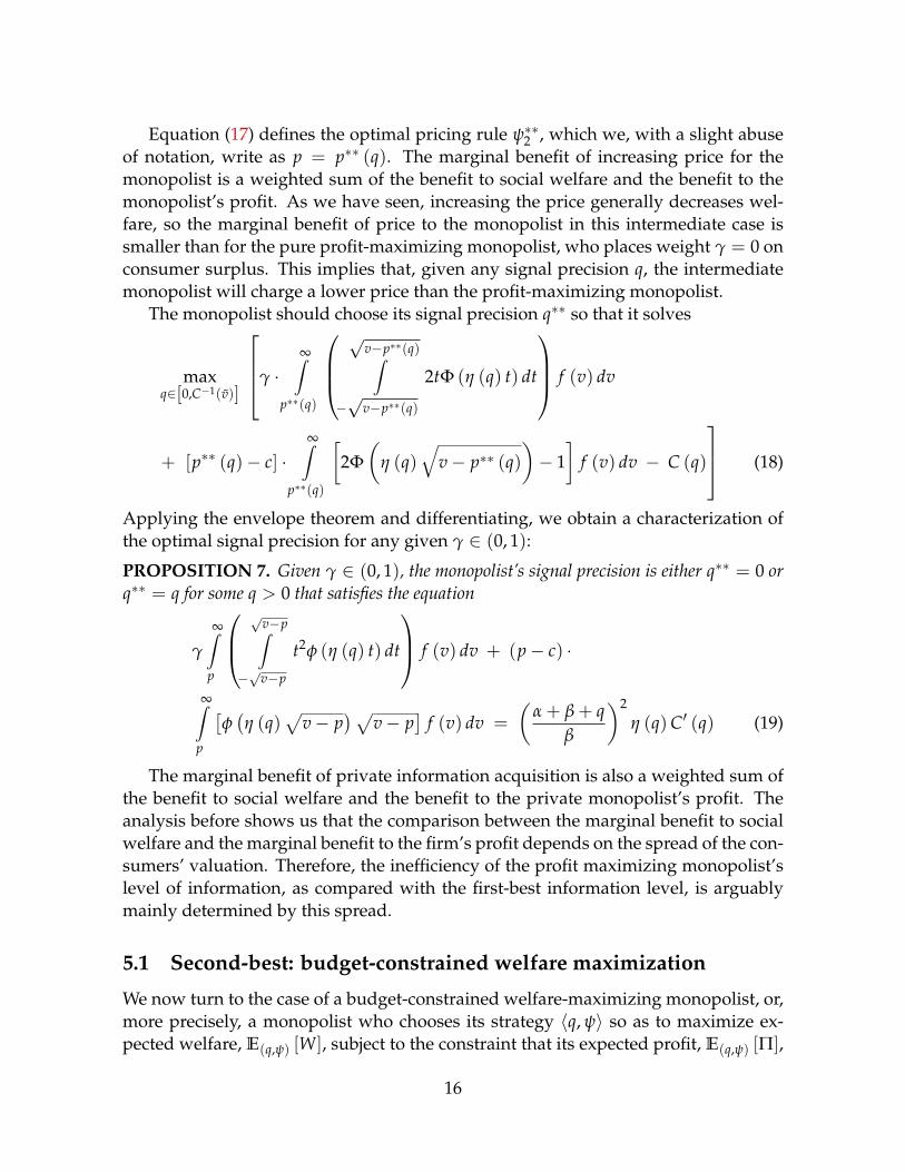
Equation (17) defines the optimal pricing rule ψ∗∗2 , which we, with a slight abuseof notation, write as p = p∗∗ (q). The marginal benefit of increasing price for themonopolist is a weighted sum of the benefit to social welfare and the benefit to themonopolist’s profit. As we have seen, increasing the price generally decreases wel-fare, so the marginal benefit of price to the monopolist in this intermediate case issmaller than for the pure profit-maximizing monopolist, who places weight γ = 0 onconsumer surplus. This implies that, given any signal precision q, the intermediatemonopolist will charge a lower price than the profit-maximizing monopolist.

The monopolist should choose its signal precision q∗∗ so that it solves

maxq∈[0,C−1(v)]

γ ·∞∫

p∗∗(q)

√

v−p∗∗(q)∫−√

v−p∗∗(q)

2tΦ (η (q) t) dt

f (v) dv

+ [p∗∗ (q)− c] ·∞∫

p∗∗(q)

[2Φ(

η (q)√

v− p∗∗ (q))− 1]

f (v) dv − C (q)

(18)

Applying the envelope theorem and differentiating, we obtain a characterization ofthe optimal signal precision for any given γ ∈ (0, 1):

PROPOSITION 7. Given γ ∈ (0, 1), the monopolist’s signal precision is either q∗∗ = 0 orq∗∗ = q for some q > 0 that satisfies the equation

γ

∞∫p

√

v−p∫−√v−p

t2φ (η (q) t) dt

f (v) dv + (p− c) ·

∞∫p

[φ(η (q)

√v− p

)√v− p

]f (v) dv =

(α + β + q

β

)2

η (q)C′ (q) (19)

The marginal benefit of private information acquisition is also a weighted sum ofthe benefit to social welfare and the benefit to the private monopolist’s profit. Theanalysis before shows us that the comparison between the marginal benefit to socialwelfare and the marginal benefit to the firm’s profit depends on the spread of the con-sumers’ valuation. Therefore, the inefficiency of the profit maximizing monopolist’slevel of information, as compared with the first-best information level, is arguablymainly determined by this spread.

5.1 Second-best: budget-constrained welfare maximization

We now turn to the case of a budget-constrained welfare-maximizing monopolist, or,more precisely, a monopolist who chooses its strategy 〈q, ψ〉 so as to maximize ex-pected welfare, E(q,ψ) [W], subject to the constraint that its expected profit, E(q,ψ) [Π],

16

is at least B, where B ≥ 0 is exogenously given. The case B = 0 is of particular in-terest, since it represents a familiar second-best situation, that of a monopolist whostrives to maximize welfare under the requirement that it should cover its costs by itsown revenues.

Let π (0) be the profit obtained by the monopolist in Section 3 (γ = 0), let π (1)be the profit obtained by the monopolist in Section 4 (γ = 1), and for each γ ∈ (0, 1),let π (γ) be the profit obtained by the monopolist in the present section. We thenhave π (0) > 0 > π (1), and π (γ) is continuous in γ for γ ∈ [0, 1]. (The last claimfollows from Berge’s maximum theorem.) Hence, by continuity there exists at leastone γ ∈ (0, 1) for which π (γ) = 0.

PROPOSITION 8. Let γo be such that π (γo) = 0. A monopolist that maximizes E(q,ψ) [W]subject to the budget constraint E(q,ψ) [Π] ≥ 0 will choose the same strategy 〈q∗∗, ψ∗∗〉 asdefined above, for γ = γo, and the budget constraint will be precisely met.

That is to say, we find the budget-constrained monopolist’s behavior by pickingthe parameter value γ so that the budget constraint is exactly met. The intuitionbehind this result is simple: the Lagrangian associated with the budget-constrainedmonopolist’s decision problem can be written as

L (q, ψ, λ) = E(q,ψ) [W] + λE(q,ψ) [Π] ,

where λ ≥ 0 is the Lagrangian multiplier associated with the budget constraint. Bysetting λ = λo = (1− γo) /γo, maximization of L (q, ψ, λo), given λo, is identical withsolving our intermediate monopolist’s problem when γ = γo. And by definition ofthis particular γ-value, E(q,ψ) [Π] = 0, so the budget-constraint is met. To see theintuition why the budget constraint is necessarily precisely met, suppose, by con-tradiction, that the constraint were not binding, so that the monopolist now earns aprofit above B = 0. Then, given its signal precision q∗∗, the monopolist could reduceits price slightly without violating the budget constraint (by continuity), and this wayobtain a slightly higher social welfare, since the latter is monotonically decreasing inthe price, as shown in the proof of Proposition 4.5

6 Numerical simulations

In order to illustrate the above results, we will now consider numerical simulationsresults for the special case of a log-normal value distribution and information coststhat are a positive power of the signal precision. As will be seen, we will be able tonumerically identify the monopolist’s unique signal precision and price, and makecomparative-statics experiments with these.

5Actually for any B less than the profit of the unregulated private monopoly and more than theprofit of public monopoly, there is one γB such that π(γB) = B, the budget constraint will be preciselymet.

17

6.1 Profit maximization

We now turn to our numerical simulations results. Assume that C (q) = bqa forsome b > 0 and a ≥ 1. Furthermore, the consumers’ valuation is assumed to belog-normally distributed with mean v and standard deviation σ.6

Figure 3: Equilibrium price and posterior estimate precision

The first batch of our numerical simulations studies the effect of η (q) on the mo-nopolist’s optimal price (that is, it only studies Equation (9)). Figure 3 shows us thenumerical result when c = 5 and v = 50. The result confirms our conjecture that,depending on the valuation distribution, the effect of η (q) on the monopolist’s op-timal price may be either monotone or non-monotone. When the variance of con-sumers’ valuation distribution is small enough, higher η (q) monotonically increasesthe price; when the variance is large enough, η (q) has a non-monotone effect on theoptimal price. This result is consistent with our reasoning above and the property oflog-normal distribution. With very small σ (such as σ = 5 or σ = 20), the mode of thelog-normal distribution is around v so that a large number of consumers’ valuationis concentrated around v; 7 however, the price is much smaller than v. According toour analysis above, higher η (q) will increase the price. As σ increases, the mode de-

6 In this case, denoted the consumers’ valuation by v, then ln (v) is normally distributed with mean

ln v− ln√

1 + σ2

v2 and variance ln(

1 + σ2

v2

).

7Note that the mode of the log-normal distribution is v exp(− 3

2 ln(1 + σ2/v2)).

18

creases monotonically; when the mode of the distribution is around the price (whenσ = 40), increases in η (q) force the monopolist to decrease the price. When σ islarge enough such that the mode is much smaller than the price, increases in η (q)will firstly force the monopolist to increase the price and then force the monopolist todecrease the price.

The second batch of our numerical simulations is focused on comparative staticswhen consumers’ valuation distribution is given. During the second batch, we as-sume that consumers’ valuation is log-normally distributed with mean v = 50 andstandard deviation σ = 50.

Figures 4a and 4b show the optimal information acquisition and optimal price asfunctions of α when a = 2, b = 0.1, c = 5 and β = 1. Figure 4a shows that a more pre-cise prior for the shared component crowds out the monopolist’s incentive for infor-mation acquisition. Furthermore, with linear information acquisition cost function,when α is small enough, the private information acquisition and α are perfect substi-tutes. Furthermore, the information acquisition decreases in a lower speed than theincrease of α such that the monopolist has a more precise posterior estimate of theconsumers’ ideal products. With our parameter, this decreases the monopolist’s pricein equilibrium, which is consistent with the results from Figure 3.

Figures 5a and 5b show the numerical solutions as functions of β when a = 2,b = 0.1, c = 5 and α = 1. Figure 5a shows that the more concentrated consumers’idiosyncratic ideal product varieties are, the more private information the monop-olist will acquire. The intuition behind the result is that, with more concentratedideal product varieties, private information is more valuable since it helps estimatemore consumers’ ideal products. Therefore, large concentration in consumers’ idealproducts increase the monopolists’ precision of posterior estimate of consumers’ idealproducts; to be consistent with Figure 3, this will decrease the monopolist’s price inequilibrium.

Figures 6a and 6b show the numerical solutions as functions of the power a in thecost function when α = β = 1, c = 5 and b = 0.1. The effect of a on informationacquisition is non-monotone, and is affected by other parameters, especially by thecost parameter b.8 An increase in a reduces the marginal information acquisition costfor signal precision q less than exp

(−1

a

)and increases the marginal information ac-

quisition cost for q greater than exp(−1

a

).9 When both a and b are quite small, the

signal precision in equilibrium is very high; in this case, an increase in a decreases themonopolists information acquisition. As a increases, the information acquisition falls

8An increase in b monotonically increases the marginal cost of information acquisition, and there-fore monotonically decreases the information acquisition in equilibrium.

9To see this, taking derivative of the marginal information acquisition cost with respect to b, wehave bqa−1 (a ln q + 1).

19

(a) Information acquisition

(b) Price

Figure 4: The effect of shared component precision

20

(a) Information acquisition

(b) Price

Figure 5: The effect of idiosyncratic component precision

21

(a) Information acquisition

(b) Price

Figure 6: The effect of a

22

below exp(−1

a

), then the firm has greater incentives to acquire private information

with larger a. Therefore, when b is very small, the increases in a at first decreases η (q)and then increases it; with our parameter setting, this will at first increase the equilib-rium price and then decreases the optimal price. When b is very large, the monopolistacquires very little information. In this case, an increase of the power a increases theequilibrium information acquisition and therefore decreases the equilibrium price.

Figures 7a and 7b show the equilibrium information acquisition and price as func-tions of unit production cost c when α = β = 1 and information acquisition cost func-tion is C (q) = q2/10. From Equation (11), we see that given the price p, an increasein the unit production cost monotonically decreases the marginal benefit of informa-tion acquisition. Therefore, larger unit production cost monotonically decreases theequilibrium information acquisition. Figure 7a confirms this conjecture. Therefore,with a higher unit production cost, the monopolist in equilibrium has a less preciseestimate of individual’s ideal products.

A change of unit production cost has two effects on price: firstly, with our parame-ter setting, decreases in η (q) increase the monopolist’s equilibrium price; secondly, asshown above increases in c imply that the firm incurs less cost by increasing the priceand decreasing the demand. Therefore, higher unit cost increases the equilibriumprice, this is consistent with the results of Figure 7b.

We now turn to our third batch of numerical simulations, in which we study theeffect of a mean-preserving spread of consumers’ valuation distribution. The reasonwhy this may be interesting is that in general a monopolist’s profit, at the monopolyprice, is decreasing in the spread of consumers’ valuation for the good in question.To see this, suppose, first, that all consumers have virtually the same valuation, v ≈50, and that they all have product variety θ = 0 as their ideal, and furthermore theunit production is 0. If the monopolist would know this, he could extract almost allconsumer surplus by setting the price p just below 50 and make profits close to 50.Next, suppose instead that consumer valuations are uniformly distributed betweenzero and one hundred, and that again all consumers’ ideal is the variety θ = 0. Amonopolist would know this and could only extract half the consumer surplus. Hewould again optimally set p close to 50, but now only half the consumers would buy,so his profits would be only 25. Hence, one may ask if this qualitative relationshipholds also in our more general model. If it does, then the monopolist might investless in information acquisition.

To find this out, we now assume that α = β = 1 and C (q) = q2/10, and that con-sumers’ valuation v is log-normally distributed with mean v and variance σ2. For ourpurpose, for each v, we investigate how the change of σ, when keeping v constant,would affect the equilibrium information acquisition and price. Figure 8a shows thatthe qualitative relationship in the above very parsimonious model still holds in ourmore general settings: more dispersion in consumers’ valuation decreases monopo-list’s incentive in private information acquisition.

23

(a) Information acquisition

(b) Price

Figure 7: The effect of unit production cost

24

(a) Information acquisition

(b) Price

Figure 8: The effect of value dispersion

25

Figure 9: Revenue and price given the signal precision

Figure 8b shows the non-monotonic effects of more dispersion in valuation distri-bution on equilibrium price. This figure integrates two effects of more dispersion onthe equilibrium price: the first one is that more dispersion decreases the equilibriuminformation acquisition, and therefore decreases the posterior estimate precision ofindividual’s ideal products; the second one is that by changing the consumer’s valua-tion distribution, the monopolist needs to adjust the price. The first effect on the pricemay be non-monotonic, as we have said in Remark 1, depending on the valuationdistribution. However, the second effect may dominate the first one for the disper-sion effects on price. Figure 9 shows that, given v = 50, η (q) = 1 and c = 5, howoptimal price is adjusted as the standard deviation of consumers’ valuation distribu-tion changes. We can see that, consistent with Figure 8b, the monopolist decreasesthe price when σ is between 0 and around 20 and then increases the price when σ isabove 20.

To see the effects of σ on price shown in Figure 9, we can interpret the adjustmentprocess in terms of Figure 2. When σ is zero, all consumers have valuation v andthe optimal price is shown in Equation (9) by assuming v = v and ignoring the in-tegral. As σ increases, the mode of consumers valuation distribution decreases (seefootnote 6), the shaded area and the rectangle with solid sides in Figure 2 are morevaluable for the monopolist, and the monopolist prefers a lower price. As σ increases,the mode of the valuation distribution is so low that it becomes less valuable to attract

26

(a) (σ, α) (b) (σ, β)

(c) (σ, a) (d) (σ, c)

Figure 10: The effect of (α, β, a, c) on the inefficiencies

27

the consumers with valuation around the mode; the monopolist prefers to increasingthe price to serve only the consumers with high valuation.

6.2 First best

With numerical methods, we can compare the monopolist’s optimal information ac-quisition with the first best. Figure 10 show the difference of the signal precisionswhen consumers’ valuation is log-normally distributed with mean v = 50, and thecost function is C (q) = bqa for b > 0 and a > 1. All parameters are the same as inSection 6.1. The two figures suggest that, although both α and β have some effectson the inefficiencies of the monopoly in acquiring private information, they do notplay a critical role in determining whether the monopolist acquires too much or toolittle private information. Both Figure 10 and Figure 11 show that the dispersion ofconsumers’ valuation distribution determines the inefficiencies of the monopolist’sinformation acquisition. When consumers are homogeneous in their valuation of thegood, the monopolist invests too much in information acquisition. On the contrary,when consumers are very heterogeneous in their valuation, the monopolist has noenough incentive to acquire private information.

Figure 11: The effect of σ on information acquisition

To see why the valuation dispersion affects the inefficiencies of monopolist’s infor-mation acquisition, we can compare the monopolist’s and first-best marginal benefit

28

of information acquisition.Note that the marginal benefit of information acquisition in Equation (15) comes

from attracting more consumers with more precise estimate of individual’s idealproduct. For each valuation v above the unit production cost c, the marginal ben-efit from attracting more consumers by investing in information acquisition is

1η (q)

(β

α + β + q

)2√

v−c∫−√

v−c

t2φ (η (q) t) dt.

Furthermore, by a change of variables, the corresponding first-order condition Equa-tion (11) for the monopolist’s information acquisition can be reformulated as

p− cη (q)

·(

β

α + β + q

)2 ∞∫0

2v2φ (η (q) v) f(

v2 + p)

dv.

This marginal benefit is the marginal benefit from attracting more consumers by in-vesting in information acquisition multiplied by the benefit of selling out one moreunit. From the expression above, we can see that for each valuation v, the marginalbenefit from attracting more consumers by investing in information acquisition is ap-proximately to be

2v2φ [η (q) v]η (q)

·(

β

α + β + q

)2

.

Figure 12 compares the monopoly’s marginal benefit of attracting more consumersby investing in private information with the first-best when α = β = q = 1 andc = 5. It shows that for each v, the first-best marginal benefit of attracting more con-sumers monotonically increases in v, and as v goes to infinity, it goes to β2/[(α + β +q)2η(q)4]. The private monopolist’s marginal benefit of attracting more consumers ismonotonically decreasing in v when v is large enough, and it tends to zero as v goesto infinity. Therefore, there exists one v such that for all v > v, the first-best marginalbenefit is larger than the private monopolist’s, and the discrepancy between thesetwo increases. As σ increases, f (v) increases for high valuation, implying more con-sumers endowed with high valuation. Therefore, the discrepancy between the totalmarginal benefits from attracting more consumers is increasing in σ. Furthermore,in our numerical simulations, p − c is generally much larger than 1; this increasesmonopoly’s marginal benefit of information acquisition. When σ is small, the dis-crepancy between the total marginal benefits from attracting more consumers is notlarge enough to offset the high price in equilibrium; in this case, the monopoly has ahigher marginal benefit of information acquisition. On the contrary, when σ is largeenough, the discrepancy is large enough to offset the effect of high price; in this case,the monopoly has no enough incentive to acquire enough private information.

29

Figure 12: Marginal benefit by attracting consumers

REMARK 2. The numerical results in this subsection are based on the log-normally dis-tributed valuation; however, since the comparison between the marginal benefit of informa-tion acquisition to attract consumers is independent of consumers’ valuation distribution, theresults on the effects of the dispersion of consumers’ valuation on inefficiencies in monopoly’sinformation acquisition are robust to any kind of distribution.

6.3 Second-best

In this subsection we numerically solve for the information acquisition and pricingwhen the goal function is a convex combination of the monopolist’s profit and so-cial welfare. The numerical solutions are shown in Figures 13 and 14; we assume aquadratic information acquisition cost function C (q) = 0.1q2 and c = 5, and that v islog-normally distributed with mean v = 50. We further write κ = − ln (1− γ) andassume that both the variances of shared component and idiosyncratic componentare 1. We will refer to the parameter κ, which is a monotone transformation of the pa-rameter γ, as the welfare weight in the monopolist’s goal function. We will analyzethe case when κ ∈ {10, 20, 40} so that we can see how the changes in the weight affectthe equilibrium pricing and information acquisition..

Figure 13 shows that the monopolist caring about both profit and welfare prefersa price between the private monopolist’s optimal price and the first-best price. When

30

Figure 13: Price as a function of valuation distribution, for different welfare weights

γ is close to 1, the price is close to the first-best price; on the contrary, when γ is notlarge enough, the price is close to private monopolist’s optimal price; more specif-ically, the monopolist’s optimal price is monotonically increasing in the weight γ.Furthermore, since the profit-maximizing monopolist’s optimal price may be non-monotonic in the valuation dispersion, and the marginal benefit of the monopolistcaring both welfare and profit is a weighted sum of the marginal benefit to privatemonopoly and marginal benefit to social welfare, the optimal price for the monopolistcaring both social welfare and profit and specifically the second-best price, depend-ing on the weight γ and other parameters, may also be non-monotonic in valuationdispersion.

Figure 14 illustrates the relationship between information acquisition and valua-tion dispersion σ for different values of κ. When κ is large enough, the monopolistput more weight on social welfare and the information acquisition in equilibrium ismore close to the first-best information acquisition; on the contrary, when κ is verysmall, the monopolist behaves more like the private monopolist in information ac-quisition. Furthermore, although both the private monopolist’s and and first-bestinformation acquisition are monotonic in consumers’ valuation dispersion, the infor-mation acquisition of the monopolist caring both the profit and social welfare maybe non-monotonic in the dispersion. Specifically, Figure 14 shows that when κ is notlarge enough, the monopolist’s information acquisition is increasing in the dispersion

31

Figure 14: Information acquisition as a function of valuation distribution, for differentwelfare weights

when the dispersion is not large enough, and, contrarily, when the dispersion is largeenough, the monopolist’s information acquisition is decreasing in the dispersion.

One final comment is that, although the marginal benefit of information acquisi-tion for the monopolist is a weighted sum of the marginal benefit to the profit andthe marginal benefit to the social welfare, the optimal information acquisition of themonopolist who cares both the profits and social welfare may be higher than both theprivate monopolist’s and first-best information acquisition. This happens when theweight is not large enough and consumers’ valuation dispersion is intermediate. Theintuition of this result is that, when the dispersion σ is relatively large, the marginalbenefit from attracting more consumers is larger than the private monopolist; at thesame time, the price of the monopolist is much higher than the first-best: In thiscase, the marginal benefit of information acquisition is higher than both the marginalbenefit of the private monopolist and the first-best marginal benefit, resulting in aninformation acquisition which is higher than both private monopolist’s optimal in-formation acquisition and the first-best information acquisition. Furthermore, whenthe dispersion is quite small, the dispersion is not large enough to generate a highmarginal benefit to the social welfare by attracting more consumers to offset the ef-fect of the high price; in this case, the monopolist caring both the profits and socialwelfare acquires less information than the private monopolist and more information

32

than the first-best. On the contrary, when the dispersion is large enough, the marginalbenefit to the social welfare from attracting more consumers is large enough to offsetthe effect of high price; in this case, the monopolist caring both the profits and socialwelfare acquires more information than the private monopolist and less informationthan the first-best.

7 Extensions

Our model is very simple and based on heroic assumptions. We here briefly discussa few directions in which the model may be generalized; the dimensionality of prod-uct variety, multiplicity of product variety and oligopolist competition. For while themonopolist in our model only supplies one variety and the space of varieties is one-dimensional, in practice monopolists usually provide a whole menu of product vari-eties where each variety has many attributes and hence is multi-dimensional. More-over, while competition is absent from our model, in practice there is competition orat least the threat of potential entrants. While an analysis of the mentioned generalcases appears quite a challenge and falls outside the scope of the present study, wehere briefly sketch how the present model can be generalized.

First, in order to capture multiplicity and multi-dimensionality of varieties, themost natural generalization is arguably to let the monopolist choose a finite menuM = {(x1, p1) , ..., (xm, pm)} of product varieties and prices for these but maintain thehypothesis of unit demand. In such a setting each consumer chooses which variety,if any, to buy. Let thus each variety xi be a vector in X = Rk for some positive integerk, the dimensionality of varieties, and assume a fixed cost d (xi) > 0 associated witheach variety, alongside its unit cost c (xi) > 0 of production (where costs thus maydepend on the variety). The monopolist’s decision problem then is to choose a menuM from among the setM = ∪m∈N (X×R+)

m of all finite menus, or, in other words,how many and what varieties, and what price for each variety. Given a goal func-tion of the sort analyzed in the preceding sections, this is a challenging optimizationproblem. However, given such a menu M = {(x1, p1) , ..., (xm, pm)}, offered by themonopolist, each consumer’s choice is simple, namely, to either buy no unit or to buyone unit of the variety that gives most utility. To be more specific, let a consumer typebe a pair τ = (θ, v) ∈ X ×R+ and let the utility for a consumer of type τ = (θ, v)from purchasing any variety xi at any price pi be defined as in Section 2;

ui = v− pi − ‖θ − xi‖2 ,

and letuτ (M) = max {u1, ..., um} .

Thus uτ (M) is the utility a consumer of type τ = (θ, v) obtains from any menu M of-fered by the monopolist. The consumer will buy a unit if and only if uτ (M) ≥ 0. Like

33

in Section 2, one may, for analytical tractability, treat θ and v as statistically indepen-dent random variables, each with an absolutely continuous probability distribution.If θ is multi-variate normal and the monopolists signal is additive with normally dis-tributed noise, and if the fixed and marginal costs are the same for all varieties, thenmuch of the preceding machinery applies, although with substantial mathematicalchallenge. However, for any given fixed production cost, d (assumed to be the samefor all varieties), an upper bound on the number m of varieties is m+ = v/d. In orderto solve (at least numerically) the monopolist’s decision problem, one may then pro-ceed by solving it first for each m = 1, 2, .., m+, and thereafter choose the right num-ber, m∗∗ ∈ {0, 1, ..., m+} of varieties. Moreover, at least in the case of one-dimensionalvarieties (k = 1), the following heuristic could be explored. For m = 1 solve as inSections 3 to 5 above, that is, choose variety x∗∗. For m = 2, place instead the two va-rieties at equal distance from x∗∗, and optimize over this distance. For m = 3, choosevariety 1 to be x∗∗ and place varieties 2 and 3 on each side of 1, at equal distance fromx∗∗, and optimize over this distance etc.

Second, an analytically more tractable model extension that allows for multiple,but one-dimensional, varieties would be to let the monopolist select a whole "productline segment" L = [xo − t, xo + t] as in Mussa and Rosen (1978), and require it tocharge a uniform price p for all varieties in this line segment L. In this case, it is easilyverified that the monopolist’s optimal location of the product line segment is to centerit on x∗∗, that is, to pick xo = qs/ (α + q). This follows from the analysis above of thespecial case t = 0 in combination with the observation that now the demand functiongeneralizes to

D (x, p, t) =∞∫

p

Pr[x− t−

√v− p ≤ θ ≤ x + t +

√v− p

]f (v) dv

The optimality of the choice xo = qs/ (α + q) holds when the width t ≥ 0 ofthe product line segment is exogenous. Suppose the width is endogenous and if themonopolist does not only have a constant unit cost c ≥ 0 of production but also anincreasing cost e (t) associated with the width t ≥ 0 of its product line, then t canbe determined by a first-order condition equating the marginal cost of t, e′ (t), to itsmarginal benefit to the monopolist (see the models in Mussa and Rosen (1978) andSpence (1975)). As shown in Spence (1976a,b), this choice of t will typically be sociallyinefficiency when the monopolist’s information about consumer preferences is fixed.An interesting avenue for further research is thus to explore this potential inefficiencyin the case of endogenous information.

Third, a few words about oligopolistic competition. An extension in such a direc-tion would be extremely interesting. The fundamental underlying question is thenthe effect of competition on producers’ incentives to find out about consumer pref-erences? More precisely, suppose now that there are two profit-maximizing firms,

34

each modelled along the lines of the profit-maximizing monopolist in Section 3, andthat each firm first has to choose its signal precision, then its product variety andprice. A number of alternative scenarios are possible here. Arguably, the most ba-sic and canonical scenario is that of simultaneous-move duopoly, that is, two firmswho simultaneously first choose their signal precisions, keep their signal precisionsand signal realizations as their private information, and then simultaneously choosetheir own product variety and price. What can then be said? A conjecture for sym-metric Nash equilibrium is that they will each choose the same signal precision,q1 = q2 = q∗, that they will choose their own product variety as under monopoly,that is x∗1 = q∗s1/ (α + q∗) and x∗2 = q∗s2/ (α + q∗), and that they will choose thesame price, p∗1 = p∗2 = p. If so, what is then q∗ and p∗, and how do these relate for theprofit-maximizing monopolist’s choice and to the first-best monopoly choice? And isthe conjecture at all true? To explore these questions appears as a natural next step inthis exploration of producers’ endogenous information about consumer preferences.

8 Conclusion

This paper examines a monopolist’s production variety choice, price setting and in-formation acquisition. In our model the marginal cost of production of the goodis constant, and the monopoly will choose the efficient variety. Compared with first-best, the profit-maximizing monopoly sets too high a price. However, the inefficiencyin private monopoly’s information acquisition depends on the parameters, especiallyon the consumer’s valuation distribution. With log-normally distributed valuation,our numerical results show that there is a critical point of the spread such that the pri-vate monopoly acquires too much information when the spread is smaller than thecritical point and the opposite is true when the spread is larger than the critical point.Compared with the second-best price setting and the information acquisition wherethe monopoly’s profit is constrained, the profit-maximizing monopoly will generallyset too high a price, and the inefficiency in the information acquisition is still deter-mined by the consumers’ valuation spread.

The results in the paper are still not as general as we would wish, and some ofthem rely on the numerical method. More general results on the monopoly’s choiceunder consumers’ preference uncertainty need further investigation. For instance,while we here focus the entire analysis on endogenous information about consumerpreferences over product varieties, a relevant consideration is that of endogenous in-formation about consumers’ valuations of their ideal product variety. There are otherimportant factors that may affect the value of monopoly’s private information. Forinstance, the threat and competition from the potential entrant may also affect themonopoly’s information acquisition choice (see Dimitrova and Schlee, 2003). To in-corporate these factors into the model studying monopoly’s information acquisition

35

would be very interesting.

References

Armstrong, M. and D. E. Sappington (2007). Recent developments in the theory ofregulation. Handbook of industrial organization 3, 1557–1700.

Bester, H. (1993). Bargaining versus price competition in markets with quality uncer-tainty. American Economic Review 83(1), 278–288.

Bester, H. and K. Ritzberger (2001). Strategic pricing, signalling, and costly informa-tion acquisition. International Journal of Industrial Organization 19(9), 1347–1361.

Boiteux, M. (1971). On the management of public monopolies subject to budgetaryconstraints. Journal of Economic Theory 3(3), 219–240.

Casado-Izaga, F. J. (2000). Location decisions: the role of uncertainty about consumertastes. Journal of Economics 71(1), 31–46.

Dimitrova, M. and E. E. Schlee (2003). Monopoly, competition and information ac-quisition. International Journal of Industrial Organization 21(10), 1623–1642.

Harter, J. F. (1997). Hotelling’s competition with demand location uncertainty. Inter-national Journal of Industrial Organization 15(3), 327–334.

Król, M. (2012). Product differentiation decisions under ambiguous consumer de-mand and pessimistic expectations. International Journal of Industrial Organiza-tion 30(6), 593–604.

Meagher, K. J. (1996). Managing change and the success of niche products. Technicalreport.

Meagher, K. J. and K. G. Zauner (2004). Product differentiation and location decisionsunder demand uncertainty. Journal of Economic Theory 117(2), 201–216.

Meagher, K. J. and K. G. Zauner (2005). Location-then-price competition with uncer-tain consumer tastes. Economic Theory 25(4), 799–818.

Meagher, K. J. and K. G. Zauner (2011). Uncertain spatial demand and price flexibil-ity: A state space approach to duopoly. Economics Letters 113(1), 26–28.

Mussa, M. and S. Rosen (1978). Monopoly and product quality. Journal of Economictheory 18(2), 301–317.

36

Ramsey, F. P. (1927). A contribution to the theory of taxation. Economic Journal 37(145),47–61.

Spence, A. M. (1975). Monopoly, quality, and regulation. The Bell Journal of Eco-nomics 6(2), 417–429.

Spence, M. (1976a). Product differentiation and welfare. American Economic Re-view 66(2), 407–414.

Spence, M. (1976b). Product selection, fixed costs, and monopolistic competition.Review of Economic Studies 43(2), 217–235.

Vives, X. (1984). Duopoly information equilibrium: Cournot and Bertrand. Journal ofEconomic Theory 34(1), 71–94.

37