j ourna l homepage: www.e lsev ie r .com/ locate /enggeo
Probabilistic and spatial assessment of liquefaction-induced settlementsthrough multiscale random field models
Qiushi Chen a, Chaofeng Wang a, C. Hsein Juang b,a,⁎a Glenn Department of Civil Engineering, Clemson University, Clemson, SC 29634, USAb College of Transportation Engineering, Tongji University, Shanghai 200092, China
⁎ Corresponding author at: Glenn Department of Civil EClemson, SC 29634, USA.
Article history:Received 7 March 2016Received in revised form 1 July 2016Accepted 4 July 2016Available online xxxx
Evaluation of liquefaction-induced settlements over an extended area requires the integration of different solu-tion models that can account for the liquefaction resistance of a given soil profile and its spatial dependenceacross scales. In this paper, a CPT-based liquefaction model is adopted to estimate the liquefaction-induced set-tlement at individual sounding locations. The model is then integrated with multiscale random field models toaccount for spatial variability of soil properties. One important advantage of the proposed framework is its abilityto consistently refine and provide settlement estimations across different scales, from regional and geologic unitscales down to a local, site-specific scale. The proposed methodology is then applied to the AlamedaCounty, California, an earthquake-prone region, to illustrate the procedure for probabilistic and spatial assess-ment of liquefaction-induced settlements at different scales.
Keywords:Liquefaction settlementCone penetration test (CPT)Spatial variabilityProbabilistic analysisRandom field model
1. Introduction
Assessment and mitigation of regional liquefaction hazard require areliable tool for evaluating not only theprobability of liquefaction occur-rence, but also, more importantly, the associated effects within a region.Ground surface settlements due to soil liquefaction have been one of themajor causes for infrastructure damages during an earthquake. Evalua-tion of liquefaction-induced settlement at individual locations, wherefield tests such as the cone penetration test (CPT) are performed, canbe achieved through classical empirical liquefactionmodels. Tomap liq-uefaction settlement over an extended area, however, the spatial de-pendence of soil properties across the region must be taken intoaccount. This paper presents a framework for integrating the classicalliquefaction models (e.g., a CPT-based liquefaction-induced settlementmodel) and tools from geostatistics (e.g., multiscale random fieldmodels) for the probabilistic and spatial assessment of liquefaction-in-duced settlements across an earthquake-prone region, from regionaland geologic unit scales down to a local, site-specific scale.
1.1. Previous work
Evaluation and prediction of liquefaction-induced settlement havebeen the subject of intensive research for the past several decades.Among various approaches, use of empirical relationships based on
ngineering, Clemson University,
the correlation of observed soil behavior with various in-situ indextests or laboratory tests remains the dominant approach for assessingliquefaction-induced settlement, e.g., (Lee and Albaisa, 1974;Tokimatsu and Seed, 1984, 1987; Nagase and Ishihara, 1988; Ishiharaand Yoshimine, 1992; Pradel, 1998; Shamoto et al., 1998; Zhang et al.,2002; Wu and Seed, 2004; Tsukamoto et al., 2004; Lee, 2007; Cetin etal., 2009a, 2009b; Lu et al., 2009; Ueng et al., 2010; Tsukamoto andIshihara, 2010; Juang et al., 2013; Valverde-Palacios et al., 2014). In par-ticular, using cone penetration test (CPT) data, Zhang et al. (2002) pro-posed amethod that couples the volumetric strain chart by Ishihara andYoshimine (1992) to the classical CPT-based liquefaction model byRobertson andWride (1998) for evaluation of liquefaction-induced set-tlements. Building on the work of Zhang et al. (2002) and Juang et al.(2013) proposed a probabilistic approach to estimate probability of ex-ceeding a settlement threshold. Using laboratory data and empiricalcorrelations, probabilistic models were developed in Cetin et al.(2009a,b) for cyclic volumetric and shear strains, whichwere correlatedto typical field index test results such as the corrected standard penetra-tion test blow counts or the cone penetration test tip resistance, to pre-dict field settlements.
All of the aforementioned work estimates the liquefaction-inducedsettlement, or the probability of exceeding a particular settlementthreshold, at individual locations. To assess the consequences of lique-faction over extended areas or tomap the estimated liquefaction settle-ments to a region, it is necessary to account for the spatial dependenceof soil properties and/or the predicted settlements. Tools developed ingeostatistics have received considerable attention in recent years andhave been applied to assess liquefaction hazard over large regions. For
instance, Liu and Chen (2006) used CPT measurements to estimate thespatial structure of soil deposits. Then, random field models werecoupled with Monte Carlo simulations to assess liquefaction potentialin the Yuanlin area of Taiwan. Vivek and Raychowdhury (2014) explic-itly considered the spatial variations of soil indices from CPT soundingswhen evaluating liquefaction potential. It has been found that the prob-ability of liquefaction could be significantly underestimated if the spatialdependence of soil indices has not been considered. Chen et al. (2015)developed a random field-based approach to map liquefaction poten-tials across scales, where the spatial variability of the Liquefaction Po-tential Index (LPI) developed by Iwasaki et al. (1978, 1982)) isexplicitly considered through internally-consistent probabilistic modelsdeveloped at multiple scales. LPI has also been adopted andmodified toassess liquefaction potentials at individual CPT soundings or over ex-tended region (Sonmez, 2003; Sonmez and Gokceoglu, 2005;Papathanassiou et al., 2005; Holzer et al., 2006; Baise et al., 2006; Lenzand Baise, 2007; Thompson et al., 2007; Juang et al., 2008b). In anotherrecent work by van Ballegooy et al. (2015), four liquefaction vulnerabil-ity parameters, including the LPI, were used tomap liquefaction hazardsin the Christchurch area using an extensive CPT database. In contrast tothe substantial efforts incorporating geostatistics tools into liquefactionpotential evaluation, relatively few studies have addressed liquefaction-induced settlement over an extended area. In Hinckley (2010) andBartlett et al. (2007), the classical methods of Tokimatsu and Seed(1987), Ishihara and Yoshimine (1992), Bartlett and Youd (1995),Youd et al. (2002) and Yoshimine et al. (2006) are employed to calculateliquefaction-induced lateral spread and ground settlement, which areplotted within their respective surficial geologic units. Each geologicunit is then assigned an estimate of grounddeformation based on statis-tical analysis.
In this work, a CPT-based liquefaction model is coupled with novelgeostatistics tools for the probabilistic and spatial assessment of the liq-uefaction-induced settlements over a region and across different scales.The remainder of the paper is structured as follows: in Section 2, theclassical Robertson and Wride 1998 CPT-based liquefaction model isbriefly presented, which will be used to evaluate the liquefaction-in-duced settlement in Section 3. In Section 4, multiscale random fieldmodels are developed to map the liquefaction settlement over the re-gion of interest. The proposed framework is then applied to analyze liq-uefaction settlement hazards in an earthquake-prone region, i.e., theAlameda County of California, in Section 5 followed by some concludingremarks in Section 6.
2. The updated Robertson and Wride 1998 CPT-based liquefactionmodel
The CPT-based liquefaction model proposed by Robertson andWride (1998) and subsequently updated by Robertson (2009) isadopted in this work to evaluate the liquefaction resistance of sandysoils. The main elements of this classical procedure are briefly summa-rized in this section. The evaluation involves the use of two variables:the capacity of the soil to resist liquefaction, expressed in terms of thecyclic resistance ratio (CRR); and the seismic demand on a soil layerplaced by a given earthquake, expressed in terms of the cyclic stressratio (CSR). If the estimated CSR is greater than CRR, the soil is said toliquefy during the given earthquake.
The cyclic resistance ratio (CRR) is estimated as
CRR ¼ 0:8333 qc1Nð Þcs=1000� �þ 0:05 if qc1Nð Þcsb50
93 qc1Nð Þcs=1000� �3 þ 0:08 if 50≤ qc1Nð Þcsb160
ð1Þ
The equivalent clean sand normalized penetraction resistance, de-noted as (qc1N)cs, is given as
qc1Nð Þcs ¼ Kc qc1Nð Þ ð2Þ
where the conversion factor Kc for grain characteristics is calculatedfrom the soil behavior type index Ic as
Kc ¼ 1 for Ic ≤1:64−0:403I4c þ 5:581I3c−21:63I2c þ 33:75Ic−17:88 for IcN1:64
�ð3Þ
and qc1N is the normalized cone penetration resistance calculated as
qc1N ¼ qc−σvo
Pat
� �Pat
σ 0vo
� �n
ð4Þ
where Pat = 1 atm of pressure (100 kPa); Pat/σvo' should not exceed a
value of 1.7 as specified by Youd et al. (2001); qc is the measured conepenetration resistance; n is the stress exponent, given by
n ¼ 0:381 Icð Þ þ 0:05σ 0
vo
Pat
� �−0:15 where n≤1: ð5Þ
The soil behavior type index, Ic, is defined by Robertson and Wride(1998) as
Ic ¼ffiffiffiffiffiffiffiffiffiffiffiffiffiffiffiffiffiffiffiffiffiffiffiffiffiffiffiffiffiffiffiffiffiffiffiffiffiffiffiffiffiffiffiffiffiffiffiffiffiffiffiffiffiffiffiffiffiffiffiffiffiffiffiffiffiffiffiffiffi3:47− logQð Þ2 þ 1:22þ logFð Þ2
qð6Þ
where Q and F are the normalized tip resistance and friction ratio, re-spectively.
Q ¼ qc−σvo
σ 0vo
� �ð7Þ
F ¼ f sqc−σvo
� �� 100% ð8Þ
For the cyclic stress ratio (CSR), the following adjusted form is used
CSR ¼ 0:65amax
g
� �σvo
σ 0vo
� �rdð Þ 1
MSF
� �1Kσ
� �ð9Þ
where amax is the peak horizontal acceleration at the ground surfacegenerated by a given earthquake; g is the gravitational acceleration;σvo and σvo
' are the total and effective vertical overburden stresses, re-spectively; rd is the depth-dependent shear stress reduction coefficient;MSF is themagnitude scaling factor;Kσ is the overburden correction fac-tor for the cyclic stress ratio (Kσ=1 forσvo
' b 1 atm (1 atm=100 kPa)).The stress reduction factor, rd, is estimated based on the recommenda-tion by Youd et al. (2001), which takes the following form
The magnitude scaling factor MSF also follows the recommendationin Youd et al. (2001) as
MSF ¼ 102:24
M2:56w
ð11Þ
where Mw is the moment magnitude of the earthquake.Once CSR and CRR are obtained, the factor of safety against liquefac-
tion can be derived
FS ¼ CRRCSR
: ð12Þ
The above classical liquefactionmodel expresses the liquefaction po-tential of a given soil profile in terms of factor of safety. For cases wherethere is a need to express the liquefaction potential in terms of liquefac-tion probability, a probabilistic version of the Robertson and Wride
137Q. Chen et al. / Engineering Geology 211 (2016) 135–149
method is developed by Ku et al. (2012) that links the factor of safety(FS) to the liquefaction probability (PL), expressed as
PL ¼ 1−Φ0:102þ ln FSð Þ
0:276
� �≈
1
1þ FS=0:9ð Þ6" #
ð13Þ
where Φ is the standard normal cumulative distribution function. Itshould be noted that the above relation is specific to the Robertson
and Wride (1998) model; therefore, the factor of safety (FS) must becomputed using the Robertson and Wride method. Also, coefficients inthe above relation are calibrated against the compiled liquefaction data-base in Ku et al. (2012) with the assumption that the modeling error ofthe factor of safety follows a lognormal cumulative distribution functionwith a constant coefficient of variation.
3. Probabilistic estimation of liquefaction-induced settlement at individual CPT sounding
Building on the classical CPT-based liquefactionmodel, the liquefaction-induced settlement is approximated as a summation of the product of thevolumetric strain in each soil layer that is susceptible to liquefaction and the corresponding layer thickness. For a site with level ground that is farfrom any freewater surface, such an approximation is reasonable since the volumetric strain is approximately equal to the vertical strain.When slop-ing or nearly free-faced ground is involved in the analysis, the deviatoric- or shearing-induced deformation should be considered when estimatingground settlement. For instance, Wu and Seed (2004) recommended increasing the ground settlement estimation by an amount equal to 10–20% ofthe observed or estimated lateral ground displacement. If the estimated lateral ground displacement is smaller than 0.3 m, the influence of thedeviatoric deformation is insignificant. In this study, we assume the level ground condition for our evaluation, where the predicted liquefaction-in-duced settlement S is estimated as Juang et al. (2013)
S ¼Xni¼1
εviΔziINDi ð14Þ
where εvi is the volumetric strain of the ith layer;Δzi is the thickness of the ith layer; INDi is an indicator of liquefaction occurrence in the ith layer; andn is the total number of layers. In Zhang et al. (2002), IND is taken as 1 for all soil layers. It should be noted that, the adopted Zhang et al. (2002)modelhas been previously critically evaluated in the literature. For instance, Juang et al. (2013) found that the Zhang et al. (2002) model tends to overes-timate the post-liquefaction settlement. A bias factor for the Zhang et al. (2002)model may be calibrated given a compiled liquefaction-induced set-tlement database to correct the model prediction, as suggested by Juang et al. (2013).
For sand-like soils, the volumetric strain εvi of the ith layer is a function of the factor of safety of the ith layer, denoted as FSi, and the clean-sandequivalence of the corrected cone tip resistance, denoted as qi. Following the previouswork of Zhang et al. (2002) and Juang et al. (2013) that coupledthe CPT-based method (Robertson and Wride, 1998) with the volumetric strain relationship (Ishihara and Yoshimine, 1992), the volumetric straincan be approximated with the following equation
Fig. 1 plots the relation given in Eq. (15) along with the design chart by Ishihara and Yoshimine (1992), where q is the clean-sand equivalence ofthe corrected cone tip resistance.
It is noted that, in a deterministic analysis, the indicator function INDi in Eq. (14) is equal to 0 if the ith layer does not liquefy and equal to 1 if theith layer liquefies. In the case of a probabilistic analysis, INDimay be treated as a random variable with its expected value E[INDi] and variance V[INDi]related to the probability of liquefaction PLi of the ith layer (Juang et al., 2013). Accounting for model uncertainties, the FS and q in Eq. (15) are nowboth nominal values calculated from the measurement, not the actual value. As shown by Juang et al. (2013), the nominal values can be estimatedfrom the probability of liquefaction as
E INDi½ � ¼ PLi ð16Þ
V INDi½ � ¼ PLi 1−PLi
� �: ð17Þ
The liquefaction probability PLi of the ith layer may be determined using a PL−FS mapping function previously proposed by Ku et al. (2012) asdefined in Eq. (13). Then, the probabilistic version of the predicted liquefaction settlement, S, at an individual CPT sounding is characterized by itsmean value μS and variance σS
2 as (Juang et al., 2013)
μS ¼Xni¼1
εviziPLi∂ ð18Þ
Fig. 1. Chart for estimating the post-liquefaction volumetric strain of clean sand. Adopted from Juang et al. (2013) and Zhang et al. (2002) with the original source data from Ishihara andYoshimine (1992). Units for the clean-sand equivalence of the corrected cone tip resistance, q, is in kg/cm 2(≈100 kPa).
A further development of the above probabilistic settlement model allows the incorporation and quantification of model error. As suggested byJuang et al. (2013), a multiplicative model bias factorM is introduced and the corrected settlement prediction, denoted as Sa, for a future case can beexpressed as
Sa ¼ MS ¼ MXni¼1
εviziINDi: ð20Þ
Assuming that M is independent of S, the mean and variance of the corrected settlement are then given as (Juang et al., 2013)
μa ¼ μMμS ð21Þ
σ2a ¼ μ2
Mσ2S þ σ2
Mμ2S þ σ2
Mσ2S ð22Þ
where μM andσM are themean and standard deviation ofM; μS andσS are themean and standard deviation of the predicted settlement S as defined inEqs. (18) and (19), respectively. The mean and standard deviation of the model bias factor M may be derived empirically from a database of lique-faction case histories.
4. Characterization of spatial dependence through random fieldmodels
The procedure described in Sections 2 and 3 estimates the settle-ment, either as the nominal value, as in Eq. (20), or as an random vari-able with mean and variance given in Eqs. (21) and (22). Suchestimation is performed at individual CPT sounding locations. To assessthe spatial extent of liquefaction damage across a region where the set-tlement estimations at each location vary, spatial dependence must beconsidered. In this section, geostatistical tools and multiscale randomfield models (Baker et al., 2011; Chen et al., 2012, 2015) will be usedto characterize spatial dependence and to simulate settlement exceed-ance at unsampled locations.
4.1. Semivariogram for characterization of spatial dependence
In this study, spatial dependence is described using a form of covari-ance known as the semivariogram, γ(h), which is equal to half the var-iance of two random variables separated by a vector distance h
γ hð Þ ¼ 12Var Z uð Þ−Z uþ hð Þ½ � ð23Þ
where Z(u) is the variable under consideration as a function of spatiallocation u; Z(u + h) is the lagged version of the variable. Sometimes,Z(u) is referred as the “tail” variable; Z(u + h) is referred as the“head” variable in the geostatistics literature. Under the condition ofsecond-order stationarity (spatially constant mean and variance), thesemivariogram is related to other commonly usedmeasures to quantifyspatial correlation, i.e., the covariance COV(h) and the correlation ρ(h),as
γ hð Þ ¼ COV 0ð Þ−COV hð Þ ð24Þ
γ hð Þ ¼ COV 0ð Þ 1−ρ hð Þ½ � ð25Þ
where COV(0) is the covariance at h = 0 and equals to the varianceσ2. The semivariogram γ(h) is typically preferred by geostatisticscommunity because it only requires the increment Z(u) −Z(u+ h) to be second-order stationary, i.e., the intrinsic hypothesis,which is a weaker requirement than the second-order stationarity ofthe variable itself.
It is possible to define a vector h to account for both separation dis-tance and orientation. The most common approach to modeling the
139Q. Chen et al. / Engineering Geology 211 (2016) 135–149
geometric anisotropy is to define a scalar distance measure as (Isaaksand Srivastava, 1989)
h ¼ffiffiffiffiffiffiffiffiffiffiffiffiffiffiffiffiffiffiffiffiffiffiffiffiffiffiffiffiffiffiffiffiffiffiffiffiffiffiffiffiffiffiffiffiffiffiffiffiffiffiffiffiffiffihxax
� �2
þ hyay
� �2
þ hzaz
� �2s
ð26Þ
where hx, hy and hz are the scalar component of the vector h along thefield's principal axes; scalar quantities ax, ay and az are ranges that spec-ify how quickly spatial dependence decreases along those axes. Charac-terization and inference of spatial dependence remains a challengingand, to some extent, controversial task. Specific forms of spatial struc-ture adopted in this study will be discussed in more detail in the exam-ple application section.
The definition of semivariogram presented above is written in theform of original values of the variables of interest. As pointed out byGringarten and Deutsch (2001), it is rare inmodern geostatistics to con-sider the untransformed data. The commonly adopted Gaussian simula-tion technique requires a prior Gaussian transformation of the data. Tothis end, the inference of the variogram model will be performed onthe transformed data, which are obtained by the normal score mappingtechnique (Goovaerts, 1997). Chen et al. (2012) showed that suchtransformation does not adversely affect the prescribed spatial struc-ture. Nevertheless, the validity of the correlation should be verified toensure that the desired spatial dependence relationship is upheld afterthe transformation.
4.2. Spatial correlation across scales
The previously described spatial correlation has been extended toaccount for the multiscale nature of soil variability (Chen et al., 2012).This extension allows a higher resolution random field to be adaptivelygenerated around areas of high interest, such as adjacent to critical in-frastructures, or around areas of abundant field data. The key of thismultiscale extension is to consistently represent fine and coarse scalerandom fields while maintaining appropriate spatial correlation struc-tures across scales.
In this work, two scales of interest are considered and all subsequentdevelopment applies to variables following the standard Gaussian dis-tribution, i.e., variables after a normal score transformation. The deriva-tion of spatial correlation across scales is based on the notion thatmaterial properties at the coarser scales are the arithmetically averagedvalues of the properties over corresponding areas at the finer scales
ZcI ¼
1N
XNi¼1
Z fi Ið Þ ð27Þ
where superscripts ‘c’ and ‘f’ correspond to coarse and fine scales, re-spectively; N = number of fine scale points within a coarse scale area(element) I. Defining the variable of interest at the fine scale and usingsuch a relation, the expression for the variances and spatial correlationsof coarse scale variables of interest can be explicitly derived.
The mean of a coarse scale element ZIc can be derived by taking theexpectation of Eq. (27) as
μZc ¼ E ZcI
� � ¼ 1N
XNi¼1
μZ fi Ið Þ
¼ 0 ð28Þ
where μZi(I)f is the mean at the fine scale, which is equal to zero for vari-ables following the standard Gaussian distribution. Accordingly, if thevariance of the fine scale variable is unity, the coarse scale variancecan be computed as
σ2Zc ¼ E Zc
I
� �2h i−0 ¼ 1
N2
XNi¼1
XNj¼1
ρZ fi ;Z
fjσZ f
iσZ f
j: ð29Þ
The covariance between any two elements Zi and Zj within the ran-dom field is defined as
COV Zi; Z j� � ¼ ρZi ;Z j
σZiσZ j : ð30Þ
The correlations between all considered scales can be calculated byrearranging the definition of covariance such that
ρZi ;Z j¼ COV Zi; Z j
� �σZiσZ j
ð31Þ
where Zi and Zj are two elements within the random field at any scalewith variance σZi
2 and σZj2. By making appropriate substitutions at
each scale using Eqs. (30) and (31), the correlation between elementsat different scales can be defined as
ρZcI ;ZcII¼
XN
i¼1
XN
k¼1ρZ f
i Ið Þ ;Zfk IIð ÞffiffiffiffiffiffiffiffiffiffiffiffiffiffiffiffiffiffiffiffiffiffiffiffiffiffiffiffiffiffiffiffiffiffiffiffiffiffiffiffiffiffiXN
i¼1
XN
j¼1ρZ f
i Ið Þ ;Zfj Ið Þ
r ffiffiffiffiffiffiffiffiffiffiffiffiffiffiffiffiffiffiffiffiffiffiffiffiffiffiffiffiffiffiffiffiffiffiffiffiffiffiffiffiffiffiffiXN
i¼1
XN
j¼1ρZ f
i IIð Þ ;Zfj IIð Þ
r ð32Þ
ρZ f ;ZcI¼
XN
i¼1ρZ f ;Z f
i Ið ÞffiffiffiffiffiffiffiffiffiffiffiffiffiffiffiffiffiffiffiffiffiffiffiffiffiffiffiffiffiffiffiffiffiffiffiffiffiffiffiffiffiffiXN
i¼1
XN
j¼1ρZ f
i Ið Þ ;Zfj Ið Þ
r ð33Þ
where the Roman numerals I,II … are used for coarse scale elementnumbers; ρZIc,ZIIc= correlation between two coarse-scale elements I andII; ρZf,ZIc= correlation between a fine-scale element and a coarse-scaleelement I; ρZi(I)f ,Zk(II)
f is the correlation between a fine element i and afine element k, which belong to two different coarse scale elements Iand II, respectively. Given correlation between elements at differentscales, the corresponding semivariogram can be easily obtained throughrelation Eq. (25) with COV(h) = 1 for a standard Gaussian field.
Given the multiscale spatial dependence specified by thesemivariogram and an inferred or assumed probability distribution ofa parameter value at a single location, a sequential Gaussian simulationprocess (Goovaerts, 1997) is implemented in Matlab to generate ran-dom field realizations of variables of interest.
5. Case study: Alameda County of California
5.1. Analysis region, engineering geology and field data
In this section, the proposed framework is applied for the probabilis-tic and spatial assessment of liquefaction-induced settlements across aparticular earthquake-prone region, the Alameda County of California.A comprehensive digital database of the engineering geology in Alame-da County has been compiled byHelley andGraymer (1997) and brieflysummarized byHolzer et al. (2006). As shown in Fig. 2, the area containsfive major surficial geologic units: artificial fill, younger San Franciscobay mud, Holocene alluvial fan deposits, Merritt sand and Pleistocenealluvial fan deposits. The surficial geology divides the studied area intothree broad northwest-southeast-trending regions. Bedrock is exposedat the surface of the northeast land. The central area, immediately tothe southwest of the bedrock, consists of Holocene and Pleistocene allu-vial fan deposits. The area next to the central area – southwest of theoriginal natural shoreline – is primarily underlain by artificial fill thatrests on younger San Francisco Bay mud.
CPT penetration indicates that the thickness of the artificial fill layerranges from about 11 m to zero. The average thickness is about 3 m. Inthe central area, the Holocene alluvial fan deposits, which overlap thedeposits of Pleistocene age, generally consist of fine grained deposits.This layer was active until modern urban development covered theland surface and channelized the modern streams (Sowers andRichard, 2010). The thickness of the fan deposits ranges from about14.3 m to zero. The average thickness is about 4.4 m. Beneath the
Fig. 2. Site map of the study area (Alameda, Berkeley, Emeryville, Oakland, and Piedmont, California) and locations of CPT soundings (modified from Holzer et al., 2006).
Holocene alluvial fan deposits are the older Pleistocene alluvial fan de-posits that were last active during the previous interglacial period(Trask and Rolston, 1951). The wind-blown Merritt sand deposits, rest-ing on the Pleistocene alluvial fan deposits, were chiefly deposited nearthe end of the Pleistocene epochwhen the sea level was lower than it iscurrently. The groundwater table is found to be at 3m or less below theground surface in much of the studied area.
Alameda County is a seismically active region at the boundary of thePacific Plate and the North American Plate. The most important seismicsource is the Hayward Fault system (Holzer et al., 2006), as shown inFig. 2. Additionally, the San Andreas Fault, which stretches roughly1300 km through California, lies to the west of this region. Herein, thechosen seismic source for the liquefaction analysis is from a hypotheti-cal rupture of the Hayward Fault system. The report by the WorkingGroup on California Earthquake Probabilities (WGCEP) (WGCEP,2003) predicted the probability in a 30 year period (2002–2031) ofone or more earthquakes with magnitude Mw ≥ 6.7 and Mw ≥ 7.0 forthe Hayward–Rodgers Creek Fault system to be 0.27 and 0.11, respec-tively. It was also predicted that a rupture of the south segment of theHayward Fault would produce a magnitude Mw = 6.6 earthquake anda rupture of the north segment and the Rodgers Creek would producea magnitude Mw = 7.1 earthquake. The last damaging earthquake onthe Hayward Fault was an estimated Mw = 6.8 earthquake in 1868,when the southern segment ruptured (WGCEP, 2003). In the followinganalysis, two earthquake events, corresponding toMw =6.6 andMw =7.1, will be considered. Previous analysis byHolzer et al. (2006)mappedliquefaction potential index for this region given the above two earth-quake events and will be used to compare the results of this study.
The CPT data used in the case study are taken from the U.S. Geolog-ical Survey (USGS) Earthquake Hazard Program CPT database (USGS,
2015). A total of 210 CPT soundings are compiled. Thewater table infor-mation is directly obtained from the CPT sounding record wherever it isavailable (181 out of the 210 CPT soundings compiled have water tablemeasurement). For CPT soundings without such information, the watertable is interpolated. For unit weights of soil, a moist unit weight γm =15.0 kN/m3 and a saturatedunitweightγsat=19.4 kN/m3 are assumedfor soils above and below thewater table, respectively. Locations of CPTsoundings, the surficial geologic units and the outline of the studied re-gion are shown in Fig. 2.
5.2. Deterministic evaluation of liquefaction-induced settlement at CPTsoundings
Liquefaction-induced settlement is calculated at each CPT soundingusing methodology presented in Section 3 with two hypotheticalMw = 6.6 and Mw = 7.1 earthquakes on the nearby Hayward Fault.The peak horizontal ground acceleration, amax, is taken as a constantof 0.4 g and 0.5 g forMw=6.6 andMw=7.1, respectively. The assump-tion of a constant amax is justified on the basis that the outcrop area ofeach surficial geologic unit is generally parallel and is close to the Hay-ward Fault (Holzer et al., 2006). Alternatively, at each individual loca-tion with known longitude and latitude, the joint distribution of amax
and Mw can be derived using the readily accessible National SeismicHazardMaps (USGS, 2014) and can be used in conjunctionwith any liq-uefactionmodel. A simplified process incorporating joint distribution ofamax andMw has been developed in Juang et al. (2008a) andwill be con-sidered in a future study.
Histograms of predicted settlements at CPT soundings for the abovetwo earthquake events are shown in Fig. 3.
a) Mw = 6.6 earthquake b) Mw = 7.1 earthquake
Fig. 3. Histogram of liquefaction-induced settlements at 210 CPT soundings in the Alameda County.
141Q. Chen et al. / Engineering Geology 211 (2016) 135–149
Cumulative frequency functions (CDFs) of predicted settlements atCPT soundings for the above two earthquake events are shown inFig. 4. The CDF is used to transform the settlements into a Gaussian dis-tribution, upon which the random field simulations run. The transfor-mation is performed as X' = Φ−1(F(X)), where X is the settlement,F(X) is the corresponding CDF, X' is the mapped settlement in Gaussiandistribution and Φ is the corresponding CDF in Gaussian distribution.
The liquefaction-induced settlements can be correlated to the extentof the observed damage, and one such correlation was proposed byIshihara and Yoshimine (1992), shown in the following table.
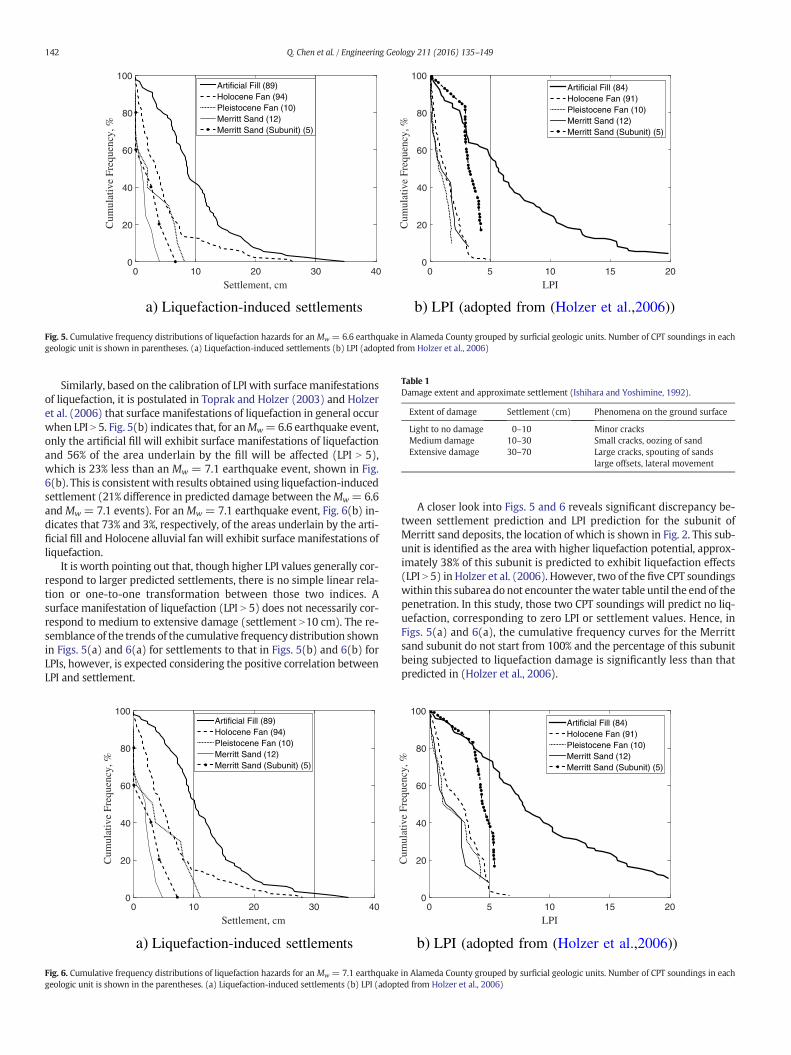
To estimate the hazard of liquefaction-induced settlement posed byeach geologic unit, settlement values at CPT soundingswere grouped bysurficial geologic unit. Cumulative frequency distributions of settle-ments are plotted in Fig. 5(a) for Mw = 6.6 earthquake and in Fig. 6(a)for Mw = 7.1 earthquake. In a previous analysis by Holzer et al.(2006), liquefaction potential index (LPI) were grouped by each geolog-ic unit and used as basis to assess liquefaction hazards posed by eachgeologic unit. Cumulative frequency distributions of LPIs from Holzeret al. (2006) are shown in Fig. 5(b) for Mw = 6.6 earthquake and Fig.6(b) for Mw = 7.1 earthquake for comparison with the current study.
The information presented in Figs. 5 and 6 can be used as an initialquantitative evaluation of liquefaction-induced settlements and the
a) Mw = 6.6 earthquake
Fig. 4. Cumulative frequency functions of liquefaction-induce
associated extent of damage (ref. Table 1) in each geologic unit. The per-centage of soundings underlain by a geologic unit that falls within a cer-tain settlement range may be used as an indication of the approximatepercentage of the surface area exhibiting the corresponding damagelevel. The more CPT soundings included, the better such an approxima-tion becomes.
Following such an interpretation, Fig. 5(a) predicts that, for anMw=6.6 earthquake event caused by the rupture of the south segmentof the Hayward Fault, 42% of the areas underlain by the artificial fill willexhibit medium to extensive damage, which is 21% less than an Mw =7.1 earthquake (Fig. 5(a)). Approximately 13% of the areas underlain bythe Holocene alluvial fan will exhibit medium to extensive damage.
For an Mw = 7.1 earthquake event, Fig. 6(a) indicates that approxi-mately 53% and 15% of the areas underlain by the artificial fill and theHolocene alluvial fan, respectively, will exhibit medium to extensivedamage. Medium to extensive damage is not anticipated for the areasunderlain by most of the Pleistocene alluvial fan deposits since onlyone of the ten CPT soundings in this geologic unit is predicted to havemedium damage. This site (numbered as OAK024 in the USGS database(USGS, 2015) and located at 37.792°−122.252° is underlain by the BullLake till, which is a softer subunit of Pleistocene fan deposits.Most of theMerritt sand are not anticipated to experience extensive damage either.
b) Mw = 7.1 earthquake
d settlements at 210 CPT soundings in Alameda County.
Settlement, cm0 10 20 30 40
Cum
ulat
ive
Freq
uenc
y, %
0
20
40
60
80
100Artificial Fill (89)Holocene Fan (94)Pleistocene Fan (10)Merritt Sand (12)Merritt Sand (Subunit) (5)
a) Liquefaction-induced settlements
LPI0 5 10 15 20
Cum
ulat
ive
Freq
uenc
y, %
0
20
40
60
80
100Artificial Fill (84)Holocene Fan (91)Pleistocene Fan (10)Merritt Sand (12)Merritt Sand (Subunit) (5)
b) LPI (adopted from (Holzer et al.,2006))
Fig. 5. Cumulative frequency distributions of liquefaction hazards for an Mw = 6.6 earthquake in Alameda County grouped by surficial geologic units. Number of CPT soundings in eachgeologic unit is shown in parentheses. (a) Liquefaction-induced settlements (b) LPI (adopted from Holzer et al., 2006)
Table 1Damage extent and approximate settlement (Ishihara and Yoshimine, 1992).
Extent of damage Settlement (cm) Phenomena on the ground surface
Light to no damage 0–10 Minor cracksMedium damage 10–30 Small cracks, oozing of sandExtensive damage 30–70 Large cracks, spouting of sands
Similarly, based on the calibration of LPI with surfacemanifestationsof liquefaction, it is postulated in Toprak and Holzer (2003) and Holzeret al. (2006) that surface manifestations of liquefaction in general occurwhen LPI N 5. Fig. 5(b) indicates that, for anMw=6.6 earthquake event,only the artificial fill will exhibit surface manifestations of liquefactionand 56% of the area underlain by the fill will be affected (LPI N 5),which is 23% less than an Mw = 7.1 earthquake event, shown in Fig.6(b). This is consistent with results obtained using liquefaction-inducedsettlement (21% difference in predicted damage between theMw =6.6and Mw = 7.1 events). For anMw = 7.1 earthquake event, Fig. 6(b) in-dicates that 73% and 3%, respectively, of the areas underlain by the arti-ficial fill and Holocene alluvial fan will exhibit surface manifestations ofliquefaction.
It is worth pointing out that, though higher LPI values generally cor-respond to larger predicted settlements, there is no simple linear rela-tion or one-to-one transformation between those two indices. Asurface manifestation of liquefaction (LPI N 5) does not necessarily cor-respond to medium to extensive damage (settlement N10 cm). The re-semblance of the trends of the cumulative frequencydistribution shownin Figs. 5(a) and 6(a) for settlements to that in Figs. 5(b) and 6(b) forLPIs, however, is expected considering the positive correlation betweenLPI and settlement.
Settlement, cm0 10 20 30 40
Cum
ulat
ive
Freq
uenc
y, %
0
20
40
60
80
100Artificial Fill (89)Holocene Fan (94)Pleistocene Fan (10)Merritt Sand (12)Merritt Sand (Subunit) (5)
a) Liquefaction-induced settlements
Fig. 6. Cumulative frequency distributions of liquefaction hazards for an Mw = 7.1 earthquakegeologic unit is shown in the parentheses. (a) Liquefaction-induced settlements (b) LPI (adopt
A closer look into Figs. 5 and 6 reveals significant discrepancy be-tween settlement prediction and LPI prediction for the subunit ofMerritt sand deposits, the location of which is shown in Fig. 2. This sub-unit is identified as the area with higher liquefaction potential, approx-imately 38% of this subunit is predicted to exhibit liquefaction effects(LPI N 5) in Holzer et al. (2006). However, two of the five CPT soundingswithin this subarea do not encounter thewater table until the end of thepenetration. In this study, those two CPT soundings will predict no liq-uefaction, corresponding to zero LPI or settlement values. Hence, inFigs. 5(a) and 6(a), the cumulative frequency curves for the Merrittsand subunit do not start from 100% and the percentage of this subunitbeing subjected to liquefaction damage is significantly less than thatpredicted in (Holzer et al., 2006).
LPI0 5 10 15 20
Cum
ulat
ive
Freq
uenc
y, %
0
20
40
60
80
100Artificial Fill (84)Holocene Fan (91)Pleistocene Fan (10)Merritt Sand (12)Merritt Sand (Subunit) (5)
b) LPI (adopted from (Holzer et al.,2006))
in Alameda County grouped by surficial geologic units. Number of CPT soundings in eached from Holzer et al., 2006)
a) Mw = 6.6 earthquake b) Mw = 7.1 earthquake
Fig. 7. Empirical and fitted semivariograms of liquefaction-induced settlements at CPT soundings in Alameda County (calculated with lag separate h = 105 m and 20% tolerance). (a)Mw = 6.6 earthquake (b) Mw = 7.1 earthquake.
143Q. Chen et al. / Engineering Geology 211 (2016) 135–149
5.3. Spatial analysis and mapping of liquefaction-induced settlements
Previous analysis focuses on the liquefaction-induced settlements atindividual CPT soundings. The probabilistic and cumulative frequencyplots are based on information at those isolated locations. To estimatethe extent of the liquefaction-induced settlements over a large region,the spatial correlation needs to be considered. In this section, the spatialdependence will be characterized through the semivariogram model,described in detail in Section 4.1. Multiscale random field models willthen be used to generate realizations of settlements throughout theregion.
The spatial structure of the liquefaction-induced settlements will beobtained from semivariogram inference. Given settlement predictionsat 210 CPT soundings and their spatial coordinates, the samplesemivariogram γðhÞ is computed as (Goovaerts, 1997)
γ hð Þ ¼ 12N hð Þ
XN hð Þ
α¼1
z uαð Þ−z uα þ hð Þ½ �2 ð34Þ
a) Single scale realization
Fig. 8. Typical random field realizations of liquefaction-induced settlements in Alameda CounSuperimposed grey lines correspond to boundaries of geologic units. (a) Single scale realizatio
whereN(h) is the number of pairs of data z located a vector h apart (i.e.,a lag binh). In the actual computation, a small tolerance (e.g., 10–20% ofthe distance h) is usually added to lag bins to accommodate unevenlyspaced sample points. Also, it is often convenient to use a scalar distancemeasure h, as defined in Eq. (26), for the calculation of semivariogram.
Fig. 7 shows the sample semivariogram based on settlements at 210CPT soundings for both Mw = 6.6 and Mw = 7.1 earthquake events.Given the sample semivariogram, a weighted least square method byCressie, 1985) is implemented to fit an analytical semivariogrammodel, shown as solid line in the plot.
As shown in Fig. 7, the empirical semivariograms for Mw = 6.6 andMw=7.1 earthquake events are almost identical, indicating a negligibleinfluence of earthquake intensity on the spatial structure of predictedsettlements. In this study, a common semivariogram model is fittedusing an exponential model of the form
γ hð Þ ¼ 1− exp −3ha
� �ð35Þ
b) Multiscale realization
ty for Mw = 6.6 earthquake event on the Hayward Fault. Unit of the settlement is in cm.n (b) Multiscale realization.
a) Single scale realization b) Multiscale realization
Fig. 9. Typical random field realizations of liquefaction-induced settlements in Alameda County for Mw = 7.1 earthquake event on the Hayward Fault. Unit of the settlement is in cm.Superimposed grey lines correspond to boundaries of geologic units. (a) Single scale realization (b) Multiscale realization.
where the practical range a = 2,400 m. This fitted semivariogram willbe used in the random field realization of settlements across the regionof interest.
In addition to the semivariogram, the random field model requiresthe probabilistic distribution of the variable of interest. Herein, apiece-wise linear probability density function is fitted to the histogramof predicted settlements in Fig. 3. A normal score mapping and a se-quential Gaussian simulation process are then used to generate randomfield realizations of variables of interest. Such simulation process hasbeen successfully applied in previous applications and it has beenshown that the spatial structure is preserved after normal score map-ping and during the simulation process (Baker and Faber, 2008; Bakeret al., 2011; Chen et al., 2012, 2015).
Figs. 8 and 9 plot the typical single andmultiscale random field real-izations of liquefaction-induced settlements for earthquake eventsMw = 6.6 and Mw = 7.1, respectively. In the multiscale realizations,higher resolutions are introduced in the artificial fill geologic unit,where higher liquefaction hazard is expected. It should be noted that,
a) Mw = 6.6 earthquake
Fig. 10. Typical histograms of simulated liquefaction-induced settlements acros
on average, the higher resolution region in a multiscale field resemblesthe trend seen in the single scale counterpart but with much more de-tailed information. Such higher resolution information is importantwhen performing local site-specific analysis, as will be shown later.
The corresponding histograms of simulated liquefaction-inducedsettlements are plotted in Fig. 10. The histograms have preserved thedistribution of settlements at 210 CPT locations as previously shownin Fig. 3. Moreover, the spatial structure is also found to be upheld dur-ing the simulation.
The random field model can be coupled with Monte Carlo simula-tions to evaluate various quantities of interest and associated uncer-tainties. As an example, the cumulative frequency distribution of thepredicted settlements are evaluated alongwith uncertainties in the pre-diction. Fig. 11 shows the cumulative frequency of the predicted settle-ments based on a total of 1000 Monte Carlo simulations. The error bar(±one standard deviation) is also included in the cumulative frequencyplots. It can be seen that, for the given earthquake events, less than 30%of the Alameda County area is predicted to have a settlement greater
b) Mw = 7.1 earthquake
s the Alameda County. (a)Mw = 6.6 earthquake (b)Mw = 7.1 earthquake.
a) Mw = 6.6 earthquake b) Mw = 7.1 earthquake
Fig. 11. Cumulative frequency plots of the liquefaction-induced settlements, calculated from 1000 Monte Carlo simulations. (a)Mw = 6.6 earthquake (b) Mw = 7.1 earthquake.
145Q. Chen et al. / Engineering Geology 211 (2016) 135–149
than 10 cm. The percentage of area predicted to have more than 30 cmsettlement is very close to zero. A comparison between the single andmultiscale results in Fig. 11 reveals a similar trend but consistentlyhigher predictionswithmultiscale. For example, for theMw=7.1 earth-quake, the multiscale result indicates that about 27% of the area has asettlement exceeding 10 cm,while the single scale predicts the percent-age to be 18%. Since the single (coarse) scale is defined as the average ofthe corresponding fine scale elements as in Eq. (27), the findings in Fig.11 indicate that such averaging process might yield an unconservativeestimation of liquefaction hazard.
To further demonstrate the capability of random field models andexplore their potential applications combinedwithMonte Carlo simula-tions, we re-analyze the cumulative frequency distributions of liquefac-tion-induced settlements grouped by different geologic units, aspreviously presented in Section 5.2. Instead of using just settlementsat CPT soundings, herein, the cumulative frequency distributions areevaluated using settlements throughout Alameda County based on re-sults of 1000 Monte Carlo simulations. The results are summarized inFig. 12 for bothMw = 6.6 and Mw = 7.1 earthquake events.
ForMw=6.6 earthquake, Fig. 12(a) indicates that 48.2% of the areasunderlain by artificial fill and 7.4% of the areas underlain by Holocene
Fig. 12. Cumulative frequency distributions of predicted liquefaction-induced settlements aearthquakes on the Hayward Fault. (a)Mw = 6.6 earthquake (b) Mw = 7.1 earthquake.
alluvial fanwill exhibit medium to extensive damage (settlement great-er than 10 cm). The combined region underlain by Merritt sand Pleisto-cene fan and the northeast portion of the Holocene fan is predicted tohave 10% of its area exhibiting medium damage. Only 1% of the subareaunderlain byMerritt sand has a medium damage prediction. These pre-dictions are consistent with those made in Section 5.2.
For Mw = 7.1 earthquake, Fig. 12(b) indicates that 57.7% and13.2% , respectively, of the areas underlain by artificial fill and Holo-cene alluvial fan will exhibit medium to extensive damage. Thesepredictions are very close to the results in Section 5.2, which is 53%and 15%. The combined region underlain byMerritt sand, Pleistocenefan (also including the northeast portion of the Holocene fan) is pre-dicted to have less than 2.4% of its area exhibiting medium damage,which is negligible and again, consistent with predictions made inSection 5.2.
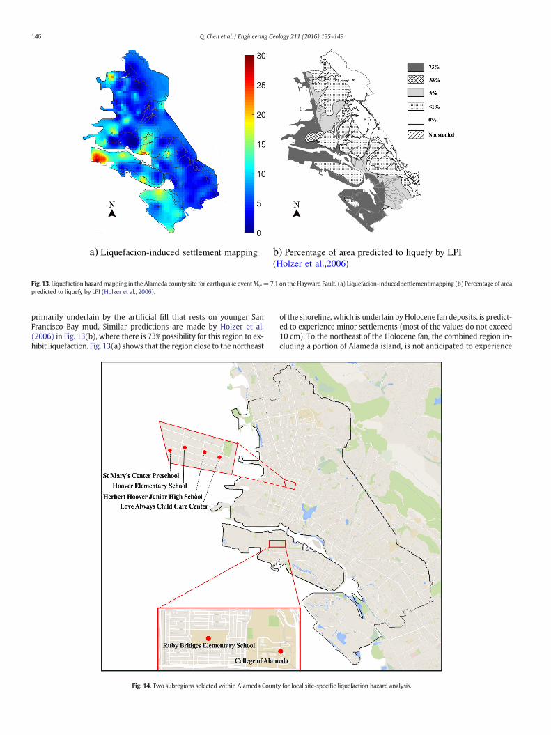
A visualization of the predicted liquefaction-induced settlementmapping, averaged from 1000 Monte Carlo simulations, is shown inFig. 13(a) along with the LPI mapping obtained from Holzer et al.(2006) shown in Fig. 13(b) for Mw = 7.1 earthquake event. As shownin Fig. 13(a), higher settlements (greater than 10 cm) occurs mainly inthe southwest region of the original natural shoreline, which is
cross Alameda County, grouped by surficial geologic units for Mw = 6.6 and Mw = 7.1
a) Liquefacion-induced settlement mapping b) Percentage of area predicted to liquefy by LPI(Holzer et al.,2006)
Fig. 13. Liquefaction hazardmapping in the Alameda county site for earthquake eventMw=7.1 on theHayward Fault. (a) Liquefacion-induced settlementmapping (b) Percentage of areapredicted to liquefy by LPI (Holzer et al., 2006).
primarily underlain by the artificial fill that rests on younger SanFrancisco Bay mud. Similar predictions are made by Holzer et al.(2006) in Fig. 13(b), where there is 73% possibility for this region to ex-hibit liquefaction. Fig. 13(a) shows that the region close to the northeast
Fig. 14. Two subregions selected within Alameda Count
of the shoreline, which is underlain by Holocene fan deposits, is predict-ed to experience minor settlements (most of the values do not exceed10 cm). To the northeast of the Holocene fan, the combined region in-cluding a portion of Alameda island, is not anticipated to experience
y for local site-specific liquefaction hazard analysis.
a) Mw = 6.6 earthquake b) Mw = 7.1 earthquake
Fig. 15. Fraction of area exceeding a particular settlement for the Ruby Bridges School and Hoover School sites. (a) Mw = 6.6 earthquake (b)Mw = 7.1 earthquake.
147Q. Chen et al. / Engineering Geology 211 (2016) 135–149
high settlements. This region is mainly underlain by Merritt sand andPleistocene fan deposits.
While the results show that the proposed framework predicts con-sistent liquefaction hazards for the entire region and for individual sur-ficial geologic units, the multiscale random field models provide muchmore detailed information and are able account for spatial variabilityof the settlementwithin each geologic unit. This enables the assessmentof local site-specific liquefaction hazards. To demonstrate this point, twolocal sites shown in Fig. 14 are picked from Alameda County. The firstsite is located on Alameda Island, consisting of Ruby Bridges ElementarySchool, the College of Alameda and a crowded residential area. This sitewill be referred to as the “Ruby Bridges School” site in the followinganalysis. The second local site, which includes schools and care centerssuch as St. Mary's Center Preschool, Hoover Elementary School, HerbertHoover Junior High School and Love Always Child Care Center, will bereferred to as the “Hoover School” site in the following analysis. The as-sessment is based on the same 1000 Monte Carlo simulations per-formed and used in previous cumulative frequency plots.
Fig. 15 shows the percentage of area predicted to exceed certain set-tlement values. It can be seen that 58% of the Ruby Bridges School sitewill suffer medium to extensive damage (settlement N 10 cm) for theMw = 6.6 earthquake event, while the percentage is only 3% for theHoover School site. For an Mw = 7.1 earthquake event, 75% of the
a) Mw = 6.6 earthquake
Fig. 16. Percentage of area that will suffer medium to extensive damage (settlement N 10 cm)Mw = 6.6 earthquake (b) Mw = 7.1 earthquake.
Ruby Bridges School site and 9%of theHoover School sitewill sufferme-dium to extensive damage.
Fig. 16 plots the percentage of area that will suffermedium to exten-sive damage and the corresponding probabilities for bothMw=6.6 andMw = 7.1 earthquake events for two sites. Again, the Ruby BridgesSchool site is expected to suffer more liquefaction-induced damage(quantified by the predicted settlements) than the Hoover School site.Such detailed information demonstrates the potential of the multiscalerandom field models for local site-specific liquefaction hazard analysis.
6. Conclusions
In this paper, a framework is developed that integrates the classicalCPT-based liquefaction model with multiscale random field modelsand Monte Carlo simulations for the probabilistic and spatial assess-ment of liquefaction-induced settlements over a region and acrossscales. One critical advantage of the developed framework is its abilityto consistently refine and provide settlement estimations across differ-ent scales, from regional and surficial geologic unit scale all the way tolocal site-specific scale. The developed framework is applied to the liq-uefaction hazard analysis of the Alameda County site in California andis demonstrated to be a valuable tool formultiscale regional liquefactionhazard analysis. In summary, it is found that
b) Mw = 7.1 earthquake
vs. corresponding probabilities for the Ruby Bridges School and Hoover School sites. (a)
1. Quantitatively consistent liquefaction hazards over the entire studiedregion andwithin each surficial geologic unit are obtainedwhen ver-ified against existing analysis and knowledge of the studied region.
2. Spatial variability of soil properties within each geologic unit acrossdifferent scales is captured, which provides a way to systematicallyrefine and perform local site-specific liquefaction analysis while pre-serving the liquefaction hazard prediction at the regional scale.
3. The spatial structure of the predicted settlements inferred fromavail-able field data is shown to be relatively insensitive to the earthquakeshaking intensity considered in this study (Mw = 6.6 andMw =7.1)and such inferred spatial structure is preserved during the randomfield modeling process.
4. In the Alameda County site, the artificial fill is the surficial geologicunit most susceptible to liquefaction hazard (48.2% and 57.7% ofthe area will exhibit medium to extensive damage for the Mw =6.6 and Mw = 7.1 earthquake scenarios considered) followed bythe Holocene alluvial fan deposits (the corresponding percentagesare 7.4% and 13.2%).
5. Local site-specific analysis shows that the Ruby Bridges School site isexpected to suffer more liquefaction-induced damage (quantified bythe predicted settlements) than the Hoover School site.Future work will fully incorporate uncertainties in the liquefactionsettlement models, the input parameters, and the earthquake shak-ing intensities, and will explore the effect of these uncertainties inthe regional liquefaction hazard analysis. Further validation of the es-timated settlements from the proposed model against field observa-tions from major earthquakes in this region (e.g., the 1989 LomaPrieta earthquake) is warranted.
Acknowledgment
Clemson University is acknowledged for the generous allotment ofcompute time on the Palmetto cluster. The authors thank AndrewBrownlow from Clemson University for proofreading and providingcritical feedback to the paper. The expert reviews from three anony-mous reviewers are also gratefully acknowledged.
Bartlett, S.F., Gerber, T.M., Hinckley, D., 2007. Probabilistic liquefaction potential and liq-uefaction-induced ground failure maps for the urban Wasatch Front: phase IV. Tech-nical Report Awards 07HQGR0021 and 07HQGR0024, Technical Report Submitted tothe United States Geological Survey.
Chen, Q., Seifried, A., Andrade, J.E., Baker, J.W., 2012. Characterization of random fields andtheir impact on the mechanics of geosystems at multiple scales. Int. J. Numer. Anal.Methods Geomech. 360 (2), 140–165.
Chen, Q., Wang, C., Juang, C.H., 2015. CPT-based evaluation of liquefaction potential ac-counting for soil spatial variability at multiple scales. J. Geotech. Geoenviron.04015077.
Cressie, N., 1985d. Fitting variogrammodels by weighted least squares. J. Int. Assoc. Math.Geol. 170 (5), 563–586.
Goovaerts, P., 1997. Geostatistics for Natural Resources Evaluation. Oxford UniversityPress, New York.
Gringarten, E., Deutsch, C.V., 2001. Teacher's aide variogram interpretation and modeling.Math. Geol. 330 (4), 507–534.
Helley, E.J., Graymer, R.W., 1997. Quaternary geology of Alameda County, and parts ofContra Costa, Santa Clara, San Mateo, San Francisco, Stanislaus, and San Joaquincounties, California: a digital database. Technical Report 97–97, U.S. Geological SurveyOpen-File Report.
Hinckley, D.W., 2010. Liquefaction-induced ground displacement mapping for the SaltLake Valley, Utah. The University of Utah (PhD thesis).
Holzer, T.L., Bennett, M.J., Noce, T.E., Padovani, A.C., Tinsley III, J.C., 2006. Liquefaction haz-ardmappingwith LPI in the greater Oakland, California, area. Earthquake Spectra 220(3), 693–708.
Ishihara, K., Yoshimine, M., 1992. Evaluation of settlements in sand deposits following liq-uefaction during earthquakes. Soils Found. 320 (1), 173–188.
Iwasaki, T., Tatsuoka, F., Tokida, K., Yasuda, S., 1978. A practical method for assessing soilliquefaction potential based on case studies at various sites in Japan. Proceedings 2ndInternational Conference on Microzonation, pp. 885–896.
Iwasaki, T., Tokida, K., Tatsuoka, F., Watanabe, S., Yasuda, S., Sato, H., 1982. Microzonationfor soil liquefaction potential using simplified methods. Proceedings of the 3rd Inter-national Conference on Microzonation, Seattle vol. 3, pp. 1310–1330.
Juang, C.H., Li, D.K., Fang, S.Y., Liu, Z., Khor, E.H., 2008a. Simplified procedure for develop-ing joint distribution of amax and Mw for probabilistic liquefaction hazard analysis.J. Geotech. Geoenviron. 1340 (8), 1050–1058.
Juang, C.H., Liu, C.N., Chen, C.H., Hwang, J.H., Lu, C.C., 2008b. Calibration of liquefaction po-tential index: a re-visit focusing on a new CPTU model. Eng. Geol. 1020 (1), 19–30.
Juang, C.H., Ching, J., Wang, L., Khoshnevisan, S., Ku, C.S., 2013. Simplified procedure forestimation of liquefaction-induced settlement and site-specific probabilistic settle-ment exceedance curve using cone penetration test (CPT). Can. Geotech. J. 500(10), 1055–1066.
Ku, C.S., Juang, C.H., Chang, C.W., Ching, J., 2012. Probabilistic version of the robertson andwride method for liquefaction evaluation: development and application. Can.Geotech. J. 490 (1), 27–44.
Lee, C.Y., 2007. Earthquake-induced settlements in saturated sandy soils. ARPN J. Eng.Appl. Sci. 20 (4), 6–13.
Lee, K.L., Albaisa, A., 1974. Earthquake induced settlements in saturated sands. J. Geotech.Eng. Div. ASCE 1000 (4), 387–406.
Lenz, J.A., Baise, L.G., 2007. Spatial variability of liquefaction potential in regional mappingusing CPT and SPT data. Soil Dyn. Earthq. Eng. 270 (7), 690–702.
Lu, C.C., Hwang, J.H., Juang, C.H., Ku, C.S., Luo, Z., 2009. Framework for assessing probabil-ity of exceeding a specified liquefaction-induced settlement at a given site in a givenexposure time. Eng. Geol. 1080 (1), 24–35.
Nagase, H., Ishihara, K., 1988. Liquefaction-induced compaction and settlement of sandduring earthquakes. Soils Found. 280 (1), 65–76.
Papathanassiou, G., Pavlides, S., Ganas, A., 2005. The 2003 lefkada earthquake: Field obser-vations and preliminary microzonation map based on liquefaction potential index forthe town of Lefkada. Eng. Geol. 820 (1), 12–31.
Pradel, D., 1998. Procedure to evaluate earthquake-induced settlements in dry sandysoils. J. Geotech. Geoenviron. 1240 (4), 364–368.
Robertson, P.K., 2009. Performance based earthquake design using the CPT. Proc. IS-Tokyo, pp. 3–20.
Robertson, P.K., Wride, C.E., 1998. Evaluating cyclic liquefaction potential using the conepenetration test. Can. Geotech. J. 350 (3), 442–459.
Shamoto, Y., Zhang, J.M., Tokimatsu, K., 1998. Methods for evaluating residual post-lique-faction ground settlement and horizontal displacement. Soils Found. 38, 69–84.
Sonmez, H., 2003. Modification of the liquefaction potential index and liquefaction sus-ceptibility mapping for a liquefaction-prone area (Inegol, Turkey). Environ. Geol.440 (7), 862–871.
Sonmez, H., Gokceoglu, C., 2005. A liquefaction severity index suggested for engineeringpractice. Environ. Geol. 480 (1), 81–91.
Sowers, J.M., Richard, C.M., 2010. Creek & Watershed Map of Oakland and Berkeley. Oak-land Museum of California.
Thompson, E.M., Baise, L.G., Kayen, R.E., 2007. Spatial correlation of shear-wave velocity inthe San Francisco Bay Area sediments. Soil Dyn. Earthq. Eng. 270 (2), 144–152.
Tokimatsu, K., Seed, H.B., 1984. Simplified procedures for the evaluation of settlements inclean sands. Technical Report CB/EERC-84/16. Earthquake Engineering Research Cen-ter, University of California.
Tokimatsu, K., Seed, H.B., 1987. Evaluation of settlements in sands due to earthquakeshaking. J. Geotech. Eng. 1130 (8), 861–878.
Toprak, S., Holzer, T.L., 2003. Liquefaction potential index: field assessment. J. Geotech.Geoenviron. 1290 (4), 315–322.
Trask, P., Rolston, J., 1951. Engineering geology of San Francisco Bay, California. Geol. Soc.Am. Bull. 620 (9), 1079–1110.
Tsukamoto, Y., Ishihara, K., 2010. Analysis on settlement of soil deposits following lique-faction during earthquakes. Soils Found. 500 (3), 399–411.
Tsukamoto, Y., Ishihara, K., Sawada, S., 2004. Settlement of silty sand deposits followingliquefaction during earthquakes. Soils Found. 440 (5), 135–148.
USGS, 2014. U.S. Geological Survey National Seismic Hazard Maps. http://earthquake.usgs.gov/hazards/products/conterminous/2014/data/.
USGS, 2015. U.S. Geological Survey Hazards Program CPT database. http://earthquake.usgs.gov/research/cpt/.
Valverde-Palacios, I., Vidal, F., Valverde-Espinosa, I., Martn-Morales, M., 2014. Simplifiedempirical method for predicting earthquake-induced settlements and its applicationto a large area in spain. Eng. Geol. 181, 58–70.
van Ballegooy, S., Wentz, F., Boulanger, R.W., 2015. Evaluation of CPT-based liquefactionprocedures at regional scale. Soil Dyn. Earthq. Eng. 79, 315–334.
Vivek, B., Raychowdhury, P., 2014. Probabilistic and spatial liquefaction analysis using CPTdata: a case study for Alameda County site. Nat. Hazards 710 (3), 1715–1732.
149Q. Chen et al. / Engineering Geology 211 (2016) 135–149
WGCEP, 2003. Earthquake probabilities in the San Francisco Bay region 2002–2031: asummary of findings. Technical Report U.S. Geological Survey Open-file Report 03–214. United States Geological Survey.
Wu, J., Seed, R.B., 2004. Estimation of liquefaction-induced ground settlement (case stud-ies). Proceedings of the 5th International Conference on Case Histories in Geotechni-cal Engineering number 6. Springer.
Yoshimine, M., Nishizaki, H., Amano, K., Hosono, Y., 2006. Flow deformation of liquefiedsand under constant shear load and its application to analysis of flow slide of infiniteslope. Soil Dyn. Earthq. Eng. 260 (2), 253–264.
Youd, T.L., Idriss, I.M., Andrus, R.D., Arango, I., Castro, G., Christian, J., Dobry, R., Finn,D.W.L., Harder Jr., L.F., Hynes, M.E., Ishihara, K., Koester, J., Liao, S., Marcuson, W.I.,
Martin, G., Mitchell, J., Moriwaki, Y., Power, M., Robertson, P., Seed, R., Stokoe, K.I.,2001. Liquefaction resistance of soils: summary report from the 1996 NCEER and1998 NCEER/NSF workshops on evaluation of liquefaction resistance of soils.J. Geotech. Geoenviron. 1270 (4), 297–313.