ORI GIN AL PA PER

Probabilistic assessment of wildfire hazardand municipal watershed exposure

Joe Scott • Don Helmbrecht • Matthew P. Thompson • David E. Calkin •

Kate Marcille

Received: 5 April 2012 / Accepted: 20 June 2012 / Published online: 12 July 2012� US Government 2012

Abstract The occurrence of wildfires within municipal watersheds can result in signif-

icant impacts to water quality and ultimately human health and safety. In this paper, we

illustrate the application of geospatial analysis and burn probability modeling to assess the

exposure of municipal watersheds to wildfire. Our assessment of wildfire exposure consists

of two primary components: (1) wildfire hazard, which we characterize with burn proba-

bility, fireline intensity, and a composite index, and (2) geospatial intersection of watershed

polygons with spatially resolved wildfire hazard metrics. This effort enhances investigation

into spatial patterns of fire occurrence and behavior and enables quantitative comparisons

of exposure across watersheds on the basis of a novel, integrated measure of wildfire

hazard. As a case study, we consider the municipal watersheds located on the Beaverhead-

Deerlodge National Forest (BDNF) in Montana, United States. We present simulation

results to highlight exposure across watersheds and generally demonstrate vast differences

in fire likelihood, fire behavior, and expected area burned among the analyzed municipal

watersheds. We describe how this information can be incorporated into risk-based strategic

fuels management planning and across the broader wildfire management spectrum. To

conclude, we discuss strengths and limitations of our approach and offer potential future

expansions.

Keywords Wildfire � Hazard analysis � Exposure analysis � Fire modeling �Municipal watersheds

J. ScottPyrologix LLC, Missoula, MT 59801, USA

D. HelmbrechtTEAMS Enterprise Unit, US Forest Service, Missoula, MT 59807, USA

M. P. Thompson (&) � D. E. CalkinRocky Mountain Research Station, US Forest Service, Missoula, MT 59807, USAe-mail: mpthompson02@fs.fed.us

K. MarcilleOregon State University, Corvallis, OR 97331, USA

123

Nat Hazards (2012) 64:707–728DOI 10.1007/s11069-012-0265-7

1 Introduction

In this paper, we illustrate the application of geospatial analysis and burn probability

modeling to assess wildfire hazard and exposure of municipal watersheds (i.e., drinking

water supplies) to wildfire. Wildfires can have profound effects on watersheds (Parise and

Cannon 2012), and sediment loads from burned watersheds have resulted in shutdowns of

municipal water supply facilities due to water quality (Ryan and Samuels 2010). Thus,

there are pressing human health and safety reasons for identifying at-risk watersheds. As a

case study, we consider the municipal watersheds located on the Beaverhead-Deerlodge

National Forest (BDNF) in Montana, United States. Our assessment of wildfire exposure

consists of two primary components: (1) wildfire hazard, which we characterize with burn

probability, fireline intensity, and a composite index, and (2) geospatial intersection of

watershed polygons with spatially resolved wildfire hazard metrics.

1.1 Background: wildfire hazard and risk analysis

Federal wildfire management within the United States is increasingly adopting risk-based

paradigms to inform policy and management (Calkin et al. 2011a; Fire Executive Council

2009). Recently published examples include strategic national-scale assessments

(Thompson et al. 2011a), fuel treatment evaluation (Ager et al. 2010), incident-level

decision support (Calkin et al. 2011b; Noonan-Wright et al. 2011), and localized

assessment of risk to structures in the wildland–urban interface (Bar Massada et al.

2009). Advancements in computing power, fire behavior modeling, and geospatial data

acquisition and management enable spatially explicit simulation of where fire is likely to

ignite, spread, and interact with highly valued resources and assets (Finney et al. 2011;

Finney 2002). Applications of burn probability modeling techniques are still emerging,

with enormous potential for risk-based, strategic fire and fuels management (Miller et al.

2008).

Wildfire hazard is defined here as a physical situation with the potential for wildfire to

cause damage. Qualitatively, hazard can be described by the fire environment surrounding

the resource, for instance the fuel, weather, topography, and ignition characteristics.

Quantitatively, hazard can be described as the probability distribution of a fire charac-

teristic, usually wildfire intensity. A location likely to burn with high intensity, in this

modeling approach, has high hazard. Hazard, however, is but one component of wildfire

risk. Finney (2005) provides a quantitative definition of wildfire risk that integrates

information on burn likelihood, fire intensity, and magnitude of resource response to fire.

This approach aligns with ecological risk assessment paradigms premised on the analysis

of exposure and effects (Fairbrother and Turnley 2005). Wildfire exposure analysis typi-

cally explores the possible spatial interactions of fire-susceptible resources with fire

occurrence and behavior metrics, and fire effects analysis explores the potential magnitude

of wildfire-caused damages (Thompson and Calkin 2011). Conversely, for fire-adapted

ecosystems, exposure and effects analysis could highlight where fire may play an eco-

logically beneficial role and be promoted. Assessing risk informs decision making by

integrating and synthesizing information regarding the likelihood and magnitude of

impacts to resources (Sikder et al. 2006). This information can be used to help plan risk

mitigation activities across the wildfire management spectrum, including ignition pre-

vention efforts, proactive hazardous fuels reduction, suppression response planning, and

evacuation planning (Dennison et al. 2007).

708 Nat Hazards (2012) 64:707–728

123

1.2 Wildfire impacts to watershed health and integrity

Watersheds play important ecological, social, and economic roles and can potentially be

affected by a multitude of human and natural disturbances (Brauman et al. 2007; Brown

2000; Neary et al. 2005). Consideration of watershed health and integrity across the forest

is important for numerous reasons. Forests and federal lands, particularly in the Western

United States, are important providers of the water supply (Brown et al. 2008; Ryan and

Samuels 2010). Ecologically, watersheds have the potential to be greatly impacted by

wildland fire, and the results are often far-reaching. The natural occurrence of fire on the

landscape is an important component of watershed health and may have beneficial effects

in the long run (e.g., increased biodiversity) and functions as an agent of recovery (Benda

et al. 2003). However, fire can also induce dramatic and negative changes to watershed

integrity through flooding, debris flow, and subsequent impacts on human lives and spe-

cies’ habitat suitability. Post-fire effects can range in magnitude and impact, across time

and space, from rejuvenation of alluvial fans to burial of existing habitat (Benda et al.

2003). Post-fire floods and high sediment flow are of high concern (Neary et al. 2005).

Areas that have been naturally disturbed (i.e., post-fire environment) become more sus-

ceptible to substantial human degradation (Brown and Binkley 1994).

Erosion and sediment redistribution are commonly referenced as prominent effects of

fire on watersheds (Brown and Froemke 2010; Calkin et al. 2007; Shakesby and Doerr

2006; Brown 2000; Brown and Binkley 1994; Agee 1993). Stand-replacing fires (high

severity) often result in intense erosion and large influxes of sediment (Benda et al. 2003)

and woody debris in stream channels and confluences (Neary et al. 2005; Benda et al.

2003; Brown 2000) as well as shift overland flow rates and runoff behavior (Shakesby and

Doerr 2006). Debris flows are a potential response of recently burned basins and are

considered more severe than sediment-laden floods (Cannon et al. 2010). Fire severity is a

major determinant of impacts to soil and water resources (Shakesby and Doerr 2006; Neary

et al. 2005).

Our interest here is in wildfire impacts as they relate to municipal watersheds; readers

wishing for a more thorough review of hydrologic, geomorphic, and aquatic habitat-related

effects of wildfire are referred to Parise and Cannon (2012), Rieman et al. (2010), Moody

and Martin (2009), Dunham et al. (2007), Shakesby and Doerr (2006), Neary et al. (2005),

and Bisson et al. (2003). Municipal watersheds are critical infrastructure and disruption of

their operation can have serious economic and public safety consequences (Ryan and

Samuels 2010); hence, their explicit consideration within decision support systems sup-

porting incident management (Calkin et al. 2011b) and within strategic risk assessments

(Thompson et al. 2011a, b). Municipal water is affected by wildland fire occurrence and

management practices associated with fire (Brown 2000). Threats to drinking water from

wildfire are varied and can occur while a fire burns, from aerial application of fire retardant

(Neary et al. 2005; Ryan and Samuels 2010), or in the months and years following a fire

due to increased storm runoff (Shakesby and Doerr 2006), ash accumulation, and accel-

erated soil erosion and sedimentation (Emelko et al. 2011; Smith et al. 2010).

1.3 Case study description: BDNF wildfire hazard assessment

The study area for the assessment of watershed exposure included the approximately

3.2 million ha (8 million acres) in 12 BDNF planning units (called ‘‘landscapes’’ in the

Forest plan; see Fig. 1). The study area is less fire-prone than many other landscapes in the

western United States, but wildfire is nevertheless a concern. Our analysis sought to

Nat Hazards (2012) 64:707–728 709

123

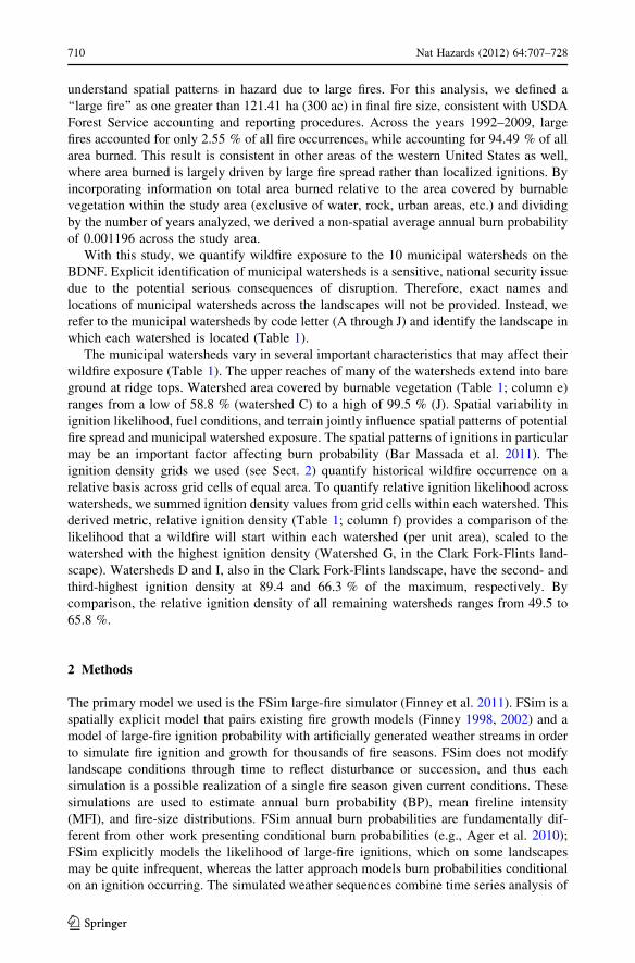
understand spatial patterns in hazard due to large fires. For this analysis, we defined a

‘‘large fire’’ as one greater than 121.41 ha (300 ac) in final fire size, consistent with USDA

Forest Service accounting and reporting procedures. Across the years 1992–2009, large

fires accounted for only 2.55 % of all fire occurrences, while accounting for 94.49 % of all

area burned. This result is consistent in other areas of the western United States as well,

where area burned is largely driven by large fire spread rather than localized ignitions. By

incorporating information on total area burned relative to the area covered by burnable

vegetation within the study area (exclusive of water, rock, urban areas, etc.) and dividing

by the number of years analyzed, we derived a non-spatial average annual burn probability

of 0.001196 across the study area.

With this study, we quantify wildfire exposure to the 10 municipal watersheds on the

BDNF. Explicit identification of municipal watersheds is a sensitive, national security issue

due to the potential serious consequences of disruption. Therefore, exact names and

locations of municipal watersheds across the landscapes will not be provided. Instead, we

refer to the municipal watersheds by code letter (A through J) and identify the landscape in

which each watershed is located (Table 1).

The municipal watersheds vary in several important characteristics that may affect their

wildfire exposure (Table 1). The upper reaches of many of the watersheds extend into bare

ground at ridge tops. Watershed area covered by burnable vegetation (Table 1; column e)

ranges from a low of 58.8 % (watershed C) to a high of 99.5 % (J). Spatial variability in

ignition likelihood, fuel conditions, and terrain jointly influence spatial patterns of potential

fire spread and municipal watershed exposure. The spatial patterns of ignitions in particular

may be an important factor affecting burn probability (Bar Massada et al. 2011). The

ignition density grids we used (see Sect. 2) quantify historical wildfire occurrence on a

relative basis across grid cells of equal area. To quantify relative ignition likelihood across

watersheds, we summed ignition density values from grid cells within each watershed. This

derived metric, relative ignition density (Table 1; column f) provides a comparison of the

likelihood that a wildfire will start within each watershed (per unit area), scaled to the

watershed with the highest ignition density (Watershed G, in the Clark Fork-Flints land-

scape). Watersheds D and I, also in the Clark Fork-Flints landscape, have the second- and

third-highest ignition density at 89.4 and 66.3 % of the maximum, respectively. By

comparison, the relative ignition density of all remaining watersheds ranges from 49.5 to

65.8 %.

2 Methods

The primary model we used is the FSim large-fire simulator (Finney et al. 2011). FSim is a

spatially explicit model that pairs existing fire growth models (Finney 1998, 2002) and a

model of large-fire ignition probability with artificially generated weather streams in order

to simulate fire ignition and growth for thousands of fire seasons. FSim does not modify

landscape conditions through time to reflect disturbance or succession, and thus each

simulation is a possible realization of a single fire season given current conditions. These

simulations are used to estimate annual burn probability (BP), mean fireline intensity

(MFI), and fire-size distributions. FSim annual burn probabilities are fundamentally dif-

ferent from other work presenting conditional burn probabilities (e.g., Ager et al. 2010);

FSim explicitly models the likelihood of large-fire ignitions, which on some landscapes

may be quite infrequent, whereas the latter approach models burn probabilities conditional

on an ignition occurring. The simulated weather sequences combine time series analysis of

710 Nat Hazards (2012) 64:707–728

123

the fire danger rating index Energy Release Component (ERC) and corresponding fuel

moisture scenario with historic joint distributions of wind speed and direction. For use in

FSim, empirical distribution functions that relate daily ERC values to large-fire occurrence

for the fire modeling area were developed in FireFamilyPlus (Rocky Mountain Research

Station Fire Sciences Laboratory and Systems for Environmental Management 2002). Fire

Fig. 1 Overview of the analysis area for the assessment of wildfire hazard and watershed exposure on theBeaverhead-Deerlodge National Forest, showing 12 planning units (‘‘landscapes’’ as identified in the Forestplan), listed alphabetically: Big Hole, Boulder River, Clark Fork-Flints, Elkhorn, Gravelly, Jefferson River,Lima-Tendoy, Madison, Pioneer, Tobacco Roots, Upper Clark Fork, and Upper Rock Creek. The 10municipal watersheds of interest are found across these 12 BDNF landscapes (Table 1). National ForestSystem lands are shown in cross-hatching

Nat Hazards (2012) 64:707–728 711

123

duration is not fixed within FSim, but rather is determined by the artificially generated

weather stream and an embedded suppression algorithm (Finney et al. 2009).To minimize

edge effects, we allowed simulated fires to move into the analysis area from adjacent land

by including a 8-km (5-mile) buffer from the edge of any landscape to the extent of our

geospatial data. The total fire modeling area encompasses 6,103,188 ha (15,080,978 acres),

and using a 90 m pixel resolution, this resulted in a modeling landscape of 2,415 9 3,120

pixels.

Figure 2 presents a simplified flowchart for our wildfire exposure analysis process, with

the key analytical steps highlighted in gray. In the following subsections, we describe our

methods for creating the necessary input files for FSim and for performing the wildfire

exposure analysis with FSim. Specifically, this entailed generating information on land-

scape characteristics such as terrain and fuel conditions (§2.1), acquiring weather data for

generating artificial fire seasons (§2.2), obtaining fire occurrence data and developing

probabilistic large-fire occurrence relationships (§2.3), and running the model to charac-

terize pixel-based wildfire hazard within municipal watersheds (§2.4).

2.1 Generation of landscape file for fire simulation model

In order to simulate fire growth and behavior, FSim requires a user-defined landscape file,

which consists of geospatial data representing terrain, fuel, and vegetation characteristics.

Terrain characteristics include slope steepness, aspect, and elevation. Fuel characteristics

include surface fire behavior fuel model, forest canopy base height, and forest canopy bulk

density. Vegetation characteristics include forest canopy cover and forest canopy height.

LANDFIRE (www.landfire.gov) is a valuable source for such data; however, a few

challenges existed when applying LANDFIRE’s off-the-shelf landscape data for this mid-

scale assessment. First, the fire modeling area includes portions of four LANDFIRE

mapping zones, resulting in data discontinuities (seamlines) at mapping zone boundaries.

This occurred if the LANDIFRE rules for assigning and mapping fuel characteristics (i.e.,

Table 1 Characteristics of the ten municipal watersheds on the Beaverhead-Deerlodge National Forest

(a)Watershed

(b)BDNF landscape

(c)Total watershed

area (ha)

(d)Burnable

watershedarea (ha)

(e)Burnable area

(% of totalwatershed)

(f)Relative ignition

density (%)

A Boulder River 10,779 10,093 93.6 60.3

B Upper Clark Fork 3,144 3,115 99.1 54.6

C Jefferson River 885 521 58.8 52.5

D Clark Fork-Flints 788 722 91.6 89.4

E Tobacco Roots 3,021 2,494 82.5 65.8

F Pioneer 6,425 5,930 92.3 58.3

G Clark Fork-Flints 1,593 1,580 99.2 100.0

H Big Hole 1,290 1,264 98.0 49.5

I Clark Fork-Flints 1,812 1,303 71.9 66.3

J Upper Clark Fork 1,337 1,330 99.5 57.5

Non-burnable watershed area consists of bare ground at the upper reaches of the watersheds. Relativeignition density (column f) is an indicator of the relative potential for fire starts within the watersheds.Because the ignition density grid used to produce these data is coarse (see Fig. 2), relative ignition density inthe area surrounding the watersheds should be similar to the values reported here

712 Nat Hazards (2012) 64:707–728

123

surface fire behavior fuel model, canopy base height, and canopy bulk density) differed

between zones. Rules for mapping fuel characteristics are based on the combinations of

existing vegetation type (EVT), existing vegetation cover (EVC), existing vegetation

height (EVH), and biophysical setting (BpS). Second, rules for mapping fuel character-

istics are generalized to whole LANDFIRE mapping zones, which span millions of hect-

ares each. Rules that account for variability across a whole mapping zone can result in

imprecision when looking at just a small portion of the mapping zone. Third, LANDFIRE’s

published forest canopy cover data available at the time were known to overestimate this

factor (this overestimate has since been corrected and is not present in recent versions of

LANDFIRE data).

For these reasons, we held a local fuel calibration workshop with BDNF fire and fuel

staff to produce seamless, locally calibrated surface and canopy fuel data based on

LANDFIRE data version 1.0.0 of EVT, EVC, EVH, and BpS. A local calibration

workshop provides the opportunity for fire and fuels staff to critique and ‘‘fine-tune’’ the

LANDFIRE data for use at a more local scale based on their collective experience and

Wildfire Simulation Modeling System

Aggregated Fire Seasons (Pixel-Based)

Burn Probability

Geospatial Intersection of Municipal Watershed Polygons

FirelineIntensity

Aggregated Watershed-Pixel Results

Burn Probability Distribution

Fireline Intensity Distribution

Integrated Hazard Distribution

Fig. 2 Simplified flowchart for wildfire exposure analysis process. Highlighted in gray are the keyanalytical steps, with the most effort involved in wildfire simulation. Pixel-based wildfire hazard metrics areintersected with HVRA polygons to provide multiple characterizations of HVRA exposure to wildfire

Nat Hazards (2012) 64:707–728 713

123

knowledge of the area. The data sets can also be updated to reflect recent disturbances

such as wildfire and insect outbreaks. We took slope, aspect, and elevation from

LANDFIRE version 1.0.0 (LANDFIRE ‘‘National’’) without adjustment. We also used

LANDFIRE version 1.0.0 data, without adjustment, for vegetation height and cover of

shrub and grass lifeforms. We reduced vegetation cover of the tree lifeform (forest

canopy cover) using the recommended procedure posted on the LANDFIRE Web site

(LANDFIRE 2010).

At the local calibration workshop, we reviewed, and edited where necessary, the

LANDFIRE fuel mapping rules to create a geospatial layer of surface fire behavior fuel

models. We used the LANDFIRE National EVC layer for herbaceous and shrub lifeforms,

but substituted our adjusted canopy cover values for the tree lifeform. This calibration

process produced a fuel model layer valid as of ca. 2000, the year of the imagery used by

LANDFIRE to produce the geospatial vegetation data.

To generate the canopy bulk density layer, we used a general linear model (GLM)

produced by LANDFIRE (Reeves et al. 2009), which is now used in LANDFIRE ver-

sions 1.0.5 (Refresh 2001) and 1.1.0 (Refresh 2008). The GLM is essentially a nonlinear

regression of canopy bulk density against forest canopy cover and height, based on data

from the LANDFIRE Reference Database (LFRDB) (LANDFIRE 2010). To generate the

canopy base height layer, we used a new mapping method produced by LANDFIRE.

Like the GLM for canopy bulk density, this canopy base height mapping method is now

used in LANDFIRE versions 1.0.5 and 1.1.0 data. It is also available in the newly

released Total Fuel Change Tool developed by the LANDFIRE program (LANDFIRE

2010).

To update the landscape model to vegetation conditions in 2009, we needed to reflect

fuel changes associated with wildfires that occurred between 2000 and 2009. Using fire

severity data from the Monitoring Trends in Burn Severity (MTBS) program (MTBS

2010), we identified areas that experienced a wildfire during that time period. We worked

with BDNF fire and fuel staff to create expert-opinion rules that identified a post-fire fuel

model as a function of EVT, fire severity (three classes), and time since fire occurrence

(1–5 years and 6–10 years). Forest canopy height was assumed to remain unchanged after

low and moderate severity fire; canopy cover and canopy bulk density were reduced to a

specified fraction of the pre-fire level. All canopy characteristics were set to zero in the

case of high-severity fire, on the assumption that a high-severity fire would effectively

remove the entire forest canopy.

It was further necessary to update the landscape model conditions to reflect changes due

to the beetle infestation. A procedure similar to the wildfire update was used. In place of

the MTBS fire severity data used for the wildfire update, we used geospatial data repre-

senting relative overstory canopy loss produced by the US Forest Service Region 1

Geospatial Services Group. Their data classified the relative amount of canopy cover

reduction from 2000 to 2009 (Ahl et al. 2010). We created an expert-opinion lookup table

based on the pre-infestation fuel model and relative canopy loss class to estimate the

surface fuel model as of 2009. We left canopy height and canopy base height unchanged

following the outbreak, assuming that the beetles would not affect the smaller trees that

contribute most to canopy base height. We reduced canopy bulk density and canopy cover

in direct proportion to the Region 1 canopy loss values.

The effects of insect infestations on fuel and fire behavior vary with time since dis-

turbance (Simard et al. 2011; Page and Jenkins 2007a, b; Jenkins et al. 2008). Very early in

the infestation, during the ‘‘red phase’’ of an infestation, the surface fuel model and most

canopy characteristics remain unchanged, but the reduced moisture content of the dead and

714 Nat Hazards (2012) 64:707–728

123

dying foliage may temporarily increase the potential for crown fire. We did not simulate

this phase because it is of relatively short duration at any given place on the landscape,

usually less than 3 years. The lag time between measurement of canopy loss and assess-

ment of wildfire hazard means that red-phase stands will likely have moved into the longer-

duration gray phase. Instead, we simulated the longer-duration standing-gray phase during

which the foliage and fine branches of dead trees have fallen to the ground—so canopy

bulk density is reduced and surface fuel load is slightly increased—but the dead trees

remain standing with much of their branchwood still attached. Decades after the outbreak,

these dead trees will be falling to the ground, exacerbating fuel consumption, smoke

production, and resistance to control in the event of a wildfire. We did not simulate this

later phase of the current outbreak.

2.2 Fire weather

We identified five representative weather stations from across the forest with consistent

hourly wind and daily fire weather observations. Using FireFamilyPlus (Rocky Mountain

Research Station Fire Sciences Laboratory and Systems for Environmental Management

2002), we calculated the seasonal trend in the daily mean and standard deviation of ERC

throughout a calendar year. This information is used by FSim to produce artificial ERC

traces for a season. Also using FireFamilyPlus, we generated monthly joint distributions of

wind speed and direction. This information is used by FSim to randomly draw a wind

speed and direction, independently for each day of a simulation.

2.3 Fire occurrence

FSim requires information regarding the historic occurrence of fire in the analysis area,

specifically large fires—those that escape initial attack and require an extended attack

suppression response. We gathered fire occurrence data for all jurisdictions in the analysis

area. A total of 82 large fires occurred in the analysis area between 1990 and 2009; those

fires started on 65 days (that is, some days had multiple fire starts). We used FireFami-

lyPlus to estimate the coefficients of a logistic regression model of the probability of a

large-fire day within the 15 million acre fire modeling area. A large-fire day is a day on

which one or more fires start (or is discovered) that eventually burns more than 300 acres.

FSim uses these regression coefficients to simulate the ignition of large fires based on

simulated weather.

We also determined the distribution of number of fires started on each of the 65

large-fire days. During the last 19 years on the fire modeling area, only one large fire

started on 58 of the 65 large-fire days in the record (89 %), two fires started on 5 of the

days, four on one day (July 23, 2000), and ten started on one day (July 31, 2000).Past

fire start locations have not been uniform across the fire modeling area. To account for

that non-uniformity, FSim uses a geospatial layer indicating relative ignition density

across the landscape and randomly locates fires according to this density grid. The

ignition locations of all 82 large fires in the analysis area are shown in Fig. 3. Because

FSim is concerned only with large fires, which occur relatively infrequently on the

landscape, we used a nationwide large-fire ignition density grid created at the Missoula

Fire Sciences Laboratory based on a 75 km average density (and a cell size of 20 km).

The highest density of large-fire starts is found in the NW corner of the analysis area

(Fig. 3). The southeast corner has a moderate density of large-fire starts. The lowest

density of large-fire starts occurs along a southwest to northeast line running though the

Nat Hazards (2012) 64:707–728 715

123

Gravelly

Big Hole

Lima Tendoy

Clark Fork - Flints

Jefferson River

Tobacco Roots

Madison

Boulder River

Upper Clark Fork

Upper Rock Creek

Ignitions > 300 acresIgnition density grid

0.842

0.001

Elkhorn

Pioneer

Fig. 3 Start locations of fires greater than 121.41 ha (300 acres) (yellow dots) that occurred 1990–2009, and therelative ignition density grid (unit-less) created from such locations at a nationwide scale. The ignition density gridis used in FSimto locate simulated fires across the landscape. This grid helps explain the variability of burnprobability across the landscape. To prevent FSim from starting large fires in valley-bottom locations, we createda valley-bottom mask and artificially lowered the ignition density in those locations to an arbitrarily small nonzerovalue

716 Nat Hazards (2012) 64:707–728

123

center of the analysis area. On a highly variable landscape like the BDNF, which

includes forested mountains and grassland valley bottoms, such a coarse-scale ignition

density grid tends to wash out the fine-scale patterns that occur. In this case, the

supplied ignition density grid indicates a higher propensity to start large fires in the

valley-bottom grasslands than the historic locations would indicate appropriate. In lieu

of developing a custom classification and regression tree model or logistic regression

specifically for this analysis, we instead simply identified the valley-bottom grasslands

within the fire modeling area and set the ignition probability to an arbitrarily low value

(0.001).Fires ignited outside the valley bottoms could still burn into and across them if

supported by fuel conditions.

2.4 Pixel-based wildfire hazard and exposure

Upon completion of preparatory work, we used FSim to simulate 40,000 fire seasons

using a pixel resolution of 90 m. We quantified wildfire hazard across the BDNF with

two primary, pixel-level FSim results: burn probability (BP) and mean fireline intensity

(MFI). Burn probability is the annual probability that an individual landscape pixel will

experience a wildfire, calculated as the number of times a pixel is burned during any of

the iterations divided by 40,000 (the total number of iterations). Mean fireline intensity is

the arithmetic mean fireline intensity (kW/m) of the simulation iterations that burned

each pixel. These two factors taken together characterize wildfire hazard at a pixel. For a

single measure of integrated wildfire hazard, we multiply these two results together and

bin into eight mutually exclusive hazard classes. A wildfire hazard assessment chart

(Fig. 4) illustrates this integrated hazard measure as diagonal lines (on a log–log scale)

representing lines of equal integrated hazard. Pixels with high BP and high MFI fall in

the highest integrated wildfire hazard class; pixels with low BP and low MFI fall in the

lower classes. To characterize exposure, we summarized BP, MFI, and integrated hazard

metrics across all landscape pixels within watershed polygon boundaries. Based on these

pixel-level results, we calculated the expected annual watershed area burned by multi-

plying the watershed-mean BP (excluding non-burnable pixels) by the burnable area of

the watershed.

Fig. 4 A wildfire hazardcharacteristics chart illustratingintegrated hazard throughdiagonal lines representing theproduct of BP and MFI. Thishazard characterization sortsindividual landscape pixels intointegrated wildfire hazard classes,I–VIII. Pixels with high BP andhigh MFI have high wildfirehazard; pixels with low BP andlow MFI have low wildfirehazard

Nat Hazards (2012) 64:707–728 717

123

Fig. 5 Map of pixel-level burn probability across the BDNF fire modeling landscape. Burn probabilitiesrange from a high near 0.01 in the NW corner of the area to 0.0002 in the low spread-rate portions of the lowignition density band trending from the SW to the NE corner. Black indicates non-burnable areas of thelandscape (primarily agricultural land)

718 Nat Hazards (2012) 64:707–728

123

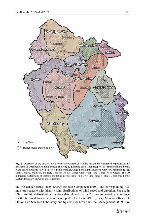
Fig. 6 Map of pixel-level mean fireline intensity across the BDNF fire modeling landscape. Mean firelineintensity values range from a high near 56,000 kW/m in intact forested areas to a minimum near 200 kW/m.Black indicates non-burnable areas of the landscape (primarily agricultural land)

Nat Hazards (2012) 64:707–728 719

123

Fig. 7 Map of integrated wildfire hazard across the BDNF fire modeling landscape. Integrated wildfirehazard is the product of BP and MFI. Values of integrated wildfire hazard span nearly six orders ofmagnitude. The values are highest in the still-intact, crown fire-capable forests of the high BP NW region ofthe landscape, and lowest in the forests, now prone to low-intensity surface fire and low-grade passive crownfire due to defoliation by beetles, found in the low-probability band trending from the SW to the NE corner

720 Nat Hazards (2012) 64:707–728

123

Fig. 8 Box plots of BP, MFI, and integrated hazard for all 10 municipal watersheds, sorted by meanintegrated hazard. Box plots indicate the quartiles (the box), 10th/90th percentiles (whiskers), median (blackline), mean (thick gray line), and individual values outside the 10th/90th percentiles (dots)

Nat Hazards (2012) 64:707–728 721

123

3 Results

Wildfire hazard characteristics vary considerably across the analysis area. The regions of

the landscape with the highest annual burn probabilities—the northwest and southeast

portions of the landscape (Fig. 5)—exhibit BP values in the range from 0.003 to 0.010.

These areas correspond to the regions with the highest ignition density (see Fig. 3). Burn

probabilities are lowest in the southwest–northeast band that corresponds to low ignition

density. Burn probability in this area ranges broadly from 0.0002 to 0.0010. The range of

simulated burn probability values encompasses the non-spatial, historical average annual

burn probability of 0.0012.

Fig. 9 Wildfire hazardcharacteristics chart for twocontrasting municipalwatersheds. Gray dots indicatewatershed J (watershed with thelowest integrated hazard); blackdots indicate watershed D(highest integrated hazard)

Table 2 Summary of pixel-based wildfire hazard characteristics within each of the ten municipal water-sheds on the Beaverhead-Deerlodge National Forest

(a)Watershed

Mean of burnable pixels (e)Expected annual area

burned (ha/year)(b)Burn

probability

(c)Mean fireline

intensity (kW/m)

(d)Integrated wildfire hazard

(kW/(m-year))

A 0.0001628 1,014 0.2098 1.64

B 0.0001634 409 0.0730 0.51

C 0.0004873 1,827 0.8996 0.25

D 0.0013794 3,952 5.8270 1.00

E 0.0009767 2,980 2.9960 2.44

F 0.0004720 1,142 0.6248 2.80

G 0.0008151 3,858 3.3200 1.29

H 0.0002570 593 0.2298 0.32

I 0.0009899 3,103 3.1151 1.29

J 0.0001347 463 0.0633 0.18

Expected annual area burned (column e) is the product of watershed-mean burn probability (column b) andthe burnable watershed area (Table 1, column d). Expected annual area burned as a fraction of the burnablewatershed area is therefore equivalent to the watershed-mean burn probability

722 Nat Hazards (2012) 64:707–728

123

Forested areas less impacted by the beetles at the time of the analysis, like the Clark

Fork-Flints landscape, exhibit higher MFI values than those heavily impacted, such as the

Boulder River landscape, where the highest MFI values reach just half that amount

(Fig. 6). Valley-bottom grasslands exhibit moderate MFI values relative to much of the

beetle-impacted forests, but the intact forests produce the highest MFI values in the fire

modeling area. Low MFI values can exist adjacent to areas with high MFI values because

of localized fuelbed characteristics. Lastly, the areas of greatest integrated hazard occur

where both BP and MFI are high—the still-dense forests of the northwest and southeast

corners of the analysis area—where watersheds D, E, G, and I are located (Fig. 7).

Box plots depicting the distribution of BP, MFI, and integrated hazard within each

watershed illustrate a large range of variability of wildfire hazard (Fig. 8). Within any

given watershed, MFI varies across roughly four orders of magnitude, despite the fact that

MFI is itself a pixel mean that masks some variability. Fireline intensity inherently ranges

across roughly five orders of magnitude, from a low of 10 kW/m for a backing fire in light

fuel to a high of 100,000 kW/m for a fast-spreading crown fire. Burn probability varies

across 1–2 orders of magnitude within a watershed. Generally speaking, larger watersheds

exhibit greater variability in BP. Because integrated hazard is the product of BP and MFI,

and because BP and MFI vary so greatly themselves, integrated hazard varies across 4–5

orders of magnitude. Integrated wildfire hazard is sorted into classes, indexed by roman

numerals and partitioned according to the orders of magnitude. Median watershed hazard

class values range from class III to class VI, with four watersheds in the highest observed

hazard class (D, E, G, and I). Watersheds A, B, and J appear to have the least exposure to

wildfire. The variability of integrated hazard within watersheds appears to be largely driven

by variation in mean fireline intensity, whereas variation between watersheds appears to be

driven largely by burn probability.

The joint distribution of BP and MFI for two contrasting watersheds is depicted in a

wildfire hazard characteristics chart (Fig. 9). Watershed J is the watershed with the lowest

mean integrated hazard, whereas watershed D has the highest hazard. As seen on this chart

and in Fig. 8, their BP values differ by a factor of ten. In contrast, they exhibit a similar

overall range of MFI values. Watershed D, however, has a higher concentration of pixels in

the upper range of the MFI scale, resulting in a much higher watershed-mean MFI. Fig-

ure 9 reveals a bimodal distribution of MFI within watershed D that is not apparent in the

box plots, with one cluster of points in the 1,000 to 10,000 kW/m range and another

clustered around 10 kW/m. This bimodal distribution is largely a function of the under-

lying fuelbed. The lower cluster of points is simply not capable of producing high fireline

intensity values—it consists of compact forest litter and is found on the lee side of a small

lake, causing many fires to flank through this area rather than spread through as a heading

fire. The cluster of higher MFI values consists of fuels characterized by litter with a grass

component and a forest canopy capable of supporting passive and active crown fire.

Watershed-mean BP values are likewise highly variable (Table 2; column b), varying

by an order of magnitude between the highest (watershed D; 0.0013794) and lowest

(watershed J; 0.0001347). The non-spatial average annual historical BP is on the higher

end with respect to mean watershed BP, suggesting that municipal watersheds are largely

located in areas of lower fire hazard relative to the broader landscape. Relative ignition

density exhibits fairly high positive correlations with both BP (0.70) and MFI (0.85),

highlighting the potential influence of modeled ignition processes on modeled fire growth

and behavior.

Mean fireline intensity is similarly variable (Table 2; column c), ranging from a high of

3,952 kW/m in watershed D to a low of 409 kW/m in watershed B. Watershed D has the

Nat Hazards (2012) 64:707–728 723

123

highest mean integrated wildfire hazard (Table 2; column d), which is not surprising given

it ranks highest in both components of integrated hazard (burn probability and fireline

intensity). Watershed J, by contrast, has the lowest mean integrated hazard, ranking last in

burn probability and second to last in mean fireline intensity. Lastly, watershed F has the

highest expected value of annual area burned (Table 2; column e), a function of moderate

burn probability (6th highest) and relatively large burnable area (second highest). Expected

area burned as a fraction of the watershed size is equivalent to the watershed-mean BP

(Table 2, column b).

4 Discussion

The research effort presented here illustrates the application of geospatial analysis, large-

fire simulation, and burn probability modeling to examine pixel-based measures of wildfire

hazard and watershed exposure. The derivation of an integrated measure of wildfire hazard

(product of BP and MFI) provides a useful filter for identifying watersheds that are par-

ticularly likely to burn with high intensity and for informing mitigation and prioritization

efforts. Thus, a multitude of wildfire hazard and exposure characterizations exist and can

jointly inform wildfire risk analyses.

A logical next step would be to analyze potential wildfire consequences to municipal

watersheds and post-fire impacts to water quality. Additional spatial variables relevant to

watershed health or susceptibility, such as slope steepness and erosive potential could be

incorporated into our integrated wildfire hazard index. Associating fireline intensity with

primary vegetation type to predict fire severity would improve projection of fire effects;

strong erosion response is not necessarily always associated with high flame lengths,

especially for herbaceous fuels (Parsons et al. 2010). Rather, post-fire hydrogeomorphic

response is strongly correlated with spatial extent and distribution of moderate and high

burn severity (Cannon et al. 2010; Gartner et al. 2008; Hyde et al. 2007). Thus, coupling

our modeling approach with burn severity models could be particularly informative. We

could then further couple estimates of post-fire vegetation removal with slope stability

models to estimate changes to landslide susceptibility (Ren et al. 2011).

There are a number of challenges associated with fire effects prediction that could be

identified and addressed in future expansions. Estimating resource response to fire can be

confounded by complex spatiotemporal dynamics and limited scientific understanding

(Keane et al. 2008). Existing models provide useful information on likely first-order fire

effects, but some level of inference is still necessary to characterize second-order fire

effects (e.g., impacts to water quality) that often are of greater interest to managers

(Reinhardt and Dickinson 2010). Approaches adopted in the literature include pairing fire

outputs with secondary simulation or process-based models and reliance on expert judg-

ment (Thompson et al. 2011b; Keane and Karau 2010; Ager et al. 2007; Roloff et al. 2005).

Embedding additional ecological models may come with costs of increased data demands

and propagated uncertainty.

It is important to explicitly recognize modeling assumptions and their potential influ-

ence on results. In our case, there are at least two major assumptions to highlight. First, due

to a lack of a locally available high-resolution ignition density grid, we assumed a coarser

national-scale grid would be sufficient. A comparison of recent ignitions and grid density

values (Fig. 3) suggests our assumption is valid, but this may not always be the case. The

influence of modeled ignitions on burn probabilities can be substantial, as our results

comparing relative ignition density and wildfire hazard characteristics indicated, and

724 Nat Hazards (2012) 64:707–728

123

further as indicated in recent studies (Parks et al. 2012; Bar Massada et al. 2011). Second,

our modeling of the impacts of the beetle infestation on fuel conditions likely influenced

results. We modeled the longer-duration gray phase and assumed reduced canopy bulk

density and canopy cover, which tended to reduce crown fire potential and mean fireline

intensity in affected areas. If fires occur in the near-term red phase, we might expect

significantly different fire behavior. The specific impacts of beetles on fuel conditions and

fire behavior are an ongoing debate within the fire modeling community (e.g., Moran and

Cochrane 2012; Jolly et al. 2012; Simard et al. 2012).

There is also a need to consider the limitations and uncertainties of fire modeling tools.

Sullivan (2009a, b, c) offers a comprehensive overview of surface fire spread modeling,

highlighting a need to improve basic fire science and to better understand how uncertainty

and errors propagate through models. Assumptions and prediction errors related to crown

fire potential and propagation, and limited consideration of dynamic fire–atmosphere and

fire–fuels interactions are of particular concern (Ager et al. 2011; Cruz and Alexander

2010; Mell et al. 2010). Thus, caution in scope of inference and careful data critiquing and

validation is warranted. Output from wildfire simulation models is one the component of a

broader set of information used to guide mitigation and restoration planning and can be

viewed as a complement to local expertise. With respect to our application, we devoted

considerable energy to acquiring, critiquing, and editing geospatial fuels data with atten-

tion to guidance (Stratton 2009) and with the assistance of BDNF fire and fuel management

staff. FSim has undergone validation efforts at the national scale (Finney et al. 2011), and

our modeling results across the landscape studied here indicate agreement with a (limited)

historical fire record.

Burn probability modeling is increasingly used across the fire and fuels management

continuum. The analytical work presented in this article could inform pre-season planning

and fire management plan updating, and in particular has application to fuel management

planning. Landscape-scale fuel treatment planning combines risk-based analyses of fuel

management needs with identification of feasible management opportunities. Treatment

strategy design could seek to interrupt major fire flow paths to reduce likelihood of spread

into susceptible watersheds and/or to mitigate fire behavior and burn severity within

watersheds. A process of comparative risk assessment could evaluate and rank alternative

hazardous fuels reduction strategies in terms of impacts to wildfire hazard and exposure.

Prioritizing treatments could additionally be based on relative importance weights assigned

to municipal watersheds based upon quantity, demographics, and socioeconomic vulner-

ability (e.g., Gaither et al. 2011) of population served.

5 Conclusion

This research effort presents novel approaches to characterize wildfire hazard and thereby

advances the science of wildfire exposure analysis and risk assessment. Our wildfire hazard

and exposure assessment sought to understand where and under what conditions fire is

likely to interact with municipal watersheds. Combining spatially explicit information on

burn probability and fireline intensity provides useful information for prioritizing mitiga-

tion and restoration efforts. The derivation of pixel-based integrated hazard metrics

improves our ability to consider the potential ecological and human health impacts asso-

ciated with wildfire on the landscape. As our ability to understand and model fire effects

improves so too will our ability to integrate wildfire hazard analyses into more informative

risk analyses that focus on estimating both likelihood and consequences of wildfire.

Nat Hazards (2012) 64:707–728 725

123

In our case study of wildfire hazard and exposure on the Beaverhead-Deerlodge

National Forest, we developed novel classification systems for wildfire hazard and expo-

sure, and used this system to highlight threatened municipal watersheds. We demonstrated

vast differences in fire likelihood, fire behavior, and expected area burned across municipal

watersheds. Given the high priority on protecting human life and safety and the subsequent

obligation to protect drinking water from wildfire-related degradation, the nature of

analysis we present here could have wide application across the nation.

Acknowledgments We would like to thank the staff of the Beaverhead-Deerlodge National Forest, andKevin Hyde, Tyron Venn, and two anonymous reviewers. The Rocky Mountain Research Station andNational Fire Decision Support Center supported this effort.

References

Agee JK (1993) Fire ecology in the Pacific Northwest forests. Island Press, WashingtonAger AA, Finney MA, Kerns BK, Maffei H (2007) Modeling wildfire risk to northern spotted owl (Strix-

occidentaliscaurina) habitat in Central Oregon, USA. For Ecol Manag 246(1):45–56Ager AA, Valliant NM, Finney MA (2010) A comparison of landscape fuel treatment strategies to mitigate

wildland fire risk in the urban interface to preserve old forest structure. For Ecol Manag 259(8):1556–1570

Ager AA, Vaillant NM, Finney MA (2011) Integrating fire behavior models and geospatial analysis forwildland fire risk assessment and fuel management planning. J Combust. Article ID 572452, p 19. doi:10.1155/2011/572452

Ahl R, Weldon H, Vanderzanden D (2010) Rapid response VMPA production for the Beaverhead-Deer-lodge national forest with an application of the Random Forest classification algorithm. Version 10.1.USDA Forest Service, Northern Region Engineering Geospatial Services Group, May 2010 (unpub-lished report) Missoula, MT

Bar Massada A, Radeloff VC, Stewart SI, Hawbaker TJ (2009) Wildfire risk in the wildland-urban interface:a simulation study in northwestern Wisconsin. For Ecol Manag 258:1990–1999

Bar Massada A, Radeloff VC, Stewart SI (2011) Allocating fuel breaks to optimally protect structures in thewildland-urban interface. Int J Wildland Fire 20:59–68

Benda LE, Miller D, Bigelow P, Andras K (2003) Effects of post-wildfire erosion on channel environments,Boise River, Idaho. For Ecol Manag 178:105–119

Bisson PA, Rieman BE, Luce CH, Hessburg PF, Lee DC, Kershner JL, Reeves GH, Gresswell RE (2003)Fire and aquatic ecosystems of the western USA: current knowledge and key questions. For EcolManag 178:213–229

Brauman KA, Daily GC, Ka’eo Duarte T, Mooney HA (2007) The nature and value of ecosystem services:an overview highlighting hydrological services. Annu Rev Environ Resour 32:67–98

Brown TC (2000) Economic issues for watersheds supplying drinking water. In: Dissmeyer GF (eds)Drinking water from forests and grasslands: a synthesis of the scientific literature. USDA ForestService GTR SRS-39. Southern Research Station, Asheville, North Carolina, pp 42–54. Online:http://www.srs.fs.usda.gov/pubs/gtr/gtr_srs039/gtr_srs039.pdf. Accessed August 19, 2010

Brown TC, Binkley D (1994) Effect of management on water quality in North American forests. GeneralTechnical Report GTR RM-248. USDA Forest Service Rocky Mountain Forest and Range ExperimentStation. Fort Collins, CO

Brown TC, Froemke P (2010) Risk of impaired condition of watersheds containing national forest lands.General Technical Report RMRS-GTR-251. USDA Forest Service Rocky Mountain Research Station,Fort Collins, CO, p 57

Brown TC, Hobbins MT, Ramirez JA (2008) Spatial distribution of water supply in the coterminous UnitedStates. J Am Water Res As 44(6):1474–1487

Calkin DE, Hyde KD, Robichaud PR, Jones JG, Ashmun LE, Loeffler D (2007) Assessing post-fire values-at-risk with a new calculation tool. General Technical Report RMRS-GTR-205. USDA Forest Service,Rocky Mountain Research Station, Fort Collins, CO

Calkin DE, Ager AA, Thompson MP (2011a) A comparative risk assessment framework for wildland firemanagement: the 2010 cohesive strategy science report. General Technical Report RMRS-GTR-262.US Department of Agriculture, Forest Service, Rocky Mountain Research Station, Fort Collins, p 63

726 Nat Hazards (2012) 64:707–728

123

Calkin DE, Thompson MP, Finney MA, Hyde KD (2011b) A real-time risk-assessment tool supportingwildland fire decision-making. J For 109(5):274–280

Cannon SH, Gartner JE, Rupert MG, Michael JA, Rea AH, Parrett C (2010) Predicting the probability andvolume of post wildfire debris flows in the intermountain western United States. GSA Bull 127–144.doi:10.1130/B26459.1.122

Cruz MG, Alexander ME (2010) Assessing crown fire potential in coniferous forests of western NorthAmerica: a critique of current approaches and recent simulation studies. Int J Wildland Fire19(4):377–398

Dennison PE, Cova TJ, Mortiz MA (2007) WUIVAC: a wildland-urban interface evacuation trigger modelapplied in strategic wildfire scenarios. Nat Hazards 41:181–199

Dunham JB, Rosenberger AE, Luce CH, Rieman BE (2007) Influences of wildfire and channel reorgani-zation on spatial and temporal variation in stream temperature and the distribution of fish andamphibians. Ecosystems 10:335–346

Emelko MB, Silins U, Bladon KD, Stone M (2011) Implications of land disturbance on drinking watertreatability in a changing climate: demonstrating the need for ‘source water supply and protection’strategies. Water Res 45:461–472

Fairbrother A, Turnley JG (2005) Predicting risks of uncharacteristic wildfires: application of the riskassessment process. For Ecol Manag 211:28–35

Finney MA (1998) FARSITE: fire area simulator—model development and evaluation. USDA ForestService, Research Paper RMRS-RP-4, p 47

Finney MA (2002) Fire growth using minimum travel time methods. Can J For Res 32(8):1420–1424Finney MA (2005) The challenge of quantitative risk assessment for wildland fire. For Ecol Manag

211:97–108Finney MA, Grenfell IC, McHugh CW (2009) Modeling containment of large wildfires using generalized

linear mixed-model analysis. Forest Sci 55(3):249–255Finney MA, McHugh CW, Stratton RD, Riley KL (2011) A simulation of probabilistic wildfire risk

components for the continental United States. Stoch Environ Res Risk Assess. doi:10.1007/s00477-011-0462-z

Fire Executive Council (2009) Guidance for implementation of federal wildland fire management policy. 13Feb 2009. Available at: http://www/nifc/gov/policies/guidance/GIFWFMP.pdf

Gaither CJ, Poudyal NC, Goodrick S, Bowker JM, Malone S, Gan J (2011) Wildland fire risk and socialvulnerability in the Southeastern United States: an exploratory spatial data analysis approach. ForPolicy Econ 13:24–36

Gartner JE, Cannon SH, Santi PM, Dewolfe VG (2008) Empirical models to predict the volumes of debrisflows generated by recently burned basins in the Western US. Geomorphology 96:339–354

Hyde K, Woods SW, Donahue J (2007) Predicting gully rejuvenation after wildfire using remotely sensedburn severity data. Geomorphology 86:496–511

Jenkins MJ, Hebertson E, Page WG, Jorgensen CA (2008) Bark beetles, fuels, fires and implications forforest management in the intermountain West. For Ecol Manag 254:16–34

Jolly WM, Parsons R, Varner JM, Butler BW, Ryan KC, Gucker CL (2012) Do mountain pine beetleoutbreaks change the probability of active crown fire in lodgepole pine forests? Comment Ecol93(4):941–946

Keane R, Karau E (2010) Evaluating the ecological benefits of wildfire by integrating fire and ecosystemsimulation models. Ecol Model 221:1162–1172

Keane RE, Agee JK, Fule P, Keeley JE, Key C, Kitchen SG, Miller R, Schulte LA (2008) Ecological effectsof large fires on US landscapes: benefit or catastrophe? Int J Wildland Fire 17:696–712

LANDFIRE (2010) Homepage of the LANDFIRE Project, US Department of Agriculture, Forest Service;US Department of Interior, [Online]. Available: http://www.landfire.gov, 10 Dec 2010

Mell WE, Manzello SL, Maranghides A, Butry D, Rehm RG (2010) The wildland-urban interface fireproblem: current approaches and 214 research needs. Int J Wildland Fire 19:238–251

Miller C, Parisien MA, Ager AA, Finney MA (2008) Evaluating spatially explicit burn probabilities forstrategic fire management planning. Trans Ecol Environ 19:245–252

Monitoring Trends in Burn Severity (MTBS) (2010) Homepage of the MTBS multi-year project, USGeological Survey National Center for Earth Resources Observation and Science (EROS); USDAForest Service Remote Sensing Applications Center (RSAC), [Online]. Available: http://www.mtbs.gov/index.html. Last Update October 2010

Moody JA, Martin DA (2009) Synthesis of sediment yields after wildland fire in different rainfall regimes inthe western United States. Int J Wildland Fire 18:96–115

Moran CJ, Cochrane MA (2012) Do mountain pine beetle outbreaks change the probability of active crownfire in lodgepole pine forests? Comment Ecol 93(4):939–941

Nat Hazards (2012) 64:707–728 727

123

Neary DG, Ryan KC, DeBano LF (eds) (2005) Wildland fire in ecosystems: effects of fire on soils and water.Gen. Tech. Rep. RMRS-GTR-42-vol 4. USDA Forest Service, Rocky Mountain Research Station,Ogden, UT, p 250

Noonan-Wright EK, Opperman TS, Finney MA, Zimmerman GT, Seli RC, Elenz LM, Calkin DE, FiedlerJR (2011) Developing the US wildland fire decision support system. J Combust. Article ID 168473,p 14. doi:10.1155/2011/168473

Page WG, Jenkins MJ (2007a) Mountain pine beetle-induced changes to selected lodgepole pine fuelcomplexes within the intermountain region. Forensic Sci 53:507–518

Page WG, Jenkins MJ (2007b) Predicted fire behavior in selected mountain pine beetle-infested lodgepolepine. Forensic Sci 53:662–674

Parise M, Cannon SH (2012) Wildfire impacts on the processes that generate debris flows in burnedwatersheds. Nat Hazard. doi:10.1007/s11069-011-9769-9

Parks SA, Parisien MA, Miller C (2012) Spatial bottom-up controls on fire likelihood vary across westernNorth America. Ecosphere 3(1):20. Article 12

Parsons A, Robichaud PR, Lewis SA, Napper C, Clark JT (2010) Field guide for mapping post-fire soil burnseverity. USDA Forest Service, Rocky Mountain Research Station, RMRS-GTR-243, Fort Collins, CO

Reeves MC, Ryan KC, Rollins MG, Thompson TG (2009) Spatial fuel data products of the LANDFIREproject. Int J Wildland Fire 18:250–267

Reinhardt ED, Dickinson MB (2010) First-order fire effects models for land management: overview andissues. Fire Ecol 6(1):131–142

Ren D, Fu R, Leslie LM, Dickinson RE (2011) Modeling the mudslide aftermath of the 2007 SouthernCalifornia Wildfires. Nat Hazards 57:327–343

Rieman BE, Hessburg PF, Luce C, Dare MR (2010) Wildfire and management of forests and native fishes:conflict or opportunity for convergent solutions? Bioscience 60(6):460–468

Rocky Mountain Research Station Fire Sciences Laboratory and Systems for Environmental Management(2002) FireFamilyPlus user’s guide, version 3.0. US Department of Agriculture, Forest Service,National Fire and Aviation Management Information Systems Team, Boise

Roloff GJ, Mealey SP, Clay C, Barry J, Yanish C, Neuenschwander L (2005) A process for modeling short-and long-term risk the southern Oregon Cascades. For Ecol Manag 211:166–190

Ryan D, Samuels WB (2010) Fire vs. water: a new tool assesses drinking water’s risk from wildland fires.Geoworld 23(7):16–20

Shakesby RA, Doerr SH (2006) Wildfire as a hydrological and geomorphological agent. Earth-Sci Rev74:269–307

Sikder IU, Mal-Sarkar S, Mal TK (2006) Knowledge-based risk assessment under uncertainty for speciesinvasion. Risk Anal 26(1):239–252

Simard M, Romme WH, Griffin JM, Turner MG (2011) Do mountain pine beetle outbreaks change theprobability of active crown fire in lodgepole pine forests. Ecol Mongr 81(1):3–24

Simard M, Romme WH, Griffin JM, Turner MG (2012) Do mountain pine beetle outbreaks change theprobability of active crown fire in lodgepole pine forests? Reply Ecol 93(4):946–950

Smith HG, Sheridan GJ, Lane PNJ, Nyman P, Haydon S (2010) Wildfire effects on water quality in forestcatchments: a review with implications for water supply. J Hydrol 396:170–192

Stratton RD (2009) Guidebook on LANDFIRE fuels data acquisition, critique, modification, maintenance,and model calibration. Gen. Tech. Rep. RMRS-GTR-220. US Department of Agriculture, ForestService, Rocky Mountain Research Station, Fort Collins, p 54

Sullivan AL (2009a) Wildland surface fire spread modelling, 1990–2007. 1: physical and quasi-physicalmodels. Int J Wildland Fire 18:349–368

Sullivan AL (2009b) Wildland surface fire spread modelling, 1990–2007. 2: empirical and quasi-empiricalmodels. Int J Wildland Fire 18:369–386

Sullivan AL (2009c) Wildland surface fire spread modelling, 1990–2007. 3: simulation and mathematicalanalogue models. Int J Wildland Fire 18:387–403

Thompson MP, Calkin DE (2011) Uncertainty and risk in wildland fire management: a review. J EnvironManag 92:1895–1909

Thompson MP, Calkin DE, Finney MA, Ager AA, Gilbertson-Day JW (2011a) Integrated national-scaleassessment of wildfire risk to human and ecological values. Stoch Environ Res Risk Assess25(6):761–780

Thompson MP, Calkin DE, Gilbertson-Day J, Ager AA (2011b) Advancing effects analysis for integrated,large-scale wildfire risk assessment. Environ Monit Assess 179(1–4):217–239

728 Nat Hazards (2012) 64:707–728

123