Contents lists available at SciVerse ScienceDirect
Electric Power Systems Research
jou rn al h om epa ge: www.elsev ier .com/ locate /epsr
robabilistic assessment of wind farm annual energy production
uhammad Alia, Julija Matevosyanb, J.V. Milanovic a,∗
The University of Manchester, School of Electrical and Electronic Engineering, Sackville Street, Manchester M13 9PL, UKSinclair, Knight & Merz, Level 7, Victoria House, Southampton Row, London WC1B 4EA, UK
r t i c l e i n f o
rticle history:eceived 26 July 2011eceived in revised form9 November 2011ccepted 29 January 2012vailable online 29 March 2012
a b s t r a c t
Energy yield (EY) evaluation of a wind farm (WF) is essential for profit estimation and such analysis isusually part of the pre-feasibility study for any WF. Energy output from a WF can vary because of severalfactors including site location and WF layout. It is therefore essential to estimate EY accurately takinginto account as many realistic effects as possible. Both energy output from a WF as well as transfer ofenergy into the grid are vital information. In this paper, methodologies are provided to calculate losses
eywords:ind power generation
ower transmissionind energy
eliability
due to wake effect, internal WF collector system, and a new method to calculate unavailability of windturbine (WT) and WF components. A novel method to calculate wind energy curtailments due to networktransmission bottlenecks is also presented considering internal WF losses for four collector systems.Correlations between incoming wind speed (WS), WT availability and Transmission Line Loading (TLL)are used to determine range of wind energy curtailments for several possible scenarios. Impact of windresource variation (at a site) on energy output and energy curtailed is also analysed.
. Introduction
Energy output is the main factor that contributes towards feasi-ility of a wind project. A reasonably realistic estimate can only bebtained once all important factors have been taken into account,uch as availability of wind resource from a site, wake effect within
WF, electrical power losses in a WF collector system, WT and cablevailability in a WF collector system as well as energy losses due toind energy curtailments.
A general method to estimate the amount of EY is by usingeibull distribution (if site measurements are not available), tur-
ine power curves and number of WTs inside a WF. Normally, once rough EY estimate is obtained then electrical losses and wakeosses are subtracted as a fixed number [1]. For example [1,2] used
Abbreviations: EY, energy yield; WF, wind farm; WT, wind turbine; WS, windpeed; WD, wind direction; TLL, Transmission Line Loading; WPPDF, Wind Powerroduction Distribution Function; WP, wind power; ADF, Availability Density Func-ion; PCC, Point of Common Coupling; WPDC, Wind Production Duration Curve;DC, Availability Duration Curve; WPDC′ , New Wind Production Duration Curve;DC, Unavailability Distribution Curve; TDC, Transmission Duration Curve; C, Lineapacity; TDF, Transmission Probability Distribution Function; WDF, Wind farmroduction Probability Distribution Function; NTDF, New Transmission Probabil-ty Distribution Function; TL, Transmission Limit; XLPE, cross-linked polyethylene;orr., correlation; p.u., per unit; Max., maximum; Min., minimum; Comp., compo-ent.∗ Corresponding author. Tel.: +44 161 306 8724.
this method to estimate the value of overall EY from a WF. In reality,doing so would lead to inaccurate estimation because these calcu-lations are case specific and vary significantly with size and layoutof the WF. They also depend on the choice of electrical equipmentand electrical connection strategy internal to the WF. Along with agood estimation of EY (considering all influencing factors) it is alsobeneficial to determine the amount of energy that can be trans-ferred into the network. For instance, if a WF is connected to a partof network where transmission capacity of lines cannot carry allof WF power produced during the entire year. A complete proba-bilistic analysis would enable the WF owner to know the amountof energy likely to be produced and transferred into the grid whichtranslates into profits.
In spite of the fact that there exist some commercial packagesfor EY estimation, the methods and procedures applied there arenot reported and it is difficult to see how different parameters andeffects are accounted for. This paper, in addition to addressing theeffects included in commercial packages, provides detailed descrip-tion of the methodologies used to model those effects, and proposesnew methods to: (i) account for losses due to unavailability of WTsand cables within a WF for four collector systems; (ii) estimatepossible wind energy curtailments in networks with transmissionbottlenecks using correlations between WS, WT availability and TLLconsidering wakes and electrical losses as well as WF componentavailability. Impact of wind resource variation on energy produced
and energy curtailed is also investigated. A sensitivity analysis isfinally performed to assess how much different parameters affectestimated EY in order to establish their significance for this type ofstudies.
Wind potential is dependent on ambient and terrain conditionst a site. In order to evaluate wind potential, WS is measured fort least 1 year. However longer measured periods are better sinceind potential vary by about 10% from year to year [3]. Wind
urbine generates power only if the incoming WS is between itsperating range, i.e. between cut-in and cut-out speed. Power pro-uction of WT is then calculated using:
WT (v) = 0.5cp(v)A�v3 (1)
here A is a swept area of the WT rotor, � is air density and cp(v)s overall efficiency of WT at wind speed v. Once WS distributions known, Wind Power Production Distribution Function (WPPDF)an be calculated. For simplicity, let Y be expected wind power (WP)roduction in MW. Using WS distribution function, the power pro-uction state Y of the planned WF can be obtained multiplying (1)y a number of WTs K in a WF.
Then discrete probability density and distribution functions of are calculated as follows:
Y (y) = P(Y = y) = hY (y)N
; FY (y) = P(Y ≤ y) =∑i:yi≤y
fY (yi) (2)
here P(Y = y) is the probability that WP production Y is equal to a(MW), hY(y) is frequency of y, N is number of WS measurements.inally, EY of a WF is calculated:
=ymax∑y=0
FY (y) · �y (3)
here �y is a step at which wind production probability distribu-ion function FY(y) is discretised. This method to obtain an initialstimate of EY was used in [1,2]. The following section provides theethod to calculate wake losses analytically by calculating WS at
ach WT inside the WF and then power; this is a more accuratepproach.
.2. Wake effects
When wind strikes the rotor of a WT some of the wind energy isonverted into mechanical and then electrical energy whereas theest remains unconverted and is reduced in speed and becomesurbulent. It is referred to as a wake. A downstream turbine receiv-ng this slow and turbulent wind will produce less electricity ands exposed to greater mechanical stress. The WS behind a turbines calculated as [4,5]:
1 = u
[1 −(
ro
ro + cxo
)2(1 −
√1 − Ct)
](4)
here c is the decay constant which represents the effects of atmo-pheric stability, ro is the radius of the WT, u is the speed ofree-stream wind received by the turbine with the thrust coeffi-ient, Ct, and v1 is the WS at a distance xo from a WT. If a WT isartially shaded (ps) the WS at rotor disc of interest is determinedy calculating the ratio (weighting factor, ˇ) between the rotor area
n wake and the total rotor area. WS into the WT is then [6]:
tj = u
(1 −√∑
ˇTj,Th
(1 − vps,Th
u
)2)
(5)
h
here j is the WT under wake, h is the upwind turbine, u is the initialS entering into the WT h, vps,Th is the shadow of WT h falling onT j. In a large WF, several WTs may be arranged one behind the
Fig. 1. Wind speed at turbines calculated using wake model, incoming WS = 10 m/s.
other. Turbines downwind in the same column receive less winddue to two or more upwind turbines. This effect is called multiplewakes and WS approaching, e.g., the third turbine in a column iscalculated using [7]:
v2 = u
[(ro
ro + cxo
)2((
v1
√1 − Ct
u
)− 1
)+ 1
](6)
Wake effects in this study are modelled using detailed modelsconsidering single, partial and multiple shadowing of WTs. Theresults obtained by these formulae for a wind farm with two dif-ferent turbine distances, 5D and 7D, are plotted in Fig. 1, where Dis the rotor diameter of a turbine in meters. The results of calcula-tion have been validated against actual wind speed data measuredinside a wind farm given in [8,9,10]. Applying wake effect model toWS measurements from the site, the WS at each WT within a WFcan be estimated for a given WF layout. Since wake effect dependson both, speed and direction of the incoming wind, the power pro-duction of each WT is calculated after modelling wakes for everyincoming WS and WD. Total EY of the WF can then be estimatedsumming individual WT productions for the whole year. There aremany site specific factors which influence wake effect and hencethe EY. These include wind characteristics of a site, air density, sizeand layout of the WF, height of the WT, distance between the tur-bines, WF location, radius of the WT rotor, thrust coefficient curveand power curve of the WT. Impact of some of these factors onEY are briefly discussed below. Wake effects are considered foronshore and offshore WFs with standard terrain roughness lengthsof 0.0002 m and 0.1 m respectively [11]. The value of decay con-stant c depends on site location, it is usually set to 0.075 for onshoreand 0.04 for offshore sites [12]. Highest wake losses typically occurfor WS between 6 and 10 m/s [8] when thrust coefficient Ct is high,however, this is also dependant on the wind direction (WD). Thrustcoefficient determines total momentum deficit in the wake of a WT.Both thrust coefficient and power coefficient are linked to axialinduction factor a [13] which is linked with rotor radius and wakeradius downstream [14]:
Cp = 4a(1 − a)2 (7)
Ct = 4a(1 − a) (8)
rw = r0
√1 − a
1 − 2a(9)
Thrust coefficient dependence on WS curves (C curves) is differ-
t
ent for different makes of WT, i.e., different WT manufacturers andit should be (ideally) provided by the WT manufacturers. As gen-eral estimate of the thrust coefficient however, the formula (10)
72 M. Ali et al. / Electric Power Systems Research 89 (2012) 70– 79
da
C
2
lcesrF
P
wpiam
P
P
Fdcfrsecampcct
Fig. 3. Central collector system.
Fig. 2. Radial collector system.
erived in [15] can be used. (This formula was validated in [16]fter comparing Ct curves for several WTs.)
t = 3.5(2u − 3.5)u2
≈ 7u
m/s (10)
.3. Electrical power losses
EY from a WF is further reduced due to electrical losses in the col-ector system. These losses vary with the type of collector system,able parameters and transformers used. Four typical (used in thexisting WFs or most commonly discussed in literature) collectorystems configurations are considered: Radial, Star, Single-sideding and Central collector systems. In a Radial collector system,ig. 2, the electrical power loss in a string can be found as [5]:
here R is line resistance, I is the current flowing in the lines. Onceower loss from each string is evaluated, the total power losses
n the WF can be found as a sum of power loss in m strings [5]long with power loss in the main cable carrying current from all
strings to the shore.
cable to shoreloss = 3
⎡⎣R1
(m∑1
Ii
)2⎤⎦ (12)
totalloss =
[m∑1
Pstringloss
]+ Pcable to shore
loss (13)
or Central collector system configuration, Fig. 3 (e.g. used for Mid-elgrunden WF [17]), the power losses can be calculated as in Radialonfiguration with only two strings using (11)–(13). The currentrom two strings is collected at one central WT. For Single-sideding system, Fig. 4, the power loss is computed for each stringimilar to that of Radial configuration (11) however in this caseach string is carrying power directly to the shore therefore mainable from last turbine to shore has higher impedance. Total lossesre equal to sum of losses in the individual strings. Each stringight be equipped with a redundant line capable of transferring
ower in case of a fault in the main cable. The increased securityomes however at extra cost for redundant lines. The power lossalculation for Star collector system, Fig. 5, is slightly different fromhe above. There are different ways to set-up a star network [17,18].
Fig. 5. Star collec
Fig. 4. Single-sided ring collector system.
The configuration analysed here is based on [18] and illustrated inFig. 5. The total power loss is defined by (14)–(17) for m clusters.
Ptotal starloss = 3[R1I2
1 + R2I22 + · · · + R7I2
7] + P8 + P9 (14)
P8 = 3[(I8 + I7 + I6 + · · · + I1)2R8] (15)
P9 = 3[(I9 + I8 + I7 + · · · + I1)2R9] (16)
Ptotalloss =
m∑i=1
Ptotal starloss (17)
In general, losses inside transformers are divided into two types,no-load losses and load losses. No-losses arise due to energisationof the core of the transformer and remain unaffected by the load-ing of the transformer. Load losses vary depending on the amountof power transferred through the windings (copper losses). Loadlosses are simply I2R losses and can increase as the amount of cur-rent increases through the winding coils. Therefore if current andresistance of the winding coils are known they can be easily com-puted. No-load losses on the other hand remain constant; and aregenerally a small percentage of the MVA of a transformer.
2.4. Wind farm losses due to reliability considerations
With development of WT technology and increase of WF size,reliability is becoming more and more important as it can influ-ence energy delivered. Analysis of reliability indices of differentWT components based on cumulative statistics is given in [19]. Ref.[20] is providing more detailed analysis from a group of 3 adja-cent WFs showing that there is significant variability in occurrence
and duration of tripping of WTs depending on their location withina WF. In [21] reliability indices of a WF are calculated based oncomponent failure rates, repair times and duration of switchingoperation. However WS duration curve is approximated by several
tor system.
M. Ali et al. / Electric Power System
......
cof
sW
22saiecaaW
c
p
w(qkc
p
Ttti(a
p
wtcFtoSCncpTut
N
wKaomr
TKr CKr T3 C 3 T 2 C 2 T 1 C 1
Fig. 6. One row of wind turbines and cables within a WF.
haracteristic regions weighted by corresponding probability ofccurrence. Single component failures and some multi-componentailures (only those with highest probabilities) are simulated.
In this study, single and all multi-component failures are con-idered. WS duration curve is discretised in integer values and all
Ss, within WT operating range taken into account.
.4.1. Wind farm availability distribution function
.4.1.1. Wind farm configurations (without redundancy). A step-by-tep procedure is developed in this paper for calculation of WFvailability using combinatorial algorithms: Step 1: obtain failurentensity and repair rates of involved components (WTs, transform-rs, cables); Step 2: calculate overall availability of WTs excludingabling within a WF; Step 3: use combinatorial algorithms toccount for dependency of overall WT availability on cable avail-bility; Step 4: calculate Availability Density Function (ADF) of theF.In Step 1, failure intensities and repair times of the involved
omponents are included.The availability of each WF component is then calculated as:
= (1/�)(1/�) + r
= 1 − �r
1 − �2r2= (�2r2 � 1) ≈ 1 − �r (18)
here � is failure intensity (failures/h) and r is repair timeh/failure). Unavailability of each component is calculated as
= 1 − p. Cable failure intensity is usually given per unit length, thusnowing the length of the cable, l, the availability of the cable isalculated as:
c = (1 − �crc)l (19)
he impact of cabling within a WF is initially excluded from calcula-ions in this step. Given that WS is within turbine’s operation range,he WT is considered overall available if it is producing power andf that power can be transferred to the Point of Common CouplingPCC). In Step 2, overall availability of the WT p′
WT is thus calculateds:
′WT = pwt · pmc · ptr (20)
here pwt, pmc and ptr are availabilities of WT, main cable andransformer of the respective WT. In Step 3, WF collector systemonfiguration is taken into account. For configurations shown inigs. 2–4, failure of some cables will only affect the availability ofhe associated WT, whereas failure of others can take the whole rowf WTs out of operation.Calculation of WF availability for Radial,ingle-sided ring and Central configurations are discussed below.onsider just one row of the WTs first, e.g. Fig. 6. For lc compo-ents in a row, all possible combinations of component statuses,s, are generated using combinatorial algorithms [22]. The com-onent status is assumed to be 1 if in operation and 0 otherwise.hus 2lc × lc matrix is obtained. Each row of the matrix containsnique combination of component statuses. For each combinationhe number of overall available WTs is calculated:
cs = C1(T1 + C2(T2 + · · · + CKr TKr )· · ·) (21)
here Ci is a status of cable i, Ti is status of WT and its transformer,r is the number of WTs in a row. If instead of component statuses Ti
nd Ci, respective component availabilities p′
WT and pc (if status = 1)r unavailabilities q′
WT and qc (if status = 0) are substituted in theatrix, the result of multiplication of the elements in each matrix
ow will then be probability of certain combination of component
s Research 89 (2012) 70– 79 73
statuses, pcs. Summing probabilities of combinations cs that yieldthe same number of available WTs (i.e. equal values of Ncs), ADF ofa row is:
Prow(k) =∑
∀cs:Ncs=k
pcs, ∀k ∈ [0, Kr] (22)
where Prow(k) is probability that in one row k WTs are available andable to deliver power to the PCC. In Step 4, availability density of theentire WF is calculated. Assuming WF consists of m rows of WTs.In each row 0 to Kr WTs can be available. Let k ∈ (0, Kr) denote therow status. Using combinatorial algorithm (Kr + 1)m × m matrix isgenerated. Each row of the matrix contains a unique combinationof WF row statuses. If each element of the matrix is substitutedwith respective probability, Prow(k), then product of the elementsin each row of the matrix will yield probability of the combination.Summing probabilities of combinations yielding same number ofavailable WTs in the WF, similarly to (22), ADF of the entire WF canbe obtained. For Star WF configuration, availability of interconnect-ing cable, c, within a WF will only affect overall availability of theassociated WT:
p′WT = pwt · pmc · ptr · pc (23)
For K identical WTs within a WF each of which may fail, thereare K + 1 WT availability statuses. The probability of each statusdepends on total number of WTs and overall availability of a singleturbine. Availability density of the star configured WF system [23]:
pWF (k) = K![k!(K − k)!]
· p′kWT (1 − p′
WT )K−k (24)
where p′WT is overall WT availability, calculated by (23).
2.4.2. WP Production DistributionAll the above factors, i.e., wake effect, electrical losses and WF
availability should be accounted for in WPPDF, in order to calculaterealistic WF energy yield. Because of wake effect, power produc-tion of each WT depends on its location within a WF, WS and WD.Thus to calculate WF power production state, wake effect modelpresented above should be used, rather than just (1) multiplied bynumber of WTs in a WF. Respective electrical losses based on col-lector system should be subtracted and then discrete probabilitydensity and distribution functions of WF power production calcu-lated from (2). Each power production state then accounts for wakeand electrical losses, and probability of each state depends on prob-ability of the corresponding WS and WD. Next factor to account foris availability of WTs, associated transformers and cables. However,location of unavailable WTs will affect the wake that neighbouringturbines are experiencing. This leads to a very high number of avail-ability states that need to be taken into account. In order to resolvethe trade-off between dimensionality and accuracy a simplifica-tion is introduced. Power production of each WT within a WF iscalculated for each WS and direction considering wake effect andelectrical losses. Sum of individual WT productions is then dividedby a number of WTs in a WF, yielding equivalent power curve of WT,SWT eq(v). The impact of wake and electrical losses is thus effectivelyaveraged amongst all WTs in a WF. Change in wake effect and elec-trical losses due to WTs being out of service are neglected. Locationof unavailable WTs in this way becomes irrelevant. All possible WFpower production states can now be obtained multiplying SWT eq(v)by number of available WTs kn, ∀kn ∈ {0, K}, where K is a total num-ber of WTs in a WF. Note that WF power production states do notuniquely correspond to certain WS as the same power productionstates can occur at several (kn, v) combinations, where v is WS.
2.4.3. Correlation between WS and WT availabilityTo account for overall WT availability in WPPDF an assumption
should be made about correlation between WS and WT failure. If
7 System
tae[tWaoWW0poot0WWp2cmda(a
W
wKriDa(caibaWb(
2
bwtdwwdai
L
2
sit
Lcurtail = ∑t=Tt=0WPDC′(t) · �t
(27)
where C is transmission limit, TC is a number of hours with trans-mission congestion, �t is a time step, T is time period. If correlation
4 M. Ali et al. / Electric Power
here is a strong negative correlation between WS and overall WTvailability then more energy is lost. So far, to the best of our knowl-dge there has been no paper addressing this problem. Data from24] from 3 adjacent onshore WFs were used to analyse correla-ion between failures of WTs and WS within operational range of
T. For each WT in the WFs the time series of WS measurementsnd simultaneous time series of WT statuses (1 if in operation, 0therwise) were used to obtain correlation coefficients betweenT status and WS. For the studied WFs the correlation betweenTs’ failures and WS conditions proved to be very weak (close to
). It is difficult to draw general conclusion based on one study, inarticular as WFs in [24] were onshore. It is possible though thatffshore weather conditions have more impact on the availabilityf WTs. Thus, the method for evaluation for all extreme correla-ion combinations between WS and overall WT availability, i.e., 1,, −1, are presented in this paper. If correlation between WS andT availability is 1, meaning WTs are in operation when WS is high,ind Production Duration Curve (WPDC) is constructed from WF
roduction probability distribution function calculated in Section.4.2. The WPDC already includes the effect of wake and electri-al losses. Availability density calculated as in Section 2.4.1 is thenultiplied by number of hours in studied period T and sorted in the
escending order by the number of available WTs yielding Avail-bility Duration Curve (ADC). New Wind Production Duration CurveWPDC′) including the impact of WT availability is then obtaineds follows:
PDC′(t) = WPDC(t)K
· ADC(t) (25)
here t is a discretisation step of the duration curves, (e.g. 1 h) and is total number of WTs in a WF. Similar calculation is done if cor-elation is −1 between WS conditions and overall WT availability,.e. less WTs are available when the WS is high. Discrete Availabilityistribution is then sorted in the ascending order by the number ofvailable WTs to obtain discrete Unavailability Distribution CurveUDC). The UDC is then substituted in (25), instead of ADC. For bothases, i.e. correlation 1 and −1, the WF production discrete prob-bility distribution function FY(y), with WT availability included,s obtained as inverted WPDC′ divided by period T. If correlationetween WT failures and WS is 0, WF production discrete prob-bility distribution function FY(y) can be obtained by combiningF discrete Availability Distribution Function and discrete Distri-
ution Function of WF power production states from Section 2.4.1see [25] for details).
.4.4. Losses due to unavailability of WF componentsAccording to statistics in [26] availability of the WT varies
etween approximately 95% and 100% on yearly basis depending oneather conditions, age of WT, etc. Results from [24] however show
hat WT availability can diverge significantly from these valuesepending on WT location within a WF. Comparing FY(y) calculatedith different correlation assumptions (Section 2.4.2), with FY(y)here reliability is disregarded (Section 2.1) the range of lossesue to unavailability of WF components is (26) where �y is a stept which Wind Production Probability Distribution Function FY(y)s discretised.
av =∑ymax
y=0 FY (y) · �y[∑ymaxy=0 FY (y) · �y|p′
WT = 100%] (26)
.5. Losses due to wind energy curtailment
If total power produced by a WF cannot be injected into theystem, i.e., if there is congestion; additional losses might bentroduced in form of wind energy curtailments. Alternatively,ransmission system may need reinforcement. Under deregulated
s Research 89 (2012) 70– 79
market conditions it is not always clear how the investment costsshould be divided between network operators and productionutilities. Different countries use different approaches (Deep, Shal-lowish, Shallow) [27] when determining network connection costs.An optimal balance therefore, should be found between extra ben-efits arising from increased transmission capacity and costs ofrespective network reinforcements. Findings in [7,28] confirmedthat in some cases it is more economical to curtail some windenergy during transmission congestion situations than to build anew transmission line. This alternative is currently used, e.g. inSpain where significant number of WFs located between Galicia andMadrid produce power below their full capacity since the neces-sary reinforcements of the transmission grid have not been realizedyet [29]. Wind energy curtailment at each hour depends on WS,wake losses, electrical losses, availability of WTs and already com-mitted transmission over the line, i.e., Transmission Line Loading(TLL). In order to estimate potential wind energy curtailments accu-rately realistic assumption needs to be made regarding correlationbetween WS and WT availability and between TLL and WF powerproduction. In this study it is assumed that there is a single trans-mission corridor between the load centre and the WF connectionpoint and that curtailment is a cheaper option as WF capacity isnot significantly large. This method is particularly useful when lessinformation about the network is available i.e. only TransmissionDuration Curve (TDC) and Line Capacity (C) are known.
2.5.1. Correlation between WP Production and TLLOnly two extreme cases of correlation will be addressed here in
order to bound the area of uncertainty. In case of correlation equalto 1, wind energy losses due to curtailments are obtained usingNew Wind Production Duration Curve (WPDC′) and TransmissionDuration Curve (TDC), see area (highlighted) between WPDC′ + TDCand C in Fig. 7 for the amount of curtailment. WPDC′ is calculatedincluding electrical losses, wake losses, and losses due to overall WTunavailability, assuming different correlation coefficients betweenWS and overall WT availability as described in Section 2.4.2. Thecurtailment losses are:∑t=TC
t=0 WPDC′(t) · �t + TDC(t) · �t − C
Fig. 7. Dashed line (C) denotes the transmission limit over the line. The area (high-lighted) between (WPDC′ + TDC) and C corresponds to energy curtailed. Correlationbetween WS and WT availability is 1.
M. Ali et al. / Electric Power Systems Research 89 (2012) 70– 79 75
Table 1Effects of various factors on wake losses within a WF.
Case Location of WF Distancebetween WTs
WT height (m) EY (GW h) Wake loss (%)
No wake With wake
1 Offshore x = 5D 80 62.74 58.39 6.942 Offshore x = 5D 60 60.57 56.27 7.113 Offshore x = 9D 80 62.74 60.88 2.974 Offshore x = 9D 60 60.57 58.74 3.035 Onshore x = 5D 80 67.43 63.01 6.55
bWsl
2
dmMdcDWLtbi
f
F
3
Wrcwtiic
it should be calculated based on actual WF parameters.Electrical power losses: Based on the available data from existing
WFs of similar size as the one studied here [17,35] it is assumed
6 Onshore x = 5D 60
7 Onshore x = 9D 80
8 Onshore x = 9D 60
etween WP production and transmission over the line is −1, i.e.P production is the highest when TLL is minimal, TDC should be
orted in the ascending order. Curtailment losses are then calcu-ated by (27) as before.
.5.2. No correlation between WP Production and TLLIf there is no correlation between WP production and TLL, then
iscrete probabilistic estimation method for wind energy curtail-ents should be used [7,28]. Let X be the amount of power inW transmitted through the bottleneck before WP is installed. The
istribution function for transmitted power and corresponding dis-rete probability density function are calculated, by analogy to (2).iscrete distribution function and probability density function forP production states Y are calculated as described in Section 2.4.2.
ets now introduce the discrete variable Z, such that Z = X + Y. Z ishe desired transmission after WP is installed in the area with theottleneck problems. Its discrete probability density function FZ(z)
s obtained from the convolution expression as in (28).The new distribution function of the variable Z is FZ(z):
Z (z) =∑
x
fX (x)fY (z − x) =∑
y
fX (z − y)fY (y) (28)
Z (z) =∑i:zi≤z
fZ (zi) (29)
. Case study
The offshore WF considered in this case study consists of 9Ts symmetrically arranged in 3 rows and 3 columns having a
ated power of 18 MW (see Fig. 8). The distance between rows andolumns is 400 m. The WTs are horizontal-axis pitch regulated WTsith active yaw system, 2 MW Vestas V80. Each WT is connected
hrough its own 0.69/33 kV transformer to 33 kV collector systemnside the WF. 33 kV cables link WF to the shore where the voltages stepped up to 132 kV by an onshore transformer. Different WFollector system configurations are studied. The distance from the
1 2
4 5
7 8
3
6
9
Fig. 8. Layout of the WF considered for the case study.
63.72 59.35 6.8567.43 65.54 2.8063.72 61.85 2.93
WF to the shore is 8 km. One year of WS measurements from a sitein North Sweden at height of 35 m (scaled up to the WT height) areused to estimate EY of the planned WF.
Failure rate of the main cable and cabling within the WF isassumed 0.1 failure/year/100 km [30,31]. Repair rates for maincable (might take up to 3 months for repair) and cabling within WFare assumed 2160 h/failure [30] and 5 h/failure [31] respectively.Failure rate of 0.007712 failure/year and repair rate of 144 h/failureis assumed for WT transformer [31].
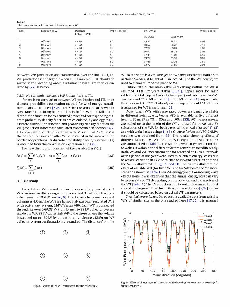
Wake losses: WTs with same rated power are usually availablein different heights, e.g., Vestas V80 is available in five differentheights 60 m, 67 m, 78 m, 80 m and 100 m [32]. WS measurementsare scaled up to the height of the WT and used for power and EYcalculation of the WF, for both cases without wake losses (1)–(3)and with wake losses using (1)–(6). Ct curve for Vestas V80-2.0MWturbines was obtained from [33]. The results showing effects ofdifferent factors, e.g., WF location, WT height and distance on EYare summarised in Table 1. The table shows that EY reduction dueto wakes is variable and different factors contribute to it differently.Both, WS and WD measurement data recorded at 10 min intervalsover a period of one year were used to calculate energy losses dueto wakes. Variation in EY due to change in wind direction enteringthe WF is illustrated in Figs. 9 and 10. The figures illustrate theeffect of variable WD (for fixed WS and for ‘offshore’ and ‘onshore’scenarios shown in Table 1) on WF energy yield. Considering wakeeffects alone it was observed that the annual energy loss can varybetween 2% and 7% depending on the location and parameters ofthe WF (Table 1). The EY reduction due to wakes is variable hence itshould not be generalised for all WFs as it was done in [2,34], rather
Win
d F
arm
pow
er
outp
ut (M
W)
0 50 1007
8
9
10
11
12
13
14
150 200
Wind direction (degrees)
250 300 350 400
Case1
Case2
Case3
Case4
Fig. 9. Effect of changing wind direction while keeping WS constant at 10 m/s (off-shore scenarios).
76 M. Ali et al. / Electric Power System
0 100 200 300 40010
11
12
13
14
15
16
Wind direction (degrees)
Win
d fa
rm p
ow
er
ou
tpu
t (M
W)
Case6
Case5
Case8
Case7
Fig. 10. Effect of changing wind direction while keeping WS constant at 10 m/s(
tcalba7ttt1ara
idlpWfbtt
tc
negligible impact on the annual energy production. As expected
onshore scenarios).
hat the studied WF does not have an offshore transformer. WF isonnected to shore through AC XLPE cable. Power loss calculationsre performed using power flow but with different cable types andengths for each WF collector system. The WF is connected to a slackus such that the voltage at Point of Common Coupling (PCC) islways set to 1 p.u. Cables of cross-sectional area 25 mm2, 50 mm2,0 mm2, 95 mm2 and 120 mm2 [36] within the WF and 150 mm2 forhe main cable connecting WF to the network were used. “Turbineransformers are assumed to have 0.22% resistance and 6% reac-ance at 100 MVA base while grid transformer is assumed to have.5% resistance and 15% reactance at 100 MVA base. No-load lossesre taken to be 0.11% of the capacity of the transformer [37]. As theating of the wind turbines is 2.0 MW, turbine transformers ratedt 2.2 MVA are used. The rating of grid transformer is 25 MVA.”
For energy yield evaluation, only cables with sufficient MVA rat-ng to carry the power that is to be transferred were chosen. A fixedistance of 8 km was used between the WF and the shore. Energy
oss for any collector system varied between 1.40% and 2.08% for thearameters mentioned in the case study (without no-load losses ofT and grid transformers). If however, no-load losses for all trans-
ormers were included then collector network energy losses variedetween 2.16% and 2.84%. Losses with Central configuration collec-or system were the highest while with the Single-sided ring werehe lowest compared to other configurations.
To test the impact of cables sizes and impact of change in dis-ance between WF and shore on losses, the length of the cableonnecting WF with the shore was varied between 8 km and 20 km
0 2 4 6 8 10 12 14 16 180
0.2
0.4
0.6
0.8
1
1.2
1.4
Power Generated (MW)
Po
we
r L
oss (
MW
)
(a)25mm2(inside)120mm2, 20km
50mm2(inside)120mm2, 12km
70mm2(inside)120mm2, 16km
95mm2(inside)120mm2, 20km
120mm2(inside) 150mm2, 8km
(b
Fig. 11. Active power losses for different cable types and distances to
s Research 89 (2012) 70– 79
(in all configurations). Fig. 11 shows that as WF real power gen-eration increased the amount of losses also increased (at unitypower factor). The effect of variation in power losses due to cableparameters, distance and the type of WF collector system are alsoobservable in the figure. It was noticed that for Radial, Star and Cen-tral configuration power losses were very similar for similar typesof cables and lengths used whereas for Single-sided ring configura-tion these losses were slightly different, smaller for some cases.Maximum losses resulted, as expected, when cables of smallestcross-sectional area were used and vice versa. The range of lossescan be used as an indicator of EY sensitivity to collector systemconfiguration and cabling parameters as shown in Fig. 11.
Wind resource availability: Table 2 shows wind resource avail-ability per WT within the studied WF for one year. For 81% of theyear wind potential is sufficient to generate power, i.e. WS withinthe WT operating range. However, due to location of WTs insidethe WF and corresponding wake effects this value is different foreach WT. WTs under wake receive reduced WS (less than 4 m/s insome cases) and hence potential power production for those WTsis lower. It should be also taken into account that wind resourcecan vary by about 10% annually [38]. Table 2 shows that increase ofwind resource by 10% leads to 83% of wind becoming usable for pro-duction of electricity compared to 81% at reference wind resource.This is because increase in WS would place some WTs into operat-ing range while others out of their operating range. From Table 2, itwas observed that wake losses reduce slightly (by 0.7%) from 6.67%to 5.97% when wind resource increased from 0% (reference) to 10%which implies lower WSs causes more wake losses than higher WS.(Note: Increase in wind resource was simulated by increasing eachWS measurement (reference value) by 10% while using the samewind direction associated with it). Overall EY increased by about13.15% due to 10% rise in wind resource (considering wake withmaximum electrical losses).
Wind farm component availability: To evaluate the impact ofcomponent availability in this case study, the availability of onecomponent was set to its typical value (see above) while keepingavailability of other components equal to 100%. It is assumed forthis test that there is no correlation between component availabil-ity and wind power production. Annual energy production is thencalculated for each of the four collector system designs and per-centage of energy loss due to component unavailability calculatedrelatively to “all available” case. The results show that WT trans-former availability (99.998%) and inter-array cable availability have
availability of the WTs (95%) and availability of the main cable(99.8%) has the highest impact, see Table 3. While WT availabil-ity has the same effect on energy losses for all 4 collector system
0 2 4 6 8 10 12 14 16 180
0.2
0.4
0.6
0.8
1
1.2
1.4
Power Generated (MW)
Pow
er
Loss (
MW
)
)25mm2(inside), 25mm2,20km
50mm2(inside), 50mm2,12km
70mm2(inside), 70mm2,16km
95mm2(inside), 95mm2,20km
120mm2(inside),120mm2,8km
shore from the WF for (a) Radial, (b) Single-sided ring system.
M. Ali et al. / Electric Power Systems Research 89 (2012) 70– 79 77
Table 2Wind resource availability on site and for each WT during one year.
5% the amount of energy curtailment rose by 4.41%. The curtailmentincreased by 6.46% in case of 10% rise in wind resource.
Fig. 12. WF Production Probability Distribution Function (WDF) 1 − FX(x), actualTransmission Probability Distribution Function (TDF) 1 − FY(y), New TransmissionProbability Distribution Functions (NTDF) 1 − FZ(z) and Transmission Limit (TL) ofthe case study line.
10% increase 80% 81% 83% 82%
onfigurations, main cable unavailability causes the least energyosses in Single-sided configuration.
The impact of the correlation between wind power productionnd component availability (all components with assumed typ-cal availabilities) on the annual energy losses relatively to “allvailable” case is illustrated in Table 4. Much higher losses due toomponent unavailability are expected if component availability isositively correlated with wind energy production.
Wind energy curtailments: It is assumed that there are other gen-rators situated in the same area as the WF and that the availableransmission capacity from the area is limited to 70 MW. Powerransmission from the WF through the transmission corridor mayot be possible at all times. Wind energy curtailment during theeriods of transmission congestion is considered as an alternativeo transmission line reinforcement. The method for estimation ofind energy curtailment presented in Section 2.5 is applied in this
ase study. When correlation between WP production and TLL is then Section 2.5.1 (27) is used as illustrated in Fig. 7 to deter-ine curtailed energy. Similarly for correlation of −1, curtailment
osses are calculated as described in Section 2.5.1. When there is noorrelation between WP production and TLL then method definedn Section 2.5.2 is used and results are shown in Fig. 12. The fig-re illustrates results of the discrete probabilistic estimation. AsZ(z) = P(Z ≤ z), the value 1 − FZ(C), in Fig. 12 corresponds to therobability that the transmission limit C is exceeded. The shadedrea in Fig. 12 under 1 − FZ(C ≤ z < ∞) is equal to wind energy thatould be curtailed. Availability of WTs is considered between 95%
nd 100% [26]. More possible correlation scenarios are depicted inable 5. Fig. 13 shows effects of these different correlation com-inations on EY from the WF considering 95% WT availability forifferent collector systems. Both wake effects and electrical lossesre included in the results. The influence of latter is very small andherefore hardly visible in the figure. For scenario when WS is theighest, TLL is lowest and WTs are fully available, delivered energy
s very high as shown in Fig. 13 (third combination of correlation
oefficient from Table 5). The range of EY depends on wake effect,
F component availability, curtailment losses and electrical lossesn each cabling structure. For any electrical collector system, whenorrelations between WS, WT availability and TLL were 1 (WS is
able 3mpact of WF component availability on annual energy losses.
Radial Star Central Single-sided
pwt = 95%3.26% 3.26% 3.26% 3.26%
pm = 99.8%0.39% 0.26% 0.65% 0.17%
able 4mpact of correlation between component availability and wind power productionn annual energy losses.
Corr. between comp.availability and WPproduction
Radial Star Central Single-sided
Max wind/Minavailability
12.52% 12.01% 13.04% 11.85%
No correlation 3.66% 3.50% 3.89% 3.41%
80% 83% 80% 79% 83%
high and TLL is highest, WTs are fully available) maximum curtail-ment was required. This amounted to 14.04% (at reference windresource) at 100% WT availability. Conversely, no curtailment wasneeded when correlation between WS and TLL was −1. The amountof curtailment depends on the combination of correlation coeffi-cient which varies with WF location, site measurements and TLLprofile. Increase in wind resource implies rise in power generationhence increase in EY. Since capacity of the line is fixed this yieldsmore energy curtailments. It was observed that for fixed WT avail-ability in Radial collector system when wind resource increased by
0 2 4 6 8 104.4
4.6
4.8
5
5.2
5.4
5.6
5.8x 10
4
No. of combination of Correlation Coefficient
En
erg
y Y
ield
(M
Wh
)
Radial
Star
Central
single-
sided ring
Fig. 13. Effect of WF cabling configuration and correlation coefficient combinationson EY for one year.
78 M. Ali et al. / Electric Power Systems Research 89 (2012) 70– 79
Table 5Combinations for correlation between WS and TLL as well as between WS and WT availability.
Scenario Corr. (WSand TLL)
Corr. (WS and WTavailability)
Scenario Corr. (WSand TLL)
Corr. (WS and WTavailability)
1 1 −1 6 −1 02 1 1 7 0 −1
4
mtsmcattbodswEr1nfhrfacocprocta
A
LA�cvDfF
h�uvxarpˇ
3 −1 1
4 −1 −1
5 1 0
. Conclusion
This paper presented a comprehensive methodology for assess-ent of WF energy losses. A new method to calculate losses due
o reliability of WF components was presented for four collectorystems. Also, a technique to determine amount of energy curtail-ents considering all internal WF losses was given. Correlation
ombinations covering all extreme scenarios were computed tossess the impact of WP production, TLL and WT availability onhe amount of curtailments. In the case studied, energy losses dueo wake varied between 2% and 7%, electrical losses inside the WFetween 2.16% and 2.84%. Losses due to unavailability of WT andther components within the WF were between 0% and 13.05%uring a year depending on component availability, WF collectorystem configuration and correlation between WT availability andind power production. Impact of variation in wind resource on
Y, losses and curtailments were also analysed by increasing windesource by 5% and 10%. A 10% increase in wind resource led to3.15% rise in EY (including losses, WT availability 100%, excludingetwork constraints). Losses due to wind energy curtailments were
ound to be between 0% and 14.04% (at reference wind resource),owever, energy curtailments rose by further 6.46% when windesource increased by 10%. The highest curtailment losses occurredor correlation coefficient equal to 1 between WP, TLL and WTvailability, whereas lowest wind energy curtailment occurred fororrelation coefficient of −1 between WP production and TLL. Basedn sensitivity analysis, it can be concluded that EY should not beomputed as a single value but rather as a range. Methodologiesresented can help WF developers to make more reliable decisionsegarding collector system design, cross-section of cables, heightf WTs, location of the WF and connection with the grid. It can alsoontribute to assess more accurately the option of wind energy cur-ailment against the option of transmission line reinforcement inreas with transmission corridor congestion.
ppendix A.
ist of symbols area of the wind turbine rotor
air densityp power coefficient
wind speed rotor diameter in meters
Y(y) wind farm discrete probability density functionY(y) wind farm production discrete probability distribution
functionY(y) frequency of yy discrete step for FY(y)
incoming wind speed1 wind speed behind one turbine at a distance0 distance
axial induction factorw radius of downstream wake at distance x0s partially shaded
weighting factor
8 0 19 0 0
h upwind turbinej turbine under wakevps,Th partial shadowing of turbines due to turbine hr0 radius of a turbineCt thrust coefficientc wake decay constantI currentR resistancem number of strings/clusters/rowsPstring
losselectrical losses in a string
Pcable to shoreloss
electrical losses in cable to shorePtotal
losstotal electrical losses in a collector system
Ptotal starloss
electrical losses in a star� failure intensity (failures/h)r repair time (h/failure)p availability of each wind farm componentq unavailability of each wind farm componentl length of the cablepc availability of the cableqc unavailability of the cablepwt availability of a wind turbinepmc availability of the main cable of the turbineptr availability of wind turbine transformerp′
wt overall availability of a wind turbineq′
wt overall unavailability of a wind turbinecs component statusesNcs number of component statusesCi status of a cableTi status of a wind turbineKr number of wind turbines in a rowpcs probability of certain combination of component statusesprow(k) probability that in one row k turbines are availableK number of wind turbinesk number of wind turbines available in a rowSWT eq equivalent power curve of a wind turbine�t discretisation stepTc number of hours with transmission congestion�t time stepX amount of power transmitted through bottleneck before
wind power installation in MWY wind power production in MWZ transmission after wind power is installedN number of wind speed measurementsT time periodfX(x) discrete probability density function of power transmis-
sion before wind power is installedFX(x) discrete probability distribution function of power trans-
mission before wind power is installedfZ(z) discrete probability density function of transmission with
wind power installedFZ(z) discrete probability distribution function of transmission
with wind power installed
pWF(k) availability density of star configured wind farmLav range of losses due to unavailability of wind farm compo-
nents
System
Llkp
R
[
[
[
[[
[
[
[
[
[
[
[
[[
[
[
[
[
[
[
[
[
[
[
[
[neering 22 (2002) 23–27.
M. Ali et al. / Electric Power
curtail curtailment lossesc number of components in a rown number of available wind turbines in a wind farmm availability of the main cable to shore
eferences
[1] J.K. Kaldellis, The wind potential impact on the maximum wind energy penetra-tion in autonomous electrical grids, Renewable Energy 33 (2008) 1665–1677.
[2] S.A. Papathanassioua, N.G. Boulaxis, Power limitations and energy yield evalu-ation for wind farms operating in island systems, Renewable Energy 31 (2006)457–479.
[3] A. Albers, G. Gerdes, Wind farm performance verification, in: DEWI MagazineNo. 14, 1999, pp. 24–38.
[4] I. Katic, J. Højstrup, N.O. Jensen, A simple model for cluster efficiency, in: Pro-ceedings of the Eur. Wind Energy Conf. (EWEC), 1986.
[5] K. Rudion, Aggregated modelling of wind farms, Ph.D. dissertation, Otto-von-Guericke-Universitat Magdeburg, Magdeburg, Germany, 2008.
[6] A. Lebioda, K. Rudion, A. Orths, Z. Styczynski, Investigation of disposable reservepower in a large-scale wind farm, in: Proceedings of the IEEE Power Tech, 2005.
[7] M. Ali, J. Matevosyan, J.V. Milanovic, L. Söder, Effect of wake consideration onestimated cost of wind energy curtailments, in: Proceedings of the 8th Int.Workshop on Large Scale Integration of Wind Power and on Transm. Netw. forOffshore Wind Farms, 2009.
[8] R.J. Barthelmie, S.T. Frandsen, M.N. Nielsen, S.C. Pryor, P.E. Rethore, H.E.Jørgensen, Modelling and measurements of power losses and turbulence inten-sity in wind turbine wakes at Middelgrunden offshore wind farm, Wind Energy10 (2007) 517–528.
[9] R.J. Barthelmie, O. Rathmann, S.T. Frandsen, K. Hansen, E. Politis, J.Prospathopoulos, K. Rados, D. Cabezón, W. Schlez, J. Phillips, A. Neubert, J.G.Schepers, S.P. van der Pijl, Modelling and measurements of wakes in large windfarms, Journal of Physics: Conference Series 75 (2007).
10] M. Méchali, R. Barthelmie, S. Frandsen, L. Jensen, P.-E. Réthoré, Wake effectsat Horns Rev and their influence on energy production, in: Proceedings of theEuropean Wind Energy Conference and Exhibition, 2006.
11] Danish Wind Industry Association, Roughness Classes and Roughness LengthTable, 2003 <http://www.talentfactory.dk/en/stat/unitsw.htm> (accessed02.08.09).
12] WAsP – The Wind Atlas Analysis and Application Program, Wake EffectModel, 2007 <http://www.wasp.dk/Products/WAsP/WakeEffectModel.html>(accessed 03.08.09).
13] T. Burton, Wind Energy Handbook, John Wiley & Sons, Ltd., Chichester, 2001.14] G. Mosetti, C. Poloni, B. Diviacco, Optimization of wind turbine positioning in
large wind farms by means of a genetic algorithm, Journal of Wind Engineeringand Industrial Aerodynamics 51 (1994) 105–116.
15] S. Frandsen, M.L. Thogersen, Integrated fatigue loading for wind turbines in
wind farms by combining ambient turbulence and wakes, Wind Engineering23 (1999) 327–339.
16] P. Frohboese, C. Schmuck, Thrust coefficients used for estimation of wake effectsfor fatigue load calculation, in: Proceedings of the European Wind Energy Con-ference, 2010.
18] G.W. Ault, G. Quinonez-Varela, O. Anaya-Lara, J.R. McDonald, Electrical collectorsystem options for large offshore wind farms, IET Renewable Power Generation1 (2007) 107–114.
19] J. Ribrant, L.M. Bertling, Survey of failures in wind power systems with focuson Swedish wind power plants during 1997–2005, IEEE Transactions on EnergyConversion 22 (2007) 167–173.
20] I.-S. Ilie, G. Chicco, Protections impact on the availability of a wind power plantoperating in real conditions, in: Proceedings of the IEEE Power Tech, 2009.
21] A.U.E. Spahic, V. Buchert, J. Hanson, I. Jeromin, G. Balzer, Reliability model oflarge offshore wind farms, in: Proceedings of the IEEE Power Tech, 2009.
22] P.J. Cameron, Combinatorics: Topics, Techniques, Algorithms (1994) 40–44.23] C. Shuyong, D. Huizhu, B. Xaiomin, Z. Xiaoxin, Evaluation of grid connected
wind power plants, in: Proceedings of the Int. Conf. on Power Syst. Technol.(PowerCon), 1998, pp. 1208–1212.
24] G. Chicco, P. Di Leo, I.-S. Ilie, F. Spertino, Operational characteristics of a 27-MWwind farm from experimental data, in: Proceedings of the 14th IEEE Mediter-ranean Electrotech. Conf. (Melecon), 2008, pp. 520–526.
25] K.F. Utsurogi, P. Giorisetto, Development of a new procedure for reliability mod-elling of wind turbine generators, IEEE Transaction on Power Apparatus andSystems PAS-102 (1983) 134–143.
26] Elforsk, Operation follow up of wind turbines, wind statistics, 2003<www.elforsk.se/varme/varm-vind.html> (accessed 12.10.09) (in Swedish).
27] T. Ackermann, Wind Power in Power Systems, John Wiley & Sons, Ltd., Chich-ester, 2005.
28] J. Matevosyan, Wind power integration in power systems with transmissionbottlenecks, Ph.D. dissertation, School of Elect. Eng., Royal Institute of Tech.,Stockholm, Sweden, 2006.
29] E. Centeno Lopez, T. Ackermann, Grid Issues of Electricity Production based onRenewable Energy Sources in Spain, Portugal, Germany and United Kingdom,Statens Offentliga Utredningar, Stockholm, 2008.
30] P. Gardner, L.M. Craig, G.J. Smith, Electrical systems for offshore wind farms, in:Proceedings of the 20th British Wind Energy Assoc. (BWEA) Conf., 1998.
31] E. Spahic, A. Underbrink, V. Buchert, J. Hanson, I. Jeromin, G. Balzer, Reliabilitymodel of large offshore wind farms, in: Proceedings of the IEEE Power Tech,2009.
32] Vestas Wind Systems A/S, V80-2.0MW Brochure, 2009 <http://www.vestas.com/en/wind-power-solutions/wind-turbines/2.0-mw.aspx> (accessed20.08.09).
33] L.E. Jensen, C. Morch, P.B. Sorensen, Wake measurements from the Horns Revwind farm, in: Proceedings of the European Wind Energy Conference (EWEC),2004.
34] J.R. Mclean, Equivalent Wind Power Curves, Garrad Hassan and Partners Ltd.,Tradewind Report – WP2.6, 2008.
35] T. Ackermann, Transmission systems for offshore wind farms, IEEE Power Engi-
36] ABB, XLPE Cable Systems – User’s Guide, 2006 (accessed 14.06.09).37] L.W. Pierce, Transformer design and application considerations for nonsinu-
soidal load currents, IEEE Transactions on Industry Applications 32 (1996).38] A. Albers, Wind index 1998, in: DEWI Magazine No. 14, 1999, pp. 36–38.