24
Probabilistic Link Properties Octav Chipara

Probabilistic Link Properties
Octav Chipara
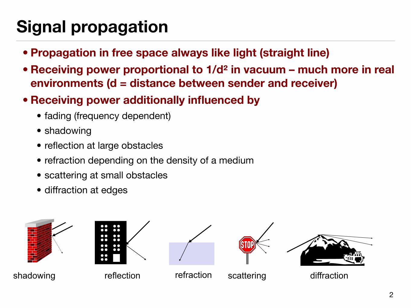
Signal propagation• Propagation in free space always like light (straight line)• Receiving power proportional to 1/d² in vacuum – much more in real environments (d = distance between sender and receiver)
• Receiving power additionally influenced by• fading (frequency dependent)• shadowing• reflection at large obstacles• refraction depending on the density of a medium• scattering at small obstacles• diffraction at edges
reflection scattering diffractionshadowing refraction
2

Physical impairments: Fading (1)
short term fading
long termfading
t
power
3
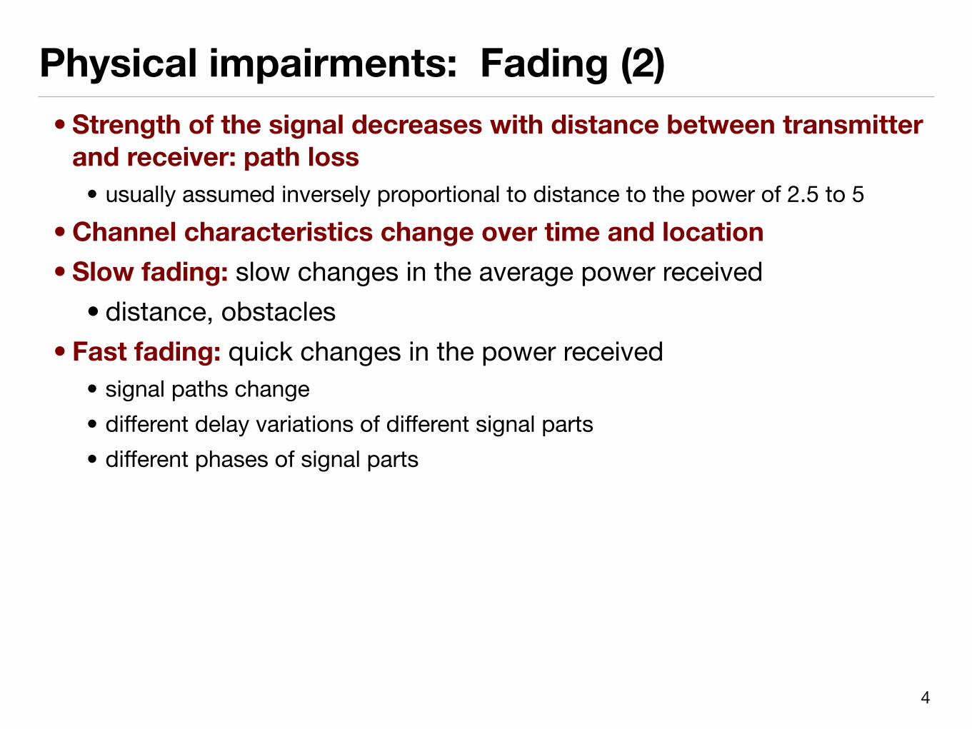
Physical impairments: Fading (2)• Strength of the signal decreases with distance between transmitter and receiver: path loss
• usually assumed inversely proportional to distance to the power of 2.5 to 5• Channel characteristics change over time and location• Slow fading: slow changes in the average power received
• distance, obstacles• Fast fading: quick changes in the power received
• signal paths change• different delay variations of different signal parts• different phases of signal parts
4
Physical Impairments: Noise• Unwanted signals added to the message signal• Many potential sources of noise
• natural phenomena such as lightning • radio equipment, spark plugs in passing cars, wiring in thermostats, etc.
• Modeled in the aggregate as a random signal in which power is distributed uniformly across all frequencies (white noise)
• Signal-to-noise ratio (SNR) often used as a metric in the assessment of channel quality
5

Physical Impairments: Interference• Signals at roughly the same frequencies may interfere with one another• Example: IEEE 802.11b and Bluetooth devices, microwave ovens, some
cordless phones• CDMA systems (many of today’s mobile wireless systems) are typically
interference-constrained• Signal to interference and noise ratio (SINR) is metric used in assessment of channel quality
6
SNIRs,r =RSSs,r
Noise+ Interference

• Signal can take many different paths between sender and receiver due to reflection, scattering, diffraction
• Time dispersion: signal is dispersed over time• interference with “neighbor” symbols, Inter Symbol Interf. (ISI)
• The signal reaches a receiver directly and phase shifted• distorted signal depending on the phases of the different parts
Multipath propagation
signal at sendersignal at receiver
LOS pulsesmultipath
pulses
7

Signal propagation: Real world example
distance
sender
transmission
detection
8

Parametric propagation models• Free space propagation model
• when not in free-space, the path loss exponent (2) is higher
• Log-normal propagation model
• - Gaussian RV with mean zero, it accounts for shadowing• n - path loss exponent, depends on environment (e.g., 3--6 indoors)• d0 - reference distance in far field • PL - path loss
9
PL(d) = PL(do
) ⇤✓d0d
◆2
PL(d) = PL(do
) + 10nlog10
✓d0
d
◆+X
�
X�
Radio signal propagation•Model signal strength (and its variation) at a distance
• useful for localization applications, coverage, etc• networks with mobile users
• Model signal strength (and its variations) at a fixed distance• useful for networking protocols (routing, ARQ, etc)• fixed networks
10

Log-normal path model
11
PL(d) = PL(do
) + 10nlog10
✓d0
d
◆+X
�

12*Zhou et. al. 04
Non-isotropic connectivity

13
Non-isotropic connectivity (2)

14*Cerpa et. al. 03
Attenuation over distance

15
Impact of antenna height

Transitional region (aka grey region)
16
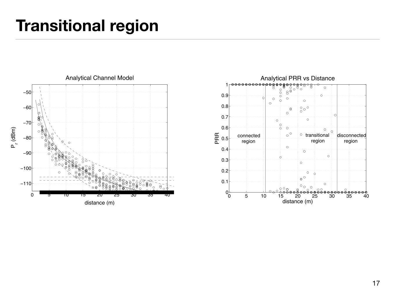
Transitional region
17
0 5 10 15 20 25 30 35 40
−110
−100
−90
−80
−70
−60
−50
distance (m)
Pr (
dBm
)
Analytical Channel Model
Fig. 1. Channel Model, q = 4, � = 4, Sw = 0 gEp
different radios and environments. The model presented inthis work does not consider interference, which is part of ourfuture work. Nevertheless, in scenarios where the traffic andcontention are relatively light; a very reasonable assumptionfor many classes of data-centric sensor networks, our modelprovides an accurate estimate of the links’ quality.
III. DELIMITING RESPONSIBILITIES: THE CHANNEL ANDTHE RADIO
The transitional region is the result of placing specific de-vices, for example MICA2 motes, in an specific environment,like the aisle of a building. With the intend of analyzing howthe channel and the radio determine the transitional region;first, we define models for both elements, to subsequentlystudy their interaction.
A. The Wireless ChannelWhen an electromagnetic signal propagates, it may be
diffracted, reflected and scattered. These effects have twoimportant consequences on the signal strength. First, thesignal strength decays exponentially with respect to distance.And second, for a given distance g, the signal strength israndom and log-normally distributed about the mean distance-dependent value.Due to the unique characteristics of each environment, most
radio propagation models use a combination of analyticaland empirical methods. One of the most common radiopropagation models is the log-normal shadowing path lossmodel [13]2. This model can be used for large and small[11] coverage systems; furthermore, empirical studies [12]have shown the the log-normal shadowing model providesmore accurate multi-path channel models than Nakagami andRayleigh for indoor environments. The model is given by:
SO(g) = SO(g0) + 10qorj10(g
g0) +[� (1)
2The model is valid only for the transmission frequency and environmentwhere the data was gathered.
0 5 10 15 200
0.1
0.2
0.3
0.4
0.5
0.6
0.7
0.8
0.9
1
SNR (dB)P
RR
Analytical Radio Model
Zero Packet Reception
Perfect Packet Reception
Fig. 2. Radio Model: Non-Coherent FSK, NRZ radio, i = 50 e|whv
Where g is the transmitter-receiver distance, g0 a referencedistance, q the path loss exponent (rate at which signaldecays), and [� a zero-mean Gaussian RV (in dB) withstandard deviation � (shadowing effects)3. In the most generalcase, [� is a random process that is a function of time, but,since we are not assuming dynamic environments, we modelit as a constant random variable over time for a particular link.The received signal strength (Su) at a distance g is the
output power of the transmitter minus SO(g). Figure 1 showsan analytical propagation model for q = 4, � = 4, SO(g0) =55 dB and an output power of 0 dBm.
B. The RadioTo facilitate the explanation of the radio model, this sub-
section assumes NRZ encoding. Section IV provides modelsfor other encoding schemes.The steps followed to derive the radio model are similar
to the ones in [9]. Let Sl be a Bernoulli random variable,where Sl is 1 if the packet is received and 0 otherwise. Then,for u transmissions, the packet reception rate is defined by1u
Pul=1 Sl. Since Sls are i.i.d. random variables, by the weak
law of large numbers PRR can be approximated by H[Sl],where H[Sl] is the probability of successfully receiving apacket.If NRZ is used and 1 Baud = 1 bit, the probability s of
successfully receiving a packet is:
s = (1� Sh)8c(1� Sh)
8(i�c)
= (1� Sh)8i (2)
Where i is the frame size4, c is the preamble (both inbytes), and Sh is the probability of bit error. Sh depends on themodulation scheme, for non-coherent FSK (modulation usedin MICA2 motes), Sh is given by:
Sh =1
2exp�
�2 (3)
3q and � are obtained through curve fitting of empirical data; SO(g0) canbe obtained empirically or analytically.4A frame consists of: preamble, network payload (packet) and CRC
519519
0 5 10 15 20 25 30 35 40
−110
−100
−90
−80
−70
−60
−50
distance (m)
Pr (
dBm
)
Analytical Method to Determine Regions in Wireless Links
µ µ+2σ µ−2σ
noise floor (Pn)
Pn + γ
U
Pn + γ
L
Beginning of Transitional Region
End of Transitional Region
Fig. 3. Analytical Observation of the Transitional Region
Where � is the HeQ0ratio. Hence, the PRR s is defined as:
s = (1�1
2exp�
�2 )8i (4)
Nevertheless, most commercial radios do not provide theHeQ0metric, but the RSSI (Received Signal Strength Indicator)
of the received signal. The RSSI measurements can be usedto determine the SNR (Signal-to-Noise ratio); henceforth, inthis work, the expression based on He
Q0are converted to SNR.
The relation between SNR and HeQ0is given by:
VQU =He
Q0
U
EQ(5)
Where U is the data rate in bits, and EQ is the noisebandwidth. For MICA2 motes, U = 19.2 kbps and EQ = 30kHz. Finally, the PRR s in terms of the SNR (�) is given by:
s = (1�1
2exp�
�2
10=64 )8i (6)
The curve in figure 2 shows equation 6 (receiver response)for a frame size of 50 bytes. As we shall see later, this curveplays an important role in determining the different regions.
C. The Noise FloorAnother important element that determines the transitional
region is the noise floor, which depends on both, the radioand the environment. The temperature of the environment in-fluences the thermal noise generated by the radio components(noise figure), the environment can further influence the noisefloor due to interfering signals. When the receiver and theantenna have the same ambient temperature the noise floor isgiven by [13]:
Sq = (I + 1)nW0E (7)
Where I is the noise figure, n the Boltzmann’s constant,W0 the ambient temperature and E the equivalent bandwidth.MICA2s use the Chipcon CC1000 radio [14], which has anoise figure of 13 dB and a system noise bandwidth of 30
0 5 10 15 20 25 30 35 400
0.1
0.2
0.3
0.4
0.5
0.6
0.7
0.8
0.9
1
distance (m)
PR
R
Analytical PRR vs Distance
connected region
transitional region
disconnected region
Fig. 4. Analytical PRR vs Distance, obtained through equation 9
kHz. Considering an ambient temperature of 300 �K (27 �C,75 �F) and no interference signals, the noise floor is -115 dBm.The noise figure provided in [14] is only for the chip,
and does not include losses due to board implementations.Hence, the noise figure of the final hardware will be higher.In section V, the noise floor is redefined based on empiricalmeasurements.
D. Putting all TogetherGiven a transmitting power Sw, the SNR � at a distance g
is:
�(g)gE = Sw gE � SO(g)gE � Sq gE (8)
Henceforth, the PRR at a distance g for the encoding andmodulation assumed in this section is:
s(g) = (1�1
2exp�
�(g)2
10=64 )8i (9)
With the aim of obtaining the radius of the different regions,let us bound the connected region to PRRs greater than 0.9,and the transitional region to values between 0.9 and 0.1. Ifwe let �X gE and �O gE be the SNR values for PRRs of 0.9and 0.1 respectively, then from equation 9 we obtain:
�X gE = 10orj10(�1=28 oq(2(1� 0=918i )))
�O gE = 10orj10(�1=28 oq(2(1� 0=118i )))
(10)
The previous equations determine the bounds of the regionsin the radio model. Now, let us analyze how these boundsinteract with the channel model to define the radius of thedifferent regions at the link layer.Due to the gaussian characteristic of log-normal shadowing
in the path loss model, the received signal strength Su can bebounded within ±2�, i.e. S (�� 2� ? Su ? �+ 2�) = =955.If we let SO(g) = SO(g0) + 10qorj10(
gg0), then, for a given
output power Sw, the received power Su at a distance g isbounded by:
520520

Transitional region
18
0 5 10 15 20 25 30 35 40
−110
−100
−90
−80
−70
−60
−50
distance (m)
Pr (
dBm
)
Analytical Method to Determine Regions in Wireless Links
µ µ+2σ µ−2σ
noise floor (Pn)
Pn + γ
U
Pn + γ
L
Beginning of Transitional Region
End of Transitional Region
Fig. 3. Analytical Observation of the Transitional Region
Where � is the HeQ0ratio. Hence, the PRR s is defined as:
s = (1�1
2exp�
�2 )8i (4)
Nevertheless, most commercial radios do not provide theHeQ0metric, but the RSSI (Received Signal Strength Indicator)
of the received signal. The RSSI measurements can be usedto determine the SNR (Signal-to-Noise ratio); henceforth, inthis work, the expression based on He
Q0are converted to SNR.
The relation between SNR and HeQ0is given by:
VQU =He
Q0
U
EQ(5)
Where U is the data rate in bits, and EQ is the noisebandwidth. For MICA2 motes, U = 19.2 kbps and EQ = 30kHz. Finally, the PRR s in terms of the SNR (�) is given by:
s = (1�1
2exp�
�2
10=64 )8i (6)
The curve in figure 2 shows equation 6 (receiver response)for a frame size of 50 bytes. As we shall see later, this curveplays an important role in determining the different regions.
C. The Noise FloorAnother important element that determines the transitional
region is the noise floor, which depends on both, the radioand the environment. The temperature of the environment in-fluences the thermal noise generated by the radio components(noise figure), the environment can further influence the noisefloor due to interfering signals. When the receiver and theantenna have the same ambient temperature the noise floor isgiven by [13]:
Sq = (I + 1)nW0E (7)
Where I is the noise figure, n the Boltzmann’s constant,W0 the ambient temperature and E the equivalent bandwidth.MICA2s use the Chipcon CC1000 radio [14], which has anoise figure of 13 dB and a system noise bandwidth of 30
0 5 10 15 20 25 30 35 400
0.1
0.2
0.3
0.4
0.5
0.6
0.7
0.8
0.9
1
distance (m)
PR
R
Analytical PRR vs Distance
connected region
transitional region
disconnected region
Fig. 4. Analytical PRR vs Distance, obtained through equation 9
kHz. Considering an ambient temperature of 300 �K (27 �C,75 �F) and no interference signals, the noise floor is -115 dBm.The noise figure provided in [14] is only for the chip,
and does not include losses due to board implementations.Hence, the noise figure of the final hardware will be higher.In section V, the noise floor is redefined based on empiricalmeasurements.
D. Putting all TogetherGiven a transmitting power Sw, the SNR � at a distance g
is:
�(g)gE = Sw gE � SO(g)gE � Sq gE (8)
Henceforth, the PRR at a distance g for the encoding andmodulation assumed in this section is:
s(g) = (1�1
2exp�
�(g)2
10=64 )8i (9)
With the aim of obtaining the radius of the different regions,let us bound the connected region to PRRs greater than 0.9,and the transitional region to values between 0.9 and 0.1. Ifwe let �X gE and �O gE be the SNR values for PRRs of 0.9and 0.1 respectively, then from equation 9 we obtain:
�X gE = 10orj10(�1=28 oq(2(1� 0=918i )))
�O gE = 10orj10(�1=28 oq(2(1� 0=118i )))
(10)
The previous equations determine the bounds of the regionsin the radio model. Now, let us analyze how these boundsinteract with the channel model to define the radius of thedifferent regions at the link layer.Due to the gaussian characteristic of log-normal shadowing
in the path loss model, the received signal strength Su can bebounded within ±2�, i.e. S (�� 2� ? Su ? �+ 2�) = =955.If we let SO(g) = SO(g0) + 10qorj10(
gg0), then, for a given
output power Sw, the received power Su at a distance g isbounded by:
520520
• Length of the transitional region increases with• increases in shadowing => impact of multi-path• decreases in path loss coefficient

Prevalence of good, bad, and intermediary links
19
0.0 0.2 0.4 0.6 0.8 1.0Reception Ratio
0
20
40
60
80
100
% o
f Li
nks
MirageUniversityLake
(a) University and Mirage IPI=10ms,Lake IPI=50ms
0.0 0.2 0.4 0.6 0.8 1.0Reception Ratio
0
20
40
60
80
100
% o
f Li
nks
IPI=10msIPI=1s
(b) University
0.0 0.2 0.4 0.6 0.8 1.0Reception Ratio
0
20
40
60
80
100
% o
f Li
nks
IPI=10msIPI=15s
(c) Mirage
Figure 2. Reception ratio and the CDF of proportion of links in the three testbeds for channel 26. The percent-age of intermediate links is small compared to good and bad links, and it increases as the inter-packet intervalincreases.
0.0 0.2 0.4 0.6 0.8 1.0Reception Ratio
0
20
40
60
80
100
% o
f Li
nks
Channel=16Channel=26
Figure 3. CDFs of link qualities in Mirage on Chan-nels 16 and 26. The proportion of perfect links ismore in channel 26 than in channel 16: 60% in 26and 12% in 16 of all the communicating links.
creasing the IPI from 10ms to 1 second increases thepercentage of intermediate links from 5% to 19% in theuniversity testbed. Mirage increases from 19% to 23%as IPI increases from 10ms to 15 seconds. As the re-ception ratio is calculated over 200 packets, the packetinterval determines the total measurement time: an ex-periment with IPI of 10ms takes 2 seconds while onewith an IPI of 15 seconds takes 50 minutes.
Timing is not the only factor that affects link distribu-tions. Figure 3 shows how channel selection changes thePRR distribution in Mirage. Channel 16 has far fewerperfect links than channel 26: 60% in channel 26 andonly 12% in channel 16. Correspondingly, 35% of thecommunicating channel 16 links are intermediate, com-pared to 17% of channel 26 links.
These results lead to two major observations. First,frequency affects link distributions. While this is notsurprising, learning why is an important step to betterunderstand wireless behavior. We defer this question toSection 5.
Second, the percentage of intermediate links dependson the timescale over which a protocol measures them.Over shorter periods, links have a higher chance of be-ing perfect or non-existent. Over longer periods, thechance of being intermediate increases. In Section 5,we examine this behavior more closely, finding it is dueto links on the edge of reception sensitivity, moving be-tween poor and good states. As the measurement periodincreases, so does the chance of observing a transition.
While this is a simple observation, it has deep implica-tions for wireless protocol design: the data plane mayobserve different link qualities than the control planewhich sends link measurement packets.
3 Measuring BurstinessThis section defines b, a metric to measure links’
bursty behavior. We show how to compute b and ob-serve that many Mirage links on channel 26 have high bvalues.
3.1 Conditional DeliveryFirst, we need a way to concisely describe link be-
havior observed in packet traces. Conditional packet de-livery functions (CPDFs) provide a succinct way to de-scribe the durations of packet delivery correlations [20].The conditional packet delivery function C(n) is theprobability the next packet will succeed given n con-secutive packet successes (for n > 0) or failures (forn < 0). For example, C(5) = 83% means that the proba-bility a packet will arrive after five successful deliveriesis 83%, while C(�7) = 18% means that the probabilityafter seven consecutive losses is 18%.
Figure 4 shows four sample CPDFs. A link with in-dependent losses will have a flat CPDF: the probabilityof reception is independent of any history. In contrast,Figure 4(a) shows the CPDF of the ideal bursty link;successes and failures happen in bursts. There is aninherent timescale assumption in this description: theburst length must be longer than the CPDF x-axis range.Burst lengths that are small enough to occur within theCPDF range make a link look more independent.
We program nodes on the Mirage testbed to broad-cast 100,000 packets with an inter-packet interval of10ms, one node at a time, and use the packet traces tocalculate link CPDFs. We use 100,000 packets to pro-vide reasonable confidence intervals to the CPDF val-ues. In addition, each element in a CPDF has a mini-mum of 100 data points.1 Figures 4(b)-4(d) show the
1100 data points gives a worst case 95% confidence inter-val of [p-0.1,p+0.1], where p is the empirical conditional prob-ability.
0.1 0.2 0.3 0.4 0.5 0.6 0.7 0.8 0.9
1
0 0.1 0.2 0.3 0.4 0.5 0.6 0.7 0.8 0.9 1
Com
plem
enta
ry C
DF
Packet Loss
In DoorOut Door
Habitiat
Figure 4: Packet Loss with 4b6bcoding, high Tx power
0.1 0.2 0.3 0.4 0.5 0.6 0.7 0.8 0.9
1
0 0.1 0.2 0.3 0.4 0.5 0.6 0.7 0.8 0.9 1
Com
plem
enta
ry C
DF
Packet Loss
High Tx Power(0)Medium Tx Power(50)
Low Tx Power(90)
Figure 5: Packet loss v.s. Tx powerin I, 4b6b coding
0.1 0.2 0.3 0.4 0.5 0.6 0.7 0.8 0.9
1
0 0.1 0.2 0.3 0.4 0.5 0.6 0.7 0.8 0.9 1
Com
plem
enta
ry C
DF
Packet Loss
4BSBSECDED
Manchester
Figure 6: Packet loss v.s. codingschemes in I, high Tx Power
packet delivery at the physical layer, we had to disable theTinyOS MAC layer. Because we have a single transmitter,the MAC layer’s carrier-sense and collision avoidance strat-egy is effectively non-operational. However, we had to mod-ify TinyOS’s MAC so that its acknowledgment mechanismcould be optionally disabled.
Using this basic setup, we varied three factors in our ex-periments: the choice of environments, the physical layercoding schemes, and the transmit power settings.
We chose three environments for experimentation:
• I is an office building. The choice of this environmentis motivated by in-building sensing applications [16].In this office building, we placed our setup in a longhallway (2 meter by 40 meter) (Figure 1). This hall-way poses a particularly harsh wireless environment,because of significant likelihood of multi-path reflec-tions from the walls. This particular placement doesnot result in signal attenuation through walls or otherobstacles, but may suffer from interference with otherelectronic devices (this is a somewhat remote possibil-ity; we were operating the radios in the 433MHz band,which is allocated for amateur radio use in the US).
• H is a 150m by 150m segment of a local state park(Figure 2). The choice of this environment is moti-vated by several recent efforts that seek to monitorhabitats [1]. To conduct our experiment, we chosea downhill slope with foliage and rocks. As with I,multi-path due to scattering from foliage and rock wouldcontribute to a fairly harsh wireless communication inthis environment as well.
• Finally, O is a large, spacious parking lot (150m by150m). Compared to the our two environments, it isrelatively benign (no obstacles, and multi-path onlydue to ground reflections). O provides some contextfor interpreting our other environments; it is hard toenvision a sensor net in an open parking lot since therewould be no interesting phenomena to sense.
Many of our experiments were conducted on different days.In conducting our experiments, we tried to keep the envi-ronment’s gross characteristics as consistent as possible (inaddition to making sure we were able to replicate placementexactly, using markers). For example, in I, we kept all thedoors along the hallway closed, and conducted our experi-ments at late night hours, to minimize (but of course, notcompletely eliminate) interference from human activity. Inthis sense, our measurements from I and H report their“quiescent” state.
The second factor we varied in our experiments was thephysical layer coding scheme. The default TinyOS SECDEDcoding encodes each byte into 24 bits. SECDED can detect2 bit errors and correct one bit error. By contrast, the 4-bit/6-bit (or 4b6b) scheme encodes one 8-bit byte into 12bits, with the capability of detecting 1 bit error out of 6bits. The well-known Manchester coding scheme encodeseach byte into 16 bits, with capability of detecting erro-neous bit out of 2 bits. All of these coding schemes areDC-balanced. Of these schemes, 4b6b is the least error tol-erant, followed by Manchester and SECDED. However, it isthe most bandwidth efficient, using the fewest extra encod-ing bits.
Finally, the motes have hardware that allows discrete con-trol of transmit powers. Specifically, the motes have a poten-tiometer that regulates the voltage delivered to the trans-mitter. Rather than explore the entire range of transmitpower settings, we chose three qualitatively different set-tings: high (potentiometer 0), medium (potentiometer 50),and low (potentiometer 90).
Each experiment takes approximately 8 hours, though inthe following sections, the analysis is based on the data in awindow from hour 2 to hour 4. This allowed us to have ananalyzable data set; we also examined other time windowsand found the results to be in qualitative agreement.
4.2 Aggregate Packet Delivery PerformanceOur basic metric for packet delivery performance is packet
loss: the fraction of packets not successfully received (i.e.,passed CRC check) within some time window, where thetime window will be clear from the context.
Sometimes, we measure its complement, the packet recep-tion rate. We measure packet loss by analyzing the sequencenumbers received at each receiver.
We first discuss a very gross measure of overall packetdelivery performance to summarize our findings. For eachexperiment, we plot the distribution of packet loss within atwo hour frame (i.e., 7200 transmitted packets) across allthe receivers. Such a metric can bring out the variability(or conversely the uniformity) of packet loss radially from anode.
Figures 4 through 6 illustrate the aggregate packet deliv-ery performance for different environments, coding schemesand transmission power settings. Several interesting obser-vations emerge from these graphs. These observations pro-vide fodder for a more detailed analysis of packet loss. (Theactual distributions plotted in all of these graphs is likely tobe slightly different than if we had had more sample points
• A significant fraction of links fall within the transitional region• these links are important for protocols but hard to utilize
decreases b – packet events become less correlated asthe interval between the events increases. This suggeststhat looking at the decay of b can show when a link canresume transmissions upon a packet failure.
The path and link cost results come from the traceswith which we calculated b. This raises the questionof whether the same information from b can predict theperformance of a protocol that runs after the networkhas been measured. Changing the pause interval of astandard sensornet collection protocol and running it inreal-time on a testbed decreases the overall network de-livery cost by 15%. This shows that b gives further in-sight into a network’s characteristics and into how pro-tocol designers can tune their protocols according to thenetwork to improve performance.
Exploring the possible causes of burstiness in802.15.4 reveals that it is due to channel variations, inthe form of changes in received signal strength. Aschannel variations are common in wireless networks, bmay be more broadly applicable than just 802.15.4. Ex-amining data from 802.11b studies [7, 23], we find that802.11b in both indoor and outdoor environments ex-hibits burstiness and that b can predict protocol perfor-mance in 802.11b networks.
Measuring burstiness and its effect on network per-formance suggest we need to rethink current approachesto wireless protocol design and analysis: reasoningabout how protocols perform requires an understandingof fine-grained temporal properties.
The rest of this paper is structured as follows. Sec-tion 2 looks at reception ratios of wireless links. ThenSection 3 quantifies link burstiness and introduces b.Section 4 presents a simple algorithm that can benefitfrom a knowledge of b. Section 5 investigates the causesof burstiness and Section 6 shows that this burstiness isrelevant to different link layers. Section 7 further evalu-ates b’s effect on protocols. Finally, Section 8 discussesrelated work and concludes.
2 802.15.4 Packet DeliveryThis section introduces 802.15.4, its packet delivery
behavior, and the testbeds we use. It also defines theterminology to describe links with different receptionsand observes that the timescale of measurements affectstestbed reception results.
2.1 802.15.4 and Testbeds802.15.4 is an IEEE PHY-MAC standard for low
power, low datarate networks. It has a datarate of250kbps and a range of approximately one hundred me-ters. It provides 16 channels, numbered 11-26 in the 2.4GHz band (2405 MHz - 2480 MHz). The channels are5 MHz apart, overlapping with 802.11b and 802.15.1(Bluetooth).
We measured 802.15.4 using three wireless sensornettestbeds. Most experiments use the 100 node Intel Mi-rage testbed [14]. We also present results from a 30 nodeuniversity testbed; the Mirage and university nodes are
10% 90%0% 100%
Intermediate GoodPoor
No Link Perfect
Packet Reception Rate
Figure 1. Terminology used to describe links basedon PRR. Poor links have a PRR < 10%, intermediatelinks are between 10% and 90%, and good links are> 90%. A PRR of 100% is a perfect link. A linkthat receives one or more packets is a communicatinglink.
on the ceiling. Finally, we examine an outdoor 20 nodedry lake testbed in which nodes were arranged in a line,spaced 4 feet apart and all had clear line of sight. Allnodes in these experiments ran TinyOS [13] and usedthe CC2420 802.15.4 chip [6], which provides variabletransmit power control from 0dBm to -20dBm.
2.2 Packet DeliveryPrior studies of wireless networks have observed that
links have a wide range of packet reception ratios (PRR)which can vary significantly over time [2, 4, 23, 21]. Todetermine whether 802.15.4 behaves similarly, we mea-sured reception ratios in the university, Mirage and laketestbeds. In the rest of this paper, we describe links aspoor, intermediate, good, or perfect in terms of PRR, us-ing the definitions shown in Figure 1; we use the termslink quality and packet reception ratio interchangeably.Since prior studies have shown that 802.15.4 links canvary significantly over time [21], we measured receptionratios over different time scales by sending 200 broad-casts with varying inter-packet intervals (IPI, the timebetween packet transmissions). We used inter-packet in-tervals ranging from 10ms up to 15 seconds. All pack-ets used the standard TinyOS CSMA layer and we con-trolled transmission timing so there would be no colli-sions. The lack of a wired backchannel prevented lakenodes from having an IPI below 50ms.
Figure 2(a) shows the reception ratio distribution inthe three testbeds on channel 26 with small inter-packetintervals. About 55% of all node pairs in the Mirageand university testbeds can communicate, while 90% ofthe pairs in the lake testbed can communicate. Of thesecommunicating links, 19% in Mirage, 14% in the lake,and 5% in the University are intermediate. These num-bers are lower than what has been observed in other net-works. Even the 19% in Mirage is much less than the50% reported for earlier sensor platforms and the 58%reported for Roofnet [2]. Compared to these other net-works, 802.15.4 has a much sharper reception distribu-tion. While intermediate links do not dominate the net-work, wireless protocols cannot simply ignore them.
2.3 Time and Frequency EffectsFigures 2(b) and 2(c) show how the time interval be-
tween packets affects the reception ratio distribution. In-
19%14%5%

Link symmetry
20
(a) Wednesday (b) SaturdayFigure 10. PRR Asymmetry for 30 nodes in the Mirage testbedover a 200 packet unicast burst for two different trials. The30 nodes were a subset of the testbed nodes that covered theentire lab area. While they are shown in a circle solely for visu-alization purposes, nodes close to each other on the circle wereclose to each other in the testbed. Nodes having asymmetry areconnected using a colored line, where the red end of the line isthe node that had trouble receiving packets. A larger gradienton the line indicates higher asymmetry. While each trial hada significant number of asymmetric links, there are only two(N14-N26 and N17-N4) present in both.
metrics links occur in both experiments. This suggests that theremay be significant temporal effects in link asymmetry.
To determine the time scale of variations in PRR asymmetry, weexamined the data from the round-robin experiment used in Fig-ure 4 and calculated link asymmetry over four separate one hourperiods. Figure 11 shows the results. It is clear that a few linkssuch as N17!N4 are consistently asymmetric while some such asN18!N10 are not. Furthermore, the number of asymmetric linksis much smaller. These results suggest that there are significant dif-ferences between long-term and short-term link behavior.
Since Section 4 showed that temporal variations in RSSI werethe cause of temporal changes in PRR, it is a reasonable hypothesisthat it is the cause here as well. Figure 4 supports this hypothesis:in the second hour, node 4 is able to receive packets from node 30because the RSSI increased to be mostly -90dBm readings ratherthan -91dBm, as also seen in Figure 11(b).
Table 3. Distribution of estimated noise floor across the motesin the Mirage round robin experiment. Only 26 of the 30 nodesreported noise data.
SSI (dBm) -98 -97 -96 -95 -94 -93 -92# Nodes 5 8 4 3 2 3 1
6.2 Causes of AsymmetryTogether, the RSSI temporal variation results from Section 4 and
the inter-node noise variation results from Section 5 present a pic-ture of what causes asymmetric links and why they might changeover time. Table 3 shows the distribution of noise floors in the Mi-rage round-robin experiment. Just as with the university testbed,there are significant inter-node variations, which would affect SNRand therefore lead to PRR asymmetry. However, in comparison tothe university testbed (Table 1), they have a larger range and arealso several dBm higher. This could be due either to environmentalvariations or differences between the platforms. These minor dif-ferences aside, round-robing experiments on the university testbedhad similar asymmetry results.
Figure 13 ties all of these results together. It shows node 4’sview of its communication. It receives no packets below its noisefloor (mode). Figure 3(c) showed that the distributions of RSSI
(a) PRR Asymmetry, IndoorMicaZ, First Hour
(b) PRR Asymmetry, IndoorMicaZ, Second Hour
(c) PRR Asymmetry, IndoorMicaZ, Third Hour
(d) PRR Asymmetry, IndoorMicaZ, Forth Hour
Figure 11. Hour-by-hour asymmetry plots for a four hourround-robin experiment on the Mirage testbed. The visualiza-tion methodology is the same as in Figure 10. A small numberof links such as N17!N4 are consistently asymmetric and thereare also transiently asymmetric links such as N18!N10. Node4 also seems to be a “bad node,” in that many of the stable asym-metric links have it as a bad receiver.
Figure 12. RSSI variation over time at nodes 30 (+) and atnode 4 (⇥) for packets received from each other. Both observevariation of a few dB, and 4 observes an RSSI of approximately2dBm lower than 30 does.
• Links are often asymmetric• protocols that assume path symmetry will not work well• (e.g., path reversal)

• Observation: errors in packet transmissions tend to be clustered• i.e., they are not independent
• Gillbert-Elliot channel: a simple channel model
Temporal variability
21
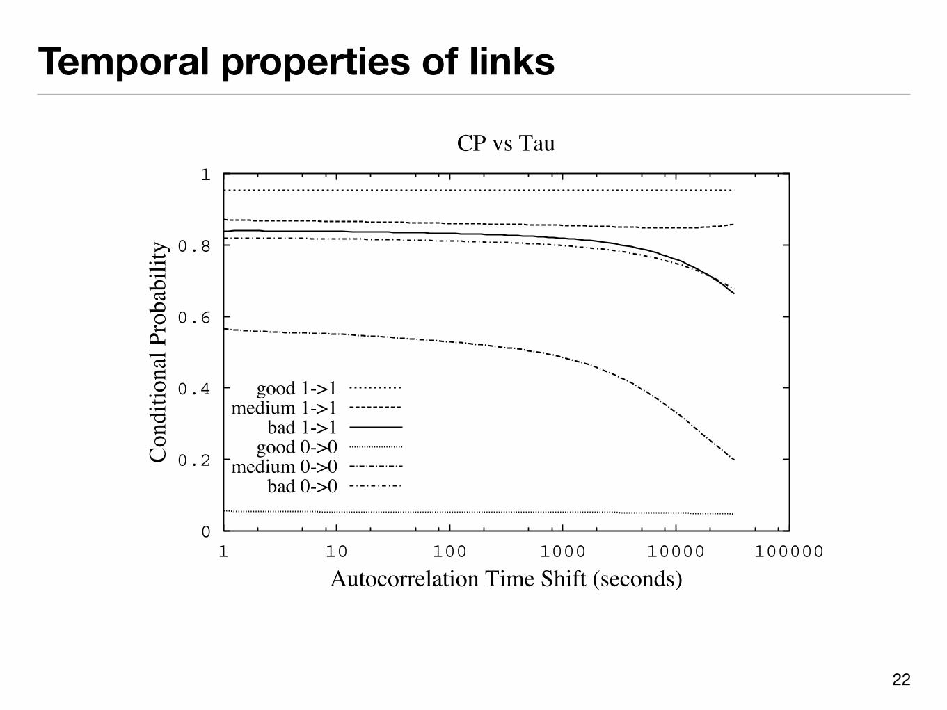
Temporal properties of links
22
0 1 2 3 40
0.5
1
1.5
2
2.5
3
3.5
LOG(1/RR)
LOG
(RNP
)
(a) Links characterized by their 1/RR andRNP values
0 1 2 3 40
0.5
1
1.5
2
2.5
3
3.5
LOG(1/RR)
LOG
(RNP
)
12.5%25%50%75%85.2%
(b) CDF of RNP as function of 1/RR (doublelogarithmic scale)
Figure 4: RNP as a function of 1/RR.
0 0.98 1.98 2.98 3.98 0
4.43
9.10
13.76
0
0.05
0.1
0.15
0.2
0.25
Dista
nce (
m)
LOG(Expected # of Messages)
(a) RNP and link length PDF
0
0.2
0.4
0.6
0.8
1
1 10 100 1000 10000 100000
Con
ditio
nal P
roba
bilit
y
Autocorrelation Time Shift (seconds)
CP vs Tau
good 1->1medium 1->1
bad 1->1good 0->0
medium 0->0bad 0->0
(b) CP as a function of τ
Figure 5: RNP and Autocorrelation.
4.1 Single Link AutocorrelationThe most common measure for the quality of links is the
percentage of received packets over a certain period of time,reception rate (RR). We will see that a better measure is toconsider the average number of packets that must be sentbefore a packet is received. We will refer to this value asthe required number of packets (RNP). Commonly, it is as-sumed there is a reverse relationship between RNP and RR.However, temporal correlations often invalidates this.
For example, consider the four links shown in Figures 2and 3. In this case, we show the aggregated reception rate(by minute) of the data from set B. In Figure 2(a) we see alink with an average reception rate of 48.02%. This link ishighly unreliable and the required number of packets (withconstant back-off) will be high (1189.65), even though thereare minutes where the link is reliable. In Figure 2(b)) weshow a link that has very high reception rate (95.36%). Inthis case, while a few messages were not received the linkwas completely reliable with very low required number ofpackets (1.05). Consider the medium quality links shown inFigures 3(a) and 3(b). The first link has a RR of 86.39%
and the second link has a RR of 79.86%. When using RRas a quality metric, clearly the first link is better than thesecond. Surprisingly, when using RNP, the second link ismuch better than the first. The reason of this counterintu-itive result is due to the fact that the RR metric does nottake into account the underlying distribution of the losses;short periods of zero RR in any particular time interval willtrigger the RNP to higher values, even though the averageRR might still be higher than the other link in the sametime interval. As a result of this inconsistent behavior, therequired number of packets provides a better picture of theusefulness of the link.
We statistically analyze the relationship between the re-ception rate and the required number of packets using datasets B and D to fully characterize the usefulness of moderatelinks. Figure 4 shows the relationship between RNP and RRin log scale. If the underlying distribution of packet lossescorresponds to a random uniform distribution, we would ex-pect a one-to-one relationship between RNP and RR. Fromthe figure we clearly see this is not the case. Perhaps moreimportantly, using RR as the main evaluation of link quality
417

Temporal properties of links• Good and bad links are temporally stable• Intermediary links have significant fluctuations
23

Next class• Low-power MACs
24


