fibers

Article

Probabilistic Seismic Demand Analysis of a Bridgewith Unbonded, Post-Tensioned, Concrete-Filled,Fiber-Reinforced Polymer Tube Columns

Manisha Rai 1, Mohamed A. ElGawady 2,* and Adrian Rodriguez-Marek 3

1 Guidewire Cyence Risk Analytics, San Mateo, CA 94401, USA; mrai@guidewire.edu2 Civil, Arch. and Environmental Eng. Dept., Missouri University S&T, Rolla, MO 65401, USA3 The Charles E. Via, Jr. Department of Civil and Environmental Engineering, Virginia Tech., Blacksburg,

VA 24060, USA; adrianrm@vt.edu* Correspondence: elgawadym@mst.edu; Tel.: +1-573-308-7358

Received: 17 September 2018; Accepted: 5 March 2019; Published: 18 March 2019�����������������

Abstract: Ground motions at sites close to a fault are sometimes affected by forward directivity, wherethe rupture energy arrives at the site in a form of a very short duration pulse. These pulses impose aheavy demand on structures located in the vicinity of the fault. In this research, a probabilistic seismicdemand analysis (PSDA) for a self-centering bridge is carried out. The bridge columns consistedof unbonded, post-tensioned, concrete-filled, fiber-reinforced polymer tubes. A bridge model wasdeveloped and non-linear time history analyses were performed. Three different methodologies thatused spectral accelerations to predict structural responses were used, and a time-domain approachwas used for PSDA. In addition to the three approaches, a time-domain PSDA methodology was alsoused. The results of the PSDA from the four approaches are compared, and the advantages of usingthe time-domain methodology are discussed. The results of the PSDA showed that for a site locatedvery close to the fault (6 km in this study), earthquakes having a magnitude (Mw) as small as 6.5 canbe significantly hazardous because the periods of pulses generated by small magnitude earthquakescoincide with the periods of the bridge. Since small magnitude events occur with greater frequencythan large magnitude events, they can have important contributions to risk.

Keywords: probabilistic seismic demand analysis; concrete bridges; failures; structural design

1. Introduction

Current practices in the seismic design of structures involves the determination of earthquakeloads using seismic hazard analysis, which is commonly performed within the framework ofprobabilistic seismic hazard analysis (PSHA), and then these loads for structural design are usedwithin the design framework dictated by building codes [1]. The output of a PSHA is mean annualrates of exceedance curves for intensity measures (IM) of ground motion. The designer then selectsan acceptable level of risk by selecting a return period of the IM. An alternative approach is to useperformance-based seismic design (PBSD), which refers to a framework that allows for structuraland non-structural design decisions to be made in terms of the mean annual rate of exceedance ofdecision variables (DV) such as dollar value of loss, death toll due to collapse, or downtime underdifferent seismic demands. PBSD accounts for all sources of uncertainty in computing exceedancecurves for the DV. These computations involve, among other steps, the computation of the meanannual rate of exceedance of parameters that characterize structural response through engineeringdemand parameters (EDPs). The computation of these exceedance rates is known as probabilisticseismic demand analysis (PSDA) [1].

Fibers 2019, 7, 23; doi:10.3390/fib7030023 www.mdpi.com/journal/fibers

Fibers 2019, 7, 23 2 of 23

In this paper, PSDA was applied to a self-centering bridge that was affected by near-fault groundmotions. This problem is of particular interest since there is a strong momentum around the worldto develop self-centering bridge systems; however, the behavior of self-centering bridges underpulse-type loading has not been studied. The methodology presented in this paper uses a traditionalPSHA methodology for computing structural responses for ordinary ground motions. Furthermore,the paper introduces a time-domain methodology for computing structural responses of the bridge tothe pulse-like ground motions resulting from forward directivity effects.

The paper starts by presenting background information on PSDA, self-centering bridges, andnear-fault ground motion. The model used for structural analysis of the bridge is then described,followed by a description of the PSDA approach adopted for this study. Results are then discussedin terms of the improvement in structural predictions brought upon by the use of the time-domainPSDA approach.

2. Background

Forward directivity (FD) occurs when the fault rupture propagates towards the site at a velocitynearly equal to the shear wave velocity; these effects are observed at sites that are located in thedirection of rupture propagation. Ground motions affected by FD are different from those recorded farfrom the fault [2]. In FD ground motions, the energy from the fault rupture arrives at the near-fault sitein the form of one or more large pulses, which results in a large seismic demand on a structure [3–12].Near-fault pulse-like ground motions have both higher IM levels than non-pulse ground motions andproduce higher responses for the same IM level compared to non-pulse ground motions [2,13–16].

2.1. Pereformance-Based Seismic Design

PSDA involves the convolution of the hazard curve for an IM with the fragility curve, whichpredicts structural responses through EDP in terms of the selected IM. This is expressed as:

λEDP =∫

P(EDP > x|IM)|dλ(IM)|, (1)

where the term dλ is the slope of the mean annual rate of exceedance curve (e.g., the hazard curve) ofthe IM, and the term P(EDP > x|IM) is the conditional probability of exceeding a given EDP level for agiven IM (e.g., the fragility curve).

Recently, Sehhati et al. [16] proposed a methodology to account for near-fault effects in the PSDAanalysis of multi-story steel frame buildings. They showed that for multi-story structures, the EDPsresulting from ground motions having forward directivity are similar to those resulting from Gaborwavelet pulses when 0.50 < Tp/T1 < 2.5, where T1 is the fundamental period of the structure and Tp isthe pulse period. Within this range of periods, the structure under consideration could be analyzedusing simple pulses, which significantly reduces the analysis cost and time.

2.2. Self-Centering Bridges

Under the prevailing capacity design concepts, correctly designed and detailed reinforced concrete(RC) structures are anticipated to exhibit an inelastic response, damage, and permanent drifts at theconclusion of ground motion excitation. These damages require expensive repairs, or even completereplacements, leading to long-term closures of highways.

Research has shown that implementing a self-centering system using an unbonded,post-tensioning, precast construction system can minimize residual displacement and damage toconcrete structures as a result of seismic loads [17]. The inelastic deformations are accommodatedwithin the connection itself where a controlled rocking motion occurs (from the opening and closing ofthe existing gap). Using this concept, the structural element remains elastic with limited damage [18].

A few researchers have investigated the seismic response of segmental precast post-tensioned(PPT) columns [19–21]. Tests showed that PPT segmental columns were capable of undergoing

Fibers 2019, 7, 23 3 of 23

large nonlinear displacements without experiencing significant or sudden losses of strength.The nonlinearity resulted from the opening of the gaps between segments rather than materialnonlinearity, leading to limited hysteretic energy dissipation. Furthermore, residual displacementsand damages were smaller than those corresponding to typical monolithic RC columns. Increasingthe post-tensioning force significantly reduced the residual displacement but led to more concretecrushing [22]. Furthermore, to minimize concrete local damage, concrete-filled, fiber-reinforcedpolymer (FRP) tubes (CFFT) were used. CFFTs is an emerging system for both monolithic and rockingcolumns [23,24].

This study uses the PSDA framework recently proposed by Sehhati et al. [16] to determine theseismic demand on a self-centering concrete bridge located in the near-fault region and subjectedto potential FD effects. The results from this PSDA were compared to those from more traditionalapproaches used to carry out the PSDA analysis for near-fault sites.

3. Bridge Prototype and Modeling

A bridge having general geometric characteristics similar to those used in the NCHRP Project12-49 [25] was adopted (Figure 1). The bridge had five equal spans of 30.5 m each, with fourintermediate bents of 9.8 m, 14.8 m, 16.4 m, and 14.8 m heights, respectively. The superstructure was acast-in-place concrete box girder with three cells. The RC columns of the bridge in the NCHRP Project12-49 had a diameter of 1.17 m. For this study, these columns were replaced by precast post-tensionedconcrete-filled fiber tube (PPT-CFFT) piers which have self-centering capabilities [26–28]. In order tocome up with PPT-CFFT columns comparable in strength and stiffness to those in the original design,the dimensions of the new column were selected identical to those of the original columns (Figure 2).The chosen FRP had an elastic modulus and tensile strength of 1.5 GPa and 234 MPa, respectively, inthe hoop direction. The FRP tube thickness was taken as 15.4 mm. Grade 160 unbonded post-tensionedsteel bars were used. An initial post-tensioning force corresponding to a value of 45% of concretecompressive strength (f’

c) was found to give an initial yield moment and ultimate moment capacityvery similar to that of the RC section in the original design. Initial steel stress of 60% of the rebar yieldstress was selected, based on the recommendation in the literature [27,28].Fibers 2018, 6, x FOR PEER REVIEW 4 of 23

Figure 1. Bridge structure. (a) Plan and (b) Elevation (reproduced from Zhu et al. [27]).

Figure 2. Column cross-section.

Figure 1. Bridge structure. (a) Plan and (b) Elevation (reproduced from Zhu et al. [27]).

Fibers 2019, 7, 23 4 of 23

Fibers 2018, 6, x FOR PEER REVIEW 4 of 23

Figure 1. Bridge structure. (a) Plan and (b) Elevation (reproduced from Zhu et al. [27]).

Figure 2. Column cross-section. Figure 2. Column cross-section.

A three-dimensional spine bridge model was developed in SAP2000 (Figure 3a). The bridgesuperstructure was modeled using elastic beam elements passing through the centroid of thesuperstructure. A cross girder at each bent was modeled using beam elements located at the centroidof the box girder (Figure 3b). A rigid beam element was used to connect the top of the column to thecross girder [29]. The columns were modeled using beam elements located at the geometric center ofeach column. Rigid moment connections were used between each column and its foundation, as wellas between each column and the corresponding link that was connected to the superstructure. Plastichinges were selected at the top and bottom ends of each column (Figure 4). The girder had a dead loadof 60 kN/m. Additional dead loads included two-end diaphragms, 525 kN each, five intermediatediaphragms, 68 kN each, and four intermediate cross beams of 454 kN.

Fibers 2018, 6, x FOR PEER REVIEW 5 of 23

(a)

(b)

Figure 3. Bridge model: (a) entire bridge structure and (b) pier frame (reproduced from Zhu et al. [27]).

Figure 3. Cont.

Fibers 2019, 7, 23 5 of 23

Fibers 2018, 6, x FOR PEER REVIEW 5 of 23

(a)

(b)

Figure 3. Bridge model: (a) entire bridge structure and (b) pier frame (reproduced from Zhu et al. [27]).

Figure 3. Bridge model: (a) entire bridge structure and (b) pier frame (reproduced from Zhu et al. [27]).Fibers 2018, 6, x FOR PEER REVIEW 6 of 23

Figure 4. SAP2000 model of the bridge.

Figure 5. A comparison of the moment-curvature plot of a concrete-filled, fiber-reinforced polymer tube (FRP-CFFT) column (at an initial concrete compression stress of 45% f’c) with a reinforced concrete (RC) column reproduced from Zhu et al. [27].

In order to calibrate the nonlinear behavior of the FRP-CFFT columns, pushover analyses were performed using SAP 2000 on columns identical to those used in the bridge model. The columns had heights of 9.1 m, 13.7 m, and 15.2 m. Each column was subjected to an initial axial load value of 3118 kN. The pushover curves were calculated using the Hewes and Priestley [28] model (Figure 6). The calibrated model of the bridge was then used for the non-linear time history analyses explained later in this paper.

Figure 4. SAP2000 model of the bridge.

The moment curvature relation along with the axial-force-moment interaction diagram was usedto define the plastic hinges. Moment curvature of an unbonded, post-tensioned column is inherentlydifferent from conventional RC columns. Hewes and Priestley [30] used an iterative model to calculatethe moment-curvature and backbone relationships for an unbonded, post-tensioned column. Asimilar procedure was used in this paper to determine the moment-curvature of the unbounded,post-tensioned column. The unconfined concrete compressive strength was considered as 27.6 MPa.The confined concrete was modeled using the Samaan et al. [31] model. Grade 160 steel rebar wasused for the post-tensioning tendons. The steel had an elastic modulus of 204,774 MPa, a yield stressof 874 MPa, an ultimate stress of 1109 MPa, and an ultimate strain of 10%.

Fibers 2019, 7, 23 6 of 23

The moment curvature analysis was carried out for a given post-tensioning force and differentvalues of applied axial loads. Since there was no clear yielding point for unbonded, post-tensionedcolumns, a bilinear idealization was used using equal energy concepts. The onset of the post-elasticpoint was considered as the yielding point. Finally, an axial load-moment interaction diagram wasdeveloped and was used as an input in SAP2000 (Figure 5).

Fibers 2018, 6, x FOR PEER REVIEW 6 of 23

Figure 4. SAP2000 model of the bridge.

Figure 5. A comparison of the moment-curvature plot of a concrete-filled, fiber-reinforced polymer tube (FRP-CFFT) column (at an initial concrete compression stress of 45% f’c) with a reinforced concrete (RC) column reproduced from Zhu et al. [27].

In order to calibrate the nonlinear behavior of the FRP-CFFT columns, pushover analyses were performed using SAP 2000 on columns identical to those used in the bridge model. The columns had heights of 9.1 m, 13.7 m, and 15.2 m. Each column was subjected to an initial axial load value of 3118 kN. The pushover curves were calculated using the Hewes and Priestley [28] model (Figure 6). The calibrated model of the bridge was then used for the non-linear time history analyses explained later in this paper.

Figure 5. A comparison of the moment-curvature plot of a concrete-filled, fiber-reinforced polymertube (FRP-CFFT) column (at an initial concrete compression stress of 45% f’

c) with a reinforced concrete(RC) column reproduced from Zhu et al. [27].

In order to calibrate the nonlinear behavior of the FRP-CFFT columns, pushover analyses wereperformed using SAP 2000 on columns identical to those used in the bridge model. The columns hadheights of 9.1 m, 13.7 m, and 15.2 m. Each column was subjected to an initial axial load value of 3118 kN.The pushover curves were calculated using the Hewes and Priestley [28] model (Figure 6). The calibratedmodel of the bridge was then used for the non-linear time history analyses explained later in this paper.Fibers 2018, 6, x FOR PEER REVIEW 7 of 23

Figure 6. Comparison of pushover curves from SAP2000 and from Hewes and Priestly [28] model for the three columns after calibration.

4. Ground Motions and Fault Geometry

For the non-linear time history analyses of the bridge, the ground motions were extracted from a database compiled by Sehhati et al. (2011) that included a set of 27 FD and 27 non-forward directivity (NFD) ground motions. Each ground motion was recorded for earthquakes with moment magnitudes (Mw) greater than 6.5 and at a source-to-site distance (R) less than 20 km. Only the fault-normal components of these records were used and applied to the bridge in the weak/transverse direction. It was assumed that the weak axis of the bridge was perpendicular to the fault. The maximum bridge drift at the top of the bridge column was selected as the EDP.

A hypothetical vertical strike-slip fault of 240 km length was considered. For simplicity of calculation, it was assumed that the fault was a straight line and the seismicity rate was 1. The earthquake magnitude distribution was assumed to follow a bounded Gutenberg–Richter recurrence law with a beta value of 1.84 (or b = 0.8) and with bounding magnitudes of 5.0 and 8.0. In the Gutenberg–Richter law, the probability of exceedance of any given magnitude decreases exponentially with the magnitude. The longitudinal direction of the bridge was assumed to be parallel to the fault longitudinal axis, as shown in Figure 7. Four different fault-site distances (6, 11, 16, and 21 km) were considered in the analyses to investigate the effects of source-to-site distance on the analysis. For each location of the bridge, four different approaches were used for the PSDA.

Figure 6. Comparison of pushover curves from SAP2000 and from Hewes and Priestly [28] model forthe three columns after calibration.

Fibers 2019, 7, 23 7 of 23

4. Ground Motions and Fault Geometry

For the non-linear time history analyses of the bridge, the ground motions were extracted from adatabase compiled by Sehhati et al. (2011) that included a set of 27 FD and 27 non-forward directivity(NFD) ground motions. Each ground motion was recorded for earthquakes with moment magnitudes(Mw) greater than 6.5 and at a source-to-site distance (R) less than 20 km. Only the fault-normalcomponents of these records were used and applied to the bridge in the weak/transverse direction. Itwas assumed that the weak axis of the bridge was perpendicular to the fault. The maximum bridgedrift at the top of the bridge column was selected as the EDP.

A hypothetical vertical strike-slip fault of 240 km length was considered. For simplicity ofcalculation, it was assumed that the fault was a straight line and the seismicity rate was 1. Theearthquake magnitude distribution was assumed to follow a bounded Gutenberg–Richter recurrencelaw with a beta value of 1.84 (or b = 0.8) and with bounding magnitudes of 5.0 and 8.0. In theGutenberg–Richter law, the probability of exceedance of any given magnitude decreases exponentiallywith the magnitude. The longitudinal direction of the bridge was assumed to be parallel to the faultlongitudinal axis, as shown in Figure 7. Four different fault-site distances (6, 11, 16, and 21 km) wereconsidered in the analyses to investigate the effects of source-to-site distance on the analysis. For eachlocation of the bridge, four different approaches were used for the PSDA.

Fibers 2018, 6, x FOR PEER REVIEW 7 of 23

Figure 6. Comparison of pushover curves from SAP2000 and from Hewes and Priestly [28] model for the three columns after calibration.

4. Ground Motions and Fault Geometry

For the non-linear time history analyses of the bridge, the ground motions were extracted from a database compiled by Sehhati et al. (2011) that included a set of 27 FD and 27 non-forward directivity (NFD) ground motions. Each ground motion was recorded for earthquakes with moment magnitudes (Mw) greater than 6.5 and at a source-to-site distance (R) less than 20 km. Only the fault-normal components of these records were used and applied to the bridge in the weak/transverse direction. It was assumed that the weak axis of the bridge was perpendicular to the fault. The maximum bridge drift at the top of the bridge column was selected as the EDP.

A hypothetical vertical strike-slip fault of 240 km length was considered. For simplicity of calculation, it was assumed that the fault was a straight line and the seismicity rate was 1. The earthquake magnitude distribution was assumed to follow a bounded Gutenberg–Richter recurrence law with a beta value of 1.84 (or b = 0.8) and with bounding magnitudes of 5.0 and 8.0. In the Gutenberg–Richter law, the probability of exceedance of any given magnitude decreases exponentially with the magnitude. The longitudinal direction of the bridge was assumed to be parallel to the fault longitudinal axis, as shown in Figure 7. Four different fault-site distances (6, 11, 16, and 21 km) were considered in the analyses to investigate the effects of source-to-site distance on the analysis. For each location of the bridge, four different approaches were used for the PSDA.

Figure 7. Fault geometry and bridge locations used in the study.

5. Probabilistic Seismic Demand Analysis (PSDA) Approaches

The PSDA computations used the annual rate of exceedance of one or more IMs to obtain theannual rate of exceedance of an EDP (λEDP). Four different approaches to compute PSDA for thebridge were used during the course of this study. These approaches can be split into two main broadgroups, namely, the conventional approach and the time-domain approach. In the ensuing, each ofthese approaches are discussed in detail.

5.1. Conventional PSDA Approach

The conventional PSDA is described by Equation (1). This equation requires the definition of thehazard curve for Sa, and the probability of exceeding an EDP value for a given Sa. In this study, threedifferent approaches to obtain these two functions were applied:

I. The traditional PSDA approach, in which the near-fault directivity effects were purposelyignored. This analysis was conducted as a baseline case for comparison with cases in which near-faulteffects were accounted for. The Abrahamson and Silva [32] ground motion prediction equation (GMPE)was used in this study for predicting the Sa. Note that while this GMPE has been largely supersededby more recent GMPEs, the choice of GMPE does not affect the comparison exercise conducted inthis paper. The EDP was formulated using a statistical relationship between EDP and IM, obtainedusing results of non-linear time history analyses of the bridge for near-fault and ordinary (i.e., withoutdirectivity effects) ground motions.

Fibers 2019, 7, 23 8 of 23

II. The broadband PSDA approach, in which near-fault directivity effects were accountedfor by using a modified GMPE. This study used the modified attenuation models developed bySomerville et al. [2] and Abrahamson [33]. This approach was called the Broadband approach becausethe selected GMPEs amplified the Sa predictions for near-fault sites in a wide range (i.e., broadband)of periods. The Broadband approach accounted for the effect of near-fault pulses on the IM observedat the site, but it ignored the effect of pulses on EDP for a given IM level.

III. The enhanced broadband approach in which the same GMPE as in the broadband case wasused, but the effects of near-fault directivity on EDP were also accounted for. The enhanced broadbandapproach used different predictive equations for EDP (as a function of IM) for cases when directivityeffects were observed and when they were not observed.

5.2. Time-Domain PSDA Approach

The time-domain approach proposed by Sehhati et al. [16] extends the enhanced broadbandapproach by directly using the results of time-domain analyses along with a vector of IMs. Theessence of this approach is that for cases when ground motions have pulses, the EDP is predictedusing simplified wavelet pulses instead of a correlation with IM. The parameters that characterizethe pulse motions are the amplitude and period of the pulse. For this purpose, ground motionscenarios were divided into four cases: non-near-source (non-NS), near-source no pulse (NS-NP),near-source pulse-dominant (NS-P-in), and near-source pulse-non-dominant (NS-P-out). Thenear-source pulse-dominant case refers to the case when the pulse in the near-source ground motiondrives the structural response. This occurs when the period of pulse in the ground motion is withina certain range of the structural period [16], thus, the EDP of the structure can be predicted using avector IM (e.g., pulse amplitude, Ap, and pulse period, Tp) and time domain analyses using wavelets.The near-source pulse-non-dominant case refers to scenarios where directivity effects are observed atthe site, but the period of the resultant pulse is very different from the period of the structure. In thesescenarios, an EDP–IM relationship for forward-directivity ground motions is used for EDP prediction.

6. Models Required for PSDA

The PSDA methodology that was developed by Sehhati et al. [16] was used in this study. Thebroadband, enhanced broadband, and time-domain approaches divided the hazard scenarios intoforward directivity and non-forward directivity cases; hence, the probability of observing forwarddirectivity ground motion at a given site, due to a given fault scenario, is required to carry out thePSDA. The model proposed by Iervolino and Cornell [34] was used to predict the probability ofobserving forward directivity at a given site from a given fault scenario.

To carry out the time-domain PSDA, it was required to determine the pulse amplitude (Ap) andpulse period (Tp) at a given site. This study predicted pulse amplitude as a function of peak groundvelocity (PGV) from the Bray and Rodriguez-Marek [35] model for distances less than 20 km fromthe fault. For distances greater than 60 km, a model developed by Abrahamson and Silva [32] wasused to predict PGV, and subsequently, pulse amplitudes. For intermediate distances (i.e., between20 to 60 km), a taper was used to transition between the two models [16]. The Baker [36] model wasused to predict the pulse period, Tp.

6.1. Engineering Demand Parameter–Intensity Measure (EDP–IM) Relationship for Forward Directivity (FD)and Non-Forward Directivity (NFD) Ground Motions

The EDP–Sa relationship for both pulse-like and non-pulse-like ground motion was needed forthe enhanced broadband approach. The maximum column drift angle resulting from non-linear timehistory analyses of the bridge structure for FD and NFD ground motions were plotted in Figure 8 asa function of the spectral acceleration of the input ground motion at the fundamental period of thebridge, Sa(T1). A power-law relationship was used and a least-square regression was employed to fit

Fibers 2019, 7, 23 9 of 23

a curve that represented the median of the maximum column drift for a given Sa. Equation (2) showsthe developed relationship:

Max.Column Dri f t (%) ==

{1.0749 (Sa(T1))

0.76, f or FD0.8597 (Sa(T1))

0.69, f or NFD, (2)

with standard deviations of the residuals, σln, valued at 0.27 and 0.25 for FD and NFD, respectively. Asshown in Figure 8, the medians of the maximum drifts for FD ground motions were higher than thoseof NFD ground motions for a given Sa. This occurred because pulses induced higher nonlinearities inthe bridge, resulting in a higher structural demand.

Fibers 2018, 6, x FOR PEER REVIEW 9 of 23

The PSDA methodology that was developed by Sehhati et al. [16] was used in this study. The broadband, enhanced broadband, and time-domain approaches divided the hazard scenarios into forward directivity and non-forward directivity cases; hence, the probability of observing forward directivity ground motion at a given site, due to a given fault scenario, is required to carry out the PSDA. The model proposed by Iervolino and Cornell [34] was used to predict the probability of observing forward directivity at a given site from a given fault scenario.

To carry out the time-domain PSDA, it was required to determine the pulse amplitude (Ap) and pulse period (Tp) at a given site. This study predicted pulse amplitude as a function of peak ground velocity (PGV) from the Bray and Rodriguez-Marek [35] model for distances less than 20 km from the fault. For distances greater than 60 km, a model developed by Abrahamson and Silva [32] was used to predict PGV, and subsequently, pulse amplitudes. For intermediate distances (i.e., between 20 to 60 km), a taper was used to transition between the two models [16]. The Baker [36] model was used to predict the pulse period, Tp.

6.1. Engineering Demand Parameter–Intensity Measure (EDP–IM) Relationship for Forward Directivity (FD) and Non-Forward Directivity (NFD) Ground Motions

The 𝐸𝐷𝑃–𝑆 relationship for both pulse-like and non-pulse-like ground motion was needed for the enhanced broadband approach. The maximum column drift angle resulting from non-linear time history analyses of the bridge structure for FD and NFD ground motions were plotted in Figure 8 as a function of the spectral acceleration of the input ground motion at the fundamental period of the bridge, 𝑆 (𝑇 ). A power-law relationship was used and a least-square regression was employed to fit a curve that represented the median of the maximum column drift for a given 𝑆 . Equation (2) shows the developed relationship: 𝑀𝑎𝑥. 𝐶𝑜𝑙𝑢𝑚𝑛 𝐷𝑟𝑖𝑓𝑡 (%) == 1.0749 (𝑆 (𝑇 )) . , 𝑓𝑜𝑟 𝐹𝐷0.8597 (𝑆 (𝑇 )) . , 𝑓𝑜𝑟 𝑁𝐹𝐷, (2)

with standard deviations of the residuals, 𝜎 , valued at 0.27 and 0.25 for FD and NFD, respectively. As shown in Figure 8, the medians of the maximum drifts for FD ground motions were higher than those of NFD ground motions for a given 𝑆 . This occurred because pulses induced higher nonlinearities in the bridge, resulting in a higher structural demand.

Figure 8. Plots of bridge responses to forward directivity (FD) and non-forward directivity (NFD)ground motions.

6.2. EDP Versus Pulse Parameter Relationship for Simplified Pulses

A relationship between EDP and pulse parameters (Ap, Tp) was required for the time-domainapproach. Sehhati et al. [16] showed that for cases when ground motion pulses dominate structuralresponse, a simplified wavelet pulse could be used to capture the response of a structure to the pulsemotions. Similarly, in this study Gabor pulses were used to capture the response of the bridge structureto pulse-like motions. The velocity time history of a Gabor pulse is given by the following equation [36]:

V(t) =

{A 1

2

[1 + cos

(2π fp

γ (t− t0))]

cos[2π fp(t− t0) + v

], t0 − γ

2 fp≤ t ≤ to +

γ2 fp

0, Otherwise(3)

where, A is proportional to the amplitude of the wavelet, fp is the prevailing frequency of the signal, ν isthe phase angle (i.e., ν = 0 and ν = ±π/2, defining symmetric and anti-symmetric signals, respectively),γ defines the oscillatory character of the signal, and to is the time of the envelope’s peak. In this study,only ν = 0 had been considered, for simplicity. Hence, the only parameters that were required to definethe Gabor wavelet pulse were A, fp, and γ. The Baker [36] procedure was used to extract the pulsefrom FD ground motion, and based on the number of peaks and troughs of the extracted pulses, theparameter γ was set as 3.

Fibers 2019, 7, 23 10 of 23

Time history analyses of the bridge model were carried out under the effects of different Gaborpulses and forward-directivity ground motions. Figure 9 shows a ratio of computed EDP values (inthis case, the maximum column drift angle) for the recorded forward-directivity ground motions andfor equivalent pulses. Sehhati et al. [16] observed that for multi-degree-of-freedom structures, theresponses to the FD ground motions were equal to the responses to equivalent simplified pulses (i.e.,ratio = 1) when 0.5 < Tp/T1 < 2.5 for multi-degree-of-freedom structures. For the bridge under study,this was the case for Tp/T1 < 1.75. For the lower limit on Tp/T1, the lower limit of 0.5 was adoptedfrom Sehhati et al. [16]. Nonlinear time-history analyses were performed in SAP2000 using simplifiedGabor pulses for this range of pulse period and for a range of pulse amplitudes (15 < Ap ( cm

s ) < 60).Maximum bridge drifts and base shear forces were monitored for all pulses; however, only the formerwas considered as the EDP. A genetic algorithm (Schmidt and Lipson, 2009) was used to perform asymbolic regression to find the functional form for the maximum drift. The surface (Figure 10) for themaximum column drift had the following functional form:

Max Dri f t(%) =5.03073 + Ap

( 127.58sin(0.0602+Tp)

− 175.35 cos(Tp))

(4)

Fibers 2018, 6, x FOR PEER REVIEW 11 of 23

Figure 9. Plot showing the ratios of EDP computed for recorded ground motions to those computed using equivalent pulses, plotted against 𝑇 𝑇⁄ .

Figure 10. The EDP response surface of the bridge to simplified Gabor pulses.

7. Results and Discussion

The results of the PSDA for four different site locations at 6 km, 11 km, 16 km, and 21 km from the fault are shown in Figure 11. The results of the enhanced broadband approach and the individual contributions from its two components, namely the pulse and non-pulse motions, are shown. Note that the probability of exceedance (𝜆 ) of the non-pulse component was higher than those of the pulse component for small drift angles. However, 𝜆 for the non-pulse component decreased with increasing drift angles. The reason for this variation was as follows. Lower values of drift angle could

Figure 9. Plot showing the ratios of EDP computed for recorded ground motions to those computedusing equivalent pulses, plotted against Tp/T1

Fibers 2019, 7, 23 11 of 23

Fibers 2018, 6, x FOR PEER REVIEW 11 of 23

Figure 9. Plot showing the ratios of EDP computed for recorded ground motions to those computed using equivalent pulses, plotted against 𝑇 𝑇⁄ .

Figure 10. The EDP response surface of the bridge to simplified Gabor pulses.

7. Results and Discussion

The results of the PSDA for four different site locations at 6 km, 11 km, 16 km, and 21 km from the fault are shown in Figure 11. The results of the enhanced broadband approach and the individual contributions from its two components, namely the pulse and non-pulse motions, are shown. Note that the probability of exceedance (𝜆 ) of the non-pulse component was higher than those of the pulse component for small drift angles. However, 𝜆 for the non-pulse component decreased with increasing drift angles. The reason for this variation was as follows. Lower values of drift angle could

Figure 10. The EDP response surface of the bridge to simplified Gabor pulses.

7. Results and Discussion

The results of the PSDA for four different site locations at 6 km, 11 km, 16 km, and 21 km fromthe fault are shown in Figure 11. The results of the enhanced broadband approach and the individualcontributions from its two components, namely the pulse and non-pulse motions, are shown. Notethat the probability of exceedance (λEDP) of the non-pulse component was higher than those of thepulse component for small drift angles. However, λEDP for the non-pulse component decreased withincreasing drift angles. The reason for this variation was as follows. Lower values of drift angle couldbe exceeded with a high probability with lower magnitude ground motions (which occur much morefrequently compared to larger magnitude ground motions). The probability that a lower magnitudeearthquake will be in the form of a pulse was low. Hence, the overall probability that a smaller valueof drift angle was exceeded due to a pulse component also decreased. It is worth noting that theprobability of having a pulse depends on the distance between the point on the fault closest to thesite and the epicenter (R), the length of rupture (S), and the angle between the strike of the fault andthe line joining the epicenter to the site (θ or theta). Lower magnitude earthquakes have smallermedian fault rupture lengths; hence, they have a lower probability to be in the form of a pulse. Highvalues of drift angle would be exceeded only with larger magnitude earthquakes that have a higherprobability of having a pulse. However, such high magnitude ground motions have a lower probabilityof occurrence, resulting in a lower overall probability that a large drift angle is exceeded as a result of apulse or non-pulse component.

Figure 12 shows a comparison of the probability of exceedance calculated using all four PSDAmethodologies. For the site at 6 km (Figure 12a), all the methods yielded similar results for drift anglessmaller than 0.5%. Beyond that, the time-domain PSDA yielded higher values of λEDP comparedto the other three methodologies. This was because the time-domain approach captured resonancein a better way (by using Ap and Tp as intensity measures) as compared to other methodologiesand was, thus, able to better capture non-linearity at higher drift levels. In addition, beyond a driftangle of about 0.5%, the enhanced broadband PSDA yielded higher values of λEDP compared to thetraditional and broadband PSDA methodologies. This happened because at higher drift levels, amajor contribution to EDP exceedances came from the pulse-like component that was only captured

Fibers 2019, 7, 23 12 of 23

by the enhanced broadband approach. This implied that it was important to capture the differencesin structural responses to non-pulse-like and pulse-like motions (Figure 8). At progressively largerdistances from the fault (Figure 12b–d), trends similar to those discussed for the site at 6 km wereobserved. However, the probability of exceeding a particular drift angle became smaller comparedto those of a site at 6 km. Also, with increasing the distance between the epicenter and the site, thedifference in the probability of exceedance calculated using the new PSDA and enhanced broadbandkept decreasing, indicating the reduction in contribution of pulse-in components at this distance.

Fibers 2018, 6, x FOR PEER REVIEW 12 of 23

be exceeded with a high probability with lower magnitude ground motions (which occur much more frequently compared to larger magnitude ground motions). The probability that a lower magnitude earthquake will be in the form of a pulse was low. Hence, the overall probability that a smaller value of drift angle was exceeded due to a pulse component also decreased. It is worth noting that the probability of having a pulse depends on the distance between the point on the fault closest to the site and the epicenter (R), the length of rupture (S), and the angle between the strike of the fault and the line joining the epicenter to the site (θ or theta). Lower magnitude earthquakes have smaller median fault rupture lengths; hence, they have a lower probability to be in the form of a pulse. High values of drift angle would be exceeded only with larger magnitude earthquakes that have a higher probability of having a pulse. However, such high magnitude ground motions have a lower probability of occurrence, resulting in a lower overall probability that a large drift angle is exceeded as a result of a pulse or non-pulse component.

Figure 11. Rate of exceedance of drift vs. maximum drifts from the enhanced broadband approach, and the individual contributions of pulse and non-pulse motions are shown for sites located at a distance of (a) 6 m, (b) 11 km, (c) 16 km, and (d) 21 km from the fault.

Figure 11. Rate of exceedance of drift vs. maximum drifts from the enhanced broadband approach, andthe individual contributions of pulse and non-pulse motions are shown for sites located at a distance of(a) 6 m, (b) 11 km, (c) 16 km, and (d) 21 km from the fault.

Fibers 2019, 7, 23 13 of 23

Fibers 2018, 6, x FOR PEER REVIEW 13 of 23

Figure 12 shows a comparison of the probability of exceedance calculated using all four PSDA methodologies. For the site at 6 km (Figure 12a), all the methods yielded similar results for drift angles smaller than 0.5%. Beyond that, the time-domain PSDA yielded higher values of 𝜆 compared to the other three methodologies. This was because the time-domain approach captured resonance in a better way (by using Ap and Tp as intensity measures) as compared to other methodologies and was, thus, able to better capture non-linearity at higher drift levels. In addition, beyond a drift angle of about 0.5%, the enhanced broadband PSDA yielded higher values of 𝜆 compared to the traditional and broadband PSDA methodologies. This happened because at higher drift levels, a major contribution to EDP exceedances came from the pulse-like component that was only captured by the enhanced broadband approach. This implied that it was important to capture the differences in structural responses to non-pulse-like and pulse-like motions (Figure 8). At progressively larger distances from the fault (Figure 12b–d), trends similar to those discussed for the site at 6 km were observed. However, the probability of exceeding a particular drift angle became smaller compared to those of a site at 6 km. Also, with increasing the distance between the epicenter and the site, the difference in the probability of exceedance calculated using the new PSDA and enhanced broadband kept decreasing, indicating the reduction in contribution of pulse-in components at this distance.

Figure 12. Rate of exceedance of drift vs. maximum drifts from the four methods (traditional, broadband, enhanced broadband and time–domain method) are shown for sites located at a distance of (a) 6 m, (b) 11 km, (c) 16 km, and (d) 21 km from the fault.

Figure 12. Rate of exceedance of drift vs. maximum drifts from the four methods (traditional,broadband, enhanced broadband and time–domain method) are shown for sites located at a distanceof (a) 6 m, (b) 11 km, (c) 16 km, and (d) 21 km from the fault.

Figure 13 shows the results of the proposed time-domain PSDA. The contributions of four differentcontributors to total demand are also shown separately ((non-NS), (NS-NP), (NS-P-in), and (NS-P-out)).As in the case of Figure 9, for smaller drift angles, the NS-NP component had the highest probabilityof exceedance. For higher drift angles, most of the contribution to the hazard was coming from theNS-P-in scenario, pointing to the importance of such scenarios in the hazard calculations. As thedistance to the fault increased, the probability of exceeding a given drift angle decreased overall.

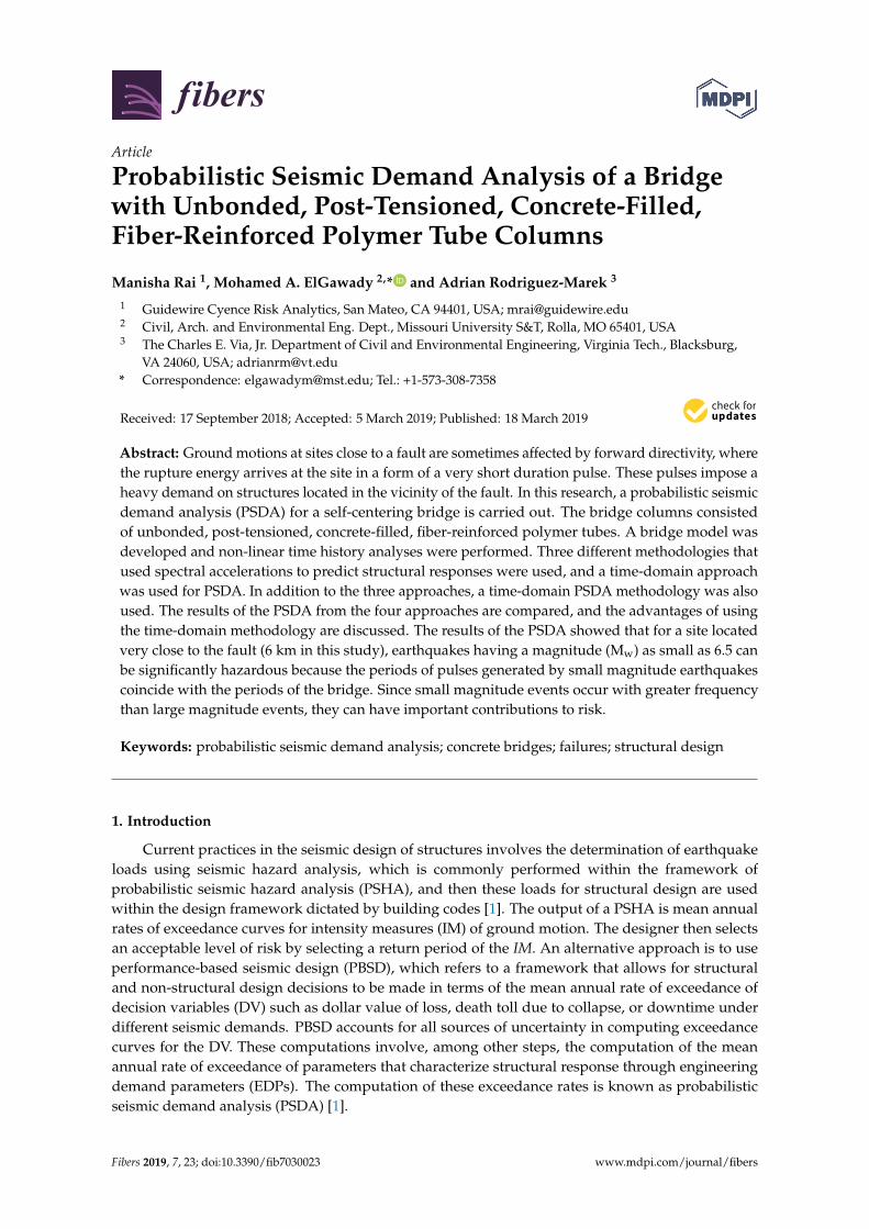
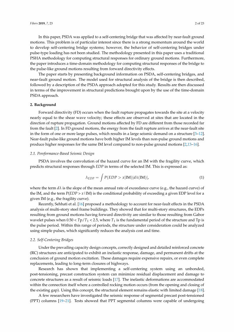
Figure 14 shows distance-magnitude deaggregation plots for a drift angle of 1% (which was anarbitrarily selected value for demonstration purposes). Figure 14a shows the distance-magnitudedeaggregation plots for a site located at a distance of 6 km from the fault. Contributions from differentcomponent of the New PSDA are shown. As expected, the main contribution to the hazard camefrom the near-source scenario. The NS-P-in component represented about 58% of total hazard, whichwas the highest contribution to the hazard. The next highest contributor to the total hazard was theNS-P-out component that represented 24% of the total hazard. The NS-NP contributed 18% to the totalhazard, making it the third highest contributor. The contribution from Non-NS was insignificant in

Fibers 2019, 7, 23 14 of 23

this case, and it represented 0.0% of the total hazard. The non-near source scenarios were the oneswith source-to-site distances greater than 60 km. Given the length and the location of the fault, and thelocation of the site, any fault rupture that was at a distance greater than 60 km from the site wouldhave a small fault rupture length, and would therefore result from a smaller magnitude earthquake.Since small magnitude earthquakes at a large distance would not be able to drive the drift of the bridgemore than 1%, no contributions from the non-near source scenario to the total hazard are seen.

Fibers 2018, 6, x FOR PEER REVIEW 14 of 23

Figure 13 shows the results of the proposed time-domain PSDA. The contributions of four different contributors to total demand are also shown separately ((non-NS), (NS-NP), (NS-P-in), and (NS-P-out)). As in the case of Figure 9, for smaller drift angles, the NS-NP component had the highest probability of exceedance. For higher drift angles, most of the contribution to the hazard was coming from the NS-P-in scenario, pointing to the importance of such scenarios in the hazard calculations. As the distance to the fault increased, the probability of exceeding a given drift angle decreased overall.

Figure 13. Rate of exceedance of drift vs. maximum drifts from the time-domain probabilistic seismic demand analysis (PSDA), and contributions from different components of the time-domain procedure are shown for sites located at a distance of (a) 6 m, (b) 11 km, (c) 16 km, and (d) 21 km from the fault. The labels for the components are: NS-P-in—Near-source pulse motions with pulses dominant; NS-P-out— near-source pulse motions with non-dominant pulses; NS-NP— near-source motions without pulses; and Non-NS—non-near source motions.

Figure 14 shows distance-magnitude deaggregation plots for a drift angle of 1% (which was an arbitrarily selected value for demonstration purposes). Figure 14a shows the distance-magnitude

Figure 13. Rate of exceedance of drift vs. maximum drifts from the time-domain probabilistic seismicdemand analysis (PSDA), and contributions from different components of the time-domain procedureare shown for sites located at a distance of (a) 6 m, (b) 11 km, (c) 16 km, and (d) 21 km from thefault. The labels for the components are: NS-P-in—Near-source pulse motions with pulses dominant;NS-P-out— near-source pulse motions with non-dominant pulses; NS-NP— near-source motionswithout pulses; and Non-NS—non-near source motions.

Fibers 2019, 7, 23 15 of 23Fibers 2018, 6, x FOR PEER REVIEW 16 of 23

(a)

(b)

Figure 14. Cont.

Fibers 2019, 7, 23 16 of 23Fibers 2018, 6, x FOR PEER REVIEW 17 of 23

(c)

(d)

Figure 14. Distance-magnitude deaggregation plots from the time-domain analyses at a drift of 1% for sites located at a distance of (a) 6 km, (b) 11 km, (c) 16 km, and (d) 21 km. Results are shown separately for the total hazard and for the different components of the time-domain analyses. The labels for the components are: NS-P-in—Near-source pulse motions with pulses dominant; NS-P-out— near-source pulse motions with non-dominant pulses; NS-NP—near-source motions without pulses; and Non-NS—non-near source motions. The value in parenthesis is the total contribution to hazard for each component.

Figure 16 shows the pulse amplitude deaggregation plots of the pulse-in component of the new PSDA. The figure illustrates the contribution of various amplitudes and periods of pulses to the NS-P-in component of the hazard. In Figure 16a, which is for a site located at a distance of 6 km from the

Figure 14. Distance-magnitude deaggregation plots from the time-domain analyses at a drift of 1%for sites located at a distance of (a) 6 km, (b) 11 km, (c) 16 km, and (d) 21 km. Results are shownseparately for the total hazard and for the different components of the time-domain analyses. Thelabels for the components are: NS-P-in—Near-source pulse motions with pulses dominant; NS-P-out—near-source pulse motions with non-dominant pulses; NS-NP—near-source motions without pulses;and Non-NS—non-near source motions. The value in parenthesis is the total contribution to hazard foreach component.

Fibers 2019, 7, 23 17 of 23

Another important feature in the graph for near-source motions with dominant pulses (NS-P-in)for 6 km was that the maximum contribution to demand was coming from low-magnitude earthquakesat smaller distances, as opposed to what was observed in the other deaggregation plots. The reasonfor this trend was that the lower magnitude earthquakes occurred with higher probabilities, and thepulses from these earthquakes led to a high probability of exceeding drifts of 1%. However, NS-P-outand NS-NP components of small ground motions had lower probabilities of exceeding a drift angleof 1%. Therefore, the total probability that this drift level was exceeded by an NS-P-out and NS-NPcomponent for a small magnitude earthquake was lower than for higher magnitude earthquakes. Inthe total hazard plot (Figure 14a), the maximum contributor was also the lower magnitude earthquakeat short distances. This highlights the importance of lower magnitude earthquakes for structureslocated in the proximity of a fault.

At a distance of 11 km (Figure 14b), the NS-P-in contributions were 46% of the total, lowerthan the value at 6 km, but still higher than all other components at this distance. As explainedearlier, the NS-P-in components of lower magnitude earthquakes contributed significantly to thehazard. However, the higher magnitude earthquakes were contributing more to the total hazard, asthe contribution of NS-P-out and the NS-NP components had increased compared to those calculatedat a distance of 6 km. As the distance between the source and the fault increased (Figure 14c,d), thecontribution of the NS-P-in components to the total hazard decreased. In addition, the contribution ofthe NS-NP component and higher magnitude earthquakes to the total hazard increased with increasingthe distance between the site and the fault.

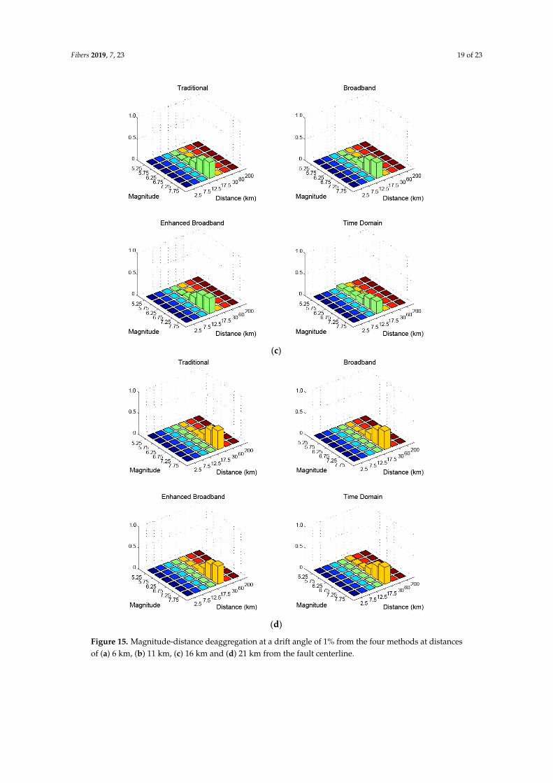
Figure 15 shows the distance-magnitude deaggregation plots for 1% drift level from the fourdifferent methods, mentioned earlier. At a site to fault distance of 6 km, the traditional, broadband, andenhanced broadband models followed the same trend, that higher magnitude earthquakes contributedmore to the total hazard; however, the new PSDA method showed that smaller magnitude earthquakescontributed more to the total hazard (Figure 15a). At a site-to-fault distance of 11 km, all the fourmodels showed that most of the hazard was due to higher magnitude earthquakes (Figure 15b).However, the new PSDA model showed that low-magnitude earthquakes significantly contributedto the total hazard, which differed from the other models. At site-to-fault distances of 16 and 21 km(Figure 15c,d), all four models showed that the largest contributions to the hazard came from largermagnitude earthquakes since low-magnitude earthquakes occurred at large distances from the bridge,resulting in small drift angles.

Figure 16 shows the pulse amplitude deaggregation plots of the pulse-in component of the newPSDA. The figure illustrates the contribution of various amplitudes and periods of pulses to theNS-P-in component of the hazard. In Figure 16a, which is for a site located at a distance of 6 km fromthe fault, it can be seen that the highest contribution was coming from the periods in the range of0.75 s and 1.00 s (centered at 0.875 s). This was because a structure was set into resonance wheneverthe pulse period was equal to the period of structure. The period of the bridge in the current studywas 0.8 s. Therefore, a pulse with this period would contribute the most to the NS-P-in componentof the hazard. Even though pulses with higher amplitudes induced larger drifts, the probabilitieswith which they occurred were lower, thus, their total contributions to the hazard were lower. Thiscontribution decreased further as distance to the fault increased (Figure 16b–d, due to the even smallerprobabilities of having these higher amplitude pulses in the ground motion). Thus, the contribution oflower amplitude pulses to the hazard increased.

Fibers 2019, 7, 23 18 of 23

Fibers 2019, 7, 23 18 of 23

fault, it can be seen that the highest contribution was coming from the periods in the range of 0.75 s and 1.00 s (centered at 0.875 s). This was because a structure was set into resonance whenever the pulse period was equal to the period of structure. The period of the bridge in the current study was 0.8 s. Therefore, a pulse with this period would contribute the most to the NS-P-in component of the hazard. Even though pulses with higher amplitudes induced larger drifts, the probabilities with which they occurred were lower, thus, their total contributions to the hazard were lower. This

(a)

(b)

Figure 15. Cont.

Fibers 2019, 7, 23 19 of 23

Fibers 2019, 7, 23 19 of 23

(c)

(d)

Figure 15. Magnitude-distance deaggregation at a drift angle of 1% from the four methods at distances of (a) 6 km, (b) 11 km, (c) 16 km and (d) 21 km from the fault centerline. Figure 15. Magnitude-distance deaggregation at a drift angle of 1% from the four methods at distancesof (a) 6 km, (b) 11 km, (c) 16 km and (d) 21 km from the fault centerline.

Fibers 2019, 7, 23 20 of 23

Fibers 2019, 7, 23 20 of 23

(a)

(b)

(c)

(d)

Figure 16. Period and amplitude deaggregation for a drift angle of 1% at a distance of (a) 6 km, (b) 11 km, (c) 16 km, and (d) 21 km from the centerline of the fault.

8. Conclusions

Figure 16. Period and amplitude deaggregation for a drift angle of 1% at a distance of (a) 6 km,(b) 11 km, (c) 16 km, and (d) 21 km from the centerline of the fault.

Fibers 2019, 7, 23 21 of 23

8. Conclusions

This paper presented a methodology for PSDA analysis for a self-centering bridge located in thenear-fault zone. An example is presented using a hypothetical fault in which analyses with differentdegrees of sophistication were conducted. The following conclusions were made:

• Pulse-like ground motions impose a heavy demand on the structure in the near-fault zone. Thishighlights the importance of properly considering these types of motions when designing bridgesin the near-fault region.

• The time-domain approach proposed by Sehhati et al. [16] has the advantage over other methodsof PSDA as it uses wavelet pulses to predict structural responses, which allows for the predictionof structural responses for all possible variations of pulse-parameters. This, in turn, permits thecapture of potential resonances in the bridge response. Moreover, structural nonlinearities areautomatically accounted for in time-domain analyses, whereas in using spectral accelerations,nonlinearities are only captured indirectly. The results of the time-domain analyses, thus, give abetter prediction of hazard for sites located in a near-fault region

• The results of the PSDA showed that for a site located very close to the fault (6 km in this study),small magnitude earthquakes can have significant contributions to structural demand. Thisobservation seems counter-intuitive at first since the results from all methodologies, other thanthe time-domain approach and conventional wisdom, point to the fact that large magnitudeevents should contribute most to the hazard. But, if the period of the bridge is closer to the periodof the pulses produced by small magnitude events than those produced by large magnitudeevents, the response of the bridge to small magnitude events may be comparable to the responseunder large magnitude events. A similar effect is discussed in Somerville [37]. Since the smallermagnitude events occur with greater frequency than larger magnitude events, they can havehigh contributions to the hazard. The possibility of contribution of small magnitude eventsto the hazard should be considered while selecting ground motions or while deciding thedesign scenarios.

• If a return period of 2475 years is considered, the drift values that were obtained from thetime-domain PSDA were more than 30% higher at short distances from the fault than thosefrom methodologies using spectral accelerations modified for near-fault effects. However, thisdifference reduces to about 15% at a distance of 11 km. This difference keeps getting smaller as thefault to site distance increases, and beyond distances of 16 km the difference is less than 5%, evenwith the high seismicity rate considered here. For more realistic seismicity rates, the differencewould be even lower (i.e., for the ground motion prediction models used in this study, the effectsof near-fault ground motion were insignificant for sites located more than 16 km from the fault).At such sites, more traditional methods using spectral accelerations as the intensity measure couldbe adopted for the hazard calculation instead of the more computationally expensive, proposedtime-domain analyses.

While this paper presents a comprehensive analysis of the probabilistic seismic hazard of a bridgedesigned using unbonded, post-tensioned, concrete-filled FRP tube columns, more case studies needto be investigated to develop a more comprehensive overview of these types of bridges. Parameterssuch as different span lengths, column heights, boundary conditions, soil-structure interaction, level ofpost-tension, etc., need to be carefully considered in the proposed case studies.

Author Contributions: The research idea was initiated by M.A.E. and A.R.-M., M.R. carried out the numericalanalyses and wrote the paper with close guidance, mentoring, and editing by M.A.E. and A.R.-M.

Funding: This research received no external funding.

Conflicts of Interest: The authors declare no conflict of interest.

Fibers 2019, 7, 23 22 of 23

Abbreviations

IM Intensity measuredλ Slope of the mean annual rate of exceedance curve (e.g., the hazard curve) of the IMEDP Engineering demand parameterP(EDP>x|IM) Conditional probability of exceeding a given EDP level for a given IMT1 Fundamental period of the structureTp Pulse periodAp Pulse amplitudeSa(T1) Fundamental period of the bridgeA A constant proportional to the amplitude of the waveletfp Prevailing frequency of the signalν Phase angleγ Defines the oscillatory character of the signalto Time of the envelope’s peak

References

1. SEAOC. Performance Based Seismic Engineering for Buildings (Vision 2000); Structural Engineers Association ofCalifornia: Sacramento, CA, USA, 1995.

2. Somerville, P.G.; Smith, N.F.; Graves, R.; Abrahamson, N.A. Modification of Empirical Strong GroundMotion Attenuation Relations to Include the Amplitude and Duration Effects of Rupture Directivity. Seismol.Res. Lett. 1997, 68, 199–222. [CrossRef]

3. Bertero, V.V.; Mahin, S.A.; Herrera, R.A. Aseismic design implications of near-fault San Fernando earthquakerecords. Earthq. Eng. Struct. Dyn. 1978, 6, 31–42. [CrossRef]

4. Anderson, J.C.; Bertero, V.V. Uncertainties in establishing design earthquakes. J. Struct. Eng. 1987, 113,1709–1724. [CrossRef]

5. Hall, J.F.; Heaton, T.H.; Halling, M.W.; Wald, D.J. Near-source ground motion and its effects on flexiblebuildings. Earthq. Spectra 1995, 11, 569–605. [CrossRef]

6. Iwan, W.; Huang, C.-T.; Guyader, A.C. Evaluation of the Effects of Near-Source Ground Motions; ReportDeveloped for the PG&E/PEER Program, CalTech: Pasadena, CA, USA, 1998.

7. Alavi, B.; Krawinkler, H. Effects of Near-Fault Ground Motions on Frame Structures; Dept. of Civil Eng., StanfordUniversity: Stanford, CA, USA, 2001.

8. Menun, C.; Fu, Q. An analytical model for near-fault ground motions and the response of SDOF systems.In Proceedings of the 7th U.S. National Conference on Earthquake Engineering, Boston, MA, USA,21–25 July 2002; p. 10.

9. Makris, N.; Black, C.J. Dimensional analysis of bilinear oscillators under pulse-type excitations. J. Eng. Mech.2004, 130, 1019–1031. [CrossRef]

10. Mavroeidis, G.P.; Dong, G.; Papageorgiou, A.S. Near-Fault ground motions, and the response of elasticand inelastic Single-Degree-of-Freedom (SDOF) systems. Earthq. Eng. Struct. Dyn. 2004, 33, 1023–1049.[CrossRef]

11. Akkar, S.; Yazgan, U.; Gulkan, P. Drift estimates in frame buildings subjected to Near-Fault ground motions.J. Struct. Eng. 2005, 131, 1014–1024. [CrossRef]

12. Luco, N.; Cornell, C.A. Structure-Specific Scalar Intensity Measures for Near-Source and OrdinaryEarthquake Ground Motions. Earthq. Spectra 2007, 23, 357–392. [CrossRef]

13. Hall, J.F. Seismic response of steel frame buildings to near-source ground motions. Earthq. Eng. Struct. Dyn.1998, 27, 1445–1464. [CrossRef]

14. Zhang, Y.; Iwan, W. Active interaction control of tall buildings subjected to near-field ground motions.J. Struct. Eng. 2002, 128, 69–79. [CrossRef]

15. Spudich, P.; Chiou, B. Directivity in NGA earthquake ground motions: Analysis using isochrone theory.Earthq. Spectra 2008, 24, 279–298. [CrossRef]

16. Sehhati, R.; Rodriguez-Marek, A.; ElGawady, M.; Cofer, W.F. Response of Multi-Story Structures to Near-FaultGround Motions and Equivalent Pulses. Eng. Struct. 2011, 33, 767–779. [CrossRef]

Fibers 2019, 7, 23 23 of 23

17. Priestley, N.; Sritharan, S.; Conley, J.; Pampanin, S. Preliminary results and conclusions from the PRESSSfive-story precast concrete test building. PCI J. 1999, 44, 42–76. [CrossRef]

18. ElGawady, M.A.; Sha’lan, A. Seismic behavior of self-centering precast segmental bridge bents. J. Bridge Eng.2011, 16, 328–339. [CrossRef]

19. ElGawady, M.A.; Booker, A.J.; Dawood, H. Seismic behavior of posttensioned concrete-filled fiber tubes.J. Compos. Const. 2010, 14, 616–628. [CrossRef]

20. Moustafa, A.; ElGawady, M.A. Shaking table testing of segmental hollow-core FRP-concrete-steel bridgecolumns. J. Bridge Eng. 2018, 23, 04018020. [CrossRef]

21. Ichikawa, S.; Matsuzaki, H.; Moustafa, A.; ElGawady, M.A.; Kawashima, K. Seismic-resistant bridge columnswith ultrahigh-performance concrete segments. J. Bridge Eng. 2016, 21, 04016049. [CrossRef]

22. Marriott, D.; Pampanin, S.; Palermo, A. Quasi-static and pseudo-dynamic testing of unbonded post-tensionedrocking bridge piers with external replaceable dissipaters. Earthq. Eng. Struct. Dyn. 2009, 38, 331–354.[CrossRef]

23. Abdelkarim, O.; ElGawady, M.A.; Anumolu, S.; Gheni, A.; Sanders, G. Behavior of hollow-coreFRP-concrete-steel columns under static cyclic flexural loading. J. Struct. Eng. 2018, 144, 04017188. [CrossRef]

24. Abdelkarim, O.; ElGawady, M.A.; Gheni, A.; Anumolu, S.; Abdulazeez, M. Seismic performance of innovativehollow-core FRP-concrete-steel bridge columns. J. Bridge Eng. 2017, 22, 04016120. [CrossRef]

25. ATC/MCEER Joint Venture; Comprehensive Specification for the Seismic Design of Bridges; NCHRP Report;National Academy Press: Washington, DC, USA, 2002.

26. ElGawady, M.A.; Dawood, H. Analysis of segmental piers consisted of concrete filled FRP tubes. Eng. Struct.2012, 38, 142–152. [CrossRef]

27. Dawood, H.; ElGawady, M.A.; Hewes, J. Factors affecting the seismic behavior of segmental precast bridgecolumns. Front. Struct. Civ. Eng. J. 2014, 8, 388–398. [CrossRef]

28. Dawood, H.; ElGawady, M.A. Performance-based seismic design of unbonded precast post-tensionedconcrete filled GFRP tube piers. Compos. Part B Eng. 2013, 44, 357–367. [CrossRef]

29. Zhu, Z.; Mirmiran, A.; Saiidii, M.S. Seismic Performance of Reinforced Concrete Bridge Substructure Encasedin Fiber Composites. Transp. Res. Rec. 2006, 1976, 197–206. [CrossRef]

30. Hewes, J.T.; Priestley, N. Seismic Design and Performance of Precast Concrete Segmental Bridge Columns; ReportNo. SSRP-2001/25; Univ. of California at San Diego: San Diego, CA, USA, 2002.

31. Samaan, M.; Mirmiran, A.; Shahawy, M. Model of concrete confined by fiber composite. J. Struct. Eng. 1998,124, 1025–1031. [CrossRef]

32. Abrahamson, N.A.; Silva, W. NGA Ground Motion Relations for the Geometric Mean Horizontal Componentof Peak and Spectral Ground Motion Parameters; Pacific Earthquake Engineering Research Center College ofEngineering, University of California: Berkeley, CA, USA, 2007.

33. Abrahamson, N.A. Effects of Rupture Directivity on Probabilistic Seismic Hazard Analysis. In Proceedingsof the Sixth International Conference on Seismic Zonation, Palm Springs, CA, USA, 12–15 November 2000.

34. Iervolino, I.; Cornell, C.A. Probability of occurence of velocity pulses in near-source ground motions. Bull.Seismol. Soc. Am. 2008, 98, 2262–2277. [CrossRef]

35. Bray, J.D.; Rodriguez-Marek, A. Characterization of forward-directivity ground motions in the near-faultregion. Soil Dyn. Earthq. Eng. 2004, 24, 815–828. [CrossRef]

36. Baker, J. Quantitative classification of near-fault ground motions using wavelet analysis. Bull. Seismol. Soc.Am. 2007, 97, 1486–1501. [CrossRef]

37. Somerville, P.G. Magnitude scaling of the near fault rupture directivity pulse. Phys. Earth Planet. Inter. 2003,137, 201–212. [CrossRef]

© 2019 by the authors. Licensee MDPI, Basel, Switzerland. This article is an open accessarticle distributed under the terms and conditions of the Creative Commons Attribution(CC BY) license (http://creativecommons.org/licenses/by/4.0/).