87
Probability Distributions as Program Variables Dimitrios Milios Master of Science School of Informatics University of Edinburgh 2009
Probability Distributions asProgram Variables
Dimitrios Milios
Master of Science
School of Informatics
University of Edinburgh
2009

ii
iii
Abstract
In this work we introduce a new method for performing computations onarbitrarily distributed random variables. Concisely, the probability distri-butions of input random variables are approximated by mixture models.Computations are then applied to each one of their mixture components.Thus, the final results are also random variables that can be either queriedfor their density and distribution functions, or even used in future compu-tations. Two alternative types of mixture model approximations have beenimplemented: mixture of uniforms and mixture of Gaussians. It is remark-able that in some cases, our approach outperformed the equivalent numericalapproaches from the literature, in terms of accuracy.
The greatest amount of work in this project was spent on the efficiencyand accuracy of computations of independent random variables. However,issues of dependencies that are arise in the computations have been studiedas well. A way of tracking these dependencies has been developed, althoughit was not incorporated into the main approach. Instead, a Monte Carloversion was implemented, as a demonstration and proof of concept.
Eventually, a C++ library named Stochastic is produced, offering theusers a datatype for random variables and a set of operations. The sourcecode is available at git://github.com/dmilios/stochastic.git.

iv
Acknowledgements
I would like to thank my supervisor Conrad Hughes for his help and supportthroughout the project.

v
Declaration
I declare that this thesis was composed by myself, that the work containedherein is my own except where explicitly stated otherwise in the text, andthat this work has not been submitted for any other degree or professionalqualification except as specified.
(Dimitrios Milios)

vi

Contents
1 Introduction 11.1 Problem Definition . . . . . . . . . . . . . . . . . . . . . . . . 11.2 Outline of the Solution . . . . . . . . . . . . . . . . . . . . . . 21.3 Related Work . . . . . . . . . . . . . . . . . . . . . . . . . . . 41.4 Hypotheses to Test . . . . . . . . . . . . . . . . . . . . . . . . 7
2 The Algebra of Random Variables 92.1 Formal Definition of Random Variables . . . . . . . . . . . . 92.2 Functions of One Random Variable . . . . . . . . . . . . . . . 11
2.2.1 Linear Functions . . . . . . . . . . . . . . . . . . . . . 112.2.2 Division by Random Variables . . . . . . . . . . . . . 132.2.3 Minimum and Maximum between a Random Variable
and a Constant . . . . . . . . . . . . . . . . . . . . . . 152.3 Sum and Difference of Random Variables . . . . . . . . . . . 15
2.3.1 Sum and Difference of Gaussians . . . . . . . . . . . . 162.3.2 Sum and Difference of Uniforms . . . . . . . . . . . . 17
2.4 Product and Ratio of Random Variables . . . . . . . . . . . . 192.4.1 Approximation for the Product of Gaussians . . . . . 202.4.2 Approximation for the Ratio of Gaussians . . . . . . . 202.4.3 Approximation for the Product and the Ratio of
Uniforms . . . . . . . . . . . . . . . . . . . . . . . . . 212.5 Minimum and Maximum of Random Variables . . . . . . . . 22
3 The Stochastic Library 233.1 Class Structure . . . . . . . . . . . . . . . . . . . . . . . . . . 243.2 Common Distribution Operations . . . . . . . . . . . . . . . . 26
3.2.1 Sampling . . . . . . . . . . . . . . . . . . . . . . . . . 273.2.2 The Quantile Function . . . . . . . . . . . . . . . . . . 29
3.3 Exceptional Distributions . . . . . . . . . . . . . . . . . . . . 303.3.1 The Empirical Distribution . . . . . . . . . . . . . . . 303.3.2 Mixture Models . . . . . . . . . . . . . . . . . . . . . . 31
3.4 Approximation with Mixture Models . . . . . . . . . . . . . . 343.4.1 Piecewise Uniform Approximation . . . . . . . . . . . 34
vii
viii CONTENTS
3.4.2 Piecewise Gaussian Approximation . . . . . . . . . . . 363.5 Computations Using Mixture Models . . . . . . . . . . . . . . 383.6 Dependency Tracking Monte Carlo . . . . . . . . . . . . . . . 393.7 General Remarks on the Implementation . . . . . . . . . . . . 42
4 Evaluation 454.1 Similarity Measures . . . . . . . . . . . . . . . . . . . . . . . 46
4.1.1 Kullback-Leibler Divergence . . . . . . . . . . . . . . . 464.1.2 Kolmogorov Distance . . . . . . . . . . . . . . . . . . 474.1.3 CDF Distance . . . . . . . . . . . . . . . . . . . . . . 47
4.2 Experiments on Mixture Model Approximation . . . . . . . . 484.2.1 Accuracy and Efficiency Issues . . . . . . . . . . . . . 484.2.2 Performance for Unary Operations . . . . . . . . . . . 504.2.3 Performance for the Sum and the Difference of
Random Variables . . . . . . . . . . . . . . . . . . . . 534.2.4 Performance for the Product and the Ratio of
Random Variables . . . . . . . . . . . . . . . . . . . . 554.2.5 Performance for the Minimum and the Maximum of
Random Variables . . . . . . . . . . . . . . . . . . . . 594.2.6 Error Propagation . . . . . . . . . . . . . . . . . . . . 60
4.3 Experiments on Dependency Tracking . . . . . . . . . . . . . 614.4 General Remarks on the Experiments . . . . . . . . . . . . . 64
5 Conclusion and Future Work 67
A Concrete Distribution Classes 69A.1 The Uniform Distribution Class . . . . . . . . . . . . . . . . . 69A.2 The Gaussian Distribution Class . . . . . . . . . . . . . . . . 69A.3 The Exponential Distribution Class . . . . . . . . . . . . . . . 70A.4 The Cauchy Distribution Class . . . . . . . . . . . . . . . . . 70A.5 The ChiSquare Distribution Class . . . . . . . . . . . . . . . . 70
B Code Examples of Stochastic Library 71B.1 Initialisation of Random Variables . . . . . . . . . . . . . . . 71
B.1.1 Initialisation Using a Dataset . . . . . . . . . . . . . . 72B.1.2 Initialisation Using a Mixture Model . . . . . . . . . . 72
B.2 Switch among Methods of Computation . . . . . . . . . . . . 73

Chapter 1
Introduction
In this introductory chapter, we will have an overview of the project’s goalsand the methods used to achieve them. Moreover, the most significantrelated works are presented, so as to have an overview of the advances inthe field and highlight the differences regarding our approach.
The second chapter is an introduction to the concepts of random vari-ables. Moreover, we present some theoretical results that are actually ex-ploited in the implementation. The third chapter outlines the main elementsof the Stochastic library, which is the piece of software produced. Someimplementation issues are also discussed. Eventually, the fourth chapterincludes a number of experiments and examples that are used for the eval-uation of our approach.
1.1 Problem Definition
The main goal of this research is to develop the beginnings of a frame-work that enables the manipulation of probability distributions as programvariables. In other words, the purpose is to implement an internal repre-sentation of probability distributions of continuous random variables thatsupports numerical operations on them. The result eventually will be a newdatatype that implements the notion of random variable. A set of operationson this type will be implemented including addition, subtraction, multipli-cation, division, minimum and maximum of two random variables. Theseoperations will also be defined between random variables and scalar values.We shall refer to these kinds of operation as functions of one random vari-able, or unary operations. The binary operations are essentially functions oftwo random variables. Moreover, since these binary operations are definedfor arbitrarily distributed random variables, the generalisation to n randomvariables is straightforward, since it is equivalent to successive applicationof the binary operators.
For the moment, let us consider continuous random variables just as a
1
2 CHAPTER 1. INTRODUCTION
generalisation of the scalar real-valued ones. The latter can be assigned withspecific values, while the former are associated with a whole set of valuesdescribed by a probability distribution. In fact, a random variable can bedegenerated to scalar if its variance is equal to zero. A formal definition forthe random variables can be found in Chapter 2.
The results of these operations are well defined in theory, and their def-initions can be found in several textbooks [44, 47]. In Chapter 2, there is adetailed presentation of these results and their limitations. Most of these aredefined as integrals over expressions of the probability density and the cumu-lative distribution functions. However, there are more tractable expressionsfor certain kinds of distributions, such as the sum of uniforms for exampledescribed in Section 2.3.2. Even in this case though, these expressions cannot be generalised for n arbitrarily distributed random variables.
It is also noted that we are mainly interested in independent randomvariables, in this project. Performing computations between random vari-ables with known dependency, is subject for future work. However, even ifwe assume that the initial variables of the program are independent, thatis not valid for those that are derived thoughout the computations. Let usconsider the example of the following pseudocode, where A, B, C and D arerandom variables:
1. Compute the sumof the minimum and the maximum of A and B
2. C ← min(A,B)
3. D ← max(A,B)
4. return D + C
Even if we accept that the input variables A and B are independent, thisassumption does not apply for their minimum and maximum. In addition,it is very difficult to characterise the dependency of the example, since it isnon-linear. These kinds of dependency, which arise throughout the compu-tations, will actually be examined in the current work.
1.2 Outline of the Solution
In order to address the problems described in Section 1.1, we have imple-mented two completely different approaches, each one aiming at a differentobjective. Eventually, the users will be able to choose the computationalmethod according to their needs.
Approximation with Mixture Models: It has been already reportedthat for certain kinds of distributions the results of binary operations can
1.2. OUTLINE OF THE SOLUTION 3
be written as closed-form expressions of a few parameters. In this first ap-proach, we take advantage of this property by approximating the densitiesof the original distributions with mixture models. The idea that any proba-bility distribution can be approximated arbitrarily well by a mixture modelwas first encountered in [2].
Concisely, a mixture distribution is a linear combination of other dis-tributions, called mixture components. Since each component is a validprobability distribution as well, its area is equal to 1. However, each oneof them is assigned a non-negative weight, where the weights sum up to1. In other words, the weights scale down the area of its components, andsince the original area was 1, the new area equals to the weight. The ideais that the distributions of the input random variables are going to be ap-proximated by mixtures of N simpler distributions, whose results are eitherknown or easy to approximate. The application of an operator on mixturemodels involves:
• In case of unary operatorsApplying the operator on each component independently. While thearea (or weight) of each components will remain unchanged, its shapeand position will be altered though, resulting in a translated mixturedistribution.
• In case of binary operatorsThe operator will be applied on each pair of components of the inputdistributions. The result will be N2 components, where the weightof each one of them will be the product of the original components’weights. Eventually, we re-approximate the result with a mixture ofN components, otherwise the component number would grow expo-nentially with the number of computations we perform.
A proof for the validity of the method of applying operations on mixturemodels can be found in Section 3.5. Two alternative probability distribu-tions were chosen as mixture components. The user will be able to choosebetween uniform and Gaussian components. The operations between pairsof Gaussian and uniform random variables are described in Chapter 2.
Dependency Tracking Monte Carlo: Monte Carlo simulation is a pow-erful alternative for estimating the results of operations on random variables.It involves sampling from the input distributions and applying the operatoron each pair of samples. If we repeat the process an infinite number of times,we can hope that the density of the samples approximates the true densityof the resulting random variable. It is evident that a Monte Carlo approachcan prove rather computationally expensive, however it can always be usefulas an evaluation measure.
4 CHAPTER 1. INTRODUCTION
So in this project, the Monte Carlo method adopted does not essentiallyaims at an optimum combination between accuracy and efficiency, in con-trast with the mixture model method. Instead, we propose a Monte Carloapproach that takes into account the dependencies that arise thoughout thecomputations. More specifically, the relations between the random vari-ables are recorded in a form of dependency graph that affects the samplingprocedure. A similar approach is used in [21], where the objective was todescribe a large family of probabilistic models, while we are interested incomputations. The method is further described in Section 3.6.
1.3 Related Work
The most obvious motivation for research in this area is the need for per-forming computations introducing uncertainty. A solution to the problemgiven in [38], involves the use of intervals in order to describe the upper andthe lower values to be expected for a variable. One pretty obvious draw-back of the interval approach however, is the fact that all the values that liewithin an interval are considered as equally probable, even if that is not thecase.
The use of random variables implies that our expectation is describedby a probability distribution, instead of just intervals. Actually, the useof probability distributions was quite natural, since by definition the prob-ability is a way of quantifying the uncertainty. The most straightforwardapproach to the problem of performing operations on random variables isthe analytical one. However, the theoretical results of operations betweenrandom variables turn out to be difficult to compute, as most of the timethere is no closed-form expression for them. This subject and the relevantbibliography are further discussed in Chapter 2, since the currently proposedmethod exploits the results of the analytical methods.
Given these difficulties, numerical methods were used for the task. Theterm “Monte Carlo Method” was first introduced in [36], although methodsthat rely on random sampling had been in use long ago for solving prob-lems. In fact, Monte Carlo can be proven a powerful tool, provided that wesimulate adequately the process that we want to estimate. It has been tra-ditionally used as a point of reference in numerous works, including [33, 12].However, the high computational cost of the method led past researcherstowards more efficient approaches.
Most of the numerical non-Monte Carlo approaches make use of dis-cretisation of probability distributions. The earliest works [9, 29] focus onoperations between independent variables only. Dependency issues are ad-dressed in some notable approaches based on the theory of copulas [39].Starting from the work in [37], it gives an answer to Kolmogorov’s question:what is the distribution of the sum of two random variables Z = X + Y
1.3. RELATED WORK 5
when the dependency between them is unknown? This is the case wherethe marginal distributions FX(x) and FY (y) are known and there is no in-formation about the joint distribution of X and Y . The solution is givenin the form of upper and lower bounds for the resulting distribution FZ(z).This approach was expanded in [51], where numerical algorithms had beendeveloped for the basic arithmetic operations. The problem of unknown de-pendencies was also a subject in the approach described in [4, 12, 5], whichuses a discretisation method. In [26], it was shown that both discretisation-based and copula-based methods are equivalent in the way they producebounds for the resulting distributions. It is noted however that producingdependency bounds is beyond the goals of this project. What we are exam-ining is whether the discretisation approach can be evolved in a way thatproduces more accurate results when the dependency structure is known.
It is worth outlining the discretisation approach as described in [4], so asto identify the differences from the mixture model approximation currentlyproposed. A discretisation of a probability density function is defined asa histogram, as shown in Figure 1.1, adapted from [26]. This implies thatthe density function of a random variable is mapped to a number of inter-vals, each one of them assigned a probability. The concept of histograms isgeneralised so as to allow overlapping intervals as well.Thus, binary operations between random variables are expressed as oper-ations on sets of intervals and their associated probabilities. For instance,suppose that we have two variables, A and B. For any of the four basicarithmetic operations, each interval of the NA intervals of A, will interactwith each of the NB intervals of B, as interval arithmetic requires [30]. Fi-nally, the histogram corresponding to the result distribution will consist ofNA × NB intervals. The probability assigned to each one of the intervalsproduced, will be equal to the product of the probabilities of the originalintervals, and the sum of these probabilities will be 1.
If we think of a histogram as a mixture of uniform distributions, it isevident that each interval of the histogram corresponds to a uniformly dis-tributed mixture component. In the same way, the probability associatedwith an interval is equal to the weight of the component, since any distri-bution integrates up to 1. Thus, the result of a pair of uniform componentsis approximated by a uniform distribution as well. However for the caseof the basic binary arithmetic operations, this result is not consistent withthe algebra of random variables [47]. We will see in Chapter 2 that we canuse distributions that better approximate the theoretical results. The resultwill essentially be a mixture of another kind of distributions that are morecomplex that uniforms, but they will still have known functional forms.
Another interesting work is [33], where a way of tracking the dependen-cies that arise throughout the computations was introduced. In fact, thiswork deals with the second of our objectives as presented in the previous sec-tion. It uses an interval arithmetic-based approach, similar to that of [4] in

6 CHAPTER 1. INTRODUCTION
Figure 1.1: Discretisation (a) and Generalised Discretisation (b) of a prob-ability density function

1.4. HYPOTHESES TO TEST 7
order to perform operations between random variables. The main differenceis that it allows interaction between specific pairs of intervals, according tothe dependency status between the random variables. A modification of thatmethod so as to be incorporated into the current implementation, could besubject of future work. The Monte Carlo counterpart that is implementedin the current project, could serve as a valid alternative.
1.4 Hypotheses to Test
Given the state of the art in the field as recorded in the literature, thetool discussed in this work will enable us to experiment with a number ofhypotheses that concern performing operations on random variables. Theissues that we are interested in are summarised as follows:
• Is the currently proposed mixture model approach more accurate thanthe discretisation approach adopted in a number of previous works? Inthis work, we have been experimenting with using the actual interme-diate results between components, instead of the interval arithmetic-based results, according to the discretisation approach in [33, 4]. Doesthis choice lead to better approximations of the final results?
• What is the relationship in terms of both accuracy and efficiency be-tween the two different types of components, uniforms and Gaussians?
• Does actually the proposed dependency tracking Monte Carlo methodeffectively capture dependencies that arise as a result of common sub-expressions in computations?
The evidence that can be used to address these questions can be found inChapter 4, where we also discuss the evaluation criteria used. The followingchapter focuses on the theoretical backround of this project, while in Chapter3, we present the most significant implementation issues.

8 CHAPTER 1. INTRODUCTION

Chapter 2
The Algebra of RandomVariables
The major task of this project is to perform as efficiently as possible acomputational algorithm for performing operations on random variables. Inbrief, the approach adopted involved approximation with mixture modelsand performing operations between the approximating components, takingadvantage of the fact that the theoretical results of these operations areeasily tractable for certain kinds of probability distributions. The purposeof this chapter is to elaborate on the random variable concept, and to give anoverview of the theoretical results of performing operations on them. Thisknowledge is also essential for evaluating the results of the approximations.
In this chapter, we are presenting the theoretical results of the sum, thedifference, the product, the ratio, the minimum and the maximum of tworandom variables, covering the entire range of operators we are interestedin for this project. Proofs for most of these can be found in “The Algebraof Random Variables” [47], whose title was borrowed for this chapter. It isimportant to note that the results presented in the current section are onlyvalid under the assumption that the variables are independent.
2.1 Formal Definition of Random Variables
More formally, a random variable X(ζ) is a function that associates theevents ζ of a sample space S, with real numbers. In other words, the domainof a random variable X is the sample space S, while the range of X is thecollection of all the values of X(ζ).
According to an intuitive interpretation given in [22], a random variableis an expression whose value is the outcome of an experiment. The outcomesof an experiment such as flipping of a coin, are the events ζ of the samplespace S. In the case of coin flipping, the outcome can be either heads or tails,which are the possible values for ζ. Thus, a random variable is essentially a
9
10 CHAPTER 2. THE ALGEBRA OF RANDOM VARIABLES
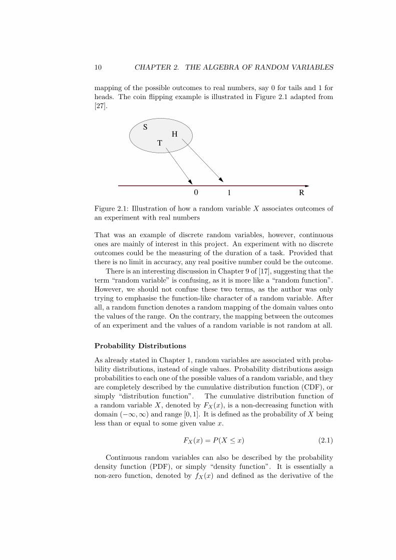
mapping of the possible outcomes to real numbers, say 0 for tails and 1 forheads. The coin flipping example is illustrated in Figure 2.1 adapted from[27].
SH
T
R0 1
Figure 2.1: Illustration of how a random variable X associates outcomes ofan experiment with real numbers
That was an example of discrete random variables, however, continuousones are mainly of interest in this project. An experiment with no discreteoutcomes could be the measuring of the duration of a task. Provided thatthere is no limit in accuracy, any real positive number could be the outcome.
There is an interesting discussion in Chapter 9 of [17], suggesting that theterm “random variable” is confusing, as it is more like a “random function”.However, we should not confuse these two terms, as the author was onlytrying to emphasise the function-like character of a random variable. Afterall, a random function denotes a random mapping of the domain values ontothe values of the range. On the contrary, the mapping between the outcomesof an experiment and the values of a random variable is not random at all.
Probability Distributions
As already stated in Chapter 1, random variables are associated with proba-bility distributions, instead of single values. Probability distributions assignprobabilities to each one of the possible values of a random variable, and theyare completely described by the cumulative distribution function (CDF), orsimply “distribution function”. The cumulative distribution function ofa random variable X, denoted by FX(x), is a non-decreasing function withdomain (−∞,∞) and range [0, 1]. It is defined as the probability of X beingless than or equal to some given value x.
FX(x) = P (X ≤ x) (2.1)
Continuous random variables can also be described by the probabilitydensity function (PDF), or simply “density function”. It is essentially anon-zero function, denoted by fX(x) and defined as the derivative of the

2.2. FUNCTIONS OF ONE RANDOM VARIABLE 11
distribution function.fX(x) =
dFX(x)dx
(2.2)
An interesting property of continuous distributions is that any event on itsown has probability equal to zero, despite the value of the density function.The density function at a point x should be interpreted as the probabilitythat the outcome lies in the nearby area. More formally, the probability ofan outcome lying within the interval [a, b] will be:
P (a ≤ X ≤ b) =∫ b
afX(x)dx (2.3)
On the other hand, each event of a discrete random variable is assignedwith a specific probability. If a probability of an event is zero, then it isjust impossible to happen. The probability mass function fX(x) is definedas the mapping of values x of a random variable X onto probabilities.
fX(x) = P (X = x) (2.4)
Eventually, it is also possible a random variable is both discrete andcontinuous. This means that its probability distribution possesses propertiesof a continuous distribution for certain areas of its domain, while for otherspossesses properties of a discrete one. The way such mixed distributions arehandled in terms of the project is described in Section 2.2.3.
2.2 Functions of One Random Variable
In the general case, a function g(X) of a random variable X is a compositefunction
Y = g(X) = g[X(ζ)] (2.5)
that has as domain the sample space S, since ζ are events of S. It is evidentthat the function g(X) maps events of S onto real values, which is consistentwith the definition of random variables given in Section 2.1. Thus, the resultY of g(X) is a random variable as well.
Examples of functions of one random variable are expressions such asX + 5 or min(X, 2). We will focus on the ones that are related to the fourbasic arithmetic operations, plus the minimum and the maximum.
2.2.1 Linear Functions
Most of the cases we are concerned with fall in the case of linear functions.More specifically, the cases that involve addition, subtraction, multiplicationand division of a random variable by a scalar value, are covered in thissection. A linear function g(X) of a random variable X is of the form:
Y = aX + b (2.6)

12 CHAPTER 2. THE ALGEBRA OF RANDOM VARIABLES
where a and b are scalar values. In Chapter 5 of [41], it is shown that thedistribution function of random variable Y can be expressed in terms of thedistribution function of X:
FY (y) = P
(X ≤ y − b
a
)= FX
(y − b
a
), a > 0 (2.7)
FY (y) = P
(X ≥ y − b
a
)= 1− FX
(y − b
a
), a < 0 (2.8)
We are also attaching the density fY (y) of the linear function of the randomvariable X. The proof can be found in [41] as well.
fY (y) =1|a|
fX
(y − b
a
)(2.9)
The Uniform Case We can see that a linear transformation, such as theone above, does not alter the form of the distribution function. Parameterb shifts the distribution function, while coefficient a scales it along the hori-zontal axis. For example, if X follows a uniform distribution, its distributionfunction will be of the form:
FX(x) =
0, x < c1
x−c1c2−c1
, c1 ≤ x < c2
1, c2 ≤ x
(2.10)
where c1, c2 are the endpoints of the distribution. In case a is positive,according to Equation (2.7) the second case of (2.10) becomes y−b−ac1
ac2−ac1. Since
the distribution function of X was right continuous, so must be its lineartransformation as well. Thus, the following equations should hold:
FY (c′1) = 0⇒ c′1 − b− ac1
ac2 − ac1= 0 (2.11)
limx→c′2
−FY = 1⇒ c′2 − b− ac1
ac2 − ac1= 1 (2.12)
By solving (2.11) and (2.12) we can find that Y follows a uniform distributionwith endpoints c′1 = ac1 + b and c′2 = ac2 + b. We can also use Equation(2.8) in a similar way to obtain the endpoints, c′1 = ac2 + b and c′2 = ac1 + bof the uniform variable Y for negative values of a. Summarising, a linearfunction of a uniform random variable X will be:
FY (y) =
0, y < ac1 + by−ac1+bac2−ac1
, ac1 + b ≤ y < ac2 + b, a > 01, y ≥ ac2 + b
(2.13)
FY (y) =
0, y < ac2 + by−ac2+bac1−ac2
, ac2 + b ≤ y < ac1 + b, a < 01, y ≥ ac1 + b
(2.14)

2.2. FUNCTIONS OF ONE RANDOM VARIABLE 13
The Gaussian Case The distribution function of a random variable Xfollowing a Gaussian distribution with mean µX and variance σ2
X will be:
FX(x) =12
+12erf
x− µX√2σ2
X
(2.15)
where erf(x) is the error function, which according to [1] is defined as:
erf(x) =2√π
∫ x
0e−t2dt (2.16)
By using Equation (2.7) again, considering positive a, we obtain:
FY (y) =12
+12erf
y − aµX − b√2a2σ2
X
, a > 0 (2.17)
So, we can see that Y is a Gaussian variable with mean µY = aµX + b andvariance σ2
Y = a2σ2X . Now for the negative values of a, if we use (2.8) we
obtain:
FY (y) =12− 1
2erf
y − aµX − b√2a2σ2
X
, a < 0 (2.18)
As reported in [1], error function is an odd function, which entails that−erf(x) = erf(−x). Thus, (2.18) will become:
FY (y) =12
+12erf
−y + aµX + b√2a2σ2
X
, a < 0 (2.19)
Eventually, (2.19) implies that the distribution of the result will be a Gaus-sian with mean µY = aµX + b and variance σ2
Y = a2σ2X , for a < 0 as well.
We can see that result for both uniform and Gaussian distributions aretractable and very easy to be estimated. Such findings seem to justify thechoice of the author to use this kind of distributions as components, in orderto describe more complex ones. So, we can apply any linear function to eachone of the components independently. The final result does not need to bere-approximated, as only the parameters of the mixture distributions willchange, not their form.
2.2.2 Division by Random Variables
Given that we already know the results of linear functions of random vari-ables, dividing by a random variable simply demands estimating the expres-sion 1/X, which does not fall in the linear case. In spite of this, it is still

14 CHAPTER 2. THE ALGEBRA OF RANDOM VARIABLES
within the range of operators we wish to implement in terms of the project.Again in Chapter 5 of [41], there is a proof that the probability densityfunction fY (y) of the random variable Y = 1/X will be:
fY (y) =1y2
fX
(1y
)(2.20)
One way to obtain the distribution function would be to compute the indef-inite integral of (2.20). Indeed, by applying the chain rule we can find thatthe distribution function will be of the form −FX( 1
y ) + c. We can not findthe constant c for any kind of distribution though, as we do not know itssupport. Instead, we can think of the definition of the distribution functionFY (y), which is P (Y ≤ y) or P (1/X ≤ y). So we can discriminate thefollowing cases:
• If y > 0, then we have 1/x ≤ y
– for x ≥ 1/y, if x > 0
– always, if x < 0
Hence:
FY (y) = P (X ≥ 1/y) + P (X ≤ 0) = 1− FX
(1y
)+ FX(0) (2.21)
• If y < 0, then we have 1/x ≤ y
– never, if x > 0
– for x ≥ 1/y, if x < 0
Hence:
FY (y) = P (X ≥ 1/y)− P (X ≥ 0) = −FX
(1y
)+ FX(0) (2.22)
The equations above make clear that the density and the distribution func-tions of the division by a random variable can be expressed in terms ofthe original density and distribution functions repsectively. These functionshowever, are known for any kind of distribution in terms of the project,since the distributions are supposed to be approximated by mixture models.So, it is possible to estimate the quotient 1/X for any distribution of Xby applying Equations (2.20), (2.21) and (2.22) directly, instead of on eachone of the components individually. Eventually, we can re-approximate thisintermediate result with a new mixture model.
Together with the linear functions in the previous section, we have cov-ered all the cases of the four basic arithmetic operations between randomand scalar variables.

2.3. SUM AND DIFFERENCE OF RANDOM VARIABLES 15
2.2.3 Minimum and Maximum between a Random Variableand a Constant
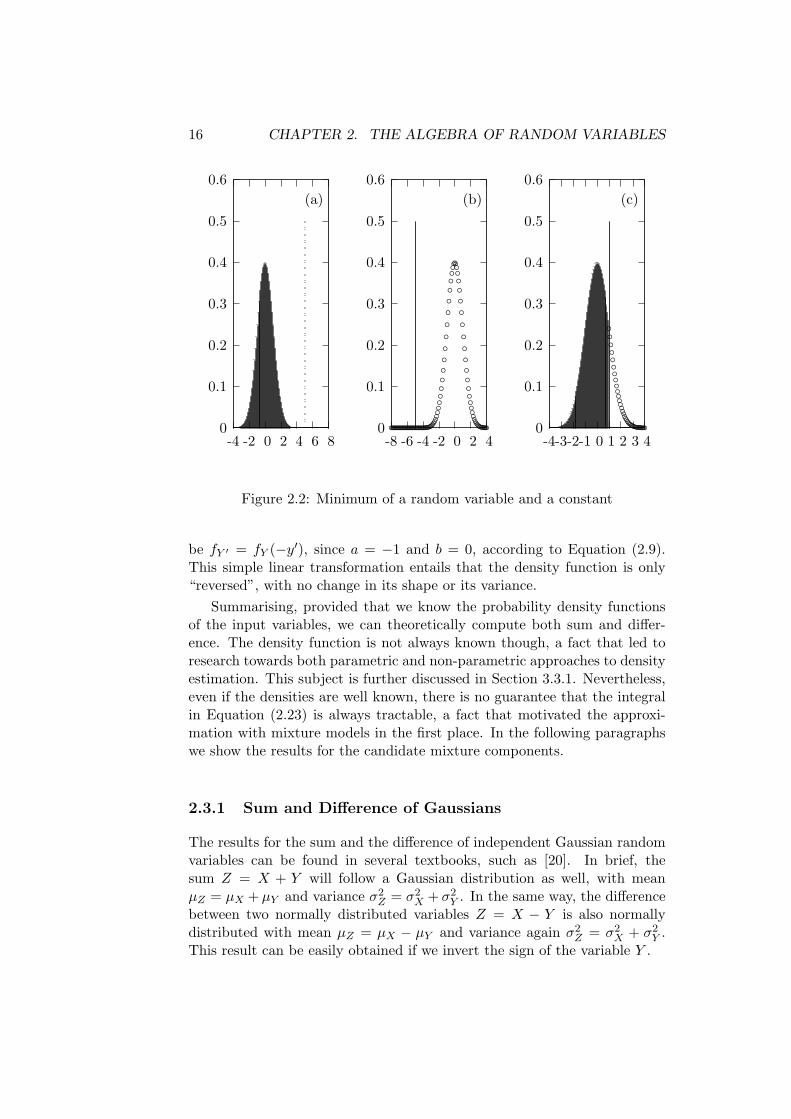
The list of functions to be implemented also includes the minimum and themaximum of random variables, as we have seen in the introduction. In thissection, we will have a look on the expressions min(X, a) and max(X, a),where X is a random variable and a is a scalar value. Starting form theminimum, we can distinguish three cases, also illustrated in Figure 2.2:
• If the value a lies after the whole support of the distribution of X,then the result of min(X, a) will be the random variable X itself.
• If the value a lies before the whole support of the distribution of X,then the result of min(X, a) will always be the scalar value a. In termsof continuous probability distributions, this result can be thought ofas a Gaussian distribution with mean a and zero variance (or reallyclose to zero). In the current project, such results are approximatedwith low variance Gaussian spikes.
• If the value a lies within the support of the distribution of X, theresult will be a mixed random variable. More specifically, the contin-uous part of the result will be in the range (−∞, a), and the densityfunction in that range will be the same as that of X, while its areawill be integrated up to F (a). The remaining 1 − F (a) area is actu-ally “vaporised” to the probability of the value a. As we did in theprevious case, the probability of a will be expressed as an extremelytight Gaussian. So, the final result will essentially be a mixture modelconsisting of these two components.
It is straightforward to produce similar results for the maximum, just bytaking into account the complementary areas of the support of X.
2.3 Sum and Difference of Random Variables
The density function of the sum of two independent random variables X andY , is the convolution of the density functions of the operant distributions[47], fXx and fY (y) respectively. The random variable Z = X +Y will havedensity function:
(fX ∗ fY )(z) =∫ ∞
−∞fX(z − y)fY (y)dy =
∫ ∞
−∞fY (z − x)fX(x)dx (2.23)
The difference of two random variables Z = X − Y can be regardedas the sum Z = X + Y ′, whose second argument is Y ′ = −Y . The useof a negative sign on a random variable falls in the linear function caseexplained in Section 2.2.1. More specifically, the density function of Y will
16 CHAPTER 2. THE ALGEBRA OF RANDOM VARIABLES
0
0.1
0.2
0.3
0.4
0.5
0.6
-4 -2 0 2 4 6 8
(a)
0
0.1
0.2
0.3
0.4
0.5
0.6
-8 -6 -4 -2 0 2 4
(b)
bbbbbbbbbbbbbbbbbbbbbbbbbbbbbbbbbbbbbbbbbbbbbbbbbbbbbbbbbbbbbbbbbbbbbbbbbbbbbbbbbbbbbbbbbbbbbbbbbbbb 0
0.1
0.2
0.3
0.4
0.5
0.6
-4-3-2-1 0 1 2 3 4
(c)
bbbbbbbbbbbbbbbbbbbbbbbbbbbbbbbbbbbbbb
Figure 2.2: Minimum of a random variable and a constant
be fY ′ = fY (−y′), since a = −1 and b = 0, according to Equation (2.9).This simple linear transformation entails that the density function is only“reversed”, with no change in its shape or its variance.
Summarising, provided that we know the probability density functionsof the input variables, we can theoretically compute both sum and differ-ence. The density function is not always known though, a fact that led toresearch towards both parametric and non-parametric approaches to densityestimation. This subject is further discussed in Section 3.3.1. Nevertheless,even if the densities are well known, there is no guarantee that the integralin Equation (2.23) is always tractable, a fact that motivated the approxi-mation with mixture models in the first place. In the following paragraphswe show the results for the candidate mixture components.
2.3.1 Sum and Difference of Gaussians
The results for the sum and the difference of independent Gaussian randomvariables can be found in several textbooks, such as [20]. In brief, thesum Z = X + Y will follow a Gaussian distribution as well, with meanµZ = µX + µY and variance σ2
Z = σ2X + σ2
Y . In the same way, the differencebetween two normally distributed variables Z = X − Y is also normallydistributed with mean µZ = µX − µY and variance again σ2
Z = σ2X + σ2
Y .This result can be easily obtained if we invert the sign of the variable Y .

2.3. SUM AND DIFFERENCE OF RANDOM VARIABLES 17
2.3.2 Sum and Difference of Uniforms
Although both convolution and cross-correlation of uniform densities arerelatively easy to be computed, as we will see the results do not fall intothe known types of densities, in contrast with the Gaussian example. Theauthors of [8] provide a form for the convolution of N independent uniformlydistributes random variables. Since we are interested in binary operationsonly, we present the formula for the sum of two random variables that followuniform distributions U(a1, b1) and U(a2, b2).
• If a1 + b2 < a2 + b1
fZ(z) =
0, z < a1 + a2z−(a1+a2)
(b1−a1)(b2−a2) , a1 + a2 ≤ z < a1 + b2
1b1−a1
, a1 + b2 ≤ z < a2 + b1−z+(b1+b2)
(b1−a1)(b2−a2) , a2 + b1 ≤ z < b1 + b2
0, b1 + b2 ≤ z
(2.24)
FZ(z) =
0, z < a1 + a2z2−2z(a1+a2)
2(b1−a1)(b2−a2) + c1, a1 + a2 ≤ z < a1 + b2
zb1−a1
+ c2, a1 + b2 ≤ z < a2 + b1−z2+2z(b1+b2)2(b1−a1)(b2−a2) + c3, a2 + b1 ≤ z < b1 + b2
1, b1 + b2 ≤ z
(2.25)
• If a1 + b2 > a2 + b1
fZ(z) =
0, z < a1 + a2z−(a1+a2)
(b1−a1)(b2−a2) , a1 + a2 ≤ z < a2 + b1
1b2−a2
, a2 + b1 ≤ z < a1 + b2−z+(b1+b2)
(b1−a1)(b2−a2) , a1 + b2 ≤ z < b1 + b2
0, b1 + b2 ≤ z
(2.26)
FZ(z) =
0, z < a1 + a2z2−2z(a1+a2)
2(b1−a1)(b2−a2) + c1, a1 + a2 ≤ z < a2 + b1
1b2−a2
+ c2, a2 + b1 ≤ z < a1 + b2−z2+2z(b1+b2)2(b1−a1)(b2−a2) + c3, a1 + b2 ≤ z < b1 + b2
1, b1 + b2 ≤ z
(2.27)
18 CHAPTER 2. THE ALGEBRA OF RANDOM VARIABLES
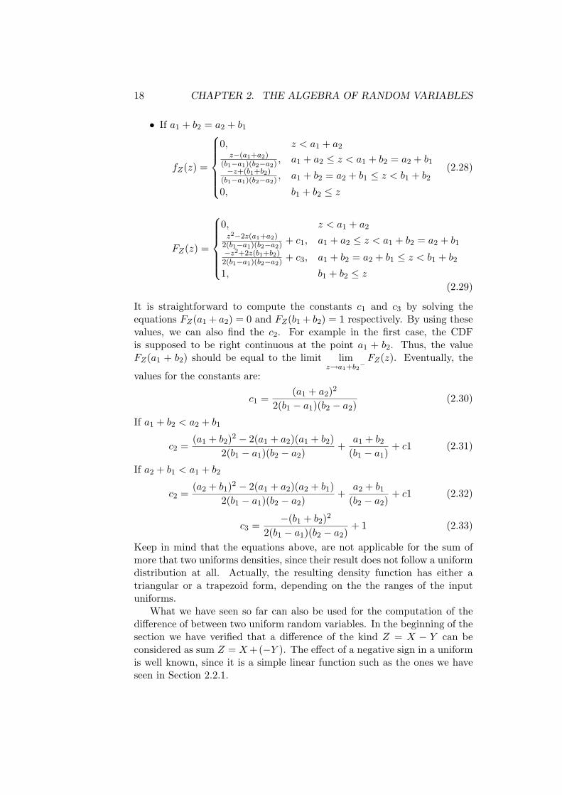
• If a1 + b2 = a2 + b1
fZ(z) =
0, z < a1 + a2
z−(a1+a2)(b1−a1)(b2−a2) , a1 + a2 ≤ z < a1 + b2 = a2 + b1
−z+(b1+b2)(b1−a1)(b2−a2) , a1 + b2 = a2 + b1 ≤ z < b1 + b2
0, b1 + b2 ≤ z
(2.28)
FZ(z) =
0, z < a1 + a2
z2−2z(a1+a2)2(b1−a1)(b2−a2) + c1, a1 + a2 ≤ z < a1 + b2 = a2 + b1
−z2+2z(b1+b2)2(b1−a1)(b2−a2) + c3, a1 + b2 = a2 + b1 ≤ z < b1 + b2
1, b1 + b2 ≤ z
(2.29)
It is straightforward to compute the constants c1 and c3 by solving theequations FZ(a1 + a2) = 0 and FZ(b1 + b2) = 1 respectively. By using thesevalues, we can also find the c2. For example in the first case, the CDFis supposed to be right continuous at the point a1 + b2. Thus, the valueFZ(a1 + b2) should be equal to the limit lim
z→a1+b2−
FZ(z). Eventually, the
values for the constants are:
c1 =(a1 + a2)2
2(b1 − a1)(b2 − a2)(2.30)
If a1 + b2 < a2 + b1
c2 =(a1 + b2)2 − 2(a1 + a2)(a1 + b2)
2(b1 − a1)(b2 − a2)+
a1 + b2
(b1 − a1)+ c1 (2.31)
If a2 + b1 < a1 + b2
c2 =(a2 + b1)2 − 2(a1 + a2)(a2 + b1)
2(b1 − a1)(b2 − a2)+
a2 + b1
(b2 − a2)+ c1 (2.32)
c3 =−(b1 + b2)2
2(b1 − a1)(b2 − a2)+ 1 (2.33)
Keep in mind that the equations above, are not applicable for the sum ofmore that two uniforms densities, since their result does not follow a uniformdistribution at all. Actually, the resulting density function has either atriangular or a trapezoid form, depending on the the ranges of the inputuniforms.
What we have seen so far can also be used for the computation of thedifference of between two uniform random variables. In the beginning of thesection we have verified that a difference of the kind Z = X − Y can beconsidered as sum Z = X +(−Y ). The effect of a negative sign in a uniformis well known, since it is a simple linear function such as the ones we haveseen in Section 2.2.1.
2.4. PRODUCT AND RATIO OF RANDOM VARIABLES 19
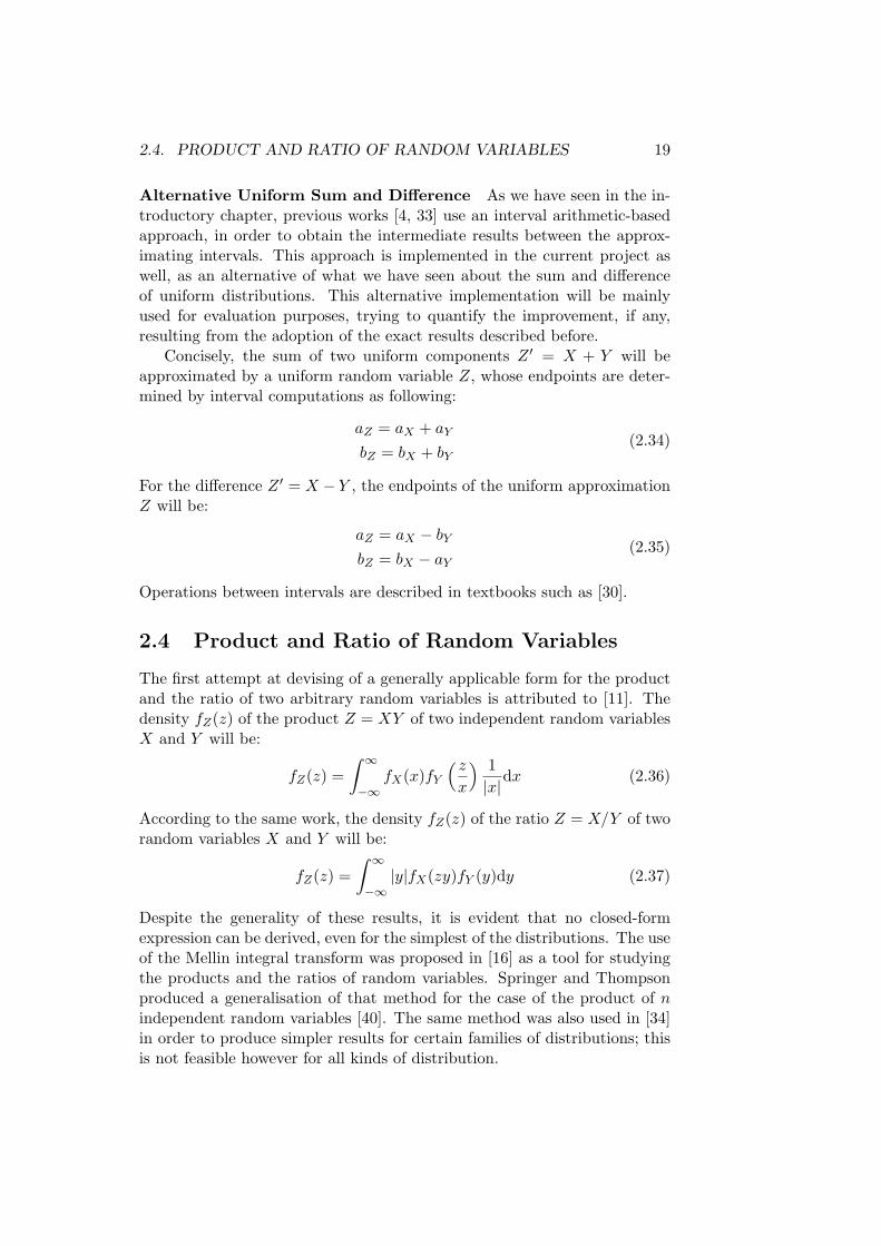
Alternative Uniform Sum and Difference As we have seen in the in-troductory chapter, previous works [4, 33] use an interval arithmetic-basedapproach, in order to obtain the intermediate results between the approx-imating intervals. This approach is implemented in the current project aswell, as an alternative of what we have seen about the sum and differenceof uniform distributions. This alternative implementation will be mainlyused for evaluation purposes, trying to quantify the improvement, if any,resulting from the adoption of the exact results described before.
Concisely, the sum of two uniform components Z ′ = X + Y will beapproximated by a uniform random variable Z, whose endpoints are deter-mined by interval computations as following:
aZ = aX + aY
bZ = bX + bY(2.34)
For the difference Z ′ = X − Y , the endpoints of the uniform approximationZ will be:
aZ = aX − bY
bZ = bX − aY(2.35)
Operations between intervals are described in textbooks such as [30].
2.4 Product and Ratio of Random Variables
The first attempt at devising of a generally applicable form for the productand the ratio of two arbitrary random variables is attributed to [11]. Thedensity fZ(z) of the product Z = XY of two independent random variablesX and Y will be:
fZ(z) =∫ ∞
−∞fX(x)fY
( z
x
) 1|x|
dx (2.36)
According to the same work, the density fZ(z) of the ratio Z = X/Y of tworandom variables X and Y will be:
fZ(z) =∫ ∞
−∞|y|fX(zy)fY (y)dy (2.37)
Despite the generality of these results, it is evident that no closed-formexpression can be derived, even for the simplest of the distributions. The useof the Mellin integral transform was proposed in [16] as a tool for studyingthe products and the ratios of random variables. Springer and Thompsonproduced a generalisation of that method for the case of the product of nindependent random variables [40]. The same method was also used in [34]in order to produce simpler results for certain families of distributions; thisis not feasible however for all kinds of distribution.

20 CHAPTER 2. THE ALGEBRA OF RANDOM VARIABLES
2.4.1 Approximation for the Product of Gaussians
A form for the product of two arbitrary independent normally distributedvariables is given in [10], however it is not considered as a closed-form ex-pression, since it involves integrals. The difficulties in the computation ofintegrals gave rise to approximate methods. The normality of the productof two normally distributed variables was first investigated in [3], and laterexperimentally verified in [23] for a number of cases. More specifically, itwas proven that the product of two Gaussian X and Y variables approachesa normal curve when:
ρX =µX
σX→∞, ρY =
µY
σY→∞ (2.38)
In this case, the mean and the variance of the Gaussian variable Z thatapproximates the product Z ′ = XY will be:
µZ = µXµY (2.39)
σ2Z = σ2
Xσ2Y + µ2
Y σ2X + µ2
Xσ2Y (2.40)
Equations (2.39) and (2.40) were adapted from [23], with zero correlationcoefficient though, as we are interested in independent variables only.
So, it seems acceptable to approximate products of Gaussian compo-nents, instead of using exact analytic solutions. The preconditions underwhich this approximation is valid are summarised in (2.38), and they willalmost always be true if the variances of the input distributions are close tozero. In fact, that is the case for our Gaussian approximation components,since the idea is to approximate the original density with a large number oflow variance overlapping Gaussian mixture components.
2.4.2 Approximation for the Ratio of Gaussians
A general form for the ratio of two correlated Gaussian variables was firstintroduced by D.V. Hinkley in [25]. The formula invented by Hinkley in-cludes a correlation variable ρ, which captures the dependency between theinput variables. We present this formula based on zero correlation though,as we are mainly interested in the ratio of independent X and Y . Thus, thedensity function of the ratio Z = X/Y will be:
fZ(z) =b(z)c(z)a3(z)
1√2πσXσY
[2Φ
(b(z)a(z)
)− 1
]+
1a2(z)πσXσY
e−1/2
„µ2
Xσ2
X
+µ2
Xσ2
X
«
(2.41)
2.4. PRODUCT AND RATIO OF RANDOM VARIABLES 21
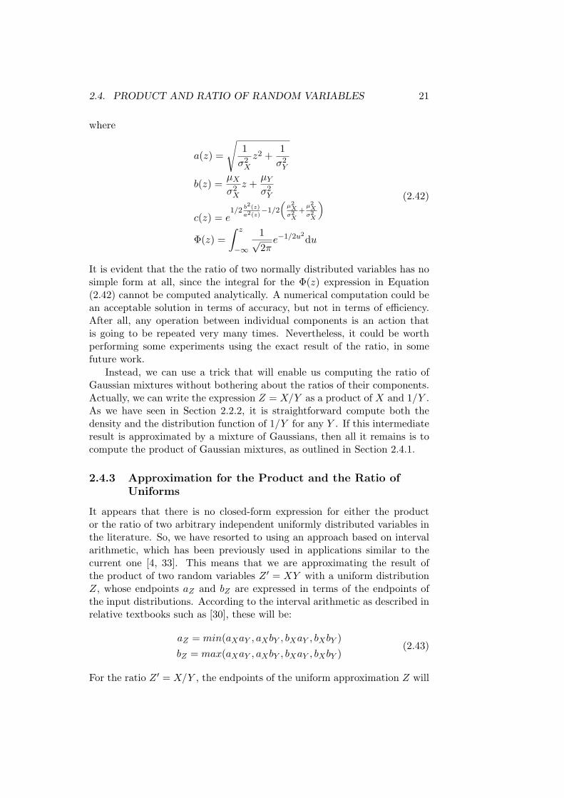
where
a(z) =
√1
σ2X
z2 +1
σ2Y
b(z) =µX
σ2X
z +µY
σ2Y
c(z) = e1/2
b2(z)
a2(z)−1/2
„µ2
Xσ2
X
+µ2
Xσ2
X
«
Φ(z) =∫ z
−∞
1√2π
e−1/2u2du
(2.42)
It is evident that the the ratio of two normally distributed variables has nosimple form at all, since the integral for the Φ(z) expression in Equation(2.42) cannot be computed analytically. A numerical computation could bean acceptable solution in terms of accuracy, but not in terms of efficiency.After all, any operation between individual components is an action thatis going to be repeated very many times. Nevertheless, it could be worthperforming some experiments using the exact result of the ratio, in somefuture work.
Instead, we can use a trick that will enable us computing the ratio ofGaussian mixtures without bothering about the ratios of their components.Actually, we can write the expression Z = X/Y as a product of X and 1/Y .As we have seen in Section 2.2.2, it is straightforward compute both thedensity and the distribution function of 1/Y for any Y . If this intermediateresult is approximated by a mixture of Gaussians, then all it remains is tocompute the product of Gaussian mixtures, as outlined in Section 2.4.1.
2.4.3 Approximation for the Product and the Ratio ofUniforms
It appears that there is no closed-form expression for either the productor the ratio of two arbitrary independent uniformly distributed variables inthe literature. So, we have resorted to using an approach based on intervalarithmetic, which has been previously used in applications similar to thecurrent one [4, 33]. This means that we are approximating the result ofthe product of two random variables Z ′ = XY with a uniform distributionZ, whose endpoints aZ and bZ are expressed in terms of the endpoints ofthe input distributions. According to the interval arithmetic as described inrelative textbooks such as [30], these will be:
aZ = min(aXaY , aXbY , bXaY , bXbY )bZ = max(aXaY , aXbY , bXaY , bXbY )
(2.43)
For the ratio Z ′ = X/Y , the endpoints of the uniform approximation Z will

22 CHAPTER 2. THE ALGEBRA OF RANDOM VARIABLES
be:
aZ = min(aX/aY , aX/bY , bX/aY , bX/bY )bZ = max(aX/aY , aX/bY , bX/aY , bX/bY )
(2.44)
Experimentation with a better approximation of the actual results could besubject of future work.
2.5 Minimum and Maximum of Random Variables
Proofs for the results of the minimum and the maximum between two in-dependent random variables can be found in several textbooks [41, 46].The probability density function and the cumulative distribution functionof Z = min(X, Y ) for X and Y independent will be:
fZ(z) = fX(z)(1− FY (z)) + fY (z)(1− FX(z)) (2.45)
FZ(z) = FX(z) + FY (z)− FX(z)FY (z) (2.46)
The probability density function and the cumulative distribution functionof Z = max(X, Y ) for X and Y independent will be:
fZ(z) = fX(z)FY (z) + fY (z)FX(z) (2.47)
FZ(z) = FX(z)FY (z) (2.48)
It is evident that the minimum and the maximum of two random vari-ables is written as a closed-form expression of the density and the distribu-tion functions of the inputs. Actually, these findings are more than conve-nient, as these functions are always known in this project. More precisely,all the distributions are going to be approximated by mixture models withwell known forms for their density and distribution functions. Thus, thereis no need to perform these operations between the mixture componentsindividually. Instead, we can store either the minimum or the maximumin an intermediate result, whose density and distribution functions can befound using either (2.45) and (2.45), or (2.47) and (2.47). Eventually, wecan re-approximate this intermediate result with a mixture model, so as tobe used in future computations. This direct approach saves us from theO(N2) complexity of performing operations on components.
Chapter 3
The Stochastic Library
The Stochastic library is the result of the current research. As its nameimplies, it provides a framework for manipulating stochastic variables. Thelibrary is written in standard C++, in order to ensure the portability ofthe source code. C was probably the most obvious option for maximisingefficiency, however, C++ was preferred so as to incorporate the Object-Oriented principles into the project. So, the choice of the programminglanguage is an attempt to combine efficiency, modularity and portability.
The main idea is that the user will have access to a new data type thatrepresents continuous random variables. The user should be able to createinstances of the random variable data type and define the probability dis-tribution that these instances follow. The framework should also allow theuser to ask questions about the probability and cumulative probability ofspecific values, and produce samples from the distributions defined. Finally,the random variable type should be used in arithmetic operations so that theresults are consistent with the theoretical ones presented in Chapter 2. Byconsistent, we mean that the resulting random variables have distributionsthat are good approximations to the real ones. The quality of this approxi-mation will be evaluated in Chapter 4. All this functionality is implementedin the RandomVariable class.
Apart from the RandomVariable class, the user will have access to anumber of “concrete” distribution classes, which represent various proba-bility distributions of the real world. We emphasise “concrete” since all ofthem are subclasses of abstract data types, as we will see on the next sec-tion. The full list of the concrete distributions can be found in Appendix A.Eventually, random variables can be initialised by either using known distri-butions or fitting distributions to real data. The following code illustratesa simple example of creating RandomVariable instances and using them inoperations.
23

24 CHAPTER 3. THE STOCHASTIC LIBRARY
#include <stochastic.h>
using namespace stochastic;
int main(){
RandomVariable a = new Gaussian (0,1);RandomVariable b = new EmpiricalDistribution ("data ");RandomVariable c;c = a + b;return c.getDistribution (). nextSample ();
}
RandomVariable a follows a standard normal distribution, while instanceb has the distribution of the data contained in the file data. So, the resultof the sum of these variables is stored in RandomVariable c. Finally, theprogram returns a sample from the sum distribution that is stored in c. Inthe sections that follow, we will see more details of the implementation.
3.1 Class Structure
As we have seen so far, the main functionality involves assigning distribu-tions to random variables before performing useful tasks with them. In thissection, we will see how the RandomVariable class is associated with the var-ious distributions and the other modules of the system. These associationsare visible in the class diagram depicted in Figure 3.1.
RandomVariable Distribution
PiecewiseBase
Figure 3.1: Class diagram of Stochastic library
The RandomVariable class includes methods and overloaded operatorsthat correspond to functions of random variables. The way that distributionsare assigned to random variables is captured by an one-to-one associationwith the Distribution class. No instances of Distribution can be created sinceit is abstract — however, it is the base of all the “concrete” distributions.

3.1. CLASS STRUCTURE 25
In other words, it features a number of pure virtual methods that definethe interface for any kind of probability distribution. Furthermore, theRandomVariable class is also associated with the PiecewiseBase class, whichis an abstraction of the approximating distributions.
Inheritance Hierarchy for Distribution classes All classes derivedfrom the abstract Distribution are forced to comply with the specified inter-face. However, concrete probability distributions are further distinguishedinto groups. This distinction is defined by the inheritance hierarchy ofclasses, as depicted in Figure 3.2.
Distribution
MixtureComponentEmpiricalDistribution
Exponential
Cauchy
Gaussian
MixtureModel
PiecewiseBase
PiecewiseGaussian
PiecewiseUniformUniform
Figure 3.2: The inheritance diagram for Distribution classes
One of the principal goals of the architecture design was to support awide range of probability distributions. The classes that directly derivedfrom the Distribution represent the three main types of input distributions:
• Distributions with known density functionsSuch distributions can also be components of a mixture model, so theyimplement the abstract MixtureComponent class.
• Mixture modelsIn this case, the probability density function is expressed as a combi-nation of the probability densities of mixture components.
• Distributions of real dataThe EmpiricalDistribution class approximates the distribution of a
26 CHAPTER 3. THE STOCHASTIC LIBRARY
given dataset using a non-parametric approach. A more detailed dis-cussion can be found in Section 3.3.1.
One could argue that any kind of distribution could be used as a mixturecomponent, instead of only the ones with known density functions. However,only the latter are considered eligible by the author, so as to ensure thatmixtures will have tractable forms as well. The knowledge of density func-tions is essential in order to perform useful operations on random variables.Thus, mixture models are used to estimate the density of non-tractable dis-tributions. For example, an EmpiricalDistribution object could capture theexact distribution of a dataset, in some non-parametric form. Even so, sucha distribution can be approximated by a mixture model, as discussed inSection 3.4.
The class that represents the special family of mixture models used forapproximating other distributions is the abstract PiecewiseBase. It is notedthat these approximations will also be used to perform arithmetic operationson random variables, which is among the primary goals of this research. Inbrief, whilst mixture models are allowed to have any number of componentsthat can even be of different type, the classes derived from the PiecewiseBaseare more restricted. Actually, the number and the type of componentsaffect the approximation procedure, which has an effect on both accuracyand efficiency. So, the choice of these two parameters should be the users’.Approximation with either mixtures of uniforms or mixtures of Gaussian isavailable. A set of pure virtual methods in the base class imply that theimplementations should be able to approximate any input distribution, interms of the project, and carry out operations between single components.In fact, the implementation of the specific module was a major issue of thisresearch, hence design options are discussed in detail in sections 3.4.1 and3.4.2.
3.2 Common Distribution Operations
As we have seen, the Distribution class is an abstraction for all the kinds ofdistributions featured in the current project. What really distinguishes onedistribution from another are its probability density function and its cumu-lative distribution function1. So, the derived classes are forced to implementthe pure virtual methods that correspond to these functions.
Since these two functions are supposed to be known for any distribution(in some cases they are approximated, as we see in Section 3.3), we can usethem to perform operations implemented in common for all the distributions.
1Actually, only one of them is needed to define a probability distribution, but both areused for convenience
3.2. COMMON DISTRIBUTION OPERATIONS 27
3.2.1 Sampling
Most of the sampling methods demand that we sample from a uniform dis-tribution over the interval (0, 1). Actually, standard C++ does provide afunction that generates pseudo-random integers uniformly distributed over[0, RAND MAX], which can be easily modified to fit our needs, by simply di-viding by RAND MAX+ 1. The pseudo-random property is actually desirable,since any experiment can be repeatable in this way.
It is noted that many authors [6, 35] prefer Markov Chain Monte Carlomethods, especially in the case of multi-dimensional variables. Neverthe-less, since we only have one-dimensional continuous random variables, thefollowing methods are both efficient and convenient.
Inverse Transform Sampling
Inverse transform sampling is based upon Theorem 1, adapted from [15],where also a proof of which can be found.
Theorem 1 If F is a continuous cumulative distribution function on < andF−1 is its inverse function defined by:
F−1(u) = inf{x|F (x) = u, 0 < u < 1}
Then F−1(u) has distribution F , where u is a uniform random variable on[0, 1].
Thus, once the inverse of the cumulative function of a random variable isexplictly known, we can sample from it by using an algorithm summarisedin the following steps:
1. Draw a sample u from U(0, 1)
2. Compute and return F−1(u)
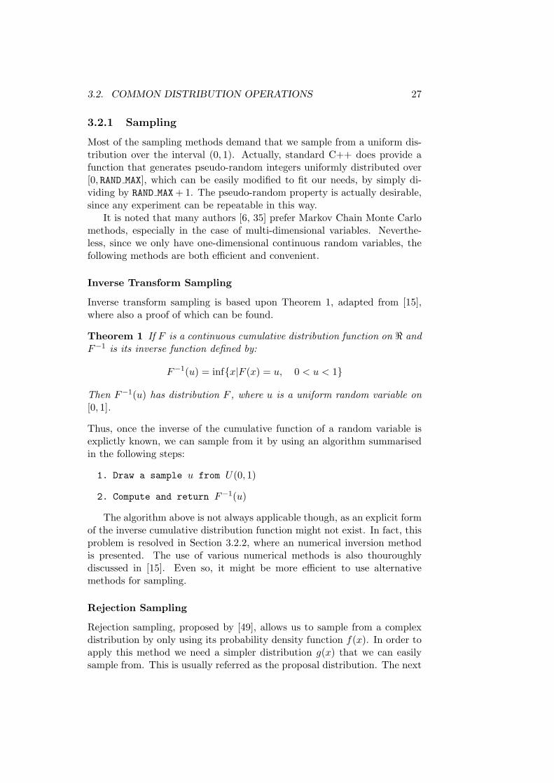
The algorithm above is not always applicable though, as an explicit formof the inverse cumulative distribution function might not exist. In fact, thisproblem is resolved in Section 3.2.2, where an numerical inversion methodis presented. The use of various numerical methods is also thouroughlydiscussed in [15]. Even so, it might be more efficient to use alternativemethods for sampling.
Rejection Sampling
Rejection sampling, proposed by [49], allows us to sample from a complexdistribution by only using its probability density function f(x). In order toapply this method we need a simpler distribution g(x) that we can easilysample from. This is usually referred as the proposal distribution. The next
28 CHAPTER 3. THE STOCHASTIC LIBRARY
step is to find a constant k such that kg(x) ≥ f(x) for all values of x. In brief,we sample from the proposal distribution and we occasionally reject samplesso that the remaining ones are consistent with the original distribution. Aformal definition of the algorithm is summarised in the following steps:
1. Draw a sample x from the proposal distribution g(x)
2. Draw a sample u from U(0, 1)
3. Accept x, if u < f(x)kg(x)
4. Else go to step 1
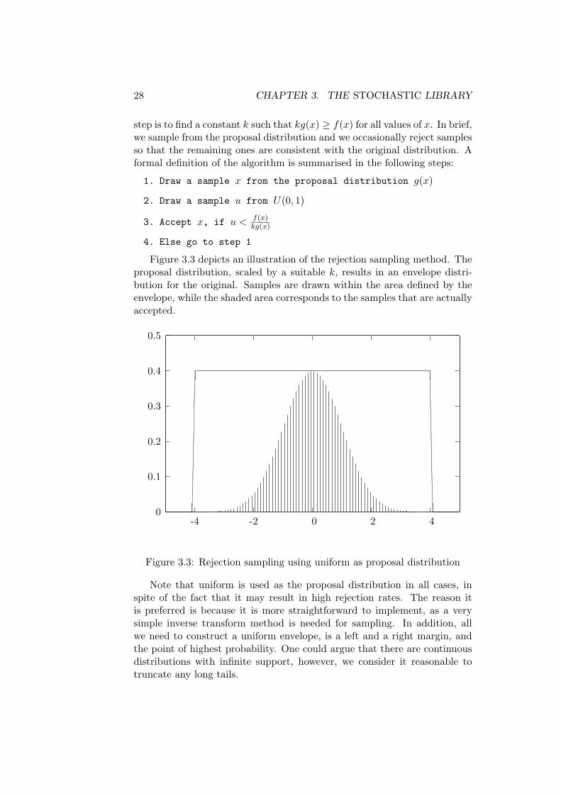
Figure 3.3 depicts an illustration of the rejection sampling method. Theproposal distribution, scaled by a suitable k, results in an envelope distri-bution for the original. Samples are drawn within the area defined by theenvelope, while the shaded area corresponds to the samples that are actuallyaccepted.
0
0.1
0.2
0.3
0.4
0.5
-4 -2 0 2 4
Figure 3.3: Rejection sampling using uniform as proposal distribution
Note that uniform is used as the proposal distribution in all cases, inspite of the fact that it may result in high rejection rates. The reason itis preferred is because it is more straightforward to implement, as a verysimple inverse transform method is needed for sampling. In addition, allwe need to construct a uniform envelope, is a left and a right margin, andthe point of highest probability. One could argue that there are continuousdistributions with infinite support, however, we consider it reasonable totruncate any long tails.

3.2. COMMON DISTRIBUTION OPERATIONS 29
3.2.2 The Quantile Function
In this section we discuss the numerical computation of the inverse cumula-tive distribution function, which is also known as “quantile function”, a termfirst introduced in [43]. Its importance has been already made clear tryingto sample from a distribution, in Section 3.2.1. Since explicit forms onlyexist for a limited number of distributions, a numerical method has beenadopted as a standard implementation in the abstract Distribution class.Some distributions, such as the Gaussian or the uniform, overload the orig-inal function, taking advantage of more efficient known quantile functions.The classes that make use of a formal definition of the quantile function,instead of the numerical solution, are noted in Appendix A.
The computation of the quantile function, which is denoted by Q(p) with0 ≤ p ≤ 1, can be thought of as the solution of the following equation withrespect to x, where F (x) is the cumulative distribution function:
F (x)− p = 0 (3.1)
A numerical solution involves the use of a root-finding algorithm, such asthe bisection method outlined below:
1. Let [a, b] interval that contains the solution
2. x← a+b2
3. if (F (a)− p) ∗ (F (x)− p) ≥ 0
a← x
4. else
b← x
5. if b− a ≥ 2δ
go to 2
6. else
return x
The use of any numerical algorithm implies that the true solution is approxi-mated. The quantity δ in the stopping criterion corresponds to the accuracyof the estimated solution.
According to [15], bisection exhibits slow convergence, in comparisonwith other algorithms such the secant method, or the Newton-Raphsonmethod. Nevertheless, in contrast with other methods, bisection is boundto converge if the initial interval [a, b] does contain the solution. In fact, itis pretty safe to assume that we can always find an initial interval [a, b] suchthat contains the solution, in the context of probability distributions. The

30 CHAPTER 3. THE STOCHASTIC LIBRARY
initial interval will be the one that contains the support of the distribution.In the case of distributions with infinite support, we can safely truncatethem so as to consider the 99.9% of the support.
3.3 Exceptional Distributions
The majority of the probability distributions implemented have simple para-metric forms. The parameters that govern each distribution are stored asprivate members in the classes that implement them. Therefore, there aremethods that make use of these parameters to carry out tasks such as com-puting the density and distribution functions. For example, the computationof probability density function involves applying the corresponding equationfor each distribution. The full list can be found in Appendix A. However,in this section, we will have a closer look at how sampling is performed anddensity and distribution functions are computed, for distributions with nosimple parametric form.
3.3.1 The Empirical Distribution
In order to make the system useful, it is essential that there is a way of ini-tialising the random variables using real data. The distribution of a datasetcan be expressed either in a specific functional form or not. The first case isknown as the parametric approach, as we assume that the data is drawn froma probability distribution that can be described by a finite set of parameters.For example, assuming that the underlying distribution for a given a datasetis a Gaussian, we can compute the mean and the variance that best explainthe data. The computation can be performed by using various methods,including “Maximum Likelihood” and “Bayesian Inference” [6]. Despitethe fact that Bayesian inference is the the method of preference of manyauthors [6, 35], the strong assumptions that it relies on, sometimes resultin poor approximation of a real distribution. For example, it is impossiblethat any single Gaussian approximates well a multimodal distribution.
On the contrary, non-parametric statistics make few assumptions aboutthe form of the underlying distribution. The distinction between the para-metric and the non-parametric case was first reported in [52]. Typical exam-ples of non-parametric density estimation are histograms and Parzen windowmethod [42], also known as kernel density estimation. One of the disad-vantages of the histograms is that they have discontinuities that may donot reflect the underlying distribution’s real nature. The kernel density es-timation is the approach chosen by the author, since it produces continuousdensity estimations, in contrast with histograms. However, a drawback ofthe method is the fact that it uses the whole dataset. Even so, it has beenconsidered as more important to represent the distribution of input data as

3.3. EXCEPTIONAL DISTRIBUTIONS 31
accurately as possible. After all, the user has always the choice of discardinga large dataset, by using an approximation — a mixture model, for example.
So, EmpiricalDistribution class is the one responsible for representingdistributions of input datasets, and is named after the empirical distributionfunction. The latter is the cumulative distribution function of the data,denoted by FN (x), where N is the total number of instances in the dataset.According to [28], it is equal to the proportion of sample values that are
less or equal to the value x.
FN (x) =number of samples ≤ x
N(3.2)
Equation (3.2) is actually used to estimate the cumulative distribution atany datapoint. In order to estimate the probability density function, wemake use of the Parzen window method. Given x1, x2, . . . , xN independentand identically distributed datapoints, the probability density function at apoint x is approximated by:
fh(x) =1
Nh
N∑i=1
K
(x− xi
h
)(3.3)
where kernel K was chosen to be the standard Gaussian for convenience.After all a continuous kernel is required to ensure that the estimated densitywill have no artificial discontinuities.
K
(x− xi
h
)=
1√2π
e−(x−xi)
2
2h2 (3.4)
Parameter h, which is called bandwidth, plays the role of a smoothing pa-rameter. As, shown in Figure 3.4, too large a bandwidth can result inmodels that are too smooth to capture multimodal distributions. On theother hand, too small a bandwidth can result in an over-sensitive modelwith a lot of structure that does not exist.
As reported in [50], the choice of banwidth is more crucial than the choiceof the kernel. In order to determine the bandwidth, we have adopted thefollowing rule, as defined in [18]:
h = 2Q(0.75)−Q(0.25)
3√
N(3.5)
where Q(x) is the quantile function. An example kernel density estimationusing (3.5) is illustrated in Figure 3.5.
3.3.2 Mixture Models
The term mixture model refers to random variables that have mixture den-sities. More specifically, the probability density function is expressed as

32 CHAPTER 3. THE STOCHASTIC LIBRARY
0
0.05
0.1
0.15
0.2
0.25
-6 -4 -2 0 2 4 6 8 10
h = 1
0
0.05
0.1
0.15
0.2
0.25
-6 -4 -2 0 2 4 6 8 10
h = 0.005
Figure 3.4: Kernel density estimation with standard Gaussian kernel usingvarying bandwidth h, where the dotted line is the true density
0
0.05
0.1
0.15
0.2
0.25
-6 -4 -2 0 2 4 6 8 10
Figure 3.5: Kernel density estimation with standard Gaussian kernel usingoptimum bandwidth h, where the dotted line is the true density

3.3. EXCEPTIONAL DISTRIBUTIONS 33
a linear combination of other probability density functions, where all thecoefficients are non-negative and sum up to 1. The generic form for N mix-ture components with probability density functions f1(x), f2(x), . . . , fN (x)is summarised in the following equation:
f(x) =N∑
i=1
wifi(x) (3.6)
The coefficients wk are usually referred as mixture coefficients, or simplyweights, and they are subject to the restrictions below:
N∑i=1
wi = 1, wi ≥ 0 (3.7)
As we have seen in Section 3.1, only distributions with known parametricform are allowed to be mixture components in terms of this project. In thiscase, it is very straightforward to compute the density at any given point,since the component densities are well known. The value of the mixture’sprobability density function at a point x will be the weighted sum of thedensity values of all the components at that point.
The same approach is also applicable for the estimation of the cumu-lative distribution function F (x). We can easily show that the cumulativedistribution of a mixture model is equal to the weighted sum of the cumu-lative distribution functions of its components, which are well known. Firstof all, we know that the cumulative distribution function is defined as
F (x) =∫ x
−∞f(u)du (3.8)
If we plug Equation (3.6) into (3.8), then we get the cumulative distributionof a mixture model:
F (x) =∫ x
−∞
N∑i=1
wifi(u)du (3.9)
However, the sum can be pulled out of the integral, since the sum of integralsis equal to the integral of sums. Moreover, we can do the same with theweights wk, since they are constant with respect to the integral.
F (x) =N∑
i=1
wi
∫ x
−∞fi(u)du (3.10)
Eventually, we see that the integral in Equation (3.10) is consistent with thedefinition in (3.8). Hence, the cumulative distribution function of a mixturemodel is the weighted sum of the cumulative distributions of its components:
F (x) =N∑
i=1
wiFi(x) (3.11)
34 CHAPTER 3. THE STOCHASTIC LIBRARY
In order to perform sampling, we could either use rejection sampling, orthe inverse transform sampling method reported in Section 3.2.1, since theformer uses the probability density function, and the latter the cumulativedistribution function, which are both known. However, none of them isefficient enough to produce large numbers of samples, since we would haveto go through all the components each time. Instead, we can take advantageof an alternative view of the mixture models. In [6], they are interpreted asmodels featuring discrete latent variables. The latent variable in this casecorresponds to the component that is responsible for a given datapoint. Thedistribution of this discrete hidden variable is multinomial with parametersequal to the mixture coefficients. Hence, in order to draw a sample froma mixture model, we carry out the following two steps. First, we choose amixture component by sampling from the multinomial distribution definedby the weights. Then we can draw a sample from the component chosen,using any of the methods discussed before.
3.4 Approximation with Mixture Models
It is already reported that the PiecewiseBase class is an abstraction of thespecial case of mixture models that are going to be used as approximationsof other distributions. Approximations with mixtures of uniforms and withmixtures of Gaussians are implemented as different subclasses of this ab-stract class, namely PiecewiseUniform and PiecewiseGaussian. The resultsof the mixture components used in each case are compliant with the onesdiscussed in Chapter 2. In this section, we will have a closer insight into theapproximation algorithms used.
3.4.1 Piecewise Uniform Approximation
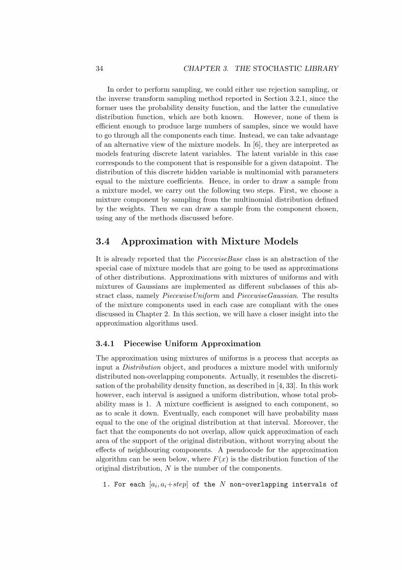
The approximation using mixtures of uniforms is a process that accepts asinput a Distribution object, and produces a mixture model with uniformlydistributed non-overlapping components. Actually, it resembles the discreti-sation of the probability density function, as described in [4, 33]. In this workhowever, each interval is assigned a uniform distribution, whose total prob-ability mass is 1. A mixture coefficient is assigned to each component, soas to scale it down. Eventually, each componet will have probability massequal to the one of the original distribution at that interval. Moreover, thefact that the components do not overlap, allow quick approximation of eacharea of the support of the original distribution, without worrying about theeffects of neighbouring components. A pseudocode for the approximationalgorithm can be seen below, where F (x) is the distribution function of theoriginal distribution, N is the number of the components.
1. For each [ai, ai+step] of the N non-overlapping intervals of

3.4. APPROXIMATION WITH MIXTURE MODELS 35
the support
2. weight← F (ai + step)− F (ai)
3. add U(ai, ai + step) and weight to the PiecewiseUniformresult
4. return PiecewiseUniform result
A more sophisticated algorithm could involve variable step size, or vari-able number of components. However, the current implementation is pre-ferred, since it has linear complexity. In fact, efficiency is a priority at thispoint, as the computation of the quantity F (ai) can prove rather expensive.More specifically, we have seen that the result of a binary operation will haveN2 components. This raw result should be re-approximated by a mixtureof N uniforms, in order to be used in future computations. We have seenin Equation (3.11) that the distribution function of a mixture model is acombination of the distribution functions of its components. Given that thecomponents are N2 in this case, it certainly makes sense to prefer efficientapproximation algorithms. Figure 3.6 depicts a simple example of approxi-mating the probability density function of a standard Gaussian distribution.
0
0.05
0.1
0.15
0.2
0.25
0.3
0.35
0.4
-5 -4 -3 -2 -1 0 1 2 3 4 5
N(0, 1)Approximation
Figure 3.6: Approximation of N(0, 1) using a mixture of 10 uniforms
36 CHAPTER 3. THE STOCHASTIC LIBRARY
3.4.2 Piecewise Gaussian Approximation
According to [2], a Gaussian mixture density can be used to approximateanother density function with arbitrary accuracy. The approximation usingmixtures of Gaussians is more complicated though, since the componentsshould overlap up to a certain extent, in order to successfully approximatesmooth density functions. Actually, there are several machine learning meth-ods for the task, the most popular of which is the Expectation-Maximisation(EM) algorithm [14]. The problem with most of the existing algorithmsthough, is that they are data oriented. In other words, they fit Gaussianmixture models to data, but what we need is to fit a mixture model to agiven density function. A very straightforward solution, and perhaps themost correct one, would be to produce a large dataset by sampling fromthe target distribution. Then we can apply an algorithm such as the EMto construct a mixture distribution that best explains the data produced.Nevertheless, given the fact that we want to perform computations in realtime, this is not an applicable solution at all.
An example of fitting mixtures of Gaussians directly to density functionscan be found in [19]. However, this solution is not efficient either, as it in-vloves searching over the 3N parameters of the Gaussian mixture (N means,N variances and N weights2). More specifically, a hill-climbing method isapplied, where each combination of parameters is tested by measuring thedistance from the original density, which is an expensive operation itself. Inany case, such an approach is not suitable for real time computations.
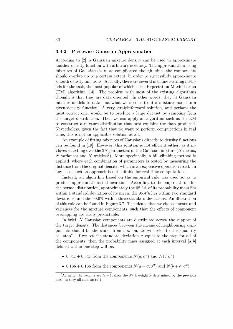
Instead, an algorithm based on the empirical rule was used so as toproduce approximations in linear time. According to the empirical rule forthe normal distribution, approximately the 68.2% of its probability mass lieswithin 1 standard deviation of its mean, the 95.4% lies within two standarddeviations, and the 99.6% within three standard deviations. An illustrationof this rule can be found in Figure 3.7. The idea is that we choose means andvariances for the mixture components, such that the effects of componentoverlapping are easily predictable.
In brief, N Gaussian components are distributed across the support ofthe target density. The distances between the means of neighbouring com-ponents should be the same; from now on, we will refer to this quantityas “step”. If we set the standard deviation σ equal to the step for all ofthe components, then the probability mass assigned at each interval [a, b]defined within one step will be:
• 0.341 + 0.341 from the components N(a, σ2) and N(b, σ2)
• 0.136 + 0.136 from the components N(a− σ, σ2) and N(b + σ, σ2)
2Actually, the weights are N − 1, since the N -th weight is determined by the previousones, as they all sum up to 1
3.4. APPROXIMATION WITH MIXTURE MODELS 37
Figure 3.7: Illustration of the empirical rule for the standard Gaussian dis-tribution
• 0.021 + 0.021 from the components N(a− 2σ, σ2) and N(b + 2σ, σ2)
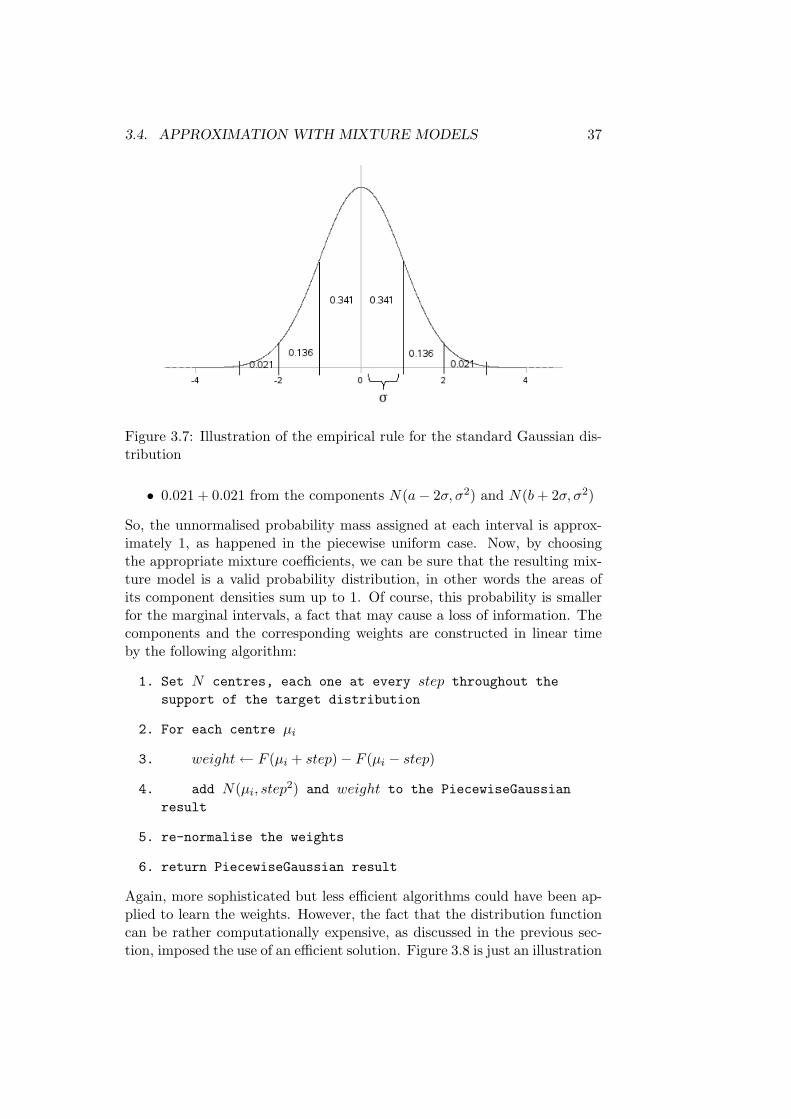
So, the unnormalised probability mass assigned at each interval is approx-imately 1, as happened in the piecewise uniform case. Now, by choosingthe appropriate mixture coefficients, we can be sure that the resulting mix-ture model is a valid probability distribution, in other words the areas ofits component densities sum up to 1. Of course, this probability is smallerfor the marginal intervals, a fact that may cause a loss of information. Thecomponents and the corresponding weights are constructed in linear timeby the following algorithm:
1. Set N centres, each one at every step throughout thesupport of the target distribution
2. For each centre µi
3. weight← F (µi + step)− F (µi − step)
4. add N(µi, step2) and weight to the PiecewiseGaussian
result
5. re-normalise the weights
6. return PiecewiseGaussian result
Again, more sophisticated but less efficient algorithms could have been ap-plied to learn the weights. However, the fact that the distribution functioncan be rather computationally expensive, as discussed in the previous sec-tion, imposed the use of an efficient solution. Figure 3.8 is just an illustration

38 CHAPTER 3. THE STOCHASTIC LIBRARY
of an approximation result. The accuracy is being improved, as we increasethe number of components, which is also verified in the evaluation section.
0
0.2
0.4
0.6
0.8
1
1.2
-1 -0.5 0 0.5 1 1.5
U(0, 1)Approximation
Figure 3.8: Approximation of U(0, 1) using a mixture of 10 Gaussians
3.5 Computations Using Mixture Models
Computations on random variables are implemented as overloaded C++ op-erators in the RandomVariable class. An operation on two random variablesinvolves the following steps:
i. Approximate the distributions of the input variables with mixtures ofN either uniform or Gaussian components.
ii. Apply the relevant computation at each pair of components. Each oneof these intermediate results will be weighted by the product of theweights of the components that is derived from.
iii. The resulting mixture density of N2 components will be approximatedas well, so as to be reduced to N mixture components.
It is straightforward to prove the validity of the second step for any kindof binary operator. For example, the resulting density of the sum X + Ywill be the convolution of the input densities, as defined in Equation (2.23).Since X and Y have mixture densities, we can plug (3.6) into (2.23) and

3.6. DEPENDENCY TRACKING MONTE CARLO 39
then we obtain:
(fX ∗ fY )(z) =∫ ∞
−∞
N∑i=1
wXifXi(z − y)N∑
j=1
wYjfYj (y)dy (3.12)
And if we pull the sums and the weights out of the integral, we obtain:
(fX ∗ fY )(z) =N∑
i=1
N∑j=1
wXiwYj
∫ ∞
−∞fXi(z − y)fYj (y)dy (3.13)
which is completely consistent with the description given in Step (ii) above,as the integrals in (3.13) are the densities of the sums of pairs of components.Since we are able to compute these quantities exactly, we can be sure that wehave no information loss at this step. The proofs for the remaining binaryoperations are similar. The intermediate results in each case of operationare computed as described in the relevant sections of Chapter 2.
3.6 Dependency Tracking Monte Carlo
In this section we discuss the implementation of the dependency trackingmechanism, and the way it is used in a Monte Carlo algorithm. It is notedthat the incorporation of this feature into the mixture model approximationapproach is a subject of future work.
The dependency information is recorded in the form of a directed graphof random variables. The edges in this graph are interpreted as parent-to-child relationships, where a parent is one of the inputs of a binary opera-tion, while a child is the resulting random variable. To put it differently,the arrows indicate the flow of computations. For convenience, the unaryoperations are considered as binary ones, whose second argument follows adelta distribution, a distribution whose density is described by the Dirac’sdelta function δ(x). In the same way, n–ary operations are treated as asuccessions of binary ones as well. For example, the expression: c = a +b + 2, will have the dependency graph depicted in Figure 3.9. It is notedthat the nodes that hold constants and intermediate results, are handled asrandom variables in terms of the graph only. They do not correspond toany RandomVariable object visible to the user.
A case that should also be examined is re-assignment of a distributionto a random variable, using an expression such as a = a + b or even a = b.While the user should not have access to the old distribution of the objecta anymore, its node in any existing dependency graph should remain un-changed, as there are other variables that depend on it. Instead, a new nodeshould be created that will point to the new value from now on. This policyalso ensures that if we change the distribution of a random variable, thiswill affect future computations only, not the past ones. In Figure 3.10, the
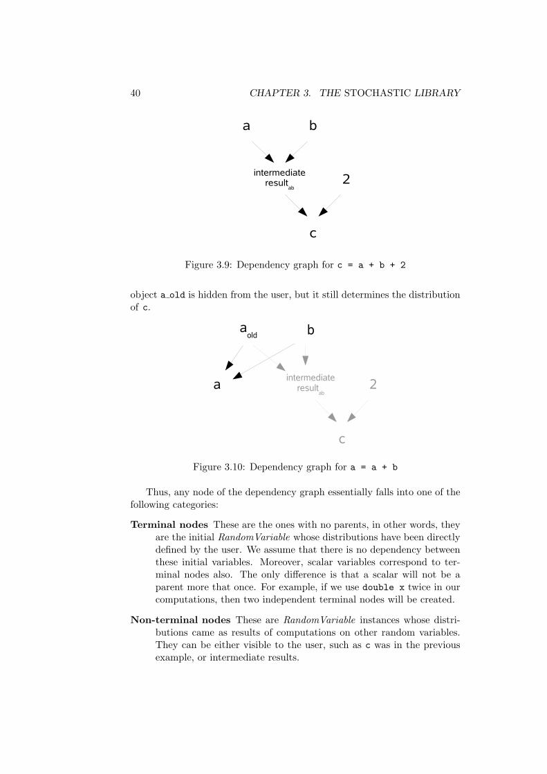
40 CHAPTER 3. THE STOCHASTIC LIBRARY
a
c
b
2intermediateresult
ab
Figure 3.9: Dependency graph for c = a + b + 2
object a old is hidden from the user, but it still determines the distributionof c.
aold
c
b
2intermediateresult
aba
Figure 3.10: Dependency graph for a = a + b
Thus, any node of the dependency graph essentially falls into one of thefollowing categories:
Terminal nodes These are the ones with no parents, in other words, theyare the initial RandomVariable whose distributions have been directlydefined by the user. We assume that there is no dependency betweenthese initial variables. Moreover, scalar variables correspond to ter-minal nodes also. The only difference is that a scalar will not be aparent more that once. For example, if we use double x twice in ourcomputations, then two independent terminal nodes will be created.
Non-terminal nodes These are RandomVariable instances whose distri-butions came as results of computations on other random variables.They can be either visible to the user, such as c was in the previousexample, or intermediate results.

3.6. DEPENDENCY TRACKING MONTE CARLO 41
What we have managed so far, is to express the dependencies as directedpaths in the graph. Each non-terminal node corresponds to a number of com-putational paths, let us refer to them as “personal computational graph”.Hence, a random variable will be dependent on all the elements of its per-sonal computational graph. Moreover, two non-terminal nodes that are notin the same path, will be also dependent if they have common elements intheir personal computational graphs. This structure is essentially a directedacyclic graph [48]. Moreover, all the non-terminal nodes have exactly twoedges pointing at them, since they are results of a specific binary operation.Thus, it is very straightforward to find the ancestors of a non-terminal nodeusing a simple depth-first-search algorithm, and consequently describe thedependency between any pair of random variables.
The Monte Carlo Implementation The information captured in thegraph can be used in order to develop a Monte Carlo algorithm that respectsthe dependencies that have been created by the computations. According tothe naıve Monte Carlo approach, a sample of the resulting distribution wouldbe drawn by just sampling from the distributions of the input variables, andthen apply the operator at this pair of samples. Eventually, the resultingdistribution is described by the empirical distribution function of the datasetproduced. In this implementation, the results are actually instances of theEmpiricalDistribution class discussed in Section 3.3.1.
Now, considering the example b = a + a, it is intuitive that this expres-sion should be equivalent to b = 2 * a, where a and b are RandomVariableobjects. In terms of the Monte Carlo approach, this implies that if the ob-ject a is already sampled, then it should not be sampled again. Instead,we should use the same sample at each sampling step, so as to simulate theoperation 2 * a.
Thus, the dependency tracking Monte Carlo involves a sampling processthat has access to the personal computational graph of each random variable.More accurately, each sampling step results in a recursive traversal of thepersonal computational graph. Coonsisely, if a random variable has beenalready sampled at a specific step, the same sample will be used in order toproduce the current sample of the resulting distribution. The algorithm ispresented in more detail in the following pseudocode.
1. Compute the binary operation betweenthe random variables X and Y
2. for N sampling steps
3. sample← recursive sampling(operator, X, Y )
4. add sample to the EmpiricalDistribution result
5. return EmpiricalDistribution result

42 CHAPTER 3. THE STOCHASTIC LIBRARY
The function recursive sampling returns one sample for the resulting ran-dom variable of the expression operator(X, Y ).
1. recursive sampling(operator, X, Y )
2. if X is sampled
3. sampleX ← retrieve the sample of X
4. else if X is a terminal node
5. sampleX ← sample(X)
6. else if X is a non-terminal node
7. X1, X2 ← parrents of X
8. sampleX ← recursive sampling(operationX, X1, X2)
9. if Y is sampled
10. sampleY ← retrieve the sample of Y
11. else if Y is a terminal node
12. sampleY ← sample(Y )
13. else if Y is a non-terminal node
14. Y1, Y2 ← parrents of Y
15. sampleY ← recursive sampling(operationY , Y1, Y2)
16. return operation(sampleX , sampleY )
3.7 General Remarks on the Implementation
The implementation so far includes 20 classes in 3500 source lines of codeapproximately. The classes that the users should be aware of, have beenalready outlined in Section 3.1. Consisely, the users are supposed to initialiseobjects of the RandomVariable class, using instances of distribution classes.Once a RandomVariable object is assigned a distribution, it can be eitherqueried on its distribution or used in computations. However, there is also anumber of distribution classes that are not accessible by the user. Those areused to hold intermediate results during a computation. Such an exampleis the sum of two uniforms, as defined in Section 2.3.2.

3.7. GENERAL REMARKS ON THE IMPLEMENTATION 43
Informatics Research Proposal Timeline Eventually, it is worth re-viewing the project’s timeline, as it was defined in terms of the research pro-posal. In Table 3.1, we can see the tasks that the project was divided into,and their associated starting and completion dates. Although the projectwas on schedule, we have to note that the implementation sub-tasks as ini-tially recorded do not reflect the reality. Originally, the implementationsub-tasks were supposed to correspond to specific C modules. However, ithas been decided that the implementation language would change from Cto C++, so as to adopt the principles of object-oriented programming. Thisdecision not only improved the code resuability and maintainability, but alsomade the use of the library more intuitive. This change of plans had a majoreffect in the architecture of the system though, as many of the modules werespread across a number of classes.
Task Start FinishResearching 18 May 18 MaySpecification 25 May 30 MayImplementation 1 Jun 8 AugMonte Carlo simulation 1 Jun 13 JunSkeleton component 1 Jun 13 JunApproximating components 15 Jun 4 JulOperators 6 Jul 28 JulDependency tracking 20 Jul 8 AugTesting 8 Jun 8 AugPerform evaluation experiments 27 Jul 15 AugWriting 22 Jun 20 Aug
Table 3.1: Project tasks, starting and completion dates

44 CHAPTER 3. THE STOCHASTIC LIBRARY

Chapter 4
Evaluation
The evaluation of our approach mainly involves comparisons between prob-ability distributions. In fact, the resulting distributions given by our imple-mentation for each kind of operator are compared with the theoretical ones,when these are available. In case the theoretical results cannot be analyti-cally computed, we use a Monte Carlo approach featuring 1 million samplesas reference. After all, is is reasonable to expect that the more we increasethe number of samples, the more accurate the Monte Carlo results will be.In order to completely define the notion of comparison between probabilitydistributions, we introduce a number of similarity measures in Section 4.1.
In this project, we have actually implemented two different approachesthat deal with the problem of performing arithmetic operations on randomvariables, including approximation with mixtures of models and dependencytracking Monte Carlo. As we have seen, the first method involves two al-ternatives as components for the approximating mixture models. So, thepurpose of the evaluation of this method is not only to have a picture of thequality of the computations for each one of them independently, but also tomake comparisons between them. Both accuracy and efficiency are issuesfor the mixture model approximation, so both the distances between thedistributions and the running times will be displayed. Of course, the run-ning times are just indicative. It is noted though that the experiments havebeen conducted in an Intel R© CoreTM2 Duo T8300 @ 2.40GHz PC runningLinux.
On the other hand, efficiency is not of great concern for dependencytracking Monte Carlo. The evaluation of this method should focus on itsability to capture the dependencies that arise through out the computations.Thus the method will be compared against series of computations that canbe easily tracked to verify the correct result. The purpose will be to verifythat the results given are consistent with the dependencies involved.
45
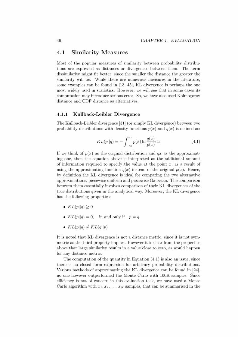
46 CHAPTER 4. EVALUATION
4.1 Similarity Measures
Most of the popular measures of similarity between probability distribu-tions are expressed as distances or divergences between them. The termdissimilarity might fit better, since the smaller the distance the greater thesimilarity will be. While there are numerous measures in the literature,some examples can be found in [13, 45], KL divergence is perhaps the onemost widely used in statistics. However, we will see that in some cases itscomputation may introduce serious error. So, we have also used Kolmogorovdistance and CDF distance as alternatives.
4.1.1 Kullback-Leibler Divergence
The Kullback-Leibler divergence [31] (or simply KL divergence) between twoprobability distributions with density functions p(x) and q(x) is defined as:
KL(p||q) = −∫ ∞
−∞p(x) ln
q(x)p(x)
dx (4.1)
If we think of p(x) as the original distribution and qx as the approximat-ing one, then the equation above is interpreted as the additional amountof information required to specify the value at the point x, as a result ofusing the approximating function q(x) instead of the original p(x). Hence,by definition the KL divergence is ideal for comparing the two alternativeapproximations, piecewise uniform and piecewise Gaussian. The comparisonbetween them essentially involves comparison of their KL divergences of thetrue distributions given in the analytical way. Moreover, the KL divergencehas the following properties:
• KL(p||q) ≥ 0
• KL(p||q) = 0, in and only if p = q
• KL(p||q) 6= KL(q||p)
It is noted that KL divergence is not a distance metric, since it is not sym-metric as the third property implies. However it is clear from the propertiesabove that large similarity results in a value close to zero, as would happenfor any distance metric.
The computation of the quantity in Equation (4.1) is also an issue, sincethere is no closed form expression for arbitrary probability distributions.Various methods of approximating the KL divergence can be found in [24],no one however outperformed the Monte Carlo with 100K samples. Sinceefficiency is not of concern in this evaluation task, we have used a MonteCarlo algorithm with x1, x2, . . . , xN samples, that can be summarised in the
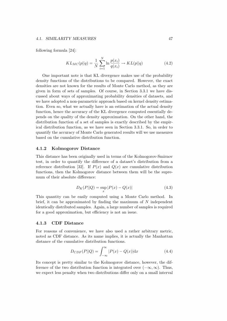
4.1. SIMILARITY MEASURES 47
following formula [24]:
KLMC(p||q) =1N
N∑i=1
lnp(xi)q(xi)
→ KL(p||q) (4.2)
One important note is that KL divergence makes use of the probabilitydensity functions of the distributions to be compared. However, the exactdensities are not known for the results of Monte Carlo method, as they aregiven in form of sets of samples. Of course, in Section 3.3.1 we have dis-cussed about ways of approximating probability densities of datasets, andwe have adopted a non-parametric approach based on kernel density estima-tion. Even so, what we actually have is an estimation of the actual densityfunction, hence the accuracy of the KL divergence computed essentially de-pends on the quality of the density approximation. On the other hand, thedistribution function of a set of samples is exactly described by the empir-ical distribution function, as we have seen in Section 3.3.1. So, in order toquantify the accuracy of Monte Carlo generated results will we use measuresbased on the cumulative distribution function.
4.1.2 Kolmogorov Distance
This distance has been originally used in terms of the Kolmogorov-Smirnovtest, in order to quantify the difference of a dataset’s distribution from areference distribution [32]. If P (x) and Q(x) are cumulative distributionfunctions, then the Kolmogorov distance between them will be the supre-mum of their absolute difference:
DK(P ||Q) = supx|P (x)−Q(x)| (4.3)
This quantity can be easily computed using a Monte Carlo method. Inbrief, it can be approximated by finding the maximum of N independentidentically distributed samples. Again, a large number of samples is requiredfor a good approximation, but efficiency is not an issue.
4.1.3 CDF Distance
For reasons of convenience, we have also used a rather arbitrary metric,noted as CDF distance. As its name implies, it is actually the Manhattandistance of the cumulative distribution functions.
DCDF (P ||Q) =∫ ∞
−∞|P (x)−Q(x)|dx (4.4)
Its concept is pretty similar to the Kolmogorov distance, however, the dif-ference of the two distribution function is integrated over (−∞,∞). Thus,we expect less penalty when two distributions differ only on a small interval
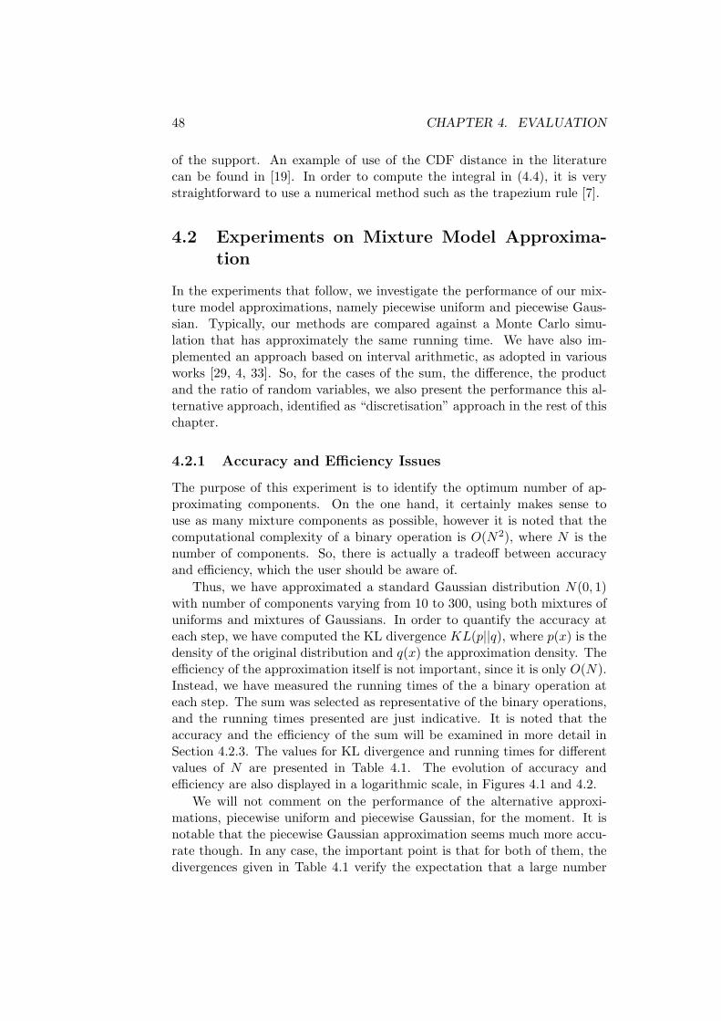
48 CHAPTER 4. EVALUATION
of the support. An example of use of the CDF distance in the literaturecan be found in [19]. In order to compute the integral in (4.4), it is verystraightforward to use a numerical method such as the trapezium rule [7].
4.2 Experiments on Mixture Model Approxima-tion
In the experiments that follow, we investigate the performance of our mix-ture model approximations, namely piecewise uniform and piecewise Gaus-sian. Typically, our methods are compared against a Monte Carlo simu-lation that has approximately the same running time. We have also im-plemented an approach based on interval arithmetic, as adopted in variousworks [29, 4, 33]. So, for the cases of the sum, the difference, the productand the ratio of random variables, we also present the performance this al-ternative approach, identified as “discretisation” approach in the rest of thischapter.
4.2.1 Accuracy and Efficiency Issues
The purpose of this experiment is to identify the optimum number of ap-proximating components. On the one hand, it certainly makes sense touse as many mixture components as possible, however it is noted that thecomputational complexity of a binary operation is O(N2), where N is thenumber of components. So, there is actually a tradeoff between accuracyand efficiency, which the user should be aware of.
Thus, we have approximated a standard Gaussian distribution N(0, 1)with number of components varying from 10 to 300, using both mixtures ofuniforms and mixtures of Gaussians. In order to quantify the accuracy ateach step, we have computed the KL divergence KL(p||q), where p(x) is thedensity of the original distribution and q(x) the approximation density. Theefficiency of the approximation itself is not important, since it is only O(N).Instead, we have measured the running times of the a binary operation ateach step. The sum was selected as representative of the binary operations,and the running times presented are just indicative. It is noted that theaccuracy and the efficiency of the sum will be examined in more detail inSection 4.2.3. The values for KL divergence and running times for differentvalues of N are presented in Table 4.1. The evolution of accuracy andefficiency are also displayed in a logarithmic scale, in Figures 4.1 and 4.2.
We will not comment on the performance of the alternative approxi-mations, piecewise uniform and piecewise Gaussian, for the moment. It isnotable that the piecewise Gaussian approximation seems much more accu-rate though. In any case, the important point is that for both of them, thedivergences given in Table 4.1 verify the expectation that a large number

4.2. EXPERIMENTS ON MIXTURE MODEL APPROXIMATION 49
Number ofComponents
Piecewise Uniform Piecewise GaussianKL
DivergenceTime(ms)
KLDivergence
Time(ms)
10 0.02509870 0.2 0.05845930 0.230 0.00292771 2.9 0.00119073 2.660 0.00069225 20 0.00004625 1580 0.00030220 50 0.00002190 30100 0.00004645 100 0.00001575 60120 0.00001380 200 0.00000862 110150 0.00001045 600 0.00000789 220180 0.00001022 1610 0.00000643 440200 0.00000894 2510 0.00000552 800220 0.00000514 3420 0.00000316 1300250 0.00000483 4980 0.00000172 2280300 0.00000344 8900 0.00000059 4050
Table 4.1: KL divergence and running times for varying number of compo-nents
-16
-14
-12
-10
-8
-6
-4
-2
0 50 100 150 200 250 300
Piecewise UniformPiecewise Gaussian
3
3
33
3
3 33 3 3
3 3 3 3 33
3
3
3
Figure 4.1: KL divergence in a logarithmic scale, for different number ofcomponents

50 CHAPTER 4. EVALUATION
-2
0
2
4
6
8
10
0 50 100 150 200 250 300
Piecewise UniformPiecewise Gaussian
3
3
33
33 3
33 3 3
33
33
33
33
Figure 4.2: Running times (ms) in a logarithmic scale, for different numberof components
of componets results in better accuracy. It is also noted that the MonteCarlo method used to approximate the KL divergence (Section 4.1.1), wasquite unstable for more than 200 components. In fact, these values were soclose to zero, that we had to use more than 1 million samples to obtain agood approximation at each case. On the other hand, we can see that therunning times seem to be increased in a quadratic manner. This is actuallyconsistent with the O(N2) complexity of the algorithm used.
Eventually, the accuracy granted for 100 components seems acceptable,while the running time usually remains below 100 milliseconds, which meansthat it is feasible to be used for a series of computations. For the rest of thischapter, the number of components is set to 100, unless stated otherwise.
4.2.2 Performance for Unary Operations
The unary operations are actually functions of one random variable, as de-fined in Section 2.2. They are certainly less interesting than the binary ones,since their complexity is only O(N), however we still need to validate the as-sumptions we have made so far. It is also noted that from this point and on,we will make use of all the measures of performance at our disposal, includ-ing Kolmogorov and CDF distance and running times. The KL divergencewill be computed for non-Monte Carlo derived distributions only.

4.2. EXPERIMENTS ON MIXTURE MODEL APPROXIMATION 51
Method
Similarity to True Distribution
KLDivergence
KolmogorovDistance
CDFDistance
Time(ms)
Monte Carlo (2K) N/A 0.0126734 0.0133106 120Piecewise Uniform 0.0002347 0.0001985 0.0002928 1.4Piecewise Gaussian 0.0001788 0.0028174 0.0065224 1.4
Table 4.2: Performance for −1/2X + 4, where X ∼ N(−4, 2)
Linear Function of a Random Variable
The current example involves estimating the expression Y = aX + b, wherea = −1/2, b = 4 and X ∼ N(−4, 2). According to what we have seen inSection 2.2.1, we know that the true resulting distribution will be of theform N(aµX + b, σ2a2). In this case, the distribution of the result will beN(6, 0.5).
In Table 4.2 we can see that both piecewise uniform and piecewise Gaus-sian approach outperformed the simple Monte Carlo featuring 2000 samples.Moreover, the operation was carried out in about 1 millisecond in both cases.Of course, that was expected form an operation with linear complexity.
Maximum of a Random Variable and a Constant
We will now try to approximate the result of the expression max(X, a),where a = 3 and X ∼ N(4, 1). Since the constant a falls within the sup-port of the distribution of X, the result will be a distribution that is bothcontinuous and discrete, according to the discussion in Section 2.2.3. Thereference result in this case will be produced by Monte Carlo using 100Ksamples. The performance measures for the different approaches are listedin Table 4.3.
Surprisingly enough, the Kolmogorov distances imply that the MonteCarlo with 2000 samples is more accurate than both of our mixture modelsapproximations. On the other hand, the CDF distances indicate that mix-ture model approaches are much more accurate. This disagreement shouldbe attributed to the tendency that the Kolmogorov distance has to penalisetoo much any large divergence, even if it only exists in a very small area ofthe support. In our case, we can see in Figure 4.3 that this happens in thearea close to 3, as this is the discrete component of the mixed distribution,which has been approximated by a Gaussian spike. Thus, the informationloss should be attributed to the re-approximation of the resulting distri-bution, as our approximating algorithms described in Section 3.4 tend tosmooth the sharp areas of a density function.
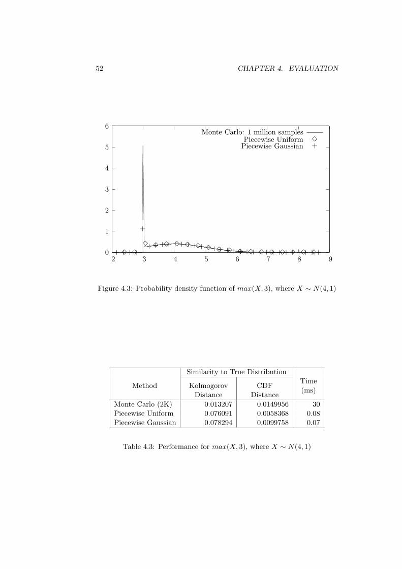
52 CHAPTER 4. EVALUATION
0
1
2
3
4
5
6
2 3 4 5 6 7 8 9
Monte Carlo: 1 million samplesPiecewise Uniform
3 3
3 3 3 3 3 3 3 3 3 3 3 3 3 3 3 3 3
3Piecewise Gaussian
++++
+
+++++++++++++++++++++++++++
+
Figure 4.3: Probability density function of max(X, 3), where X ∼ N(4, 1)
Method
Similarity to True Distribution
KolmogorovDistance
CDFDistance
Time(ms)
Monte Carlo (2K) 0.013207 0.0149956 30Piecewise Uniform 0.076091 0.0058368 0.08Piecewise Gaussian 0.078294 0.0099758 0.07
Table 4.3: Performance for max(X, 3), where X ∼ N(4, 1)
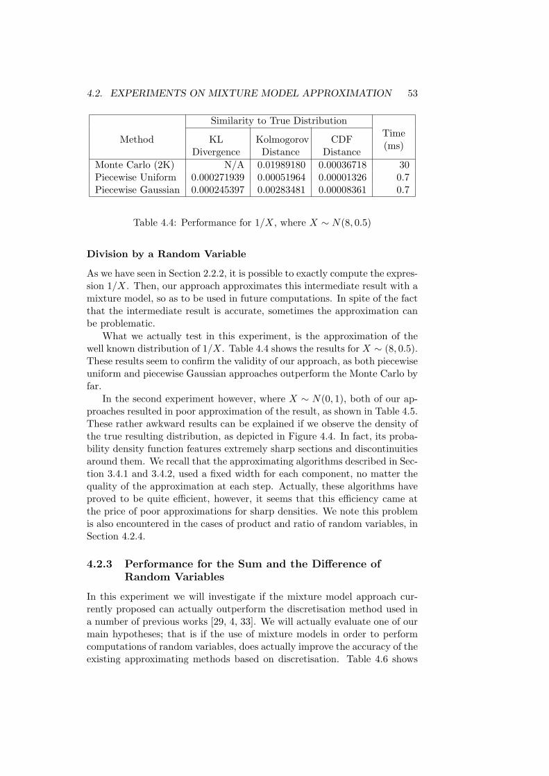
4.2. EXPERIMENTS ON MIXTURE MODEL APPROXIMATION 53
Method
Similarity to True Distribution
KLDivergence
KolmogorovDistance
CDFDistance
Time(ms)
Monte Carlo (2K) N/A 0.01989180 0.00036718 30Piecewise Uniform 0.000271939 0.00051964 0.00001326 0.7Piecewise Gaussian 0.000245397 0.00283481 0.00008361 0.7
Table 4.4: Performance for 1/X, where X ∼ N(8, 0.5)
Division by a Random Variable
As we have seen in Section 2.2.2, it is possible to exactly compute the expres-sion 1/X. Then, our approach approximates this intermediate result with amixture model, so as to be used in future computations. In spite of the factthat the intermediate result is accurate, sometimes the approximation canbe problematic.
What we actually test in this experiment, is the approximation of thewell known distribution of 1/X. Table 4.4 shows the results for X ∼ (8, 0.5).These results seem to confirm the validity of our approach, as both piecewiseuniform and piecewise Gaussian approaches outperform the Monte Carlo byfar.
In the second experiment however, where X ∼ N(0, 1), both of our ap-proaches resulted in poor approximation of the result, as shown in Table 4.5.These rather awkward results can be explained if we observe the density ofthe true resulting distribution, as depicted in Figure 4.4. In fact, its proba-bility density function features extremely sharp sections and discontinuitiesaround them. We recall that the approximating algorithms described in Sec-tion 3.4.1 and 3.4.2, used a fixed width for each component, no matter thequality of the approximation at each step. Actually, these algorithms haveproved to be quite efficient, however, it seems that this efficiency came atthe price of poor approximations for sharp densities. We note this problemis also encountered in the cases of product and ratio of random variables, inSection 4.2.4.
4.2.3 Performance for the Sum and the Difference ofRandom Variables
In this experiment we will investigate if the mixture model approach cur-rently proposed can actually outperform the discretisation method used ina number of previous works [29, 4, 33]. We will actually evaluate one of ourmain hypotheses; that is if the use of mixture models in order to performcomputations of random variables, does actually improve the accuracy of theexisting approximating methods based on discretisation. Table 4.6 shows

54 CHAPTER 4. EVALUATION
0
0.05
0.1
0.15
0.2
0.25
0.3
-25 -20 -15 -10 -5 0 5 10 15 20 25
1/XPiecewise Uniform
3333333333333333
3
3
3
3
3
3333333333333333
3Piecewise Gaussian
++++++++++++++++
+
+
+
+
+
++++++++++++++++
+
Figure 4.4: Probability density function of 1/X, where X ∼ N(0, 1)
Method
Similarity to True Distribution
KLDivergence
KolmogorovDistance
CDFDistance
Time(ms)
Monte Carlo (2K) N/A 0.017782 2.20295 30Piecewise Uniform 0.038805 0.020362 0.68778 0.7Piecewise Gaussian 0.204265 0.048501 0.68955 0.7
Table 4.5: Performance for 1/X, where X ∼ N(0, 1)

4.2. EXPERIMENTS ON MIXTURE MODEL APPROXIMATION 55
Method
Similarity to True Distribution
KLDivergence
KolmogorovDistance
CDFDistance
Time(ms)
Monte Carlo (10K) N/A 0.0122061 0.0361947 100Discretisation 0.000387272 0.0005758 0.0022914 60Piecewise Uniform 0.000354792 0.0005086 0.0019316 100Piecewise Gaussian 0.000180433 0.0025144 0.0141960 60
Table 4.6: Performance for X + Y , where X ∼ N(2, 1) and Y ∼ N(3, 2)
the results for two normally distributed random variables, X ∼ N(2, 1) andY ∼ N(3, 2). The true resulting distribution will be N ∼ (5, 3).
Again the Monte Carlo exhibits the poorest performance, according toall of the accuracy measures. The most remarkable result though, is thatthe mixture of uniforms approach appears to be more accurate than thediscretisation approach discussed in the literature. However, this improve-ment in terms of accuracy is not for free at all. The running times of forthe sum using piecewise uniform approximation is approximately 30 or 40milliseconds slower that the discretisation method. This was more or lessexpected, as the computation of the actual sum of uniforms is essentially anexpensive operation, which is repeated N2 times. On the other hand, thecomputation of the intermediate result for the piecewise Gaussian method,involves just the creation of the resulting normal distribution, which makesthe whole process more efficient.
Another interesting finding is the fact that not all accuracy measuresagree on the approximation quality of piecewise Gaussian. The KL di-vergence indicates that the sum is more accurately approximated using aGaussian mixture, while on the other hand, distance measures based on thecumulative distribution function seem to favour the piecewise uniform ap-proach. This issue is further investigated in Section 4.2.6, where we examinethe error propagation.
The difference is also covered in this section. The implementation of thesum and the difference of random variables is equivalent, since the differenceX − Y is defined as the sum X + (−Y ), as discussed in Section 2.3.
4.2.4 Performance for the Product and the Ratio ofRandom Variables
As we have discussed in Section 2.4, there is no closed form expression forthe product and the ration of random variables, even for simple distribu-tions. For the piecewise uniform approach, the intermediate results for bothproduct and ratio were approximated by uniforms, as an efficient substi-

56 CHAPTER 4. EVALUATION
Method
Similarity to True Distribution
KolmogorovDistance
CDFDistance
Time(ms)
Monte Carlo (5K) 0.017146 0.110625 60Discretisation 0.005952 0.064949 60Piecewise Gaussian 0.001606 0.013265 60
Table 4.7: Performance for XY , where X ∼ U(2, 6) and Y ∼ N(3, 0.5)
Method
Similarity to True Distribution
KolmogorovDistance
CDFDistance
Time(ms)
Monte Carlo (5K) 0.010158 0.036066 60Discretisation 0.018202 0.025796 60Piecewise Gaussian 0.059393 0.158304 60
Table 4.8: Performance for XY , where X ∼ N(−1, 2) and Y ∼ N(0, 1)
tute of the true product and ratio of uniform distributions. In fact, theseare the only cases of operations implemented according to the discretisationapproach. On the other hand, the product and the ratio for the piecewiseGaussian approach (sections 2.4.1 and 2.4.2), are supposed to approximatebetter the intermediate and hopefully the final results. That remains tobe seen by comparing these alternative approaches using a Monte Carloapproach of 1 million samples as reference.
Tables 4.7 and 4.8 list the product results for different examples. Giventhe running times observed, the two alternative methods have almost identi-cal efficiency in both examples. This was pretty much expected, if we thinkof the way the intermediate results are produced. Now, in the first example,where X ∼ U(2, 6) and Y ∼ N(3, 0.5), piecewise Gaussian approximationseems to achieve considerably better accuracy than the piecewise uniformapproach. Our assumption that a better approximation of the intermediateresult would improve the accuracy is actually confirmed in this experiment.
However, the second experiment, is actually an example of poor perfor-mance of the current implementation. For X ∼ N(−1, 2) and Y ∼ N(0, 1),the resulting distribution has a high probability spike in the area close tozero. This area is poorly approximated by both approaches, as we can evensee in Figure 4.5. It is also notable that the simple Monte Carlo methodexhibits higher accuracy in this case.
As happened with the product, the performance for the ratio of random

4.2. EXPERIMENTS ON MIXTURE MODEL APPROXIMATION 57
0
0.1
0.2
0.3
0.4
0.5
0.6
0.7
0.8
0.9
1
-25 -20 -15 -10 -5 0 5 10 15 20 25
Monte Carlo: 1 million samplesDiscretisation
33333333333333333
3
3
33
3333333333333333
3Piecewise Gaussian
+++++++++++++++++
+
+
+
+++++++++++++++++
+
Figure 4.5: Probability density function of XY , where X ∼ N(−1, 2) andY ∼ N(0, 1)
Method
Similarity to True Distribution
KolmogorovDistance
CDFDistance
Time(ms)
Monte Carlo (5K) 0.014614 0.00217576 60Discretisation 0.008510 0.00194967 60Piecewise Gaussian 0.005199 0.00097181 60
Table 4.9: Performance for X/Y , where X ∼ U(2, 6) and Y ∼ U(9, 11)
variables tends to be poorer if the true resulting has discontinuous highprobability areas. Again, we present examples that illustrate both cases.The first example, whose results are outlined in Table 4.9, clearly indicatesthat the piecewise Gaussian approach is more accurate.
In the second example, where X ∼ N(1, 1) and Y ∼ N(0, 1), the prob-ability density function of the ratio is shown in Figure 4.6. Given thatthe currently used algorithms do not produce accurate enough approxima-tions of such sharp density functions, the poor performance of the piecewiseGaussian shown in Table 4.10 was rather expected. It is important though,that the discretisation approach performed badly as well. Judging by itsshape, it is obvious that the most of the 100 components approximate thelow probability tails. The probability peak near zero, which is the most in-
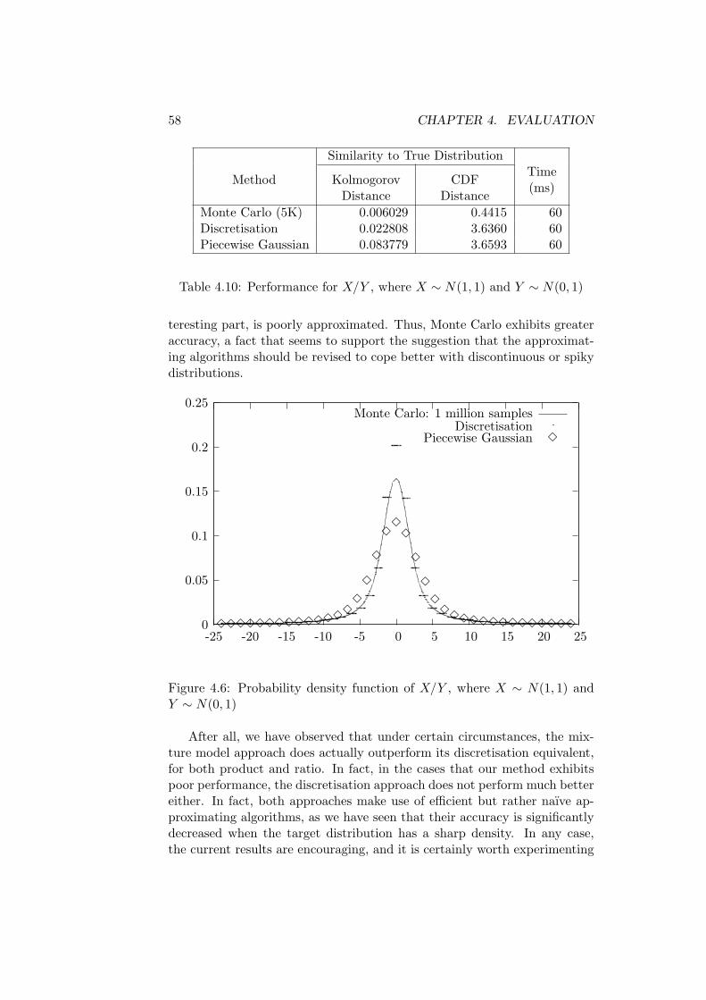
58 CHAPTER 4. EVALUATION
Method
Similarity to True Distribution
KolmogorovDistance
CDFDistance
Time(ms)
Monte Carlo (5K) 0.006029 0.4415 60Discretisation 0.022808 3.6360 60Piecewise Gaussian 0.083779 3.6593 60
Table 4.10: Performance for X/Y , where X ∼ N(1, 1) and Y ∼ N(0, 1)
teresting part, is poorly approximated. Thus, Monte Carlo exhibits greateraccuracy, a fact that seems to support the suggestion that the approximat-ing algorithms should be revised to cope better with discontinuous or spikydistributions.
0
0.05
0.1
0.15
0.2
0.25
-25 -20 -15 -10 -5 0 5 10 15 20 25
Monte Carlo: 1 million samplesDiscretisation
Piecewise Gaussian
33333333333333
3
3
3
33
3
3
3
33
3333333333333
3
Figure 4.6: Probability density function of X/Y , where X ∼ N(1, 1) andY ∼ N(0, 1)
After all, we have observed that under certain circumstances, the mix-ture model approach does actually outperform its discretisation equivalent,for both product and ratio. In fact, in the cases that our method exhibitspoor performance, the discretisation approach does not perform much bettereither. In fact, both approaches make use of efficient but rather naıve ap-proximating algorithms, as we have seen that their accuracy is significantlydecreased when the target distribution has a sharp density. In any case,the current results are encouraging, and it is certainly worth experimenting

4.2. EXPERIMENTS ON MIXTURE MODEL APPROXIMATION 59
with more sophisticated approximating algorithms.
4.2.5 Performance for the Minimum and the Maximum ofRandom Variables
The implementations of both minimum and maximum of random variablesmake use of the exact results, as described in Section 2.5. Eventually, thetheoretical results are approximated with mixture models. So, we haveavoided the N2 steps of the other binary operations, a fact that explainsthe high efficiency achieved for the current ones. In the first example, wherex ∼ N(0, 1) and Y ∼ N(−1, 8), we have also achieved high levels of accuracyfor both mixture model approximations. It is noted that the similarity mea-sures, which are presented in Table 4.11, are with respect to the theoreticalresult.
In the second example summarised in Table 4.12, we have computed theminimum of two exponentially distributed variables, X ∼ Exp(2) and Y ∼Exp(3). It is known that their minimum will follow exponential distributionExp(λ) with parameter λ = λX + λY . This falls in the case of densitiesthat have discontinuities at high probability areas, which has been alreadyidentified as problematic for our system. In Figure 4.7, we can see thatthe result is poorly approximated by the Gaussian mixture near the areaof discontinuity. On the other hand, the piecewise uniform approximationseems less affected, a fact also verified by the similarity measures recorded.
0
0.5
1
1.5
2
2.5
3
3.5
4
4.5
5
-0.5 0 0.5 1 1.5 2
Exp(5)Piecewise Uniform
Piecewise Gaussian
3 3 3
3
3
3
3
33
3 3 3 3 3 3 3 3 3 3 3 3 3 3 3
3
Figure 4.7: Probability density function of min(X, Y ), where X ∼ Exp(2)and Y ∼ Exp(3)

60 CHAPTER 4. EVALUATION
Method
Similarity to True Distribution
KLDivergence
KolmogorovDistance
CDFDistance
Time(ms)
Monte Carlo (2K) N/A 0.0216223 0.0526379 20Piecewise Uniform 0.00049898 0.0005259 0.0011792 0.06Piecewise Gaussian 0.00016757 0.0022473 0.0072830 0.06
Table 4.11: Performance for max(X, Y ), where x ∼ N(0, 1) and Y ∼N(−1, 8)
Method
Similarity to True Distribution
KLDivergence
KolmogorovDistance
CDFDistance
Time(ms)
Monte Carlo (2K) N/A 0.0203852 0.00474036 20Piecewise Uniform 0.0001100 0.0008231 0.00035788 0.06Piecewise Gaussian 0.0349908 0.0373825 0.00860947 0.06
Table 4.12: Performance for min(X, Y ), where X ∼ Exp(2) and Y ∼ Exp(3)
4.2.6 Error Propagation
Since our method involves approximation of the actual result, this essentiallyentails some error. From what we have seen so far, at least in the case ofsmooth resulting densities, our approach tends to produce smaller error thanthe simple Monte Carlo method, or the discretisation method used in theliterature so far [29, 4, 33]. However, it is worth investigating how this errorevolves in a series of computations. The experiment conducted in order toestimate the error propagation, is outlined by the following steps:
i. Pick a normally distributed random variable X ∼ N(µX , σ2X), with
random parameters
ii. Pick a normally distributed random variable Y ∼ N(µY , σ2Y ), with
random parameters
iii. Keep the result Y ← X + Y and go to Step (ii).
This procedure has been applied to the piecewise uniform, the piecewiseGaussian and the discretisation approach. Figure 4.8 depicts the evolutionof the error as captured by the KL divergence between the original resultand the results given by the different methods.
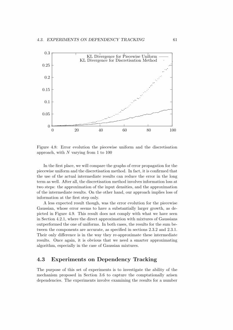
4.3. EXPERIMENTS ON DEPENDENCY TRACKING 61
0
0.05
0.1
0.15
0.2
0.25
0.3
0 20 40 60 80 100
KL Divergence for Piecewise UniformKL Divergence for Discretisation Method
Figure 4.8: Error evolution the piecewise uniform and the discretisationapproach, with N varying from 1 to 100
In the first place, we will compare the graphs of error propagation for thepiecewise uniform and the discretisation method. In fact, it is confirmed thatthe use of the actual intermediate results can reduce the error in the longterm as well. After all, the discretisation method involves information loss attwo steps: the approximation of the input densities, and the approximationof the intermediate results. On the other hand, our approach implies loss ofinformation at the first step only.
A less expected result though, was the error evolution for the piecewiseGaussian, whose error seems to have a substantially larger growth, as de-picted in Figure 4.9. This result does not comply with what we have seenin Section 4.2.1, where the direct approximation with mixtures of Gaussiansoutperformed the one of uniforms. In both cases, the results for the sum be-tween the components are accurate, as specified in sections 2.3.2 and 2.3.1.Their only difference is in the way they re-approximate these intermediateresults. Once again, it is obvious that we need a smarter approximatingalgorithm, especially in the case of Gaussian mixtures.
4.3 Experiments on Dependency Tracking
The purpose of this set of experiments is to investigate the ability of themechanism proposed in Section 3.6 to capture the comptationally arisendependencies. The experiments involve examining the results for a number

62 CHAPTER 4. EVALUATION
0
0.02
0.04
0.06
0.08
0.1
0.12
0.14
0.16
0.18
0.2
0 5 10 15 20
KL Divergence for Piecewise Gaussian
Figure 4.9: Error evolution the piecewise Gaussian approach, with N varyingfrom 1 to 20
of simple expressions that imply dependency of the input variables.In the algebra of random variables, variables that follow the same distri-
bution are not essentially supposed to be equal. For example, if X ∼ N(0, 1)and Y ∼ N(0, 1), the result of X + Y would follow a normal distributionN(0, 2), as we have seen in Section 2.3. On the other hand, the distributionof the resulting distribution of 2X would be N(0, 4), since we apply a linearfunction (Section 2.2.1). Moreover, it would be reasonable that the expres-sion 2X decomposed into X +X. The inequality between X +Y and X +Xcan be explained if we observe that in the second case, the variables are notindependent at all. That is the kind of dependency the tracking mechanismis supposed to follow. In Figure 4.10, we present the resulting densities ofthese expressions, as given by our Monte Carlo implementation.
Another very intuitive example is the computation of the expressionsX −X and X − Y , where X and Y are independent random variables. Forconvenience, let be X ∼ N(0, 1) and Y ∼ N(0, 1). The distribution of thedifference of these independent Gaussians will be N(0, 2), while it is quiteobvious that the in the case of X − X the result should be zero in anycase. These are exactly the densities derived using the dependency trackingMonte Carlo approach, as depicted in Figure 4.11.
Finally, the expression XY/X should give Y as result, but it is not thesame in the case of XY/Z for independent X and Z that follow the same dis-tribution. The results are displayed in Figure 4.12. Yet again, it is confirmed

4.3. EXPERIMENTS ON DEPENDENCY TRACKING 63
0
0.05
0.1
0.15
0.2
0.25
0.3
-8 -6 -4 -2 0 2 4 6 8
2XX + X
3 3 3 3 33
3
3
3
3
3
33
3
3
3
3
3
33
3 3 3 3 3
3X + Y
Figure 4.10: Probability density functions of 2X, X + X and X + Y , whereX ∼ N(0, 1) and Y ∼ N(0, 1)
0
0.2
0.4
0.6
0.8
1
-6 -4 -2 0 2 4 6
X −XX − Y
Figure 4.11: Probability density functions of X − X and X − Y , whereX ∼ N(0, 1) and Y ∼ N(0, 1)
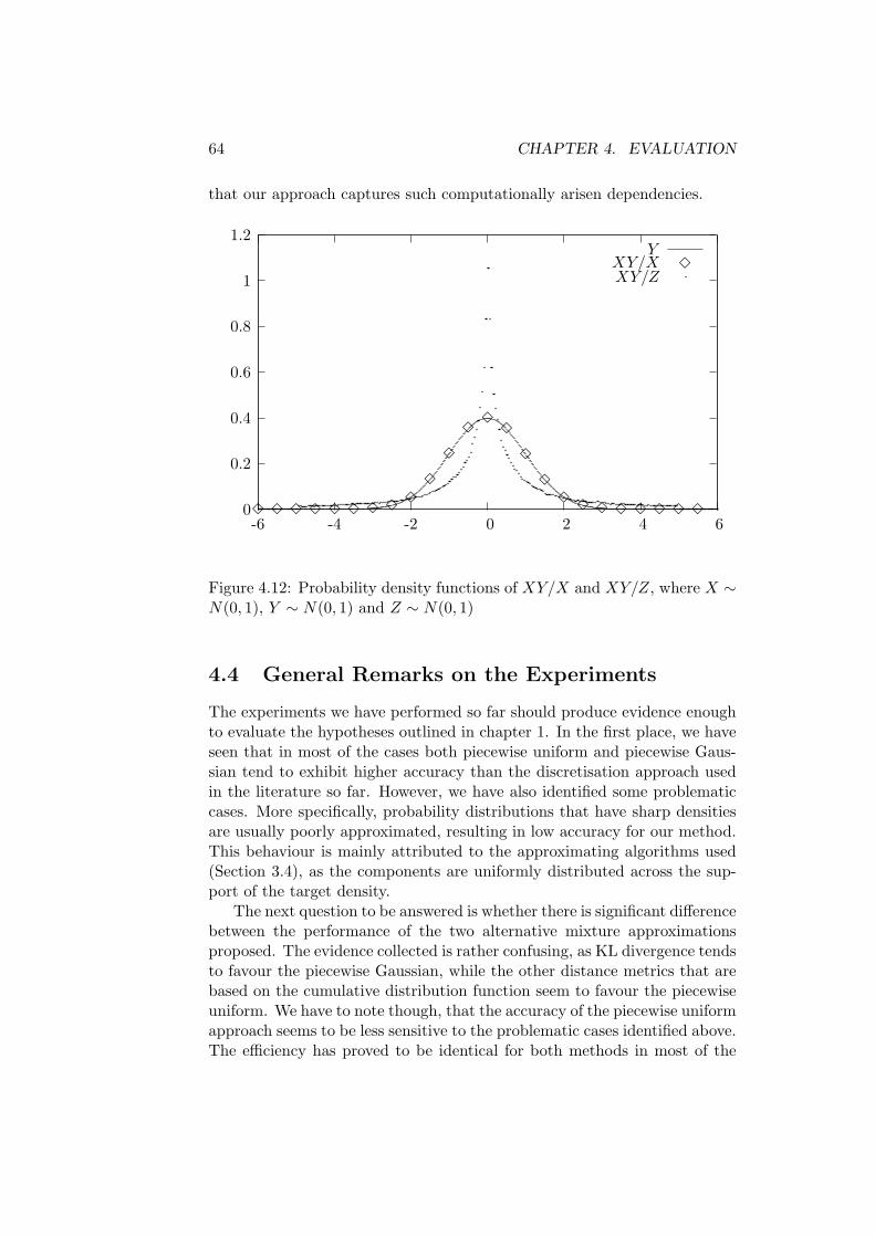
64 CHAPTER 4. EVALUATION
that our approach captures such computationally arisen dependencies.
0
0.2
0.4
0.6
0.8
1
1.2
-6 -4 -2 0 2 4 6
YXY/X
3 3 3 3 3 3 3 33
3
3
33
3
3
3
33 3 3 3 3 3 3
3XY/Z
Figure 4.12: Probability density functions of XY/X and XY/Z, where X ∼N(0, 1), Y ∼ N(0, 1) and Z ∼ N(0, 1)
4.4 General Remarks on the Experiments
The experiments we have performed so far should produce evidence enoughto evaluate the hypotheses outlined in chapter 1. In the first place, we haveseen that in most of the cases both piecewise uniform and piecewise Gaus-sian tend to exhibit higher accuracy than the discretisation approach usedin the literature so far. However, we have also identified some problematiccases. More specifically, probability distributions that have sharp densitiesare usually poorly approximated, resulting in low accuracy for our method.This behaviour is mainly attributed to the approximating algorithms used(Section 3.4), as the components are uniformly distributed across the sup-port of the target density.
The next question to be answered is whether there is significant differencebetween the performance of the two alternative mixture approximationsproposed. The evidence collected is rather confusing, as KL divergence tendsto favour the piecewise Gaussian, while the other distance metrics that arebased on the cumulative distribution function seem to favour the piecewiseuniform. We have to note though, that the accuracy of the piecewise uniformapproach seems to be less sensitive to the problematic cases identified above.The efficiency has proved to be identical for both methods in most of the
4.4. GENERAL REMARKS ON THE EXPERIMENTS 65
cases. However, we have to note that the running times are higher forpiecewise uniform, in the cases of binary sum and difference. This waspretty mush expected, since it is more expensive to determine the exactsum and difference of uniform components, as we have seen in Section 2.3.2.In any case, the use of more sophisticated approximating algorithms, whichis in the plans of future work, may change the entire picture.
Furthermore, the experiments on the dependency tracking verified thatour Monte Carlo implementation does actually cature the dependencies thatarise throughout the computations.

66 CHAPTER 4. EVALUATION
Chapter 5
Conclusion and Future Work
Summarising, the objective of this project was the development of a toolfor performing computations on random variables, both accurately and ef-ficiently. While the results for the computations discussed are well definedin terms of the probability theory, closed form expressions only exist for alimited number of distribution families and operations. Thus, we have in-troduced an approach that makes use of mixture model approximations inorder to perform computations on arbitrarily distributed random variables.In this way, a binary operation on random variables will be implemented asa series of operations on their approximating mixture components. We havedeveloped two alternative versions of this approach, using either mixturesof uniforms or mixtures of Gaussians.
Trying to estimate the performance of our system, we have outlined therelationship between efficiency and accuracy. The running times achievedusing 100 components are usually acceptable for real time computations.A further increase in the component number can actually improve the ac-curacy, but also has a significantly negative effect on the efficiency. Therunning times for binary operations seemed to increase in a quadratic man-ner, which is rather expected as the computational complexity with respectto the components is O(N2). So, the use of 100 approximating componentsis actually a trade-off between accuracy and efficiency.
The mixture model approach can be thought of as a generalisation of thediscretisation approach seen in previous works [29, 4, 33]. However, the cur-rently proposed method produces the resulting distributions by computingexactly the intermediate results of their components. So, we would expectto see an improvement in accuracy, in comparison with the discretisation-based methods. The experiments performed supply a good amount of evi-dence that seems to confirm this expectation. In fact, our system exhibitshigher accuracy in a number of cases, including the sum and the differenceof random variables, and some cases of the product and the ratio.
We have to note however that the accuracy achieved was not satisfac-
67
68 CHAPTER 5. CONCLUSION AND FUTURE WORK
tory in some cases. In particular, we have discovered that high probabilitydiscontinuous areas are poorly approximated by any of our approaches, espe-cially the piecewise Gaussian. This is actually because of the approximatingalgorithms we have used. In fact, the high efficiency of the approximationalgorithms chosen, came at the price of poor approximation accuracy forsharp densities. In both cases, we use a fixed number of components, wherethe neighbouring components have the same distance between each other.This entails that too many components are spent to approximate smoothareas of the target density, while sharper areas are approximated with lessthan adequate components. In terms of future work, it is certainly worthexperimenting on alternative algorithms that support variable number ofcomponents and variable distance between them.
Another important question that was supposed to be answered by theevaluation process, was whether any of our alternatives, uniform mixtureand Gaussian mixture, significantly outperforms the other. Well, the evi-dence is rather confusing regarding this question, as the accuracy seems tobe dependent on the type of operation and the densities of the input distri-butions. However, if we try more sophisticated approximators, the situationmay not be the same, so further investigation is needed.
We have also seen that series of computations on random variables arepossible to generate dependencies among them. The tracking of this kind ofdependencies was an issue discussed in this work as well. More specifically,we have suggested that the dependencies can be adequately captured by thegraph of flow of computations. However, this feature was not incorporatedto the main component that makes use of mixture models. Instead, wehave developed a Monte Carlo approach that takes advantage of that fea-ture, as a proof of concept prototype. After having performed a number ofexperiments, we have gathered evidence that confirm our suggestion. More-over, the dependency tracking Monte Carlo implementation can be used asa future point of reference.
All these findings discussed so far are rather encouraging for the furtherdevelopment of this project. The next task should be the improvementof the approximating process, as it seems to be responsible for the poorresults given for distributions with sharp densities. In this case, furtherexperimentation could be much more enlightening about the potential ofthe proposed method. Furthermore, since the use of computational graphsproved to adequately track the dependencies that are formed, it certainlymakes sense to be used in terms of the mixture model approximation.

Appendix A
Concrete DistributionClasses
The following classes represent the continuous distributions with known pa-rameters implemented so far. They can be components in a mixture model,so they implement the abstract MixtureComponent class. Along with theEmpiricalDistribution and the MixtureModel, they are the only distributionclasses visible to the users.
A.1 The Uniform Distribution Class
Parameters : endpoints a and b, where a < b
PDF : f(x) =
{1
b−a , x ∈ [a, b]0, otherwise
CDF : F (x) =
0, x < ax−ab−a , a ≤ x < b
1, b ≤ x
Constructor : Uniform(double a, double b)
A.2 The Gaussian Distribution Class
Parameters : mean µ and variance σ2, where σ2 > 0
PDF : f(x) = 1√2πσ2
e−(x−µ)2
2σ2
CDF : F (x) = 12 + 1
2erf(
x−µ√2σ2
)Constructor : Gaussian(double mean, double variance)
69

70 APPENDIX A. CONCRETE DISTRIBUTION CLASSES
The expressions exp(x) and erf(x) are computed using the correspondingfunctions of cmath library.
A.3 The Exponential Distribution Class
Parameters : rate λ, where λ > 0
PDF : f(x) = λe−λx
CDF : F (x) = 1− e−λx
Constructor : Exponential(double rate)
The expression exp(x) is computed using exp(double) function of cmathlibrary.
A.4 The Cauchy Distribution Class
Parameters : location x0 and scale γ, where γ > 0
PDF : f(x) = 1π
[γ
(x−x0)2+γ2
]CDF : F (x) = 1
πarctan(
x−x0γ
)+ 1
2
Constructor : Cauchy(double location, double scale)
The expression arctan(x) is computed using atan(double) function of cmathlibrary.
A.5 The ChiSquare Distribution Class
Parameters : degrees of freedom k, where k ∈ N∗
PDF : f(x) = (1/2)k/2
Γ(k/2) xk/2−1e−x/2
CDF : F (x) = γ(k/2,x/2)Γ(k/2)
Constructor : ChiSquare(double degrees_of_freedom)
The expressions Γ(x) and γ(s, x) are computed using the correspondingfunctions of boost library. Their definitions can be found in [1].

Appendix B
Code Examples of StochasticLibrary
B.1 Initialisation of Random Variables
#include <stochastic.h>
using namespace stochastic;
int main(){
// Any of the following is valid
RandomVariable a(new Gaussian(0, 1));
RandomVariable b = new Gaussian(0, 1);
Gaussian normal_distribution (0, 1);RandomVariable c = & normal_distribution;RandomVariable d(& normal_distribution );
return 0;}
71

72 APPENDIX B. CODE EXAMPLES OF STOCHASTIC LIBRARY
B.1.1 Initialisation Using a Dataset
#include <stochastic.h>
using namespace stochastic;
int main(){
// The distribution of the "raw" object is// directly defined by the dataset stored in// "dataDistribution" object.
EmpiricalDistribution dataDistribution ("data ");RandomVariable raw = & dataDistribution;
// The "refined" object is assigned an approximation// of the dataset ’s distribution.// The dataset may now be discarded.
PiecewiseGaussian approximation (& dataDistribution );RandomVariable refined = & approximation;
// It is reminded that PiecewiseUniform// and PiecewiseGaussian// are special cases of mixture models// that are used to approximate other distributions.
return 0;}
B.1.2 Initialisation Using a Mixture Model
#include <stochastic.h>#include <vector >
using namespace stochastic;
int main(){
std:: vector <MixtureComponent *> c; // componentsstd:: vector <double > w; // weights
c.push_back(new Gaussian(0, 1));c.push_back(new Gaussian(3, 2));w.push_back (2);w.push_back (1);// the weights will be normalised

B.2. SWITCH AMONG METHODS OF COMPUTATION 73
// Tass the components and the weights defined// to the MixtureModel constructor.
// Then , pass the MixtureModel created// to a RandomVariable
RandomVariable mixture_model = new MixtureModel(c, w);
return 0;}
B.2 Switch among Methods of Computation
#include <stochastic.h>
using namespace stochastic;
int main(){
RandomVariable a = new Gaussian(0, 1);RandomVariable b = new Gaussian(3, 2);
// Each time , the exression "a + b"// will be computed in a different way
// Monte Carlo with 1000 samplesRandomVariable :: setMonteCarlo (1000);a + b;
// Piecewise uniform with 100 componentsRandomVariable :: setPiecewiseUniform (100);a + b;
// Piecewise Gaussian with 100 componentsRandomVariable :: setPiecewiseGaussian (100);a + b;
return 0;}

74 APPENDIX B. CODE EXAMPLES OF STOCHASTIC LIBRARY

Bibliography
[1] Milton Abramowitz and Irene A. Stegun. Handbook of MathematicalFunctions with Formulas, Graphs, and Mathematical Tables. Dover,New York, ninth dover printing, tenth gpo printing edition, 1964.
[2] D. Alspach and H. Sorenson. Nonlinear bayesian estimation usinggaussian sum approximations. IEEE Trans. on Automatic Control,(17):438–448, 1972.
[3] Leo A. Aroian. The probability function of the product of two nor-mally distributed variables. In The Annals of Mathematical Statistics,volume 18, pages 265–271, 1947.
[4] D. Berleant and C. Goodman-Strauss. Bounding the results of arith-metic operations on random variables of unknown dependency usingintervals. In Reliable Computing, volume 4, pages 147–165, May 1998.
[5] D. Berleant and J. Zhang. Arithmetic on random variables: Squeezingthe envelopes with new joint distribution constraints. In 4th Interna-tional Symposium on Imprecise Probabilities and Their Applications,2005.
[6] Christopher M. Bishop. Pattern Recognition and Machine Learning.Springer Science+Business Media, 233 Spring Street, New York, NY10013, USA, first edition, 2006.
[7] R.L. Burden and J.D. Faires. Numerical Analysis. Brooks/Cole, seventhedition, 2000.
[8] E.v. Collani and F. Killmann. A note on the convolution of uniformand related distributions and their use in quality control. In EconomicQuality Control, volume 16, pages 17–41, 2001.
[9] A.G. Colombo and R.J. Jaarsma. A powerful numerical method tocombine random variables. In IEEE Transactions on Reliability, pages126–129, June 1980.
[10] C.C. Craig. On the frequency function of xy. In The Annals of Math-ematical Statistics, volume 7, pages 1–15, 1936.
75

76 BIBLIOGRAPHY
[11] J.H. Curtiss. On the distribution of the quotient of two chance variables.In The Annals of Mathematical Statistics, volume 12, pages 409–421.Institute of Mathematical Statistics, December 1941.
[12] L. Xie D. Berleant and J. Zhang. Statool: A tool for distribution enve-lope determination (denv), an interval-based algorithm for arithmeticon random variables. In Reliable Computing, volume 9, pages 91–108,April 2003.
[13] A. DasGupta. Asymptotic Theory of Statistics and Probability. SpringerTexts in Statistics, first edition, 2008.
[14] A. P. Dempster, N. M. Laird, and D. B. Rubin. Maximum likelihoodfrom incomplete data via the em algorithm. Journal of the Royal Sta-tistical Society. Series B (Methodological), 39(1):1–38, 1977.
[15] Luc Devroye. Non-Uniform Random Variate Generation. Springer,1986.
[16] Benjamin Epstein. Some applications of the mellin transform in statis-tics. In The Annals of Mathematical Statistics, volume 19, pages 370–379, Sep 1948.
[17] William Feller. An Introduction to Probability Theory and Its Applica-tions, Volume 1. Wiley, January 1968.
[18] D. Freedman and P. Diaconis. On the histogram as a density estimator:L2 theory. 57(4):453–476, December 1981.
[19] R. Fruhwirth. A gaussian-mixture approximation of the betheheitlermodel of electron energy loss by bremsstrahlung. In Computer PhysicsCommunications, volume 154, pages 131–142, 2003.
[20] J. Galambos. Advanced Probability Theory. CRC Press, second edition,1995.
[21] Noah D. Goodman, Vikash K. Mansinghka, Daniel Roy, KeithBonawitz, and Joshua B. Tenenbaum. Church: a language for gen-erative models. In Uncertainty in Artificial Intelligence, 2008.
[22] Charles M. Grinstead and James L. Snell. Introduction to Probability.AMS Bookstore, second edition, 1997.
[23] J.C. Hayya and W.L. Ferrara. On normal approximations of the fre-quency functions of standard forms where the main variables are nor-mally distributed. In Management Science, volume 19, pages 173–186,1972.
BIBLIOGRAPHY 77
[24] J.R. Hershey and P.A. Olsen. Approximating the kullback leibler diver-gence between gaussian mixture models. In IEEE International Confer-ence on Acoustics, Speech and Signal Processing, 2007. ICASSP 2007.,volume 4, pages IV–317–IV–320, 2007.
[25] D.V. Hinkley. On the ratio of two correlated normal random variables.In Biometrika, volume 56, pages 635–639, 1969.
[26] S. Ferson H.M. Regan and D. Berleant. Equivalence of methods for un-certainty propagation of real-valued random variables. In InternationalJournal of Approximate Reasoning, volume 36, pages 1–30, April 2004.
[27] Hwei P. Hsu. Probability, Random Variables, and Random Processes.McGraw-Hill, 1996.
[28] S. Chakraborti J.D. Gibbons. Nonparametric Statistical Inference. Mar-cel Dekker Inc., 270 Madison Avenue, New York, NY 10016, USA,fourth edition, 2003.
[29] S. Kaplan. On the method of discrete probability distributions in riskand reliability calculations—application to seismic risk assessment. InRisk Analysis, volume 1, pages 189–196, August 1981.
[30] R.B. Kearfott and V. Kreinovich. Applications of interval computations.Kluwer Academic Publishers, first edition, 1995.
[31] Solomon Kullback and Richard A. Leibler. On information and suffi-ciency. The Annals of Mathematical Statistics, 22(1):79–86, 1951.
[32] Laha and J. Roy Chakravarti. Handbook of Methods of Applied StatisticsVolume I. John Wiley and Sons, 1967.
[33] W. Li and J.M. Hyman. Computer arithmetic for probability distribu-tion variables. In Reliability Engineering and System Safety, volume 85,pages 191–209, April 2004.
[34] Z.A. Lomnicki. On the distribution of products of random variables.29(3):513–524, 1967.
[35] David J.C. MacKay. Information Theory, Inference, and Learning Al-gorithms. Cambridge University Press, first edition, 2003.
[36] N. Metropolis and S. Ulam. The monte carlo method. 44(247):335341,September 1949.
[37] R.B. Nelsen M.J. Frank and B. Schweizer. Best-possible bounds for thedistribution of a sum—a problem of kolmogorov. In Probability Theoryand Related Fields, volume 74, pages 199–211, June 1987.

78 BIBLIOGRAPHY
[38] R.E. Moore. Risk analysis without monte carlo methods. pages 1–48,1984.
[39] R.B. Nelsen. An Introduction to Copulas (Springer Series in Statistics).Springer-Verlag New York, Inc., Secaucus, NJ, USA, 2006.
[40] The Distribution of Products of Independent Random Variables. M. d.springer and w. e. thompson. In SIAM Journal on Applied Mathematics,volume 14, pages 511–526, May 1966.
[41] Athanasios Papoulis. Probability, Random Variables and StochasticProcesses. McGraw-Hill Companies, February 1991.
[42] E. Parzen. On the estimation of a probability density function and themode. In Annals of Mathematical Statistics, volume 33, pages 1065–1076, September 1962.
[43] E. Parzen. Nonparametric statistical data modeling. In Journal ofthe American Statistical Association, volume 74, pages 105–121, March1979.
[44] V.K. Rohatgi. An Introduction to Probability Theory MathematicalStatistics. Wiley, New York, 1976.
[45] R.Y. Rubinstein and D.P. Kroese. Simulation and the Monte CarloMethod. John Wiley & Sons, Inc., second edition, 2008.
[46] Marvin K. Simon. Probability Distributions Involving Gaussian RandomVariables: A Handbook for Engineers, Scientists and Mathematicians.Springer-Verlag New York, Inc., Secaucus, NJ, USA, 2006.
[47] M.D. Springer. The Algebra of Random Variables. Wiley, first edition,1979.
[48] K. Thulasiraman and M. N. S. Swamy. Graphs: Theory and Algorithms.John Wiley and Son, 1992.
[49] J. von Neumann. Various techniques used in connection with randomdigits. monte carlo methods. In National Bureau of Standards, vol-ume 12, pages 36–38, 1951.
[50] L. Wasserman. All of Statistics: A Concise Course in Statistical Infer-ence. Springer Texts in Statistics, 2005.
[51] R. C. Williamson and T. Downs. Probabilistic arithmetic. i. numericalmethods for calculating convolutions and dependency bounds. Int. J.Approx. Reasoning, 4(2):89–158, 1990.

BIBLIOGRAPHY 79
[52] J. Wolfowitz. Additive partition functions and a class of statisticalhypotheses. In Annals of Mathematical Statistics, volume 13, pages247–279, September 1942.


