Probability Distributions - Chapter 2 - Grandinetti · 2017-08-25 · Probability Distributions...

Probability DistributionsChapter 2

P. J. Grandinetti

Chem. 4300

Aug. 25, 2017

P. J. Grandinetti (Chem. 4300) Probability Distributions Aug. 25, 2017 1 / 27

Temperature of solution in “constant temperature” bath

Measurement Number

31.331.231.131.030.930.830.7

Tem

pera

ture

(°C

)

What do you report for the solutiontemperature?

N = 128

30.8 30.9 31.0 31.1 31.2 31.3

8

6

4

2

0

Cou

nt

Temperature (°C)

histogram,aka the sample distribution

the mean temperature (31.1 ◦C)

histogram of all measured values


Sample and parent distribution

We assume that our histogram of measured values is governed by anunderlying probability distribution called the parent distribution.

parent distribution

In the limit of an infinite number of measurements our histogram orsample distribution becomes the parent distribution.


Sample and parent distributionHistograms (sample distributions) constructed from the same parent distribution

N = 4096

30.8 30.9 31.0 31.2 31.3 31.4

0.4

0.3

0.2

0.1

0.0

N = 128

30.8 30.9 31.0 31.1 31.2 31.3 31.4

0.4

0.3

0.2

0.1

0.0

31.1

Prob

abili

tyD

ensi

ty

N = 1024

30.8 30.9 31.0 31.1 31.2 31.3 31.4

0.4

0.3

0.2

0.1

0.0

Prob

abili

tyD

ensi

tyPr

obab

ility

Den

sity

N = 128

30.8 30.9 31.0 31.1 31.2 31.3 31.4

0.4

0.3

0.2

0.1

0.0

N = 1024

30.8 30.9 31.0 31.1 31.2 31.3 31.4

0.4

0.3

0.2

0.1

0.0

N = 4096

30.8 30.9 31.0 31.2 31.3 31.4

0.4

0.3

0.2

0.1

0.031.1

A B

N = 128

30.8 30.9 31.0 31.1 31.2 31.3 31.4

0.4

0.3

0.2

0.1

0.0

N = 1024

30.8 30.9 31.0 31.1 31.2 31.3 31.4

0.4

0.3

0.2

0.1

0.0

N = 4096

30.8 30.9 31.0 31.2 31.3 31.4

0.4

0.3

0.2

0.1

0.031.1

C

Temperature/°C Temperature/°C Temperature/°C




Probability density

Our main objective in making a measurement is to learn the underlyingparent distribution, p(x), that predicts the spread in the measured values.

The parent distribution, p(x), is also called a probability density. A parentdistribution is always normalized so the area under the distribution is unity,∫

all xp(x) dx = 1.


Confidence Limits

The probability that a measured value lies between x− and x+ can becalculated from the parent distribution according to

P(x−, x+) =

∫ x+

x−

p(x) dx .

The integral limits x− and x+ are called the confidence limits associatedwith a given probability P(x−, x+).


Moments of a distribution

When you report confidence limits you lose information concerning theshape of the parent distribution.

There are a few parameters that by convention are often used to describethe parent distribution in part, or sometimes completely.

mean : the first moment about the origin

variance : the second moment about the mean

skewness : the third moment about the mean

kurtosis : the fourth moment about the mean


The mean

The Mean describes the average value of the distribution. Given theparent distribution, p(x), the mean is calculated according to

µ =

∫all x

x p(x) dx .

From a series of measurements the mean is given by

µ = limN→∞

1

N

∑i

xi ,

where N corresponds to the number of measurements xi .

Practically, we cannot make an infinite measurements so the experimentalmean, x , is defined as

x =1

N

∑i

xi .


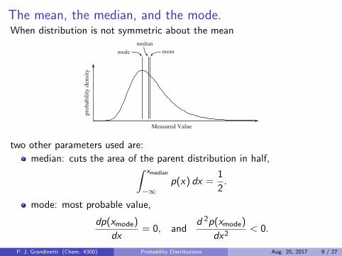
The mean, the median, and the mode.When distribution is not symmetric about the mean

modemedian

mean

Measured Value

prob

abili

ty d

ensi

ty

two other parameters used are:

median: cuts the area of the parent distribution in half,∫ xmedian

−∞p(x) dx =

1

2.

mode: most probable value,

dp(xmode)

dx= 0, and

d 2p(xmode)

dx2< 0.


The Variance.Variance characterizes the width of the distribution and is given by

σ2 =

∫all x

(x − µ)2p(x)dx .

From a series of measurements the variance is obtained through:

σ2 = limN→∞

1

N

N∑i

(xi − µ)2.

The experimental variance is defined as:

s2 =1

N − 1

N∑i

(xi − x)2,

where s2 is the variance of the experimental parent distribution.σ and s are the standard deviation of the parent distribution andexperimental parent distribution, respectively.


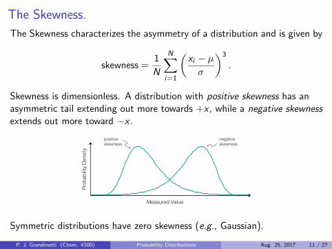
The Skewness.

The Skewness characterizes the asymmetry of a distribution and is given by

skewness =1

N

N∑i=1

(xi − µ

σ

)3

.

Skewness is dimensionless. A distribution with positive skewness has anasymmetric tail extending out more towards +x , while a negative skewnessextends out more toward −x .

positiveskewness

negativeskewness

Measured Value

Prob

abilit

y D

ensi

ty

Symmetric distributions have zero skewness (e.g., Gaussian).


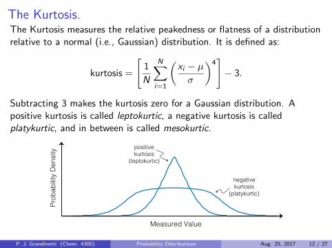
The Kurtosis.The Kurtosis measures the relative peakedness or flatness of a distributionrelative to a normal (i.e., Gaussian) distribution. It is defined as:

kurtosis =

[1

N

N∑i=1

(xi − µ

σ

)4]− 3.

Subtracting 3 makes the kurtosis zero for a Gaussian distribution. Apositive kurtosis is called leptokurtic, a negative kurtosis is calledplatykurtic, and in between is called mesokurtic.

negativekurtosis

(platykurtic)

positivekurtosis

(leptokurtic)

Measured Value

Prob

abilit

y D

ensi

ty


Probability

Probability =Number of outcomes that are successful (winning)

Total number of outcomes (winning and losing)

The difficulty lies in counting. In order to count the number of outcomeswe appeal to combinatorics.


Permutations

Definition

Permutation An arrangement of outcomes in which the order is important.

Example

Consider a club with 5 members, Joe, Kathy, Sally, Bob, and Pat. In howmany ways can we elect a president and a secretary?

One solution

One solution is to make a tree, such as the one below:

Joe

Joe, KathyJoe, SallyJoe, BobJoe, Pat

Kathy

Kathy, JoeKathy, SallyKathy, BobKathy, Pat

Pat

Pat, JoePat, KathyPat, SallyPat, Bob

Sally

Sally, JoeSally, KathySally, BobSally, Pat

Bob

Bob, JoeBob, KathyBob, SallyBob, Pat

Using such a tree diagram we can count that there are a total of 20possible ways to elect a president and a secretary in a club with 5members.

Another solution

Think of two boxes, one for president, and one for secretary. If you pickthe president first and secretary second then you’ll have five choices forpresident 5 president, and four choices for secretary 4 secretary. The totalnumber of ways is the product of the two numbers

5 president · 4 secretary = 20.


Permutations

Example

What if we wanted to elect a president, secretary, and treasurer?

Solution

In this case a tree would be a lot of work. Using the boxes approach wewould have 5 · 4 · 3 = 60 possibilities.

The number of ways r objects can be selected from n objects is

nPr = n · (n − 1) · (n − 2) · · · (n − r + 1),

or more generally written as

nPr =n!

(n − r)!.


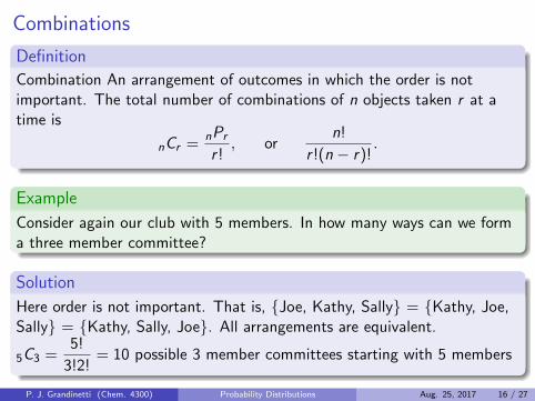
Combinations

Definition

Combination An arrangement of outcomes in which the order is notimportant. The total number of combinations of n objects taken r at atime is

nCr =nPr

r !, or

n!

r !(n − r)!.

Example

Consider again our club with 5 members. In how many ways can we forma three member committee?

Solution

Here order is not important. That is, {Joe, Kathy, Sally} = {Kathy, Joe,Sally} = {Kathy, Sally, Joe}. All arrangements are equivalent.

5C3 =5!

3!2!= 10 possible 3 member committees starting with 5 members


Combinations

Definition

Combination An arrangement of outcomes in which the order is notimportant. The total number of combinations of n objects taken r at atime is

nCr =nPr

r !, or

n!

r !(n − r)!.

nCr is called the binomial coefficient, and is also often written as

(nr

).(

nr

)=

n!

r !(n − r)!


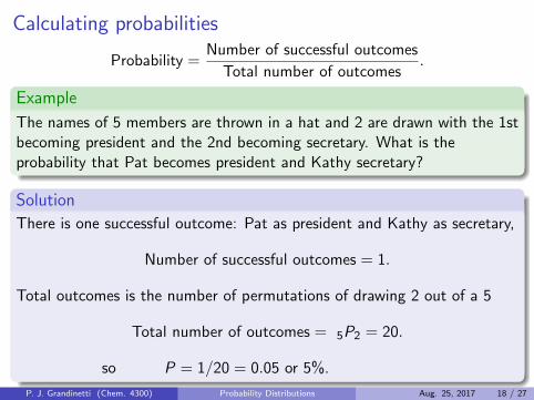
Calculating probabilities

Probability =Number of successful outcomes

Total number of outcomes.

Example

The names of 5 members are thrown in a hat and 2 are drawn with the 1stbecoming president and the 2nd becoming secretary. What is theprobability that Pat becomes president and Kathy secretary?

Solution

There is one successful outcome: Pat as president and Kathy as secretary,

Number of successful outcomes = 1.

Total outcomes is the number of permutations of drawing 2 out of a 5

Total number of outcomes = 5P2 = 20.

so P = 1/20 = 0.05 or 5%.


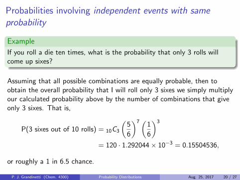
Probabilities involving independent events with sameprobability

Example

If you roll a die ten times, what is the probability that only 3 rolls willcome up sixes?

What is the probability of rolling only 3 sixes? e.g., one way it couldhappen is

X ,X , 6,X ,X ,X , 6, 6,X ,X

where X is a roll that was not 6.The probability of this particular sequence of independent events is

p =5

6· 56· 16· 56· 56· 56· 16· 16· 56· 56=

(5

6

)7(1

6

)3

= 1.292044× 10−3

How many ways can we roll only 3 sixes?X , X , 6 , X , X , X , 6 , 6 , X , XX , X , X , 6 , X , X , 6 , 6 , X , XX , X , X , 6 , X , 6 , X , 6 , X , X

...

The total number of possibilities (i.e., combinations) is 10C3 or

(103

).


Probabilities involving independent events with sameprobability

Example

If you roll a die ten times, what is the probability that only 3 rolls willcome up sixes?

Assuming that all possible combinations are equally probable, then toobtain the overall probability that I will roll only 3 sixes we simply multiplyour calculated probability above by the number of combinations that giveonly 3 sixes. That is,

P(3 sixes out of 10 rolls) = 10C3

(5

6

)7(1

6

)3

= 120 · 1.292044× 10−3 = 0.15504536,

or roughly a 1 in 6.5 chance.


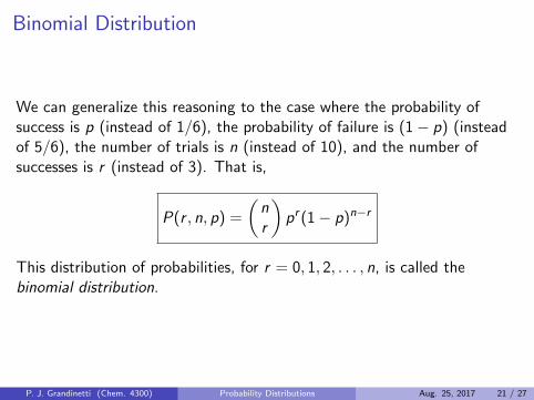
Binomial Distribution

We can generalize this reasoning to the case where the probability ofsuccess is p (instead of 1/6), the probability of failure is (1− p) (insteadof 5/6), the number of trials is n (instead of 10), and the number ofsuccesses is r (instead of 3). That is,

P(r , n, p) =

(nr

)pr (1− p)n−r

This distribution of probabilities, for r = 0, 1, 2, . . . , n, is called thebinomial distribution.



r Prob.012345678910

9.77 X 10- 4

9.77 X 10- 3

0.1170.2050.2460.2050.1170.044

9.77 X 10- 49.77 X 10- 30.044

0 2 4 6 8 100.00

0.05

0.10

0.15

0.20

0.25

Prob

abili

ty

r

μ = 5

σ = 1.58

(a)

0 2 4 6 8 100.00

0.05

0.10

0.15

0.20

0.25

0.30

0.35

r

μ = 1.67

σ = 1.18

Prob

abili

ty

r Prob.012345678910

0.1620.323

0.000250.0020.0130.0540.1550.291

1.65 X 10-80.00000080.00002

(b)

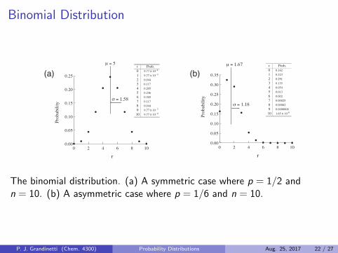
The binomial distribution. (a) A symmetric case where p = 1/2 andn = 10. (b) A asymmetric case where p = 1/6 and n = 10.



The mean and variance of a discrete distribution is given by

µr =rmax∑r=0

rP(r), and σ2r =

rmax∑r=0

(r − µr )2P(r).

The mean of the binomial distribution to be

µ =n∑

r=0

r

(nr

)pr (1− p)n−r = np,

and the variance of the binomial distribution to be

σ2 =n∑

r=0

[(r − µ)2

(nr

)pr (1− p)n−r

]= np(1− p).


Poisson DistributionIn the limit that n → ∞ and p → 0 such that np → a finite number thebinomial distribution becomes the Poisson Distribution given by

PPoisson(r , n, p) =(np)r

r !e−np.

This distribution often describes the parent distribution for observingindependent random events that are occurring at a constant rate, such asphoton counting experiments.The mean of the Poisson distribution is

µ =∞∑r=0

[r(np)r

r !e−np

]= np.

and the variance of the Poisson distribution is

σ2 =∞∑r=0

[(r − np)2

(np)r

r !e−np

]= np.


Gaussian DistributionIn the limit of large n when p is not close to zero we can use the Gaussiandistribution as an approximation for the binomial. That is,

PGaussian(r , n, p) =1√

2πnp(1− p)exp

{−1

2

(r − np)2

np(1− p)

}.

The mean of the Gaussian distribution is

µ =∞∑r=0

[r√

2πnp(1− p)exp

{−1

2

(r − np)2

np(1− p)

}]= np.

and the variance of the Gaussian distribution is

σ2 =∞∑r=0

[(r − np)2√2πnp(1− p)

exp

{−1

2

(r − np)2

np(1− p)

}]= np(1− p).

Making the substitutions for µ = np and σ2 = np(1− p) we can rewritethe Gaussian distribution


Gaussian Distribution in the continuous variable limit

Making the substitutions for µ = np and σ2 = np(1− p) we can rewritethe Gaussian distribution in the form

PGaussian(r , µ;σ) =1

σ√2π

exp

{−1

2

(r − µ

σ

)2}.

Replacing the integer r with a continuous parameter x and get

pGaussian(x , µ;σ) =1

σ√2π

exp

{−1

2

(x − µ

σ

)2}.


Gaussian Distribution

-5σ -4σ -3σ -2σ -σ 0 σ 2σ 3σ 4σ 5σx − μ

Area between ±zσ = ±0.67σ is 50% of total area

+0.67σ -0.67σ

+1.96σ -1.96σ

0.40/σ

0.35/σ

0.30/σ

0.25/σ

0.20/σ

0.15/σ

0.10/σ

0.05/σ0.00/σ

prob

abili

ty d

ensi

ty

-5σ -4σ -3σ -2σ -σ 0 σ 2σ 3σ 4σ 5σx − μ

Area between ±zσ = ±1.96 σ is 95% of total area

0.40/σ

0.35/σ

0.30/σ

0.25/σ

0.20/σ

0.15/σ

0.10/σ

0.05/σ0.00/σ

prob

abili

ty d

ensi

ty


Date post:	30-Jun-2018
Category:	Documents
Upload:	lekhanh
View:	219 times
Download:	0 times

Probability Distributions - Chapter 2 - Grandinetti · 2017-08-25 · Probability Distributions...

Documents