Probability Foundations

Rudolf Kruse, Pascal Held Bayesian Networks 35

Probability Foundations

Reminder: Probability Theory


Goal: Make statements and/or predictions aboutresults of physical processes.

Even processes that seem to be simple at first sightmay reveal considerable difficulties when trying to predict.

Describing real-world physical processes always callsfor a simplifying mathematical model.

Although everybody will have some intuitive notion aboutprobability, we have to formally define the underlyingmathematical structure.

Randomness or chance enters as the incapability of preciselymodelling a process or the inability of measuring the initial conditions.

Example : Predicting the trajectory of a billard ball over more than 9 banksrequires more detailed measurement of the initial conditions (ball location,applied momentum etc.) than physically possible according to Heisenberg’suncertainty principle.

Formal Approach on the Model Side


We conduct an experiment that has a set Ω of possible outcomes.E. g.:

Rolling a die (Ω = 1, 2, 3, 4, 5, 6) Arrivals of phone calls (Ω = N0)

Bread roll weights (Ω = R+)

Such an outcome is called an elementary event.

All possible elementary events are called the frame of discernment Ω(or sometimes universe of discourse).

The set representation stresses the following facts:

All possible outcomes are covered by the elements of Ω.(collectively exhaustive).

Every possible outcome is represented by exactly one element of Ω.(mutual disjoint).

Events


Often, we are interested in higher-level events(e. g. casting an odd number, arrival of at least 5 phone calls orpurchasing a bread roll heavier than 80 grams)

Any subset A ⊆ Ω is called an event which occurs, if the outcome ω0 ∈ Ω ofthe random experiment lies in A:

Event A ⊆ Ω occurs ⇔∨

ω∈A(ω = ω0) = true ⇔ ω0 ∈ A

Since events are sets, we can define for two events A and B:

A ∪ B occurs if A or B occurs; A ∩ B occurs if A and B occurs.

A occurs if A does not occur (i. e., if Ω\A occurs).

A and B are mutually exclusive, iff A ∩ B = ∅.

Event Algebra


A family of sets E = E1, . . . , En is called an event algebra,if the following conditions hold:

The certain event Ω lies in E . If E ∈ E , then E = Ω\E ∈ E . If E1 and E2 lie in E , then E1 ∪ E2 ∈ E and E1 ∩ E2 ∈ E .

If Ω is uncountable, we require the additional property:

For a series of events Ei ∈ E , i ∈ N, the events∞⋃

i=1

Ei and∞⋂

i=1

Ei are also in E .E is then called a σ-algebra.

Side remarks:

Smallest event algebra: E = ∅,ΩLargest event algebra (for finite or countable Ω): E = 2Ω = A ⊆ Ω | true

Probability Function


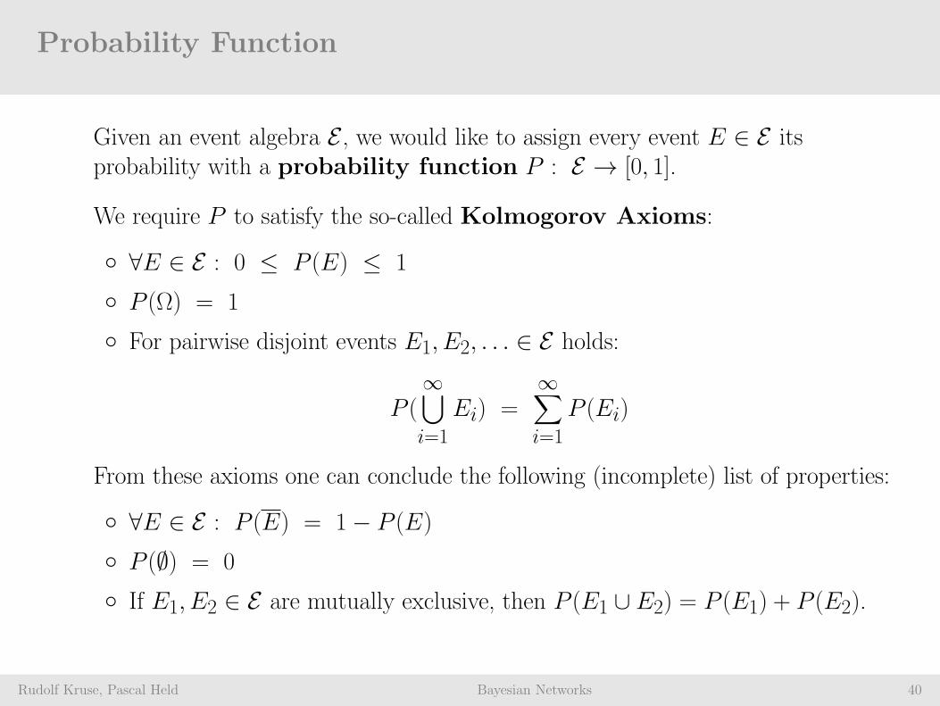
Given an event algebra E , we would like to assign every event E ∈ E itsprobability with a probability function P : E → [0, 1].

We require P to satisfy the so-called Kolmogorov Axioms:

∀E ∈ E : 0 ≤ P (E) ≤ 1

P (Ω) = 1

For pairwise disjoint events E1, E2, . . . ∈ E holds:

P (∞⋃

i=1

Ei) =∞∑

i=1

P (Ei)

From these axioms one can conclude the following (incomplete) list of properties:

∀E ∈ E : P (E) = 1− P (E) P (∅) = 0

If E1, E2 ∈ E are mutually exclusive, then P (E1 ∪ E2) = P (E1) + P (E2).

Elementary Probabilities and Densities


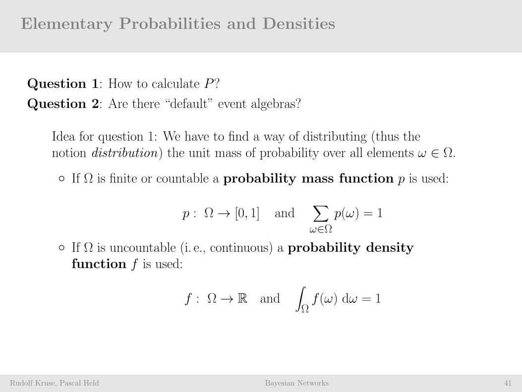
Question 1: How to calculate P ?

Question 2: Are there “default” event algebras?

Idea for question 1: We have to find a way of distributing (thus thenotion distribution) the unit mass of probability over all elements ω ∈ Ω.

If Ω is finite or countable a probability mass function p is used:

p : Ω→ [0, 1] and∑

ω∈Ωp(ω) = 1

If Ω is uncountable (i. e., continuous) a probability densityfunction f is used:

f : Ω→ R and∫

Ωf (ω) dω = 1

“Default” Event Algebras


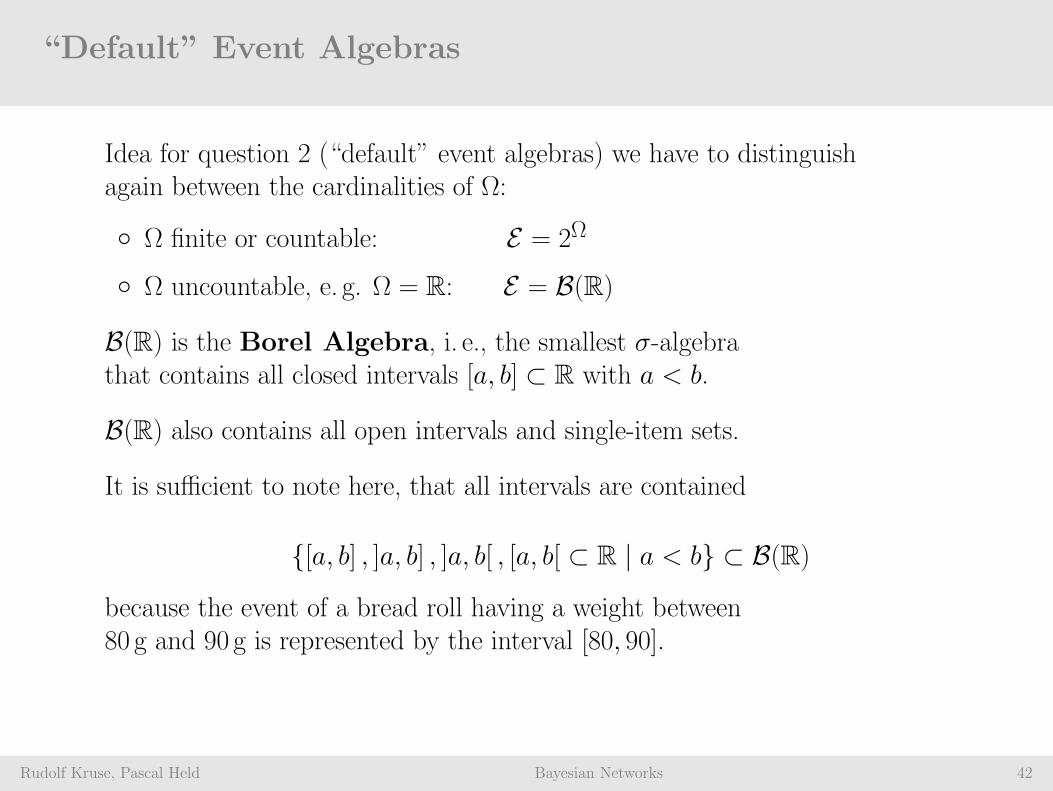
Idea for question 2 (“default” event algebras) we have to distinguishagain between the cardinalities of Ω:

Ω finite or countable: E = 2Ω

Ω uncountable, e. g. Ω = R: E = B(R)

B(R) is the Borel Algebra, i. e., the smallest σ-algebrathat contains all closed intervals [a, b] ⊂ R with a < b.

B(R) also contains all open intervals and single-item sets.

It is sufficient to note here, that all intervals are contained

[a, b] , ]a, b] , ]a, b[ , [a, b[ ⊂ R | a < b ⊂ B(R)because the event of a bread roll having a weight between80 g and 90 g is represented by the interval [80, 90].

Example: Rolling a Die


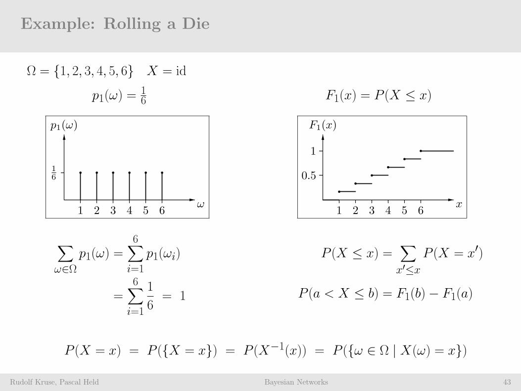
Ω = 1, 2, 3, 4, 5, 6 X = id

p1(ω) =16 F1(x) = P (X ≤ x)

1 2 3 4 5 6

1

6

ω

p1(ω)

1 2 3 4 5 6

1

0.5

x

F1(x)

∑

ω∈Ωp1(ω) =

6∑

i=1

p1(ωi)

=6∑

i=1

1

6= 1

P (X ≤ x) =∑

x′≤xP (X = x′)

P (a < X ≤ b) = F1(b)− F1(a)

P (X = x) = P (X = x) = P (X−1(x)) = P (ω ∈ Ω | X(ω) = x)


Basics of Applied Probability Theory

Why (Kolmogorov) Axioms?


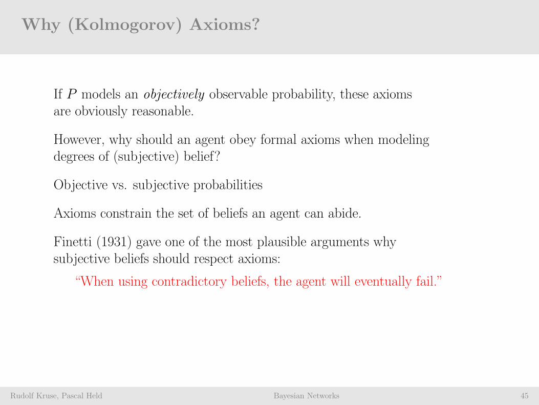
If P models an objectively observable probability, these axiomsare obviously reasonable.

However, why should an agent obey formal axioms when modelingdegrees of (subjective) belief?

Objective vs. subjective probabilities

Axioms constrain the set of beliefs an agent can abide.

Finetti (1931) gave one of the most plausible arguments whysubjective beliefs should respect axioms:

“When using contradictory beliefs, the agent will eventually fail.”

Unconditional Probabilities


P (A) designates the unconditioned or a priori probabilitythat A ⊆ Ω occurs if no other additional information is present.

For example:

P (cavity) = 0.1

Note: Here, cavity is a proposition.

A formally different way to state the same would be viaa binary random variable Cavity:

P (Cavity = true) = 0.1

A priori probabilities are derived from statistical surveys or general rules.

Unconditional Probabilities


In general a random variable can assume more than two values:

P ( Weather = sunny ) = 0.7

P ( Weather = rainy ) = 0.2

P ( Weather = cloudy) = 0.02

P ( Weather = snowy ) = 0.08

P (Headache = true ) = 0.1

P (X) designates the vector of probabilities for the(ordered) domain of the random variable X :

P (Weather) = 〈0.7, 0.2, 0.02, 0.08〉P (Headache) = 〈0.1, 0.9〉

Both vectors define the respective probability distributionsof the two random variables.

Conditional Probabilities


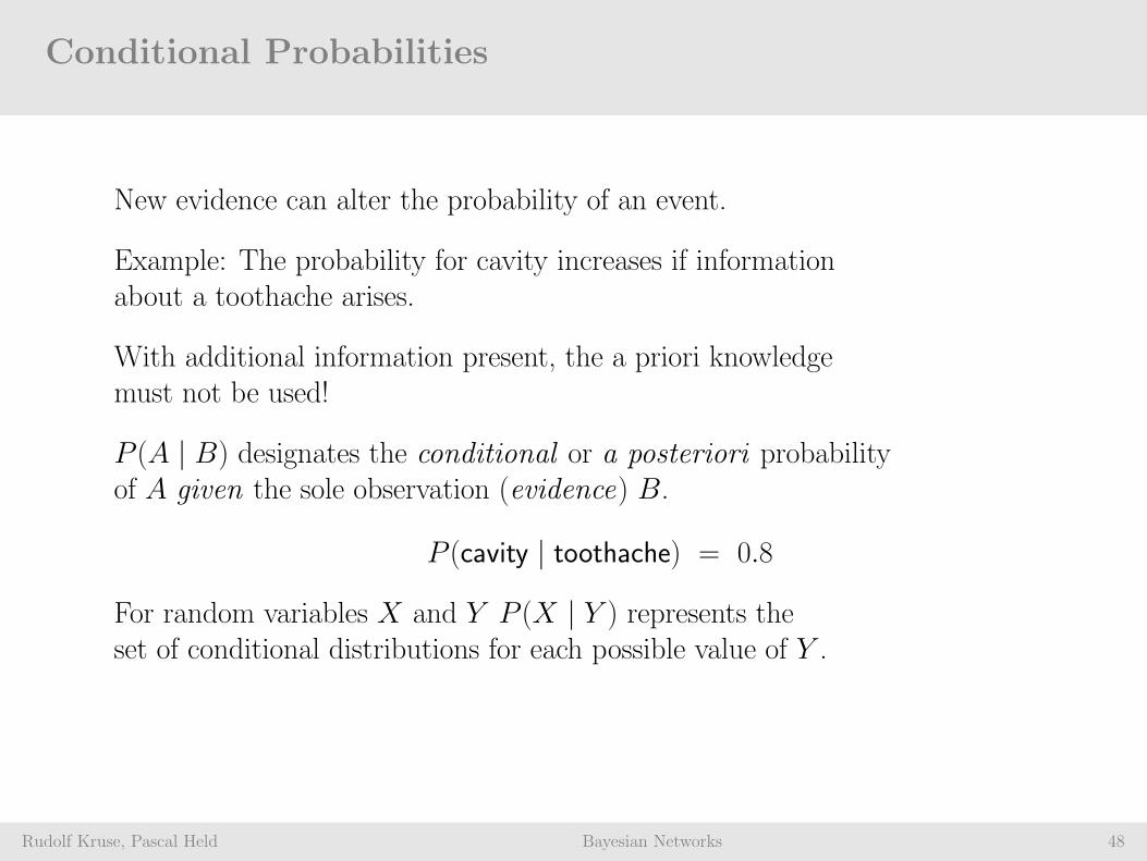
New evidence can alter the probability of an event.

Example: The probability for cavity increases if informationabout a toothache arises.

With additional information present, the a priori knowledgemust not be used!

P (A | B) designates the conditional or a posteriori probabilityof A given the sole observation (evidence) B.

P (cavity | toothache) = 0.8

For random variables X and Y P (X | Y ) represents theset of conditional distributions for each possible value of Y .



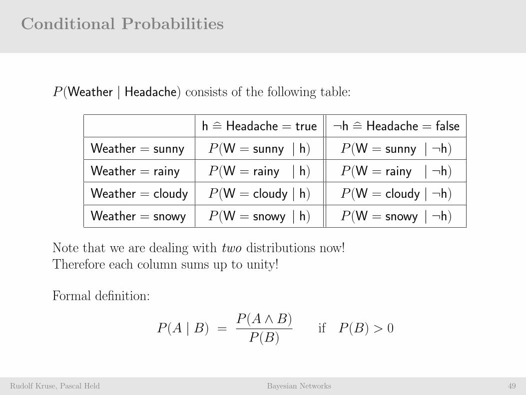
P (Weather | Headache) consists of the following table:

h = Headache = true ¬h = Headache = false

Weather = sunny P (W = sunny | h) P (W = sunny | ¬h)Weather = rainy P (W = rainy | h) P (W = rainy | ¬h)Weather = cloudy P (W = cloudy | h) P (W = cloudy | ¬h)Weather = snowy P (W = snowy | h) P (W = snowy | ¬h)

Note that we are dealing with two distributions now!Therefore each column sums up to unity!

Formal definition:

P (A | B) =P (A ∧ B)

P (B)if P (B) > 0



P (A | B) =P (A ∧ B)

P (B)

Product Rule: P (A ∧B) = P (A | B) · P (B)

Also: P (A ∧ B) = P (B | A) · P (A)

A and B are independent iff

P (A | B) = P (A) and P (B | A) = P (B)

Equivalently, iff the following equation holds true:

P (A ∧ B) = P (A) · P (B)

Interpretation of Conditional Probabilities


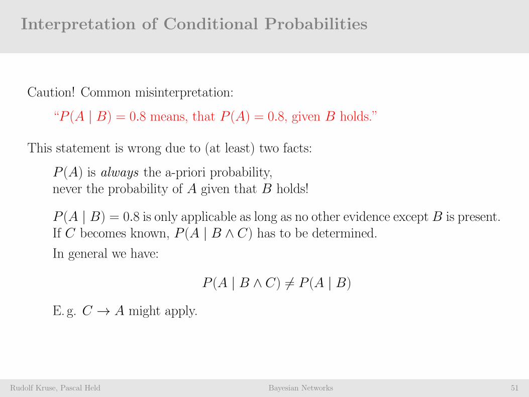
Caution! Common misinterpretation:

“P (A | B) = 0.8 means, that P (A) = 0.8, given B holds.”

This statement is wrong due to (at least) two facts:

P (A) is always the a-priori probability,never the probability of A given that B holds!

P (A | B) = 0.8 is only applicable as long as no other evidence except B is present.If C becomes known, P (A | B ∧ C) has to be determined.

In general we have:

P (A | B ∧ C) 6= P (A | B)

E. g. C → A might apply.

Joint Probabilities


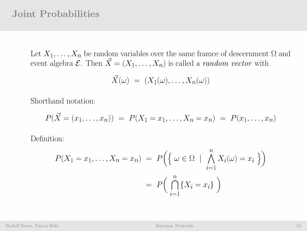
Let X1, . . . , Xn be random variables over the same framce of descernment Ω andevent algebra E . Then ~X = (X1, . . . , Xn) is called a random vector with

~X(ω) = (X1(ω), . . . , Xn(ω))

Shorthand notation:

P ( ~X = (x1, . . . , xn)) = P (X1 = x1, . . . , Xn = xn) = P (x1, . . . , xn)

Definition:

P (X1 = x1, . . . , Xn = xn) = P(

ω ∈ Ω |n∧

i=1

Xi(ω) = xi)

= P( n⋂

i=1

Xi = xi)

Joint Probabilities


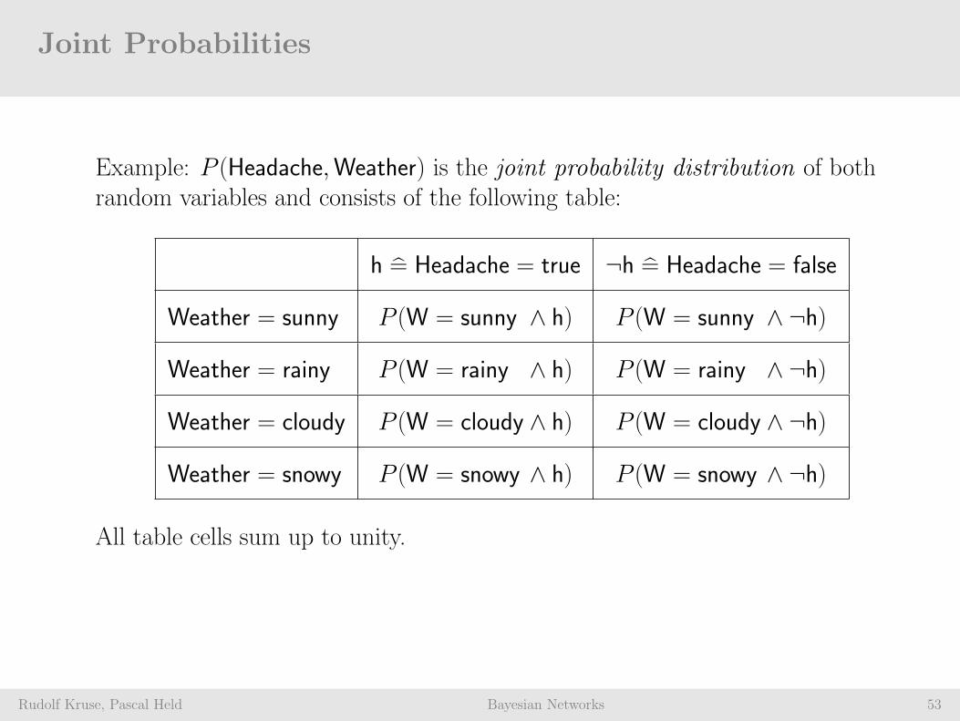
Example: P (Headache,Weather) is the joint probability distribution of bothrandom variables and consists of the following table:

h = Headache = true ¬h = Headache = false

Weather = sunny P (W = sunny ∧ h) P (W = sunny ∧ ¬h)

Weather = rainy P (W = rainy ∧ h) P (W = rainy ∧ ¬h)

Weather = cloudy P (W = cloudy ∧ h) P (W = cloudy ∧ ¬h)

Weather = snowy P (W = snowy ∧ h) P (W = snowy ∧ ¬h)

All table cells sum up to unity.

Calculating with Joint Probabilities


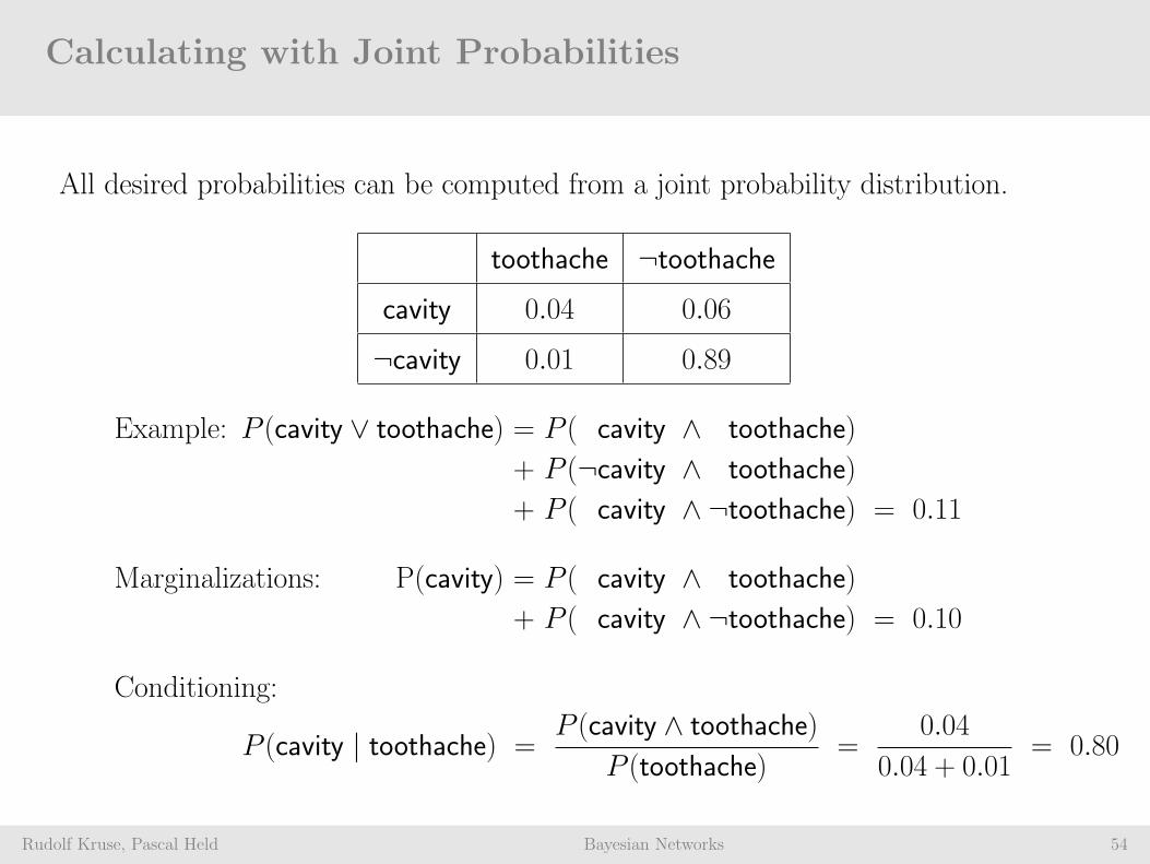
All desired probabilities can be computed from a joint probability distribution.

toothache ¬toothachecavity 0.04 0.06

¬cavity 0.01 0.89

Example: P (cavity ∨ toothache) = P ( cavity ∧ toothache)

+ P (¬cavity ∧ toothache)

+ P ( cavity ∧ ¬toothache) = 0.11

Marginalizations: P(cavity) = P ( cavity ∧ toothache)

+ P ( cavity ∧ ¬toothache) = 0.10

Conditioning:

P (cavity | toothache) =P (cavity ∧ toothache)

P (toothache)=

0.04

0.04 + 0.01= 0.80

Problems


Easiness of computing all desired probabilities comes at an unaffordable price:

Given n random variables with k possible values each, the joint probabilitydistribution contains kn entries which is infeasible in practical applications.

Hard to handle.

Hard to estimate.

Therefore:

1. Is there a more dense representation of joint probability distributions?

2. Is there a more efficient way of processing this representation?

The answer is no for the general case, however, certain dependencies and inde-pendencies can be exploited to reduce the number of parameters to a practicalsize.

Stochastic Independence


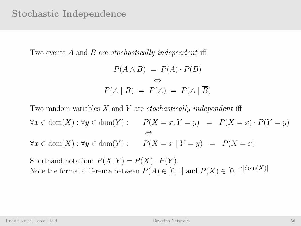
Two events A and B are stochastically independent iff

P (A ∧ B) = P (A) · P (B)

⇔P (A | B) = P (A) = P (A | B)

Two random variables X and Y are stochastically independent iff

∀x ∈ dom(X) : ∀y ∈ dom(Y ) : P (X = x, Y = y) = P (X = x) · P (Y = y)

⇔∀x ∈ dom(X) : ∀y ∈ dom(Y ) : P (X = x | Y = y) = P (X = x)

Shorthand notation: P (X, Y ) = P (X) · P (Y ).

Note the formal difference between P (A) ∈ [0, 1] and P (X) ∈ [0, 1]|dom(X)|.

Conditional Independence


Let X , Y and Z be three random variables. We call X and Y conditionallyindependent given Z, iff the following condition holds:

∀x ∈ dom(X) : ∀y ∈ dom(Y ) : ∀z ∈ dom(Z) :

P (X = x, Y = y | Z = z) = P (X = x | Z = z) · P (Y = y | Z = z)

Shorthand notation: X ⊥⊥P Y | Z

Let X = A1, . . . , Ak, Y = B1, . . . , Bl and Z = C1, . . . , Cm be threedisjoint sets of random variables. We call X and Y conditionally independentgiven Z, iff

P (X,Y | Z) = P (X | Z) · P (Y | Z)⇔ P (X | Y ,Z) = P (X | Z)

Shorthand notation: X ⊥⊥P Y | Z

Conditional Independence


The complete condition for X ⊥⊥P Y | Z would read as follows:

∀a1 ∈ dom(A1) : · · · ∀ak ∈ dom(Ak) :

∀b1 ∈ dom(B1) : · · · ∀bl ∈ dom(Bl) :

∀c1 ∈ dom(C1) : · · · ∀cm ∈ dom(Cm) :

P (A1 = a1, . . . , Ak = ak, B1 = b1, . . . , Bl = bl | C1 = c1, . . . , Cm = cm)

= P (A1 = a1, . . . , Ak = ak | C1 = c1, . . . , Cm = cm)

· P (B1 = b1, . . . , Bl = bl | C1 = c1, . . . , Cm = cm)

Remarks:

1. If Z = ∅ we get (unconditional) independence.2. We do not use curly braces () for the sets if the context is clear. Likewise,

we use X instead of X to denote sets.

Conditional Independence — Example 1


Y

X

t t

t

t

t

t

t

tt

tt

t

t

t

tt

t

t

t

t

t

t

t

t

t t

t

t

t

t

t

t

tt

t

t

t

t

tt

t

t

t

t

t

t t

t

tt

t

t

tt

t

t

t

t

t

t

t

t

t

t

t tt

t

t

t

t

tt

t

t

t

t

t

t

tt

tt

t

t

t

t

t

t

t

tt t

t

tt

t

t

t

t

t

t t

t

tt

t

tt

t

t

t

t

t

ttt

t

t

t

tt

t

tt

t

t

t

t

t

t

tt

t

t

t

t ttt

tt

t t

t

t

t t

t

t tt

t

t

t

t

t

t

t

t

t

t

t

t

t

tt

t

t

t

t

t

t

t

t

t

t

t

t

t

t

t

t

tt

t

tt

t

t

t

tt

t

t

tt

t

tt

Group 1

t

t

t

t

t

t

t

t

t

t

t

t

t

t

t

t

t

t

t

t

tt

t

t

tt t

tt

t

tt

t

t

t

t

t

t

t

tt

t

t

t

t

t

t

tt

t

t

t

t

t

t

t

t

t

t

tt

tt

t

ttt

tt t t

ttt

t

t

t

t

t

t

ttt

t

t

tt

t

tt

tt

t

t

t

t

t

t

tt

t

t

t

t

tt

t

t

t

t

t

t tt

t

tt

tt

tt

t

ttt

t

t t

t

t

t

t

tt

t tt

t

t

t

t t

t

t

t

tt

t

tt

t

t

t

t

t

t

t

t

t

t

tt

t

tt

t

t

t

t

tt

ttt

t

t

t

t

t

t

t

t

t

tt

t

t

t

t

t

t

t

t

t

t

t

t

t

t

t

Group 2

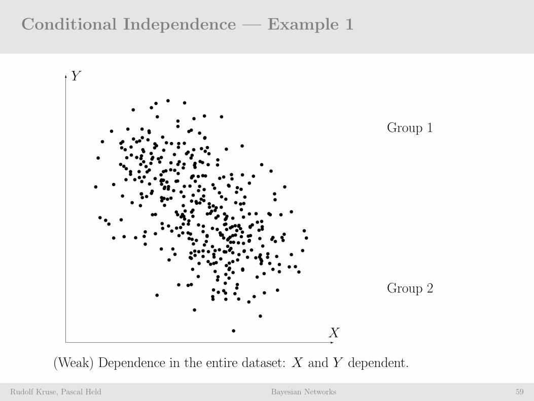
(Weak) Dependence in the entire dataset: X and Y dependent.



Y

X

t t

t

t

t

t

t

tt

tt

t

t

t

tt

t

t

t

t

t

t

t

t

t t

t

t

t

t

t

t

tt

t

t

t

t

tt

t

t

t

t

t

t t

t

tt

t

t

tt

t

t

t

t

t

t

t

t

t

t

t tt

t

t

t

t

tt

t

t

t

t

t

t

tt

tt

t

t

t

t

t

t

t

tt t

t

tt

t

t

t

t

t

t t

t

tt

t

tt

t

t

t

t

t

ttt

t

t

t

tt

t

tt

t

t

t

t

t

t

tt

t

t

t

t ttt

tt

t t

t

t

t t

t

t tt

t

t

t

t

t

t

t

t

t

t

t

t

t

tt

t

t

t

t

t

t

t

t

t

t

t

t

t

t

t

t

tt

t

tt

t

t

t

tt

t

t

tt

t

tt

Group 1

No Dependence in Group 1: X and Y conditionally independent given Group 1.



Y

X

t

t

t

t

t

t

t

t

t

t

t

t

t

t

t

t

t

t

t

t

tt

t

t

tt t

tt

t

tt

t

t

t

t

t

t

t

tt

t

t

t

t

t

t

tt

t

t

t

t

t

t

t

t

t

t

tt

tt

t

ttt

tt t t

ttt

t

t

t

t

t

t

ttt

t

t

tt

t

tt

tt

t

t

t

t

t

t

tt

t

t

t

t

tt

t

t

t

t

t

t tt

t

tt

tt

tt

t

ttt

t

t t

t

t

t

t

tt

t tt

t

t

t

t t

t

t

t

tt

t

tt

t

t

t

t

t

t

t

t

t

t

tt

t

tt

t

t

t

t

tt

ttt

t

t

t

t

t

t

t

t

t

tt

t

t

t

t

t

t

t

t

t

t

t

t

t

t

t

Group 2

No Dependence in Group 2: X and Y conditionally independent given Group 2.



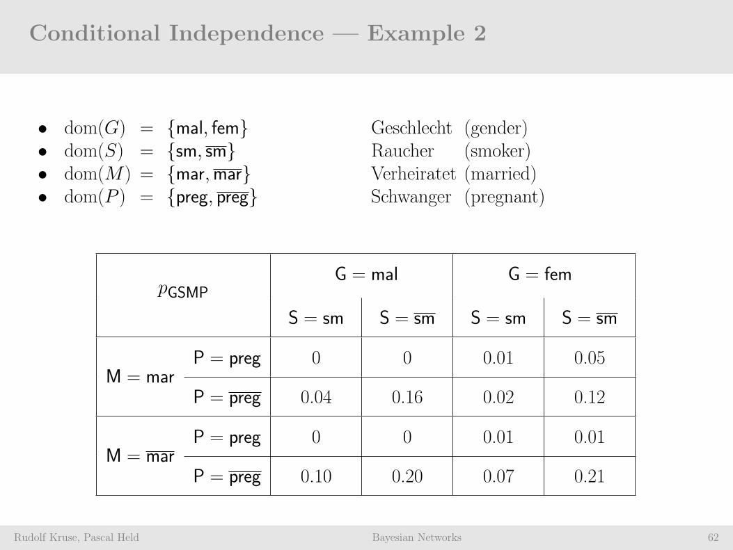
• dom(G) = mal, fem Geschlecht (gender)• dom(S) = sm, sm Raucher (smoker)• dom(M) = mar,mar Verheiratet (married)• dom(P ) = preg, preg Schwanger (pregnant)

pGSMPG = mal G = fem

S = sm S = sm S = sm S = sm

M = marP = preg 0 0 0.01 0.05

P = preg 0.04 0.16 0.02 0.12

M = marP = preg 0 0 0.01 0.01

P = preg 0.10 0.20 0.07 0.21



P (G= fem) = P (G=mal) = 0.5 P (P=preg) = 0.08

P (S= sm) = 0.25 P (M=mar) = 0.4

Gender and Smoker are not independent:

P (G= fem | S= sm) = 0.44 6= 0.5 = P (G= fem)

Gender and Marriage are marginally independent butconditionally dependent given Pregnancy:

P (fem,mar | preg) ≈ 0.152 6= 0.169 ≈ P (fem | preg) · P (mar | preg)

Bayes Theorem


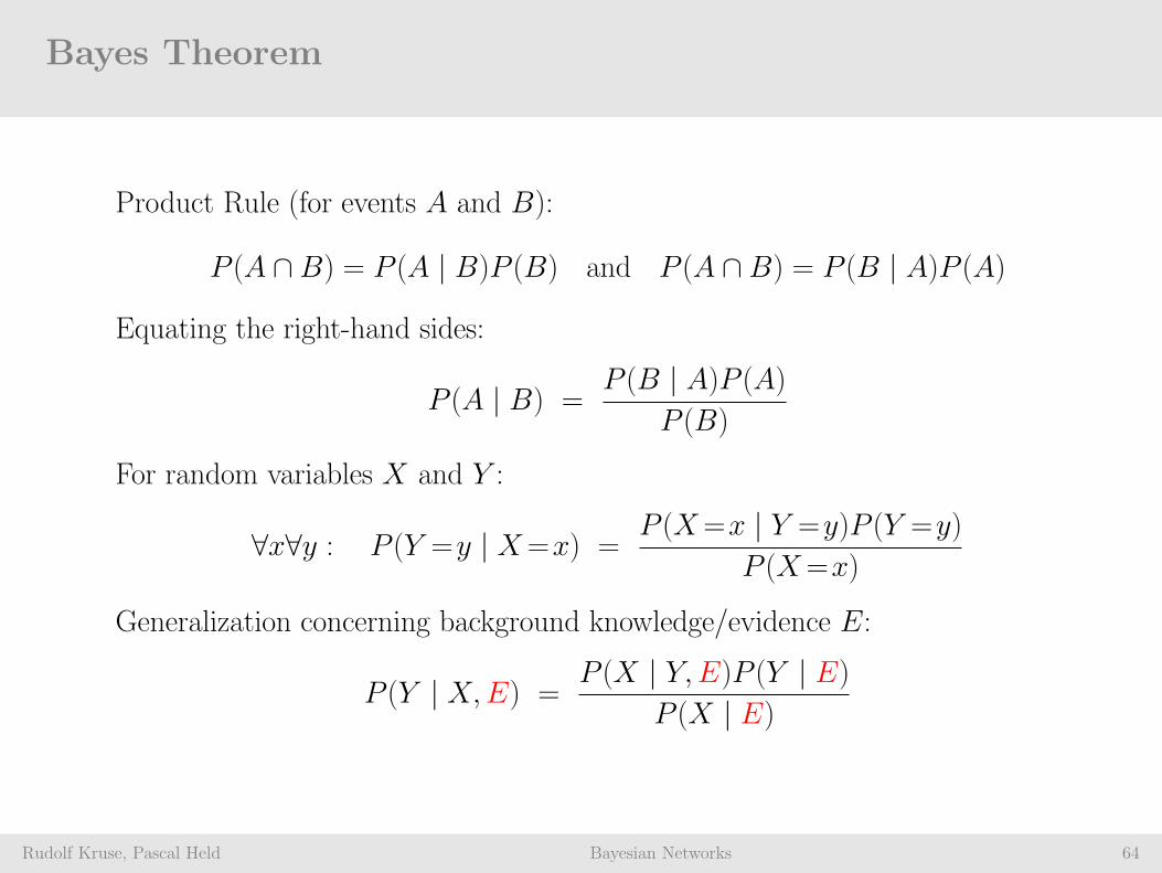
Product Rule (for events A and B):

P (A ∩ B) = P (A | B)P (B) and P (A ∩B) = P (B | A)P (A)

Equating the right-hand sides:

P (A | B) =P (B | A)P (A)

P (B)

For random variables X and Y :

∀x∀y : P (Y =y | X=x) =P (X=x | Y =y)P (Y =y)

P (X=x)

Generalization concerning background knowledge/evidence E:

P (Y | X,E) =P (X | Y,E)P (Y | E)

P (X | E)

Bayes Theorem — Application


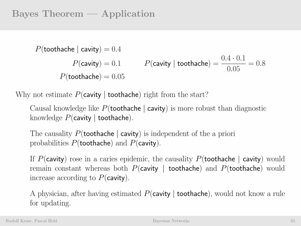
P (toothache | cavity) = 0.4

P (cavity) = 0.1 P (cavity | toothache) = 0.4 · 0.10.05

= 0.8

P (toothache) = 0.05

Why not estimate P (cavity | toothache) right from the start?

Causal knowledge like P (toothache | cavity) is more robust than diagnosticknowledge P (cavity | toothache).

The causality P (toothache | cavity) is independent of the a prioriprobabilities P (toothache) and P (cavity).

If P (cavity) rose in a caries epidemic, the causality P (toothache | cavity) wouldremain constant whereas both P (cavity | toothache) and P (toothache) wouldincrease according to P (cavity).

A physician, after having estimated P (cavity | toothache), would not know a rulefor updating.

Bayes Theorem — Using absolute Numbers


P (toothache | cavity) = 0.4 P (cavity) = 0.1

P (toothache | ¬cavity) = 190 P (cavity | toothache) = 40

40 + 10= 0.8

1000 people

100 cavity 900 ¬cavity

40 toothache 60 ¬toothache 10 toothache 890 ¬toothache

P (C | T ) = P (T | C) · P (C)P (T )

=P (T | C) · P (C)

P (T | C) · P (C) + P (T | ¬C) · P (¬C)

Relative Probabilities


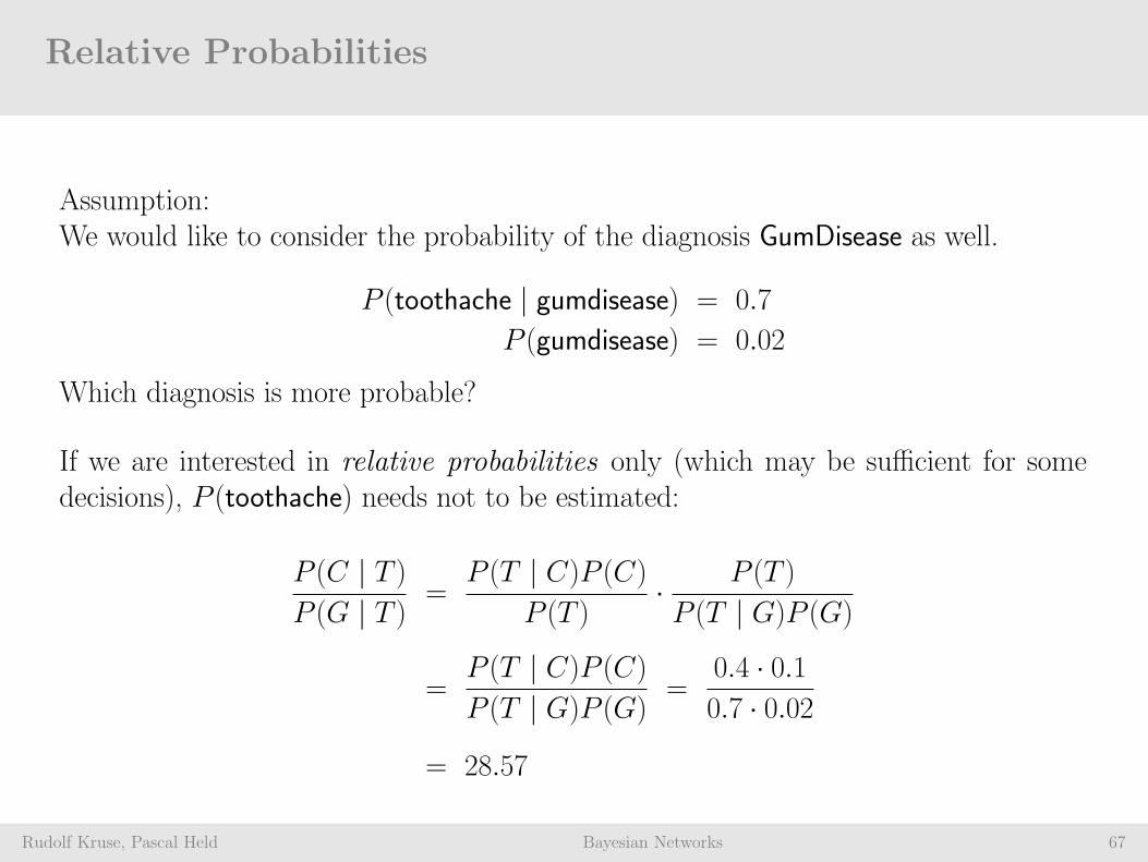
Assumption:We would like to consider the probability of the diagnosis GumDisease as well.

P (toothache | gumdisease) = 0.7

P (gumdisease) = 0.02

Which diagnosis is more probable?

If we are interested in relative probabilities only (which may be sufficient for somedecisions), P (toothache) needs not to be estimated:

P (C | T )P (G | T ) =

P (T | C)P (C)P (T )

· P (T )

P (T | G)P (G)

=P (T | C)P (C)P (T | G)P (G) =

0.4 · 0.10.7 · 0.02

= 28.57

Normalization


If we are interested in the absolute probability of P (C | T ) but do not know P (T ),we may conduct a complete case analysis (according C) and exploit the fact thatP (C | T ) + P (¬C | T ) = 1.

P (C | T ) =P (T | C)P (C)

P (T )

P (¬C | T ) =P (T | ¬C)P (¬C)

P (T )

1 = P (C | T ) + P (¬C | T ) =P (T | C)P (C)

P (T )+

P (T | ¬C)P (¬C)P (T )

P (T ) = P (T | C)P (C) + P (T | ¬C)P (¬C)

Normalization


Plugging into the equation for P (C | T ) yields:

P (C | T ) = P (T | C)P (C)P (T | C)P (C) + P (T | ¬C)P (¬C)

For general random variables, the equation reads:

P (Y =y | X=x) =P (X=x | Y =y)P (Y =y)

∑

∀y′∈dom(Y )

P (X=x | Y =y′)P (Y =y′)

Note the “loop variable” y′. Do not confuse with y.

Multiple Evidences


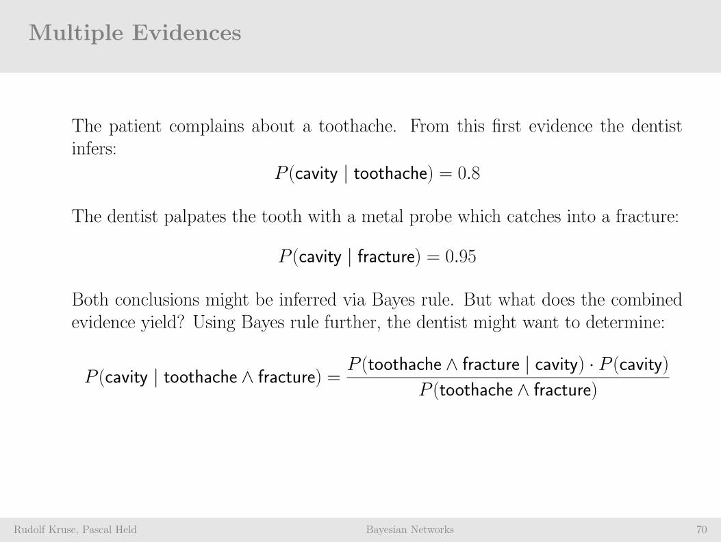
The patient complains about a toothache. From this first evidence the dentistinfers:

P (cavity | toothache) = 0.8

The dentist palpates the tooth with a metal probe which catches into a fracture:

P (cavity | fracture) = 0.95

Both conclusions might be inferred via Bayes rule. But what does the combinedevidence yield? Using Bayes rule further, the dentist might want to determine:

P (cavity | toothache ∧ fracture) =P (toothache ∧ fracture | cavity) · P (cavity)

P (toothache ∧ fracture)

Multiple Evidences


Problem:He needs P (toothache∧catch | cavity), i. e. diagnostics knowledge for all combinationsof symptoms in general. Better incorporate evidences step-by-step:

P (Y | X,E) =P (X | Y,E)P (Y | E)

P (X | E)

Abbreviations:

C — cavity

T — toothache

F — fracture

C

T F

Objective:Computing P (C | T, F ) with just using information about P ( · | C) and underexploitation of independence relations among the variables.

Multiple Evidences


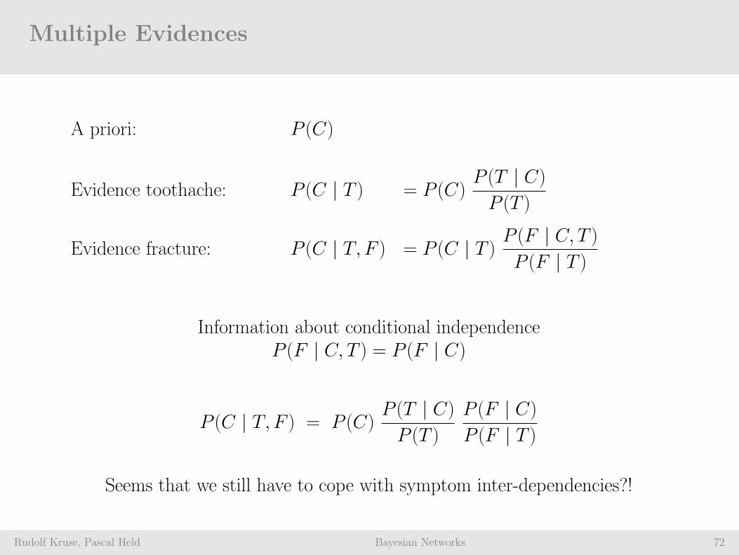
A priori: P (C)

Evidence toothache: P (C | T ) = P (C)P (T | C)P (T )

Evidence fracture: P (C | T, F ) = P (C | T ) P (F | C, T )P (F | T )

Information about conditional independenceP (F | C, T ) = P (F | C)

P (C | T, F ) = P (C)P (T | C)P (T )

P (F | C)P (F | T )

Seems that we still have to cope with symptom inter-dependencies?!

Multiple Evidences


Compound equation from last slide:

P (C | T, F ) = P (C)P (T | C) P (F | C)P (T ) P (F | T )

= P (C)P (T | C) P (F | C)

P (F, T )

P (F, T ) is a normalizing constant and can be computedif P (F | ¬C) and P (T | ¬C) are known:

P (F, T ) = P (F, T | C)︸︷︷︸P (F |C)P (T |C)

P (C) + P (F, T | ¬C)︸︷︷︸P (F |¬C)P (T |¬C)

P (¬C)

Therefore, we finally arrive at the following solution...

Multiple Evidences


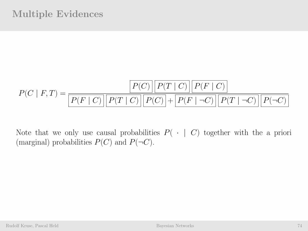
P (C | F, T ) =P (C) P (T | C) P (F | C)

P (F | C) P (T | C) P (C) + P (F | ¬C) P (T | ¬C) P (¬C)

Note that we only use causal probabilities P ( · | C) together with the a priori(marginal) probabilities P (C) and P (¬C).

Multiple Evidences — Summary


Multiple evidences can be treated by reduction on

a priori probabilities

(causal) conditional probabilities for the evidence

under assumption of conditional independence

General rule:

P (Z | X, Y ) = α P (Z) P (X | Z) P (Y | Z)

for X and Y conditionally independent given Z and with normalizing constant α.

Monty Hall Puzzle


Marylin Vos Savant in her riddle column in the New York Times:

You are a candidate in a game show and have to choose between three doors. Behindone of them is a Porsche, whereas behind the other two there are goats. After you chosea door, the host Monty Hall (who knows what is behind each door) opens another (notyour chosen one) door with a goat. Now you have the choice between keeping yourchosen door or choose the remaining one.

Which decision yields the best chance of winning the Porsche?

Monty Hall Puzzle


G You win the Porsche.

R You revise your decision.

A Behind your initially chosen door is (and remains) the Porsche.

P (G | R) = P (G,A | R) + P (G,A | R)= P (G | A,R)P (A | R) + P (G | A,R)P (A | R)= 0 · P (A | R) + 1 · P (A | R)

= P (A | R) = P (A) =2

3

P (G | R) = P (G,A | R) + P (G,A | R)= P (G | A,R)P (A | R) + P (G | A,R)P (A | R)= 1 · P (A | R) + 0 · P (A | R)

= P (A | R) = P (A) =1

3

Simpson’s Paradox


Example: C = Patient takes medication, E = patient recovers

E ¬E ∑Recovery rate

C 20 20 40 50%¬C 16 24 40 40%∑

36 44 80

Men E ¬E ∑Rec.rate Women E ¬E ∑

Rec.rateC 18 12 30 60% C 2 8 10 20%¬C 7 3 10 70% ¬C 9 21 30 30%

25 15 40 11 29 40

P (E | C) > P (E | ¬C)but P (E | C,M) < P (E | ¬C,M)

P (E | C,W ) < P (E | ¬C,W )

Excursus: Focusing vs. Revision


Philosophical topic, studied e.g. by Kant, Gardenfors

Example for Focusing

Prior knowledge: fair die

New evidence: the result is an odd number

Aposteriori knowledge via focusing: conditional probability

Underlying probability measure did not change

Example for Revision

Prior knowledge: fair die

New evidence: weight near the 6

Belief change via revision

Underlying probability measure did change

Excursus: Causality vs. Correlation


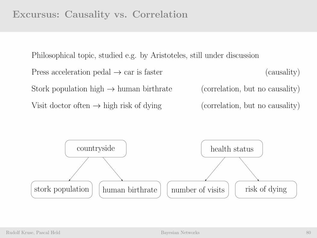
Philosophical topic, studied e.g. by Aristoteles, still under discussion

Press acceleration pedal → car is faster (causality)

Stork population high → human birthrate (correlation, but no causality)

Visit doctor often → high risk of dying (correlation, but no causality)

countryside

stork population human birthrate

health status

number of visits risk of dying

Probabilistic Reasoning


Probabilistic reasoning is difficult and may be problematic:

P (A ∧ B) is not determined simply by P (A) and P (B):P (A) = P (B) = 0.5 ⇒ P (A ∧ B) ∈ [0, 0.5]

P (C | A) = x, P (C | B) = y ⇒ P (C | A ∧ B) ∈ [0, 1]Probabilistic logic is not truth functional !

Central problem: How does additional information affect the current knowledge?I. e., if P (B | A) is known, what can be said about P (B | A ∧ C)?

High complexity: n propositions → 2n full conjunctives

Hard to specify these probabilities.

Summary


Uncertainty is inevitable in complex and dynamic scenariosthat force agents to cope with ignorance.

Probabilities express the agent’s inability to vote for adefinitive decision. They model the degree of belief.

If an agent violates the axioms of probability, it may exhibitirrational behavior in certain circumstances.

The Bayes rule is used to derive unknown probabilities frompresent knowledge and new evidence.

Multiple evidences can be effectively included into computationsexploiting conditional independencies.

Date post:	15-Feb-2022
Category:	Documents
Upload:	others
View:	1 times
Download:	0 times

Probability Foundations

Documents