Probability Models for Targeted Borrowing of Information by P. Richard Hahn Department of Statistical Science Duke University Date: Approved: Sayan Mukherjee, Supervisor Carlos Carvalho David Dunson Mike West Dissertation submitted in partial fulfillment of the requirements for the degree of Doctor of Philosophy in the Department of Statistical Science in the Graduate School of Duke University 2011
Transcript
Probability Models for Targeted Borrowing of
Information
by
P. Richard Hahn
Department of Statistical ScienceDuke University
Date:
Approved:
Sayan Mukherjee, Supervisor
Carlos Carvalho
David Dunson
Mike West
Dissertation submitted in partial fulfillment of the requirements for the degree ofDoctor of Philosophy in the Department of Statistical Science
in the Graduate School of Duke University2011
Abstract(Statistics)
Probability Models for Targeted Borrowing of Information
by
P. Richard Hahn
Department of Statistical ScienceDuke University
Date:
Approved:
Sayan Mukherjee, Supervisor
Carlos Carvalho
David Dunson
Mike West
An abstract of a dissertation submitted in partial fulfillment of the requirements forthe degree of Doctor of Philosophy in the Department of Statistical Science
2.1 Mean Stein and Frobenius losses suffered in reconstructing the truecorrelation matrix R in various configurations. . . . . . . . . . . . . . 25
2.2 Posterior summaries for the 19 closest Senate votes in the 95th Congress.The first line of the table reflects a pseudo-vote as to whether theSenator was a Democrat (1) or Republican (0), which we took as thefounder of the first factor. We have annotated several other votes toreflect the general issue at stake; this aids in interpreting the factors.The number in brackets after the issue reflects the chronological orderof votes for the two-year period in question. . . . . . . . . . . . . . . 35
3.1 PFR: Partial factor regression. NIG: conjugate prior linear regression.BFR: Bayesian factor regression. Both the factor model and the par-tial factor model selected k a priori by looking at the singular valuesof design matrix, so that the top k singular vectors account for 90%of the observed variance. . . . . . . . . . . . . . . . . . . . . . . . . . 55
3.2 PFR: partial factor regression. RR: ridge regression. PLS: partialleast squares. LARS: least angle regression. PCR: principal compo-nent regression. Percentages shown are amount worse than the bestmethod, reported in bold type. . . . . . . . . . . . . . . . . . . . . . 57
2.1 Comparison of the sparse versus non-sparse models in terms of theirinduced priors on correlation coefficients and percentage of variationexplained by the factors. . . . . . . . . . . . . . . . . . . . . . . . . . 20
2.2 Left: The loadings matrix of each scotch upon the three latent factors.Note how the sparsity prior yields factor loadings on the first factorthat easily identify it as the “single malt” factor. Right: 90% posteriorcredible intervals for the percent variation in each scotch explained bycommon factors, with the remainder explained idiosyncratically. . . . 27
2.3 The first two mean eigenvectors of the implied correlation matrix.Compare to Figure 3 of Edwards and Allenby (2003). . . . . . . . . . 28
2.4 The most partisan voter of each of the past 30 congresses, orderedconsecutively. The height of each bar represents the posterior meanof the respective Senators’ first factor score. Familiar names on thislist help to build confidence in the model. . . . . . . . . . . . . . . . . 32
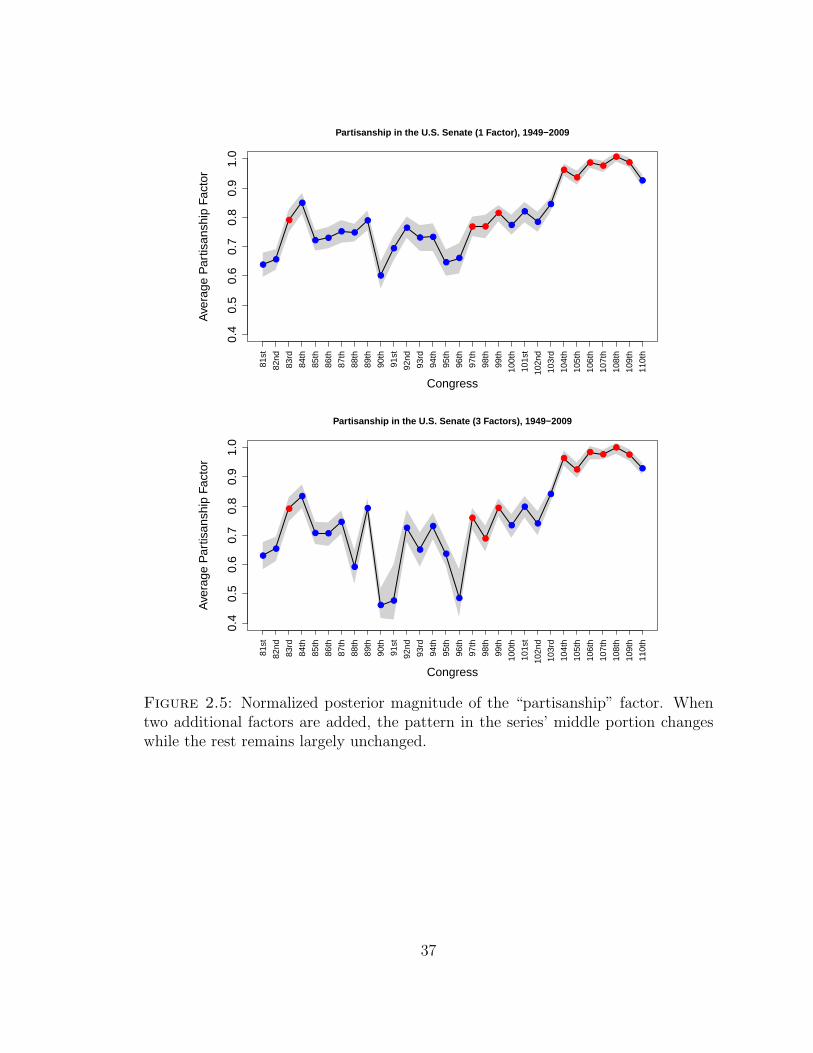
2.5 Normalized posterior magnitude of the “partisanship” factor. Whentwo additional factors are added, the pattern in the series’ middleportion changes while the rest remains largely unchanged. . . . . . . 37
3.1 Points denote realizations from the true two-factor model. For pointsabove the dashed horizontal line, the likelihood ratio favors the truemodel. The distance to the right of the dashed vertical line measureshow much worse than the true model the one-factor approximation didin terms of predicting X10. Model selection based on the full likelihoodfavors the larger model half the time, while model selection based onpredictive fit favors the larger model nearly always. . . . . . . . . . . 44
4.1 Strategic play is not overwhelmingly apparent from the raw data,which appears roughly uniform. We have rescaled here to the unitinterval (as we will throughout). . . . . . . . . . . . . . . . . . . . . . 71
xii
4.2 Lines connect players’ bids across games with differing levels of α.This plot illustrates valid CH play wherein individuals do not switchmixture component/strategy class across games. . . . . . . . . . . . . 80
4.3 Switching class across α, as shown here, is not permitted under a CHmodel. . . . . . . . . . . . . . . . . . . . . . . . . . . . . . . . . . . 80
4.4 Six vertical lines mark the bidding distribution at the α level of thecorresponding histogram. Line segments link players’ bids across thevarious values. The bidding behavior across rounds appears largelyhaphazard. . . . . . . . . . . . . . . . . . . . . . . . . . . . . . . . . . 81
4.5 By contrast, simulated data drawn from a CH-Poisson model (withτ 1, Beta errors and a level-0 mean play of 0.85) exhibits clearstructure, with clustering of bids that is consistent across α levels anda general upward trend of those clusters as α increases. . . . . . . . 82
4.6 These draws from the SPCH prior demonstrate the key feature ofevolving together to maintain the relevant order restrictions on thetarget bids across four levels of α. Each panel shows a single four-component pK 4q mixture density over four values of α ascendingfrom green to pink to orange to gray. . . . . . . . . . . . . . . . . . . 86
4.7 By contrast, these draws from the null latent class distribution clearlydisplay non-order-restricted cluster means. . . . . . . . . . . . . . . . 86
4.8 After fitting a four-class SPCH model, we can partition the playerpopulation by estimated modal class membership. This results inthree populated strategy classes. Qualitatively this corresponds to arandom class, and one and two step-ahead thinkers. . . . . . . . . . . 90
5.1 Posterior πY pθq (red) based on Jeffreys’ substitution likelihood for θthe 30th percentile. In this example n 20, the prior was Np0, σ2qwith σ 4 (black) and observations are i.i.d. Np3, 16q. The true quan-tile is given by 4Φ1p0.3q3 (approximately 0.9). The discontinuitiesoccur at the observed data points; note that within each partition theshape of the density remains unchanged from the prior, reflecting theflatness of the pseudo-likelihood within each region. . . . . . . . . . . 99
5.2 Histogram of draws from an asymmetric Laplace distribution withλz 3 and λv 1. Note the discontinuity at the “seam”. . . . . . . . 101
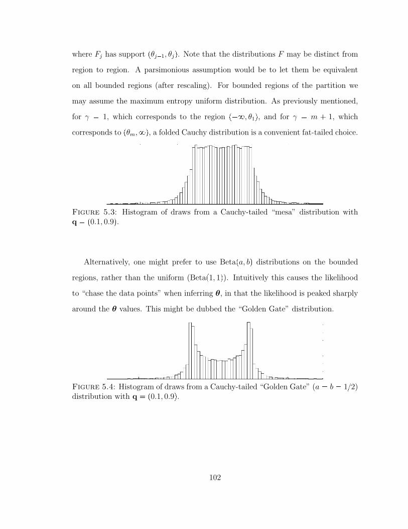
5.3 Histogram of draws from a Cauchy-tailed “mesa” distribution withq p0.1, 0.9q. . . . . . . . . . . . . . . . . . . . . . . . . . . . . . . . 102
xiii
5.4 Histogram of draws from a Cauchy-tailed “Golden Gate” (a b 12) distribution with q p0.1, 0.9q. . . . . . . . . . . . . . . . . . . . 102
5.5 For n 150 the left panel shows the posterior mean regression linesin magenta. The true regression lines are shown in blue at right. Theobserved data is superimposed in green. . . . . . . . . . . . . . . . . . 104
5.6 Example of three accounting time series: red is return on assets (ROA),green is total shareholder return (TSR) and blue is growth. All num-bers have been standardized. Note that trending and covariation aredifficult to perceive. . . . . . . . . . . . . . . . . . . . . . . . . . . . . 108
5.7 In its observed state, the three sequences may appear – even in thelow noise setting – to be related in terms of general trends but notnecessarily in every fluctuation. Once transformed by simple stretchesand shifts, the three series are seen to be subsequences of the samelatent trajectory. . . . . . . . . . . . . . . . . . . . . . . . . . . . . . 109
5.8 With minimal additive noise, plotting one series against the otherbetrays the one-dimensional manifold structure. A continuous curvein the plane emerges. . . . . . . . . . . . . . . . . . . . . . . . . . . . 110
xiv
List of Abbreviations and Symbols
Commonly referenced distributions
Npµ, σ2q The Normal or Gaussian distribution.
ppy | µ, σ2q p2πσ2q12 exppy µq22σ2
.
MVNpµ,Σq The p-dimensional multivariate Normal distribution.
ppY | µ,Σq p2πqp2|Σ|12 exp
pY µqtΣ1pY µq2
.
IGpa, bq The Inverse-Gamma distribution.
ppy | a, bq ba
Γpaqypa1q exp pbyq.
Betapa, bq The Beta distribution.
ppy | a, bq Γpa bq
ΓpaqΓpbqypa1qp1 yqpb1q.
Upa, bq The uniform distribution.
ppy | a, bq 1pb aq.
xv
Acknowledgements
First, I thank Emil J. Font for supporting me unswervingly during the whole of my
education, from grammar school to this day. I thank Laura Suhr, Melissa Wong,
Chad DeChant and Shira Katseff for permitting my social life to be chock full of
wonky science and philosophy discussions.
I thank the mathematics faculty of New Mexico Institute of Mining and Technol-
ogy and especially Professor Brian Borchers for providing me guidance and support
early in my graduate career. From my time in New Mexico I thank Norelle Shlanta
and Xian and Danielle Lucero for providing me with warm meals and companionship.
In Durham, thanks likewise to Aunt Sue and Uncle Victor.
I want to thank David Banks and Sayan Mukherjee for helping see me through
a not-always-smooth first year. Thanks to Deepak Agarwal at Yahoo! research;
working with him the summer after my first year was an experience that shaped my
whole approach to statistical modeling. I thank Mike West for his 214 class, which
is the finest course I have ever taken. I thank David Dunson for patiently overseeing
my prelim project and for bringing a vital intensity to our department.
I especially thank my two closest advisors: Sayan Mukherjee and Carlos Carvalho.
I very literally could not have done this work without them. I have appreciated their
support and enjoyed their company these past years. I also thank Carl Mela, the
“fifth man” of my committee, for providing counsel the past two years and being an
excellent advisor in everything but name.
xvi
I must also thank my peers in the department over the years: Jarad Niemi, Eric
Vance, Simon Lunagomez, Kristian Lum, Melanie Wilson, Jeff Sipe, Matt Heaton,
Ken van Haren, Jared Murray, and Andrew Cron. Special thanks go to James Scott,
Dan Merl, Ioanna Manolopoulou, and Lane Burgette, who bore the brunt of my
constant shoptalk.
Thanks also to the Booth School of Business and to the NSF and Duke’s Math-
ematical Biology Research Training Grant (NSF-DMS-0943760).
Finally, I express my eternal gratitude to Shira Katseff, for putting up with me,
for being my closest ally and greatest role model, my primary source of amusement
and my most steady source of consolation, and for generally helping me get along in
life.
xvii
1
Introduction
Modern science produces vast amounts of multivariate, correlated data, from ge-
nomics and proteomics to financial markets and social networks. The once-dominant
paradigm of statistical inference based on independent observations is plainly unsuit-
able for analyzing data of this type. A convenient approach for constructing more
appropriate multivariate models which are capable of capturing important dependen-
cies, is via the introduction of unobservable latent variables, conditional upon which
the observed data may be assumed independent. While this description could as
well describe a parameter of a statistical model, what distinguishes latent variables
is that they may be uniquely associated with each individual observation. This over-
parameterization is prevented from leading to over-fitting via the use of hierarchical
modeling, meaning that the latent factors are assumed to arise as draws from a given
prior distribution. Complex dependence structure can emerge once the latent vari-
ables are integrated out of the model. This basic modeling strategy allows models
of a more realistic level of sophistication to be built up from standard components,
such as exponential family likelihood functions. Here, two of the most successful
models of this type are reviewed and the novel modifications which are the subject
1
of subsequent chapters are presented in outline.
1.1 Overview
1.1.1 Linear factor models
Given a p-by-k matrix B and a k-by-1 vector fi, a linear factor model for the p-
dimensional vector Yi takes the form
Yi Bfi εi
where εi is a p-dimensional, independent, additive error term; conditional on the
factors fi, the data may be viewed as realizations of an independent and identically
distributed random variable. However, the fi are never actually observed. The so-
called factor scores, fi, are then given some prior distribution G. Integrating over the
latent factors induces a stochastic dependence structure among the observed data.
In particular, by linearity
CovpYiq BCovpfiqBt Covpεiq,
where Covpεiq is assumed diagonal.
In the special case that fiiid Np0, Ikq and εi
iid Np0,Ψq the marginal distribution
of Yi is also Normally distributed:
Yi Np0,BBt Ψq.
Note that if k ¥ p 1, any positive definite matrix may be written in this form; the
more practically interesting case is when k ! p. This model – simply a multivariate
Gaussian distribution with a structured covariance matrix – will serve as the basis
for the work in chapters 2 and 3. Additional details about identification and model
fitting may be found in those chapters.
Factor models have been a topic of research for more than 100 years. A seminal
reference is Spearman (1904), while Press (1982) and Bartholomew (1987) are key
2
contemporary references. Bayesian factor models for continuous data have been
developed by many authors, including Geweke and Zhou (1996), Aguilar and West
(2000), and West (2003). A comprehensive bibliography may be found in Lopes
(2003).
Notable application areas include finance (Aguilar and West, 2000; Fama and
French, 1993; Fan et al., 2008; Bai, 2003; Chamberlain and Rothschild, 1983; Lopes
and Carvalho, 2007) and gene expression studies (Merl et al., 2009; Lucas et al.,
2006; Carvalho et al., 2008).
The subject continues to see new developments, in areas such as prior specification
(Ghosh and Dunson, 2009), model selection (Lopes and West, 2004; Bhattacharya
and Dunson, 2011) and identification (Fruhwirth-Schnatter and Lopes, 2009).
1.1.2 Latent mixture models
An m-component mixture model assumes that the density for vector Yi may be
written as
ppYi | πq m
j1
πjfjpYiq
for a collection of density function fjpq. The vector of mixture weights, π, satisfies°mj1 πj 1 and 0 ¤ πj ¤ 1 for all j. In practice it is common and convenient
to use a parametric family for these densities, whereupon they may be expressed as
fjpq fp | θjq with component-sepcific parameter θj. Note that it is possible to
use m 8, in which case one refers to an “infinite mixture model”.
This density representation can be written conveniently by augmenting with la-
tent indicator variables:
Prpγi jq πj
ppYi | γiq fγipYiq.
3
This formulation proves convenient conceptually and also (perhaps especially) com-
putationally in conjunction with the EM algorithm (Dempster et al., 1977) for maxi-
mum likelihood estimation or a Gibbs sampling approach (Gelfand and Smith, 1990)
for full posterior inference.
Estimation of mixture models is complicated by identification concerns. There
are two basic types of identifying restrictions that must be considered: permutation
of the indices of the mixture components and redundancy of individual mixture
components. The first issue can be routinely handled by imposing order restrictions
on the component-specific parameters (e.g., θj θk for j k). The second issue
arises when m is strictly larger than necessary to describe the data. This situation
can be handled either by allowing certain of the mixing weights to be exactly zero, or
by allowing certain of the component-specific parameters to be identical (e.g., θj θk
for some j k). These subtleties are not treated here; an in-depth discussion may
be found in McLachlan and Peel (2000).
The uses of mixture models are many, including density estimation (Escobar and
The multivariate probit model reduces the problem of estimating 2p probabilities
to the problem of estimating the ppp 1q2 pairwise correlations which comprise Σ.
The price of this reduction is the Normality assumption on the latent utilities, which
implies (among other things) a linear dependence structure. For many applications
these assumptions are unobjectionable, and indeed the multivariate probit model is
widely used (see, e.g., the examples discussed in Lesaffre and Molenberghs (1991)).
2.3.2 Gaussian factor models
While inference in a multivariate probit model is reduced to estimation of a correla-
tion matrix, this task is challenging in its own right. Standard estimators are liable
to be unstable when p is large compared to n, and can provide a distorted picture
of the eigenstructure of Σ (Sun and Berger, 2006). These difficulties are only com-
pounded in the multivariate probit model where the covariance matrix corresponds
to an unobserved random variable.
16
Here, we address this instability by imposing a regularizing factor structure, let-
ting
covpziq BBt Ψ, (2.3)
where Ψ is p-by-p diagonal with non-negative elements and rankpBq k p. We
may rewrite this model by augmenting the representation to include factor scores fi.
Conditional on B and fi the elements of zi are independent:
zi Bfi νi, ν Np0,Ψq
fi Np0, Ikq.(2.4)
For Σ BB1 Ψ to have a unique solution in B, i.e. for B to be identifiable,
constraints must be placed on B. These restrictions, discussed extensively in Aguilar
(1998), are distinct from the fact that Σ must be a correlation matrix in the probit
setting. In particular, two sorts of unidentifiability must be handled: sign indeter-
minacy and rotation indeterminacy. Traditional solutions to this problem include
forcing B to be orthogonal or BtΨB to be diagonal. Another approach (Geweke and
Zhou, 1996) is to constrain B to be zero for upper-triangular entries tbjk : k ¡ ju
(solving rotational indeterminacy) and positive along the diagonal tbjj ¡ 0u (solving
sign indeterminacy).
2.3.3 Latent factor probit models
Because Σ BBt Ψ is only identified up to a correlation matrix, we may fix
ψjj 1 for all j as is standard in the item-response-modeling literature (Johnson and
Albert, 1999). Priors on the elements bjk of B then induce a prior distribution on the
identifiable correlation coefficients ρjm for j m (Rossi et al., 2006). In this set-up,
the size of the elements of B describe the amount of the variation attributable to the
factor structure as opposed to idiosyncratic noise. The scale of the prior distribution
on these elements thus governs our prior expectations about the strength of the factor
structure in terms of describing the observed patterns of covariation.
17
2.3.4 Sparsity priors
A sparse model is one in which certain parameters are permitted to be exactly zero.
The canonical example is a linear model in which subsets of the regression coefficients
may be estimated to be zero. The sparsity framework spans the areas of regularized
prediction, hypothesis testing, and model selection, depending on whether it is viewed
as a means or as an end; for our purpose, it will serve both roles.
Likewise, sparsity can be achieved in a variety of ways, such as direct testing or
thresholding. Here we take an implicit testing approach via sparsity priors which
affix a point-mass probability at zero (George and McCulloch, 1993; Mitchell and
Beauchamp, 1988). A detailed discussion of this and similar Bayesian approaches
to model selection in linear regression can be found in Ishwaran and Rao (2005).
Our development closely follows West (2003) and Carvalho et al. (2008) who develop
sparse factor models for continuous data in the context of gene-expression studies.
These models assume that each latent factor will be associated with only a small
number of observed variables, yielding a more parsimonious covariance structure.
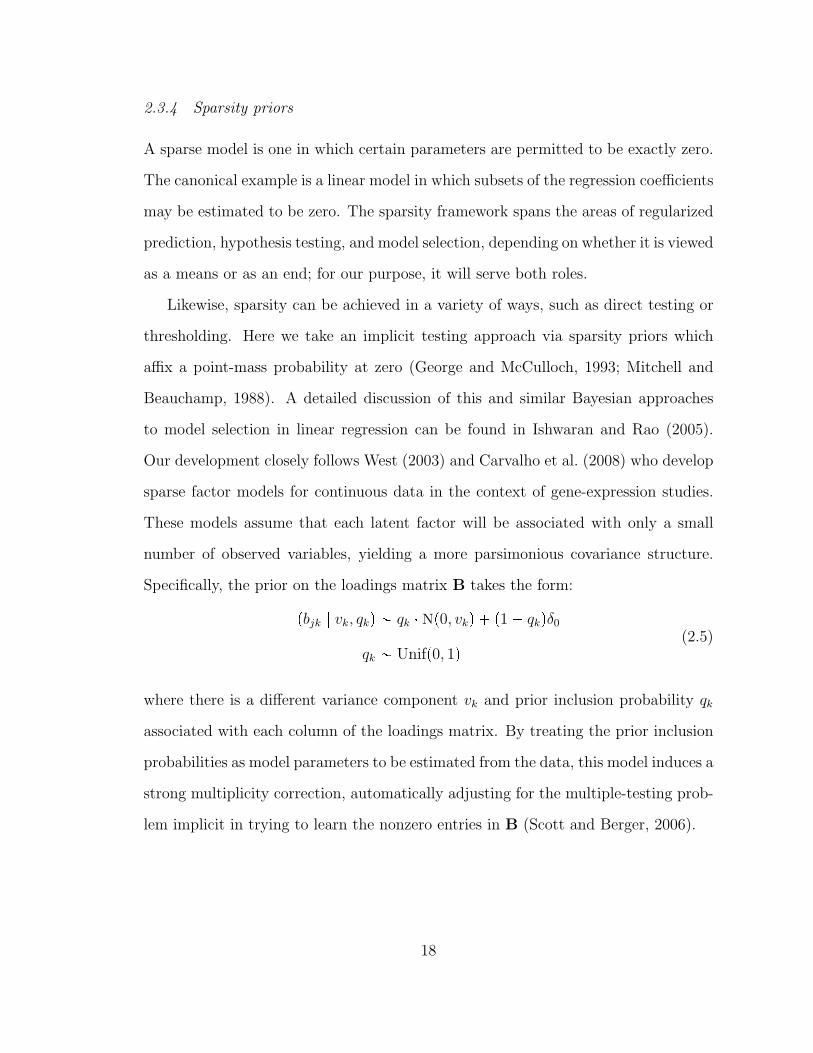
Specifically, the prior on the loadings matrix B takes the form:
pbjk | vk, qkq qk Np0, vkq p1 qkqδ0
qk Unifp0, 1q(2.5)
where there is a different variance component vk and prior inclusion probability qk
associated with each column of the loadings matrix. By treating the prior inclusion
probabilities as model parameters to be estimated from the data, this model induces a
strong multiplicity correction, automatically adjusting for the multiple-testing prob-
lem implicit in trying to learn the nonzero entries in B (Scott and Berger, 2006).
18
2.4 Sparse factor probit models
2.4.1 Prior choice
We now describe a novel sparse Bayesian factor-analytic probit model, where some
of the unconstrained elements in the factor-loadings matrix B can be identically 0.
In a sparse factor model, the pattern of non-zero elements in B is unknown and
must be estimated from the data. Previous authors have assumed, in the context of
continuous data, the model in (2.5), where there is a different variance component
vk and prior inclusion probability qk associated with each column of the loadings
matrix. At one extreme, entire columns of the loadings matrix can be set to exactly
zero with probability near one, effectively selecting the number of necessary factors
automatically.
We modify this now-standard model by grouping the variance components by row
rather than by column:
pbjk | vj, qkq qk Np0, vjψjq p1 qkqδ0
vj IGpc2, cd2q
qk Bep1, 1q .
(2.6)
This change reflects the fact that while the sparsity (that is, the fraction of exactly-
zero factor loadings) is naturally a factor-specific property, the variability of the
factor loadings should instead be a row-specific property. Intuitively, since binary
data are informative not about the raw scale of the zi’s, but only about the amount
of variation in the zi’s explained by the factors, the factor loadings are most naturally
scaled by row.
2.4.2 The effect of the sparsity prior
A considerable advantage of our approach is that sparsity allows for much more
flexible patterns of correlation structure than can be accommodated by ordinary
19
Draws from the sparse model
κκ3
Prio
r P
roba
bilit
y
0.0 0.2 0.4 0.6 0.8 1.0
0
0.1
0.2
Prior: c = 1, d = 1
ρρ23
Prio
r P
roba
bilit
y
−1.0 −0.5 0.0 0.5 1.0
0
0.1
0.2
0.3
0.4
Draws from the non−sparse model
κκ3
Prio
r P
roba
bilit
y
0.0 0.2 0.4 0.6 0.8 1.0
0
0.1
0.2
0.3
Prior: c = 1, d = 1
ρρ23
Prio
r P
roba
bilit
y−1.0 −0.5 0.0 0.5 1.0
0
0.1
Draws from the sparse model
κκ3
Prio
r P
roba
bilit
y
0.0 0.2 0.4 0.6 0.8 1.0
0
0.1
0.2
0.3
0.4
0.5
0.6
Prior: c = 0.1, d = 0.1
ρρ23
Prio
r P
roba
bilit
y
−1.0 −0.5 0.0 0.5 1.0
0
0.1
0.2
0.3
0.4
Draws from the non−sparse model
κκ3
Prio
r P
roba
bilit
y
0.0 0.2 0.4 0.6 0.8 1.0
0
0.1
0.2
0.3
0.4
0.5
0.6
Prior: c = 0.1, d = 0.1
ρρ23
Prio
r P
roba
bilit
y
−1.0 −0.5 0.0 0.5 1.0
0
0.1
0.2
Figure 2.1: Comparison of the sparse versus non-sparse models in terms of theirinduced priors on correlation coefficients and percentage of variation explained bythe factors.
20
factor-probit models. To illustrate this, we show how the sparsity prior changes the
induced prior on two key quantities of interest: the correlation coefficient between
two elements of z, denoted ρij; and the percentage of variation in the jth margin of
z that is explained by the factors,
κj B1jBjpB
1jBj Ψjq .
Here B1j is the row of the factor loadings matrix corresponding to component j of
the random vector z.
For the sake of illustration, we considered a three-factor model with five compo-
nents in z, and simulated data both with and without sparsity in B. Figure 2.1 show
histograms of the marginal priors on κ3 and ρ2,3 for different values of the hyperpa-
rameters c and d that govern the prior variance vj for the coefficients in row j of the
factor loadings matrix. The first two plots display the implied priors without the
additional sparsity component; the second plots two show the implied priors with
the sparsity component.
As the figures show, the sparsity component permits shrinking away from mod-
erate correlation—that is, towards zero correlation or very strong correlation, either
positive or negative. On the one hand, in the extreme case of the prior where c 0.1
and d 0.1, we observe that the correlation coefficient can be given a marginal prior
with three modes at the extreme values of 1, 0, and 1. This may be useful for
exploratory purposes, such as identifying highly parsimonious regimes. On the other
hand, the c 1, d 1 prior is perhaps a more reasonable default choice reflecting
plausibly realistic prior beliefs across a broad range of data. Here we observe that the
sparsity prior adds a local mode at zero for κ3, a feature that is virtually impossible
without simultaneously concentrating the prior probability mass of the correlation
coefficient away from zero.
21
2.4.3 Posterior sampling
We employ a Gibbs sampler to draw correlated samples from the joint posterior dis-
tribution of all parameters (Gelfand and Smith, 1990; Geman and Geman, 1984). In
what follows we describe how to sample from each of the full conditional distribu-
tions.
We sample the nonidentified parameters and post-process the output to yield
estimates of quantities that are identified. This post-processing amounts to a simple
rescaling so that Σ is a correlation matrix, and similarly scaling α.
1. Draw the latent observation matrix Z pzijq by drawing each zij Npαj
B1jfi, 1q truncated above at 0 if yij 0 and below at 0 if yij 1.
2. Sample the mean vector α; this standard step will be context-dependent, and is
not included here. It is worth noting, however, that because the latent utilities
are all marginally Gaussian, α directly encodes the marginal probabilities of
the individual items. As such, in the case that α is a simple intercept (not
involving covariates), learning should be relatively easy and in fact reliable
point estimates can safely be substituted at this step.
3. Sample the vectors of factor scores independently as
pfi | ziq NpBtrBBt Is1pzi αq, IBtrBBt Is1Bq .
4. To sample the unconstrained elements of B, define zij zijα°ml1,lk Bj,lfk,i.
Then sample
bjk p1 qjkqδ0 qjk Npbjk, vjkq ,
22
where
vjk
n
i1
f 2k,i v1
j
1
bjk vjk
n
i1
fk,izij
qjk1 qjk
Np0 | 0, vjq
Np0 | bjk, vjkq
qk1 qk
.
5. Let sj be the number of the elements in B1j currently not set to zero. Using
this, draw
vj IGtp1 sjq2, p1BjBtjq2u .
6. Finally, draw qk Bep1 sk, 1 sk skq, where sk is as in the previous step
and sk is the maximum possible number of non-zero elements for column k.
In our sampler, as highlighted in Song and Lee (2005), it is not necessary to
draw from a high-dimensional truncated multivariate normal distribution; all the
dependence among the elements of zi is encoded in B so that the truncations arising
from the observed data yij can be handled independently, leading to a series of easier
univariate truncations.
Note also that missing data may be accommodated by simply drawing the cor-
responding latent utilities without truncation in the first step of the sampler, under
the assumption of noninformative missingness. Informative missingness may also be
incorporated by truncating with some pre-determined probability.
2.5 Performance on benchmark examples
2.5.1 Simulated data
This section shows via simulation that sparse factor models result in a highly favor-
able bias-variance trade-off. Combining factor models with sparsity priors improves
23
estimator variance by drastically reducing the number of parameters that must be
fit, with little compromise in flexibility. This dual regularization is especially help-
ful in the probit setting where the covariance being estimated corresponds to an
unobserved continuous variable.
We compare three models of the covariance structure, the Wishart model, a k 6
factor model, and a k 6 sparse factor model. We examine the performance of each
of these models under four distinct regimes:
• Data drawn with underlying covariance matrix which possesses a factor struc-
ture with three factors.
• Data drawn with underlying covariance matrix which possesses a factor struc-
ture with ten factors.
• Data drawn with underlying covariance matrix with no factor structure (equiv-
alently, with number of factors equal to number of dimensions).
• Data drawn with underlying covariance matrix given by the identity matrix.
Specifically, for a given covariance matrix Σ and mean vector α the data was con-
structed as:
R D 12 ΣD 1
2 (2.7)
D diagpΣq (2.8)
Z Npα,Rq (2.9)
X rZ ¡ 0s. (2.10)
In all regimes α was drawn as Np0, 0.2Iq.
For all simulations the number of observations was fixed at n 50. An estimated
correlation matrix R was obtained for p 20 and p 100 and the mean Frobenius
24
Table 2.1: Mean Stein and Frobenius losses suffered in reconstructing the truecorrelation matrix R in various configurations.
Fitted ModelLoss function True model Wishart 6-Factor Sparse 6-Factor
Stein p 20, k 3 74.7 13.9 9.9p 20, k 10 91.0 24.0 29.7p 20, k 20 53.8 12.1 18.0p 20, identity 3.6 2.9 0.4
Frobenius p 20, k 3 89.6 14.6 12.9p 20, k 10 40.3 12.3 14.0p 20, k 20 37.6 14.6 13.0p 20, identity 8.1 6.7 0.89
Stein p 100, k 3 503.1 136.7 43.4p 100, k 10 1323.2 357.4 394.2p 100, k 100 827.8 454.2 667.3p 100, identity 28.3 26.2 1.0
Frobenius p 100, k 3 2573.8 430.5 234.0p 100, k 10 1143.1 403.8 410.0p 100, k 100 305.7 275.7 160.9p 100, identity 94.6 136.3 2.1
and Stein losses were computed over 100 replications. Recall the Frobenius and Stein
losses are given, respectively, as:
LF pR,Rq trppRRq2q (2.11)
LSpR,Rq trpRR1q lnpdet pRR1qq p. (2.12)
Note that the regimes examined here include cases where p ¡ n and also n ¡ p, cases
where the assumed factor structure has both too few and too many included factors,
and that both the factor models (sparse and non-sparse) and the Wishart model are
centered at the identity matrix (since EpBq 0). As such, this battery provides
a good snapshot of the performance of the three models across a range plausible
real-data scenarios. Results are reported in Table 2.1.
25
The differences between the various models when n ¡ p are modest, but the factor
model is seen to dominate the Wishart model. Meanwhile, the difference between
sparse versus nonsparse factor models can be attributed to which of these models is
closest a priori to the generating model – so that the sparse model performs better
for the identity and for the k 3 true models, while the non-sparse does better for
the k 10 and k 20 generated data. However, with p 100 and n 50 the slight
penalty the sparse model incurs for underestimating the number of factors is shown to
be relatively minor. In this setting, the benefit over the Wishart distribution becomes
more stark. Naturally, whichever model favors the truth (a priori) still comes out
on top. For instance, the sparse model on the identity matrix gives outstanding
performance.
That said, the p 100, k 10 (row two) results are most interesting: since six
factors is not sufficient to perfectly reconstruct Σ in this case, it is striking that the
factor model still outperforms the Wishart. Furthermore, incorporating the sparsity
component does not suffer much at all in this case, while we can see that when the
true number of factors is less than six, adding the sparsity offers a substantial benefit
(row one). In short, it would appear that the bias induced by the factor structure
assumption is more than compensated by the reduced variance when p ¡ n.
2.5.2 Data on preferences in Scotch whisky
Exploratory analysis
In the following example, we use the Scotch-preference data (previously analyzed by
McCulloch and Rossi (1994) and Edwards and Allenby (2003)) to benchmark the
factor-probit model, draw attention to its data-exploration properties, and highlight
the practical relevance of regularization.
This data set comes from the Simmons Study of Media and Markets (1997). It
consists of n 2,218 binary vectors indicating which of 21 Scotch whisky brands
26
GLT
CHR
SCY
BaW
SGT
MCL
MCG
DWL
JWB
JaB
JWR
OTH
CTY
GFH
PCH
BAL
PAS
GRT
USH
WHT
KND
0.0 0.2 0.4 0.6 0.8 1.0
Percent Variation Explained
DWL
JaB
MCG
CTY
OTH
JWR
CHR
JWB
BAL
GRT
WHT
SCY
PCH
BaW
USH
GLT
PAS
MCL
GFH
SGT
KND
Figure 2.2: Left: The loadings matrix of each scotch upon the three latent factors.Note how the sparsity prior yields factor loadings on the first factor that easilyidentify it as the “single malt” factor. Right: 90% posterior credible intervals for thepercent variation in each scotch explained by common factors, with the remainderexplained idiosyncratically.
individual i had purchased in the preceding year. In fitting a factor model, we
hope to recover patterns consistent with the notion that preferences are shaped by
a relatively small number of market forces.
We use the study presented in Edwards and Allenby (2003) as a benchmark for our
analysis. In that paper, an unconstrained multivariate probit model was used under
the assumption of an inverse-Wishart prior for Σ; all exploration of lower-dimensional
features was done after the fact. Given the large number of observations, working
with the unconstrained model is reasonable, and a good basis for comparison.
In our analysis, we fit a 3-factor model to the data using Glenlivet, Chivas Regal,
27
0.0 0.1 0.2 0.3
-0.10
-0.05
0.00
0.05
0.10
CHR
JWB
JaB
CTYJWR
DWL
OTHGLT
GFH
MCL
KND
GRT
SGT
PAS
SCYUSH
PCH
BALWHT
BaW
MCG
Figure 2.3: The first two mean eigenvectors of the implied correlation matrix.Compare to Figure 3 of Edwards and Allenby (2003).
and Scoresby as the founding factors. This choice reflects the prior belief that two
factors may be important in Scotch sales: how expensive the scotch is, and whether
it is a single malt or a blend. (Fitting a four-factor model resulted in a largely
zero-loaded fourth factor, suggesting that three is enough to capture most common
variation.)
The story that emerges from the three-factor analysis is consistent with prior
judgments about the importance of price and prestige. There are, however, some
interesting twists. For example, while the first two factors are clearly dominant, the
third factor still has non-trivial loadings (Figure 2.2). Clearly there is additional
common variation in purchasing decisions, beyond that explained merely by pres-
tige and price. Uncovering a plausible interpretation for this factor may suggest
interesting possibilities for market researchers.
Figure 2.2 is intended to assess the overall variation in each Scotch’s sales that
28
can be explained by commonalities among all the Scotches. This measure, which
is implicit in the decomposition Σ BB1 Ψ, is obtained by computing the ra-
tio B1jBjΣjj for the jth scotch at each step in the MCMC. This computation also
provides a natural gauge of the posterior uncertainty in the “percent variation ex-
plained” metric (as shown by the error bars in the plot). Additional insight can be
generated by computing the percent variation explained by the kth factor via the
ratio b2jkΣjj.
Also, the scotches in the second “mid-level” category are all negatively correlated
with “Other,” the catch-all category for scotches not explicitly appearing on the list.
This may reflect brand loyalty specific to the category; many of these Scotches (such
as Johnny Walker and Chivas Regal) are backed with significant advertising budgets.
Figure 2.3 is intended to show the similarity between our results to the study in
Edwards and Allenby (2003) (Figure 3 in their work). This plot tries to spatially
characterize different types of Scotches by looking at their relative position in the
two-dimensional latent space defined by the first and second factors. In Edwards and
Allenby (2003) this is done by looking at the loadings of each variable on the first and
second principal components of the estimate for the latent covariance matrix. Here
we present a ergodic average (based on the sequence of MCMC draws) of loadings
on factors one and two from an orthogonal rotation of B.
The arbitrariness of the scales notwithstanding, the substantive similarity be-
tween the two plots is striking. Two points are worth noting. First this should not
come as a surprise as the post-hoc empirical strategy of Edwards and Allenby (2003)
should recover the latent structure given the relative large number of observations.
Second, it is reassuring to see that our model identifies this latent structure in the
correlation matrix by working directly with a parsimonious representation, rather
than by trying to recover such parsimony after the fact.
29
2.6 Analysis of U.S. Senate roll-call votes, 1949–2009
2.6.1 Interpretations for posterior summaries
The key intuition of the factor model is that observed variation can be decomposed
into two pieces: a piece that depends upon common factors, and a piece that is
idiosyncratic. This provides a rich alternative framework for measuring ideological
polarization in voting bodies. If we know that the majority whip votes against a
particular bill, for example, then we believe more strongly that most other members
of the majority will vote against it, too.
It is therefore natural to quantify the strength of this association by estimating
the amount of variation in observed voting records that can be explained by a so-
called “partisanship factor.” To demonstrate this, we analyze publicly available
United States Congressional roll call data, restricting our attention to votes in the
U.S. Senate between 1949 and 2009. Our main data set contains the 20 closest votes
in each two-year Senate term. The close votes are typically the most interesting
ones, and also allow us to sidestep the many near-unanimous votes which tend to be
wholly unrelated to major policy decisions. As was mentioned in the introduction,
missing data in the form of no-votes are easily handled in our framework by simply
drawing the latent Gaussian z variables without truncation.
We associate the first factor in our analysis with the party membership of the
Senators by recording pseudo-votes for whether each is a Democrat. This vote is then
used to “found” the first factor—which must be founded by some vote in light of the
upper triangular structure imposed to ensure statistical identification of B. This is
very different from the common approach of explicitly regressing votes upon party
membership, since here, both the “design matrix” F and the matrix of regression
coefficients B are estimated from the data (subject to appropriate identifying restric-
tions). This is far more flexible, and allows more interesting patterns to emerge.
30
First, large positive entries in the first column of B can be interpreted as a
constellation of Democrat-supported issues. Large negative loadings, meanwhile,
correspond to Republican-supported issues. The patterns in the loadings matrix
allow one to immediately spot “hot” issues in any given year. Large positive loadings
were associated with, for example, the Equal Rights Amendment in the 97th Congress
and the Brady Bill in the 103rd Congress.
Changes in these first-factor loadings over time suggest structural changes in the
way that policy issues map onto Republican and Democratic preferences. The nature
of these changes may be particularly interesting during, for example, the era of the
civil-rights movement.
The first factor score for each Senator, moreover, can be interpreted as an indi-
vidual measure of partisanship. If fi,1 is large and positive, that indicates a tendency
for Senator i to vote for Democrat-supported issues with high probability. The scores
also provide an interesting way to categorize and visualize Senatorial voting patterns.
Graphics such as Figure 2.4, which shows the most partisan Senator of each of the
past 30 congresses as measured by posterior mean factor score, may be of indepen-
dent interest. They also provide us with a novel model validation tool by confirming
that our latent factors square appropriately with expert qualitative judgements. No-
tice, for example, the group of highly partisan “Dixiecrats” from southern states in
the 83rd through 86th Congresses.
Other columns of B suggest commonalities in voting behavior that are indepen-
dent of party membership. These patterns can be used to generate hypotheses about
why Senators vote the way they do. By analogy with Figure 2.2, the posterior dis-
tribution for B and Σ allows us to see, for a given Congress, the extent to which
the factor founded by party membership explains the observed variability in voting
patterns.
31
-2
-1
01
2
HAYDEN,AZ
HUTCHINSON,AR
2-2
1-1
0
FERGUSON,MI
JOHNSTON,SC
SYMINGTON,MI
SYMINGTON,MI
BARTLETT,AL
MUNDT,SD
PROUTY,VM
YOUNG,ND
ALLOTT,CO
SCOTT,PA
HRUSKA,NE
HRUSKA,NE
CULVER,IA
HANSEN,WY
BOSCHWITZ,MN
JEPSEN,IA
MATSUNAKA,HI
KERRY,MA
KASTEN,WI
KASTEN,WI
SIMPSON,WY
DASCHLE,SD
ABRAHAM,MI
SANTORUM,PA
DURBIN,IL
GRAMM,TX
DURBIN,IL
WHITEHOUSE,RI
Voting the Party Line
Mean P
oste
rio
r 1
st
Facto
r S
core
Figure 2.4: The most partisan voter of each of the past 30 congresses, orderedconsecutively. The height of each bar represents the posterior mean of the respectiveSenators’ first factor score. Familiar names on this list help to build confidence inthe model.
2.6.2 Overview of results from the 81st–110th Congresses
To provide a summary measure of the amount of variation explained by the partisan-
ship factor in each Congress, we examined the posterior distribution of the magnitude
of the first column of the loadings matrix (appropriately normalized by the largest
observed magnitude). In a sense, this allows us to examine “pure partisanship,” since
the factor scores are independent a priori. Figure 2.5 plots the posterior mean mag-
nitude of the first factor as it changes over time, with the shaded error representing
a 95% posterior credible interval. We show this measure both for a one-factor model
and a two-factor model. Three interesting facts emerge here.
First, both factor models show an upward trend in the overall amount of variation
that can be explained by partisanship. This is consistent with the findings in the
political science literature referenced above, and indeed buttresses those findings,
32
given the very different methods that we have used to quantify partisanship.
Second, there is an obvious cyclical component in the partisanship measure over
time. There are various theories for explaining this cyclicity in terms of the difference
between presidential and midterm elections (Campbell, 1993; Gershtenson, 2006). By
and large, this notion seems to be supported by the data; the cyclical component has
a period of four years for most of the observation window. (Note that even-numbered
Congresses convene after midterm elections, and odd-numbered Congresses convene
after presidential elections.)
There are twists, however. Between the 91st and 95th Congresses, and again be-
tween the 104th and 109th Congresses, partisanship was locally higher after midterms.
But between the 96th and 103rd Congresses, partisanship was locally higher after
presidential elections. (These relationships are true both the one- and three-factor
models.) This strange inversion pattern suggests that partisanship cycles may be
more complicated than the regular quadrennial march of presidential elections would
imply. It also raises the possibility that the apparent cyclicity may be a mirage, and
that the observed changes are caused by other, non-cyclical factors.
Third, the one-factor and three-factor models are remarkably similar, except for
the period between the 87th and 96th congresses. This suggests that there are unique
forces at play during this period, such that an extra dimension is required in order
to explain variability in voting patterns.
2.6.3 A closer look at the 95th Congress
The model is capable of generating many further interesting summaries. To give a
flavor of what is possible, we examine more closely the results from the Senate roll-call
votes in the 95th Congress, which convened from January 3, 1977 to January 3, 1979.
The tables below show, for the 19 closest votes, the factor inclusion probabilities and
posterior estimates for the percentage of variation in each vote explained by each
33
factor in a three-factor model.
We draw attention to three results. First, it is interesting to compare the votes
which can largely be explained by the factors to those which cannot. For exam-
ple, one close vote (number 77) concerned the use of Congressional privileges for
campaign-related mailings. Most of the variation in this vote could be explained by
the partisanship factor. On the other hand, only 18% of the variation on vote 143 (a
military spending bill) could be explained by the partisanship factor. A much larger
percentage of the variation on this second bill appears to be idiosyncratic, rather
than common to all Senators.
Second, for 15 out of 19 of these closest votes, we reject the null hypothesis that
variation in voting patterns was purely “partisanship plus noise.” (The hypothesis is
rejected for those votes where the inclusion probability of some factor, other than the
partisanship factor, is larger than 50%.) Other common factors describing covariation
among votes clearly are present.
Finally, these extra factors can be interpreted by examining the votes which load
heavily on them. The second factor most directly predicts two highly contested pro-
cedural votes (187 and 188) concerning bills that affected trade policies governing
the importation of coal. The partisanship factor explains very little of the variation
in votes for these two bills. The rest is explained by the second factor, which might
plausibly be related to regional differences, or to ideological differences over protec-
tionism or the environment. The third factor, meanwhile, appears to be related most
strongly to tax issues. Specifically, the three votes which load most heavily on the
third factor are three close votes over tax policy—one concerning tax rebates for in-
sulation in commercial construction projects, one concerning tax credits for city bus
services, and one concerning the deductibility of first-class airline travel on corporate
income-tax returns.
34
Table 2.2: Posterior summaries for the 19 closest Senate votes in the 95th Congress.The first line of the table reflects a pseudo-vote as to whether the Senator was aDemocrat (1) or Republican (0), which we took as the founder of the first factor.We have annotated several other votes to reflect the general issue at stake; thisaids in interpreting the factors. The number in brackets after the issue reflects thechronological order of votes for the two-year period in question.
% Variation Explained Inclusion ProbabilityIssue f1 f2 f3 f1 f2 f3 Reject H0?
We propose that the sparse factor-analytic probit model can serve the same role
that principal-components analysis has long played in the exploration of continuous
observations. The model may be especially helpful in social science and marketing
applications, where categorical data can be the norm rather than the exception, and
where latent factors confer an interpretational advantage—especially when they are
carefully tied to germane observables. Our real examples demonstrate this approach.
Our simulations also demonstrate the beneficial regularizing properties of both
the factor structure and the sparsity prior. Together, these allow the multivariate
35
probit model to be effective even when the dimension p is quite large. Many other
approaches to covariance estimation in this setting, such as banding or `1 regular-
ization, do not offer the interpretational benefits of our method, nor do they eas-
ily accommodate additional modeling structure—for example, time series or spatial
models.
We also note that there are many fruitful possibilities for extending the model.
The use of covariates in the linear predictor αpXq could easily be incorporated to
sharpen the investigation of hypotheses suggested by an initial analysis. Additionally,
covariates may be incorporated at the level of the factor scores, fostering even greater
ease of interpretation. Another interesting extension of the method would be to add
an autocorrelation component, be it spatial or temporal, on the factor scores. This
could account for Senators serving in consecutive congresses, or Senators in nearby
states. This is just one example of how larger models could be constructed that would
allow flexible borrowing of information across spatial and temporal dimensions, all
within a factor-analytic framework.
Taken together, these reasons suggest that the sparse factor–probit model can
be a useful default exploratory tool in the increasingly common situation of high-
dimensional, correlated categorical data.
36
0.4
0.5
0.6
0.7
0.8
0.9
1.0
Partisanship in the U.S. Senate (1 Factor), 1949−2009
Congress
Ave
rage
Par
tisan
ship
Fac
tor
81st
82nd
83rd
84th
85th
86th
87th
88th
89th
90th
91st
92nd
93rd
94th
95th
96th
97th
98th
99th
100t
h
101s
t
102n
d
103r
d
104t
h
105t
h
106t
h
107t
h
108t
h
109t
h
110t
h
0.4
0.5
0.6
0.7
0.8
0.9
1.0
Partisanship in the U.S. Senate (3 Factors), 1949−2009
Congress
Ave
rage
Par
tisan
ship
Fac
tor
81st
82nd
83rd
84th
85th
86th
87th
88th
89th
90th
91st
92nd
93rd
94th
95th
96th
97th
98th
99th
100t
h
101s
t
102n
d
103r
d
104t
h
105t
h
106t
h
107t
h
108t
h
109t
h
110t
h
Figure 2.5: Normalized posterior magnitude of the “partisanship” factor. Whentwo additional factors are added, the pattern in the series’ middle portion changeswhile the rest remains largely unchanged.
37
3
Predictor-dependent shrinkage for linear regressionvia partial factor modeling
In prediction problems with more predictors than observations, it can sometimes be
helpful to use a joint probability model, πpY,Xq, rather than a purely conditional
model, πpY | Xq, where Y is a scalar response variable and X is a vector of predic-
tors. This approach is motivated by the fact that in many situations the marginal
predictor distribution πpXq can provide useful information about the parameter val-
ues governing the conditional regression. However, under very mild misspecification,
this marginal distribution can also lead conditional inferences astray.
This chapter explores these ideas in the context of Bayesian linear factor models
(West, 2003), to understand how they play out in a familiar setting. In particular,
Gaussian factor models are studied for the purpose of out-of-sample prediction under
squared error loss. It is observed that a lower number of factors can describe the over-
all covariance structure quite well, yet fail in terms of predictive accuracy. We show
how to repair this undesirable behavior by modeling the marginal covariance with
a factor model while letting the response variable deviate from the factor structure
38
if necessary. This novel parameterization yields improved out-of-sample prediction
compared to competing methods, including ridge regression and unmodified factor
regression, on both real and synthetic data.
3.1 Borrowing information from the marginal predictor distribution
Consider regressing a scalar response Y on a vector of predictors X, when the num-
ber of independent replications, n, is much smaller than the number of predictors,
p. Assume that the goal is to provide reliable predictions along with associated
confidence statements. This case study focuses on the following question: assuming
that we know the form of the conditional distribution πpY | X, βq, how should the
marginal distribution of the predictors πpXq inform our estimates of β (the param-
eters governing the conditional distribution)?
Within a Bayesian framework one may pass information through a joint sampling
model (Liang et al., 2007). In the n ! p setting, a parsimonious assumption is that
the covariation among the elements of X and between X and Y can be captured by
a lower-dimensional set of latent variables, which we denote by f . Generically this
may be expressed as
πpY,X | f, βq πpX | fqπpY | fq, (3.1)
where k dimpfq ! p. This structure describes conditional independence of Y and
X, given f .
While natural, this approach presents an often overlooked modeling challenge.
Because the sampling distribution for X is of much higher dimension than the regres-
sion model, posterior inference on the latent factors f is liable to be overwhelmingly
determined by this marginal distribution, essentially ignoring Y . When k is chosen
to be inadequately small, it may be mistakenly inferred that the response is entirely
uncorrelated with the predictors. The joint likelihood is dominated by X, even if
39
our practical goal is to use X to predict Y . An analogous problem in principal com-
ponent regression is well known; the least eigenvalue scenario is when the response
is associated strongly only with the least important principal component (Hotelling,
1957; Cox, 1968; Jolliffe, 1982).
There are two common tactics for dealing with this problem. The first is simply
to use a conditional model. This approach has the virtue of limiting the number
of free parameters one must interpret and compute with. It has the drawback that
information about X must be incorporated into the regression with no accompanying
reliability assessment. For example, in singular value regression, one takes the top
k ! p left singular vectors of the design matrix as the predictors. Such procedures
do not propagate uncertainty about this choice of k into predictions and confidence
regions.
The second approach is to place a prior on k, including it in a full Bayesian
model, thus allowing inference on k. Though this approach inherently propagates
uncertainty about k, specifying a prior over k that respects the goal of prediction
within the framework of the joint distribution is nontrivial (see example 2).
To fix ideas, this paper studies the above issues in a Normal linear regression
setting, where
pYi | Xi, β, σq NpX tiβ, σ
2q. (3.2)
As our marginal predictor model we study a Bayesian factor model (West, 2003),
Xi Bfi νi, ν Np0,Ψq
fi Np0, Ikq.(3.3)
Without loss of generality we assume throughout that our response and predictor
variables are centered at zero.
In the next section, we demonstrate the challenges of prior specification in this
setting, in terms of obtaining a satisfactory conditional regression. Rather than tack-
40
ling this prior specification head-on, our solution is to construct a hierarchical model
which is centered at the Bayesian factor regression model. Permitting deviations
from this model safeguards inference against sensitivity to the choice of the num-
ber of factors included in the model, sidestepping the intrinsic sensitivity to prior
specification.
The partial factor method is then compared to common alternatives, such as
ridge regression, partial least squares, principal component regression (Hastie et al.,
2001) and least angle regression (Efron et al., 2004) on real and simulated data.
Principal components, partial least squares and least angle regression all explicitly
incorporate features of the observed predictor space when making predictions, while
ridge regression does not. Finally, extensions to variable selection and subspace
estimation are briefly considered.
3.2 The effect of k on factor model regression
3.2.1 Bayesian linear factor models
We briefly provide details of a typical Bayesian linear factor model. Any multivariate
Normal distribution may be written in factor form as in (3.3). The matrix B is a
pk real-valued matrix and Ψ is diagonal. The matrix B is referred to as a loadings
matrix, the elements of Ψ are referred to as idiosyncratic variances, and the fi are
called factor scores. Conditional on B and fi, the elements of each observation are
independent. Integrating over f , we see
covpXq ΣX BBt Ψ. (3.4)
When k p this form is unrestricted in that any positive definite matrix can be
written as (3.4). We say that a positive definite matrix admits a k-factor form if it
can be written in factor form BBt Ψ where rankpBq ¤ k. Note that BBt Ψ has
full rank whenever the idiosyncratic variances are strictly positive, while B, which
41
encodes the covariance structure, may have much lower rank.
If we further assume that the p predictors influence the response Y only through
the k-dimensional latent variable f , we arrive at the Bayesian factor regression model
of West (2003):
Yi θfi εi, ε Np0, σ2q
Σ cov
XY
BBt Ψ V t
V ω
,
V θBt,
ω σ2 θθt.
(3.5)
As the norm of Ψ goes to zero, this model recovers singular value regression. Here
θ is a 1 k row vector; effectively it is an additional row of the loadings matrix
(θ bp1 and Yi Xp1,i).
3.2.2 The effects of misspecifying k
If k is chosen too small, model inferences can be unreliable as a trivial consequence of
misspecification. Less appreciated, however, is that minute misspecifications in terms
of overall model fit can drastically impair the suitability of the regression induced by
the joint model. The following two examples demonstrate that the evidence provided
by the data may be indifferent between two factor models which differ only by the
presence of one factor, even though the larger model is strongly preferred by some
prediction criterion. In the first example this can be observed analytically; the second
example demonstrates this effect via simulation.
Example 1. Consider returns on petroleum in the United States and in Europe
and assume we are interested in estimating the spread for trading purposes. Let
X pX1, X2q, where X1 and X2 are the prices in the U.S. and in Europe, respectively,
so that we want to predict X1 X2 . If we consider the correlation matrix, the first
42
principal component will be given by X1 X2 with variance 1r?2
while the second
component is X1 X2, with variance 1r?2
, where r is the correlation between the two
prices. For r near 1, a regression based on only the first principal component will
discard all the relevant information, because the second principal component is the
one of interest (Forzani, 2006).
We see that the bias incurred by throwing away the second principal component
is much bigger than the reduction in variance incurred by its elimination.
In the bivariate case, this discrepancy may seem inconsequential. But with even
a moderate number of predictors, deciding whether or not to add an additional factor
can be difficult, as the next example illustrates.
Example 2. Consider the 10-dimensional two-factor Gaussian model with loadings
matrix
Bt
0 4 0 8 4 6 1 1 4 01 0 0 1 0 1 0 1 0 1
and idiosyncratic variances ψjj 0.2 for all j P t1, . . . , pu. Now consider the one-
factor model that is closest in KL-divergence to this model, with loadings matrix
Observe that the one-factor loadings matrix A is very nearly equal to the first factor
of B, but that the idiosyncratic variances differ substantially. In particular, consider
the problem of using the one-factor approximation to predict future observations of
the 10th dimension of X, which does not load on the first factor (similar to the
first example). The true idiosyncratic variance is ψ10 0.2, but the approximate
model has D10 1.2, suggesting that prediction on this dimension will be inaccurate.
43
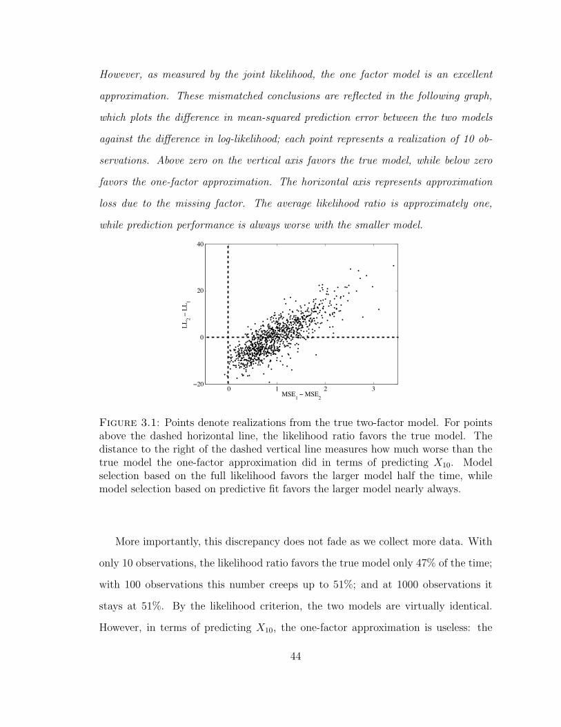
However, as measured by the joint likelihood, the one factor model is an excellent
approximation. These mismatched conclusions are reflected in the following graph,
which plots the difference in mean-squared prediction error between the two models
against the difference in log-likelihood; each point represents a realization of 10 ob-
servations. Above zero on the vertical axis favors the true model, while below zero
favors the one-factor approximation. The horizontal axis represents approximation
loss due to the missing factor. The average likelihood ratio is approximately one,
while prediction performance is always worse with the smaller model.
0 1 2 3−20
0
20
40
MSE1 − MSE2
LL2 −
LL 1
Student Version of MATLAB
Figure 3.1: Points denote realizations from the true two-factor model. For pointsabove the dashed horizontal line, the likelihood ratio favors the true model. Thedistance to the right of the dashed vertical line measures how much worse than thetrue model the one-factor approximation did in terms of predicting X10. Modelselection based on the full likelihood favors the larger model half the time, whilemodel selection based on predictive fit favors the larger model nearly always.
More importantly, this discrepancy does not fade as we collect more data. With
only 10 observations, the likelihood ratio favors the true model only 47% of the time;
with 100 observations this number creeps up to 51%; and at 1000 observations it
stays at 51%. By the likelihood criterion, the two models are virtually identical.
However, in terms of predicting X10, the one-factor approximation is useless: the
44
conditional and marginal variances are virtually identical.
Thus we see that relying on a prior distribution to correctly chose between a one-
versus two-factor model is a difficult task: the prior would have to be strong enough
to overwhelm more than a thousand observations’ worth of evidence which favor the
wrong model about half the time.
It may be instructive for some readers to understand this phenomenon from a
matrix decomposition point of view, by defining m to be the optimal value of the
The conditional regression parameters now borrow information from the marginal
distribution via the prior – we have centered the regression at the pure factor model.
47
However, the data may steer us away from this assumption. By decoupling the pre-
dictor distribution from the conditional distribution, prior specification on the poten-
tially ultra-high-dimensional predictor space does not affect our lower-dimensional
regression in counterproductive ways. At the same time, the hierarchical prior on
the regression parameters facilitates the borrowing of information that is necessary
in the p " n setting.
3.3.2 A conditional distribution view
Note that the prior on V , marginalizing over θ, is
V | B,Ψ Np0,BBt Ψq Np0,Σxq. (3.14)
Because β V Σ1X ,
covpβq Σ1X ΣXΣ1
X
Σ1X .
(3.15)
In other words, the partial factor model is a special case of the following hierarchical
model
Xi | ΣX Np0,ΣXq
Yi | Xi, β, σ2 NpX t
iβ, σ2q
β | ΣX , τ, σ2 Np0, τ1σ2Σ1
X q
(3.16)
where ΣX is restricted to have k-factor form. Note that conditional on ΣX this is
simply a conjugate Normal-Inverse-Gamma prior on the regression parameters:
β | σ2, S0 Np0, σ2S0q
σ2 IGpa, bq,(3.17)
with S0 τ1Σ1X . This observation permits easy comparison to two other common
linear regression priors. Taking the prior covariance matrix to be S0 τ1I gives
48
the well-known ridge estimator:
β Epβ | Y,Xq pXX t τ Ipq1XX tβ, (3.18)
where β is the (generalized) least-squares estimator
β pXX tq:XY
(where M : denotes the Moore-Penrose pseudo-inverse (Golub and Van Loan, 1996)
of M). Similarly, Zellner’s g-prior (Zellner, 1986; Liang et al., 2008) takes S0
g1pXX tq: yielding the estimator
β Epβ | Y,Xq p1 gq1β. (3.19)
To appreciate the benefit of using (3.16), consider the usual rationale behind
the ridge regression prior versus that of the g-prior. It is straightforward to show
that the ridge estimator downweights the contribution of the directions in (observed)
predictor space with lower sample variance, from which one may argue that (Hastie
et al., 2001):
Ridge regression protects against the potentially high variance of gradi-
ents estimated in the short directions. The implicit assumption is that
the response will tend to vary most in the directions of high variance in
the inputs.
The g-prior, by contrast, shrinks β more in directions of high sample variance in
the predictor space a priori, which has the net effect of shrinking the orthogonal
directions of the design space equally regardless of whether the directions are long or
short. This reflects the substantive belief that higher variance directions in predictor
space need not influence the response variable more than the directions of lower
variance.
49
However, this story conflates the observed design space with the pattern of
stochastic covariation characterizing the random predictor variable. It would be
more desirable to realize the benefit of regularizing estimates in directions of low
sample variance, while not over-regularizing regions of predictor space with weak
stochastic covariance structure. Teasing apart these two aspects of the problem can
be done by conditioning on X and ΣX covpXq separately, exactly as (3.16) does.
We may observe this teasing-apart effect directly from the form of the estimator
under (3.16). Assuming for simplicity that λ σ2 1, and let ΣX n1XX t and
V n1XY . Then
Epβ | Y,X,ΣXq pIp nΣ1x ΣXq
1pΣ1X V0 nΣ1
X V q, (3.20)
β0 Σ1X V0, (3.21)
where V0 is chosen a priori and determines the prior mean of the regression coeffi-
cients. Because ΣX and ΣX are never identical, we still get shrinkage in different
directions, thus combatting the “high variance of gradients estimated in short direc-
tions” while not having to assume that any direction in predictor space is more or
less important a priori.
In this light, we see that ridge regression is motivated by a mathematical fact
about regularization, while the g-prior is motivated by a substantive belief regarding
the influence of the predictor variables on the response (namely, symmetry). The
partial factor model can be understood as using X to learn about ΣX and then using
this information when trying to learn β.
Moreover, Zellner’s g-prior may be interpreted as a crude approximation to this
idea – rather than as a misguided regularization tool that shrinks the impact of
reliably measured covariates more than unreliable ones. The crucial distinction is
whether or not the predictors are taken to be fixed or stochastic. For example,
Maruyama and George (2010) advocate “more shrinkage on higher variance esti-
50
mates” and construct a prior on β which involves X, much like the g-prior, but which
amplifies the effect of ridge regression in that it results in more shrinkage in observed
directions of low sample variance. However, in the case of stochastic predictors, one
must distinguish between XX tn and ΣX , as we have seen in (3.20). The partial
factor model, which centers the conditional regression at a low-dimensional factor
model, actually recovers the g-prior-like expression (3.16). However, the k-factor
structure imposed on ΣX by the partial factor model provides a much improved es-
timator of ΣX over the naive sample covariance estimate that appears in the g-prior.
It is further instructive to consider the case where ΣX is given. Here, the difference
between (3.16) and ridge regression amounts to placing an independent prior on the
regression coefficients associated with the de-correlated predictors as opposed to
those corresponding to the original – possibly correlated – predictors. To see the
equivalence, let X pLtq1X, where LtL ΣX is the Cholesky decomposition of
the covariance matrix so that XY
Np0, Σq,
Σ
Ip αt
α ω
.
(3.22)
Then an independent prior on this regression pα | σ2, τq Np0, σ2τ1Ipq implies
pβ | ΣX , τ, σ2q Np0, σ2τ1Σ1
X q
as in (3.16) above.
This simple observation raises interesting questions about the role of “sparsity”
in linear regression models with stochastic predictors. Indeed, believing it plausible
that some of the regression coefficients are identically zero is incompatible with the
assumption that the same is true of the coefficients in the de-correlated predictor
space (for arbitrary covariances).
51
3.3.3 Efficient approximation
Sampling from the posterior distribution of the partial factor model may be achieved
via standard Markov chain Monte Carlo methods. In particular, a Gibbs sam-
pler for the ordinary factor model provides an excellent proposal distribution for
a Metropolis-Hastings update for many of the parameters. This approach provides
measures of posterior uncertainty over all parameters, up to Monte Carlo error. This
approach is slow, however, owing to the need to compute the determinant of a p-
dimensional matrix in computing the acceptance ratio. For the purpose of prediction,
the following approximation, which we call partial factor regression, proves useful.
Partial factor regression applies ridge regression to an augmented design matrix
with elements
Zi rfi ris
ri pXi BfiqΨ 1
2
(3.23)
mimicking the expression in (3.11). Two regularization parameters, τf and τr, are
then selected by cross-validation, corresponding to the respective regression coeffi-
cients on the latent factors and the residuals; these are analogous to q and w in
(3.13). Point estimates are obtained for Zi as the posterior mean of (3.3) using a
Gibbs sampling implementation. Partial factor ridge regression may be written as
Yi | Zi, γ, σ2 NpZt
iγ, σ2q,
γ | τf , τr Np0, σ2S0q,
S0
τ1f Ik 0
0 τ1r Ip
,
Zi EpZiq,
(3.24)
where the expectation in the last line is taken over the posterior πpB,Ψ, fi | X1:nq
derived from model (3.3).
52
This approach ignores the impact of Y on learning these parameters under the
partial factor model; however, this contribution should be minor in cases like those
considered in Section 3.2.2, turning a model flaw in the factor modeling context into a
computational shortcut in the partial factor setting. This step of the procedure may
be done ahead of time and may use as much marginal predictor data as is available,
to better estimate ΣX . Aside from this preprocessing, the model fitting is exactly
ridge regression using the augmented design matrix.
Moreover, this expression of the partial factor idea makes transparent where gains
may be achieved over other methods – by decomposing the regularization component
into two separate pieces, one concerned with the marginal stochastic structure of the
predictors and the other dealing directly with the conditional regression model.
Viewed from this perspective, the partial factor model is an instantiation of the
manifold regularization approach of Belkin et al. (2006), but motivated by an under-
lying generative model; τf is the “intrinsic” penalty parameter and τr is an additional
“ambient” penalty parameter. The key insight underlying the partial factor model is
precisely that these two components may be decoupled, even in the simple venerable
linear model.
3.4 Performance comparisons
3.4.1 Simulation study
This section considers the improvement the partial factor model can bring over stan-
dard Bayesian alternatives: the conjugate linear model with an independent “ridge
prior” (with unknown ridge parameter) and the Bayesian factor regression model.
We observe via simulation studies that the partial factor model protects against the
case where the response loads on a comparatively weak factor. The partial factor
model is most frequently the best performing model (modally optimal), and it is also
the best model on average (mean optimal) in unfavorable low signal-to-noise regimes
53
and nearly so in the high signal-to-noise case. In summary, the partial factor model
predicts nearly as well as the conjugate linear model and factor models when those
models perform well, but it does much better than those models in cases where they
do poorly. This profile is consistent with results of the multiple-shrinkage principal
component regression model of George and Oman (1996), which has a similar moti-
vation – seeking to mimic principal component regression but to protect against the
least-eigenvalue scenario – but is not derived from a joint sampling model.
For this simulation study, let p 80 and n 50. Of the 50 observations, 35
observations are labeled with a corresponding Y value. Across 150 data sets, the
remaining 15 unlabeled values were predicted using the posterior mean imputed
value.
The data were generated according to the following recipe.
1. Draw k Uniformpt1, , n 1uq.
2. Generate a matrix A of size p k with independent standard Normal random
variables.
3. Generate a k k diagonal matrix D with elements drawn from a half-Cauchy
distribution.
4. Set the true loadings matrix B AD‖AD‖ where ‖‖ denotes the Frobenius
norm.
5. Draw the elements of Ψ independently as folded-t random variables with 5
degrees of freedom and scale parameter 0.1.
6. Lastly, draw θ by first drawing a folded-t scale parameter and then drawing a
mean zero random variable with corresponding scale.
54
We consider two scenarios. In the first, the elements of θ and D are ordered so
that the highest absolute value of D corresponds to the highest absolute value of θ,
the second highest corresponds to the second highest, etc. This is a favorable case for
the assumptions of ridge regression and factor models in that the response depends
most on the directions of highest variability in predictor space. For the second case
the elements of θ and D are arranged in reverse order; the smallest absolute value of θ
is associated with the largest absolute value of D. In this case the highly informative
directions in predictor space are least informative of the response in terms of variation
explained.
Table 3.1: PFR: Partial factor regression. NIG: conjugate prior linear regression.BFR: Bayesian factor regression. Both the factor model and the partial factor modelselected k a priori by looking at the singular values of design matrix, so that the topk singular vectors account for 90% of the observed variance.
Case One.Method % best mean relative error scaled MSE
PFR 36 .37 1.06NIG 19 .48 1BFR 29 7.27 1.89
Case Two.Method
PFR 43 .27 1NIG 17 .45 1.04BFR 30 3.87 1.32
To compare the average behavior of these methods on a wide range of data we
may look at the paired hold out error on each of the sets. We record the frequency
that each method was the best performing method, the average relative error (the
average of the ratio of the squared error of the method to the minimum squared error
over the three methods), and also the overall mean square error. The first measure
records how often we should expect a method to be the best method to use on a
randomly selected data set, so that higher numbers are better. The second column
55
reflects how far off, on average, a given method performs relative to the best method
for a given data set; smaller numbers are better. The final column gives the average
error relative to the best overall method; numbers nearer to one are better.
We observe that in the favorable setting the pure factor model is quite often the
best model of the four, as shown in the first column. However, we notice also that
when it is not the best, it performs, on average, much worse than the best method,
as shown in the second column. This is the impact of the bias. Next, we note that
while ridge regression moderately outperforms the partial factor model in terms of
overall mean squared error, we see that on average partial factor regression is closer
to the best performing model. Relatedly, it is the partial factor model that is most
often the best model.
In the unfavorable setting, results unambiguously favor the partial factor model.
In this setting, as expected, the partial factor model outperforms ridge regression by
all three measures. Again, the pure factor model is crippled by its too-strong bias.
3.4.2 Real data examples
In this section, we extend our comparisons to additional methods and to the case
of real data. We compare partial factor regression to four other methods: princi-
pal component regression (PCR), partial least squares (PLS), least-angle regression
(Efron et al., 2004) (LARS), and ridge regression (RR). We observe the same pattern
of robust prediction performance as in the simulation study. Partial factor regression
shows itself to be the best or nearly the best among the methods considered in terms
of out-of-sample mean squared prediction error.
Five real data sets in the p ¡ n regime are analyzed; the data are available
from the R packages pls (Mevik and Wehrens, 2007), chemometrics (Varmuza and
Filzmoser, 2009), and mixOmics (Cao et al., 2009).
nutrimouse: the hepatic fatty-acid concentrations of 40 mice are re-
56
gressed upon the expression of 120 liver cell genes.
cereal: the starch content of 15 cereals is regressed upon 145 different
wavelengths of NIR spectra.
yarn: the yarn density of 28 polyethylene terephthalate (PET) yarns is
regressed upon 268 wavelenths of NIR spectra.
gasoline: the octane numbers of 60 gasoline samples are regressed upon
401 wavelengths of NIR spectra.
multidrug: an ATP-binding cassette transporter (ABC3A) is regressed
upon the the activity of 853 drugs for 60 different human cell lines.
To test the methods, each of the data sets is split into training and test samples,
with 75% of the observations used for training. Each model is then fit using the
training data, with tuning parameters chosen by ten-fold cross validation on the
training data. Out-of-sample predictive performance on the holdout data is measured
by sum of squared prediction error (SSE).
Table 3.2: PFR: partial factor regression. RR: ridge regression. PLS: partial leastsquares. LARS: least angle regression. PCR: principal component regression. Per-centages shown are amount worse than the best method, reported in bold type.
Average out-of-sample errorData set n p PFR RR PLS LARS PCR
As shown in table 3.2, the partial factor model outperforms all models on three of
the five data sets. In the other two data sets, the nutrimouse and multidrug exam-
ples, the factor structure was weak, requiring k n to account for the variation in
the predictor space. In these cases, the extra variance of learning two tuning param-
eters does not pay dividends and ridge regression narrowly comes out on top. Even
57
so, partial factor regression is never much worse than the best. In cases where the
predictor space can be described well by low-dimensional (linear) structure, partial
factor regression outperforms methods such as principal component regression, which
require that this same structure account for all of the variability in the response.
Note that these data were selected because they are publicly available and fall
within the p ¡ n regime that is most germane to our comparisons.
3.5 Variable selection and subspace dimension estimation
3.5.1 Sparsity priors for variable selection
In this and the next section, it is convenient to work with a reparametrized form of
the partial factor model, defining
Λ pV θBtqΨ 12 (3.25)
and using the equivalent independent prior
Λ Np0, w1Ipq. (3.26)
Note that Λ 0 represents a pure factor model, and that this prior is independent
of the other parameters. The revised expression for our (latent) regression becomes
Y θf ΛΨ 12 pX Bfq ε, ε Np0, σ2q. (3.27)
If λj 0, predictor Xj appears in the regression of Y only via its dependence on
the latent factors. Further, if we assume that θ is not identically zero so that Y has
some relation to the latent factors, then we see that if bj 0 (so that dimension j
does not load on any of the factors) and λj 0, then βj 0 necessarily. That is,
if Xj is not related to any of the latent factors governing the predictor covariance
and additionally is not idiosyncratically correlated with Y via λj, then Xj does not
feature in our regression. The reverse need not hold; the net effect of Xj on Y
58
can appear insignificant if Xj has a direct effect on the response, but is positively
correlated with variables having the opposite effect.
Partial factor regression helps distinguish between these two scenarios, because
the framework permits sparsity to be incorporated in each of three separate places
in the model:
1. Does variable Xj load on latent factor fg (bjg 0 versus bjg 0 )?
2. Does Y depend on the residual of element Xj; is Xj important for predicting
Y above and beyond the impact of the latent factors (λj 0 versus λj 0)?
3. Does Y depend on latent factor fg (θg 0 versus θg 0)?
This decomposition avoids the unsatisfactory choice of having to decide which of
two variables should be in a model if they are very highly correlated with one another
and associated with the response. Rather it allows one to consider the common effect
of two such variables in the form of a latent factor, and then to consider separately if
both or neither should enter into the model residually via the parameter Λ. Earlier
work has keyed onto the idea that covariance regularization is useful for variable
selection problems (Jeng and Daye, 2011); here these intuitive decompositions follow
directly from the generative structure of the partial factor model.
Such a variable selection framework may be implemented with the usual variable
selection point-mass priors on θ, Λ and B. Previous work incorporated such priors
for the elements of B (Carvalho et al., 2008). Alternatively, shrinkage priors and
thresholding may be used to achieve a similar effect.
3.5.2 Subspace dimension estimation
In the case of multivariate Normal random variables, a factor decomposition of the
covariance matrix, in combination with point mass priors as described above, admits
a ready characterization of the dimension reduction subspace (Cook, 2007; Cook
59
and Forzani, 2008; Wu et al., 2010) with respect to the response Y . A dimension
reduction subspace is the span of a projection of the predictors which is sufficient to
characterize the conditional distribution of the response.
In the factor model setting, we can calculate the dimension of this subspace as
follows (Mao et al., 2010). Let θY denote the nonzero elements of θ in the partial
factor parameterization. Denote by BY the corresponding columns of B and likewise
let BX denote the remaining columns. Then, if Λ 0, the conditional distribution
of Y given X can be characterized purely in terms of
EpY | Xq θBtpBBt Ψq1X
θY BtT pBY Bt
Y BXBtx Ψq1X
θY BtY pBY Bt
Y ∆q1X
θY rIBtY ∆1BY pIBt
Y ∆1BY q1qsBt
Y ∆1X,
(3.28)
where ∆ BXBtX Ψ, showing that X enters this distribution only via Bt
X∆1X.
Thus, the rank of BY is the dimension of the reduced subspace, as long as we have
a pure factor model. We have already seen, however, that while a covariance matrix
may be relatively well approximated by a small number of factors, these factors
alone may not span the dimension reduction subspace, so that θ is estimated to be
approximately zero and σ2 is biased upward.
Accordingly, we estimate PrpΛ 0 | X, Y q, the posterior probability that the
sufficient subspace is less than k rankpBq. Further, by monitoring the number of
nonzero elements of θ in our sampling chain, we can estimate the sufficient dimension,
conditional on it being less than k. This approach may be thought of as partitioning
our prior hypotheses as
Hj : rankpBY q j, j P t1, . . . , ku
H0 : rankpBY q ¡ k.(3.29)
The prior probabilities assigned to these hypotheses are induced via priors on k and
60
Λ; grouping many individual hypotheses into the aggregate H0 permits easier control
of the contribution of the prior, which can be critical to inference when p " n.
3.6 Conclusions
In the p " n setting, inference and prediction may sometimes be improved by making
structural simplifications to the statistical model. In a Bayesian framework this can
be accomplished by positing lower-dimensional latent variables which govern the joint
distribution between predictors and the response variable. An inherent downside
to this approach is that it requires specifying a high-dimensional joint sampling
distribution and the associated priors. Due to the high dimensionality this task is
difficult, particularly with respect to appropriately modulating the implied degree of
regularization of any given conditional regression.
The partial factor model addresses this difficulty by reparametrizing the joint
sampling model using a compositional representation, allowing the conditional re-
gression to be handled independently of the marginal predictor distribution. Specif-
ically, this formulation of the joint distribution realizes borrowing of information via
a hierarchical prior rather than through a fixed structure imposed upon the joint
distribution.
Here we have examined the simplified setting of a joint Normal distribution. How-
ever, the idea of utilizing a compositional representation in conjunction with a hier-
archical prior can be profitably extended to many joint distributions. In particular,
one may specify the joint distribution directly, building in borrowing of information
by design. For example, the form of the conditional moment for the partial factor
model suggests the following nonlinear generalization:
EpY | f,Xq gpfq hpX EpX | fqq, (3.30)
where perhaps g and h denote smooth functions to be inferred from the data. Here,
61
the smoothness assumptions for g and h could be different; specifically the prior on
h could be conditioned on properties of g. More generally, the partial factor model
is a special case of models of the form:
fpY,X | Θq fpX | θXqfpY | X, θX , θY q (3.31)
πpΘq πpθY | θXqπpθXq, (3.32)
where Θ tθX , θY u generically denotes parameters governing the joint distribution.
In the partial factor model θX tB, F,Ψu and θY tσ2, V u. The conditional model
depends on both θX and θY , but the presence of θY in the model leads to a more
flexible regression, while the hierarchical prior (4.21) still borrows information from
the predictor variables via θX .
Such models alleviate the burden of having to get the high-dimensional distribu-
tion just right in all of its many details. As such, it represents a robust method for
fashioning data-driven prior distributions for regression models.
62
4
A Latent Variable Model for Testing CognitiveHierarchy Theories of Beauty Contest Games
In this chapter, the interpretational challenges of latent variable mixture models are
considered in the context of an application to the exciting new field of behavioral
game theory. The ultimate goal is to assess whether or not a popular psychological
theory of strategic reasoning is being adopted by real subjects. The primary challenge
is that people are notoriously bad at self-reporting mental activities (Payne et al.,
1993), rendering the relevant state variables inherently unobservable. This chapter
is intended both as an introduction to the world of behavioral game theory for the
statistician and as an explicitly statistical perspective on a well-known example for
the behavioral economist. As such, it does not aspire to summarize the entire field
or provide a comprehensive bibliography; interested readers would do well to start
with Camerer (2003) and references therein. The approach here is rather to look in
detail at one very simple game and to develop from scratch a model that admits a
rigorous statistical analysis.
Broadly speaking, behavioral game theorists investigate the gap between how real
63
people strategize (or fail to do so) and the way the formal mathematics suggests they
ought to; specifically, they attempt to bridge this gap with psychological science. This
pairing offers psychology a certain measure of precision inherited from game theory,
where behavior is restricted to a limited variety of moves, and offers game theory
the potential to extend its reach beyond the confines of pure formalism. A successful
behavioral game theory model should formalize the strategic reasoning of players
in a way that 1.) satisfies stipulated rationality constraints, and simultaneously
2.) provides a good description of observed game play. In practice, the model is
constructed to satisfy the first condition so that if the second condition obtains, one
can analyze the model as if the first condition were met. In general, one cannot prove
that the observed behavior was generated in the rational way dictated by the model,
but by augmenting our data with theoretical assumptions one can draw interesting
– though contingent – conclusions.
This chapter advances both the rational constraint modeling and the empiri-
cal testing aspects of one specific game. First, a new flexible Bayesian model is
constructed which encodes the structural game-theoretic assumptions while vastly
generalizing models from the previous literature (Crawford, 2007; Camerer et al.,
2004). For the game considered here – called the α-beauty contest – the necessary
model takes the form of a finite mixture of Beta distributions with special inequal-
ity conditions imposed on the means of the mixture components. Additionally, a
graphical prior elicitation procedure is developed. Second, structural invariants of
the likelihood function across different experimental conditions are identified, which
facilitates more powerful hypothesis tests using a posterior holdout log likelihood
score, (similar to a Bayes factor, but less sensitive to prior specification). Newly
collected data provides evidence that the simpler models of the previous literature
are not well supported by the data.
64
4.1 Review of cognitive hierarchy theories of beauty contest games
Experiments consistently demonstrate that people do not always strategize the way
that mathematical game theory says they ought to (Camerer, 2003). Cognitive
hierarchy (CH) theories of strategic reasoning elegantly account for this fact by taking
into consideration players’ beliefs about how their opponents will play (Crawford,
2007). Contrary to the Nash equilibrium of a game, which one arrives at by assuming
that all players are capable of reasoning their way to the equilibrium solution and
that all players assume as much about one another (Bosch-Domenech et al., 2002;
Stahl and Wilson, 1995), CH models posit that people do not reason all the way to
equilibrium because doing so simply requires too much effort and/or ability1 (Costa-
Gomes and Crawford, 2006; Crawford, 2007; Stahl and Wilson, 1994, 1995; Nagel,
1995).
CH models propose instead that there exists a hierarchy of player types, corre-
sponding to the different numbers of steps that players reason ahead in a game. Some
people – call them level-0 players – simply play at random. Level-1 thinkers reason
that people play randomly in this way, and they play the optimal strategy given
this assumption. Level-2 players assume that some fraction of players are using a
random strategy and that the remainder of players are level-1 players, and they play
the optimal strategy given this assumption, and so on. CH models often generate
better predictions of behavior than Nash equilibrium. While this marks CH models
as better descriptions of empirical game play, here we attempt to determine whether
such descriptions are in fact accurate ones. That is, we attempt to assess the sta-
tistical evidence for the hypothesis that people are playing according to a cognitive
hierarchy.
1 Indeed, the sort of reasoning required to arrive at the equilibrium solution is formal mathematicalinduction, a process with which people are known to struggle (Newell and Simon, 1972; Johnsonet al., 2002).
65
Although CH models have been developed for a wide variety of games, we base
our analysis on the α-beauty contest game (Moulin, 1986; Nagel, 1995), owing to its
simplicity and high profile in the existing literature. On the one hand, this narrow
focus on one game is inherently limiting. On the other hand, this very simple game is
the quintessential CH model, because “the sharpest evidence on iterated dominance
comes from α-beauty contest games (Camerer, 2003)”. Our purpose is to critically
assess that evidence.
We do this by comparing the CH model to an appropriate non-CH alternative,
an approach that is relatively uncommon in the literature, a notable exception being
Stahl and Wilson (1995). We share these authors’ conviction that “[f]or the pur-
poses of hypothesis testing of alternative theories, it is necessary to construct an
encompassing econometric model.” The majority of our paper is devoted to devel-
oping just such an encompassing model for the α-beauty contest, which we call the
semiparametric cognitive hierarchy (SPCH) model. This model nests most published
CH models as special cases.
We collect new beauty contest data from an experiment designed to highlight the
signature patterns of CH play. Analyzing this data, we find that our flexible SPCH
model convincingly outperforms earlier variants in the literature (called the CH-
Poisson model and the level-k model, to be defined) in terms of predicting player
behavior. Moreover, these earlier models do worse than a non-CH null model, in
which players’ behavior is not constrained to reflect a cognitive hierarchy at all.
The newly introduced SPCH model does better than this non-CH null model. More
plainly, we find no evidence in support of the specific earlier CH variants, but do find
compelling evidence of behavior consistent with some cognitive hierarchy model.
In the following section we briefly review the α-beauty contest and lay out the
previously proposed CH-Poisson and level-k models (Camerer et al., 2004; Crawford,
2007).
66
4.1.1 Beauty contest games
The goal of each player of the α-beauty contest2 (Moulin, 1986; Nagel, 1995) is to
report a number b – referred to here as a bid3 – that is as close as possible to α times
the whole group’s average bid. Bids are restricted to lie within some fixed interval
pL,Uq. Formally we can say that for a beauty contest played among N players,
player i has a payoff defined by
uipbq M dpbi αbq (4.1)
where dpq is some distance metric, b denotes the realized N -vector of bids, M
dpU Lq, and b N1°Nj0 bj. For example, a beauty contest on an interval from
0 to 100 could have a payoff of $p100 |bi αb|q.
The Nash equilibrium for α P p0, 1q is 0. Everyone in the group is trying to
undercut everyone else’s bid by the fraction α, driving the equilibrium strategy to
zero. Nonetheless, experiments consistently reveal that many, if not most, people do
not play the zero strategy.
The beauty contest game has many desirable properties from an analyst’s point
of view, two of which we note here. First, it is a symmetric game, meaning that all
players have the same payoff function. Second, for large N ,
dpbi αbq dpbi αbiq 0 (4.2)
2 Beauty contest games are so-called after a quote by Keynes (1936), first cited in this context byNagel (1995): “professional investment may be likened to those newspaper competitions in whichthe competitors have to pick out the six prettiest faces from a hundred photographs, the price beingawarded to the competitor whose choice most nearly corresponds to the average preferences of thecompetitors as a whole . . . It is not the case of choosing those which, to the best of one’s judgment,are really the prettiest, nor even those which average opinion genuinely thinks the prettiest. Wehave reached the third degree where we devote our intelligences to anticipating what average opinionexpects average opinion to be. And there are some, I believe, who practise the fourth, fifth, andhigher degrees.”
3 We introduce this term as an intuitive one for the non-specialist; it is not intended to evoke anauction setting. If preferred, the b could be read as “behavior”.
67
where
bi Nb biN 1
(4.3)
is the mean of the other N 1 observations, so that payoff maximization effectively
depends only on the average bid of the other players, irrespective of one’s own bid.
This follows because the boundedness of the bids entails that the contribution of
any one bid to the overall mean grows like 1N . From this perspective, it becomes
natural to ask if the observed non-Nash play in the α-beauty game is a result of
rational agents acting on the conviction that their opponents are acting irrationally
so that αbi 0. If a given player does not trust that his opponents can reason
their way to the Nash equilibrium strategy, then the Nash equilibrium solution is no
longer optimal or rational for that player.
This fact suggests that characterizing players’ beliefs about the strategies others
play may be one route to accurately characterizing actual bidding behavior. Such an
approach poses two questions. First, can we come up with plausible restrictions on
the belief distributions so as to constrain the possible behavior that would qualify
as rational? Second, how might we test if those restrictions are actually obeyed in
Camerer et al., 2004) are a natural candidate to address the first question and we
describe these models in the next section. Then, the remainder of the paper takes
up the second question.
4.1.2 Cognitive hierarchies
A CH model is built upon several prima facie reasonable premises:
1. Players are distributed among a discrete collection of strategy classes defined
by the number of steps ahead in the game players will reckon when formulating
their strategies.
68
2. Players have strategy-class-specific beliefs about the relative proportion of play-
ers in strategy classes lower than themselves.
3. Players assume that they are thinking at least one step ahead of any other
player.
4. Players will best respond in the sense of maximizing expected payoff conditional
on their beliefs.
The first and second conditions mean that an agent’s strategic beliefs cannot be
wholly idiosyncratic. Condition three is a convenient and plausible restriction, which
can be thought of as an “arrogance” assumption. The final condition is the usual
payoff maximization assumption.
These assumptions alone leave too many degrees of freedom in that both the dis-
tribution of the players across the various strategy classes and also the strategy-class-
specific belief distributions remain undetermined. Even if all these various distribu-
tions took simple parametric forms, the model would pose estimability difficulties,
with N latent class memberships and up to N class-specific belief distributions free
to vary.
The CH-Poisson model
Camerer et al. (2004) handle the indeterminacy of CH models by fiat, adding three
additional – and quite restrictive – assumptions to those above:
P5. Players are distributed among strategy classes via a Poisson(τ) distribution.
P6. Players have accurate beliefs about the relative proportions of players in strat-
egy classes lower than themselves.
P7. Players in the lowest strategy class issue bids uniformly at random over the
allowed interval.
69
Taken together, these additional assumptions define game play for any strategy
class: players will maximize their expected payoffs with respect to their class-specific
belief distribution on strategy classes, given as gkphq fτ phq°k1l1 fτ plq, where
f is the probability mass function of the Poisson distribution. A step-k player’s
best response can then be found iteratively by computing the best response for all
strategy classes below k. Model fitting is thereby reduced to the estimation of a single
parameter τ . Model assessment or evaluation can then be conducted according to
some criterion, conditional on this parameter estimate.
The first of these additional assumptions, the parametric assumption, is less
restrictive than the other two. Condition P6 is easily the most restrictive because it
implies that the bidding behavior of all the strategy classes is coordinated purely by
the true underlying distribution. This condition would be equally constrictive even if
the underlying distribution were not a single-parameter distribution like the Poisson.
Condition P7 puts an upper bound on where any (non-level-0) strategy class can bid
by fixing the mean bid the level-0 players.
Thus, the CH-Poisson model consists of a discrete component, constituting a
countably infinite collection of bids, the values of which are determined by a sin-
gle parameter, τ , and a continuous component, which is the uniform distribution
from which the bids of level-0 players are assumed to be drawn. On the face of
it, the actual data4 (Ho et al., 1998) exhibit many properties that would seem
to rule out the CH-Poisson model, including a lack of many identical bids corre-
sponding to the discrete component of the CH-Poisson and also approximately equal
number of bids below 1/2 as above. This misfit may be formalized somewhat by
comparing the sample mean, the estimator for τ used in Camerer et al. (2004), to
τ log p2N1°Nj1 1pbj ¡ 12qq, a consistent estimator based explicitly on count-
4 We thank Teck Ho for making these data available to us. The data we have shown here aggregateseven groups of seven players each, all playing with the same α 0.7.
70
Frequency of bids, ! = 0.7
0.0 0.2 0.4 0.6 0.8 1.0
02468
Figure 4.1: Strategic play is not overwhelmingly apparent from the raw data,which appears roughly uniform. We have rescaled here to the unit interval (as wewill throughout).
ing the known level-0 players. For the data shown this degree of sophistication is
unnecessary, as the sample mean is an unattainable (under CH-Poisson) 0.52. That
is, the population mean of a CH-Poisson model with uniform random level-0 players
can never be greater than 1/2 for any value of τ , so that a sample mean of 0.52 yields
an undefined estimate.
Level-k model
The level-k model, as decribed in Crawford and Iriberri (2007), is a CH model
in which every player assumes that all the other players are in the strategy class
immediately below them. That is, it modifies P5-P7 as follows:
LK5. Players are distributed among K strategy classes via a multinomial distribution
with probability weights π.
LK6. Players believe that all of their opponents reason exactly one step less than
they do.
LK7. Players in the lowest strategy class issue bids uniformly at random over the
allowed interval.
71
Notice that LK7 and P7 are identical, that LK5 is less restrictive than P5, but
most importantly that these assumptions, like P5-P7, uniquely define optimal play
across all strategy classes. One of the upshots of our analysis is the ability to deter-
mine which set of assumptions, if any, is a good match to observed bidding behavior.
4.2 Building a semiparametric model for beauty contest data
Our aim is to develop a model that affords great flexibility in the range of beliefs
it permits a rational player to hold, while still admitting statistical analysis. More-
over, it should nest the more restrictive assumptions of the CH-Poisson and level-k
formulations to facilitate model comparison. In the following subsections we develop
these properties of our generalized CH model from the ground up. As a CH model,
our model will retain conditions 1-4 from above. We will replace conditions P5-P7
of the CH-Poisson and LK5-LK7 of the level-k model with less rigid analogues.
4.2.1 Monotonically decreasing target bids
Rather than explicitly specifying each strategy class’s belief distributions, we adopt
a less strict characterization which only specifies how the various strategy classes bid
relative to one another.
It will be valuable from here out to distinguish carefully between three related,
but distinct quantities. First we denote by Tk the target bid of a strategy class k
player – α times the value that such a player expects will be the mean play of his
opponents. Secondly, we will denote by bi the observed bid of the ith player. Lastly,
we will denote by bi the utility-maximizing bid for agent i.
Thus equipped, we can express our first restriction as
Tk Tk1 whenever k ¡ k1. (4.4)
In words, higher step-ahead thinkers are required to have lower target bids. Under-
72
standing this requirement is aided by some notation. Recall that for relatively large
N (tens or hundreds), we can express Tk as
Tk αk1
j1
gkpjqTkpjq (4.5)
where Tkpjq is a level-k player’s belief as to the target value of a level j k player.
This expression makes clear the impossibility of formally distinguishing between
a given player type’s belief distribution, gkpjq, and his beliefs about the other player’s
beliefs, from which Tkpjq is derived. But if we make an additional assumption that
players of strategy level k know gk1 for all k1 k (4.6)
we can further extend our analysis. At an intuitive level, the appeal of this assump-
tion is that it jibes with a strong conception of a cognitive hierarchy – not only do
some players reason more steps ahead than others, those players are also assumed to
have the capacity to project themselves into the strategic viewpoint of lower strategy
classes, though the reverse is not possible5.
This new assumption, along with the assumption that all players are conditionally
rational actors, entails that
Tkpjq Tj (4.7)
and we have the following recursive identity:
Tk αk1
j1
gkpjqTj, (4.8)
5 We might add that under some interpretations of the level-k model (Costa-Gomes et al., 2001), alevel-k player does not have any beliefs about the strategies of players lower than k1. Observed bidsalone cannot distinguish between this case and the case where players have beliefs about all players,but simply believe that there are no players lower than k1 in the population (gkpk1q 1). Thisis a special case of the unidentifiability of gpq and we do not address this point further. We stress,however, that if the bidding data alone does not support either model, the need to distinguishbetween the two is moot.
73
from which we can investigate what sorts of restrictions on the belief distributions
g are implied by the order restriction given in (4.4). A straightfoward calculation
shows
Tk1
Tk
α°kj0 gk1pjqTj
α°k1h0 gkphqTh
(4.9)
°k1j0 gk1pjqTj gk1pkqTk°k1
h0 gkphqTh(4.10)
p1 gk1pkqq
°k1j0
gk1pjqp1gk1pkqqTj gk1pkqTk
EkpT q(4.11)
p1 gk1pkqqEk1pTj | j kq
EkpT q αgk1pkq (4.12)
¤ 1. (4.13)
That is, dealing with (4.4) is equivalent to working with distributions g which satisfy
(4.12); this is restriction SP6. This expression is relatively easy to interpret, the
left-hand side being a convex combination of α and the ratio of the expectations
of the pk 1q-level and k-level player regarding what the opposition will bid. As
might be expected, the requirements on the belief distributions g take the form of a
moment constraint only, meaning that we obtain considerable variety in the shapes
of distributions permitted under (4.4).
Indeed, the CH-Poisson model and the level-k model both use distributions sat-
isfying (4.4). In the first case this follows becauseEk1pTj |j kq
EkpTjq 1 under the CH-
Poisson model so that we have
αgk1pkq ¤ gk1pkq
which is true whenever α ¤ 1. In the second case, gk1pkq 1 so that we find the
condition is again satisfied whenever α ¤ 1.
74
4.2.2 Incorporating error
As noted, empirical α-beauty data exhibit a greater variety of observed bids than the
CH-Poisson or level-k models would suggest. In particular, the degree of observed
heterogeneity points to additional sources besides the level-0 players. Because any
CH-model, as described so far, permits just one optimal bid per strategy class, we
find that, (excepting level-0 players), the number of unique plays we observe must
correspond to the number of strategy classes appearing in our sample. Underly-
ing this mathematical observation is the simple fact that any realistic CH model
should allow players to deviate to various degrees from their optimal target bid. The
observation that individuals will often bid distinct amounts in separate instances
of the α-beauty contest played some duration apart is strong motivating evidence
for building “jitter” into our CH model. Others that have taken this approach are
De Giorgi and Reimann (2008); Stahl and Wilson (1995); Haruvy et al. (2001) and
Bosch-Domenech et al. (2010).
4.2.3 Conditional rationality
Fortunately, incorporating optimization error can be done without violating condi-
tional rationality, subject to a few natural assumptions. First, we assume that each
agent’s bid comes from a class-specific distribution with class-specific mean given by
the target bid for that class, Tk, as previously defined. Secondly, we assume that the
payoff function uses squared distance, so that in (4.1) we have
dpq pq2. (4.14)
We now demonstrate how these two assumptions preserve conditional rationality for
each strategy class.
75
Let
B0 F0 EpB0q T0
B1 F1 EpB1q αT0 T1
B2 F2 EpB2q αrg2p0qT0 g2p1qT1s
...
Bk Fk EpBkq αk1
j0
gkpjqTj
be the random variables describing the bids of players from the various strategy
classes, and let γi be the indicator variable denoting strategy class membership of
the ith individual so that bipγiq denotes the observed bid of individual i subject to
being a level-γi player. Under the squared-error loss function we then have that the
optimal bid for player i if he knew exactly the bids of the other players is given as
bipγiq | b arg maxb
pb αbq2
arg maxb
pb αbiq2.
Using this approximation we can integrate over player i’s strategy-class-specific be-
liefs (given as gγi) and express the optimal play as
bipγiq arg maxb
Egγi
b α
¸mi
Bm
N 1
2 .
More suggestively we can note that°mi
BmN1
can be written as a sum of pN 1q in-
dependent and identically distributed draws from a distribution Gγi °k1j0 gγipjqFj
which has mean α1Tγi (as defined above). Applying a well-known result from de-
cision theory which states that the optimal solution under expected squared loss is
76
the mean, we see that Tγi is indeed conditionally optimal6 . That is,
bi pγiq Tγi
so that the cognitive hierarchy with optimization error still coheres as long as players
assume that everyone will play optimally in the mean. Notationally, it may be helpful
to think of the observed plays as
bipγiq Tγi εi
where Epεiq 0 for all γi.
To summarize, Tk is what a level-k player “intends” to play, which is his optimal
play subject to his beliefs about the other players given that they too intend to play
optimally; what he actually plays is bipkq, which can be thought of as an observation
of a random variable Bk Fk with EpBkq Tk.
Even though individuals play with random errors about their class-specific mean,
the mean structure itself is rational even with respect to this randomness in the bids.
4.2.4 Error distribution
So far we have defined a nonparametric analytical model for the cognitive hierar-
chy. Agents playing according to this model are conditionally rational, organized
hierarchically, free to hold flexible class-specific belief distributions, and free to make
mistakes in their utility maximization, so long as they get things right in expectation.
However, for testing purposes we are free to employ a flexible parametric model.
Specifically, we introduce a Beta error model and propose to learn about the latent
strategy classes using a conjugate Bayesian Dirichlet-Multinomial model. Notice
6 Note that once players are asked to accommodate uncertainty (in this case, from two sources– the uncertainty over strategy class membership and that due to bidding error) the exact formof distance used in the payoff function becomes important in calculating the optimal CH bid; inparticular, distinct nonlinear distance metrics will result in a distinct set of target bids.
77
that this entails that the underlying distribution of strategy classes will be a discrete
distribution of K strategy classes, equivalent to LK5 (but different than P5).
The assumption of Beta errors is convenient and innocuous from a purely game-
theoretic perspective – none of the previous development hinged on particular fea-
tures of the belief distributions beyond the first moments. Statistically, this approach
entails that our inferences about model parameters are made conditional on our para-
metric assumptions, but we take this as a virtue rather than a vice. The Beta is
computationally tractable and contains the uniform distribution as a special case.
See also Bosch-Domenech et al. (2010) for the use of Beta distributed errors in the
context of beauty contest games.
4.3 Exploiting the exogeneity of α to infer strategy-class membership
The SPCH model has so far been described for a fixed value of α. Consistent with
prior literature, we take α to be functionally independent of the belief distributions
g, the vector of strategy class indicators γ, and also the bidding errors ε. This
exogeneity has two interesting consequences.
First, g not being a function of α implies immediately that Tkpαq is a decreasing
function of α for k ¡ 0. This fact suggests relaxing the assumption that the level-0
players have a constant bidding distribution across values of α (as in Camerer et al.
(2004) where these players draw their bids from a fixed uniform distribution). A
more flexible alternative is to let the level-0 players have target bids that follow
a nondecreasing function of α, which will become condition SP7. Others that have
investigated relaxing the uniform level-0 assumption include Haruvy and Stahl (2008)
and Ho et al. (1998). In this case,
Tkpαq ¤ Tkpα1q for all k and α α1 (4.15)
with no additional modifications necessary.
78
Second, γ not being a function of α implies that strategy-class membership is a
fixed attribute of a player that does not change from game to game. Accordingly,
having subjects bid without feedback for various values of α gives us multiple observa-
tions from which to infer class membership. Intuitively, observing bids over multiple
values of α permits us to discern if any observed clustering of bids is a result of CH
behavior by checking that those clusters evolve suitably with changing α (see figures
4.2 and 4.3). Formally, it yields the following factorization of the likelihood:
K
k1
πk
J¹j1
Betapbpαjq | ak,j, βk,jq
. (4.16)
Keep in mind that this factorization is in addition to the previously described order
conditions on the target bids, which enter the likelihood via aj and βj.
This factorization of the likelihood has important consequences for parameter es-
timation and model evaluation – two densities (for two α levels) that appear to match
the data when looked at individually could not, in some instances, have plausibly
come from a CH model if evaluated jointly across the two levels.
4.4 Putting the pieces together
To recap, we have in place of A5-A7 or LK5-LK7 the following restrictions:
SP5. Players are distributed among K strategy classes via a multinomial distribution
with probability weights π.
SP6. Players’ strategy-class-specific belief distributions gk must satisfy,
for all k and α:
p1 gk1pkqqEk1pTj | j kq
EkpT q αgk1pkq ¤ 1.
SP7. Target bids for level-0 players follow a nondecreasing function of α.
79
0.0 0.2 0.4 0.6 0.8 1.0
0.0 0.2 0.4 0.6 0.8 1.0
0
0 1
1
Figure 4.2: Lines connect players’ bids across games with differing levels of α.This plot illustrates valid CH play wherein individuals do not switch mixture com-ponent/strategy class across games.
0.0 0.2 0.4 0.6 0.8 1.0
0.0 0.2 0.4 0.6 0.8 1.0
0 1
0 1
Figure 4.3: Switching class across α, as shown here, is not permitted under a CHmodel.
Working with these three assumptions, we avoid having to specify or estimate the
belief distributions g. As a result, we are able to estimate target bids and strategy-
class membership probabilities that are consistent with a wide range of possible CH
models. While this setup cannot by itself distinguish finely between specific cases, it
represents a benchmark CH model for testing the assumptions of the CH framework
80
generically.
4.5 Data and analysis
Finally, we describe the new α-beauty contest data we have collected, all the formal
details of our model, as well as our analysis and conclusions. We begin by describing
the data collection method. We then perform a Bayesian test for CH behavior based
on a posterior holdout log likelihood measure, similar to a Bayes factor.
4.5.1 The α-beauty survey
Our α-beauty contest was played among 296 internet respondents recruited by a
third-party survey provider. Each participant was asked to play the beauty contest
for six values of α P t0.05, 0.1, 0.25, 0.5, 0.75, 0.95u (presented in a random order
and with no feedback). Data from this experiment (described in greater detail in
Appendix A) is represented in figure 4.4.
= 0.05α = 0.95α= 0.75α= 0.50α= 0.10α = 0.25α
Figure 4.4: Six vertical lines mark the bidding distribution at the α level of thecorresponding histogram. Line segments link players’ bids across the various values.The bidding behavior across rounds appears largely haphazard.
Several features of the data stand out immediately from these plots. First, players
exhibit substantial randomness in their bidding and/or the vast majority of players
81
= 0.9
1 2 3 4
= 0. 5
= 0.2= 0.2= 0.2
= 0.7= 0.2
Figure 4.5: By contrast, simulated data drawn from a CH-Poisson model (withτ 1, Beta errors and a level-0 mean play of 0.85) exhibits clear structure, withclustering of bids that is consistent across α levels and a general upward trend ofthose clusters as α increases.
are level-0 players. Second, we observe hints of monotonically increasing mean bid-
ding for some subset of the population, as indicated in the cluster of bids fanning
out from near zero at α 0.05. Quantifying these impressions is one goal of our
analysis.
4.5.2 Posterior inference
Central to our computational algorithm from estimating the SPCH model is a KJ
matrix of target bids, which we denote T. Each column represents a game, with
increasing values of α from left to right. Each row represents a strategy class, with
increasing strategy levels going down the rows. Therefore, if the matrix T has the
property that its entries increase from left to right across each row, and decrease
going top to bottom down each column, we may associate each entry Tkj with the
target bid of a level-k player at the jth smallest value of α. Additionally, the entries
of T must lie within the unit interval to correspond to the (normalized) range of
allowed bids in a beauty contest game.
82
We construct T by first building a matrix C with the relevant order restrictions,
but which has elements on the real line.
1. Set element C1J c. This will be the largest value of C.
2. Generate a decreasing sequence of numbers, beginning with c, by cumulatively
subtracting arbitrary positive numbers, which we can denote by s1, , sJK2.
This sequence represents the first row and first column of C, filling in from right
to left along the first row and then down along the first column.
3. To create the remaining elements of C, beginning with C22, apply the following
definition
Ck1,j1 φk,jCk,j1 p1 φk,jqCk1,j (4.17)
where φk,j P r0, 1s so that the remaining entries of C are all convex combinations
of the elements immediately above and immediately to the right.
A simple inductive argument shows that this construction maintains the required
orderings. To arrive at T we just set ΦpCq T, where Φ is the Gaussian CDF7.
The following toy example helps illustrate how T is built from the elements of
θ pc, s,φq. Let J 3 and K 2, and set c 2, s1 0.2, s2 0.1, s3 0.7,
φ1,1 0.3 and φ1,2 0.9. These values yield
C1,3 2
C1,2 C1,3 S1 1.8
C1,1 C1,3 S1 S2 1.7
C2,1 C1,3 S1 S2 S3 1
C2,2 φ1,1C1,2 p1 φ1,1qC2,1 1.24
C2,3 φ1,2C2,2 p1 φ1,2qC1,3 1.316.
7 The Gaussian CDF appears here simply as a mapping from the real line to the unit interval.There is no statistical motivation behind this choice; other mappings would have been comparablysuitable.
83
For this example, then, we have
T Φ
1.7 1.8 21 1.24 1.316
0.9554 0.9641 0.97720.8413 0.8925 0.9059
.
With T in hand, we have the strategy-level-specific Beta distributions’ means for
each value of α, so what remains is to specify the variance. We parametrize this
feature of the model with a strategy-level-specific parameter νk P r0, 1s which is the
fraction of the maximum possible variance of a Beta distribution with a given mean.
Throughout, we will parametrize the Beta distribution this way, in terms of mean
T and variance v. The usual shape and scale parameters can be recovered by a
straightforward calculation. If y Betapa, βq it follows that Epyq aaβ µ and
Varpyq aβpaβq2paβ1q v for a ¡ 0 and β ¡ 0. From these equations we may
deduce that
a µ2p1 µq
v
β ap1 µq
µµ2p1 µq2
vµ.
As per condition SP5 we assume the indicator variable γi is drawn independently
(for each player i) from a multinomial distribution with unknown probabilities π,
which are given a Dirichlet prior distribution. Finally, we may write our likelihood
conditional on γi (Tanner and Wong, 1987) as
fpbi | γi k,Tq J¹j1
Betapbipαjq | Tk,j, vk,jq (4.18)
γi | π MNpπq (4.19)
so that integrating over γ yields the likelihood in terms of π as in (4.16):
K
k1
πk
J¹j1
Betapbipαjq | Tk,j, vk,jq
. (4.20)
84
Our prior on T is somewhat less straightforward, using an induced prior on the
2006; Meng and Van Dyk, 1999). The utility of this formulation is that elements
of this parameter can be independent of one another and still satisfy the necessary
order restrictions on T. Specifically, it permits us to write our prior on T as
PrpT P ΩT q
»ΩT pθq
ppcq
pJ1qpK1q¹h1
ppφhqJK2¹q1
ppsqq dφ ds dc. (4.21)
where ΩT pθq is understood to be the region of θ’s support such that Tpθq P ΩT .
As a practical matter, (4.21) may be difficult to compute. For inferential purposes,
however, our sampling chain can be defined in terms of θ directly. Though the
individual elements of θ are unidentified, our posterior samples of the elements of T
will be identified.
Choosing priors for the working parameters was done by first picking the distri-
butional forms of these parameters on the basis of convenience and then selecting
hyperparameter values so as to produce draws from the prior predictive distribution
that looked, to the eye, like what we would expect from a cognitive hierarchy model.
Example draws are shown below. For completeness, the priors used on the remaining
elements of the SPCH model are as follows:
ξk Np54, 23q
νk Φpξkq
c Np1, 15q
sh NpJ K 1q1, 15
φq Up0, 1q.
85
0 1 0 1 0 1 0 1
0 1 0 1 0 1 0 1
Figure 4.6: These draws from the SPCH prior demonstrate the key feature ofevolving together to maintain the relevant order restrictions on the target bids acrossfour levels of α. Each panel shows a single four-component pK 4q mixture densityover four values of α ascending from green to pink to orange to gray.
0 1 0 1 0 1 0 1
0 1 0 1 0 1 0 1
Figure 4.7: By contrast, these draws from the null latent class distribution clearlydisplay non-order-restricted cluster means.
We draw our posterior samples of T using a Gibbs sampler, where each full
conditional is drawn using a random walk Metropolis-Hastings algorithm:
1. One element at a time, draw a candidate replacement θj from the random walk
proposal distribution and form θ.
2. From this single-element change, generate T Tpθq.
86
3. Accept this draw with probability proportional to
±Ni1
±Jj1 Betapbipjq | Tγi,j, vγi,jqSPCHpTγi,j, vγi,jq
±N
i1
±Jj1 Betapbipjq | T
γi,j, vγi,jqSPCHpT
γi,j, vγi,jq
. (4.22)
4. If accepted, set T T.
We sample ν by a similar procedure; conjugate Gibbs updates are available for γ
and π.
4.6 Results
4.6.1 Model comparison
The main objective of our analysis is to contrast our flexible SPCH model to an
appropriate null model to ascertain whether there is any evidence for CH play. For
this task we use an unrestricted latent class mixture model, identical to the SPCH
model, only less the order restrictions on the target bids T (appearing in the model
via the means of the class-specific Beta distributions over bids). Such a model allows
dependence between bids across α, but this dependence does not have to be consistent
with the provisions of a CH model.
We evaluate the competing models by considering log likelihood scores of holdout
data. We hold out all six bids (one for each level of α) of 30 randomly selected
individuals for each model. We repeat this process for 10 such randomly selected
subsets. The use of the log likelihood permits us to evaluate the shape of the density.
Approaches relying only on distance from the winning bid are too coarse-grained,
in that they are unable to distinguish between two models with the same mean, no
matter how dissimilar they otherwise are.
The holdout data approach inherently enforces a complexity penalty; intuitively,
a too-complex model will tend to overfit the in-sample training data and so do
relatively poorly on out-of-sample test data. In our case, if the data-generating
mechanism were in fact a CH strategy, then the model that assumes this during the
estimation phase should outperform the more flexible unrestricted model, which has
more propensity to be led astray by noise artifacts. This measure is conceptually
similar to a Bayes factor, the main difference being that we use some portion of
the data to fit the model first and then integrate over the resulting posterior; Bayes
factors integrate directly over the prior. In cases such as ours, where the specifics of
the prior distribution are uncertain or unmotivated, this step ensures that conclusions
are less sensitive to initial prior specification (Berger and Pericchi, 1996). Similarly, a
sensitivity analysis can be performed, duplicating the analysis under slightly different
priors. While we conducted no systematic study in this regard, we did confirm that
our basic conclusions were insensitive to various specifications generating similar
prior predictive distributions.
Our results, reported in table 4.1, are unambiguous: the non-CH model performs
better than the CH-P or the level-k model, while the SPCH model outperforms those
models and also the non-CH null model8. Thus we see strong evidence for CH style
play, but not specifically consistent with the popular simpler models, which do no
better than the non-CH model.
8 All models used Beta error distributions with the lowest strategy class mean free to vary; inother words SP7 was used for all models.
88
4.6.2 Posterior summaries
An additional benefit of the MCMC approach is the ability to examine interesting
posterior quantities, such as the modal class membership. This provides us with a
peek into how the player population may be partitioned. By looking at the observed
bidding patterns isolated by these estimated class memberships we can hope to see
CH-style reasoning in action. The story that emerges here is that while the CH
assumption buys some predictive accuracy, the “crispness” of the model – how near
to their optimal target bids people play – is weak. On the whole we observe CH
trends, but the noise level about this trend is substantial; there appears to be a
general upward trend with increasing α, as the CH model demands, but this tendency
is clearly violated by many individual sets of bids.
Similarly we obtain a posterior mean for π of r0.0206 0.2973 0.3237 0.3584s, sug-
gesting that while a four-class model was fit, a three class model would likely suffice.
This question could be taken up explicitly with slight modifications, by moving from
a finite Dirichlet based model to a Dirichlet process based model (Escobar and West,
1995b).
A most interesting finding is that the lowest strategy class exhibits a bimodal
strategy, playing with high probability near the boundary of the interval, up near
one or down near zero. Observations such as this could conceivably motivate new
theories, CH or otherwise. In this case, the patterned play of the “random” class
may be well described by an anchoring effect, where the endpoints have irrational
psychological pull.
4.7 Discussion
To be clear, our objective here has not been to develop a new theory of player
behavior in beauty contest games, nor to conduct a “horse race” between the CH-
89
1 2 3 4 5 6
1 2 3 4 5 6
1 2 3 4 5 6
Figure 4.8: After fitting a four-class SPCH model, we can partition the playerpopulation by estimated modal class membership. This results in three populatedstrategy classes. Qualitatively this corresponds to a random class, and one and twostep-ahead thinkers.
Poisson and level-k models. Rather our purpose is to explore, in a data-first fashion,
the plausibility of existing theories as generically as possible.
Generally, we expect that any model allowing heterogeneity in strategic behav-
ior will fit the data better than a model which does not. This is why CH models
are trivially a descriptive improvement over Nash equilibrium models. To use this
observation as evidence in favor of a given model without further scrutiny is to in-
vite dramatic misevaluation of that model’s descriptive power. Within the class of
CH models, particular variations may be more or less accurate, such that comparing
them pairwise is literally an exhausting task. The approach taken here allows testing
90
the common CH assumptions used by all of these models simultaneously. This ap-
proach permits us to build confidence in a model of strategic behavior by judging its
descriptive power relative to a null model of greater expressivity. It is the increased
predictive accuracy of a more constrained model relative to a less constrained one
that builds faith in the validity of those constraints. In the case of the SPCH model,
this means comparing it to a less constrained null model, which is a latent class
mixture model without the hallmark ordering restrictions of a CH model.
Our comparison has shown that a model which permits only bidding behavior
consistent with a CH model outperforms a model without such a restriction. However,
because the beauty contest does not require a player-level model to generate a bid,
this evidence alone is insufficient to rule out non-CH theories – auxiliary information
would be needed, as in Crawford and Iriberri (2007). However, had the non-CH model
outperformed the very general SPCH model, auxiliary information would have been
unnecessary; this is a key advantage of building highly generalized strategic models
for testing purposes.
Our other main finding is that the CH-P and level-k models do not perform better
than a non-CH latent class model for our new beauty contest data. So, while the
SPCH model’s good performance on the beauty contest game does not alone endorse
it as a suitable model for more general games, the fact that the CH-Poisson and level-
k models do not perform well in this narrow context does rule out their candidacy as
default models. Put another way, a necessary condition to be the standard bearer of
cognitive hierarchy models is to accurately describe game play in this quintessential
example.
The success of the SPCH model does encourage us to explore new CH variants,
however. A natural next step would be to investigate alternative theory-motivated
CH submodels that do better than the more general SPCH model on holdout evalu-
ation tasks. The posterior summaries from our analysis serve as an ideal launching
91
point for generating such alternative theories, as they effectively quantify first im-
pressions of the data or previous intuitions from the literature.
For example, our results suggest that strategy clustering may be a result of a
simple priming effect. In our study we randomized the order of α so as to avoid
an order effect, where the observed data patterns are driven by the relative order of
the α’s. We may well still be seeing an anchoring effect (Tversky and Kahneman,
1974), however, meaning that a player’s strategy may be dictated by which value of
α they are first presented with. One notices that the bids, when grouped by modal
class membership, tend to fall into low, high and medium clusters, which represent
plausible anchor values at the high, low and middle regions of the allowable range.
Second, one might try to employ covariates to isolate membership in a given
strategy class. This would be a formalization of the sort of post-hoc correlation anal-
ysis that has already been conducted on attributes such as education or profession
(Chong et al., 2005). By incorporating these aspects directly into the model, we may
avoid the fallacious over-interpretation that often accompanies latent variable models
in general and mixture models in particular (Bauer and Curran, 2003). Our model
has attempted to remedy this tendency by enforcing the implications of a CH model
across values of α. Covariates would further strengthen the analysis. Experimental
side information about the steps ahead of thinking is of course the gold standard in
this regard (Crawford, 2007), though comparatively hard to come by.
Finally, it would be intriguing to see how much predictive advantage follows from
abandoning a player-level conception of player reasoning. Because the winning bid
in the beauty contest game is a function of aggregate play only, it seems plausible
that reasoning may not proceed from the “micro” level at all. In this spirit, we
can cast the problem as a random effects regression model. Specifically, combining
this approach with the anchoring hypothesis may be fruitful. On such a model, each
player’s strategy would consist of first selecting an anchor value from a random effects
92
distribution, then choosing the remaining bids for different α in an autoregressive
fashion so as to maintain (approximate) self-consistency. Together with a contam-
ination model or a screening process as in Stahl and Wilson (1995) for capturing
those players that do not understand the rudiments of the game (chiefly, the role of
varying α), this approach could yield a highly descriptive model of actual game play.
Our analysis suggests we would do well to resist the appeal of analytically tidy
CH variants like the CH-P and level-k unless they describe the data adequately. Any
single beauty contest (for a specific value of α) can lead to the appearance that a
CH-P or level-k model is a suitable fit to the data. By looking simultaneously at
multiple α values we find that neither model is a convincing description of the data.
Data collection details
Web participants were presented with the following text:
Should you decide to participate and complete the survey, in addition to
your compensation from the panel company you will have the opportunity
to win up to $300.00. Specifically, each respondent will play a“move” in
each of six games (to be described). In each game, one award of $50 will
be given to a player who makes a winning response. In the event of a tie,
each of the players who submit a winning move will be entered in a raffle
to win the $50 prize for that round. The winning move depends on the
play of all respondents.
You will be asked to play six games in this study.
In each of the six games, every player (yourself and all others responding
to the survey at any point during the study) will choose a (real) number
between 0 and 100. You are likely to be playing against a large number
of players.
93
We will then compute the average number chosen by all respondents in
each game.
The aim of the game is to pick a number that is closest among all re-
spondents to a pre-specified percentage of the average response. This pre-
specified percentage will be given in the questions below and will vary from
question to question.
All in all, you will play this game six times (each time using a different
percentage), hence the chance to win $300.
Participants who agreed to participate were then presented with the following, for
each of the six values of α (shown here for α 0.95):
The objective of this game is to select a number which is closer than any-
one else’s to 95% of the average number chosen by all persons responding
to this question. If the average response is some number “X” and you
select 0.95 times that number, then you win.
It should be noted that the payoff function used here is not the squared distance
from the true target as described in the previous section. For practical reasons we
were unable to offer payment to all players and were forced to resort to a raffle
system. It may have been more elegant to enter players in a lottery with a chance to
win proportional to their squared distance from the underlying target, which would
have preserved the mean as their expected-payoff maximizing play, but we had to
weigh this against the added layer of difficulty associated with having individuals
reason explicitly about their odds of winning. That said, we conjecture that players’
bidding would be little affected by such a modification.
94
A brief note on learning
An important aspect of behavioral game theory that we have intentionally omitted
here is a theory of learning across repeated games. Our main point – that a minimal
condition for responsibly interpreting the parameters of a statistical model is rea-
sonable fidelity to the data – stands separately from the repeated learning scenario,
applying with full force to the one-shot game setting because, as Stahl and Wilson
(1995) put it, initial, as opposed to learned, responses are “crucial to whatever learn-
ing follows.” Incorporating a learning component to our study of the α-beauty contest
data would demand a dramatically more complex model, first because knowledge of
the winning bid is by itself insufficient information to update one’s belief distribu-
tion, and second because knowing that the other players are also going to update
their beliefs means that players must additionally have a theory about how this up-
dating occurs. Though well beyond the scope of our work, developing flexible models
like the SPCH to test theories of strategic learning would surely be an interesting
extension.
95
5
Work in progress: two latent Gaussian processmodels
Gaussian processes represent a popular framework for moving beyond the assumption
of independent observations. Under a Gaussian process, while observations are no
longer assumed independent, their dependence takes the form of a convenient, well-
studied joint distribution – the multivariate Normal. Gaussian processes generalize
the multivariate Normal distribution, from the case of finite dimensional random
vectors to the case of random functions, which may be thought of as (uncountably)
infinite dimensional random vectors. However, because data we typically observe are
not functions, they may be treated (roughly speaking) as a finite number of function
evaluations. Operationally, this entails that any n such observations may be modeled
simply as an n-dimensional multivariate Normal random vector.
One popular application of Gaussian processes is to model a mean regression
function for prediction. In this context, the judicious selection of covariance function
(matrix) is especially crucial, as it is equivalent to the selection of a set of basis func-
tions used to characterize realizations from the process. From this perspective, the
covariance matrix serves as a regularization parameter. The two projects described
96
here employ Gaussian processes similarly, but focus on estimating a function which
relates to the observed data in ways other than directly as the conditional mean.
5.1 Gaussian process multiple quantile regression
This section describes the use of a Gaussian process prior for flexible multiple quantile
estimation. In this context, the Gaussian process covariance function still plays
the role of regularizing a regression function estimate, but in a setting where the
outcome itself is unobserved. The primary innovation of this approach lies in the
development of a robust quasi-likelihood which links the data to the latent regression
function. This quasi-likelihood approach permits efficient use of the observed data
in estimating multiple quantiles simultaneously, while mitigating the sensitivity to
distributional form observed in alternative likelihood-based approaches (e.g., the
asymmetric Laplace distribution).
5.1.1 Pseudo-likelihoods for quantile estimation
The most flexible Bayesian model for quantile regression addresses the problem by
tackling the harder problem of joint predictor-response density estimation (Taddy
and Kottas, 2010); with a joint distribution in hand, the conditional density may be
deduced, from which any desired quantile can be read off. This approach, however,
is computationally intensive and demands specifying a much larger model than is
actually required, making a cruder, approximate approach desirable in many cases.
This section looks at two such approximate approaches: Jeffreys’ substitution like-
lihood for quantiles (Jeffreys, 1961; Lavine, 1995; Dunson and Taylor, 2005) and
asymmetric Laplace models (Yu and Moyeed, 2001). These two pseudo-likelihood
methods represent the building blocks of the Gaussian process model described in
the following section.
As usual, a latent variable formulation of the quantile estimation problem is
97
instructive. Let γ be a permutation of the integers 1 through N , drawn uniformly
at random. Then, for the simple case of a single qth quantile θ one has
Tj Berpqq j 1, . . . , N
Xi FX X P p0,8q
Zi FZ Z P p0,8q
Yi θ p1 TγiqXi TγiZi,
(5.1)
for arbitrary distributions FX and FZ . When Y and θ are both known, the num-
ber of ones and zeros in the vector T may be deduced – there are as many ones
as there are observations less than θ and as many zeros as there are observations
above (compare to k in (5.3)). However, with γ unknown, which observations of
Y correspond to which elements of T remains unknown. From this observation it
follows that marginalizing over γ, X and Z gives
ppY, θ, T q ppT | θ, Y qppY | θqπpθq, (5.2)
where
ppT | Y, θq
N
kpθq
qkpθqp1 qqNkpθq,
k N
i
1pYi θq N
j1
Tj.
(5.3)
Without specifying FX and FZ , the form of ppY | θq is undefined, making these dis-
tributions difficult nuisance parameters. These nuisance parameters can be handled
in at least three ways.
First, by treating ppY | θq as a constant, using only ppT | θ, Y q to compute
a pseudo-posterior, one arrives at Jeffreys’ substitution likelihood method (Jeffreys,
1961). Second, by specifying FX and FZ in terms of a maximum entropy distribution
(Jaynes, 2003), one arrives at various pseudo-likelihood models. For this derivation
98
of the asymmetric Laplace model see Kotz et al. (2001). The intuition behind this
approach is to specify the nuisance distributions as vaguely as possible subject to
some plausible constraints, perhaps a single moment condition. (The quantiles alone
are not enough to specify the distribution; see Lauritzen (2007) for a discussion
in terms of sufficient statistics.) A third approach is to model FX and FZ fully
nonparametrically; this approach is not discussed further here, as it is a subject of
future work.
Figure 5.1: Posterior πY pθq (red) based on Jeffreys’ substitution likelihood for θ the30th percentile. In this example n 20, the prior was Np0, σ2q with σ 4 (black)and observations are i.i.d. Np3, 16q. The true quantile is given by 4Φ1p0.3q 3(approximately 0.9). The discontinuities occur at the observed data points; notethat within each partition the shape of the density remains unchanged from theprior, reflecting the flatness of the pseudo-likelihood within each region.
Extending the Jeffreys’ substitution likelihood to multiple quantiles is straight-
forward (Lavine, 1995); in the latent variable formulation (described in more detail
in the following section), one simply gives T a discrete distribution over J bins in-
stead of only two. With the asymmetric Laplace it is more typical to fit different
quantiles separately. This approach can yield incoherent estimates in the sense of
99
regression lines that cross at some point, so that, for instance, the 30th percentile
could be absurdly located above the 40th percentile point.
The next section introduces a new pseudo-likelihood for quantiles that combines
the asymmetric Laplace approach of using a maximum entropy distribution (sub-
ject to quantile constraints) with Jeffreys’ substitution likelihood’s ability to handle
multiple quantiles.
5.1.2 The “mesa” and “Golden gate” distribution with Cauchy tails
The Jeffrey substitution likelihood may be considered an “improper likelihood” in
that it is not integrable with respect to y, for a fixed q-quantile θq. This may be
observed in the single quantile case by noting that the value of (5.3) does not change
as any single observation yi varies over pθ,8q, so the implied density for that
observation is flat on an infinite interval. The sampling model only assigns q mass
to the hypothesis that y θq and p1 qq mass to y ¥ θq, but effectively has no tails.
The asymmetric Laplace distribution makes an honest distribution of this idea, by
imposing exponential tails. One may motivate the asymmetric Laplace distribution
as the maximum entropy distribution satisfying the desired quantile characterization,
subject to a given first absolute moment (Kotz et al., 2001), yielding density function
fpy | θ, σq c exp
py θq
σpq 1py θqq
(5.4)
with scale parameter σ and c a normalizing constant.
Dropping the requirement of continuity of the density at θq, one could consider
other moment restrictions to impose, for instance, on various moments restricted on
the p0, θqq and pθq,8q intervals separately. Restricting the first moment on these
intervals leads to a two-parameter version of the asymmetric Laplace which is sim-
ply pasted together from left and right exponentials, each having its own variance
term. This is expressed most simply as a mixture model in terms of a latent “tail
100
membership” variable γ:
γi Berpqq
zi Exppλzq
vi Exppλvq
yi θq p1 γiqvi γzi.
(5.5)
Figure 5.2: Histogram of draws from an asymmetric Laplace distribution withλz 3 and λv 1. Note the discontinuity at the “seam”.
This constructive formulation suggests several useful elaborations. Firstly, there
is no special reason to use the exponential distribution for the tails, unless one
finds the first moment on the intervals to be particularly compelling. In fact, to
approximate the behavior of the Jeffrey substitution likelihood, one could consider
a fat tailed distribution. Here we propose the folded Cauchy distribution for this
purpose, so that z1, z2 C.
Finally we may further mimic the Jeffreys’ substitution likelihood in treating the
multiple quantiles jointly, which is both more sensible and more efficient, as it permits
borrowing strength. Let q pq1, q2, . . . , qmq and corresponding θ pθ1, . . . , θmq,
where θj θk if j k. Also, define θ0 8 and θm1 8. Then θ describes
a partitioning of the real line into m 1 disjoint regions. Label these regions γ P
t1, . . .m 1u. A model for data with given quantiles θq might then be:
Prpγi jq qj
yi | γi,θ Fγi ,(5.6)
101
where Fj has support pθj1, θjq. Note that the distributions F may be distinct from
region to region. A parsimonious assumption would be to let them be equivalent
on all bounded regions (after rescaling). For bounded regions of the partition we
may assume the maximum entropy uniform distribution. As previously mentioned,
for γ 1, which corresponds to the region p8, θ1q, and for γ m 1, which
corresponds to pθm,8q, a folded Cauchy distribution is a convenient fat-tailed choice.
Figure 5.3: Histogram of draws from a Cauchy-tailed “mesa” distribution withq p0.1, 0.9q.
Alternatively, one might prefer to use Betapa, bq distributions on the bounded
regions, rather than the uniform (Betap1, 1q). Intuitively this causes the likelihood
to “chase the data points” when inferring θ, in that the likelihood is peaked sharply
around the θ values. This might be dubbed the “Golden Gate” distribution.
Figure 5.4: Histogram of draws from a Cauchy-tailed “Golden Gate” (a b 12)distribution with q p0.1, 0.9q.
102
5.1.3 Random effect quantile distributions with GP priors
Finally, if it is desired to infer nonlinear quantile regression functions, it is possible
to use the constructive likelihood described above in conjunction with a flexible
Gaussian process prior. In particular, consider the model
yi Mesapθiq. (5.7)
where each observation is assumed to have come from a distribution with idiosyn-
cratic quantiles θi. For the regression case, one has
yi | xi Mesapθpxiqq. (5.8)
To impose smoothness on the quantile function θpxq, one can specify a Gaussian
process prior on the individual quantiles, subject to the necessary order restriction.
Let Θj for j 1, . . . ,m denote the n-vector of “random effect” qjth quantiles, Θ
denote the n-by-m matrix of all such vectors, and X a matrix of predictor covariates
across n observations. Then
ppΘ | Xq9m¹j1
MVNpΘj; 0, ρpXqq1pΘj Θk if j kq. (5.9)
Here 1pΘj Θk if j kq is interpreted to mean that the inequality holds across all
n individual elements and ρ is a given covariance function.
5.1.4 Synthetic data demonstration
To give a brief demonstration, consider the data generated as:
xi Up13, 13q
yi | xi Np15xi, ppxi 0.1q.2 20q2q.(5.10)
The posterior mean is shown in the figure below. Preliminary simulation studies
suggest that the Golden Gate or Mesa distribution for quantile regression works
103
Figure 5.5: For n 150 the left panel shows the posterior mean regression lines inmagenta. The true regression lines are shown in blue at right. The observed data issuperimposed in green.
well with the Gaussian process nonlinear regression setup described above. The
model exhibits sensitivity to specification of the hyper-parameters of the Gaussian
process, because the distributional form is maximally vague about other features
of the data distribution and possibly because of the discontinuities of the density
function. However, this sensitivity is potentially a virtue, in that the prior on the
regression function is permitted to influence posterior inferences more strongly, and
it is presumably this function about which we have meaningful prior expectations.
Similarly, the vague likelihood allows a sensitivity analysis on the Gaussian process
parameters to be interpretable in terms of the target regression alone, rather than
simultaneously assessing nuisance features of the density.
5.2 Bayesian manifold learning
This section sketches a Bayesian approach to manifold learning. Roughly, the man-
ifold learning problem calls for inferring a “shape” about which some observed data
are assumed to lie. The approach proposed here extends the use of Gaussian processes
for function estimation to the case of multiple functions related via an underlying la-
tent surface plus a family of smooth transformations which warp that surface. Taken
together, the unknown surface and the unknown transformation define the mani-
fold. This approach to manifold learning permits crucial subject-specific information
104
about the unknown manifold to enter the model in two places – via smoothness
conditions on the latent surface imposed by the Gaussian process and via particular
parameterizations of the transformation class. For example, the transformation class
may be known to consist of shifting and scaling operations, reducing the problem to
inferring the unknown latent surface plus a low dimensional parameter reflecting the
shift and scale magnitudes. This decomposition of the manifold into a latent sur-
face plus transformation effects is especially useful when the unknown latent surface
is deemed a nuisance parameter, because inferences may be based on the marginal
posterior distribution of the lower-dimensional transformation parameters.
5.3 Bayesian manifold learning with Lie group Gaussian Processes
Linear factor models may be considered a simple case of an inference method called
manifold learning, which proceeds from the assumption that observed data lies on or
near a manifold. Prototypically, this means that observed vectors in Rd all reside in
an unknown k ! d dimensional subspace. A Gaussian factor model is a special case
which assumes this subspace to be linear. In terms of prediction, the motivation
for considering manifold models is simply that if the subspace were known, then
inferences could be made more efficiently (as was seen in chapter 3). In terms of
inference, there is often independent interest in characterizing the subspace and
endowing it with a subject matter interpretation (as was seen in chapter 2).
An active area at research at present is how to effectively formulate Bayesian
models describing manifolds more general than a linear subspace. Nonparametric
function estimation with a single predictor may be thought of as a special case, with
the restriction that the underlying manifold is a function of the predictor, a particular
type of one-dimensional object embedded in two dimensional space. One may move
to consider more general curves, such as a circle, by using direct parametrizations,
105
i.e.,
xi a cos ptiq εi
yi b sin ptiq εi,(5.11)
where pa, bq are parameters to be estimated along with the latent variables ti and
where εi is a zero-mean independent error term.
This example suggests a more general latent variable formulation:
xj aj gjptiq εi (5.12)
with gjpq an unknown function for j 1, . . . , p. However, allowing the gjpq to be in-
dependent across j fails to capture the manifold intuition, and additional smoothness
conditions are desirable. For this purpose we may appeal to the idea of Lie groups,
which are (using an older, non-rigorous definition) “groups whose elements depend
continuously on the values of a finite system of parameters and whose multiplication
law can be expressed by means of twice-differentiable functions” (Aleksandrov et al.,
1999). In other words, for present purposes think of Lie groups as continuous sur-
faces that can be smoothly transformed into one another, where the transformations
may be described by a finite number of parameters.
The circle example may be cast in this form as follows:
g1ptiq sin ptiq
g2ptiq cos ptiq sin ti π2.(5.13)
It is observed that g1ptiqmay be smoothly transformed to g2ptiq by taking ti ÞÑ tiπ2
continuously. Then gαptiq may be considered an element of the Lie group (which we
may denote G) equipped with the operation gα1ptiqgαptiq sinpti α1 αq. In this
case the smooth function sin is being used to inherit the group structure of the reals
under addition via the parameter α.
106
More generally, one need not specify the form of the “mother” function. Instead
of sin one could use a generic identity element g0, letting it be an unknown function.
Putting these pieces together:
xij aj g0pti αjq εi (5.14)
where pa1, . . . , aj, α1, . . . , αjq are parameters to be inferred and g0 is a possibly un-
known function. In the most general case the ti are also latent variables to be imputed
or integrated out; as this process represents as significant computational bottleneck,
it is instructive to first consider a case where the ti are known.
5.3.1 Multiple time series with shift and scale operators
Consider the following modeling application: a management consulting firm desires
to cluster companies in terms of common covariance dynamics among three observed
time series of corporate accounting measures: total shareholder return, growth, and
return on assets. It is hoped that the resulting clusters will identify firms with differ-
ent management cultures or other recognizable and interesting features (e.g., sector
or size). Rather than including candidate features in the model at the outset, we take
an exploratory approach. Their data consists of annually recorded measurements for
tens of thousands of U.S. and international companies between 1950 - 2008. Many
companies have missing data. The data exhibits a problematically low signal-to-noise
ratio, as can be observed in figure 5.6.
The usual vector autoregressive approach has two difficulties: estimating many
parameters is difficult with noisy data, and sequences of autoregression parameters
(equivalently, sequences of covariance matrices indexed by time) are difficult to de-
scribe and give sense to. In practice, it was determined that business experts describe
correlation dynamics largely in terms of only two relationships: time lags and de-
layed/accelerated evolution. Pursuing this approach directly buys three advantages:
107
1980 1985 1990 1995 2000 2005
-4-2
02
4
Wrigley
year1
X1
Figure 5.6: Example of three accounting time series: red is return on assets (ROA),green is total shareholder return (TSR) and blue is growth. All numbers have beenstandardized. Note that trending and covariation are difficult to perceive.
• fewer parameters need to be estimated,
• a dynamic problem is given a static interpretation,
• companies can share dynamics without sharing point-wise covariance structure.
We may build on these intuitions to pursue a manifold approach, where the
manifold is defined in terms of shift operations (as described above) and also scale
operations that map one time series into another.
It is convenient to use one of the observed dimensions as (a noisy version of) the
identity element of the Lie group, g0ptq, which can be given a Gaussian process prior.
This model implies that after translation and dilation, all of the three time series are
observations from a single Gaussian process:
tjpαj, µjq pt1 µjqαj
dpXjptq, Xkpt1qq |tj tk|
p n1 n2 n0 3
Σ ρpDq
vecpXq Npp0,Σ σ2Iq,
(5.15)
108
0 50 100 150
-1.0
0.5
T[, 1]
X[,
1]
0 50 100 150
-1.0
0.5
T[, 1]
X[, 1
]
Figure 5.7: In its observed state, the three sequences may appear – even in thelow noise setting – to be related in terms of general trends but not necessarily inevery fluctuation. Once transformed by simple stretches and shifts, the three seriesare seen to be subsequences of the same latent trajectory.
where ρ is a covariance function (e.g., exponential), nd denotes the number of obser-
vations in each time series (note that these need not be equivalent), and α and µ
are parameters to be estimated.
Finally, although the unidimensional latent trajectory is unknown, by not explic-
itly inferring EpXjptqq it is possible to use a simple Metropolis-Hastings sampler.
This approach works quite well, assuming that reasonable starting values are pro-
vided. As the additive noise gets larger, posterior uncertainty about the shift and
scale parameter vectors grows. However, if many companies with unique observed
trajectories all share common shift and stretch parameters, inference is possible even
with substantial noise; this is “borrowing strength” across the multiple companies.
Furthermore, it is now possible to cluster on the shift and scale variables inde-
pendent of the company-specific latent trajectories.
109
-1.0 -0.5 0.0 0.5 1.0 1.5-1.0
-0.5
0.0
0.5
1.0
1.5
X[, 1]
X[, 3
]
Figure 5.8: With minimal additive noise, plotting one series against the otherbetrays the one-dimensional manifold structure. A continuous curve in the planeemerges.
5.3.2 Unknown latent indices
As previously mentioned, the above analysis is assisted by the fact that an absolute
time ordering of the points is known in advance. Extending this approach to the
case where the index is unknown yields a fully subjective probability model for
one-dimensional manifold learning. Specifically, consider the more generic setting
where the data analyst is given an unordered collection of tuples. Then the Lie
group model suggests decomposing the problem into two pieces: inferring a latent
ordering of the observations and inferring a group action acting on those indices
which serves to relate the coordinate dimensions in ambient space. In practice, using
subjective priors on the n! possible latent orderings is computationally prohibitive,
but a fully rigorous subjective analysis of the problem can be conducted conditional
on a heuristic solution to this ordering inference problem. Indeed, under a strong
prior assumption of manifold structure, many of the possible orderings will have
negligible posterior probability anyway, as reshuffling the indices would result in
highly non-smooth function realizations on any given coordinate dimension.
110
Bibliography
Aguilar, O. (1998), Latent Structure in Bayesian Multivariate Time Series Models,PhD. Thesis, Duke University.
Aguilar, O. and West, M. (2000), “Bayesian dynamic factor models and variancematrix discounting for portfolio allocation,” Journal of Business and EconomicStatistics, 18, 338–357.
Aleksandrov, A., Kolmogorov, A., and Lavrent’ev, M. (1999), Mathematics: Itscontents, methods and meaning, vol. 1-3, Dover.
Antoniak, C. (1974), “Mixtures of Dirichlet processes with applications to Bayesiannonparametric problems,” Annals of Statistics, 2, 1152–74.
Ashford, J. and Sowden, R. (1970), “Multivariate probit analysis,” Biometrics, 26,535–546.
Bafumi, J., Gelman, A., Park, D. K., and Kaplan, N. (2005), “Practical issues inimplementing and understanding Bayesian ideal point estimation,” Political Anal-ysis, 13, 171–87.
Bai, J. (2003), “Inferential theory for factor models of large dimensions,” Economet-rica, 71, 135–171.
Bartholomew, D. (1987), Latent Variable Models and Factor Analysis, Charles Grif-fin.
Bauer, D. J. and Curran, P. J. (2003), “Distributional assumptions of growth mixturemodels: implications for overextraction of latent trajectory classes,” PsychologicalMethods, 8, 338–363.
Belkin, M., Niyogi, P., and Sindhwani, V. (2006), “Manifold regularization: A geo-metric framework for learning from labeled and unlabeled examples,” Journal OfMachine Learning Research, 7, 2399–2434.
Berger, J. O. and Pericchi, L. R. (1996), “Intrinsic Bayes factor for model selectionand prediction,” Journal of the American Statistical Association, 91.
111
Bhattacharya, A. and Dunson, D. B. (2011), “Sparse Bayesian infinite factor mod-els,” Biometrika (to appear).
Bickel, P. J. and Li, B. (2007), “Local polynomial regression on unknown manifolds,”IMS Lecture Notes - Monograph Series, 54, 177–186.
Bishop, C. M. (2006), Pattern Recognition and Machine Learning, Information Sci-ence and Statistics, Springer.
Bock, R. D. and Gibbons, R. D. (1996), “High-dimensional multivariate probit anal-ysis,” Biometrics, 52, 1183–1194.
Bosch-Domenech, A., Nagel, R., Satorra, A., and Montalvo, J. G. (2002), “One,two, (three), infinity: newspaper and lab beauty-contest experiments,” AmericanEconomic Review, 92, 1687–1701.
Bosch-Domenech, A., Montalvo, J. G., Nagel, R., and Satorra, A. (2010), “Finitemixture analysis of beauty-contest data using generalised Beta distributions,” Ex-perimental Economics, Forthcoming.
Camerer, C. (2003), Behavioral Game Theory, Princeton University Press.
Camerer, C. F., Ho, T.-H., and Chong, J.-K. (2004), “A cognitive hierarchy modelof games,” Quarterly Journal of Economics, 119, 861–898.
Campbell, J. E. (1993), The Presidential Pulse of Congressional Elections, The Uni-versity of Kentucky Press.
Cao, K.-A. L., Gonzalez, I., and Dejean, S. (2009), “integrOmics: an R package tounravel relationships between two omics data sets,” Bioinformatics, 25, 2855–2856.
Carvalho, C. M., Lucas, J., Wang, Q., Nevins, J., and West, M. (2008), “High-dimensional sparse factor modelling: applications in gene expression genomics,”Journal of the American Statistical Association, 103, 1438–1456.
Chamberlain, G. and Rothschild, M. (1983), “Arbitrage, factor structure and mean-variance analysis on large asset markets,” Econometrica, 51, 1281–1304.
Chib, S. and Greenberg, E. (1998), “Analysis of multivariate probit models,”Biometrika, 85, 347–361.
Chong, J. K., Camerer, C., and Ho, T.-H. (2005), “Cognitive hierarchy: A limitedthinking theory in games,” in Experimental Business Research, Volume III: Mar-keting, Accounting and Cognitive Perspectives, chap. 9, Kluwer Academic Press.
Cook, R. D. (2007), “Fisher Lecture: dimension reduction in regression,” StatisticalScience, 22, 1–26.
112
Cook, R. D. and Forzani, L. (2008), “Principal fitted components for dimensionreduction in regression,” Statistical Science, 23, 485–501.
Costa-Gomes, M. A. and Crawford, V. P. (2006), “Cognition and behavior in two-person guessing games: An experimental study,” American Economic Review, 96,1737–1768.
Costa-Gomes, M. A., Crawford, V. P., and Broseta, B. (2001), “Cognition and behav-ior in normal-form games: An experimental study,” Econometrica, 69, 1193–1235.
Cox, D. (1968), “Notes on some aspects of regression analysis,” Journal of the RoyalStatistical Society Series A, 131, 265–279.
Crawford, V. P. (2007), “Let’s talk it over: coordination via preplay communicationwith level-k thinking,” Tech. rep., UCLA Department of Economics.
Crawford, V. P. and Iriberri, N. (2007), “Level-k auctions: can a non-equilibriummodel of strategic thinking explain the winner’s curse and overbidding in private-value auctions?” Econometrica, 75, 1721–1770.
De Giorgi, E. and Reimann, S. (2008), “The α-beauty contest: Choosing numbers,thinking intervals,” Games and Economic Behavior, 64, 470–486.
Dempster, A., Laird, N., and Rubin, D. (1977), “Maximum likelihood from incom-plete data via the EM algorithm,” Journal of the Royal Statistical Society B, 39.
Dunson, D. B. (2008), “Nonparametric Bayes Applications to Biostatistics,” Tech.Rep. 06, Duke University Department of Statistical Science.
Dunson, D. B. and Taylor, J. (2005), “Approximate Bayesian inference for quantiles,”Journal of Nonparametric Statistics, pp. 385–400.
Edwards, Y. D. and Allenby, G. M. (2003), “Multivariate analysis of multiple re-sponse data,” Journal of Marketing Research, 40, 321–34.
Efron, B., Hastie, T., Johnstone, I., and Tibshirani, R. (2004), “Least Angle Regres-sion,” The Annals of Statistics, 32, 407–499.
Elrod, T. and Keane, M. P. (1995), “A Factor-Analytic probit model for representingthe market structure in panel data,” Journal of Marketing Research, 32, 1–16.
Escobar, M. and West, M. (1995a), “Bayesian density estimation and inference usingmixtures,” Journal of the American Statistical Association, 90, 577–88.
Escobar, M. D. and West, M. (1995b), “Bayesian density estimation and inferenceusing mixtures,” Journal of American Statistical Association, 90.
113
Fama, E. and French, K. (1993), “Common risk factors in the returns on stocks andbonds,” Journal of Financial Economics, 33, 3–56.
Fan, J., Fan, Y., and Lv, J. (2008), “High dimensional covariance matrix estimationusing a factor model,” Journal of Econometrics, 147, 186–197.
Forzani, L. (2006), “Principal Component Analysis: A conditional point of view,”Tech. rep., University of Minnesota, Tech Report.
Frisch, R. (1934), “Statistical confluence analysis by means of complete regressionsystems,” Tech. Rep. 5, University of Oslo, Economic Institute.
Fruhwirth-Schnatter, S. and Lopes, H. (2009), “Parsimonious Bayesian factor anal-ysis,” Tech. rep., University of Chicago Booth School of Business.
Galton, F. (1869), Heredity Genius: An Inquiry into Its Laws and Consequences,Macmillan.
Gelfand, A. E. and Smith, A. F. M. (1990), “Sampling based approaches to cal-culating marginal densities,” Journal of the American Statistics Association, 85,398–409.
Gelman, A. (2006), “Prior distributions for variance parameters in hierarchical mod-els,” Bayesian Analysis, 1, 515–533.
Geman, S. and Geman, D. (1984), “Stochastic relaxation, Gibbs distributions andthe Bayesian restoration of images,” IEEE Transactions on Pattern Analysis andMachine Intelligence, 6, 721–741.
George, E. I. and McCulloch, R. E. (1993), “Variable selection via Gibbs sampling,”Journal of the American Statistical Association, 88, 881–889.
George, E. I. and Oman, S. D. (1996), “Multiple-shrinkage principal componentregression,” Journal of the Royal Statistical Society Series D, 45, 111–124.
Gershtenson, J. (2006), “Election cycles and partisanship in the U.S. House of Rep-resentatives, 1857–2000,” Politics and Policy, 34, 690–705.
Geweke, J. and Zhou, G. (1996), “Measuring the pricing error of the arbitrage pricingtheory,” The Review of Financial Studies, 9, 557–587.
Ghosh, J. and Dunson, D. B. (2009), “Default prior distributions and efficient pos-terior computation in Bayesian factor analysis,” Journal of Computational andGraphical Statistics, 18, 306–320.
Golub, G. and Van Loan, C. (1996), Matrix Computations, Johns Hopkins UniversityPress.
114
Hahn, P. R., Carvalho, C., and Mukherjee, S. (2010a), “Predictor-dependent shrink-age for linear regression via partial factor modeling,” Tech. rep., Duke UniversityDepartment of Statistical Science.
Hahn, P. R., Lum, K., and Mela, C. (2010b), “A semiparametric model for assessingcognitive hierarchy theories of beauty contest games,” Tech. rep., Duke UniversityDepartment of Statistical Science.
Hahn, P. R., Scott, J. G., and Carvalho, C. M. (2011), “A sparse factor-analyticprobit model for congressional voting patterns,” Tech. rep., Duke University De-partment of Statistical Science.
Haruvy, E. and Stahl, D. O. (2008), “Level-n bounded rationality and dominatedstrategies in normal-form games,” Journal of Economic Behavior & Organization,66, 226–232.
Haruvy, E., Stahl, D. O., and Wilson, P. W. (2001), “Modeling and testing forheterogeneity in observed strategic behavior,” Review of Economics and Statistics,83, 146–157.
Hastie, T., Tibshirani, R., and Friedman, J. (2001), The Elements of StatisticalLearning, Springer Series in Statistics, Springer.
Ho, T.-H., Camerer, C., and Weigelt, K. (1998), “Iterated dominance and iteratedbest response in experimental “p-beauty contests”,” American Economic Review,88, 947–969.
Hotelling, H. (1957), “The relationship of the newer multivariate statistical methodsto factor analysis,” British Journal of Statistical Psychology, 10, 69–79.
Ishwaran, H. and Rao, J. S. (2005), “Spike and slab variable selection: frequentistand Bayesian strategies,” The Annals of Statistics, 33, 730–773.
Jaynes, E. (2003), Probability Theory: The Logic of Science, Cambridge UniversityPress.
Jeffreys, H. (1932), “An alternative to the rejection of observations,” Proceedings ofthe Royal Society of London A, 137, 78–87.
Jeffreys, H. (1961), Theory of Probability, Oxford University Press, 3rd edn.
Jeng, X. J. and Daye, Z. J. (2011), “Sparse covariance thresholding for high-dimensional variable selection,” Statistica Sinica (to appear).
Jessee, S. (2009), “Spatial voting in the 2004 Presidential election,” American Polit-ical Science Review, 103, 59–81.
115
Johnson, E., Camerer, C. F., Sen, S., and Rymon, T. (2002), “Detecting failuresof backward induction: Monitoring information search in sequential bargaining.”Journal of Economic Theory, 104, 16–47.
Johnson, V. and Albert, J. (1999), Ordinal Data Modeling, Springer, New York.
Jolliffe, I. T. (1982), “A Note on the use of principal components in regression,”Journal of the Royal Statistical Society, Series C, 31, 300–303.
Keynes, J. M. (1936), The General Theory of Interest, Employment and Money,Macmillan, London.
Kotz, S., Kozubowski, T., and Podgorski, K. (2001), The Laplace Distribution andGeneralizations, Birkhauser.
Lauritzen, S. (2007), “Sufficiency, Partial Exchangeability, and Exponential Fami-lies,” .
Lavine, M. (1995), “An approximate likelihood for quantiles,” Biometrika, 82, 220–222.
LeCun, Y. (2000), “MNIST handwritten digits dataset,”http://yann.lecun.com/exdb/mnist/.
Lesaffre, E. and Molenberghs, G. (1991), “Multivariate Probit Analysis: a neglectedprocedure in medical statistics,” Statistics in Medicine, 10, 1391–1403.
Liang, F., Mukherjee, S., and West, M. (2007), “The use of unlabeled data in pre-dictive modeling,” Statistical Science, 22, 189–205.
Liang, F., Paulo, R., Molina, G., Clyde, M., and Berger, J. (2008), “Mixtures ofg-priors for Bayesian variable selection,” Journal of the American Statistical As-sociation, 103, 410–23.
Lopes, H. (2003), “Factor models: An annotated bibliography,” Bulletin of the In-ternational Society for Bayesian Analysis.
Lopes, H. and Carvalho, C. M. (2007), “Factor stochastic volatility with time vary-ing loadings and Markov switching regimes,” Journal of Statistical Planning andInference, 137, 3082–3091.
Lopes, H. and West, M. (2004), “Bayesian model assessment in factor analysis,”Statistica Sinica, 14, 41–67.
Lucas, J., Carvalho, C., Wang, Q., Bild, A., Nevins, J., West, M., Do, K. A., Muller,P., and Vannucci, M. (2006), Sparse statistical modelling in gene expression ge-nomics, chap. 1, pp. 155–176, Bayesian inference for gene expression and pro-teomics, Cambridge University Press.
116
Mao, K., Liang, F., and Mukherjee, S. (2010), “Supervised dimension reduction usingBayesian mixture modeling,” in Proceedings of the 13th International Conferenceon Artificial Intelligence and Statistics.
Maruyama, Y. and George, E. I. (2010), “gBF: A fully Bayes factor with a generalizedg-prior,” Tech. rep., University of Tokyo.
McCarty, N., Poole, K. T., and Rosenthal, H. (1997), Income Redistribution and theRealignment of American Politics, American Enterprise Institute.
McCarty, N., Poole, K. T., and Rosenthal, H. (2006), Polarized America: The Danceof Ideology and Unequal Riches, MIT Press.
McCulloch, R. and Rossi, P. E. (1994), “An exact likelihood analysis of the multi-nomial probit model,” Journal of Econometrics, 64, 207–240.
McLachlan, G. and Peel, D. (2000), Finite Mixture Models, John Wiley and Sons.
Meng, X.-L. and Van Dyk, D. A. (1999), “Seeking efficient data augmentationschemes via conditional and marginal augmentation,” Biometrika, 86, 301–320.
Merl, D., Chen, J. L.-Y., Chi, J.-T., and West, M. (2009), “An integrative analysisof cancer gene expression studies using Bayesian latent factor modeling,” Annalsof Applied Statistics, 3, 1675–1694.
Mevik, B. H. and Wehrens, R. (2007), “The pls package: principal component andpartial least squares regression in R,” Journal of Statistical Software, 18, 1–24.
Mitchell, T. and Beauchamp, J. (1988), “Bayesian variable selection in linear re-gression (with discussion),” Journal of the American Statistical Association, 83,1023–36.
Moulin, H. (1986), Game Theory for Social Sciences, New York University Press.
Nagel, R. (1995), “Unraveling in guessing games: An experimental study,” AmericanEconomic Review, 85, 1313–26.
Newell, A. and Simon, H. (1972), Human Problem Solving, Prentice Hall.
Payne, J., Bettman, J., and Johnson, E. (1993), The Adaptive Decision Maker,Cambridge University Press.
Pearson, K. (1894), “Contributions to the theory of mathematical evolution,” Philo-sophical Transactions of the Royal Society of London A, 185.
Poole, K. and Rosenthal, H. (1991), “Patterns of Congressional voting,” AmericanJournal of Political Science, 25.
117
Poole, K. T. and Rosenthal, H. (1997), Congress: A Political-Economic History ofRoll-Call Voting, Oxford University Press.
Press, S. (1982), Applied Multivariate Analysis: Using Bayesian and FrequentistMethods of Inference (2nd edition), New York: Krieger.
Quinn, K. M. (2004), “Bayesian factor analysis for mixed ordinal and continuousresponses,” Political Analysis, 12, 338–353.
Rajaratnam, B., Massam, H., and Carvalho, C. M. (2008), “Flexible covarianceestimation in graphical Gaussian models,” The Annals of Statistics, 36, 2818–2849.
Rao, C. (1948), “The utilization of multiple measurements in problems of biologicalclassification,” Journal of the Royal Statistical Society B, 10, 159–203.
Rossi, P. E., Allenby, G. M., and McCulloch, R. (2006), Bayesian statistics andmarketing, Series in Probability and Statistics, Wiley.
Scott, J. G. and Berger, J. O. (2006), “An exploration of aspects of Bayesian multipletesting,” Journal of Statistical Planning and Inference, 136, 2144–2162.
Sethuraman, J. (1994), “A Constructive Definition of Dirichlet priors,” StatisticaSinica, 4, 639–650.
Song, X.-Y. and Lee, S.-Y. (2005), “A multivariate probit latent variable model foranalyzing dichotomous responses,” Statistica Sinica, 15, 645–664.
Spearman, C. (1904), “General intelligence, objectively determined and measured,”American Journal of Psychology, 15, 201–293.
Stahl, D. I. and Wilson, P. W. (1994), “Experimental evidence on players’ models ofother players,” Journal of Economic Behavior & Organization, 25, 309–327.
Stahl, D. O. and Wilson, P. W. (1995), “On players’ models of other players: theoryand experimental evidence,” Games and Economic Behavior, 10, 218–254.
Sun, D. and Berger, J. O. (2006), “Objective priors for the multivariate normalmodel,” in Proceedings of the 8th Valencia World Meeting on Bayesian Statistics,ISBA.
Taddy, M. and Kottas, A. (2010), “A Bayesian nonparametric approach to inferencefor quantile regression,” Journal of Business and Economic Statistics, 28, 357–369.
Tanner, M. A. and Wong, W. H. (1987), “The calculation of posterior distributionsby data augmentation,” Journal of the American Statistical Association, 82, 528–540.
118
Titterington, D. and Smith, A. (1985), Statistical Analysis of Finite Mixture Distri-butions, Wiley, New York.
Tversky, A. and Kahneman, D. (1974), “Judgment under uncertainty: heuristics andbiases,” Science, 185, 1124–1131.
Vandenberghe, L. and Boyd, S. (1996), “Semidefinite programming,” SIAM, 38, 49–95.
Varmuza, K. and Filzmoser, P. (2009), Introduction to Multivariate Statistical Anal-ysis in Chemometrics, CRC Press.
Wedel, M. and Kamakura, W. (1998), Market Segmentation: Conceptual andMethodological Foundations, Kluwer.
West, M. (1987), “On scale mixtures of normal distributions,” Biometrika, 74, 646–8.
West, M. (2003), “Bayesian factor regression models in the “large p, small n”paradigm,” in Bayesian Statistics 7, eds. J. M. Bernardo, M. Bayarri, J. Berger,A. Dawid, D. Heckerman, A. Smith, and M. West, pp. 723–732, Oxford UniversityPress.
Wu, Q., Guinney, J., Maggioni, M., and Mukherjee, S. (2010), “Learning gradients:predictive models that infer geometry and statistical dependence,” Journal OfMachine Learning Research, 11, 2175–2198.
Yu, K. and Moyeed, R. A. (2001), “Bayesian quantile regression,” Statistics andProbability Letters, 54, 437–447.
Zellner, A. (1986), “On assessing prior distributions and Bayesian regression analysiswith g-prior distributions,” in Bayesian Inference and Decision Techniques: Essaysin Honor of Bruno de Finetti, pp. 233–243, Elsevier.
119
Biography
Paul Richard Hahn was born in Monterey, CA on April 11, 1980. He received
his BA in Economics-Philosophy from Columbia University in 2004 and his MS in
Mathematics from New Mexico Institute of Mining and Technology in 2006. He
recently accepted an offer to join the faculty at University of Chicago Booth School
of Business in the Econometrics and Statistics group.