PROBABILITY OF DETECTION IN FRICTION STIR WELDING USING NON- DESTRUCTIVE EVALUATION TECHNIQUES A Thesis by Pedro J. Gimenez Britos Bachelor of Science, Universidad Nacional De Asuncion, 2005 Submitted to the Department of Industrial Engineering and the faculty of Graduate School of Wichita State University in partial fulfillment of the requirements of the degree of Master of Science May 2010
Transcript
1
PROBABILITY OF DETECTION IN FRICTION STIR WELDING USING NON-DESTRUCTIVE EVALUATION TECHNIQUES
A Thesis by
Pedro J. Gimenez Britos
Bachelor of Science, Universidad Nacional De Asuncion, 2005
Submitted to the Department of Industrial Engineering and the faculty of Graduate School of
Wichita State University in partial fulfillment of
the requirements of the degree of Master of Science
PROBABILITY OF DETECTION IN FRICTION STIR WELDING USING NON-DESTRUCTIVE EVALUATION TECHNIQUES
The following faculty members have examined the final copy of this thesis for form and content, and recommend that it be accepted in partial fulfillment of the requirement for the degree of Master of Science with a major in Industrial Engineering ___________________________________ Gamal Weheba, Committee Chair ___________________________________ Dwight Burford, Committee Member ___________________________________ Janet Twomey, Committee Member
iv
DEDICATION
To My Dear Mom
v
ACKNOWLEDGEMENTS
I would like to thank Dr. Christian Widener for his advice and time as well as Dr. Dwight
Burford, Director of the Advanced Joining and Processing Lab (AJP), for his support and for
giving me the opportunity to be a part of the lab. This project was funded by the National
Science Foundation’s (NSF) Center for Friction Stir Processing (CFSP) which is part of the
Industry / University Cooperative Research Center (I/UCRC).
I will also like to thank my thesis advisor, Dr. Gamal Weheba, for his guidance, and Dr. Janet
Twomey, committee member, for her support and help in my education.
I would like to express my gratitude to the companies that performed the non-destructive tests,
Olympus NDT, Cessna Aircraft, Hawker Beechcraft, Learjet-Bombardier-Short Brothers, and
Spirit Aerosystems, as well as the staff of the AJP lab, Dr. Enkhsaikhan Boldsaikhan, and the
students of lab for their help as well.
Thanks are also due to my wife Claudia, for her encouragement to pursue a graduate degree, and
to my father and sisters that encouraged me from afar.
vi
ABSTRACT
When available, the force feedback data from Friction stir welding (FSW) can be very
useful for analyzing weld quality. Friction Stir Welding Analysis Tool software (FSWAT), a
new process based non-destructive evaluation (NDE) technique developed at the South Dakota
School of Mines and Technology, is designed to analyze any specified section of FSW in real
time (with a slight computational delay). With this software, a trained operator or inspector can
detect where potential flaws may exist.
Another powerful NDE technique is ultrasonic phased array (UPA), which is well known
for its capability to detect different kinds of friction stir welding indications and defects. The
purpose of this study is to compare the defects identified in a round robin investigation using
UPA and electromagnetic radiation X-ray inspection with the defects identified by the FSWAT
software data analysis program. In addition, actual destructive tests are used to correlate the
identified defects with actual defects. A probability of detection (POD) analysis is carried out to
evaluate the wormhole-detection performance of the different NDE methods applied currently in
industry. By correlating this software with UPA and X-ray inspection, the time and expense
associated with 100% inspection of parts could be considerably reduced. The ultimate goal of
this research is to support the development of real-time quality control to minimize the cost of
2 LITERATURE REVIEW ........................................................................................................2
2.1 The Beginning of FSW .....................................................................................................2 2.2 FSW Welding Configuration ............................................................................................2 2.3 FSW Tool and Process ......................................................................................................2 2.4 Metallurgy of FSW............................................................................................................4
2.4.1 Weld Zones ................................................................................................................4 2.4.2 Process Zones.............................................................................................................5 2.4.3 Metal Flow Zones ......................................................................................................6
2.5 FSW Imperfections ...........................................................................................................7 2.5.1 Wormhole Defect and Intermittent Voids ..................................................................7 2.5.2 Lack of Penetration Defect ........................................................................................8 2.5.3 Joint Line Remnant Defect ........................................................................................9
2.7.1 Ultrasonic Phased Array Analysis ...........................................................................13 2.7.2 X-ray Analysis .........................................................................................................14 2.7.3 FSWAT Software, Real Time NDE.........................................................................15
2.8 The Algorithms Applied In FSWAT ...............................................................................15 2.8.1 NN and DFT for Real Time Evaluation of FSW .....................................................15 2.8.2 Phase Space and Time Gap Analysis .......................................................................16
3 OBJECTIVE AND METHODS ............................................................................................21
3.3 NDE Round Robin Investigation ....................................................................................24 3.4 FSWAT Software Analysis .............................................................................................28 3.5 Destructive Tests .............................................................................................................30
viii
TABLE OF CONTENTS (CONT.)
Chapter Page
3.5.1 Macro Sections Analysis ........................................................................................ 31 3.5.2 Mechanical Test .......................................................................................................31
3.6 Limitations ......................................................................................................................33 3.6.1 Noise in the Data ......................................................................................................33 3.6.2 Repetition of NDE techniques .................................................................................33
4.1 Inspection Reports ...........................................................................................................34 4.2 Metallographic Result .....................................................................................................36 4.3 Neural Network Classification Result .............................................................................38 4.4 Data Collection ................................................................................................................39 4.5 Evaluation of Results ......................................................................................................42
4.5.1 Probability of Detection of Voids Analysis .............................................................42 4.5.2 Probability of Detection Curve ................................................................................44 4.5.3 Tensile Test ..............................................................................................................58
4.6 Void Growth and Detection ............................................................................................61
1. Schematic of FSW (A) butt weld configuration, (B) lap weld configuration. .....................2
2. Schematic diagram of FSW butt weld configuration during the welding process with the pin tool into the workpiece.............................................................................................3
4. Metallurgical processing zones developed during friction stir joining [6]. .........................6
5. Metal flow zones developed during friction stir welding [7] ..............................................6
6. Void formation at the flow zone interfaces [7]. ...................................................................7
7. Macro section of FSW with a wormhole on the advancing side of the weld, red circle .....8
8. Macro section with lack of penetration, red circle ...............................................................9
9. Joint line remnant in the nugget (identified by arrow) ......................................................10
10. Fx, Fy, and Fz feedback forces generated by the pin tool [2]. .............................................11
11. Frequency spectra of Y force with the corresponding metallographic images. The vertical axis is the amplitude normalized by the maximum amplitude. The spindle peak is located at 4.16 Hz (250 rpm). Amplitude of low frequency oscillations tend to increase while a wormhole defect starts forming [2] .........................................................12
12. UPA scan, Feasibility study provided by Olympus NDT, 2008. Sample number CFSP08502_3, (A) along the weld and (B) in depth .........................................................14
13. X-ray Digital picture provided by Cessna Aircraft, sample number CFSP08502_9 .........14
14. Multilayer neural network for detecting wormhole defects ...............................................16
15. Decision logic for the phase space approach .....................................................................17
16. First return map or Poincaré map. ......................................................................................18
17. Schematic process to calculate the Stability Number [2] ..................................................19
18. Shear forces relating to Fy feedback force [2] ...................................................................20
20. Set of welding parameters for the five different tools respectively. ..................................23
21. (A) Olympus Omniscan; (B) Inspection set up ..................................................................27
22. (A), Cessna Aircraft Company instrumentation; (B), Inspection set up, (C) Inspection direction on the plate ..........................................................................................................27
23. Example frame from FSWAT software environment ........................................................29
24. Cut plan on CFSP08502_12. A, B, C, and E correspond to X-ray analysis. D and F correspond to UPA analysis ...............................................................................................30
26. Indication of void (in red), UPA inspection. Work order number CFSP08502_03 welded with Wiper™-large pin tool. Olympus NDT feasibility study. .............................34
27. Indication of void (in red), UPA inspection. Weld number CFSP08502_09 using a Wiper™ -large pin tool. Cessna Aircraft. ..........................................................................35
28. X-ray image, Cessna Aircraft Company. Weld number CFSP08502_09. Voids inside black circle .........................................................................................................................35
29. X-ray inspection Reports presented by Hawker Beechcraft, Spirit Aerosystems, and Bombardier-Learjet-Short Brothers respectively ...............................................................36
30. Macro section CFSP08502_01_M1, (A) at 0.67x magnification, and (B) at 100x magnification. Wormhole marked in the red circle ...........................................................37
31. Histogram of void size distribution ....................................................................................38
32. Macro section CFSP08502_06_M2, (A) at 0.67x magnification, and (B) at 100x magnification. Wormholes market in the red circle ...........................................................38
33. Flow chart of analysis ........................................................................................................43
34. Probability of detection. Primary attempt ..........................................................................44
35. POD vs. void size, X-ray company A ................................................................................47
36. POD vs. void size, X-ray company B ................................................................................48
37. POD vs. void size, X-ray company C ................................................................................49
38. Mean POD vs. void size, X-rays analyses .........................................................................50
xii
LIST OF FIGURES (CONT.)
39. POD vs. void size. Red line, X-ray company A; Blue line, X-ray company B; Green line, X-ray company C; Black line, mean POD, and dashed line lower bound of the mean. ..................................................................................................................................51
40. POD vs. void size, UPA analysis .......................................................................................52
41. Mean POD vs. void size; X-ray's and UPA analysis results ..............................................53
42. POD vs. void size. Red line, X-ray company A; Blue line X-ray company B; Green line X-ray company C, Purple line is company D with UPA; Black line mean POD, and dashed line the lower bound ..............................................................................................54
43. POD vs. void size, neural network classification ..............................................................55
44. Mean POD vs. void size. NN, UPA (company D) and X-ray (A, B, and C) analysis results .................................................................................................................................56
45. POD vs. void size. Red line, X-ray company A; Blue line X-ray company B; Green line X-ray company C, Purple line UPA company D; Orange line NN; Black line mean POD and dashed line lower bound.....................................................................................57
46. Probability of low tensile strength vs. wormhole size .......................................................61
47. Plate CFSP08502-1 marked with variable inspection results ............................................62
48. Section of the CFSP08502-1 plate with the locations of thin macro sections ...................62
49. Schematic of evolution of void growth with FSW tool travel distance from the end of the plate ..............................................................................................................................63
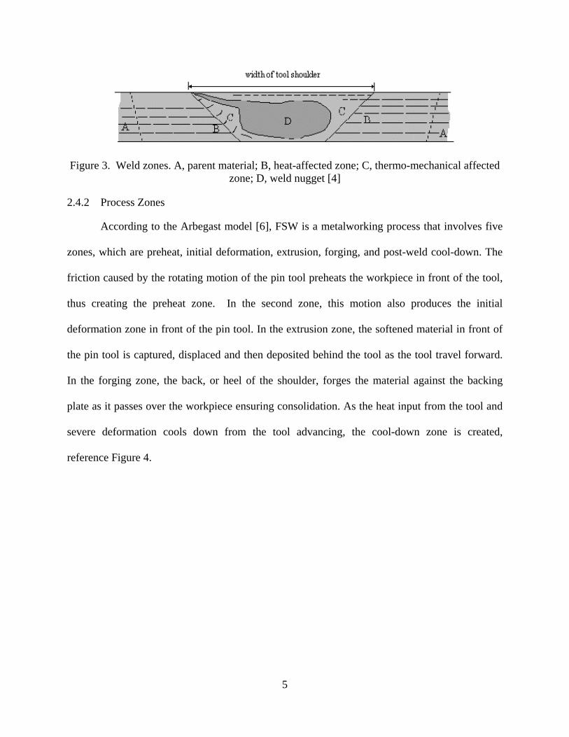
According to the Arbegast model [6], FSW is a metalworking process that involves five
zones, which are preheat, initial deformation, extrusion, forging, and post-weld cool-down. The
friction caused by the rotating motion of the pin tool preheats the workpiece in front of the tool,
thus creating the preheat zone. In the second zone, this motion also produces the initial
deformation zone in front of the pin tool. In the extrusion zone, the softened material in front of
the pin tool is captured, displaced and then deposited behind the tool as the tool travel forward.
In the forging zone, the back, or heel of the shoulder, forges the material against the backing
plate as it passes over the workpiece ensuring consolidation. As the heat input from the tool and
severe deformation cools down from the tool advancing, the cool-down zone is created,
reference Figure 4.
6
Figure 4. Metallurgical processing zones developed during friction stir joining [6].
2.4.3 Metal Flow Zones
Five different metal flow zones have been identified within the transverse section of the
FSW nugget in [4, 7], reference Figure 5. Zone I and II represent the advancing and retreating
side extrusion zones respectively. Zone III is the flow arm where material was dragged across the
nugget. Zone IV is the swirl zone of material processing near and beneath the pin tool tip. Zone I
is filled in by an interleaving pattern of material passing through the other zones, and zone V
(recirculation zone) may form under very hot processing conditions. According to Arbegast [7] if
a wormhole defect forms, it usually occurs at the interface between zone I and zone IV, reference
Figure 6.
Figure 5. Metal flow zones developed during friction stir welding [7]
VV
7
Figure 6. Void formation at the flow zone interfaces [7].
2.5 FSW Imperfections
Even though FSW is a relatively simple process, an inadequate combination of
parameters during welding may produce undesirable results. The types of imperfections observed
depend on the weld configuration. In the butt weld configuration, common imperfections are
voids and wormholes, lack of penetration and joint line remnant defects (also known as kissing
bond, lazy S or entrapped oxide defects) [4, 8]. Some of the defects that can be created in the lap
weld configuration are hooking, sheet thinning, oxide remnant, and voids. In this study, only the
butt weld configuration will be analyzed.
2.5.1 Wormhole Defect and Intermittent Voids
One of the most common defects associated with FSW butt weld configurations is a
wormhole defect [2]. A wormhole, or tunnel defect, that runs along the weld is a cavity below
the weld surface and is attributed primarily to insufficient forming pressure under the tool
shoulder. This prevents the material from fully consolidating [4, 6]. Figure 7 shows a macro
section of a FSW nugget with a wormhole capture with a stereomicroscope. In some cases,
8
especially when welding in displacement control, voids do not form as a continuous wormhole.
Instead, they may appear and disappear periodically, forming intermittent voids.
Figure 7. Macro section of FSW with a wormhole on the advancing side of the weld, red circle
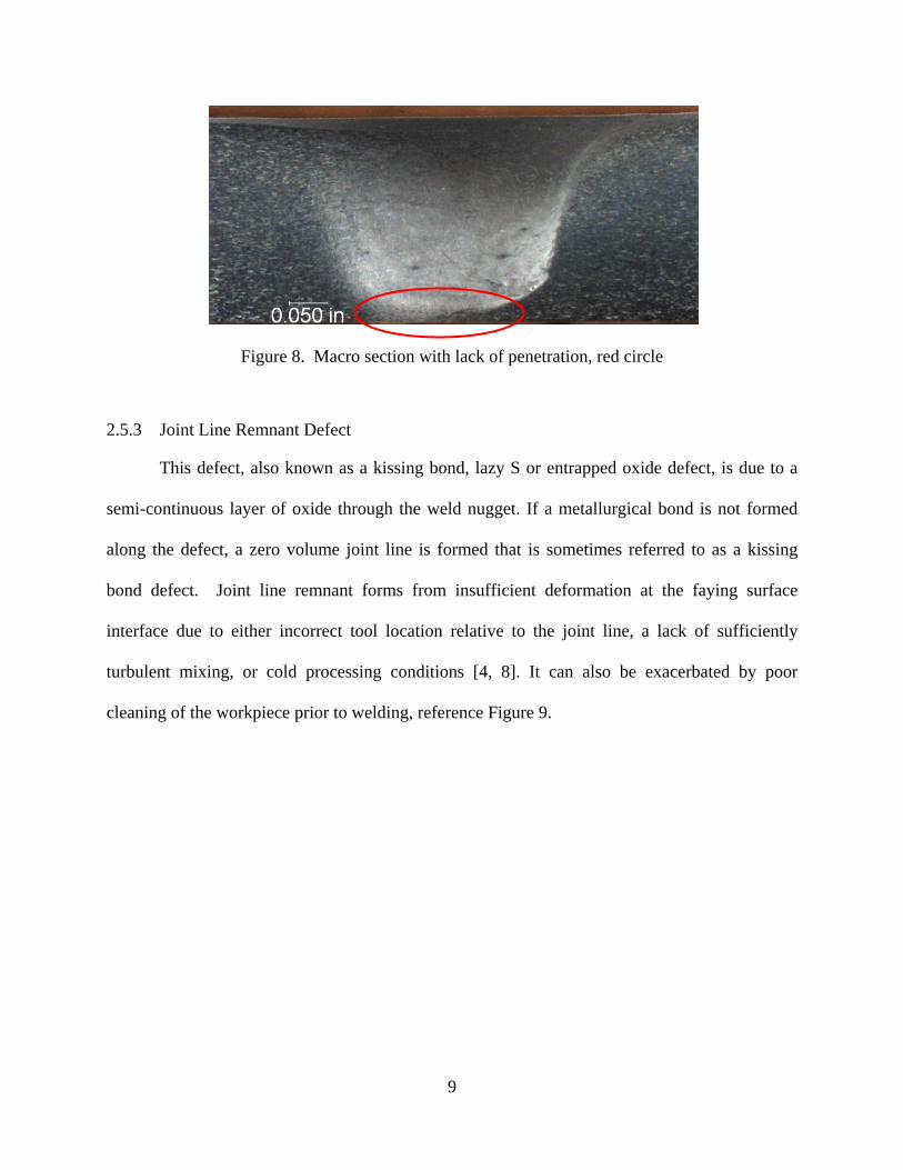
2.5.2 Lack of Penetration Defect
Another common imperfection in FSW butt welds is incomplete root penetration, or lack
of penetration on the root side, leaving a part of the joint line without full consolidation. This can
be caused by insufficient penetration of the pin tool into the workpiece, either by the shortness of
the pin tool for a particular parameter set or a failure to fully engage the pin tool. It can also be
caused by misalignment with the joint line. Similar to the wormhole defect, the lack of
penetration can cause severe weakening of the mechanical properties of the weld because of the
reduction of the cross sectional area within the workpiece. Figure 8 shows a macro section with
a lack of penetration. In this case, it is obvious because the weld nugget is slightly smaller than
the thickness of the parent material, leaving an un-joined remnant.
9
Figure 8. Macro section with lack of penetration, red circle
2.5.3 Joint Line Remnant Defect
This defect, also known as a kissing bond, lazy S or entrapped oxide defect, is due to a
semi-continuous layer of oxide through the weld nugget. If a metallurgical bond is not formed
along the defect, a zero volume joint line is formed that is sometimes referred to as a kissing
bond defect. Joint line remnant forms from insufficient deformation at the faying surface
interface due to either incorrect tool location relative to the joint line, a lack of sufficiently
turbulent mixing, or cold processing conditions [4, 8]. It can also be exacerbated by poor
cleaning of the workpiece prior to welding, reference Figure 9.
10
Figure 9. Joint line remnant in the nugget (identified by arrow)
2.6 Feedback Forces
Feedback forces from the pin tool are measurements of the material resistance forces
induced by the pin tool’s rotation and travel [2]. The feedback forces generally exhibit sinusoidal
oscillations [2, 7, 9]. The feedback force acting on the travel direction against the pin tool is Fx.
The feedback force acting perpendicular to the travel direction is Fy, and is the measure of the
side to side motion. Perpendicular to the plane containing Fx and Fy forces is the Fz force, which
represent the forging force of the tool. With the help of the right hand rule, the positive direction
for these forces can be obtained, reference Figure 10.
11
Figure 10. Fx, Fy, and Fz feedback forces generated by the pin tool [2].
During the welding process, when the welder is equipped with sensors capable of
collecting the feedback forces, this measurement can be collected for analysis. The repeatable
and cyclical nature of the material flow patterns in FSW and their relationship to process forces
provide an opportunity to develop intelligent FSW algorithms which include sensing and
feedback control systems [7].
Arbegast also found that an increase in Fx is related to faster travel speeds and colder
processing conditions [7]. On the other hand, with hotter processing conditions, the softer the
material the lower the Fx is. An increase in Fy is an indication of force imbalance of flow from
the advancing to the retreating side of the weld. These imbalances cause perturbations in the flow
12
pattern, manifesting as fluctuations in the magnitude and direction of processing forces. From
this, it is observed that as the flow becomes less well behaved void formation begins to occur,
creating greater imbalances which in turn increase the magnitude of Fy.
Morihana [9] has analyzed the Fx, Fy and Fz force magnitudes and directions developed
during FSW in frequency space using Fourier Transformation techniques and has demonstrated a
correlation to weld quality. In his study, the presence of very low frequency force events was
correlated to the presence of wormhole defects. Jene et al [10] also gave evidence that frequency
spectra of feedback forces have a high potential for monitoring weld quality. In Figure 11, it can
be seen how the amplitude of the low frequency oscillations increases, relative to spindle
frequency, when a wormhole is forming.
Figure 11. Frequency spectra of Y force with the corresponding metallographic images. The
vertical axis is the amplitude normalized by the maximum amplitude. The spindle peak is located at 4.16 Hz (250 rpm). Amplitude of low frequency oscillations tend to increase while a
wormhole defect starts forming [2]
Spindle Frequency
Low Frequency associated with defect
13
2.7 Non-Destructive Evaluation (NDE)
Presently, a variety of control methods are being applied to ensure the quality of friction
stir welding. In high volume fabrication and/or in sensitive parts, cost of quality control can be a
very important factor in the equation to decide which method will be applied. Two of the most
reliable techniques applied in industry today are Ultrasonic Phased Array (UPA) and X-ray
inspection.
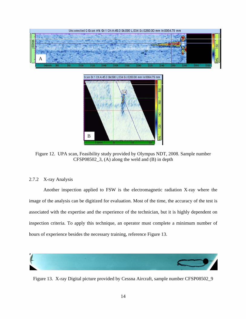
2.7.1 Ultrasonic Phased Array Analysis
One of the non destructive techniques successfully applied to FSW is ultrasonic phased
array (UPA) [12, 13, 14]. This powerful technique is widely applied to FSW because of its
capability to detect the size and location of different kinds of FSW defects. It provides the
coverage and the speed required reliably. Also, UPA maximizes the probability of detection of
flaws by adjusting the inspection angles and eliminates the need for a second scanning axis, as
scanning setups are done electronically. However, the accuracy of the test is associated with the
training, expertise and the experience of the technician. It is also highly dependent on test setup.
To apply this technique, an operator should have considerable experience in weld inspections,
besides the necessary training. An UPA scan performed by Olympus NDT from the crown side
(tool shoulder side) of the weld can be seen in Figure 12. In (A) the wormhole can be seen along
the weld and in (B) the wormhole is shown on a transverse image at depth.
14
Figure 12. UPA scan, Feasibility study provided by Olympus NDT, 2008. Sample number CFSP08502_3, (A) along the weld and (B) in depth
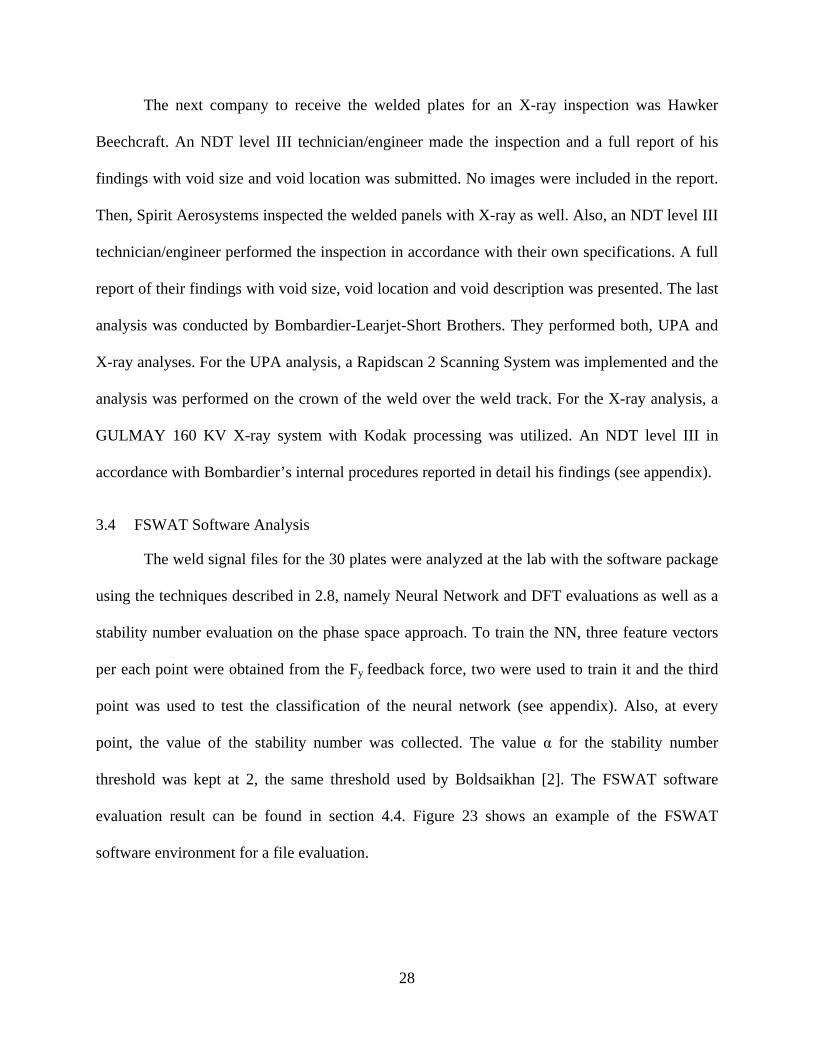
2.7.2 X-ray Analysis
Another inspection applied to FSW is the electromagnetic radiation X-ray where the
image of the analysis can be digitized for evaluation. Most of the time, the accuracy of the test is
associated with the expertise and the experience of the technician, but it is highly dependent on
inspection criteria. To apply this technique, an operator must complete a minimum number of
hours of experience besides the necessary training, reference Figure 13.
Figure 13. X-ray Digital picture provided by Cessna Aircraft, sample number CFSP08502_9
B
A
15
2.7.3 FSWAT Software, Real Time NDE
The Friction Stir Welding Analysis Tool software was built using Microsoft Visual
C++.NET and implements the algorithms discussed in Section 2.8. The FSWAT has the
capability to read all feedback forces recorded as data files during the welding process. It was
designed to analyze any specified section of the weld in real time (with a slight computation
delay) in a non-destructive manner. The tools provided by the software for conducting the
analysis are the frequency-spectrum analysis, the phased space analysis and the autocorrelation
and cross-correlation functions. The frequency-spectrum analysis tool calculates the Discrete
Fourier Transformation (DFT), graphically displays the analysis, and extracts feature vectors
from the DFT. Feature vectors are n-dimensional vector of numerical features that represent
some object. The phase-space analysis tool plots the phase plane of time series data versus its
time derivative. In addition, the phase-space analysis tool calculates a stability number and the
time gap of the feedback forces described by Boldsaikhan [2].
2.8 The Algorithms Applied In FSWAT
As mentioned above, the FSWAT implements the algorithms discussed by Boldsaikhan
[2,15,16]. These include the use of a Neural Network (NN) - Discrete Fourier Transformation
(DFT) technique and the Phase Space based approach for real time evaluation of friction stir
welding and is discussed in the next section. .
2.8.1 NN and DFT for Real Time Evaluation of FSW
This algorithm consist of two procedures, the first is to extract a feature vector from the
frequency spectra of the feedback forces and the second is to employ a multilayer NN trained
with the error-back propagation method. As stated by Boldsaikhan, the advantage of
16
implementing a NN is the possibility of defining a problem empirically by using sufficient
examples, rather than describing it analytically [2].
Boldsaikhan et al. implemented the use of NN, a well known classification method, to
show that oscillation of feedback forces can be used to evaluate weld quality [15]. In his
investigation, the use of Fx feedback forces extracted from the weld data was demonstrated to be
a good feedback signal to evaluate tensile strength at three levels (good, satisfactory or bad) with
90% correctly classified using a NN. Also in the same investigation, using a neural network the
Fy feedback force was shown to correctly classify 100% of the welds containing wormholes.
Figure 14 shows a multilayer neural network.
Figure 14. Multilayer neural network for detecting wormhole defects
2.8.2 Phase Space and Time Gap Analysis
The phase space algorithm used on the FSWAT has two procedures. The first procedure
is to determine the stability of the X and Y forces using the Poincaré map method. The second
procedure is to measure the time gap. The decision logic of the phase-space-based analysis
algorithm is shown in Figure 15.
17
Figure 15. Decision logic for the phase space approach
In Figure 15, the variables α and β stand for empirical parameters for the stability number
and the time gap. Theses parameters were set at α = β = 2 by Boldsaikhan and showed a good
correlation in his research [2, 16].
2.8.2.1 The Phase Space
The phase space is the plot of the feedback force against its own time derivative and
shows the dynamics of a variable changing through time. In FSW, a phase space plot can be
defined by:
• Fx force x
• Time-derivative of Fx force: dx/dt
• Fy force y
• Time-derivative of Fy force: dy/dt
The curves formed by plotting a variable against its derivative through time are known as
trajectories or orbits. As a simple example, plotting the function f(t)=sin(t) against its derivative
df/dt=cos(t) will produce a circle. When a system is stable (e.g. periodic), the trajectories tend to
18
overlap each other tightly on circular paths. If the system is unstable, however, the paths will
separate.
As presented before, the Fy force feedback is the most closely correlated to metallurgical
quality [7]. This is the main reason why phase space analysis was applied to quantify the
instability of the Y force feedback in the research of Boldsaikhan et al. [16]
2.8.2.2 The Poincaré Map
To quantify the instability of the system in the phase space, Boldsaikhan et al [16]
applied the Poincaré Map method, which is used to locate a hyperplane orthogonal to the
direction of the trajectory. With periodic and stable trajectories a repeated intersection on the
hyperplane at the same point can be obtained. As the orbits start to lose periodicity (or as the
orbits do not return over the same trajectory), a cluster of points will appear on the hyperplane.
The Poincaré Map is also called the “first return” map, reference Figure 16.
Figure 16. First return map or Poincaré map.
A method of characterizing the distribution pattern of the points is to calculate the
standard deviation of the cluster. The standard deviation can be calculated as:
σ A
Eq. 1 [16].
19
Where σ1 is the standard deviation of the cluster from the bottom to the top piercing or
intersection; A is the amplitude of the spindle frequency oscillation.
2.8.2.3 The Phase Space Approach
The quantity that defines the stability of the feedback forces is the stability number [2].
Figure 17 shows a schematic process to calculate the stability number based on a selected, or
Windowed, range of the raw force feedback data.
Figure 17. Schematic process to calculate the Stability Number [2]
The stability number of the feedback forces was defined by Boldsaikhan as shown in
Equation 2 and can be calculated from [2]:
Eq. 2
Where:
σx sample standard deviation of local maximum points of X forces
Ax amplitude of the spindle frequency oscillation of X forces
σy sample standard deviation of local maximum points of Y forces
Ay amplitude of the spindle frequency oscillation of Y forces
20
2.8.2.4 The Time Gap
The second procedure used on the phase space approach is to measure the time gap. The
time gap was defined by Boldsaikhan as the divergence between the deposition time plus the
equilibrium time and the time that the spindle spends in an entire rotation (the sum of the
origination time and the deposition time) [2]. During the period of time called the “origination
time”, Fy decreases with the flow of material from the leading side to the trailing side (see Figure
18). Conversely, in the period of time called the “deposition time”, material flows from the
trailing side to the leading side causing Fy to increase, reference Figure 18. In an ideal situation
the origination time and the deposition time will be equal, and both will be equal to half of the
spindle period. Further, the equilibrium time of a weld will be half of the spindle frequency.
Then, in order to have a good weld the difference between the equilibrium time and the
deposition time should be zero or near zero.
Figure 18. Shear forces relating to Fy feedback force [2]
21
3 OBJECTIVE AND METHODS
3.1 Objective
The purpose of this study is to determine if the defects found using the non-destructive
evaluation techniques, ultrasonic phased array and X-ray inspection, can be identified by the
FSWAT software. The ultimate goal of this research is to support the development of real time
quality control to minimize the cost of inspection through statistical process control methods.
3.2 Methodology
In this project, feedback force signals provided by the MTS® ISTIR™ PDS welding
machine located at the Advanced Joining and Processing Lab (AJP) at the National Institute for
Aviation Research (NIAR), Wichita State University, were analyzed with the FSWAT software
and soon after compared with the results of NDE as well as destructive tests. Unlike the study
performed by Boldsaikhan [2,15,16], where the welds were created using a cylindrical threaded
pin tool, the software analysis in this project deals with tool differences, a different aluminum
alloy, and the addition of a comparison with existing NDE techniques. A stability number
evaluation of the phase space approach and a DFT- neural network training and classification
was performed on the feedback force data.
3.2.1 Experimental Procedure
The experiment consisted of friction stir weld in a butt weld configuration using five
different tools to create ten different welds, each with a unique combination of processing
parameters for welding 0.25 inch thick aluminum alloy AA2024-T351. Each weld was repeated
three times for a total of 30 welded plates in order to study the repeatability of the defects and
analysis. The tools and the welding parameters were selected from the path independent work of
22
Widener et al. performed in the NIAR AJ&P Lab [1]. The tools vary widely in both pin and
shoulder features. The tools had the following distinguishing features:
1. Classic TWI 5651 probe and shoulder
2. TWI Tri-flute™ probe with a scrolled shoulder
3. A scrolled shoulder and a probe with threads and straight flats
4. A small diameter Wiper™ shoulder and a probe with threads and twisted flats
5. A large diameter Wiper™ shoulder and a probe with threads and twisted flats
These tools are shown in the Figure 19 below. Also, a graphic with the set of welding parameters
utilized for each of the five tools respectively can be seen in Figure 20.
Figure 19. Tool design [1]
23
Figure 20. Set of welding parameters for the five different tools respectively.
For this work, the capture rate of feedback forces of the MTS ISTIR was set as 10 times
the frequency of the spindle speed for every weld as a standard. Boldsaikhan in [2]
recommended that the capture rate should not be less than 8 times the spindle frequency for a
good analysis. This was done to account for every group of welds having different welding
parameters. For example, data from a 600 RPM (10 Hz) weld would be captured at 100 Hz while
data from a 300 RPM (5 Hz) weld would be captured at 51.2 Hz (which is the closest available
capture rate on the MTS ISTIR to 50 Hz).
Every welded plate was analyzed with the FSWAT software in the lab. The UPA analysis
as well as the X-ray analysis was performed by technicians/engineers in a round robin
investigation with the participation of Olympus NDT, Cessna Aircraft Company, Hawker
Beechcraft, Spirit Aerosystems, and Bombardier-Learjet-Short Brothers. After the round robin
24
investigation was completed the result were verified by metallographic inspection and correlated
with mechanical test results performed in the AJP lab. Finally, probability of detection curves
were constructed as a statistical evaluation for each of the non-destructive inspection techniques.
3.2.2 Weld Preparation
Plates of aluminum alloy AA2024-T351 of 12 in. by 4 in. with a thickness of 0.25 in.
were welded together in a butt weld configuration. The welding parameters utilized for each pin
tool were different and derived from the results of previous work [1]. Table 1 shows the original
NIAR AJ&P Lab work order number from where the parameters were obtained. It also included
the pin tool design and the new NIAR AJ&P Lab work order number utilized to create the
“good” and “bad” welds for the project.
3.3 NDE Round Robin Investigation
Once all the plates were welded, they were sent to each of the participants of the NDE
round robin investigation as a complete set of 30 plates for analysis. The only instruction
regarding the analysis that the companies received was to inspect the welded region for defects
per their own internal specifications, and to provide a report detailing their findings.
Olympus NDT conducted an UPA demonstration on only two plates as a feasibility study
in the initial stages of the project. Since they only inspected two of the 30 plates, their findings
were not included in the overall analysis; however, their results were used as a qualitative
comparison with the other UPA and X-ray results published by Gimenez, Widener, Brown and
Burford [20]. The plates were immersed in water and scanned from the crown and root side of
the weld over the weld track of the plate on a single scan using a mini-wheel encoder. Figure 21
shows the Omniscan MX from Olympus NDT as well as the test set up.
25
The first company that analyzed the welded plates for the round robin investigation was
Cessna Aircraft Company using both UPA and X-ray analysis. The UPA analysis was also
performed in immersion, just like Olympus NDT. The plates were scanned from the crown side
of the weld on the advancing and retreating sides of the weld track, as shown in Figure 22. The
X-ray analysis at Cessna Aircraft was performed with a Digitized Film Radiography Kodak M
film, 60 seconds flat exposure. A digital file with the actual images from the UPA and the X-ray
inspection were received, and measurements of the void locations were extracted from those
images.
26
Table 1. List of work order (expected good weld are highlighted)
original work order equivalent work order tool1 FSW07026_2 FSW08502_1 wiper2 FSW07026_2 FSW08502_33 wiper3 FSW07026_2 FSW08502_34 wiper
The sources of noise in the feedback force signals of FSW could be the result of clamping
forces, pin tool wear or damage, anvil damage, or vibration on the welding machine. The best
alternative to deal with undesirable noise is to work on the noise generation. Noise that comes
from the vibration of the welding machine is a more challenging issue and may require more
technology to isolate the vibration. In any alternative, it is always desirable to avoid any noise
generation in the feedback force signal than to filter it.
3.6.2 Repetition of NDE techniques
During the round robin investigation, it was possible to perform four different X-ray
analyses in different locations and two ultrasonic phased array analyses in different locations as
well. For the final project analysis, however, only three X-ray analysis results and one UPA
result were utilized, due to incompatibility of reporting methods as described in Section 4.4.
34
4 RESULTS
4.1 Inspection Reports
As mentioned in Section 3.3 the participants of the round robin investigation presented a
report of the techniques applied in their facility. Copies of those reports are included in the
appendix. An example of an indication reported by Olympus NDT using UPA analysis is shown
in Figure 26. In this case, the flaw starts at 8.7 in. (222 mm) from the beginning of the plate and
continues to the end of the plate, indicated in the red circle.
Figure 26. Indication of void (in red), UPA inspection. Work order number CFSP08502_03 welded with Wiper™-large pin tool. Olympus NDT feasibility study.
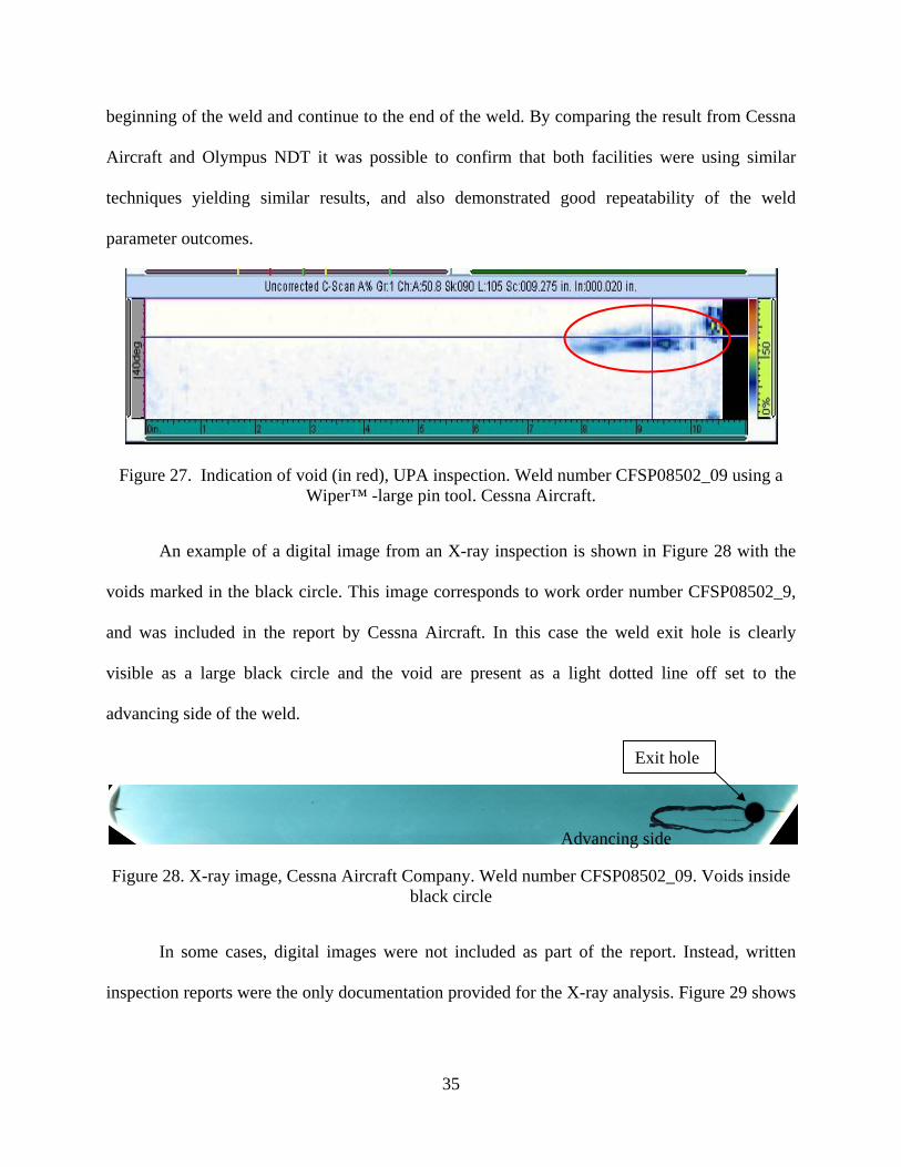
Next, Figure 27 shows the UPA analysis carried out by Cessna Aircraft Company. This
analysis was completed on work order number CFSP08502_9, which has the same welding
parameters and pin tool as CFSP08502_03 analyzed by Olympus NDT (Figure 26Figure 26). In
the report presented by Cessna Aircraft, the flaws are located at 7.7 in. (195 mm) from the
35
beginning of the weld and continue to the end of the weld. By comparing the result from Cessna
Aircraft and Olympus NDT it was possible to confirm that both facilities were using similar
techniques yielding similar results, and also demonstrated good repeatability of the weld
parameter outcomes.
Figure 27. Indication of void (in red), UPA inspection. Weld number CFSP08502_09 using a Wiper™ -large pin tool. Cessna Aircraft.
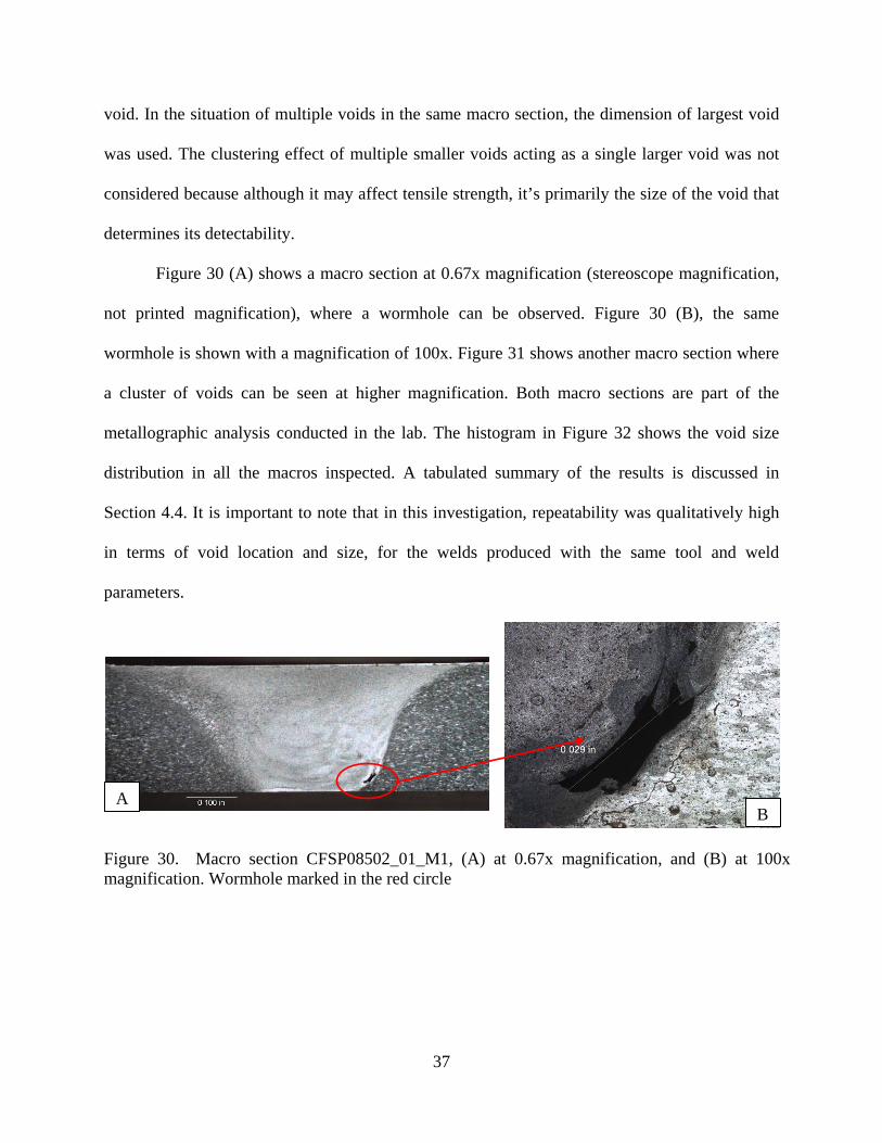
An example of a digital image from an X-ray inspection is shown in Figure 28 with the
voids marked in the black circle. This image corresponds to work order number CFSP08502_9,
and was included in the report by Cessna Aircraft. In this case the weld exit hole is clearly
visible as a large black circle and the void are present as a light dotted line off set to the
advancing side of the weld.
Figure 28. X-ray image, Cessna Aircraft Company. Weld number CFSP08502_09. Voids inside black circle
In some cases, digital images were not included as part of the report. Instead, written
inspection reports were the only documentation provided for the X-ray analysis. Figure 29 shows
Exit hole
Advancing side
36
part of the detailed report of the X-ray analysis carried out and presented by Hawker Beechcraft,
Spirit Aerosystems, and Short Brothers-Bombardier respectively (see appendix).
4.2 Metallographic Result
Every macro section was inspected at the lab looking for the presence of voids or
wormholes. The longest dimension in a void in any direction was considered as the size of the
Figure 29. X-ray inspection Reports presented by Hawker Beechcraft, Spirit Aerosystems, and Bombardier-Learjet-Short Brothers respectively
37
void. In the situation of multiple voids in the same macro section, the dimension of largest void
was used. The clustering effect of multiple smaller voids acting as a single larger void was not
considered because although it may affect tensile strength, it’s primarily the size of the void that
determines its detectability.
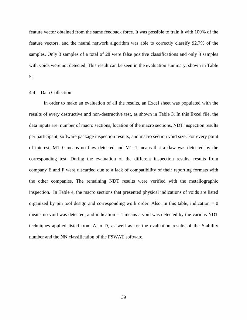
Figure 30 (A) shows a macro section at 0.67x magnification (stereoscope magnification,
not printed magnification), where a wormhole can be observed. Figure 30 (B), the same
wormhole is shown with a magnification of 100x. Figure 31 shows another macro section where
a cluster of voids can be seen at higher magnification. Both macro sections are part of the
metallographic analysis conducted in the lab. The histogram in Figure 32 shows the void size
distribution in all the macros inspected. A tabulated summary of the results is discussed in
Section 4.4. It is important to note that in this investigation, repeatability was qualitatively high
in terms of void location and size, for the welds produced with the same tool and weld
parameters.
Figure 30. Macro section CFSP08502_01_M1, (A) at 0.67x magnification, and (B) at 100xmagnification. Wormhole marked in the red circle
A B
38
Figure 32. Histogram of void size distribution
4.3 Neural Network Classification Result
As mentioned in Section 3.4 the Neural Network algorithm of the FSWAT software was
trained with two feature vectors obtained from the Fy feedback force and was tested with one
Histogram
void size
frequ
ency
0 0.02 0.04 0.06 0.080
5
10
15
20
25
30
Figure 31. Macro section CFSP08502_06_M2, (A) at 0.67x magnification, and (B) at 100xmagnification. Wormholes market in the red circle
A B
39
feature vector obtained from the same feedback force. It was possible to train it with 100% of the
feature vectors, and the neural network algorithm was able to correctly classify 92.7% of the
samples. Only 3 samples of a total of 28 were false positive classifications and only 3 samples
with voids were not detected. This result can be seen in the evaluation summary, shown in Table
5.
4.4 Data Collection
In order to make an evaluation of all the results, an Excel sheet was populated with the
results of every destructive and non-destructive test, as shown in Table 3. In this Excel file, the
data inputs are: number of macro sections, location of the macro sections, NDT inspection results
per participant, software package inspection results, and macro section void size. For every point
of interest, M1=0 means no flaw detected and M1=1 means that a flaw was detected by the
corresponding test. During the evaluation of the different inspection results, results from
company E and F were discarded due to a lack of compatibility of their reporting formats with
the other companies. The remaining NDT results were verified with the metallographic
inspection. In Table 4, the macro sections that presented physical indications of voids are listed
organized by pin tool design and corresponding work order. Also, in this table, indication = 0
means no void was detected, and indication = 1 means a void was detected by the various NDT
techniques applied listed from A to D, as well as for the evaluation results of the Stability
number and the NN classification of the FSWAT software.
As shown in Table 5, the detection rate of the stability number using the phase space
approach for this investigation is low. This may be the result of an unadjusted threshold value, α,
since α may vary for different pin tool designs; however, α was not investigated, instead the
threshold value of α was set at 2 following previous work [2]. An investigation of the variation
of the stability number threshold per pin tool design is expected to be the subject of a future
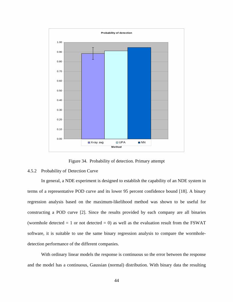
investigation. For this reason Figure 34 shows only the POD of the X-ray (average), the UPA
and the NN- DFT classification, but the stability number result is not shown. Note: the X-ray
analysis is the only test repeated three times by different participants with an average of 88% of
detection and a standard deviation of 5.8%.
44
Figure 34. Probability of detection. Primary attempt
4.5.2 Probability of Detection Curve
In general, a NDE experiment is designed to establish the capability of an NDE system in
terms of a representative POD curve and its lower 95 percent confidence bound [18]. A binary
regression analysis based on the maximum-likelihood method was shown to be useful for
constructing a POD curve [2]. Since the results provided by each company are all binaries
(wormhole detected = 1 or not detected = 0) as well as the evaluation result from the FSWAT
software, it is suitable to use the same binary regression analysis to compare the wormhole-
detection performance of the different companies.
With ordinary linear models the response is continuous so the error between the response
and the model has a continuous, Gaussian (normal) distribution. With binary data the resulting
Probability of detection
0.00
0.10
0.20
0.30
0.40
0.50
0.60
0.70
0.80
0.90
1.00
1
Method
X-ray avg UPA NN
45
error between observation and model prediction is decidedly non-normal (it’s binomial) and so
treating it as Gaussian would produce inaccurate and unreliable parameter estimates, even when
the model is restricted to realistic values (0 < y <1). Generalized Linear Models (GLM)
overcome this difficulty by “linking” the binary response to the explanatory variables through
the probability of either outcome 0 or 1. The transformed probability can then be modeled as an
ordinary polynomial function, linear in the explanatory variables, and so it is a generalized linear
model [23].
The software package R mh1823POD [24] algorithms implement four links to map -∞ <
x < ∞ into 0 < y <1. The four links are the logit, logistic or log-odds function, the probit or
inverse normal function, the complementary log-log function, often called Weibull by engineers,
and the loglog function. For this work the Logit link was implemented (scatter in the plotted
binary values is for graphic purposes only):
Logit log Eq. 4
In Eq. 4, f (a) is any appropriate algebraic function which is linear in the parameters
where a is the void size, μ is the mean and is the standard deviation of the sample. Often, but
not always, this is a polynomial. In Eq. 5, ( ) is the logistic sigmoid function. The probability
of detection, pi = POD (ai), is define as a function linked to the ith void size, ai. The mh1823
POD software uses the logit link for POD (a, ...).
logit link , … Φ a Eq. 5
46
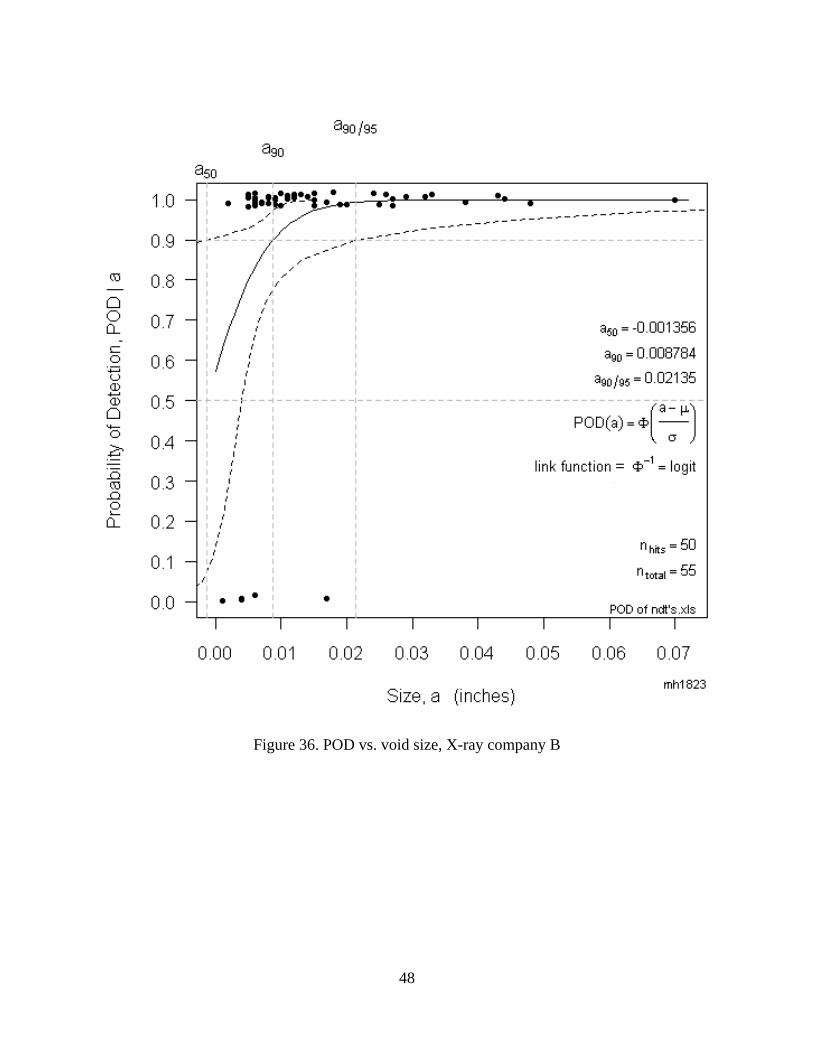
4.5.2.1 X-ray POD Results
POD vs. void size for each of the three X-ray inspections is plotted in Figure 35 - Figure
37; where the minimum void size detected by each company is shown. The mean POD
calculated from all company results is the solid line and its lower bound is the dashed line. For
company A (Figure 35), it is believed that the increased standard deviation with the increase in
defect size was just a type three mistake (i.e. a mistake in reporting) in this analysis, since the
larger the void is the easier it is to detect.
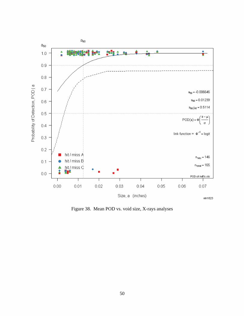
Next, a mean POD vs. void size with its lower 95% bound applied to the three X-ray
analysis results is plotted in Figure 38. The minimum void size that was detected with 90% POD
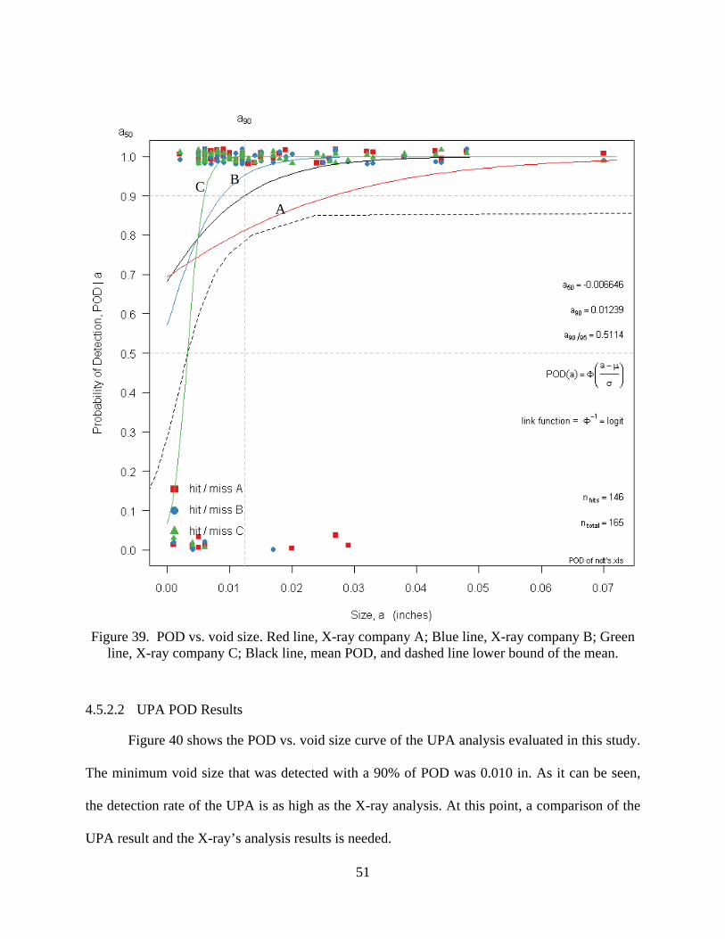
was 0.012 in. Then, in Figure 39, the plot of the three X-ray inspections all together, as well as
the mean POD, is shown. Graphically, the POD curve shows that there is no significant
difference within the X-ray results at any point of the curve since all three company results lie
within the 95% confidence interval of the mean for a void size larger than 0.003 in. These results
correspond to the current practices of X-ray analysis being applied in industry.
47
Figure 35. POD vs. void size, X-ray company A
48
Figure 36. POD vs. void size, X-ray company B
49
Figure 37. POD vs. void size, X-ray company C
50
Figure 38. Mean POD vs. void size, X-rays analyses
51
Figure 39. POD vs. void size. Red line, X-ray company A; Blue line, X-ray company B; Green
line, X-ray company C; Black line, mean POD, and dashed line lower bound of the mean.
4.5.2.2 UPA POD Results
Figure 40 shows the POD vs. void size curve of the UPA analysis evaluated in this study.
The minimum void size that was detected with a 90% of POD was 0.010 in. As it can be seen,
the detection rate of the UPA is as high as the X-ray analysis. At this point, a comparison of the
UPA result and the X-ray’s analysis results is needed.
C A
B
52
Figure 40. POD vs. void size, UPA analysis
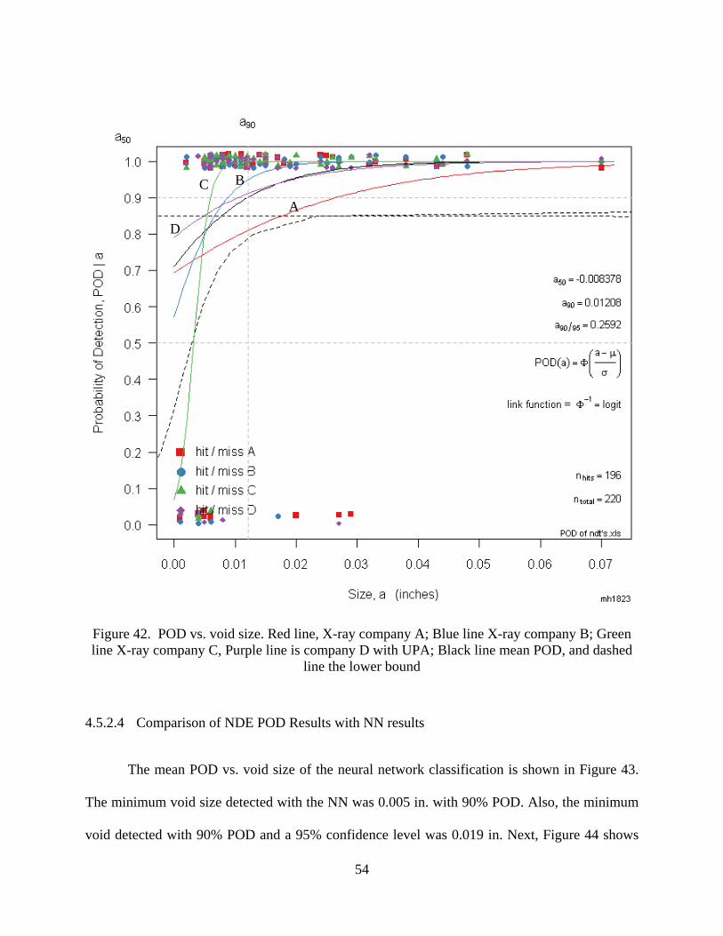
4.5.2.3 Combined X-ray & UPA POD Results
In Figure 41 the mean POD vs. void size of the one UPA result and the three X-ray
analysis results are compared. The minimum void size that was detected with 90% of POD was
0.012 in. The same minimum void size detected by the three X-ray analyses is shown in Figure
38. Figure 42 shows the POD curve of all three X-ray analysis results (red, blue and green line)
as well as POD curve of the UPA analysis result. Graphically, the POD curve shows that there is
53
no significant difference within the X-ray results and the UPA at any point of the curve since all
three company results lie within the 95% confidence interval of the mean for a void size larger
than 0.003 in.
Figure 41. Mean POD vs. void size; X-ray's and UPA analysis results
54
Figure 42. POD vs. void size. Red line, X-ray company A; Blue line X-ray company B; Green line X-ray company C, Purple line is company D with UPA; Black line mean POD, and dashed
line the lower bound
4.5.2.4 Comparison of NDE POD Results with NN results
The mean POD vs. void size of the neural network classification is shown in Figure 43.
The minimum void size detected with the NN was 0.005 in. with 90% POD. Also, the minimum
void detected with 90% POD and a 95% confidence level was 0.019 in. Next, Figure 44 shows
A
B C
D
55
the mean POD of the NN, the UPA and the X-ray analysis results. The minimum void size that
was detected with a 90% POD was a 0.011 in with the combined results.
Figure 43. POD vs. void size, neural network classification
56
Figure 44. Mean POD vs. void size. NN, UPA (company D) and X-ray (A, B, and C) analysis results
In order to make a comparison between all the NDE techniques applied in this work, all
the NDE POD curves were plotted together, Figure 45. Graphically, the POD curves show that
there is no significant difference observed for this project within any of the techniques applied at
57
any point of the curve since all the results lie within the 95% confidence interval of the mean for
a void size larger than 0.003 in.
Figure 45. POD vs. void size. Red line, X-ray company A; Blue line X-ray company B; Green
line X-ray company C, Purple line UPA company D; Orange line NN; Black line mean POD and dashed line lower bound
A
B
C
D NN
58
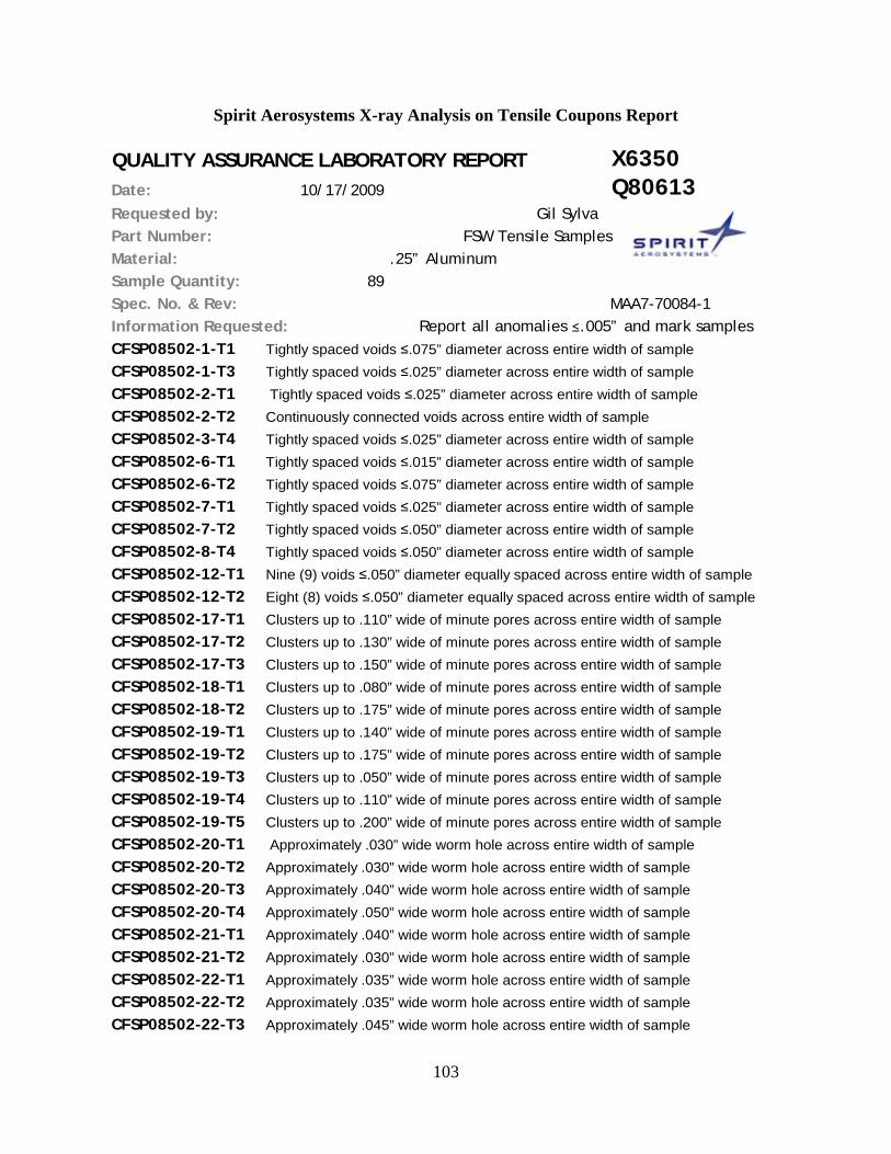
4.5.3 Tensile Test
An in house report was prepared for the tensile test results. A portion of the data is
shown in Table 6, but the complete table is in the appendix. Besides the tensile result report,
Spirit Aerosystems submitted the report of the X-ray analysis performed on the coupons. A
portion of the report is shown in Table 7, but the complete table is given in the appendix.
CFSP08502-1-T1 Tightly spaced voids ≤.075” diameter across entire width of sampleCFSP08502-1-T3 Tightly spaced voids ≤.025” diameter across entire width of sampleCFSP08502-2-T1 Tightly spaced voids ≤.025” diameter across entire width of sampleCFSP08502-2-T2 Continuously connected voids across entire width of sampleCFSP08502-3-T4 Tightly spaced voids ≤.025” diameter across entire width of sampleCFSP08502-6-T1 Tightly spaced voids ≤.015” diameter across entire width of sampleCFSP08502-6-T2 Tightly spaced voids ≤.075” diameter across entire width of sampleCFSP08502-7-T1 Tightly spaced voids ≤.025” diameter across entire width of sampleCFSP08502-7-T2 Tightly spaced voids ≤.050” diameter across entire width of sampleCFSP08502-8-T4 Tightly spaced voids ≤.050” diameter across entire width of sampleCFSP08502-12-T1 Nine (9) voids ≤.050” diameter equally spaced across entire width of sampleCFSP08502-12-T2 Eight (8) voids ≤.050” diameter equally spaced across entire width of sampleCFSP08502-17-T1 Clusters up to .110” wide of minute pores across entire width of sampleCFSP08502-17-T2 Clusters up to .130” wide of minute pores across entire width of sampleCFSP08502-17-T3 Clusters up to .150” wide of minute pores across entire width of sampleCFSP08502-18-T1 Clusters up to .080” wide of minute pores across entire width of sampleCFSP08502-18-T2 Clusters up to .175” wide of minute pores across entire width of sampleCFSP08502-19-T1 Clusters up to .140” wide of minute pores across entire width of sampleCFSP08502-19-T2 Clusters up to .175” wide of minute pores across entire width of sampleCFSP08502-19-T3 Clusters up to .050” wide of minute pores across entire width of sampleCFSP08502-19-T4 Clusters up to .110” wide of minute pores across entire width of sampleCFSP08502-19-T5 Clusters up to .200” wide of minute pores across entire width of sampleCFSP08502-20-T1 Approximately .030” wide worm hole across entire width of sampleCFSP08502-20-T2 Approximately .030” wide worm hole across entire width of sampleCFSP08502-20-T3 Approximately .040” wide worm hole across entire width of sampleCFSP08502-20-T4 Approximately .050” wide worm hole across entire width of sample
MAA7-70084-1Information Requested: Report all anomalies ≤.005” and mark samples
Requested by:Part Number:Material:
Spec. No. & Rev:
The criterion for tensile test classification is as follow: T=0 coupons with high tensile
strength with or without wormhole, T=1 coupon with low tensile strength, macro section and X-
ray showing wormhole. Coupons with low tensile strength without wormhole were neglected.
Low tensile strength in FSW is not necessarily due to the presence of a void or a wormhole but
also can be the result of welding parameter selection. A tensile strength value was considered
low if it was less than 60.9 ksi, which was a minimum design allowable for tensile strength
60
calculated from previous work [1]. In the current study, welding parameter optimization is not
under consideration. Table 8 shows the summary of the tensile classification based on the
mentioned criterion.
Table 8. Tensile classification summary
Tensile classification summary number of tensile 82 in use for the analysis 71 neglected (low tensile strength, no void) 11 tensile with void and high tensile strength (T=0) 25 tensile not affected by void 7 tensile affected by the voids (T=1) 46
The classification of the tensile strength result helped to construct a POD curve of tensile
strength being affected by a wormhole or void as it increases in size. The same binary regression
analysis based on the maximum-likelihood method was applied to the tensile binary result
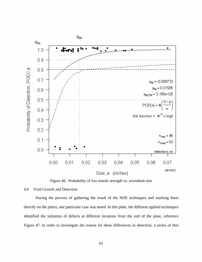
obtained. Figure 46 shows the probability of detection of low tensile strength due to wormhole
size. As shown, a wormhole larger than 0.015 inches has 90% POD of causing low tensile
strength. As discussed before, the presence of small voids is not always detrimental to tensile
strength. It can also be seen in Figure 46 where in some cases voids up to 0.019 in. did not affect
the tensile strength for certain tool and weld parameter combinations.
61
Figure 46. Probability of low tensile strength vs. wormhole size
4.6 Void Growth and Detection
During the process of gathering the result of the NDE techniques and marking them
directly on the plates, one particular case was noted. In this plate, the different applied techniques
identified the initiation of defects at different locations from the end of the plate, reference
Figure 47. In order to investigate the reason for these differences in detection, a series of thin
62
slice macro sections were prepared to evaluate the presence of voids in this region, reference
Figure 48.
Figure 47. Plate CFSP08502-1 marked with variable inspection results
Figure 48. Section of the CFSP08502-1 plate with the locations of thin macro sections
T3
63
With this destructive technique it was possible to observe how a void grows with the tool
travel direction. The series of sections cuts shows the detection of the void can depend on
inspection criteria, experience, technique, equipment resolution, internal standards, etc.
Therefore, the differences in detection for each company for this particular plate can be
understood by looking at the following diagram in Figure 49. This figure demonstrates how
variable void size inspection criteria could result in varying void detection locations as a defect
develops during welding (Note: UPA is sensitive to grain flow and can provide a false positive).
Figure 49. Schematic of evolution of void growth with FSW tool travel distance from the end of the plate
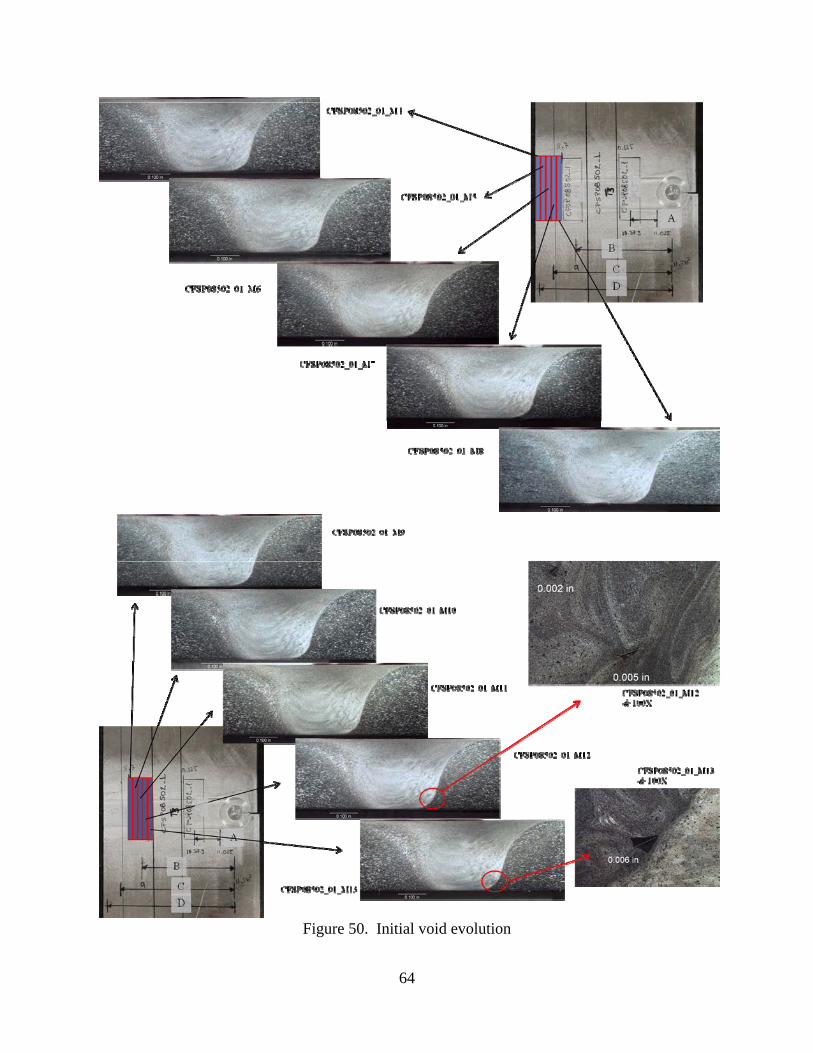
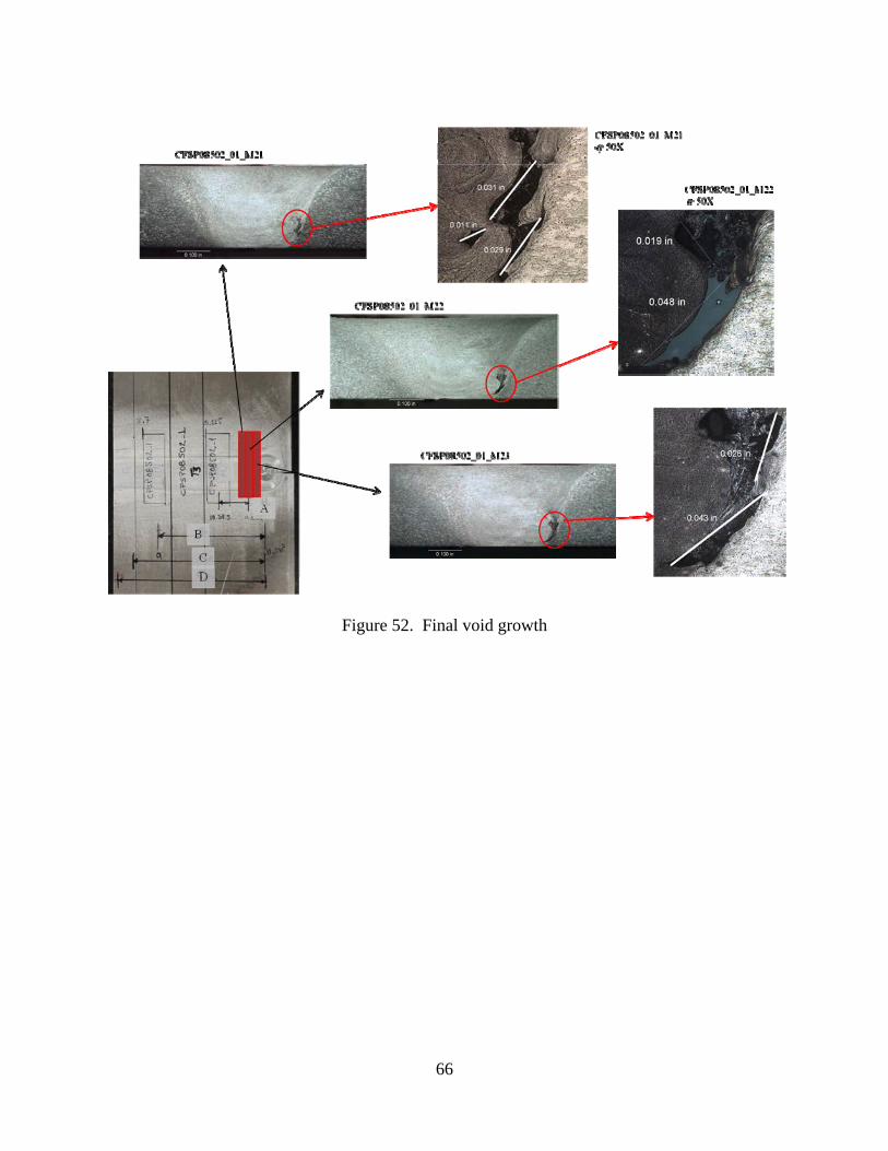
The actual evolution of the void is shown in Figure 50 - Figure 52. The first 8 thin macro
sections did not show any void formation even at a magnification of 200X. This indicates that in
this case, both C and D prematurely indicated the presence of a void. The actual presence of
voids began in the ninth thin macro section and corresponds to the indication made by B. For A,
detection was not indicated until much later in macro section thirteen where a large cluster of
voids was present.
64
Figure 50. Initial void evolution
65
Figure 51. Void growth
66
Figure 52. Final void growth
67
5 CONCLUSION
For this particular study, both non-destructive evaluation techniques applied on friction
stir welding, ultrasonic phased array and X-ray, are effective for void detection in FSW. Both
NDE techniques had basically the same probability of detection of voids with no significant
difference between them; however, the scatter in the result may be larger than desirable. For
instance, scatter was clearly visible when examining the result of the three X-ray analyses.
The minimum void size detected with X-ray with a 90% POD by company A was 0.026
in., but by company C it was 0.006 in. This represents a reduction of 77% in detectable void size.
It is important to note, however, that each company participating in the round robin investigation
followed their own standards for the inspections. The samples were presented to them in a blind
test. Since this was not a competition between companies, this difference most likely represents
simply a difference in inspection criteria or some small space for improvement in the application
of the technique for FSW based on experience with FSW NDE. Based on these results, though,
there is a need for a standard procedure for non-destructive evaluation of FSW and its particular
type of flaws.
The probability of detection of low tensile strength, on the other hand, shows the
probability of getting a low tensile strength because of the presence of void with or without
optimization of welding parameters. In this study, a void size of 0.015 in. had 90% POD
resulting in a low tensile strength. In the X-ray analyses, the mean POD of voids was able to
detect a void size of 0.012 in. with 90% POD. This shows that, in this study, a void that is
capable of causing a reduction in strength can be detected with better than 90% POD. This was
also true of the UPA analysis which was able to detect 0.010 in. void with 90% POD.
68
Consequently, for this application both X-ray and UPA analysis were shown to be effective NDE
techniques for FSW. Nevertheless, there is a need for common FSW inspection criteria and
evaluation methods, which could be provided through an industry specification.
In addition to these current NDE techniques, this study also evaluated both algorithms of
the FSWAT software, Neural Network - Discrete Fourier Transformation, and Phase Space
approach developed at SDSMT by Boldsaikhan. The trained Neural Network classification
shows a very promising result with a very high probability of detection of voids. Also, it is
shown, within the results, that there is no significant difference between the current NDE
techniques and the FSWAT software result. However, a larger sample size could potentially
reduce the scatter in the result.
One of the benefits of the application of the FSWAT software could be the reduction of
100% inspection of the welded pieces for quality control. Since the FSWAT software can be
applied almost in real time along the weld, with a small computational delay, the first inspection
could be of the feedback forces. Then, either of the well known NDE techniques used in this
work could verify any suspicious areas indicated by the FSWAT software, in order to optimize
the NDE detection rate for FSW. The viability of this approach is evidenced by the fact that the
NN had a 90% POD for 0.006 in. voids and no missed voids larger than 0.010 in. Since these
voids are smaller than the 90% probability of low tensile strength due to voids larger than 0.015
in., there does exist the possibility that inspection requirements for X-ray or UPA could be
dramatically reduced with the implementation of the FSWAT software.
In contrast with the NN results, the stability number evaluation on the phase space
approach gave a low rate of POD of voids. Each pin tool presented in this project has different
features. Some features are more aggressive than others, i.e. the TWI 5651 (cylindrical threaded
69
pin tool) compared to the Tri-flute ™ (scrolled shoulder with threaded pin and straight flats). It is
expected that the feedback force signals may have different feature vectors varying from tool to
tool. Therefore, the low detection rate of the stability number could simply be the result of an
unadjusted threshold (α) since every tool may have a unique threshold.
70
6 FUTURE WORK
In order to utilize the stability number in the phase space approach, the threshold value α
needs to be carefully evaluated and adjusted for each tool. Currently, the variation of the stability
number threshold per pin tool is under investigation. Each pin tool appears to have its own
signature in the feedback signal. Pin tool signal characterization is another important field that
will be investigated with the FSWAT software. With the pin tool signal characterization, tool
feature and tool wear may also be possible to analyze.
Finally, to make the software more robust it needs to be tested with different materials,
different thicknesses, and also in different weld layouts. Lap weld configurations could be the
next significant step to test the FSWAT software in the AJP lab as a continuation of the present
work.
71
REFERENCES
72
LIST OF REFERENCES
1. Widener C., Tweedy B., Burford D., “Path Independence of Allowables Based Friction Stir Butt Welds” 7th AIAA Aviation Technology, Integration and Operations Conference.18-20 September 2007, Belfast, Northern Ireland.
2. Boldsaikhan E., Ph D in Material Science Dissertation, South Dakota School of Mines and Technology, 2008.
3. Thomas W.M., Nichilas E.D., Needham J.C., Murch M.G., Templesmith P., and Dawes C.J., G.B. Patent 9125978.8, Dec 1991.
4. Mishra R., Mahoney M., “Friction Stir Welding and Processing”, Materials Park, OH, 2007.
5. Brown J., Master of Science Graduate Thesis, Wichita State University, 2008.
6. Arbegast W., “Modeling Friction Stir Joining as a Metalworking Process” Hot Deformation of Aluminum Alloys III, edited by Jin Z. TMS (The Minerals, Metals, and Materials Society), 2003.
7. Arbegast W, “Using Process Forces as a Statistical Process Control Tool for Friction Stir Welding”, Friction Stir Welding and Processing III, Edited by Jata K., et al. TMS, 2005.
8. Leonard A., “Flaws in Friction Stir Welding”, 4th International Symposium on Friction Stir Welding, Park City, Utah, USA, 14-16 May 2003.
9. Morihana T., Master of Science Graduate Thesis, South Dakota School of Mines and Technology, 2004.
10. Jene T., Dobmann G., Eifler D., “Mon-Stir - Monitoring of the Friction Stir Welding Process”, International Institute of Welding, Doc. III-1430-07.
11. Fleming P. et al., “In-process Gap Detection in Friction Stir Welding” Sensor Review, vol 28, no. 1, pp 62-67, Emerald Group Publishing Limited, 2008.
12. Moles M., Lamarre A., “Phased Array Ultrasonic of Friction Stir Welds” Trends in Welding Research, proceedings of the 7th International Conference, pp 219-225, May 16-20, 2005.
13. Lamarre A., Moles M., “Ultrasound Phased Array Inspection Technology for the Evaluation of Friction Stir Welds”, 2nd International Symposium on FSW, session 7, 2000.
14. Bird C., “Ultrasonic Phased Array Inspection Technology for the Evaluation of Friction Stir Welds”. Insight Non-Destructive Testing and Condition Monitoring, v 46, n 1, 31-6, Jan 2004. UK.
73
15. Boldsaikhan E., Corwin E.M., Logar A.M., and Arbegast W.J., “Neural Network Evaluation of Weld Quality using FSW Feedback Data,” 6th International FSW Symposium, Montreal, Canada, 2006.
16. Boldsaikhan E., Corwin E.M., Logar A.M., McGough J., and Arbegast W.J., “Phase Space Analysis of Friction Stir Weld Quality,” Friction Stir Welding and Processing IV, Edited by R.S. Mishra, et al, TMS, 2007.
17. Muller C. et al., “POD (Probability of Detection) Evaluation of NDT Techniques for Cu-Canisters for Risk Assessment of Nuclear Waste Encapsulation”, 5Th International Conference on NDE in Relation to Structural Integrity for Nuclear and Pressurized Components, San Diego, CA, May 10-12, 2006.
18. US Department of Defense Handbook, Non-Destructive Evaluation System Reliability Assessment, MIL-HDBK-1823, April 1999.
19. Standard Test Method for Tension Testing of Metallic Materials ASTM E8 – 03.
20. Gimenez P., Widener C.A., Brown J., Burford D., “Correlation Between Ultrasonic Phased Array and Feedback Forces Analysis of Friction Stir Welding” Friction Stir Welding and Processing V, The Minerals, Metals & Materials Society (TMS), San Francisco, CA, February 15-19, 2009.
21. Burford D., ME 750B Advanced Joining Processes Lecture Materials, Wichita State University, 2008.
22. Goldfine N., Grundy D., Zilberstein V. “Friction Stir Weld Inspection Through Conductivity Imaging using Shaped Field MWM – Arrays” Proceedings of the 6th ASM International Conference April 2002: Trends in Welding Research, pp 318-323 January, 2003
23. US Department of Defense Handbook, Non-Destructive Evaluation System Reliability Assessment, MIL-HDBK-1823 A, April 7, 2009
24. Annis C, "Statistical Best-practices for Building Probability of Detection (POD) Models" R package mh1823, version 2.5.4.2, http://StatisticalEngineering.com/mh1823/ 2010.
74
APPENDIX
75
Olympus NDT Feseability Study Report
76
77
78
79
80
81
82
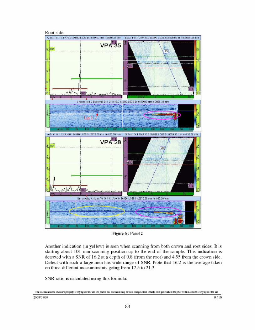
83
84
85
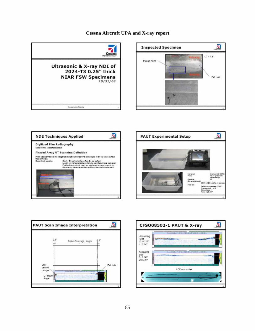
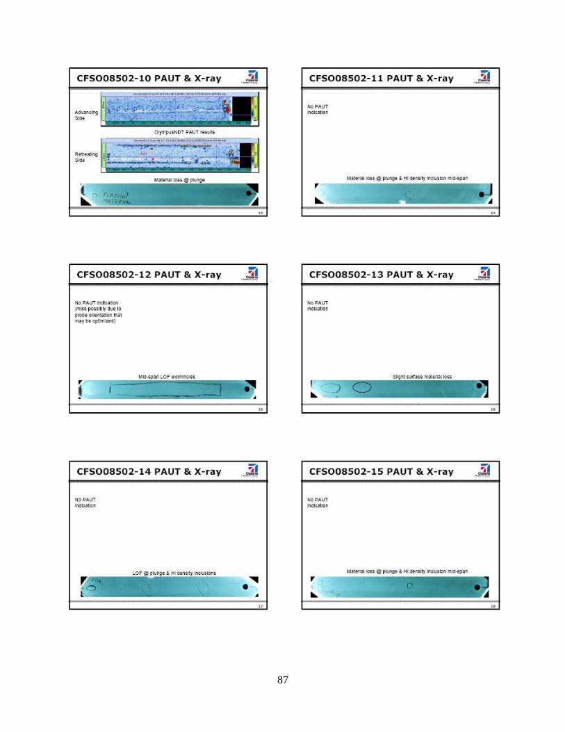
Cessna Aircraft UPA and X-ray report
86
87
88
89
90
91
Hawker Beechcraft X-ray Analysis Report
work order list 11/21/2008NDI analysis Hawkerbeechcraft Wes Timmerman Level 3
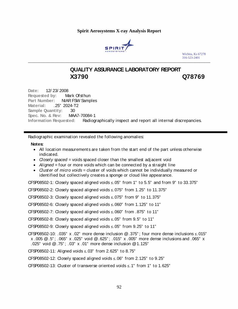
Radiographic examination revealed the following anomalies:
Notes: • All location measurements are taken from the start end of the part unless otherwise
indicated. • Closely spaced = voids spaced closer than the smallest adjacent void • Aligned = four or more voids which can be connected by a straight line • Cluster of micro voids = cluster of voids which cannot be individually measured or
identified but collectively creates a sponge or cloud like appearance.
CFSP08502-1: Closely spaced aligned voids ≤.05” from 1” to 5.5” and from 9” to 33.375”
CFSP08502-2: Closely spaced aligned voids ≤.075” from 1.25” to 11.375”
CFSP08502-3: Closely spaced aligned voids ≤.075” from 9” to 11.375”
CFSP08502-6: Closely spaced aligned voids ≤.060” from 1.125” to 11”
CFSP08502-7: Closely spaced aligned voids ≤.060” from .875” to 11”
CFSP08502-8: Closely spaced aligned voids ≤.05” from 9.5” to 11”
CFSP08502-9: Closely spaced aligned voids ≤.05” from 9.25” to 11”
CFSP08502-10: .035” x .02” more dense inclusion @ .375”; four more dense inclusions ≤.015” x .005 @ .5”; .065” x .025” void @ .625”; .015” x .005” more dense inclusions and .065” x .025” void @ .75”; .03” x .01” more dense inclusion @ 1.125”
CFSP08502-11: Aligned voids ≤.03” from 2.625” to 8.75”
CFSP08502-12: Closely spaced aligned voids ≤.06” from 2.125” to 9.25”
CFSP08502-13: Cluster of transverse oriented voids ≤.1” from 1” to 1.625”
Date: 12/23/2008 Requested by: Mark Ofsthun Part Number: NIAR FSW Samples Material: .25” 2024-T2 Sample Quantity: 30 Spec. No. & Rev: MAA7-70084-1 Information Requested: Radiographically inspect and report all internal discrepancies.
93
CFSP08502-14: .035” x .03” void @ 2.75”; seven more dense inclusions ≤.035” x .03” from 4.375” to 4.625”; .015” x .005” more dense inclusion @ 5.25”; .02” x .005” more dense inclusion @ 5.75”; 30+ more dense inclusions ≤.11” x .03” clustered at 8.375”
CFSP08502-15: .025” x .02” more dense inclusion @ 10.875”
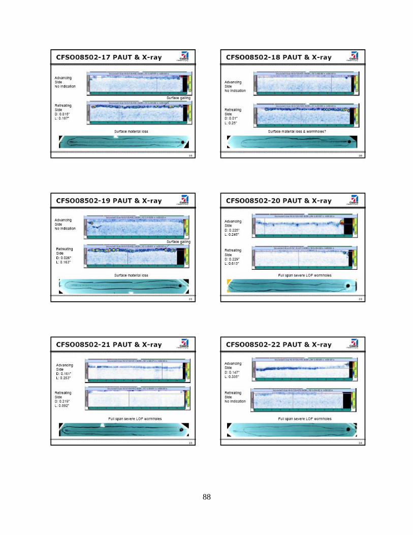
CFSP08502-17: Continuous band up to .225” in width of closely spaced voids from .875” to 11.25”, some of which are open to the surface
CFSP08502-18: Continuous band up to .225” in width of closely spaced voids from 1.375” to 11.25”, some of which are open to the surface
CFSP08502-19: Continuous band up to .25” in width of closely spaced voids from .5” to 11.375”, some of which are open to the surface
CFSP08502-20: Cluster of closely spaced voids, some of which are interconnected, beginning @ .5” continuing to 1.75” where the voids become a worm hole that continues to 11.25”
CFSP08502-21: Cluster of closely spaced voids, some of which are interconnected, beginning @ .5” continuing to 2.25” where the voids become a worm hole that continues to 11.25”
CFSP08502-22: Cluster of closely spaced voids, some of which are interconnected, beginning @ .5” continuing to 1.5” where the voids become a worm hole that continues to 11.25”
CFSP08502-23: Cluster of closely spaced voids, some of which are interconnected, beginning @ .625” continuing to 1.5” where the voids become a worm hole that continues to 7”, begins again @ 7.5” to 8.375, then from 8.625” to 10.125” and from 10.375” to 11.5”
CFSP08502-24: Cluster of voids ≤.075” from .375” to 1.5”; .02” wide worm hole from 2” to 2.625” and from 2.875” to 6.375” and from 6.625” to 7.375” and from 7.875” to 11.25”
CFSP08502-25: Cluster of voids ≤.125” from .375” to 1.1”; cluster of micro voids from .875” to 1.5”; worm hole from 1.25” to 1.625” and from 2.75” to 11.25”
CFSP08502-26: No anomalies detected
CFSP08502-27: No anomalies detected
CFSP08502-28: No anomalies detected
CFSP08502-29: Cluster of closely spaced voids ≤.10”, some of which are interconnected, beginning @ .5” continuing to 2.5” where the voids become a worm hole that continues to 11”; numerous clusters of micro voids from 1.25” to 10.375” some of which are open to the surface
CFSP08502-30: Cluster of closely spaced voids ≤.10”, some of which are interconnected, beginning @ .5” continuing to 2.75” where the voids become a worm hole that continues to 11”; large clusters of micro voids from .75” to 10.25” some of which are open to the surface
CFSP08502-32: Closely spaced aligned voids ≤.075”, some of which are interconnected, beginning at .5” continuing to 11”; clusters of micro voids from 1” to 3.25”
CFSP08502-33: Closely spaced aligned voids ≤.05” from 9.875” to 11.125”
CFSP08502-34: Closely spaced aligned voids ≤.05” from 10.375” to 11”
Inspection perform by: James M. Winter Date: 12/23/2008 Stamp: Level III
94
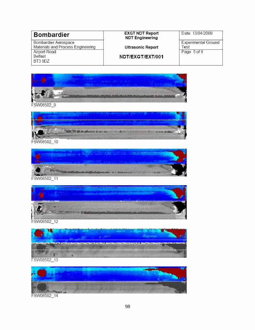
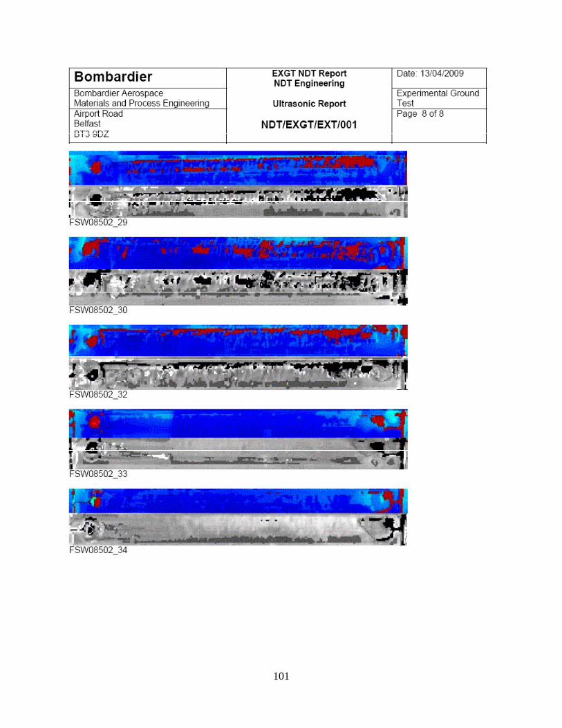
Learjet-Bombardier-Short Brothers X-ray and Ultrasonic Phased Array Analyses Report
95
96
97
98
99
100
101
102
Neural Network Classification- FSWAT
Just for the software: 1 is a good weld and 0 is a bad weld. Criterion:
• Classified as 1 means it is a good weld when actually it is a 0, a bad weld. It is a void not detected.
• 0 when it is 1, it is a good weld classified as bad. It is a false detection.
Neural network information <learning rate> <momentum> 0.25 0.25 <number of epochs> 500 Training data classification <total samples> <correctly classified> <% of correctness> 166 166 100% the average training error per sample is 4.7896e-005 the average test error per sample is 0.0291887 # misclassification: 171 - line No, 0.452481 - false class , actually 1 # misclassification: 185 - line No, 0.00783703 - false class , actually 1 # misclassification: 216 - line No, 0.9976 - false class , actually 0 # misclassification: 219 - line No, 0.808082 - false class , actually 0 # misclassification: 221 - line No, 0.104356 - false class , actually 1 # misclassification: 230 - line No, 0.610587 - false class , actually 0 Novel data classification <total samples> <correctly classified> <% of correctness> 83 77 92.7711%
103
Spirit Aerosystems X-ray Analysis on Tensile Coupons Report
CFSP08502-1-T1 Tightly spaced voids ≤.075” diameter across entire width of sampleCFSP08502-1-T3 Tightly spaced voids ≤.025” diameter across entire width of sampleCFSP08502-2-T1 Tightly spaced voids ≤.025” diameter across entire width of sampleCFSP08502-2-T2 Continuously connected voids across entire width of sampleCFSP08502-3-T4 Tightly spaced voids ≤.025” diameter across entire width of sampleCFSP08502-6-T1 Tightly spaced voids ≤.015” diameter across entire width of sampleCFSP08502-6-T2 Tightly spaced voids ≤.075” diameter across entire width of sampleCFSP08502-7-T1 Tightly spaced voids ≤.025” diameter across entire width of sampleCFSP08502-7-T2 Tightly spaced voids ≤.050” diameter across entire width of sampleCFSP08502-8-T4 Tightly spaced voids ≤.050” diameter across entire width of sampleCFSP08502-12-T1 Nine (9) voids ≤.050” diameter equally spaced across entire width of sampleCFSP08502-12-T2 Eight (8) voids ≤.050” diameter equally spaced across entire width of sampleCFSP08502-17-T1 Clusters up to .110” wide of minute pores across entire width of sampleCFSP08502-17-T2 Clusters up to .130” wide of minute pores across entire width of sampleCFSP08502-17-T3 Clusters up to .150” wide of minute pores across entire width of sampleCFSP08502-18-T1 Clusters up to .080” wide of minute pores across entire width of sampleCFSP08502-18-T2 Clusters up to .175” wide of minute pores across entire width of sampleCFSP08502-19-T1 Clusters up to .140” wide of minute pores across entire width of sampleCFSP08502-19-T2 Clusters up to .175” wide of minute pores across entire width of sampleCFSP08502-19-T3 Clusters up to .050” wide of minute pores across entire width of sampleCFSP08502-19-T4 Clusters up to .110” wide of minute pores across entire width of sampleCFSP08502-19-T5 Clusters up to .200” wide of minute pores across entire width of sampleCFSP08502-20-T1 Approximately .030” wide worm hole across entire width of sampleCFSP08502-20-T2 Approximately .030” wide worm hole across entire width of sampleCFSP08502-20-T3 Approximately .040” wide worm hole across entire width of sampleCFSP08502-20-T4 Approximately .050” wide worm hole across entire width of sampleCFSP08502-21-T1 Approximately .040” wide worm hole across entire width of sampleCFSP08502-21-T2 Approximately .030” wide worm hole across entire width of sampleCFSP08502-22-T1 Approximately .035” wide worm hole across entire width of sampleCFSP08502-22-T2 Approximately .035” wide worm hole across entire width of sampleCFSP08502-22-T3 Approximately .045” wide worm hole across entire width of sample
MAA7-70084-1Information Requested: Report all anomalies ≤.005” and mark samples
Requested by:Part Number:Material:
Spec. No. & Rev:
104
CFSP08502-23-T1 Approximately .010” wide worm hole across entire width of sampleCFSP08502-23-T2 Approximately .015” wide worm hole across entire width of sampleCFSP08502-23-T3 Approximately .005” wide worm hole across entire width of sampleCFSP08502-24-T1 Approximately .005” wide worm hole across entire width of sampleCFSP08502-24-T2 Approximately .010” wide worm hole across entire width of sampleCFSP08502-24-T3 Approximately .010” wide worm hole across entire width of sampleCFSP08502-24-T4 Approximately .010” wide worm hole across entire width of sampleCFSP08502-25-T2 Approximately .010” wide worm hole across entire width of sampleCFSP08502-29-T1 Approximately .025” wide worm hole across entire width of sampleCFSP08502-29-T2 Approximately .025” wide worm hole across entire width of sampleCFSP08502-30-T1 Approximately .025” wide worm hole across entire width of sampleCFSP08502-30-T2 Approximately .025” wide worm hole across entire width of sampleCFSP08502-30-T3 Approximately .030” wide worm hole across entire width of sample
CFSP08502-32-T
CFSP08502-32-T Approximately .025” wide worm hole across entire width of sample
CFSP08502-32-TApproximately twelve (12) voids ≤.025” diameter randomly dispersed across entire width of sample
Approximately fifteen (15) voids ≤.025” diameter randomly dispersed across entire width of sample