v2020 1 / 7 Biomathematics 2 Probability, random variables. Continuous random variable. Normal, standard normal distribution. Dr. Beáta Bugyi associate professor University of Pécs, Medical School Department of Biophysics 2020
Transcript
v2020
1 / 7
Biomathematics 2
Probability, random variables.
Continuous random variable. Normal, standard normal
distribution.
Dr. Beáta Bugyi
associate professor
University of Pécs, Medical School
Department of Biophysics
2020
v2020
2 / 7
CONTINUOUS RANDOM VARIABLE continuous: uncountable, infinite number of values, arises from measurement
Probability – discrete/continuous random variables
Let’s consider that a statistical experiment has an outcome corresponding to
A) a discrete random variable and X = 0 – 10 (finite number of outcomes: 10)
Give the probability that the outcome is 6.
𝑃(𝑋 = 6) =1
10= 0.1
B) a continuous random variable and X = 0 – 10 (infinite number of outcomes)
Give the probability that the outcome is 6. Exactly 6, not 6.1, 6.01, …, 6.00000000001
𝑃(𝑋 = 6) =1
∞= 0
NORMAL DISTRIBUTION
𝑁(𝜇, 𝜎), 𝜇 = 𝑚𝑒𝑎𝑛, 𝜎 = 𝑠𝑡𝑎𝑛𝑑𝑎𝑟𝑑 𝑑𝑒𝑣𝑖𝑎𝑡𝑖𝑜𝑛
Probability density function (PDF)
𝑓(𝑥) =1
√2𝜋𝜎2exp (−
(𝑥 − 𝜇)2
2𝜎2 )
Cumulative density function (CDF)
𝐹(𝑥) = ∫1
√2𝜋𝜎2exp (−
(𝑥 − 𝜇)2
2𝜎2 )𝑥
−∞
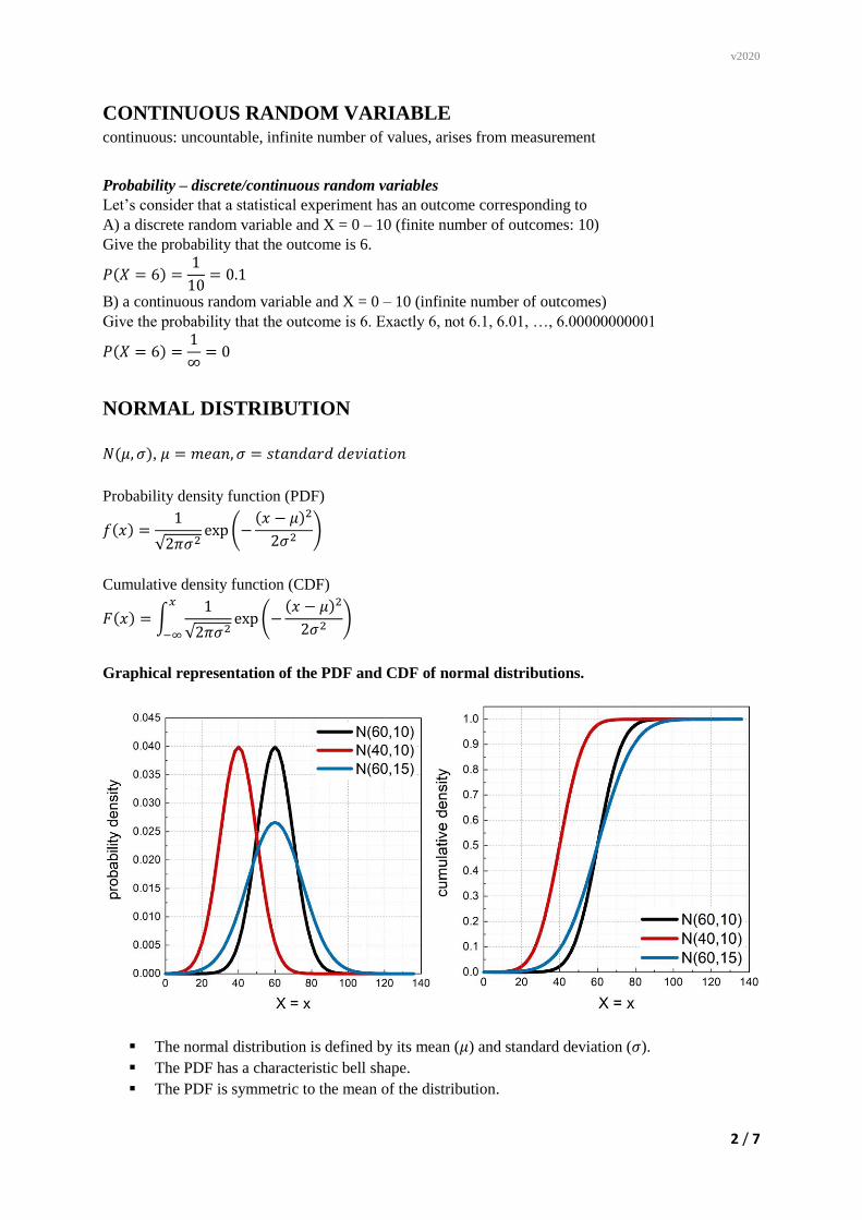
Graphical representation of the PDF and CDF of normal distributions.
The normal distribution is defined by its mean (𝜇) and standard deviation (𝜎).
The PDF has a characteristic bell shape.
The PDF is symmetric to the mean of the distribution.
v2020
3 / 7
The inflection point of the PDF corresponds to the standard deviation of the distribution.
The width (width at half-maximum) of the PDF is proportional to the standard deviation; the
larger the width the larger the standard deviation.
Probability is given by the area under the PDF (see examples below).
Example 1
The test result of students from Subject 1 follows a normal distribution with a mean of 60% and
standard deviation of 10%. 𝑵(𝝁, 𝝈) = 𝑵(𝟔𝟎, 𝟏𝟎). Represent graphically the following
probabilities.
Q1.1: What is the probability that a student scores 60%? 𝑃(𝑋 = 𝑥 = 60) = ?
Q1.2: What is the probability that a student scores less than 60%? 𝑃(𝑋 < 𝑥 = 60) =?
Q1.3: What is the probability that a student scores more than 60%? 𝑃(𝑋 > 𝑥 = 60) = ?
Q1.4: What is the probability that a student scores less than 80%? 𝑃(𝑋 < 𝑥 = 80) = ?
Q1.5: What is the probability that a student scores between 60% and 80%? 𝑃(𝑥 = 60 < 𝑋 < 𝑥 =
80) = ?
Example 2
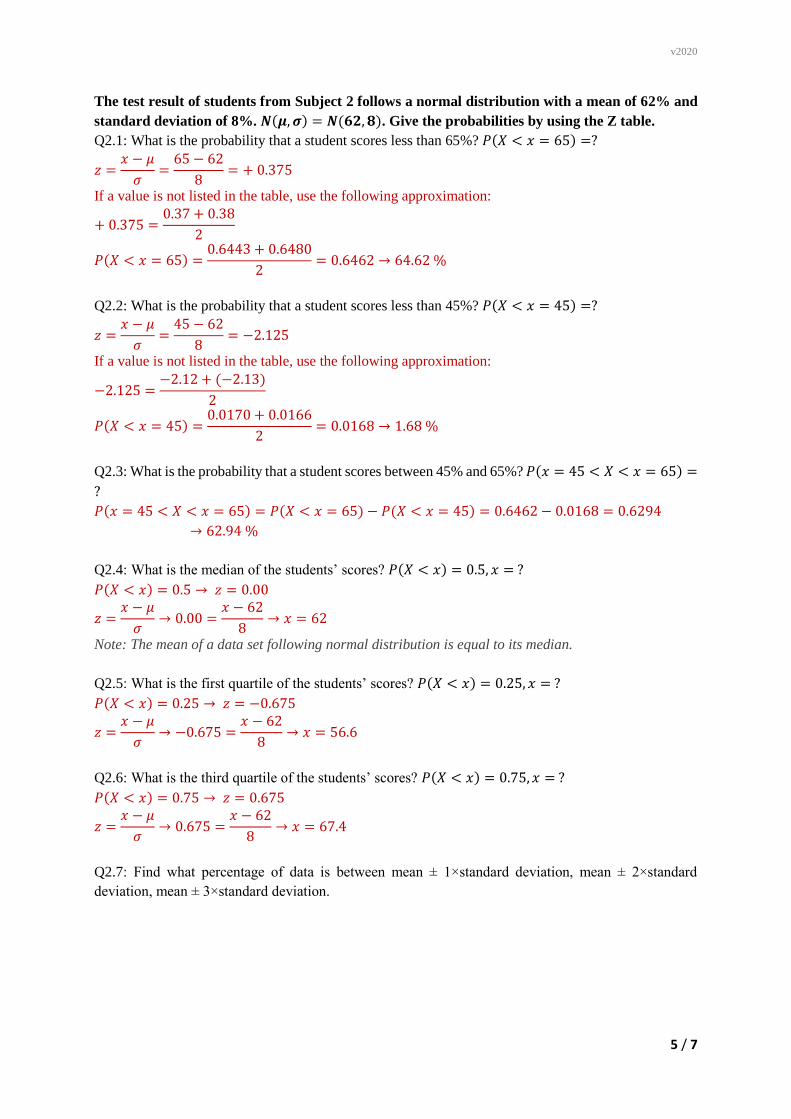
The test result of students from Subject 2 follows a normal distribution with a mean of 62% and
standard deviation of 8%. 𝑵(𝝁, 𝝈) = 𝑵(𝟔𝟐, 𝟖).
Question:
How can we work with different normal distributions? Do we need the PDF of each and every normal
distribution?
Answer:
Normal distributions can be standardized; ∞ normal distribution 1 standardized distribution
(standard normal distribution)
How to standardize normal distributions?
𝑁(𝜇, 𝜎)
z score: 𝒛 =𝒙−𝝁
𝝈
z score: how many standard deviations (𝜎) is a given value (𝑥) from the mean (𝜇)
STANDARD NORMAL DISTRIBUTION
𝑆𝑁(0, 1), 𝜇 = 1, 𝜎 = 0
Probability density function (PDF)
𝑓(𝑥) =1
√2𝜋𝜎2exp (−
(𝑥−𝜇)2
2𝜎2 ) , 𝑤ℎ𝑒𝑟𝑒 𝜇 = 0 𝑎𝑛𝑑 𝜎 = 1: 𝑓(𝑥) =1
√2𝜋exp (−
𝑥2
2),
Cumulative density function (CDF)
𝐹(𝑥) = ∫1
√2𝜋exp (−
𝑥2
2)
𝑥
−∞
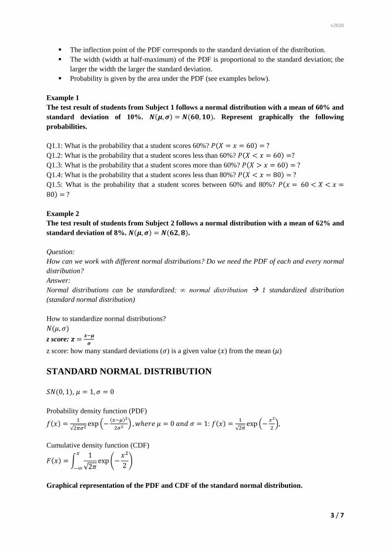
Graphical representation of the PDF and CDF of the standard normal distribution.
v2020
4 / 7
Z table
summarizes the CDF of the standard normal distribution
Example 1
The test result of students from Subject 1 follows a normal distribution with a mean of 60% and
standard deviation of 10%. 𝑵(𝝁, 𝝈) = 𝑵(𝟔𝟎, 𝟏𝟎). Standardize the normal distribution. Give the
probabilities by using the Z table.
Q1.1: What is the probability that a student scores 60%? 𝑃(𝑋 = 𝑥 = 60) = ?
𝑃(𝑋 = 𝑥 = 60) = 0
Q1.2: What is the probability that a student scores less than 60%? 𝑃(𝑋 < 𝑥 = 60) =?
𝑧 =𝑥 − 𝜇
𝜎=
60 − 60
10= 0.00
𝑃(𝑋 < 𝑥 = 60) = 0.5 → 50 %
Q1.3: What is the probability that a student scores more than 60%? 𝑃(𝑋 > 𝑥 = 60) = ?