Probing cosmological variation of the proton-to-electron ... · PDF fileProbing cosmological...

Probing cosmological variation of theproton-to-electron mass ratio by means

of quasar absorption spectra

Dissertation

zur Erlangung des Doktorgrades

des Department Physik

der Universitat Hamburg

vorgelegt von

Martin Wendt

aus Peine

Hamburg2010

Gutachter der Dissertation:Prof Dr. D. ReimersProf Dr. L. Wisotzki

Gutachter der Disputation:Prof Dr. J. H. M. M. SchmittProf Dr. P. H. Hauschildt

Prufungsausschussvorsitzender:Dr. R. Baade

Datum der Disputation:22.07.2010

“It is impossible for a manto learn

what he thinks

he already knows.”-Epictetus

Zusammenfassung

Die vorliegende Arbeit beschaftigt sich mit der Analyse einer moglichen Variationdes Proton-Elektron-Massenverhaltnisses und der dazu verwendeten Methodik.Die Analyse basiert auf Beobachtungsdaten von QSO 0347-383, einem hellenQuasar 17ter Große mit einer Rotverschiebung von z = 3.025. Sein Absorptions-spektrum weist H i-Systeme hoher Saulendichte und folglich teilweise gesattigteLinien mit ausgepragten Dampfungsflugeln auf. Ein beobachtetes DLA-Systemzeigt optisch dunne Absorptionslinien von molekularem Wasserstoff H2. EineVariation der dimensionslosen fundamentalen physikalischen Konstanten µ =mp/me ließe sich anhand der Lyman- und Werner-Ubergange bestimmen. Bisherwurden ledigich vier unterschiedliche Systeme mit teils widerspruchlichen Resul-taten zur Analyse herangezogen.

Die Ubergangsenergien verschiedener Rotations- und Vibrationsniveaus von H2

sind von der reduzierten Masse des Molekuls abhangig. Eine Abweichung vomLaborwert µ = 1836.15267261(85) (Mohr and Taylor 2005) kann anhand exakterVermessung entsprechender Absorptionslinien bestimmt werden. Die individu-ell gemessene Rotverschiebung jeder Linie ist der einzige relevante Parameterund beinhaltet zunachst die kosmologische Rotverschiebung des DLA-Absorbersund einen moglichen additiven Anteil aufgrund von Ubergangsenergien, die beigegebener Variation von den lokalen Energiedifferenzen der einzelnen Niveausabweichen.

Diese Arbeit bewertet die erreichbare Genauigkeit einer derartigen Bestimmungeiner Variation von µ und liefert fundierte Ergebnisse. Ziel ist es, bestehendeWiderspruche in den Resultaten unterschiedlicher Arbeitsgruppen aufzulosen undHinweise auf deren Ursachen auszuarbeiten. Dieses wird durch unterschiedlicheund voneinander unabhangige Ansatze bei der Analyse erreicht.

Der hohe Anspruch an Genauigkeit den dieses Forschungsfeld diktiert, machtes erforderlich, die einfließenden Fehlerquellen qualitativ und nach Moglichkeitquantitativ zu bestimmen. Ein wichtiges Kriterium sind reproduzierbare Ergeb-nisse, die die Messdaten einschließlich ihrer Streuung hinreichend beschreiben.Die gemeinsame Betrachtung zweier getrennt voneinander gewonnener Datensatzevon QSO 0347-383 ergibt: ∆µ/µ =

(

15 ± (9stat + 6sys))

× 10−6 bei zabs = 3.025.Die Genauigkeit der Messungen wird zu 300 m s−1 bestimmt, bestehend aus etwa180 m s−1 aufgrund von Fitfehlern und etwa 120 m s−1 systematischer Natur, ins-besondere der Wellenlangenkalibration.

Eine Analyse von Daten, die mit Hinsicht auf die besonderen Anspruche bei

der Bestimmung von ∆µ/µ in jungster Vergangenheit gewonnen wurden, liefert:∆µ/µ =

(

2.9 ± (6stat + 2sys))

× 10−6 fur eine Zeitspanne von ca. 12 Gyr. Diedeutlichere Einschrankung einer moglichen Variation von µ ist vor allem auf dieum Faktor zwei hohere Auflosung und die grundlichere Wellenlangenkalibrationder 2009 gewonnen Daten zuruckzufuhren.Bisher erfolgte Untersuchungen geben Anlass zur Annahme, dass systematischeFehler bislang generell unterschatzt wurden und die Ergebnisse somit beinflussten.Die vorliegende Arbeit verwirft die Hypothese einer Variation des Proton-Elektron-Massenverhaltnisses von mehr als 1 ppm und liefert alternative Herangehensweisenzur Fehlerbehandlung und -erkennung, die speziell in Hinblick auf zu erwartendeQualitat zukunftiger Daten von zunehmender Bedeutung sind.

Abstract

This thesis examines the methods and procedures involved in the determinationof a possible variation of the proton-electron mass ratio on cosmological timescales. The studied object QSO 0347-383 is a bright quasar of 17th magnitude ata redshift of z = 3.025. Its spectrum shows absorption systems of high H i columndensity leading to saturated absorption features with prominent damping wings.One of those DLA systems contains observable molecular hydrogen H2 apparentin optically thin absorption features. The variation of the dimensionless fun-damental physical constant µ = mp/me can be checked through observation ofLyman and Werner lines of molecular hydrogen observed in the spectra of distantQSOs. Only few, at present 4, systems have been used for the purpose providingdifferent results between the different authors.

The electro-vibro-rotational transitions of H2 depend differently on the reducedmass of the H2 molecule. A possible deviation from the local value of µ =1836.15267261(85) (Mohr and Taylor 2005) can be ascertained from exact mea-surements of the observed transitions. The required observable parameter is solelythe redshift. It includes the cosmological redshift of the DLA system and a pos-sible additive component rising from possible changes in the individual transitionfrequencies due to variation in the reduced mass of the molecule. This thesisassesses the accuracy of the investigation concerning a possible variation of µ andprovides robust results. The goal in mind is to resolve the current controversy onvariation of µ and devise explanations for the different findings. This is achievedby providing alternative approaches to the problem.

The demand for precision requires a deep understanding of the errors involved.Self-consistency in data analysis and effective techniques to handle unknown sys-tematic errors are essential. An analysis based on independent data sets ofQSO 0347-383 is put forward and new approaches for some of the steps in-volved in the data analysis are introduced. Drawing on two independent ob-servations of a single absorption system in QSO 0347-383 the detailed analysisyields ∆µ/µ =

(

15 ± (9stat + 6sys))

× 10−6 at zabs = 3.025. Based on the overallgoodness-of-fit the limit of accuracy is estimated to be ∼ 300 m s−1, consisting ofroughly 180 m s−1due to the uncertainty of the fit and about 120 m s−1allocatedto systematics.

Utilizing very recent data observed in 2009 and dedicated to the subject of chang-ing fundamental constants of the same system with twice the resolving power,the result on µ is constrained to ∆µ/µ =

(

2.9 ± (6stat + 2sys))

× 10−6 for a look

back time of ∼ 12 Gyrs. Current contradictory findings tend to underestimatethe impact of systematic errors. This work presents alternative approaches tohandle systematics and introduces new methods required for precision analysis ofQSO spectra available now and within the foreseeable future.Altogether, no indication for variation of µ is found. The new constraint on thetime dependence of the proton-to-electron mass ratio reached by this work issubstantiated by following different approaches.

Contents

1 Introduction 1

2 Background 4

2.1 Cosmology of varying fundamental constants . . . . . . . . . . . . 42.1.1 Accessible constants . . . . . . . . . . . . . . . . . . . . . 8

2.2 Observables . . . . . . . . . . . . . . . . . . . . . . . . . . . . . . 102.2.1 Proton-to-electron mass ratio µ . . . . . . . . . . . . . . . 102.2.2 Intergalactic H2 . . . . . . . . . . . . . . . . . . . . . . . . 102.2.3 Laboratory wavelengths . . . . . . . . . . . . . . . . . . . 132.2.4 Sensitivity coefficients Ki . . . . . . . . . . . . . . . . . . . 142.2.5 Status quo for ∆µ/µ . . . . . . . . . . . . . . . . . . . . . 16

3 Analysis I 20

3.1 Data . . . . . . . . . . . . . . . . . . . . . . . . . . . . . . . . . . 203.1.1 QSO 0347-383 . . . . . . . . . . . . . . . . . . . . . . . . . 203.1.2 Reduction . . . . . . . . . . . . . . . . . . . . . . . . . . . 22

3.2 Preprocessing of data . . . . . . . . . . . . . . . . . . . . . . . . . 243.2.1 Conditioning of flux . . . . . . . . . . . . . . . . . . . . . 243.2.2 Correction for individual shifts . . . . . . . . . . . . . . . . 243.2.3 Selection of H2 lines . . . . . . . . . . . . . . . . . . . . . 28

3.3 Fitting . . . . . . . . . . . . . . . . . . . . . . . . . . . . . . . . . 343.3.1 Simultaneous fit vs. co-added fit . . . . . . . . . . . . . . . 363.3.2 Continuum handling . . . . . . . . . . . . . . . . . . . . . 37

4 Results I 40

4.1 Determination of ∆µ/µ . . . . . . . . . . . . . . . . . . . . . . . . 404.2 Result via discrete line pairs . . . . . . . . . . . . . . . . . . . . . 45

5 Error Analysis I 48

5.1 Quality of fit . . . . . . . . . . . . . . . . . . . . . . . . . . . . . 485.2 Standard Error . . . . . . . . . . . . . . . . . . . . . . . . . . . . 505.3 Uncertainties in the sensitivity coefficients . . . . . . . . . . . . . 515.4 Influence analysis of data preprocessing . . . . . . . . . . . . . . . 535.5 Rotational Levels - medium dependent . . . . . . . . . . . . . . . 545.6 Vibrational Levels - energy dependent . . . . . . . . . . . . . . . . 56

5.7 Electronic levels - Lyman, Werner bands . . . . . . . . . . . . . . 585.8 Accuracy of line fits . . . . . . . . . . . . . . . . . . . . . . . . . . 60

6 Analysis II 64

6.1 Data . . . . . . . . . . . . . . . . . . . . . . . . . . . . . . . . . . 646.1.1 2009 observations . . . . . . . . . . . . . . . . . . . . . . . 646.1.2 Reduction . . . . . . . . . . . . . . . . . . . . . . . . . . . 67

6.2 Preprocessing of data . . . . . . . . . . . . . . . . . . . . . . . . . 706.2.1 Correction for individual shifts . . . . . . . . . . . . . . . . 706.2.2 Selection of H2 lines . . . . . . . . . . . . . . . . . . . . . 706.2.3 Resolution . . . . . . . . . . . . . . . . . . . . . . . . . . . 73

7 Results II 76

7.1 Determination of ∆µ/µ . . . . . . . . . . . . . . . . . . . . . . . . 767.2 Result via discrete line pairs . . . . . . . . . . . . . . . . . . . . . 80

8 Error Analysis II 82

8.1 Impact of wavelength calibration issues . . . . . . . . . . . . . . . 828.2 Test for correlation of redshift and photon energy . . . . . . . . . 848.3 Variability of QSO 0347-383 . . . . . . . . . . . . . . . . . . . . . 858.4 Calibration and positioning errors . . . . . . . . . . . . . . . . . . 87

9 Conclusions 90

9.1 Inference on cosmology . . . . . . . . . . . . . . . . . . . . . . . . 909.2 Outlook . . . . . . . . . . . . . . . . . . . . . . . . . . . . . . . . 93

Overview of written Programs 96

List of Figures 99

List of Tables 101

Acknowledgements 103

References 105

Erklarung 117

1 Introduction

The Standard Model of particle physics (SMPP) is very successful and its predic-tions are tested to high precision in laboratories around the world. SMPP needsseveral dimensionless fundamental constants, such as coupling constants and massratios, whose values cannot be predicted and must be established through exper-iment (Fritzsch 2009). Our confidence in their constancy stems from laboratoryexperiments over human time-scales but variations might have occurred over the14 billion-year history of the Universe while remaining undetectably small today.

The possible variation of the fundamental constants of nature is currently a verypopular research topic and has a long history (Dirac 1937; Gamow 1967) Theo-ries unifying gravity and other interactions suggest the possibility of spatial andtemporal variation of physical “constants” in the Universe (see, e.g. Marciano1984; Uzan 2003). Current interest is high because in superstring theories –which have additional dimensions compactified on tiny scales – any variation ofthe size of the extra dimensions results in changes in the 3-dimensional couplingconstants. At present no mechanism for keeping the spatial scale static has beenfound (e.g., our three “large” spatial dimensions increase in size). Moreover, thereexists a mechanism for making all coupling constants and masses of elementaryparticles both space and time dependent, and influenced by local circumstances(see, e.g., Uzan 2003). The variation of coupling constants can be non-monotonic(e.g., damped oscillations). Indeed, in theoretical models seeking to unify the fourforces of nature, the coupling constants vary naturally on cosmological scales. Theproton-to-electron mass ratio, µ = mp/me has been the subject of numerous stud-ies. The mass ratio is sensitive primarily to the quantum chromodynamic scale.The ΛQCD scale should vary considerably faster than that of quantum electro-dynamics ΛQED. As a consequence, the secular change in the proton-to-electronmass ratio, if any, should be larger than that of the fine structure constant. Thismakes µ a very interesting target to search for possible cosmological variationsof the fundamental constants. The present value of the proton-to-electron massratio is µ = 1836.15267261(85) (Mohr and Taylor 2005). Laboratory experimentsby comparing the rates between clocks based on hyperfine transitions in atomswith a different dependence on µ restrict the time-dependence of µ at the levelof (µ/µ)t0 = (1.6 ± 1.7) × 10−15 yr−1 (Blatt et al. 2008).

A probe of the variation of µ is obtained by comparing rotational versus vibra-tional modes of molecules as first suggested by Thompson (1975). The methodis based on the fact that the wavelengths of vibro-rotational lines of molecules

2 CHAPTER 1. INTRODUCTION

depend on the reduced mass, M, of the molecule. The energy difference betweentwo consecutive levels of the rotational spectrum of a diatomic molecule scale asM, whereas the energy difference between two adjacent levels of the vibrationalspectrum is proportional to M−1/2:

ν ∼ celec +cvib

µ1/2+

crot

µ. (1.1)

Consequently, by studying the Lyman and Werner transitions of molecular hy-drogen we may obtain information about a change in µ. The observed wavelengthλ of any given line in an absorption system at the redshift z differs from the lo-cal rest-frame wavelength λ0 of the same line in the laboratory according to therelation

λ = λ0(1 + z)

(

1 + K∆µ

µ

)

(1.2)

where K is the sensitivity coefficient computed theoretically for the Lyman andWerner bands of the H2 molecule. Using this expression, the cosmological redshiftof a line can be distinguished from the shift due to a variation of µ.This method was used to obtain upper bounds on the secular variation of theproton-to-electron mass ratio from observations of distant absorption systems inthe spectra of quasars at several redshifts. The quasar absorption system towardsQSO 0347-383 was first studied using high-resolution spectra obtained with theVery Large Telescope/Ultraviolet-Visual Echelle Spectrograph (VLT/UVES). Afirst stringent bound was derived at (−1.8± 3.8)× 10−5 (Levshakov et al. 2002).Subsequent measures of the quasar absorption systems of QSO 0347-382 andQSO 1232+082 provided hints for a variation at 3.5 σ (Reinhold et al. 2006;Ivanchik et al. 2005; Ubachs et al. 2007):

∆µ/µ = (2.4 ± 0.6) × 10−5. (1.3)

The new analysis used additional high-resolution spectra and updated laboratorydata of the energy levels and of the rest frame wavelengths of the H2 molecule.However, more recently King et al. (2008); Wendt and Reimers (2008) and Thomp-son et al. (2009a) re-evaluated data of the same system and report a result inagreement with no variation. The most stringent limits on ∆µ/µ have been re-ported at ∆µ/µ = (2.6 ± 3.0stat) × 10−6 from the combination of three H2 systems(King et al. 2008) and a fourth one has provided (+5.6 ± 5.5stat ± 2.7sys) × 10−6

(Malec et al. 2010).In this work, the same data of QSO 0347-383 that led in parts to the abovementioned results is analyzed in combination with supplemental observationscarried out independently at the same time by another group. This utilizationof previously overlooked data enables an improved analysis of the systematicsinvolved and increases the total signal-to-noise ratio notably.

3

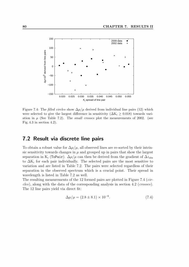
The corresponding analysis and its detailed error handling are described in chap-ter Analysis I on page 20 and following pages. The present analysis is motivatedon one side by the use of a new data set available in the ESO data archive and pre-viously overlooked and on the other side by numerous findings of different groupsthat partially are in disagreement with each other. A large part of these dis-crepancies reflect the different methods of handling systematic errors. Evidentlysystematics are not yet under control or fully understood. This work emphasizesthe importance to take these errors, in particular calibration issues, into accountand put forward some measures adapted to the problem.The second part of this thesis deals with the latest observations in the field of vari-ation in fundamental physical constants. Recorded at UVES/VLT in September2009, the telescope setup during observations and the following data reductionwere carried out with the needs for highest precision in mind. The obtained datais of high-quality and its detailed analysis yields the most stringent constraint on∆µ for a single absorber. The methods involved in the determination of µ andthe refinements in the data analysis are illustrated in chapter Analysis II onpage 64 and following pages.The bounds on the variation of µ are generally obtained by using the vibro-rotational transitions of molecular hydrogen, since H2 is a very abundant moleculealthough very rarely seen in quasar absorber. Very few studies used other moleculessince they are difficult to detect and measure accurately at large redshifts. Ingeneral these methods provide less stringent bounds for high redshifts. This the-sis will concentrate on the single H2 system observed towards QSO 0347-383 totrace the proton-to-electron mass ration µ at high redshift (zabs = 3.025). Thiswork reaches a robust estimation of the achievable accuracy with current data bycomparing independent observation runs and the latest available data.

2 Background

2.1 Cosmology of varying fundamental constants

The development of physics relied considerably on the Copernican principle,which states that the Earth is not in a central, specially favored position in theuniverse and that the laws of physics do not differ from one point in spacetimeto another. In cosmology, if one assumes the Copernican principle and observesthat the universe appears isotropic from our vantage-point on Earth, then onecan prove that the Universe is generally homogeneous (at any given time) andis also isotropic about any given point. These two conditions comprise the cos-mological principle. It is however natural to question this assumption. It isdifficult to imagine a change of the form of physical laws but a smooth changein the physical constants is much easier to conceive. Comparing and reproducingexperiments is also a root of the scientific approach which makes sense only ifthe laws of nature do not depend on time and space. This hypothesis of con-stancy of the constants plays an important role in particular in astronomy andcosmology where the redshift measures the look-back-time. Ignoring the possi-bility of varying fundamental physical constants could lead to a distorted view ofour universe and if such a variation is established corrections would have to beapplied. It is thus of great importance to investigate this possibility especially asthe measurements become more and more precise.

Evidently, the constants have not undergone huge variations on Solar systemscales and geological time scales and one is looking for tiny effects. The questionof the numerical values of fundamental physical constants is central to physicsand one can hope to explain them dynamically as predicted by some high-energytheories. Testing the constancy of the constants is part of the tests of generalrelativity.This speculative theory which embeds varying constants is analogous to the tran-sition from the Newtonian description of mechanics in which space and time werejust a static background in which matter was evolving to the relativistic descrip-tion where spacetime becomes a dynamical quantity determined by the Einsteinequations (Damour 2001).

There are several reasons why the possibility of varying constants should be takenseriously. First, we know that the best candidates for unification of the forces ofnature in a quantum gravitational environment only seem to exist in finite form ifthere are many more dimensions of space than the three that we are familiar with.

2.1. COSMOLOGY OF VARYING FUNDAMENTAL CONSTANTS 5

This means that the true constants of nature are defined in higher dimensionsand the three-dimensional projections we observe are no longer fundamental anddo not need to be constant. Any slow change in the scale of the extra dimensionswould be revealed by measurable changes in our three-dimensional ‘constants’.Second, we appreciate that some apparent constant might be determined partiallyor completely by spontaneous symmetry-breaking processes in the very earlyuniverse.This introduces an irreducibly random element into the values of those constants.They may be different in different parts of the universe and hence at differentdirections or different redshifts. The most dramatic manifestation of this processis provided by the chaotic and eternal inflationary universe scenarios where boththe number and the strength of forces in the universe at low energy can fallout differently in different regions. Third, any outcome of a theory of quantumgravity will be intrinsically probabilistic. It is often imagined that the probabilitydistributions for observables will be very sharply peaked but this may not be thecase for all possibilities. Thus, the value of the gravitation ‘constant’, G, or itstime derivative, G, might be predicted to be spatial random variables. Fourth, anon-uniqueness of the vacuum state for the universe would allow other numericalcombinations of the constants to have occurred in different places. String theoryindicates that there is a huge ‘landscape’ (> 10500) of possible vacuum states thatthe universe can find itself residing in as it expand and cools (Barrow 2005). Eachwill have different constants and associated forces and symmetries. It is soberingto remember that at present we have no idea why any of the natural constantstake the numerical values they do and we have never successfully predicted thevalue of any dimensionless constant in advance of its measurement.A fist step is to evaluate which physical constants are to be considered in general.Levy-Leblond (1977) defined three classes of fundamental constants, since not allconstants of physics play the same role:

• The class A of the constants characteristic of particular objects,• The class B of the constants characteristic of a class of physical phenomena,• The class C being the class of universal constants.

This definition of a fundamental constant, however, can cause the change of statusof constants, as can be exemplified by the constant c, the speed of light. Initiallybeing a type A constant (describing a property of light), then becoming a typeB constant when it was realized that it was related to the electro-magnetic phe-nomena and it ended as type C constant (it is part of many laws of physics fromelectromagnetism to relativity). It has even become a much more fundamentalconstant since it has been chosen as the new definition of the meter (see Petley1983).A more conservative definition of a fundamental constant would thus be to statethat it is any parameter that can not be calculated with our present knowledge

6 CHAPTER 2. BACKGROUND

of physics, e.g. a free parameter of our theory at hand. Each free parameter ofany theory is in fact a challenge for future theories to explain the value (Uzan2003).

The set of constants which are conventionally considered as fundamental consistsof the electron charge e, the electron mass me, the proton mass mp, the reducedPlanck constant ~, the velocity of light in vacuum c, the Avogadro constantN

A, the Boltzmann constant k

B, the Newton constant G, the permeability and

permittivity of space, ε0 and µ0. The latter has a fixed value in the SI systemof unit (µ0 = 4π × 10−7 H m−1) which is implicit in the definition of the Ampere;ε0 is then fixed by the relation ε0µ0 = c−2. To compare with, the minimalstandard model of particle physics plus gravitation that describes the four knowninteractions depends on 20 free parameters (Cahn 1996; Hogan 2000): the Yukawacoefficients determining the masses of the six quark (u, d, c, s, t, b) and three lepton(e, µ, τ) flavors, the Higgs mass and vacuum expectation value, three angles and aphase of the Cabibbo-Kobayashi-Maskawa matrix, a phase for the QCD vacuumand three coupling constants g

S, g

W, g1 for the gauge group SU(3)×SU(2)×U(1)

respectively. Below the Z mass, g1 and gW

combine to form the electro-magneticcoupling constant.

The final number of free parameters indeed depends on the physical model athand (see, e.g., Weinberg 1983). The introduction of constants in physical law isclosely related to the existence of systems of units. Newton’s law states that thegravitational force between two masses is proportional to each mass and inverselyproportional to their separation. To transform the proportionality to an equalityone requires the use of a quantity with dimension of m3kg−1s−2 independentof the separation between the two bodies, of their mass, of their composition(equivalence principle) and on the position (local position invariance). Withanother system of units this constant could have simply been anything.

The determination of the laboratory value of constants relies mainly on the mea-surements of lengths, frequencies, times,... (see Flowers and Petley 2001). Hence,any question on the variation of constants is linked to the definition of the systemof units and to the theory of measurement. The choice of a base units affects thepossible time variation of constants.

The behavior of atomic matter is mainly determined by the value of the electronmass and of the fine structure constant. The Rydberg energy sets the (non-relativistic) atomic levels, the hyperfine structure involves higher powers of thefine structure constant, and molecular modes (including vibrational, rotationalmodes) depend on the mass ratio mp/me. As a consequence, if the fine structureconstant is spacetime dependent, the comparison between several devices suchas clocks and rulers will also be spacetime dependent. This dependence willalso differ from one clock to another so that metrology becomes both device andspacetime dependent.

Besides this first metrologic problem, the choice of units has implications on the


permissible variations of certain dimensionful constant. Petley (1983) discussesthe implication of the definition of the meter for example. The original definitionof the meter via a prototype platinum-iridium bar depends on the interatomicspacing in the material used in the construction of the bar. Atkinson (1968)argued that, at first order, it mainly depends on the Bohr radius of the atom sothat this definition of the meter fixes the combination (2.12) as constant. Anotherdefinition was based on the wavelength of the orange radiation from krypton-86atoms. It is likely that this wavelength depends on the Rydberg constant andon the reduced mass of the atom so that it ensures that mec

2α2EM

/2~ is constant.The more recent definition of the meter as the length of the path traveled by lightin vacuum during a time of 1/299, 792, 458 of a second imposes the constancy ofthe speed of light1 c. Identically, the definitions of the second as the duration of9,192,631,770 periods of the transition between two hyperfine levels of the groundstate of cesium-133 or of the kilogram via an international prototype respectivelyimpose that m2

ec2α4

EM/~ and mp are fixed.

Since the definition of a system of units and the value of the fundamental con-stants (and thus the status of their constancy) are entangled, and since the mea-surement of any dimensionful quantity is in fact the measurements of a ratioto standards chosen as units, it only makes sense to consider the variation ofdimensionless ratios.

The required approach is to focus on the variation of dimensionless ratios which,for instance, characterize the relative magnitude of two forces, and are indepen-dent of the choice of the system of units and of the choice of standard rulers orclocks.

Notations: In this work, SI units and the following values of the fundamentalconstants today2 are used:

c = 299, 792, 458 ms−1 (2.1)

~ = 1.054571596(82)× 10−34 Js (2.2)

G = 6.673(10) × 10−11 m3kg−1s−2 (2.3)

me = 9.10938188(72)× 10−31 kg (2.4)

mp = 1.67262158(13)× 10−27 kg (2.5)

mn = 1.67492716(13)× 10−27 kg (2.6)

e = 1.602176462(63)× 10−29 C (2.7)

for the velocity of light, the reduced Planck constant, the Newton constant, themasses of the electron, proton and neutron, and the charge of the electron.

1Note that the velocity of light is not assigned a fixed value directly, but rather the value isfixed as a consequence of the definition of the meter.

2see http://physics.nist.gov/cuu/Constants/ for an up to date list of the recommendedvalues of the constants of nature.


Defined as well are

q2 ≡ e2

4πε0

, (2.8)

and the following dimensionless ratios

αEM

≡ q2

~c∼ 1/137.03599976(50) (2.9)

µ ≡ mp

me

∼ 1836.15267247(80). (2.10)

(2.11)

The notations

a0 =~

mecαEM

= 0.5291771 A (2.12)

−EI =1

2mec

2α2EM

= 13.60580 eV (2.13)

R∞ = −EI

hc= 1.0973731568549(83)× 107 m−1 (2.14)

respectively for the Bohr radius, the hydrogen ionization energy and the Rydbergconstant are introduced.Note, in some works µ is referred to as electron-to-proton mass ratio me/mp,which has the effect of a change in sign for ∆µ/µ. The cited values in this thesisare converted accordingly.

2.1.1 Accessible constants

A prominent fundamental constant that meets the above mentioned requirementsis the proto-to-electron mass ratio µ =mp/me (see Eq. 2.10). The time variationof µ is given by:

µ

µ=

mp

mp− me

me. (2.15)

Though the proton mass mp depends not only on the quantum chromodynamics(QCD) scale ΛQCD but also on the masses of the up quark and the down quark,mp is usually considered to be proportional to ΛQCD since these quark masses aremuch smaller than ΛQCD.The fine-structure constant α (see Eq. 2.9) is not taken into account here but hasproven to be another suiteable fundamental physical constant. For an atom/ion,the relativistic corrections to the energy levels of an electron are proportionalto α2, although the magnitude of the change depends on the transition underconsideration. The tests for variation in µ and α run completely independentfrom each other but most theories suggest a certain correlation between the two.The fine-structure constant is hence mentioned since early observations gave rise


to this rich field of varying constants and the efforts in constraining both α andµ stand to benefit from each other.Theoretically there is a wide range of possible connections between the fine-structure constant α and the proton-to-electron mass ratio µ. In numerous con-sidered models variations in α lead to variations in the electron mass (via theelectron self-energy) and in the proton mass (via the electrostatic energy con-tained inside a proton). These are model dependent and in general quite complexto work out (see, e.g., Dine et al. 2003).The first observational indications of potential variation stimulated numeroustheoretical works to explain the new findings. An often-cited paper3 on α is theone by Webb et al. (2001), which reports:

∆α

α= (−0.72 ± 0.18) × 10−5, (2.16)

Or later, a paper on α by Murphy et al. (2003):

∆α

α= (−0.543 ± 0.116) × 10−5, (2.17)

though similar observations of other groups did not necessarily reproduce thatresult. Observations of Reinhold et al. (2006) suggested a fractional change inthe proton-to-electron mass ratio µ =mp/me:

∆µ

µ= (2.4 ± 0.6) × 10−5, (2.18)

for a weighted fit to observations at a redshift of z ∼ 3, which implies that theproton-to-electron mass ratio has decreased over the last 12Gyr. These two ex-tremes among the different findings were taken as boundary conditions for a largerange of theoretical works, since from the theoretical point of view, it is naturalto allow time and space dependence of fundamental constants. In fact, super-string theory, which is expected to unify all fundamental interactions, predictsthe existence of a scalar partner φ (called dilaton) of the tensor graviton, whose ex-pectation value determines the string coupling constant gs = eφ/2 (Witten 1984).The couplings of the dilaton to matter induces the violation of the equivalenceprinciple and hence generates deviations from general relativity. With the abovementioned observational results, the hints of the time variation of fundamentalconstants were considered to be found (see, e.g., Calmet and Fritzsch 2006; Chibaet al. 2007).The following section will specify the modus operandi and the necessary require-ments to measure the proton-to-electron mass ratio on cosmological scales.

3More than 430 citations to this day.


2.2 Observables

2.2.1 Proton-to-electron mass ratio µ

As first pointed out by Thompson (1975) molecular absorption lines can providea test of the variation of µ. The energy difference between two adjacent rotationallevels in a diatomic molecule is proportional to Mr−2, r being the bond length andM the reduced mass, and that the vibrational transition of the same molecule has,in first approximation, a

√M dependence. For molecular hydrogen M = mp/2

so that comparison of an observed vibro-rotational spectrum with its presentanalog will thus give information on the variation of mp and mn. Comparingpure rotational transitions with electronic transitions gives a measurement of µ.Following Thompson (1975), the frequency of vibration-rotation transitions is, inthe Born-Oppenheimer approximation, of the form

ν ∼ EI (celec

+ cvib

/√

µ + crot

/µ) (2.19)

where celec

, cvib

and crot

are some numerical coefficients. Comparing the ratioof wavelengths of various electronic-vibration-rotational lines in quasar spectrumand in the laboratory allow to trace the variation of µ since, at lowest order,Eq. (2.19) implies

∆Eij(z)

∆Eij(0)= 1 + Kij

∆µ

µ+ O

(

∆µ2

µ2

)

, (2.20)

where the coefficients Kij determine the sensitivity of the transition energies toa change in µ. An important point is that the values of Kij differ for differentlines. Thus, if the reduced mass of a molecule at the epoch z differs from thepresent value, then the observered wavelength and the corresponding sensitivitycoefficient Kij of that transition must be linearly correlated. This implicit cor-relation underlies the method. Section 2.2.4 describes how these coefficients canbe computed.

2.2.2 Intergalactic H2

Molecular hydrogen H2 is the most abundant molecule in the universe and plays afundamental role in many astrophysical contexts. It is found in all regions wherethe shielding of the ultraviolet photons, responsible for the photo-dissociationof H2, is sufficiently large. Except in the early universe, most H2 is thoughtto be produced via surface reactions on interstellar dust grains, since gas-phasereactions are too slow in general (see, e.g., Habart et al. 2004).The H2 formation mechanism is not yet fully understood. Direct observations ofH2 are difficult since electronic transitions occur only in the ultraviolet to whichEarth’s atmosphere is opaque. UV satellites are only suited for bright nearby

2.2. OBSERVABLES 11

objects and could not provide the necessary resolution. Only at great distancesand hence with a large redshift these spectra are shifted into the visual bandand can then be observed with ground-based telescopes. Another problem is thenarrow range of conditions under which H2 forms. The required dust grains thatallow for the forming of molecular hydrogen can easily obscure the molecularhydrogen as well.Hydrogen makes up about 80% of the known matter in the universe and most of itis contained in either atomic or molecular hydrogen in the gaseous phase (Combesand Pineau Des Forets 2000). It took until 1970 for the first detection of molecularhydrogen in space; the observation was made possible through the use of a rocketborne spectrometer observing from high altitudes, therewith evading atmosphericabsorption of the vacuum ultraviolet radiation. Lyman bands in the wavelengthrange between 1000 and 1100 A were identified in the absorption spectrum of adiffuse interstellar cloud in the optical path towards ξ Persei (Carruthers 1970).Further satellite based observations also revealed absorption of Werner bands andUV emission of Lyman and Werner bands including their continua (Spitzer et al.1974). The Copernicus satellite telescope greatly improved the possibilities forrecording UV-spectra of molecular hydrogen (see, e.g., Morton and Dinerstein1976).The International Ultraviolet Explorer (IUE), launched January 1978 and in ser-vice until September 1996, covered ultraviolet wavelengths from 1200 to 3350 Awith two on-board spectrographs. It detected for example vibrationally excitedmolecular hydrogen in the upper atmosphere of Jupiter (Cravens 1987).The new Far Ultraviolet Spectroscopic Explorer (FUSE), in flight between June1999 and october 2007, is an ideally suited spectroscopic measurement device toprobe hydrogen in space. It covers the wavelength range 905-1187 A, the rangeof the strong Lyman and Werner absorption bands, with high resolution and itis now used routinely for H2 observations (Moos et al. 2000).For this thesis, publicly available FUSE data was widely used to verify line listsof vibro-rotational transitions and to test the written graphical data examina-tion (GRADE4) tool against. However, its data unfortunately cannot be used forlocal space based measurements of µ since the FUSE satellite bears no on boardcalibration set up. Instead the obtained spectra are calibrated via the observedH2 absorption features.The abundance of molecular hydrogen in space is usually expressed as the fractionf(H2) ≡ 2N(H2)/[2N(H2) + N(H i)].Savage et al. (1977) found the correlation for H2 in our galaxy:

f(H2) ≥ 10−2 for N(H i) > 4 × 1020 cm−2. (2.21)

A threshold of 5 A for the equivalent width in the search for DLA systems, asmentioned above, corresponds to N(H i) ≥ 2 × 1020 cm−2 and thus a fraction of

4see Appendix for a short summary of programs written in the course of this thesis.


Table 2.1: List of damped Lyman-α systems with H2 absorption observations

Quasar source redshift zabs

QSO 0515-441 1.15QSO 1331+170 1.78QSO 0551-336 1.96QSO 0013-004 1.97QSO 1444+014 2.09QSO 1232+082 2.34QSO 2343+125 2.43QSO 0405-443 2.59QSO 0528-250 2.81QSO 0347-383 3.02QSO 0000-263 3.39QSO 1443-272 4.22

f(H2) > 10−2 cm−2 would be expected for most of the DLA systems. Albeit theobserved f(H2) in distant DLA is much lower than that. The low H2 content inDLA in contrast to our galaxy is likely due to their comparably low dust contents.The fraction of molecular Hydrogen can be described as the ratio of its formationon dust grains and its photodissociation by UV-photons via f(H2) = 2Rn/Iwhere I is proportional to the intensity of UV radiation and R is proportional tothe dust-to-gas ratio κ. A low f(H2) in DLAs could then be attributed to a lowdust content, and thus a low κ. Such a correlation was indeed found by Petitjeanet al. (2002).

Long before the actual observation of molecular hydrogen, Herzberg had discussedthe possibility of detecting H2 in outer space through the quadrupole spectrum,even before these very weak features were observed in the laboratory (Herzberg1949). With the further development of infrared sensitive CCD cameras, the 2 µminfrared emissions, coinciding with an atmospheric transmission window, couldbe mapped in 2D-imaging pictures of distributions of hot molecular hydrogen inspace (Field et al. 1994).

Levshakov and Varshalovich (1985) tentatively assigned some features in spectraobtained by Morton et al. (1980) from PKS 0528-250 (one of the few systems upto date used for determination of µ). Similar spectra of this system were collectedby Foltz et al. (1988) and this data formed the basis for a constraint on a possiblevariation of µ put forward by Varshalovich and Levshakov (1993).

Further reports on observation of molecular hydrogen absorption lines at highredshift are given by Ge and Bechtold (1997) at z = 1.97 towards QSO 0013-004,by Reimers et al. (2003) at z = 1.15 towards QSO 0515-441, and by Cui et al.(2005) at z = 1.78 towards QSO 1331+170. Observations by the VLT/UVES

2.2. OBSERVABLES 13

instrument led to H2 detection towards QSO 0347-383, QSO 1232+082 (Ivanchiket al. 2002; Levshakov et al. 2002) and towards QSO 0551-336 (Ledoux et al.2002).

Additional observations of H2 are reported towards Q 0000-263 in Levshakovet al. (2000). Ledoux et al. (2003) and Srianand et al. (2005) performed surveys onDamped Lyman-a (DLA) systems at redshifts z > 1.8, in which some new quasarswith H2 absorption were detected. From their study and from past searches theyconclude that molecular hydrogen is detected in 13 − 20% of the systems.

More recently Petitjean et al. (2006) observed the systems QSO 2343+125 andQSO 2348-011, while Ledoux et al. (2006) observed H2 lines in a source at thehighest redshift until now (z = 4.22).

The observations of 2006 and the continued survey for DLAs demonstrate thatthe amount of known H2 absorbing clouds at high redshift is rapidly expanding;it is therefore likely that additional high resolution data to extract informationon µ variation will become available in the near future. Noterdaeme et al. (2008)at all conclude from the comparison between H2-bearing systems and the overallUVES sample, that a significant increase of the molecular fraction in DLAs couldtake place at redshifts zabs ≥ 1.8. The known DLA systems with H2 absorptionare listed in Table 2.1.

2.2.3 Laboratory wavelengths

For some time the only available precise data on oscillator frequencies and forthis study more important rest frame wavelengths for molecular hydrogen werethose computed by Abgrall et al. (1993a). The claimed accuracy lay at about1m A corresponding to ∼ 4 mA for the observer’s frame in this case. This is onthe order of the by now reached accuracy in line fits and improvements in thedetermination of the restframe wavelength was mandatory.

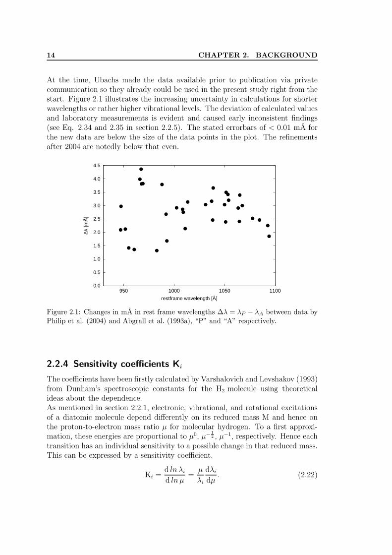
Philip et al. (2004) eventually conducted high-resolution laser-spectroscopy togain precise transition frequencies in the Lyman and Werner bands via directmeasurements. A strong test on the accuracy of transition frequencies is to com-pare the differences between the rotational branches P (J + 2) and R(J). Theyshould match the calculated ground state rotational splittings, which are accu-rately known (see Jennings et al. 1984). The achieved accuracy is stated as< 0.01 mA. In the framework of this analysis the rest frame wavelength can thusbe assumed to be exact. Due to experimental restrictions on the UV laser rangethe transition frequencies were obtained only for a subset of the lines detected inthe spectrum of QSO 0347-383. As can be seen in Figure 2.1 the new data has athroughout positive varying offset, which strongly influences ∆µ/µ analysis.

More recent measurements (Hollenstein et al. 2006; Ivanov et al. 2008; Salumbideset al. 2008; Bailly et al. 2010) completed the data on the Lyman and Wernerband frequencies. The new data tables include all observed and selected H2 lines.


At the time, Ubachs made the data available prior to publication via privatecommunication so they already could be used in the present study right from thestart. Figure 2.1 illustrates the increasing uncertainty in calculations for shorterwavelengths or rather higher vibrational levels. The deviation of calculated valuesand laboratory measurements is evident and caused early inconsistent findings(see Eq. 2.34 and 2.35 in section 2.2.5). The stated errorbars of < 0.01 mA forthe new data are below the size of the data points in the plot. The refinementsafter 2004 are notedly below that even.

0.0

0.5

1.0

1.5

2.0

2.5

3.0

3.5

4.0

4.5

950 1000 1050 1100

∆λ [m

Å]

restframe wavelength [Å]

Figure 2.1: Changes in mA in rest frame wavelengths ∆λ = λP − λA between data byPhilip et al. (2004) and Abgrall et al. (1993a), “P” and “A” respectively.

2.2.4 Sensitivity coefficients Ki

The coefficients have been firstly calculated by Varshalovich and Levshakov (1993)from Dunham’s spectroscopic constants for the H2 molecule using theoreticalideas about the dependence.As mentioned in section 2.2.1, electronic, vibrational, and rotational excitationsof a diatomic molecule depend differently on its reduced mass M and hence onthe proton-to-electron mass ratio µ for molecular hydrogen. To a first approxi-mation, these energies are proportional to µ0, µ−

12 , µ−1, respectively. Hence each

transition has an individual sensitivity to a possible change in that reduced mass.This can be expressed by a sensitivity coefficient.

Ki =d ln λi

d ln µ=

µ

λi

dλi

dµ. (2.22)

2.2. OBSERVABLES 15

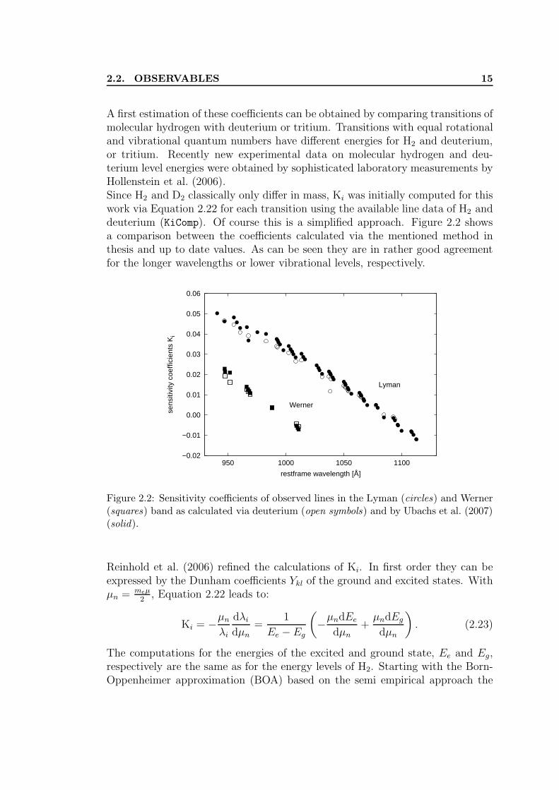
A first estimation of these coefficients can be obtained by comparing transitions ofmolecular hydrogen with deuterium or tritium. Transitions with equal rotationaland vibrational quantum numbers have different energies for H2 and deuterium,or tritium. Recently new experimental data on molecular hydrogen and deu-terium level energies were obtained by sophisticated laboratory measurements byHollenstein et al. (2006).Since H2 and D2 classically only differ in mass, Ki was initially computed for thiswork via Equation 2.22 for each transition using the available line data of H2 anddeuterium (KiComp). Of course this is a simplified approach. Figure 2.2 showsa comparison between the coefficients calculated via the mentioned method inthesis and up to date values. As can be seen they are in rather good agreementfor the longer wavelengths or lower vibrational levels, respectively.

−0.02

−0.01

0.00

0.01

0.02

0.03

0.04

0.05

0.06

950 1000 1050 1100

sens

itivi

ty c

oeffi

cien

ts K

i


Lyman

Werner

Figure 2.2: Sensitivity coefficients of observed lines in the Lyman (circles) and Werner(squares) band as calculated via deuterium (open symbols) and by Ubachs et al. (2007)(solid).

Reinhold et al. (2006) refined the calculations of Ki. In first order they can beexpressed by the Dunham coefficients Ykl of the ground and excited states. Withµn = meµ

2, Equation 2.22 leads to:

Ki = −µn

λi

dλi

dµn=

1

Ee − Eg

(

−µndEe

dµn+

µndEg

dµn

)

. (2.23)

The computations for the energies of the excited and ground state, Ee and Eg,respectively are the same as for the energy levels of H2. Starting with the Born-Oppenheimer approximation (BOA) based on the semi empirical approach the


energy levels can be expressed by the Dunham formula (see Dunham 1932):

E(v, J) =∑

k,l

Ykl

(

v +1

2

)k

[J(J +1)−Λ2]l; Λ2 =

0 for Lyman

1 for Werner(2.24)

However, the Dunham coefficients Ykl cannot be calculated directly from the levelenergies due to strong mutual interaction between the excited states as well asavoided rotational transitions between nearby vibrational levels. For the firsttime the more complex non-BOA effects are taken into account in Reinhold et al.(2006).

Ubachs et al. (2007) further improved the accuracy of sensitivity coefficients withlaboratory measurements of the level energies of molecular hydrogen via XUV-laser experiments allowed for a reliable enhancement of the BOA approximation.The Dunham coefficients Ykl for the lower states were fitted via experimental data.In general the sensitivity coefficients are largest at the shortest wavelengths (seeFigure 2.2), for both the Lyman and Werner systems. This is explained from thehigh vibrational quantum numbers associated with those lines. Further it canbe noted that for each band system at the long wavelength side the Ki valuesbecome negative. This is due to the larger zero-point vibrational energy in theground state than in the excited states.

Assessing the accuracy of these sensitivities proves to be very difficult. Ubachset al. (2007) estimate the overall uncertainty to be within 5 × 10−4, which cor-responds to 1% of the full range of Ki values (between -0.01 and 0.05). A moreprofund test can be accomplished though. Almost simultaneous to the efforts byReinhold et al. (2006), ab initio calculations of the sensitivity coefficients werecarried out by Meshkov et al. (2006). The differences between the coefficientsfrom the semi-empirical analysis (KSE), and the completely independent values(KAI) from ab initio analysis are plotted is Figure 2.3. All deviations ∆K liewithin margins of −2×10−4 and +4×10−4, corresponding to less than 1% of therange that the Ki values exhibit. In view of the entirely independent approachesto the problem this comparison produces some confidence in the correctness ofthe derived values. The plot however indicates systematic deviations for theWerner band (open circles) and a general increase in disagreement for the lowervibrational levels. At the current situation the estimated errors in the sensitivitycoefficients have no impact on the final result as shown in section 5.3.

2.2.5 Status quo for ∆µ/µ

Varshalovich and Levshakov (1993) used the observations of a damped Lyman-α system associated with the quasar PKS 0528-250 of redshift z = 2.811 anddeduced that

|∆µ/µ| < 4 × 10−3. (2.25)

2.2. OBSERVABLES 17

−2

−1

0

1

2

3

4

950 1000 1050 1100

∆K ×

104


Figure 2.3: Differences ∆K = KSE - KAI between derived K coefficients of the semi-empirical approach (Ubachs et al. 2007) and those of the ab initio calculation inMeshkov et al. (2006) for the Lyman (solid) and Werner (open) band.

A similar analysis was first tried by Foltz et al. (1988) but their work did not takeinto account the wavelength-to-mass sensitivity and their result hence seems notvery reliable. Nevertheless, they concluded that for z = 2.811:

|∆µ/µ| < 2 × 10−4. (2.26)

Cowie and Songaila (1995) observed the same quasar and deduced that

∆µ/µ = (−0.75 ± 6.25) × 10−4, (2.27)

at 95% C.L. from the data on 19 absorption lines.Varshalovich and Potekhin (1995) calculated the coefficient Kij to a higher pre-cision and deduced that

|∆µ/µ| < 2 × 10−4. (2.28)

Thereinafter, Varshalovich et al. (1996) used 59 transitions for H2 rotational levelsin PKS 0528-250 and got

∆µ/µ = (10 ± 12) × 10−5, (2.29)

at 2 σ level.These results were confirmed by Potekhin et al. (1998) using 83 absorption linesto get

∆µ/µ = (7.5 ± 9.5) × 10−5, (2.30)


at a 2 σ level.Later, Ivanchik et al. (2001) measured, with the VLT, the vibro-rotational lines ofmolecular hydrogen for two quasars with damped Lyman-α systems respectivelyat z = 2.3377 and z = 3.0249 and also argued for the detection of a time variationof µ. Their most conservative result is (the observational data were compared totwo experimental data sets)

∆µ/µ = (5.7 ± 3.8) × 10−5, (2.31)

at 1.5 σ and the authors cautiously point out that additional measurements arenecessary to ascertain this conclusion. The result is also dependent on the lab-oratory dataset of transition frequencies used for the comparison since it gave∆µ/µ = (12.2 ± 7.3) × 10−5 with another dataset.As in the case of Webb et al. (2001, 1999), indicating a detected variation in α

EM,

this measurement is very important in the sense that it is a non-zero detectionthat will have to be compared with other bounds. The measurements by Ivanchiket al. (2001) is indeed much larger than one would expect from the electromagneticcontributions. As seen in section 2.1 for any unified theory the changes in themasses are expected to be larger than the change in α

EM. Typically, we expect

∆µ/µ ∼ ∆ΛQCD

/ΛQCD

− ∆v/v ∼ (30 − 40)∆αEM

/αEM

, so that it seems that thedetection by Webb et al. (2001) is too large by an order of magnitude to becompatible with it (Uzan 2003).Levshakov et al. (2002) identified more than 80 H2 molecular lines in a dampedLyα (DLA) system at zabs = 3.025 toward QSO 0347-383. Due to H i Lyα forestcontamination several were considered unsuitable for further analysis and a subsetof 15 lines were chosen to set an upper limit on possible changes of µ:

|∆µ/µ| < 5.7 × 10−5. (2.32)

Ivanchik et al. (2003) find for QSO 0347-383:

∆µ/µ = (5.02 ± 1.82) × 10−5. (2.33)

In general the given errors represent the statistical errors alone. Which becomesevident in the follow up investigations of the same system:Based on the wavelengths given by Abgrall et al. (1993a,b) Ivanchik et al. (2005)find:

∆µ/µ = (3.05 ± 0.75) × 10−5, (2.34)

or, using new laboratory measurements by Philip et al. (2004) for wavelengthsdata:

∆µ/µ = (1.65 ± 0.74) × 10−5, (2.35)

and eventually the result by Reinhold et al. (2006):

∆µ/µ = (2.4 ± 0.6) × 10−5. (2.36)

2.2. OBSERVABLES 19

For the sake of completeness it should be noted, that Pagel (1983) used anothermethod to constrain µ based on the measurement of the mass shift in the spectrallines of heavy elements. In that case the mass of the nucleus can be consideredas infinite contrary to the case of hydrogen. A variation of µ will thus influencethe redshift determined from hydrogen. He compared the redshifts obtained fromspectrum of hydrogen atom and metal lines for quasars of redshift ranging from2.1 to 2.7. Since

∆z ≡ zH− z

metal= (1 + z)

∆µ

1 − µ0, (2.37)

he obtained that|∆µ/µ| < 4 × 10−1, (2.38)

at 3 σ level. This result is unfortunately not conclusive because usually heavyelements and hydrogen belong to different interstellar clouds with different radialvelocity.Apparently the laboratory measurements of µ itself were refined over the sameperiod as Figure 2.4 illustrates.

1836.15266

1836.15267

1836.15268

1836.15269

1836.15270

1836.15271

1836.15272

1836.15273

1980 1985 1990 1995 2000 2005 2010

prot

on−

to−

elec

tron

mas

s ra

tio µ

year

Cohen and Taylor 1986Mohr and Taylor 2000Mohr and Taylor 2005

Figure 2.4: Measurements of the proton-to-electron mass ratio, representing the valuesfor µ listed by the National Institute of Standards and Technology (NIST).

3 Analysis I

3.1 Data

3.1.1 QSO 0347-383

The source of the analysed spectrum is a bright quasi-stellar radio object (QSO)with a visual magnitude of V = 17.3 mag at a redshift of z = 3.23 (Maoz et al.1993), which shows a Damped Lyman α system (DLA) at zabs = 3.0245. Thehydrogen column density is N(H I)= 5 × 1020 cm−2 with a rich absorption-linespectrum (Levshakov et al. 2002). The DLA exhibits a multicomponent velocitystructure. There are at least two gas components: warm gas seen in lines ofneutral atoms, H and low ions, and hot gas where the resonance doublets ofC IV and Si IV are formed. In the cooler component molecular hydrogen wasfirst detected by Levshakov et al. (2002) who identified 88 H2 lines. First High-resolution spectra of the quasar QSO 0347-383 were obtained with the Ultraviolet-Visual Echelle Spectrograph (UVES) during commissioning at the Very LargeTelescope (VLT) 8.2m ESO telescope by D’Odorico et al. (2001). QSO 0347-383 is the identifier of the “Fundamental-Katalog 4.0” calibrated to 1950 butstill being widely used. The precise position dated to 2000 as stated in the fifthfundamental catalogue is α = 03h 49m 43.68s, δ = -3810′ 31.3′′.QSO 0347-383 itself was discovered by Osmer and Smith (1980). For the presentanalysis two independent data sets are taken into account. This first one wasalready described by Ivanchik et al. (2005) and Wendt and Reimers (2008). TheQuasar absorption line spectra were obtained with the UVES spectrograph atthe Very Large Telescope (VLT) of the European Southern Observatory (ESO)in Paranal, Chile. The slit was 0.8 arcsec wide resulting in a spectral resolutionof R ∼ 53.000 over the wavelength range 3300 A– 4500 A.The average seeing during observation was about 1.2 arcsec. Before and afterthe exposures for each night, Thorium-Argon calibration data were taken. Anoverall of 9 spectra were recorded with an exposure time of 4500 seconds eachbetween January 8th and January 10th 2002 for the ESO program 68.A-0106(A).All spectra were taken with grating with a central wavelength of 4303 A andthe blue “Pavarotti”-CCD with 2 × 2 binning. Later on the data were reducedmanually by Mirka Dessauges-Zavadsky from Geneva Observatory in Jan 2004 toachieve maximum accuracy. The ESO Ambient Conditions Database1 includes

1http://archive.eso.org/eso/ambient-database.html

3.1. DATA 21

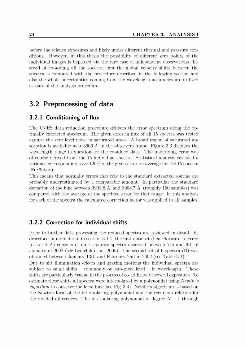
measurements of the environmental parameters at the Paranal ESO observatoryand shows no significant changes in temperatures during or in between the ex-posures that could lead to shifts between the separate observations. All works

Figure 3.1: Colour inverted and contrast enhanced photograph taken in the Blue-Band(J) covering a 14′ × 14′ area. QSO 0347-383 is marked by a circle and arrow. Originalimage from Space Telescope Science Institute (STScI).

on QSO 0347-383 are based on the same above mentioned UVES VLT observa-tions2 in January 2002 (see Ivanchik et al. 2005). The data used by Ivanchikwere retrieved from the VLT archive along with the MIDAS based UVES piplinereduction procedures.Additional observational data of QSO 0347-383 acquired in 2002 at the sametelescope but not previously analyzed3 is taken into account here.Paolo Molaro from the Osservatorio Astronomico di Trieste carefully reduced theoverlooked dataset again to meet present requirements and provided the data foranalysis.The UVES observations comprised of 6 × 80 minutes-exposures of QSO 0347-383on several nights, thus adding another 28.800 sec of exposure time. The journalof these observations as well as additional information is reported in Table 3.1.Three UVES spectra were taken with the DIC1 and setting 390+580 nm andthree spectra with DIC2 and setting 437+860, thus providing blue spectral rangesbetween 320-450 and 373-500 nm respectively. The spectrum of QSO 0347-383has no flux below 3700 A due to the Lyman discontinuity of the zabs=3.023absorption system. The slit width was set to 1′′ for all observations providing a

2Program ID 68.A-0106.3Program ID 68.B-0115(A).

22 CHAPTER 3. ANALYSIS I

Table 3.1: Journal of the observations

Date Time λ Exp(sec) Seeing (arcsec) airmass S/N (mean)

2002-01-13 03:42:54 390 4800 1.7 1.5 202002-01-14 02:13:24 390 4800 1.0 1.2 282002-01-15 00:43:32 437 4800 0.96 1.0 672002-01-18 03:25:04 437 4800 1.63 1.4 492002-01-24 02:20:14 437 4800 1.07 1.7 292002-02-02 01:33:58 390 4800 0.5 1.2 37

Resolving Power of ∼ 40.000. The seeing was varying in the range between 0.5′′

to 1.4′′ as measured by DIMM but normally seeing at the telescope is better thanthe value given by DIMM. The CCD pixels were binned by 2×2 providing aneffective 0.027-0.030 A pixel, or 2.25 kms−1 at 4000 A along dispersion direction.

0

5

10

15

20

3800 3900 4000 4100 4200 4300 4400

flux

a.u.

observed wavelength [Å]

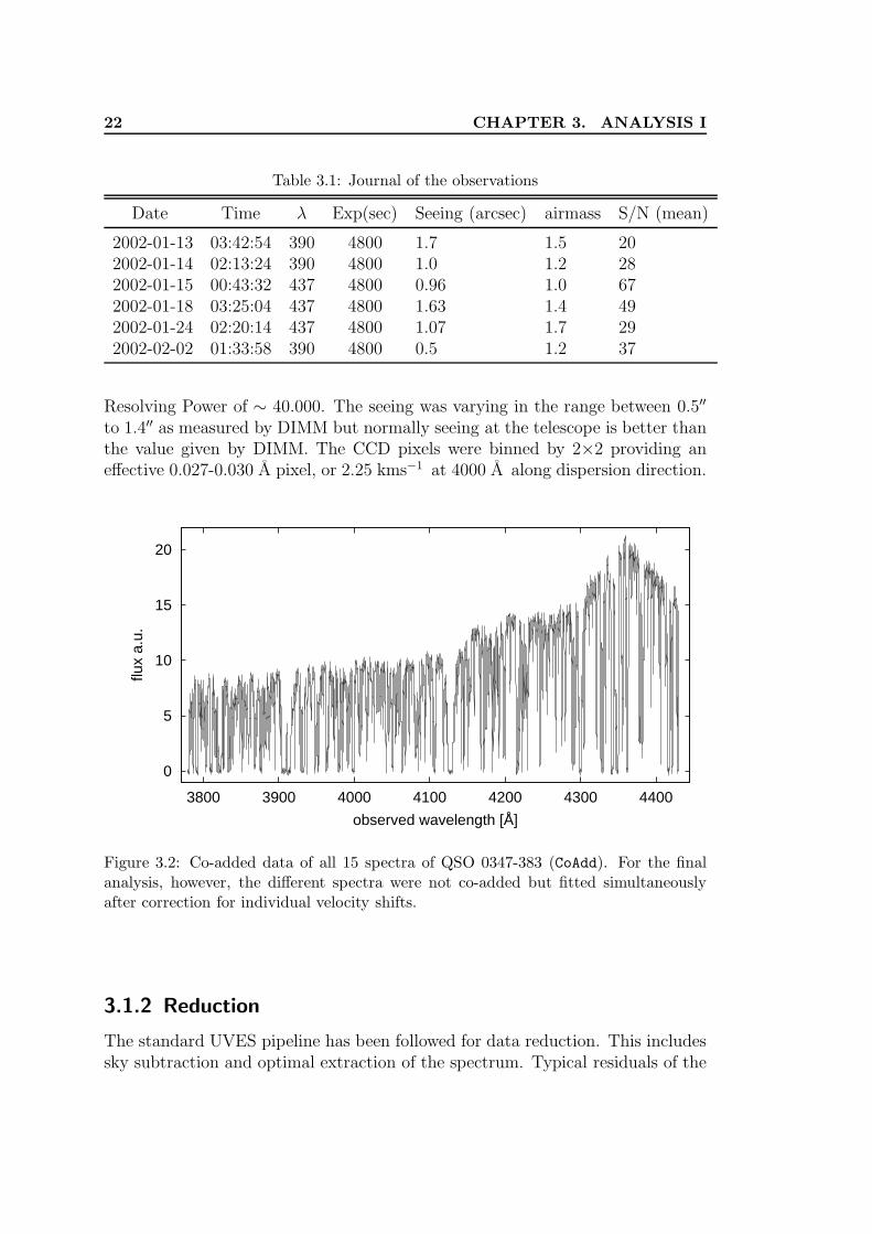
Figure 3.2: Co-added data of all 15 spectra of QSO 0347-383 (CoAdd). For the finalanalysis, however, the different spectra were not co-added but fitted simultaneouslyafter correction for individual velocity shifts.

3.1.2 Reduction

The standard UVES pipeline has been followed for data reduction. This includessky subtraction and optimal extraction of the spectrum. Typical residuals of the

3.1. DATA 23

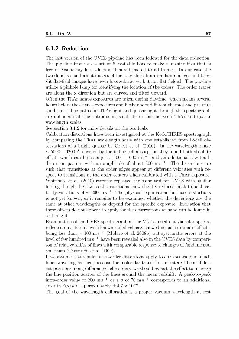
wavelength calibration were of ∼ 0.5 mA or ∼ 40 m s−1 at 4000 A. The spectrawere reduced to barycentric coordinates and air wavelengths have been trans-formed to vacuum by means of the dispersion formula given by Edlen (1966).Proper calibration and data reduction will be the key to detailed analysis of po-tential variations of fundamental constants. The influence of calibration issueson the data quality is hard to measure and the magnitude of the resulting sys-tematic error is under discussion. The measurements rely on detecting a patternof small relative wavelength shifts between different transitions spread through-out the spectrum. Normally, quasar spectra are calibrated by comparison withspectra of a hollow cathode thorium lamp rich in unresolved spectral lines. How-ever several factors are affecting the quality of the wavelength scale. The pathsfor ThAr light and quasar light through the spectrograph are not identical thusintroducing small distortions between ThAr and quasar wavelength scales. Inparticular differences in the slit illuminations are not traced by the calibrationlamp. Since source centering into the slit is varying from one exposure to anotheran offset in the zero point of the scales of different frames is induced which couldbe up to few hundred of m s−1. In section 3.2.2 an estimate of these offsets whichresult in a mean offset of 168 m s−1 are provided as well as a procedure to avoidthis problem. Laboratory wavelengths are known with limited precision which isvarying from line to line from about 15 m s−1 for the better known lines to morethan 100 m s−1 for the more poorly known lines (Murphy et al. 2008; Thomp-son et al. 2009a). However, this is the error which is reflected in the size of theresiduals of the wavelength calibration.

Effects of this kind have been investigated at the Keck/HIRES spectrograph bycomparing the ThAr wavelength scale with one established from I2-cell observa-tions of a bright quasar by Griest et al. (2010). They found both absolute andrelative wavelength offsets in the Keck data reduction pipeline which can be aslarge as 500 - 1000 m s−1for the observed wavelength range. Such errors wouldcorrespond to ∆λ ∼ 10− 20 mA and exceed by one order of magnitude presentlyquoted errors (Thompson et al. 2009a). Examination of the UVES spectrographat the VLT carried out via solar spectra reflected on asteroids with known radialvelocity showed no such dramatic offsets being less than ∼ 100 m s−1(Molaro et al.2008a) but systematic errors at the level of few hundred m s−1 have been revealedalso in the UVES data by comparison of relative shifts of lines with comparableresponse to changes of fundamental constants (Centurion et al. 2009). These ex-amples well show that current ∆µ/µ-analysis based on quasar absorption spectraat the level of a few ppm enters the regime of calibration induced systematicerrors. While awaiting a new generation of laser-comb-frequency calibration, to-day’s efforts to investigate potential variation of fundamental physical constantsrequire true consideration of the strong systematics.

The additional observations considered here were originally taken for other pur-poses and the ThAr lamps are taken during daytime, which means several hours


before the science exposures and likely under different thermal and pressure con-ditions. However, in this thesis the possibility of different zero points of theindividual images is bypassed via the rare case of independent observations. In-stead of co-adding all the spectra, first the global velocity shifts between thespectra is computed with the procedure described in the following section andalso the whole uncertainties coming from the wavelength accuracies are utilizedas part of the analysis procedure.

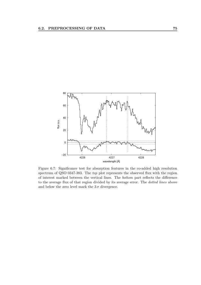
3.2 Preprocessing of data

3.2.1 Conditioning of flux

The UVES data reduction procedure delivers the error spectrum along the op-timally extracted spectrum. The given error in flux of all 15 spectra was testedagainst the zero level noise in saturated areas. A broad region of saturated ab-sorption is available near 3906 A in the observers frame. Figure 3.3 displays thewavelength range in question for the co-added data. The underlying error wasof course derived from the 15 individual spectra. Statistical analysis revealed avariance corresponding to ∼ 120% of the given error on average for the 15 spectra(ErrMeter).

This means that normally errors that rely to the standard extracted routine areprobably underestimated by a comparable amount. In particular the standarddeviation of the flux between 3903.8 A and 3908.7 A (roughly 160 samples) wascompared with the average of the specified error for that range. In this analysisfor each of the spectra the calculated correction factor was applied to all samples.

3.2.2 Correction for individual shifts

Prior to further data processing the reduced spectra are reviewed in detail. Esdescribed in more detail in section 3.1.1, the first data set (henceforward referredto as set A) consists of nine separate spectra observed between 7th and 9th ofJanuary in 2002 (see Ivanchik et al. 2005). The second set of 6 spectra (B) wasobtained between January 13th and February 2nd in 2002 (see Table 3.1).

Due to slit illumination effects and grating motions the individual spectra aresubject to small shifts – commonly on sub-pixel level – in wavelength. Theseshifts are particularly crucial in the process of co-addition of several exposures. Toestimate these shifts all spectra were interpolated by a polynomial using Neville’salgorithm to conserve the local flux (see Fig. 3.4). Neville’s algorithm is based onthe Newton form of the interpolating polynomial and the recursion relation forthe divided differences. The interpolating polynomial of degree N − 1 through

3.2. PREPROCESSING OF DATA 25

0

2

4

6

8

10

3898 3900 3902 3904 3906 3908 3910

flux

a.u.


saturated

Figure 3.3: Range of saturated absorption in the spectrum of QSO 0347-383 that canbe utilized to determine the minimal present gaussian error of the data. Plotted forthe co-added data for illustration purposes.

the N points y0 = f(x0), y1 = f(x1), . . . , yN−1 = f(xN−1) is given by Lagrange’sclassical formula,

P (x) =(x − x1)(x − x2) . . . (x − xN−1)

(x0 − x1)(x0 − x2) . . . (x0 − xN−1)y0

+(x − x1)(x − x2) . . . (x − xN−1)

(x1 − x0)(x1 − x2) . . . (x1 − xN−1)y1 + . . .

+(x − x1)(x − x2) . . . (x − xN−1)

(xN−1 − x0)(xN−1 − x1) . . . (xN−1 − xN−2)yN−1.

(3.1)

There are N terms, each a polynomial of degree N − 1 and each constructed tobe zero at all of the xi except one, at which it is constructed to be yi. Instead ofimplementing the Lagrange formula directly, Neville’s algorithm was used whichproceeds by first fitting a polynomial of degree 0 through the point (xk, yk) fork = 1, . . . , n, e.g., Pk(x) = yk. A second iteration is then performed in which Pi

and Pi+1 are combined to fit through pairs of points, yielding P12, P23, . . . . Theprocedure is repeated, generating a “pyramid” of approximations until the finalresult is reached. For example, with N = 4:


x1 : y1 = P1

P12

x2 : y2 = P2 P123

P23 P1234

x3 : y3 = P3 P234

P34

x4 : y4 = P4

Neville’s algorithm is a recursive way of filling the numbers in the tableau acolumn at a time, from left to right. It is based on the relationship between a“daughter” P and its two “parents”. The final result can then be expressed as:

Pi(i+1)...(i+m) =(x − xi+m)Pi(i+1)...(i+m−1)

xi − xi+m

+(xi − x)P(i+1)(i+2)...(i+m)

xi − xi+m

(3.2)

This recurrence works since the two parents already agree at points xi+1 . . . xi+m−1.Equation 3.2 was implemented from scratch in the programming language C toobtain a tolerable execution speed in comparison to interpreters such as IDL orMIDAS (used in ShiftCheck).

4192.00 4192.20 4192.40 4192.60

flux

a.u.

wavelength [Å]

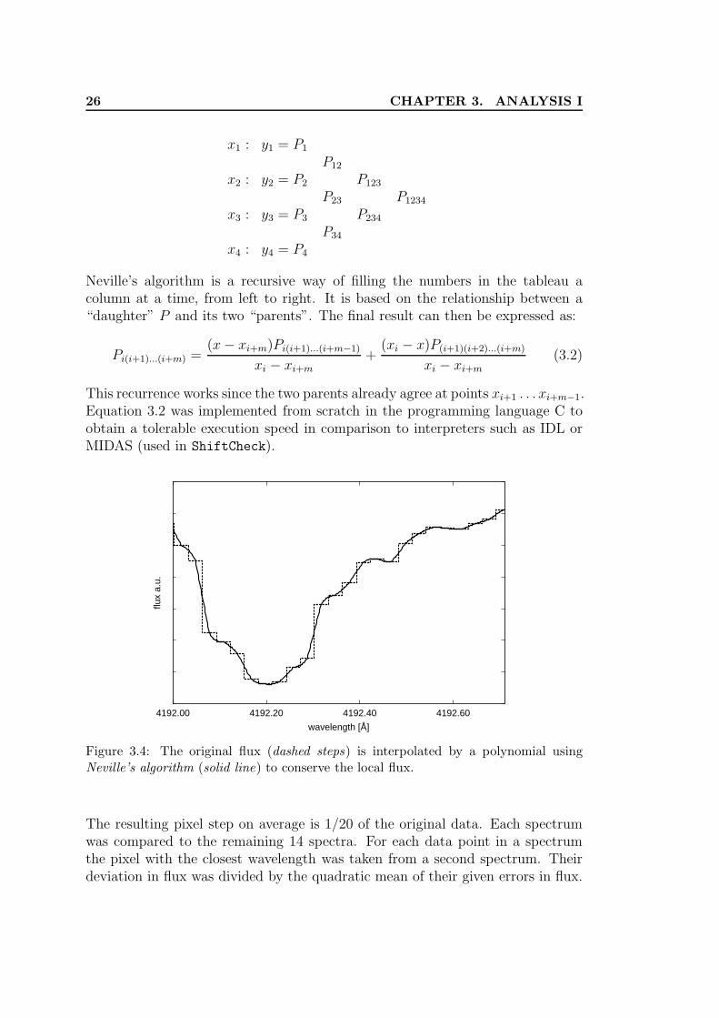
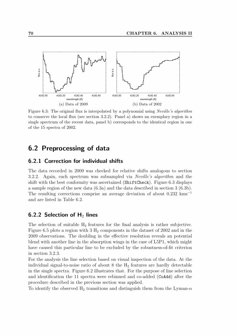
Figure 3.4: The original flux (dashed steps) is interpolated by a polynomial usingNeville’s algorithm (solid line) to conserve the local flux.

The resulting pixel step on average is 1/20 of the original data. Each spectrumwas compared to the remaining 14 spectra. For each data point in a spectrumthe pixel with the closest wavelength was taken from a second spectrum. Theirdeviation in flux was divided by the quadratic mean of their given errors in flux.


−30 −20 −10 0 10 20 30 40

χ2

shift between two separate spectra [mÅ]

fitted shift 6.2 mÅ

parabolic fit

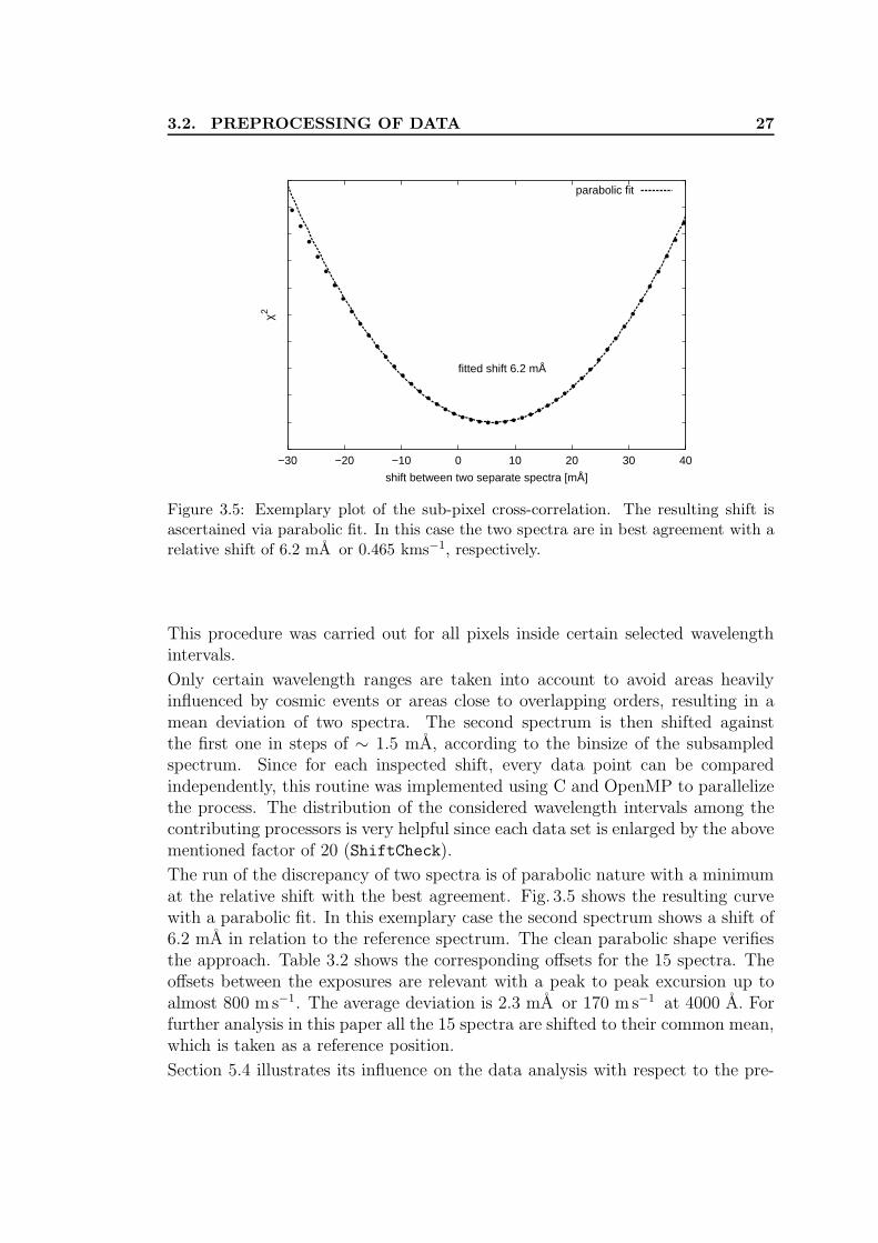
Figure 3.5: Exemplary plot of the sub-pixel cross-correlation. The resulting shift isascertained via parabolic fit. In this case the two spectra are in best agreement with arelative shift of 6.2 mA or 0.465 kms−1, respectively.

This procedure was carried out for all pixels inside certain selected wavelengthintervals.

Only certain wavelength ranges are taken into account to avoid areas heavilyinfluenced by cosmic events or areas close to overlapping orders, resulting in amean deviation of two spectra. The second spectrum is then shifted againstthe first one in steps of ∼ 1.5 mA, according to the binsize of the subsampledspectrum. Since for each inspected shift, every data point can be comparedindependently, this routine was implemented using C and OpenMP to parallelizethe process. The distribution of the considered wavelength intervals among thecontributing processors is very helpful since each data set is enlarged by the abovementioned factor of 20 (ShiftCheck).

The run of the discrepancy of two spectra is of parabolic nature with a minimumat the relative shift with the best agreement. Fig. 3.5 shows the resulting curvewith a parabolic fit. In this exemplary case the second spectrum shows a shift of6.2 mA in relation to the reference spectrum. The clean parabolic shape verifiesthe approach. Table 3.2 shows the corresponding offsets for the 15 spectra. Theoffsets between the exposures are relevant with a peak to peak excursion up toalmost 800 m s−1. The average deviation is 2.3 mA or 170 m s−1 at 4000 A. Forfurther analysis in this paper all the 15 spectra are shifted to their common mean,which is taken as a reference position.

Section 5.4 illustrates its influence on the data analysis with respect to the pre-


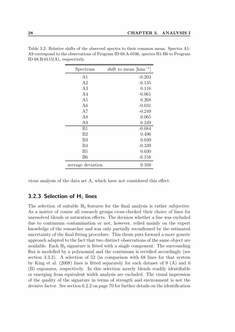
Table 3.2: Relative shifts of the observed spectra to their common mean. Spectra A1-A9 correspond to the observations of Program ID 68.A-0106, spectra B1-B6 to ProgramID 68.B-0115(A), respectively.

Spectrum shift to mean [kms−1]

A1 -0.203A2 -0.135A3 0.116A4 -0.061A5 0.268A6 -0.031A7 -0.249A8 0.065A9 0.249B1 -0.084B2 0.496B3 0.039B4 -0.339B5 0.030B6 -0.158

average deviation 0.168

vious analysis of the data set A, which have not considered this effect.

3.2.3 Selection of H2 lines

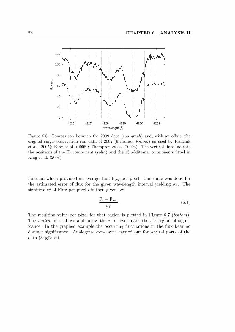
The selection of suitable H2 features for the final analysis is rather subjective.As a matter of course all research groups cross-checked their choice of lines forunresolved blends or saturation effects. The decision whether a line was excludeddue to continuum contamination or not, however, relied mainly on the expertknowledge of the researcher and was only partially reconfirmed by the estimateduncertainty of the final fitting procedure. This thesis puts forward a more genericapproach adapted to the fact that two distinct observations of the same object areavailable. Each H2 signature is fitted with a single component. The surroundingflux is modelled by a polynomial and the continuum is rectified accordingly (seesection 3.3.2). A selection of 52 (in comparison with 68 lines for that systemby King et al. (2008) lines is fitted separately for each dataset of 9 (A) and 6(B) exposures, respectively. In this selection merely blends readily identifiableor emerging from equivalent width analysis are excluded. The visual impressionof the quality of the signature in terms of strength and environment is not thedecisive factor. See section 6.2.2 on page 70 for further details on the identification


4226 4227 4228 4229 4230 4231

flux

a.u.


Figure 3.6: The 6 single spectra of set B (top), the 9 spectra of set A (below) separatedby the slashed line and (not to scale) the corresponding co-added data (bottom) areplotted around the region of L4R1 (vertical line).

of H2 signatures.Each rotational level is fitted with conjoined line parameters except for the red-shift naturally. The data are not co-added but analyzed simultaneously via thefitting procedure applied by Quast et al. (2005).

For each of the 52 lines there are two resulting fitted redshifts or observed wave-lengths, respectively, with their error estimates. To avoid false confidence, thesingle lines are not judged by their error estimate but by their difference in wave-length between the two data sets in relation to the combined error estimate. Theabsolute offset ∆λeffective to each other is expressed in relation to their combinederror given by the fit:

∆λσΣ1,2=

∆λeffective√

σ2λ1

+ σ2λ2

. (3.3)

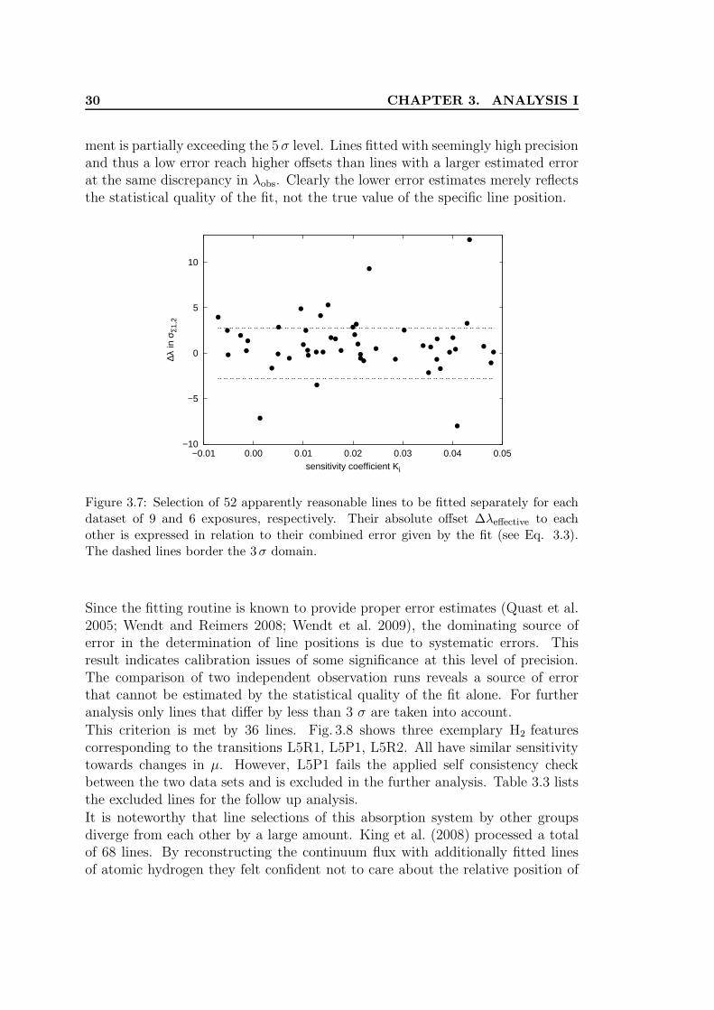
Figure 3.7 reveals notable discrepancies between the two datasets, the disagree-


ment is partially exceeding the 5σ level. Lines fitted with seemingly high precisionand thus a low error reach higher offsets than lines with a larger estimated errorat the same discrepancy in λobs. Clearly the lower error estimates merely reflectsthe statistical quality of the fit, not the true value of the specific line position.

−10

−5

0

5

10

−0.01 0.00 0.01 0.02 0.03 0.04 0.05

∆λ in

σΣ1

,2

sensitivity coefficient Ki

Figure 3.7: Selection of 52 apparently reasonable lines to be fitted separately for eachdataset of 9 and 6 exposures, respectively. Their absolute offset ∆λeffective to eachother is expressed in relation to their combined error given by the fit (see Eq. 3.3).The dashed lines border the 3σ domain.

Since the fitting routine is known to provide proper error estimates (Quast et al.2005; Wendt and Reimers 2008; Wendt et al. 2009), the dominating source oferror in the determination of line positions is due to systematic errors. Thisresult indicates calibration issues of some significance at this level of precision.The comparison of two independent observation runs reveals a source of errorthat cannot be estimated by the statistical quality of the fit alone. For furtheranalysis only lines that differ by less than 3 σ are taken into account.

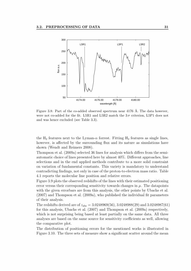
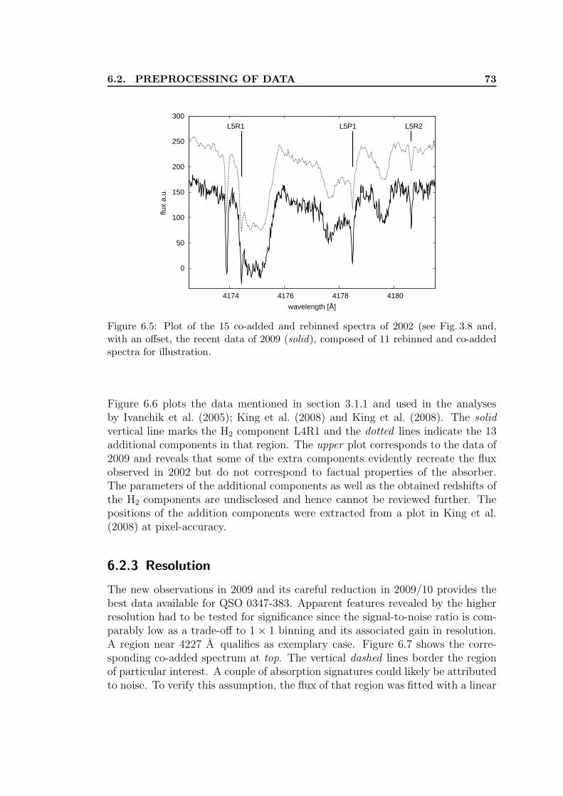
This criterion is met by 36 lines. Fig. 3.8 shows three exemplary H2 featurescorresponding to the transitions L5R1, L5P1, L5R2. All have similar sensitivitytowards changes in µ. However, L5P1 fails the applied self consistency checkbetween the two data sets and is excluded in the further analysis. Table 3.3 liststhe excluded lines for the follow up analysis.

It is noteworthy that line selections of this absorption system by other groupsdiverge from each other by a large amount. King et al. (2008) processed a totalof 68 lines. By reconstructing the continuum flux with additionally fitted linesof atomic hydrogen they felt confident not to care about the relative position of


50

100

150

200

250

300

4174.00 4176.00 4178.00 4180.00

flux

a.u.

wavelength [Å]

L5R1 L5P1 L5R2

Figure 3.8: Part of the co-added observed spectrum near 4176 A. The data however,were not co-added for the fit. L5R1 and L5R2 match the 3σ criterion, L5P1 does notand was hence excluded (see Table 3.3).

the H2 features next to the Lyman-α forrest. Fitting H2 features as single lines,however, is affected by the surrounding flux and its nature as simulations haveshown (Wendt and Reimers 2008).

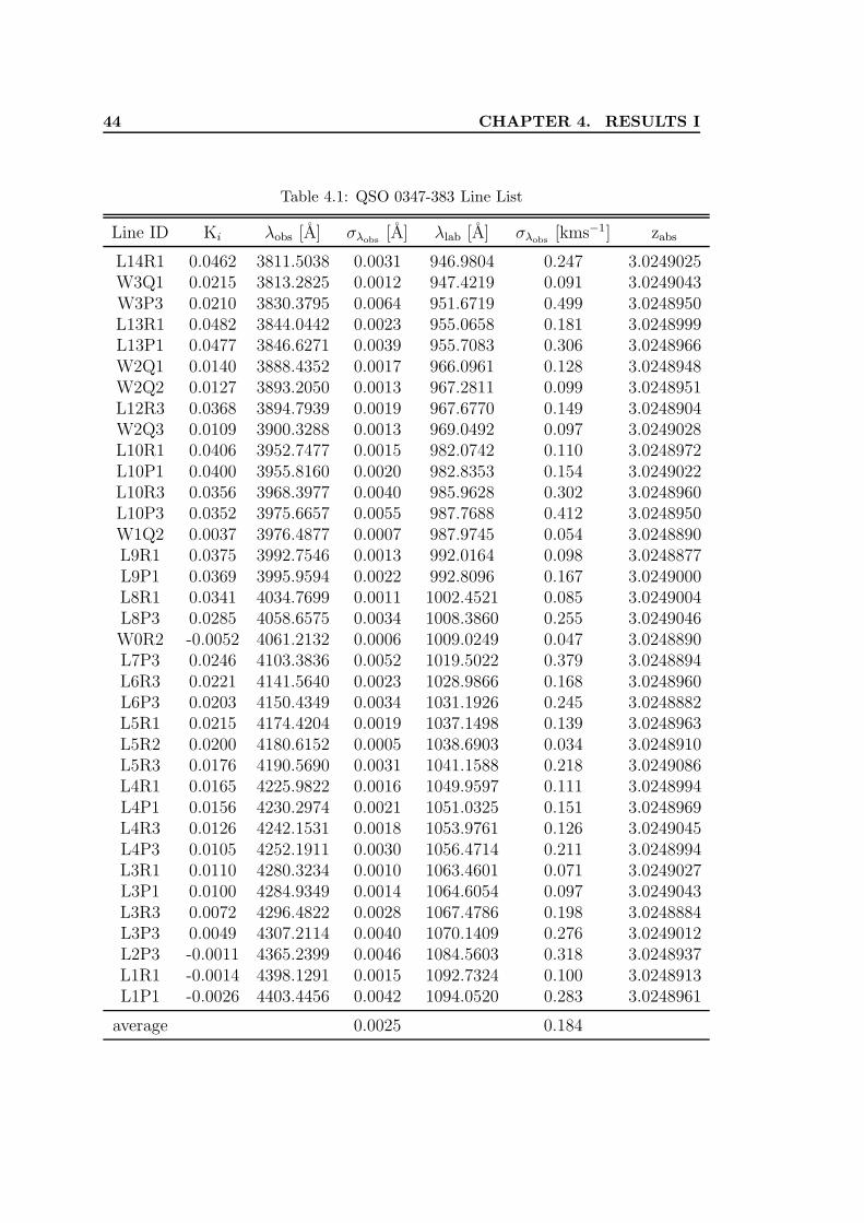
Thompson et al. (2009a) selected 36 lines for analysis which differs from the semi-automatic choice of lines presented here by almost 40%. Different approaches, lineselections and in the end applied methods contribute to a more solid constrainton variation of fundamental constants. This variety is mandatory to understandcontradicting findings, not only in case of the proton-to-electron mass ratio. Table4.1 reports the molecular line position and relative errors.

Figure 3.9 plots the observed redshifts of the lines with their estimated positioningerror versus their corresponding sensitivity towards changes in µ. The datapointswith the given errorbars are from this analysis, the other points by Ubachs et al.(2007) and Thompson et al. (2009a), who published the individual fit parametersof their analysis.

The redshifts derived are of zabs = 3.0248969(56), 3.0248988(29) and 3.0248987(61)for this analysis, Ubachs et al. (2007) and Thompson et al. (2009a) respectively,which is not surprising being based at least partially on the same data. All threeanalyses are based on the same source for sensitivity coefficients as well, allowingthe comparative plot.

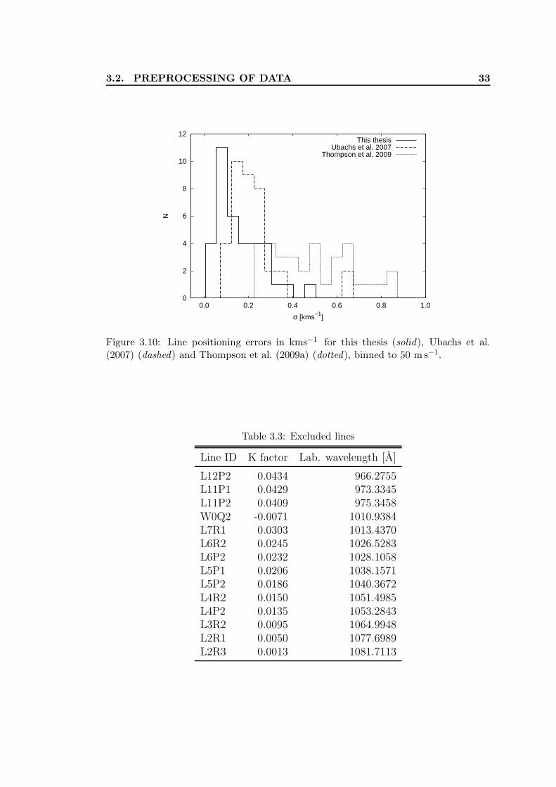
The distribution of positioning errors for the mentioned works is illustrated inFigure 3.10. The three sets of measure show a significant scatter around the mean


3.024880

3.024885

3.024890

3.024895

3.024900

3.024905

3.024910

3.024915

−0.01 0.00 0.01 0.02 0.03 0.04 0.05 0.06

reds

hift


This thesisUbachs 2007

Thompson 2009

Figure 3.9: Final results in redshift vs. sensitivity coefficient Ki for this analysis (cir-cles), Ubachs et al. (2007) (squares) and Thompson et al. (2009a) (triangles).

quite in excess of the error in line position which is suggestive of the presence ofsystematic errors.The chosen ∆λ criterion for line selection permits evaluation of the self-consistencyof a line positioning via fit for the involved data. While the availability of twoindependent observations on short time scale is rather special, it illustrates oneapplicable modality to avoid relying on the fitting apparatus alone.


0

2

4

6

8

10

12

0.0 0.2 0.4 0.6 0.8 1.0

N

σ [kms−1]

This thesisUbachs et al. 2007

Thompson et al. 2009

Figure 3.10: Line positioning errors in kms−1 for this thesis (solid), Ubachs et al.(2007) (dashed) and Thompson et al. (2009a) (dotted), binned to 50 m s−1.

Table 3.3: Excluded lines

Line ID K factor Lab. wavelength [A]

L12P2 0.0434 966.2755L11P1 0.0429 973.3345L11P2 0.0409 975.3458W0Q2 -0.0071 1010.9384L7R1 0.0303 1013.4370L6R2 0.0245 1026.5283L6P2 0.0232 1028.1058L5P1 0.0206 1038.1571L5P2 0.0186 1040.3672L4R2 0.0150 1051.4985L4P2 0.0135 1053.2843L3R2 0.0095 1064.9948L2R1 0.0050 1077.6989L2R3 0.0013 1081.7113


3.3 Fitting

Since the methods for fitting a theoretical line profile to observed data is manifoldsome possible procedures are described in more detail. As a first step an initialset of parameters is evaluated. Most fitting procedures depend on a reasonablemanually selected set to bring the iterative algorithm on the right track so tospeak. The most naive approach is to fit a line feature by a model based on theinitial set and then vary each free parameter independently to find a minimumin the objective function describing the discrepancy between observation and fit.

This approach is of course unpractical, since the number of necessary calculationsof the synthetic profile increases exponentially with each free parameter. Also theparameter range and resolution must be set sufficiently large to ensure a globalminimum. Furthermore a reasonable range must be manually selected to assurethat the covered parameter space does include the best-fit parameters.

Only very recently some groups experiment with exploration of the whole param-eter space. King et al. (2008) for example implemented a Monte Carlo methodto cover all possible combinations of fitting parameters. Unfortunately MonteCarlo methos scale exponentially with increasing dimensionality and are henceimpractical for non-trivial situations. A slight improvement was achieved bythe utilization of Markov Chain Monte Carlo simulations. The combination ofMarkov Chain methods and Monte Carlo simulation degrades merely polynomialwith higher dimensionality but also introduces non-trivial correlation betweensamples and can in principle not be parallelized. Furthermore the underlyingprobability distribution has to be preassigned. It is therefor not feasible for real-istic fitting tasks with todays computer power.

Even though it proves to be an valuable technique to estimate the statisticalprecision of a certain set of parameters, it cannot reveal anything about theaccuracy of the data modelling and further does not produce traceable results. Itshould only be used as an supplemental method.

To avoid the need to inspect the whole parameter space, the common approachis to collect information about the local topology of the objective function bycalculating its partial derivatives for each free parameter. This ensures a farmore rapid convergence to a nearby minimum. This method (as implemented inthe Levenberg-Marquardt algorithm for example) has the deficiency of relying onthe initial parameter set, since in a straight forward implementation of this algo-rithm, possibly only a local minimum is found – depending on the situation notnecessarily the global minimum. The first iteration step is based on the initiallyselected parameter set. Afterwards a second set of parameters is evaluated. TheLevenberg-Marquardt algorithm interpolates a gradient of χ2 in respect to thefree model parameters and thereby ascertains the “direction” in the parameterspace towards the local minimum. The second derivative of χ2, more generally

3.3. FITTING 35

the Hessian matrix4 delivers the appropriate stepsize for each parameter. De-pending on the implementation, this stepsize is scaled additionally to match therequired needs. A new parameter set based on the information of the directionand the selected stepsize is evaluated and in case of a smaller χ2 value used asfulcrum for the next iterationstep. The additional scaling is used to increasethe resolution in the parameterspace with each iteration step. The iteration iscompleted when the change between successive χ2 values falls below a certainthreshold value. The value of the minimal χ2 depends on the number of effectivedegrees of freedom. A value independent on the number of data points or theselected model is described by the normalized χ2:

χ2norm =

χ2

r. (3.4)

In the ideal case the final value of χ2norm reaches unity. That would mean that

the total deviation between model and data equals the measurement errors of thedata. A value below 1 thus indicates an invalid model or overestimated individualerrors σi.The approach applying evolutionary algorithms, such as the code implementedby Quast et al. (2005) that is used here, is based on stochastics (see, e.g., Hansenand Ostermeier 2001). The principle is similar to the one described above butinstead of a manual first guess of initial parameters, several sets of random initialparameters are computed automatically over a parameter range that merely needsrough preselection. The most successful of those build the centres of other groupsof random, yet less wide spread sets of parameters and so forth. This stochas-tic approach can additionally be fine- tuned by adjusting the expansiveness ofeach successive group of random parameters in both the parameter space and inquantity. With a sufficiently widespread cluster of parameter sets, theoreticallythe global minimum will always be reached. In practice a compromise must befound between computing time and success in reaching the global minimum. Itsdrawback is of course its inefficiency in terms of computing power and the need tocheck up the final fit on physically reasonable parameters. However, the principleof evaluating multiple groups of parametersets independently of each other allowsfor consequent parallel computing.The element of randomness requires a full completion of the iterative process.Whilst the Levenberg-Marquardt algorithm usually converges rather soon towardsthe final parameters the evolutionary procedure can only give reliable resultsafter all branches of parameter groups are evaluated. Some principle problemsof redundancy in parameter sets for complex models have yet to be overcome aswell. In praxis two or multiple line profiles whose parameter spaces significantlyoverlap can cause the algorithm to lock up on rare occasions. The dynamical

4The Hessian matrix is the square matrix of second partial derivatives of a scalar-valuedfunction.


scaling towards regions with small Hessian matrix to gain higher resolution isimplemented by an increasingly smaller scattering of random parameter sets forsuccessive child populations of parameter sets.

This fitting program uses a simplified pseudo-Voigt-function to generate the syn-thetic line profiles. For weak lines a mere gaussian profile would suffice sincenatural line broadening has no noticeable impact on the line shapes.

The program of Quast et al. (2005) was written in C++ under the applicationof OpenMP to parallelize the fitting procedure and distribute the computationof the individual parameter sets among the available CPU cores. The problemscales very well and the accumulated time for a complete fit in a multitude ofspectra is justifiable.

Merely with minor adjustments mainly in the input/output interface, the fittingprocedure could be adjusted to the special requirements when probing a variationin µ (RQFit).

The limitation of OpenMP, one single shared memory for all processes workingin parallel plays no major role since the computations though large in numberare comparably simple in detail and do not require notably large amounts ofmemory.

3.3.1 Simultaneous fit vs. co-added fit

The fitting program as described in the preceding section has the ability to fitseveral lines simultaneously to one subset of free parameters. Individual parame-ters can be cross referenced to each other and the code is under the constraint tofind one best joint fit for these parameters. This feature is of great conveniencesince several line parameters as broadening width or column density are usuallyshared by a whole group of lines and do not differ among each other. This concepthas even been expanded to fit several separate spectra simultaneously. So evenfor overlapping wavelength regions, the continuum and for example the redshiftare fitted locally but the line width is fitted to all participant spectra and lines.

This method appears to be superior to a rough prior co-adding of spectra. Manyerrors coarse co-addition might introduce can be avoided by this way, since thereis no need to rebin the data. Usually, rebinning leads to even-spaced data pointsand the flux is redistributed among the single bins. This degrades the originalalignment of the reduced data, which – for geometric reasons concerning theprojection onto the CCD chip and later reductions steps like the vacuum-aircorrection – has a differential gradient of spacing. See, e.g., Levshakov et al.(2002) for a discussion of this effect.

A rebin would introduce a stronger correlation of pixels. The impact of suchcorrelations on the results is not well-known (see, e.g., Aitken 1934). A χ2 min-imization procedure does rely on independent data points though. The conceptof simultaneous fit has the advantage of taking physical conditions into account

3.3. FITTING 37

in form of further restrictions on the degrees of freedom.

3.3.2 Continuum handling

An accurate estimate of the true continuum of a spectrum is essential for a goodfit of an absorption line. Especially for optically thin lines the determined col-umn density is very sensitive to variations in the continuum fit. Particularly indamped Lyman-α systems (DLA) at large redshifts there hardly is any unblendedcontinuum detectable in the range of H2 absorption due to the Lyman-α forrest.There are numerous techniques and strategies to gain a reliable estimation of thetrue continuum despite its contamination.

A rather generic approach is specific to pure absorption spectra and assumingthat the data points with the highest photon count contribute to the continuum,since there are no emission features. Therefore a polynomial function of low orderis fitted iteratively to a selected subset of data points above a certain threshold.This threshold is increased or rather the range between Fluxmin and Fluxmax (ifthere are some spikes or cosmics in the spectra) is narrowed with each iterationstep until a minimum variance or the predefined minimum number of selecteddata points is reached. This method is only applicable though when a reasonableamount of undisturbed continuum emission is present in the wavelength range ofinterest and hence not applicable to the spectra at hand.

Another way of dealing with the continuum is to construct it manually. The curveof the estimated continuum is drawn or based on some interpolation points. Thecontinuum level simply is set at the upper end of an absorption line feature todisregard all influences of other lines nearby. Dealing with the continuum inthis manner yields a great uncertainty that only a curve of growth analysis canreveal. Albeit this is one of the few options to deal with heavily contaminatedand partially blended lines at all and was carried out by Ivanchik et al. (2002)for example.

A refinement of the latter approach is to not only fit the one line of interestand border it by an artificial continuum but to fit a series of lines with freeparameters to match the disturbed measured flux. The actual line of interestis then embedded into a group of lines that are used to fit the surrounding fluxlevel. The true continuum, however, needs to be estimated but for a larger lessalternating environment. In some cases the extra lines may disturb the shape ofthe measured main component and this procedure needs special supervision.

In this work, the continuum is fitted by the code together with the lines. The fitis based on the flux adjoining the line feature. The accuracy of the continuumfit increases significantly by the option of simultaneous fitting. All molecularhydrogen lines observed at the same rotational level should have identical physicalproperties, as in column density and line width. This constrains the uncertaintyof the continuum since the resulting column density has to be consistent with


the simultaneous fits of the more secure continuum regions and the identifiedH2 absorption features are spread over the full range of the observed spectrum.However, a mere χ2 consideration to evaluate the quality of the fit is invalid, sincethe model of a single line does not describe the observed flux sufficiently.In cases of a continuum flux with apparent influences of broad Lyman-α featuresor general contamination, a parabolic or cubic function was used to fit the back-ground to the observed flux. See Figure 3.11 of L3R3 and L6R3 for an exemplarof a parabolic fit. These exemplary lines already represent the extreme end ofnon-constant bordering continuum flux.

0

1

2

3

4

−50 0 50

flux

a.u.

radial velocity [kms−1]

(a) L3R3

0

1

2

3

−50 0 50

flux

a.u.

radial velocity [kms−1]

(b) L6R3

Figure 3.11: Exemplary cases of continuum matching via parabolic fit to the observedflux for the Lyman lines L3R3 and L6R3.

An additional issue not yet discussed in connection with varying µ are the oscilla-tor strengths. Whereas the transition frequencies have been revised several timesover the last few years with improved instrumentation and numerical methods(see section 2.2.3), the latest data for the oscillator strength of molecular hydro-gen are still from tables by Abgrall et al. (1993a,b). UV-laser experiments are notyet capable of arranging the required measurements: “The oscillator strengthscan only be derived by calculations based on coarse approximations. Verificationof the listed values of the oscillator strengths by experimental methods appearsimpossible at laboratory conditions at the present state.” (Ubachs, private com-munication).Uncertainties in the oscillator strengths are not directly reflected in the mea-sured line positions and hence the obtained redshift but they have influence onthe quality of fit and the determination of the continuum. In particular the ap-proach to fit a designated number of arbitrary line components in the vicinity of

3.3. FITTING 39

H2 profiles is in particular error-prone to wrong oscillator strengths and thereforewrong equivalent widths.Groups that apply this multi-component fit (see, e.g., King et al. 2008), in generaladd further components to a fit-region around a H2 signature, until the lowestχ2 value is reached. Alternatively, the residuals are inspected for remaining fluxbeyond the noise level.This approach is vulnerable to wrong oscillator strengths and in the same way tounderestimated errors of the observed flux (see section 3.2.1 for more details).

4 Results I

4.1 Determination of ∆µ/µ

For the final analysis the selected 36 lines are fitted in all 15 shifted, error-scaledspectra simultaneously (see section 3.2.3 for details on the line selection criteria).The result of an unweighted linear fit corresponds to

∆µ/µ = (15 ± 16) × 10−6, (4.1)

at zabs = 3.025. The stated finding of Eq. 4.1 can be translated into a rateof change. When imposing the assumptions of a linear cosmological expansionmodel, the redshift z is related to the look-back time T via:

T = T0

[

1 − (1 + z)−3/2]

, (4.2)

with T0 the age of the universe, which may be set at 13.7 Gyrs. For the quasarunder consideration this yields a look-back time of ∼ 12 Gyrs. With the furtherassumption that µ has varied linearly over time this corresponds to a rate ofchange of dlnµ/dt = −1.2 × 1015 yr−1. The negative sign must be interpreted asa decrease in µ over time.This conversion into a rate is merely exemplary, however. The findings of thisanalysis yield no indication of variation with the current limit of accuracy.Figure 4.1 shows the resulting plot. The complete list of lines is shown in Table4.1.The approach to apply an unweighted fit is a consequence of the unknown natureof the prominent systematics. Uncertainties in wavelength calibration cannot beexpressed directly as an individual error per line. The graphed scatter in redshiftcan not be explained by the given positioning errors alone. The likeliness of thedata with the attributed error being linearly correlated is practically zero. Thefit to the data is not self-consistent. For this work the calibration errors andthe influence of unresolved blends are assumed to be dominant in comparison toindividual fitting uncertainties per feature.For the following analysis the same error is adopted for each line. With anuncertainty in redshift of 1× 10−6 we obtain: ∆µ/µ = (15± 6)× 10−6. Howeverthe goodness-of-fit is below 1 ppm and is not self consistent. Judging by that andFig. 4.1, a reasonable error in observed redshift should at least be in the order of4 × 10−6. The weighted fit gives: ∆µ/µ = (15 ± 14) × 10−6.

4.1. DETERMINATION OF ∆µ/µ 41

−15.00

−10.00

−5.00

0.00

5.00

10.00

15.00

20.00

−0.01 0.00 0.01 0.02 0.03 0.04 0.05

redu

ced

reds

hift

×10

6


J=1J=2J=3

Figure 4.1: The unweighted fit to the measured redshifts of the H2 components in QSO0347-383 corresponds to ∆µ/µ = (15 ± 16) × 10−6. The error bars represent merely tothe fitting uncertainty in the order of 180 m s−1 on average. Note, that at such a highscatter zKi=0 differs from z by less than 1 σz.

This approach is motivated by the goodness-of-fit test:Q(χ2|ν) is the probability that the observed chi-square will exceed the value χ2

by chance even for a correct model, ν is the number of degrees of freedom. Givenin relation to the incomplete gamma function:

Q(χ2|ν) = Γ

(

ν

2,χ2

2

)

. (4.3)

Assuming a gaussian error distribution, Q gives a quantitative measure or thegoodness-of-fit of the model. If Q ist very small for some particular data set, thenthe apparent discrepancies are unlikely to be chance fluctuations. More probableis either that the model is wrong or the size of the measurement errors is largerthan stated. However, the chi-square probability Q does not directly measurethe credibility of the assumption that the measurement errors are normally dis-tributed. In general, models with Q < 0.001 can be considered unacceptable. Inthis case the model is given and hence the low probability is due to underesti-mated errors in the data. Solely for given errors of ∼ 300 m s−1, corresponding to∼ 4×10−6 in redshift for QSO 0347-383 the goodness-of-fit parameter Q exceeds0.001. The scale of the error appears to be ∼ 300 m s−1 to achieve a self-consistentfit to the data.For the data on QSO 0347-383 this corresponds to an error in the observedwavelength of roughly 4 mA, which is notably larger than the estimated errors

42 CHAPTER 4. RESULTS I

for the individual line fits which ranges from 0.5 mA to 6.5 mA with an average of2.5 mA (∼ 180 m s−1). The systematic error contributes an uncertainty of about2 mA on average. The immediate calibration errors are in the order of 50 m s−1forset B and presumably slightly larger for set A (see section 3.1.1). Figure 4.2 plotsthe data with errorbars corresponding to 180 m s−1 and the total of 300 m s−1.

−15

−10

−5

0

5

10

15

20

−0.01 0.00 0.01 0.02 0.03 0.04 0.05

redu

ced

reds

hift

×10

6


J=1J=2J=3

Figure 4.2: The data points are identical to Fig. 4.1. Here, the error bars representthe average positioning error (solid) and the additional systematic error (dotted) of∼ 180 m s−1 and ∼ 120 m s−1, respectively.

The final result can be subdivided as:

∆µ/µ =(

15 ± (9stat + 6sys))

× 10−6. (4.4)

The comparably high scatter in Figure 4.1 can partially be attributed to the ap-proach to fit single H2 components with a polynomial fit to the continuum. In spe-cial cases, contaminated flux bordering a H2 signature can introduce additionaluncertainty in positioning. Therefore checks for self-consistency and systematicsare of utmost importance.

The determination of the different errors involved is on a par with the actualresult. We believe that this result represents the limit of accuracy that canbe reached with the given data set and the applied methods for analysis. Thepresented method yields a null result. The recent work by Thompson et al.(2009a) stated ∆µ/µ = (−28 ± 16) × 10−6 for a weighted fit based on the samesystem in QSO 0347-383. The stated errors in that work reflect the statisticaluncertainties alone.


Note, that the given systematics of 2.7ppm for Keck/HIRES data given in Malecet al. (2010) are in first approximation estimated by the observed ∼500m s−1

peak-to-peak intra-order value reduced according to the number of moleculartransitions observed, e.g. ∼ 500 m s−1/

√93 ∼ 52 m s−1.

The approach in Malec et al. (2010) neglects the very nature of systematic errorsas they present an absolute limit to the achievable accuracy and thus – in contrastto statistical errors – cannot be reduced by larger samples (see also section 5.2).


Table 4.1: QSO 0347-383 Line List

Line ID Ki λobs [A] σλobs[A] λlab [A] σλobs

[kms−1] zabs

L14R1 0.0462 3811.5038 0.0031 946.9804 0.247 3.0249025W3Q1 0.0215 3813.2825 0.0012 947.4219 0.091 3.0249043W3P3 0.0210 3830.3795 0.0064 951.6719 0.499 3.0248950L13R1 0.0482 3844.0442 0.0023 955.0658 0.181 3.0248999L13P1 0.0477 3846.6271 0.0039 955.7083 0.306 3.0248966W2Q1 0.0140 3888.4352 0.0017 966.0961 0.128 3.0248948W2Q2 0.0127 3893.2050 0.0013 967.2811 0.099 3.0248951L12R3 0.0368 3894.7939 0.0019 967.6770 0.149 3.0248904W2Q3 0.0109 3900.3288 0.0013 969.0492 0.097 3.0249028L10R1 0.0406 3952.7477 0.0015 982.0742 0.110 3.0248972L10P1 0.0400 3955.8160 0.0020 982.8353 0.154 3.0249022L10R3 0.0356 3968.3977 0.0040 985.9628 0.302 3.0248960L10P3 0.0352 3975.6657 0.0055 987.7688 0.412 3.0248950W1Q2 0.0037 3976.4877 0.0007 987.9745 0.054 3.0248890L9R1 0.0375 3992.7546 0.0013 992.0164 0.098 3.0248877L9P1 0.0369 3995.9594 0.0022 992.8096 0.167 3.0249000L8R1 0.0341 4034.7699 0.0011 1002.4521 0.085 3.0249004L8P3 0.0285 4058.6575 0.0034 1008.3860 0.255 3.0249046W0R2 -0.0052 4061.2132 0.0006 1009.0249 0.047 3.0248890L7P3 0.0246 4103.3836 0.0052 1019.5022 0.379 3.0248894L6R3 0.0221 4141.5640 0.0023 1028.9866 0.168 3.0248960L6P3 0.0203 4150.4349 0.0034 1031.1926 0.245 3.0248882L5R1 0.0215 4174.4204 0.0019 1037.1498 0.139 3.0248963L5R2 0.0200 4180.6152 0.0005 1038.6903 0.034 3.0248910L5R3 0.0176 4190.5690 0.0031 1041.1588 0.218 3.0249086L4R1 0.0165 4225.9822 0.0016 1049.9597 0.111 3.0248994L4P1 0.0156 4230.2974 0.0021 1051.0325 0.151 3.0248969L4R3 0.0126 4242.1531 0.0018 1053.9761 0.126 3.0249045L4P3 0.0105 4252.1911 0.0030 1056.4714 0.211 3.0248994L3R1 0.0110 4280.3234 0.0010 1063.4601 0.071 3.0249027L3P1 0.0100 4284.9349 0.0014 1064.6054 0.097 3.0249043L3R3 0.0072 4296.4822 0.0028 1067.4786 0.198 3.0248884L3P3 0.0049 4307.2114 0.0040 1070.1409 0.276 3.0249012L2P3 -0.0011 4365.2399 0.0046 1084.5603 0.318 3.0248937L1R1 -0.0014 4398.1291 0.0015 1092.7324 0.100 3.0248913L1P1 -0.0026 4403.4456 0.0042 1094.0520 0.283 3.0248961

average 0.0025 0.184

4.2. RESULT VIA DISCRETE LINE PAIRS 45

4.2 Result via discrete line pairs

To accomplish a robust bound on the variation of µ, additional alternative ap-proaches are advisable. ∆µ/µ can also be obtained by using merely two lines thatshow different sensitivity towards changes in the proton-to-electron mass ratio.

The set of derived redshifts with their corresponding sensitivity coefficients issorted and pairs of two lines are selected via complete permutation. Line pairsthat differ in sensitivity below a certain threshold were rejected (ToPair).

Another criterion is their separation in the wavelength frame to avoid pairs of linesfrom different ends of the spectrum and hence in particular error-prone (see, e.g.,Griest et al. 2010). Several tests showed that a separation of ∆λ ≤ 110 A and arange of sensitivity coefficients K1-K2 ≥ 0.02 produces stable results that do notchange any further with more stringent criteria. Pairs that cross two neighboringorders (∼ 50 A) show no striking deviations either, which would have indicateddistinct problems in the wavelength calibration.

−200

−100

0

100

200

0.020 0.025 0.030 0.035 0.040 0.045 0.050 0.055

∆µ×

106 d

eriv

ed fr

om li

ne p

airs

Ki spread of line pair

Figure 4.3: ∆µ/µ derived from individual line pairs (52) which are separated by lessthan 110 A and show a difference in sensitivity of more then 0.02. The errorbarsreflect the combined positioning error of the two contributing lines. The weighted fitcorresponds to ∆µ/µ = (6 ± 12) × 10−6.The filled squares graph 11 line pairs, selected to give the largest difference in sensitivity(≥ 0.02) towards variation in µ (See Table 4.2).

Figure 4.3 graphs the different values for ∆µ/µ derived from 52 line pairs thatmatch the aforementioned criteria. Note, that a single observed line contributesto multiple pairs. Fitting of n line pairs that are sensitive to µ should be more


precise than that based on a single pair. However, the improvement is not as highas 1/

√n because the different pairs are partially correlated via the redshift (and

the sensitivity) of the same line that contributes to several pairs. If we considern redshift differences z1 − z0, z2 − z0, . . ., zn − z0, where z0 is the referenceredshift, then it is easy to show that the correlation coefficient κi,j between twoof them (i 6= j) is given by

κi,j =1

√

(1 + s2i )(1 + s2

j), (4.5)

where si = σzi/σz0

and si = σzj/σz0

. Taking into account that the computationalerrors in determined redshifts, σzi

, are almost equal, we have κi,j = κ ≈ 1/2.The covariance matrix Cov(zi − z0, zj − z0) contains n diagonal terms σ2 andn(n − 1) non-diagonal terms κσ2, where σ2 represents the variance in a singlemeasurement. The error in the mean redshift caused by the positioning uncer-tainties (referred to as εsys hereafter) can be calculated as described by, e.g.,Stuart and Ord (1994):

εsys =

[

n∑

i=1

n∑

j=1

ωiωjCov(zi − z0, zj − z0)

]1/2

. (4.6)

In cases of equal accuracy, the weight ωi = 1/n for each i. Then εsys is approxi-mately equal to

εsys =σ

n

√

n + n(n − 1)κ ≈ σ√

κ . (4.7)

Thus, the gain factor,√

κ, is only about 0.7 for the line pairs in question. Thisalternative approach is in general not suited to provide a more precise result butit can verify the findings through an independent method. The discussed limitin precision through large number statistics applies for all kind of samples thathold some correlation.The average value of the 52 redshifts-sensitivity ratios yields ∆µ/µ = 6±12×10−6.The scatter is then related to uncertainties in the wavelength determination whichis mostly due to calibration errors. The standard error is 8 × 10−6.The approach to use each observed line only once and thus avoid the mentionedcorrelation in the analysis is plotted in Fig. 4.3 as filled squares. The pairs toderive ∆µ/µ from were constructed by grouping the line with the highest sensi-tivity value together with the line corresponding to the lowest value for Ki and soon with the remaining lines. The distance in wavelength space between the twolines was no criterion and it ranges from 20A to 590A (see Table 4.2). Withoutreutilization of lines, 11 pairs with a coverage in sensitivity of ∆Ki ≥ 0.02 werefound.Evidently the usage of lines with comparably large distances in the spectrumhas no influence on the results. This indicates that the contribution of global


differential errors in the wavelength calibration appear to be small. Potentialsources of such deviations would be the vacuum-air correction for example.

Table 4.2: Grouping all observed lines into 17 pairs of maximum Ki sensitivity notconsidering their separation in wavelength space (rightmost column).

Line 1 Line 2 ∆µ/µ ∆Ki ∆λ [A]

W0R2 L13R1 50.5 ×10−6 0.0535 -217.2L1P1 L13P1 2.7 ×10−6 0.0503 -556.8L1R1 L14R1 58.6 ×10−6 0.0477 -586.6L2P3 L10R1 20.9 ×10−6 0.0417 -412.5W1Q2 L10P1 90.4 ×10−6 0.0364 -20.7L3P3 L9R1 -103.0 ×10−6 0.0326 -314.5L3R3 L9P1 97.6 ×10−6 0.0297 -300.5L3P1 L12R3 -128.9 ×10−6 0.0268 -390.1L4P3 L10R3 -33.9 ×10−6 0.0251 -283.8W2Q3 L10P3 -79.4 ×10−6 0.0243 75.3L3R1 L8R1 -24.0 ×10−6 0.0231 -245.6

L4R3 L8P3 3.1 ×10−6 0.0159 -183.5W2Q2 L7P3 -120.0 ×10−6 0.0119 210.2W2Q1 L6R3 34.0 ×10−6 0.0082 253.1L4P1 W3Q1 312.7 ×10−6 0.0059 -417.0L4R1 L5R1 -154.6 ×10−6 0.0050 -51.6L5R3 W3P3 -996.4 ×10−6 0.0034 -360.2

5 Error Analysis I

5.1 Quality of fit

A least-squares fit to the unweighted redshift versus sensitivity coefficient datacan only yield the best fit to the data. It is not trivial to ascertain the quality ofthe fit (see chapter 4.1).The uncertainties of the fit merely represent the certainty to which the foundparameters describe indeed the best possible fit. It is not directly correlated tothe distribution of the data itself and of course, it contains no information at allon the systematics underlying the data.The weighted fit in principle is more suited to represent the quality of the dataand its distribution but it is strongly biased by the uncertainty of the contributingerrors. This is obvious for the present data with estimated positioning errors perline, that fail to reflect the scatter of the data.A diverse approach to examine data is via the bootstrap method (see, e.g., Efronand Tibshirani 1986).Bootstrapping is the practice of estimating properties of an estimator (such as itsvariance) by measuring those properties when sampling from an approximatingdistribution. One standard choice for an approximating distribution is the empir-ical distribution of the observed data. In the case where a set of observations canbe assumed to be from an independent and identically distributed population,this can be implemented by constructing a number of resamples of the observeddataset (and of equal size to the observed dataset), each of which is obtained byrandom sampling with replacement from the original dataset.For the data at hand this implies to select samples of 36 lines of the data setof observed lines. The linear fit to the measured redshift against the sensitivitydata is applied to this new sample. This is redone for a large number of randomlyselected samples. For 36 lines there are evidently 3636 possible samples, includingall permutations of the same lines though. A few thousand samples are sufficientin general and Figure 5.1 shows the histogram of ∆µ/µ derived from 10.000bootstrap samples.Again the algorithm to perform the resampling and this large amount of least-square fits is implemented in C and OpenMP, since the individual fits are inde-pendent of each other and can easily be parallelized (BootStrap). The histogramis generated with a binning of 1 × 10−6 and Figure 5.1 also contains the fit ofa gaussian (solid line) to the data. The distribution of the ∆µ/µ is slightly

5.1. QUALITY OF FIT 49

asymmetric but this has no impact on the findings.The result of the bootstrap analysis corresponds to:

∆µ/µ = (14.9 ± 12.0) × 10−6. (5.1)

This verifies the results and in particular the error estimation of section 4.1 thatyielded ∆µ/µ =

(

15 ± (9stat + 6sys))

× 10−6.The FWHM of the bootstrap analysis incorporate the scatter of the data auto-matically and is in good agreement with the estimation of the systematic errorsvia goodness of fit tests. The FWHM of the Gaussian profile is:

FWHM = 2σ√

2ln(2). (5.2)

The uncertainty corresponds to the inflection points of the gaussian curve andcan be derived from the width of a fitted gaussian via σ ∼ FWHM/2.35.

0

0.2

0.4

0.6

0.8

1

−40 −20 0 20 40 60

∆µ/µ×106

Figure 5.1: ∆µ/µ and in particular its uncertainty derived via 10.000 bootstrap samples.The gaussian fit yields a centroid at 14.9 and a FWHM of 28.2.

50 CHAPTER 5. ERROR ANALYSIS I

5.2 Standard Error

The terms “standard error” and “standard deviation” are often confused. Thecontrast between these two terms reflects the important distinction between datadescription and inference.The standard deviation is a measure of variability. When we calculate the stan-dard deviation of a sample, we are using it as an estimate of the variability ofthe population from which the sample was drawn. For data with a normal dis-tribution, about 95% of individuals will have values within 2 standard deviationsof the mean, the other 5% being equally scattered above and below these limits.Contrary to popular misconception, the standard deviation is a valid measure ofvariability regardless of the distribution. About 95% of observations of any dis-tribution usually fall within the 2 standard deviation limits, though those outsidemay all be at one end.When we calculate the sample mean we are usually interested not in the mean ofthis particular sample, but in the mean for individuals of this type-in statisticalterms, of the population from which the sample comes. We usually collect datain order to generalize from them and so use the sample mean as an estimate ofthe mean for the whole population. Now the sample mean will vary from sampleto sample; the way this variation occurs is described by the “sampling distribu-tion” of the mean. We can estimate how much sample means will vary from thestandard deviation of this sampling distribution, which we call the standard error(SE) of the estimate of the mean. As the standard error is a type of standarddeviation, confusion is understandable. Another way of considering the standarderror is as a measure of the precision of the sample mean.The standard error of the sample mean depends on both the standard deviationand the sample size, by the simple relation SE = SD/

√samplesize. The standard

error falls as the sample size increases, as the extent of chance variation is reduced.By contrast the standard deviation will not tend to change with the size of oursample.If we want to state how widely scattered some measurements are, we use thestandard deviation. If we want to indicate the uncertainty around the estimateof the mean measurement, we quote the standard error of the mean.Hence, the standard error is not suited to describe the quality of a data set, itmerely represents the precision of a particular fit for example, not its accuracy.

5.3. UNCERTAINTIES IN THE SENSITIVITY COEFFICIENTS 51

5.3 Uncertainties in the sensitivity coefficients

At the current level of precision, the influence of uncertainties in the sensitiv-ity coefficients Ki is minimal. It will be of increasing importance though whenwavelength calibration can be improved by pedantic demands on future obser-vations. Eventually Laser Frequency Comb calibration will allow for practicallyarbitrary precision and uncertainties in the calculations of sensitivities will playa role. The wavelength data for molecular hydrogen available is adequate evenfor the next generation telescopes, like the European Extremely Large Telescope(ELT) currently planned for 2018 (see, e.g., Molaro 2009). Higher resolution inthe data will hence directly influence the positioning errors (see Chapter AnalysisII). Commonly, the weighted fits neglects the error in Ki completely, which maybecome inappropriate in the near future.Effective analysis involves consideration of the error budget of the sensitivitycoefficients. The χ2 merit function for the generic case of a straight-line fit witherrors in both coordinates is given by:

χ2(a, b) =

N−1∑

i=0

(yi − a − bxi)2

σ2yi + b2σ2

xi

(5.3)

where σxi and σyi are, respectively, the x and y standard deviations for the ithpoint. The weighted sum of variances in the denominator of Equation 5.3 can beunderstood as the variance in the direction of the smallest χ2 between each datapoint and the with slope b, and also as the variance of the linear combinationyi − a − bxi of two random variables xi and yi,

Var (yi − a − bxi) = Var (yi) + b2Var (xi) = σ2yi + b2σ2

xi ≡ 1/wi (5.4)

The sum of the square of N random variables, each normalized by its variance,is thus χ2-distributed.Minimizing Equation 5.3 with respect to a and b turns out to be difficult, sincethe occurrence of b in the denominator makes the resulting equation for the slope∂χ2/∂b = 0 nonlinear.The corresponding condition for the intercept, ∂χ2/∂a = 0, is still linear andyields:

a =

∑

i wi(yi − bxi)∑

i wi

, (5.5)

where wi is defined by Equation 5.4. The procedure is now to minimize thein general one-dimensional function to minimize with respect to b, while usingEquation 5.5 at each stage to ensure that the minimum with respect to b is alsominimized with respect to a.If any datapoints have very small σy but moderate or large σx, then it’s alsopossible to have a maximum in χ2 near zero slope. In that case, there can under


certain conditions be two χ2 minima, one at positive slope and other at negative.Only one of these is the correct global minimum. It is therefor important to havea good starting guess for b. The strategy that is used, is to scale the yi’s so as tohave variance equal to the xi’s, then to do a conventional linear fit with weightsderived from the scaled sum σ2

yi + σ2xi. This yields a good starting guess for b if

the data are even plausibly related to a straight-line model.Finding the standard errors σa and σb on the parameters a and b is more com-plicated. They can be expressed as the respective projections onto the a and baxes of the “confidence boundary” where χ2 takes on a value one greater than itsminimum ∆χ2 = 1. These projections follow from the Taylor series expansion

∆χ2 ≈ 1

2

[

∂2χ2

∂a2(∆a)2 +

∂2χ2

∂b2(∆b)2

]

+∂2χ2

∂a∂b∆a∆b. (5.6)

The procedure was implemented in C (2DimErrFit).This rather complex approach is not required for the current state of analysis,since other sources of error outweigh the influence of erroneous Ki values by far.At the current level even an error in Ki of about 10% merely has an impact onthe error estimate in the order of a few 10−6, as resulted from simulations.The factual errors are expected to be in the order of merely a few percent (seesection 2.2.4), yet they might contribute to the precision of future analysis.Alternatively to the actual fit with errors in both coordinates, the uncertainties inKi can be translated into an uncertainty in redshift via a previously fitted slope:

σzi total= σzi

+ b × σKiwith b = (1 + zabs)

∆µ

µ. (5.7)

The results of this ansatz are similar to the fit with errors in both coordinatesand in general this is simpler to implement. Due to its simplicity this feature wasadded to 2DimErrFit.Another possibility is to apply a gaussian error to each sensitivity coefficient andredo the normal fit multiple times with alternating variations in Ki. Again, theinfluence on the error-estimate for a gaussion distributed error of 10% is in theorder of 1 ppm.The different approaches to the fit allow to estimate its overall robustness as wellsince they all yield identical results.

5.4. INFLUENCE ANALYSIS OF DATA PREPROCESSING 53

−6

−5

−4

−3

−2

−1

0

1

2

3

−0.01 0.00 0.01 0.02 0.03 0.04 0.05

∆λob

s du

e to

shi

ft co

rrec

tion

[mÅ

]


Figure 5.2: Variation in fitted positions for all lines with and without initial correctionfor shifts in between the 15 spectra. The slope of the exemplary fit is dominated bythree lines.

5.4 Influence analysis of data preprocessing

Section 3.2.2 describes the initial shift to a common mean of all 15 spectra. Thecomplete analysis was redone with error-scaled but unshifted spectra and theascertained line positions of both runs compared. Figure 5.2 shows the differencefor each H2 line in mA over the corresponding sensitivity coefficients Ki. Theplotted line is a straight fit. Clearly the slope is dominated by three individuallines whose fitted centroids shifted up to 5.5 mA due to the preprocessing. Thesethree lines in particular produce a trend towards variation in µ when grating shiftsand other effects are not taken into account. This single-sided trend probablyoccurred by mere chance but at such low statistics it influences the final result.Similar effects might have introduced trends of non-zero variation in former works(see, e.g., Ivanchik et al. 2005; Reinhold et al. 2006).


5.5 Rotational Levels - medium dependent

As for the systematic effects underlying the data, one might envision that theabsorbing H2 cloud is inhomogeneously distributed in cold and somewhat warmerparts, located at slightly differing redshifts. Temperature plays a role throughthe Boltzmann distribution over populated rotational states in the ground statethat take part in the absorption. Here the para-ortho distribution must be takeninto account; hence even at the lowest temperatures the J = 1 rotational state issignificantly populated. Therefore the data set is divided in two separate groups,where the J = 0 and J = 1 states are referred to as cold, and the J ≥ 2 statesas warm. Figure 5.3 shows the result of the analysis with different symbols for

3.024885

3.024890

3.024895

3.024900

3.024905

3.024910

−0.01 0.00 0.01 0.02 0.03 0.04 0.05

reds

hift


J=0,1J=2,3

Figure 5.3: Obtained redshift for the rotational states J=0,1 (open circles) and therotational states J ≥ 2 (filled circles) together with the corresponding average valuessquares) for both groups with their standard error.

the states referred to as cold (open circles) and the higher rotational states (filledcircles). The corresponding square data points represent the average in redshiftand sensitivity of all lines of the rotational group. These results lead to theconclusion that there is no significant temperature effect underlying the data,since the average redshifts do not differ significantly.However, taking into account that the average sensitivity of the lines in each groupdiffers, the combination of these two rotational groups does introduce a trendtowards positive variation. Not to a truly significant amount but yet mimicking atendency for a variation in µ. The bootstrap analysis with 50.000 samples of bothgroups in Figure 5.4 shows that the groups for themselves, analysed separately

5.5. ROTATIONAL LEVELS - MEDIUM DEPENDENT 55

give a notably lower value for ∆µ/µ with a larger error which can be attributedto the smaller samples.The individual analysis of the two rotational groups hence is in disagreement withthe assumption that an underlying variation in µ causes the different averages ofthe measured redshifts. Both rotational groups cover a large range in sensitivity(−0.003−0.048 for J = 0, 1 and −0.005−0.037 for J ≥ 2) and are hence sensitiveto variation in themselves.

0

0.2

0.4

0.6

0.8

1

−80 −60 −40 −20 0 20 40 60 80

∆µ/µ×106

(a) J = 0, 1

0

0.2

0.4

0.6

0.8

1

−80 −60 −40 −20 0 20 40 60 80

∆µ/µ×106

(b) J ≥ 2

Figure 5.4: ∆µ/µ = 9.4 ± 13.3 × 10−6 via bootstrap analysis with 50.000 samples forthe 17 lines of rotational level J = 0, 1 (left) and for the rotational levels J ≥ 2 (right)with 19 lines, the analysis yields ∆µ/µ = 8.3 ± 21.1 × 10−6


5.6 Vibrational Levels - energy dependent

An important step is to investigate how the reduced redshifts correlate withenergy, e.g., photon energy or wavelength. Such an effect may hint at a possiblelinear calibration error in either one of the spectra.Alternatively an energy dependence might indicate a process by which the fre-quency of the light traveling from high-z to Earth-bound telescopes is shifted ina different amount for each frequency component. Such processes are difficult toconceive. Gravitational redshift effects give rise to shifts by (1 + z) but thesephenomena are independent of frequency. The same holds for Rayleigh and Ra-

3.024885

3.024890

3.024895

3.024900

3.024905

3.024910

0 2 4 6 8 10 12 14

reds

hift

vibrational level of excited state

(a) Vibrational states

3.024885

3.024890

3.024895

3.024900

3.024905

3.024910

950 1000 1050 1100

reds

hift


(b) Restframe wavelength

Figure 5.5: Observed redshift vs. the observed vibrational states (left), and plottedagainst the restframe wavelength directly (right).

man scattering processes, where the intensity of the scattered light scales withλ−4; the scattering may induce frequency shifts corresponding to rotational andvibrational quanta of the molecules present in the medium, but will not cause anygradual shifts in a spectral distribution. Brillouin scattering is an effect knownto produce frequency shifts of the order:

ΩB =4πn

λv sin

θ

2(5.8)

with n the index of refraction, λ the wavelength of the propagating light beam,v the speed of sound, and θ the scattering angle (see Boyd and Braun 1992).This could produce a maximum frequency dependent shift of about 1 cm−1, for atypical speed of sound for a gaseous medium of v = 300 ms−1 and a wavelengthof λ = 1000 A, an amount that could well disturb the analysis of the quasar data.However, in the forward scattering direction (θ = 0), in which the quasar light isdetected on Earth, the Brillouin shift is zero. Moreover, the density along the lineof sight is very low, so that it is difficult to conceive how Brillouin intensity couldbe produced. If Brillouin scattering were to be a dominant process, the light

5.6. VIBRATIONAL LEVELS - ENERGY DEPENDENT 57

would be scattered away over a 4π solid angle. Under the required conditions ofhigh density, absorption would dominate at wavelengths in the extreme ultravioletrange, so that no light could be detected from the quasar systems.Nevertheless a correlation analysis of the apparent redshifts z versus photon en-ergy was performed for this data. Figure 5.5a plots the measured redshifts ofthe Lyman transitions versus their corresponding vibrational level of the excitedstate, whereas Figure 5.5b graphs the redshifts against the laboratory transitionenergies directly. Evidently, there is no correlation between the apparent redshiftsand the photon energy.


5.7 Electronic levels - Lyman, Werner bands

Figure 5.6 plots the result of the analysis indicating the observed Lyman (filledcircles) and Werner (open circles) lines. Additionally their average in redshiftand sensitivity towards ∆µ is plotted (squares).

3.024885

3.024890

3.024895

3.024900

3.024905

3.024910

−0.01 0.00 0.01 0.02 0.03 0.04 0.05

reds

hift


WernerLyman

Figure 5.6: Obtained redshift for the Lyman lines (filled circles) and the Werner band(open circles). The squares represent the corresponding average values with their stan-dard error.

The average redshifts of the different electronic transitions do not differ signifi-cantly. Together with their offset in the covered sensitivity region their discrep-ancy introduces a trend towards positive variation though.That is the expected behavior for the case of a true underlying variation in µ, butan important issue is that the mere Lyman band shows no indication of variation(see Fig. 5.7) even though it covers the whole range in sensitivity space fromKi = −0.003 to Ki = 0.048 (see Fig. 5.6). The impression of a large scatter inthe measured redshifts of the Werner lines can be confirmed with the bootstrapanalysis. Figure 5.7 is based on a subset of 29 lines, excluding the 7 Werner bandlines. The best fit for ∆µ/µ is notably smaller while the width of the distributionremained about the same despite the lower number of lines taken into account.The corresponding best fit gives: ∆µ/µ = (5.4 ± 12) × 10−6.

5.7. ELECTRONIC LEVELS - LYMAN, WERNER BANDS 59

0

0.2

0.4

0.6

0.8

1

−60 −40 −20 0 20 40 60

∆µ/µ×106

Figure 5.7: ∆µ/µ and in particular its uncertainty derived via 10.000 bootstrap samplesof the Lyman lines only. The gaussian fit yields a centroid at 5.4 and a σ of 11.99.


0.00

0.05

0.10

0.15

0.20

0.25

0.30

0.35

−3 −2 −1 0 1 2 3

true

pos

ition

ing

erro

r [Å

]

relative lineposition Lyman α − H2 component [Å]

synthesized H2 line

synthesized

Lyman α line

+ continuum

positioning errorfor this offset

Figure 5.8: The graph (dotted line) shows an exemplary case of the 10.000 runs withthe H2 component at an offset of -1 A with regard to the Lyman-α component. Thefilled circle indicates the resulting positioning error of a fit on the left axis.

5.8 Accuracy of line fits

To test the accuracy of fits without a clean continuum a code to generate syntheticspectra was written and several simulations were performed (SpecSim).

For that purpose a synthesized molecular hydrogen line was placed in the regionof the wing of a broad almost saturated synthesized Lyman-α feature as illus-trated in Figure 5.8. To meet the conditions of the combined observed quasarspectra, a signal-to-noise of about 90 containing Gaussian and Poisson photonnoise were synthesized. The intention of this simulation is to reveal systematiceffects rather than statistical errors. The position of the synthesized H2 featurewas shifted through the broad Lyman-α line in 100 steps of 0.05A. For each po-sition a number of 100 synthesized spectra were generated and each time themolecular hydrogen line along with the atomic component was fitted. For eachfit the absolute deviation of the fitted H2 position and its true position as was fedinto generation of the synthetic spectra is plotted against the true position. Thisallows to determine the accuracy and stability of the fitting algorithm and its de-pendency on the line environment. In the ideal case of a known and clean atomichydrogen component it is possible to fit the parameters of the DLA componentcoevally.

This procedure, however, is not available for most DLA systems that show H2

absorption due to heavy contamination of the continuum.

5.8. ACCURACY OF LINE FITS 61

Figure 5.9 shows the resulting positioning errors of the simulations. On theleft the estimated errors in position for the two-component fit are plotted incomparison with the true offset. The mean true error of 100 simulations perset up can be easily derived by the known line position as incorporated intothe synthesized spectrum and the fitted parameter for the center of the line.As can be seen the fits with the H2 component placed in a clean continuum

0.00

0.01

0.02

0.03

0.04

0.05

0.06

0.07

0.08

−2.0 −1.5 −1.0 −0.5 0.0 0.5 1.0 1.5 2.0

mea

n er

ror

of p

ositi

on [Å

]

relative line position [Å]

mean true error

0.00

0.01

0.02

0.03

0.04

0.05

0.06

0.07

0.08

−2.0 −1.5 −1.0 −0.5 0.0 0.5 1.0 1.5 2.0m

ean

erro

r of

pos

ition

[Å]


output from fit

mean true error

Figure 5.9: Mean value of true error and outcome of the fitting procedure. Comparisonof two component fit (left) and single component fit (right).

result in an constant average error of a few mA. However, the amplitude of theerror distribution increases towards the center of the central component. As thesimulation shows, up to a certain point the fitting accuracy of the H2 line is notaffected by its position on the outer wing of the broad Lyman-α line.For Figure 5.9 (right) the same method was used to generate the spectra butinstead of fitting both components and the continuum simultaneously, the con-tinuum is fitted by a third grade polynomial to the flux enclosing the H2 linewithout fitting the Lyman-α component explicitly.The fits carried out in this thesis are based on single-component fits, meaningthat for each H2 absorption feature, parameters for a single H2 line are fitted.This is a dramatic difference since for that approach no information on the en-vironment of the fitted line is needed. The physical origin of the continuumcontamination is not taken into account here. As Figure 5.9 shows, the qualityof the fits obtained via polynomial fit (right) and the two component fit (left) isquite similar in the clean continuum area and up to a certain point on the wingof the broad Lyman-α feature. This is a beneficial result since in the observedspectra it would be impossible to divide the continuum contamination into sin-gle components that could be fitted simultaneously. However, the position ofthe H2 lines is critical for the quality of the fit and they cannot easily be deter-mined. Figure 5.9 also reveals the different behavior towards the center of themain component. The comparatively low equivalent width of the H2 line makesit practically indistinguishable from noise near the core for the one componentfit. In the core area the optically thin H2 feature is practically unobservable. The


method of polynomial continuum fit is clearly inferior near the core of the maincomponent in this simulationThe accuracy of a fitted line position depends on the continuum contamination orrather its position on a wing of a stronger, in DLA-systems saturated Lyman-αcomponent (see, e.g, Wendt and Reimers 2008). Near the center of such a Lyman-α feature, the fitting method has a great influence on the error distribution.The resultant influence on the fit is reviewed on the basis of the generated syn-thetic spectra. Figure 5.9 already showed the mean true error of the simulationruns as gained from exact comparison (bold) and the mean value of the calculatederror from the output of the fitting program (dotted).The procedure of fitting a single component only and describing the continuumby rectifying a third grade polynomial fit leads to significantly larger errors in thecore area. Also the mean error of line position fits for lines situated near the coreregion is dramatically underestimated by the fitting program. In the case of thetwo component fit the mean true error and the error given by the fitting routinematch quite well. Great caution was exercised in the selection of H2 lines to avoidsuch critical cases. The approach presented here, avoids such problematic casessince the positioning near saturated areas is in general not very stable however,and these lines failed the 3-σ-criterion entirely. It is evidently difficult to evaluatethe relative position of a H2 feature, but in Ivanchik et al. (2005) and Thompsonet al. (2009a) such potentially problematic lines are excluded manually as well.In Figure 5.10 the errors of the simulated fits were added up to reveal a possible

−0.04

−0.02

0.00

0.02

0.04

−2.0 −1.5 −1.0 −0.5 0.0 0.5 1.0 1.5 2.0

net s

hift

in p

ositi

on [Å

]


−0.04

−0.02

0.00

0.02

0.04

−2.0 −1.5 −1.0 −0.5 0.0 0.5 1.0 1.5 2.0

net s

hift

in p

ositi

on [Å

]


Figure 5.10: Mean shifts of fitted position over a series of 10.000 fits for the twocomponent fit (left) and the single component fit (right).

net shift of the position fit. The results for the two methods differ notably. Whilethe two component fit on the left shows no significant overall shift despite thegreater uncertainties in the core region, the one component fit produces a netshift of the fitted line position. A potential shift in the order of the average errorin clean continuum demonstrates the importance of avoiding lines in such criticalpositions.The apparent solution to use a multi component fit and thus to ‘recreate’ the

5.8. ACCURACY OF LINE FITS 63

continuum level is only applicable in few cases. The ideal conditions of a singleLyman-α as simulated do not correspond to the observed data. Fitting an ar-bitrary number of free Lyman-α components in the environment of each H2 linecould also easily result in an shift of the comparatively weak H2 lines and doesnot represent the physical conditions of the absorber. The uncontrolled fit to analternating number of parameters for a complex region of absorption, confinesthe fitting procedure to some sort of a black box and may produce unjustifiedconfidence in the outcome.The only acceptable consequence is to avoid these critical lines, since even for thesimulated two component fit the individual error in position is unacceptable forthe aspired precision.At these low statistical totalities systematicly induced shifts are unlikely to evenout. However, they would not mimic a variation of µ since this effect appliesequally to all transitions. In general the simulations show that the mean error asestimated by the fitting procedure seems to be rather reasonable for unblended,non-critical lines.

6 Analysis II

6.1 Data

6.1.1 2009 observations

The recent observations of QSO 0347-383 have been performed with UVES onVLT on the nights of September 20-24 20091. The journal of these observations aswell as additional information on the detected relative shifts (see section 6.2.1) isgiven in Table 6.1. The DIC 2 setting was used with blue setting at 437 nm gratingangle. The images preserved the original pixel size. of 0.013 − 0.015 A, pixel,or 1.12 kms−1 at 400 nm along dispersion direction. The UVES observationscomprised of 10 × 5400 second-exposures on four successive nights and 1 exposureof 3812 seconds. Eight UVES spectra were taken with DIC2 and setting 437+760and three with the 437+860, thus providing blue spectral ranges between 373-500nm. QSO 0347-383 has no flux below 370 nm due to the Lyman discontinuityof the zabs = 3.023 absorption system. The slit width was set to 0.7′′ for all

Table 6.1: Journal of the observations (2009 data). Before and after each spectrum, a30 sec calibration frame was recorded

No. Date Time λ Exp[sec] shift to 1 [mA]

1 2009-09-20 05:05:46 437 5400 0.02 2009-09-20 08:28:48 437 3812 0.13 2009-09-21 04:45:51 437 5400 -0.94 2009-09-21 06:18:45 437 5400 1.15 2009-09-21 07:59:24 437 5400 8.36 2009-09-22 04:41:37 437 5400 -2.57 2009-09-22 06:14:25 437 5400 -1.48 2009-09-22 07:59:19 437 5400 -5.89 2009-09-23 04:24:05 437 5400 -6.910 2009-09-23 05:56:49 437 5400 1.911 2009-09-23 07:29:35 437 5400 6.0

observations providing a Resolving Power of ∼ 65554 ± 3868 in the blue frame.

1Program ID 083.A

6.1. DATA 65

0

2

4

6

8

10

12

14

4225 4226 4227

flux

a.u.


L4R1

Figure 6.1: The region around the observed H2 absorption feature corresponding to theL4R1 transition plotted in the co-added data of 2009 (solid) and the same region inthe 2002 data set (dots).

The seeing was varying in the range between 0.5′′ to 1′′ as measured by DIMMbut it normally is better at the telescope.Figure 6.1 demonstrates increase in resolution in comparison to the 2002 dataof section 3.1.1. The 11 different spectra and the corresponding co-added data(bottom) are shown in a region around L4R1 in Figure 6.2.

66 CHAPTER 6. ANALYSIS II

4226 4227 4228 4229 4230 4231

flux

a.u.


Figure 6.2: The 11 single spectra and the corresponding co-added data (bottom) areplotted around the region of L4R1 (vertical line). H2 features cannot be distinguishedin single spectra.

6.1. DATA 67

6.1.2 Reduction

The last version of the UVES pipeline has been followed for the data reduction.The pipeline first uses a set of 5 available bias to make a master bias that isfree of cosmic ray hits which is then subtracted to all frames. In our case thetwo dimensional format images of the long-slit calibration lamp images and long-slit flat-field images have been bias subtracted but not flat fielded. The pipelineutilize a pinhole lamp for identifying the location of the orders. The order tracesare along the x direction but are curved and tilted upward.Often the ThAr lamps exposures are taken during daytime, which means severalhours before the science exposures and likely under different thermal and pressureconditions. The paths for ThAr light and quasar light through the spectrographare not identical thus introducing small distortions between ThAr and quasarwavelength scales.See section 3.1.2 for more details on the residuals.Calibration distortions have been investigated at the Keck/HIRES spectrographby comparing the ThAr wavelength scale with one established from I2-cell ob-servations of a bright quasar by Griest et al. (2010). In the wavelength range∼ 5000− 6200 A covered by the iodine cell absorption they found both absoluteoffsets which can be as large as 500 − 1000 m s−1 and an additional saw-toothdistortion pattern with an amplitude of about 300 m s−1. The distortions aresuch that transitions at the order edges appear at different velocities with re-spect to transitions at the order centers when calibrated with a ThAr exposure.Whitmore et al. (2010) recently repeated the same test for UVES with similarfinding though the saw-tooth distortions show slightly reduced peak-to-peak ve-locity variations of ∼ 200 m s−1. The physical explanation for those distortionsis not yet known, so it remains to be examined whether the deviations are thesame at other wavelengths or depend for the specific exposure. Indication thatthese offsets do not appear to apply for the observations at hand can be found insection 8.4.Examination of the UVES spectrograph at the VLT carried out via solar spectrareflected on asteroids with known radial velocity showed no such dramatic offsets,being less than ∼ 100 m s−1 (Molaro et al. 2008b) but systematic errors at thelevel of few hundred m s−1 have been revealed also in the UVES data by compari-son of relative shifts of lines with comparable response to changes of fundamentalconstants (Centurion et al. 2009).If we assume that similar intra-order distortions apply to our spectra of at muchbluer wavelengths then, because the molecular transitions of interest lie at differ-ent positions along different echelle orders, we should expect the effect to increasethe line position scatter of the lines around the mean redshift. A peak-to-peakintra-order value of 200 m s−1 or a σ of 70 m s−1 corresponds to an additionalerror in ∆µ/µ of approximately ± 4.7 × 10−6 .The goal of the wavelength calibration is a proper vacuum wavelength at rest


with respect to the barycenter of the earth sun system. For the data presentedin this thesis, Paolo Molaro carried out the extended procedure. First the pixel-wavelength conversion is done by using the associated long slit calibration spec-trum. Once determined from the ThAr exposures, the wavelength solutions aresimply applied to the corresponding quasar exposures. Murphy et al. (2008) andThompson et al. (2009a) have independently shown that the standard Th/Arline list used in the old UVES pipeline analysis was a primary limiting factorin obtaining the accuracy required for a determination of µ at the 10−5 level.Thompson et al. (2009b) recalibrated the wavelength solutions using the long slitcalibration line spectra taken during the observations of the two QSOs and ar-gued that the new wavelength calibration was the primary reason for a null resultin their study. The new data UVES pipeline has solved some of these problemsand has been adopted in the calibrations in place.

The blue frame comprise 32 orders from absolute number 96 to 124 covering thewavelength range 374-497 nm while the molecular lines are spread over only 18UVES echelle orders (106-122) covering the wavelength range 380-440 nm. In thisOne cannot assume possible shift caused by this to even out completely rangeabout 395 ThAr lines, more than the 55% of the lines in the region were used tocalibrate the lamp exposures. A polynomium of the 5th order was adopted andtypical residuals of the wavelength calibrations were of ∼ 0.34 mA or ∼ 24 m s−1

at 400 nm and are consistent with being symmetrically distributed around thenal wavelength solution at all wavelengths. This is by far the most precise wave-length calibration obtained. By comparison in Malec et al. (2010) the wavelengthcalibration residuals are RMS ∼ 80 m s−1.

In our set of observations calibration spectra were taken before and after the ob-ject spectra for each night. Observing the calibration lamp immediately beforeand immediately after an object observation provides an accurate monitor of anytime variation in the wavelength calibration. Moreover, the calibration frameswere taken in the attach mode avoiding spectrograph resetting at the start ofevery exposure. Since Dec 2001 UVES has implemented an automatic resettingof the Cross Disperser encoder positions at the start of each exposure 4 . Thisimplementation has been done to have the possibility to use daytime ThAr cali-bration frames for saving night time. If this is excellent for standard observations,it is not for the measurement of fundamental constants which require the bestpossible wavelength calibration. Thermal-pressure drifts move in different ways.The different cross dispersers thus introduce relative shifts between the differentspectral ranges for different exposures. Only frames observed in a sequence avoidautomatic resets of grating positions. The reported encoder readings indicatethat there were no grating resets within each block of observations.

It should be emphasized that this effect has not been taken into account for all theanalysis performed so far on UVES data either for measuring α or µ variability.

Calibration frames taken immediately before and after the science frame mini-

6.1. DATA 69

mize the inuence of changing ambient weather conditions which cause differentvelocity offsets. In this way it is possible to track the shifts in the wavelengthpositions between observations and between different observing nights. Thereare no measurable temperature changes for the short exposures of the calibrationlamps but during the much longer science exposures the temperature drifts gen-erally by 0.1 K, and in two cases the drift is of 0.2 K and in other two there isno measurable change. Pressure values are surveyed at the beginning and end ofthe exposures and changes range from 0.2 to 0.8 mbar. The estimates for UVESare of 50 m s−1 for ∆T = 0.3 K or a ∆P = 1 mbar (see UVES manual, Kauferet al. 2004), thus assuring a radial velocity stability within ∼ 50 m s−1.Individual spectra are corrected for the motion of the observatory about thebarycenter of the Earth-Sun system and then reduced to vacuum. The componentalong the direction to the object of the barycentric velocity of the observatorywas calculated using the date and time of the midpoint of the integration. Thisvelocity is due to the earths orbit and rotation relative to the barycenter of theearth-sun system. The wavelength scale was then corrected for this motion sothat the nal wavelengths are vacuum wavelengths as observed in a reference frameat rest relative to the barycenter. The air wavelengths have been transformedto vacuum by means of the dispersion formula by Edlen (1966). Drifts in therefractive index of air inside the spectrograph between the ThAr and quasarexposures will therefore cause miscalibrations. The temperature and atmosphericpressure drifts during our observations were < 1 K and < 1 mbar respectively.According to the Edlen (1966) formula for the refractive index of air, this wouldcause dierential velocity shifts between 370 nm and 440 nm of ∼ 10 m s−1, whichare negligible for today’s precision.These corrections require a rebinning which introduces a certain degree of corre-lations between the flux of neighbouring pixels. The effect on the fitted centroidof spectral features has been tested with SpecSim and Malec et al. (2010) andfound to be small, namely lower than ± 0.8 × 10−6.These requirements of high wavelength accuracy sets strong demands on theconditions of the observation in general. Lines on the CCD od the spectrographare images of the slit and in UVES a 1 arcsec slit has a FWHM of about 7.5 kms−1.Thus a shift in the centroid of image position of 10% already provides a shift of750 m s−1.


4192.00 4192.20 4192.40 4192.60

flux

a.u.

wavelength [Å]

(a) Data of 2009

4192.00 4192.20 4192.40 4192.60

flux

a.u.

wavelength [Å]

(b) Data of 2002

Figure 6.3: The original flux is interpolated by a polynomial using Neville’s algorithm

to conserve the local flux (see section 3.2.2). Panel a) shows an exemplary region in asingle spectrum of the recent data, panel b) corresponds to the identical region in oneof the 15 spectra of 2002.

6.2 Preprocessing of data

6.2.1 Correction for individual shifts

The data recorded in 2009 was checked for relative shifts analogous to section3.2.2. Again, each spectrum was subsampled via Neville’s algorithm and theshift with the best conformity was ascertained (ShiftCheck). Figure 6.3 displaysa sample region of the new data (6.3a) and the data described in section 3 (6.3b).The resulting corrections comprise an average deviation of about 0.232 kms−1

and are listed in Table 6.2.

6.2.2 Selection of H2 lines

The selection of suitable H2 features for the final analysis is rather subjective.Figure 6.5 plots a region with 3 H2 components in the dataset of 2002 and in the2009 observations. The doubling in the effective resolution reveals an potentialblend with another line in the absorption wings in the case of L5P1, which mighthave caused this particular line to be excluded by the robustness-of-fit criterionin section 3.2.3.

For the analysis the line selection based on visual inspection of the data. At theindividual signal-to-noise ratio of about 8 the H2 features are hardly detectablein the single spectra. Figure 6.2 illustrates that. For the purpose of line selectionand identification the 11 spectra were rebinned and co-added (CoAdd) after theprocedure described in the previous section was applied.

To identify the observed H2 transitions and distinguish them from the Lyman-α


Table 6.2: Relative shifts of the observed spectra in 2009 to their common mean.

Spectrum shift to mean [kms−1]

1 -0.01012 -0.00323 -0.07304 0.06995 0.59636 -0.19437 -0.11298 -0.43589 -0.517410 0.131511 0.4279

average deviation 0.2324

forest a huge database format for all eligible H2 lines was created. It was basedon tables of more than 1.000 transitions that Abgrall et al. (2000) made availablein electronic form at the CDS. The data were converted into wavelength andthe corresponding latest sensitivity coefficients by Varshalovich and Levshakov(1993); Reinhold et al. (2006); Meshkov et al. (2006) and Ubachs et al. (2007) wereincorporated. The rest frame wavelength were updated via the data presentedin Hollenstein et al. (2006); Ubachs et al. (2007) and very recently Bailly et al.(2010). Today, this database includes all transition wavelengths including theiroscillation strengths up to the 17th vibrational level and the 15th rotationalquantum number in Lyman and Werner bands. By now, sensitivity coefficients forall observed H2 lines in quasar absorption spectra are included as well. To locateall possible H2 features in a data set a graphical data examination tool (GRADE)was written that displays all lines up to a given vibro-rotational state with apreassigned redshift along with the co-added data. Figure 6.4 is a monochromescreenshot of that program. It shows the region centered at line L4R1. Theexpected observed position is shown as a vertical line and in numbers for L4P1and l4R2. This example illustrates the small differences for rotational energiesas well. The energies for electronic, vibrational and rotational transitions differroughly by a factor of 1.000 to smaller values. In the plotted case 3 lines from4th vibrational state in that region are selected and the corresponding sensitivitycoefficients are shown in the top. L4R0 is not suited for µ analysis at all for itslocation on a wing of Ly-α absorption and L5R5 cannot be detected.

The lower left of Figure 6.4 shows additional info of the selected line, such as itslisted laboratory wavelength, the oscillator strength as well as the deviation of aprevious fit from the expected position in mA and the corresponding fitting error.


Figure 6.4: GRAaphical Data Examination tool for line selection (GRADE).

For this purpose the resulting table of a fit can be read as reference. The selectedlines can be arranged in groups to differentiate between different selections orto fit test groups and the region of appendant continuum along with the suitedgrade for a polynomial fit can be defined for each line separately. The line datais read from the aforementioned own database and the selection can be exportedinto tables suitable to generate input data for RQFit.

The information on the lines selected for fitting and further details about contin-uum modeling are used to prepare detailed scripts for the final fit (ScriptGen).Lines of the same rotational level share one fit parameter for the broadeningwidth and the column density along the line of sight for all simultaneously fit-ted spectra. The observed redshift is of course handled as free parameter perline, but fixed for the separate spectra. The high resolution data allows for acomparison with former multi-component fits carried out by King et al. (2008).They fit numerous additional components in a region of H2 absorption to narrowdown the χ2 of the fit to the data. In fact the evolution of χ2 with an increasingnumber of additional free lines is their only criterion to fix the total number ofcomponents. Some of the resulting issues are described in section 3.3.2 on page37. A higher resolution may verify or falsify some of the decisions on additionalcomponents and help to distinguish between apparent precision (lower χ2) andreached accuracy (better description of the physical conditions of the absorber).


0

50

100

150

200

250

300

4174 4176 4178 4180

flux

a.u.

wavelength [Å]

L5R1 L5P1 L5R2

Figure 6.5: Plot of the 15 co-added and rebinned spectra of 2002 (see Fig. 3.8 and,with an offset, the recent data of 2009 (solid), composed of 11 rebinned and co-addedspectra for illustration.

Figure 6.6 plots the data mentioned in section 3.1.1 and used in the analysesby Ivanchik et al. (2005); King et al. (2008) and King et al. (2008). The solidvertical line marks the H2 component L4R1 and the dotted lines indicate the 13additional components in that region. The upper plot corresponds to the data of2009 and reveals that some of the extra components evidently recreate the fluxobserved in 2002 but do not correspond to factual properties of the absorber.The parameters of the additional components as well as the obtained redshifts ofthe H2 components are undisclosed and hence cannot be reviewed further. Thepositions of the addition components were extracted from a plot in King et al.(2008) at pixel-accuracy.

6.2.3 Resolution

The new observations in 2009 and its careful reduction in 2009/10 provides thebest data available for QSO 0347-383. Apparent features revealed by the higherresolution had to be tested for significance since the signal-to-noise ratio is com-parably low as a trade-off to 1 × 1 binning and its associated gain in resolution.A region near 4227 A qualifies as exemplary case. Figure 6.7 shows the corre-sponding co-added spectrum at top. The vertical dashed lines border the regionof particular interest. A couple of absorption signatures could likely be attributedto noise. To verify this assumption, the flux of that region was fitted with a linear


0

20

40

60

80

100

120

4226 4227 4228 4229 4230 4231

flux

a.u.

wavelength [Å]

Figure 6.6: Comparison between the 2009 data (top graph) and, with an offset, theoriginal single observation run data of 2002 (9 frames, bottom) as used by Ivanchiket al. (2005); King et al. (2008); Thompson et al. (2009a). The vertical lines indicatethe positions of the H2 component (solid) and the 13 additional components fitted inKing et al. (2008).

function which provided an average flux Favg per pixel. The same was done forthe estimated error of flux for the given wavelength interval yielding σF. Thesignificance of Flux per pixel i is then given by:

Fi − Favg

σF

. (6.1)

The resulting value per pixel for that region is plotted in Figure 6.7 (bottom).The dotted lines above and below the zero level mark the 3 σ region of signif-icance. In the graphed example the occurring fluctuations in the flux bear nodistinct significance. Analogous steps were carried out for several parts of thedata (SigTest).


−20

0

20

40

60

80

4226 4227 4228

flux

a.u.

wavelength [Å]

Figure 6.7: Significance test for absorption features in the co-added high resolutionspectrum of QSO 0347-383. The top plot represents the observed flux with the regionof interest marked between the vertical lines. The bottom part reflects the differenceto the average flux of that region divided by its average error. The dotted lines aboveand below the zero level mark the 3σ divergence.

7 Results II

7.1 Determination of ∆µ/µ

Figure 7.1 shows the resulting plot of the measured redshifts of the selected37 lines with their corresponding sensitivity coefficients Ki. The unweighted fityields:

∆µ/µ = (7.3 ± 9) × 10−6. (7.1)

Taking into account the individual positioning error as estimated by RQFit, theweighted fit gives:

∆µ/µ = (2.8 ± 8.3) × 10−6. (7.2)

The analysis with regard to the estimated uncertainties in the sensitivity coeffi-cients (see section 5.3 on page 51) shows no noteworthy deviation from the resultsin Eq. 7.2 as is expected for the current ratio of positioning errors to ∆Ki.

−10.00

−5.00

0.00

5.00

10.00

−0.01 0.00 0.01 0.02 0.03 0.04 0.05

redu

ced

reds

hift

×10

6


J=1J=2J=3

Figure 7.1: The applied unweighted fit to the QSO 0347-383 data corresponds to∆µ/µ = (7.3 ± 9) × 10−6. The error bars reflect the positioning error as estimatedby the fitting procedure.

Figure 7.2 shows the presented results in comparison with those from chapter4.1. The scatter of the measured redshifts is significantly lower for the recent


3.024885

3.024890

3.024895

3.024900

3.024905

3.024910

−0.01 0.00 0.01 0.02 0.03 0.04 0.05

reds

hift


2002 data2009 data

Figure 7.2: Final results in redshift vs. sensitivity coefficient Ki for the analysis of the2009 data (filled circles) in comparison with the 2002 data (crosses). The dotted linerepresents the weighted fit of the 2009 data (see Eq. 7.2).

data (solid circles). The gain quality can be attributed to the higher resolution,which implicated a lower signal-to-noise ratio though, and to the greater care withwhich the observations were carried out as to their specific use and the detailedreduction by Paolo Molaro. The impact of these conditions is examined in thefollowing. The bootstrap analysis of the linear fit to the redshifts is plottedin Figure 7.3. The gaussian fit attests a perfect gaussian distribution of thebootstrap samples and yields:

∆µ/µ = (7.4 ± 7.3) × 10−6, (7.3)

and is in good agreement with the unweighted fit and confirms its error estimatebased on the actual scatter in the data now. The plot also shows the correspond-ing gaussian fit of the 2002 data (see Figure 5.1 on page 49). The current dataevidently provides a more stringent null result.

78 CHAPTER 7. RESULTS II

Table 7.1: QSO 0347-383 Line List (2009 data)

Line ID Ki λobs [A] σλobs[A] λlab [A] σλobs

[kms−1] zabs

W3Q1 0.0215 3813.2761 0.0025 947.4219 0.194 3.0248976L13R1 0.0482 3844.0411 0.0035 955.0658 0.274 3.0248966L13P1 0.0477 3846.6280 0.0045 955.7083 0.352 3.0248976W2Q1 0.0140 3888.4355 0.0022 966.0961 0.166 3.0248951L12R3 0.0368 3894.7963 0.0028 967.6770 0.217 3.0248929W2Q3 0.0109 3900.3250 0.0023 969.0492 0.174 3.0248988L10R1 0.0406 3952.7519 0.0024 982.0742 0.185 3.0249015L10P1 0.0400 3955.8151 0.0027 982.8353 0.202 3.0249013W1Q2 0.0037 3976.4911 0.0035 987.9745 0.262 3.0248924L9R1 0.0375 3992.7594 0.0021 992.0164 0.158 3.0248925L9P1 0.0369 3995.9599 0.0027 992.8096 0.205 3.0249005L8R1 0.0341 4034.7647 0.0025 1002.4521 0.187 3.0248953L8P3 0.0285 4058.6548 0.0030 1008.3860 0.225 3.0249020W0R2 -0.0052 4061.2214 0.0053 1009.0249 0.390 3.0248971L7R1 0.0303 4078.9787 0.0021 1013.4370 0.152 3.0248962L6P2 0.0232 4138.0250 0.0037 1028.1058 0.266 3.0249019L6R3 0.0221 4141.5632 0.0030 1028.9866 0.216 3.0248952L6P3 0.0203 4150.4436 0.0038 1031.1926 0.271 3.0248966L5R1 0.0215 4174.4222 0.0027 1037.1498 0.193 3.0248980L5P1 0.0206 4178.4763 0.0023 1038.1571 0.162 3.0248979L5R2 0.0200 4180.6209 0.0039 1038.6903 0.280 3.0248964L5R3 0.0176 4190.5599 0.0026 1041.1588 0.187 3.0248999L4R1 0.0165 4225.9829 0.0023 1049.9597 0.161 3.0249001L4P1 0.0156 4230.3015 0.0026 1051.0325 0.181 3.0249008L4R2 0.0150 4232.1689 0.0041 1051.4985 0.290 3.0248929L4P2 0.0135 4239.3642 0.0045 1053.2843 0.320 3.0249002L4R3 0.0126 4242.1519 0.0017 1053.9761 0.123 3.0249033L4P3 0.0105 4252.1852 0.0034 1056.4714 0.241 3.0248938L3R1 0.0110 4280.3166 0.0014 1063.4601 0.099 3.0248963L3P1 0.0100 4284.9321 0.0017 1064.6054 0.122 3.0249017L3R2 0.0095 4286.4914 0.0044 1064.9948 0.310 3.0248942L3R3 0.0072 4296.4886 0.0030 1067.4786 0.208 3.0248944L3P3 0.0049 4307.2086 0.0027 1070.1409 0.190 3.0248986L2R1 0.0050 4337.6244 0.0023 1077.6989 0.161 3.0248945L2R3 0.0013 4353.7742 0.0030 1081.7113 0.205 3.0248948L2P3 -0.0011 4365.2462 0.0041 1084.5603 0.282 3.0248995L1R1 -0.0014 4398.1336 0.0021 1092.7324 0.146 3.0248954


0

0.2

0.4

0.6

0.8

1

−40 −20 0 20 40 60

∆µ/µ×106

2002 data

Figure 7.3: ∆µ/µ and in particular its uncertainty derived via 50.000 bootstrap samples.The gaussian fit yields a centroid at 7.4 and a FWHM of 17.2. The dotted gaussiancorresponds to the accordant bootstrap analysis of the 2002 data (see Fig. 5.1).

80 CHAPTER 7. RESULTS II

−150

−100

−50

0

50

100

150

0.020 0.025 0.030 0.035 0.040 0.045 0.050 0.055

∆µ×

106 d

eriv

ed fr

om li

ne p

airs

Ki spread of line pair

2009 data2002 data

Figure 7.4: The filled circles show ∆µ/µ derived from individual line pairs (12) whichwere selected to give the largest difference in sensitivity (∆Ki ≥ 0.018) towards vari-ation in µ (See Table 7.2). The small crosses plot the measurements of 2002. (seeFig. 4.3 in section 4.2).

7.2 Result via discrete line pairs

To obtain a robust value for ∆µ/µ, all observed lines are re-sorted by their intrin-sic sensitivity towards changes in µ and grouped up in pairs that show the largestseparation in Ki (ToPair). ∆µ/µ can then be derived from the gradient of ∆zabs

to ∆Ki for each pair individually. The selected pairs are the most sensitive tovariation and are listed in Table 7.2. The pairs were selected regardless of theirseparation in the observed spectrum which is a crucial point. Their spread inwavelength is listed in Table 7.2 as well.The resulting measurements of the 12 formed pairs are plotted in Figure 7.4 (cir-cles), along with the data of the corresponding analysis in section 4.2 (crosses).The 12 line pairs yield via direct fit:

∆µ/µ = (2.8 ± 8.1) × 10−6. (7.4)


Table 7.2: Grouping all observed lines into 12 pairs of maximum Ki sensitivity notconsidering their separation in wavelength space (rightmost column).

Line 1 Line 2 ∆µ/µ ∆Ki ∆λ [A]

W0Q2 L13R1 11.5×10−6 0.0553 -224.9W0R2 L13P1 -2.2×10−6 0.0529 -214.6L1P1 L10R1 -17.2×10−6 0.0431 -450.7L1R1 L10P1 33.2×10−6 0.0414 -442.3L2P3 L9R1 -43.5×10−6 0.0386 -372.5L2R3 L9P1 41.3×10−6 0.0355 -357.8W1Q2 L12R3 -0.3×10−6 0.0331 -81.7L3P3 L10R3 28.9×10−6 0.0306 -338.8L2R1 L10P3 -49.6×10−6 0.0301 -362.0L3R3 L8R1 10.0×10−6 0.0268 -261.7L3R2 L7R1 16.7×10−6 0.0207 -207.5L3P1 L8P3 4.7×10−6 0.0184 -226.3

8 Error Analysis II

8.1 Impact of wavelength calibration issues

The analysis of the line pairs in the previous section can be confirmed via boot-strap analysis fort these 12 individual ∆µ measurements. The correspondinghistogram plot is shown in Figure 8.1. The gaussian fit to the histogram gives:

∆µ/µ = (3.1 ± 7.9) × 10−6, (8.1)

and is in very good agreement of the results of the weighted linear fit carriedout on the whole sample of lines at once (see Eq. 7.2) and naturally the fit tothe line pairs directly (see Eq. 7.4). This further supports the confidence in theresult. Furthermore it provides an indirect test for the wavelength calibration ofthe data.

0

0.2

0.4

0.6

0.8

1

−30 −20 −10 0 10 20 30

∆µ/µ×106

Figure 8.1: The plot shows the result of 50.000 bootstrap samples based on the averagevalue for ∆µ/µ derived from the 12 lines pairs in Table 7.2. The gaussian fit yields∆µ/µ = (3.1± 7.9)× 10−6 which matches the weighted fit of the measured redshifts inEquation 7.2.

8.1. IMPACT OF WAVELENGTH CALIBRATION ISSUES 83

The positioning error of the fit as plotted in Figure 7.1 on page 76 is not influencedby possible calibration errors since it is of statistical nature alone. The bootstrapanalysis of that data delivers the same uncertainty as the unweighted fit whichimplies that the goodness-of-fit is reasonable and that the scatter in the datacan be attributed to the positioning errors for the most part. The individual linepairs, however, are very error-prone to wavelength calibration. They cover rangesof 80− 450 A. Their scatter as shown in Figure 7.4 and determined via bootstrap(Figure 8.1) yield the same error estimation for µ as the weighted fit. This impliesthat the statistical positioning error is the dominant source of uncertainties andthat no systematics due to wavelength calibration are prominent in the data.

84 CHAPTER 8. ERROR ANALYSIS II

8.2 Test for correlation of redshift and photon

energy

The results are tested for correlations of the observed redshifts to the photon en-ergy or the excitation levels of the molecular hydrogen as described in section 5.6.Figure 8.2a reveals no present correlation between the measured redshift or theradial velocity, respectively, and the vibrational excitation of the observed tran-sition. A detected gradient would indicate either problems with the laboratorywavelength which in fact are known to become less precise for high vibrationalexcitation, or some inhomogeneity in temperature or velocity of the different ex-citation states of the absorber along the line of sight. There is also no relation

3.024885

3.024890

3.024895

3.024900

3.024905

3.024910

0 2 4 6 8 10 12 14

reds

hift

vibrational level of excited state

(a) Vibrational states

3.024885

3.024890

3.024895

3.024900

3.024905

3.024910

950 1000 1050 1100

reds

hift


(b) Rest frame wavelength

Figure 8.2: Observed redshift vs. the observed vibrational states (left), and plottedagainst the rest frame wavelength directly (right).

to the photon energy directly as can be seen in Figure 8.2b. The shown plotshave the same scale as the correlation-tests of the 2002 data. The more stringentconfinement of possible correlations is evident. The absence of any such gradientsupport the assumption that the observed transitions of H2 occur from the sameabsorber.This is an important advantage of measuring µ compared to α for example, that-depending on the methods involved- often rely on transitions of different speciesthat can be spatially separated or bear differential intrinsic radial velocities.

8.3. VARIABILITY OF QSO 0347-383 85

8.3 Variability of QSO 0347-383

Even though the stand-alone analysis of the data is not dependent on poten-tial variability of the spectrum of QSO 0347-383, the constancy of observedflux should be verified before comparisons between the data of 2002 and 2009are made. Numercial simulations of H2 in damped Ly-α systems indicated thatmolecular clouds are distributed very inhomogeneously and compact in size. Hi-rashita et al. (2003) mention typical clump-sizes of molecule-rich regions of merelya few parsecs. Transversal velocities of these H2 clouds may lead to different ab-sorption features in the space of time of seven years between the data of chapterAnalysis I and Analysis II.

−20

0

20

40

60

4227 4228 4229 4230

flux

a.u.

wavelength [Å]

11 co−added frames (2009)15 co−added frames (2002)

convolved 2009 data

Figure 8.3: Test for variance between the recorded spectra in 2002 and 2009. The top

solid plot graphs the 11 co-added frames of the 2009 data, whereas the dotted histepsrepresent the corresponding data of 2002 with an vertical offset for illustration. Thebottom solid graph is a convoluted version of the top graph that matches the earlierdata perfectly.

The two data sets that were conjointly analyzed in chapter 5 were recorded duringan interval of a few weeks. The new data were recorded 7 years later, however,and the possibility of variation in the flux of QSO 0347-383 has to be takeninto account. To test the data of 2002 and 2009 for consistency, the latter wasconvolved by a gaussian that corresponds to the resolution of the 2002 data (∼ 6kms−1). The resulting flux curve was then merely scaled to give the best match(ConvFit). Figure 8.3 shows an exemplary region of the recent data (top) andwith an vertical offset the co-added frames of the 2002 data (dashed histeps)together with the convolved data of 2009 (solid line).


The convolved spectrum represent a perfect match to the 2002 data. There isno variation of flux detected between the data of 2002 and 2009. The statementrefers to all regions of detected H2 absorption utilized for µ measurements anddoes not consider metal absorption lines.

8.4. CALIBRATION AND POSITIONING ERRORS 87

8.4 Calibration and positioning errors

The positioning errors for the ascertained line parameters as estimated by RQFit

is illustrated in Figure 8.4. The gaussian gives a central value of 180 m s−1, whichcorresponds to ∼ 3 × 10−6 in redshift or 2.5 mA on average which is about 1/6of the pixel size for the 2009 data.

0

2

4

6

8

10

12

14

0.0 0.2 0.4 0.6 0.8 1.0

N

σ [kms−1]

This thesis 2009Thompson et al. 2009

Figure 8.4: Line positioning errors in kms−1 for this thesis and the new data in 2009(solid) and Thompson et al. (2009a) (dotted) based on the data of 2002, binned to50 m s−1.

A paper by Griest et al. (2010) on the wavelength accuracy of the Keck HIRESspectrograph finds inter-order offsets of up to 1000 m s−1. The spectra for theiranalysis were taken through the Keck iodine cell which contains thousands of wellcalibrated iodine lines. Using these iodine exposures to calibrate the normal Th-Ar Keck data pipeline output, they found absolute wavelength offsets of 500 m s−1

to 1000 m s−1 with drifts of more than 500 m s−1 over a single night, and driftsof nearly 2000 m s−1 over several nights. These offsets correspond to an absoluteredshift of uncertainty of about ∆λ ∼ 2 mA, with daily drifts of around ∆λ ∼ 1mA and multi day drifts of nearly ∆λ ∼ 4 mA. Calibration uncertainties ofthis magnitude have an enormous impact on the measurement of fundamentalconstants via absorption spectra and led for example Murphy et al. (2009) tore-evaluate formerly claimed constraints.

Very recently Whitmore et al. (2010) performed a similar re-calibration of thestandard UVES Th/Ar wavelength calibration pipeline using the VLT iodine cell.They find similar, but smaller, wavelength calibration errors. Offsets betweensuccessive spectra are found of the order of 100 − 400 m s−1 which corresponds


to up to ∼ 5 mA which is consistent with the detected shifts in section 3.2.2 forthe 2002 data and section 6.2.1 for 2009. Constant velocity offsets have no directimpact on the evaluation of ∆µ/µ. Absolute calibration is not required. Offsetsfrom spectrum to spectrum influence the quality of co-addition or in this case ofthe simultaneous fit. In particular line-widths tend to be underestimated whichmay lead to false error estimations. These shifts are not negligible and handledat this level of detail for the first time in this work. Properly detected, theseshifts can be corrected effectively (see section 3.2.2).

Additionally, Whitmore et al. (2010) find shifts of up to 100 ms−1 inside theechelle orders, roughly following a saw-tooth path with its maximum near thecenter of each order. The error-distribution of the UVES pipeline data appar-ently cannot be modeled very well (see Whitmore et al. 2010). The data usedin this thesis was manually reduced (see section 6.1.2 and Wendt and Molaro(2010)), and the mentioned, periodic inter-order offsets cannot be observed. Thestatistical positioning error of the data explains the scatter in the data points al-most completely. Figure 8.5 illustrates that the error bars of the 2009 data (filledcircles) leave little room for systematic offsets as plotted in the solid saw-toothshaped graph. The open circles correspond to the measured redshifts in the 2002data and are given for completeness.

−800

−600

−400

−200

0

200

400

600

800

3800 3900 4000 4100 4200 4300 4400

∆v [m

s−1 ]


Figure 8.5: Line deviations from average redshift zabs in m s−1 for the analysis of 2009data (filled circles), the 2002 data (open circles) and the inter-order offsets for theVLT/UVES predicted by Whitmore et al. (2010)

.

The data as plotted in Figure 8.5 revealed no strong systematics or any conspic-

8.4. CALIBRATION AND POSITIONING ERRORS 89

uous correlation to the saw-tooth pattern. To further assess these proclaimedinter-order calibration issues, the solar spectrum was recorded with the UVESspectrograph. To achieve such a spectrum it was required to observe Iris, a faintasteroid with an apparent magnitude of 10.1 during the observation on September22nd, 2009.Figure 8.6 shows the comparison of a solar spectrum taken with UVES and solarline positions as measured with HARPS. The region of about 100 A correspondsto about 3 echelle orders for which accurate solar line positions were obtainedwith the HARPS spectrograph. The gap in lines around 4040 A is due to thepresence of strong Balmer lines in the solar spectrum so absorption lines are ontop of large wings. The comparison does not show the Whitmore et al. (2010)modulation which is sketched in the plot. The errors in the solar lines are of< 0.6 mA or 45 m s−1, ThAr residuals are of 35 m s−1 and the new measurementsin the UVES spectrum are estimated to be ∼ 50 m s−1, but likely less. The totalerror of both measurements is shown as errorbars. It seems rather unlikely that

400

600

800

4010 4020 4030 4040 4050 4060 4070 4080 4090 4100

Iris

− S

un [m

s−1 ]


Figure 8.6: Comparison of the solar spectrum recorded with HARPS and off the Iris-Asteroid via the UVES spectrograph. The offsets show no correlation to the inter-ordersaw-tooth pattern (solid lines) described by Whitmore et al. (2010). The errorbarscorrespond to the total error of both measurements.

HARPS has a similar behaviour so that the two spectra cancel out the saw-toothmodulation. This is because the HARPS spectrograph has been tested with ahigh-precision lasercomb setup at least in one order (Wilken et al. 2010) and itdoes not show similar behavior with comparison to the FTS spectrum (Kurucz2005), as confirmed by Paolo Molaro.

9 Conclusions

9.1 Inference on cosmology

The robust analysis of Chapter 3 yields

∆µ/µ =(

15 ± (9stat + 6sys))

× 10−6. (9.1)

The systematic contribution to the total uncertainty was deduced from the as-sessment of wavelength calibration and the data distribution itself as describedin chapter 5. The systematic component that in large parts contributes to theoverall error-budget of aged data was widely underestimated in several previousworks and likely led to premature positive detections of variation in µ.The analysis of data that was taken directly for the purpose of determinationof changes in fundamental physical constants shows a very different quota ofsystematics. The details of data analysis and reduction are elucidated in chapter6 and section 6.1.2, respectively.The different methods to determine ∆µ yield:

∆µ/µ = (7.3 ± 9) × 10−6, (9.2)

and∆µ/µ = (7.4 ± 7.3) × 10−6, (9.3)

for the unweighted fits, that neglect the error estimates of the fitting procedureand merely consider the final distribution of obtained data.The results for the weighted fit and the analysis based on single line pairs and abootstrap analysis of the latter translate to:

∆µ/µ = (2.8 ± 8.3) × 10−6, (9.4)

∆µ/µ = (2.8 ± 8.1) × 10−6, (9.5)

∆µ/µ = (3.1 ± 7.9) × 10−6, (9.6)

respectively.Considering the uncertainties in the line positioning of statistical nature thatare in the order of 180 m s−1, and the wavelength calibration residuals that areconservatively estimated to be ∼ 50 m s−1, the final result can be given as:

∆µ/µ =(

2.9 ± (6stat + 2sys))

× 10−6. (9.7)

9.1. INFERENCE ON COSMOLOGY 91

The conclusion, based on the combination of two data sets from QSO 0347-383in 2002 and recent data of 2009, is that there has been no change in the value ofµ to less than 1 part in 105 over a time span of 11.5 Gyr. This is approximately80% of the age of the universe. The accuracy of the limit on ∆µ/µ is mainlyset by both the spectral resolution and the signal-to-noise ratio of the flux. Thisconclusion is consistent with the results of King et al. (2008) and Wendt andReimers (2008) but inconsistent with the results of Reinhold et al. (2006). Thesystematic errors induced by wavelength calibration does not seem to influencethe results of analysis for the 2009 data. Section 8.4 and 8.1 on page 82 showno indication of dominating systematics. For the analysis of the 2009 data, theestimated errors are consistent with the distribution of the data points. Eventhough systematics contributed to about 50% of the given error for the 2002data, the dedicated observations in 2009 and their careful reduction lower theinfluence of systematics considerably and render the statistical portion dominantagain for the current level of resolution and signal-to-noise.

What implications does a limit of ∆µ/µ < 10−5 have on theories of dark energythat invoke a rolling scalar field potential as the source of the dark energy? Chong-chitnan and Efstathiou (2007) had quite some difficulties distinguishing betweena universe with a cosmological constant relative to a universe with a quintessencerolling scalar field, however, the former predicts no change in µ while the latterpredicts a change even though the magnitude or even the sign of the change isnot presently calculable. Detection of a change in µ or its companion the finestructure constant α would be strong evidence for quintessence as opposed to acosmological constant.

The results do, however, rule out Model A by Avelino et al. (2006) which predictsa value of ∆µ/µ = 3 × 10−5 at a redshift of 3. This means that even at thecurrent level of accuracy significant bounds on the quintessence models are beingestablished. It must be pointed out though, that the theory was partially designedto match the findings of Reinhold et al. (2006), according to the main author.

Varshalovich and Potekhin (1996) note that an increase in proton mass mp byonly 0.08% would already lead to a merger of protons and electrons to formneutrons and neutrinos, whereas the reverse process –neutron beta-decay– wouldbecome energetically unfavored. By comparing the predictions of the standardmodel of primordial nucleosynthesis with observational data on the relative 4Heabundance at the current epoch, Kolb et al. (1986) concluded that the massdifference (mn-mp) at the nucleosynthesis epoch corresponding to z ∼ 109 didnot differ from the present value by more than a few percent. However, thisconsideration depends both on the assumptions underlying the cosmological andprimordial-nucleosynthesis models and on the values of a number of physicalparameters that are not known very well. In general it should also be noted thatsince the law of possible variations in the fundamental constants is not known inadvance, and different relations are theoretically possible (Marciano 1984), it is

92 CHAPTER 9. CONCLUSIONS

desirable to obtain similar constraints for different z.In a hypothetical model by Flambaum (2006), the variations of quark mass mq

and electron masses me (related to variation of the Higgs vacuum field whichgenerates fundamental masses) are given by δm/m ∼ 70 δα/α, giving an estimateof the variation for the dimensionless ratio

δ(m/ΛQCD)

(m/ΛQCD)∼ 35

δα

α(9.8)

The coefficient here is model dependent but large values are generic for grandunification models in which modifications come from high energy scales; theyappear because the running strong-coupling constant and Higgs constants (relatedto mass) run faster than α. If these models are correct, the variation in electronor quark masses and the strong interaction scale may be easier to detect than avariation in α.According to that and further models (see chapter 2.1), a null-result in ∆µ putsan even tighter constraint on α. This renders the estimation of the remaininguncertainty all the more important.

9.2. OUTLOOK 93

9.2 Outlook

A significant positive result cannot be verified by the analysis in this thesis. Inthe near future laboratory experiments of extraordinary precision are expectedby the use of frequency comb lasers. For this new principle the 2005 Nobel Prizewas awarded to John Hall and Ted Hansch. A team at the Laser Centre VrijeUniversite (LCVU) is currently involved in a project that among other things,aims for ∆µ/µ measurements that may soon reach the disputed precision.

Kajita and Moriwaki (2009) proposed to measure possible variations in µ bymeasuring a pure vibrational transition frequency of a cold CaH+ ion. The shiftsof these transitions are dominated by the Stark effect induced by the probe laserlight. The uncertainty of this frequency were carefully estimated to be of the orderof 10−16, because the uncertainties of the Zeeman and Stark shifts are lower thanthat and the electric quadrupole shift is zero. The antiproton-to-electron massis already measured by Barna et al. (2009) to mp/me = 1836.152674(5), withfollow-up experiments announced. The modernity of the question of variation infundamental physical constants motivated several comparable proposals.

New data of DLAs with H2 absorption features could be used to better determinedifferent effects and systematic errors. In general a higher resolution is desirableto achieve a larger degree of confidence of the fitted parameters, mainly thebroadening parameter. A better knowledge of the line shapes and more possibleblends with lines that are possibly too weak to be tracked down via curve ofgrowth analysis would increase the accuracy of the fitted line positions.

As the comparison of the 15 separate spectra in chapter 4 and of the new data in2009 illustrates, the scatter in derived positions decreases significantly with higherresolution and in particular assiduous wavelength calibration with regard to theproblem at hand. The need for data with high S/N-ratios and high resolutionfor the task of detection of possible µ variation, or rather finding more stringentconstraints is abundantly clear. High precision in the reduction of the data isessential and probably a worthwhile subject for further studies. Recent concernsabout data reduction pipelines at the KECK/Hires and VLT/UVES telescope(see section 6.1.2) and deviations from one manual reduction to another need tobe faced and examined.

The majority of theories behind variations of fundamental constants is still non-specific. Possible variations of the fine structure constant ∆α/α and ∆µ/µ cannotbe pulled together and must be observed independently, despite recent tendenciesto define certain correlations. A variation of the order of 2 × 10−15 yr−1 is in therange of modern experiments in quantum optics. However, the results obtainedunder local conditions of laboratory experiments cannot be simply adopted tothe universe even in case of a linear behavior of variations in time. The so farconducted experiments are not directly aimed at ∆µ/µ measurements, since themethods require either the proton or electron mass to remain constant. Calmet


and Fritzsch (2006) investigated possible scenarios of a change in proton masswithout a variation of the electron mass, thus making ∆α/α and ∆µ/µ indepen-dent of each other. Despite the common belief of some yet unspecified correlationof α and µ this is remains a possibility.

Barrow (2005) points out that the local observations are based on a gross cos-mological over-density on the order of 1030 times denser than the mean densityof the background universe and therefore cannot substitute observations on cos-mological scales. Other constraints are gained from linearly extrapolating possi-ble variations in for example proton mass towards the big bang nucleosynthesis.Among the most popular scenarios of decreasing asymptotic change in nuclearmasses some neglect the drastic influence this would have on timescales close tothe recombination phase (Barshay and Kreyerhoff 2006). A theory formulatedby Barrow and Magueijo (2005) predicts ∆µ/µ ≤ 10−9 in case of mere change inproton mass and thus expects a strong correlation between ∆µ/µ and ∆α/α viathe electron mass.

It is evident that further observational results and constraints are required. Theapplication of quasar absorption spectroscopy appears to be the most promisingapproach. A direct increase of precision is to be expected from further state-of-the-art observational data and larger telescopes, like the European ExtremelyLarge Telescope (E-ELT) that will open up a wider range of H2 detection withsufficient resolution (see, e.g., Molaro 2009; Pasquini et al. 2008; Petitjean et al.2009b).

The search for suitable molecular systems in distant DLAs is continued (Petitjeanet al. 2009a) and known systems are re-investigated with diligence. The analysison hand is based on data recorded during a preparative observation run whoseearly findings led to the largest observation program dedicated to variation of fun-damental constants, sheduled June 20101. The observations target DLA systemsfor improved α and µ analysis. The program shows an unparalleled collaborationof all leading groups involved in the subject.

The data expected from these observations has the potential to set a new cor-nerstone in the assessment of variability of fundamental physical constants. Con-cerning the different approaches to analysis and contradictory findings, there isno Rosetta stone yet, though QSO 0347-383 brought several deficits to light.

Future observations featuring foreseeable instrumentation will provide furtherinsights and allow to bring cosmological measurements of intergalactic absorbersinto a new era. Spectra recorded via laser-comb calibrated spectrographs (suchas CODEX or EXPRESSO) at large telescopes (E-ELT oder VLT, respectively)implicate new methods of data analysis as well. High resolution spectroscopygains in imnportance for several fields. The Potsdam Echelle Polarimetric andSpectroscopic Instrument (PEPSI) designed for the Large Binocular Telescope

1“The UVES Large Program For Testing Fundamental Physics”, ESO Program ID 185.A-0745(A)

9.2. OUTLOOK 95

(LBT) features resolutions uf up to 310.000 (Strassmeier et al. 2008).An important point is the enhancement of absorption line modeling from simplesymmetric Voigt-profiles to an more physical model incorporating radial velocitystructures and inhomogeneities of the absorber.

Programs

KiComp is a simple script written in Python that computed sensitivity coeffi-cients via comparison of transitions in molecular hydrogen and deuterium.

ErrMeter is a small Python code that performs statistical analysis of a selectedwavelength interval and optionally scales the given errors accordingly.

ShiftCheck interpolates the flux of a given number of spectra and tests themfor subpixel shifts between each other. Due to high CPU demands it was imple-mented in C/OpenMP2.

SigTest performs simple computations to evaluate the significance of signals inthe observed flux (Python).

CoAdd rebins an arbitrary number of spectral data sets and adds the fluxweighted by the corresponding error. Written in C and used for illustrationalpurposes or line selection but not for final analysis.

GRADE is a Graphical Data Examination Tool written in C. It allows visualinspection of spectral data particularly with regard to the identifcation and fittingof H2 absorption lines.

ScriptGen generates the input data scripts for the modified RQFit with regardto different spectra and common fitting parameters.

RQFit is basically identical to the program presented in Quast et al. (2005) withonly minor adjustments to the problem at hand (C++/OpenMP).

ToPair re-sorts any table of obtained redshifts by the corresponding sensitivitytowards changes in µ and computes ∆µ/µ via pairs of maximum diversity insensitivity (Python).

BootStrap resamples an arbitrary number of data points for boostrap analysisand applies a gaussian fit to the resulting histogram. Written in C/OpenMP toallow for large samples.

2OpenMP (Open Multi-Processing) is an application programming interface (API) that sup-ports multi-platform shared memory multiprocessing programming in C, C++ and Fortranon many architectures, including Unix and Microsoft Windows platforms. It consists of a setof compiler directives, library routines, and environment variables that influence run-timebehavior (see, e.g., Muller et al. 2009).

9.2. OUTLOOK 97

2DimErrFit performs a linear fit to data with errors in both dimensions. Forthe problem at hand, it takes into account ∆Ki in addition to ∆z (C).

SpecSim generates synthetic spectra with H2 and H i features including gaussianand poisson noise as well as pixel-to-pixel correlations (C).

ConvFit convolves a spectrum with a given gaussian to compare two spectraof different resolution with each other. The scaling factor for the best match isfitted as well to evaluate the consistency of the two data sets.


List of Figures

2.1 Refinement of restframe wavelengths . . . . . . . . . . . . . . . . 142.2 Sensitivity coefficients of observed lines . . . . . . . . . . . . . . . 152.3 Differences between derived K coefficients . . . . . . . . . . . . . . 172.4 Measured proton-to-electron mass ratio . . . . . . . . . . . . . . . 19

3.1 QSO 0347-383 (STScI) . . . . . . . . . . . . . . . . . . . . . . . . 213.2 Co-added spectrum of QSO 0347-383 . . . . . . . . . . . . . . . . 223.3 Saturated absorption . . . . . . . . . . . . . . . . . . . . . . . . . 253.4 Interpolated flux . . . . . . . . . . . . . . . . . . . . . . . . . . . 263.5 Sub-pixel cross-correlation . . . . . . . . . . . . . . . . . . . . . . 273.6 Separate and co-added spectra . . . . . . . . . . . . . . . . . . . . 293.7 Absolute offsets between 52 lines in two datasets . . . . . . . . . . 303.8 Exemplary lines that fail the selection criterion . . . . . . . . . . 313.9 Redshift vs. sensitivity coefficient . . . . . . . . . . . . . . . . . . 323.10 Line positioning errors . . . . . . . . . . . . . . . . . . . . . . . . 333.11 Continuum matching via parabolic fit . . . . . . . . . . . . . . . . 38

4.1 Unweighted fit for QSO 0347-383 . . . . . . . . . . . . . . . . . . 414.2 Average positioning error . . . . . . . . . . . . . . . . . . . . . . . 424.3 Result based on individual line pairs . . . . . . . . . . . . . . . . 45

5.1 Bootstrap analysis . . . . . . . . . . . . . . . . . . . . . . . . . . 495.2 Influence of initial shift correction . . . . . . . . . . . . . . . . . . 535.3 Rotational states . . . . . . . . . . . . . . . . . . . . . . . . . . . 545.4 Rotational states - bootstrap . . . . . . . . . . . . . . . . . . . . . 555.5 Test for redshift - photon energy correlation . . . . . . . . . . . . 565.6 Lyman and Werner band transitions . . . . . . . . . . . . . . . . 585.7 Bootstrap analysis of Lyman lines only . . . . . . . . . . . . . . . 595.8 Simulation of fits . . . . . . . . . . . . . . . . . . . . . . . . . . . 605.9 Mean error of fits of synthetic spectra . . . . . . . . . . . . . . . . 615.10 Net shifts of fits of synthetic spectra . . . . . . . . . . . . . . . . 62

6.1 Example region of co-added 2002 and 2009 data . . . . . . . . . . 656.2 Separate and co-added spectra . . . . . . . . . . . . . . . . . . . . 666.3 Subsampling of flux via . . . . . . . . . . . . . . . . . . . . . . . 706.4 Lineselection via GRADE . . . . . . . . . . . . . . . . . . . . . . 72

100 List of Figures

6.5 Example region of co-added 2002 and 2009 data . . . . . . . . . . 736.6 Additional components for the fit . . . . . . . . . . . . . . . . . . 746.7 Significance test for absorption features . . . . . . . . . . . . . . . 75

7.1 Unweighted fit for QSO 0347-383 . . . . . . . . . . . . . . . . . . 767.2 Redshift vs. sensitivity coefficient . . . . . . . . . . . . . . . . . . 777.3 Bootstrap analysis 2009 . . . . . . . . . . . . . . . . . . . . . . . 797.4 Result based on individual line pairs . . . . . . . . . . . . . . . . 80

8.1 Bootstrap analysis based on individual line pairs . . . . . . . . . . 828.2 Test for redshift - photon energy correlation . . . . . . . . . . . . 848.3 Variance test between 2002 and 2009 data. . . . . . . . . . . . . . 858.4 Line positioning errors 2009 . . . . . . . . . . . . . . . . . . . . . 878.5 Line positioning deviations . . . . . . . . . . . . . . . . . . . . . . 888.6 UVES calibration . . . . . . . . . . . . . . . . . . . . . . . . . . . 89

List of Tables

2.1 DLAs with H2 absorption . . . . . . . . . . . . . . . . . . . . . . 12

3.1 Journal of the observations . . . . . . . . . . . . . . . . . . . . . . 223.2 Relative shifts of the observed spectra . . . . . . . . . . . . . . . . 283.3 Excluded lines . . . . . . . . . . . . . . . . . . . . . . . . . . . . . 33

4.1 QSO 0347-383 Line List . . . . . . . . . . . . . . . . . . . . . . . 444.2 Line pairs of maximum Ki sensitivity . . . . . . . . . . . . . . . . 47

6.1 Journal of the observations (2009 data) . . . . . . . . . . . . . . . 646.2 Relative shifts of the observed spectra (2009 data) . . . . . . . . . 71

7.1 QSO 0347-383 Line List (2009 data) . . . . . . . . . . . . . . . . 787.2 Line pairs of maximum Ki sensitivity (2009 data) . . . . . . . . . 81

Acknowledgements

I want to express my gratitude towards Prof.Dieter Reimers for giving me theunique opportunity to work in this vivid field. Also I am indebted to Dr.RobertBaade for the careful inspection of this work and numerous discussions on theuniverse, its physics and its habitants.In addition I thank David Simmons for proof-reading on short notice.And of course I am thankful for my life partner Claudia and my parents forbacking me all the time throughout this endeavor.

“The universe is not requiredto be in perfect harmonywith human ambition.”

- Carl Sagan

References

H. Abgrall, E. Roueff, F. Launay, J. Y. Roncin, and J. L. Subtil. Table ofthe Lyman Band System of Molecular Hydrogen. A&AS, 101:273–+, October1993a.

H. Abgrall, E. Roueff, F. Launay, J. Y. Roncin, and J. L. Subtil. Table ofthe Werner Band System of Molecular Hydrogen. A&AS, 101:323–+, October1993b.

H. Abgrall, E. Roueff, and I. Drira. Total transition probability and spontaneousradiative dissociation of B, C, B’ and D states of molecular hydrogen. A&AS,141:297–300, January 2000. doi: 10.1051/aas:2000121.

A.C. Aitken. On least squares and linear combinations of observations.Proc.Roy.Soc.Edinburgh, 55:42–48, 1934.

R. D. Atkinson. Secular Changes in Atomic ”Constants”. Physical Review, 170:1193–1194, June 1968. doi: 10.1103/PhysRev.170.1193.

P. P. Avelino, C. J. A. P. Martins, N. J. Nunes, and K. A. Olive. Reconstructingthe dark energy equation of state with varying couplings. Phys.Rev., 74(8):083508–+, October 2006. doi: 10.1103/PhysRevD.74.083508.

D. Bailly, E. J. Salumbides, M. Vervloet, and W. Ubachs. Accuratelevel energies in the states of H2. Molecular Physics, 2010. doi:doi:10.1080/00268970903413350.

D. Barna, A. Dax, J. Eades, K. Gomikawa, R. S. Hayano, M. Hori, D. Horvath,B. Juhasz, N. Ono, W. Pirkl, E. Widmann, and H. A. Torii. Determination ofthe antiproton-to-electron mass ratio by laser spectroscopy. Hyperfine Interac-tions, 194:1–6, November 2009. doi: 10.1007/s10751-009-0022-9.

J. Barrow. Varying constants. Royal Society of London Philosophical TransactionsSeries A, 363:2139–2153, September 2005.

J. D. Barrow and J. Magueijo. Cosmological constraints on a dynamical electronmass. PhysRev, 72(4):043521–+, August 2005.

S. Barshay and G. Kreyerhoff. An asymptotic decrease of (m p/m e) with cos-mological time, from a decreasing, small effective vacuum expectation valuemoving from a potential maximum in the early universe. ArXiv Astrophysicse-prints, June 2006.

S. Blatt, A. D. Ludlow, G. K. Campbell, J. W. Thomsen, T. Zelevinsky, M. M.Boyd, J. Ye, X. Baillard, M. Fouche, R. Le Targat, A. Brusch, P. Lemonde,M. Takamoto, F.-L. Hong, H. Katori, and V. V. Flambaum. New Limitson Coupling of Fundamental Constants to Gravity Using Sr87 Optical Lat-tice Clocks. Physical Review Letters, 100(14):140801–+, April 2008. doi:10.1103/PhysRevLett.100.140801.

R. W. Boyd and C. Braun. Nonlinear Optics. Applied Optics, 31:6583–6584,November 1992.

R. N. Cahn. The eighteen arbitrary parameters of the standard model inyour everyday life. Reviews of Modern Physics, 68:951–959, July 1996. doi:10.1103/RevModPhys.68.951.

X. Calmet and H. Fritzsch. A time variation of proton-electron mass ratio andgrand unification. Europhysics Letters, 76:1064–1067, December 2006. doi:10.1209/epl/i2006-10393-0.

G. R. Carruthers. Rocket Observation of Interstellar Molecular Hydrogen. ApJL,161:L81+, August 1970. doi: 10.1086/180575.

M. Centurion, P. Molaro, and S. Levshakov. Calibration issues in estimatingvariability of the fine structure constant (alpha) with cosmic time. ArXiv e-prints, October 2009.

T. Chiba, T. Kobayashi, M. Yamaguchi, and J. Yokoyama. Time variation ofthe proton-electron mass ratio and the fine structure constant with a run-away dilaton. Phys.Rev., 75(4):043516–+, February 2007. doi: 10.1103/Phys-RevD.75.043516.

S. Chongchitnan and G. Efstathiou. Can we ever distinguish between quintessenceand a cosmological constant? Phys.Rev., 76(4):043508–+, August 2007. doi:10.1103/PhysRevD.76.043508.

F. Combes and G. Pineau Des Forets. Molecular Hydrogen in Space. November2000.

L. L. Cowie and A. Songaila. Astrophysical Limits on the Evolution of Dimension-less Physical Constants over Cosmological Time. ApJ, 453:596–+, November1995. doi: 10.1086/176422.

T. E. Cravens. Vibrationally excited molecular hydrogen in the upper atmosphereof Jupiter. Journal of Geophysical Research, 92:11083–11100, October 1987.doi: 10.1029/JA092iA10p11083.

J. Cui, J. Bechtold, J. Ge, and D. M. Meyer. Molecular Hydrogen in theDamped Lyα Absorber of Q1331+170. ApJ, 633:649–663, November 2005.doi: 10.1086/444368.

T. Damour. Questioning the Equivalence Principle. ArXiv General Relativityand Quantum Cosmology e-prints, September 2001.

M. Dine, Y. Nir, G. Raz, and T. Volansky. Time variations in the scale of grandunification. Phys.Rev., 67(1):015009–+, January 2003. doi: 10.1103/Phys-RevD.67.015009.

P. A. M. Dirac. The Cosmological Constants. Nature, 139:323–+, February 1937.doi: 10.1038/139323a0.

S. D’Odorico, M. Dessauges-Zavadsky, and P. Molaro. A new deuterium abun-dance measurement from a damped Ly-alpha system at zabs =3.025. A&A,368:L21–L24, March 2001. doi: 10.1051/0004-6361:20010183.

J. L. Dunham. The Energy Levels of a Rotating Vibrator. Physical Review, 41:721–731, September 1932.

B. Edlen. The Refractive Index of Air. Metrologia, 2:71–80, April 1966. doi:10.1088/0026-1394/2/2/002.

B. Efron and R. J Tibshirani. An Introduction to the Bootstrap. 1986.

D. Field, M. Gerin, S. Leach, J. L. Lemaire, G. Pineau Des Forets, F. Rostas,D. Rouan, and D. Simons. High spatial resolution observations of H2 vibrationalfluorescence in NGC 2023. A&A, 286:909–914, June 1994.

V. V. Flambaum. Variation of Fundamental Constants. In C. Roos, H. Haffner,& R. Blatt, editor, Atomic Physics 20, volume 869 of American Insti-tute of Physics Conference Series, pages 29–36, November 2006. doi:10.1063/1.2400630.

J. L. Flowers and B. W. Petley. Progress in our knowledge of the fundamentalconstants of physics. Reports on Progress in Physics, 64:1191–1246, October2001. doi: 10.1088/0034-4885/64/10/201.

C. B. Foltz, F. H. Chaffee, Jr., and J. H. Black. Molecules at early epochs. IV -Confirmation of the detection of H2 toward PKS 0528 - 250. ApJ, 324:267–278,January 1988. doi: 10.1086/165893.

H. Fritzsch. The fundamental constants in physics. Physics-Uspekhi, 52(4):359,2009. URL http://stacks.iop.org/1063-7869/52/i=4/a=A04.

G. Gamow. Electricity, Gravity, and Cosmology. Physical Review Letters, 19:759–761, September 1967. doi: 10.1103/PhysRevLett.19.759.

J. Ge and J. Bechtold. Molecular Hydrogen Absorption in the z = 1.97 DampedLy alpha Absorption System toward Quasi-stellar Object Q0013-004. ApJL,477:L73+, March 1997. doi: 10.1086/310527.

K. Griest, J. B. Whitmore, A. M. Wolfe, J. X. Prochaska, J. C. Howk, and G. W.Marcy. Wavelength Accuracy of the Keck HIRES Spectrograph and MeasuringChanges in the Fine Structure Constant. ApJ, 708:158–170, January 2010. doi:10.1088/0004-637X/708/1/158.

E. Habart, F. Boulanger, L. Verstraete, C. M. Walmsley, and G. Pineau desForets. Some empirical estimates of the H2 formation rate in photon-dominatedregions. A&A, 414:531–544, February 2004. doi: 10.1051/0004-6361:20031659.

Nikolaus Hansen and Andreas Ostermeier. Completely derandomized self-adaptation in evolution strategies. Evolutionary Computation, 9:159–195, 2001.

G. Herzberg. Quadrupole Rotation-Vibration Spectrum of the HydrogenMolecule. Nature, 163:170–+, January 1949. doi: 10.1038/163170a0.

H. Hirashita, A. Ferrara, K. Wada, and P. Richter. Molecular hydrogen in dampedLyα systems: spatial distribution. MNRAS, 341:L18–L22, May 2003. doi:10.1046/j.1365-8711.2003.06648.x.

C. J. Hogan. Why the universe is just so. Reviews of Modern Physics, 72:1149–1161, October 2000. doi: 10.1103/RevModPhys.72.1149.

U. Hollenstein, E. Reinhold, C. A. de Lange, and W. Ubachs. LETTER TO THEEDITOR: High-resolution VUV-laser spectroscopic study of the Lyman bandsin H2 and HD. Journal of Physics B Atomic Molecular Physics, 39:L195–L201,April 2006. doi: 10.1088/0953-4075/39/8/L02.

A. Ivanchik, P. Petitjean, E. Rodriguez, and D. Varshalovich. Does theproton-to-electron mass ratio µ = mp/me vary in the course of cosmolog-ical evolution? Astrophysics and Space Science, 283:583–588, 2003. doi:10.1023/A:1022522600509.

A. Ivanchik, P. Petitjean, D. Varshalovich, B. Aracil, R. Srianand, H. Chand,C. Ledoux, and P. Boisse. A new constraint on the time dependence of theproton-to-electron mass ratio. Analysis of the Q 0347-383 and Q 0405-443 spec-tra. A&A, 440:45–52, September 2005. doi: 10.1051/0004-6361:20052648.

A. V. Ivanchik, E. Rodriguez, P. Petitjean, and D. A. Varshalovich. Do the Fun-damental Constants Vary in the Course of Cosmological Evolution? AstronomyLetters, 28:423–427, July 2002. doi: 10.1134/1.1491963.

A.V. Ivanchik, E. Rodriguez, P. Petitjean, and D. Varshalovich. Do the Funda-mental Constants Vary in the Course of the Cosmological Evolution? 2001.

T. I. Ivanov, M. O. Vieitez, C. A. de Lange, and W. Ubachs. Frequency calibrationof B1Σ+

u X 1Σ+g (6,0) Lyman transitions in H2 for comparison with quasar data.

Journal of Physics B Atomic Molecular Physics, 41(3):035702–+, February2008. doi: 10.1088/0953-4075/41/3/035702.

D. E. Jennings, S. L. Bragg, and J. W. Brault. The V = 0 - 0 spectrum of H2.ApJL, 282:L85–L88, July 1984.

M. Kajita and Y. Moriwaki. Proposed detection of variation in mp/me us-ing a vibrational transition frequency of a CaH+ ion. Journal of Physics BAtomic Molecular Physics, 42(15):154022–+, August 2009. doi: 10.1088/0953-4075/42/15/154022.

A. Kaufer, S. DOdorico, L. Kaper, C. Ledoux, G. James, H. Sana, and J. Smoker.Very Large Telescope Paranal Science Operations UV-Visual Echelle Spectro-graph User manual. 2004.

J. A. King, J. K. Webb, M. T. Murphy, and R. F. Carswell. Stringent Null Con-straint on Cosmological Evolution of the Proton-to-Electron Mass Ratio. Phys-ical Review Letters, 101(25):251304–+, December 2008. doi: 10.1103/Phys-RevLett.101.251304.

E. W. Kolb, M. J. Perry, and T. P. Walker. Time variation of fundamental con-stants, primordial nucleosynthesis, and the size of extra dimensions. PhysicalReview, 33:869–871, February 1986. doi: 10.1103/PhysRevD.33.869.

R. L. Kurucz. New atlases for solar flux, irradiance, central intensity, and limbintensity. Memorie della Societa Astronomica Italiana Supplement, 8:189–+,2005.

C. Ledoux, R. Srianand, and P. Petitjean. Detection of molecular hydrogen in anear Solar-metallicity damped Lyman-alpha system at zabs ≈ 2 toward Q 0551-366. A&A, 392:781–789, September 2002. doi: 10.1051/0004-6361:20021187.

C. Ledoux, P. Petitjean, and R. Srianand. The Very Large Telescope Ultravi-olet and Visible Echelle Spectrograph survey for molecular hydrogen in high-redshift damped Lyman α systems. MNRAS, 346:209–228, November 2003.doi: 10.1046/j.1365-2966.2003.07082.x.

C. Ledoux, P. Petitjean, and R. Srianand. Molecular Hydrogen in a Damped LyαSystem at zabs=4.224. ApJL, 640:L25–L28, March 2006. doi: 10.1086/503278.

S. A. Levshakov and D. A. Varshalovich. Molecular hydrogen in the Z = 2.811absorbing material toward the quasar PKS 0528-250. MNRAS, 212:517–521,February 1985.

S. A. Levshakov, P. Molaro, M. Centurion, S. D’Odorico, P. Bonifacio, andG. Vladilo. UVES observations of QSO 0000-2620: molecular hydrogen abun-dance in the damped Lyalpha system at zabs = 3.3901. A&A, 361:803–810,September 2000.

S. A. Levshakov, M. Dessauges-Zavadsky, S. D’Odorico, and P. Molaro. A newconstraint on cosmological variability of the proton-to-electron mass ratio. MN-RAS, 333:373–377, June 2002. doi: 10.1046/j.1365-8711.2002.05408.x.

J.-M. Levy-Leblond. On the conceptual nature of the physical constants. NuovoCimento Rivista Serie, 7:187–214, April 1977. doi: 10.1007/BF02748049.

A. L. Malec, R. Buning, M. T. Murphy, N. Milutinovic, S. L. Ellison, J. X.Prochaska, L. Kaper, J. Tumlinson, R. F. Carswell, and W. Ubachs. New limiton a varying proton-to-electron mass ratio from high-resolution optical quasarspectra. ArXiv e-prints, January 2010.

D. Maoz, J. N. Bahcall, D. P. Schneider, N. A. Bahcall, S. Djorgovski, R. Doxsey,A. Gould, S. Kirhakos, G. Meylan, and B. Yanny. The Hubble Space Tele-scope Snapshot Survey. IV - A summary of the search for gravitationally lensedquasars. ApJ, 409:28–41, May 1993. doi: 10.1086/172639.

W. J. Marciano. Time variation of the fundamental ’constants’ and Kaluza-Klein theories. Physical Review Letters, 52:489–491, February 1984. doi:10.1103/PhysRevLett.52.489.

V. V. Meshkov, A. V. Stolyarov, A. V. Ivanchik, and D. A. Varshalovich. Abinitio nonadiabatic calculation of the sensitivity coefficients for lines of H2 to theproton-to-electron mass ratio. Soviet Journal of Experimental and TheoreticalPhysics Letters, 83:303–307, June 2006. doi: 10.1134/S0021364006080017.

P. J. Mohr and B. N. Taylor. CODATA recommended values of the fundamentalphysical constants: 2002. Reviews of Modern Physics, 77:1–107, January 2005.doi: 10.1103/RevModPhys.77.1.

P. Molaro. New spectrographs for the VLT and E-ELT suited for the measure-ment of fundamental constants variability . Memorie della Societa AstronomicaItaliana, 80:912–+, 2009.

P. Molaro, S. A. Levshakov, S. Monai, M. Centurion, P. Bonifacio, S. D’Odorico,and L. Monaco. UVES radial velocity accuracy from asteroid observations. I.Implications for fine structure constant variability. A&A, 481:559–569, April2008a. doi: 10.1051/0004-6361:20078864.

P. Molaro, D. Reimers, I. I. Agafonova, and S. A. Levshakov. Bounds on thefine structure constant variability from Fe ii absorption lines in QSO spectra.European Physical Journal Special Topics, 163:173–189, October 2008b. doi:10.1140/epjst/e2008-00818-4.

H. W. Moos, W. C. Cash, L. L. Cowie, and et al. Davidsen. Overview of the FarUltraviolet Spectroscopic Explorer Mission. ApJL, 538:L1–L6, July 2000. doi:10.1086/312795.

D. C. Morton and H. L. Dinerstein. Interstellar molecular hydrogen toward zetaPuppis. ApJ, 204:1–11, February 1976. doi: 10.1086/154144.

D. C. Morton, A. E. Wright, B. A. Peterson, D. L. Jauncey, and J. Chen. Ab-sorption lines and ion abundances in the QSO PKS 0528-250. MNRAS, 193:399–413, November 1980.

M. S. Muller, B. R. de Supinski, and B. M. Chapman. Evolving OpenMP in anAge of Extreme Parallelism. Lecture Notes in Computer Science, 5568, 2009.doi: 10.1007/978-3-642-02303-3.

M. T. Murphy, J. K. Webb, and V. V. Flambaum. Further evidence for a variablefine-structure constant from Keck/HIRES QSO absorption spectra. MNRAS,345:609–638, October 2003. doi: 10.1046/j.1365-8711.2003.06970.x.

M. T. Murphy, J. K. Webb, and V. V. Flambaum. Revision of VLT/UVES con-straints on a varying fine-structure constant. MNRAS, 384:1053–1062, March2008. doi: 10.1111/j.1365-2966.2007.12695.x.

M. T. Murphy, J. K. Webb, and V. V. Flambaum. Keck constraints on a varyingfine-structure constant: wavelength calibration errors . Memorie della SocietaAstronomica Italiana, 80:833–+, 2009.

P. Noterdaeme, C. Ledoux, P. Petitjean, and R. Srianand. Molecular hydrogenin high-redshift damped Lyman-α systems: the VLT/UVES database. A&A,481:327–336, April 2008. doi: 10.1051/0004-6361:20078780.

P. S. Osmer and M. G. Smith. Discovery and spectrophotometry of the quasarsin the -40 deg zone of the CTIO Curtis Schmidt survey. ApJS, 42:333–349,February 1980. doi: 10.1086/190653.

B. E. J. Pagel. Implications of quasar spectroscopy for constancy of constants.Royal Society of London Philosophical Transactions Series A, 310:245–247, De-cember 1983.

L. Pasquini, G. Avila, H. Dekker, B. Delabre, S. D’Odorico, A. Manescau,M. Haehnelt, B. Carswell, R. Garcia-Lopez, R. Lopez, M. T. Osorio, R. Re-bolo, S. Cristiani, P. Bonifacio, V. D’Odorico, P. Molaro, P. Spano, F. Zerbi,M. Mayor, M. Dessauges, D. Megevand, F. Pepe, D. Queloz, and S. Udry.CODEX: the high-resolution visual spectrograph for the E-ELT. In Society ofPhoto-Optical Instrumentation Engineers (SPIE) Conference Series, volume7014 of Society of Photo-Optical Instrumentation Engineers (SPIE) Confer-ence Series, August 2008. doi: 10.1117/12.787936.

P. Petitjean, R. Srianand, and C. Ledoux. Molecular hydrogen at zabs =1.973toward Q0013-004: dust depletion pattern in damped Lyman α systems. MN-RAS, 332:383–391, May 2002. doi: 10.1046/j.1365-8711.2002.05331.x.

P. Petitjean, C. Ledoux, P. Noterdaeme, and R. Srianand. Metallicity as acriterion to select H2-bearing damped Lyman-α systems. A&A, 456:L9–L12,September 2006. doi: 10.1051/0004-6361:20065769.

P. Petitjean, P. Noterdaeme, R. Srianand, C. Ledoux, A. Ivanchik, and N. Gupta.Searching for places where to test the variations of fundamental constants.Memorie della Societa Astronomica Italiana, 80:859–+, 2009a.

P. Petitjean, R. Srianand, H. Chand, A. Ivanchik, P. Noterdaeme, and N. Gupta.Constraining Fundamental Constants of Physics with Quasar AbsorptionLine Systems. Space Science Reviews, 148:289–300, December 2009b. doi:10.1007/s11214-009-9520-y.

B. W. Petley. New definition of the metre. Nature, 303:373–376, June 1983. doi:10.1038/303373a0.

J. Philip, J.P. Sprengers, Th. Pielage, C.A. Lange, W. Ubachs, and E. Reinhold.highly accurate transition frequencies in the H2 Lyman and Werner absorptionbands. Can. J. Chem, 82:712–722, 2004.

A. Y. Potekhin, A. V. Ivanchik, D. A. Varshalovich, K. M. Lanzetta, J. A. Bald-win, G. M. Williger, and R. F. Carswell. Testing Cosmological Variability ofthe Proton-to-Electron Mass Ratio Using the Spectrum of PKS 0528-250. ApJ,505:523–528, October 1998. doi: 10.1086/306211.

R. Quast, R. Baade, and D. Reimers. Evolution strategies applied to the problemof line profile decomposition in QSO spectra. A&A, 431:1167–1175, March2005. doi: 10.1051/0004-6361:20041601.

D. Reimers, R. Baade, R. Quast, and S. A. Levshakov. Detection of molecularhydrogen at z = 1.15 toward HE 0515-4414. A&A, 410:785–793, November2003. doi: 10.1051/0004-6361:20031313.

E. Reinhold, R. Buning, U. Hollenstein, A. Ivanchik, P. Petitjean, and W. Ubachs.Indication of a Cosmological Variation of the Proton-Electron Mass RatioBased on Laboratory Measurement and Reanalysis of H2 Spectra. Phys-ical Review Letters, 96(15):151101–+, April 2006. doi: 10.1103/Phys-RevLett.96.151101.

E. J. Salumbides, D. Bailly, A. Khramov, A. L. Wolf, K. S. E. Eikema,M. Vervloet, and W. Ubachs. Improved Laboratory Values of the H2 Lymanand Werner Lines for Constraining Time Variation of the Proton-to-ElectronMass Ratio. Physical Review Letters, 101(22):223001–+, November 2008. doi:10.1103/PhysRevLett.101.223001.

B. D. Savage, R. C. Bohlin, J. F. Drake, and W. Budich. A survey of interstellarmolecular hydrogen. I. ApJ, 216:291–307, August 1977. doi: 10.1086/155471.

L. Spitzer, Jr., W. D. Cochran, and A. Hirshfeld. Column densities of interstellarmolecular hydrogen. ApJS, 28:373–389, October 1974. doi: 10.1086/190323.

R. Srianand, P. Petitjean, C. Ledoux, G. Ferland, and G. Shaw. The VLT-UVES survey for molecular hydrogen in high-redshift damped Lyman α sys-tems: physical conditions in the neutral gas. MNRAS, 362:549–568, September2005. doi: 10.1111/j.1365-2966.2005.09324.x.

K. G. Strassmeier, M. Woche, I. Ilyin, E. Popow, S.-M. Bauer, F. Dionies,T. Fechner, M. Weber, A. Hofmann, J. Storm, R. Materne, W. Bittner,J. Bartus, T. Granzer, C. Denker, T. Carroll, M. Kopf, I. DiVarano, E. Beck-ert, and M. Lesser. PEPSI: the Potsdam Echelle Polarimetric and Spectro-scopic Instrument for the LBT. In Society of Photo-Optical Instrumenta-tion Engineers (SPIE) Conference Series, volume 7014 of Society of Photo-Optical Instrumentation Engineers (SPIE) Conference Series, August 2008.doi: 10.1117/12.787376.

A. Stuart and J. K. Ord. Kendall’s advanced theory of statistics. Vol.1: Distri-bution theory. 1994.

R. I. Thompson. The determination of the electron to proton inertial mass ratiovia molecular transitions. Astrophysical Letters, 16:3–+, 1975.

R. I. Thompson, J. Bechtold, J. H. Black, D. Eisenstein, X. Fan, R. C. Kennicutt,C. Martins, J. X. Prochaska, and Y. L. Shirley. An Observational Determina-tion of the Proton to Electron Mass Ratio in the Early Universe. ApJ, 703:1648–1662, October 2009a. doi: 10.1088/0004-637X/703/2/1648.

R. I. Thompson, J. Bechtold, J. H. Black, and C. J. A. P. Martins.Alternative data reduction procedures for UVES: Wavelength calibrationand spectrum addition. New Astronomy, 14:379–390, May 2009b. doi:10.1016/j.newast.2008.11.001.

W. Ubachs, R. Buning, K. S. E. Eikema, and E. Reinhold. On a possible variationof the proton-to-electron mass ratio: H2 spectra in the line of sight of high-redshift quasars and in the laboratory. Journal of Molecular Spectroscopy, 241:155–179, February 2007. doi: 10.1016/j.jms.2006.12.004.

J.-P. Uzan. The fundamental constants and their variation: observational andtheoretical status. Reviews of Modern Physics, 75:403–455, April 2003. doi:10.1103/RevModPhys.75.403.

D. A. Varshalovich and S. A. Levshakov. On a time dependence of physicalconstants. Soviet Journal of Experimental and Theoretical Physics Letters, 58:237–240, August 1993.

D. A. Varshalovich and A. Y. Potekhin. Cosmological Variability of FundamentalPhysical Constants. Space Science Reviews, 74:259–268, November 1995. doi:10.1007/BF00751411.

D. A. Varshalovich and A. Y. Potekhin. Have the masses of molecules changedduring the lifetime of the Universe? Astronomy Letters, 22:1–5, January 1996.

D. A. Varshalovich, V. E. Panchuk, and A. V. Ivanchik. Absorption systemsin the spectra of the QSOs HS 1946+76, S5 0014+81, and S4 0636+68: Newconstraints on cosmological variation of the fine-structure constant. AstronomyLetters, 22:6–13, January 1996.

J. K. Webb, V. V. Flambaum, C. W. Churchill, M. J. Drinkwater, and J. D.Barrow. Search for Time Variation of the Fine Structure Constant. PhysicalReview Letters, 82:884–887, February 1999. doi: 10.1103/PhysRevLett.82.884.

J. K. Webb, M. T. Murphy, V. V. Flambaum, V. A. Dzuba, J. D. Barrow, C. W.Churchill, J. X. Prochaska, and A. M. Wolfe. Further Evidence for CosmologicalEvolution of the Fine Structure Constant. Physical Review Letters, 87(9):091301–+, August 2001. doi: 10.1103/PhysRevLett.87.091301.

S. Weinberg. Overview of theoretical prospects for understanding the valuesof fundamental constants. In (Royal Society, Discussion on the Constants ofPhysics, London, England, May 25, 26, 1983) Royal Society (London), Philo-sophical Transactions, Series A (ISSN 0080-4614), vol. 310, no. 1512, Dec.20, 1983, p. 249-252., volume 310, pages 249–252, December 1983.

M. Wendt and P. Molaro. Robust limit on a varying proton-to-electron massratio from a single H2 system. A&A submitted, 2010.

M. Wendt and D. Reimers. Variability of the proton-to-electron mass ratio oncosmological scales. European Physical Journal Special Topics, 163:197–206,October 2008. doi: 10.1140/epjst/e2008-00820-x.

M. Wendt, D. Reimers, and P. Molaro. Cosmological observations to shed lighton possible variations. expectations, limitations and status quo. Memorie dellaSocieta Astronomica Italiana, 80:876–+, 2009.

J. B. Whitmore, M. T. Murphy, and K. Griest. Wavelength Calibration of theVLT-UVES Spectrograph. ArXiv e-prints, April 2010.

T. Wilken, C. Lovis, A. Manescau, T. Steinmetz, L. Pasquini, G. Lo Curto,T. W. Hansch, R. Holzwarth, and T. Udem. High-precision calibrationof spectrographs. MNRAS, pages L55+, April 2010. doi: 10.1111/j.1745-3933.2010.00850.x.

E. Witten. Some properties of O(32) superstrings. Physics Letters B, 149:351–356, December 1984. doi: 10.1016/0370-2693(84)90422-2.

Erklarung

Hiermit versichere ich, dass ich die vorliegende Arbeit selbststandig und nur unterVerwendung der angegebenen Quellen und Hilfsmittel angefertigt habe. Nach derBegutachtung verbleibt ein Exemplar der vorliegenden Arbeit in der Bibliothek.Mit der zukunftigen Ausleihe der Doktorarbeit erklare ich mich einverstanden.

Hamburg, 17. August 2010

Martin Wendt

Date post:	31-Mar-2018
Category:	Documents
Upload:	lamkhuong
View:	217 times
Download:	1 times

Probing cosmological variation of the proton-to-electron ... · PDF fileProbing cosmological...

Documents