34
Supervisor : Prof:L.A. Leslie Jayasekara Department Of Mathematics University Of Ruhuna Name: W.J.Jannidi SC/2010/7623 1
| Date post: | 15-Jul-2015 |
| Category: |
Data & Analytics |
| Upload: | jithmi-roddrigo |
| View: | 404 times |
| Download: | 8 times |

Supervisor : Prof:L.A. Leslie JayasekaraDepartment Of MathematicsUniversity Of Ruhuna
Name: W.J.JannidiSC/2010/7623
1

CONTENT
• Dose-Response Data
• Probit Model
• Logit Model
• LC50 Value
• Application
2

Dose-Response Data
• Dose - A quantity of a medicine or a drug
• Response- Any action or change of condition
1 death, condition well
Response
0 no death, not well
• Dose-Response Relationship The dose-response relationship describes the change in effect on an
organism caused by differing levels of doses.
3

• Dose-Response CurveSimple X-Y graph
X- dose, log(dose)
Y- response, percentage response, proportion
• Information of CurvePotency - the amount of drug necessary to
produce a certain effect
Efficacy- the maximal response
Slope- effect of incremental increase in
dose
Variability- reproductively of data different for different organism
4

5
Further…………
NOAEL :- No Observed Adverse Effect Level
LOAEL :- Low Observed Adverse Effect Level
Threshold :- No adverse effect below that dose

Probit Model
• IntrodutionProbit analyze is used to analysis many kinds of dose-response or binomial
response experiments in a variety of fields and commonly used in toxicology.
In probit model, the inverse standard normal distribution of the probability is modeled as a linear combination of the predictors.
i.e Pr(y=1|x)= Φ(xβ) where Ф indicates the C.D.F of standard normal distribution.
6
)(......
2
1)( )()(
1
110
2
2
xx
e
nn
x
Xand
zzwheredzzX

• Likelihood Contribution
7
For single observation
When yi=1,p.d.f is Ф 𝑥𝑖𝛽 and when yi=0 ,1 −Ф(𝑥𝑖𝛽)
Likelihood is [∅(𝑥𝑖𝛽)]𝑦𝑖 [1 − ∅(𝑥𝑖𝛽)]1−𝑦𝑖
For n observation
L β = [∅(xiβ)]y i [1 − ∅(xiβ)]1−y i
n
i=1
Log-likelihood function is
ln L β = yi∅(xiβ + 1 − yi ni=1 (1 − ∅(xiβ))]
∂lnL (β)
∂β=
y i−∅(x iβ)
∅(x iβ)(1−∅(x iβ) n
i=1 ∅(xiβ)xi′ And
𝜕2𝑙𝑛𝐿(𝛽)
𝜕𝛽𝜕𝛽′ = − ∅(𝑥𝑖𝛽)2
∅(xiβ)(1 − ∅(xiβ) 𝑥𝑖
′𝑥𝑖
𝑛
𝑖=1

• Marginal effects
Marginal Index Effects
partial effects of each explanatory variable on the probit
index function xiβ.
Marginal Probability Effects
partial effects of each independent variables on the probability that the
observed dependent variable yi = 1.
8
if xi is a continuous variabl
MIE of xi =∂E y i x i
∂x i=
∂x iβ
∂x i= βi
if xi is a binary variable
𝑀𝐼𝐸 𝑜𝑓 𝑥𝑖 = 𝑣𝑎𝑙𝑢𝑒 𝑜𝑓 𝑥𝑖𝛽 𝑤ℎ𝑒𝑛 𝑥𝑖 = 1 𝑜𝑟 𝑥𝑖 = 0

• Relationship between MIE and MPE
MPE is proportional to the MIE of xi where the factor of
proportionality is the standard normal p.d.f. of Xβ.
9
If xi is a continuous variable
MPE of xi =∂Pr(y=1)
∂x i=
∂∅(xiβ)
∂x i=
d∅ xiβ ∂(x iβ)
d(x iβ)∂x i= ∅(xiβ)
∂x iβ
∂x i
If xi is a binary variable
MPE of xi = ∅ x1β − ∅(x0β)
When xi is a continuous explanatory variable
MIE of xi =∂(xiβ)
∂xi and MPE xi = ∅(xiβ)
∂(xiβ)
∂xi
i.e MPE of xi = ∅ xiβ ∗ MIE of xi

• Goodness of fit test
10
Judge by McFaddens pseudo R2
Measure for proximity of the model
lnL Mfull : Likelihood of model of interest
lnL Mintercept : Likelihood with all coefficients zero without intercept
Always holds that lnL Mfull ≥ lnL Mintercept
pseduo R2 = RMcF2 = 1 −
ln L M full
ln L M intercept ; 0 ≤ RMcF
2 ≤ 1
An increasing pseudo R2 may indicate a better fit of the model.

Logit Model
There are two type of logit models
Binary logit model : dependent variable is dichotomous
Multinomial logit model : dependent variable contains more than
two categories
Independent variables are either continuous or categorical in both
models.
11
π x = E(y|x) =eβX
1 + eβX
A transformation of π(x) is
g x = ln π(x)
1−π(x) =𝛃𝐗

• Simple Logit Model
12
π x =eβ0+β1x
1 + eβ0+β1x
Assume that β1 >0,
for negative values of x, eβ0+β1x → 0 as x → −∞
hence π x →0
1+0= 0
for very large value of x, eβ0+β1x → ∞ and hence π x →∞
1+∞= 1
when x = −β0
β1,β0 + β1x = 0 and hence π x =
1
1+1= 0.5
Thus β1 controls how fast π(x) rises from 0 to 1.
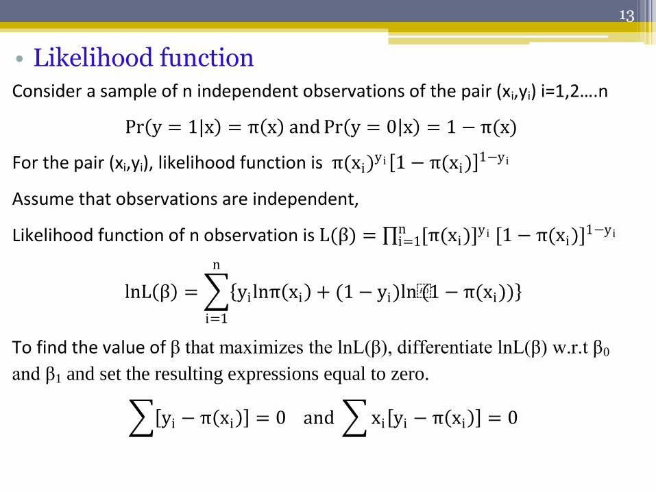
• Likelihood function
13
Consider a sample of n independent observations of the pair (xi,yi) i=1,2….n
Pr y = 1|x = π x and Pr y = 0 x = 1 − π(x)
For the pair (xi,yi), likelihood function is π(xi)y i 1 − π(xi)
1−yi
Assume that observations are independent,
Likelihood function of n observation is L(β) = [π(xi)]y ini=1 [1 − π(xi)]1−yi
lnL β = yilnπ xi + (1 − yi)ln(1 − π(xi))
n
i=1
To find the value of β that maximizes the lnL(β), differentiate lnL(β) w.r.t β0
and β1 and set the resulting expressions equal to zero.
yi − π xi = 0 and xi yi − π xi = 0

• Significance of the CoefficientsUsually involves formulation and testing of a statistical
hypothesis to determine whether the independent variables in the
model are significantly related to the outcome variable.
1. Likelihood ratio test
2. Wald test
14
D = −2ln likelihood of the fitted model
likelihood of the saturated moel = −2 ln likelihood ratio
D is called the deviance.
Let ,G = D(model without the variables) − D(model with the variables)
G = −2ln likelihood without the variable
likelihood with the variable ~xno of extra parameter
2
Wj =βj
SEβ j
~x12

• Score testBased on the slope and expected curvature of the log-
likelihood function L(β) at the null value β0.
• Confidence interval
100(1-α)% C.I for the intercept and slope
• Multiple logistic model
15
u β = ∂L(β)/ ∂β|β0 = u β0
−E[∂2L(β)/ ∂β2|β0] = τ β0
test st: u(β0)/[τ(β0)]1/2 ~N(0,1)
β 0 ± z1−α/2SE β0 and β 1 ± z1−α/2SE β1
𝑔 𝑥 = 𝑙𝑛𝜋(𝑥)
1 − 𝜋(𝑥)= 𝛽0 + 𝛽1𝑥1 + ⋯+ 𝛽𝑝𝑥𝑝
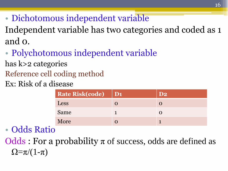
• Dichotomous independent variable
Independent variable has two categories and coded as 1
and 0.
• Polychotomous independent variablehas k>2 categories
Reference cell coding method
Ex: Risk of a disease
• Odds Ratio
Odds : For a probability π of success, odds are defined as
Ω=π/(1-π)
16
Rate Risk(code) D1 D2
Less 0 0
Same 1 0
More 0 1

Independent variable X
Outcome variable(y) X=1 X=0
Y=1
Y=0
Total 1 1
17
π 1 =eβ0+β1
1 + eβ0+β1
𝜋 0 =𝑒𝛽0
1 + 𝑒𝛽0
1 − 𝜋 1 =1
𝑒𝛽0+𝛽1 1 − 𝜋 0 =
1
1 + 𝑒𝛽0
OR =π(1)/[1 − π(1)]
π(0)/[1 − π(0)]= eβ1
95% CI of ln OR = ln(OR) ± 1.96SE[ln OR ]
95% CI of OR = eln(OR )±1.96SE [ln OR ]
• Relative riskRatio of the two outcome probabilities
RR=π(1)/π(0)

LC 50 Value
The concentration of the chemical that kills 50% of the test animals.
Use to compare different chemicals.
In general, the smaller the LC50 value, the more toxic the chemical. The opposite is also true: the larger the LC50 value, the lower the toxicity.
18

• Method of Miller and Tainter
Ex:
The percentage dead for 0 and 100 are corrected before the
determination of probits using following formulas.
For 0%dead = 100(0.25/n)
For 100%dead =100(n-0.25/n)
Fitting linear regression model between log(dose) and probit
value, LC 50 is calculated.
19
Dose Log(dose) % dead Corrected %
Probits
25 1.4 0 2.5 3.04
50 1.7 40 40 4.75
75 1.88 70 70 5.52
100 2 90 90 6.28
150 2.18 100 97.5 6.96

LC50= 57.54mg/kg
• Probit table
20

Application
Laboratory experiment was carried out to evaluate the effect of
different botanicals such as Wara,Keppetiya and Maduruthala in
the control of root knot nematode (M. javanica) by
Prof:(Mrs)W.T.S.D.premachandra, Department Of Zoology.
Approximately 50 juveniles were dispensed into petridishes
containing different concentration extracts (100,80,60,40,20) of
the botanicals. After 48 hours, recorded number of deaths of each
petridishes.
21

Response variable
1 when death is occur
y
0 no death
Independent variables
Concentration
Plant type
22
Plant type D1 D2
Maduruthala 0 0
Keppetiya 1 0
Wara 0 1

• The Logistic Model
23
call:
glm(formula=data$ dead ˜data$Concentration + data$plant.f, family = binomial(link
= ”logit”))
Deviance Residuals:
Min 1Q Median 3Q Max
-2.4779 -0.5636 -0.1515 0.5664 2.5410
Coefficients:
Estimate Std. Error z value Pr(> |z|)
(Intercept) -5.735211 0.131744 -43.53 <2e-16 ***
Concentration 0.063686 0.001481 42.99 <2e-16 ***
Keppetiya 2.388994 0.086474 27.63 <2e-16 ***
Wara 2.702167 0.089134 30.32 <2e-16 ***
Null deviance: 10374.8 on 7499 degrees of freedom
Residual deviance:6350.3 on 7496 degrees of freedom
AIC: 6358.3
Pseduo Rsq= 0.3879

Fitted values
All independent variables are significant.
For every one unit change in concentration, the log odds of death
(versus no death) increases by 0.0636.
Having a death with Keppetiya plant, versus a death with a
Maduruthala plant, changes the log odds of death by 2.3889. And also
Having a death with Wara plant, versus a death with a
Maduruthala plant, changes the log odds of death by 2.7021.
24
π (x) =e−5.735+0.0636Con +2.3889Keppetiya +2.7021Wara
1 + e−5.735+0.0636Con +2.3889Keppetiya +2.7021Wara
Estimated logit,
g x = ln(ODDS) = −5.735 + 0.0636Con + 2.3889Keppetiya + 2.7021Wara

We can test for an overall effect of plant using the Wald test.
Wald test:
test st:= 1036.2 df = 2 P(>X2) = 0.00
The overall effect of plant is statistically significant.
Odds Ratios and their 95%CI:OR 2.5% 97.5%
Intercept 0.003230201 0.002486319 0.00416747
Concentration 1.065757750 1.062704680 1.06889510
Keppetiya 10.902516340 9.215626290 12.93485861
Wara 14.912011210 12.541600465 17.78769387
An increase of one unit in Concentration is associated with 1.0658 increase in
the odds of having a death. Keppetiya increases the odds of having a death
than Maduruthala by 10.903.
25

• The Probit Model
26
call:
glm(formula=data$ dead ˜data$Concentration + data$plant.f, family =
binomial(link = ”probit”))
Deviance Residuals:
Min 1Q Median 3Q Max
-2.5347 -0.5739 -0.1043 0.5857 2.5829
Coefficients:
Estimate Std. Error z value Pr(> |z|)
Intercept -3.2911468 0.0683004 -48.19 <2e-16 ***
Concentration 0.0371691 0.0007816 47.56 <2e-16 ***
Keppetiya 1.3218435 0.0475294 27.81 <2e-16 ***
Wara 1.5192155 0.0486710 31.21 <2e-16 ***
Null deviance:10374.8 on 7499 degrees of freedom
Residual deviance:6346.2 on 7496 degrees of freedom
AIC: 6354.2

The predicted probability of death is
Pr(y=1|x)=π(x)=Φ(−3.2911 + 0.0372Con + 1.3218Keppetiya +
1.5192Wara)
All independent variables are significance and has positive effect
from each variables.
For every one unit change of Concentration, the c.d.f of standard
normal distribution is increase by 0.0372.
Having a death with Keppetiya plant, versus a death with a
Maduruthala plant, changes c.d.f of death by 1.3218.
Having a death with Wara plant, versus a death with a
Maduruthala plant, changes c.d.f of death by 1.5192.
27

• Marginal effects
Probability of having a death changes by 0.88% for
every one unit change of Concentration.
Having a death in Keppetiya is 31.3% more likely than
in Maduruthala.
And also
Having a death in Wara is 35.98% more likely than
in Maduruthala.
28
Concentration Keppetiya Wara
0.008802969 0.313060054 0.359804831

• Comparison of LC50 values
Lowest LC50 value means that highest effect on death.
Wara plants extract has the lowest LC50 value.
29
Plant LC50 using Logit
model
LC50 using probit
model
Maduruthala 90.1729 88.4704
Keppetiya 52.6116 52.9382
Wara 47.6871 47.6317

The maximal response has been obtained
by Wara plant extract.
That is,
it has highest efficacy than others. Potency of
Wara is also highest value but no more
differ from Keppetiya.
Maduruthala plant extract has shown
lower potency and lower efficacy.
30

• Conclusions
According to the LC50 values and other toxic
measures , Wara is recommended as the effective
botanical than other botanicals.
Also,
It is enough, add 47.63mg/ml of Wara plant extract to
kill 50% of the Nematode population.
31

Bibliography[1]Razzaghi:Journal of Modern Applied Statistical Methods,BloomsburgUniversity,May 2013, Vol. 12, No. 1, 164-169.
[2] Weng KeeWong,Peter A. Lachenbruch:Tutorial in Biostatistic and Designing
studies for dose response,VOL.15,343-359(1996).
[3] Susan Ma:LC50 Sediment Testing of the Insecticide Fipronil with the Non-Target
Organism,May 8 2006.
[4] Muhammad Akram Randhawa: http://www.ayubmed.edu.pk/JAMC/ PAST/21-3/ Randhawa,College of Medicine, University of Dammam: 2009;21(3).
[5] K. Bondari:Paper ST01,University of Georgia, Tifton,GA 31793-0748.
32
[6] Park, Hun Myoung:Regression models for binary dependent variables using
Stata, SAS, R, LIMDEP, and SPSS,Indiana University(2009).
[7] Probit Analysis By: Kim Vincent
[8] Mark Tranmer,Mark Elliot:Binary Logistic Regression
[9] DavidW. Hosmer,JR.,Stanley Lemeshow,Rodney X. Sturdivant:Applied Lo-
gistic Regression,Third Edition,ISBN 978-0-470-58247-3.
[10] Scott A. Czepiel:Maximum Likelihood Estimation of Logistic Regression Mod-
els,Theory and Implementation.
[11] Park, Hyeoun-Ae:An Introduction to Logistic Regression,Seoul National Uni-
versity,Korea,J Korean Acad Nurs Vol.43 No.2,April 2013.
[12] Finney, D. J., Ed. (1952). Probit Analysis,Cambridge, England, Cambridge
University Press.
33

34


