62
Problem Reduction & Game Playing Lecture Module 7
| Date post: | 01-Jan-2016 |
| Category: |
Documents |
| Upload: | uma-hodges |
| View: | 195 times |
| Download: | 21 times |
Problem Reduction & Game Playing
Lecture Module 7
Problem Reduction
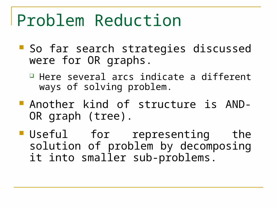
So far search strategies discussed were for OR graphs. Here several arcs indicate a different ways of
solving problem.
Another kind of structure is AND-OR graph (tree).
Useful for representing the solution of problem by decomposing it into smaller sub-problems.
Problem Reduction – Contd..
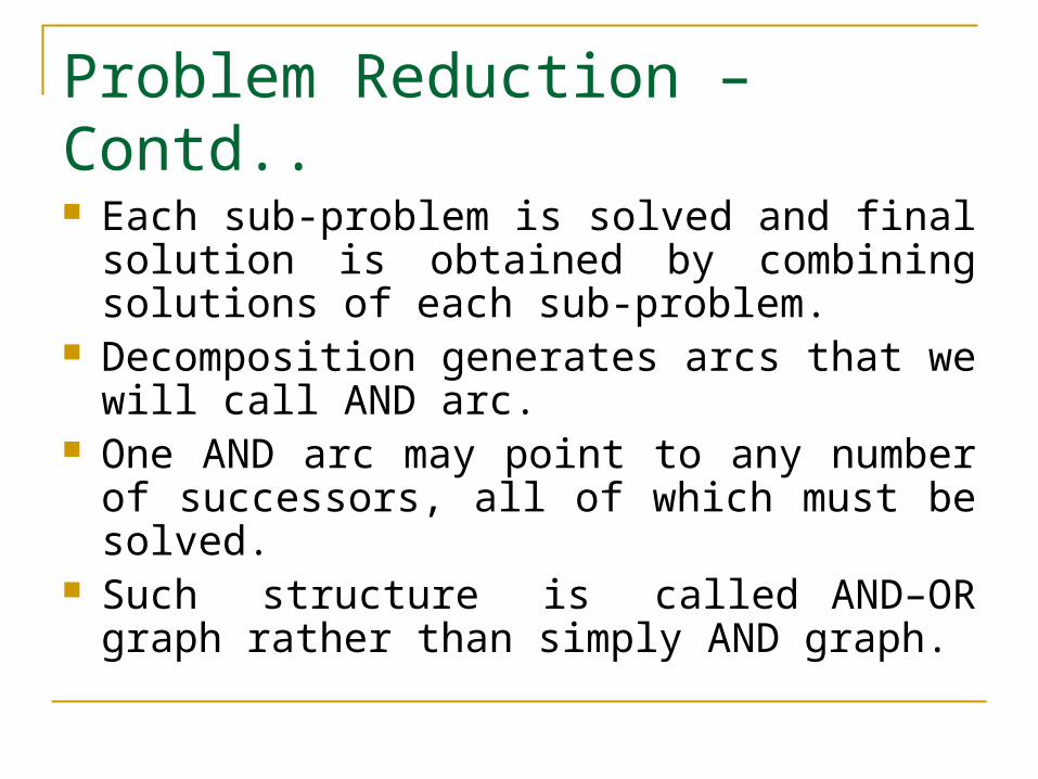
Each sub-problem is solved and final solution is obtained by combining solutions of each sub-problem.
Decomposition generates arcs that we will call AND arc.
One AND arc may point to any number of successors, all of which must be solved.
Such structure is called AND–OR graph rather than simply AND graph.
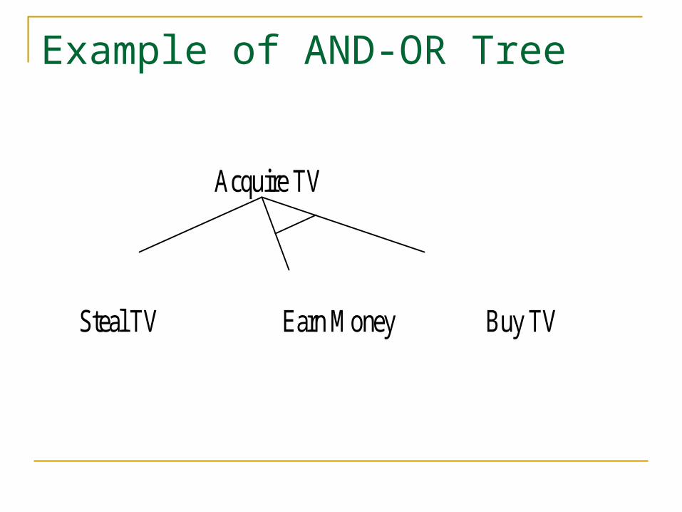
Example of AND-OR Tree
Acquire TV
Steal TV Earn Money Buy TV
AND–OR Graph
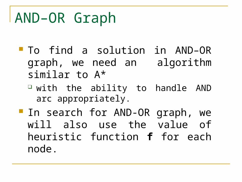
To find a solution in AND–OR graph, we need an algorithm similar to A* with the ability to handle AND arc
appropriately. In search for AND-OR graph, we will also
use the value of heuristic function f for each node.
AND–OR Graph Search
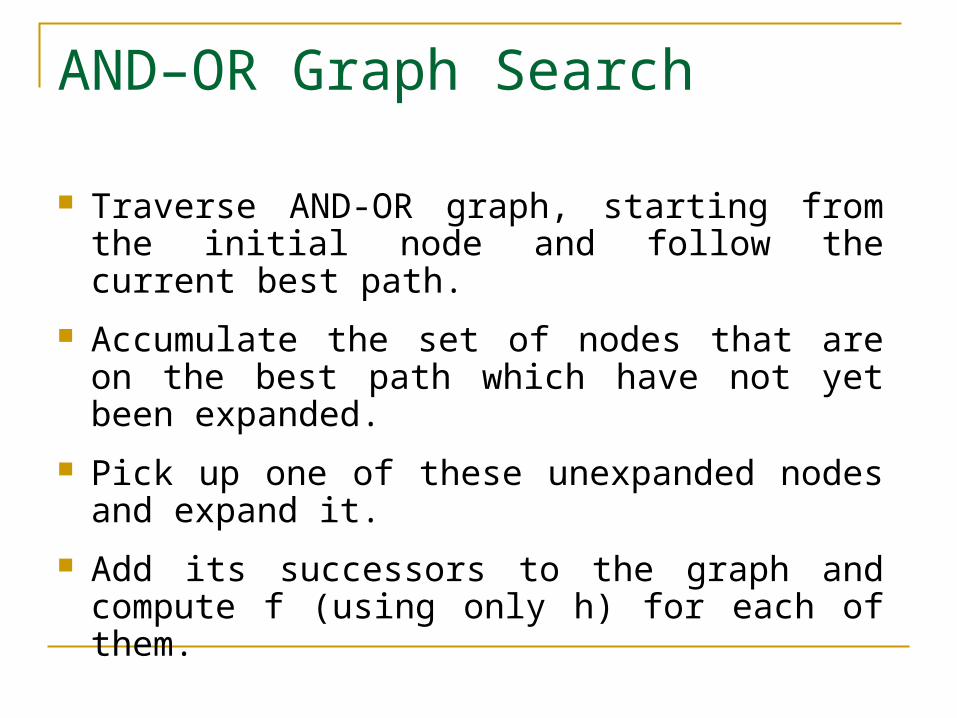
Traverse AND-OR graph, starting from the initial node and follow the current best path.
Accumulate the set of nodes that are on the best path which have not yet been expanded.
Pick up one of these unexpanded nodes and expand it.
Add its successors to the graph and compute f (using only h) for each of them.
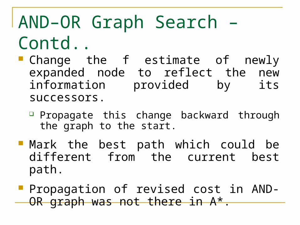
AND–OR Graph Search – Contd.. Change the f estimate of newly expanded node
to reflect the new information provided by its successors. Propagate this change backward through the graph to
the start.
Mark the best path which could be different from the current best path.
Propagation of revised cost in AND-OR graph was not there in A*.
Contd.. Example
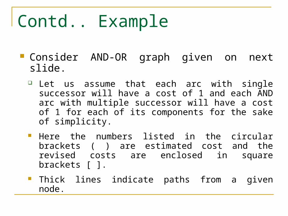
Consider AND-OR graph given on next slide. Let us assume that each arc with single successor will
have a cost of 1 and each AND arc with multiple successor will have a cost of 1 for each of its components for the sake of simplicity.
Here the numbers listed in the circular brackets ( ) are estimated cost and the revised costs are enclosed in square brackets [ ].
Thick lines indicate paths from a given node.
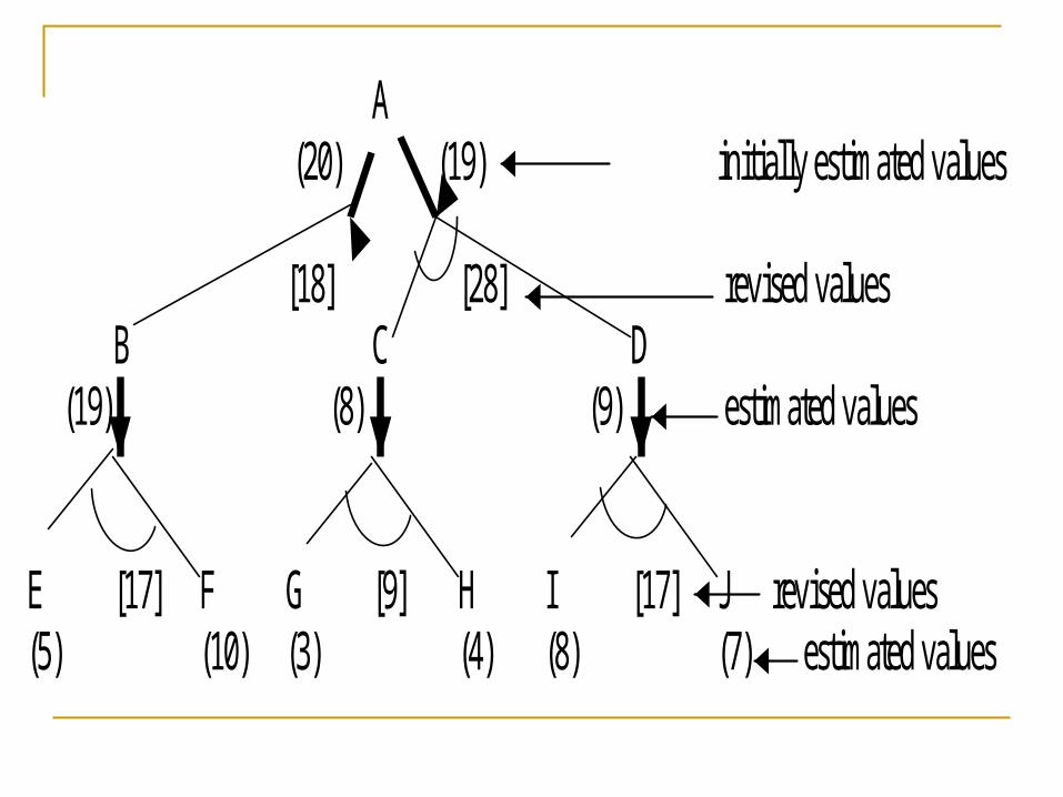
A (20) (19) initially estimated values [18] [28] revised values B C D (19) (8) (9) estimated values E [17] F G [9] H I [17] J revised values (5) (10) (3) (4) (8) (7) estimated values
Explanation
Initially we start from start node A and compute heuristic values for each of its successors, say {B, (C and D)} as {19, (8, 9)}.
The estimated cost of paths from A to B is 20 (19 + cost of one arc from A to B) and from A to (C and D) path is 19 ( 8+9 + cost of two arcs A to C and A to D).
The path from A to (C and D) seems to be better. So expend this AND path by expending C to {(G and H)} and D to {(I and J)}.
Contd..
Now heuristic values of G, H, I and J are 3, 4, 8 and 7 respectively.
This leads to revised cost of C and D as 9 and 17 respectively.
These values are propagated up and the revised costs of path from A through (C and D) is calculated as 28 (9 + 17 + cost of arcs A to C and A to D).
Now the revised cost of this path is 28 instead of earlier estimation of 19 and this path is no longer a best path.
Contd.. Then choose path from A to B for expansion.
After expansion we see that heuristic value of node B is 17 thus making cost of path from A to B to be 18.
This path is still best path so far, so further explore path from A to B.
The process continues until either a solution is found or all paths have lead to dead ends, indicating that there is no solution.
Cyclic Graph
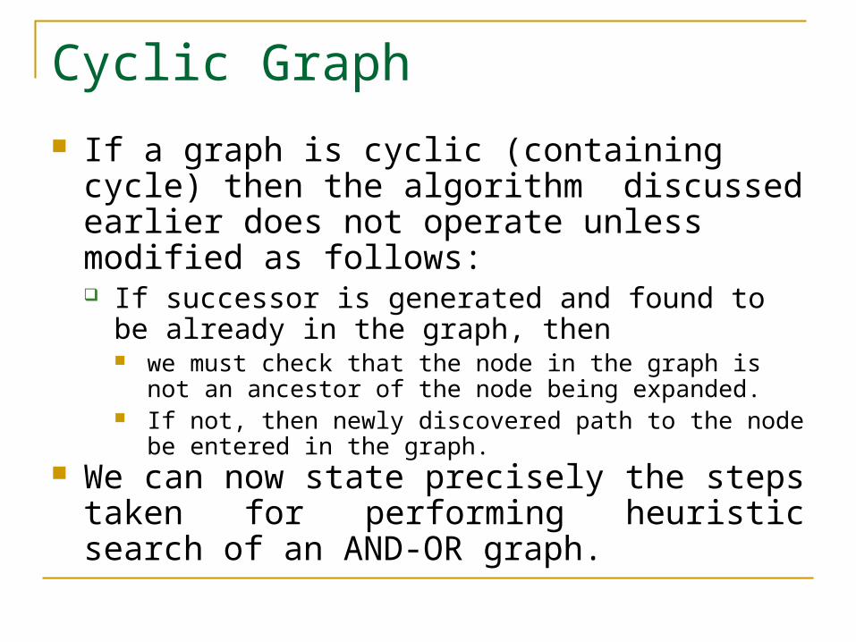
If a graph is cyclic (containing cycle) then the algorithm discussed earlier does not operate unless modified as follows: If successor is generated and found to be already in
the graph, then we must check that the node in the graph is not an ancestor of
the node being expanded. If not, then newly discovered path to the node be entered in
the graph. We can now state precisely the steps taken for
performing heuristic search of an AND-OR graph.

Cyclic Graph – Contd..
Algorithm for searching AND-OR graph is called AO* Here we maintain single structure G, representing the
part of the search graph explicitly generated so far rather than two lists, OPEN and CLOSED as in previous algorithms.
Each node in the graph will point both down to its immediate successors and up to
its immediate predecessor. have an h value (an estimate of the cost of a path
from current node to a set of solution nodes) associated with it.
Cyclic Graph – Contd..
We will not store g (cost from start to current node) as it is not possible to compute a single such value since there may be many paths to the same state. The value g is also not necessary because of the
top-down traversing of the best-known path which guarantees that only nodes on the best path will ever be considered for expansion.
So h will be good estimate for AND/OR graph search.
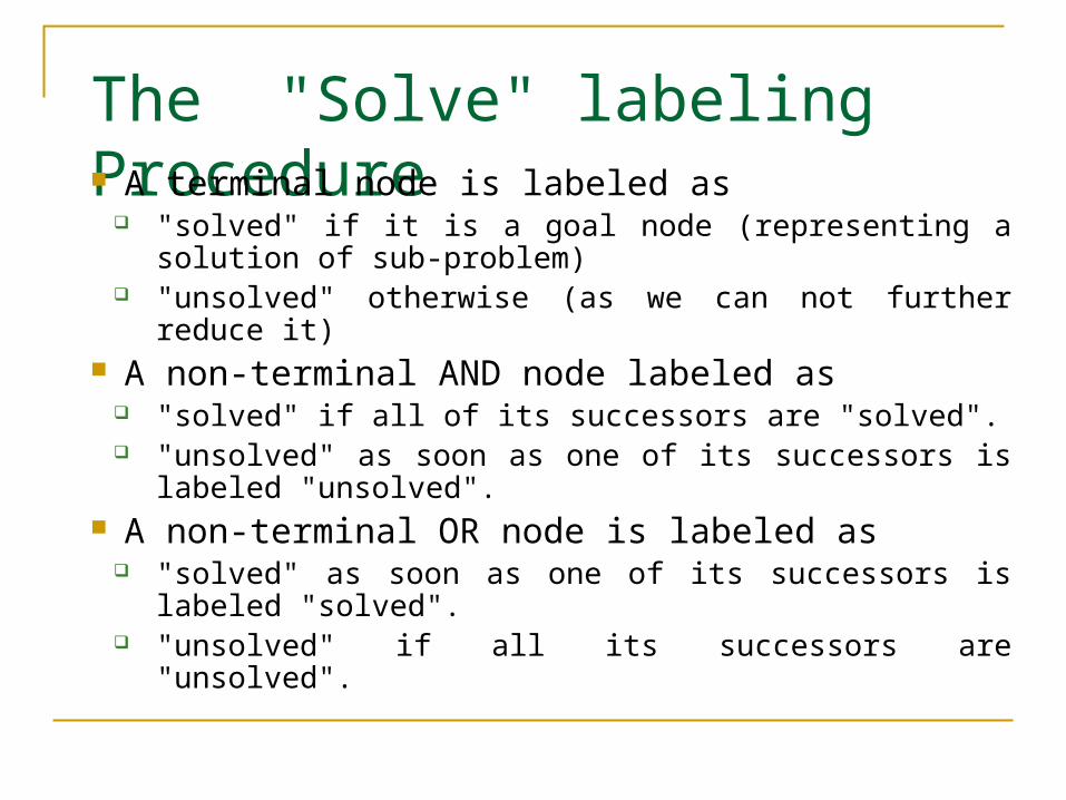
The "Solve" labeling Procedure A terminal node is labeled as
"solved" if it is a goal node (representing a solution of sub-problem)
"unsolved" otherwise (as we can not further reduce it) A non-terminal AND node labeled as
"solved" if all of its successors are "solved". "unsolved" as soon as one of its successors is
labeled "unsolved". A non-terminal OR node is labeled as
"solved" as soon as one of its successors is labeled "solved".
"unsolved" if all its successors are "unsolved".
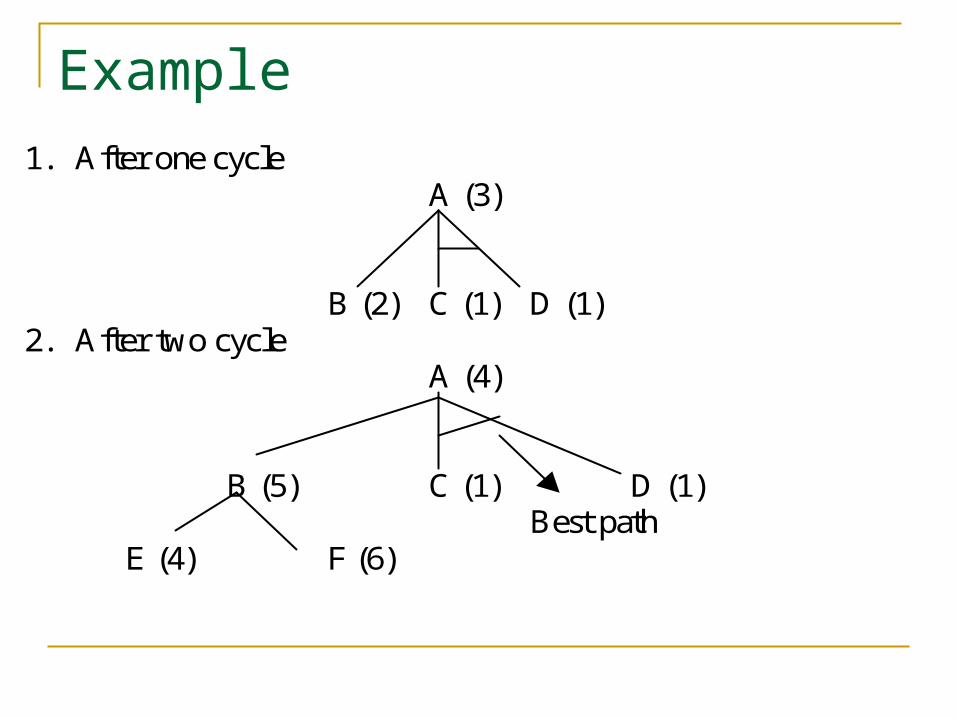
Example1. After one cycle
A (3)
B (2) C (1) D (1)2. After two cycle
A (4)
B (5) C (1) D (1)Best path
E (4) F (6)
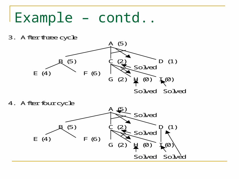
Example – contd..3. After three cycle
A (5)
B (5) C (2) D (1)Solved
E (4) F (6)G (2) H (0) I (0)
Solved Solved
4. After four cycleA (5)
Solved
B (5) C (2) D (1)Solved
E (4) F (6)G (2) H (0) I (0)
Solved Solved
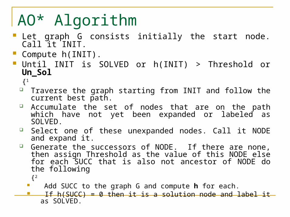
AO* Algorithm Let graph G consists initially the start node. Call it INIT. Compute h(INIT). Until INIT is SOLVED or h(INIT) > Threshold or Un_Sol
{1
Traverse the graph starting from INIT and follow the current best path.
Accumulate the set of nodes that are on the path which have not yet been expanded or labeled as SOLVED.
Select one of these unexpanded nodes. Call it NODE and expand it.
Generate the successors of NODE. If there are none, then assign Threshold as the value of this NODE else for each SUCC that is also not ancestor of NODE do the following {2
Add SUCC to the graph G and compute h for each. If h(SUCC) = 0 then it is a solution node and label it as
SOLVED.
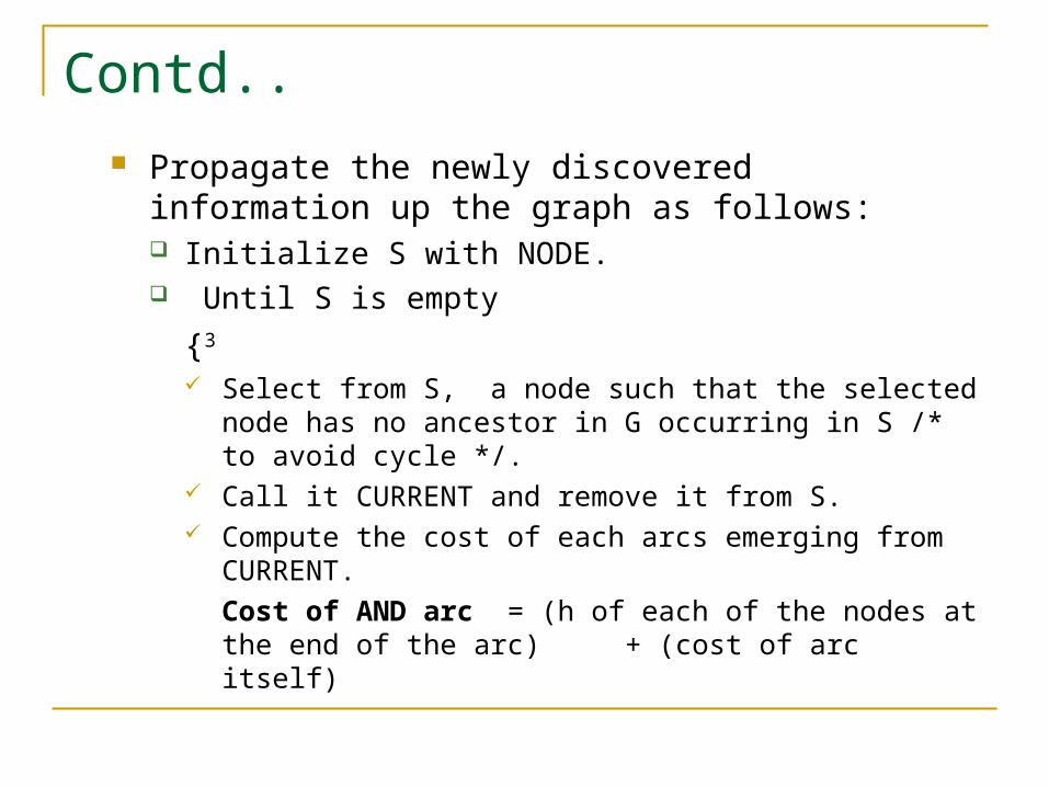
Contd.. Propagate the newly discovered information up the
graph as follows: Initialize S with NODE. Until S is empty
{3
Select from S, a node such that the selected node has no ancestor in G occurring in S /* to avoid cycle */.
Call it CURRENT and remove it from S. Compute the cost of each arcs emerging from CURRENT.
Cost of AND arc = (h of each of the nodes at the end of the arc) + (cost of arc itself)
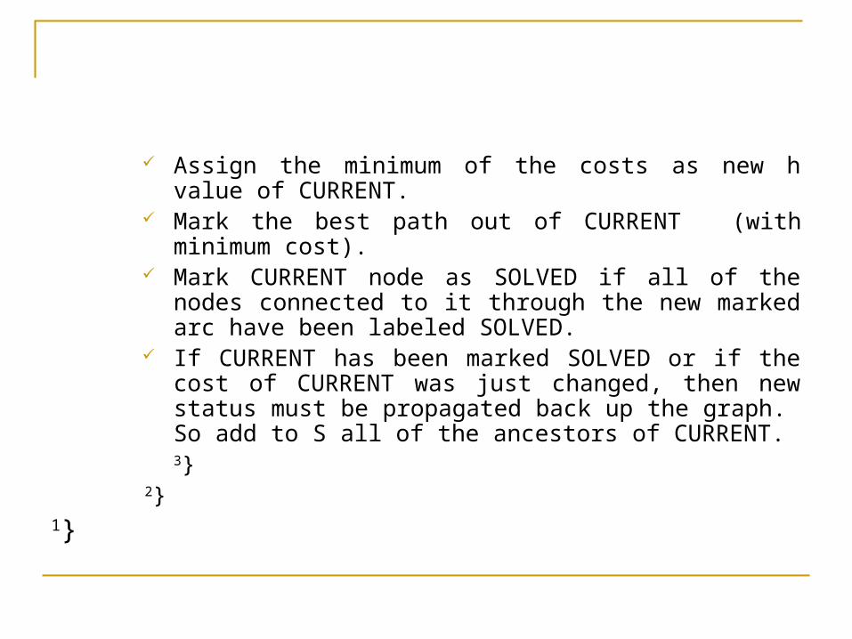
Assign the minimum of the costs as new h value of CURRENT.
Mark the best path out of CURRENT (with minimum cost).
Mark CURRENT node as SOLVED if all of the nodes connected to it through the new marked arc have been labeled SOLVED.
If CURRENT has been marked SOLVED or if the cost of CURRENT was just changed, then new status must be propagated back up the graph. So add to S all of the ancestors of CURRENT.3}
2}1}
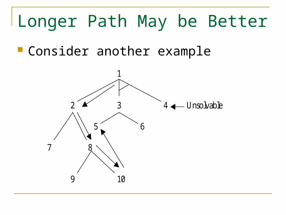
Longer Path May be Better
Consider another example
1
2 3 4 Unsolvable
5 6
7 8
9 10
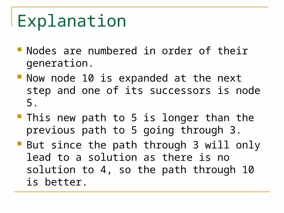
Explanation
Nodes are numbered in order of their generation.
Now node 10 is expanded at the next step and one of its successors is node 5.
This new path to 5 is longer than the previous path to 5 going through 3.
But since the path through 3 will only lead to a solution as there is no solution to 4, so the path through 10 is better.
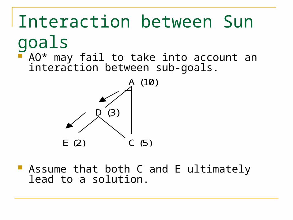
Interaction between Sun goals AO* may fail to take into account an interaction
between sub-goals.
Assume that both C and E ultimately lead to a solution.
A (10)
D (3)
E (2) C (5)
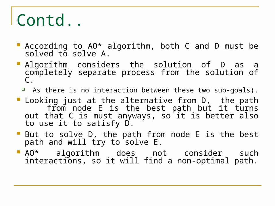
Contd.. According to AO* algorithm, both C and D must be
solved to solve A. Algorithm considers the solution of D as a
completely separate process from the solution of C. As there is no interaction between these two sub-goals).
Looking just at the alternative from D, the path from node E is the best path but it turns out that C is must anyways, so it is better also to use it to satisfy D.
But to solve D, the path from node E is the best path and will try to solve E.
AO* algorithm does not consider such interactions, so it will find a non-optimal path.
Game Playing Games require different search procedures. Basically they are based on generate and test philosophy. The generator generates individual move in the search
space, each of which is then evaluated by the tester and the most promising one is chosen.
Game playing is most practical and direct application of the heuristic search problem solving paradigm.
It is clear that to improve the effectiveness of a search for problem solving programs, there are two things that can be done: Improve the generate procedure so that only good moves
(paths) are generated. Improve the test procedure so that the best moves (paths)
will be recognized and explored first.
Contd… Let us consider only two player discrete, perfect
information games, such as tic-tac-toe, chess, checkers etc. Discrete because they contain finite number of states
or configurations. Perfect-information because both players have
access to the same information about the game in progress (card games are not perfect - information games).
Two-player games are easier to imagine & think and more common to play.
Typical characteristic of the games is to ‘look ahead’ at future positions in order to succeed.
Correspondence with State Space
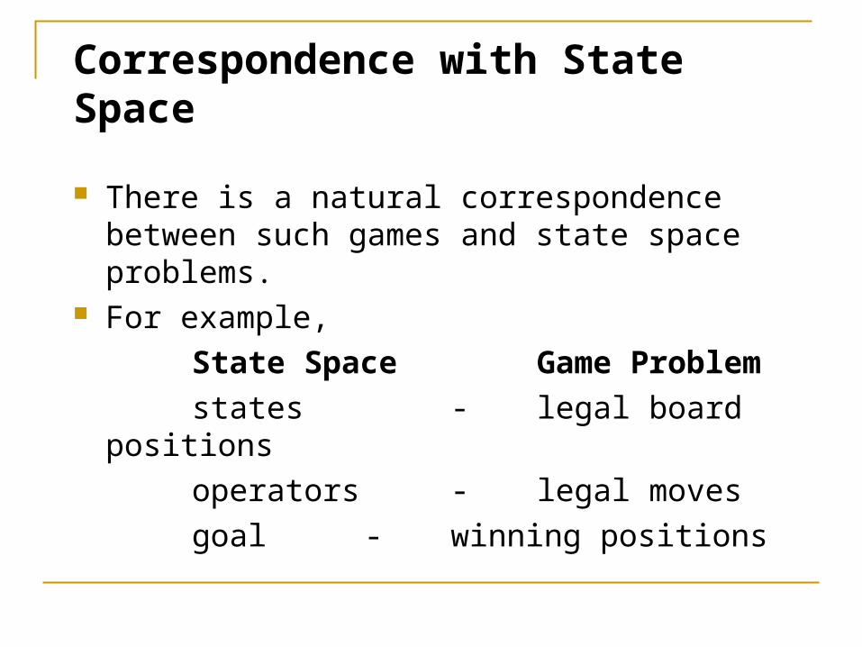
There is a natural correspondence between such games and state space problems.
For example,
State Space Game Problem
states - legal board positions
operators - legal moves
goal - winning positions
Contd… The game begins from a specified initial state and ends in
position that can be declared win for one, loss for other or possibly a draw.
Game tree is an explicit representation of all possible plays of the game. The root node is an initial position of the game. Its successors are the positions that the first player can
reach in one move, and Their successors are the positions resulting from the second
player's replies and so on. Terminal or leaf nodes are represented by WIN, LOSS or
DRAW. Each path from the root to a terminal node represents a
different complete play of the game.
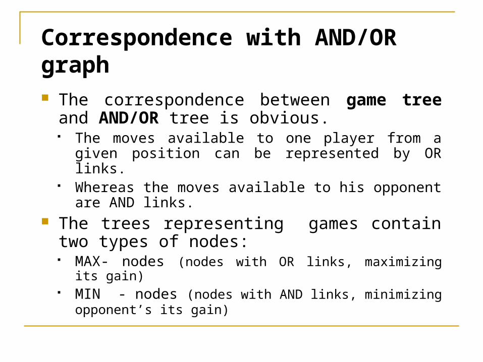
Correspondence with AND/OR graph The correspondence between game tree and
AND/OR tree is obvious. The moves available to one player from a given position
can be represented by OR links. Whereas the moves available to his opponent are AND
links. The trees representing games contain two types
of nodes: MAX- nodes (nodes with OR links, maximizing its gain) MIN - nodes (nodes with AND links, minimizing opponent’s
its gain)
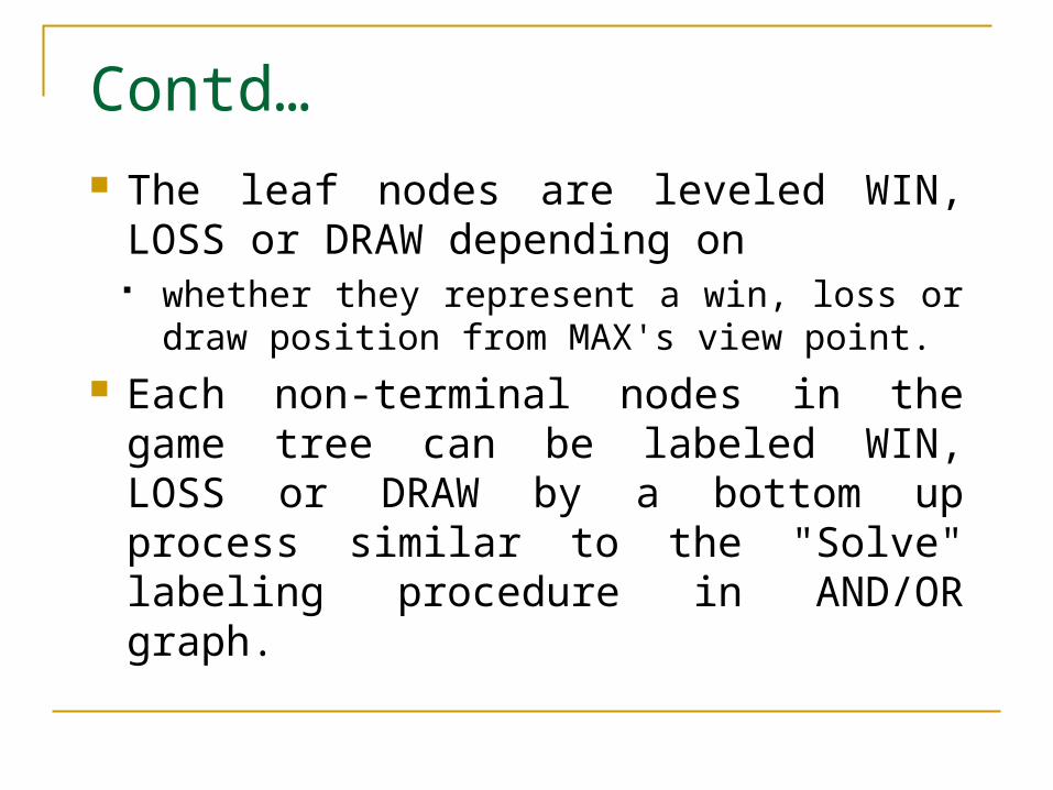
Contd… The leaf nodes are leveled WIN, LOSS or
DRAW depending on whether they represent a win, loss or draw
position from MAX's view point. Each non-terminal nodes in the game tree
can be labeled WIN, LOSS or DRAW by a bottom up process similar to the "Solve" labeling procedure in AND/OR graph.
Status Labeling Procedure
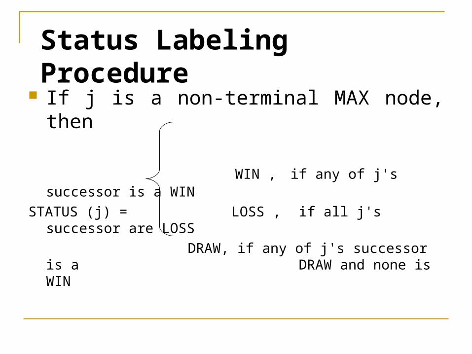
If j is a non-terminal MAX node, then
WIN , if any of j's successor is a WIN
STATUS (j) = LOSS , if all j's successor are LOSS
DRAW, if any of j's successor is a DRAW and none is WIN
Contd…
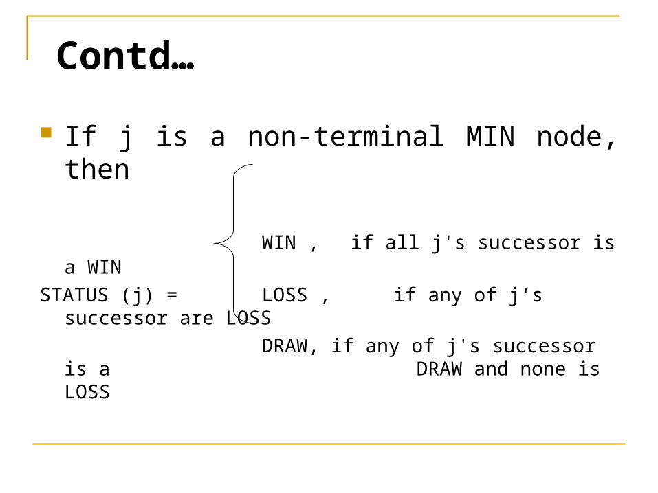
If j is a non-terminal MIN node, then
WIN , if all j's successor is a WIN
STATUS (j) = LOSS , if any of j's successor are LOSS
DRAW, if any of j's successor is a DRAW and none is LOSS
Contd… The function STATUS(j) should be interpreted as the
best terminal status MAX can achieve from position j, if MAX plays optimally against a perfect opponent.
Example: Consider a game tree on next slide. Let us denote
• MAX X • MIN Y, • WIN W, • DRAW D and • LOSS L.
The status of the leaf nodes is assigned by the rules of the game whereas, those of non-terminal nodes are determined by the labeling procedure.
Solving a game tree means labeling the root node by WIN, LOSS, or DRAW from Max player point of view.
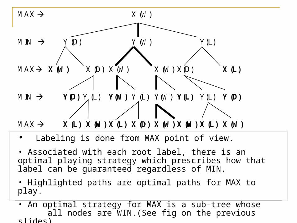
MAX X (W) MIN Y (D) Y (W) Y(L) MAX X (W) X (D) X (W) X (W) X(D) X (L) MIN Y(D) Y (L) Y(W) Y (L) Y(W) Y(L) Y(L) Y (D) MAX X (L) X (W) X (L) X (D) X (W) X (W) X (L) X (W)
• Labeling is done from MAX point of view.
• Associated with each root label, there is an optimal playing strategy which prescribes how that label can be guaranteed regardless of MIN.
• Highlighted paths are optimal paths for MAX to play.
• An optimal strategy for MAX is a sub-tree whose all nodes are WIN.(See fig on the previous slides)
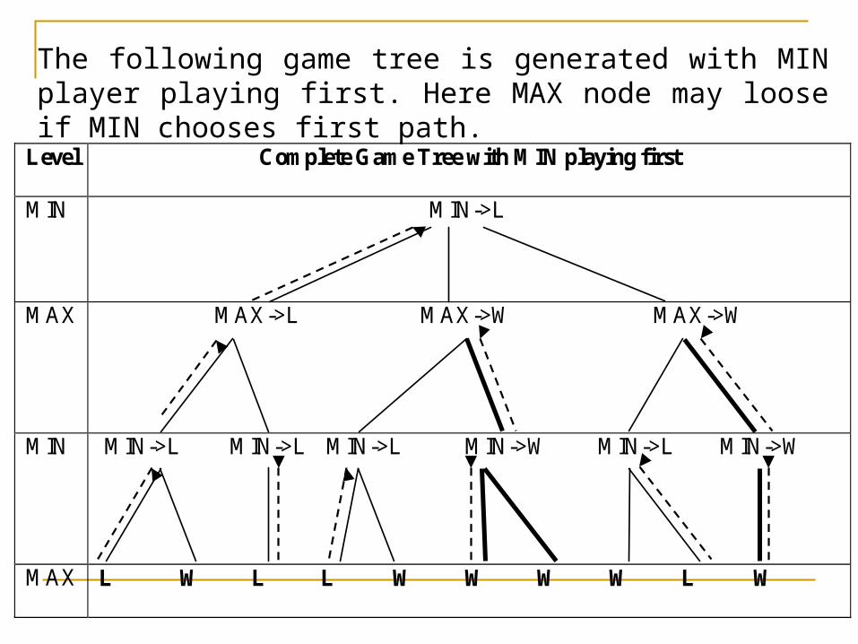
Level Complete Game Tree with MIN playing first
MIN
MIN->L
MAX
MAX->L MAX->W MAX->W
MIN
MIN->L MIN->L MIN->L MIN->W MIN->L MIN->W
MAX
L W L L W W W W L W
The following game tree is generated with MIN player playing first. Here MAX node may loose if MIN chooses first path.
Look-ahead Strategy The status labeling procedure described
earlier requires that a complete game tree or at least sizable portion of it be generated.
For most of the games, tree of possibilities is far too large to be generated and evaluated backward from the terminal nodes in order to determine the optimal first move.
Examples: Checkers : Non-terminal nodes are 1040 and 1021
centuries required if 3 billion nodes could be generated each second.
Chess : 10120 nodes and 10101 centuries. So this approach is not practical
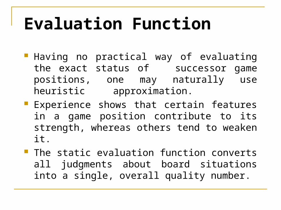
Evaluation Function
Having no practical way of evaluating the exact status of successor game positions, one may naturally use heuristic approximation.
Experience shows that certain features in a game position contribute to its strength, whereas others tend to weaken it.
The static evaluation function converts all judgments about board situations into a single, overall quality number.
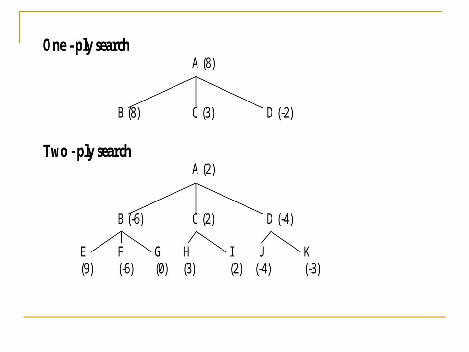
One - ply search A (8) B (8) C (3) D (-2)
Two - ply search
A (2) B (-6) C (2) D (-4)
E F G H I J K (9) (-6) (0) (3) (2) (-4) (-3)
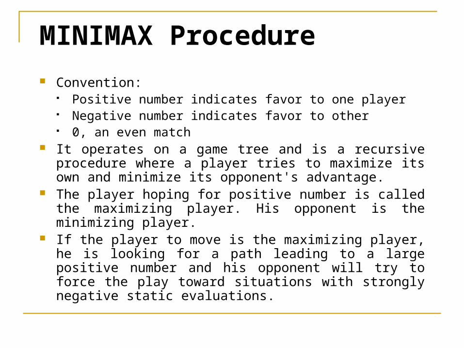
MINIMAX Procedure Convention:
Positive number indicates favor to one player Negative number indicates favor to other 0, an even match
It operates on a game tree and is a recursive procedure where a player tries to maximize its own and minimize its opponent's advantage.
The player hoping for positive number is called the maximizing player. His opponent is the minimizing player.
If the player to move is the maximizing player, he is looking for a path leading to a large positive number and his opponent will try to force the play toward situations with strongly negative static evaluations.
Values are backed up to the starting position.
The procedure by which the scoring information passes up the game tree is called the MINIMAX procedure
The score at each node is either minimum or maximum of the scores at the nodes immediately below.
It is a depth-first, depth limited search procedure.
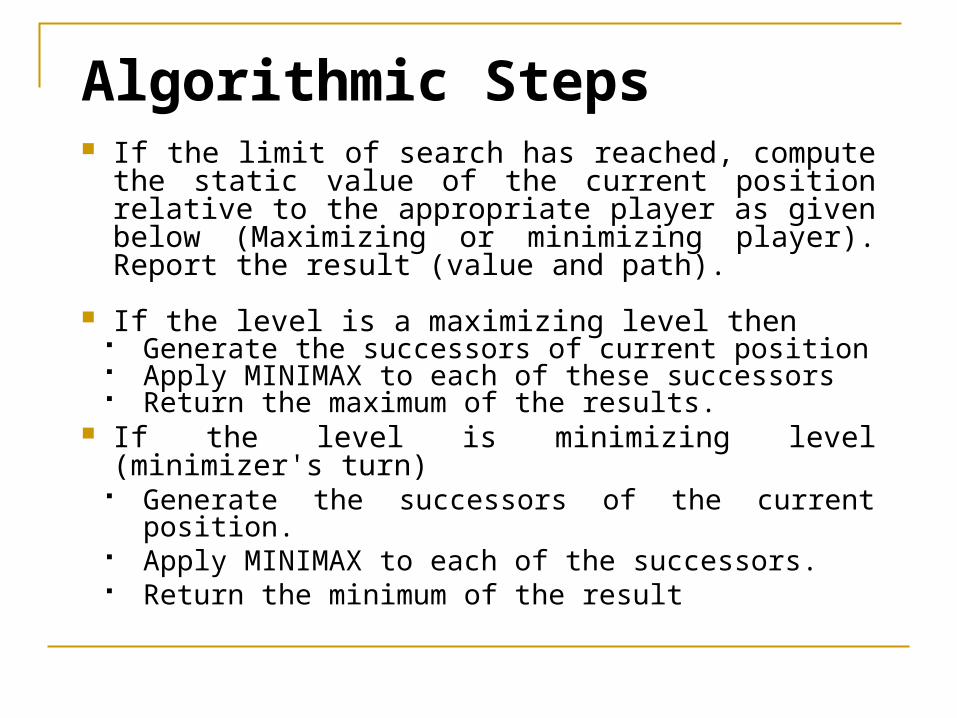
Algorithmic Steps If the limit of search has reached, compute the
static value of the current position relative to the appropriate player as given below (Maximizing or minimizing player). Report the result (value and path).
If the level is a maximizing level then Generate the successors of current position Apply MINIMAX to each of these successors Return the maximum of the results.
If the level is minimizing level (minimizer's turn) Generate the successors of the current position. Apply MINIMAX to each of the successors. Return the minimum of the result
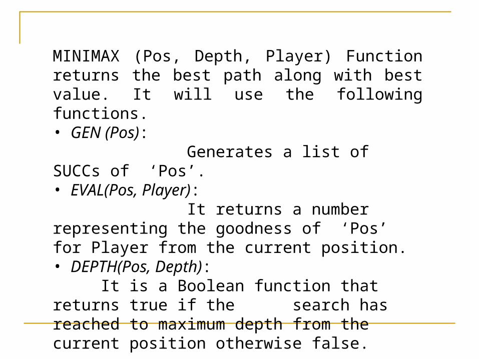
MINIMAX (Pos, Depth, Player) Function returns the best path along with best value. It will use the following functions.• GEN (Pos): Generates a list of SUCCs of ‘Pos’.• EVAL(Pos, Player): It returns a number representing the goodness of
‘Pos’ for Player from the current position.• DEPTH(Pos, Depth):
It is a Boolean function that returns true if the search has reached to maximum depth from the current position otherwise false.
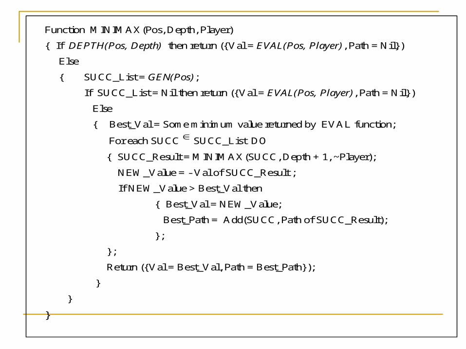
Function MINIMAX(Pos, Depth, Player)
{ If DEPTH(Pos, Depth) then return ({Val = EVAL(Pos, Player), Path = Nil})
Else
{ SUCC_List = GEN(Pos);
If SUCC_List = Nil then return ({Val = EVAL(Pos, Player), Path = Nil})
Else
{ Best_Val = Some minimum value returned by EVAL function;
For each SUCC SUCC_List DO
{ SUCC_Result = MINIMAX(SUCC, Depth + 1, ~Player);
NEW_Value = - Val of SUCC_Result ;
If NEW_Value > Best_Val then
{ Best_Val = NEW_Value;
Best_Path = Add(SUCC, Path of SUCC_Result);
};
};
Return ({Val = Best_Val, Path = Best_Path});
}
}
}
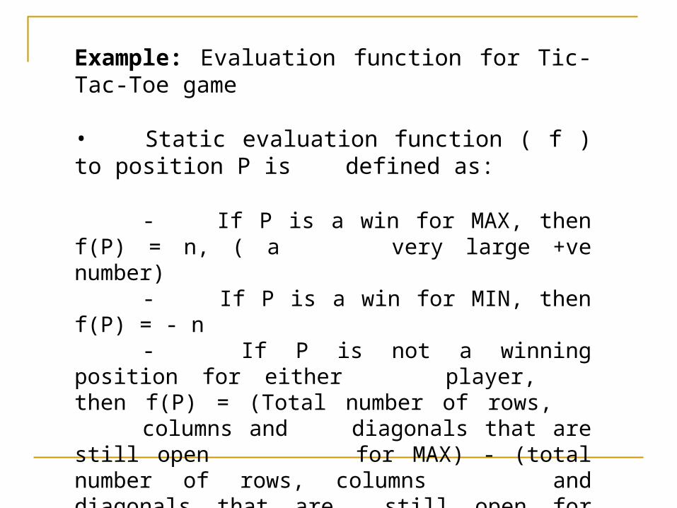
Example: Evaluation function for Tic-Tac-Toe game
• Static evaluation function ( f ) to position P is defined as:
- If P is a win for MAX, then f(P) = n, ( a very large +ve number)
- If P is a win for MIN, then f(P) = - n- If P is not a winning position for either
player, then f(P) = (Total number of rows, columns and diagonals that are still open for MAX) - (total number of rows, columns and diagonals that are still open for MIN)
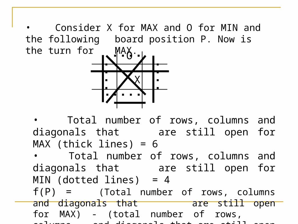
O
X • Total number of rows, columns and diagonals that are still open for MAX (thick lines) = 6• Total number of rows, columns and diagonals that are still open for MIN (dotted lines) = 4f(P) = (Total number of rows, columns and diagonals that
are still open for MAX) - (total number of rows, columns and diagonals that are still open for MIN) = 2
• Consider X for MAX and O for MIN and the following board position P. Now is the turn for MAX.
Remarks:
• Since the MINIMAX procedure is a depth-first process, the efficiency can often be improved by using dynamic branch-and-bound technique in which partial solutions that are clearly worse
than known solutions can be abandoned.
• Further, there is another procedure that reduces- the number of tree branches to be explored and
- the number of static evaluation to be applied.
• This strategy is called Alpha-Beta pruning.
Alpha-Beta Pruning
It requires the maintenance of two threshold values. One representing a lower bound () on the value
that a maximizing node may ultimately be assigned (we call this alpha) and
Another representing upper bound () on the value that a minimizing node may be assigned (we call it beta).
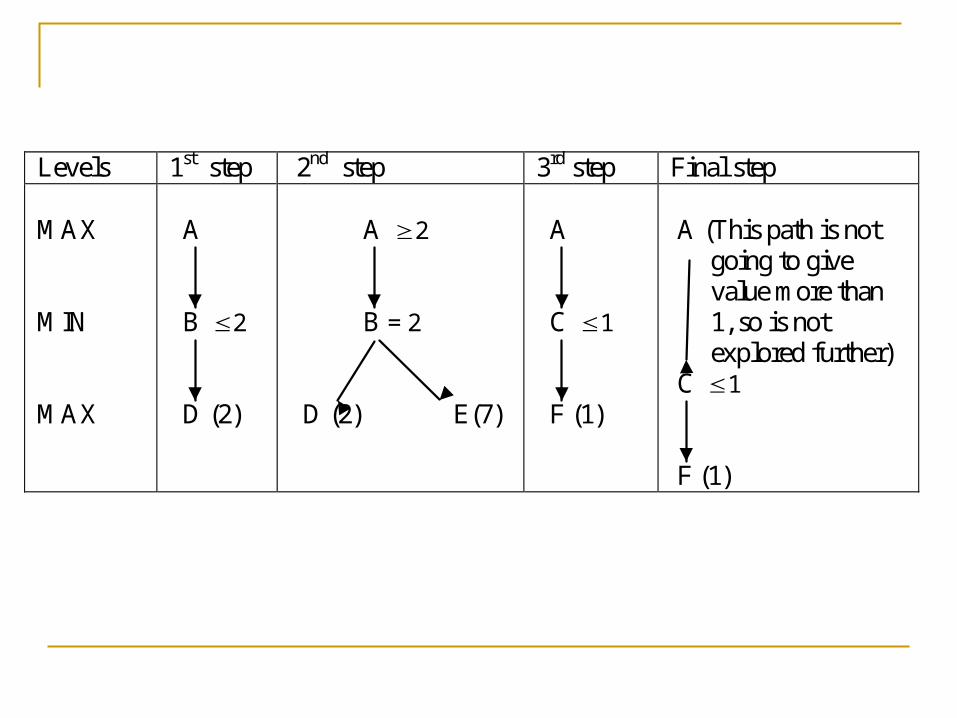
Levels 1st step 2nd step 3rd step Final step MAX MIN MAX
A B 2 D (2)
A 2 B = 2 D (2) E(7)
A C 1 F (1)
A (This path is not going to give value more than 1, so is not explored further) C 1 F (1)
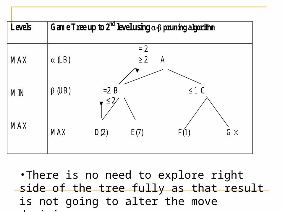
Levels Game Tree up to 2nd level using - pruning algorithm
MAX MIN MAX
= 2 (LB) ≥ 2 A
(UB) =2 B ≤ 1 C ≤ 2 MAX D(2) E(7) F(1) G
•There is no need to explore right side of the tree fully as that result is not going to alter the move decision.
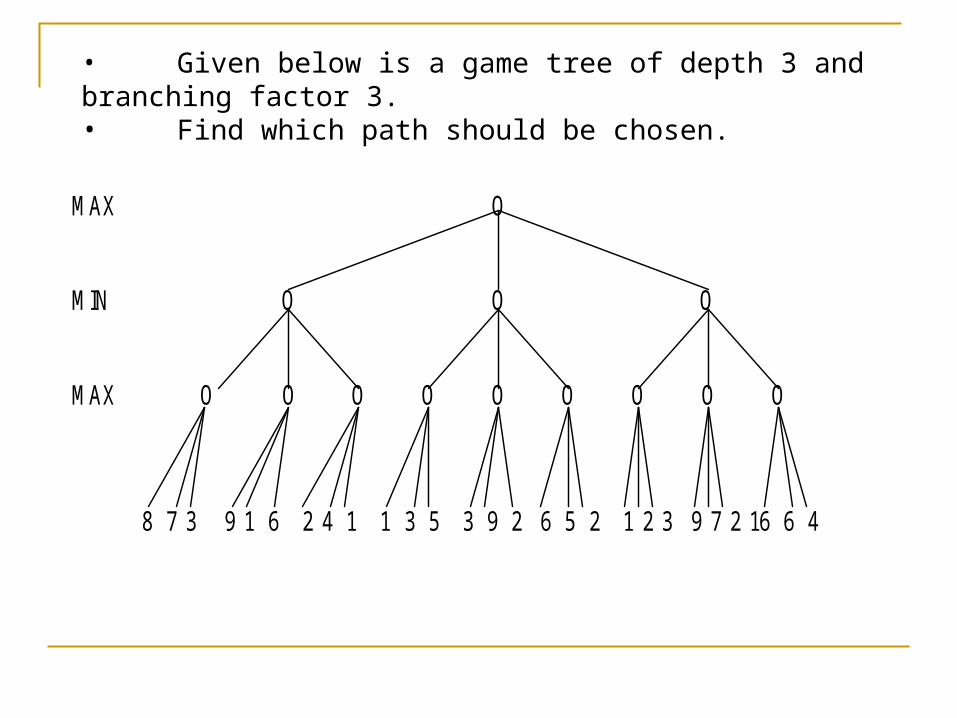
MAX O MIN O O O MAX O O O O O O O O O
8 7 3 9 1 6 2 4 1 1 3 5 3 9 2 6 5 2 1 2 3 9 7 2 16 6 4
• Given below is a game tree of depth 3 and branching factor 3. • Find which path should be chosen.
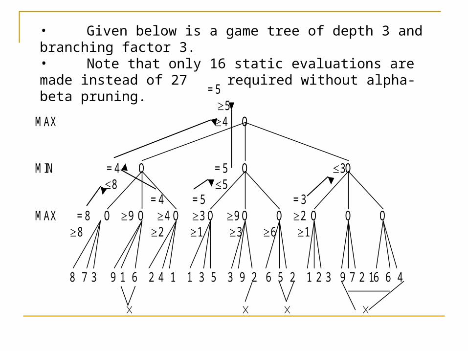
= 5 5 MAX 4 O MIN = 4 O = 5 O 3 O 8 5 = 4 = 5 = 3 MAX = 8 O 9 O 4 O 3 O 9 O O 2 O O O
8 2 1 3 6 1 8 7 3 9 1 6 2 4 1 1 3 5 3 9 2 6 5 2 1 2 3 9 7 2 16 6 4
• Given below is a game tree of depth 3 and branching factor 3. • Note that only 16 static evaluations are made instead of 27 required without alpha-beta pruning.
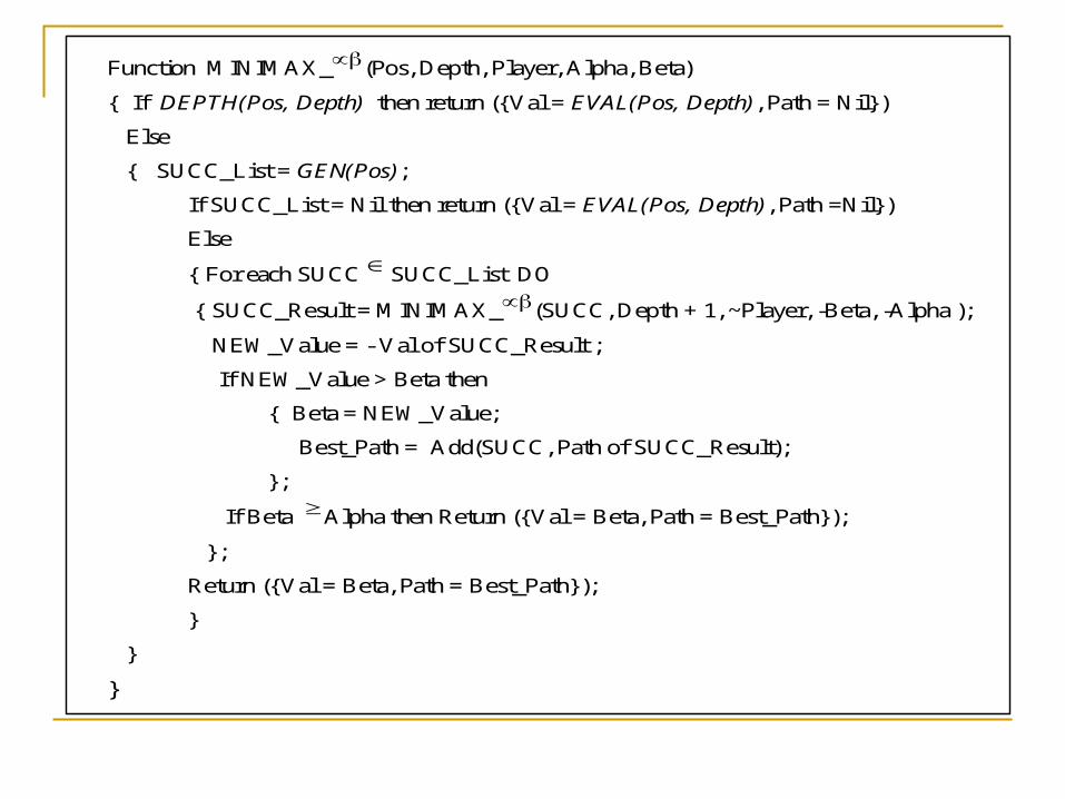
Function MINIMAX_(Pos, Depth, Player, Alpha, Beta)
{ If DEPTH(Pos, Depth) then return ({Val = EVAL(Pos, Depth), Path = Nil})
Else
{ SUCC_List = GEN(Pos);
If SUCC_List = Nil then return ({Val = EVAL(Pos, Depth), Path =Nil})
Else
{ For each SUCC SUCC_List DO
{ SUCC_Result = MINIMAX_(SUCC, Depth + 1, ~Player, -Beta, -Alpha );
NEW_Value = - Val of SUCC_Result ;
If NEW_Value > Beta then
{ Beta = NEW_Value;
Best_Path = Add(SUCC, Path of SUCC_Result);
};
If Beta Alpha then Return ({Val = Beta, Path = Best_Path});
};
Return ({Val = Beta, Path = Best_Path});
}
}
}
Remarks:• The effectiveness of - pruning procedure depends greatly on the order in which paths are examined.• If the worst paths are examined first, then no cut-offs at all
will occur.• If possible best paths are known in advance, then they can
be examined first.• It is possible to prove that if the nodes are perfectly ordered then the number of terminal nodes considered by search to depth d using - pruning is approximately equal to 2 * Number of nodes at depth d/2 without - pruning.• So doubling of depth by some search procedure is a significant gain.• Further, the idea behind - pruning procedure can be extended by cutting-off additional paths that appear to be slight improvements over paths already been explored.
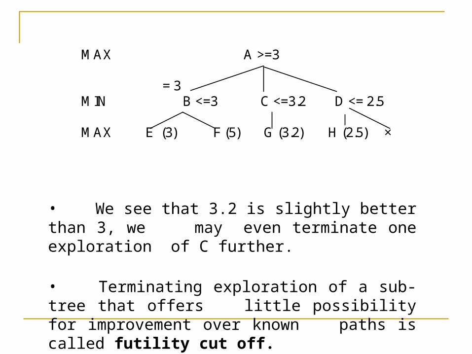
• We see that 3.2 is slightly better than 3, we may
even terminate one exploration of C further.
• Terminating exploration of a sub-tree that offers little possibility for improvement over known paths is called futility cut off.
MAX A >=3 = 3
MIN B <=3 C <=3.2 D <= 2.5
MAX E (3) F (5) G (3.2) H (2.5) ×
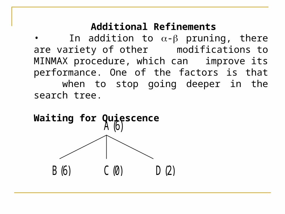
Additional Refinements• In addition to - pruning, there are variety of other
modifications to MINMAX procedure, which can improve its performance. One of the factors is that when to stop going deeper in the search tree.
Waiting for Quiescence
A (6)
B (6) C (0) D (2)
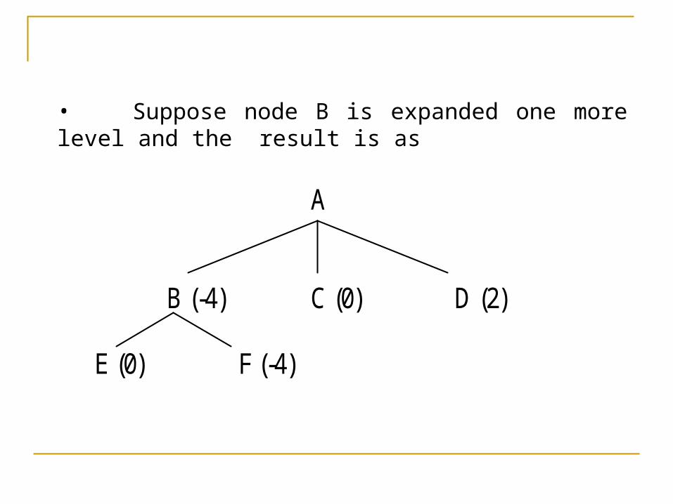
• Suppose node B is expanded one more level and the result is as
A
B (-4) C (0) D (2)
E (0) F (-4)
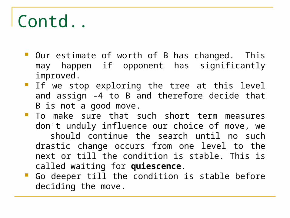
Contd..
Our estimate of worth of B has changed. This may happen if opponent has significantly improved.
If we stop exploring the tree at this level and assign -4 to B and therefore decide that B is not a good move.
To make sure that such short term measures don't unduly influence our choice of move, we should continue the search until no such drastic change occurs from one level to the next or till the condition is stable. This is called waiting for quiescence.
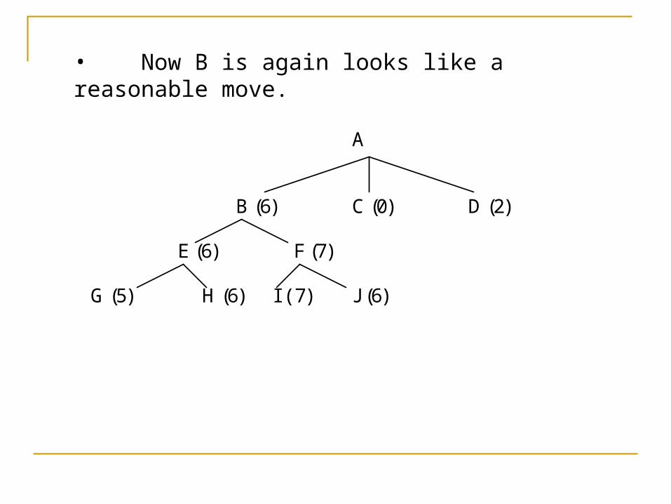
Go deeper till the condition is stable before deciding the move.
A
B (6) C (0) D (2)
E (6) F (7)
G (5) H (6) I ( 7) J (6)
• Now B is again looks like a reasonable move.
Secondary search• To provide a double check, explore a game tree to an
average depth of more ply and on the basis of that, chose a particular move. • Here chosen branch is further expanded up to two levels to make sure that it still looks good.• This technique is called secondary search.
Alternative to MINMAX• Even with refinements, MINMAX still has some problematic aspects. • It relies heavily on the assumption that the opponent
will always choose an optimal move.
Contd.. This assumption is acceptable in winning situations. But in losing situation it might be better to take risk that
opponent will make a mistake. Suppose we have to choose one move between two moves,
both of which if opponent plays perfectly, lead to situation that are very bad for us but one is slightly less bad than other.
Further less promising move could lead to a very good situation for us if the opponent makes a single mistake.
MINMAX would always choose the bad move. We instead choose the other one.
Similar situation occurs when one move appears to be only slightly more advantageous then another.
It might be better to choose less advantageous move. To implement such system we should have model of
individual opponents playing style.
Iterative Deepening Rather than searching to a fixed depth in the game tree, first
search only single ply, then apply MINMAX to 2 ply, further 3 ply till the final goal state is searched [CHESS 5 is based on this].
There is a good reason why iterative deepening is popular for chess-playing. In competition play there is an average amount of time allowed per move.
The idea that capitalizes on this constraint is to do as much look-ahead as can be done in the available time. If we use iterative deepening, we can keep on increasing the look-ahead depth until we run out of time.
We can arrange to have a record of the best move for a given look-ahead even if we have to interrupt our attempt to go one level deeper.


