PROBLEM SOLVINGTHROUGH FIRST-ORDER

LOGIC

by

Hashim Habiballa

Supervisor: Doc. RNDr. Alena Lukasová, CSc.

A thesis elaborated in partial fulfilment of the requirements for thedegree ofMagistr

in the Information Systems courseat

Department of Computer ScienceFaculty of Science

University of Ostrava,Ostrava, The Czech Republic.

April 1999

University of Ostrava

ii

Title: Problem solving through first-order logic.Author: Hashim Habiballa

Supervisor: Doc. RNDr. Alena Lukasová, CSc.Department: Computer Science

Degree: Mgr.Academic Year: 1998-99

Havířov, 13.4.1999

Permission is herewith granted to University of Ostrava to use and to have copied thepaper as well as to anyone interested in it. The same rights are given to the softwaretools accompanying the thesis.

The author attests that the thesis was disposed by his own effort and every source ofinformation used thereinafter was clearly acknowledged.

_____________________________Signature of Author

iii

PROBLEM SOLVING THROUGH FIRST-

ORDER LOGIC.

Theory and practice of non-clausal resolution.

Hashim HabiballaDepartment of Computer Science

Faculty of ScienceUniversity of Ostrava

Bráfova 7Ostrava 1

The Czech Republic.xhabibal@prf1.osu.cz

Abstract:

This thesis shows capabilities of non-clausal resolution on general formulas of first–order logic. The non-clausal resolution is presented both theoretically and practically bydesigning algorithms and programming the application for non-clausal inference. Theapplication should be treated like an experimental tool and should not be used for serioustheorem proving process. The paper will focus on the explanation of the algorithms andexamples showing their usage. It extends common notions of general resolution andresolution strategies.

iv

CZECH SUMMARY – SHRNUTÍ V ČEŠTINĚ

ŘEŠENÍ ÚLOH LOGIKOU PRVNÍHO ŘÁDU.

Teorie a praxe neklauzulární rezoluce.

Logika prvního řádu je dobře známá mezi matematiky a informatiky. Je to vhodnáformální reprezentace znalostí a teorémů. Ačkoliv je to populární a přímá cesta, problémautomatizovaného dokazování vět není až tak jednoduchý. Jestliže chcete využít sílulogiky, je nutné provést velké množství úprav, než je možné aplikovat deduktivnísystém. Tyto úpravy ničí význam formulí a mohou produkovat vysoký počet klauzulí (vpřípadě klauzulární rezoluce). Ovšem tyto systémy mají významné výhody jako jerychlost důkazu. Nicméně věřím, že z teoretického hlediska je velmi zajímavé pátrat podeduktivním systému, který nevyžaduje destruktivní transformace formulí.

Logika prvního řádu pokrývá mnoho deduktivních systémů. Přes vysokou rozmanitosttěchto systémů, mají jednu hlavní slabinu. Jsou určeny pouze pro omezenou tříduformulí. Byl jsem zklamán touto nevýhodou a hledal jsem nějaké řešení tohotoproblému. Na Internetu se nachází hodně spisů týkajících se rezoluce a mezi těmito spisyjsem nalezl článek "A theory of resolution" [Ba97], který představuje podrobný výčetmožností, jak provést rezoluci na skolemizovaných formulích. Tento článek jsem použilhlavně jako zdroj inspirace pro další výzkum strategií pro potlačení explozivního nárůstumnožství rezolvent a rozšíření teorie pro existenciální proměnné.

Neoddělitelnou částí této práce je počítačová aplikace, který má ilustrovat představenérezoluční techniky. Tato aplikace není odvozovacím systémem v plném slova smyslu,ale spíše má podepírat teoreticky dosažené výsledky. Doufám, že to je spolu sezmíněnými teoretickými rozšířeními malý příspěvek ke znalostem v automatizovanémdokazování vět.

Druhá kapitola definuje některé obecné pojmy. Kapitola tři zavádí obecnou rezoluci ademonstruje její použití na příkladech a také obsahuje některé modifikace a rozšířenívylepšující standardní definice, jak převzaté, tak originální. Kapitola čtyři uvádí doproblému vysokého počtu generovaných rezolvent a navrhuje možná řešenímodifikovaná či vytvořená pro účely této práce. Pátá kapitola popisuje algoritmy adatové struktury použité při vytváření aplikace. Pro tyto účely se užívá jazyka Pascal.Jelikož zdrojové kódy přesahují 100 KB, jsou představeny pouze naprosto zásadní části.Následující kapitola dává stručný přehled o možnostech aplikace nazvané GeneralizedResolution Deductive System (GERDS). Kapitola sedm přinese několik příkladů obecnérezoluce, což je pravděpodobně nejvhodnější cesta k porozumění metodám a síle obecnérezoluce.

v

Hlavní zamýšlený přínos práce je rozšířit a objasnit dříve objevená zevšeobecněnírezoluce. Měla by přinést zcela obecný deduktivní systém, který dokáže pracovats obecnými formulemi predikátové logiky, k čemuž potřebuje pouze charakteristikuextended polarity, která nevyžaduje žádné transformace formulí, ale pouze výpočetněkterých vlastností pro každou podformuli. Takový výpočet může být proveden běhemkonstrukce syntaktického stromu. Jestliže navíc nepožadujeme existenciální proměnné,pak je rezoluce zcela jednoduchá a nevyžaduje ani to.

Rozhodl jsem se psát práci v angličtině, neboť doufám že to dělá tuto práci vícesrozumitelnou a přístupnou širšímu okruhu čtenářů a proto je také prostá zbytečnýchdlouhých vysvětlování a raději se zaměřuje na příklady.

vi

ACKNOWLEDGEMENTS

There are many people, who had a significant effect to my private and professionallife during the pursuit of my study and the thesis. It‘s my best pleasure to express mythanks to everybody, who have had any influence to me.

I would like to start out by thanking my advisor Doc. RNDr. Alena Lukasová, CSc.,associate professor of logic on University of Ostrava. She evoked my interest inproblems of logic and artificial intelligence. I can‘t overlook our disputes on first-orderlogic, which was important source of inspiration for the objective of my research. Ofcourse, I have to consider the whole staff of the Department of Computer Science, whichcreates pleasant environment for study and work. I strongly appreciated computerequipment of the department, while I was working on the bachelor thesis two years ago.

During working on this project, I had an opportunity to utilize my own equipment. Itwas only possible, because my loving family, especially my mom Jana and grandmaMargareta, established for me the best home, I could imagine. I want to mention myArab relatives, especially my dad Salih for his support of me. I have had two goodfriends Radim and Viktor within the study and they helped me with the project. I amreally grateful for their sense of humour.

vii

CONTENTS

1 INTRODUCTION. ...............................................................................................................................1

2 PRELIMINARIES................................................................................................................................3

2.1 FIRST-ORDER LOGIC...........................................................................................................................3

2.2 REWRITE SYSTEMS..............................................................................................................................5

2.3 DEDUCTIVE SYSTEMS AND PRINCIPLES...............................................................................................6

3 GENERAL RESOLUTION.................................................................................................................8

3.1 DEFINITIONS AND EXAMPLES..............................................................................................................8

3.2 MODIFICATIONS................................................................................................................................10

3.3 POLARITY-BASED RESTRICTIONS.....................................................................................................12

3.4 EXTENDED POLARITY. ......................................................................................................................14

3.5 SIMPLIFICATION. ...............................................................................................................................15

3.6 LIFTING OF INFERENCES. ..................................................................................................................16

4 RESOLUTION STRATEGIES.........................................................................................................19

4.1 REFUTATION. ....................................................................................................................................19

4.2 STATE SPACE SEARCH. .....................................................................................................................19

4.3 COMMON STRATEGIES. .....................................................................................................................21

4.4 CHECK OF CONSEQUENCE. ................................................................................................................22

5 ALGORITHMS AND PROGRAMMING INTERFACE.............................................................24

5.1 PROGRAMMING TOOLS......................................................................................................................24

5.2 DATA STRUCTURES. ..........................................................................................................................24

5.3 PARSER. ............................................................................................................................................26

5.4 POSTPROCESSING..............................................................................................................................29

5.5 THEOREM PROVING...........................................................................................................................32

5.6 UNIFICATION.....................................................................................................................................35

5.7 SIMPLIFICATION AND CHECK OF CONSEQUENCE. .............................................................................36

6 COMPUTER APPLICATION. ........................................................................................................38

6.1 GENERAL INFORMATION...................................................................................................................38

6.2 INPUT AND OUTPUT. .........................................................................................................................39

6.3 PROOF. ..............................................................................................................................................40

viii

7 EXAMPLES. .......................................................................................................................................42

8 CONCLUSIONS. ................................................................................................................................49

9 REFERENCES....................................................................................................................................50

1

C h a p t e r 1

1 Introduction.

The first-order theory is well known among mathematicians and computer scientists.It is a suitable formal representation for expressing knowledge and theorems. Although itis very popular and clear way, the problem of automated theorem proving is not sosimple. If you want to enjoy the power of logic, you have to perform manytransformations, before you can use any deductive system. These transformationsdestroy the meaning of the formula and may produce high amount of clauses (in case ofclausal resolution). Of course, it has decisive advantages such as the efficiency of theproof. Nevertheless, I believe from the theoretical point of view it is a very interestinginvestigation to search for a deductive system, which is free of the need of destructivetransformations.

First-order logic covers many deductive systems. In spite of high diversity of thesesystems, they have one essential fault. They are determined to narrow class of formulas.I was disappointed from this fault and I looked for some solution to this problem. Therewas a lot of papers on the Internet concerning to resolution and among these papers Ifound a technical report ”A theory of resolution” [Ba97], which presents detailedexploration of the possibilities, how to perform deduction on skolemized formulas ofpredicate logic. Though the paper describes far more than the base extension ofresolution rule, I used the paper mainly as a source of inspiration for further research ofstrategies for suppressing the redundancy of an inference and handling existentialvariables.

The inseparable part of this thesis is the computer application, which has to illustratepresented resolution techniques. This application is not a full coverage of theoreticallyproposed deductive system. It doesn’t perform exact unification of existential variables;it handles only one-level existential formulas. I hope that it is together with thementioned theoretical extensions a small contribution to the knowledge in automatedtheorem proving.

The second chapter introduces some common notions (first-order logic, rewritesystems, deductive systems). Chapter three defines general resolution and brings someexamples, it also contains some modifications and extensions improving standarddefinitions both undertaken and self-devised. Chapter four shows the problem of highamount of resolvents generated during inference process and gives some commonsolutions and consequence checking specially modified for the purposes of this thesis.The fifth chapter describes application data structures and algorithms used for inferenceprocess in detail. It uses the Pascal programming language to demonstrate algorithmicalsolutions and Pascal comments to make the source code clearer. Since the source codeexceeds 100 KB, the chapter is as short as possible. The sixth chapter produces thedescription of the computer application called GEneralized Resolution Deductive

2

System (GERDS). GERDS supports my research in resolution techniques and it is notuser application in the right meaning. Of course one can use it, but must be aware ofbulks it contains. The sufficient and brief guide to the GERDS is given in this section.The section seven will show some examples of general resolution, which is probably themost suitable way to understand methods and power of general resolution.

The main intended contribution of the paper is to extend and illustrate previouslyfounded generalizations of deduction. It should bring the fully general deductive system,which may process general formulas of predicate logic and the only actual need is thenotion of extended polarity, which do not require any transformation, but only countingof some characteristics of every subformula. Such a counting can be performed duringthe construction of the parse tree, that is the most suitable representation for computerprocessing anyway. If we consider only non-existential formulas, then the resolution iscompletely trivial and does not require anything special.

I decided to write the thesis in English, since I hope that it makes the paper moreunderstandable and therefore there is as few useless words as possible.

3

C h a p t e r 2

2 Preliminaries.

2.1 First-Order Logic.

Before we start with the explanation of the general resolution, it is necessary tointroduce some common notations from first-order theory. It will be used the notationclose to logic programming. At first, it has to be shown the alphabet of the first-orderlogic language. Brief and pregnant explanation can be found in [Kl67] , [Ri89] or[No90]. It consists of:- Variables: Character string starting with a capital letter or underscore; containing

alphanumeric character or underscore, e.g. My_First_Var, _trash1.- Functors and predicates: Character string starting with a lower case letter e.g. sqrt,

is_a_Child. It is not actually needed to use a separate notion of the constant, becausethey can be treated as functions without arguments.

- Logical connectives: ý - conjunction, ü - disjunction, ô - implication, ó -equivalence, ¬ - negation.

- Logical constants: ç - false, ä - true. It is not used any special symbols in the sourceset for logical constants in the application, but there is a flag indicating logical valueof the subformula in the result and it is represented by ç and ä too.

- Quantifiers: ÷ - universal and ö - existential.- Special symbols: (, ) , and Ý, ß, <, >, =, á. The comparing characters have no

special handlers and serve as predicates for user usage.The best way to define the language of the First-order logic is the introduction of the

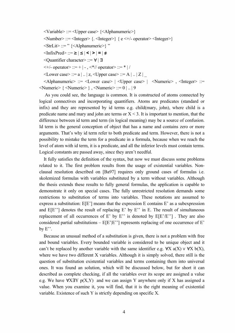
grammar in Backus –Naur Form:<Formula> ::= <Imp> { ó <Imp> }<Imp> ::= <Dis> { ô <Dis> }<Dis> ::= <Con> { ü <Con> }<Con> ::= <Subformula> { ý <Subformula> }<Subformula> ::= ¬ <Subformula> | <Quantifier section> <Subformula> | <Id Term>

| ‘[‘ <Formula> ‘]’ | <Atom> | <Id Term> <InfixPred> <Id Term><Quantifier section> ::= <Quantifier character> <Variable> { , <Variable> }

{<Quantifier character> <Variable> { , <Variable> } }<Id Term> ::= <Id Term2> { <+/- operator> <Id Term2> }<Id Term2> ::= <Id Base> { <*// operator> <Id Term2> }<Id Base> ::= <Variable> | <Functor> | <StrLit> | <Number> | + <Number> | -

<Number> | ( <Id Term> )<Functor> ::= <Lower case> {<Alphanumeric>} { ( <Id Term> { , <Id Term> } ) }

4

<Variable> ::= <Upper case> {<Alphanumeric>}<Number> ::= <Integer> {. <Integer>} { e <+/- operator> <Integer>}<StrLit> ::= ” {<Alphanumeric>} ”<InfixPred> ::= Ý | ß | < | > | = | á<Quantifier character> ::= ÷ | ö<+/- operator> ::= + | - , <*// operator> ::= * | /<Lower case> ::= a | .. | z, <Upper case> ::= A | .. | Z | _<Alphanumeric> ::= <Lower case> | <Upper case> | <Numeric> , <Integer> ::=

<Numeric> { <Numeric> } , <Numeric> ::= 0 | .. | 9 As you could see, the language is common. It is constructed of atoms connected by

logical connectives and incorporating quantifiers. Atoms are predicates (standard orinfix) and they are represented by id terms e.g. child(mary, john), where child is apredicate name and mary and john are terms or X < 3. It is important to mention, that thedifference between id term and term (in logical meaning) may be a source of confusion.Id term is the general conception of object that has a name and contains zero or morearguments. That’s why id term refer to both predicate and term. However, there is not apossibility to mistake the term for a predicate in a formula, because when we reach thelevel of atom with id term, it is a predicate, and all the inferior levels must contain terms.Logical constants are passed away, since they aren’t needful.

It fully satisfies the definition of the syntax, but now we must discuss some problemsrelated to it. The first problem results from the usage of existential variables. Non-clausal resolution described on [Ba97] requires only ground cases of formulas i.e.skolemized formulas with variables substituted by a term without variables. Althoughthe thesis extends these results to fully general formulas, the application is capable todemonstrate it only on special cases. The fully unrestricted resolution demands somerestrictions to substitution of terms into variables. These notations are assumed toexpress a substitution: E[E’] means that the expression E contains E’ as a subexpressionand E[E’’] denotes the result of replacing E’ by E’’ in E. The result of simultaneousreplacement of all occurrences of E’ by E’’ is denoted by E[E’/E’’] . They are alsoconsidered partial substitutions – E[E’|E’’] represents replacing of one occurrence of E’by E’’.

Because an unusual method of a substitution is given, there is not a problem with freeand bound variables. Every bounded variable is considered to be unique object and itcan’t be replaced by another variable with the same identifier e.g. ÷X a(X) ü ÷X b(X),where we have two different X variables. Although it is simply solved, there still is thequestion of substitution existential variables and terms containing them into universalones. It was found an solution, which will be discussed below, but for short it candescribed as complete checking, if all the variables over its scope are assigned a valuee.g. We have ÷XöY p(X,Y) and we can assign Y anywhere only if X has assigned avalue. When you examine it, you will find, that it is the right meaning of existentialvariable. Existence of such Y is strictly depending on specific X.

5

However, the main aspect of this thesis is lying on the resolution strategy, so one canomit the problem of existence and localize to formulas with indiscriminated variables.

Now we briefly summarize the semantics of first-order logic. First it is introduced thenotion of Interpretation.

Interpretation M = <D, f1, .., fn, p1, .., pn>, where D is a non-empty set called universe,fx represents functions, used in formulas, of the form f : Dp ô D and px representsrelations of predicates p ⊆ Dp . Further it is defined mapping e as variables evaluationfrom the set of all variables into D. Value of term t in M with evaluation e – t[e] is:

1. if t is variable X, then t[e] = e(X)2. if the term is of the form f(t1,..,tn), then t[e] = fI(t1[e],..,tn[e])We define, that the formula F is true in M with evaluation e - M é F[e] as follows:

1. if F is a predicate of the form p(t1,..,tn), then M é F[e] iff (t1,..,tn) ∈ pM, pM isappropriate relation from M.

2. if F is of the form ¬G then, M é F[e] iff M é G[e] doesn‘t hold.3. if F is one of the form G ý H, G ü H, G ô H, G ó H, then M é F[e] depending on

the connective iff M é G[e] and M é H[e], iff M é G[e] or M é H[e], and so on for other connectives.

4. if F is of the form ÷X G, where G is a formula of the language, then M é F[e] iff forevery case m ∈ D : M é G[e[x/m]].

5. if F is of the form öX G, where G is a formula of the language, then M é F[e] iffthere is a case m ∈ D : M é G[e[x/m]].

Formula F is satisfiable in M, if for some e M é F[e] holds. F is satisfied (valid) in M -M é F, if M é F[e] for every e. If the formula is satisfied in every interpretation, then itis (logically) true.

2.2 Rewrite systems.

Next, the notion of rewrite systems is revised, which are well known for example fromthe theory of formal languages. They will be used to describe rewriting of formulas insimplification methods. It is defined Eσ, which represents applying the substitution σ toformula E and it is called an instance of E. Eσ without variables is called groundinstance.

A rewrite system is a binary relation on formulas with metavariables, the elements,which are called rewrite rules and written F ⇒ F’. Metavariables represents formulasand that’s why complex formulas can be rewritten in the same way as atoms.(Occasionally it is possible to consider two way rewrite rule F ⇔ F’, if a rewrite systemcontains both F ⇒ F’ and F’ ⇒ F.) We denote by ⇒R the smallest rewrite relation thatcontains all instances Fσ ⇒ F’σ of rule in R. F can be rewritten to F’ by R, if F ⇒R F’.

Here are some examples. Consider R containing De Morgan’s rules:¬( A ý B) ⇒ (¬A ü ¬B) , ¬( A ü B) ⇒ (¬A ý ¬B) and ¬¬A ⇒ A .

6

Such a system allows us to rewrite every formula, containing only conjunctions,disjunctions and negations, to the form, in which negation is put down to atoms.

For example:¬ (a ý ¬(b ü c) ) ü ¬d ⇒ ( ¬ a ü ¬¬(b ü c)) ü ¬d ⇒ ( ¬ a ü (b ü c)) ü ¬dSo we can write that ¬ (a ý ¬(b ü c) ) ü ¬d ⇒R ( ¬ a ü (b ü c)) ü ¬dOf course, it is only simplified definition, but there is no need to extend it.

2.3 Deductive systems and principles.

Let’s have a look to two deductive systems of first-order logic to see the advantagesand disadvantages of them. A detailed description of these systems can be found in[Lu95] or [Ce81]. Deductive (Axiomatic) system consists of :1. Language.2. Axioms – source formulas (schemas) for inferring theorems.3. Rules - enabling to derive theorems from axioms.

Since it is a basic subject matter, it will not be described exact grammar of a system.And by reason that we are interested in theorem proving from the set of special axioms,we stay on discussing about the construction of formulas and inference rules.

First let’s stop with the Hilbert’s axiomatic system.It has two allowed connectives – negation and implication. Although it is known that

negation and implication forms complete set of connectives i.e. every formula can berewritten to it, the lucidity of the proof is low. We can dispute about some special casessuch as Horn clauses: a1 ý .. ý an ô b. They are simply and clearly transformable into a1

ô( ..ô (an ô b)), but some simple cases with equivalence or negation in superior levelslike ¬(a ü b) (⇒ ¬(¬a ô b)) have the meaning of the formula hardly recognizable. Thefirst transformation is quite close to Hilbert style: ” if a1 holds and .. and an holds thenb holds too” transforms to ”if a1 holds then if .. then if an hold then b holds too. Thesecond one is recondite ”it doesn’t hold a or b” (in the other words a doesn’t hold and bdoesn’t hold) transforms to ” it doesn’t hold that if a doesn’t hold then b holds”. Please,try to think about it and if the Hilbert representation seems clear to you, you have naturalturn in logic.

In the other hand the modus ponens rule looks smart, as we can understand it : ”ifholds the theorem of the form - if a then b and if a holds, then b must hold too.” Theaxiom of specification ensures the possibility of transformations of formulas into theirground cases.

The second deductive system uses the best known principle, it is the resolutiondeductive system with the resolution principle. Language of the system acceptsformulas in conjunctive normal form. The resolution rule is notoriously known:

Consider two clauses of the form C1 ü l and C2 ü l’, where l and l’ are mutuallycomplementary. Then it can be deduced from the two above clauses the clause C1 ü C2 .This type of a rule also has a reasonable sense. Let’s take the modus ponens rule and try

7

to see it as a specialization of the resolution rule. A ô B could be rewritten to ¬A ü Band that’s why the MP rule has the resolution form: ¬A ü B and A faces to B. Theresolution rule can be also considered in the implicative form and then it can viewed astransitive rule A ü B , ¬B ü C ⇒ ¬A ô B , B ô C, which gives ¬A ô C that is A ü C. Sothe complementary couple of atoms is redundant and can be omitted, if we construct newimplicative theorem. It consents to the clausal meaning. The two complementary atomsin the conjunction have no gain, because there is no model depending only on these twoliterals. So that’s why every model of ( C1 ü l ) ý ( C2 ü l’ ) on C1 or C2 only. In theother words ( C1 ü l ) and ( C2 ü l’ ) must be both true in such model, but then C1 mustbe true if l is false or C2 must be true if l is true and no other case exists. This is a littleless clear explanation than an implicative form, I’m convinced.

When we considered these two systems, we didn’t speak about predicate logicmodifications of these systems deeply. It was a wilful omission. These extended versionsdo not require a lot of effort to devise. It is the question of finding the right way to makeformulas ground and to handle existence. The first one is solved with unifiers (inresolution based systems) or rules of specialization (in Hilbert system) and the secondone is solved by skolemization (transformation of existential variable to a new functionwith superior variables as arguments) or implicitly by special functors (in Clausal FormLogic).

8

C h a p t e r 3

3 General Resolution.

3.1 Definitions and examples.

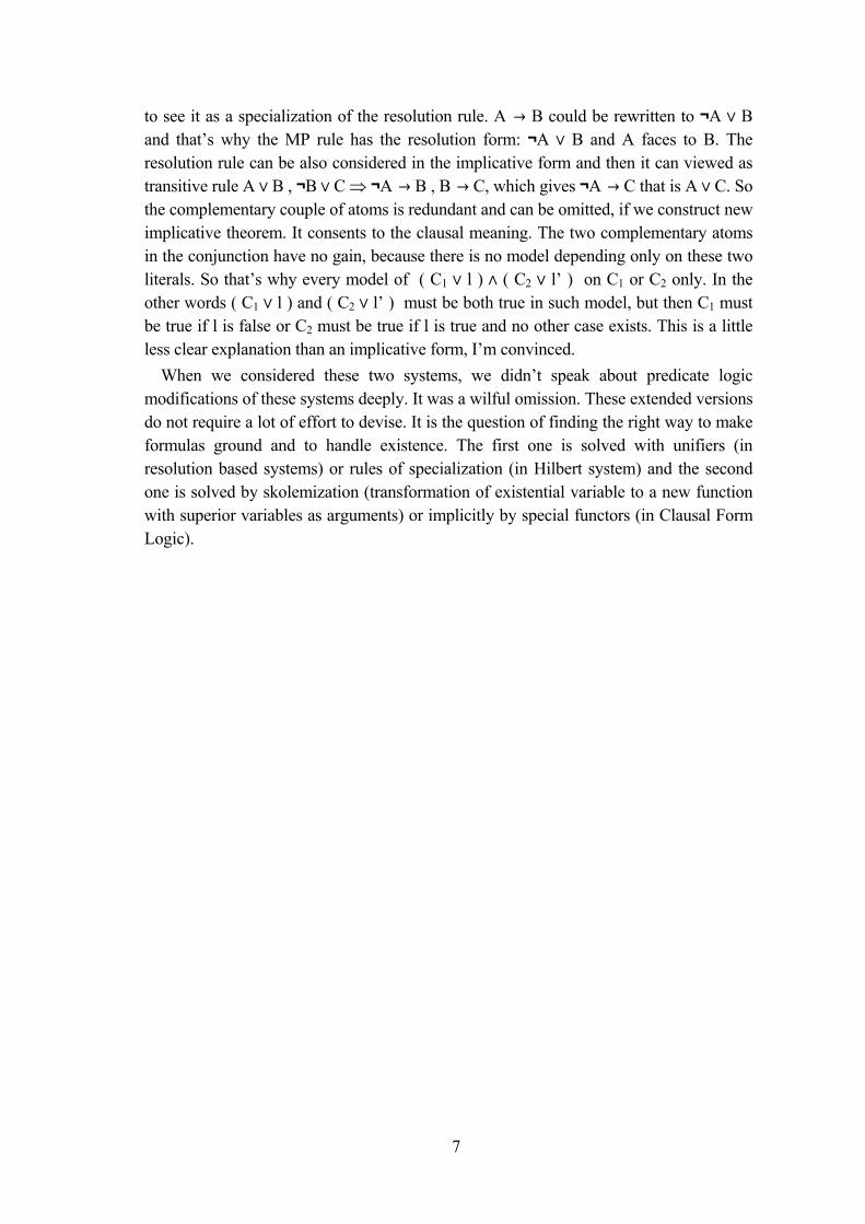
When we use refutational theorem proving, we deduce new formulas from given onesand negated goal and search for a contradiction. The widely used inference rule isresolution, originally introduced by Robinson. Now we present the results from [Ba97]to show the power of general resolution that applies to general formulas. Becausehereinbefore we discussed that it is possible to stay on propositional case and then onlyfind suitable unification method to extend it, let’s start with propositional forms of rulesas presented in [Ba97].

For the purposes of mentioned article, there were introduced some notions. Inferencerule is an n-ary relation on expressions, where n Ý 1. The elements of such relation arewritten as

E1 .. En-1————

E

and called inferences. The expressions E1 .. En-1 are called premises, and E is theconclusion, of the inference. An inference system is a collection of inference rules.

An inference is sound if the conclusion is a logical consequence of the premises, i.e.,E1 .. En-1 é E . The following definition of resolution for formulas is sound.

Definition 0.1: General resolution.

F[G] F‘[G]—————————F[G / ç] ü F’[G / ä]

It is the resolution on G and the conclusion of the inference is called resolvent of thetwo premises. It is also called F the positive, F’ the negative premise, and G the resolvedsubformula. As you see, the rule is highly general, since it allows resolving on wholesubformulas. Nevertheless, it will be used only resolution on atomic subformulas in thisthesis. The proof of the soundness of the rule is similar to clausal resolution rule proof.Suppose the Interpretation I in which both premises are valid. In I, G is either true orfalse. If G (¬G) is true in I, so is F[G / ä] (F[G / ç ]). From this point of view, it shows,that the resolution rule is nothing more that assertion of the type: If we have twoformulas holding simultaneously and they contain the same formula, then we can deducethat either the common subformula is true in this interpretation then the truthfulness is

9

assured by the first formula or the second formula in the opposite case. Now we canhave a look to the question, how these facts influence the view of clausal resolution.

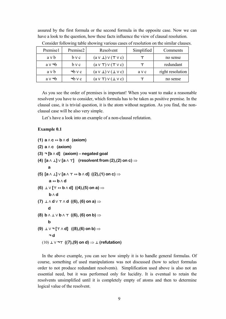
Consider following table showing various cases of resolution on the similar clauses.Premise1 Premise2 Resolvent Simplified Comments

a ü b b ü c (a ü ç) ü (ä ü c) ä no sensea ü ¬b b ü c (a ü ä) ü (ä ü c) ä redundanta ü b ¬b ü c (a ü ç) ü (ç ü c) a ü c right resolution

a ü ¬b ¬b ü c (a ü ä) ü (ç ü c) ä no sense

As you see the order of premises is important! When you want to make a reasonableresolvent you have to consider, which formula has to be taken as positive premise. In theclausal case, it is trivial question, it is the atom without negation. As you find, the non-clausal case will be also very simple.

Let’s have a look into an example of a non-clausal refutation.

Example 0.1

(1) a ý c ó b ý d (axiom)

(2) a ý c (axiom)

(3) ¬ [b ý d] (axiom) – negated goal

(4) [a ý ç] ü [a ý ä] (resolvent from (2),(2) on c) ⇒

a

(5) [a ý ç] ü [a ý ä ó b ý d] ((2),(1) on c) ⇒

a ó b ý d

(6) ç ü [ä ó b ý d] ((4),(5) on a) ⇒

b ý d

(7) ç ý d ü ä ý d ((6), (6) on a) ⇒

d

(8) b ý ç ü b ý ä ((6), (6) on b) ⇒

b

(9) ç ü ¬ [ä ý d] ((8),(6) on b) ⇒

¬ d

(10) ç ü ¬ä ((7),(9) on d) ⇒ ç (refutation)

In the above example, you can see how simply it is to handle general formulas. Ofcourse, something of used manipulations was not discussed (how to select formulasorder to not produce redundant resolvents). Simplification used above is also not anessential need, but it was performed only for lucidity. It is eventual to retain theresolvents unsimplified until it is completely empty of atoms and then to determinelogical value of the resolvent.

10

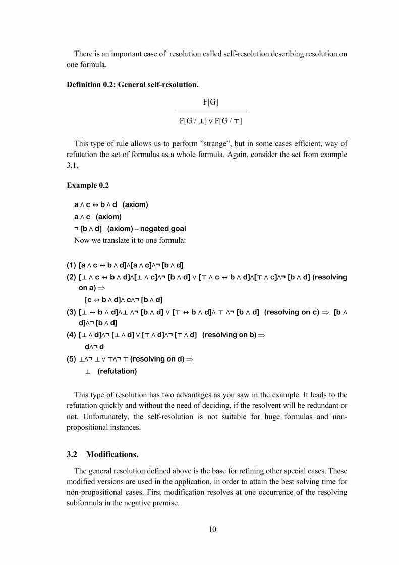
There is an important case of resolution called self-resolution describing resolution onone formula.

Definition 0.2: General self-resolution.

F[G]—————————

F[G / ç] ü F[G / ä]

This type of rule allows us to perform ”strange”, but in some cases efficient, way ofrefutation the set of formulas as a whole formula. Again, consider the set from example3.1.

Example 0.2

a ý c ó b ý d (axiom)

a ý c (axiom)

¬ [b ý d] (axiom) – negated goal

Now we translate it to one formula:

(1) [a ý c ó b ý d]ý[a ý c]ý¬ [b ý d]

(2) [ç ý c ó b ý d]ý[ç ý c]ý¬ [b ý d] ü [ä ý c ó b ý d]ý[ä ý c]ý¬ [b ý d] (resolving

on a) ⇒

[c ó b ý d]ý cý¬ [b ý d]

(3) [ç ó b ý d]ýç ý¬ [b ý d] ü [ä ó b ý d]ý ä ý¬ [b ý d] (resolving on c) ⇒ [b ý

d]ý¬ [b ý d]

(4) [ç ý d]ý¬ [ç ý d] ü [ä ý d]ý¬ [ä ý d] (resolving on b) ⇒

dý¬ d

(5) çý¬ ç ü äý¬ ä (resolving on d) ⇒

ç (refutation)

This type of resolution has two advantages as you saw in the example. It leads to therefutation quickly and without the need of deciding, if the resolvent will be redundant ornot. Unfortunately, the self-resolution is not suitable for huge formulas and non-propositional instances.

3.2 Modifications.

The general resolution defined above is the base for refining other special cases. Thesemodified versions are used in the application, in order to attain the best solving time fornon-propositional cases. First modification resolves at one occurrence of the resolvingsubformula in the negative premise.

11

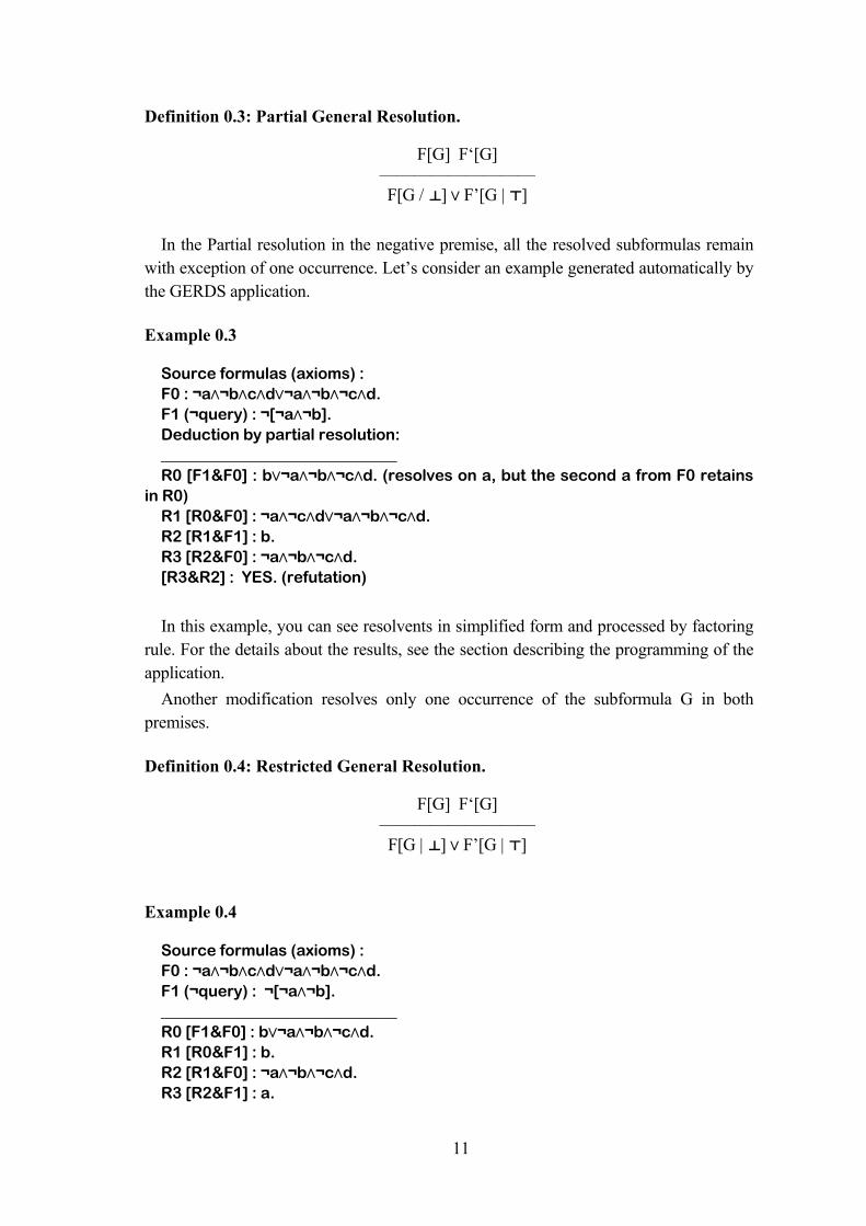
Definition 0.3: Partial General Resolution.

F[G] F‘[G]—————————F[G / ç] ü F’[G | ä]

In the Partial resolution in the negative premise, all the resolved subformulas remainwith exception of one occurrence. Let’s consider an example generated automatically bythe GERDS application.

Example 0.3

Source formulas (axioms) :F0 : ¬aý¬býcýdü¬aý¬bý¬cýd.F1 (¬query) : ¬[¬aý¬b].Deduction by partial resolution:______________________________R0 [F1&F0] : bü¬aý¬bý¬cýd. (resolves on a, but the second a from F0 retains

in R0)R1 [R0&F0] : ¬aý¬cýdü¬aý¬bý¬cýd.R2 [R1&F1] : b.R3 [R2&F0] : ¬aý¬bý¬cýd.[R3&R2] : YES. (refutation)

In this example, you can see resolvents in simplified form and processed by factoringrule. For the details about the results, see the section describing the programming of theapplication.

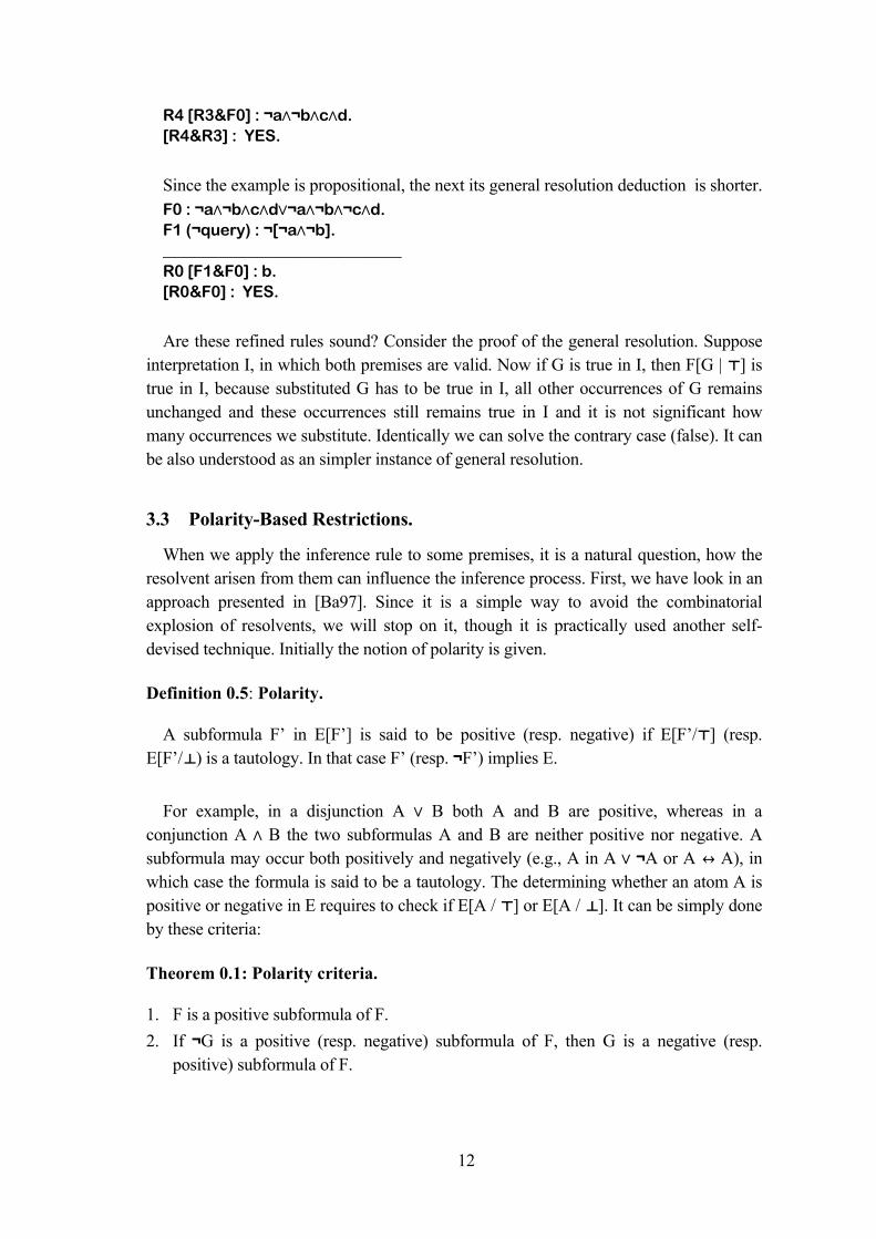
Another modification resolves only one occurrence of the subformula G in bothpremises.

Definition 0.4: Restricted General Resolution.

F[G] F‘[G]—————————F[G | ç] ü F’[G | ä]

Example 0.4

Source formulas (axioms) :F0 : ¬aý¬býcýdü¬aý¬bý¬cýd.F1 (¬query) : ¬[¬aý¬b].______________________________R0 [F1&F0] : bü¬aý¬bý¬cýd.R1 [R0&F1] : b.R2 [R1&F0] : ¬aý¬bý¬cýd.R3 [R2&F1] : a.

12

R4 [R3&F0] : ¬aý¬býcýd.[R4&R3] : YES.

Since the example is propositional, the next its general resolution deduction is shorter.F0 : ¬aý¬býcýdü¬aý¬bý¬cýd.F1 (¬query) : ¬[¬aý¬b].______________________________R0 [F1&F0] : b.[R0&F0] : YES.

Are these refined rules sound? Consider the proof of the general resolution. Supposeinterpretation I, in which both premises are valid. Now if G is true in I, then F[G | ä] istrue in I, because substituted G has to be true in I, all other occurrences of G remainsunchanged and these occurrences still remains true in I and it is not significant howmany occurrences we substitute. Identically we can solve the contrary case (false). It canbe also understood as an simpler instance of general resolution.

3.3 Polarity-Based Restrictions.

When we apply the inference rule to some premises, it is a natural question, how theresolvent arisen from them can influence the inference process. First, we have look in anapproach presented in [Ba97]. Since it is a simple way to avoid the combinatorialexplosion of resolvents, we will stop on it, though it is practically used another self-devised technique. Initially the notion of polarity is given.

Definition 0.5: Polarity.

A subformula F’ in E[F’] is said to be positive (resp. negative) if E[F’/ä] (resp.E[F’/ç) is a tautology. In that case F’ (resp. ¬F’) implies E.

For example, in a disjunction A ü B both A and B are positive, whereas in aconjunction A ý B the two subformulas A and B are neither positive nor negative. Asubformula may occur both positively and negatively (e.g., A in A ü ¬A or A ó A), inwhich case the formula is said to be a tautology. The determining whether an atom A ispositive or negative in E requires to check if E[A / ä] or E[A / ç]. It can be simply doneby these criteria:

Theorem 0.1: Polarity criteria.

1. F is a positive subformula of F.2. If ¬G is a positive (resp. negative) subformula of F, then G is a negative (resp.

positive) subformula of F.

13

3. If G ü H is a positive subformula of F, then G and H are both positive subformulas ofF.

4. If G ý H is a negative subformula of F, then G and H are both negative subformulasof F.

5. If G ô H is a positive subformula of F, then G is a negative subformula and H is apositive subformula of F.

6. If G ô ç is a negative subformula of F, then G is a positive subformula of F.

The proof of the theorem is trivial and it is established on the notoriously known senseof logical connectives. Now it is possible to state two restrictions based on above.

Theorem 0.2: Redundancy of general resolution.

An inference by general resolution is redundant if the negative premise contains apositive occurrence of the resolved atom or if the positive premise contains a negativeoccurrence of the resolved atom.

Proof: If the negative premise contains a positive occurrence of the resolved atom A,then the resolvent appears as follows: F[A / ç] ü F’[A / ä] ⇒ F[A / ç] ü ä ⇒ ä. If thepositive premise contains a negative occurrence of the resolved atom A, then theresolvent appears as follows: F[A / ç] ü F’[A / ä] ⇒ ä ü F’[A / ç] ⇒ ä. In both theseinstances resolvents degenerate to tautologies. In the refutational proof, such cases areimproductive, i.e. from these resolvents can’t be deduced false.

Theorem 0.3: Redundancy of general self-resolution.

An inference by general self-resolution is redundant if the resolved atom occurspositively or negatively in the premise.

Proof: If the premise contains a positive occurrence of the resolved atom A, then theresolvent appears as follows: F[A / ç] ü F[A / ä] ⇒ F[A / ç] ü ä ⇒ ä. If the premisecontains a negative occurrence of the resolved atom A, then the resolvent appears asfollows: F[A / ç] ü F[A / ä] ⇒ ä ü F[A / ç] ⇒ ä. In both these instances resolventsdegenerate to tautologies. In the refutational proof, such cases are improductive, i.e.from these resolvents can’t be deduced false.

Example 0.5

Let’s consider two premises:1. ¬A – A is negative.2. A ý B – A is neither positive nor negative.

The resolvent of 1. and 2. is ¬ç ü [ä ý B] ⇒ ä.

14

3.4 Extended Polarity.

As it was noticed above, it is important to decide which of the two premises to betaken as positive. It has been developed a simple way to decide it during making of thisthesis. It is an extended notion of polarity, which is similar to definition of Murray(1982), but the usage is different here.

Definition 0.6: Extended Polarity.

The subformula F is said to be positive (resp. negative) in E if after the transformationof E to conjunction-normal form, where F is treated as an atom, F would not be negated(would be negated).

It is clear, that every subformula has some polarity and if some of its superiorconnectives is equivalence, then it is both positive and negative. Following theoremgives algorithm for determination of polarity.

Theorem 0.4: Extended Polarity criteria.

1. F is a positive subformula of F.2. If ¬G is a positive (resp. negative) subformula of F, then G is a negative (resp.

positive) subformula of F.3. If G ü H is a positive (resp. negative) subformula of F, then G and H are both

positive (resp. negative) subformulas of F.4. If G ý H is a positive (resp. negative) subformula of F, then G and H are both

positive (resp. negative) subformulas of F.5. If G ô H is a positive (resp. negative) subformula of F, then G is a negative (resp.

positive) subformula and H is a positive (resp. negative) subformula of F.6. If G ó H is a subformula of F, then every subformula of G and H is positive and

negative subformula of F.

Then it is possible to set the formula with positive polarity as the positive premise.This solves the problem of wrong order of premises i.e. it avoids redundant resolvents.

Example 0.6

Source formulas (axioms) :F0 : aüb.F1 : ¬büc.F2 (¬query) : ¬[aüc].______________________________R0 [F2&F2] : ¬c.R1 [F2&F1] : ¬b.

15

R2 [F2&F0] : b.R3 [F1&F2] : ¬b.R4 [F1&F0] : cüa. ( c as negative premise)R5 [F0&F2] : b.R6 [F0&F1] : aüc. ( a as positive premise)[R5&R3] : YES.

R4 was created as resolvent of F1 and F0 where F1 was treated as a negative premise:(¬ä ü c) ü (a ü ç).

3.5 Simplification.

In the above subsections, it was applied the obvious notion of simplification forformulas. Although it is the clear process, the rewrite rules, which are the sources for thesimplification, are stated here.

At the beginning, we mention the rules for eliminating logical constants fromconjunctions, disjunctions and negations:

A ý ç ⇒ ç ç ý A ⇒ çA ý ä ⇒ A ä ý A ⇒ AA ü ç ⇒ A ç ü A ⇒ AA ü ä ⇒ ä ä ü A ⇒ ä

¬ç ⇒ ä ¬ä ⇒ ç

For other connectives, there are similar rules:A ô ç ⇒ ¬A ç ô A ⇒ äA ô ä ⇒ ä ä ô A ⇒ A

A ó ç ⇒ ¬A ç ó A ⇒ ¬AA ó ä ⇒ A ä ó A ⇒ A

Another important rule reducing the length of a formula is the factoring rule. Theclausal form of the rule could be presented as follows:

a1 ü .. ü an ü a ü a—————————

a1 ü .. ü an ü awhere ax and a are arbitrary atoms and the order of the atoms is insignificant.This rule can be used also in the general case (general formulas) as a partial

simplification technique.

16

3.6 Lifting of Inferences.

The general resolution presented was based on the propositional calculus. The liftingof resolution inferences to formulas with indiscriminated variables into universal andexistential ones follows below. For instance, general resolution.

F[G] F‘[G]—————————F[G / ç] ü F’[G / ä]

is lifted toF[G1,...,Gk] F‘[G’1,...,G’n]

————————————Fσ[G / ç] ü F’σ[G / ä]

where σ is the most general unifier (mgu) of the atoms G1,...,Gk , G’1,...,G’n , G = G1σ,and in contrast with [Ba97] it is not supposed renaming of the variables for the purposesof the application. We can suppose, that every variable occurring in a quantifier has itsown identifier (for example address), which is assigned to variable occurrence).Technical details can be found in the section describing the programming of theapplication.

For the second open problem it has been devised the extension of mgu. Basically, itfunctions as follows:

Definition 0.7: Most general unifier.

1. When both the terms to unify are of the type string, number or functor withoutparameters then they are unifiable iff its type is the same (e.g. string and string andso on) and their identifiers match.

2. When one of the terms is a variable then it is unifiable with the second one iffVariable Unification Restriction holds.

3. If both the terms are of the type functor with arguments, then they are unifiable iffall the arguments are unifiable by the same procedure from the point 1. ( The orderof unification to be mentioned with respect to unification of variables, so it tries tounify the atom until it expands the mgu from the first ununified term.)

4. There is no other possibility to unify two terms, except that two object of unificationare the same physically (e.g. During the a self-resolution the occurrence of twovariables points to the same variable).

The following discrimination of existential and universal variables is needed for theVariable Unification Restriction definition:

When we speak about existential and universal variables, it is related to its notion withrespect to the scope of the whole formula e.g. In öX÷Y p(X,Y) ô a(Z) Y variable to betreated as an existential variable, because the p(X,Y) subformula has negative extendedpolarity. It means, if we translate the formula into clausal form, Y would transform intoexistential variable. We define the discrimination as follows.

17

The discrimination of variables:Variable quantified by existential (resp. universal) quantifier is said to be globally

existential (resp. globally universal), if the extended polarity of the subformula, whichowns the quantifier (the quantifier prefixes it), is positive and it is said to be globallyuniversal (resp. globally existential), if the the extended polarity is negative. If thepolarity is both negative and positive, the variable is both globally existential anduniversal.

Variable Unification Restriction holds if one of the conditions 1. and 2. is satisfied:1. One of the terms is a globally universal variable and the second one does not contain

a globally existential variable. (non-existential case)2. One of the terms is a globally universal variable, the second one contains a globally

existential variable, and every variable over the scope of the existential one hasassigned any value.

Remark: The above definition determines, that two globally existential variables can’t beunified, that is clear.

Let’s have a look in an example of well-known facts:It doesn’t hold ÷XöY p(X, Y) é öY÷X p(X,Y) andit holds öY÷X p(X, Y) é ÷XöY p(X,Y).

( General Y for all X can’t be deduced from Y specific for X but contrary it holds. )

Example 0.7

Source formulas (axioms) :F0 : ÷XöY p(X, Y).F1 (¬query) : ÷YöX ¬p(X, Y).______________________________[F1&F1] : çü ä.[F0&F0] : çü ä.

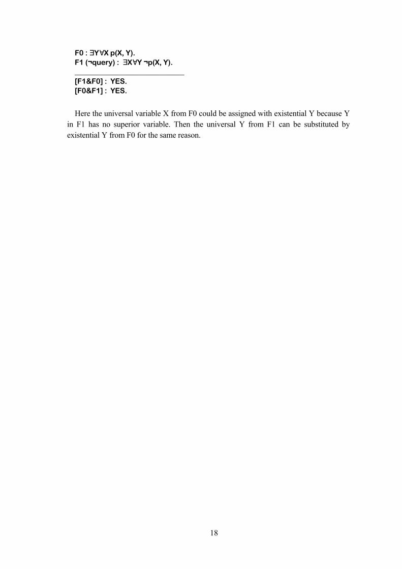
In this sample F0 and F1 can’t resolve, since ÷XöY p(X, Y) and ÷YöX ¬p(X, Y) haveno unifier. It is impossible to substitute universal X from F0 with X from F1, because Xfrom F1 is existential and its superior variable Y is not assigned with a value. Counter-example with variable Y is the same instance and it is not allowed to substitute anythinginto an existential variable.

However, in the next example an unifier exists.

Example 0.8

Source formulas (axioms) :

18

F0 : öY÷X p(X, Y).F1 (¬query) : öX÷Y ¬p(X, Y).______________________________[F1&F0] : YES.[F0&F1] : YES.

Here the universal variable X from F0 could be assigned with existential Y because Yin F1 has no superior variable. Then the universal Y from F1 can be substituted byexistential Y from F0 for the same reason.

19

C h a p t e r 4

4 Resolution strategies.

4.1 Refutation.

As it has been written, the theorem proving method, which is used, is calledrefutational proof. Firstly the goal is negated, it is added to the set of axioms and thenone searches for false formula using inference rules. Completeness of the refutationalresolution proof is almost done by the proof for clausal instance presented in [Lu95]. Itonly should be replaced the conception of clauses by general formulas and consider theproof of soundness of the general resolution rule.

In next sections, several types of resolution strategies are presented, which may avoidgenerating huge amount of resolvents. In the beginning breadth-first and depth-firstsearch are recalled, then important characteristics of linear search, filtration strategy andsupport-set strategy are summarized, in the end it is presented self-devised algorithm toreduce redundancy. Very good source of information about these strategies can be foundin [Ma93].

4.2 State Space Search.

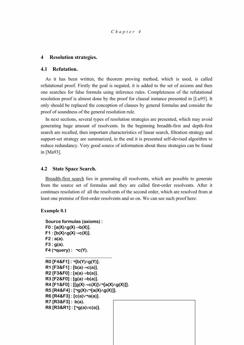
Breadth-first search lies in generating all resolvents, which are possible to generatefrom the source set of formulas and they are called first-order resolvents. After itcontinues resolution of all the resolvents of the second order, which are resolved from atleast one premise of first-order resolvents and so on. We can see such proof here:

Example 0.1

Source formulas (axioms) :F0 : [a(X)ýg(X)ôb(X)].F1 : [b(X)ýg(X)ôc(X)].F2 : a(a).F3 : g(a).F4 (¬query) : ¬c(Y).______________________________R0 [F4&F1] : ¬[b(Y)ýg(Y)].R1 [F3&F1] : [b(a)ôc(a)].R2 [F3&F0] : [a(a)ôb(a)].R3 [F2&F0] : [g(a)ôb(a)].R4 [F1&F0] : [[g(X)ôc(X)]ü¬[a(X)ýg(X)]].R5 [R4&F4] : [¬g(X)ü¬[a(X)ýg(X)]].R6 [R4&F3] : [c(a)ü¬a(a)].R7 [R3&F3] : b(a).R8 [R3&R1] : [¬g(a)üc(a)].

20

R9 [R1&F4] : ¬b(a).R10 [R1&R7] : c(a).R11 [R0&R7] : ¬g(a).[R11&F3] : YES.Y = a.[R10&F4] : YES.Y = a.[R9&R7] : YES.Y = a.R12 [R9&R2] : ¬a(a).[R7&R9] : YES.Y = a.[R12&F2] : YES.Y = a.

Figure 4.1. shows how the resolvents were obtained. You can see that there are fourlevels of resolvents.

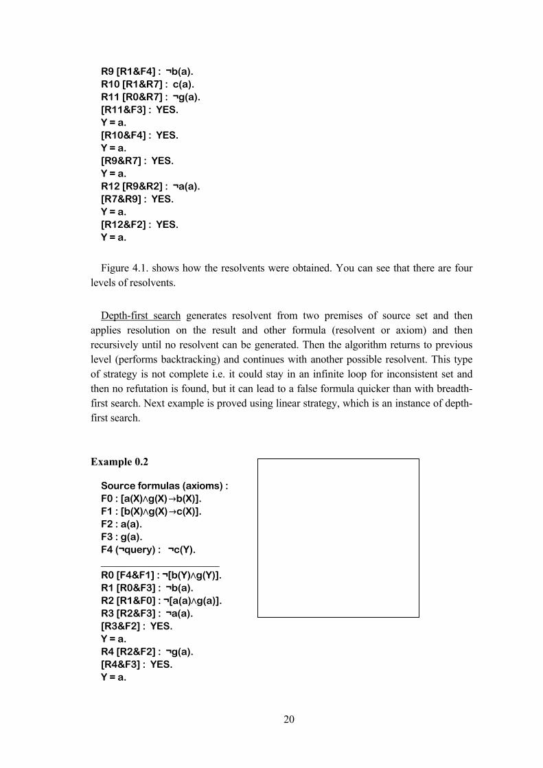
Depth-first search generates resolvent from two premises of source set and thenapplies resolution on the result and other formula (resolvent or axiom) and thenrecursively until no resolvent can be generated. Then the algorithm returns to previouslevel (performs backtracking) and continues with another possible resolvent. This typeof strategy is not complete i.e. it could stay in an infinite loop for inconsistent set andthen no refutation is found, but it can lead to a false formula quicker than with breadth-first search. Next example is proved using linear strategy, which is an instance of depth-first search.

Example 0.2

Source formulas (axioms) :F0 : [a(X)ýg(X)ôb(X)].F1 : [b(X)ýg(X)ôc(X)].F2 : a(a).F3 : g(a).F4 (¬query) : ¬c(Y).________________________R0 [F4&F1] : ¬[b(Y)ýg(Y)].R1 [R0&F3] : ¬b(a).R2 [R1&F0] : ¬[a(a)ýg(a)].R3 [R2&F3] : ¬a(a).[R3&F2] : YES.Y = a.R4 [R2&F2] : ¬g(a).[R4&F3] : YES.Y = a.

21

Figure 4.2. illustrate the simplicity of linear proof in comparison to previous example.

4.3 Common strategies.

Common strategies to reduce the set of resolvents include the wide-used Linearstrategy. Example 4.2 was produced using this type of strategy. Linear strategy utilizeslast generated clause as one of the premises. Linear strategies preserve the sequence of aproof. It is a base technique for logic programming. Other strategies are primarilyintended for breadth-first search, but can be also invoked in depth-first search. Alreadymentioned disadvantage implies from its incompleteness. In the application, we use twodifferent notions of linear search – linear, which generates resolvents only from goal andmodified linear search, which is not restricted only to goal.

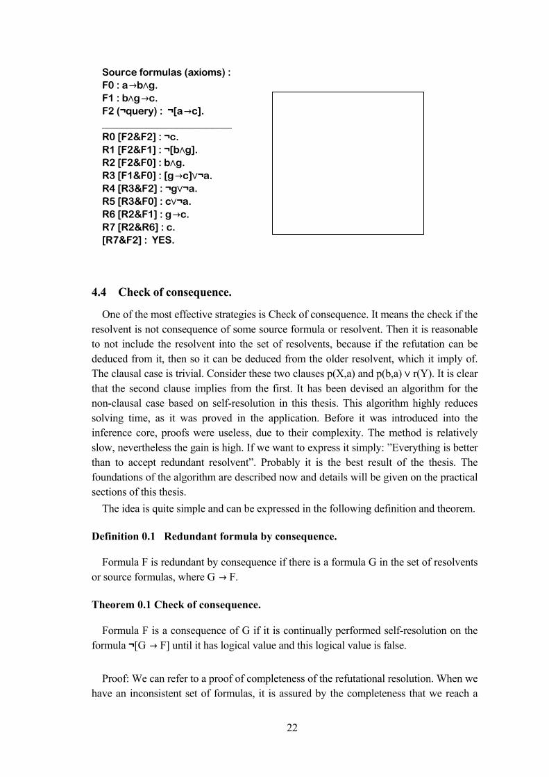
The Support Set Strategy is simple, but also incomplete strategy. It rises from the factthat there is an consistent subset in every source set of formulas. It is obvious that theresolvents from this subset can’t lead to false formula. That’s why this strategy allows toresolve such premises, from which one is the goal or its descendant. Let’s again have alook in an example for the same set of formulas as above.

Example 0.3

R0 [F4&F1] : ¬[b(Y)ýg(Y)].R1 [R0&F3] : ¬b(a).R2 [R0&F0] : [¬g(Y)ü¬[a(Y)ýg(Y)]].R3 [R2&F3] : ¬a(a).R4 [R2&F2] : ¬g(a).[R4&F3] : YES.Y = a.[R3&F2] : YES.Y = a.

Support set strategy in this example is far more efficient than the unoptimized search.

The filtration strategy is the next resolvent reducing method. Two premises A,B canbe resolved only if one of these conditions holds:1. A or B is from the source set of formulas2. A is a descendant of B or B is descendant of A.

( Descendant notion refers to the resolution tree.)It is complete strategy, although it is not so efficient as last strategy.

Example 0.4

With filtration:

22

Source formulas (axioms) :F0 : aôbýg.F1 : býgôc.F2 (¬query) : ¬[aôc].__________________________R0 [F2&F2] : ¬c.R1 [F2&F1] : ¬[býg].R2 [F2&F0] : býg.R3 [F1&F0] : [gôc]ü¬a.R4 [R3&F2] : ¬gü¬a.R5 [R3&F0] : cü¬a.R6 [R2&F1] : gôc.R7 [R2&R6] : c.[R7&F2] : YES.

4.4 Check of consequence.

One of the most effective strategies is Check of consequence. It means the check if theresolvent is not consequence of some source formula or resolvent. Then it is reasonableto not include the resolvent into the set of resolvents, because if the refutation can bededuced from it, then so it can be deduced from the older resolvent, which it imply of.The clausal case is trivial. Consider these two clauses p(X,a) and p(b,a) ü r(Y). It is clearthat the second clause implies from the first. It has been devised an algorithm for thenon-clausal case based on self-resolution in this thesis. This algorithm highly reducessolving time, as it was proved in the application. Before it was introduced into theinference core, proofs were useless, due to their complexity. The method is relativelyslow, nevertheless the gain is high. If we want to express it simply: ”Everything is betterthan to accept redundant resolvent”. Probably it is the best result of the thesis. Thefoundations of the algorithm are described now and details will be given on the practicalsections of this thesis.

The idea is quite simple and can be expressed in the following definition and theorem.

Definition 0.1 Redundant formula by consequence.

Formula F is redundant by consequence if there is a formula G in the set of resolventsor source formulas, where G ô F.

Theorem 0.1 Check of consequence.

Formula F is a consequence of G if it is continually performed self-resolution on theformula ¬[G ô F] until it has logical value and this logical value is false.

Proof: We can refer to a proof of completeness of the refutational resolution. When wehave an inconsistent set of formulas, it is assured by the completeness that we reach a

23

false formula . And since one formula forms a set and the self-resolution is a special caseof general resolution, we can say that if ¬[G ô F] is inconsistent then we prove it byself-resolution i.e. we prove that G ô F is a tautology.

Example 0.5

Consider the formula [a ü b] ý [¬b ü c] and we prove that [a ü c] is a consequence ofit.(1) ¬[[aüb]ý[¬büc]ôaüc]

(2) ¬[[ çüb]ý[¬büc]ô çüb]ü¬[[ äüb]ý[¬büc]ô äüb] ⇒ ç

It was used the factoring rule for the simplification on the line (2).

24

C h a p t e r 5

5 Algorithms and programming interface.

5.1 Programming tools.

It was exploited excellent development environment for the production of theapplication performing theoretically presented manipulations in the previous chapters.The Borland Delphi 2 with the Object Pascal language is thought as this tool offeringmany objective extensions to standard Pascal. This language is utilized to present thealgorithms for the inference techniques. It is supposed that the reader has an essentialknowledge of Pascal. First we start with the data structures, the construction of parsetrees and then we focus to resolution methods. To get an introduction to Pascal languagesee [Ji88] or electronic help of Delphi 2. There is a very good source of informationabout data structures such as stack in [Be71].

5.2 Data structures.

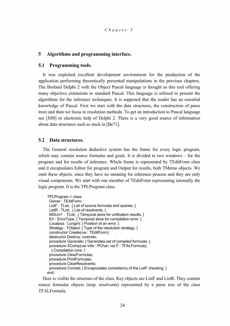
The General resolution deductive system has the frame for every logic program,which may contain source formulas and goals. It is divided to two windows – for theprogram and for results of inference. Whole frame is represented by TEditForm classand it encapsulates Editor for program and Output for results, both TMemo objects. Weomit these objects, since they have no meaning for inference process and they are onlyvisual components. We start with one member of TEditForm representing internally thelogic program. It is the TPLProgram class.

TPLProgram = class Owner : TEditForm; ListF : TList; { List of source formulas and queries. } ListR : TList; { List of resolvents. } MGUn1 : TList; { Temporal store for unification results. } Err : ErrorType; { Temporal store for compilation error. } Localpos : Longint; { Position of an error. } Strategy : TObject; { Type of the resolution strategy. } constructor Create(ow : TEditForm); destructor Destroy; override; procedure Generate; { Generates set of compiled formulas. } procedure XComp(var infix : PChar; var F : TFALFormula); { Compilation core. } procedure ClearFormulas; procedure PrintFormulas; procedure ClearResolvents; procedure Consist; { Encapsulates consistency of the ListF checking. }end;

Here is visible the structure of the class. Key objects are ListF and ListR. They containsource formulas objects (resp. resolvents) represented by a parse tree of the classTFALFormula.

25

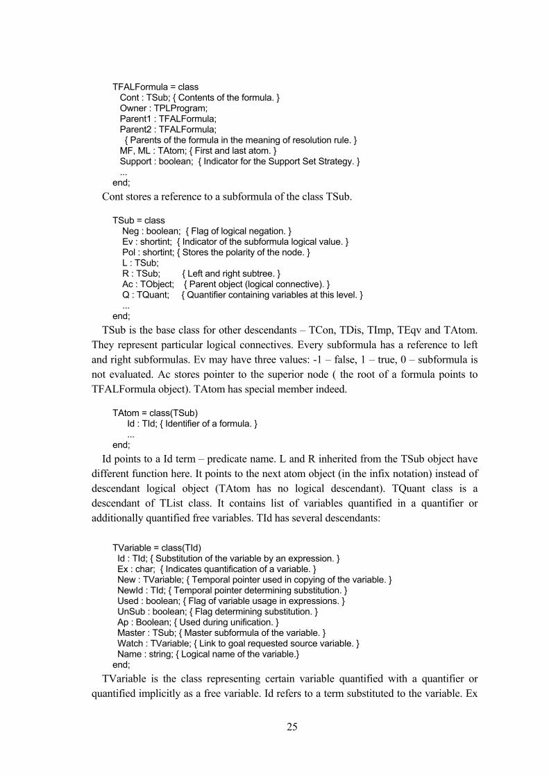
TFALFormula = class Cont : TSub; { Contents of the formula. } Owner : TPLProgram; Parent1 : TFALFormula; Parent2 : TFALFormula; { Parents of the formula in the meaning of resolution rule. } MF, ML : TAtom; { First and last atom. } Support : boolean; { Indicator for the Support Set Strategy. } ...end;

Cont stores a reference to a subformula of the class TSub.

TSub = class Neg : boolean; { Flag of logical negation. } Ev : shortint; { Indicator of the subformula logical value. } Pol : shortint; { Stores the polarity of the node. } L : TSub; R : TSub; { Left and right subtree. } Ac : TObject; { Parent object (logical connective). } Q : TQuant; { Quantifier containing variables at this level. } ...end;

TSub is the base class for other descendants – TCon, TDis, TImp, TEqv and TAtom.They represent particular logical connectives. Every subformula has a reference to leftand right subformulas. Ev may have three values: -1 – false, 1 – true, 0 – subformula isnot evaluated. Ac stores pointer to the superior node ( the root of a formula points toTFALFormula object). TAtom has special member indeed.

TAtom = class(TSub) Id : TId; { Identifier of a formula. } ...end;

Id points to a Id term – predicate name. L and R inherited from the TSub object havedifferent function here. It points to the next atom object (in the infix notation) instead ofdescendant logical object (TAtom has no logical descendant). TQuant class is adescendant of TList class. It contains list of variables quantified in a quantifier oradditionally quantified free variables. TId has several descendants:

TVariable = class(TId) Id : TId; { Substitution of the variable by an expression. } Ex : char; { Indicates quantification of a variable. } New : TVariable; { Temporal pointer used in copying of the variable. } NewId : TId; { Temporal pointer determining substitution. } Used : boolean; { Flag of variable usage in expressions. } UnSub : boolean; { Flag determining substitution. } Ap : Boolean; { Used during unification. } Master : TSub; { Master subformula of the variable. } Watch : TVariable; { Link to goal requested source variable. } Name : string; { Logical name of the variable.}end;

TVariable is the class representing certain variable quantified with a quantifier orquantified implicitly as a free variable. Id refers to a term substituted to the variable. Ex

26

may obtain two values: cforall – constant of universal quantifier character ÷ or cexists –existential character ö. New is used, when a new copy of a formula is created. It pointsto newly created variable. NewId points to a term, which has to be substituted and fromthis term is created a copy assigned later to New variable. Master refers to thesubformula, which quantifies the variable. Watch is the observing reference to thevariable from the goal of the logic program. It is created, in order to show the assignmentof variables, which led to a contradiction. After direct compilation, all occurrences of avariable in terms are not assigned to one object of the class TVariable, but to anotherdescendant of TId – TVar. TVar consist of Name only and serves as temporal class,before the TVariable is assigned to an occurrence.

Further TId descendants are: TStrLit, TReal, TInteger, TFunctor and TFunctora,which represent string, real number, integer, functor with arguments and functor withoutarguments.

Now let’s see into some illustrations of parse trees of formulas.Consider this simple formula:

Example 0.1

÷X p(X,30) ý öY r("string",Y) ô q(const,X).Direct compilation:

The example of the object hierarchy of the parse tree shows, how the variables areassigned to particular occurrences of them. After variable assignment there is a newquantifier, which quantifies former free variable X. It was created in the root of the tree,since free variables have global scope.

5.3 Parser.

Last subsection analyzed the data structures of formulas and indicated that the parsetree plays the main role in the practical use of general resolution. The editor of the logicprogram source is accessible as a null-terminated string and the main parsing procedureTPLProgram.XComp uses this string.

procedure TPLProgram.XComp; begin ... StackInit; cpos := 0; dontcare := 0;Error := OK;Getchar; if (ch = '?')and(infix[cpos] = '-') then begin query := true;GetCharI; GetChar; end; if Error = OK then Eqv; { Go to parser / generator. } ... if Error = endcomp then

27

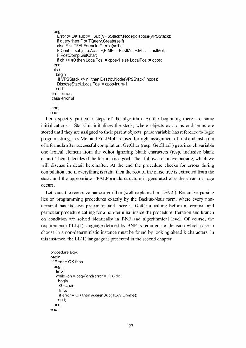
begin Error := OK;sub := TSub(VPSStack^.Node);dispose(VPSStack); if query then F := TQuery.Create(self) else F := TFALFormula.Create(self); F.Cont := sub;sub.Ac := F;F.MF := FirstMol;F.ML := LastMol; F.PostComp;GetChar; if ch <> #0 then LocalPos := cpos-1 else LocalPos := cpos; end else begin if VPSStack <> nil then DestroyNode(VPSStack^.node); DisposeStack;LocalPos := cpos-inum-1; end; err := error; case error of ... end;end;

Let’s specify particular steps of the algorithm. At the beginning there are someinitializations – StackInit initializes the stack, where objects as atoms and terms arestored until they are assigned to their parent objects, parse variable has reference to logicprogram string, LastMol and FirstMol are used for right assignment of first and last atomof a formula after successful compilation. GetChar (resp. GetCharI ) gets into ch variableone lexical element from the editor ignoring blank characters (resp. inclusive blankchars). Then it decides if the formula is a goal. Then follows recursive parsing, which wewill discuss in detail hereinafter. At the end the procedure checks for errors duringcompilation and if everything is right then the root of the parse tree is extracted from thestack and the appropriate TFALFormula structure is generated else the error messageoccurs.

Let’s see the recursive parse algorithm (well explained in [Dv92]). Recursive parsinglies on programming procedures exactly by the Backus-Naur form, where every non-terminal has its own procedure and there is GetChar calling before a terminal andparticular procedure calling for a non-terminal inside the procedure. Iteration and branchon condition are solved identically in BNF and algorithmical level. Of course, therequirement of LL(k) language defined by BNF is required i.e. decision which case tochoose in a non-deterministic instance must be found by looking ahead k characters. Inthis instance, the LL(1) language is presented in the second chapter.

procedure Eqv;begin if Error = OK then begin Imp; while (ch = ceqv)and(error = OK) do begin Getchar; Imp; if error = OK then AssignSub(TEqv.Create); end; end;end;

28

Here it is presented the procedure Eqv related to <Formula> non-terminal (expressesequivalence level with the lowest priority). It dives to Imp non-terminal procedure firstand then continues zero or more times with the same non-terminal depending if someequivalence character is found. Every such equivalence is created and it has assigned Land R descendant by AssignSub procedure by the following way.

procedure AssignSub(Ob : TObject); { Assigns formula its subtrees. }begin Put(Ob);pom := Cut; TSub(pom^.node).R := TSub(VPSStack^.node); TSub(VPSStack^.node).Ac := pom^.node; garbage := Cut;dispose(garbage); TSub(pom^.node).L := TSub(VPSStack^.node); TSub(VPSStack^.node).Ac := pom^.node; garbage := Cut;dispose(garbage);SInsert(pom);end;

Put procedure creates a stack object, which encapsulates every object’s life in thestack and enables the logical object to be bounded in the stack with the succeedingobject. Then it pops from stack with Cut procedure and it is stored in the pom variable. Itis assigned the first object in the stack into the R pointer of pom object. Then the same isdone with the second object. They are simultaneously removed from the stack since theyare now elements of the parse tree. Resulting object is then put in the stack and waitsuntil it is attached to its superior node.

The procedure ICE related to <Subformula> fully demonstrates the recursivecharacter of such algorithm.

procedure ICE;beginif error = OK then begin case ch of cneg : begin Getchar; ICE;NegateF; end; cforall, cexists : begin Quant; ICE; if Error = OK then AssignQtoSub; end; 'a'..'z', 'A'..'Z', '_', '0'..'9', '"', '(', '+', '-' : begin Atom; end; '[' : begin GetChar; Eqv; if (ch <> ']')and(error = OK) then Error := missbra; Getchar; end else if error = OK then Error := missexp; end; end;end;

29

The cneg case refers to a negated subformula and it recursively calls the sameprocedure. The second case of quantifiers does the similar work.

The third case handles an occurrence of atom and it remains to solve the case ofsubformula enclosed in brackets. It is obvious that the other parser procedures areomitted, because they use the same principle.

5.4 Postprocessing.

There is still something undone after successful compilation. It is inevitable to assignvariables instead of TVar objects for every occurrence of a variable, it is also needed toevaluate the extended polarity of nodes and it is useful to perform evaluation ofconstants connected by infix operators. These operations are encapsulated in the nextprocedure.

procedure TFALFormula.PostComp;var TT1 : TAtom;begin LastSub := nil; Dive('4', VarReAssign, [nil]); { Assignment of variables. } Dive('3', EvalBuilt, [nil]); { Evaluation of infix operators. } Cont.EvalPol;end;

Dive procedure has three arguments. It is the general procedure, which helps tobrowse parse tree without the need to write the same code for different actions. The firstargument determines the manner of browsing inside the tree e.g. ‘3’ – postorder (first goto subtrees and then performs a operation on the node, details in [Be71]). The secondargument sends a reference to the procedure, which does the actions. Last argument maysend some additional information in the form of variant array i.e. special item of ObjectPascal language, which allows to work with variable number of arguments ofchangeable types. The executive procedure (second par.) must have this form:

TDoProc = function(o : TObject; var tp : char; argums : array of const) : TObject; { Template for functions used as executive procedures for the recursive browsing of the syntactical tree.(ST) }

It accepts reference o to the current object, the currently valid mode of browsing andalready mentioned variant arguments and it returns reference to an object, which willreplace the assignment of the current node if the modification is needed.

Before we continue with the postprocessing, let’s have a look into an example of theimplementation of the Dive procedure:

function TSub.Dive;var i : longint;begin case tp of '1' : begin

30

Proc(self, tp, argums); if Q <> nil then Q.Dive(tp, proc, argums); if L <> nil then L.Dive(tp, proc, argums); if R <> nil then R.Dive(tp, proc, argums); end; ... 'r' : begin Result := TSub(ClassType.Create); Result.Neg := Neg; Result.Ev := Ev;Result.Pol := Pol; Result.Ac := Ancs; LastSub := Result; if Q <> nil then begin Result.Q := Q.Dive(tp, proc, argums); if Result.Q <> nil then with Result.Q do for i := 0 to Count-1 do TVariable(Items[i]).Master := Result; end; Ancs := Result; LastSub := Result; if L <> nil then Result.L := L.Dive(tp, proc, argums); Ancs := Result; LastSub := Result; if R <> nil then Result.R := R.Dive(tp, proc, argums); LastSub := Result; if Q <> nil then Q.Dive('q', proc, argums); end; ...end;

Of course, a lot of code was cut short, but there still remains illustrative sample. The‘1’ mode means preorder type of browsing i.e. First perform Proc (executive procedure)on the node and then go recursively into descendant trees. The ‘r’ mode expresses theaction of copying the tree and as you see, the result variable assures the right assignmentof new object members.

If we return to the beginning of this subsection, we can continue with explanation ofthe PostComp procedure.

{ Procedure for assignment of complex variable object for every occurrence of the variable. }function VarReAssign(o1 : TObject; var tp : char; argums : array of const) : TObject;var S1 : TSub; i : integer; O : TVariable;begin Result := o1; if o1 is TSub then ... else if (o1 is TVar) then begin S1 := LastSub; O := nil; if S1.Q <> nil then with S1.Q do begin for i := 0 to Count-1 do { Searches for right TVariable object. } if TVariable(Items[i]).Name = TVar(o1).Id then O:=TVariable(Items[i]); end; while not(S1.Ac is TFALFormula)and(O = nil) do

31

begin S1 := TSub(S1.Ac); if S1.Q <> nil then with S1.Q do begin for i := 0 to Count-1 do if TVariable(Items[i]).Name = TVar(o1).Id then O := TVariable(Items[i]); end; end; if O <> nil then begin o1.Free; end else begin if S1.Q = nil then S1.Q := TQuant.Create; O := TVariable.Create(TVar(o1)); O.Ap := false; O.Master := S1; { If not found, creates new variable on } o1.Free; { the top level. } O.Ex := cforall;S1.Q.Add(O); end; Result := O; end;end;

It is important factor, which subformula is the nearest superior node in this executiveprocedure. It can be found from the LastSub variable. From this points it starts to searchfor the nearest variable, which match the name of the occurrence. It continues to theparent node and tries to match the name, but if it doesn’t succeed until the root isreached, it creates a new variable and appends it into the root quantifier. It set up theMaster property of the variable, which points to the subformula, which includes thequantifier encapsulating the variable.

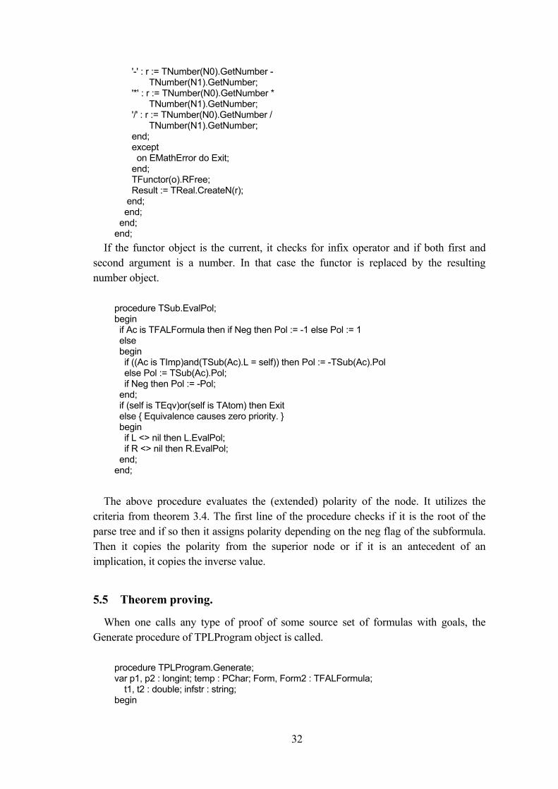
{ Evaluates infix operators. }function EvalBuilt(o : TObject; var tp : char; argums : array of const) : TObject;var r : extended; N0, N1 : TObject; fc : char;begin Result := o; if o is TFunctor then begin if (TFunctor(o).Functor[1] in infixoper) then begin N0 := (TFunctor(o).Params.Items[0]); N1 := (TFunctor(o).Params.Items[1]); while N0 is TVariable do N0 := TVariable(N0).Id; while N1 is TVariable do N1 := TVariable(N1).Id; if (N0 is TNumber)and(N1 is TNumber) then begin try case TFunctor(o).Functor[1] of '+' : r := TNumber(N0).GetNumber + TNumber(N1).GetNumber;

32

'-' : r := TNumber(N0).GetNumber - TNumber(N1).GetNumber; '*' : r := TNumber(N0).GetNumber * TNumber(N1).GetNumber; '/' : r := TNumber(N0).GetNumber / TNumber(N1).GetNumber; end; except on EMathError do Exit; end; TFunctor(o).RFree; Result := TReal.CreateN(r); end; end; end;end;

If the functor object is the current, it checks for infix operator and if both first andsecond argument is a number. In that case the functor is replaced by the resultingnumber object.

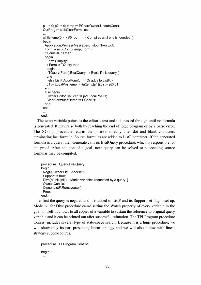
procedure TSub.EvalPol;begin if Ac is TFALFormula then if Neg then Pol := -1 else Pol := 1 else begin if ((Ac is TImp)and(TSub(Ac).L = self)) then Pol := -TSub(Ac).Pol else Pol := TSub(Ac).Pol; if Neg then Pol := -Pol; end; if (self is TEqv)or(self is TAtom) then Exit else { Equivalence causes zero priority. } begin if L <> nil then L.EvalPol; if R <> nil then R.EvalPol; end;end;

The above procedure evaluates the (extended) polarity of the node. It utilizes thecriteria from theorem 3.4. The first line of the procedure checks if it is the root of theparse tree and if so then it assigns polarity depending on the neg flag of the subformula.Then it copies the polarity from the superior node or if it is an antecedent of animplication, it copies the inverse value.

5.5 Theorem proving.

When one calls any type of proof of some source set of formulas with goals, theGenerate procedure of TPLProgram object is called.

procedure TPLProgram.Generate;var p1, p2 : longint; temp : PChar; Form, Form2 : TFALFormula; t1, t2 : double; infstr : string;begin

33

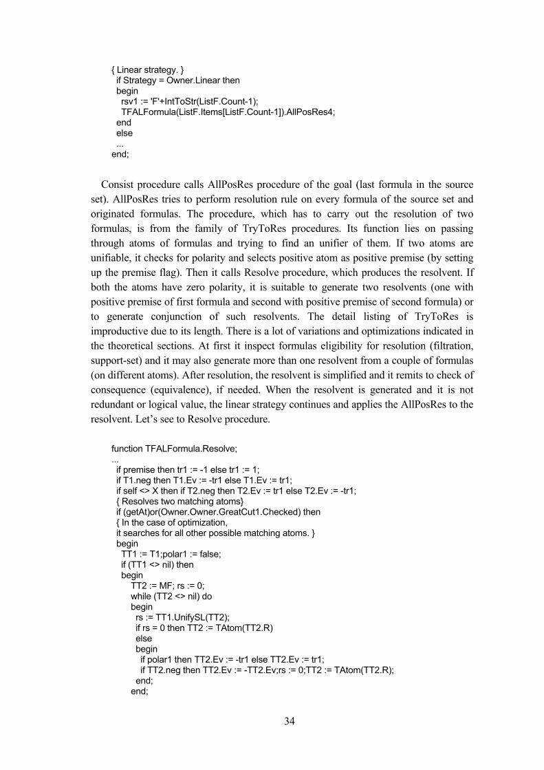
p1 := 0; p2 := 0; temp := PChar(Owner.UpdateCont); CurProg := self;ClearFormulas; ... while temp[0] <> #0 do { Compiles until end is founded. } begin Application.ProcessMessages;if stopf then Exit; Form := nil;XComp(temp, Form); if Form <> nil then begin Form.Simplify; if Form is TQuery then begin TQuery(Form).EvalQuery; { Evals if it is query. } end else ListF.Add(Form); { Or adds to ListF. } p1 := LocalPos;temp := @(temp[p1]);p2 := p2+p1; end else begin Owner.Editor.SelStart := p2+LocalPos+1; ClearFormulas; temp := PChar(''); end; end; ...end;

The temp variable points to the editor’s text and it is passed through until no formulais generated. It may raise both by reaching the end of logic program or by a parse error.The XComp procedure returns the position directly after dot and blank charactersterminating last formula. Source formulas are added to ListF container. If the generatedformula is a query, then Generate calls its EvalQuery procedure, which is responsible forthe proof. After solution of a goal, next query can be solved or succeeding sourceformulas may be compiled.

procedure TQuery.EvalQuery;begin NegQ;Owner.ListF.Add(self); Support := true; Dive('v', nil, [nil]); { Marks variables requested by a query. } Owner.Consist; Owner.ListF.Remove(self); Free;end;

At first the query is negated and it is added to ListF and its Support-set flag is set up.Mode ‘v’ for Dive procedure cause setting the Watch property of every variable in thegoal to itself. It allows to all copies of a variable to sustain the reference to original queryvariable and it can be printed out after successful refutation. The TPLProgram procedureConsist includes several type of state-space search. Because it is a huge procedure, wewill show only its part presenting linear strategy and we will also follow with linearstrategy subprocedures.

procedure TPLProgram.Consist;...begin ...

34

{ Linear strategy. } if Strategy = Owner.Linear then begin rsv1 := 'F'+IntToStr(ListF.Count-1); TFALFormula(ListF.Items[ListF.Count-1]).AllPosRes4; end else ...end;

Consist procedure calls AllPosRes procedure of the goal (last formula in the sourceset). AllPosRes tries to perform resolution rule on every formula of the source set andoriginated formulas. The procedure, which has to carry out the resolution of twoformulas, is from the family of TryToRes procedures. Its function lies on passingthrough atoms of formulas and trying to find an unifier of them. If two atoms areunifiable, it checks for polarity and selects positive atom as positive premise (by settingup the premise flag). Then it calls Resolve procedure, which produces the resolvent. Ifboth the atoms have zero polarity, it is suitable to generate two resolvents (one withpositive premise of first formula and second with positive premise of second formula) orto generate conjunction of such resolvents. The detail listing of TryToRes isimproductive due to its length. There is a lot of variations and optimizations indicated inthe theoretical sections. At first it inspect formulas eligibility for resolution (filtration,support-set) and it may also generate more than one resolvent from a couple of formulas(on different atoms). After resolution, the resolvent is simplified and it remits to check ofconsequence (equivalence), if needed. When the resolvent is generated and it is notredundant or logical value, the linear strategy continues and applies the AllPosRes to theresolvent. Let’s see to Resolve procedure.

function TFALFormula.Resolve;... if premise then tr1 := -1 else tr1 := 1; if T1.neg then T1.Ev := -tr1 else T1.Ev := tr1; if self <> X then if T2.neg then T2.Ev := tr1 else T2.Ev := -tr1; { Resolves two matching atoms} if (getAt)or(Owner.Owner.GreatCut1.Checked) then { In the case of optimization, it searches for all other possible matching atoms. } begin TT1 := T1;polar1 := false; if (TT1 <> nil) then begin TT2 := MF; rs := 0; while (TT2 <> nil) do begin rs := TT1.UnifySL(TT2); if rs = 0 then TT2 := TAtom(TT2.R) else begin if polar1 then TT2.Ev := -tr1 else TT2.Ev := tr1; if TT2.neg then TT2.Ev := -TT2.Ev;rs := 0;TT2 := TAtom(TT2.R); end; end;

35

end; if (self <> X)and ((getat)or(Owner.Owner.General.Checked)) then begin ... { Identical code, but for the second formula } end; end; PrepareMgu;FL.Cont := F3; F3.Ac := FL;Ancs := F3; TN2 := T2; F1 := Cont.Dive('r', nil, [nil]); { Makes a copy of the first formula with substituted variables. } Ancs := F3; TM1 := LastMol; TN2 := nil; if (self = X) then begin invert := true;F2 := X.Cont.Dive('r', nil, [nil]);invert := false; end else F2 := X.Cont.Dive('r', nil, [nil]); ...end;

First mentioned lines perform assignment of a logical value to resolved atoms. Itdepends on premise flag, which indicate that the first formula – self has to be treated asthe positive premise and the second formula X has to be regarded as the negativepremise. Of course, it is useless to evaluate the second atom, if self=X. Next it evaluatesall atoms from the positive premise, if the user requires it by checking off the Generalcut (Partial resolution) item from the application menu. If the general cut item is checkedoff, then all atoms from the second formula are evaluated and resolve procedure carrieson general resolution. Otherwise it evaluates only two atoms and this is animplementation of restricted resolution. PrepareMgu assigns unifier substitution from thetemporal TList store named mgu1 into the appropriate variable NewId property. Thennew disjunction is created and copies of premises made by ‘r’ mode of the Diveprocedure are assigned as L and R references to this disjunction. There is also specialprocedure for self-resolution called ResolveAWC.

5.6 Unification.

The key factor of lifting inferences to non-ground cases of formulas is the mostgeneral unifier. The function responsible for unification is TAtom.UnifyS andTAtom.UnifyId is its executive procedure, which unifies Id properties of two atoms.

function TId.UnifyId;var varn : integer;begin varn := mgu1.Count-1; repeat unres1 := 1; { Tries to unify id terms until, it is clear that } unres := 1; { no more changes are done. } varn := mgu1.count; Dive('5', IdUnif, [X]); if unres1 = 0 then unres := 0; until (varn = mgu1.count)or(unres <> 0);end;

36

The ground or non-existential instance is trivial and one pass is enough, but in theexistential case the order of arguments in functors is important. That’s why it tries tounify two terms until any substitution is not realized or the unification is completelyimpossible. What it means? The unres variable is set to zero, if two constant objectscan’t be unified, while unres1 is set zero even if some variable can’t be unified. So if avariable was taken in a wrong order, we can still remain it ununified and wait for thenext pass, which will occur only if some other variable was unified and it has sense toexamine if the last unified variable could be unified under changed conditions. The diveprocedure serves also unification as the mode ‘5’ with IdUnif procedure.

function IdUnif(o : TObject; var tp : char; argums : array of const) : TObject;...begin Result := o; ... if (o is TFunctor) then ... { All arguments of a functor have to be unified.} else if (o is TFunctora) then begin if not((argums[0].VObject is TFunctora)and (TFunctora(argums[0].VObject).Functor = TFunctora(o).Functor)) then unres := 0; end ... else if (o is TVariable) then begin begin if not(CurProg.Owner.Quant1.Checked)or(IsHigherObject(o, argums[0].VObject)) then begin mgu1.Add(o);mgu1.Add(argums[0].VObject); unres := 1; end else begin unres1 := 0; end; ...

Here it is presented the unification algorithm from section 3.6. The special attention isgiven to variable unification. It depends on IsHigherObject. This function returns true, ifVariable Unification Restriction holds.

5.7 Simplification and Check of consequence.

In order to reduce the formula length, the simplification rules described above areused. This is an implementation of these rules.

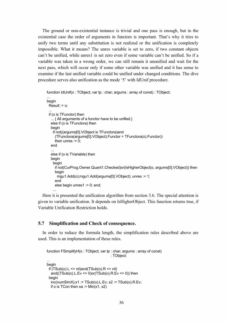
function FSimplifyH(o : TObject; var tp : char; argums : array of const) : TObject;...begin if (TSub(o).L <> nil)and(TSub(o).R <> nil) and((TSub(o).L.Ev <> 0)or(TSub(o).R.Ev <> 0)) then begin inc(numSimX);x1 := TSub(o).L.Ev; x2 := TSub(o).R.Ev; if o is TCon then xa := Min(x1, x2)

37

else if o is TDis then xa := Max(x1, x2) else if o is TImp then xa := Max(-x1, x2) else if o is TEqv then xa := Min(Max(-x1, x2), Max(x1, -x2)); if (xa <> 0) then begin TSub(o).L.RFree; TSub(o).L := nil; TSub(o).R.RFree; TSub(o).R := nil;TSub(o).Ev := xa; { The case, that leads to complete evaluation of a node e.g. (x and true) leads to x .} end else if (xa = 0) then begin negf := 0; if ((o is TImp)and(x2 = -1)) then negf := 1 else if ((o is TEqv)and((x1 = -1)or(x2 = -1))) then negf := 2; if x1 = 0 then o := TSub(o).L.SubstTo else o := TSub(o).R.SubstTo; if negf <> 0 then TSub(o).negate; { The case, that leads to a partial evaluation of a node. e.g. (x and false) leads to false .} end; if TSub(o).neg then TSub(o).Ev := -TSub(o).Ev; end; Result := o;end;

At first it is evaluated the logical value of the subformula o depending on theconnective based on (only for these purposes) three values- false, unknown, true. Then itis decided, whether the subformula will be completely removed or it will be removedonly its descendant.

The decision about the redundancy implements the InsertToR procedure.At first it stores the result of self-resolving on the examined formula. If a logical value

is obtained, check of consequence has no sense. Otherwise it performs the followingactions for every source formula and resolvent until the redundancy is proved. It createsvirtual formula with negated implication in the root, L reference is set up to sourceformula/resolvent root and R reference is set up to the examined formula. It doesn’tcreate any copy and after usage it is restored. It is performed self-resolution byOptimizeX procedure until it has a logical value and if the value is false then the formulais not added to the set of resolvents.

38

C h a p t e r 6

6 Computer application.

6.1 General information.

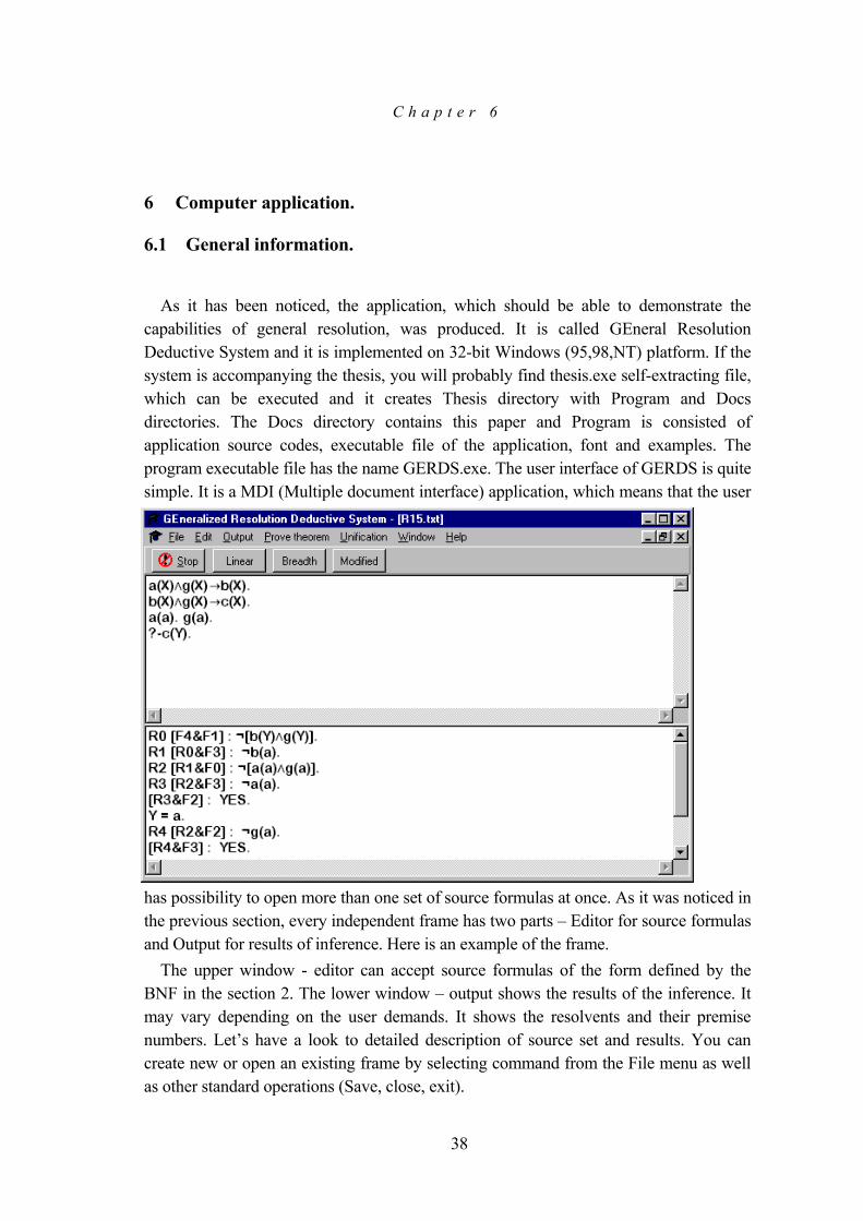
As it has been noticed, the application, which should be able to demonstrate thecapabilities of general resolution, was produced. It is called GEneral ResolutionDeductive System and it is implemented on 32-bit Windows (95,98,NT) platform. If thesystem is accompanying the thesis, you will probably find thesis.exe self-extracting file,which can be executed and it creates Thesis directory with Program and Docsdirectories. The Docs directory contains this paper and Program is consisted ofapplication source codes, executable file of the application, font and examples. Theprogram executable file has the name GERDS.exe. The user interface of GERDS is quitesimple. It is a MDI (Multiple document interface) application, which means that the user

has possibility to open more than one set of source formulas at once. As it was noticed inthe previous section, every independent frame has two parts – Editor for source formulasand Output for results of inference. Here is an example of the frame.

The upper window - editor can accept source formulas of the form defined by theBNF in the section 2. The lower window – output shows the results of the inference. Itmay vary depending on the user demands. It shows the resolvents and their premisenumbers. Let’s have a look to detailed description of source set and results. You cancreate new or open an existing frame by selecting command from the File menu as wellas other standard operations (Save, close, exit).

39

You can use the Window menu to select particular window or reorganize the windoworder. The Help menu gives you essential information about the program and keyboardlayout for special character.

6.2 Input and Output.

The editor (input) window accepts source formulas and goals by syntax of BNF fromthe section 2.1. Source formulas end by dot and one or more blank character ( space,return or other character with ASCII code between 1 and 32). The goal (query) isintroduced by ‘?-‘ string and may occur several times in the editor. Every goal is provedusing all preceding source formulas. Consider next example.

Example 0.1

a(X)ýg(X)ôb(X).b(X)ýg(X)ôc(X).a(a). ?-g(a).g(a).?-c(Y).There are two goals here.

The result (output) window may contain a list of source formulas and goals (alreadynegated), sequence of resolvents, unsimplified forms of resolvents, list of resolvents andsome statistics. The items in the sequence of resolvents are of the form by this example:

Let’s see to an example of the result to the previous source set.

Example 0.2

Source formulas (axioms) :F0 : [a(X)ýg(X)ôb(X)].F1 : [b(X)ýg(X)ôc(X)].F2 : a(a).F3 (¬query) : ¬g(a).______________________________Source formulas (axioms) :F0 : [a(X)ýg(X)ôb(X)].F1 : [b(X)ýg(X)ôc(X)].F2 : a(a).F3 : g(a).F4 (¬query) : ¬c(Y).______________________________R0 [F4&F1] : ¬[b(Y)ýg(Y)].R1 [R0&F3] : ¬b(a).R2 [R1&F0] : ¬[a(a)ýg(a)].R3 [R2&F3] : ¬a(a).[R3&F2] : YES.

40

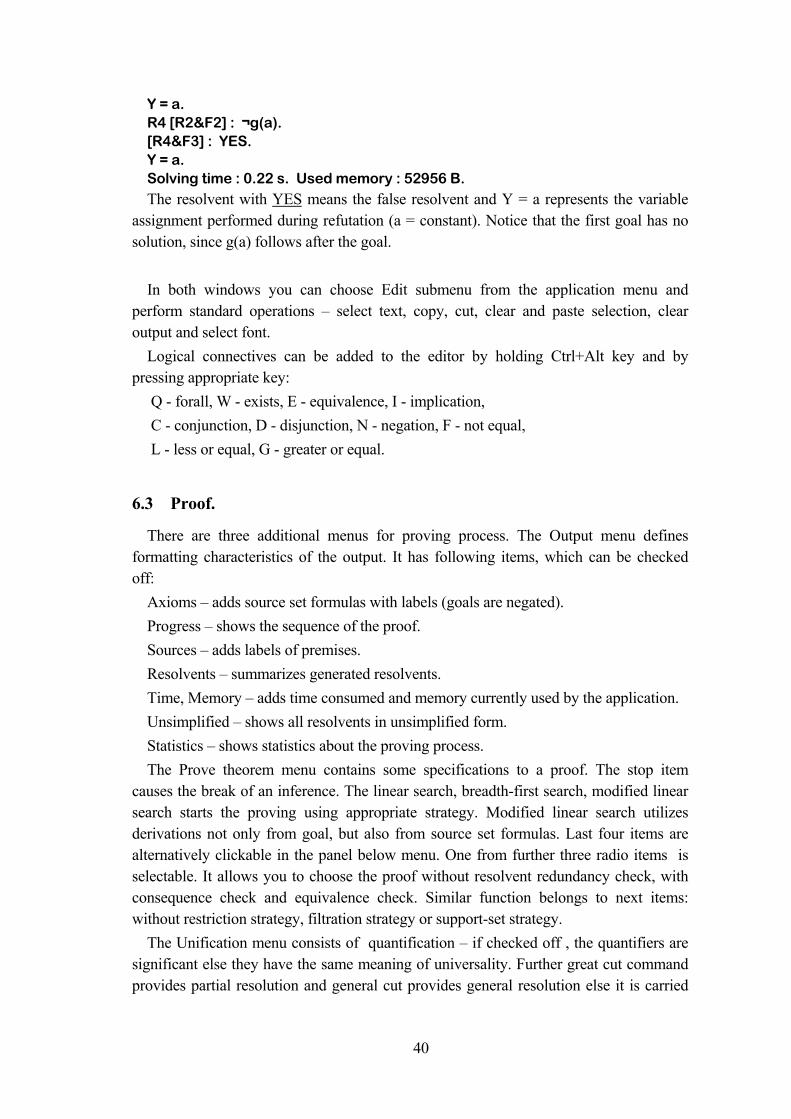
Y = a.R4 [R2&F2] : ¬g(a).[R4&F3] : YES.Y = a.Solving time : 0.22 s. Used memory : 52956 B.The resolvent with YES means the false resolvent and Y = a represents the variable

assignment performed during refutation (a = constant). Notice that the first goal has nosolution, since g(a) follows after the goal.

In both windows you can choose Edit submenu from the application menu andperform standard operations – select text, copy, cut, clear and paste selection, clearoutput and select font.

Logical connectives can be added to the editor by holding Ctrl+Alt key and bypressing appropriate key:

Q - forall, W - exists, E - equivalence, I - implication, C - conjunction, D - disjunction, N - negation, F - not equal, L - less or equal, G - greater or equal.

6.3 Proof.

There are three additional menus for proving process. The Output menu definesformatting characteristics of the output. It has following items, which can be checkedoff:

Axioms – adds source set formulas with labels (goals are negated).Progress – shows the sequence of the proof.Sources – adds labels of premises.Resolvents – summarizes generated resolvents.Time, Memory – adds time consumed and memory currently used by the application.Unsimplified – shows all resolvents in unsimplified form.Statistics – shows statistics about the proving process.The Prove theorem menu contains some specifications to a proof. The stop item

causes the break of an inference. The linear search, breadth-first search, modified linearsearch starts the proving using appropriate strategy. Modified linear search utilizesderivations not only from goal, but also from source set formulas. Last four items arealternatively clickable in the panel below menu. One from further three radio items isselectable. It allows you to choose the proof without resolvent redundancy check, withconsequence check and equivalence check. Similar function belongs to next items:without restriction strategy, filtration strategy or support-set strategy.

The Unification menu consists of quantification – if checked off , the quantifiers aresignificant else they have the same meaning of universality. Further great cut commandprovides partial resolution and general cut provides general resolution else it is carried

41

out the restricted resolution. Next three items determine, how many resolvents have to begenerated from two premises. Exit on first unused creates one resolvents of any type.Exit on first match creates one resolvent, which doesn’t degrade to true or false or whichis not redundant. Exit on last match performs all possible resolution form two premises.Last two items determine if one refutation or all refutations will be done.

42

C h a p t e r 7

7 Examples.

At the end, let’s consider some interesting examples generated by GERDS. We startwith simple propositional examples. All examples were produced using Pentium 100machine.

Example 0.1

Source formulas (axioms) :F0 : a(X). F1 : b(X).F2 (¬query) : ¬[a(X)ýb(X)].______________________________R0 [F2&F1] : ¬a(X).[R0&F0] : YES.R1 [F2&F0] : ¬b(X).[R1&F1] : YES.

Example 0.2

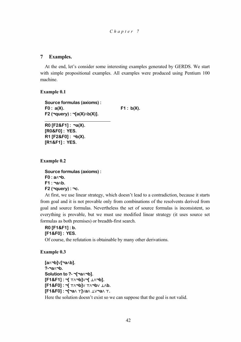
Source formulas (axioms) :F0 : aý¬b.F1 : ¬aýb.F2 (¬query) : ¬c.At first, we use linear strategy, which doesn’t lead to a contradiction, because it starts

from goal and it is not provable only from combinations of the resolvents derived fromgoal and source formulas. Nevertheless the set of source formulas is inconsistent, soeverything is provable, but we must use modified linear strategy (it uses source setformulas as both premises) or breadth-first search.

R0 [F1&F1] : b.[F1&F0] : YES.Of course, the refutation is obtainable by many other derivations.

Example 0.3

[aý¬b]ü[¬aýb].?-¬aý¬b.Solution to ?- ¬[¬aý¬b].[F1&F1] : ¬[ äý¬b]ü¬[ çý¬b].[F1&F0] : ¬[ äý¬b]ü äý¬bü çýb.[F1&F0] : ¬[¬aý ä]üaý çü¬aý ä.Here the solution doesn’t exist so we can suppose that the goal is not valid.

43

Example 0.4

Source formulas (axioms) :F0 : aý¬býcýdü¬aýbý¬cýd.F1 (¬query) : ¬[¬aý¬b].______________________________R0 [F1&F0] : bü¬býcýd.R1 [F1&F0] : aü¬aý¬cýd.R2 [F0&F0] : bý¬cýdü¬býcýd.R3 [F0&F0] : ¬aý¬cýdüaýcýd.R4 [F0&F0] : ¬aýbýdüaý¬býd.R5 [F0&F0] : aý¬býcü¬aýbý¬c.It is the next example of a goal, which is not provable.

Example 0.5

Source formulas (axioms) :F0 : aôbýg. F1 : býgôc. F2 : býgôa. F3 : côbýg.F4 (¬query) : ¬[aóc].______________________________R0 [F4&F3] : aübýg. R1 [R0&F4] : býgü¬c.R2 [R1&F2] : ¬cü[gôa]. R3 [R2&F1] : [gôa]ü¬[býg].R4 [R3&F4] : ¬gü¬[býg]ü¬c. R5 [R4&F3] : ¬bü¬c.R6 [R5&F4] : ¬büa. R7 [R6&F3] : aü¬c.R8 [R7&F4] : ¬c. R9 [R8&F4] : a.R10 [R9&F0] : býg. R11 [R10&F1] : gôc.R12 [R11&F4] : ¬gü¬a. R13 [R12&F0] : ¬a.R14 [R13&F4] : c. [R14&R8] : YES.Solving time : 0.48 s.

Source formulas (axioms) :F0 : aóbýg. F1 : býgóc. F2 (¬query) : ¬[aóc].______________________________R0 [F2&F1] : [¬aü¬[býg]]ý[aübýg]. R1 [R0&F2] : ¬[býg]üc.R2 [R1&F0] : ¬gücü¬a. R3 [R2&F2] : ¬gü¬a.R4 [R3&F2] : ¬güc. R5 [R4&F0] : cü¬a.R6 [R5&F2] : ¬a. R7 [R6&F2] : c.R8 [R7&F1] : býg. R9 [R8&F1] : góc.R10 [R9&F2] : [güa]ý[¬gü¬a]. R11 [R10&F1] : aü[bóc].R12 [R11&F1] : aü¬cü¬g. R13 [R12&F2] : ¬cü¬g.R14 [R13&F2] : ¬güa. R15 [R14&F1] : aü¬c.R16 [R15&F2] : ¬c. R17 [R16&F2] : a.[R17&R6] : YES.Solving time : 0.54 s.

Last two inferences were an example of strongly non-clausal resolution. As stated, theproof of aóc can be done both from implicative and equivalence based axioms.

44

Example 0.6

F0 : [a(X)ýg(X)ôb(X)].F1 : a(a).F2 : g(c).F3 (¬query) : ¬b(a).______________________________R0 [F3&F0] : ¬[a(a)ýg(a)].R1 [R0&F1] : ¬g(a).Solving time : 0.06 s.b(a) is not provable, because g(a) doesn’t hold. When we add it, the proof exists.

Source formulas (axioms) :F0 : [a(X)ýg(X)ôb(X)]. F1 : a(a).F2 : g(c). F3 : g(a).F4 (¬query) : ¬b(a).______________________________R0 [F4&F0] : ¬[a(a)ýg(a)]. R1 [F3&F0] : [a(a)ôb(a)].R2 [F2&F0] : [a(c)ôb(c)]. R3 [F1&F0] : [g(a)ôb(a)].R4 [R3&F4] : ¬g(a). R5 [R3&F3] : b(a).R6 [R1&F4] : ¬a(a). [R6&F1] : YES.Solving time : 0.27 s.There are interesting resolvents with implication, which show the lucidity of the proof

(in contrast with clausal resolution), in this breadth-first search proof above.

Example 0.7

Source formulas (axioms) :F0 : [a(X)ýg(X)ôb(X)]. F1 : [b(X)ýg(X)ôc(X)].F2 : a(a). F3 : g(a).F4 (¬query) : ¬c(Y).______________________________R0 [F4&F1] : ¬[b(Y)ýg(Y)]. R1 [F3&F1] : [b(a)ôc(a)].R2 [F3&F0] : [a(a)ôb(a)]. R3 [F2&F0] : [g(a)ôb(a)].R4 [F1&F0] : [[g(X)ôc(X)]ü¬[a(X)ýg(X)]].R5 [R4&F4] : [¬g(X)ü¬[a(X)ýg(X)]]. R6 [R4&F3] : [c(a)ü¬a(a)].R7 [R3&F3] : b(a). R8 [R3&F1] : [¬g(a)üc(a)].R9 [R3&R0] : ¬g(a). R10 [R1&F4] : ¬b(a).R11 [R1&R7] : c(a). [R11&F4] : YES. Y = a.[R10&R7] : YES. Y = a.R12 [R10&R2] : ¬a(a).[R9&F3] : YES. Y = a.[R7&R10] : YES. Y = a.[R12&F2] : YES. Y = a.Solving time : 1.72 s.

45

This example is the first one with a goal requiring variables. There were fivepossibilities to refute the source set.

Example 0.8

Source formulas (axioms) :F0 : [a(X)ôa(X+1)]. F1 : a(0).F2 (¬query) : ¬a(5).______________________________R0 [F1&F0] : a(1). R1 [R0&F0] : a(2).R2 [R1&F0] : a(3). R3 [R2&F0] : a(4).R4 [R3&F0] : a(5). [R4&F2] : YES.Solving time : 0.05 s.This is a sample of the usage of infix operators.

Example 0.9

Source formulas (axioms) :F0 : 1<2. F1 : 2<3.F2 : 3<4. F3 : 4<5.F4 : 5<6. F5 : [X<YýY<ZôX<Z].F6 (¬query) : ¬1<5.______________________________R0 [F6&F5] : ¬[1<YýY<5]. R1 [R0&F3] : ¬1<4.R2 [R1&F5] : ¬[1<YýY<4]. R3 [R2&F2] : ¬1<3.R4 [R3&F5] : ¬[1<YýY<3]. R5 [R4&F1] : ¬1<2.[R5&F0] : YES.Solving time : 0.22 s.This proof illustrates transitivity, which is well solved by the application.

Example 0.10

Source formulas (axioms) :F0 : [a(X)ýg(Z)ôb(X)]. F1 : [b(X)ýg(Z)ôc(X)].F2 : a(a). F3 : g(30).F4 (¬query) : ¬[c(Y)üg(Y)üb(Y)].______________________________R0 [F4&F4] : ¬[g(Y)üb(Y)]. R1 [F4&F4] : ¬[c(Y)üb(Y)].R2 [F4&F4] : ¬[c(Y)üg(Y)].[F4&F3] : YES. Y = 30.[F3&F4] : YES. Y = 30.R3 [F3&F0] : [a(X)ôb(X)]. R4 [R3&F4] : ¬a(X).R5 [R3&F2] : b(a).[R2&F3] : YES. Y = 30.[R1&R5] : YES. Y = a.[R0&F3] : YES. Y = 30.[R0&R5] : YES. Y = a.[R5&F4] : YES. Y = a.

46

[R5&R1] : YES. Y = a.[R5&R0] : YES. Y = a.[R4&F2] : YES. Y = a.Solving time : 0.54 s.

Next example produces the Fibonacci sequence.

Example 0.11

Source formulas (axioms) :F0 : [f(I, A) ý f(I+1, B) ô f(I+2, A+B)].F1 : f(0, 1). F2 : f(1, 1).F3 (¬query) : ¬f(15, X).______________________________R0 [F2&F0] : [f(2, B)ôf(3, 1+B)]. R1 [F1&F0] : [f(1, B)ôf(2, 1+B)].R2 [R1&F2] : f(2, 2). R3 [R0&R2] : f(3, 3).R4 [R3&F0] : [f(4, B)ôf(5, 3+B)]. R5 [R2&F0] : [f(3, B)ôf(4, 2+B)].R6 [R5&R3] : f(4, 5). R7 [R4&R6] : f(5, 8).R8 [R7&F0] : [f(6, B)ôf(7, 8+B)]. R9 [R6&F0] : [f(5, B)ôf(6, 5+B)].R10 [R9&R7] : f(6, 13). R11 [R8&R10] : f(7, 21).R12 [R11&F0] : [f(8, B)ôf(9, 21+B)]. R13 [R10&F0] : [f(7, B)ôf(8, 13+B)].R14 [R13&R11] : f(8, 34). R15 [R12&R14] : f(9, 55).R16 [R15&F0] : [f(10, B)ôf(11, 55+B)].R17 [R14&F0] : [f(9, B)ôf(10, 34+B)].R18 [R17&R15] : f(10, 89). R19 [R16&R18] : f(11, 144).R20 [R19&F0] : [f(12, B)ôf(13, 144+B)].R21 [R18&F0] : [f(11, B)ôf(12, 89+B)].R22 [R21&R19] : f(12, 233). R23 [R20&R22] : f(13, 377).R24 [R23&F0] : [f(14, B)ôf(15, 377+B)].R25 [R22&F0] : [f(13, B)ôf(14, 233+B)].R26 [R25&R23] : f(14, 610). R27 [R24&R26] : f(15, 987).[R27&F3] : YES. X = 987.Solving time : 1.29 s.We found the fifteenth Fibonacci number, which is 987 (if zero number is 1).

Another known sequence may be produced using factorial function.Source formulas (axioms) :F0 : [f(X, Y)ôf(X+1, Y*(X+1))]. F1 : f(1, 1).F2 (¬query) : ¬f(10, Y).______________________________R0 [F1&F0] : f(2, 2). R1 [R0&F0] : f(3, 6).R2 [R1&F0] : f(4, 24). R3 [R2&F0] : f(5, 120).R4 [R3&F0] : f(6, 720). R5 [R4&F0] : f(7, 5040).R6 [R5&F0] : f(8, 40320). R7 [R6&F0] : f(9, 362880).R8 [R7&F0] : f(10, 3628800).[R8&F2] : YES. Y = 3628800.

47

Now let’s have a look into simple quantified examples. As it was noticed, these simpleexamples are workable by the application.

At first, consider several combinations of the base case, which illustrate the behaviourof existential variables.

Example 0.12

F0: ÷XöY p(X,Y).?-öY÷X p(X,Y). ?-öYöX p(X,Y). ?-÷XöY p(X,Y). ?-÷Y÷X p(X,Y).Solution to #1.Solution to #2.[F1&F0] : YES.Solution to #3.[F1&F0] : YES.Solution to #4.

Case 1 and 4 have no solution, since they do not imply from F0. The opposite casefollows.

öY÷X p(X,Y).?-÷XöY p(X,Y). ?-öXöY p(X,Y). ?-÷X÷Y p(X,Y).Solution to #1.[F1&F0] : YES.Solution to #2.[F1&F0] : YES.Solution to #3.

Here case 1 and 2 lead to refutation. If we change the axiom, this result is obvious.

öYöX p(X,Y).?-÷XöY p(X,Y). ?-öXöY p(X,Y). ?-÷X÷Y p(X,Y).Solution to #1.Solution to #2.[F1&F0] : YES.Solution to #3.

These examples show the simplest cases, but now let’s have a look into morecomplicated instance, where it is needed to perform more than one pass to unify twoatoms.

Example 0.13

÷ZöY p(X,Y,Z). ?- ÷ZöY p(X,Y,Z).[F1&F0] : YES.The unifying algorithm strikes on a problem, when it unifies these two atoms. It takes

X without problems, but when it tries to substitute universal Y (with respect to polarity!)

48

from F1, the existential Y from F0 has one superior variable Z. Z is not substituted yet,so we temporarily continue with next argument - Z variable. It can be substituted withexistential Z (which has no superior variable) and then the next pass follows. In thispass, we are able to substitute Y, since Z is already substituted.

Next samples show instances similar to example 7.12.÷ZöY p(X,Y,Z). ?- öY÷Z p(X,Y,Z).Solution to #1.andöY÷Z p(X,Y,Z). ?- ÷ZöY p(X,Y,Z).Solution to #1.[F1&F0] : YES.

Example 0.14

This example is an illustration of more complicated formulas with existentialvariables.

÷X a(X) ô öX b(X). ÷X a(X).?- b(a).Solution to ¬b(a).

öX a(X)ô÷X b(X). a(a).?- b(c).Solution to ¬b(c).R0 [F2&F0] : ÷X ¬a(X).[R0&F1] : YES.

49

C h a p t e r 8

8 Conclusions.

The last chapter analyzed some examples, which were the best approach for reader tounderstand the theoretical power of general resolution. Although the general resolutionis not efficient in comparison with clausal and Horn logic, it preserves the sequence ofthe proof. Achieved solving times are controversial. It is obvious, that these times growquicker than for clauses. Even if we use some techniques of avoiding redundancy, theefficiency is still low for the serious usage in knowledge representation. Nevertheless,the proposed theoretical system may be a good source of training for persons interestedin deductive systems as well as in logic generally.

The existence handling methods are partially satisfied in the application, which is oneof the results of the thesis, and they were shown in examples as functional extensions ofground general resolution. Also the check of consequence by self-resolution, which wasproposed by the thesis, is strong result making the proving by general resolutionapplicable to machine-performed deduction and not only applicable for intuitive human-performed proofs.

There are many further problems in theorem-proving and resolution techniques as itsmain branch. That’s why the thesis may lead to continual research in theory of resolutionas well as in progressive sectors of logic (Fuzzy logic, Objective-oriented logics).Though it will not continue directly, it is an excellent starting point for designing anotherknowledge-based systems, which, I believe, will be the objective of my future work. Itlies mainly in programming the application. It wasn’t an easy job to design and realizethe GERDS and unfortunately, it is not so visible result as I imagined. The importantcontribution of the thesis is to remind, that there are essential items in logic, that are notemphasized in conventional studies, and it is interesting to deal with them.

50

REFERENCES

9 References.

[Ba97] Bachmair L., Ganzinger H.: A theory of resolution. Technical report of the

Max-Planck-Institut für Informatik, 1997.

[Be71] Berztiss A.T.: Data structures. Academic press, 1971.

[Ce81] Čechák V.: Co víte o moderní logice. Horizont, 1981.

[Dv92] Dvořák S.: Dekompozice a rekurzivní algoritmy. Grada, 1992.

[Ji88] Jinoch J., a kol.: Programování v jazyku Pascal. SNTL, 1988.

[Kl67] Kleene S.C. Mathematical logic. John Willey & Sons, 1967.

[Lu95] Lukasová A.: Logické základy umělé inteligence. Učební texty Ostravské

Univerzity, 1995,1997.

[Ma93] Mařík V., Štěpánková O., Lažanský J.: Umělá Inteligence (1), (2).

Academia 1993,1997

[No90] Novák, V.: Fuzzy množiny a jejich aplikace. SNTL, 1990.

[Ri89] Richards T.: Clausal Form Logic. Addison-Wesley,1989.