Dana JoaquinECE 3522: StochasticsDepartment of Electrical and Computer Engineering, Temple University, Philadelphia, PA 19121

I. PROBLEM STATEMENT

The purpose of this assignment is to explore the concept of signal-to-noise ratio (SNR) and analyzing its autocorrelation function and its power spectral density. This will be done by analyzing a signal that is a sum of a sinusoid and noise by varying its SNR value. The given parameters to do this assignment are:

Amplitude of sinewave is +/- 1 SNR range of -30 to 30 dB in steps of 10 dB τ = 16 lags sinewave is 500 Hz signal is sampled at 8000 Hz

II. APPROACH AND RESULTS

The functions that were used extensively in this assignment were MATLAB’s autocorr and fft functions. The autocorr function computes the autocorrelation function of a signal given the number of lags and the fft function computes the fast Fourier transform of a signal. One of the requirements of the assignment was to create a custom function that generate the sinewave with the noise called “generate_sine” that took in four arguments: frequency of the sinewave, duration of sinewave in seconds, sampling frequency and the SNR ratio in dB. The algorithm of the function was taken from the SNR page on the MathWorks website. How the generate_sine function worked is that it computed the power of the sinewave and then the power of the noise based on the inputted SNR value. Since the amplitude of the sinusoid is assumed to be +/- 1 and that it is a periodic sinusoid, the equation to calculate its power is:

Ps=A2

2=1

2,=amplitudeof sinusoid

Equation 1. Average Power of Periodic Sinusoid

Once Ps was calculated and given the SNR dB value, the noise power, Pn, can be calculated by deriving its equation from the SNR equation.

SNRdB=20 log10

PsPN

Equation 2. SNR equation in dB

PN=P s

10SNR dB

20

Equation 3. Derived Noise Power Equation from Equation 2

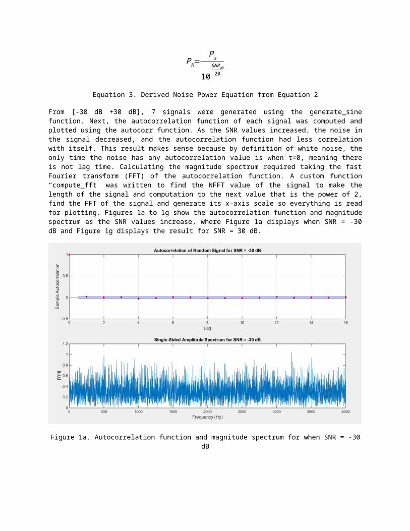
From [-30 dB +30 dB], 7 signals were generated using the generate_sine function. Next, the autocorrelation function of each signal was computed and plotted using the autocorr function. As the SNR values increased, the noise in the signal decreased, and the autocorrelation function had less correlation with itself. This result makes sense because by definition of white noise, the only time the noise has any autocorrelation value is when τ=0, meaning there is not lag time. Calculating the magnitude spectrum required taking the fast Fourier transform (FFT) of the autocorrelation function. A custom function “compute_fft” was written to find the NFFT value of the signal to make the length of the signal and computation to the next value that is the power of 2, find the FFT of the signal and generate its x-axis

scale so everything is read for plotting. Figures 1a to 1g show the autocorrelation function and magnitude spectrum as the SNR values increase, where Figure 1a displays when SNR = -30 dB and Figure 1g displays the result for SNR = 30 dB.

Figure 1a. Autocorrelation function and magnitude spectrum for when SNR = -30 dB

Figure 1b. Autocorrelation function and magnitude spectrum for when SNR = -20 dB

Figure 1c. Autocorrelation function and magnitude spectrum for when SNR = -10 dB

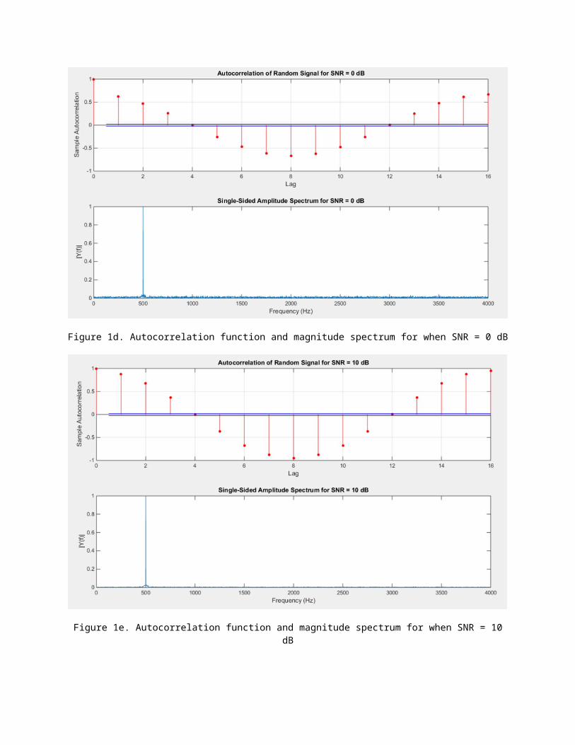
Figure 1d. Autocorrelation function and magnitude spectrum for when SNR = 0 dB

Figure 1e. Autocorrelation function and magnitude spectrum for when SNR = 10 dB

Figure 1f. Autocorrelation function and magnitude spectrum for when SNR = 20 dB

Figure 1g. Autocorrelation function and magnitude spectrum for when SNR = 30 dB

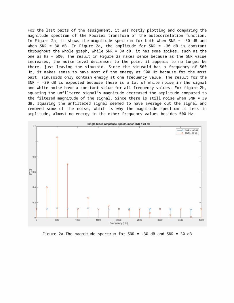
For the last parts of the assignment, it was mostly plotting and comparing the magnitude spectrum of the Fourier transform of the autocorrelation function. In Figure 2a, it shows the magnitude spectrum for both when SNR = -30 dB and when SNR = 30 dB. In Figure 2a, the amplitude for SNR = -30 dB is constant throughout the whole graph, while SNR = 30 dB, it has some spikes, such as the one as Hz = 500. The result in Figure 2a makes sense because as the SNR value increases, the noise level decreases to the point it appears to no longer be there, just leaving the sinusoid. Since the sinusoid has a frequency of 500 Hz, it makes sense to have most of the energy at 500 Hz because for the most part, sinusoids only contain energy at one frequency value. The result for the SNR = -30 dB is expected because there is a lot of white noise in the signal and white noise have a constant value for all frequency values. For figure 2b, squaring the unfiltered signal’s magnitude decreased the amplitude compared to the filtered magnitude of the signal. Since there is still noise when SNR = 30 dB, squaring the unfiltered signal seemed to have average out the signal and removed some of the noise, which is why the magnitude spectrum is less in amplitude, almost no energy in the other frequency values besides 500 Hz.

Figure 2a.The magnitude spectrum for SNR = -30 dB and SNR = 30 dB

Figure 2b. The magnitude spectrum for the original SNR = 3 dB and its filtered version.

III. MATLAB CODE

% computer assignment 9

% Dana Joaquin function ca09_v00 clear; clcclose all % parametersFs = 8e3; % sampling frequencyt = 1; % length of signal in time (seconds)snrdb = -30:10:30; % SNRfq = 500; % signal frequencylagt = 16; % # of lags for autocorrelation calculation for i=1:length(snrdb) % generating random signal [nsig, tym] = gen_sine(fq, t, Fs, snrdb(i)); % computing autocorrelation figure(i) subplot(2, 1, 1) autocorr(nsig, lagt); titlestring = sprintf('Autocorrelation of Random Signal for SNR = %d dB', snrdb(i)); title(titlestring) % FFT of signal subplot(2, 1, 2) [Y1, f1, NFFT1] = compute_fft(length(tym), nsig, Fs); plot(f1, 2*abs(Y1(1:NFFT1/2+1))) titlestring = sprintf('Single-Sided Amplitude Spectrum for SNR = %d dB', snrdb(i)); title(titlestring) xlabel('Frequency (Hz)') ylabel('|Y(f)|') if i == 1 % save nsig at -30 dB for other part of assignment nsigneg30 = nsig; end if i == length(snrdb) % save nsig at 30 dB for last part of assignment nsig30 = nsig; endend % autocorr of filtered signalac = autocorr(nsigneg30, lagt); % computing FT of autocorr data & plotting magnitude[Y, f, NFFT] = compute_fft(length(ac), ac, Fs);figure(1+length(snrdb))stem(f, 2*abs(Y(1:NFFT/2+1)))title('Single-Sided Amplitude Spectrum for SNR = 30 dB')xlabel('Frequency (Hz)')ylabel('|Y(f)|')hold onac = autocorr(nsig30, lagt); % computing FT of autocorr data & plotting magnitude[Y, f, NFFT] = compute_fft(length(ac), ac, Fs);stem(f, 2*abs(Y(1:NFFT/2+1))) % parametersA = 0.5; % feedback coefficientsB = 1; % feedforward coefficientsy = filter(B, A, nsig30); % filtering signal % autocorr of filtered signalac = autocorr(y, lagt); % computing FT of autocorr data & plotting magnitude

[Y2, f2, NFFT2] = compute_fft(length(ac), ac, Fs);figure(2+length(snrdb))stem(f2, 2*abs(Y2(1:NFFT2/2+1)))title('Single-Sided Amplitude Spectrum for SNR = 30 dB')xlabel('Frequency (Hz)')ylabel('|Y(f)|') hold on% computing autocorr of original signal, nsig30ac = autocorr(nsig30, lagt);% computing FT of autocorr data of nsig30 & plotting magnitude^2[Y3, f3, NFFT3] = compute_fft(length(ac), ac, Fs);stem(f3, (2*abs(Y3(1:NFFT3/2+1)).^2))legend('filtered', 'unfiltered') end % function name: compute_fft% coded by Dana Joaquin% input argument(s):% (1) siglength: length of signal (scalar)% (2) sigg: signal data (vector)% (3) samplf: sampling frequency of signal (scalar)% output argument(s):% (1) fftresult: data of FT signal (vector)% (2) fftscale: length of FT signal (vector)% (3) nfft: length of FT signal to nearest power of 2 (scalar)% objective:% This function computes the fast Fourier transform of a signal% by first calculating the NFFT of the signal to get the scale% of the FT result to closest power of 2 value to scale the% result for plotting.% function [fftresult, fftscale, nfft] = compute_fft(siglength, sigg, sampf) nfft = 2^nextpow2(siglength); % NFFT value to scale signalfftresult = fft(sigg, nfft)/siglength; % FT result of signalfftscale = sampf/2*linspace(0,1,nfft/2+1); % x-scale vector of FT signal end % function name: gen_sine% coded by Dana Joaquin% input argument(s):% (1) vect: signal data (array)% (2) nmatrix: size of the desired square matrix% output argument(s):% (1) sig: resulting sinusoid signal with noise% (2) time: time scale vector of signal% objective:% This function generates a sinewave with noise, assuming an% amplitude of +/- 1 for the sinewave portion. The general algorithm% for this function was taken off of the SNR page of the% MathWorks website:% http://www.mathworks.com/help/signal/ref/snr.html%function [sig, time] = gen_sine(freq, T, fs, snr_db) rng defaultA = 1.0; % amplitude of sinewaveps = A^2/2; % power of signalden = 10^(snr_db/20);pn = ps/den; % calculating power of noise % generating time vector of signaltime = 0:1/fs:T-1/fs;

% checks calculated pn if give back snr_db value% c = 20*log10(ps/pn); % generate sinusoidsig = A*cos(2*pi*freq*time) + pn*randn(size(time)); end

IV. CONCLUSIONS

Based on the results of the assignment, the more negative the SNR value is in dB, the more noise is added to the signal. This makes sense because when computing the log of the dB value of SNR, when taking the log of a negative value, it ends up being a decimal value that is less than 1 but greater than 0. From the results of the math, the more the ratio between the noise and signal is closer to 0, the more noise is in the signal. Again, this makes sense because the smaller the ratio, the more they have no relation to each other to the point that there appears to be no ratio at all between the actual signal and noise. However, as the SNR value increases, having a larger ratio shows that the sinusoid and the noise have more of mathematical relation, therefore they correlate more, which is evident as the SNR value increases. Therefore, when the SNR value is 0 dB, it is saying the signal and the noise are essentially 1:1 since the log of 1 is 0.

The Fourier transform of white noise’s autocorrelation function results in constant amplitude throughout all frequencies. This is expected since its autocorrelation function only had a nonzero value at τ=0 and everywhere else it was zero, meaning it was an impulse function and impulse functions result with a constant value for all frequencies in the frequency domain. The Fourier transform of the autocorrelation function is the power spectral density of the signal and for white noise, it has energy in all frequencies, which matches the result that was computed.

For the last part of the assignment and the last plot, when the signal is filtered through the digital filter, when compared to the result in figure 2a, it appears that nothing changed for the signal. However, when the unfiltered signal’s magnitude was squared, its amplitude decreases compared to the filtered one. They have impulses at the same frequency values, but they differ in amplitude. For the unfiltered result, squaring the magnitude appeared to filter the signal, decreases its amplitude and removing the other amplitude values from the larger frequencies, as though squaring the signal averaged it or squaring the signal seemed like low-pass filtering it. Squaring it seemed to have remove the white noise components of the signal, leaving only the sinusoid part since at 500 Hz, it has the most amount of energy.