Original Article Air recovery assessment on high-pressure pneumatic systems Jose ´ A Trujillo, Pedro J Gamez-Montero and Esteban Codina Macia `v Abstract A computational simulation and experimental work of the fluid flow through the pneumatic circuit used in a stretch blow moulding machine is presented in this paper. The computer code is built around a zero-dimensional thermodynamic model for the air blowing and recycling containers together with a non-linear time-variant deterministic model for the pneumatic three stations single acting valve manifold, which, in turn, is linked to a quasi-one-dimensional unsteady flow model for the interconnecting pipes. The flow through the pipes accounts for viscous friction, heat transfer, cross-sectional area variation, and entropy variation. Two different solving methods are applied: the method of charac- teristics and the HLL Riemann first-order scheme. The numerical model allows prediction of the air blowing process and, more significantly, permits determination of the recycling rate at each operating cycle. A simplified experimental set-up of the industrial process was designed, and the pressure and temperature were adequately monitored. Predictions of the blowing process for various configurations proved to be in good agreement with the measured results. In addition, a novel design of a valve manifold intended for the polyethylene terephthalate (PET) plastic bottle manufacturing industry is also presented. [AQ1] Keywords Air recycling system, energy assessment, air blow moulding manufacturing process, pneumatic valve manifold Date received: 6 November 2015; accepted: 10 March 2016 Introduction Despite the many contributions linked to energy con- servation in pneumatic systems, no publications report the efficiency on high-pressure pneumatic applications. [AQ2]In order to bring some light to this issue, it is crucial to get into the patents published during the last 20 years. Amongst various industrial applications that require high-pressure air, polyethylene terephthalate (PET) stretch blow moulding machine manufacturers have contributed significantly to enhancing energy effi- ciency in that specific field of pneumatic systems. In 1981 Air Products and Chemicals Inc. 1 pub- lished a patent related to a process for the production of blow moulded articles in which the blowing gas was recovered and treated to be used in subsequent moulding operations. A year later Robert Bosch GmbH suggested recovering the compressed air used in the moulding operation to feed other pneumatic applications. A similar proposal was provided by The Continental Group Inc. 2 in 1984, which was sub- sequently taken as a reference by other blow moulding bottle manufacturers. In 1995 Krupp Corpoplast Maschinenbau GmbH 3,4 presented an invention that recovered part of the air used for moulding a container made of thermoplastic material. The high- pressure blowing air was supplied to the low-pressure air supply during a transitional phase by employing a reversing mechanism. An invention that has been cited by several blowing machine manufacturers is the patent of Procontrol AG (1996), 5 which proposed to produce the high-pressure air adiabatically while the low-pressure air was generated isothermically, thus enabling the entire blowing process to be carried out with the smallest possible amount of energy. Over the same period and based on the same principle, A.K. Tech Lab Inc. (1997) 6 proposed recovering the exhaust air into a tank that later supplied air to oper- ate secondary pneumatic circuits. In order to compen- sate for the difference between the recovered air and that consumed by the installation, a compressor LABSON, Campus Terrassa, UPC, Terrassa, Barcelona, Spain Corresponding author: Jose ´ A Trujillo, Escuela Tcnica Superior de Ingenieras Industrial y Aeronutica de Terrassa, Campus de Terrassa, Edificio TR5, C/ Colom, 11 Terrassa, 08222 Spain. Email: [email protected]Proc IMechE Part C: J Mechanical Engineering Science 0(0) 1–12 ! IMechE 2016 Reprints and permissions: sagepub.co.uk/journalsPermissions.nav DOI: 10.1177/0954406216645823 pic.sagepub.com
Transcript
Original Article
Air recovery assessment onhigh-pressure pneumatic systems
Jose A Trujillo, Pedro J Gamez-Monteroand Esteban Codina Maciav
Abstract
A computational simulation and experimental work of the fluid flow through the pneumatic circuit used in a stretch blow
moulding machine is presented in this paper. The computer code is built around a zero-dimensional thermodynamic
model for the air blowing and recycling containers together with a non-linear time-variant deterministic model for
the pneumatic three stations single acting valve manifold, which, in turn, is linked to a quasi-one-dimensional unsteady
flow model for the interconnecting pipes. The flow through the pipes accounts for viscous friction, heat transfer,
cross-sectional area variation, and entropy variation. Two different solving methods are applied: the method of charac-
teristics and the HLL Riemann first-order scheme. The numerical model allows prediction of the air blowing process and,
more significantly, permits determination of the recycling rate at each operating cycle. A simplified experimental set-up of
the industrial process was designed, and the pressure and temperature were adequately monitored. Predictions of the
blowing process for various configurations proved to be in good agreement with the measured results. In addition, a
novel design of a valve manifold intended for the polyethylene terephthalate (PET) plastic bottle manufacturing industry is
also presented. [AQ1]
Keywords
Air recycling system, energy assessment, air blow moulding manufacturing process, pneumatic valve manifold
Date received: 6 November 2015; accepted: 10 March 2016
Introduction
Despite the many contributions linked to energy con-servation in pneumatic systems, no publications reportthe efficiency on high-pressure pneumatic applications.[AQ2]In order to bring some light to this issue, it iscrucial to get into the patents published during the last20 years. Amongst various industrial applications thatrequire high-pressure air, polyethylene terephthalate(PET) stretch blow moulding machine manufacturershave contributed significantly to enhancing energy effi-ciency in that specific field of pneumatic systems.
In 1981 Air Products and Chemicals Inc.1 pub-lished a patent related to a process for the productionof blow moulded articles in which the blowing gas wasrecovered and treated to be used in subsequentmoulding operations. A year later Robert BoschGmbH suggested recovering the compressed air usedin the moulding operation to feed other pneumaticapplications. A similar proposal was provided byThe Continental Group Inc.2 in 1984, which was sub-sequently taken as a reference by other blow mouldingbottle manufacturers. In 1995 Krupp CorpoplastMaschinenbau GmbH3,4 presented an invention thatrecovered part of the air used for moulding a
container made of thermoplastic material. The high-pressure blowing air was supplied to the low-pressureair supply during a transitional phase by employing areversing mechanism. An invention that has beencited by several blowing machine manufacturers isthe patent of Procontrol AG (1996),5 which proposedto produce the high-pressure air adiabatically whilethe low-pressure air was generated isothermically,thus enabling the entire blowing process to be carriedout with the smallest possible amount of energy. Overthe same period and based on the same principle,A.K. Tech Lab Inc. (1997)6 proposed recovering theexhaust air into a tank that later supplied air to oper-ate secondary pneumatic circuits. In order to compen-sate for the difference between the recovered air andthat consumed by the installation, a compressor
provided sufficient air to balance the pressure in thetank. Also, the proposal of Asahi Kasei KogoyoKabushiki Kaisha (1993)7 must be taken into account,which added a recovery container from which the com-pressed gas could be aspirated by a multistage com-pressor. In 2003 Technoplan8 published an inventionwhich targeted the optimization of the above-men-tioned methods. A relevant improvement was the factthat the recovered gas (17 bar) was expanded beforebeing used in the low-pressure air phase, which meantthat it did not have influence on the low-pressure air atthe time of its use. On the other hand, several proposalswere given to re-use the recovered air, such as actuatingthe preform-stretching rams, actuating consumablesof the packaging-production machine, or even return-ing the recycled gas to the compressed air network. Themethod allowed around 20% to 45% of air recoveryand a reduction of electrical power consumption of15% to 45%.
[AQ3]Based on the existing state of the art it maybe concluded that even though numerous attempts
have been made to improve the efficiency of air blow-ing pneumatic systems, there are no previous publica-tions which focused specifically on analysing thecomplexity of this particular industrial field.Therefore, this investigation aims to determine themain constraints that limit the efficiency of a blowmoulding plastic PET bottle pneumatic circuit withthe help of a computational model which is able topredict the maximum amount of recycled air that maybe ensured at each operating cycle. Moreover, thistool will not only contribute to assessing the efficiencyof the air blowing machine but will also allow re-designing of the regpneumatic lay-out to minimizethe energy losses.9
Mathematical model of the air blowmoulding pneumatic system [AQ4]
Due to the complexity of the air blow mouldingmachine, the pneumatic circuit has been reduced tothe pneumatic scheme depicted in Figure 1, resulting
Figure 1. [AQ30]Single station PET bottle production pneumatic scheme with air recovery system. [AQ5]
2 Proc IMechE Part C: J Mechanical Engineering Science 0(0)
in three individual submodels, which are representedby the fluid flow through the pipes, the charging anddischarging process from/to the vessels and the fluiddynamics inside the valve manifold. The valve mani-fold is supplied with two different pressures, and aspecial cylinder is responsible for providing com-pressed air to the plastic preform through a hollowedstretching rod. From the patents mentioned in theprevious section we learned that once the plasticbottle is produced, the air inside the container is par-tially recycled while the remaining fluid is exhaustedto the atmosphere once the air level inside the recy-cling chamber reaches a certain pressure. It must bepointed out that the main scope of this study does nottake into account the deformation of the preformduring the blowing process, but the amount of airthat is needed to produce the bottle. As a matter offact the pressure characteristics inside the mould willbehave slightly differently in a real blow mouldingmachine. On the other hand, for the sake of simplicitythe simulation will omit the components locatedbefore the valve manifold, such as the filter and pres-sure regulator.
The recycling stage always takes place after closingV1 (refer to Figure 1). At this point the air flowsthrough the pipe connecting the cavity chamber andthe manifold, and circulates through the valve mani-fold until it reaches the recycling chamber. At a cer-tain stage, the air in the recycling chamber equalizesthe pressure in the cavity chamber, being the pointwhen the recycling process ends, and the remainingair in the cavity chamber is released to the atmos-phere. As a matter of fact, the use of an additionalrecycling process may be also considered at this point,however, a different concept design of the valve mani-fold should be used. It must be noted that the amountof energy available in the cavity chamber drops as thepressure decreases so an additional recycling stageshould be considered.
Mathematical model at the pipes
The flow through the pipes connecting the differentunits has been considered quasi-one-dimensional andthe methods implemented in order to determine thecharacteristics of the fluid flow have been the methodof characteristics (MOC)10,11 and the HLL Riemannsolver12–14 respectively. [AQ6] Both models wereimplemented in Fortran and only differed in the waythat the governing equations were solved. The simu-lations were run on a x86 (32-bit) architecturePentium processor with a dual Intel Core QuadCPU 2.4 GHz processor and 3.0 GB memory.
Zero-dimensional thermodynamic volume
The performance of the recycling system is deter-mined largely by the efficiency of the processes ofcharging and discharging. The vessels have been
discretized by a zero-dimensional model, and the gov-erning equations are as follows.
. Non-adiabatic charging:
dP
dt¼ _min
RT
V�Tin
T�
v2in2cvT
� �
� ð� � 1Þ�wAwT
PV1�
Tw
T
� � ð1Þ
dT
dt¼ _min
RT2
PV�Tin
T� 1�
v2in2cvT
� �
� ð� � 1Þ�wAwT
2
PV1�
Tw
T
� � ð2Þ
. Non-adiabatic discharging:
dP
dt¼ � _mout
RT
V�Tout
T�
v2out2cvT
� ���wAwT
PV1�
Tw
T
� �ð3Þ
dT
dt¼ � _mout
RT2
PV�Tout
T� 1�
v2out2cvT
� �
� ð� � 1Þ�wAwT
2
PV1�
Tw
T
� � ð4Þ
where the suffix ‘in’ refers to the port where inflowoccurs, and the suffix ‘out’ refers to the port whereoutflow occurs. It must be taken into account that theequations above are only valid under the assumptionthat a perfect mixing of the fluid to an equilibriumstate occurs, so the use of a single pressure and tem-perature describe the state of the gas in the vessels.
Mathematical model of the valve manifold
The following discussion assumes that the spool valveonly moves in the axial direction. Therefore, the devi-ation from the central position caused by unsteadytransverse flow forces was not taken into account.The alignment of the spool valve with respect to thevalve body is a basic factor in avoiding possible eccen-tricities which may cause a rotating movement of thespool valve, that may consequently lead to the gener-ation of a moment with respect to its central axis.
The control volume depicted in Figure 2 describesthe nature of Fs, which is represented by the staticpressure force acting on the spool valve and the flowforce Ff yielded by the flow passage across the valvethat originates a linear momentum change.
Therefore, based on the previous assumptions thedynamics of each spool valve is given by
msvið €zvi þ gÞ þ cf _zvi þ kvi ðzþ zoÞvi ¼ Ffvi
þ Fsvið5Þ
Trujillo et al. 3
where z is the instantaneous vertical displacementreferenced from the seat, kvi is the spring rate,Fsvi
and Ffviare the pressure forces acting on the
entire control surface and the flow forces respectively,and vi is the index assigned to each spool valve.
The equation describing the dry friction forcebetween the contacting surfaces can be mathematic-ally represented as follows:15–19
Fc ¼
Fcnsgnð _zÞ if _z 6¼ 0
� if j�j5Fc0 if _z ¼ 0
Fc0 sgnð�Þ if j�j5Fc0 if _z ¼ 0
8><>:
where Fcn is the nominal dry friction force on the spoolvalve, Fc0 is the initial dry friction force on the spoolvalve, and � ¼
Pni¼1 PiAi � Ffvi
� Fsvirepresents the
balance of forces acting on the spool valve body.After applying the Navier–Stokes equations in vector
form in the control volumes shown in Figure 2, theresult will be as follows:
msvi€zvi þ cf _zvi þ kvi ðzþ zoÞvi
¼ ðApPpÞvi þ ðAsPsÞvi � ðAuPuÞvi � ðAlPl Þvi
� ðAnPnÞvi þmsvig�
@
@t_mðzþ zoÞ½ �
� _m vout � vinð Þ ð6Þ
The steady-state form of equation (6) is
kviðzþ zoÞvi ¼ ðApPpÞvi þ ðAsPsÞvi � ðAuPuÞvi
� ðAlPl Þvi � ðAnPnÞvi þmsvig
� _m vout � vinð Þ
ð7Þ
which can be manipulated in order to determine theminimum force required to shift the valve from therest position,
where Cdviis a non-dimensional discharge coefficient
referring to the corresponding spool valve seat, andthe subscript ‘(res)’ refers to the reservoir that suppliesair to the pilot port of the valve manifold. On theother hand the stagnation pressure and temperatureof the fluid upstream and downstream of the restric-tion will alternately vary depending on the flow dir-ection, and this applies equally to the downstreamstagnation pressure. The following are constantsthat depend on the specific heat ratio of the givenfluid:
The air flowing through the piloting channels, incor-porated in the lower packing of the spool valves, isassumed to be laminar,20 and is determined by
_mm1vi¼ %av
�d 4c
128�av
�P
lcð9Þ
where dc and lc are the internal diameter and length ofthe piloting channels, �av and %av are the averagevalue of the dynamic viscosity and density of thefluid, and �P is the pressure drop between internalvolumes.
The flow entering and exiting each valve port _m0=5viwill be calculated by the results obtained at theboundary conditions applied to the pipe ends.
[AQ8]On the other hand, the flow through anynarrow annular clearance, where a sealing componentis located, was ignored. This assumption was experi-mentally supported by ensuring that no internal leak-age occurred when operating the unit.
Boundary conditions
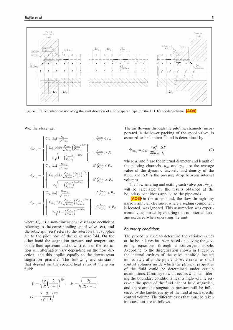
The procedure used to determine the variable valuesat the boundaries has been based on solving the gov-erning equations through a convergent nozzle.According to the discretization shown in Figure 3,the internal cavities of the valve manifold locatedimmediately after the pipe ends were taken as smallcontrol volumes inside which the physical propertiesof the fluid could be determined under certainassumptions. Contrary to what occurs when consider-ing the boundary conditions near a high-volume res-ervoir the speed of the fluid cannot be disregarded,and therefore the stagnation pressure will be influ-enced by the kinetic energy of the fluid at each specificcontrol volume. The different cases that must be takeninto account are as follows.
Figure 3. Computational grid along the axial direction of a non-tapered pipe for the HLL first-order scheme. [AQ9]
Trujillo et al. 5
1. Subsonic inflow
dP
dt
� �p
�%papdu
dt
� �p
¼ ð� � 1Þ% _qþ u4f
Dp
u2
2
u
juj
� �
�a2%u
A
dA
dx�
4f
Dp
%au2
2
u
juj¼ 0
ð10Þ
%TuTAT
AP¼ %PuP ð11Þ
a2C ¼ a2P þð� � 1Þ
2u2P ð12Þ
PC
PT¼
%C%T
� ��ð13Þ
a2C ¼ a2T þð� � 1Þ
2u2T ð14Þ
PT ¼ PP ð15Þ
2. Sonic inflow: in this case the equations governingthe flow are the ones described above with theexception of the last equation, which will bereplaced by the condition aT ¼ uT.
3. Subsonic outflow
Figure 4. (a) Views of the air blowing experimental unit. (b) Schematic drawing of the experimental set-up. [AQ13]
6 Proc IMechE Part C: J Mechanical Engineering Science 0(0)
dP
dt
� �p� %pap
du
dt
� �p
¼ ð� � 1Þ% _qþ u4f
Dp
u2
2
u
juj
� �
�a2%u
A
dA
dx�
4f
Dp
%au2
2
u
juj¼ 0
ð16Þ
%TuTAT
AP¼ %PuP ð17Þ
dP
dt
� �p
� a2Pd%
dt
� �P
¼ ð� � 1Þ% _qþ u4f
Dp
u2
2
u
juj
� �ð18Þ
a2C ¼ a2P þð� � 1Þ
2u2P ð19Þ
PP
PT¼
%P%T
� ��ð20Þ
a2P þð� � 1Þ
2u2P ¼ a2T þ
ð� � 1Þ
2u2T ð21Þ
PT ¼ PC ð22Þ
4. Sonic outflow: similarly to the sonic inflow theequations described above for the subsonic out-flow can be used for the sonic case but with theexception of the last equations which must be sub-stituted by aT ¼ uT. [AQ10]
Therefore the state of gas at each boundary isobtained by solving the above equations coupledwith the wave characteristics.21,22 To determine theboundary condition at the pipe end connected withthe vessel, the state in the vessel at time tþ�t isobtained explicitly from the state at time t.
Experimental set-up
The pneumatic configuration, previously detailed inFigure 1, will now be experimentally reproduced. Themain purpose of the tests will be to assess the pressureand temperature variation at different locations of thesingle station air blowing unit. The high-pressure tankwas supplied with a compressed air bottle charged upto 200 bar, while the low-pressure vessel was providedwith compressed air from the existing line. The unitswere connected to the corresponding ports of the valvemanifold, and similarly the output ports of the valvemanifold were piped to the so-called cavity and recy-cling chambers. As mentioned in previous sections thestatic pressure inside the tanks was measured with pres-sure sensors (range: 0–10 bar, accuracy �0.5% F.S.;range: 0–100 bar, accuracy �2.5% F.S.), while theinstantaneous gas temperature inside each volumewas monitored with self-manufactured K-type thermo-couples with an accuracy of �0.5�C over a measuredrange that goes from 25�C to 100�C. Data-logging as
well as the operating sequence of the pilot valves wasmonitored and programmed with Labview respect-ively. [AQ11] [AQ12]
The operating conditions of the single-stationblowing unit were defined on the basis of the blowingstages applied by the PET manufacturers. The valveopening/closing sequencing arose from systematictesting. The initial trials helped to identify the limita-tions of the first prototypes. The maximum operatingpressure under which the valve manifold was able towork varied between 20 and 30 bar respectively.Based on those results as well as on the limited sizeof the high-pressure tank the blowing test was set upin order to work up to a maximum operating pressureof 25 bar. [AQ14]
Based on the existing concept, the operatingvalve sequence plays a very important role duringthe first stage of the blowing process. The responsetime of the valves must be taken into account whendefining the working cycle. The first experimentalresults helped to understand that the pressure inthe cavity chamber usually exceeded the primary pres-sure when being supplied by the recovery tank.During the low-pressure blowing stage the pressurein the cavity chamber should not overtake theassigned low-pressure level, however, the responsetime of V2 is not fast enough to prevent this type offunctioning. Therefore it is necessary to energize V2
before the pressure level in the cavity chamberreaches the requested value. Due to this fact, apressure peak within the cavity vessel may begenerated during the low-pressure blowing stage,which can be explained by the lack of a regulatingdevice acting between the two vessels, so the internalgeometry of the valve manifold as well as the existingpneumatic connections will constrain the efficiency ofthe system.
The situation described above only occurs if thepressure in the recovery tank at the end of the blowingcycle has reached a designated pressure level. Usuallythis level for the experimental tests under discussion isone and a half times or more the primary pressurePlowð Þ.
Results and discussion
Figures 5 illustrates the pressure characteristics basedon the test set-ups highlighted in blue in Table 2. Theresults demonstrate a fairly clear correlation betweenthe experimental and predicted results when using theMOC as well as the HLL solver in combination withthe Fortran subroutine that solves the set of equationsthat allow measurement of the influence of the valvemanifold. On the contrary, when employing non-dimensional parameters C, bð Þ to estimate the flowrate through the valve manifold ports, the result dif-fers significantly from the empirical values. It must benoted that this approach was exclusively applied incombination with the MOC (MOC0).
Trujillo et al. 7
On the other hand the progressive increase in pres-sure experienced within the recycling vessel, after feed-ing the cavity tank with recycled air, could not bereproduced with any of the solving methods. Even ifthe MOC provides a more realistic prediction, it is stillbelow the maximum experimental recycling ratio thatmay be reached with the different pipe configurations.Moreover, this mathematical method faces some dif-ficulties when referring to the stability of the flow atthe boundaries. In this case the assumptions appliedare not sufficiently consistent since the inner volumewhere the flow charge and discharge is quite small. Onthe contrary, the HLL Riemann solver shows a moreaccurate correlation which may be explained by thefact that the kinetic energy at the boundaries was notdisregarded.
[AQ15]Additionally, when changing the state ofvalve V3 at the end of the recycling phase, the remain-ing air in the cavity is exhausted to the atmosphere.The empirical results show a transition time which hasnot been reproduced by the simulation. As a matter offact this delay was not intentionally generated during
the experimental set-up. The reason behind thisbehaviour is based on the fact that the time requiredto equalize the pressure in the cavity and the recyclingvessel was lower than the set-up time given to switchon valve V3. The mathematical model, however, auto-matically alters the state of valve V3 at the time thatthe pressures in the two tanks become the same. Thisdiscrepancy only affects the cycle time, not the recy-cling ratio.
All the illustrations indicate a promising correl-ation between the empirical and predicted valueswhen observing the results obtained with the HLLsolver model, however, the recycling rate is alwaysbelow the experimental value, which is over 12 bar.In regards to this last aspect, it should be pointed outthat despite the fact that the MOC shows closer cor-respondence with the empirical results, those are stillbelow the previously mentioned pressure level.
Under the assumption that the pneumatic circuitshown in Figure 4 is part of a PET bottle stretchblow moulding machine with a production rate of20,000 bottles per hour (this value being a variable
Figure 5. Pressure characteristics according to Test-1, Test-56, Test-26, and Test-76. HLL: subscript that refers to the HLL Riemann
solver in combination with the valve manifold model; res: subscript that refers to the low- and high-pressure reservoirs respectively;
MOC: subscript that refers to the MOC in combination with the valve manifold model; exp: subscript that refers to the experimental
results; and MOC0: subscript that refers to the MOC in combination with the valve manifold represented by an equivalent elective
orifice area.
8 Proc IMechE Part C: J Mechanical Engineering Science 0(0)
which depends on the blowing machine concept andthe volume of the item to be produced), a pre-blowingphase of 7 bar and a final blowing phase of 23 bar, itmay be determined that the maximum theoretical
energy consumption is 23 � 102 Nm2 �
0:0015�20, 0003600
m3
s ¼ 19:2kW (note that the volume of the mould cavity understudy is 1.5 dm3). The experimental results (refer toFigure 5) demonstrate that up to a minimum pressure
Figure 6. Experimental results according to set-up Test-1 (refer to Table 2).
Trujillo et al. 9
of 12 bar could be ensured at the end of the recyclingphase, which is equivalent to 10 kW. Hence, the effi-ciency of the blowing machine is as follows:
� ¼Energy recovered
Energy supplied¼
10
19:2¼ 0:52 ð23Þ
However, the main drawback of this proposal is thatthe only way to increase the recovery rate is to providea higher pressure level during the secondary phase or,conversely, delay the recovery process until the speci-fic pressure level in the recovery tank is reached. Thislast point can only be accomplished after a certainnumber of operating cycles, in other words, onerecovery cycle will not be enough to reach a certainpressure level and therefore the pneumatic system willbecome less efficient.
Conclusion
The primary intent of this work has been to demonstratethe difficulties of improving the efficiency of a standardhigh-pressure pneumatic application. Specifically, atten-tion has been focused on analysing an air-blowing PETbottle single-station unit. In pursuing this goal, it hasbeen necessary to apply various mathematical methodsin order to learn about the particular aspects of theunsteady flow through the pipes, develop a specialvalve manifold and later manufacturing, and finally,reproduce the industrial operating conditions, takinginto account the existing constraints of our test facility,and monitor the pressure and temperature characteris-tics under different configurations.
[AQ16]The experimental set-up phase was provedto be capable of reproducing the industrial conditionsnormally used by PET bottle manufacturers. The majordrawback, associated with the maximum pressure levelthat could be ensured during the high-pressure air
Table 2. Matrix of test set-ups (dimensions in mm).
10 Proc IMechE Part C: J Mechanical Engineering Science 0(0)
blowing stage, was not an obstacle to validate the func-tionality of the pneumatic system. The pressure historyduring the air-blowing experiments exhibited a cleardependence on the heat transfer through the vesseland pipe walls. As demonstrated, the amount ofrecycled air supplied to the cavity vessel during thelow-pressure air blowing phase allowed avoiding theuse of a low-pressure compressor. It must be noticedthat the air recovery ratio could feed the air blowingline during the low-pressure stage after the first operat-ing cycle. This solution, therefore, ensures a high effi-ciency rate which allowed up to 52% of air recovery;however, it must be kept in mind that in the case ofincreasing the cavity volume (bottle) the recycling linemust also experience a percentage increase in order tobalance the pressure/volume rate between both. Thedesign of a valve manifold including an air recoveryport could be successfully accomplished and revealedthe strong impact on the pressure characteristics overa certain number of operating cycles. From this lastpoint, it can be concluded that the manifold could notbe considered as a flow restriction with an equivalentorifice area since the internal design plays a very import-ant role in the amount of air that can be recovered. Thenumerical models were demonstrated to be in agreementwith the experimental data, especially when coupling theunsteady fluid flow governing equations at the pipes withthe set of equations that rule the pressure and tempera-ture characteristics within the valve manifold.
Acknowledgements
This research was supported by Labson-UPC (ResearchGroup 2014 SGR 575 Generalitat de Catalunya). We
would like to thank Professors Gustavo Raush Alviachand Francisco Javier Freire Venegas, who provided insightand expertise that greatly assisted the research, as well as the
advice given during the revisions of this paper.
Declaration of Conflicting Interests
The author(s) declared no potential conflicts of interest withrespect to the research, authorship, and/or publication of
this article.
Funding
This research received no specific grant from any fundingagency in the public, commercial or not-for-profit sectors.
[AQ17]
References [AQ18] [AQ19]
1. Fukushima H, Handa T and Kodama K. Process for theproduction of blow molded articles accompanied with the
recovery of a blowing gas. Patent 4394333, 1981.2. Wayne C. Recycling of blow air. Patent 4488863, 1984.3. Weiss R. Multiple utilization of working air. Patent
5585066, 1994.
4. Weiss R. Multiple utilization of blow-mold air. Patent5648026, 1994.
5. Siegrist R and Stillhard B. Stretch blow forming method
and blow forming press. Patent WO1996025285 A1,1991.
6. Ikeda M. Air operation method and apparatus of various
20. Andersen B. The analysis and design of pneumatic sys-tems. New York, NY: John Wiley and Sons, Inc, 1967.
21. Lopez E. Methodologies for the numerical simulation of
fluid flow in internal combustion engines. DoctoralDissertation, 2009 [AQ26].
22. Lopez E and Nigro N. Validation of a 0D/1D compu-
tational code for the design of several kind of internalcombustion engines. Investigacion aplicada latinoameri-cana 2010 [AQ27].
Appendix
Notation
Roman symbols
� Heat transfer coefficient Wm2�C
€z Spool valve acceleration ½m
s2�
_q Rate of heat transfer per unit mass of
fluid and per unit time Wkg
h i_z Spool valve velocity ½ms �
_m Mass flow rate ½kgs �� System efficiency� Ratio of specific heat ½��
� Fluid dynamic viscosity kgms
h i% Mass density kg
m3
h iA Area [m2]a Velocity of sound m
s
A0 Orifice area [m2]b Critical pressure ratio [–]C Fluid state at the chamberC Sonic conductance of a component
under test m4�skg
h iCd Discharge coefficient [–]cf Viscous friction damping coefficient for
moving parts in the valve ½kgs �
cp Specific heat at constant pressure Jkg�K
h icv Specific heat at constant volume J
kg�K
h iDp Pipe diameter [m]e0 Stagnation internal energy ½ Jkg�f Friction coefficient in the pipe [–]Fc Friction force on the spool valve [N]Ff Flow forces acting on the spool
valve [N]Fs Static forces acting on the spool
valve [N]g Gravity acceleration m
s2
in Entry fluid flow to the spool valve
control volumek Spring constant N
m
m Fluid mass [kg]ms Mass of moving parts in the valve
manifold [kg]out Exit fluid flow from the spool valve
control volumeP Fluid pressure [Pa]P Fluid state at the pipe endPcr Critical pressure
R Gas constant 287 Jkg�K
h iT Fluid state at the nozzle throatT Gas temperature [�K]t Time [s]Tw Wall temperature [�K]u Gas velocity in x-direction m
s
V Gas volume [m3]v Velocity of jet at vena contracta m
s
vi Index referring to each spool valve of
the valve manifoldw Inner surface of vesselx Cartesian coordinate [m]z Spool valve displacement [m]zo Initial displacement of spool valve [m]
12 Proc IMechE Part C: J Mechanical Engineering Science 0(0)