Proceedings - spars2011.eng.ed.ac.uk€¦ · each community is generally aware of the others’...

4th Workshop on Signal Processing with Adaptive

Sparse Structured Representations

June 27-30, 2011

Edinburgh

Proceedings

11

0

Workshop: Signal Processing with Adaptive Sparse Structured

Representations

June 27-30, 2011

Edinburgh, UK

Cover photo by Oliver-Bonjoch, available under a Creative Commons Attribution-Share Alike 3.0 Unported license.

Foreword

It is with great pleasure that we welcome you to the beautiful city of Edinburgh, the historical home of sampling theory1,for the 4th Workshop on Signal Processing with Adaptive Sparse Structured Representations: SPARS ’11.

Sparse models have already been applied with outstanding success in signal and image processing as well as in machinelearning. In machine learning they provide a powerful method for model order selection within regression and classifica-tion problems (e.g. Lasso). While in signal processing they have led to many algorithms for de-noising, compression (e.g.jpeg2000), de-blurring and more.

In particular, these techniques are at the core of compressed sensing, an emerging approach which proposes a radicallynew viewpoint on signal acquisition compared to Shannon sampling. There are also strong connections between sparsesignal models and kernel methods, whose algorithmic success on large datasets relies deeply on sparsity.

The aim of this workshop is to bring together different work in this area from the applied mathematics, signal processingand machine learning communities. Both theoretical developments and practical applications will be discussed. Althougheach community is generally aware of the others’ work we hope that such a meeting will provide an excellent opportunityfor dialog between the communities.

As with any workshop of this type there is a great deal of work required to make it happen. We would like to take thisopportunity to thank the International Centre for Mathematical Sciences (ICMS) for not only managing the workshopfor us but also for substantially funding it – therefore making the extremely low registration fees possible. We would alsolike to thanks our other sponsors: the UK Engineering and Science Research Council (EPSRC), and the London Math-ematics Society (LMS) for financial assistance; and INRIA Rennes for the use of their website for the abstract submissions.

The other group of people without whom the conference would not happen is our team of PhD students and post-doctoralresearchers at the Edinburgh Centre for Compressed Sensing (E-CoS). Beyond their usual roles in E-CoS they have beenassigned various unenviable tasks to make sure that the workshop runs as smoothly as possible. For this we thank them.

Our final thanks go to our magnificent line up of plenary speakers. Despite high demand we have been able to secure thisworld leading set of speakers from across the globe.

We sincerely hope that everyone will enjoy this workshop and that it will prove to be both enlightening and fun.

Coralia CartisMike DaviesJared Tanner

1E. T. Whittaker, “On the Functions Which are Represented by the Expansions of the Interpolation Theory”, Proc. Royal Soc. Edinburgh,Sec. A, vol.35, pp. 181–194, 1915

2

Committees

OrganisersCoralia Cartis - School of Mathematics, University of Edinburgh, UKMike Davies - School of Engineering & Electronics, University of Edinburgh, UKJared Tanner - School of Mathematics, University of Edinburgh, UK

Steering Committee

Laurent Daudet - Universit Paris Diderot, FranceStephane Canu - INSA de Rouen, FranceMike Davies - University of Edinburgh, UKJalal Fadili - GREYC-ENSICAEN, FranceRemi Gribonval - Centre de Recherche INRIA Rennes,FranceMark Plumbley - Queen Mary University of London, UK

Scott Rickard - UCD CASL & University College Dublin,IrelandJared Tanner - University of Edinburgh, UKBruno Torresani - LATP, CMI, Universite de Provence,FrancePierre Vandergheynst - Ecole Polytechnique Federale deLausanne, Switzerland

Technical Program Committee (abstract referees)

Coralia Cartis - University of Edinburgh, UKLaurent Daudet - Universit Paris Diderot, FranceMike Davies - University of Edinburgh, UKMichael Elad - Technion, IsraelJalal Fadili - GREYC-ENSICAEN, FranceMario Figueiredo - Instituto Superior Tecnico, PortugalRemi Gribonval - Centre de Recherche INRIA Rennes,France

Gabriel Peyre - Universite Paris-Dauphine, FranceJustin Romberg - Georgia Tech, USAJared Tanner - University of Edinburgh, UKBruno Torresani - LATP, CMI, Universite de Provence,FranceJoel Tropp - California Institute of Technology, USA

Edinburgh Compressed Sensing Group

Jared Tanner - University of Edinburgh, UKMike Davies - University of Edinburgh, UKCoralia Cartis - University of Edinburgh, UKPeter Richtarik - University of Edinburgh, UKNatalia Bochkina - University of Edinburgh, UKPaolo Favaro - Heriot-Watt University & University of Ed-inburgh, UKMehrdad Yaghoobi - University of Edinburgh, UKMartin Lotz - University of Edinburgh, UKGabriel Rilling - University of Edinburgh, UKMichael Lexa - University of Edinburgh, UK

Fabien Millioz - University of Edinburgh, UKPavel Zhlobich - University of Edinburgh, UKAndrew Thompson - University of Edinburgh, UKBubacarr Bah - University of Edinburgh, UKKe Wei - University of Edinburgh, UKChunli Guo - University of Edinburgh, UKShaun Kelly - University of Edinburgh, UKMartin Takac - University of Edinburgh, UKJeffrey Blanchard - Grinnell College, USAThomas Blumensath - University of Oxford, UK

3

Technical Program

Monday 27 Tuesday 28 Wednesday 29 Thursday 30

09:00-09:50 Registration Francis Bach David L. Donoho Joel A. Tropp

09:50-10:20 Welcome (10:00) Coffee Break Coffee Break Coffee Break

10:20-11:20 Yi Ma#5 Classification & #11 CS Theory #17 Dictionary Learning

Clustering #12 Sparsity Applications #18 A to D Conversions#6 Structured Sparsity 1

11:20-11:50 Coffee Break Break Break Break

11:50-12:50

#19 Low Dimensional &#1 Sparsity Theory #7 Random Matrix Theory #13 Generalized CS Analysis Sparse Model#2 SAR Imaging #8 Structured Sparsity 2 #14 Estimation & Learning

Detection #20 Performance Evaluations

12:50-14:30 Lunch Lunch Lunch Lunch

14:30-15:20 David J. Brady Remi Gribonval Martin Vetterli Stephen Wright

15:20-16:00 Posters A & Coffee Posters A & Coffee Posters B & Coffee Posters B & Coffee

16:00-17:00

#15 Generalized#3 Medical Imaging #9 Analysis Framework Sampling Techniques #21 PCA/ICA/BSS#4 Sparse Approx. & #10 Dynamical & #16 Sparse Approx. & #22 Sparse Filter Design

CS Algorithms 1 Time-varying Systems CS Algorithms 2

Evening WineReception, Whisky Tasting Excursion,

(18:00-21:00) £20 cost(18:30-22:00)

Note: Plenary talks and sessions with odd numbers take place in the “Main Auditorium” (in the QueenMother Conference Centre) and sessions with even numbers take place in the “Great Hall”.

4

Abstracts

Plenary Talks: Monday 2710:20-11:20

TILT and RASL: For Low-Rank Structures in Images and DataYi Ma . . . . . . . . . . . . . . . . . . . . . . . . . . . . . . . . . . . . . . . . . . . . . . . . 10

14:30-15:20Coding for Multiplex Optical Imaging

David J. Brady . . . . . . . . . . . . . . . . . . . . . . . . . . . . . . . . . . . . . . . . . . . 12

Plenary Talks: Tuesday 2809:00-09:50

Strutured Sparsity-Inducing Norms through Submodular FunctionsFrancis Bach . . . . . . . . . . . . . . . . . . . . . . . . . . . . . . . . . . . . . . . . . . . . 13

14:30-15:20Sparsity & Co.: An Overview of Analysis vs Synthesis in Low-Dimensional Signal Models

Remi Gribonval . . . . . . . . . . . . . . . . . . . . . . . . . . . . . . . . . . . . . . . . . . 14

Plenary Talks: Wednesday 2909:00-09:50

Precise Optimality Results in Compressed SensingDavid L. Donoho . . . . . . . . . . . . . . . . . . . . . . . . . . . . . . . . . . . . . . . . . . 15

14:30-15:20Sampling in the Age of Sparsity

Martin Vetterli . . . . . . . . . . . . . . . . . . . . . . . . . . . . . . . . . . . . . . . . . . . 16

Plenary Talks: Thursday 3009:00-09:50

Finding structure with randomnessJoel A. Tropp . . . . . . . . . . . . . . . . . . . . . . . . . . . . . . . . . . . . . . . . . . . 17

14:30-15:20Gradient Algorithms for Regularized Optimization

Stephen Wright . . . . . . . . . . . . . . . . . . . . . . . . . . . . . . . . . . . . . . . . . . 18

Contributed Talks: Monday 27#1 Sparsity Theory (11:50-12:50)

Optimally Sparse FramesPeter Casazza, Andreas Heinecke, Felix Krahmer, Gitta Kutyniok . . . . . . . . . . . . . . 19

Lagrangian Biduality of the `0- and `1-Minimization ProblemsDheeraj Singaraju, Allen Yang, Shankar Sastry, Roberto Tron, Ehsan Elhamifar . . . . . . 20

Signal Recovery Via `p Minimization: Analysis using Restricted Isometry PropertyShisheng Huang, Jubo Zhu, Fengxia Yan, Meihua Xie, Zelong Wang . . . . . . . . . . . . . 21

#2 SAR Imaging (11:50-12:50)Compressed sensing for joint ground imaging and target indication with airborne radar

Ludger Prunte . . . . . . . . . . . . . . . . . . . . . . . . . . . . . . . . . . . . . . . . . . . 22Automatic target recognition from highly incomplete SAR data

Chaoran Du, Gabriel Rilling, Mike Davies, Bernard Mulgrew . . . . . . . . . . . . . . . . . 23

5

Tomographic SAR Inversion via Sparse ReconstructionXiao Xiang Zhu, Richard Bamler . . . . . . . . . . . . . . . . . . . . . . . . . . . . . . . . . 24

#3 Medical Imaging (16:00-17:00)On the efficiency of proximal methods for CBCT and PET reconstruction with sparsity constraint

Sandrine Anthoine, Jean-Francois Aujol, Yannick Boursier, Melot Clothilde . . . . . . . . . 25Reliable Small-object Reconstruction from Sparse Views in X-ray Computed Tomography

Jakob Heide Joergensen, Emil Y. Sidky, Xiaochuan Pan . . . . . . . . . . . . . . . . . . . . 26Near-optimal undersampling and reconstruction for MRI carotid blood flow measurement based on

support splittingGabriel Rilling, Yuehui Tao, Mike E. Davies, Ian Marshall . . . . . . . . . . . . . . . . . . 27

#4 Sparse Approximation and Compressed Sensing Algorithms 1 (16:00-17:00)Denoising signal represented by mixtures of multivariate Gaussians in a time-frequency dictionary

Emilie Villaron, Sandrine Anthoine, Bruno Torresani . . . . . . . . . . . . . . . . . . . . . 28Efficiency of Randomized Coordinate Descent Methods on Minimization Problems with a Composite

Objective FunctionMartin Takac, Peter Richtarik . . . . . . . . . . . . . . . . . . . . . . . . . . . . . . . . . . 29

Robust sparse recovery with non-negativity constraintsMartin Slawski, Matthias Hein . . . . . . . . . . . . . . . . . . . . . . . . . . . . . . . . . . 30

Contributed Talks: Tuesday 28#5 Classification and Clustering (10:20-11:20)

Sparse Subspace ClusteringEhsan Elhamifar, Rene Vidal . . . . . . . . . . . . . . . . . . . . . . . . . . . . . . . . . . . 31

Subspace Clustering by Rank MinimizationPaolo Favaro, Avinash Ravichandran, Rene Vidal . . . . . . . . . . . . . . . . . . . . . . . 32

Multiscale Geometric Dictionaries for Point-cloud DataGuangliang Chen, Mauro Maggioni . . . . . . . . . . . . . . . . . . . . . . . . . . . . . . . 33

#6 Structured Sparsity 1 (10:20-11:20)Modeling Statistical Dependencies in Sparse Representations

Tomer Faktor, Yonina C. Eldar, Michael Elad . . . . . . . . . . . . . . . . . . . . . . . . . 34A source localization approach based on structured sparsity for broadband far-field sources

Aris Gretsistas, Mark Plumbley . . . . . . . . . . . . . . . . . . . . . . . . . . . . . . . . . 35Sparsity with sign-coherent groups of variables via the cooperative-Lasso

Julien Chiquet, Yves Grandvalet, Camille Charbonnier . . . . . . . . . . . . . . . . . . . . 36

#7 Random Matrix Theory (11:50-12:50)Tail bounds for all eigenvalues of a sum of random matrices

Alex Gittens, Joel Tropp . . . . . . . . . . . . . . . . . . . . . . . . . . . . . . . . . . . . . 37Random Projections are Nearly Isometric For Parametric Functions Too

William Mantzel, Justin Romberg . . . . . . . . . . . . . . . . . . . . . . . . . . . . . . . . 38Concentration Inequalities and Isometry Properties for Compressive Block Diagonal Matrices

Han Lun Yap, Jae Young Park, Armin Eftekhari, Christopher Rozell, Michael Wakin . . . 39

#8 Structured Sparsity 2 (11:50-12:50)Sparse Anisotropic Triangulations and Image Estimation

Laurent Demaret . . . . . . . . . . . . . . . . . . . . . . . . . . . . . . . . . . . . . . . . . . 40Compressive Sensing with Biorthogonal Wavelets via Structured Sparsity

Marco Duarte, Richard Baraniuk . . . . . . . . . . . . . . . . . . . . . . . . . . . . . . . . . 41A convex approach for structured wavelet sparsity patterns

Nikhil Rao, Robert Nowak, Stephen Wright, Nick Kingsbury . . . . . . . . . . . . . . . . . 42

#9 Analysis Framework (16:00-17:00)Hybrid Synthesis-Analysis Frame-Based Regularization: A Criterion and an Algorithm

Manya Afonso, Jose Bioucas-Dias, Mario Figueiredo . . . . . . . . . . . . . . . . . . . . . . 43Cosparse Analysis Modeling

Sangnam Nam, Michael E. Davies, Michael Elad, Remi Gribonval . . . . . . . . . . . . . . 44

6

Implications for compressed sensing of a new sampling theorem on the sphereJason McEwen, Gilles Puy, Jean-Philippe Thiran, Pierre Vandergheynst, Dimitri Van DeVille . . . . . . . . . . . . . . . . . . . . . . . . . . . . . . . . . . . . . . . . . . . . . . . . . 45

#10 Dynamical and Time-varying Systems (16:00-17:00)Compressive Sensing for Gaussian Dynamic Signals

Wei Dai, Dino Sejdinovic, Olgica Milenkovic . . . . . . . . . . . . . . . . . . . . . . . . . . 46Simultaneous Estimation of Sparse Signals and Systems at Sub-Nyquist Rates

Hojjat Akhondi Asl, Pier Luigi Dragotti . . . . . . . . . . . . . . . . . . . . . . . . . . . . . 47A Hierarchical Re-weighted-`1 Approach for Dynamic Sparse Signal Estimation

Adam Charles, Christopher Rozell . . . . . . . . . . . . . . . . . . . . . . . . . . . . . . . . 48

Contributed Talks: Wednesday 29#11 Compressed Sensing Theory (10:20-11:20)

Weighted Lp Constraints in Noisy Compressed SensingLaurent Jacques, David Hammond, Jalal Fadili . . . . . . . . . . . . . . . . . . . . . . . . . 49

Spread Spectrum for Universal Compressive SamplingGilles Puy, Pierre Vandergheynst, Remi Gribonval, Yves Wiaux . . . . . . . . . . . . . . . 50

On Bounds of Restricted Isometry Constants for Gaussian Random MatricesBubacarr Bah, Jared Tanner . . . . . . . . . . . . . . . . . . . . . . . . . . . . . . . . . . . 51

#12 Sparsity Applications (10:20-11:20)Towards Optimal Data Acquisition in Diffuse Optical Tomography: Analysis of Illumination Patterns

Marta Betcke, Simon Arridge . . . . . . . . . . . . . . . . . . . . . . . . . . . . . . . . . . . 52Recent evidence of sparse coding in neural systems

Christopher Rozell, Mengchen Zhu . . . . . . . . . . . . . . . . . . . . . . . . . . . . . . . . 53Sparse Detection in the Chirplet Transform

Fabien Millioz, Mike Davies . . . . . . . . . . . . . . . . . . . . . . . . . . . . . . . . . . . . 54

#13 Generalized Compressed Sensing (11:50-12:50)Riemannian optimization for rank minimization problems

Bart Vandereycken . . . . . . . . . . . . . . . . . . . . . . . . . . . . . . . . . . . . . . . . . 55The degrees of freedom of the Lasso in underdetermined linear regression models

Maher Kachour, Jalal Fadili, Christophe Chesneau, Charles Dossal, Gabriel Peyre . . . . . 56Guaranteed recovery of a low-rank and joint-sparse matrix from incomplete and noisy measurements

Mohammad Golbabaee, Pierre Vandergheynst . . . . . . . . . . . . . . . . . . . . . . . . . 57

#14 Estimation and Detection (11:50-12:50)Message-Passing Estimation from Quantized Samples

Ulugbek Kamilov, Vivek Goyal, Sundeep Rangan . . . . . . . . . . . . . . . . . . . . . . . 58Ambiguity Sparse Processes

Sofia Olhede . . . . . . . . . . . . . . . . . . . . . . . . . . . . . . . . . . . . . . . . . . . . 59Sparseness-based non-parametric detection and estimation of random signals in noise

Dominique Pasto, Abdourrahmane Atto . . . . . . . . . . . . . . . . . . . . . . . . . . . . . 60

#15 Generalized Sampling Techniques (16:00-17:00)Reconstruction and Cancellation of Sampled Multiband Signals Using Discrete Prolate Spheroidal

SequencesMark Davenport, Michael Wakin . . . . . . . . . . . . . . . . . . . . . . . . . . . . . . . . . 61

Exponential Reproducing Kernels for Sparse SamplingJose Antonio Uriguen, Pier Luigi Dragotti, Thierry Blu . . . . . . . . . . . . . . . . . . . . 62

Generalized sampling and infinite-dimensional compressed sensingAnders Hansen, Ben Adcock . . . . . . . . . . . . . . . . . . . . . . . . . . . . . . . . . . . 63

#16 Sparse Approximation and Compressed Sensing Algorithms 2 (16:00-17:00)A Lower Complexity Bound for `1-regularized Least-squares Problems using a Certain Class of Al-

gorithmsTobias Lindstrøm Jensen . . . . . . . . . . . . . . . . . . . . . . . . . . . . . . . . . . . . . 64

A New Recovery Analysis of Iterative Hard Thresholding for Compressed SensingAndrew Thompson, Coralia Cartis . . . . . . . . . . . . . . . . . . . . . . . . . . . . . . . . 65

7

Recipes for Hard Thresholding MethodsAnastasios Kyrillidis, Volkan Cevher . . . . . . . . . . . . . . . . . . . . . . . . . . . . . . . 66

Contributed Talks: Thursday 30#17 Dictionary Learning (10:20-11:20)

Local optimality of dictionary learning algorithmsBoris Mailhe, Mark Plumbley . . . . . . . . . . . . . . . . . . . . . . . . . . . . . . . . . . . 67

Approximate Message Passing for Bilinear ModelsPhilip Schniter, Volkan Cevher . . . . . . . . . . . . . . . . . . . . . . . . . . . . . . . . . . 68

Structure-Aware Non-Negative Dictionary LearningKen O’Hanlon, Mark Plumbley . . . . . . . . . . . . . . . . . . . . . . . . . . . . . . . . . . 69

#18 Analogue to Digital Conversions (10:20-11:20)Multi-Channel Analog-to-Digital (A/D) Conversion using Fewer A/D Converters than Channels

Ahmed H. Tewfik, Youngchun Kim, B. Vikrham Gowreesunker . . . . . . . . . . . . . . . . 70Practical Design of a Random Demodulation Sub-Nyquist ADC

Stephen Becker, Juhwan Yoo, Mathew Loh, Azita Emami-Neyestanak, Emmanuel Candes . 71Compressive Spectral Estimation Can Lead to Improved Resolution/Complexity Tradeoffs

Michael Lexa, Mike Davies, John Thompson . . . . . . . . . . . . . . . . . . . . . . . . . . 72

#19 Low Dimensional and Analysis Sparse Model Learning (11:50-12:50)K-SVD Dictionary-Learning for Analysis Sparse Models

Ron Rubinstein, Michael Elad . . . . . . . . . . . . . . . . . . . . . . . . . . . . . . . . . . 73Analysis Operator Learning for Overcomplete Cosparse Representations

Mehrdad Yaghoobi, Sangnam Nam, Remi Gribonval, Mike E. Davies . . . . . . . . . . . . 74Learning hybrid linear models via sparse recovery

Eva Dyer, Aswin Sankaranarayanan, Richard Baraniuk . . . . . . . . . . . . . . . . . . . . 75

#20 Performance Evaluations (11:50-12:50)Evaluating Dictionary Learning for Sparse Representation Algorithms using SMALLbox

Ivan Damnjanovic, Matthew Davies, Mark Plumbley . . . . . . . . . . . . . . . . . . . . . . 76A Reproducible Research Framework for Audio Inpainting

Amir Adler, Valentin Emiya, Maria G. Jafari, Michael Elad, Remi Gribonval . . . . . . . . 77GPU Accelerated Greedy Algorithms for Sparse Approximation

Jeffrey Blanchard, Jared Tanner . . . . . . . . . . . . . . . . . . . . . . . . . . . . . . . . . 78

#21 PCA/ICA/BSS (16:00-17:00)Two Proposals for Robust PCA Using Semidefinite Programming

Michael McCoy, Joel Tropp . . . . . . . . . . . . . . . . . . . . . . . . . . . . . . . . . . . . 79Blind Source Separation of Compressively Sensed Signals

Martin Kleinsteuber, Hao Shen . . . . . . . . . . . . . . . . . . . . . . . . . . . . . . . . . . 80Finding Sparse Approximations to Extreme Eigenvectors: Generalized Power Method for Sparse

PCA and ExtensionsPeter Richtarik, Michel Journee, Yurii Nesterov, Rodolphe Sepulchre . . . . . . . . . . . . 81

#22 Sparse Filter Design (16:00-17:00)Stable Embeddings of Time Series Data

Han Lun Yap, Christopher Rozell . . . . . . . . . . . . . . . . . . . . . . . . . . . . . . . . 82Estimating multiple filters from stereo mixtures: a double sparsity approach

Simon Arberet, Prasad Sudhakar, Remi Gribonval . . . . . . . . . . . . . . . . . . . . . . . 83Well-posedness of the frequency permutation problem in sparse filter estimation with lp minimization

Alexis Benichoux, Prasad Sudhakar, Remi Gribonval . . . . . . . . . . . . . . . . . . . . . 84

Posters AOptical wave field reconstruction based on nonlocal transform-domain sparse regularization for phase

and amplitudeVladimir Katkovnik, Jaakko Astola . . . . . . . . . . . . . . . . . . . . . . . . . . . . . . . 85

Efficient sparse representation based classification using hierarchically structured dictionariesJort Gemmeke . . . . . . . . . . . . . . . . . . . . . . . . . . . . . . . . . . . . . . . . . . . 86

8

Sparse Object-Based Audio Coding Using Non-Negative Matrix Factorization of SpikegramsRamin Picheva, Hossein Najaf-Zadeh, Frederic Mustiere, Christopher Srinivasa, HassanLahdili . . . . . . . . . . . . . . . . . . . . . . . . . . . . . . . . . . . . . . . . . . . . . . . 87

Recovery of Compressively Sampled Sparse Signals using Cyclic Matching PursuitBob Sturm, Mads Christensen . . . . . . . . . . . . . . . . . . . . . . . . . . . . . . . . . . 88

Structured and soft ! Boltzmann machine and mean-field approximation for structured sparse repre-sentationsAngelique Dremeau, Laurent Daudet . . . . . . . . . . . . . . . . . . . . . . . . . . . . . . 89

BM3D-frame sparse image modeling and decoupling of inverse and denoising for image deblurringAram Danielyan, Vladimir Katkovnik, Karen Egiazarian . . . . . . . . . . . . . . . . . . . 90

Super-resolution and reconstruction of far-field ghost imaging via sparsity constraintsWenlin Gong, Shensheng Han . . . . . . . . . . . . . . . . . . . . . . . . . . . . . . . . . . 91

Fast compressive terahertz imagingHao Shen, Lu Gan, Nathan Newman, Yaochun Shen . . . . . . . . . . . . . . . . . . . . . . 92

Dictionary Learning:Application to ECG DenoisingAnastasia Zakharova, Olivier Laligant, Christophe Stolz . . . . . . . . . . . . . . . . . . . . 93

Unsupervised Learning of View-Condition Invariant Sparse Representation for Image Category Clas-sificationHui Ka Yu . . . . . . . . . . . . . . . . . . . . . . . . . . . . . . . . . . . . . . . . . . . . . 94

Joint localisation and identification of acoustical sources with structured-sparsity priorsGilles Chardon, Laurent Daudet . . . . . . . . . . . . . . . . . . . . . . . . . . . . . . . . . 95

An Alternating Direction Algorithm for (Overlapping) Group RegularizationMario Figueiredo, Jose Bioucas-Dias . . . . . . . . . . . . . . . . . . . . . . . . . . . . . . . 96

Sparse Approximation of the Neonatal EEGVladimir Matic, Maarten De Vos, Bogdan Mijovic, Sabine Van Huffel . . . . . . . . . . . . 97

Inversion of 2-D images to estimate densities in R3

Dalia Chakrabarty, Fabio Rigat . . . . . . . . . . . . . . . . . . . . . . . . . . . . . . . . . 98Constrained Non-Negative Matrix Factorization for source separation in Raman Spectroscopy

Herald Rabeson . . . . . . . . . . . . . . . . . . . . . . . . . . . . . . . . . . . . . . . . . . 99Sparse Templates-Based Shape Representation for Image Segmentation

Stefania Petra, Dirk Breitenreicher, Jan Lellmann, Christoph Schnorr . . . . . . . . . . . . 100Wyner-Ziv Coding for Distributed Compressive Sensing

Kezhi Li, Su Gao, Cong Ling, Lu Gan . . . . . . . . . . . . . . . . . . . . . . . . . . . . . . 101Methods for Training Adaptive Dictionary in Underdetermined Speech Separation

Tao Xu, Wenwu Wang . . . . . . . . . . . . . . . . . . . . . . . . . . . . . . . . . . . . . . 102Analysis of Subsampled Circulant Matrices for Imaging

Matthew Turner, Lina Xu, Wotao Yin, Kevin Kelly . . . . . . . . . . . . . . . . . . . . . . 103A new BCI Classification Method based on EEG Sparse Representation

Younghak Shin, Seungchan Lee, Heung-No Lee . . . . . . . . . . . . . . . . . . . . . . . . . 104A Realistic Distributed Compressive Sensing Framework for Multiple Wireless Sensor Networks

Oliver James, Heung-No Lee . . . . . . . . . . . . . . . . . . . . . . . . . . . . . . . . . . . 105

Posters BSparse Phase Retrieval

Shiro Ikeda, Hidetoshi Kono . . . . . . . . . . . . . . . . . . . . . . . . . . . . . . . . . . . 106Probabilistic models which enforce sparsity

Ali Mohammad-Djafari . . . . . . . . . . . . . . . . . . . . . . . . . . . . . . . . . . . . . . 107Greedy Algorithms for Sparse Total Least Squares

Bogdan Dumitrescu . . . . . . . . . . . . . . . . . . . . . . . . . . . . . . . . . . . . . . . . 108Super-resolution based on Sparsity Priori

Hui Wang, Shensheng Han, Mikhail I. Kolobov . . . . . . . . . . . . . . . . . . . . . . . . . 109Fast Compressive Sensing Recovery with Transform-based Sampling

Hung-Wei Chen, Chun-Shien Lu, Soo-Chang Pei . . . . . . . . . . . . . . . . . . . . . . . . 110Feature Selection in Carotid Artery Segmentation Process based on Learning Machines

Rosa-Marıa Menchon-Lar, Consuelo Bastida-Jumilla, Juan Morales Sanchez, Jose-LuisSancho-Gomez . . . . . . . . . . . . . . . . . . . . . . . . . . . . . . . . . . . . . . . . . . . 111

9

Best Basis Matching PursuitTianyao Huang, Yimin Liu, Huadong Meng, Xiqin Wang . . . . . . . . . . . . . . . . . . . 112

Adaptive Algorithm for Online Identification and Recovering of Jointly Sparse SignalsRoi Amel, Arie Feuer . . . . . . . . . . . . . . . . . . . . . . . . . . . . . . . . . . . . . . . 113

Primal-Dual TV Reconstruction in Refractive DeflectometryAdriana Gonzalez, Laurent Jacques, Emmanuel Foumouo, Philippe Antoine . . . . . . . . . 114

Greedy decompositions with randomly varying time-frequency subdictionariesManuel Moussallam, Gael Richard, Laurent Daudet . . . . . . . . . . . . . . . . . . . . . . 115

A Sparsity based Regularization Algorithm with Automatic Parameter EstimationDamiana Lazzaro . . . . . . . . . . . . . . . . . . . . . . . . . . . . . . . . . . . . . . . . . 116

An unsupervised iterative shrinkage/thresholding algorithm for sparse expansion in a union of dic-tionnaries.Matthieu Kowalski, Thomas Rodet . . . . . . . . . . . . . . . . . . . . . . . . . . . . . . . 117

An Infeasible-Point Subgradient Algorithm and a Computational Solver Comparison for `1-MinimizationAndreas Tillmann, Dirk Lorenz, Marc Pfetsch . . . . . . . . . . . . . . . . . . . . . . . . . 118

On the relation between perceptrons and non-negative matrix factorizationHugo Van hamme . . . . . . . . . . . . . . . . . . . . . . . . . . . . . . . . . . . . . . . . . 119

Recovery of finite alphabet signals from incomplete measurementsSi Mohamed Aziz Sbaı, Abdeldjalil Aıssa-El-Bey, Dominique Pastor . . . . . . . . . . . . . 120

Adding Dynamic Smoothing to Mixture Mosaicing SynthesisGraham Coleman, Jordi Bonada, Esteban Maestre . . . . . . . . . . . . . . . . . . . . . . . 121

Block-Sparse Recovery via Convex OptimizationEhsan Elhamifar, Rene Vidal . . . . . . . . . . . . . . . . . . . . . . . . . . . . . . . . . . . 122

Performance limits of the measurements on Compressive Sensing for Multiple Sensor SystemSangjun Park, Hwanchol Jang, Heung-No Lee . . . . . . . . . . . . . . . . . . . . . . . . . 123

Message Passing Aided Least Square Recovery for Compressive SensingJaewook Kang, Heung-No Lee, Kiseon Kim . . . . . . . . . . . . . . . . . . . . . . . . . . . 124

Matrix-free Interior Point Method for Compressed Sensing ProblemsKimonas Fountoulakis, Jacek Gondzio . . . . . . . . . . . . . . . . . . . . . . . . . . . . . . 125

A Block-Based Approach to Adaptively Bias the Weights of Adaptive FiltersLuis Azpicueta-Ruiz, Jeronimo Arenas-Garcıa . . . . . . . . . . . . . . . . . . . . . . . . . 126

10

TILT and RASL: For Low-Rank Structures in Images and DataYi Ma

ECE Department, UIUC and VC Group, Microsoft Research Asia

Abstract—In this talk, we will introduce two fundamental compu-tational tools, namely TILT and RASL, for extracting rich low-rankstructures in images and videos, respectively. Both tools utilize the sametransformed Robust PCA model for the visual data:

D τ = A + E (1)

and use practically the same algorithm for extracting the low-rankstructures A from the visual data D, despite image domain transforma-tion τ and sparse corruptions E. We will show how these two seeminglysimple tools can help unleash tremendous information in images andvideos that we used to struggle to get. We believe these new tools willbring disruptive changes to many challenging tasks in computer visionand image processing, including feature extraction, image correspondenceor alignment, 3D reconstruction, and object recognition, etc.

Y i Ma is the research manager of the Visual Computing group at MicrosoftResearch Asia in Beijing since January 2009. He is also an associate professorat the Electrical & Computer Engineering Department of the University ofIllinois at Urbana-Champaign. His main research interest is in computervision, high-dimensional data analysis, and systems theory. He is the firstauthor of the popular vision textbook “An Invitation to 3-D Vision,” publishedby Springer in 2003. Yi Ma received two Bachelors degree in Automation andApplied Mathematics from Tsinghua University (Beijing, China) in 1995,a Master of Science degree in EECS in 1997, a Master of Arts degree inMathematics in 2000, and a PhD degree in EECS in 2000, all from theUniversity of California at Berkeley. Yi Ma received the David Marr BestPaper Prize at the International Conference on Computer Vision 1999, theLonguet-Higgins Best Paper Prize at the European Conference on ComputerVision 2004, and the Sang Uk Lee Best Student Paper Award with his studentsat the Asian Conference on Computer Vision in 2009. He also received theCAREER Award from the National Science Foundation in 2004 and theYoung Investigator Award from the Office of Naval Research in 2005. Heis an associate editor of IEEE Transactions on Pattern Analysis and MachineIntelligence (PAMI) and the International Journal of Computer Vision (IJCV).He has served as the chief guest editor for special issues for the Proceedingsof IEEE and the IEEE Signal Processing Magazine. He will also serve asProgram Chair for ICCV 2013 in Sydney, Australia. He is a senior memberof IEEE and a member of ACM, SIAM, and ASEE.

This is joint work with John Wright of Columbia, Emmanuel Candes ofStanford, and my students Zhengdong Zhang, Xiao Liang, Yigang Peng ofTsinghua, Arvind Ganesh of UIUC.

11

Coding for Multiplex Optical Imaging

David J. BradyDuke Imaging and Spectroscopy Program, Department of Electrical and Computer Engineering

Duke University, Durham, North Carolina 20291-0291www.disp.duke.edu

Abstract—Efficient sampling of sparse signals requires measurementof linear feature projections. “Weighing design” consists of selectingprojection coefficients to satisfy mathematical and physical objectives.This paper reviews the weighing design problem for applications inspectral imaging, focal tomography and holography.

I. I NTRODUCTION

We consider linear measurement systems described by the forwardmodel g = Hf + n where g is measurement data,H is themeasurement operator,f is the object state andn is noise. The goalof these systems is to estimate, e.g. to image,f giveng. If H is notthe identity operator then the system takes “multiplex measurements”While radar and computed tomography aficinados may considerthemultiplex designation redundant, from 1840 until 1950 imager designemphasized physical design for focal transformations. Theadvent ofdigital computers and electronic detectors changed this goal, but evenafter 60 years the ensuing revolution is still evolving. Compressedsensing theory focuses particular attention on Shannon’s work atthe start of this revolution. This paper considers the implications ofcompressed sensing on two results in measurement theory from thesame era, specifically multiplex spectroscopy [1] and holography [2].

II. SPECTROSCOPY ANDSPECTRAL IMAGING

For over half a century, weighing design for multiplex spectroscopyfocused on linear estimators off given g. While Harwit and Sloanacknowledge in the seminal work on this approach [3] that biasedestimators may achieve better results, very little work on coding fornonlinear estimators appeared before 2000. An important exceptionappears in work on computed tomographic imaging spectrometers,which applied convex optimization to multiplex spectral imaging [4].The goal of this work was to overcome a “missing cone” Radonprojections. More recently, my group has shown that Golay-stylecoded apertures eliminate the missing cone and that compressedsensing theory may be applied to estimate full 3D data cubes fromcoded 2D snapshots [5].

While it is clear that significant advantages arise from the combina-tion of coded projections and constrained optimization, optimal codesfor these systems are currently unknown. This is in sharp contrastto previous theory for linear estimators, which showed Hadamardcodes to be optimal for additive noise and identity operators to beoptimal for Poisson noise. As my talk describes using both simulatedand experimental data, pseudo-random codes may outperformidentityand Hadamard codes when combined with modern regularization andoptmization strategies.

III. F OCAL TOMOGRAPHY

Major practical successes in compressed sensing have arisen inapplications where it is physically impossible to implement H asidentity matrix. Spectral imaging is one such example, others arisein various multidimensional tomographies. Natural imaging of 3Dscenes is tomographic problem of particular interest. Historically,focal imaging systems are map 2D object planes to 2D image planes.

This model has been preferred because focal recording devices (e.g.film and detector arrays) are confined to 2D surfaces. With theadventof computational imaging, however, the physical structureof themeasurement system need not be tied to the physical structure ofthe image. Specifically, one should be able to implement multiplexcodes that enable direct estimation of 3D objects from snapshot data.While adhoc tomographic recording strategies using cameraarraysor pupil coding strategies have been attempted to achieve this goal,systematic studies of codes for native 3D optical imaging are justbeginning. Image space coding strategies similar to those used incoded aperture spectral imaging are particularly attractive for thischallenge.

IV. H OLOGRAPHY

Optical imaging inherently combines analog signal processing inoptical elements with digital image formation. Quasi-focal designwith compact kernel support is essential to reasonable rankmeasure-ment on natural fields. Imagers using laser illumination, incontrast,may achieve reasonable rank measurement operators with unboundedsampling kernels. This allows lensless imaging over large apertures.Unfortunaely, natural objects reflect laser light diffusely, meaning thata random phase is added to the reflected field in each image pixel.Such specular images are not sparse on any basis. This difficultymay be overcome by estimating the magnitude of the scattering crosssection of each pixel, which forms a compressible image. Under thisapproach one seeks to invert transformed statistics of measurementdata to estimate a particular set of object statistics [6]. Weighingdesign for this application consists of selecting both the raw samplingstructure and the synthetic statistics taken as intermediate indicatorsof the object state. Coding for this application introducesnewchallenges and opportunities and suggests novel statistical definitionsfor the concept of compressive sampling.

REFERENCES

[1] M. Golay, “Multislit spectroscopy,”J. Opt. Soc. Amer., vol. 39, pp. 437–444, 1949.

[2] D. Gabor, “A new microscopic principle,”Nature, vol. 161, pp. 777–778,1948.

[3] M. Harwit and N. J. A. Sloane,Hadamard transform optics. AcademicPress, 1979.

[4] A. K. Brodzik and J. M. Mooney, “Convex projections algorithm forrestoration of limited-angle chromotomographic images,”J. Opt. Soc. Am.A, vol. 16, no. 2, pp. 246–257, 1999.

[5] M. E. Gehm, R. John, D. J. Brady, R. M. Willett, and T. J. Schulz, “Single-shot compressive spectral imaging with a dual-disperser architecture,”Opt. Express, vol. 15, no. 21, pp. 14 013–14 027, 2007.

[6] K. Choi, R. Horisaki, J. Hahn, S. Lim, D. L. Marks, T. J. Schulz, andD. J. Brady, “Compressive holography of diffuse objects,”Appl. Opt.,vol. 49, no. 34, pp. H1–H10, Dec 2010.

12

Strutured Sparsity-Inducing Normsthrough Submodular Functions

Francis BachINRIA - Ecole Normale Superieure

Paris, France

Abstract—Sparse methods for supervised learning aim at finding goodlinear predictors from as few variables as possible, i.e., with smallcardinality of their supports. This combinatorial selection problem isoften turned into a convex optimization problem by replacing thecardinality function by its convex envelope (tightest convex lower bound),in this case theℓ1-norm. In this work, we investigate more general set-functions than the cardinality, that may incorporate prior knowledgeor structural constraints which are common in many applications:namely, we show that for nondecreasing submodular set-functions, thecorresponding convex envelope can be obtained from its Lovasz extension,a common tool in submodular analysis. This defines a family ofpolyhedralnorms, for which we provide generic algorithmic tools (subgradientsand proximal operators) and theoretical results (conditions for supportrecovery or high-dimensional inference). By selecting specific submodularfunctions, we can give a new interpretation to known norms, such as thosebased on rank-statistics or grouped norms with potentiallyoverlappinggroups; we also define new norms, in particular ones that can be usedas non-factorial priors for supervised learning.

The concept of parsimony is central in many scientific domains.In the context of statistics, signal processing or machine learning,it takes the form of variable or feature selection problems,and iscommonly used in two situations: First, to make the model or theprediction more interpretable or cheaper to use, i.e., evenif theunderlying problem does not admit sparse solutions, one looks forthe best sparse approximation. Second, sparsity can also beusedgiven prior knowledge that the model should be sparse. In these twosituations, reducing parsimony to finding models with low cardinalityturns out to be limiting, and structured parsimony has emerged as afruitful practical extension, with applications to image processing,text processing or bioinformatics (see, e.g., [1], [2], [3], [4], [5],[6], [7]). For example, in [4], structured sparsity is used to encodeprior knowledge regarding network relationship between genes, whilein [6], it is used as an alternative to structured non-parametricBayesian process based priors for topic models.

Most of the work based on convex optimization and the design ofdedicated sparsity-inducing norms has focused mainly on the specificallowed set of sparsity patterns [1], [2], [4], [6]: ifw ∈ R

p denotesthe predictor we aim to estimate, andSupp(w) denotes its support,then these norms are designed so that penalizing with these normsonly leads to supports from a given family of allowed patterns. Inthis paper, we instead follow the approach of [8], [3] and considerspecific penalty functionsF (Supp(w)) of the support set, which gobeyond the cardinality function, but are not limited or designed toonly forbid certain sparsity patterns. These may also lead to restrictedsets of supports but their interpretation in terms of anexplicit penaltyon the support leads to additional insights into the behavior ofstructured sparsity-inducing norms. While direct greedy approaches(i.e., forward selection) to the problem are considered in [8], [3], weprovide convex relaxations to the functionw 7→ F (Supp(w)), whichextend the traditional link between theℓ1-norm and the cardinality

function.This is done for a particular ensemble of set-functionsF , namely

nondecreasing submodular functions. Submodular functions may beseen as the set-function equivalent of convex functions, and exhibitmany interesting properties—see [9] for a tutorial on submodularanalysis and [10], [11] for other applications to machine learning. Inthis presentation, we will present the following contributions:

−We make explicit links between submodularity and sparsity byshowing that the convex envelope of the functionw 7→ F (Supp(w))on theℓ∞-ball may be readily obtained from the Lovasz extensionof the submodular function.

− We provide generic algorithmic tools, i.e., subgradients andproximal operators, as well as theoretical guarantees, i.e., conditionsfor support recovery or high-dimensional inference, that extendclassical results for theℓ1-norm and show that many norms maybe tackled by the exact same analysis and algorithms.

− By selecting specific submodular functions, we recover andgive a new interpretation to known norms, such as those basedon rank-statistics or grouped norms with potentially overlappinggroups [1], [2], [7], and we define new norms, in particular ones thatcan be used as non-factorial priors for supervised learning. These areillustrated on simulation experiments, where they outperform relatedgreedy approaches [3].

For more details, see [12].

REFERENCES

[1] P. Zhao, G. Rocha, and B. Yu, “Grouped and hierarchical model selectionthrough composite absolute penalties,”Annals of Statistics, vol. 37,no. 6A, pp. 3468–3497, 2009.

[2] R. Jenatton, J. Audibert, and F. Bach, “Structured variable selection withsparsity-inducing norms,” arXiv:0904.3523, Tech. Rep., 2009.

[3] J. Huang, T. Zhang, and D. Metaxas, “Learning with structured sparsity,”in Proc. ICML, 2009.

[4] L. Jacob, G. Obozinski, and J.-P. Vert, “Group Lasso withoverlaps andgraph Lasso,” inProc. ICML, 2009.

[5] S. Kim and E. Xing, “Tree-guided group Lasso for multi-task regressionwith structured sparsity,” inProc. ICML, 2010.

[6] R. Jenatton, J. Mairal, G. Obozinski, and F. Bach, “Proximal methodsfor sparse hierarchical dictionary learning,” inProc. ICML, 2010.

[7] J. Mairal, R. Jenatton, G. Obozinski, and F. Bach, “Network flowalgorithms for structured sparsity,” inAdv. NIPS, 2010.

[8] J. Haupt and R. Nowak, “Signal reconstruction from noisyrandomprojections,”IEEE Transactions on Information Theory, vol. 52, no. 9,pp. 4036–4048, 2006.

[9] F. Bach, “Convex analysis and optimization with submodular functions:a tutorial,” HAL, Tech. Rep. 00527714, 2010.

[10] A. Krause and C. Guestrin, “Near-optimal nonmyopic value of informa-tion in graphical models,” inProc. UAI, 2005.

[11] Y. Kawahara, K. Nagano, K. Tsuda, and J. Bilmes, “Submodularity cutsand applications,” inAdv. NIPS, 2009.

[12] F. Bach, “Structured sparsity-inducing norms throughsubmodular func-tions,” in Advances in Neural Information Processing Systems, 2010.

13

Sparsity & Co.: An Overview of Analysis vs Synthesis inLow-Dimensional Signal Models

R. GribonvalCentre INRIA Rennes - Bretagne AtlantiqueCampus de Beaulieu, 35042 Rennes Cedex

FranceEmail: [email protected]

Abstract—In the past decade there has been a great interest ina synthesis-based model for signals, based on sparse and redundantrepresentations. Such a model assumes that the signal of interest can becomposed as a linear combination of few columns from a given matrix (thedictionary). An alternative analysis-based model can be envisioned, wherean analysis operator multiplies the signal, leading to a cosparse outcome.How similar are the two signal models ? The answer obviously dependson the dictionary/operator pair, and on the measure of (co)sparsity.

For dictionaries in Hilbert spaces that are frames, the canonical dualis arguably the most natural associated analysis operator. When theframe is localized, the canonical frame coefficients provide a near sparsestexpansion for several `p sparseness measures, p ≤ 1. However, for frameswhich are not localized, this no longer holds true: the sparsest synthesiscoefficients may differ significantly from the canonical coefficients.

In general the sparsest synthesis coefficients may also depend stronglyon the choice of the sparseness measure, but this dependency vanishes fordictionaries with a null space property and signals that are combinationsof sufficiently few columns from the dictionary. This uniqueness result,together with algorithmic guarantees, is at the basis of a number ofsignal reconstruction approaches for generic linear inverse problems (e.g.,compressed sensing, inpainting, source separation, etc.).

Is there a similar uniqueness property when the data to be recon-structed is cosparse rather than sparse ? Can one derive cosparse regu-larization algorithms with performance guarantees ? Existing empiricalevidence in the litterature suggests that a positive answer is likely. Inrecent work we propose a uniqueness result for the solution of linearinverse problems under a cosparse hypothesis, based on properties of theanalysis operator and the measurement matrix. Unlike with the synthesismodel, where recovery guarantees usually require the linear independenceof sets of few columns from the dictionary, our results suggest that lineardependencies between rows of the analysis operators may be desirable.

ACKNOWLEDGMENT

This overview will present results obtained in joint work withM. Nielsen [1], S. Nam, M. Elad, M. Davies [2]. The authoracknowledges the support by the European Community’s FP7-FETprogram, SMALL project, under grant agreement no. 225913.

REFERENCES

[1] R. Gribonval and M. Nielsen, “Highly sparse representationsfrom dictionaries are unique and independent of the sparsenessmeasure,” Applied and Computational Harmonic Analysis,vol. 22, no. 3, pp. 335–355, May 2007. [Online]. Available:http://www.math.auc.dk/research/reports/R-2003-16.pdf

[2] S. Nam, M. Davies, M. Elad, and R. Gribonval, “Cosparse analysismodeling - Uniqueness and algorithms,” in Acoustics, Speechand Signal Processing, 2011. ICASSP 2011. IEEE InternationalConference on, Prague, Czech Republic, May 2011. [Online]. Available:http://hal.inria.fr/inria-00557933/en

14

Precise Optimality Results in Compressed SensingDavid Donoho

Departmemt of StatisticsStanford University

Abstract—Of the many papers on compressed sensing and sparserecovery to date, a large fraction concern qualitative phenomena, wherefor example certain phenomena are observed “for sufficiently sparsesignals” and, while empirically it is clear that there is a sharp transitionin observable behavior as sparsity crosses a threshold, much existingpublished research uses methods that are often unable to pinpoint thetransition point precisely. Of course, for engineering work, one would liketo have precise knowledge of the limits of compressed sensing, rather thanjust qualitative knowledge.

Other results promise stability of certain recovery procedures withunspecified stability constants C. Again, precise evaluations would bemore useful.

I will describe recent work giving precise asymptotic results on meansquared error and other characteristics, of a range of recovery proceduresin a range of high-dimensional problems from sparse regression andcompressed sensing; these include results for LASSO, group LASSO, andnonconvex sparsity penalty methods. A key application of such preciseformulas is their use in deriving precise optimality results which werenot known previously, and to our knowledge are not available by othermethods.

Approximate message passing, and ideas from minimax statisticaldecision theory as well of statistical physics, are the key ingredientsto the results I will focus on. This is joint work over several paperswith several co-authors, including Andrea Montanari, Iain Johnstone,and Arian Maleki.

I will also try to discuss precise results and methods of Tanner, ofBlanchard, Cartis, and Tanner, of Weiyu Xu and Hassibi, and of Stojnic.

REFERENCES

[1] M. Bayati and A. Montanari, The dynamics of message passing on densegraphs, with applications to compressed sensing, IEEE Trans. on Inform.Theory (2010), arXiv:1001.3448.

[2] M. Bayati and A. Montanari, The LASSO risk for gaussian matrices,arXiv:1008.2581, 2010.

[3] J. D. Blanchard, C. Cartis, and J. Tanner, The restricted isometry propertyand `q-regularization: Phase transitions for sparse approximation, SIAMReview 2011.

[4] D. L. Donoho and J. Tanner. Precise Undersampling Theorems. Proceed-ings of the IEEE. June 2010, 98:6, 913-924.

[5] D. L. Donoho, A. Maleki, and A. Montanari, Message Passing Algo-rithms for Compressed Sensing, Proceedings of the National Academy ofSciences 106 (2009), 18914–18919.

[6] D.L. Donoho, A. Maleki, and A. Montanari, The Noise Sensitivity PhaseTransition in Compressed Sensing, arXiv:1004.1218, 2010.

[7] D.L. Donoho, A. Maleki, and A. Montanari, Compressed Sensing Over`p-balls: Minimax Mean Squared Error, arXiv:1103.1943v2, 2011.

[8] A. Maleki, Approximate Message Passing Algorithms for CompressedSensing, Ph.D. Thesis, Stanford University, 2010.

[9] M. Stojnic. Various thresholds for `1-optimization in compressed sensing.ArXiv. http://arxiv.org/abs/0907.3666. 2009.

[10] Weiyu Xu; Hassibi, B.; Compressed sensing over the Grassmannmanifold: A unified analytical framework Communication, Control, andComputing, 2008 46th Annual Allerton Conference; 23-26 Sept. 2008;562 - 567

15

Sampling in the Age of SparsityMartin Vetterli

Ecole Polytechnique Fdrale de Lausanne, Switzerland and University of California, Berkeley, USA

Abstract—Sampling is a central topic not just in signal processingand communications, but in all fields where the world is analog, butcomputation is digital. This includes sensing, simulating, and renderingthe real world, estimating parameters, or using analog channels.

The question of sampling is very simple: when is there a onetoonerelationship between a continuoustime function and adequately acquiredsamples of this function? Sampling has a rich history, dating back toWhittaker, Nyquist, Kotelnikov, Shannon and others, and is an activearea of contemporary research with fascinating new results.

Classic results are on bandlimited functions, where taking measure-ments at the Nyquist rate is sufficient for perfect reconstruction. Theseresults were extended to shiftinvariant and multiscale spaces duringthe development of wavelets. All these methods are based on subspacestructures, and on linear approximation. Irregular sampling, with knownsampling times, relies of the theory of frames. These classic results canbe used to derive sampling theorems related to PDE’s, to mobile sensingand as well as to sampling based on timing information.

Recently, nonlinear sampling methods have appeared. Nonlinearapproximation in wavelet spaces is powerful for approximation andcompression. This indicates that functions that are sparse in a basis(but not necessarily on a fixed subspace) can be represented efficiently.The idea is even more general than sparsity in a basis, as pointedout in the framework of signals with finite rate of innovation. Suchsignals are nonbandlimited continuoustime signals, but with a parametricrepresentation having a finite number of degrees of freedom per unit oftime. This leads to sharp results on sampling and reconstruction of suchsparse continuoustime signals, leading to sampling at Occam’s rate.

Among nonlinear methods, compressed sensing and compressive sam-pling, have generated a lot of attention. This is a discrete time, finitedimensional set up, with strong results on possible recovery by relaxingthe `0 into `1 optimization, or using greedy algorithms. These methodshave the advantage of unstructured measurement matrices (actually,typically random ones) and therefore a certain universality, at the costof some redundancy. We compare the two approaches, highlightingdifferences, similarities, and respective advantages.

We finish by looking at selected applications in practical signalprocessing and communication problems. These cover wideband com-munications, noise removal, distributed sampling, and superresolutionimaging, to name a few. In particular, we describe a recent result onmultichannel sampling with unknown shifts, which leads to an efficientsuperresolution imaging method.

M artin Vetterli got his Engineering degree from Eidgenoessische TechnischeHochschule Zuerich (ETHZ), his MS from Stanford University and hisDoctorate from Ecole Polytechnique Fdrale de Lausanne (EPFL).

He was an Associate Professor in EE at Columbia University in New York,and a Full Professor in EECS at the University of California at Berkeleybefore joining the Communication Systems Division of EPFL. He held severalpositions at EPFL, including Chair of Communication Systems, and foundingdirector of the National Center on Mobile Information and Communicationsystems He was Vice-President of EPFL, in charge of institutional affairs from2004 to 2011. He currently is Dean of the Computer and CommunicationSciences School of EPFL.

Joint work with T.Blu (CUHK), Y.Lu (Harvard), D.Gontier (ENSEPFL),Y.Barbotin, A.Hormati, M.Kolundzija, J.Ranieri, J.Unnikrishnan (EPFL)

He works on signal processing and communications, in particular, sam-pling, wavelets, multirate signal processing for communications, theory andapplications, image and video compression, joint source-channel coding, self-organized communication systems and sensor networks and inverse problemslike acoustic tomography. Martin Vetterli has published about 150 journalpapers on the subjects.

His work won him numerous prizes, like best paper awards from EURASIPin 1984 and of the IEEE Signal Processing Society in 1991, 1996 and 2006,the Swiss National Latsis Prize in 1996, the SPIE Presidential award in 1999,and the IEEE Signal Processing Technical Achievement Award in 2001, theIEEE Signal Processing Society Award in 2010. He is a Fellow of IEEE, ofACM and EURASIP, and was a member of the Swiss Council on Science andTechnology (2000-2004) and is an ISI highly cited researcher in engineering.

He is the co-author of three textbooks, with J. Kovacevic, ”Wavelets andSubband Coding” (Prentice-Hall, 1995), with P. Prandoni, Signal Processingfor Communications, (PPUR, 2008) and with J. Kovacevic and V. Goyal, ofthe forthcoming book Fourier and Wavelet Signal Processing” (2010).

16

Finding Structure with RandomnessNathan Halko and Per-Gunnar Martinsson

Applied MathematicsUniversity of Colorado at Boulder

Boulder, CO 80309Email: [email protected]

Email: [email protected]

Joel A. TroppComputing and Mathematical Sciences

California Institute of TechnologyPasadena, CA 9125


Abstract—The purpose of this research is to make the case that random-ized algorithms provide a powerful tool for constructing approximate ma-trix factorizations. These techniques are simple and effective, sometimesremarkably so. Compared with standard deterministic algorithms, therandomized methods are often faster and—perhaps surprisingly—morerobust. Furthermore, they can produce factorizations that are accurateto any specified tolerance above machine precision, which allows the userto trade accuracy for speed if desired. In short, this work describes howrandomized methods interact with classical techniques to yield effective,modern algorithms supported by detailed theoretical guarantees.

This extended abstract is drawn from the paper [1].

The task of computing a low-rank approximation to a matrix Acan be split into two computational stages. The first is to construct alow-dimensional subspace that captures the action of the matrix. Thesecond is to restrict the matrix to the subspace and then compute astandard factorization (QR, SVD, etc.) of the reduced matrix.

Stage A: Compute an approximate basis for the range of the inputmatrix A. In other words, we require a matrix Q for which

Q has orthonormal columns and A ≈ QQ∗A. (1)

Stage B: Given Q that satisfies (1), we use Q to help compute astandard factorization (QR, SVD, etc.) of A.

The task in Stage A can be executed very efficiently with randomsampling methods, while Stage B can be completed with well-established deterministic methods.

We focus on one formulation of the problem described in Stage A.Given a matrix A, a target rank k, and an oversampling parameterp, we seek a matrix Q with k + p orthonormal columns such that

‖A−QQ∗A‖ ≈ minrank(X)≤k

‖A−X‖ . (2)

Although there exists a minimizer Q that solves the fixed rankproblem for p = 0, the opportunity to use a small number ofadditional columns provides a flexibility that is crucial for theeffectiveness of the computational methods we discuss.

The box labeled “Proto-Algorithm” describes, without computa-tional details, an approach to solving (2). This simple algorithm isby no means new. It is essentially the first step of a subspace iterationwith a random initial subspace [2, §7.3.2]. The novelty comes fromthe additional observation that the initial subspace should have aslightly higher dimension than the invariant subspace we are tryingto approximate. With this revision, it is often the case that no furtheriteration is required to obtain a high-quality solution to (2). Webelieve this idea can be traced to [3], [4], [5].

A principal goal of this research is to provide a detailed analysis ofthe performance of the algorithm. This investigation produces preciseerror bounds, expressed in terms of the singular values of the inputmatrix. Let us offer a taste of these results.

PROTO-ALGORITHM

Given an m× n matrix A, a target rank k, and an oversam-pling parameter p, this procedure computes an m × (k + p)matrix Q whose columns are orthonormal and whose rangeapproximates the range of A.

1 Draw a random n× (k + p) test matrix Ω.2 Form the matrix product Y = AΩ.3 Construct a matrix Q whose columns form

an orthonormal basis for the range of Y .

Theorem. Suppose that A is a real m × n matrix. Select a targetrank k ≥ 2 and an oversampling parameter p ≥ 2, where k + p ≤minm,n. Execute the proto-algorithm with a standard Gaussiantest matrix to obtain an m × (k + p) matrix Q with orthonormalcolumns. Then

E ‖A−QQ∗A‖ ≤»1 +

4√k + p

p− 1·p

minm,n–σk+1, (3)

where E denotes expectation with respect to the random test matrixand σk+1 is the (k + 1)th singular value of A.

The term σk+1 appearing in (3) is the smallest possible errorachievable with any basis matrix Q with k columns. The theoremasserts that, on average, the algorithm produces a basis whose errorlies within a small polynomial factor of the theoretical minimum.

ACKNOWLEDGMENT

NH and PGM were supported in part by NSF awards #0748488and #0610097. JAT was supported in part by ONR award#N000140810883.

REFERENCES

[1] N. Halko, P.-G. Martinsson, and J. A. Tropp, “Finding structure withrandomness: Probabilistic algorithms for constructing approximate matrixdecompositions,” SIAM Rev., vol. 53, no. 2, pp. 217–288, June 2011.

[2] G. H. Golub and C. F. van Loan, Matrix Computations, 3rd ed., ser. JohnsHopkins Studies in the Mathematical Sciences. Baltimore, MD: JohnsHopkins Univ. Press, 1996.

[3] T. Sarlos, “Improved approximation algorithms for large matrices viarandom projections,” in Proc. 47th Ann. IEEE Symp. Foundations ofComputer Science (FOCS), 2006, pp. 143–152.

[4] P.-G. Martinsson, V. Rokhlin, and M. Tygert, “A randomized algorithm forthe approximation of matrices,” Yale Univ., New Haven, CT, ComputerScience Dept. Tech. Report 1361, 2006.

[5] C. H. Papadimitriou, P. Raghavan, H. Tamaki, and S. Vempala,“Latent semantic indexing: A probabilistic analysis,” J. Comput.System Sci., vol. 61, no. 2, pp. 217–235, 2000. [Online]. Avail-able: http://www.sciencedirect.com/science/article/B6WJ0-45FC93J-W/2/1a6dfbe012f6fe2fcf927db62e2da5e2

17

Gradient Algorithms for Regularized OptimizationStephen Wright

Computer Sciences DepartmentUniversity of Wisconsin1210 W. Dayton Street

Madison, WI 53706, USAEmail: [email protected]

Abstract—In a typical formulation for regularized optimization prob-lems, a weighted regularization term (usually simple and nonsmooth)is added to the underlying objective, with the purpose of inducing aparticular kind of structure in the solution. The talk discusses severalapproaches for minimizing such functions, focusing on the case of large-scale problems in which the regularizer has a separable structure. Theclassic example of a separable regularizer is the `1 norm, which inducessparsity in the solution vector.

I. INTRODUCTION

One formulation of a regularized version of the optimizationproblem minx f(x) (where f : Rn → R) is

f(x) + τc(x), (1)

where c is a convex (usually nonsmooth) function and τ > 0 isthe regularization parameter. The regularizer c is chosen to inducedesired structure in the solution x. For example, the choice c(x) =‖x‖1 is known to cause sparsity in the solution of (1), while if cis a total variation norm for an image vector x, adjoining elementsof the solution of (1) tend to have the same values. Besides imageprocessing, this formulation appears in compressed sensing, LASSO,regularized logistic regression, among many other applications.

We discuss iterative approaches for solving (1) which have onefeature in common: while forming some sort of approximation tothe underlying objective f , they treat c explicitly. This basic strategymakes sense because c is often a simple, separable function. Wediscuss variants of this approach and their relevance in several classesof applications.

II. PROX-LINEAR FRAMEWORK

The prox-linear framework uses subproblems in which f is re-placed by a linear approximation about the current iterate, and aquadratic term is introduced to penalize long steps:

dk := arg mind∇f(xk)T d+ τc(xk + d) +

1

2αk‖d‖2, (2)

and setting xk+1 = xk + dk. The parameter αk can be manipulatedin the manner of a step length to ensure sufficient decrease at eachiteration, or over a sequence of iterations. The approach has appearedin the literature repeatedly in various guises; for a description andanalysis motivated by compressed sensing, see [6].

III. VARIATIONS

A block-coordinate variant of (2) is obtained by fixing mostcomponents of d in (2) to be zero, thus reducing the dimension ofthe subproblem (2) and requiring evaluation of the gradient ∇f onlyfor the “active” components of d — those that are allowed to varyfrom zero. Provided that the active components are not coupled withinactive components in the regularizer c, the subproblem generallyremains easy to solve. Convergence can be proved provided that eachcomponent occasionally takes its turn at being active. This approach

is described in [5], [7]. Manifold identification properties can also beproved for this approach. In the case of c(x) = ‖x‖1, these resultstake the form that the nonzero components of xk eventually occur inthe same locations as the nonzeros of the solution x∗ of (1).

Manifold identification properties are particularly relevant for thenext enhancement discussed: reduced Newton methods, in whichsecond-order information is used to enhance the search direction onthe active manifold. Such an approach was proposed by [4] in thecontext of regularized logistic regression, and later analyzed by [7]in a more general setting. In some contexts, sampling can be used toobtain an approximate Hessian cheaply; see [1].

Finally, we discuss the regularized dual averaging approach inwhich exact gradients ∇f(xk) are replaced by cheap sampled ap-proximations, possibly based on a random sample of a small subsetof the available data. A subproblem similar to (2) is formulated butwith ∇f(xk) replaced by the average of all gradients encounteredso far and the prox-term penalizing deviation from the initial iterate.A sublinear convergence rate is proved in [3], [8]. Manifold identi-fication properties are described in [2], opening the possibility of a“second-phase” algorithmic strategy in which a different algorithmis invoked when the active manifold has been identified with somelevel of confidence. Computational experience with this strategy onregularized regression problems will be presented in the talk.

ACKNOWLEDGMENT

The speaker gladly acknowledges collaborations with Rob Nowak,Mario Figueiredo, Sangkyun Lee, and others.

REFERENCES

[1] R. H. Byrd, G. M. Chin, W. Neveitt, and J. Nocedal, “On the use ofstochastic Hessian information in unconstrained optimization,” TechnicalReport, Northwestern University, June 2010.

[2] S. Lee and S. J. Wright, “Manifold identification of dual averaging meth-ods for regularized stochastic online learning,” to appear in Proceedingsof ICML 2011.

[3] Y. Nesterov, “Primal-dual subgradient methods for convex programs,”Mathematical Programming, Series B 120 (2009), pp. 221–259.

[4] W. Shi, G. Wahba, S. J. Wright, K. Lee, R. Klein, and B. Klein, “LASSO-Patternsearch algorithm with application to opthalmology data,” Statisticsand its Interface 1 (2008), pp. 137–153.

[5] P. Tseng and S. Yun, “A coordinate gradient descent method for non-smooth separable minimization,” Mathematical Programming, Series B117 (2009), pp. 387–423.

[6] S. J. Wright, R. D. Nowak, and M. A. T. Figueiredo, “Sparse re-construction by separable approximation,” IEEE Transactions on SignalProcessing 57 (2009), pp. 2479-2493.

[7] S. J. Wright, “Accelerated block-coordinate relaxation for regularizedoptimization,” Technical report, University of Wisconsin-Madison, August2010.

[8] L. Xiao, “Dual averaging methods for regularized stochastic learning andonline optimization,” Journal of Machine Learning Research 11 (2010),pp. 2543-2596.

18

Optimally Sparse Frames

Peter G. CasazzaDepartment of Mathematics

University of MissouriColumbia, MO 65211, USA


Andreas HeineckeDepartment of Mathematics

University of MissouriColumbia, MO 65211, USAEmail: [email protected]

Felix KrahmerHausdorff Center for Mathematics

University of Bonn53115 Bonn, Germany


Gitta KutyniokUniversity of OsnabruckInstitute of Mathematics

49069 Osnabruck, GermanyEmail: [email protected]

Abstract—Aiming at low-complexity frame decompositions, we intro-duce and study the notion of asparse frame, which is a frame whoseelements have a sparse representation in a given orthonormal basis. Weprovide an algorithmic construction to compute frames with desiredframe operators, in particular, including tight frames, and prove thatthis construction indeed generates optimally sparse frames.

I. I NTRODUCTION

Frames have established themselves as a means to derive redun-dant, yet stable decompositions of a signal for analysis or transmis-sion, while also promoting sparse expansions. However, when thesignal dimension is large, the computation of the frame measurementsof a signal typically requires a large number of additions andmultiplications, and this makes a frame decomposition intractablein applications with limited computing budget.

To tackle this problem, we propose sparsity of a frame as a newparadigm, thereby reducing the number of required additions andmultiplications when computing frame measurements significantly.

II. SPARSITY: A NEW PARADIGM FOR FRAME CONSTRUCTIONS

A. Sparse Frames

We begin by proclaiming the following definition for a sparseframe:

Definition 2.1: Let (ej)nj=1 be an orthonormal basis forRn, and

let (ϕi)Ni=1 be a frame forRn. Then(ϕi)

Ni=1 is calledk-sparse with

respect to(ej)nj=1, if there exists an×N -matrix C such that

(ϕ1| · · · |ϕN ) = (e1| · · · |en) · C and ‖C‖0 ≤ k. (1)

Notice that in the special case of(ej)nj=1 being the standard unit

basis, the sparsity of a frame equals the number of non-zero entriesof its frame vectors.

B. A Notion of Optimality

We next state a notion of optimality, which will typically beconsidered within a particular class of frames.

Definition 2.2: Let F be a class of frames forRn, let (ϕi)Ni=1 ∈

F , and let(ej)nj=1 be an orthonormal basis forRn. Then(ϕi)

Ni=1 is

calledoptimally sparse inF with respect to(ej)nj=1, if (ϕi)

Ni=1 is k1-

sparse with respect to(ej)nj=1 and there does not exist(ψi)

Ni=1 ∈ F

which is k2-sparse with respect to(ej)nj=1 with k2 < k1.

The class interesting to us later on isF(N, λini=1), which is the

set of all unit norm frames(ϕi)Ni=1 in R

n whose frame operator haseigenvaluesλ1, . . . , λn.

C. A Novel Structural Property of Synthesis Matrices

Aiming for determining the maximally achievable sparsity forsuch a classF(N, λi

ni=1), we first need to introduce a particular

measure associated with the set of eigenvaluesλini=1. This measure

indicates the maximal number of partial sums which are an integer;here one maximizes over all reorderings of the eigenvalues.

Definition 2.3: A finite sequence of real valuesλ1, . . . , λn isordered blockwise, if for any permutationπ of 1, . . . , n the setof partial sums

∑s

j=1 λj : s = 1, . . . , n contains at least as manyintegers as the set

∑s

j=1 λπ(j): s = 1, . . . , n. The maximal blocknumber of a finite sequence of real valuesλ1, . . . , λn, denotedby µ(λ1, . . . , λn), is the number of integers in

∑s

j=1 λσ(j): s =1, . . . , n, where σ is a permutation of1, . . . , n such thatλσ(1), . . . , λσ(n) is ordered blockwise.

As an example, consider the tight-frame-caseλ = λ1 = . . . = λn,whose maximal block number isν(λ, . . . , λ) = gcd(λ, n).

III. M AIN RESULT

A. The Spectral Tetris Algorithm

The so-called Spectral Tetris algorithm was first introduced in [3]as an algorithm to generate unit norm tight frames for any number offrame vectorsN , say, and for any ambient dimensionn provided thatN

n≥ 2. An extension to the construction of unit norm frames having

a desired frame operator associated with eigenvaluesλ1, . . . , λn ≥ 2satisfying

∑n

j=1 λj = N was then introduced and analyzed in [1] –in fact, an even more general algorithm for the constructionof fusionframes was stated therein.

Our main theorem provides a lower bound for the achievable spar-sity for a given number of frame vectors and a given frame operator,and also shows that this algorithm indeed generates optimally sparseframes. For stating this result, we will denote the frame constructedby Spectral Tetris applied to the number of frame vectorsN and thesequence of eigenvaluesλ1, . . . , λn by STF(N ;λ1, . . . , λn).

Theorem 3.1 ([2]): Let n,N > 0, and let the real valuesλ1, . . . , λn ≥ 2 be ordered blockwise and satisfy

∑n

j=1 λj = N .Then the following hold.

(i) Any frame inF(N, λini=1) has sparsity at leastN + 2(n−

µ(λ1, . . . , λn)) with respect to any orthonormal basis.(ii) The frame STF(N ;λ1, . . . , λn) is N +2(n−µ(λ1, . . . , λn))-

sparse with respect to the standard unit vector basis, i.e.,it isoptimally sparse.

ACKNOWLEDGMENT

The first and second author were supported by the grant AFOSRF1ATA00183G003, NSF 1008183, and DTRA/ NSF 1042701. Thethird author also acknowledges the support of the HausdorffCenterfor Mathematics. The fourth author acknowledges support byDFGGrant SPP-1324, KU 1446/13 and DFG Grant, KU 1446/14.

REFERENCES

[1] R. Calderbank, P. Casazza, A. Heinecke, G. Kutyniok, andA. Pezeshki,Sparse fusion frames: Existence and construction, Adv. Comput. Math.,to appear.

[2] P. Casazza, A. Heinecke, F. Krahmer, and G. Kutyniok,Optimally sparseframes, preprint.

[3] P. Casazza, M. Fickus, D. Mixon, Y. Wang, and Z. Zhou,Constructingtight fusion frames, Appl. Comput. Harmon. Anal.30 (2011), 175–187.

19

Lagrangian Biduality of the `0 and `1-Minimization ProblemsDheeraj Singaraju, Allen Y. Yang and Shankar Sastry

University of California, BerkeleyBerkeley, CA 94720

Roberto Tron and Ehsan ElhamifarJohns Hopkins University

Baltimore, MD 21218

I. INTRODUCTION

The last decade has seen a renewed interest in the problem ofestimating the sparsest solution in an underdetermined system ofequations Ax = b, called `0-minimization (`0-min):

(P0) x0 = argminx∈Rn

‖x‖0 s.t. Ax = b ∈ Rm, (1)

where A ∈ Rm×n (m << n), and ‖ · ‖0 is the `0-semi-norm orthe counting norm. The problem of computing x0 is known to beNP-hard in general. However, it was observed empirically that thesolution to (1) can often be obtained by solving the following convexrelaxation, known as `1-minimization (`1-min):

(P1) x1 = argminx∈Rn

‖x‖1 s.t. Ax = b. (2)

Recently, compressive sensing theory has investigated the equiv-alence of the solutions of (P0) and (P1) by characterizing the setof k-sparse vectors x0 that can be recovered by solving (2) withb = Ax0 [1], [2]. As pointed out in [3], the numerical verification ofmost conditions for equivalence is not computationally tractable. Thework [3] further derived sufficient conditions to verify when all thepossible k-sparse solutions can be recovered by solving (2), with anemphasis on the numerical feasibility of the verifications. However, itis well known that given a matrix A, it may be possible to recoveronly a subset of all the possible k-sparse solutions [2].

We believe that there is a need to obtain a certificate of optimalityof x1, which answers the question: Is x1 = x0? Specifically, it isof interest to produce a per-instance certificate of optimality for anycandidate solution obtained at runtime by solving (2), rather thancertificates for all the possible k-sparse solutions.

Contributions. We present a novel primal-dual analysis of (P0).We propose to use the optimal value of the Lagrangian dual functionof (P0) to obtain a non-trivial lower bound for the sparsity of x0.Interestingly, maximizing the Lagrangian dual of (P0) is equivalentto `1-min with additional constraints. Moreover, our analysis can beapplied to other problems which involve minimization of the `0-semi-norm, such as Sparse PCA, to interpret convex relations of the originalNP-hard problems as maximizing their Lagrangian duals.

II. PRIMAL-DUAL ANALYSIS OF `0-MIN

In this work, we consider the following modified `0-min problem:

(P ∗0 ) x∗0 = argminx∈Rn

‖x‖0 s.t. Ax = b and ‖x‖∞ ≤M, (3)

and its Lagrangian dual:

(D∗0)

δ∗1 , δ∗2 = arg maxδ1∈Rn,δ2∈Rn

[1>min 0,1− δ1+ δ>2 b

],

s.t. − 1

Mδ1 ≤ A>δ2 ≤

1

Mδ1 and δ1 ≥ 0.

(4)

Notice that if (P0) has a unique solution x0, we can choose anyfinite positive valued M ≥ ‖x0‖∞ to ensure that x∗0 = x0. If (P0)

does not have a unique solution, we may still choose a finite valuedM > 0 to regularize the desired solution. The constraint M ≥ ‖x∗0‖∞is also referred to as the box constraint.

Our main result gives a biduality relation between (P ∗0 ) and thefollowing `1-min problem with the box constraint:

(P ∗1 ) x∗1 = argminx∈Rn

1

M‖x‖1 s.t. Ax = b and ‖x‖∞ ≤M, (5)

where it must be noted that x∗1 is not necessarily equal to x1.

Theorem 1. (P ∗1 ) is the Lagrangian dual of (D∗0), i.e., it is theLagrangian bidual (dual of the dual) of (P ∗0 ).

It must be noted that the duality gaps of (P ∗0 ) and (P ∗1 ) withrespect to their dual (D∗0) are non-zero and zero, respectively.

Corollary 1. Since solving (P ∗1 ) is equivalent to maximizing theLagrangian dual function in (D∗0), we have 1

M‖x∗1‖1 ≤ ‖x∗0‖0.

Corollary 2. Let M0 = ‖x0‖∞, M1 = ‖x1‖∞ and let M be theconstant used in (5). We then have (a) solving (P ∗1 ) with any M thatsatisfies M ≥ maxM1,M0 is equivalent to solving (P1), and (b)if M1 < M0, we cannot recover x∗0 by solving (5) with M = M0.

III. SIMULATION RESULTS

We randomly generate entries of A ∈ R128×256 and x0 ∈ R256

from a Gaussian distribution with unit variance. The sparsity of x0 isvaried from 1 to 64. We solve (P ∗1 ) with M = M0, 5M0 and 10M0

to obtain upper and lower bounds for ‖x0‖0, as ‖x∗1‖0 and 1M‖x∗1‖1,

respectively. Figure 1 shows the results of our simulations.

0 20 40 60

0

50

100

(a) M = M0

0 20 40 60

0

50

100

(b) M = 5M0

0 20 40 60

0

50

100

(c) M = 10M0

Fig. 1. x-axis: ‖x0‖0 - sparsity of x0. y-axis: mean values (over 100 trials)of the upper bound (red dashed line), lower bound (blue dotted line) and truevalue (black solid line) for ‖x0‖0.

Our lower bounds are tight for extremely sparse x0 and are moreconservative as the number of non-zero entries in x0 increases. Thesebounds are tighter when the value of M is closer to M0. Furthermore,we observed in our simulations that with the same notation as inCorollary 2, if M1 ≥M , then in some cases, we can recover x∗0 bysolving (P ∗1 ) with M = M0, but not by solving (P1).

REFERENCES

[1] E. Candes. Compressive Sampling. In Proceedings of the InternationalCongress of Mathematicians, 2006.

[2] D. Donoho. For Most Large Underdetermined Systems of Linear Equations,the minimal `1-norm near-solution approximates the sparsest near-solution.Communications on Pure and Applied Mathematics. 2006.

[3] A. Iouditski, F. K. Karzan, and A. Nemirovski. Verifiable conditions of`1-recovery of sparse signals with sign restrictions. ArXiv e-prints, 2009.

20

Signal Recovery Via `p Minimization: Analysis usingRestricted Isometry Property

Shisheng Huang, Jubo Zhu, Fengxia Yan, Meihua Xie, Zelong Wang, Bo LinDepartment of Mathematics and Systems, College of Science,

National University of Defense Technology, Changsha, 410073, ChinaEmail: [email protected].

Compressed sensing or compressive sensing (CS) is a new protocolto sample signals at a rate proportional to their information contentrather than their bandwidth[1], [2], [3], [4]. In a discrete setting,let χN (K) = x ∈ RN : ‖x‖0 ≤ K denote the family ofat most K-sparse vectors in RN , where ‖x‖0 counts the numberof nonzero entries of x. The basic theory of CS asserts that onecan recover a K-sparse signal x ∈ χN (K) from relatively fewincomplete measurements y = Φx ∈ RM for a carefully chosensampling matrix Φ by solving the `1-minimization problem

minx∈RN

‖x‖1 subject to y = Φx (1)

where ‖x‖1 denotes the `1-norm of x. The celebrated works byCandes, et al.[1], [2], [3] and Cai, et al.[5] have shown that if thesampling matrix Φ satisfies the restricted isometry property (RIP)with some order, then solving the convex optimization (1) can recoveran arbitrary K-sparse signal x exactly.

There is another strategy which recovers sparse signal by solvingthe `p(0 < p < 1) minimization[6], [7]

minx∈RN

‖x‖p subject to y = Φx (2)

where ‖x‖p = (PN

i=1 |xi|p)1/p is the standard `p quasi-norm ofvector x. Furthermore, we can recover the sparse signal by solving

minx∈RN

‖x‖p subject to ‖y − Φx‖2 ≤ ε (3)

in the noisy case, where ε represents the noise level.In this paper, we focus on sparse signal recovery via the `p

minimization, along with the analysis of its performance using RIP.Theorem 1 Let x ∈ χN (K) be a K-sparse signal, and y = Φx

be the linear measurement vector. Let K1 be a positive integer and

η =K1/p−1/2

K1/p−1/21

+

r

K1

K> 0

Then under the condition

δK + ηθK,K1 < 1 (4)

solving the `p minimization problem (2) with 0 < p < 1 can recoverx exactly. In particular, the condition (4) becomes δ2K < 1/2 asp → 0.

Theorem 2 Let x ∈ χN (K) be a K-sparse signal, and y = Φx+ebe the linear measurement vector with ‖e‖2 ≤ ε. Let K1 be positiveinteger and

η =K1/p−1/2

K1/p−1/21

+

r

K1

K> 0


δK + ηθK,K1 < 1 (5)

solving the `p minimization problem (3) with 0 < p < 1 recoversx∗ satisfying

‖x∗ − x‖2 ≤2√

2√

1 + δK

1− δK − ηθK,K1

ε

Theorem 3 Let x ∈ RN be an arbitrary signal, and y = Φx + ebe the linear measurement vector with ‖e‖2 ≤ ε. Let K1 be positiveinteger and

η =K1/p−1/2

K1/p−1/21

+

r

K1

K> 0


δK + ηθK,K1 < 1 (6)

solving the `p minimization problem (3) with 0 < p < 1 recoversx∗ satisfying

‖x∗ − x‖2 ≤2√

2√

1 + δK

1− δK − ηθK,K1

ε

+2√

2θK,K1‖x− xK‖p

K1/p−1/21 (1− δK − ηθK,K1)

(7)

where xK is the best K-term approximant of x.According to theorems 1-3, our results show that the `p minimiza-

tion can recover sparse signal with good performance provided thatthe sampling matrix Φ satisfies the RIP with parameter δ2K < 1/2.

In a recent paper, Davies and Gribonval constructe examples shownthat if δ2K ≥ 1/

√2, exact recovery of certain K-sparse signal using

(1) or (2) can fail in the noiseless case[8]. Blanchard, Cartis andTanner also discuss the sharpness of the RIC bounds in compressedsensing[9]. We can see that there still has a room for improvement.

REFERENCES

[1] E. Candes and T. Tao, Decoding by linear programming, IEEETrans.Inf. Theory, 2005, 51(12): 4203-4215.

[2] E. Candes, J. Romberg and T. Tao, Stable signal recovery fromincomplete and inaccurate measurements, Commun. Pure Appl. Math.,2006, 59(8): 1207-1223.

[3] E. Candes, The restricted isometry property and its implications forcompressed sensing, C. R. Acad. Sci. Ser. I, 2008, 346: 589-592.

[4] D. Donoho, Compressed sensing, IEEE Trans. Inf. Theory, 2006,52(4): 1289-1306.

[5] T. Cai, L. Wang, and G. Xu, New bounds for restricted isometryconstants, IEEE Trans. Inf, Theory, 2010, 56(9): 4388-4394.

[6] R. Chartrand, V. Staneva, Restricted isometry properties and noncon-vex compressive sensing, Inverse Problems, 2008, 24, 035020.

[7] S. Foucart, and M. Lai, Sparsest solutions of underdetermined linearsystems via `q-minimization for 0 < q ≤ 1, Applied and Computa-tional Harmonic Analysis, 2009, 26: 395-407.

[8] M. Davies, R. Gribonval, Restricted isometry constants where `q

sparse recovery can fail for 0 < p ≤ 1, IEEE Trans. Inf. Theory,2009, 55(5): 2203-2214.

[9] J. Blanchard, C. Cartis, J. Tanner, Compressed sensing: how sharp isthe restricted isometry property?, SIAM Review, 2011, 53(1): 105-125.

21

Compressed sensing for joint ground imaging and targetindication with airborne radar

Ludger PrunteFraunhofer Institute for High Frequency Physics and Radar Techniques FHR; Neuenahrer Str. 20, 53343 Wachtberg, Germany

I. I NTRODUCTION

The detection of moving vehicles on land surface using airborne orspaceborne radar systems (ground moving target indication, GMTI)is an important topic for military as well as civil applications. Thistask is often combined with imaging the area via synthetic apertureradar (SAR) [1]. It is desirable to execute this radar operation modeconcurrently with other radar observation assignments.

During the last years sparsity and compressed sensing (CS) hascome into focus of the radar community, cf. e.g. [2] or [3]. Sparsityprinciples and CS have also been applied to GMTI problems (cf. [4]),mostly for reconstruction of covariance matrices (cf. [5])in classicalGMTI. Here we apply CS directly for jointly imaging moving and nonmoving targets. This method indicates the velocity of each scatterer– i.e. of each non zero element of the scenery. The multichannel dataare measured in the classical stripmap geometry.

II. M EASUREMENT AND DATA STRUCTURE

The principles of airborne multichannel stripmap radar areasfollows: Pulses are transmitted from equidistant positions on a linearflightpath and waves scattered back from earth are received via n

antennas – arranged in direction of flight with distances much higherthan the distance the platform covers between two pulses – measuringamplitude, phase and delay time. Due to the finite width of thefootprint, every target is illuminated by several pulses.

In consequence – after some preprocessing – a single non movingscatterer at(0, ρ) in an otherwise empty scenery generates in pulsep

and channelj a signal that is non zero in distancer =√

ρ2 + x2p,j ,

only. Herexp,j indicates the position of thejth receiving channel atpulsep, representable viaxp,j = cp + cj with constantsc and cj

depending on the recording setup. The phase of the received signal isproportional to the distancer, so it is in first approximation a chirp.Altogether we obtain a complex signal following approximately

s(j, r, p) = aδ(

r −√

ρ2 + (cp − cj)2)

Dr,p,je(−i4π/λ(cp−cj)

2/ρ)

with amplitudea ∈ C, D ∈ R+ indicating the transmitted energy in

direction of the scatterer and wavelengthλ, δ denotes the Kroneckerdelta. The signal of a moving scatterer differs in shape and phase.

The combination between the multichannel pointwise measure-ments in r and p and chirp like responses of the scatterers issuitable for applying CS, since the coherence between chirps andpoint basis is low. So we define the measurement matrixΦ byshifted versions ofs and its analogons in different velocities. Weconsidered here discretization claims (cf. e.g. [6]) as e.g. the gapbetween two velocities as well as the distance between two imagingpoints. Additionally we representedΦ by a linear operator suitablefor fast computational methods, necessary due to the high amountof data. To hold the restricted isometry property for a number ofscatterers as high as possible, we intended to treat the non movingones after merging by wavelet transform. Alternatively we suppressthem by subtracting channels, shifted according to the differentcj .

Azimuth [m]

Ran

ge [m

]

0 20 40 60 80 100 120

1920

1950

1980

2010

−20 −18 −16 −14 −12 −10 −8 −6 −4 −2 0

vA [m/s]

v R [m

/s]

−1.5 0 1.5

−1.50 1.5

Azimuth [m]

Ran

ge [m

]

−100 −50 0 50 100 150 200 250 300 350 400

1800

1900

2000

Fig. 1. Upper: Reconstruction of moving targets with velocity and amplitudecoding. Lower: CS-SAR image of a wider scenery.

III. N UMERICAL RESULTS WITH REAL RADAR DATA

Our numerical results are obtained by solving the noisy basispursuit problemmin ‖x‖1 such that‖y − Φx‖2 < σ – with thedatay, reconstructionx and σ estimated from the known signal tonoise ratio – using the SPGL1 algorithm (cf. [7]). The data havebeen recorded by a 4 channel airborne device, imaging a scenerywith several vehicles driving with approximately the same velocity.Experimental results are depicted in Figure 1. The lower oneiscomputed using a pointwise representation for all scatterers withoutconsidering their velocities, the scenery is clearly recognizable likein a classical SAR image. In the upper one the detail marked belowis considered by suppressing the non moving scatterers as describedabove. Here direction and velocity of moving scatterers is coded incolor, so the convoy is clearly imaged and detectable. This resultholds also for regarding a fraction of the data or for simulated data.

REFERENCES

[1] C. H. Gierull, “Statistical analysis of multilook SAR interferogramsfor CFAR detection of ground moving targets,”IEEE Transactions onGeoscience and Remote Sensing, vol. 42, no. 4, pp. 691–701, Apr 2004.

[2] J. H. G. Ender, “On compressive sensing applied to radar,” SignalProcessing, vol. 90, no. 5, pp. 1402–1414, May 2010.

[3] V. M. Patel, G. R. Easley, D. M. Healy Jr, and R. Chellappa,“Compressedsynthetic aperture radar,”IEEE Journal of Selected Topics in SignalProcessing, vol. 4, no. 2, pp. 244–254, Apr 2010.

[4] I. Stojanovic and W. C. Karl, “Imaging of moving targets with multi-staticSAR using an overcomplete dictionary,”IEEE Journal of Selected Topicsin Signal Processing, vol. 4, no. 1, pp. 164–176, Feb 2010.

[5] K. Sun, H. Zhang, G. Li, H. Meng, and X. Wang, “Airborne radar STAPusing sparse recovery of clutter spectrum,” ArXiv:1008.4185v1, 2010.

[6] E. J. Candes, Y. C. Eldar, D. Needell, and P. Randall, “Compressed sens-ing with coherent and redundant dictionaries,”Applied and ComputationalHarmonic Analysis, Oct 2010, in press.

[7] E. van den Berg and M. P. Friedlander, “Probing the paretofrontier forbasis pursuit solutions,”SIAM Journal on Scientific Computing, vol. 31,no. 2, pp. 890–912, 2008.

22

Automatic target recognition from highly incomplete SAR dataChaoran Du, Gabriel Rilling, Mike Davies, and Bernard Mulgrew

School of Engineering, University of Edinburgh, Edinburgh, UK

I. INTRODUCTION

In a variety of synthetic aperture radar (SAR) applications onlypartial data are available. The conventional SAR imaging approacheslead to severe artifacts which dramatically degrade the image quality,making further processing such as target detection and classificationdifficult. Considering the fact that image reconstruction from incom-plete data can be viewed as an underdetermined inverse problem,we here apply compressed sensing (CS) related techniques to realizeautomatic target recognition (ATR) from partial SAR data, with orwithout image reconstruction. The impact of various subsamplingpatterns on ATR performance is also investigated.

II. CS FOR SAR

SAR images cannot be accurately recovered by CS approachesbecause of the speckle noise, which endows the images with ahigh entropy. However, SAR images have a very high dynamicrange in many situations due to the presence of a few very brightobjects, which typically are associated to man-made structures. Suchobjects generally occupy a small fraction of the image and theircorresponding pixels have much larger magnitudes than the back-ground pixels. The facts that a) SAR data are samples of the spatialFourier transform of the reflectivity field, b) the bright objects aresparse in the image domain, and c) background pixels have muchlower magnitudes suggest that the bright objects can be effectivelyreconstructed from partial data by using CS approaches.

III. ATR FROM INCOMPLETE SAR DATA

A. With image formation:

The test image is first reconstructed from partial SAR data bysolving a constrained `1 norm minimization problem. Then, themean-squared error (MSE) classifier is utilized for ATR [1]. The MSEclassifier is a nearest neighbor classifier, and it compares normalizedimages in magnitude. This is because variations in intensity mayoccur for different SAR acquisition geometries. Also, before normal-izing the images we set to zero all but the largest Nb pixels. Thisis because typically the brightest pixels are located within the targetpart, and the darker pixels constitute the clutter and target shadow.

B. Without image formation:

The smashed-filter (SF) classifier for compressive classification [2]is adopted, which operates directly on observed data. It is similarto the MSE classifier except it compares in the data domain. Notethat the comparison is made between the observed data and datacorresponding to normalized complex-valued reference images sincethere is no test image reconstruction.

IV. SIMULATIONS

Images of three types of targets from the MSTAR database areused in simulations, and two independent sets of images at differentelevation angles are adopted as the test and reference images. Threepatterns subsampling SAR data along the aperture are consideredbecause of their various applications and simple implementationfor existing hardware. As shown in Fig. 1, the patterns are: a)

(a) 1Drand (b) long gap (c) jittered

Fig. 1. Sample subsampling patterns with 25% SAR data.

1Drand (subsampling uniformly at random), b) long gap (randomlysubsampling with the long average gap length constraint), and c)jittered (similar to periodically subsampling but the locations andlengths of gaps are slightly jittered). The CS reconstructed imagesare generated by using the SPGL1 algorithm. For comparison, thetest images are also recovered by applying the conventional polarformat algorithm (PFA), assuming that all the missing data are zeros.The ATR performance of different scenarios presented in Table I isevaluated by the probability of correct classification Prcc.

V. DISCUSSION

Compared with conventional SAR imaging methods, CS recon-structed images lead to significantly improved ATR performancesince the dominant scatterers can be efficiently recovered. Highrecognition rates can even be achieved when only a small percentageof data are available. The SF classifier is feasible in theory, butits application in practice is difficult because it can only comparethe distances between complex-valued SAR images. This makes itsensitive to the phases of images, which vary too much with evena small change in the observation angle or distance. Although thesimilarity between the MSE and SF classifier is discussed in [2], theMSE classifier performs much better here because it can compareimages in magnitude. The jittered subsampling pattern performs theworst, and a likely explanation is that its similarity to the periodicsampling results in stronger aliasing effect.

TABLE IATR PERFORMANCE OF DIFFERENT SCENARIOS (Prcc)

data amount subsampling pattern MSE (Nb = 300) SFCS PFA

25% data1Drand 93.9% 84.7% 53.2%

long gap 90.0% 68.3% 50.5%jittered 83.8% 54.1% 49.9%

10% data1Drand 76.4% 55.1% 48.6%

long gap 75.8% 50.2% 46.6%jittered 58.3% 40.7% 45.5%

REFERENCES

[1] M. Cetin, W. C. Karl, and D. A. Castanon, “Feature enhancement andATR performance using nonquadratic optimization-based SAR imaging,”IEEE Trans. Aerosp. Electron. Syst., vol. 39, no. 4, pp. 1375 – 1395, Oct.2003.

[2] M. A. Davenport, M. F. Duarte, M. B. Wakin, J. N. Laska, D. Takhar,K. F. Kelly, and R. G. Baraniuk, “The smashed filter for compressiveclassification and target recognition,” in Computat. Imag. V, vol. 6498,San Jose, CA, Jan. 2007, pp. 142–153.

23

Tomographic SAR Inversion via Sparse ReconstructionXiao Xiang Zhu(1)

(1) Lehrstuhl für Methodik der Fernerkundung,Technische Universität München,

Arcisstrasse 21, 80333 Munich, GermanyEmail: [email protected]

Richard Bamler(1,2)

(2) Remote Sensing Technology Institute (IMF),German Aerospace Center (DLR),

Oberpfaffenhofen, D-82234 Wessling, Germany

A conventional spaceborne or airborne Synthetic Aperture Radar(SAR) maps the three-dimensional (3-D) reflectivity distribution of ascene to be imaged into the 2-D azimuth-range (x − r) plane. Thiscan be seen as a projection along the third radar coordinate, elevation(s). x, r, and s form an orthogonal coordinate system specific to theparticular SAR imaging geometry. This projection particularly handi-caps the interpretation of SAR images of 1) volumetric scatterers and2) of urban areas and man-made objects, i.e. objects with constructiveelements oriented at steeper angles than the local incidence angle.

SAR tomography (TomoSAR) extends the synthetic aperture prin-ciple of SAR into the elevation direction for 3-D imaging [1]. It usesacquisitions from slightly different viewing angles to reconstruct forevery azimuth-range (x− r) pixel the reflectivity function along theelevation direction s. It is essentially a spectral analysis problem.Differential SAR tomography (D-TomoSAR) [2], also referred toas 4-D focusing, obtains a 4-D (space-time) map of scatterers byestimating both the elevation and the motion parameters of multiplescatterers inside an azimuth-range pixel.

Modern SAR sensors, e.g. the German TerraSAR-X satellite,provide a very high spatial resolution (VHR) of up to 1 m. Thisresolution is particularly helpful when it comes to interferometric andtomographic imaging of buildings and urban infrastructure. Althoughthe azimuth-range resolution of this class of very high resolution datareaches sub-meter values, the tight orbit control of modern sensorslimits the elevation aperture size and, hence, leads to a low tomo-graphic elevation resolution of typically 30 m, i.e. 10-50 times lessthan that in azimuth or range. This very unsatisfactorily anisotropicresolution element calls for robust super-resolution (SR) TomoSARalgorithms and it also renders the signal sparse in elevation, i.e.only a few point-like reflections are expected per azimuth-range cell.In order to maintain the original resolution for urban infrastructureimaging, these algorithms should not require averaging in azimuthand range.

Considering the sparsity of the signal in elevation, the compressivesensing (CS) [3] [4] approach to TomoSAR was outlined in [5]where the SR capability of tomographic SAR inversion via L1 normregularization and its robustness on elevation estimation against phasenoise have been proven using TS-X high resolution spotlight data.

As described in [3], L1 norm minimization gives the sparsest solu-tion if (and only if) our sparse mapping matrix fulfills the RestrictedIsometry Property (RIP) and incoherence properties. However, for ourapplication TomoSAR, RIP and incoherence are violated for severalreasons. First the mapping matrix R is pre-determined by the mea-surement system (the elevation aperture sampling pattern) and maynot be optimum. Second, the reflectivity profile to be reconstructedis often sampled much more densely than the elevation resolutionunit in order to allow for good resolution and scatterer positioningaccuracy. The small sampling distance renders R over-complete,reduces RIP and increases coherence. This fact may introduce outliers

in the estimates. In addition, as detailed in [6], the L1 approximationintroduces systematic amplitude biases. Those artifacts are not criticalwhen the aim is only to reconstruct a reasonable reflectivity profile.However, high-quality sparse tomographic SAR inversion requiresthe estimation of the number of scatterers, as well as the amplitude,phase, and elevation of each scatterer. Hence, special care must betaken of these nuisance artifacts.

In this paper, we proposed a compressive sensing (CS) based"Scale-down by L1 norm Minimization, Model selection, andEstimation Reconstruction" (SL1MMER, pronounced "slimmer") al-gorithm to to improve the CS estimator and correct for these twodeficiencies. SL1MMER combines the advantage of compressivesensing sparse reconstruction (e.g. SR properties and high pointlocalization accuracy) and amplitude and phase estimation accuracyof linear estimation, and hence gives reliable estimation of the numberof scatterers, elevation, motion parameters, amplitude and phase ofeach scatterer. Furthermore, a practical demonstration of the super-resolution of SL1MMER for SAR tomographic reconstruction isprovided with a tremendously increased proportion of detected doublescatterers from 20% of the conventional linear estimator to 38%.

A systematic performance assessment of the proposed SL1MMERalgorithm will be presented in the final paper regarding the ele-vation estimation accuracy, super-resolution power and robustness.Compared to the Cramér-Rao lower bound, both numeric resultsand an analytic approximation of the elevation estimation accuracyare provided. It is shown that SL1MMER is an efficient estimator.The SR factors are found by extensive simulations. These establishfundamental bounds for super-resolution of spectral estimators. Theachievable SR factors of SL1MMER in the typical parameter rangeof tomographic SAR are found to be promising and are in the order1.5∼25. The minimal number of acquisitions required for a robustestimation are derived and given by explicit formulas.

REFERENCES

[1] G. Fornaro, F. Serafino, and F. Soldovieri, “Three-dimensional focusingwith multipass SAR data,” IEEE Transactions on Geoscience and RemoteSensing, vol. 41, no. 3, pp. 507–517, 2003.

[2] F. Lombardini, “Differential tomography: a new framework for SARinterferometry,” IEEE Transactions on Geoscience and Remote Sensing,vol. 43, no. 1, pp. 37–44, 2005.

[3] E. Candès, “Compressive sampling,” in Proceedings of the InternationalCongress of Mathematicians, vol. 3. Citeseer, 2006, p. 14331452.

[4] D. Donoho, “Compressed sensing,” IEEE Transactions on InformationTheory, vol. vol.52, no. 4, pp. pp.1289–1306, 2006.

[5] X. Zhu and R. Bamler, “Tomographic SAR Inversion by L1-NormRegularizationUThe Compressive Sensing Approach,” Geoscience andRemote Sensing, IEEE Transactions on, vol. 48, no. 10, pp. 3839–3846,2010.

[6] ——, “Super-Resolution Power and Robustness of Compressive Sensingfor Spectral Estimation with Application to Spaceborne TomographicSAR ,” Geoscience and Remote Sensing, IEEE Transactions on, vol.accepted, no. pp, 2011.

24

On the efficiency of proximal methods for CBCT and PETreconstruction with sparsity constraint

Sandrine Anthoine∗, Jean-François Aujol∗∗, Yannick Boursier§ and Clothilde Mélot∗∗ Aix-Marseille Université, Laboratoire d’Analyse, de Topologie et Probabilités, CNRS, Marseille, France

∗∗ Université Bordeaux 1, Institut de Mathématiques de Bordeaux, Talence, France§ Aix-Marseille Université, Centre de Physique des Particules de Marseille, CNRS/IN2P3, Marseille, France

I. INTRODUCTION

Cone Beam Computerized Tomography (CBCT) and PositronEmission Tomography (PET) Scans are medical imaging devicesthat respectively provide anatomical and metabolic complementaryinformation on the patient. X-ray absorption is an intrinsic physicalproperty of biological tissues, but the dose delivery necessary to getan image can theoretically be lowered by improving the detectionefficiency of the scanner. Similarly, the dose of active radiotracerinjected to the patient before a PET-Scan as well as the duration ofthe exam have to be lowered. The models considered come directlyfrom the physics of the new generation acquisition devices, and takeinto account the specificity of the (Poisson) noise.

For the CBCT modality, we denote by µ ∈ RI1 the unknownattenuation vector indexed by i ∈ 1, · · · , I1 and y ∈ RJ1 themeasurements indexed by j ∈ 1, · · · , J1 (J1 << I1). Moreprecisely, if the CBCT camera contains M pixels, a tomographic setof measurements y is obtained with Θ angles of projection so thatJ1 = MΘ. For a monochromatic beam of X-ray, the Beer-Lambertlaw provides the following acquisition model in a discrete setting :yj ∼ P(zj exp (− [Aµ]j)), where P(λ) is a Poisson distributionwith parameter λ and zj stands for the number of photons emittedby the source within the solid angle relative to the pixel j. The linearoperator A, called the system matrix, is a numerical implementationof the operators of projection that fully describes the geometry of theacquisition system. The coefficient ai,j of A typically characterizesthe probability that any event occurring on a photon in pixel i will bedetected on pixel j. We model the measurements as independentlydistributed pure Poisson random variables since new generationphoton-counting detectors are not affected by dark noise classicallymodeled by additive Gaussian noise.

We model the data acquisition of PET-Scan in a similar way so thatwj ∼ P([Bv]j), where v ∈ RI2 denotes the concentration activityvector to reconstruct, w ∈ RJ2 the vector of measurements and Bthe system matrix which describes the full properties of the PET-Scan(J2 << I2). Since the Poisson likelihood reads: P (Y = y|X = x) =xy

y!exp (−x), the negative log-likelihood L for each modality is:

LCT (µ) =

J1Xj=1

nyj [Aµ]j + zj exp

“− [Aµ]j

”o(1)

LPET (v) =

J2Xj=1

n[Bv]j − wj logε([Bv]j)

o(2)

with the notation: logε(x) = log(x + ε). Since these problems areill-posed, we add a regularization term J to the data fidelity term L

and we consider the following problems:

µ = arg minµ≥0

LCT (µ) + J(µ) (3)

v = arg minv≥0

LPET (v) + J(v) (4)

II. ALGORITHMS AND RESULTS

We propose various fast numerical schemes to compute the solu-tion, depending on the regularization choice. Regularizations basedon Total Variation norm and sparsity-inducing `1-norm on a tightframe (wavelets, curvelets, etc.) have been investigated. In particular,we show that a new algorithm recently introduced by A. Chambolleand T. Pock is well suited in the PET case when considering nondifferentiable regularizations. Numerical experiments on simulationsand real data for several level of X-ray dose (for CBCT) and radio-tracer dose (for PET) indicate that the proposed algorithms comparefavorably with respect to well-established methods in tomography.First results are displayed on Figure 1.

Fig. 1. CBCT (top row) : ground truth (left), reconstruction for 1000 photoncounts with a TV reg. (accelerated Forward-Backward splitting) (middle),state-of-the-art (right). TEP (bottom row) : ground truth (left), reconstructionpour 200000 gamma counts with a TV reg. (Chambolle-Pock algo.) (middle),state-of-the-art (right). REFERENCES

[1] Z. Harmany, R. Marcia, and R. Willett, “This is SPIRAL-TAP:Sparse poisson intensity reconstruction algorithms theory and practice,”arXiv:1005.4274, 2010.

[2] P.L. Combettes and V. Wajs, “Signal recovery by proximal forward-backward splitting,” SIAM J. on Multi. Model. and Simu., vol. 4, no. 4,2005.

[3] A. Chambolle and T. Pock, “A first-order primal-dual algorithm forconvex problems with applications to imaging,” JMIV, to appear.

[4] I. Daubechies, M. Defrise, and C. De Mol, “An iterative thresholdingalgorithm for linear inverse problems with a sparsity constraint,” Com.P. & A. Math, vol. 57, 2004.

[5] A. Beck and M. Teboulle, “Fast gradient-based algorithms for con-strained total variation image denoising and deblurring problems,” IEEETIP, vol. 18(11), 2009.

25

Reliable Small-object Reconstruction from Sparse Views inX-ray Computed TomographyJakob H. Jørgensen∗, Emil Y. Sidky† and Xiaochuan Pan†

∗Department of Informatics and Mathematical Modeling, Technical University of Denmark,Richard Petersens Plads, Building 321, 2800 Kongens Lyngby, Denmark. Email: [email protected]

†Department of Radiology, University of Chicago, 5841 S. Maryland Ave., Chicago IL, 60637. Email: sidky,[email protected]

I. BACKGROUND

Techniques based on Compressive Sensing (CS) are being de-veloped for application in Magnetic Resonance Imaging (MRI) andX-ray Computed Tomography (CT) [1]. CS-inspired Total Variation(TV)-minimization algorithms have been demonstrated to produceaccurate CT images from less data than required by standard FilteredBack Projection [2], [3], by exploiting approximate sparsity in thegradient of cross sections of the human body. The amount of data inCT, i.e., the number of measurements, is intrinsically tied to the X-raydose delivered to the patient. As even a single diagnostic CT scan canlead to significantly increased risk of radiation-induced cancer [4], itis clear that a major reason to pursue CS-inpired CT algorithms isthe potential for low-dose X-ray imaging.

One practical consideration for medical imaging based on CS isthe extremely large system models involved; in CT, for example,image arrays with 109 voxels are standard. Such large systems arechallenging to solve accurately in acceptable time. Complicating thisissue is the fact that clinically relevant features are often very small– occupying only a few voxels. As result both global and pointwiseconvergence of algorithms solving CS-based optimization problemsmay have clinical impact. To demonstrate this issue we examine arealistic simulation of CT for breast cancer screening.

II. THE PRESENT STUDY

Breast CT imaging is being considered as a replacement formammography in screening for early-stage diagnosing of breastcancer. One particular indicator of breast cancer is formation ofmicrocalcifications – very small, highly attenuating calcium deposits.For screening, low-dose imaging is pertinent to minimize accumu-lated X-ray dose, while accurate and reliable microcalcification shapeand attenuation reconstruction is crucial for precise diagnosing.

We consider nonnegativity-constrained TV-regularized image re-construction in order to exploit gradient sparsity to compensate for thefew-view projection data. We investigate in simulation studies, bothusing ideal data from a discrete model and more realistic data froma continuous model, as well as real CT scanner data, requirementson the number of views, noise level and choice of regularizationparameter for accurate reconstruction of small objects.

One concern, in particular for small objects, is that TV-minimization is contrast reducing [5], but this can to some extentbe controlled by choice of regularization parameter.

Another practical concern, that we address in the study, is thechoice of stopping rule in the minimization algorithm. Two com-monly used stopping rules consist of requring sufficiently low dataresidual norm or norm difference between succesive iterates, butas we demonstrate, these choices can be unreliable for ensuringsufficiently accurate reconstructions. On the other hand rigorous opti-mization theory-based stopping criteria, such as the KKT conditions,may lead to impractical running times for real data, where dimensionsof the CT system matrix of 109 × 109 are not uncommon.

Fig. 1. Profiles through single microcalcification for reconstructions increas-ingly close to satisfying optimality condition cosα = −1. Inset: 1502 pixelregion of interest of full 20482 pixel reconstruction for cosα = −0.999998.

We compare the use of different stopping rules for small objectreconstruction, including KKT conditions, the gradient map criterion[6] and the cosine alpha criterion suggested for constrained TV-minimization in CT [3]. As an example we consider a 20482 pixelreconstruction of a breast phantom with five small microcalcificationsfrom 64-view data with a 1024-bin detector subject to a realistic noiselevel. We show four reconstructions increasingly close to satisfyingthe optimality condition cos α = −1 from [3], where α is the anglebetween the TV-gradient and the data residual gradient.

We observe a non-uniform convergence across the image, in thesense that although a given iteration may be accurate in most of theimage, some features, in particular small objects, may not be. Suchinadequate reconstructions can have significant clinical implications,and we discuss strategies to ensure reliable reconstruction.

REFERENCES

[1] E. J. Candes, J. Romberg, and T. Tao, “Robust uncertainty principles: Ex-act signal reconstruction from highly incomplete frequency information,”IEEE TRANSACTIONS ON INFORMATION THEORY, vol. 52, no. 2, pp.489–509, 2006.

[2] E. Y. Sidky, C.-M. Kao, and X. Pan, “Accurate image reconstructionfrom few-views and limited-angle data in divergent-beam CT,” JOURNALOF X-RAY SCIENCE AND TECHNOLOGY, vol. 14, no. 2, pp. 119–139,2006.

[3] E. Y. Sidky and X. Pan, “Image reconstruction in circular cone-beamcomputed tomography by constrained, total-variation minimization,”PHYSICS IN MEDICINE AND BIOLOGY, vol. 53, no. 17, pp. 4777–4807, 2008.

[4] D. J. Brenner and E. J. Hall, “Current concepts - Computed tomography -An increasing source of radiation exposure,” NEW ENGLAND JOURNALOF MEDICINE, vol. 357, no. 22, pp. 2277–2284, 2007.

[5] D. Strong and T. Chan, “Edge-preserving and scale-dependent propertiesof total variation regularization,” INVERSE PROBLEMS, vol. 19, no. 6,pp. S165–S187, 2003.

[6] L. Vandenberghe, “Optimization methods for large-scale systems,” 2009,Lecture Notes. www.ee.ucla.edu/∼vandenbe/ee236c.html.

26

Near-optimal undersampling and reconstruction for MRIcarotid blood flow measurement based on support splitting

Gabriel Rilling∗, Yuehui Tao†, Mike E. Davies∗ and Ian Marshall†∗Institute for Digital Communications, School of Engineering, University of Edinburgh, United Kingdom

†Medical Physics, University of Edinburgh, United Kingdom

I. INTRODUCTION

Magnetic resonance imaging (MRI) raw data is acquired as a setof lines in the Fourier domain (aka k-space), typically lines coveringall kx locations for a discrete set of ky locations. For dynamic MRI,several time frames are recorded to form a movie. Since each lineis sampled at the Nyquist rate in the x direction, the dynamic MRIreconstruction can be performed slice by slice for each x locationindependently. Optimal undersampling strategies for dynamic MRIare generally based on tiling of the signal support in the 2D Fourierdomain (y, f), where f is the frequency with respect to time (t) [1],[2]. This is the 2D equivalent of the standard 1D sampling theory. Theachievable acceleration, compared to Nyquist sampling of each timeframe, is limited by how packable the (y, f) support is with respectto tiling. We here consider a hybrid strategy in which the support issplit into two parts that are individually much more packable thanthe full support. This allows us to reach higher acceleration factors.Compressed sensing (CS) related ideas are then used to detect thesupport and reconstruct the full signal.

II. PHASE CONTRAST CAROTID BLOOD FLOW MRI

Measurement of carotid blood flow can be achieved via MRIusing a technique referred to as “velocity encoding”. This involvesacquiring two sets of time frames, applying velocty encoding on oneand using the other one as a reference. The velocity informationcan then be obtained as the phase difference between the two setsof frames. For a typical (y, t) slice at a given x going through theright common carotid artery (RCCA), the signal support in the (y, f)domain can be modelled as a cross (see Fig. 1). The support can beviewed as the combination of a static part with only DC frequencycontent and a dynamic part that is localized in a small region ofinterest (ROI) corresponding to the RCCA. Importantly, the locationof the dynamic ROI is not known a priori.

III. SPLIT SUPPORT UNDERSAMPLING STRATEGY

We consider a sampling strategy composed of two samplingpatterns as shown in Fig. 2. Pattern (a) is adapted to the dynamicpart of the support. Assuming the width of the band is B pixels, Bparallel lines allow the reconstruction of the dynamic part, providedits location can be detected. Pattern (a) is a multi-coset samplingpattern containing two such sets of parallel lines, which guaranteesthe detection [3]. Pattern (b) is adapted to the static part. Each ky

location is sampled once, which results in standard Nyquist samplingof that part.

IV. DETECTION OF THE DYNAMIC PART AND SIGNAL

RECONSTRUCTION

Assuming an upper bound B on the size of the dynamic ROI isknown, the detection of the ROI can be achieved by an exhaustivesearch strategy assuming the ROI support is made of one block ofpixels. If the image has N lines, only N − B + 1 supports need to

x

y

f (Fourier domain of t)

y

Fig. 1. Left: Carotid slice with theRCCA marked in yellow. An x slice goingthrough the RCCA is marked in blue.Right: signal support model: static signal(dark gray) and dynamic ROI (light gray).

t

ky

(a)

t

ky

(b)

Fig. 2. Sampling patterns(5× acceleration). (a) patternadapted to the dynamic part.(b) pattern adapted to the staticpart.

5 10 15 20

020406080

t (frame index)

velocity(cm/s)

(a)

5 10 15 20

t (frame index)

(b) Fig. 3. Velocity estimation(Wiener deconvolution) (red) andreference (blue) for two repre-sentative voxels. (a) voxel in thecenter of the RCCA. (b) voxelclose to the artery wall.

be tested which is not untractable. Once the dynamic ROI has beendetected, the full static and dynamic (y, f) signal support is knownand the full signal can be reconstructed by fitting a signal with that(y, f) support to the measurements from patterns (a) and (b) in theleast squares sense. Also a Wiener deconvolution type of solution canbe obtained assuming slightly more a priori knowledge on the (y, f)signal and the measurement noise.

The proposed methodology has been simulated by undersamplingdata from fully sampled acquisitions. Typical performance for tworepresentative voxels is shown in Fig. 3. The accuracy of theestimation is limited by the noise in the data but the general behaviouris well-preserved.

V. POSSIBLE EXTENSIONS

Two simple extensions can be considered. First it is possible todetect and reconstruct multiple dynamic ROIs using more sets ofparallel lines in pattern (a) [3]. Second, a low-pass support canbe considered instead of the static support. This would allow theapplication to situations where the MRI signal has one (or several)main dynamic ROI and some less dynamic content otherwise, but notnecessarily static.

REFERENCES

[1] B. Madore, G. H. Glover, and N. J. Pelc, “Unaliasing by fourier-encodingthe overlaps using the temporal dimension (unfold), applied to cardiacimaging and fmri,” Magnetic Resonance in Medicine, vol. 42, pp. 813–828, 1999.

[2] N. Aggarwal and Y. Bresler, “Patient-adapted reconstruction and acquisi-tion dynamic imaing method (PARADIGM) for MRI,” Inverse Problems,vol. 24, 2008.

[3] P. Feng, “Universal minimum-rate sampling and spectrum-blind recon-struction for multiband signals,” Ph.D. dissertation, University of Illinois,1998.

27

Denoising signal represented by mixtures of multivariateGaussians in a time-frequency dictionary

Emilie Villaron, Sandrine Anthoine and Bruno TorresaniUniversite de Provence - CNRS

Laboratoire d’Analyse, Topologie et Probabilites, UMR CNRS 663239 rue Joliot-Curie, 13453 Marseille Cedex 13

Email: villaron, anthoine, [email protected]

Abstract—In this paper, we derive an algorithm to denoise a signalgenerated via its synthesis coefficients on a redundant time-frequencydictionary, the coefficients following a multivariate mixture of Gaussiansmodels. The crux of the problem is that correlations reside both in themodel of the coefficients and naturally in the dictionary. We propose andprove the convergence of a “Majorization-Minimization” algorithm tosolve this problem. We also advise a particular structure for the dictionaryand covariance of the noise that allow to solve efficiently the matrixinversions needed in the algorithm.

I. INTRODUCTION

Signal denoising algorithm based on redundant decompositionsover a dictionary usually assume that the coefficients are decorrelated.Although this yield interesting results, this hypothesis may not alwaysbe realistic, e.g. for signals propagating in a complex environment.With applications to the analysis of neurophysiological and BCIsignals in mind, we tackle the denoising problem when the synthesiscoefficients are modeled as multivariate mixture (which would modeldifferent brain states).

We propose a denoising algorithm in the case of mixture ofcorrelated Gaussians when the covariances are known and show itsconvergence. Furthermore, we argue its efficiency when the dictionaryhas some translation-invariance properties which we define.

II. THE PROBLEM

In RR, consider a dictionary represented by its matrix Φ ∈ RR×T(with T ≥ R ) and observations of the form

s = Φy + b (1)

where b ∈ RR is a zero-mean Gaussian noise with covariance Σ0,and y ∈ RT is a random vector whose distribution is a multivariatezero-mean Gaussian mixture. We denote by Σ1, . . . ,ΣK ∈ RT×Tthe covariance matrices and p1, . . . , pK the mixing parameters sothat the density of y can be written :

p(y) =

K∑k=1

pk × ((2π)T det Σk)−12 exp

(−1

2y∗Σ−1

k y

). (2)

The maximisation of the log-likelihood associated with this modeland an observed signal s leads to the optimization problem

y = arg miny∈RT

12

(s−Φy)∗Σ−10 (s−Φy)− log p(y) = arg min

y∈RT

L(y),

(3)to be numerically solved. The correlations between synthesis coeffi-cients prevents us from using usual approaches to do so.

III. ESTIMATION

In order to address Problem (3), we introduce an “MM” approach(for Majorization-Minimization, see for example [2]) which relieson minimizing a majorizer of L.

Let us set C(y) = − log(p(y)) , and A = 12

∑Kk=1 pkΣ−1

k . UsingJensen’s inequality, one can find a quadratic function Qt majorizingthe negative-log-likelihood L and being tangent to L at the currentestimation point yt. Its minimum can be analytically found andgeneral theorems on MM algorithms [3] lead to:

Proposition 1: Denote M =(Φ∗Σ−1

0 Φ + 2(A+ λIT ))

and Vt =∇C(yt)− 2(A+ λIT )yt. The iteration

yt 7−→ yt+1 = M−1(

ΦTΣ−10 s− Vt

)(4)

converges to the minimum of L.Let us note that this update requires the inversion of the matrix

M ∈ RT×T , where T can be large. Simplifying hypotheses can helpalleviate this problem in real situations.

IV. TRANSLATION-INVARIANT DICTIONARIES

To invert M efficiently even when L and T are large, we considercases where the structure of A, Σ0 and Φ renders M block circulant.This is in particular the case when 1) Σ0 is circulant; 2) A isblock-diagonal with identical Hermitian blocks and 3) we use doublyindexed dictionaries that are translation-invariant in the sense:

Definition 1: A dictionary Φ is invariant by (circular) translationsif the columns of Φ verify

φλ[k] = φm,n[k] = φ0,n[k−m] , m = 0, . . .M−1, n = 0, . . . N−1.

Note that in this case the Gram matrix of the dictionary is block-circulant (i.e. (Φ∗Φ)λλ′ = 〈φm,n, φm′,n′〉 = 〈φm−m′,n, φ0,n′〉).Examples of such dictionaries are: translation-invariant waveletframes, real Gabor dictionaries that may be translation invariant intime or in frequency. M being block-circulant, it may be diagonalizedusing the Fourier transform [1], yielding M = F∗PF with Pinvertible block-diagonal and F being the Kronecker product of thestandard Fourier transform and the identity. Eq. (4) is then solved via

Pz = xt , where z = Fy and xt = F

(1

σ20

Φ∗s− Vt). (5)

V. CONCLUSIONS

This paper shows that denoising signals on a redundant dictionarytaking into account both the correlation of the coefficients and that ofthe noise is possible when the structure of the dictionary and noiseare compatible. Here the considered model is a mixture of correlatedGaussians but this work may be extended to other similar models.

REFERENCES

[1] T. De Mazancourt et D. Gerlic, The inverse of a block-circulant matrix,IEEE Trans. Ant. and Prop. 31:5 (1983).

[2] M. Figueiredo et. al. Majorization-minimization algorithms for wavelet-based image restoration, IEEE Trans. Im. Proc., 16:12 (2007).

[3] D.R. Hunter et K. Lange, A Tutorial on MM algorithms, The AmericanStatistician 58 (2004).

28

Efficiency of Randomized Coordinate Descent Methods onMinimization Problems with a Composite Objective Function

Martin TakacSchool of Mathematics

The University of EdinburghEmail: [email protected]

Peter RichtarikSchool of Mathematics

The University of EdinburghEmail: [email protected]

Abstract—We develop a randomized block-coordinate descent methodfor minimizing the sum of a smooth and a simple nonsmooth block-separable convex function and prove that it obtains an ε-accurate solutionwith probability at least 1−ρ in at most O((2n/ε) log(1/ερ)) iterations,where n is the dimension of the problem. This extends recent results ofNesterov [2], which cover the smooth case, to composite minimization,and improves the complexity by a factor of 4. In the smooth case we givea much simplified analysis. Finally, we demonstrate numerically that thealgorithm is able to solve various `1-regularized optimization problemswith a billion variables.

I. INTRODUCTION

We consider the unconstrained convex optimization problem

minx∈RN

F (x)def= f(x) + Ψ(x), (1)

where f is smooth and Ψ is block-separable. By x∗ we denote anarbitrary optimal solution of (1) and by F ∗ the optimal value.

A. Block structure

Let (U1, . . . ,Un) be a block decomposition of (a column per-mutation of) the N × N identity matrix, with Ui ∈ RN×Ni

and∑ni=1Ni = N . Any x ∈ RN can then be represented

as x =∑ni=1 Uix

(i), where x(i) ∈ RNi , and we will writex = (x(1); . . . ;x(n)). Let ‖ · ‖(i), ‖ · ‖∗(i) be a pair of conjugateEuclidean norms in RNi .

Smoothness of f means that the gradient of t 7→ f(x + Uit) isLipschitz at t = 0, uniformly in x for all i, with constants Li > 0:

‖UTi [f ′(x+ Uit)− f ′(x)]‖∗(i) ≤ Li‖t‖(i), x ∈ RN , t ∈ RNi . (2)

Block separability of Ψ means that Ψ(x) =∑ni=1 Ψi(x

(i)).

B. Examples of Ψ

• Unconstrained smooth minimization: Ψ(x) ≡ 0. Iteration com-plexity analysis in this case was done in [2]. Our results (not inthis abstract) are slightly better and analysis much simpler.

• Block-constrained smooth minimization: Ψi(x) ≡ indicatorfunction of some convex set in RNi .

• `1-regularized minimization: Ψ(x) ≡ λ‖x‖1. In machine learn-ing, this helps to prevent model over-fitting [1] and in com-pressed sensing this is used to recover sparse signals [3].

II. THE ALGORITHM AND ITS ITERATION COMPLEXITY

Let us define a norm on RN by ‖x‖L = (∑ni=1 Li‖x

(i)‖2(i))12 .

Theorem 1. Choose x0 ∈ RN and 0 < ε < 2R2L(x0), where

R2L(x0) = maxxmaxx∗ ‖x − x∗‖2L : F (x) ≤ F (x0). Further,

pick ρ ∈ (0, 1) and let

k ≥ 2nR2L(x0)

εlog(F (x0)−F∗

ρε

).

If xk is the random vector generated by Algorithm 1, thenProb(F (xk)− F ∗ ≤ ε) ≥ 1− ρ.

Algorithm 1 Uniform Coordinate Descent for Composite Functionsfor k = 0, 1, 2, . . . iterate

Choose ik = i ∈ 1, 2, . . . , n with probability 1n

T (i) = arg mint∈RNi

〈∇f(xk),Uit〉+Li2‖t‖2(i) + Ψ(xk + Uit)

xk+1 = xk + UiT (i)

III. NUMERICAL RESULTS

We will apply Algorithm 1 to random instance of (1) with

f(x) = 12‖Ax− b‖22, Ψ(x) = ‖x‖1, (3)

where b ∈ Rm, A ∈ Rm×n, N = n.In the first table below we present duration time (in seconds) of n

iterations of Algorithm 1 applied to problem (1), (3) with a sparsesolution x∗ and random sparse matrix A. By ‖ · ‖0 we denote numberof nonzero elements.

‖x∗‖0‖A‖0 = 108 ‖A‖0 = 109

107 × 106 108 × 107 107 × 106 108 × 107

16× 102 5.89 11.04 46.28 70.4816× 103 5.83 11.59 46.07 59.0316× 104 4.28 8.64 46.93 77.44

Let us remark that n = 107 iterations in case when m = 108 andA has a billion nonzeros are executed in about 1 minute. In orderto get a solution with accuracy ε = 10−5, one needs approximately40×n iterations. In the next table we illustrate, on a random problemwith m = 107, n = 106, ‖A‖0 = 108 and ‖x∗‖0 = 16 × 102, thetypical behavior of the method in reducing the gap F (xk)− F ∗.

k/n F (xk)− F ∗ ‖xk‖0 time [sec.]0.0010 < 1016 857 0.01

15.2320 < 1010 997944 65.1920.6150 < 108 978761 88.2525.9120 < 106 763314 110.9430.6620 < 104 57991 131.2535.0520 < 102 2538 150.0238.2650 < 100 1633 163.7540.9880 < 10−1 1604 175.3842.7140 < 10−4 1600 182.7744.8600 < 10−6 1600 191.94

REFERENCES

[1] K.-W. Chang, C.-J. Hsieh, and C.-J. Lin. Coordinate descent method forlarge-scale l2-loss linear support vector machines. Journal of MachineLearning Research, 9:1369–1398, 2008.

[2] Y. Nesterov. Efficiency of coordinate descent methods on huge-scaleoptimization problems. CORE Discussion Paper 2010/2.

[3] S. J. Wright, R. D. Nowak, and M. A. T. Figueiredo. Sparse reconstructionby separable approximation. Trans. Sig. Proc., 57:2479–2493, July 2009.

29

Robust sparse recovery with non-negativity constraintsMartin Slawski and Matthias Hein

Department of Computer Science, Saarland UniversityEmail: ms, [email protected]

Abstract—It has been established recently that sparse non-negativesignals can be recovered using non-negativity constraints only. Thisresult is obtained within an idealized setting of exact sparsity andabsence of noise. We propose non-negative least squares − without anyregularization − followed by thresholding for the noisy case. We developconditions under which one can prove a finite sample result for supportrecovery and tackle the case of an approximately sparse target. Underweaker conditions, we show that non-negative least squares is consistentfor prediction. As illustration, we present a feature extraction problemfrom Proteomics.

I. INTRODUCTION

In various applications, the sparse target β∗ ∈ Rp to be recoveredis known to be non-negative. Several recent papers discuss to whatextent this additional prior knowledge may simplify the problem ofrecovering β∗ from n, n < p, uncorrupted linear measurementsy = Xβ∗. In [1], [2], [3], it is pointed out that `1-minimizationis no longer needed if the set A = β : y = Xβ, β 0 isa singleton. Donoho and Tanner [2] study the faces of the coneXRp+ generated by the columns of X , showing that for randommatrices with entries from a symmetric distribution, A fails to bea singleton with high probability if n < 2p already for s = 0, wheres = |S|, S = j : β∗j > 0. On the other hand, they show that withX as the concatenation of a row of ones and a random Gaussianmatrix eX , the faces of XRp+ are in a one-to-one relation with those ofeXT p−1, where T p−1 is the standard simplex in Rp, i.e. A is a single-ton if and only if argminβ∈ eA 1>β, eA = β : eXβ∗ = eXβ, β 0is. A similar result is shown in [3] with eX replaced by a randombinary matrix. In [4], we have generalized these two positive resultsto concatenations of random isotropic sub-Gaussian matrices and arow of ones as well as to random matrices with entries from a sub-Gaussian distribution on R+. A major shortcoming of these resultsis that they are derived within a little realistic noise-free setting,and it is unclear how they can be transferred to the noisy case.Contradicting the well-established paradigm in statistics suggestingthat a regularizer is necessary to prevent over-adaptation to noise, weshow that such a transfer is indeed possible.

II. SPARSE RECOVERY FOR THE NOISY CASE

A. Approach

In [4], we assume that y = Xβ∗ + ε, where ε is zero-mean sub-Gaussian noise with parameter σ. We suggest to find a minimizer bβ ofthe non-negative least squares (NNLS) criterion minβ0 ‖y −Xβ‖22first, and to estimate the support S of β∗ by bS(λ) = j : bβj(λ) > 0,where bβ(λ) is obtained by hard thresholding bβ with threshold λ ≥ 0,i.e. all components of bβ smaller than λ are set to zero.

B. Key condition and main result

In the noiseless case, S can be recovered if XSRs+ is a face ofXRp+, i.e. there exists a hyperplane separating the cone generatedby the columns of the support Xjj∈S from the cone generated by

the columns of the off-support Xjj∈Sc . For the noisy case, weemploy a quantitative notion of separation captured by the constant

bτ(S) = maxτ, w:‖w‖2≤1

τ sb.t. X>S w = 0, n−1/2X>Scw τ1.

From convex duality, it is easy to see that bτ(S) equals the distanceof the subspace spanned by XS and the simplex generated byXSc . Based on this relation, we investigate how bτ(S) scales independency of n, p, s. We find that bτ2(S) is of the order s−1 minusa random deviation term for the random designs well-suitable forsparse recovery in the noiseless case as mentioned in Section 1.A brief, qualitative version of our main result is as follows.

Theorem. Set λ > 2σbτ2(S)

q2 log pn

. If minj∈S β∗j > eλ, eλ = λC(S),

for a constant C(S), bβ(λ) satisfies ‖bβ(λ)−β∗‖∞ ≤ eλ, and bS(λ) =S, with high probability.

III. APPROXIMATELY SPARSE TARGETS

Using a lower bound on bτ(S) again, we can bound the reconstructionerror as long as β∗ is concentrated on components in S.

IV. PREDICTION CONSISTENCY

We show that for a broad classes of non-negative designs, NNLS pos-sesses a ’self-regularizing property’ which prevents over-adaption tonoise. For these designs, the mean square prediction error n−1‖X bβ−Xβ∗‖22 is upper bounded by a term of order O(‖β∗‖1

plog p/n), a

result resembling that obtained in [5] for `1-regularized least squares.

V. APPLICATION

An important challenge in the analysis of protein mass spectrometrydata is to extract peptide masses from a raw spectrum. In [6],this is formulated as a sparse recovery problem with non-negativityconstraints in the presence of heteroscedastic noise. It is demonstratedthat NNLS plus thresholding with a locally adaptive threshold out-performs standard sparse recovery methods.

REFERENCES

[1] A. Bruckstein, M. Elad, and M. Zibulevsky, “On the uniqueness ofnonnegative sparse solutions to underdetermined systems of equations,”IEEE Trans. Inf. Theory, vol. 54, pp. 4813–4820, 2008.

[2] D. Donoho and J. Tanner, “Counting the faces of randomly-projectedhypercubes and orthants, with applications,” Disc. Comp. Geometry,vol. 43, pp. 522–541, 2010.

[3] M. Wang, W. Xu, and A. Tang, “A unique nonnegative solution to anundetermined system: from vectors to matrices,” IEEE Trans. SignalProc., vol. 59, pp. 1007–1016, 2011.

[4] M. Slawski and M. Hein, “Non-negative least squares for sparse recoveryin the presence of noise,” In preparation, 2011.

[5] E. Greenshtein and Y. Ritov, “Persistence in high-dimensional linearpredictor selection and the virtue of overparametrization,” Bernoulli,vol. 6, pp. 971–988., 2004.

[6] M. Slawski, R. Hussong, A. Tholey, T. Jakoby, B. Gregorius, A. Hilde-brandt, and M. Hein, “Peak pattern deconvolution for Protein MassSpectrometry by Non-Negative Least Squares/Least Absolute Deviationtemplate matching,” submitted, 2011.

30

Sparse Subspace ClusteringEhsan Elhamifar

Johns Hopkins UniversityRene Vidal

Johns Hopkins University

Abstract—We propose a new approach to subspace clustering basedon sparse representation. We exploit the fact that each data point in aunion of subspaces can always be written as a sparse linear or affinecombination of points in its own subspace. This allows us to build asimilarity matrix, from which the segmentation of the data can be easilyobtained using spectral clustering. We show that under mild assumptionson the principal angles between subspaces and the distribution of the data,the sparsest representation can be found efficiently by solving a (convex)`1 optimization problem. Our work extends the sparse representationtheory from one to multiple subspaces without the assumption ofuniqueness of the representation. Also, our approach has the followingadvantages over the state of the art: it is computationally efficient, itrequires no initialization, can deal with both linear and affine subspaces,can handle points near the intersections, noise, outliers, and missingdata. We also show that our algorithm significantly outperforms existingmotion segmentation algorithms on 167 sequences.

I. INTRODUCTION

Subspace clustering is an important problem with numerous appli-cations in image processing (e.g., image representation and compres-sion) and computer vision (e.g., image/motion/video segmentation).Given a set of points drawn from a union of linear or affine subspaces,the task is to find the number of subspaces, their dimensions, a basisfor each subspace, and the segmentation of the data. Over the pastyears, several subspace clustering algorithms have been proposed(see [1]). Among them, methods based on sparse representation [2],[3] are gaining significant prominence, because of their ability tohandle noise, outliers and missing information. This paper discussesthe sparse subspace clustering (SSC) algorithm, which is a subspaceclustering method based on the sparse representation theory.

II. SPARSE SUBSPACE CLUSTERING

Let yiNi=1 be a collection of N =∑n

i=1 Ni points drawn fromarrangement of n linear subspaces of RD , Sini=1, of dimensionsdi Dni=1. Let the columns of Y i ∈ RD×Ni denote the Ni

points drawn from subspace Si and let Y =[Y 1, . . . , Y n

]Γ

be the matrix containing all the data points, where Γ ∈ RN×N isan unknown permutation matrix which specifies the segmentation ofdata. We assume that we do not know a priori the bases for each oneof the subspaces nor do we know which data points belong to whichsubspace. The subspace clustering problem refers to the problem offinding the number of subspaces, their dimensions, a basis for eachsubspace, and the segmentation of data from the matrix Y alone.

SSC is based on the observation that each data point in a subspacecan always be written as a linear combination of all the otherdata points. However, the sparsest representation is obtained whenthe point is written as a linear combination of points in its ownsubspace. Given a sparse representation for each data point, the sparsecoefficients are used to build a similarity matrix from which thesegmentation of data is obtained by spectral clustering.

In the following theorem we prove that for disjoint subspaces (eachpair of subspaces intersect only at the origin), under appropriatecondition on the principal angles between subspaces and distributionof data, the `1 minimization finds the sparse representation of eachdata point as a linear combination of points from the same subspace.

Algorithm 1 Sparse Subspace Clustering (SSC)

Input: A set of points yiNi=1 lying in n subspaces Sini=1.1: For every point yi, solve the following optimization problem:

min ‖ci‖1 subject to yi = Xici (1)

where Xi = [y1, . . . ,yi−1,yi+1, . . . ,yN ].

2: Form a similarity graph with N nodes representing the Ndata points. Connect node i, representing yi, to node j 6= i,representing yj , by edge weights equal to |cij |+ |cji|.

3: Form the Laplacian matrix L ∈ RN×N and apply K-means tothe n smallest eigenvectors of L.

Output: Segmentation of the data: Y 1,Y 2, . . . ,Y n.

Theorem 1: Given N data points drawn from n subspaces Sini=1

of dimensions dini=1, let Y i denote the data points on Si and Y i

denote the data points on the other subspaces. Let Wi be the set of allfull rank submatrices Y i ∈ RD×di of Y i. If the sufficient condition

maxY i∈Wi

σdi(Y i) >√di max

j 6=icos(θij) (2)

is satisfied for all i ∈ 1, . . . , n, then for every nonzero y ∈ Si,the solution to the following optimization problem[

c∗ic∗i

]= argmin

∥∥∥∥[ci

ci

]∥∥∥∥1

subject to y = [Y i, Y i]

[ci

ci

](3)

gives the sparse subspace solution with c∗i 6= 0 and c∗i = 0.

III. APPLICATION TO MOTION SEGMENTATION

We apply SSC to the problem of separating a video sequence intomultiple spatiotemporal regions corresponding to different rigid-bodymotions in the scene. Under the affine projection model, the motionsegmentation problem can be cast as clustering a collection of pointtrajectories according to multiple affine subspaces. Table I comparesSCC with other subspace clustering methods on the Hopkins155motion database, a database of 155 sequences of two and threemotions, available online at http://www.vision.jhu.edu/data/hopkins155.Clearly, SSC outperforms state-of-the-art methods.

TABLE ICLASSIFICATION ERRORS (%) FOR SEQUENCES WITH 2 MOTIONS

GPCA LLMC LSA SCC RANSAC MSL ALC SSCCheckerboard 6.09 3.96 2.57 1.30 6.52 4.46 1.55 1.12Traffic 1.41 3.53 5.43 1.07 2.55 2.23 1.59 0.02Articulated 2.88 6.48 4.10 3.68 7.25 7.23 10.70 0.62All 4.59 4.08 3.45 1.46 5.56 4.14 2.40 0.75

REFERENCES

[1] R. Vidal, “Subspace clustering,” SPM, vol. 28, no. 2, pp. 52–68, 2011.[2] E. Elhamifar and R. Vidal, “Sparse subspace clustering,” in CVPR, 2009.[3] ——, “Clustering disjoint subspaces via sparse representation,” in IEEE

ICASSP, 2010.

31

Subspace Clustering by Rank MinimizationPaolo Favaro

Heriot-Watt UniversityAvinash Ravichandran

University of California Los AngelesRene Vidal


Abstract—We consider the problem of fitting multiple subspaces to acloud of points drawn from the subspaces and corrupted by noise/outliers.We propose a rank minimization approach that decomposes the corrupteddata matrix as the sum of a clean dictionary and a matrix of noise/outliers.By constraining the dictionary elements to be expressible as a linear com-bination of each other, we formulate the problem as one of minimizing thenuclear norm of the matrix of linear combinations. For noisy data, thisproblem can be solved in closed by applying a polynomial thresholding tothe SVD of the data. For one subspace, our framework reduces to classicalPCA. For multiple subspaces, our framework provides an affinity matrixthat can be used to cluster the data according to the subspaces. Fordata corrupted by outliers, we use an augmented Lagrangian approach,which requires a combination of our proposed polynomial thresholdingoperator with the more traditional shrinkage-thresholding operator.

I. INTRODUCTION

Subspace estimation and clustering are very important problemswith widespread applications in computer vision and pattern recog-nition. This has motivated the development of a number of techniquesbased on sparse representation theory and rank minimization [1],[2], [3], [4]. For instance, [3] shows that a point in a union ofindependent subspaces admits a sparse representation with respectto the dictionary formed by all other data points, such that thenonzero coefficients correspond to other points in the same subspace.Moreover, the nonzero coefficients can be obtained as the solution of

minC,E

‖C‖1 +α

2‖E‖2F s.t. D = DC+E and diag(C) = 0, (1)

where D is the data matrix, E represents the noise and C is thematrix of coefficients. These nonzero coefficients are then used tocluster the data according to the multiple subspaces. A very similarapproach is presented in [4]. The major difference is that a low-rankrepresentation is used in lieu of the sparsest representation, i.e.

minC‖C‖∗ + α‖E‖2,1 s.t. D = DC + E, (2)

where ‖E‖2,1 =∑N

k=1

√∑N

j=1|Ejk|2 is the `2.1 norm of E.

II. SUBSPACE CLUSTERING IN THE PRESENCE OF NOISE

In this section, we propose the following rank minimizationapproach to subspace clustering in the presence of noise:

minA,C,E

‖C‖∗ +α

2‖E‖2F s.t. A=AC and D=A+ E. (3)

While in principle this problem appears to be very similar to those in(1) and (2), there are a number of key differences. First, rather thanexpressing the noisy data as a linear combination of itself + noise,i.e., D = DC + E, we search for a clean dictionary A, which itis self-expressive, i.e., A = AC. We then assume that the data isobtained by adding noise to the clean dictionary, i.e., D = A + E.Thus, our method searches simultaneously for a clean dictionary, thesparse coefficients and the noise. Second, the main difference with(1) is that the `1 norm of C is replaced by the nuclear norm, andthe main difference with (2) is that the `2,1 norm of E is replacedby the Frobenius norm. As we will show, these changes result in akey difference between our method and the state of the art: while the

solutions to (1) and (2) require convex optimization, the solution to(3) can be computed in closed form from the SVD of D. The proof ofthis result will be done in three steps. In Lemma 1 we will relax theconstraint A = AC and add a penalty τ

2‖A−AC‖2F to the cost. We

will show that the optimal solution for C, with A kept fixed, can beobtained in closed form from the SVD of A. Since the optimal E isD−A, we will not consider the term α

2‖E‖2F . Then, in Lemma 2 we

will optimize the relaxed cost over both A and C and show that theoptimal A can be obtained in closed form by applying a polynomialthresholding to the SVD of D. Finally, in Lemma 3 we will showthat the solution to (3) is given by classical PCA, except that thenumber of principal components can be automatically determined.

Lemma 1: Let A = UΛV T be the SVD of a A. The optimal solu-tion to minC ‖C‖∗+ τ

2‖A−AC‖2F is C = V1(I− 1

τΛ−2

1 )V T1 , whereU = [U1 U2], Λ = diag(Λ1,Λ2) and V = [V1 V2] are partitionedaccording to I1 = i : λi > 1/

√τ and I2 = i : λi ≤ 1/

√τ.

Lemma 2: Let D = UΣV T be the SVD of the data matrix D. Theoptimal solution to minA,C ‖C‖∗ + τ

2‖A − AC‖2F + α

2‖D − A‖2F

is given by A = UΛV T and C = V1(I − 1τ

Λ−21 )V T1 , where each

entry of Λ = diag(λ1, . . . , λn) is obtained from one entry of Σ =diag(σ1, . . . , σn) as the solution to

σ = ψ(λ) =

λ+ 1

ατλ−3 if λ > 1/

√τ

λ+ ταλ if λ ≤ 1/

√τ, (4)

that minimizes the cost, and U = [U1 U2], Λ = diag(Λ1,Λ2) andV = [V1 V2] are partitioned according to I1 and I2.

Lemma 3: Let D = UΣV T be the SVD of the data matrix D. Theoptimal solution to minA,C ‖C‖∗ + α

2‖D − A‖2F s.t. A = AC

is given by A = U1Σ1VT1 and C = V1V

T1 , where Σ1, U1 and V1

correspond to the the top r = arg mink k + α2

∑i>k

σ2k singular

values and singular vectors of D, respectively.

III. SUBSPACE CLUSTERING IN THE PRESENCE OF OUTLIERS

In this section, we propose the following rank minimizationapproach to subspace clustering in the presence of outliers:

minA,C,E

‖C‖∗+α

2‖D−A−E‖2F+ < Y,D−A−E > +γ‖E‖1 (5)

It follows from Lemma 3 that the optimal solution for C and A suchthat A=AC is A=U1Λ1V

T1 and C=V1V

T1 , where V1 corresponds

to the singular values of D −E + α−1Y larger than√

2/α. GivenA and C the solution for E is obtained by shrinkage thresholding ofD−A+α−1Y . The algorithm proceeds by alternating these two steps.

REFERENCES

[1] B. Recht, M. Fazel, and P. Parrilo, “Guaranteed minimum-rank solutionsof linear matrix equations via nuclear norm minimization,” SIAM Review,vol. 52, no. 3, pp. 471–501, 2010.

[2] E. Candes, X. Li, Y. Ma, and J. Wright, “Robust principal componentanalysis,” Journal of the ACM, (Submitted) 2010.

[3] E. Elhamifar and R. Vidal, “Sparse subspace clustering,” in IEEE Con-ference on Computer Vision and Pattern Recognition, 2009.

[4] G. Liu, Z. Lin, and Y. Yu, “Robust subspace segmentation by low-rankrepresentation,” in International Conference on Machine Learning, 2010.

32

Multiscale Geometric Dictionaries for Point-cloud Data

Guangliang Chen1,Mauro Maggioni1,21Mathematics and2Compute Science Departments, Duke University, PO Box 90320, Durham, NC 27708, USA

Emails:mauro, [email protected]

Abstract—We develop a novel geometric multiresolution analysis foranalyzing intrinsically low-dimensional point clouds in high-dimensionalspaces, modeled as samples from ad-dimensional setM (in particular, amanifold) embedded inRD , in the regime d≪ D. This type of situationhas been recognized as important in various applications, such as theanalysis of sounds, images, and gene arrays. In this paper weconstructdata-dependent multiscale dictionaries that aim at efficient encoding andmanipulating of the data. Unlike existing constructions, our constructionis fast, and so are the algorithms that map data points to dictionarycoefficients and vice versa. In addition, data points have a guaranteedsparsity in terms of the dictionary.

I. I NTRODUCTION

Data sets are often modeled as point clouds inRD , for D large, but

having some interesting low-dimensional structure, for example thatof a d-dimensional manifoldM, with d ≪ D. WhenM is simplya linear subspace, one may exploit this assumption for encodingefficiently the data by projecting onto a dictionary ofd vectors inR

D (found by SVD), at a cost(n + D)d for n data points. WhenM is nonlinear, there are no “explicit” constructions of dictionariesthat achieve a similar efficiency: typically one uses eitherrandomdictionaries, or dictionaries obtained by black-box optimization. Suchconstructions (e.g. [1], [3], [4]), which typically cast the sparsityrequirement as an optimization problem, suffer from many localminima and lack of theoretical guarantees. In this paper we constructdata-dependent dictionaries based on ageometric multiresolutionanalysis (GMRA) of the data, inspired by multiscale techniques ingeometric measure theory, to remedy the above deficiencies.

II. GEOMETRICWAVELETS

Assume we haven samples drawn i.i.d. from ad-dimensionalcompact Riemannian manifoldM ⊂ R

D according to the naturalvolume measuredvol on M. We use such training data to presenthow to construct geometric wavelets, though our construction easilyextends to any point-cloud data, by using locally adaptive dimensions.Multiscale decomposition. We start by constructing a multiscalenested partition ofM into dyadic cellsCj,kk∈Γj,0≤j≤J in R

D.There is a natural treeT associated to the family: For anyj ∈ Z

andk ∈ Γj , we letchildren(j, k) = k′ ∈ Γj+1 : Cj+1,k′ ⊆ Cj,k.Multiscale SVD. For everyCj,k we define the mean (inRD) bycj,k := E[x|x ∈ Cj,x] and the covariance bycovj,k = E[(x −cj,k)(x−cj,k)∗|x ∈ Cj,k]. Let the rank-d SVD of covj,k becovj,k =Φj,kΣj,kΦ∗j,k. The subspace spanned by the columns ofΦj,k, andthen translated to pass throughcj,k, 〈Φj,k〉+ cj,k, is an approximatetangent space toM at locationcj,k and scale2−j . We define thecoarse approximations, at scalej, to the manifoldM and to anypoint x ∈M, as follows:

Mj := ∪k∈ΓjPj,k(Cj,k), xj := Pj,k(x), x ∈ Cj,k, (1)

wherePj,k is the associated affine projection toCj,k.Multiscale geometric wavelets. We can then introduce our waveletencoding of the difference betweenMj and Mj+1, for j < J .

1 2 3 4

5 6 7 8

9 projection original

1 2 3

4 5 6

7 8 9

Fig. 1. We apply the GMRA to 2414 (cropped) face images from 38human subjects in fixed frontal pose under varying illumination angles.This figure shows the multiscale approximations, from coarse to fine, ofa data point (top), and the corresponding subset of dictionary elements,arranged in a multiscale fashion (bottom).

These operators are low-dimensional “detail” operators analogous tothe wavelet projections in wavelet theory, and satisfy, by construction,

PMj+1(x) = PMj

(x) + QMj+1(x), ∀x ∈ M. (2)

Geometric Wavelet Transforms (GWT). Given a GMRA structure,we may compute a discrete Forward GWT for a pointx ∈ M thatmaps it to a sequence of wavelet coefficient vectors:

qx = (qJ,x, qJ−1,x, . . . , q1,x, q0,x) (3)

whereqj,x := Ψ∗j,x(xj − cj,x). Note that, for a fixed precisionǫ >

0, qx has a maximum possible length(1 + 1

2log2

1

ǫ)d, which is

independent ofD and nearly optimal ind [2].Sparsity The geometric wavelet dictionary may be constructed effi-ciently and is associated with efficient direct and inverse transforms.Depending on the geometric regularity of the data, it provides sparse(compressible) representations for data points.

ACKNOWLEDGMENT

We thank NSF (DMS 0650413, CCF 0808847, IIS 0803293), ONRN00014-07-1-0625, and the Sloan Foundation for partial support.

REFERENCES

[1] M. Aharon, M. Elad, and A. M. Bruckstein. The K-SVD algorithm. InSPARSE’05.

[2] W. K. Allard, G. Chen, and M. Maggioni. Multiscale geometric methodsfor data sets II: Geometric wavelets. Submitted.

[3] A. Szlam and G. Sapiro. Discriminative k-metrics. InICML ’09.[4] M. Zhou, H. Chen, J. Paisley, L. Ren, G. Sapiro, and L. Carin. Non-

parametric Bayesian dictionary learning for sparse image representations.In NIPS ’09.

33

Modeling Statistical Dependencies in Sparse RepresentationsTomer Faktor

The Electrical-Engineering DepartmentThe Technion, Haifa 32000, IsraelEmail: [email protected]

Yonina C. EldarThe Electrical-Engineering Department

The Technion, Haifa 32000, IsraelEmail: [email protected]

Michael EladThe Computer-Science DepartmentThe Technion, Haifa 32000, Israel


Abstract—In this work we consider a Bayesian setting for sparserepresentation modeling and use the Boltzmann Machine (BM) to sta-tistically model dependencies in the representation vector. We show thatthe exact MAP/MMSE estimation for the general case is computationallycomplex, and we propose a greedy approximation for both. Consideringthe special case where the dictionary is unitary, we derive a message-passing algorithm that leads to an exact MAP estimation. We furthershow that the MPM estimation improves over the MAP one for this case.Finally, when the model parameters defining the underlying graph areunknown, we suggest an algorithm that learns these parameters directlyfrom the data using a Maximum-Pseudo-Likelihood approach.

I. BACKGROUND

The classic assumption of independence between the dictionaryatoms in sparse representation modeling is often wrong. In this workwe introduce such a structure to the representation vector in a flexibleand adaptive manner. We consider a signal y that is built as y = Ax+e, where A is a dictionary of size n-by-m, x is a sparse representationvector and e is additive white Gaussian noise with variance σ2

e . Wedenote the sparsity pattern of x by S ∈ −1, 1m (Si = 1 impliesxi = 0). We assume a Gaussian distribution with zero mean andvariance σ2

x,i for each nonzero representation coefficient xi. The coreof our model lies in the prior distribution we place on the sparsitypattern. We follow the suggestion of [1], [2] and assume that thesparsity pattern is modeled by a Boltzmann machine (BM),

Pr(S) =1

Zexp

(bT S +

1

2ST WS

). (1)

This is a convenient graphical model for describing statistical de-pendencies between a set of binary random variables. The BMdistribution can be easily represented by an MRF - a bias bi isassociated with a node i and a nonzero entry Wij in the interactionmatrix results in an edge connecting nodes i and j with the specifiedweight. The BM can serve as a powerful prior on the support in thesignal model, as it can achieve sparsity and at the same time capturestatistical dependencies and independencies in the sparsity pattern.Using the BM as a model for the support, several questions naturallyarise: how to perform pursuit for finding the sparse representation,and how to find the model parameters W, b. In our work we addressthese two questions, as described below1.

II. OUR WORK CONTRIBUTION

We adopt a Bayesian point of view, aiming to recover x from y. Forgeneral dependency models, we show that exact MAP and MMSEestimation of the sparse representation becomes computationallycomplex. To simplify the computations, we suggest using a greedyapproach, which approximates these estimators and is suitable forany set of model parameters. For approximate MAP estimation wesuggest an OMP-like algorithm, that starts with an empty support,and adds one entry at a time by greedily maximizing the posteriorPr(S|y). Once the support is found, an oracle formula is used to

1Parts of this work are reported in [5], [6] and others are new.

estimate the non-zero entries in the representation. We also considera thresholding-like version of this algorithm.

For the MMSE approximation we imitate the Random-OMP algo-rithm [3]: Instead of adding to the support the element that maximizesthe posterior in each iteration, we make a random choice withprobabilities proportional to this posterior’s marginals. Second, weperform several runs of this algorithm and average the resulting sparserepresentations to obtain the final estimate for x.

When the dictionary is square and unitary, the BM distributionis a conjugate prior of the estimation problem. Based on thisobservation, we get that finding the MAP estimator for S becomesan inference task on a modified BM. We propose to handle this NP-hard computational task by assuming a banded interaction matrix W ,and using an efficient message passing algorithm for obtaining theexact MAP estimate. Furthermore, we explore the MSE for variousestimators and develop an expression for the error of a Bayesianestimator, based on the single-node marginals of the posterior. Weobserve that the Maximum Posterior Marginal (MPM) estimator forthe support leads to optimal performance (in terms of MSE) among allestimators that are based on a single support. Finally, we develop anexpression for the MMSE estimator and show how it can be evaluatedand the gap between this and the MPM.

Finally, we study the problem of learning the Boltzmann parame-ters of the underlying graph from a set of supports. We develop anefficient algorithm which is based on a maximum pseudo-likelihood(MPL) approach and uses the sequential subspace optimization(SESOP) method for solving it [4]. We demonstrate the effectivenessof our proposed adaptive BM-based approach, by performing de-noising experiments on image patches using a fixed DCT dictionaryand learned BM parameters. The results show an improvement of∼ 1[dB] over plain OMP denoising on these patches.

REFERENCES

[1] P.J. Garrigues and B.A. Olshausen, Learning horizontal connections in asparse coding model of natural images, in Advances in Neural InformationProcessing Systems 20, pp. 505-512. 2008.

[2] V. Cevher, M.F. Duarte, C. Hedge, and R.G. Baraniuk, Sparse signalrecovery using Markov random fields, in Advances in Neural InformationProcessing Systems 21, pp. 257-264. 2009.

[3] M. Elad and I. Yavneh, A plurality of sparse representations is betterthan the sparsest one alone, IEEE Trans. Inf. Theory, vol. 55, no. 10, pp.4701-4714, Oct. 2009.

[4] G. Narkiss and M. Zibulevsky, Sequential subspace optimization methodfor large-scale unconstrained optimization, Tech. Rep., EE Dept., Tech-nion Israel Institite of Technology, Haifa, Israel, 2005.

[5] T. Faktor, Y.C. Eldar, and M. Elad, Exploiting statistical dependencies insparse representations for signal recovery, Submitted to IEEE Trans. onSignal Processing.

[6] T. Faktor, Y. C. Eldar, and M. Elad, Denoising of image patches via sparserepresentations with learned statistical dependencies, ICASSP, Prague,Czech Republic, May 2011.

34

A source localization approach based on structured sparsityfor broadband far-field sources

Aris Gretsistas and Mark D. PlumbleySchool of Electronic Engineering and

Computer ScienceQueen Mary University of London

Mile End Road, London, E1 4NS, UKEmail: [email protected]

Abstract—In this work, we present a source localization method forbroadband sources impinging from the far-field on a uniform lineararray (ULA) of sensors, based on a group sparsity structure over thedifferent frequency bands and the joint sparsity structure over severaltime snapshots.

I. SPARSITY BASED NARROWBAND SOURCE LOCALIZATION

Source localization has been an active research field, playingfundamental role in many signal processing areas such as radar,sonar, seismology and acoustic tracking. The problem may also bereferred to as Direction-of-arrival (DOA) estimation, when arrays ofsensors are employed, and its main objective is to give an estimateof the spatial energy spectrum and therefore determine the numberand location of the sources of energy corresponding to the peaks ofthe spatial spectrum.

The emerging field of sparse representations and compressedsensing (CS) has given renewed interest to the problem of sourcelocalization. The concept of spatial sparsity was first introduced in[1], where it was shown that the source localization problem canbe cast as a sparse representations problem in a redundant dictionaryand the `1-SVD method was proposed for the recovery of the inversesystem.

In [2], the dicionary is generated after the discretization of theangular space, containing the impulse responses for each potentialdirection of arrival. The dictionary is overcomplete meaning that thenumber of sensors is smaller than the number of possible locations(DOAs). Therefore, considering a linear array of M sensors, the arrayoutput can be expressed as:

y(t) = Φs(t) + n(t) (1)

where s(t) is a k-sparse vector of length N , y(t) is a M × 1measurements vector of the array of sensors and n(t) is the additivenoise vector. Φ is a redundant dictionary as M < N , which containsthe array responses of the potential angles of arrival:

Φ = [a(θ1), . . . ,a(θN )]. (2)

The sparse solution to the above underdetermined system of linearequations can be approximated using convex optimization (e.g. Lassoor BPDN) or greedy approaches (e.g. OMP, CoSaMP, IHT etc.).

However, this single snapshot approach requires that the inverseproblem should be solved at each time index separately. By takingmultiple snapshots and assuming that ths sources are not moving, asdescribed in [2], we can formulate the source localization problem asa multiple measurement vector (MMV) joint sparse recovery problem,exploiting the fact that the sources will share a common support overall time snapshots:

Y = ΦS + N (3)

where Y and N are M ×L matrices and S is a N ×L matrix withL equals the number of time snapshots. Therefore, by enforcing onlyspatial sparsity and not temporal one can use convex optimization(e.g. `1/`2 minimization) or greedy methods (e.g. SOMP) to recoverthe joint sparse entries.

II. PROPOSED APPROACH FOR BROADBAND SOURCES

The described source localization methods of the previous sectionassume that the impinging sources on the array of sensors arenarrowband centered at a carrier frequency. In the case of broadbandsources, we first need to transform the data into the time-frequencydomain and assume that each frequency bin contains the energy ofk narrowband sources. Also, in the broadband scenario the manifoldmatrices (or redundant dictionaries) are different for different fre-quency bands due to the fact that the central carrier frequency varies.Subsequently, a naive approach could be to use the joint sparsitymodel for several time snapshots at each frequency bin ωq:

Yq = ΦqSq + Nq. (4)

However, assuming that the sources are stationary, we expectthat the sparse support will be common for all different frequencybins. Therefore, the proposed approach by interleaving the valuesof the solution vector appropriately, exploits the additional structureof grouped sparsity over all frequency bins. This proves to be quitebeneficial as the proposed approach suppresses the undesirable effectsof spatial aliasing.

More specifically, experiments showed that by choosing the spac-ing of the linear array to be much larger than half the wavelength ofthe highest frequency, the algorithm can still achieve super-resolutionrecovering the correct support, corresponding to the unknown DOAs,over all frequencies. Therefore, for the specific setting the algorithmoutperforms the single frequency bin spatial sparsity approach as wellas other conventional array processing methods such as MUSIC andCapon’s beamformer.

ACKNOWLEDGMENT

This research is supported by ESPRC Leadership Fellow-ship EP/G007144/1 and EU FET-Open Project FP7-ICT-225913“SMALL”.

REFERENCES

[1] D. Malioutov, M. Cetin, and A.S. Willsky, A sparse signal reconstructionperspec- tive for source localization with sensor arrays, Signal Process-ing, IEEE Transac- tions on, vol. 53, no. 8, pp. 3010 3022, aug. 2005.

[2] A. Gretsistas and M.D. Plumbley, A multichannel spatial compressedsensing approach for direction of arrival estimation, Proceedings ofthe 9th international conference on Latent variable analysis and signalseparation, pp. 458 - 465, 2010.

35

Sparsity with sign-coherent groups of variables via thecooperative-Lasso

Julien Chiquetand Camille Charbonnier

CNRS UMR 8071 & Universite d’EvryLaboratoire Statistique et Genome


Yves GrandvaletUniversite de Technologie de Compiegne

CNRS UMR 6599 Heudiasyc

I. INTRODUCTION

Penalization methods that build on the `1-norm, referred to asLasso procedures, are now widely used to tackle simultaneouslysignal estimation and feature selection in high-dimensional problems.In this framework, providing the signal with an a priori meaningfulgroup structure beyond mere signal sparsity is an efficient way toimprove performances.

Here we propose a new regularization term which builds upon theassumption that groups are sign-coherent, namely that coefficientswithin a group are either all null, non-negative or non-positive.Thanks to this apparently strong assumption on the signal structurewe gain in flexbility in the inference of sparsity patterns. As a resultour method acquires robustness to possible miss-specifications in thegroup structure compared to the group-Lasso [1], without paying theprice of an additional penalty term as for the sparse group-Lasso [2].

This framework is large enough to cover settings where groups arederived a priori from the experimental design or defined empiricallyfrom the correlation structure among covariates. In both cases, theaim is to gather redundant or consonant variables in the same group,so as to force them to collaborate instead of conflicting with eachother. Multitask datasets, where observations are split into tasks withdistinct but supposedly close underlying signals, particularly fit thisframework (see [3] in the context of Gaussian Graphical modelinference). Note that flexibility in the sparsity pattern is essential inthis multitask setting, allowing some tasks not to follow the overallpattern punctually.

II. COOPERATIVE-LASSO

Let Y be the response random variable from the exponentialfamily that we want to predict from a size-p random vectorX = (X1, . . . , Xp), assuming the existence of a function g anda parameter β? such that E(Y |X) = g(Xβ?). We assume thatcovariates X = (X1, . . . , Xp) are partionned into K groups Gk,k = 1, . . . ,K such that the true support of β∗, namely the set ofnon zero coefficients S = j ∈ 1, . . . , p, β?

j 6= 0, is linked to thisgroup structure. We observe a sample of size n which we representby a size n vector y and a size n× p matrix X.

For any vector v, let v+ and v− be the componentwise positiveand negative parts of v. We call coop-norm of v the sum of group-norms on v+ and v−.

‖v‖coop =

K∑k=1

(∥∥v+Gk

∥∥2

+∥∥v−Gk

∥∥2

)Denote by `(y,X; β) the negative log-likelihood. The coop-Lassoestimate of β? is

βcoop

= arg minβ∈Rp

`(y,X; β) + λ‖β‖coop ,

where λ ≥ 0 is a tuning parameter common to all groups.To solve this problem, we develop an algorithm built upon the

subdifferential calculus approach originally proposed by Osborne,Presnell and Turlach [4] for the Lasso and adapted to the group-Lasso by Roth and Fischer [5].

We prove estimation and selection consistency of this estimatorin the context of linear regression under variants of the so-calledirrepresentable condition. In order to provide tools for the choice ofλ, we also derive AIC and BIC criteria thanks to an estimation of itseffective degrees of freedom in the linear regression setup.

III. ROBUST MICROARRAY GENE SELECTION

We analyse the dataset proposed by Hess et al. [6] providing geneexpression profiles of patients treated with chemotherapy prior tosurgery, classified as presenting either a pathologic complete response(pCR) or a residual disease (not-pCR). The objective of this datasetwas to extract a small set of genes that best predict the responseto preoperative chemotherapy and be able to prevent patients thatwould probably not benefit from chemotherapy from undergoing sucha harsh treatment.

Each gene is covered by a set of sibling probes measuring theexpression of different but possibly overlapping parts of the genethat, except in cases of alternative splicing, should provide redundantsignals. The usual processing of this type of data is based uponindividual probe measurements, roughly assimilated to genes in thefinal interpretation step. Here we take the gene level into accountright from the statistical analysis, requiring sign-coherent effects ofprobes related to same genes. Requesting an overall consensus onthe sign of effects at the gene level supports biological coherencewhile allowing for potential null effects within a group leaves roomfor potential alternative splicing divergences.

REFERENCES

[1] Yuan, M. and Lin, Y., Model Selection and Estimation in Regression withGrouped Variables, Journal of the Royal Statistical Society, Series B, vol.68, 2006.

[2] Friedman, J. and Hastie, T. and Tibshirani, R., A note on the group Lassoand a sparse group Lasso, arxiv preprint, 2010.

[3] Chiquet, J. and Grandvalet, Y and Ambroise, C., Inferring multiplegraphical structures, Statistic and Computing, 2011.

[4] Osborne, M. R. and Presnell, B. and Turlach, B. A., On the LASSO andits dual, Journal of Computational and Graphical Statistics, vol.9, 2000.

[5] Roth, V. and Fischer, B., The Group-Lasso for Generalized LinearModels: Uniqueness of Solutions and Efficient Algorithms, ICML ’08:Proceedings of the 25th international conference on Machine Learning,2008.

[6] Hess et al, Pharmacogenomic predictor of sensitivity to preoperativechemotherapy with Paclitaxel and Fluorouracil, Doxorubicin, and Cy-clophosphamide in breast cancer, Journal of Clinical Oncology, vol. 24,2006.

36

Tail bounds for all eigenvalues of a sum of random matricesAlex Gittens

Applied and Computational MathematicsCalifornia Institute of Technology

Pasadena, CaliforniaEmail: [email protected]

Joel TroppApplied and Computational Mathematics

California Institute of TechnologyPasadena, California


The general-purpose tools developed for quantifying the spectraof random matrices: the non-commutative Khintchine inequality [1],a lemma due to Rudelson [2], ε-net arguments [1], and the Laplacetransform approach due to Ahlswede and Winter [3], give informationon only the extreme singular values.

We introduce a simple technique, based upon the variationalcharacterization of the eigenvalues of self-adjoint matrices and theLaplace transform machinery, for bounding all eigenvalues. Todemonstrate the power of the variational Laplace transform, weinvestigate the spectra of matrices formed by sampling columns froma matrix with orthogonal rows and bound the number of samplesneeded to estimate eigenvalues of the covariance matrix of a Gaussianvector to within relative precision.

I. THE VARIATIONAL LAPLACE TRANSFORM

Consider X =∑

jXj , a sum of independent, random, self-

adjoint matrices. Let

Vnd = V ∈ Cn×d : V ∗V = I

denote the collection of orthonormal bases for the d-dimensionalsubspaces of Cn.

Using the Courant-Fischer theorem to modify the Laplace trans-form machinery in [4], we find that

P λk(X) ≥ t ≤ infθ>0

minV ∈Vn

n−k+1

e−θt · E tr eθV ∗XV

≤ infθ>0

minV ∈Vn

n−k+1

[e−θt · tr exp

∑j

θV ∗AjV

],

(1)

where the deterministic matrices Aj are chosen to satisfy the relationEeXj ≤ eAj .

II. CHERNOFF AND BENNETT INEQUALITIES

The variational Laplace transform (1) is applied by constructingappropriate Aj and using a convenient choice of V .

If the matrices Xj are all positive semidefinite, let V+ in Vnn−k+1

satisfyλk(EX) = λmax (V ∗+ (EX)V+) .

Then the following Chernoff-type bound holds:

P λk(X) ≥ (1 + δ)λk(EX) ≤ (n−k+1)·[

eδ

(1 + δ)1+δ

]λk(EX)/R(V+)

for δ > 0. Here, R(V+) quantifies the concentration of the summandsin the invariant subspace determined by V+.

If the summands Xj are self-adjoint and we are given the variance

σ2k = λk

(∑j

EX2j

),

then the following Bernstein-type inequality holds:

P λk(Xj) ≥ t ≤ (n− k + 1) · exp

−t2/2

σ2k +R(V+)t/3

.

Chernoff and Bernstein bounds on the lower tails of λk are alsoderived.

III. COLUMN SUBSAMPLING OF MATRICES WITH

ORTHONORMAL ROWS

LetU be a matrix with orthonormal rows. Sample from its columnsby right multiplication with a diagonal matrix whose entries areindependent Bern(p) random variables, to form U = UD. Howdoes the spectrum of U behave? We apply our Chernoff bounds toestimate the probability that the kth singular value of U deviateseither above or below

√p, and find that the probability of deviation

is controlled by a coherence-like quantity τk satisfying

τk ≤ min|I|≤k

maxj

∑i∈I

u2ij .

IV. COVARIANCE ESTIMATION TO RELATIVE PRECISION

Draw i.i.d samples ηjnj=1 ⊂ Rp from a N (0,C) distribution.

The classical covariance estimation problem (how many samples areneeded to ensure that the empirical covariance estimator has a fixedrelative accuracy in the spectral norm?) has been studied extensively,and it is known that, for many distributions of interest, O(p) samplessuffice [5].

We investigate for the first time, using our Bernstein bounds, thequestion of how many samples are needed to ensure that individualeigenvalues are estimated to relative precision. We find that O(k log k)and O((p − k + 1) log(p − k + 1)) samples are needed, respec-tively, to ensure that with high probability the kth eigenvalue isnot underestimated or overestimated. Although we prove this resultonly for Gaussian vectors, the argument can be extended to otherdistributions.

REFERENCES

[1] R. Vershynin, Compressed Sensing: Theory and Applications.Cambridge University Press, 2011, ch. Introduction to the non-asymptotic analysis of random matrices. [Online]. Available: http://www-personal.umich.edu/ romanv/papers/non-asymptotic-rmt-plain.pdf

[2] M. Rudelson, “Random Vectors in the Isotropic Position,” J. Funct. Anal.,vol. 164, no. 1, pp. 60–72, 1999.

[3] R. Ahlswede and A. Winter, “Strong converse for identification viaquantum channels,” IEEE Trans. Inform. Theory, vol. 48, no. 3, pp. 569–579, 2002.

[4] J. Tropp, “User-Friendly Tail Bounds for Sums of Random Matrices,”2011, preprint. [Online]. Available: http://arxiv.org/abs/1004.4389

[5] R. Adamczak, A. E. Litvak, A. Pajor, and N. Tomczak-Jaegermann,“Quantitative estimates of the convergence of the empirical covariancematrix in log-concave ensembles,” J. Amer. Math. Soc., vol. 23, no. 2,pp. 535–561, 2010.

37

Random Projections are Nearly IsometricFor Parametric Functions Too

William Mantzel and Justin Romberg[willem, jrom]@gatech.edu

Georgia Institute of Technology

There has been substantial interest in dimension-reducing randomprojections over the last decade as a way to preserve enough structureto solve a regularized inverse problem (1) or exploit this structurefor fast matching (3) or to quickly characterize a linear system by itsapproximate dimension-reduced counterpart.

This body of research tells us with overwhelming probability thata random projection of any finite union of subspaces is roughlyisometric, a key property used in establishing recovery bounds.

Perhaps not surprisingly, there is also a wide variety of classes ofparametric functions in L2 for which these properties also apply. Forthis work, we explore the class of parametric functions F = fτ :τ ∈ S with parameter τ ∈ S ⊂ RP for some bounded set S. Wefurther impose some Lipchitz-like property on F : ‖fτ1 − fτ2‖L2 ≤‖τ1− τ2‖2 though this work may be trivially extended to a union ofsets Sk that each obey ‖fτ1−fτ2‖L2 ≤ Bk‖τ1−τ2‖2 for a differentLipchitz constant Bk for each set Sk.

Consider the problem of parametric estimation:

f = arg minf∈F‖f − h‖

The randomly projected version is then:

f = arg minf∈F‖Φ(f − h)‖ (1)

for some random operator Φ : L2(RD)→ RM .For the sake of this work, the operator is defined as:

[Φf ]m = 〈Gm,ΨT f〉

where Gm[n] ∼ N(0, 1/M) is a sequence of i.i.d. Gaussian randomvariables and ΨT : L2(RD) → `2 is some arbitrary orthonormaltransform (e.g. a wavelet analysis operator) that need not be asparsifying transform. Note that E

ˆ‖Φf‖2

˜= ‖f‖2.

The main result is that the f that minimizes the compressedformulation will be characteristically similar to the deterministicminimizer f in the following sense:

1

r‖f−h‖−CP ε

p2 log r ≤ ‖Φ(f−h)‖ ≤ ‖Φ(f−h)‖ ≤ (1+δ)‖f−h‖,

(2)with probability at least:

1− e−Mc0(δ) − 2MN(S, ε)r−M , (3)

for some constant CP (e.g. CP = 4√P ), for any chosen r > 1, and

where N(S, ε) in the number of points τn needed to cover S withradius at most ε (something like |S|ε−P ).

This approach scales well as the modeling error decreases. Inparticular, when h ∈ F , we have ‖f − h‖ ≤ 2CP r

3/2ε for allpositive upper bounds with arbitrarily high probability by choosingε = r−2 → 0 (i.e. f = h in probability).

The second and third inequalities of Eq. 2 follow from the charac-terization of the minimizing f and the Chernoff bound, respectively.

A brief sketch of the first inequality follows. For any such τn in theN(S, ε) covering, we have:

P

(sup

τ∈B(τn,ε)

‖Φ(fτ − fτn)‖ > CP εu

)≤M exp(−Mu2/2),

which we state without proof. After utilizing u =√

2 log r, we thenhave for all τ ∈ B(τn, ε):

‖Φ(fτ−h)‖ ≥ ‖Φ(fτn−h)‖−‖Φ(fτ−fτn)‖ ≥ 1

r‖f−h‖−CP ε

p2 log r

(4)with probability at least:

1− r−M −Mr−M

where the first term comes from a small lower bound on a chi-squarerandom variable:

P

‖Φf‖2 < 1

λ2‖f‖2

ff≤ λ−M .

Because Eq. 4 is true for all fτ ∈ F with probability at least

1− 2MN(S, ε)r−M ,

it must also be true for f as desired.A straightforward application is the matched filtering problem, also

considered in work by Eftekhari et al. (2). We take the class F =fτ = f0(t − τ) : τ ∈ S of bounded shifts of some Lipchitz-continuous unit-norm base function f0 where we again impose thecondition that ‖fτ1−fτ2‖L2 ≤ ‖τ1−τ2‖2. Here, P = D and we willrequire M = O(P + log(|S|)) measurements for accurate recovery.

This work could be viewed as a “1-sparse” solution to thecontinuous case of compressed sensing on parametric functions andopens up many questions about the viability of the applicability ofcompressed sensing to functions that are some finite weighted sumof some infinite dictionary of parameterized basis functions.

REFERENCES

[1] D. Donoho. Compressed sensing. IEEE Transactions on Infor-mation Theory, 52(4):1289–1306, 2006.

[2] A. Eftekhari, J. Romberg, and M. Wakin. Matched Filtering fromLimited Frequency Samples. Arxiv preprint arXiv:1101.2713,2011.

[3] Y. Ke and R. Sukthankar. PCA-SIFT: A more distinctiverepresentation for local image descriptors. 2004.

38

Concentration Inequalities and Isometry Propertiesfor Compressive Block Diagonal Matrices

Han Lun Yap,g Jae Young Park,m Armin Eftekhari,c Christopher J. Rozell,g and Michael B. Wakinc

g School of Electrical and Computer Engineering, Georgia Institute of Technologym Department of Electrical Engineering and Computer Science, University of Michigan

c Division of Engineering, Colorado School of Mines

Abstract—In this talk, we survey our recent analysis of randomized,compressive block diagonal matrices. We present concentration of mea-sure bounds which indicate that (unlike dense i.i.d. random matrices) theprobability of norm preservation actually depends on the signal beingmeasured. We discuss implications of this fact in various compressivesignal processing applications. We also present an RIP bound for blockdiagonal matrices and explain that in the best case—for signals thatare sparse in the frequency domain—these matrices perform nearly aswell as dense i.i.d. random matrices despite having many fewer nonzeroentries.

EXTENDED ABSTRACT

The analysis of randomized compressive linear operators oftenrelies on quantifying the likelihood that a random matrix will preservethe norm of a signal after multiplication. For example, a standardconcentration of measure bound [1] states that for a fixed signalx ∈ RN , if Φ is an M ×N matrix populated with independent andidentically distributed (i.i.d.) random entries drawn from a suitabledistribution, the probability that

∣∣‖Φx‖22 − ‖x‖22∣∣ will exceed a small

fraction of ‖x‖22 decays exponentially in the number of measurementsM . From this one can also prove that if M = O(K log(N/K)),then with high probability the Restricted Isometry Property (RIP)will hold, ensuring that ‖Φx‖22 ≈ ‖x‖22 uniformly across all K-sparse signals x. Such results have immediate applications in provingthe Johnson-Lindenstrauss (JL) lemma, establishing signal recoverybounds in Compressive Sensing (CS), etc.

Unfortunately, dense random matrices with i.i.d. entries are ofteneither impractical because of the resources required to store and workwith a large unstructured matrix, or unrealistic as models of acqui-sition devices with architectural constraints preventing global dataaggregation. In this talk, we will survey our recent analysis [2, 4] ofrandomized, compressive block diagonal matrices. We model a signalx ∈ RNJ as being partitioned into J blocks x1, x2, . . . , xJ ∈ RN ,and for each j ∈ 1, 2, . . . , J, we suppose that a local measurementoperator Φj : RN → RMj collects the measurements yj = Φjxj .Concatenating all of the measurements into a vector y ∈ R

∑j Mj ,

we then havey1

y2

...yJ

︸︷︷︸

y: (∑

j Mj)×1

=

Φ1

Φ2

. . .ΦJ

︸︷︷︸

Φ: (∑

j Mj)×NJ

x1

x2

...xJ

.

︸︷︷︸x:NJ×1

(1)

In some scenarios, the local measurement operator Φj may be uniquefor each block, and we say that the resulting Φ has a Distinct BlockDiagonal (DBD) structure. In other scenarios it may be appropriateor necessary to repeat a single operator across all blocks (such thatΦ1 = Φ2 = · · · = ΦJ ); we call the resulting Φ a Repeated BlockDiagonal (RBD) matrix.

We will present concentration of measure bounds [2] both for DBDmatrices populated with i.i.d. subgaussian random variables and forRBD matrices populated with i.i.d. Gaussian random variables. Ourmain results essentially state that the probability of concentrationdepends on the “diversity” of the component signals x1, x2, . . . , xJ

being well-matched to the measurement matrix, where this notion ofsignal diversity depends on whether the matrix is DBD or RBD.Such nonuniform concentration behavior is markedly unlike thatof i.i.d. dense matrices, for which concentration probabilities aresignal agnostic. For the most favorable classes of signals, however,the concentration of measure probability for block diagonal matri-ces scales exactly as for an i.i.d. dense random matrix (that is,the failure probability decays exponentially in the total number ofmeasurements). We will provide several examples of signal classesthat are particularly favorable for measurement via DBD or RBDmatrices; among these are signals having sparse representations inthe frequency domain.

Our concentration of measure bounds have a number of immediateapplications. We will present a modified version of the JL lemmaappropriate for block diagonal matrices and explain how this lemmacan be used to guarantee the performance of various compressive-domain signal inference and processing algorithms. We will alsobriefly explain how our concentration bounds for block diagonalmatrices can be used as an analytical tool when studying thestructured Toeplitz and observability matrices that arise in certainlinear systems applications.

Unfortunately, it does not appear that one can couple our nonuni-form concentration results with covering arguments to arrive at acompelling RIP bound for block diagonal matrices. Using tools fromthe theory of empirical processes [3], however, we have proved [4]that DBD matrices can indeed satisfy the RIP but that the requisitenumber of measurements depends on the coherence of the basis inwhich the signals are sparse. We will present this result and explainthat for the best case signals—which again include those that aresparse in the frequency domain—these matrices perform nearly aswell as dense i.i.d. random matrices despite having many fewernonzero entries.

REFERENCES

[1] D. Achlioptas. Database-friendly random projections. In Proc. 20thACM SIGMOD-SIGACT-SIGART Symp. Principles of Database Systems(PODS), pages 274–281, New York, NY, USA, 2001. ACM.

[2] J. Y. Park, H. L. Yap, C. J. Rozell, and M. B. Wakin. Concentrationof measure for block diagonal matrices with applications to compressivesignal processing. 2010. Preprint.

[3] M. Rudelson and R. Vershynin. On sparse reconstruction from Fourierand Gaussian measurements. Communications on Pure and AppliedMathematics, 61(8):1025–1045, 2008.

[4] H. L. Yap, A. Eftekhari, M. B. Wakin, and C. J. Rozell. The restrictedisometry property for block diagonal matrices. In Proc. Conf. InformationSciences and Systems (CISS), March 2011.

39

Sparse Anisotropic Triangulationsand Image Estimation

Laurent DemaretIBB, Helmholtz Zentrum, Munich, Germany


Abstract—In recent years several methods relying on anisotropic tri-angulations were proposed, allowing for extremely sparse representationsof edge singularities in images. This contribution has two aims: existingtechniques and theoretical results are surveyed and compared to otheranisotropic methods, and a new image estimator based on continuousand piecewise linear splines over anisotropic Delaunay triangulations isintroduced. We prove an abstract consistency result for this estimatoras a first indication of the potential of anisotropic triangulations in thecontext of image denoising. Algorithmic and computational aspects willbe also adressed.

I. MOTIVATION

One of the most important topics of recent research in signalprocessing is the design and analysis of non-linear methods to analyseand process signals with heterogeneous features.

The observation that a given signal class has a specific structureleads to the natural question : How to model the prior knowledgeavailable for this class ? In spite of their diversity most approachesrecently proposed to tackle this problem share a leading principle:the search for small modelling sets of functions which still containthe signals of interest.

A decisive impulse has been given by the introduction of the con-cept of sparsity in statistical and computational image processing [5]:the signal under consideration is assumed to be well approximated bya few coefficients of a fixed frame. When dealing with sharp edgesin images, the design of modelling sets is driven by anisotropy: therepresentations should adapt locally to singularities along curves, asfor instance curvelet representations do [1].

Anisotropic triangulations are based on very large dictionaries ofgeometrical atoms (see [4] for a survey on this topic). The resultingoutput is at the same time very sparse, adapted to the geometricalcontents of the signal, and has very few oscillations.

In this contribution we propose to use anisotropic Delaunay trian-gulations in the context of edge-preserving image estimation.

II. PRINCIPLE

Let us introduce some useful notations. We consider a true (un-known) image f : [0, 1]2 and assume noisy observations

fεi = fi + σεi, i ∈ X (1)

where X = 1, . . . , N2 is the set of indices, (εi)i∈X are iidN(0, 1), σ is the noise level and (fi)i∈X results from the discretiza-tion of f .

For a given set Y ⊂ X , let D(Y ) denote its Delaunay triangu-lation and SD(Y ) the space of continuous linear splines on D(Y ).For formal definitions and a discussion of uniqueness of Delaunaytriangulations, we refer to our papers [3] and [4].

In this work we introduce the following abstract estimator basedon anisotropic Delaunay triangulations:

fNγ := argminu∈SD(Y )‖fε − u‖2 + γ|Y | (2)

The first term controls fidelity to the observed data, while the secondpenalises the size of the triangulations used for estimating the signal.

We investigate some properties of estimators fNγNwhen N →∞:

we prove conditions on γN for consistency and almost sure con-vergence rates of the estimation error for elementary classes of α-piecewise regular signals. The choice of γN depending on the noiselevel σ will be also discussed. The extension to other dimensions than2, (relevant cases being dimensions 1 to 3) and for more general noisethan in (1) (subgaussian) is straightforward.

III. ALGORITHM

The penalisation term in (2) is non-convex in u and in contrast tominimisation problems related to sparse representations over frames,finding a solution of (2) is equivalent to a search in a structuredsubset of a large dictionary. The convex relaxation machinery of thesparse framework (see [2]) is therefore difficult to apply. A heuristicto obtain an approximate solution of (2) is to use greedy algorithms.We introduce a modified version of our adaptive thinning algorithmproposed in [3] in the context of image compression. In a simplifiedformulation, our implementation relies on the following iteration:

u0 := fε = (fεi )i∈X , Y0 = X

for i=1,P (P iterations)

(ui+1, Y i+1) = argmin u∈SD(Y ′)Y ′=Y i\x,x∈Y i+1

(‖fε − u‖2 + J(u))

end

Here, J denotes a suitable penalisation term. Compared to thealgorithm in [3], this additional penalisation is required in orderto prevent from solutions locally reproducing noise. This impliesthat J should be chosen such that the sparsity of the gradient ofu for piecewise smooth signals is taken into account and is thereforenot necessarily convex. We illustrate the discussion by numericalinvestigations, also adressing crucial issues like the choice of thenumber of iterations P .

REFERENCES

[1] E.J. Candes and D. L. Donoho. New tight frames of curvelets and optimalrepresentations of objects with piecewise-C 2 singularities. Comm. PureAppl. Math., 57 219-266.

[2] P. L. Combettes and V. R. Wajs. Signal recovery by proximal forward-backward splitting. Multiscale Model. Simul., 4(4):1168-1200, (2005).

[3] L. Demaret, N. Dyn, A. Iske, Image compression by linear splinesover adaptive triangulations. Signal Processing Journal 86(7), 1604–1616,(2006)

[4] L. Demaret, A. Iske Anisotropic Triangulation Methods in Image Ap-proximation in Algorithms for Approximation, E.H. Georgoulis, A. Iske,and J. Levesley (eds.), Springer-Verlag, Berlin, 47-68, (2010)

[5] D. Donoho. Compressed sensing, IEEE Transactions on InformationTheory, 52(4), 1289-1306, (2006)

40

Compressive Sensing with Biorthogonal Waveletsvia Structured Sparsity

Marco F. DuarteDepartment of Computer Science

Duke UniversityDurham, NC 27708

Richard G. BaraniukElectrical and Computer Engineering

Rice UniversityHouston, TX 77005

Compressive sensing (CS) merges the operations of data acquisitionand compression by measuring sparse or compressible signals viaa linear dimensionality reduction and then recovering them using asparse-approximation based algorithm. A signal is K-sparse if itscoefficients in some transform contain only K nonzero values; asignal is compressible if its coefficients decay rapidly when sortedby magnitude. The standard CS theory assumes that the sparsifyingtransform is an orthogonal basis.

Recently, progress has been made on CS recovery using moregeneral, non-orthogonal transform based on frames. A tight frameconsists of an analysis frame Ψ and a synthesis (dual) frame Ψ suchthat ΨT Ψ = I . A signal x is analyzed by findings its transformcoefficients via θ = Ψx and synthesized via x = Ψθ. Currently,provable CS recovery in a frame can be accomplished when either(A1) the coherence of the frame (the maximum inner product betweenany two synthesis frame vectors) is low [1], or (A2) the signal hasa sparse or compressible analysis coefficient vector θ = ΨT x [2].

An important set of CS applications revolves around imageacquisition, where CS has been used to boost the resolution ofdigital cameras at exotic wavelengths, reduce the scan time in MRIscanners, and so on. The sparsifying transforms of choice for imagecompression have long been the biorthogonal wavelet bases (BWBs),which are non-redundant tight frames with the property that theroles of the analysis and synthesis frames are interchangeable (i.e.,ΨT Ψ = ΨT Ψ = I). In contrast to orthogonal wavelet bases (OWBs),BWBs can have symmetrical basis elements that induce less distortionon image edges when the coefficients θ are sparsified by thresholding.Symmetrical elements also yield more predictable coefficients, whichboosts compression performance [3].

Unfortunately, BWBs not always satisfy condition (A1). As anexample, the CDF9/7 synthesis frame elements are far from orthog-onal; indeed the coherence is approximately 1

2for a 512 × 512

2-D synthesis frame. As a result, attempts at CS recovery usinggreedy techniques fails miserably (see Fig. 1(b)). In contrast, since theanalysis and synthesis frames are interchangeable, then the approachin [2] is equivalent to standard `1-norm minimization, requiringM = O(K log(N/K) measurements.

In this paper, we will develop a new CS recovery technique forBWBs based on the notion of structured sparsity [4], which can pro-vide near-optimal recovery from as few as O(K) CS measurements.The particular model we apply is the quad-tree sparse/compressiblemodel of [4], which is prevalent in BWB synthesis coefficient vectorsfor natural images. To provide recovery performance guarantees forsignals with structured sparsity in a frame rather than a basis, wemarry the concepts of the D-RIP [2], which requires near-isometry forsignals with sparse synthesis coefficient vectors, with the structuredRIP and RAmP [4] that restricts this near isometry only to signalswith synthesis coefficient vectors that follow the quad-tree sparsity

(a) (b) SNR = 4.60dB (c) SNR = 17.93dB

(d) SNR = 21.54dB (e) SNR = 22.14dB (f) SNR = 23.31dB

Fig. 1. (a) Original Cameraman image. Sparse recovery of the 512 × 512Cameraman test image from M = 60000 noiselet measurements using: (b)CDF9/7 BWB and conventional CoSaMP [5] recovery; (c) D8 OWB andconventional CoSaMP; (d) CDF9/7 BWB and `1-norm minimization; (e) D8OWB and tree-structured CoSaMP [4]; (f) CDF9/7 BWB and tree-structuredCoSaMP. The CoSaMP-based algorithms use K = 10000.

and compressibility models. The number of measurements needed inthese cases is still M = O(K). This class of signals includes themajority of the set of natural images, which can be shown to belongin a sufficiently smooth Besov space.

The benefits of structured sparse recovery in a BWB are clearfrom Fig. 1(f), which boasts both a higher recovery signal-to-noiseratio (SNR) and noticably sharper edges and less ringing than theD8 OWB recovery in Fig. 1(c,e) or the CDF9/7 BWB recovery inFIg. 1(d). Our results can be easily extended to more general BWBsand redundant wavelet representations for smooth signals.

REFERENCES

[1] H. Rauhut, K. Schnass, and P. Vandergheynst, “Compressed sensing andredundant dictionaries,” IEEE Trans. Info. Theory, vol. 54, no. 5, pp.2210–2219, May 2008.

[2] E. J. Candes, D. Needell, Y. C. Eldar, and P. Randall, “Compressedsensing with coherent and redundant dictionaries,” May 2010, Preprint.

[3] D. S. Taubman and M. W. Marcellin, JPEG 2000: Image CompressionFundamentals, Standards and Practice, Kluwer, 2001.

[4] R. G. Baraniuk, V. Cevher, M. F. Duarte, and C. Hegde, “Model-basedcompressive sensing,” IEEE Trans. Info. Theory, vol. 56, no. 4, pp. 1982–2001, Apr. 2010.

[5] D. Needell and J. A. Tropp, “CoSaMP: Iterative signal recovery fromincomplete and inaccurate samples,” Appl. Comput. Harmon. Anal., vol.26, no. 3, pp. 301–321, May 2008.

41

A Convex Approach for Structured Wavelet Sparsity PatternsNikhil Rao∗, Robert Nowak∗, Stephen Wright∗, Nick Kingsbusry†

∗University of Wisconsin- Madison†University of Cambridge

I. INTRODUCTION

Hidden Markov Trees are used to model statistical dependenciesof wavelet transform coefficients, providing a more accurate recon-struction as compared to independent coefficient-wise approaches likethe lasso. However, in linear inverse problems such as compressedsensing and deblurring, the presence of the sensing (or blurring) ma-trix mixes up the dependencies, and the usual tree-based algorithmscannot be applied. Past work has dealt with this by resorting togreedy or suboptimal iterative reconstruction methods [1], [2], [5],[6]. Based on prior work in modeling DWT coefficients [4], wemake the following key observations: 1) The sparsity patterns arehighly structured, and so independent coefficient-wise thresholdingtechniques are suboptimal, and 2) The natural groupings of dependentcoefficients overlap with each other. To overcome these drawbacks,we propose a modeling technique based on modeling groups ofcoefficients, and solve convex optimization problems that arise outof using appropriate penalties [3].

II. MODELING DWT COEFFICIENTS

We group DWT coefficients based on the observed statistical de-pendencies. We group parent-child pairs of coefficients across scale,to account for the inter scale dependencies, and pairs of adjacentcoefficients in the same scale to account for intra-scale dependencies.Since the groups overlap, we use the recent overlapping group lassoformulation developed in [3], replicating the overlapping variables todecouple the groups, and use standard methods such as SpaRSA [7].Another modeling strategy is to group the coefficients in hierarchiesalong paths from the root of the tree to the leaf (See Fig. 1)

Fig. 1. Modeling DWT coefficients into groups. The rings (left) depict thehierarchical groups. The colored edges (right) depict the parent-child pairs ingroups, and also the siblings in the same scale forming a group.

III. RESULTS

Our contribution is four-fold:• We model the wavelet coefficients into groups, that mimic their

statistical dependencies• We use efficient convex optimization techniques to solve the

recovery problem, using overlapping group sparsity penalties• We develop new bounds for the number of iid gaussian measure-

ments needed for accurate reconstruction of such group sparsesignals

• We experimentally show that our technique performs betterthan the standard lasso, on both toy and real images, in bothcompressed sensing and image deblurring applications.

As an example of our work, Fig. 2 shows the reconstruction for anoisy version of the cameraman image (top). AWGN of variance 0.3was added to the image, after normalization. We used compressivemeasurements to recover the image. The image was resized to size64 × 64, and we used 800 measurements to reconstruct it aftervectorizing (length 4096). Fig 2 (bottom) shows the reconstructionin a deblurring task, with the original image blurred with a gaussianfilter of variance 1. In the figure, OGlasso refers to the overlap grouplasso with groups as in Fig 1 (right).

(a) lasso reconstruction(MSE=0.0043)

(b) OGlasso reconstruction(MSE=0.0031)

(c) lasso deblurring(MSE=0.010)

(d) OGlasso deblurring(MSE=0.007)

Fig. 2. Performance on the cameraman image

REFERENCES

[1] La C. and Do M.N. Tree based orthogonal matching pursuit algorithmfor signal reconstruction. IEEE International Conference on ImageProcessing, Atlanta, GA., pages 1277 – 1280, Oct 2006.

[2] Huang J., Zhang T., and Metaxas D. Learning with structuredsparsity. Technical report, arXiv:0903.3002. Preprint available athttp://arxiv.org/pdf/0903.3002v2, May 2009.

[3] Jacob L., Obozinski G., and Vert J.P. Group lasso with overlap andgraph lasso. Proceedings of the 26th International Conference on machineLearning, 2009.

[4] Crouse M.S., Nowak R.D., and Baraniuk R.G. Wavelet based statisticalsignal processing using hidden markov models. Transactions on SignalProcessing, 46(4):886–902, 1998.

[5] Schniter P. Turbo reconstruction of structured sparse signals. Proc.Conference on Information Sciences and Systems, Mar 2010.

[6] Baraniuk R.G., Cevher V., M.F. Duarte, and Hegde C. Model-basedcompressive sensing. IEEE Transactions on Information Theory, 2010.

[7] Wright S.J., Nowak R.D., and Figueiredo M.A.T. Sparse reconstructionby separable approximation. Transactions on Signal Processing, 57:2479–2493, 2009.

42

Hybrid Synthesis-Analysis Frame-Based Regularization:A Criterion and an Algorithm

Manya V. AfonsoInstituto de Sistemas e Robotica

Instituto Superior Tecnico1049-001 Lisboa, Portugal

Jose M. Bioucas-Dias and Mario A. T. FigueiredoInstituto de Telecomunicacoes

Instituto Superior Tecnico1049-001 Lisboa, Portugal

I. INTRODUCTION

Consider the problem of estimating a signal/image x from obser-vations y that follow the usual linear model y = Bx + n, whereB represents a linear observation (e.g., convolution, compressivesensing) and n is white Gaussian noise. Most frame-based approachesto regularize this inverse problem fall in one of two classes [1],[2]: (i) synthesis formulations, which are based on representing theunknown image as x = Wβ, where W is the synthesis operator ofa (tight) frame, and β is the vector of representation coefficients, tobe estimated by solving the unconstrained convex problem

minβ

1

2∥y −BWβ∥22 + τ ϕ(β) (1)

(or a constrained version thereof [5]), where ϕ is a convex sparsity-inducing regularizer (typically, the ℓ1 norm) and τ its weight;(ii) analysis formulations, which estimate the image itself (not itsrepresentation coefficients) by solving

minx

1

2∥y −Bx∥22 + τ ψ(Px), (2)

where P is the analysis operator of a (tight) frame and ψ a convexsparsity-inducing regularizer (usually, also the ℓ1 norm). If W is anorthogonal frame, P = W−1, and ϕ = ψ, (1) and (2) are equivalent[1]; in general, namely for overcomplete frames, they are not equiva-lent. Although some debate and research have focused on comparingthe two approaches [2], there is no consensus on which of the twois to be preferred. In this paper, we merge the two formulations,by proposing a hybrid synthesis-analysis criterion and an alternatingdirection algorithm for solving the resulting optimization problem.

II. PROPOSED APPROACH

Our hybrid synthesis-analysis criterion is embodied in an un-constrained problem, where the regularizer term is the sum of thesynthesis and analysis regularizers from (1) and (2),

minβ

1

2∥y −BWβ∥22 + τ1 ϕ(β) + τ2 ψ(PWβ), (3)

where W and P are, respectively, the synthesis and analysis operatorsof two different tight frames (or of the same tight frame; notice that,even in this case, PW = I). A different hybrid synthesis-analysis(called balanced) formulation was recently proposed [3]; however, itrequires the analysis and synthesis operators to be of the same frame,thus it is less general.

We attack problem (3) using the variant of the alternating directionmethod of multipliers (ADMM, [4]) that we have proposed in [5]for problems involving the sum of an arbitrary number of convexterms. Each iteration of the algorithm involves applying the Moreauproximity operators of ϕ and ψ (which, if both are ℓ1 norms, corre-spond to soft thresholdings), and a least squares minimization, which

is efficiently solved, under the following assumptions: W and Pare, respectively, the synthesis and analysis operators of two Parsevalframes (WWH = I and PHP = I), for which fast transformsexist; B models a periodic convolution, a subsampling (i.e., we havean inpainting problem), or a partially observed Fourier transform (i.e.,one of the classical compressive imaging problems). Finally, we showthat sufficient conditions for convergence are satisfied.

III. EXPERIMENTS AND CONCLUSIONS

We compare the hybrid formulation with pure synthesis and analy-sis criteria (solved via the algorithm from [6]), on several benchmarkimage deconvolution and reconstruction problems (see details of theproblems in [6]). For W, we use a 4-level redundant Haar frame; forP, we adopt a 4-level redundant Daubechies-4 frame. Both ϕ andψ are ℓ1 norms. To sidestep the issue of adjusting the regularizationweights, we simply hand-tune them for maximal ISNR (improvementin SNR); of course, this is inapplicable in practice. Since there isno space in this extended abstract for detailed results, we present asummary of the conclusions drawn from the experiments:• The analysis and hybrid approaches clearly outperform the

synthesis approach in terms of ISNR.• The synthesis approach reaches its best ISNR faster (by a factor

of 5 ∼ 10) than the analysis approach.• The hybrid approach mildly outperforms the analysis approach

in terms of ISNR.• The hybrid approach reaches its best ISNR faster (by a factor

of 2 ∼ 3) than the analysis approach.Summarizing, the hybrid approach (efficiently handled by the pro-posed algorithm) yields the best speed/ISNR trade-off: it is preferableto the pure analysis criterion, since it is faster; it is preferable over thesynthesis criterion, as it achieves a clearly better ISNR. Of course,these conclusions are based on a limited set of experiments; morework is needed to fully assess the relative merits of these approaches.

REFERENCES

[1] M. Elad, P. Milanfar, and R. Rubinstein, “Analysis versus synthesis insignal priors,” Inverse Problems, vol. 23, pp. 947–968, 2007.

[2] I. Selesnick and M. Figueiredo, “Signal restoration with overcompletewavelet transforms: comparison of analysis and synthesis priors,” inProceedings of SPIE, vol. 7446 (Wavelets XIII), 2009.

[3] Z. Shen, K.-C. Toh, and S. Yun, “An accelerated proximal gradientalgorithm for frame based image restorations via the balanced approach,”SIAM Jour. Imaging Sciences, 2010, to appear.

[4] J. Eckstein and D. Bertsekas, “On the Douglas–Rachford splitting methodand the proximal point algorithm for maximal monotone operators,”Mathematical Programming, vol. 55, no. 3, pp. 293–318, 1992.

[5] M. Afonso, J. Bioucas-Dias, and M. Figueiredo, “An augmented La-grangian based method for the constrained formulation of imaging inverseproblems,” IEEE Trans. Image Proc., vol. 20, pp. 681–695, 2011.

[6] ——, “Fast image recovery using variable splitting and constrainedoptimization,” IEEE Trans. Image Proc., vol. 19, pp. 2345–2356, 2010.

43

Cosparse Analysis ModelingSangnam Nam∗, Michael E. Davies†, Michael Elad‡ and Remi Gribonval∗

∗INRIA Rennes – Bretagne Atlantique, France†IDCOM & Joint Research Institue for Signal and Image Processing, Edinburgh University, UK‡Department of Computer Science, The Technion – Israel Institute of Technology, Israel

Abstract—In the past decade there has been a great interest ina synthesis-based model for signals, based on sparse and redundantrepresentations. This work considers an alternative analysis-based model,where an analysis operator multiplies the signal, leading to a cosparseoutcome. We consider this analysis model, in the context of a genericmissing data problem. Our work proposes a uniqueness result for thesolution of this problem, based on properties of the analysis operator andthe measurement matrix. A new greedy algorithm for solving the missingdata problem is proposed along with theoretical study of the success ofthe algorithm and experimental results.

I. INTRODUCTION

Given a set of incomplete linear observation y = Mx0 ∈ Rm

of a signal x0 ∈ Rd, m < d, the assumption that x0 admits asparse representation z0 in some synthesis dictionary D is knownto be of significant help in recovering the original signal x0. Indeed,it is now well understood that under incoherence assumptions onthe matrix MD, one can recover vectors x0 with sufficiently sparserepresentations by solving the optimization problem:

xS := Dz; z := arg minz‖z‖τ subject to y = MDz (1)

for 0 ≤ τ ≤ 1.An alternative to (1) which has also been used successfully in

practice is to consider the analysis `τ -optimization [2], [6], [7]:

xA := arg minx‖Ωx‖τ subject to y = Mx, (2)

where Ω : Rd → Rp is an analysis operator. Typically thedimensions are m < d ≤ p, n.

The fact that z0 contains few zeros, i.e., is sparse may bethought of as the principal reason why one can recover the so-called sparse signals via (1). We show that while the optimization(2) has similar look to (1), a different model, which we name thecosparse analysis model, is more closely linked to (2) than the sparsesynthesis model. In particular, contrary to the sparse model, we aremore interested in the signals x0 whose analysis representation Ωx0

contains many zeros. We call such signals cosparse and the quantity` := p− ‖Ωx0‖0 the cosparsity.

II. UNIQUENESS

Based on the existing work [1], [3], we establish [4] the uniquenessof cosparse signals in the context of linear inverse problems above.The result we have derived has simple forms for two particular classesof analysis operators: Ω that is in general position, which meansthat the rows of Ω has no non-trivial linear dependencies, and thepopular 2D TV analysis operators Ω that consists of all the verticaland horizontal one-step differences in a 2D image. For these twotypes of Ω, we have:

The authors acknowledge the support by the European Community’s FP7-FET program, SMALL project, under grant agreement no. 225913.

Fig. 1. SNR vs Number of radial observation lines in the Shepp Loganphantom recovery. The line for GAP is clipped because the SNR was over150 from 12 radial lines.

Proposition 1. 1) Let Ω be in general position. Then, the problemy = Mx has at most one `-cosparse solution if and only if m ≥2(d− `).

2) Let Ω be the 2D TV analysis operator. Then, the problem y =Mx has at most one `-cosparse solution if m+ ` ≥ 2d.

III. ALGORITHM, THEORY, AND EXPERIMENTAL RESULT

With the uniqueness property established, we propose a newgreedy algorithm which aims to recover cosparse signals based onincomplete linear observations. This algorithm, named the GreedyAnalysis Pursuit (GAP), may be considered as the counterpart of theOrthogonal Matching Pursuit (OMP) in the sparse model. However,the GAP tries to detect the elements outside the locations of thezeros of analysis representations, this way carving its way towardsthe index set of zeros in the end.

We then provide a theoretical condition that guarantees the successof both the GAP and the analysis `1-minimization in cosparse signalrecovery. Finally, we run some synthetic experiments to demonstratethe effectiveness of the proposed algorithm. Interestingly, we observethat GAP performs better than the analysis `1-minimization in thegiven tasks. In particular, Fig. 1 shows SNR vs the number of radialobservation lines in the Shepp Logan phantom recovery problem.

REFERENCES

[1] T. Blumensath and M. E. Davies. Sampling theorems for signals fromthe union of finite-dimensional linear subspaces. IEEE Trans. Inform.Theory, 55(4):1872–1882, 2009.

[2] M. Elad, P. Milanfar, and R. Rubinstein. Analysis versus synthesis insignal priors. Inverse Problems, 23(3):947–968, June 2007.

[3] Y. M. Lu and M. N. Do. Sampling signals from a union of subspaces.IEEE Signal Proc. Mag., pages 41–47, mar 2008.

[4] S. Nam, M. E. Davies, M. Elad, and R. Gribonval. The cosparse analysismodel and algorithms. Preprint, 2011.

[5] S. Nam, M. Davies, M. Elad, and R. Gribonval. Cosparse analysismodeling - Uniqueness and algorithms. In Proc. ICASSP 2011.

[6] J. Portilla. Image restoration through l0 analysis-based sparse optimizationin tight frames. Proc. of the 16th IEEE Int. Conf. on Image Proc., pages3865–3868, 2009.

[7] I. W. Selesnick and M. A. T. Figueiredo. Signal restoration withovercomplete wavelet transforms: Comparison of analysis and synthesispriors. In Proc. of SPIE, 7446 (Wavelets XIII), August 2009.

44

Implications for compressed sensing of a newsampling theorem on the sphere

Jason D. McEwen∗, Gilles Puy∗, Jean-Philippe Thiran∗, Pierre Vandergheynst∗, Dimitri Van De Ville∗† and Yves Wiaux∗†∗ Ecole Polytechnique Federale de Lausanne (EPFL), CH-1015 Lausanne, Switzerland

† University of Geneva (UniGE), CH-1211 Geneva, Switzerland

Sampling theorems on the sphere state that all the information ofa continuous band-limited signal on the sphere may be contained ina discrete set of samples. For an equiangular sampling of the sphere,the Driscoll & Healy (DH) [1] sampling theorem has become thestandard, requiring ∼ 4L2 samples on the sphere to represent exactlya signal band-limited in its spherical harmonic decomposition at L.Recently, a new sampling theorem on an equiangular grid has beendeveloped by McEwen & Wiaux (MW) [2], requiring only ∼ 2L2

samples to represent exactly a band-limited signal, thereby redefiningNyquist rate sampling on the sphere. No sampling theorem on thesphere reaches the optimal number of samples suggested by the L2

dimension of a band-limited signal in harmonic space (although theMW sampling theorem comes closest to this bound). A reductionby a factor of two in the number of samples required to represent aband-limited signal on the sphere between the DH and MW samplingtheorems has important implications for compressed sensing.

Compressed sensing on the sphere has been studied recently forsignals sparse in harmonic space [3], where a discrete grid on thesphere is not required. However, for signals sparse in the spatialdomain (or in its gradient) a discrete grid on the sphere is essential.A reduction in the number of samples of the grid required to representa band-limited signal improves both the dimensionality and sparsityof the signal, which in turn affects the quality of reconstruction.

We illustrate the impact of the number of samples of the DHand MW sampling theorems with an inpainting problem, wheremeasurements are made in the spatial domain (as dictated by manyapplications). A test signal sparse in its gradient is constructed from abinary Earth map, smoothed to give a signal band-limited at L = 32.We first solve the total variation (TV) inpainting problem directly onthe sphere:

x? = arg maxx

‖x‖TV such that ‖y − Φx‖2 ≤ ε , (1)

where M noisy measurements y of the signal x are made. The mea-surement operator Φ represents a random masking of the signal. TheTV norm ‖ · ‖TV is defined to approximate the continuous TV normon the sphere and thus includes the quadrature weights of the adoptedsampling theorem, regularising the gradient computed on the sphere.However, as discussed, the dimensionality of the signal x is optimalin harmonic space. Consequently, we reduce the dimensionality ofour problem by recovering the harmonic coefficients x directly:

x? = arg maxx

‖Ψx‖TV such that ‖y − ΦΨx‖2 ≤ ε , (2)

where Ψ represents the inverse spherical harmonic transform; thesignal on the sphere is recovered by x? = Ψx?. For this problem thedimensionality of the signal directly recovered x is identical for bothsampling theorems, however sparsity in the spatial domain remainssuperior (i.e. fewer non-zero values) for the MW sampling theorem.

This work is supported by CIBM of the Geneva and Lausanne Universities,EPFL, and the SNSF, Leenaards and Louis-Jeantet foundations.

0 0.25 0.5 0.75 1 1.25 1.5 1.75 20

5

10

15

20

25

30

35

40

M / L2

SNR

DH spatialMW spatialDH harmonicMW harmonic

Fig. 1. Reconstruction performance for the DH and MW sampling theorems

(a) Ground truth (b) DH reconstruction (c) MW reconstruction

Fig. 2. Reconstructed Earth topographic data for M/L2 = 1/2

Reconstruction performance is plotted in Fig. 1 when solving theinpainting problem in the spatial (1) and harmonic (2) domains, forboth sampling theorems (averaged over ten simulations of randommeasurement operators and independent and identically distributedGaussian noise). Strictly speaking, compressed sensing correspondsto the range M/L2 < 1 when considering the harmonic representa-tion of the signal. Nevertheless, we extend our tests to M/L2 ∼ 2,corresponding to the equivalent of Nyquist rate sampling on the MWgrid. In all cases the superior performance of the MW samplingtheorem is evident. In Fig. 2 we show example reconstructions, wherethe superior quality of the MW reconstruction is again clear.

Although recovering the signal in the harmonic domain is moreeffective, it is also computationally more demanding. At present weare thus limited to low band-limits. To solve the convex optimisationproblem in the harmonic domain both the inverse spherical harmonictransform and its adjoint operator are required. A fast inverse spheri-cal harmonic transform exists [2], from which a fast adjoint operatorfollows directly. The application of fast inverse and adjoint operatorsis the focus of ongoing research and will allow compressed sensingproblems on the sphere to be tackled effectively at much higher band-limits.

REFERENCES

[1] J. R. Driscoll and D. M. J. Healy, “Computing Fourier transforms andconvolutions on the sphere,” Advances in Applied Mathematics, vol. 15,pp. 202–250, 1994.

[2] J. D. McEwen and Y. Wiaux, “A novel sampling theorem on the sphere,”IEEE Trans. Sig. Proc., submitted, 2011.

[3] H. Rauhut and R. Ward, “Sparse recovery for spherical harmonic expan-sions,” ArXiv:1102.4097, 2011.

45

1

Compressive Sensing for Gaussian Dynamic SignalsWei Dai, Dino Sejdinovic, and Olgica Milenkovic

Emails: [email protected], [email protected], [email protected]

Consider a linear dynamic system described by the updateequations xt = Ψtxt−1 + ut, yt = Φtxt + vt. Here,xt ∈ Rn represents the state vector of the system, yt ∈ Rm

denotes the measurement vector, ut ∈ Rn and vt ∈ Rm

are Gaussian innovation vectors with ut ∼ N (0,Σu) andvt ∼ N (0,Σv), respectively. The subscript t = 1, 2, · · ·describes the time instances at which the signal is observed.Suppose that the statistics of xt−1 are known, and givenby xt−1 ∼ N (xt−1,Σt−1). Given yt, Ψt and Φt, theMAP estimate of xt, denoted by xt, coincides with thecorresponding MMSE estimate.

Now suppose that one has prior information that xt is K-sparse. The MAP estimator that takes the sparsity assumptioninto consideration is given by

xt = arg maxx: ‖x‖0≤K

pXt|Yt,Xt−1(x|yt, xt−1) ,

where the pseudo-norm ‖·‖0 counts the number of non-zeroentries of its argument. Let At = 2

(Σ−1

u + ΦTt Σ−1

v Φt

), bt =

−2(Σ−1

u Ψtxt−1 + ΦTt Σ−1

v yt

), and ft (x) = 1

2xT Atx +bT

t x. It can be verified that the sparse MAP estimator isequivalent to

xt = arg minx: ‖x‖0≤K

ft (x) . (1)

At the first glance, the Gaussian sparse modelling looks ar-bitrary. The common strategy for dynamic CS usually involvescertain sparsity-promoting distributions, which often result inreconstructions with high computational complexity and weekperformance guarantees. Note that Gaussian modelling hasbeen successfully applied to dynamic signal processing, andthat in many applications, e.g. MRI imaging, the dynamicsignal at each time instance is sparse. Our model combinesthe advantages of both Gaussian and sparse modelling andrenders good performance guarantees.

It is NP-hard to solve the optimization problem (1). Wetherefore propose a practical greedy algorithm to solve (1). It isbased on the well-known subspace pursuit (SP) algorithm forstandard compressive sensing, and therefore termed SP-MAP.The details are described in Algorithm 1. It can be provedthat the proposed SP-MAP algorithm coincides the standardSP algorithm when Σu = σ2

uI , Σv = I and σ2u → ∞. The

performance guarantees of the proposed SP-MAP algorithmare based on RIP like conditions and will be detailed in thefull version of this abstract.

We performed extensive numerical simulations to test ourapproach for K-sparse dynamical signals. In order to generatea sparse Gaussian dynamic signal, we use the model xt =Tk (Φtxt−1 + ut) , where the nonlinear mapping TK (x) pro-duces a vector that agrees with x in the K largest mag-nitude entries, and has all other coordinates equal to zero.

Algorithm 1 The SP-MAP AlgorithmLet `max be the maximum iterations at each time instance. Letx0 = 0. At time instance t, perform the following operations.Initialization:

1) Define x′t = Ψtxt−1, A = 2(Σ−1

u + ΦTt Σ−1

v Φt

)and

b = −2(Σ−1

u x′t + ΦTt Σ−1

v yt

).

2) Let ` = 0. Let xt = −A−1b. Let K be the set ofthe K indices corresponding to the largest Ai,i |xt,i|2’s,i ∈ [n]. Define x

(`)t such that x

(`)t,Kc = 0 and x

(`)t,K =

−A−1K,KbK.

3) Let xt = x(`)t . Compute f (`) = 1

2 xTt Axt + bT xt.

Iterations:1) Let ` = `+ 1.2) For every i /∈ K, compute ∆i =

(〈xt,K,AK,i〉+ bi)2/Ai,i. Let K∆ be the set of

the K indices corresponding to the largest ∆i’s, i ∈ Kc.3) Let K = K

⋃K∆. Define xt such that xt,Kc = 0 and

xt,K = −A−1

K,KbK. For every i ∈ K, compute ∆i =

Ai,ix2t,i.

4) Let K be the set of the K indices corresponding to thelargest ∆i’s, i ∈ K. Define x

(`)t such that x

(`)t,Kc = 0 and

x(`)t,K = −A−1

K,KbK. Compute f (`) = 12 xT

t Axt + bT xt.5) If f (`) > f (`−1), quit the iterations.6) Let xt = x

(`)t . If ` ≥ `max, quit the iterations.

Otherwise, go to Step 1 for the next iteration.

0 1 2 3 4 5 6 710

−8

10−7

10−6

10−5

10−4

10−3

10−2

log2(m)

rela

tive

dist

ortio

n

comparison of algorithms: n=256 K=32

Standard One−Step KalmanSP−MAPGenie AidedSparsity−Aware Kalman

Figure 1. Comparison of reconstruction algorithms.

Figure 1 compares the proposed SP-MAP algorithm withother algorithms designed for dynamic CS. According to thesimulation results, the SP-MAP algorithm outperforms othersand it performs very close to the genie-aided approach whenthe number of samples per time instance is sufficient.

References are omitted due to the space limitation.46

1

Simultaneous Estimation of Sparse Signals andSystems at Sub-Nyquist Rates

Hojjat Akhondi Asl and Pier Luigi Dragotti

EXTENDED ABSTRACT

In this work, we consider the problem of system iden-tification based on a sparse sampling system. Unlike stan-dard techniques for system identification which require thesampling rate to be at or above the Nyquist rate, we usesparse sampling techniques to identify the system at sub-Nyquist sampling rates. We propose a novel algorithm forsimultaneous estimation of sparse signals along with systemidentification using the theories of finite rate of innovation(FRI) sampling [3], [1]. Specifically, we will divide the esti-mation problem into two stages where we first assume that theinput sparse signal is known, so that the problem simplifies toa system identification problem only and then in the secondstage, we consider the problem of simultaneously estimatingthe input sparse signal and also the linear system, knownas blind system identification, and propose a novel iterativealgorithm for that setup. We will show that, based on ournumerical simulations, the solution to the second problem isnormally convergent.

System Identification with Known Input Signal

For this scenario, as shown on Figure 1, a two-channelsystem is proposed for sampling the input sparse signal withand without the unknown system. In the figure, g(x) representsthe known input signal, ψ(x) represents the unknown systemto be identified, φ(x) represents the pre-defined samplingkernel which we assume to be purely imaginary E-splines [2]in both channels, T represents the sampling interval and sk

represent the samples. In the first channel, the input signal is

Fig. 1. System identification setup with known input signal

directly sampled with the kernel φ(x) and given the obtainedsamples which we denote with sSIG

k , the exponential momentsof the input signal, denoted with τSIG

m , are calculated [1].In the second channel, the same input signal is fed throughthe unknown system ψ(x) and then sampled with the samesampling kernel. Same as in the first channel, given thesamples sSY S

k , the exponential moments τSY Sm are calculated.

With purely imaginary E-spline sampling kernel employed,by dividing the exponential moments obtained from the twochannels, it can be shown that the Fourier transform of theunknown function can be obtained. Given the partial Fourier

The authors are with the C&SP Group, Electrical and Electronic En-gineering, Imperial College London, Exhibition Road, London SW7 2AZ,England. Tel: +44 (0) 20 759-46192. E-mails: hojjat.akhondi-asl03 [email protected].

transform of the unknown system, there will be an inverseproblem to solve for the unknown parameters of the unknownsystem. In our work, we show for cases such as finite impulseresponse (FIR) filters (e.g. acoustic room impulse responseestimation or line echo cancelation), B-splines (e.g. cameralens calibration) and E-splines (e.g. estimation of the electroniccomponents of a finite order electronic circuit), we can solvethe above inverse problem and identify the system. It shouldbe pointed out that the above method works regardless of thestructure of the input signal.

Blind System Identification

When both the signal and the system are unknown, theprevious solution cannot be used directly and the problem isin general more involved. However, a recursive version of thediscussed method can be utilized to estimate both the inputsparse signal and the unknown system.

(a)

(b)

Fig. 2. The setup proposed for recursive estimation

In our work we assume that the input sparse signal isa stream of Diracs with unknown locations and amplitudes.As shown in Figure 2(a), the unknown input signal is fedto the unknown system ψ(x) and then is sampled with ourpre-specified purely imaginary E-spline sampling kernel. Theannihilating filter method [3], [1] is directly applied to the ex-ponential moments τ0

m and an initial estimate of the input sig-nal is obtained, denoted as g(x) (Figure 2(b)). The estimatedsignal g(x) is recursively fed back to sampling kernel and itscorresponding updated exponential moments are calculated ateach recursion, denoted with τupd

m . By dividing the updatedexponential moments τupd

m and the initial measurements τ0m,

an estimate of the Fourier transform of the unknown system isobtained. From this estimate, the unknown parameters of theunknown system are estimated and the measurements τupd

m

are re-calculated. Our empirical results show that by applyingthe above method recursively, the estimations converge to theactual input signal g(x) and the unknown function ψ(x).

REFERENCES

[1] P.L. Dragotti, M. Vetterli, and T. Blu. Sampling moments and recon-structing signals of finite rate of innovation: Shannon meets Strang-Fix.In IEEE Transactions on Signal Processing, 55(5):1741–1757, May 2007.

[2] M. Unser and T. Blu. Cardinal Exponential Splines: Part I-theoryand filtering algorithms. In IEEE Transactions on Signal Processing,53(4):1425–1438, April 2005.

[3] M. Vetterli, P. Marziliano, and T. Blu. Sampling signals with finite rateof innovation. In IEEE Transactions on Signal Processing, 50(6):1417–1428, June 2002.47

A Hierarchical Re-weighted-`1 Approach forDynamic Sparse Signal Estimation

Adam Charles and Christopher RozellSchool of Electrical and Computer Engineering

Georgia Institute of Technology, Atlanta, GA, 30332-0250Email: acharles6, [email protected]

Index Terms—Dynamic Systems, State Estimation, CompressiveSensing, Hierarchical Models, Bayesian Analysis

Compressive sensing results have allowed accurate recon-struction of highly undersampled signals by leveraging knownsignal structure [1]. Recently, there has been a push to extendthese results into an area of great interest for a large number offields: the estimation of dynamically changing signals [2]–[5].If known, or even partially known dynamics are transforming astate, then past observations should be able to be incorporatedinto the estimation process of a state at any given time inorder to increase the accuracy of the estimation. Typically adynamical state xn ∈ RN is assumed to evolve with someapproximately known dynamics fn(·) as

xn = fn(xn−1) + νn, (1)

where νn is called the innovations and can be interpreted asthe limitation of our knowledge of the system dynamics. Givena set of linear measurements at each iteration,

yn = Gnxn + εn, (2)

where yn, εn ∈ RM are the measurements and measurementerror, respectively, we wish to estimate the underlying evolvingstate. More specifically, we wish to recover the current stateat each time step as best as possible given all previousmeasurements. In previous work [4], we explore a frameworkin which propagating first order statistics and utilization ofappropriate `1 norms allow for accurate estimation when thestate, the innovations or both are sparse.

In least-squares based state estimation, however, higher orderstatistics are propagated in order to obtain more accurate esti-mates at each iteration. For instance in the case of the Kalmanfilter, which arises when under assumptions of linearity in themodeled dynamics and Gaussian statistics in the innovationsand measurement noise, a covariance matrix is propagatedalong with the mean to obtain an optimal estimate. In thiswork, we expand on the previously introduced framework inorder to include similar higher order statistics by introducing ahierarchical model inspired by the reweighted `1 sparse infer-ence method first proposed in [6]. We use previous informationin a way similar to [7] in that we are leveraging the weightingsΛ = diag(λi) in the optimization

x = arg maxx‖y −Gx‖22 + ‖Λx‖1 (3)

in order to propagate information about our prediction and ourconfidence thereof of the next state. By using a Gamma priorover each element of λ in a Bayesian setting, we determinethe expectation-maximization (EM) update equations in orderto determine xn and λn at each iteration to be

λt[i] =2

|xt−1[i]|+ fn(xn−1)[i] + β(4)

xtn = arg min

x

[‖yn −Gnx‖22 +

∑i

λt[i]|x[i]|

](5)

where β is a small positive value which ensures stability in theλ values and t indicates the EM iteration. The EM algorithmrun to convergence, which typically occurs for 10 ≤ t ≤ 30.

We show improvements on simulated data using the adap-tation of the second order variables over similar first orderestimation programs in both the steady state relative meansquared error (rMSE) and the robustness. For example atsampling rates below CS recovery limits, steady state errors canbe reduced from 2.48% using first order methods to 0.67% withthe re-weighted model. Additionally, up to 30% of the signalsparsity locations can be erroneous and the re-weighted modelcontinues to outperform both time-independent basis pursuitde-noising as well as the first order models.

REFERENCES

[1] E. Candes, J. Romberg, and T. Tao, “Robust uncertainty principles:Exact signal reconstruction from highly incomplete frequencyinformation,” IEEE Trans on Information Theory, vol. 52, no. 2,Feb 2006.

[2] N. Vaswani, “Kalman filtered compressed sensing,” Proc of ICIP2008, pp. 893–896, 2008.

[3] J. Ziniel, L. C. Potter, and P. Schniter, “Tracking and smoothingof time-varying sparse signals via approximate belief propagation,”Proceesings of the Asilomar Conference on Signals, Systems andComputers, 2010.

[4] A. Charles, M. S. Asif, J. Romberg, and C. Rozell, “Sparsitypenalties in dynamical system estimation,” Proc of the CISS,March 2011.

[5] M. S. Asif, A. Charles, J. Romberg, and C. Rozell, “Estimation anddynamic updating of time-varying signals with sparse variations,”ICASSP, 2011.

[6] E. Candes, M. B. Wakin, and S. P. Boyd, “Enhancing sparsityby reweighted l1 minimization,” Journal of Fourier Analysis andApplications, vol. 14, no. 5, pp. 877–905, Dec 2004, special Issueon Sparsity.

[7] M. A. Khajehnejad, W. Xu, S. Avestimehr, and B. Hassibi,“Weighted `1 minimization for sparse recovery with prior infor-mation,” http://arxiv.org/abs/0901.2912v1, 2009.

48

Weighted `p Constraints in Noisy Compressed SensingLaurent Jacques∗, David Kenric Hammond† and Jalal Fadili‡

∗ICTEAM/ELEN, Universite catholique de Louvain (UCL), Belgium. †Neuroinformatics Center, University of Oregon, USA.‡GREYC CNRS-ENSICAEN-Universite de Caen, 14050 Caen, France.

The advent of the Compressed Sensing (CS) paradigm revitalizesthe way signals are acquired. In a nutshell, CS shows how sparseor compressible signals in a given basis can be reconstructed fromfewer linear measurements than the ambient dimension N of thesignal space [1], [5]. The gist of this approach lies in the use of asensing matrix sufficiently incoherent from the signal sparsity basis.This happens with high probability for a large class of random matrixconstructions as soon as the number of measurements M is higherthan “few multiples” of the signal sparsity K. For instance, forRandom Gaussian matrices, when M = O(K logN/K).

As a matter of fact, actual signal acquisition systems are often (ifnot always) corrupted by noise with various distribution laws (e.g.,Gaussian, Poisson, uniform or impulsive noises). Sensing techniquesrelying on CS cannot escape this, which motivates the study of CSreconstruction robustness in the presence of such perturbations.

In this work, we consider the corruption of CS measurements byheteroscedastic noise following a Generalized Gaussian Distribution(GGD). More precisely, the sensing model of a sparse (or compress-ible) signal x ∈ RN in the canonical basis is

y = Φx+ n, (1)

where Φ ∈ RM×N stands for the sensing matrix, and the noisen ∈ RM follows a (central) GGD. That is, ni ∼ GGD(0;αi, p) ∝exp−|(t/αi)|p, for a shape parameter p > 1 and a scale αi > 0.This extends [4] where only the case αi = α > 0 is analyzed.

In order to reconstruct the signal, we propose an adaptation of theBasis Pursuit DeNoise (BPDN) program [5] for GGD noises calledBasis Pursuit for Generalized Gaussian Noise (BPGGN):

x∗ = arg minu

‖u‖1 s.t. ‖y −Φu‖p,w 6 εp,w. (BPGGN)

This solver proceeds as before by minimizing the (sparsity promoting)`1-norm of the signal under a weighted `p,w-norm fidelity term (withp > 1) adjusted so that εpp,w provides an upper bound (with highprobability) on ‖n‖pp,w :=

Pi |wini|

p. Our implicit objective isto adjust the weights w = (w1, · · · , wM ) ∈ RM+ to the noisecharacteristics for minimizing the final reconstruction error.

For p = 2, w = 1 := (1, · · · , 1), BPGGN reduces to BPDNwhich is `2 − `1 instance optimal when Φ satisfies the RestrictedIsometry Property [5]. In other words, if for some normalization µ >0, µ‖Φv‖ is “close” to ‖v‖ for any K-sparse vector v ∈ ΣK = u :#i : ui 6= 0 6 K, and if the signal x is (with high probability)a feasible point of the BPDN constraint, then

‖x∗ − x‖ 6 Ce0(x) +D ε2,1/µ.

In this error bound, C > 0 and D > 0 are dependent on Φ andK only, e0(x) = ‖x − xK‖1/

√K and xK is the best K-term

approximation of x [5].

Generalizing what is described in [4], it is possible to characterizethe BPGGN stability for any w ∈ RM+ and p > 2 if the sensingmatrix is well behaved with respect to the `p,w-norm. Specifically,we ask the sensing matrix Φ to respect the generalized RestrictedIsometry Property RIP(`p,w, `2|K, δ, µ) at order K ∈ N, radius 0 6δ < 1 and for a normalization µ > 0. That is, for all x ∈ ΣK ,

(1− δ)1/2 ‖x‖ 6 1µ‖Φx‖p,w 6 (1 + δ)1/2 ‖x‖. (2)

Notice that RIP(`2,1, `2|K, δ, µ) is the common RIP [3], [5].

We can prove that, with very high (controllable) probability, arandom matrix Φ ∼ NM×N (0, 1), i.e., with Φij ∼iid N (0, 1),

is RIP(`p,w, `2|K, δ, µ) as soon as M2/p = O(K logN/K) andµ = E‖ξ‖p,w, for ξ ∼ NM×1(0, 1).

We also show that if Φ is a RIP(`p,w, `2|s, δs, µ) matrix for s ∈K, 2K, 3K and 2 6 p < ∞, and if εp,w guarantees that x is afeasible point of the BPGGN constraint, then

‖x∗ − x‖ 6 Ap e0(K) + Bp µ−1εp,w, (3)

for values Ap(Φ,K) =2(1+Cp−δ2K)

1−δ2K−Cp, Bp(Φ,K) =

4√

1+δ2K

1−δ2K−Cp,

Cp = O`p

(δ2K + δ3K)(p− 2)´

as p 2 and Cp = δ3K +O(p−2) as p→ 2.

This results is interesting for at least the following two situations.First, in the case p = 2, for heteroscedastic Gaussian noise varianceσ2i = α2

i /2, (3) implies that the reconstruction error may be reducedthrough “cleaning” n by setting wi = 1/σi. For a Gaussian matrixΦ ∼ NM×N (0, 1), we have µ = E‖ξ‖2,w ' ‖w‖. Withoutcleaning (i.e., w = 1), the term µ−1ε2,w in (3) is close to(Pi σ

2i )1/2/

√M . Setting wi = 1/σi, wini ∼ N (0, 1) and we

get µ−1ε2,w '√M/(

Pi σ

−2i )1/2. This second quantity is always

smaller than the first. Indeed, M/(Pi σ

−2i ) = (

Pi σ

−2i /M)−1 6P

i(σ−2i )−1/M =

Pi σ

2i /M since the function 1/t is convex on

R+ andPi 1/M = 1.

Second, (3) also applies to the context of non-uniform measure-ment quantization [2], that is, when

y = Q[Φx] = Φx+ n,

where, for each vector component, the scalar quantizer Q[t] mapst ∈ R on the level τk ∈ R iff t belongs to the quantizationbin Rk = [tk, tk+1) 3 τk, with thresholds t0 < t1 < · · · .When an oracle tells us on which side of each level an unquantizedmeasurement is, we show that the noise n in (1), which is uniformon each bin, can be approximated as a (half) GGD noise witharbitrary high p. However, since a matrix Φ ∼ NM×N (0, 1)is RIP(`p,w, `2|K, δ, µ) if M2/p = O(K logN/K), a trade-offmust be found between perfect noise modeling and reconstructioncontrollability. If this RIP holds, writing ki as the bin label of (Φx)i,setting wi = 1/|τki − tki+1| if (Φx)i > τki and wi = 1/|τki − tki |otherwise (thanks to the oracle), we found that

µ−1εp,w 6 C`ρppp+ 1

´−1. (4)

assuming M−1/p ‖w‖p > ρp for large M (with ρp > mini wi).

Implementing BPGGN with a monotone operator splitting method[6] and making the weights sign-sensitive, we observe numericallythis O(1/

√p+ 1) error reduction when CS measurements are quan-

tized with a Lloyd-Max quantizer and without invoking any oracle.

REFERENCES

[1] D. Donoho, “Compressed Sensing,” IEEE Tr. Inf. Th., 52(4), pp. 1289–1306, 2006.[2] W. Dai, H. V. Pham, and O. Milenkovic, “Distortion-rate functions for quantized

compressive sensing,” IEEE Inf. Th. Work. (ITW), pp. 171–175, 2009.[3] J. Laska, P. Boufounos, M. Davenport and R. Baraniuk, “Democracy in action:

Quantization, saturation, and compressive sensing”, App. Comp. and Harm. Anal.(ACHA), 2011 (to appear).

[4] L. Jacques, D. Hammond, and M. Fadili, “Dequantizing compressed sensing: Whenoversampling and non-gaussian constraints combine.” IEEE Tr. Inf. Th., 57(1), pp.559–571, 2011.

[5] E. Candes, “The restricted isometry property and its implications for compressedsensing,” Compte Rendus Acad. Sciences, Paris, Serie I, 346, pp. 589–592, 2008.

[6] P. Combettes and J. Pesquet, “A Proximal Decomposition Method for SolvingConvex Variational Inverse Problems,” Inverse Problems, 24, p. 27, Dec. 2008.

49

Spread Spectrum for Universal Compressive Sampling

Gilles Puy∗, Pierre Vandergheynst∗, Remi Gribonval†, Yves Wiaux∗‡∗Ecole Polytechnique Federale de Lausanne (EPFL), CH-1015 Lausanne, Switzerland

†Centre de Recherche INRIA Rennes-Bretagne Atlantique, F-35042 Rennes cedex, France‡University of Geneva (UniGE), CH-1211 Geneva, Switzerland

Abstract—We propose auniversal and efficient compressive samplingstrategy based on the use of a spread spectrum technique. Themethodessentially consists in a random pre-modulation of the signal of interestfollowed by projections onto randomly selected vectors of an orthonormalbasis. The effectiveness of the technique is induced by a decrease ofcoherence between the sparsity and the sensing bases. The sensingscheme isuniversal for a family of sensing bases in the sense that thenumber of measurements needed for accurate recovery is optimal andindependent of the sparsity matrix. It is alsoefficient as sensing matriceswith fast matrix multiplication algorithms can be used. These results areconfirmed experimentally through analyses of the phase transition of theℓ1-minimization problem.

I. SPREAD SPECTRUM TECHNIQUE

Let x ∈ CN be ans-sparse digital signals in an orthonormal basis

Ψ = (ψ1, ...,ψN ) ∈ CN×N and α ∈ C

N be its decompositionin this basis:α = Ψ

∗x. The spread spectrum technique consistsin a pre-modulation of the original signalx by a wide-band signalc = (cl)16l6N ∈ C

N , with |cl| = 1 and random phases, and aprojection ontom randomly selected vectors of another orthonormalbasisΦ = (φ1, ...,φN) ∈ C

N×N [2]. The indicesΩ = l1, . . . , lmof the selected vectors are chosen independently and uniformly atrandom from1, . . . , N. We denoteΦ∗Ω them × N matrix madeof the selected rows ofΦ∗. The measurement vectory ∈ C

m thusreads as

y = AΩα with AΩ = Φ∗

ΩCΨ ∈ Cm×N . (1)

In the above equation, the matrixC ∈ CN×N stands for the diagonal

matrix associated to the sequencec. Finally, we aim at recoveringαby solving theℓ1-minimization problem

arg minα∈CN

‖α‖1 subject toy = AΩα. (2)

II. REDUCING THE MUTUAL COHERENCE BY PRE-MODULATION

In the absence of pre-modulation, i.e. whenC is reduced to theidentity matrix, the compressive sampling theory already demon-strates that a small numberm ≪ N of random measurementsis sufficient for an accurate and stable reconstruction ofα [1].However, the recovery conditions depend on the mutual coherenceµ = max16i,j6N |〈φi,ψj〉| betweenΦ and Ψ. The performance isoptimal when the bases are perfectly incoherent, i.e.µ = N−1/2, andunavoidably decreases whenµ increases.

The spread spectrum technique proposed in this work significantlyreduces the mutual coherenceµ towards its optimal value [2]. Inthe presence of a digital pre-modulation by a random Rademacheror Steinhaus sequencec ∈ C

N , the mutual coherenceµ =max16i,j6N |〈φi,Cψj〉| is essentially bounded by themodulus-coherenceβ2 (Φ,Ψ) = max16i,j6N

PNk=1 |φ

∗

kiψkj |2. Indeed, we

can show that the mutual coherenceµ satisfies

N−1/26 µ 6 β (Φ,Ψ)

p

2 log (2N2/ǫ), (3)

with probabilty at least1− ǫ.

This work is supported by the CIBM of the Geneva, Lausanne Univer-sities and EPFL, by the Leenaards and Louis-Jeantet foundations, by theSNSF (grant PP00P2-123438), by the EU FET-Open project FP7-ICT-225913-SMALL, and by the EPFL-Merck Serono Alliance award.

Without pre-modulation With pre-modulation

0.1 0.29 0.49 0.68 0.88

0.15

0.25

0.35

0.45

0.55

0.65

0.75

0.85

0.95

s/

m

m/N0.1 0.29 0.49 0.68 0.88

0.15

0.25

0.35

0.45

0.55

0.65

0.75

0.85

0.95

s/

m

m/N0.1 0.29 0.49 0.68 0.88

0.15

0.25

0.35

0.45

0.55

0.65

0.75

0.85

0.95

s/

m

m/N0.1 0.29 0.49 0.68 0.88

0.15

0.25

0.35

0.45

0.55

0.65

0.75

0.85

0.95

s/

m

m/N

Fig. 1. Phase transition of theℓ1-minimization problem for sparse signalsin the Fourier basis and random selection ofFourier (first and third panels)or Hadamard (second and fourth panels) measurements without and withrandom modulation. The dashed green line indicates the weakphase transitionof Donoho-Tanner [3] and the color bar goes from white to black indicating aprobability of recovery from0 to 1. The domain of recovery becomes optimalwith the spread spectrum technique.

Definition 1. (Universal sensing basis) An orthonormal basisΦ ∈C

N×N is called a universal sensing basis if all its entriesφki, 1 6

k, i 6 N , are of equal complex magnitude.

For universal sensing basesΦ, e.g. the Fourier, Hadamard, ornoiselet transform, we haveβ (Φ,Ψ) = N−1/2 whatever the sparsitymatrix Ψ. The mutual coherenceµ is thus equal to its optimal value,up to a logarithmic factor, whatever the sparsity matrix considered!

III. SPREAD SPECTRUM UNIVERSALITY

Theorem 1. Let c ∈ CN , with N > 3, be a random Rademacher

or Steinhaus sequence andy satisfying equation (1). For universalsensing basesΦ ∈ C

N×N and for a universal constantC > 0, if m >

C s log8(N), thenα is the unique minimizer of theℓ1-minimization

problem (2) with probability at least1−O“

N− log3(N)”

.

For universal sensing bases, the spread spectrum techniqueis thusuniversal: the recovery condition does not depend on the sparsity basisand the number of measurements needed to reconstruct sparsesignalsis optimal in the sense that it is reduced to the sparsity level s. Theexperimental study of the phase transitions of theℓ1-minimizationproblem confirms this result (see Figure 1). The spread spectrumtechnique is alsoefficient as the pre-modulation only requires asample-by-sample multiplication betweenx and c and fast matrixmultiplication algorithms are available for several universal sensingbases such as the Fourier, Hadamard, or noiselet bases.

IV. CONCLUSION

We presented auniversal and efficient compressive samplingstrategy based on spread spectrum. For applications such asradiointerferometry and MRI, this technique is of great interestto optimizethe number of measurements needed for an accurate recovery [4], [5].

REFERENCES

[1] Rauhut, “Compressive Sensing and Structured Random Matrices,” RadonSeries Comp. Appl. Math., vol. 9, pp.1-92, 2010.

[2] Puy et al., “Universal and Efficient Compressed Sensing Strategy throughSpread Spectrum Modulation,”IEEE Trans. Signal Process., submitted,2011.

[3] Donoho et al., “Counting faces of randomly-projected polytopes when theprojection radically lowers dimension,”J. Amer. Math. Soc., vol. 22, pp.1-53, 2009.

[4] Wiaux et al., “Spread spectrum for imaging techniques inradio interfer-ometry,” Mon. Not. R. Astron. Soc., vol. 400, pp. 1029-1038, 2009.

[5] Puy et al., “Accelerated MR imaging with spread spectrumencoding,”ISMRM, accepted, 2011.

50

On Bounds of Restricted Isometry Constants for GaussianRandom Matrices

Bubacarr BahSchool of Mathematics and Maxwell Institute

University of EdinburghEdinburgh, EH9 3JZ, United Kingdom


Jared TannerSchool of Mathematics and Maxwell Institute

University of EdinburghEdinburgh, EH9 3JZ, United Kingdom


Abstract—Many of the theorems in Compressed Sensing (CS) rely uponthe linear operator having suitable bounds on its restricted isometryconstants (RIC). Due to the intractability of RICs for deterministicmatrices, the focus has been on probabilistic bounds. This work is aneffort to determine as accurate as possible bounds for Gaussian randommatrices. The outcome is presented here in the form of improved RICbounds. In addition, we present asymptotic approximationsof the RICbounds from which we deduce sampling theorems consistent with whatis found in CS literature.

I. I NTRODUCTION

For a matrixA of sizen×N , the upper and lower RICs ofA, Uk

and Lk respectively, over allk−sparse vectors,x, are the smallestUk andLk that satisfy, [2], [3],

(1− Lk)‖x‖22 ≤ ‖Ax‖22 ≤ (1 + Uk)‖x‖

22. (1)

Unfortunately, computing the RICs of a matrixA is in general NP-hard. Consequently, the research community is actively computingprobabilistic bounds for various random matrix ensembles.Amongstother approaches, our work aims at computing accurate RICs forGaussian random matrices, in part as a model for i.i.d. mean zeroensembles, [1], [2], [4].

II. I MPROVED RIC BOUNDS

The first set of RIC bounds for the Gaussian ensemble were derivedin [4] using a union bound over all

(N

k

)submatrices and bounding

the singular values of each submatrix using concentration of measurebounds. This was improved in [2] by similarly using a union boundover all

(N

k

)submatrices, but with more accurate bounds on the

probability density function of Wishart matrices. We achieved furtherimprovement by grouping submatrices with overlapping support sets,say, AK and AK′ with |K ∩ K′| ≫ 1, for which we expect thesingular values to be highly correlated.

These bounds where derived in thelinear-growth asymptotics:

k/n → ρ and n/N → δ for (δ, ρ) ∈ (0, 1)2 as (k, n, N)→∞. (2)

Our improved bounds are stated in Theorem 2.1 and their comparisonto bounds of [2],UBCT and LBCT , and to empirically observedlower bounds,U(k, n, N) andL(k, n, N), are shown in Figure 1.

Theorem 2.1: Let A be a matrix of sizen×N whose entries aredrawn i.i.d. fromN (0, 1/n). For any fixedǫ > 0, in the linear-growthasymptotic,

P(Lk < L(δ, ρ) + ǫ)→ 1 and P(Uk < U(δ, ρ) + ǫ)→ 1 (3)

exponentially inn.

Fig. 1. As a function ofρ and taken overδ ∈ [0.05, 0.95] for eachρ; Leftpanel: sharpness ratios,U(δ,ρ)

U(k,n,N)and L(δ,ρ)

L(k,n,N); Right panel: improvement

ratios, UBCT (δ,ρ)U(δ,ρ)

and LBCT (δ,ρ)L(δ,ρ)

.

III. A SYMPTOTICS OFRIC BOUNDS

We asymptotically approximated the RIC bounds with simplerfunctions for small values ofδ and ρ, close to 0. Naturally threecases lend themselves to these kind of analysis: (i) fixingρ andletting δ → 0; (ii) fixing ρ and lettingδ → 0; and (iii) settingρas a function ofδ parameterize byγ and letting bothρ, δ → 0. Thethird case, being the most interesting, leads to the following theorem.

Theorem 3.1: Let ργ(δ) = [−γ log (δ)]−1 and let U (δ, ργ(δ))

and L (δ, ργ(δ)) be the approximations ofU(δ, ρ) and L(δ, ρ)respectively. For a fixedγ asδ → 0,

U (δ, ργ(δ)) =[−2ρ log

(δ2ρ3

)] 1

2 −2

3ρ log

(δ2ρ3

); (4)

L (δ, ργ(δ)) =[−2ρ log

(δ2ρ3

)] 1

2 +2

3ρ log

(δ2ρ3

). (5)

Consequent to our good asymptotic approximations the followingsampling theorem can be deduced from Theorem 3.1.

Corollary 3.2: Given a sensing matrix,A, of sizen×N whose en-tries are drawn i.i.d. fromN (0, 1/n), in the limit asn/N → 0 a suf-ficient condition for recovery for CS algorithms isn ≥ γk log(N/n)measurements withγ = 36 for l1-minimization, γ = 93 for IHT,γ = 272 for Subspace Pursuit andγ = 365 for CoSaMP.

REFERENCES

[1] B. Bah and J. TannerImproved bounds on restricted isometry constantsfor gaussian matrices, SIAM J. on Matrix Analysis, Vol. 31(5) (2010)2882-2898.

[2] J. D. Blanchard, C. Cartis, and J. Tanner,Compressed Sensing: How sharpis the RIP?, SIAM Review, Vol. 53(1) (2011) 105-125.

[3] E. J. Candes,The restricted isometry property and its implications forcompressed sensing, C. R. Math. Acad. Sci. Paris, Vol. 346(9-10)(2008) 589-592.

[4] E. J. Candes and T. TaoDecoding by linear programming, IEEE Trans.Inform. Theory, Vol. 51(12) (2005) 4203-4215.

51

Towards Optimal Data Acquisition in Diffuse OpticalTomography: Analysis of Illumination Patterns

Marta M. Betcke and Simon R. ArridgeDepartment of Computer Science

University College LondonWC1E 6BT London, UK

Email: [email protected], [email protected]

I. D IFFUSEOPTICAL TOMOGRAPHY

In diffuse optical tomography (DOT) [1], [2] the near infrared lightis used to probe the optical properties of the tissue such as absorptionand scattering. The value of those parameters can be relatedtooxygenation levels of the tissue and hence provides a functionalimaging modality. Two main applications of DOT are neonatalbrainimaging and breast imaging.

Transport of light through tissue is described by the Boltzmanntransport equation. In DOT, the scattering is assumed to be thedominant process, and the so call diffusion approximation holds

−∇κ(r)∇φ(r, ω) + µa(r)φ(r, ω) +iω

cφ(r, ω) = 0, r ∈ Ω (1)

B−φ(r, ω) = J−, r ∈ ∂Ω

B+φ(r, ω) = J+, r ∈ ∂Ω,

whereκ and µa are the space dependent diffusion and absorptioncoefficients, respectively,Ω is the considered domain andB± de-note appropriate boundary conditions. We assume that the boundaryconditions specify a unique solution of (1).

The inward photon current,J+, travels through tissue undergoingscattering and absorption according to optical parametersand givesrise to the outgoing current,J− at the boundary∂Ω, defining a mapfrom the parameter spaceX to the space of measurable boundarycurrentsZ, F : X → Z.

The change of the solutionφ of (1) at the boundaryΩ, due to thechange of optical parameters up to first order is the Frechetderivativeof the forward mapF , r ∈ ∂Ω

∂F(r, ω)

∂µa(r′)= −ψ(r, r′, ω)φ(r′, ω), r′ ∈ Ω

∂F(r, ω)

∂κ(r′)= −∇ψ(r, r′, ω) · ∇φ(r′, ω), r′ ∈ Ω,

whereψ is the solution to the equation adjoint to (1).The inverse problem in DOT is to recover the optical parametersµa

andκ from the boundary measurements, which amounts to invertingthe mapF . We note that since both the direct and adjoint fieldsdepend on the parameters to estimate,F is not linear. Hence it istypically tackled with some type of Gauss Newton method, whichinvolves solution of a linearized problem at each iteration.

II. A NALYSIS OF ILLUMINATION PATTERNS

Linearizing the forward map, amounts to computing Frechetderivatives for different inward boundary currentsJ+ (illuminationpatters), which each gives rise to an outward currentJ−. In praxisonly limited number of currentsJ+ can be applied and any only afinite set of measurements can be taken to sampleJ−. In the modernDOT systems, the measurements are usually taken by a camera witha specified aperture providing highly resolved measurements of J−.

Fig. 1. Frechet derivative (left) and its wavelet coefficients (right) for apoint source and point detector on the boundary of the circle. The waveletcoefficients are plotted at the mesh nodes corresponding to the particularwavelet.

The quality and speed limiting factor of the acquisition process isapplication of the inward boundary currents. This leads to aproblemof choice of an optimal set of illumination patterns i.e. theboundaryconditions for (1), to acquire the measurable information with theleast possible number of different inward boundary currents.

In this contributions we propose a method of analysis of thelinearized problem in dependence of the illumination patterns basedon a wavelet transform of Frechet derivatives of the forward mapF .Frechet derivative for one source illumination pattern gives rise totwo rows (one for the real and one for the imaginary part) in thesystem matrix of the linearized problem. Figure 1 shows an exampleof Frechet derivative (in factℜ(∂F/∂µa)) for circular domain inR2.Due to smoothness the Frechet derivatives are highly compressible inwavelet basis, which hence provides an effective representation of theinformation. As the diffusion equation (1) is usually solved with finiteelements, we apply wavelets constructed directly on the finite elementmesh [3]. The compressed form of the Frechet derivatives isthen usedto infer the dependencies between different illumination patterns andto arrive at an optimal set of illumination patterns. An optimal patternset should be able to sense all the measurable wavelet coefficients onthe domain but have the minimal redundancy between measurements.An example of an optimality criteria is the condition numberof thesystem matrix for a fixed number of applied illumination patterns.

REFERENCES

[1] S.R. Arridge,Inverse Problems, 15, pages 41–93, 1999[2] S.R. Arridge and J.C. Schotland,Optical tomography: forward and

inverse problems Inverse Problems 25(12), pages 123010, 2009.[3] W. Dahmen, and R. Stevenson,Element-by-Element Construction of

Wavelets Satisfying Stability and Moment Conditions, SIAM J. Numer.Anal. 37(1), pages 319–352, 1999.

52

Recent evidence of sparse coding in neural systemsChristopher J. Rozell and Mengchen Zhu

School of Electrical and Computer EngineeringGeorgia Institute of TechnologyAtlanta, Georgia 30332–0250

Email: crozell,[email protected]

I. INTRODUCTION

Neural systems are continually confronted with a wealth of high-dimensional data produced by their sensory environments. It is thisstream of apparently complex data that is used to understand andnavigate the world around us. While the sheer datarate of thesesensory signals may appear overwhelming at first glance, the statisticsof this data are highly structured and the actual information content ismuch lower than the high ambient dimension of the raw data itself.Indeed, as research has shown, models based on sparsity in somebasis can allow significant improvements in many applications.

There exists a long history of proposing sparsity models as a waythat neural systems could represent the low-dimensional structure insensory data. The results receiving the most attention in this area areundoubtedly the work of Olshausen & Field [1]. In this pioneeringexperiment, the authors showed that by assuming only a neural codingmodel based on sparse approximation and applied to the statistics ofnatural images, the optimal dictionary (i.e., overcomplete basis set)is a set of localized, oriented, bandpass functions (similar to a Gaborwavelet system). This has been of great interest to the computationalneuroscience community because the response properties of cells inthe primary visual cortex are often characterized with (qualitatively)similar functions, lending credence to the hypothesis that the neuralsystem may be optimized to represent information in a sparse code.In a fruitful demonstration of the power of interdisciplinary work, thesignal processing community has since made use of these ideas fromneuroscience (as well as adding their own significant advances), andit is now routine to think of using unsupervised learning to determineoptimal dictionaries for representing new signal classes.

II. RECENT EVIDENCE

Unfortunately, the results from [1] represent only circumstantialevidence for the sparse coding hypothesis in neuroscience. Despite15 years passing since the publication of these results, we still lackdirect confirmation that sparse approximation is a significant codingprinciple in neural systems (due at least in part to technologicalbarriers that are just being advanced by neurophysiologists). In theinterim, there has been a growing body of (also circumstantial) worklending more evidence to support this hypothesis. Here we will surveya collection of questions that have been asked and at least partiallyanswered in the neuroscience community about the validity of thesparse coding hypothesis, with the aim of trying to induce moreinteraction between research communities.

• Do the learned dictionaries quantitatively match the measuredresponse properties of cells in visual cortex? While the qualita-tive match is undeniable, the results of Olshausen & Field (andrelated results by Bell & Sejnowski using ICA [2]) actually failto match the measured response properties in some quantitativeways. However, recent refinements of this model have shownthat the fits can be made much more quantitative through a

combination of increasing the overcompleteness of the dictio-nary (biology is estimated to be 25-50 times overcomplete), andusing an inference scheme that induces more “hard sparseness”(e.g., more coefficients that are exactly zero) [3]. This lendsan interesting aspect to the discussion about heuristic greedyalgorithms that achieve many zeros and convex relaxations thatmay have difficulty driving coefficients to zero in practice.

• Do neural responses actually look sparse? Traditionally, manyneurophysiology experiments were performed with artificialstimuli (e.g., sinusoidal gratings) where it would be difficult toanswer this question. In recent experiments using natural stimuli,there is accumulating evidence of response patterns appearingmore sparse than predicted by classic models (e.g. [4]).

• Could neural systems solve the non-smooth optimizations weuse in sparse approximation? A plethora of algorithms for`1 minimization have appeared in the literature recently, forobvious reasons, all of them are designed to operate on a digitalcomputer with a centralized CPU. We have recently introduced adynamical system that provably solves these optimizations usingcomputational primitives appropriate for neural architectures [5].

• What about all the other nonlinear response properties I hearabout in neural systems? It is true that a broad variety ofnonlinear response properties reported by physiologist. For ex-ample, in the visual cortex there have been many effects reportedin the literature known as non-classical receptive field effects(nCRFs), where essentially the cell responds in a nonlinearway to a modulatory stimulus that would not otherwise drivethe cell. These effects have all been modeled individually, ordescribed with a collection of ideas such as adaptive gain controlor predictive coding. We have recently performed a host ofsimulated physiology experiments on a sparse coding model andshown that nearly all of these nonlinear effects appear as simplyemergent effects from this single coding rule (both at the levelof individual cells and cell populations) [6].

REFERENCES

[1] B. Olshausen and D. Field, “Sparse coding with an overcomplete basisset: A strategy employed by V1?” Vision research, vol. 37, no. 23, pp.3311–3325, 1997.

[2] A. Bell and T. Sejnowski, “The ”independent components” of naturalscenes are edge filters,” Vision research, vol. 37, no. 23, p. 3327, 1997.

[3] M. Rehn and F. Sommer, “A network that uses few active neurones tocode visual input predicts the diverse shapes of cortical receptive fields,”Journal of Comp. Neuro., vol. 22, no. 2, pp. 135–146, 2007.

[4] W. Vinje and J. Gallant, “Sparse coding and decorrelation in primaryvisual cortex during natural vision,” Science, vol. 287, no. 5456, 2000.

[5] C. Rozell, D. Johnson, R. Baraniuk, and B. Olshausen, “Sparse codingvia thresholding and local competition in neural circuits,” Neural Com-putation, vol. 20, no. 10, pp. 2526–2563, 2008.

[6] M. Zhu and C. J. Rozell, “Population characteristics and interpretations ofncrf effects emerging from sparse coding,” in Computational and SystemsNeuroscience (Cosyne) Meeting, 2011.

53

Sparse Detection in the Chirplet TransformFabien Millioz

School of Electrical and ElectronicsUniversity of Edinburgh

Edinburgh, United KingdomEmail: [email protected]

Mike DaviesSchool of Electrical and Electronics

University of EdinburghEdinburgh, United KingdomEmail: [email protected]

I. INTRODUCTION

This paper first investigates the choice of parameters of the chirplettransform, leading to good detection properties. Then we propose acheap iterative detection algorithm with a single chirplet transformcomputation, which avoids over-detection due to the redundancy ofthe chirplet transform.

II. CHIRPLET TRANSFORM

The discrete chirplet transform [1] C[n, k, d] of a signal x[m] isdetermined by

C[n, k, d] =

+MXm=−M

x[n + m]φM [m]e−j2π 12

lL

dmaxm2e−j2πm k

K , (1)

with n, k are the time and frequency indices respectively, K thenumber of frequencies. There are 2L+1 different chirprates, rangingfrom −Ldmax to +Ldmax. The smoothing window φM [m] has2M + 1 points, normalised such that its maximal value is 1. Thistransform may be viewed as a collection of chirped Short TimeFourier Transforms.

The stationary phase approximation [2] leads to an approximationof the chirplet transform of a chirp of chirprate d0, centred on timeindex n and frequency (k0 + d0n)K,

|C[n, k, d]| ≈ A

s1

|d0 − d|φ|d0−d|MK [k − (k0 + d0n)K] (2)

However, when the chirp’s chirprate d0 is equal to the analysingchirplet’s chirprate d, the chirplet transform is equivalent to a Fouriertransform: |C[n, k, d0]| ≈ A|ΦM [k − (k0 + d0n)K]| (3)

where ΦM [k] is the discrete Fourier transform of φM [m]. Note thatthe maximum of ΦM [k] is ΦM [0] =

PφM [m].

Figure 1 illustrates the validity of these approximations. Theblue and green curves are the values approximated by (3) and (2)respectively, the red curve is the value of |C[0, 0, d]|.

The transition from approximation (2) to (3) corresponds to thevalue of |d0 − d| = 1

ΦM [0]2= ∆d0 such that these two approxima-

tions are equal.The energy of the chirplet coefficient is maximal if |d0−d| < ∆d0.

Consequently, by choosing the parameters of the chirplet transformsuch that the chirprate step is less than 2∆d0, we are assured to geta good detection for any chirp.

III. MAXIMUM CHIRPLET TRANSFORM

To simplify the detection problem, we define the MaximumChirplet Transform (MCT) D[n, k] at a given time-frequency point[n, k], containing all maxima of the square modulus of the chirpletcoefficients along the chirprates

D[n, k] = maxd|C[n, k, d]|2. (4)

10−8

10−7

10−6

10−5

10−4

10−3

10−2

102

103

discrete chirprate d

ΦM

φ

[0]

d−0.5

|C[0,0,d]|

Fig. 1. Maximum value of |C[0, 0, d]|of a wave and its approximations.

100 200 300 400 500 600 700−300

−200

−100

0

100

200

300

400

500

600

frequency index k

Fig. 2. Illustration of a detection step.

We choose to use a detection based on a Neyman-Pearson approach,which provides a detection threshold. However, this swrwxrion pro-vides a high number of detection coefficients in the MCT due to theredundancy of the chirplet transform.

Considering all possible spectral windows for any chirp, we candefine a upper-bound spectral window, such that for any analysedchirp, the upper-bound spectral window normalised and centred onthe highest MCT value is greater or equal than all MCT spectrumpoints.

We propose an iterative detection, using a single chirplet transformcomputation: at each ietration, the upper-bound spectral windowcentred on the point of highest magnitude is subtracted from the MCTspectrum, and a new iteration is run over this new spectrum. Theiterations stop when all spectrum coefficients are below the detectionthreshold t. Contrary to the Matching Pursuit approach, the spectrumdoes not need to be re-computed at each iteration.

Figure 2 illustrates a first iteration of such a detection. In blue,the MCT spectrum, in green the upper-bound window, and in red thedetection threshold t.

IV. CONCLUSION

The minimal chirprate step of the chirplet transform leading togood detection properties have been investigated in this paper. Adetection method, based on iterative subtraction of the MaximumChirplet transform spectrum has been proposed, selecting only afew chirplet coefficients in spite of the redundancy of the chirplettransform.

REFERENCES

[1] S. Mann and S. Haykin, “The chirplet transform: A generalization ofgabor’s logon transform,” Calgary, Canada, Jun. 1991.

[2] E. Chassande-Mottin and P. Flandrin, “On the stationary phase approxima-tion of chirp spectra,” in Proc. of the IEEE Int. Symp. on Time-Frequencyand Time-Scale Analysis, Pittsburgh (US), 1998, pp. 117–120.

54

Riemannian optimization for rank minimization problemsBart Vandereycken

Seminar for Applied Mathematics, ETH Zurich, SwitzerlandEmail: [email protected]

Abstract—We present an acceleration strategy based on smooth,Riemannian optimization for rank minimization problems. By assumingthat the rank of the minimizer is known, the original rank minimizationcan be formulated as a smooth optimization problem on the manifoldof fixed-rank matrices. We show that these low-dimensional problemscan be solved very efficiently. We apply our framework to large-scaleLyapunov equations and low-rank matrix completion, and compare tothe state of the art.

I. INTRODUCTION

Let ε ≥ 0 be a tolerance and L : Rn×m → Rn×m a linearoperator. Then, given C ∈ Rn×m, the noisy version of the rankminimization problem [1]

minimize rank(X)

subject to X ∈ Rn×m, ‖L(X)− C‖F < ε(1)

can be turned into a smooth optimization problem,

minimize f(X) := ‖L(X)− C‖2F ,subject to X ∈Mk := X ∈ Rn×m : rank(X) = k,

(2)

provided that the rank k of the optimizer in (1) is known.It is well known that the set Mk is a smooth submanifold

embedded in Rn×m. Since the objective function is smooth also,problem (2) is a smooth Riemannian optimization problem, whichturns out to be significantly easier to solve than (1).

We present numerical algorithms to solve (2) based on theframework of retraction-based optimization in [2]. The numericalalgorithms heavily exploit the smoothness of Mk and are gener-alizations of classical optimization algorithms on Euclidean space,like Newton’s method and non-linear CG.

We consider two different applications: large-scale Lyapunov ma-trix equations for PDEs and low-rank matrix completion.

II. LYAPUNOV MATRIX EQUATION

Solving the Lyapunov equation coincides with solving (2) for

L : Rn×n → Rn×n, X 7→ AXMT +MXAT

where A 0 and M 0 are given p.s.d. matrices. In case of large-scale applications [3], matrix A corresponds to a discretized PDEand M is a mass matrix. For some important PDEs, the solutionX := L−1(C) admits a very good low-rank approximation.

By using f(X) = tr(AXAM) − tr(XC) as objective function,it is shown in [4] that one actually minimizes the energy norm ofthe error. Now, we can apply Riemannian optimization to obtain alow-rank approximation to the solution of Lyapunov equation.

Since the discretized PDEs are very large and highly ill-conditioned, the optimization algorithms need to be preconditioned.By exploiting the low-rank structure of the tangent spaces and thespecific form of the L, it is possible to efficiently precondition theRiemannian Hessian of f(X) by L, restricted to the tangent spaceat X . In practice, this results in a mesh-independent convergence forthe truncated CG-Newton method.

In the table below, the results of a numerical experiment arelisted to solve large-scale Lyapunov equations for a relative residualof 10−6. The matrix A corresponds to a discretized 2D Poissonequation, and M = I . A trust-region version of Newton’s methodwas preconditioned as explained above.

size n 5002 10002 15002

time (s.) 40 175 443rank(X) 12 12 12

III. LOW-RANK MATRIX COMPLETION

In the context of low-rank matrix completion, the objective func-tion in (2) becomes f(X) := ‖PΩ(X − A)‖2F where A is a given(numerically) low-rank matrix only known on a subset Ω through

PΩ : Rn×m → Rn×m, Xij 7→

Xij , (i, j) ∈ Ω,

0 otherwise.

In case the exact recovery of (1) can be formulated in terms of therestricted isometry property [1], the operator PΩ can be assumed towell-conditioned onMk. In this case, preconditioning is unnecessaryfor large-scale problems.

Below, the experimental results are shown for the completion ofan n× n random matrix (i.i.d. Gaussian) of rank 50 with |Ω| = m.We compared our nonlinear CG and Newton methods with two well-known implementations, SVT [5] and inexact ALM [6]. The relativetolerance was 10−4. Clearly, exploiting the knowledge of the rankof the minimizer by optimizing on a manifold can greatly reduce thetime needed to solve (2).

CG TR Newton SVT in. ALMn m/n2 (seconds/nb. of iterations)

5000 0.10 40/18 99/27 930/107 320/4510 000 0.05 106/20 251/30 2048/110 1230/70

REFERENCES

[1] B. Recht, M. Fazel, and P. Parrilo, “Guaranteed minimum-rank solutionsof linear matrix equations via nuclear norm minimization,” SIAM Review,vol. 52, no. 3, pp. 471–501, 2010.

[2] P.-A. Absil, R. Mahony, and R. Sepulchre, Optimization Algorithms onMatrix Manifolds. Princeton, NJ: Princeton University Press, 2008.

[3] P. Benner, V. Mehrmann, and D. Sorensen, Eds., Dimension Reduction ofLarge-Scale Systems. Springer- Verlag, 2005.

[4] B. Vandereycken and S. Vandewalle, “A Riemannian optimization ap-proach for computing low-rank solutions of Lyapunov equations,” SIAMJ. Matrix Anal. Appl., vol. 31, no. 5, pp. 2553–2579, 2010.

[5] J.-F. Cai, E. J. Candes, and Z. Shen, “A singular value thresholdingalgorithm for matrix completion,” SIAM J. Optim., vol. 20, no. 4, pp.1956–1982, 2010.

[6] Z. Lin, M. Chen, L. Wu, and Y. Ma, “The augmented Lagrange multipliermethod for exact recovery of corrupted low-rank matrices,,” Universityof Illinois, Urbana, Department of Electrical and Computer Engineering,UIUC Technical Report UILU-ENG-09-2215, 2009.

55

The degrees of freedom of the Lasso in underdeterminedlinear regression models

Maher Kachour and Jalal FadiliGREYC, ENSICAEN

Christophe ChesneauLMNO Universite de Caen

Charles DossalIMB Universite Bordeaux 1

Gabriel PeyreCeremade Universite Paris-Dauphine

Abstract—In this paper, we investigate the degrees of freedom (df)of penalized `1 minimization (also known as the Lasso) for an un-derdetermined linear regression model. We show that under a suitablecondition on the design matrix, the number of nonzero coefficients of theLasso solution is an unbiased estimate for the degrees of freedom. Aneffective estimator of the number of degrees of freedom may have severalapplications including an objectively guided choice of the regularizationparameter in the Lasso through the SURE framework.

Index Terms—Lasso, degrees of freedom, SURE.

I. INTRODUCTION

Consider the following linear regression model

y = Ax0 + ε, (1)

where y ∈ Rn is the response vector, A = (a1, · · · , ap) ∈ Rn×p isa deterministic design matrix with n < p, x0 ∈ Rp is the unknownregression vector, and ε ∈ Rn is the noise vector whose entries arei.i.d. N (0, σ2). The goal is to solve (1) when the solution is assumedto be sparse. Towards this goal, a now popular estimator is the Lasso[4]. The Lasso estimate amounts to solving the following convexproblem

minx∈Rp

1

2‖y −Ax‖22 + λ‖x‖1, (2)

where λ > 0 is the regularization or tuning parameter. In the lastyears, there has been a huge amount of work where efforts havefocused on investigating the theoretical guarantees of the Lassoas a sparse recovery procedure from noisy measurements in theunderdetermined case n < p.

Degrees of freedom df is a familiar phrase in statistics. In overde-termined linear regression df is the number of estimated predictors.Degrees of freedom is often used to quantify the model complexityof a statistical modeling procedure (e.g. it corresponds to the penaltyterm of model selection criteria such as AIC and BIC). However,generally speaking, there is no exact correspondence between thedegrees of freedom df and the number of parameters in the model.On the other hand, the degrees of freedom plays an important rolefor an objective selection of the tuning parameter.

Let us denote by x any estimator of x0 which depends on y andlet y = Ax. Since y ∼ N (Ax0, σ2 I), according to [2], the degreesof freedom of y is

df(y) =

n∑i=1

cov(yi, yi)

σ2. (3)

If y is almost differentiable, Stein’s lemma [3] yields the followingunbiased estimator of df

df(y) = div y =

n∑i=1

∂yi∂yi

. (4)

Contributions Let µλ = µλ(y) = Axλ(y) be the Lasso responsevector, where xλ(y) is a solution of the Lasso problem (2). In theoverdetermined case, i.e. n > p, xλ(y) is unique, and the authors in

[5] showed that for any given λ the number of non-zero coefficientsof xλ is an unbiased estimator of the degrees of the freedom of theLasso. Though their proof contains a gap. The contribution of thispaper is to extend their result to the underdetermined case wherethe Lasso solution is not unique. To ensure the uniqueness of thesolution, we introduce the condition (UC) on the design matrix.

II. MAIN RESULTS

Let z ∈ Rp, S ⊆ 1, 2, · · · , p and |S| its cardinality. We denoteby AS the submatrix AS = [· · · , aj , · · · ]j∈S , where aj is the jthcolumn of A and the pseudo-inverse (AtSAS)−1AtS of AS is denotedA+S . Let zj be the jth component of z. Similarly, we define zS =

(· · · , zj , · · · )j∈S for z. Let supp(z) = j : zj 6= 0 be the supportor the active set of z.

Definition 1 (Condition (UC) [1]): A matrix A satisfies condition(UC) if, for all subsets I ⊂ 1, · · · , p with |I| ≤ n, such that(ai)i∈I are linearly independent, for all indices j 6∈ I and all vectorsV ∈ −1, 1|I|,

|〈aj , (A+I )tV 〉| 6= 1. (5)

Theorem 1: Suppose that A satisfies condition (UC). For any y ∈Rn, there exists a finite set of values λ, denoted by λm, for whichwe have

maxj 6∈I|〈aj , y −Axλ(y)〉| = λ, (6)

where I = supp(x(λ)) and xλ(y) is the solution of the Lasso.Furthermore, if λ ∈

]0, ‖Aty‖∞

[\ λm, then

maxj 6∈I|〈aj , y −Axλ(y)〉| < λ. (7)

Theorem 2: Suppose that A satisfies condition (UC). For any y ∈Rn, and all values of λ for which (7) is satisfied, we have• The Lasso response µλ(y) = Axλ(y) is a uniformly Lipschitz

function of y;• The support and vector sign of the Lasso solution are locally

constant with respect to y, and consequently

div µλ(y) = | supp(xλ(y))|. (8)

That is, using Stein’s lemma [3] and the divergence formula (8), thenumber of non-zero coefficients of xλ is an unbiased estimator ofthe degrees of the freedom of the Lasso.

REFERENCES

[1] Dossal, C (2007). A necessary and sufficient condition for exact recoveryby l1 minimization. Technical report, HAL-00164738:1.

[2] Efron, B. (1981). How biased is the apparent error rate of a predictionrule. J. Amer. Statist. Assoc. vol. 81 pp. 461?470.

[3] Stein, C. (1981). Estimation of the mean of a multivariate normaldistribution. Ann. Statist. 9 1135-1151.

[4] Tibshirani, R. (1996). Regression shrinkage and selection via the Lasso.J. Roy. Statist. Soc. Ser. B 58(1) 267-288.

[5] Zou, H., Hastie, T. and Tibshirani, R. (2007). On the ”degrees offreedom” of the Lasso. Ann. Statist. Vol. 35, No. 5. 2173-2192.

56

Guaranteed recovery of a low-rank and joint-sparse matrixfrom incomplete and noisy measurements

Mohammad Golbabaee and Pierre VandergheynstSignal Processing Institute, Ecole Polytechnique Federale de Lausanne (EPFL), Switzerland

Email: mohammad.golbabaei, [email protected]

I. PROBLEM STATEMENT

Suppose you are given a matrix X ∈ Rn1×n2 with rankr min(n1, n2). Moreover, assume this matrix has sparse nonzeroelements so that, due to the column-wise dependencies, they are allsupported on k n1 number of rows (it can also be column-wisesupported). This matrix wont have many degrees of freedom; If oneknows the position of those k nonzero rows, the corresponding sub-matrix contains only (k + n2 − r)r degrees of freedom.

Provided by the enormous developments in areas of compressedsensing and low rank-matrix recovery [1][2][3][4], one may wonder ifit is possible to acquire the whole matrix elements from a very fewnumber of non-adaptive linear measurements. In this regard, threequestions immediately follow; what should be those measurements?How to design a computationally tractable algorithm to recover thismatrix from those possibly noisy measurements? And finally, how toevaluate the performance i.e., how many measurements do we needto recover exact low-rank and sparse matrix, and does the algorithmperforms stable with respect to matrices that are approximately low-rank or not exactly joint-sparse but compressible? This paper attemptsto answer the questions above.

II. PRIOR ARTS

Recently a few papers consider rank awareness in data joint-recovery from multiple measurement vectors (MMV) [5] [6]. Moreprecisely, sparse MMV inverse problem (also known as simultaneoussparse approximation), focuses on recovering a joint-spase matrix Xfrom a set of measurements Y ∈ Rm×n2 acquired as Y = AX .There, A ∈ Rm×n2 is the measurement matrix that is unique forcompressive sampling signals of all the n2 channels (columns ofX). Davis et al. [5] proposed a specific rank-aware greedy algorithm,that in case of using a random i.i.d. Gaussian A, is able to recover(with high probability) an exact k-joint-sparse and rank-r X from itsnoiseless MMV, if the total number of measurements scales as,

m = n2m & O`n2k(logn1/r + 1)

´. (1)

III. ORIGINALITY OF OUR WORK

Our work contrasts with prior arts in three main aspects:1- Let us define the linear map A : Rn1×n2 → Rm and model our

sampling mechanism by y = A(X) + z, for a noise vector z ∈ Rm.As we can see, this measurement scheme is able to model moregeneral cases than a uniform sampling matrix for all the channelse.g., in distributed compressed sensing scenarios, each channel canbe sampled by an independent measurement matrix (rather than aunique one), or even in non-distributed cases where the samplingmatrix is designed so that each measurement reflects a global averagebehavior of the whole matrix rather than a local specific channel.

2- Our recovery algorithm is different and is based on the followingconvex minimization,

arg minX

‖X‖2,1 + λ‖X‖∗ (2)

subject to ‖y −A(X)‖2 ≤ ε.

The l2,1 mixed-norm is defined as ‖X‖2,1 :=P

i(P

j X2i,j)

1/2

and the nuclear norm ‖X‖∗ is the sum of the singular values of X .3- Our performance analysis, guarantees stability of our recovery

approach against noisy measurements, non-exact sparse and approx-imately low-rank data matrices. We prove that, if our measurementsystem satisfies a specific restricted isometry property (RIP), thesolution of (2), stably recovers all joint-sparse and low-rank matrices.In particular, we show that, for certain random measurement schemes,the number of measurements m sufficient for stable recovery scalesas,

m ≥ O“k`r + log(n1/k)

´+ n2r

”. (3)

Regarding rank of the data matrix, our bound is of a different naturethan (1) i.e., the lower the rank, less measurements are required.Indeed, in many multichannel signal applications, where (due to thestructure behind) a huge data matrix turns out to have a low-rank(r k n2), our approach outperforms those in the state-of-the-art, reflecting the importance of a good design for the measurementsA together with the recovery approach benefiting those structures(i.e., joint-sparse and low-rank).

In the rest of this paper, we develop an algorithm to solve (2)using proximal splitting methods [7]. A number of simulations onsynthetic data as well as an interesting important application inHyperspectral imaging, demonstrate a massive saving of the numberof measurements required to recover data, compared to the existingmethods.

REFERENCES

[1] D.L. Donoho, “Compressed sensing,” IEEE Transactions on InformationTheory, vol. 52, no. 4, pp. 1289–1306, 2006.

[2] E. J. Candes, J. Romberg, and T. Tao, “Stable signal recovery fromincomplete and inaccurate measurements.,” Pure Appl. Math., vol. 59,pp. 1207–1223, 2005.

[3] Benjamin Recht, Maryam Fazel, and Pablo A. Parrilo, “Guaranteedminimum-rank solutions of linear matrix equations via nuclear normminimization,” SIAM Review, vol. 52, no. 3, pp. 471–501, 2010.

[4] E. J . Candes and Y. Plan, “Tight oracle bounds for low-rank matrixrecovery from a minimal number of random measurements.,” IEEETransactions on Information Theory, 2009.

[5] Mike E. Davies and Yonina C. Eldar, “Rank awareness in joint sparserecovery,” CoRR, vol. abs/1004.4529, 2010.

[6] Jongmin Kim, Ok Kyun Lee, and Jong Chul Ye, “Compressive music: Amissing link between compressive sensing and array signal processing,”CoRR, vol. abs/1004.4398, 2010.

[7] P. L. Combettes and J. C. Pesquet, “Proximal splitting methods in signalprocessing,” in: Fixed-Point Algorithms for Inverse Problems in Scienceand Engineering, Springer-Verlag, vol. 49, pp. 185–212, 2011.

57

Message-Passing Estimation from Quantized Samples

Ulugbek KamilovEcole Polytechnique Federale de Lausanne


Vivek K GoyalMassachusetts Institute of Technology


Sundeep RanganPolytechnic Institute of New York University


Abstract—Recently, relaxed belief propagation and approximate mes-sage passing have been extended to apply to problems with generalseparable output channels rather than only to problems withadditiveGaussian noise. We apply these to estimation of signals fromquantizedsamples with minimum mean-squared error. This provides a remarkablyeffective estimation technique in three settings: an oversampled densesignal; an undersampled sparse signal; and any signal when the quantizeris not regular. The error performance can be accurately predicted andtracked through the state evolution formalism. We use stateevolutionto optimize quantizers and discuss several empirical properties of theoptimal quantizers.

I. OVERVIEW

Estimation of a signal from quantized samples arises both fromthe discretization in digital acquisition devices and the quantizationperformed for compression. An example in which treating quanti-zation with care is warranted is analog-to-digital conversion, wherethe advantage from oversampling is increased by replacing conven-tional linear estimation with nonlinear estimation procedures [1]–[3]. Sophisticated approaches are also helpful when using sparsityor compressibility to reconstruct an undersampled signal [4]–[6].

A rather general abstraction is to considery = Q(Ax), wherex ∈ R

n is a signal of interest,A ∈ Rm×n is a linear mixing

matrix, andQ : Rm → Rm is a quantizer. We will limit our attention

here to scalar quantizers, meaning thatQ is separable intom scalarquantizersqi : R→ Y ⊂ R with Y countable.

Implementation of belief propagation (BP) for estimation of acontinuous-valued quantity requires discretization of densities; thisis inexact and leads to high computational complexity. To handlequantization without any heuristic additive noise model and with lowcomplexity, we use a recently-developed Gaussian-approximated BPalgorithm, calledrelaxed belief propagation [7], [8], which extendsearlier methods [9], [10] to nonlinear output channels.

Our first main contribution is to demonstrate that relaxed BPprovides significantly-improved performance over traditional methodsfor estimating from quantized samples. Gaussian approximationsof BP have previously been shown to be effective in a range ofapplications; the extension to general output channels [7], [8] isessential to our application.

Our second main contribution concerns the quantizer design. Whenquantizer outputs are used as an input to a nonlinear estimation algo-rithm, minimizing the mean-squared error (MSE) between quantizerinput and output is not necessarily equivalent to minimizing the MSEof the final reconstruction. We use the fact that the MSE underlargerandom mixing matricesA can be predicted accurately from a set ofsimple state evolution (SE) equations [8], [11]. Then, by modelingthe quantizer as a part of the measurement channel, we use theSE formalism to optimize the quantizer to asymptotically minimizedistortions after the reconstruction by relaxed BP.

II. SIMULATION EXAMPLE

Form A from i.i.d. Gaussian random variables, i.e.,Aai ∼

N (0, 1/m); and assume i.i.d. Gaussian noise with varianceσ2 =

1 1.2 1.4 1.6 1.8 2−50

−45

−40

−35

−30

−25

−20

−15

−10

−5

0

Rate (bits / component)

MS

E (

dB

)

Linear

LASSO

Uniform RBP

Optimal RBP

Fig. 1: Performance comparison.

10−5 perturbs measurements before quantization. The signalx isgenerated with i.i.d. elements from the Gauss-Bernoulli distribution

xi ∼

N (0, 10) , with probability 0.1;0, with probability 0.9.

Figure 1 presents a comparison of reconstruction distortions andconfirms (a) the advantage of relaxed BP estimation; and (b) theadvantage of optimizing quantizers using the SE equations.Thequantization rate is varied from1 to 2 bits per component ofx,and for each quantization rate, we optimize quantizers for the MSEof the measurements (labeled “Uniform RBP”) and for MSE of thereconstruction via relaxed BP (labeled “Optimal RBP”). The figurealso plots the MSE for linear MMSE estimation and lasso, bothassuming the uniform quantizer that minimizes MSE of the measure-ments. Lasso performance was predicted by state evolution equationsin [8], with the regularization parameter optimized. Relaxed BP offersdramatically better performance—more than 10 dB improvement atlow rates. At higher rates, relaxed BP performance saturates due tothe Gaussian noise at the quantizer input. Furthermore, optimizing thequantizer for the relaxed BP reconstruction improves performance bymore than 4 dB for many rates. See also [12].

REFERENCES

[1] N. T. Thao and M. Vetterli,IEEE T. Signal Process., 42:519–531, 1994.[2] S. Rangan and V. K. Goyal,IEEE T. Inform. Theory, 47:457–464, 2001.[3] A. M. Powell, Appl. Comput. Harm. Anal., 29:251–271, 2010.[4] A. Zymnis, S. Boyd, and E. Candes,IEEE Signal Process. Lett., 17:149–

152, 2010.[5] L. Jacques, D. K. Hammond, and J. M. Fadili,IEEE T. Inform. Theory,

57:559–571, 2011.[6] J. N. Laska,et al., Appl. Comput. Harm. Anal., 30, 2011.[7] S. Rangan,Proc. Conf. on Inform. Sci. & Sys., Mar. 2010.[8] ——, arXiv:1010.5141v1 [cs.IT]., Oct. 2010.[9] D. Guo and C.-C. Wang,Proc. IEEE Inform. Theory Workshop, Oct.

2006, pp. 194–198.[10] M. Bayati and A. Montanari,IEEE T. Inform. Theory, 57:764–785, 2011.[11] D. Guo and C.-C. Wang,Proc. IEEE Int. Symp. Inform. Theory, Jun.

2007, pp. 946–950.[12] U. Kamilov et al., arXiv:1102.4652v1 [cs.IT]., Feb. 2011.

58

Ambiguity Sparse Processes

Sofia Olhede, UCL

Abstract—A class of nonstationary time series is proposed of series thatexhibit sparsity. The class is specified in the ambiguity domain, and isdefined for the sampling of the observed data. Unlike traditional classesof nonstationary processes there is no implicit definition of local stabilityuniformly across the frequencies of the signal, and no tacit referenceto a given representation, such as a class of wavelets or a given short-time Fourier transform. The properties of the class are derived andan Empirical Bayes method of estimation is introduced that is able toestimate the covariance of aggregations of inhomogeneous signals.

I. I NTRODUCTION

A traditional assumption necessary for much of time series method-ology to work is that of stationarity. Unfortunately many signalsobserved in real applications do not satisfy this constraint, and sosince the 1940s theory and methods for nonstationary processes havebeen developed, see the discussions in [1].

In statistics there has been a focus on methods using the short-time Fourier transform [2], [3], or the wavelet transform [4]. Aproblem with such methods is that the analysis becomes stronglyrepresentation dependent. We think that it is natural to define anonstationary process in terms of the given sampling, and to usethe full observed bandwidth of the observations, arguing that theAmbiguity Function (AF) [5] of the process should be sparse. This isin contrast with both local Fourier methods and underspread processes[6], which automatically smooth out most of the ambiguity function.

Given the statistical properties of an ambiguity sparse process, anEmpirical Bayes estimation procedure is suitable for the estimationof its second order structure, and this can be represented using anychosen (bilinear) time-frequency representation.

II. A N AMBIGUITY SPARSEPROCESS

Assume thatXn is a zero-mean harmonizable process sampledat tn = nΔt, with sampling periodΔt, where a sample sizeN iscollected and letZn be the analytic signal constructed fromXn.Assume thatMτ (tn) = E (ZnZ∗n−τ ), is the auto-covariance of theanalytic signal and define the ambiguity function to be

Aτ (ν) = Δt∞∑

n=−∞

Mτ (tn) e−2iπνtn . (1)

An important characteristic of the ambiguity function is its supportin the (τ, ν) plane as this characterises the process under analysis.

Definition 1: Ambiguity Sparse ProcessA second order real-valued time seriesXn = X(nΔt) is denotedAmbiguity Sparseat samplingN,Δt if its AF can be represented forK ∈ N in the formAτ (ν) =

∑Kk=1A

(k)τ (ν),

A(k)τ (ν) =B(k)(ν, τ/N)

[

Δt2(ν − ν(k)0

)2+(τ − τ (k)0

)2/N2

]δ(k) , (2)

with B(k)(ν, u) a smooth function near(ν(k)0 , τ(k)0 ), taking a non-

zero value at this point, with34> δ(k) > 1

4.

III. I NFERENCE

With the model of Eqn. (2), the sample ambiguity function isconcentrated near the points(ν(k)0 , τ

(k)0 ), as would be expected,

and is small in magnitude away from these points. To avoid excessivesmoothing, an Empirical Bayes method [7] is used to shrink theobserved ambiguity function and determine the estimated ambiguityfunction. This can then be transformed back into a representationof the autocovariance sequence of the process, that correspondsto a variable bandwidth smoothing of the sample autocovariancesequence, see also [8]. The estimated autocovariance sequence canbe corrected into a valid covariance matrix, and any chosen bilinearrepresentation [9] that is suitable to represent the process can becalculated. The performance of the method depends on the degreeof sparsity of the ambiguity function and can be interpreted as acomposite likelihood method.

IV. D ISCUSSION

Time-frequency representations of nonstationary time series is avery well researched area. Because of the variety of nonstationarysignals many different forms of representation of the covariance havebeen proposed, and it is possible to find classes of signals [1] so thatany given representation is unsuitable. For this reason the basic objectto estimate is the autocovariance of the analytic signal of the process,and then various representations can be formed that illustrate differentcharacteristics of the process. It is important to avoid placing uniformsmoothness assumptions on the evolution of the autocovariancesequence, especially in exploratory data analysis. We complement theinteresting work in [10], as our methods are applicable to a large classof harmonizable processes that do not necessarily have sparse Wignerdistributions. In our work the estimation of the second order structureis separated from its representation, and automatically adapted tothe variable smoothness of the signal. This means that uniform andheavy-handed smoothing can be avoided, and the full bandwidth ofthe signal understood.

REFERENCES

[1] R. M. Loynes, “On the concept of the spectrum for non-stationaryprocesses,”J. Roy. Stat. Soc. B, vol. 30, pp. 1–30, 1968.

[2] M. B. Priestley, “Evolutionary spectra and non-stationary processes,”Journal of the Royal Statistical Society, B, vol. 27, pp. 204–237, 1965.

[3] R. Dahlhaus, “Fitting time series models to nonstationary processes,”The Annals of Statistics, vol. 25, pp. 1–37, 1997.

[4] G. Nason,Wavelet Methods in Statistics with R. Berlin: Springer, 2008.[5] S. Olhede, “Learning the ambiguity function,” Department of Statistical

Science, UCL, arxiv.org/abs/1103.3932, Tech. Rep. 310, 2011.[6] G. Matz and F. Hlawatsch, “Nonstationary spectral analysis based on

time-frequency operator symbols,”IEEE Trans. on Information Theory,vol. 52, pp. 1067–1086, 2006.

[7] I. M. Johnstone and B. W. Silverman, “Needles and straw in haystacks:Empirical Bayes estimates of possibly sparse sequences,”The Annals ofStatistics, vol. 32, pp. 1594–1649, 2004.

[8] A. M. Sayeed, “Optimal kernels for nonstationary spectral estimation,”IEEE Trans. Signal Proc., vol. 43, pp. 478–491, 1995.

[9] L. Cohen,Time-frequency analysis: Theory and applications. UpperSaddle River, NJ, USA: Prentice-Hall, Inc., 1995.

[10] P. Flandrin and P. Borgnat, “Time-frequency energy distributions meetcompressed sensing,”IEEE Trans. Signal Proc., vol. 58, pp. 2974–2982,2010.

59

Sparseness-based non-parametric detection and estimation

of random signals in noise

Dominique PastorInstitut Télécom, Télécom Bretagne,

UMR CNRS 3192 Lab-STICC,

Université européenne de Bretagne,


Abdourrahmane M. AttoUniversité de Bordeaux,

UMR CNRS 5218 IMS,

IPB, ENSEIRB-MATMECA,


Abstract—The detection of random signals with unknown distribu-tions and occurrences in additive and independent standard Gaussiannoise can be performed on the basis of a weak probabilistic definition ofsparseness. A sparseness-based estimator of the noise standard deviationcan be derived from this definition. It outperforms standard robustestimators, for large signal probabilities of occurrence. The sparsenessmodel and its theoretical applications are also commented in connectionwith statistical properties of wavelet transforms of wide-sense stationaryrandom processes. Links between sparseness and the problem of testingthe norm of a random signal are presented and discussed as well.

I. THE PROBLEM

We address the fundamental statistical signal processing prob-

lem of detecting some signal or signal coefficient with unknown

probability distribution in additive standard Gaussian noise with

possibly unknown standard deviation. The decision is performed

from either the noisy observations or the coefficients observed in a

transform domain where the signal is assumed to obey a sparse-

ness model discussed below. We address the very general case

of a random signal with unknown distribution for the following

reasons. First, the deterministic assumption on the signal is an

oversimplification with regard to physics and the random model

should generally be prefered. Second, in applications based on

passive sensors (Electronic Support Measure, spectrum sensing,

among others), so little may be known about the signal or

most of its describing parameters [1] that the signal probability

distribution can be partially or definitely unknown.

II. SPARSENESS-BASED DETECTION AND ESTIMATION

The non-parametric tests established in [2] guarantee an error

probability upper bound for the detection of those signals whose

probability of presence does not exceed p∗≤ 1/2 and whose norm

is above (a-s) some positive lower bound. Such constraints on the

signal probability of occurrence and norm specify a sparseness

model for random signals. This model actually bounds our lack of

prior knowledge. It is said to be weak because it involves the case

of probabilities of presence possibly equal to one half. In contrast,

standard sparsity models derived from [3] are stronger since they

correspond to p∗≪ 1/2. The sparseness model deriving from

[2] applies to non-parametric estimation by wavelet shrinkage,

whereas standard sparsity models concern deterministic signals

even for detection problems [4].

The tests of [2] require prior knowledge of the noise standard

deviation. Sparseness is then instrumental to design a new esti-

mator of the noise standard deviation when signals have unknown

distributions and probabilities of presence in noise [5]. This

sparseness-based estimator outperforms standard robust ones,

when p∗ is large and even equal to 1/2. Indeed, robust estimators

may fail in estimating the noise standard deviation in presence of

too many signals acting as outliers among the noise data, whereas

our model covers such situations.

The results summarized above not only comply with the sparse

nature of wavelet transforms for signal representations but also

with statistical properties of wavelet packets. Specifically, co-

efficients returned by wavelet packet transforms of wide-sense

stationary random processes tend to be Gaussian uncorrelated

when the resolution level and the order of the decomposition

filters are both large enough [6].

A perspective of the results summarized above is then the design

of unsupervised algorithms capable of detecting, estimating and

acquiring statistical knowledge about random signals that obey

our sparseness model and whose distributions and occurrences

are initially unknown.

III. SIGNAL NORM TESTING (SNT) AND SPARSENESS

Signal norm testing (SNT) is the problem of deciding whether

a random signal norm exceeds some specified value or not,

when the signal has unknown probability distribution in additive

and independent standard Gaussian noise [7]. The crux in the

aproach is the invariance of the noise probability distribution. An

optimality criterion, based on this invariance only, is introduced

to design SNT tests. Sparse SNT (SSNT) will then be proposed.

In particular, SSNT of a random signal whose norm has bimodal

and/or heavy-tailed distribution is akin to the sparseness-based

detection problem of [2]. Some applications of SSNT to signal

and image processing will also be provided.

REFERENCES

[1] T. Kailath and H. V. Poor, “Detection of stochastic processes,” IEEETransactions on Information Theory, vol. 44, pp. 2230 – 2259, 1998.

[2] D. Pastor, R. Gay, and A. Gronenboom, “A sharp upper bound forthe probability of error of likelihood ratio test for detecting signalsin white gaussian noise,” IEEE Transactions on Information Theory,vol. 48, no. 1, pp. 228–238, January 2002.

[3] D. Donoho and I. Johnstone, “Ideal spatial adaptation by waveletshrinkage,” Biometrika, vol. 81, no. 3, pp. 425 – 455, August 1994.

[4] Z. Wang, G. Arce, and B. Sadler, “Subspace compressive detection forsparse signals,” in IEEE International Conference on Acoustics, Speechand Signal Processing, 2008. ICASSP 2008, april 2008, pp. 3873 – 3876.

[5] D. Pastor and F.-X. Socheleau, “Robust estimation of noise standarddeviation in presence of signals with unknown distributions andoccurrences,” in revision, IEEE Transactions on Information Theory,2011.

[6] A. Atto and D. Pastor, “Central limit theorems for wavelet packetdecompositions of stationary random processes,” IEEE Transactionson Signal Processing, vol. 58, no. 2, pp. 896 – 901, February 2010.

[7] D. Pastor, “Signal norm testing in additive and independent standardgaussian noise,” RR - 2011 01 - SC, Institut Télécom, Télécom Bre-tagne, Lab-STICC UMR CNRS 3192, Tech. Rep., 2011.

60

Reconstruction and Cancellation of Sampled MultibandSignals Using Discrete Prolate Spheroidal Sequences

Mark A. DavenportStanford University

[email protected]

Michael B. WakinColorado School of Mines

[email protected]

Abstract—There remains a significant gap between the discrete, finite-dimensional compressive sensing (CS) framework and the problem ofacquiring a continuous-time signal. In this talk, we will discuss howsparse representations for multiband signals can be incorporated into theCS framework through the use of Discrete Prolate Spheroidal Sequences(DPSS’s). DPSS’s form a highly efficient basis for sampled bandlimitedfunctions; by modulating and merging DPSS bases, one obtains a sparserepresentation for sampled multiband signals. We will discuss the useof DPSS bases for both signal recovery and the cancellation of strongnarrowband interferers from compressive samples.

EXTENDED ABSTRACT

In many respects, the core theory of compressive sensing (CS) isnow well-settled. Given a suitable number of compressive measure-ments y = Φx of a finite-dimensional vector x, one can recover xexactly if x can be expressed in some dictionary Ψ as x = Ψα whereα is exactly sparse. If α is not exactly sparse, then one can recoveran approximation to x, and there exist provably efficient and robustalgorithms for performing this recovery.

However, although one of the primary motivations for CS is tosimplify the way that high-bandwidth signals are sampled, thereremains a significant gap between the discrete, finite CS frameworkand the problem of acquiring a continuous-time signal. Previous workhas attempted to bridge this gap by employing two very differentstrategies. First, in [11] the authors operate directly within theCS framework by employing the simple (but somewhat unrealistic)assumption that the analog signal being sampled is comprised of asparse linear combination of pure tones with frequencies restricted aharmonic grid. The advantage of this assumption is that it ensures afinite-dimensional sparse representation for x if one chooses Ψ to bethe DFT basis. Alternatively, other authors have considered a morerealistic signal model—the class of multiband signals built from sumsof narrowband, bandpass signals—but have performed their analysislargely outside of the standard CS framework [4, 8].

In this talk, we will discuss how sparse representations formultiband signals can be incorporated directly into the CS frame-work through the use of Discrete Prolate Spheroidal Sequences(DPSS’s) [10]. First introduced by Slepian in 1978, the DPSS’s canbe viewed (and derived) as the discrete-time, finite-length sequenceswhose Discrete-Time Fourier Transform (DTFT) is most concentratedwithin a given bandwidth. Most significantly, one can show that fora given sequence of length N and bandlimit W ∈ (0, 1

2), the first

≈ 2NW DPSS functions form a basis that will capture virtuallyall of the energy in any length-N sample vector arising from theuniform sampling of a bandlimited analog signal. We will expandupon this fact in our talk and explain how, by modulating DPSS’sfrom the baseband to a carrier frequency fc, one obtains a basisfor sample vectors arising from the uniform sampling of bandpassanalog signals. Merging collections of modulated DPSS’s, one thenobtains bases for sample vectors arising from the uniform samplingof multiband analog signals.

We will discuss the role that such DPSS bases can have in CS. Onenatural application is in the recovery of windows of multiband signalsfrom the sort of compressive measurements that arise in nonuniformsampling [1] or random demodulation [7] CS architectures. The DPSSbases enjoy a tremendous advantage over the DFT for this purpose;while the DFT representation for a multiband signal is not sparse (itis not even compressible!), the DPSS representation for a multibandsignal is almost perfectly sparse and indeed reflects the fundamentalinformation level. We will discuss ongoing work in developing DPSS-based recovery algorithms for CS. Our work on this front differsfrom [5, 6, 9] in that we consider discrete-time vectors that arise fromsampling analog signals with arbitrary multiband spectra.

A second application of the DPSS bases in compressive signalprocessing involves the cancellation of strong narrowband interferersfrom a set of compressive samples. Building on the work in [2,3], we will explain how such interferers can easily be cancelled byorthogonalizing a measurement vector against the DPSS subspace,and we will demonstrate that various signal inference problems canbe solved with a high degree of accuracy after the cancellation of aninterferer many times stronger than the signal itself.

REFERENCES

[1] E. J. Candes and M. B. Wakin. An introduction to compressive sampling.Signal Processing Magazine, IEEE, 25(2):21–30, 2008.

[2] M. Davenport, P. Boufounos, and R. Baraniuk. Compressive domaininterference cancellation. In Proc. Work. Struc. Parc. Rep. Adap. Signaux(SPARS), Saint-Malo, France, Apr. 2009.

[3] M. Davenport, P. Boufounos, M. Wakin, and R. Baraniuk. Signalprocessing with compressive measurements. IEEE J. Select. Top. SignalProcessing, 4(2):445–460, 2010.

[4] P. Feng and Y. Bresler. Spectrum-blind minimum-rate sampling andreconstruction of multiband signals. In Proc. IEEE Int. Conf. Acoust.,Speech, and Signal Processing (ICASSP), Atlanta, GA, May 1996.

[5] L. Gosse. Compressed sensing with preconditioning for sparse recoverywith subsampled matrices of Slepian prolate functions. Preprint, 2010.

[6] S. Izu and J.D. Lakey. Time-frequency localization and sampling ofmultiband signals. Acta Appl. Math., 107(1):399–435, 2009.

[7] S. Kirolos, J. Laska, M. Wakin, M. Duarte, D. Baron, T. Ragheb,Y. Massoud, and R. Baraniuk. Analog-to-information conversion viarandom demodulation. In Proc. IEEE Dallas Circuits and Systems Work.(DCAS), Dallas, TX, Oct. 2006.

[8] M. Mishali and Y. Eldar. Blind multi-band signal reconstruction:Compressed sensing for analog signals. IEEE Trans. Signal Processing,57(3):993–1009, 2009.

[9] S. Senay, L.F. Chaparro, and L. Durak. Reconstruction of nonuniformlysampled time-limited signals using prolate spheroidal wave functions.Signal Processing, 89(12):2585–2595, 2009.

[10] D. Slepian. Prolate spheroidal wave functions, Fourier analysis, anduncertainty. V – The discrete case. Bell Systems Tech. J., 57:1371–1430,1978.

[11] J. Tropp, J. Laska, M. Duarte, J. Romberg, and R. Baraniuk. BeyondNyquist: Efficient sampling of sparse, bandlimited signals. IEEE Trans.Inform. Theory, 56(1):520–544, 2010.

61

Exponential Reproducing Kernels for Sparse SamplingJose Antonio Uriguen

Imperial College of [email protected]

Pier Luigi DragottiImperial College of London

[email protected]

Thierry BluThe Chinese University of Hong Kong

[email protected]

Abstract—The theory of Finite Rate of Innovation (FRI) broadened thetraditional sampling paradigm to certain classes of parametric signals. Inthis paper we review the ideal FRI sampling scheme and some techniquesto combat noise. We then present alternative and more effective denoisingmethods for the case of exponential reproducing kernels.

I. INTRODUCTION

In [1] and [2] it was shown how certain classes of non-bandlimitedsignals can be sampled and perfectly reconstructed. These signalscan be completely characterised by their rate of innovation. Inthe presence of noise, the ideal approaches become unstable andalternative methods are required [3]. This paper focuses on theoptimal use of exponential reproducing kernels introduced in [2] forthe noisy scenario.

II. SAMPLING SIGNALS WITH FRI

Consider a stream of K Diracs at locations tk, with amplitudesak and of duration τ seconds. If we sample the signal with anexponential reproducing kernel ϕ

tT

we obtain the measurements

yn ⟨xptq, ϕ

tT n

⟩, for n 0, 1, . . . , N 1. Here N is the

number of samples and we use a sampling period T τN

.An exponential reproducing kernel is any function ϕptq that satis-

fies°nPZ cm,0e

αmpntqϕpt nq 1 with αm P C for appropriatecoefficients cm,n cm,0e

αmn. Equivalently we can write

cm,0

» 8

8

eαmtϕptqdt 1. (1)

Furthermore, any composite function of the form ϕptq γptq β~αP

ptq, where β~αPptq is an E-Spline [4], is able to reproduce the

set eαmt, m 0, 1, . . . , P .Reconstructing the input is a two step process [2]. First, the

samples yn are linearly combined to get the new measurementssm

°N1n0 cm,nyn. These are equivalent to a power series

involving the locations tk and amplitudes ak for αm α0 mλ.Second, the unknown parameters can be retrieved using the classicalProny’s method. The key ingredient is the annihilating filter, for whichthe following holds [3]:

Sh 0 (2)

i.e. the Toeplitz matrix S is rank deficient. Note that we requireP ¥ 2K 1.

III. WORKING IN THE PRESENCE OF NOISE

When the sampling process is not ideal we obtain a corruptedversion of the measurements yn ynεn. The Toeplitz matrix of (2)then becomes S SB and is no longer rank deficient. When thenoise term B is additive white Gaussian (AWGN) it is reasonableto look for a solution that minimises Sh2 s.t. h 1 [3]. Thisis a classical total-least-square (TLS) problem that can be solvedusing singular value decomposition (SVD). The solution is furtherimproved by denoising S using, for instance, Cadzow algorithm.

Jose Antonio Uriguen is sponsored by the non-profit organisation “Fun-dacion Caja Madrid” — Pier Luigi Dragotti is in part supported by a GlobalResearch Award from the Royal Academy of Engineering.

Modified TLS and E-Splines

For exponential reproducing kernels B is due to coloured noise.In order for SVD to provide a reliable separation of the signal andnoise subspaces it becomes necessary to “pre-whiten” the noise. If weknow the covariance matrix of the noise R up to a constant factor λ,we can factor it: R λBB QTQ and recover the appropriatesubspaces by considering the SVD of S1 SQ1.

It is also possible to control the term B by designing an appropriatesampling kernel. Consider the matrix C of size pP 1q N withcoefficients cm,n at locations pm,nq. If we want the noise to be whitewe need the matrix C to have orthonormal rows. This is achievedby making them orthogonal with αm jωm j 2πm

Nand then

orthonormal by setting |cm,0| 1, which is achieved using (1):

|ϕpωmq| |γpωmqβ~αPpωmq| 1, (3)

where ϕpq is the Fourier transform of ϕptq. Among the kernels satis-fying (3), we are interested in the one with the shortest support. Thiskernel can be formed as a linear combination of various derivatives ofthe original E-Spline. It is a variation of the maximal-order minimal-support kernels of [5] and is still able to reproduce exponentials.Now, solving the problem in the Fourier domain we only need todetermine a polynomial that interpolates (ωm, |β~αP

pωmq|1q.

IV. SIMULATION RESULTS

Fig. 1 shows the modified E-Spline kernels (‘ME’) have the bestperformance, which improves with increasing order P . The modifiedCadzow algorithm (‘MC’) marginally beats the original (‘C’).

0 5 10 15 20 3010

−4

10−3

10−2

10−1

SNR(dB)

∆ t 0 /

τ

P = 13, CP = 13, MCP = 13, MEP = 30, ME

Figure 1. Retrieval of K 2 Diracs in the presence of noise. We use τ 1seconds, N 31 samples and average over 1000 realisations.

REFERENCES

[1] M. Vetterli, P. Marziliano, and T. Blu, “Sampling signals with finite rate ofinnovation,” IEEE Transactions on Signal Processing, vol. 50, pp. 1417–1428, 2002.

[2] P. L. Dragotti, M. Vetterli, and T. Blu, “Sampling Moments and ReconstructingSignals of Finite Rate of Innovation: Shannon Meets Strang-Fix,” IEEE Transactionson Signal Processing, vol. 55 (5), pp. 1741–1757, 2007.

[3] T. Blu, P. L. Dragotti, M. Vetterli, P. Marziliano, L. Coulot, “Sparse Sampling ofSignal Innovations,” IEEE Signal Processing Magazine, vol. 25 (2), pp. 31-40, 2008.

[4] M. Unser and T. Blu, “Cardinal Exponential Splines: Part I — Theory and FilteringAlgorithms,” IEEE Transactions on Signal Processing, vol. 53, pp. 1425-1438, 2005.

[5] T. Blu, P. Thevenaz, and M. Unser, “MOMS: maximal-order interpolation of minimalsupport,” IEEE Transactions on Image Processing, vol. 10, pp. 1069-1080, 2001.

62

Generalized sampling and infinite-dimensionalcompressed sensing

Ben AdcockSimon Fraser University, Burnaby, Canada


Anders C. HansenUniversity of Cambridge, Cambridge, UK


Abstract—We will discuss a generalization of the Shannon SamplingTheorem that allows for reconstruction of signals in arbitrary bases ina completely stable way. When extra information is available, such assparsity or compressibility of the signal in a particular bases, one mayreduce the number of samples dramatically. This is done via CompressedSensing techniques, however, the usual finite-dimensional framework isnot sufficient. To overcome this obstacle I’ll introduce the concept ofInfinite-Dimensional Compressed Sensing.

I. THE SHANNON SAMPLING THEOREM

The well known Shannon Sampling Theorem states that if

f = Fg, g ∈ L2(R),

(note that F is the Fourier Transform) and supp(g) ⊂ [−T, T ] forsome T > 0, then both f and g can be reconstructed from pointsamples of f . In particular, if ε ≤ 1

2T(the Nyquist rate) then

f(t) =

∞Xk=−∞

f(kε)sinc

„t+ kε

ε

«, L2 and unif. conv., (1)

g = ε

∞Xk=−∞

f(kε)e2πiεk·, L2 convergence. (2)

In practice, one cannot process nor acquire the infinite amount ofinformation f(kε)k∈Z that is needed to fully reconstruct f andg and thus one must resort to forming, for some N ∈ N, theapproximations

fN =

NXk=−N

f(kε)sinc

„t+ kε

ε

«, gN = ε

NXk=−N

f(kε)e2πiεk·.

The question on how well these functions approximate f andg is related to the speed of convergence of the series in (1)and (2). Which again is related to how suitable the functionssinc ((·+ kε)/(ε))k∈Z and e2πiεk·k∈Z are in series expansionsof f and g. In particular, there may be L2 functions ϕkk∈N andcoefficients βkk∈N such that the series

f =Xk∈N

βkFϕk, g =Xk∈N

βkϕk

converge faster than the series in (1). There are therefore twoimportant questions to ask:(i) Can one obtain the coefficients βkk∈N (or at least approx-

imations to them) in a stable manner, based on the samesampling information f(kε)k∈N, and will this yield betterapproximations to f and g?

(ii) Can one subsample from f(εk)k∈N (e.g. not sampling at theNyquist rate) and still get recovery of βkk∈N and hence f andg?

The final answer to the first question YES! and can be summarizedin the following generalization of the Shannon Sampling Theorembelow.

The answer to the second question is also YES! (given some extrarequirements on the signals f and g). This is done via the conceptof Infinite-Dimensional Compressed Sensing.

Theorem I.1. Let F denote the Fourier transform on L2(Rd).Suppose that ϕjj∈N is an orthonormal set in L2(Rd) such thatthere exists a T > 0 with supp(ϕj) ⊂ [−T, T ]d for all j ∈ N. Forε > 0, let ρ : N→ (εZ)d be a bijection. Define the infinite matrix

U =

0BBB@u11 u12 u13 . . .u21 u22 u23 . . .u31 u32 u33 . . .

......

.... . .

1CCCA , uij = (Fϕj)(ρ(i)). (3)

Then, for ε ≤ 12T

, we have that εd/2U is an isometry. Also, set

f = Fg, g =

∞Xj=1

βjϕj ∈ L2(RN ),

and let (for l ∈ N )Pl denote the projection onto spane1, . . . , el.Then, for every K ∈ N there is an n ∈ N such that, for all N ≥ n,the solution to

A

0BBBBBB@β1

β2

β3

...βK

1CCCCCCA = PKU∗PN

0BBB@f(ρ(1))f(ρ(2))f(ρ(3))

...

1CCCA , A = PKU∗PNUPK |PK l

2(N),

(4)is unique. If

gK,N =

KXj=1

βjϕj , fK,N =

KXj=1

βjFϕj ,

then

‖g − gK,N‖L2(Rd) ≤ (1 +CK,N )‖P⊥Kβ‖l2(N), β = β1, β2, . . .,

‖f − fK,N‖L∞(Rd) ≤ (2T )d/2(1 + CK,N )‖P⊥Kβ‖l2(N),

where, for fixed K, the constant CK,N → 0 as N →∞.

The results can be found in [1], [2], [3], and the ideas stem from[4].

REFERENCES

[1] B. Adcock and A. C. Hansen. A generalized sampling theorem for stablereconstructions in arbitrary bases. Submitted, 2010.

[2] B. Adcock and A. C. Hansen. Stable reconstructions in Hilbert spacesand the resolution of the gibbs phenomenon. Submitted, 2010.

[3] A. C. Hansen. Generalized sampling and infinite dimensional compressedsensing. Submitted, 2011.

[4] A. C. Hansen. On the solvability complexity index, the n-pseudospectrumand approximations of spectra of operators. J. Amer. Math. Soc., 24(1):81–124, 2011.

63

A Lower Complexity Bound for ℓ1-regularized Least-squares

Problems using a Certain Class of Algorithms

Tobias Lindstrøm JensenDepartment of Electronic Systems, Aalborg University, Aalborg, Denmark, Email: [email protected]

Abstract—The l1-regularized least-squares problem have received

broad attention the last couple of years. This have resulted in numerousapproaches for supplying reliable solvers which combines both well

known methods and recently developed techniques for efficient com-

putations. We define a class of algorithms which is not as restrictive

as classic black-box algorithms and hence includes most of the recentlyproposed methods. We show that it is not possible to obtain a worst-case

convergence rate better than O(

1

k2

)

for 2k ≤ s ≤ n, where k is the

iteration counter, s is the size of the support, and n is the dimension.

I. INTRODUCTION

In this extended abstract we will show a lower bound on the

convergence for a certain class of algorithms applied to the well

studied ℓ1-regularized least-squares, ℓ1− ℓ2-problem or basis pursuit

denoising/LASSO in Lagrange form. We will take an approach

inspired by [1], see also [2], but we will not necessarily restrict us to

the standard black-box assumption. Instead we provide a similar rule

which however defines a broad class of algorithms including many

popular algorithms.

Consider the well known convex problem of the form

minimize f(x) = 12xT Qx− cT x + γ‖x‖1 (1)

for x, c ∈ Rn, and Q ∈ Rn×n. Let g(x) = 12xT Qx−cT x. Note that

12‖Ax−b‖22 = 1

2xT AT Ax−bT Ax+bTb, such that for minimization

over x we have Q = AT A and c = AT b.

A. A Class of Algorithms M

LetM be a class of iterative algorithms with mf ∈M and denote

the support as supp(x) = i | xi 6= 0 . The function mf generate

iterates x(k) according to

x(k) = mf

(

x(k−1);∇g(x(k−1))

)

, k = 1, · · · (2)

with

supp(

x(k)

)

∈ supp(

x(k−1)

)

⋃

supp(

∇g(x(k−1)))

(3)

Note that the function mf is allowed to make other operations than

that governed by x(k−1) and ∇g(x(k−1)) based on its knowledge of

the function f , i.e.., the iterative method may not satisfy the standard

black-box assumption [2], [1], but may use a black-box assumption

on g, see [3].

B. Results

By inspection it can shown that a wide range of algorithms belongs

to M, such as GPSR [4], IST [5], [6], FISTA [7], [3] FPC [8]

and FPC-AS [9], parallel ℓ1-regularized least-squares [10], homotopy

methods [11] and l1 ls [12] if k is the accumulated iteration counter

for the preconditioned conjugate gradient method.

By construction a specific function with closed form solution, we

provide the following theorem.

Theorem 1.1: For any k, 1 ≤ k = 12|S|, |S| ≤ n and S =

supp (x⋆), there exist a function f(x) = 12xT Qx − cT x + γ‖x‖1,

Q 0, x ∈ Rn such that for any mf ∈ M with x(0) = 0,

f(x(k))− f⋆ ≥

1

6

‖x(0) − x⋆‖22(k + 1)2

. (4)

Note that sometimes x(0) = AT b = c is used, which is the same

as x(1) if x(0) = 0. That is, using x(0) = AT b compared to x(0) = 0only corresponds to a shift of one iteration.

II. DISCUSSIONS

We note that we do not assume Q µ, and this result does

therefore not conflict with the linear rate of convergence provided

in [8]. The theorem show that it is not possible to provide algorithms

with better worst-case complexity than O(

1k2

)

without making

further assumptions on the problem and/or algorithm. The result

provided is then constructive in the sense that it renders functions and

algorithm to avoid, visible to the algorithm designer. It is necessary

to steer clear of these functions and/or algorithms if the designer is

to provide algorithms with better worst-case iteration complexity.

REFERENCES

[1] Y. Nesterov, Introductory Lectures on Convex Optimization, A Basic

Course. Kluwer Academic Publishers, 2004.[2] A. S. Nemirovskii and D. B. Yudin, Problem Complexity and Method

Efficiency in Optimization. John Wiley & Sons, Ltd., 1983.[3] Y. Nesterov, “Gradient methods for minimizing composite objective

function,” Universite catholique de Louvain, Center for OperationsResearch and Econometrics (CORE), 2007, no 2007076.

[4] M. A. T. Figueiredo, R. D. Nowak, and S. J. Wright, “Gradient projectionfor sparse reconstruction: Application to compressed sensing and otherinverse problems,” IEEE J. Sel. Top. Sign. Proces., vol. 1, no. 4, pp.586–597, Dec. 2007.

[5] M. A. T. Figueiredo and R. D. Nowak, “An EM algorithm for wavelet-based image restoration,” IEEE Trans. Image Process., vol. 12, pp. 906–916, 2003.

[6] I. Daubechies, M. Defrise, and C. D. Mol, “An iterative thresholding al-gorithm for linear inverse problems with a sparsity constraint,” Commun.Pure Appl. Math., vol. 57, pp. 1413–1457, 2005.

[7] A. Beck and M. Teboulle, “A fast iterative shrinkage-thresholdingalgorithm for linear inverse problems,” SIAM J. Imag. Sci., vol. 2, pp.183–202, 2009.

[8] E. Hale, W. Yin, and Y. Zhang, “Fixed-point continuation for ℓ1-minimization: Methodology and convergence,” SIAM J. Optim., vol. 19,no. 3, pp. 1107–1130.

[9] Z. Wen, W. Yin, D. Goldfarb, and Y. Zhang, “A fast algorithm forsparse reconstruction based on shrinkage, subspace optimization andcontinuation,” SIAM J. Sci. Comput., vol. 32, no. 4, pp. 1832–1857,2010.

[10] R. Raina, A. Madhavan, and A. Y. Ng, “Large-scale deep unsupervisedlearning using graphics processors,” in Proc. Int. Conf. on Machine

Learning (ICML), 2009, pp. 873–880.[11] M. R. Osborne, B. Presnell, and B. A. Turlach, “A new approach

to variable selection in least squares problems,” IMA J Numer. Anal.,vol. 20, no. 3, pp. 389–403, July 2000.

[12] S.-J. Kim, K. Koh, M. Lustig, S. Boyd, and D. Gorinevsky, “An interior-point method for large-scale l1-regularized least squares,” IEEE J. Sel.

Top. Sign. Proces., vol. 1, no. 4, pp. 606–617, 2007.

64

A New Recovery Analysis of Iterative HardThresholding for Compressed Sensing

Coralia CartisSchool of Mathematics and the Maxwell Institute

University of Edinburgh, Edinburgh EH9 [email protected]

Andrew ThompsonSchool of Mathematics and the Maxwell Institute

University of Edinburgh, Edinburgh, EH9 [email protected]

We consider a standard Compressed Sensing model inwhich we seek to recover ak-sparse signalx ∈ IRN fromn linear measurementsb = Ax, where k ≤ n ≤ N .Since the introduction of CS in 2004, many algorithmshave been developed to solve this problem. Because ofthe paradoxical nature of CS – exact reconstruction fromundersampled measurements – it is crucial for the acceptanceof an algorithm that rigorous worst-case analysis verifiesthe degree of undersampling the algorithm permits. Thisaim can be accomplished by means of the phase transitionframework in which we let(k, n, N)→∞, while preservingthe proportionsδ = n/N andρ = k/n [1].

We provide a new worst-case analysis for one of theserecovery algorithms, Iterative Hard Thresholding (IHT) [3].While previous recovery results analysed progress of thealgorithm from one iteration to the next by means of theRestricted Isometry Property (RIP) [2], [5], we take adifferent approach. We derive two conditions for generalmeasurement matrices: firstly, by analysing the fixed pointsof IHT we obtain a condition guaranteeing at most one fixedpoint (namely the original signal). Secondly, we give animproved condition guaranteeing convergence to some fixedpoint. If both conditions are satisfied, it follows that we haveguaranteed recovery of the original signal.

Provided we make the assumption that the measurementmatrix A and the original signalx are independent, the fixedpoint condition is especially amenable to statistical analysis.For the specific case of Gaussian measurement matrices, suchan analysis allows us to derive a quantitative phase transitionfor exact recovery, which gives a substantial improvementover previous results [1].

We also extend the consideration to a variant of IHT withvariable step-size, Normalized Iterative Hard Thresholding(NIHT) [4]. A similar analysis in this case yields afurther improvement on the phase transition for Gaussianmeasurement matrices. This is in fact the first time worst-caseguarantees for NIHT have been quantified in this way.Figure 1 illustrates the latter results, showing that recovery isguaranteed asymptotically, with high probability on the drawof A, for (δ, ρ) values falling below the respective curves.

0 0.1 0.2 0.3 0.4 0.5 0.6 0.7 0.8 0.9 10

0.001

0.002

0.003

0.004

0.005

0.006

0.007

0.008

0.009

0.01

δ

ρ

Fig. 1. Exact recovery phase transitions for IHT (unbroken), NIHT (dashed),and the previous RIP analysis of IHT [1] (dash-dot); recovery is guaranteed(asymptotically) below the curve.

A more realistic model from a practical point of view isone in which the original signalx is only approximatelyk-sparse, and where the measurements are corrupted by noise.We extend our results in both of these directions, provingthat, with high probability, for(δ, ρ) values below the samephase transition curve as for exact recovery, the error inapproximation is below some multiple of the unrecoverableenergy of the system. We explicitly quantify this stabilityfactor for both IHT and NIHT.

REFERENCES

[1] J. Blanchard, C. Cartis, J. Tanner, and A. Thompson. Greedy phasetransitions for sparse approximation algorithms.Appl. Comput. Harmon.Anal., 30(2):188–203, 2011.

[2] T. Blumensath and M. Davies. Iterative hard thresholding for compressedsensing.Appl. Comput. Harmon. Anal., 27(3):265–274, 2009.

[3] T. Blumensath and M.E. Davies. Iterative thresholding for sparseapproximations.J. Fourier Anal. and Appl., 14(5):629–654, 2008.

[4] T. Blumensath and M.E. Davies. Normalized iterative hard thresholding:guaranteed stability and performance.IEEE J. of Selected Topics in Sig.Proc., 4(2):298–309, 2010.

[5] R. Garg and R. Khandekar. Gradient descent with sparsification: Aniterative algorithm for sparse recovery with restricted isometry property.In ICML, Montreal, Canada, 2009.

65

Recipes for Hard Thresholding Methods

Anastasios Kyrillidis1 and Volkan Cevher1,21Laboratory for Information and Inference Systems

Ecole Polytechnique Federale de Lausanne2Idiap Research Institute

anastasios.kyrillidis,[email protected]

I. M OTIVATION

Iterative Hard Thresholding (IHT) algorithm is a popular sparserecovery method, known for its simplicity, ease of implementation,and low computational complexity per iteration. The algorithm canbe described by the following recursion:xi+1 = HK(xi +µΦT (u−Φxi)), wherei is the iteration count,HK(·) is the projection ontoK-sparse signals,u ∈ ℜM is the observation vector,Φ ∈ ℜM×N (M ≪N) is the measurement matrix andµ is a step-size quantity. IHTmethod is theoretically well-investigated [1].

In this paper, we describe several modular building blocks toderive IHT variants with faster convergence, reduced computationalcomplexity and better phase transition performance.

II. BUILDING BLOCKS

Adaptive step-size selection: Given xi is K-sparse, [2] observesthat the support set of the new estimatexi+1 is included in the setSi = supp(xi)∪supp(HK(∇I\supp(xi)f(xi))), whereI\supp(xi) isthe set of indices of the non-zero elements outside the set supp(xi).We propose to use this key information to select a step-sizeµ at eachiteration in closed form as the minimizer of the objective function

f(xi): µ =‖∇Si

f(xi)‖2

‖Φ∇Sif(xi)‖

2 [2]. This adaptive step-size selection,however, results in more restrictive isometry constants:

Lemma 1: Let δ3k be the smallest number such that(1 −δ3k)‖x‖22 ≤ ‖Φx‖22 ≤ (1 + δ3k)‖x‖

22 is satsified for all3k-sparse

vectors. Then, in noiseless case, the IHT and HTP [6] methodswithadaptiveµ selection converge towards the truek-sparse signal ifδ3k < 0.123 andδ3k < 0.2448, respectively. .

We also compare and contrast the other alternative methods forstep-size selection [3].

Memory: Iterative algorithms can use memory (i.e., previousestimates or gradients) to provide momentum in convergence. Thesuccess of the memory-based approaches depends on the iterationdependent momentum terms combining the previous estimatesand/orthe gradients. We consider both adaptive and non-adaptive proposalsfor memory-based acceleration, and investigate their effects on thealgorithmic approximation guarantees. We illustrate thatmemory sizeplays significant role on the convergence speed; by keeping track ahistory of previous computations, we can reduce the total run-timeof sparse approximation [4], [5].

Gradient updates on restricted support sets: We also investigatethe impact of greedy gradient updates on restricted supports inconjunction with the other building blocks. Such updates enhancethe well-characterized (F)HTP, SP, and CoSaMP algorithms.

III. E XPERIMENTAL RESULTS AND DISCUSSION

Figure 1 highlights the differences in convergence speed betweenvarious IHT methods on synthetic data. We use the naming conven-tion from [2]. Our codes are available athttp://lions.epfl.ch/software.Convergence plots provide empirical evidence for our claims on faster

convergence and reduced complexity. We also theoreticallyanalyzethe computational trade-offs in detail.

20 40 60 80 100 120 140 160

10−4

10−2

100

[i]:iteration number

||x−

x i||

N = 4000, M = 800, K = 160

0−IHT(0) [133.69][0.31018]0−IHT(2) [32.7][0.15288]1−IHT(2) [32.56][0.16503]2−IHT(2) [25.59][0.1551]3−IHT(2) [25.67][0.16615]B−IHT [42.71][0.18549]GraDes [501][4.1087]

Fig. 1: Average error per iteration - [avg. # of iterations][avg.execution time] - Algorithms: IHT(0): adaptiveµ on Si, IHT(2):IHT(0) + gradient update on supp(xi+1), B-IHT [7], GraDes [8].

Lemma 1 improvesδ3k condition constants presented in [2]for the corresponding IHT algorithm. Furthermore, we deduce thatµ selection may deteriorate restricted isometry bounds but has amajor impact in stability and convergence speed. Figure 2 depictsa representative example.

M/N

K/M

(a)

0.1 0.2 0.3 0.4 0.5 0.6 0.7 0.8 0.9

0.9

0.8

0.7

0.6

0.5

0.4

0.3

0.2

0.10

0.2

0.4

0.6

0.8

1

M/N

K/M

(b)

0.1 0.2 0.3 0.4 0.5 0.6 0.7 0.8 0.9

0.9

0.8

0.7

0.6

0.5

0.4

0.3

0.2

0.10

0.2

0.4

0.6

0.8

1

Fig. 2: Probability of exact recovery with sparse measurement matri-cesΦ. (a) HTP with µ = 1, (b) HTP with our adaptiveµ selection.

REFERENCES

[1] T. Blumensath and M.E. Davies,Iterative hard thresholding for com-pressed sensing,Applied and Computational Harmonic Analysis, vol. 27,no. 3, pp. 265-274, 2009.

[2] V. Cevher,On Accelerated hard thresholding methods for sparse approx-imation, Technical Report, 2011.

[3] T. Blumensath and M.E. Davies,Normalized Iterative Hard Threshold-ing: Guaranteed Stability and Performance,Selected Topics in SignalProcessing, IEEE Journal of , vol.4, no.2, pp.298-309, April 2010.

[4] V. Cevher,An ALPS view of sparse recovery,Technical Report, 2010.[5] K. Qiu and A. Dogandzic,Double overrelaxation thresholding methods

for sparse signal reconstruction,Proc. 44th Annu. Conf. Inform. Sci.Syst., Princeton, NJ, Mar. 2010.

[6] S. Foucart,Hard thresholding pursuit: An algorithm for compressivesensing,Preprint, 2010.

[7] T. Blumensath,Accelerated iterative hard thresholding,Preprint, 2011.[8] R. Garg and R. Khandekar,Gradient descent with sparsification: An

iterative algorithm for sparse recovery with restricted isometry property,In ICML. ACM, 2009.

66

Local optimality of dictionary learning algorithmsBoris Mailhé

Centre for Digital MusicSchool of Electronic Engineering Computer Science

Queen Mary University of [email protected]

Mark PlumbleyCentre for Digital Music

School of Electronic Engineering Computer ScienceQueen Mary University of London

[email protected]

This work aims at providing theoretical arguments tocompare dictionary learning algorithms. We focus on threealgorithms: the Olshausen and Field algorithm (Ols-DLA) [1],MOD [2] and K-SVD [3]. We show that the stationary pointsof Ols-DLA and MOD are the critical points of the residualerror energy cost function (i.e. points with null gradient,not necessarily local minima), whereas the set of K-SVDstationary points is strictly included in the critical point set.We provide an example of a point where Ols-DLA and MODwould stop whereas K-SVD can reach a better solution.

Let S be a T ×N matrix of training data. We consider thefollowing dictionary learning problem

minΦ,X‖S − ΦX‖22 (1)

with Φ a dictionary matrix of size T × A and X a sparsedecomposition matrix of size A×N containing at most K T non-zero elements in each column.

Both MOD, K-SVD and Ols-DLA minimise the cost func-tion (1) by alternating updates of the support of X , the valuesof the non-zero coefficients in X and the coefficients in Φ.MOD and Ols-DLA use the Orthogonal Matching Pursuitalgorithm (OMP) [4] to estimate X when fixing Φ, then updatethe atoms (columns Φa of Φ) when fixing X:• Ols-DLA: Φ ← Φ − αRX∗, with R = S − ΦX the

residual and α a fixed learning rate• MOD: Φ = SX+, with X+ the pseudo-inverse of XK-SVD also uses OMP to estimate the support of X ,

but it then jointly updates the values of the dictionary anddecomposition coefficients. For an atom Φa and the cor-responding coefficient line Xa, it defines the patch matrixP(a) = Rcosupp(a) + Φa ∗ Xa, with cosupp(a) = n ∈[1, N ]|Xa

n 6= 0. Then the atom is updated with the principalcomponent of its patch matrix:

Φa ← arg maxV

V ∗P(a)P∗(a)V Xa ← V ∗P(a)

We investigate the stationary points of these algorithms tofind whether they converge towards the same solutions. If oneof those algorithms converges, then the decomposition supportbecomes stationary, so OMP only computes an orthogonalprojection:

∀n,Xsupp(n)n ← Φ+

supp(n)S (2)

with supp(n) = a ∈ [1, A]|Xan 6= 0.

If one differentiates the cost function (1),

‖S − (Φ + dΦ)(X + dX)‖22 − ‖S − ΦX‖22=− 2〈RX∗, dΦ〉 − 2〈Φ∗R, dX〉+ o(‖dX‖2 + ‖dΦ‖2)

one can easily show that the stationary conditions for bothMOD and Ols-DLA are equivalent to setting RX∗ and Φ∗R to0: the stationary points of MOD and Ols-DLA are the criticalpoints of the cost function. This equivalence does not hold forK-SVD. Instead, we have the following lemma:

Lemma 1. The critical points of the cost function are thewhere points where each atom Da is an eigenvector of thematrix P(a)P

∗(a) (and the decomposition X is orthogonal as

described in Equation (2)).

If an atom is an eigenvector not associated with the highesteigenvalue, it is stationary for MOD and Ols-DLA but not forK-SVD. For example, if we set

S =

(2 2−1 1

)Φ =

(01

)X =

(−1 1

)then MOD and Ols-DLA would stop whereas K-SVD wouldfind the best atom on the next iteration.

This result hints that Ols-DLA or MOD can be used asinitialisations for K-SVD. We got promising results on randomsignals generated from a Gaussian dictionary: whereas both allalgorithms only recover the exact dictionary in less than 10%of the cases, running Ols-DLA followed by K-SVD recoversthe exact dictionary in more than 90% of the cases.1

REFERENCES

[1] B. A. Olshausen and D. J. Field, “Emergence of simple-cell receptivefield properties by learning a sparse code for natural images,” Nature,vol. 381, pp. 607–609, jun 1996.

[2] K. Engan, S. Aase, and J. Hakon Husoy, “Method of optimal directionsfor frame design,” in Acoustics, Speech, and Signal Processing, 1999.ICASSP ’99. Proceedings., 1999 IEEE International Conference on,vol. 5, 1999, pp. 2443 –2446 vol.5.

[3] M. Aharon, M. Elad, and A. Bruckstein, “k -svd: An algorithm fordesigning overcomplete dictionaries for sparse representation,” SignalProcessing, IEEE Transactions on, vol. 54, no. 11, pp. 4311 –4322, nov2006.

[4] Y. Pati, R. Rezaiifar, and P. Krishnaprasad, “Orthogonal matching pursuit:recursive function approximation with applications to wavelet decomposi-tion,” in Signals, Systems and Computers, 1993. 1993 Conference Recordof The Twenty-Seventh Asilomar Conference on, Nov. 1993, pp. 40 –44vol.1.

1This work was supported by the EPSRC Project EP/G007144/1 MachineListening using Sparse Representations and by the EU FET-Open project FP7-ICT-225913- SMALL.

67

Approximate Message Passing for Bilinear Models

Philip SchniterDepartment of Electrical and

Computer EngineeringThe Ohio State University


Volkan CevherLaboratory for Information and Inference Systems

Idiap Research InstituteEcole Polytechnique Federale de Lausanne


I. EXTENDED SUMMARY

Problem: We consider the following bilinear model in the unknownsX ∈ R

N×L andΦ ∈ RM×N , which has applications is dictionary

learning, matrix completion, collaborative filtering, compressive sys-tem calibration, compressive sensing with dictionary uncertainty, andBayesian experimental design:

Y = P (ΦX) + W . (1)

In (1), Y are known observations,P(·) accomplishes element-wiseselection or linear projection, andW models additive perturbation.Please see [1] for further details.

Approach: We take a Bayesian approach to the inference problems(in particular, posterior estimation) that revolve around the bilinearmodel (1). In particular, we leverage the approximate message passing(AMP) framework of [2], [3] and extend it to the bilinear domain.Compared to Bayesian approaches that rely on Gibbs sampling meth-ods or variational inference, the AMP framework allows us to fullyexploit theblessings-of-dimensionality (e.g., the asymptotic normalityand concentration-of-measures) to achieve salient advantages in com-putation and estimation accuracy. Our “turbo AMP” framework alsoallows us to characterize the impact of our message scheduling usingextrinsic information transfer (EXIT) charts, originally developed topredict the convergence of turbo decoding.

Example Application: For concreteness, we describe the applicationof the bilinear model (1) to thecompressive system calibrationproblem. Based on the theoretical premise of compressive sensing, agreat deal of research has revolved around the design of samplingsystems, such as Analog-to-Information receivers and Xampling.The sampling matrices in these systems are pre-designed withcertain desired theoretical properties to guarantee recovery alongwith the constraints of hardware implementations. However, whenimplementing the mathematical “sampling” operation—here definedby the matrixΦ—in real hardware, one often introduces what areeffectively perturbations onΦ that create an undesired gap betweentheoretical and practical system performance. As a means of closingthis gap, we are interested in jointly learning the true matrixΦ whilesimultaneously recovering the signalX.

Suppose, then, that our compressive sensing system produces asequence of vector observationsyl (l = 1, . . . , L; collectivelyreferred asY ) that correspond to a sequence of unknown sparsesignalsxl (collectively,X). We assume that the signal coefficientsxjl are drawn i.i.d from a (known) compressible priorxjl ∼ pX(·),and we model the entries of the true (unknown) sampling matrixΦ

as i.i.d Gaussian with varianceµw and known meanΦ. For easeof description, we assume thatµw is known, that the signalsxl arecanonically sparse, and that the projection operatorP(·) is identity.This calibration problem yields the factor graph in Fig. 1, to which

we applybilinear AMP in order to generate (approximate) posteriormarginals on the elements ofΦ andX.

This calibration problem can be interpreted as an instance ofdictionary learning, whereby one seeks a sparsifying dictionaryfor some training data. In this setting, it is known thatℓ1-normminimization can locally identify the correct dictionary (i.e.,Φ) givenL = O

(

N3K)

training samples, whereK is the “sparsity” ofxl [4].We note, however, that the computational complexity of this approachis extremely demanding for large scale problems.

l

k

ij

xjl yil φik

Fig. 1. An illustration of the factor graph for our message passing solution.

Preliminary Results: Figure 2 shows example results for the applica-tion of bilinear AMP to the calibration problem. The non-convexityof the problem is quite apparent from the plots. Here, to generate thesignals, we used an i.i.d Bernoulli-Gaussian prior that generated zero-mean unit-variance active coefficients with probabilityK/N . Thenominal sampling matrixΦ was generated i.i.d Gaussian with zeromean and1/M -variance, and trueΦ was generated by perturbingΦwith an additive noise of the same distribution.

K/N

L/N

0.1 0.2 0.3 0.4 0.5

5

10

15

20−15

−10

−5

0

K/N

L/N

0.1 0.2 0.3 0.4 0.5

5

10

15

20 −8

−7

−6

−5

−4

−3

−2

K/N

L/N

0.1 0.2 0.3 0.4 0.5

5

10

15

20−20.5

−20

−19.5

−19

−18.5

−18

Fig. 2. Recovery errors in dB: the dictionary, the signals, and the data.

REFERENCES

[1] L. Carin, R. Baraniuk, V. Cevher, D. Dunson, M. Jordan, G.Sapiro, andM. Wakin, “A Bayesian Approach to Learning Low-Dimensional SignalModels from Incomplete Measurements,”IEEE SP Mag, 2010.

[2] D. L. Donoho, A. Maleki, and A. Montanari, “Message passing algorithmsfor compressed sensing,”Proc. National Academy of Sciences, vol. 106,no. 45, pp. 18 914–18 919, Nov. 2009.

[3] S. Rangan, “Generalized approximate message passing for estimation withrandom linear mixing,”arXiv:1010.5141, Oct. 2010.

[4] Q. Geng, H. Wang, and J. Wright, “On the Local Correctness of Lˆ 1Minimization for Dictionary Learning,”arXiv:1101.5672, 2011.

68

Structure Aware Non-Negative Dictionary LearningKen O’Hanlon and Mark D. Plumbley

School of Electronic Engineering and Computer ScienceQueen Mary University of London

Mile End Road, London, E1 4NS, UKEmail: ken.hanlon, [email protected]

Abstract—Blind spectrogram decompositions are commonly used fortasks such as automatic transcription. In musical spectrograms, signalelements are highly overlapping in both the time and frequency domains,presenting difficulties to the decomposition method. The harmonic struc-ture prevalent in tonal music signals has been exploited in decompositionmethods with positive results. The performance of blind decompositionsfor transcription tasks has been shown to be dependent on the relationshipof the learning order to the number of sources in the signal. Weconsider structure-aware dictionary learning methods, which have priorknowledge of the structure and cardinality of the sources.

I. INTRODUCTION

Blind decompositions have been used for musical signal processingtasks. Often the signal is represented by a magnitude spectrogram S,and the decomposition seeks, a dictionary of atoms D and a matrixT consisting of the time support vectors for these atoms, such that

S ≈ DT (1)

where S ∈ <M×N+ , D ∈ <M×K

+ , T ∈ <K×N+ , M is the number of

frequency bins, N is the number of time bins and K is the learningorder of the decomposition.

The most commonly used method to perform this decomposition isNon-negative Matrix Factorization (NMF). Sparse dictionary learningmethods, such as the non-negative variant of the K-SVD algorithm(NN-K-SVD) [1] have also been used. These methods are constrainedby the selected learning order and encounter similar difficulties whenapplied to musical signals, such as single-spike atoms and dual-source atoms. We also observe the disappearance in T of sourceswith infrequent support or relatively low energy, particularly if thereexists in the dictionary an atom representing a highly coherent sourcee.g. a higher or lower octave of the same note.

Musical signals contain many harmonic elements and this structurecan be exploited, Harmonic atoms were proposed as groups ofrelated Gabor atoms, sparse coded with Matching Pursuit for pitchtracking [3]. Similar works have used dictionaries learnt offline orharmonic atoms with constrained spectral envelopes. Harmonic signaldecomposition methods have also been proposed, such as a state-of-the-art transcription method [2] using Bayesian harmonic NMF.

II. STRUCTURE-AWARE DICTIONARY LEARNING

We consider spectrogram decomposition with a priori knowledgeof the number and individual structure of atoms, which we refer toas structure-aware dictionary learning. This knowledge is encoded ina binary matrix, I ∈ <M×K

+ , which indicates the harmonic peaksand sidelobes of each note. The signal decomposition now becomes

S ≈ D′T where D′m,k = Im.kDm,k. (2)

We have implemented structure-aware versions of NN-K-SVD andNMF [4]. These differ only in filtering by I. In SA-NN-K-SVD,the atoms are filtered after their individual SVD updates. In SA-NMF, D is filtered after its multiplicative update. Using spectrograms

composed from a dictionary of synthetic harmonic atoms, experi-ments were performed in which we attempted to recover the originaldictionary. It was found that dictionary recovery is significantlyenhanced and accelerated using the structure-aware methods.

It was also observed that SA-NN-K-SVD outperformed SA-NMF,depending on the sparse coder used. Further experiments wereperformed with different spectrogram parameters to compare thestructure-aware methods. First we skewed the distribution of theatoms. Again we found that SA-NMF was outperformed by the SA-NN-K-SVD. In another experiment, we randomised the shape of theatoms. This time we found that SA-NMF outperformed the SA-NN-K-SVD. These results led us to derive a method we refer to asSANNSMUDL (Structure Aware Non-Negative Sparse MultiplicativeUpdate Dictionary Learning) using sparse coding to update T , and amultiplicative update for D. Results to date indicate that this methodimproves dictionary recovery relative to the SA-NN-K-SVD and SA-NMF.

III. CONCLUSION

We have derived a method which performs better than other meth-ods in our experimental setup. The spectrograms were synthesizedto be highly overlapping and we believe that this method may begeneralizable when the atomic structure supports are relatively sparse.We aim to further test this method with transcription tasks, buildingon work presented in [5]. Further work will include learning structurefrom signals, so as to inform this method.

ACKNOWLEDGMENT

This research is supported by ESPRC Leadership Fellow-ship EP/G007144/1 and EU FET-Open Project FP7-ICT-225913”SMALL”.

REFERENCES

[1] M. Aharon, M. Elad, and A. M. Bruckstein. K-SVD and its non-negativevariant for dictionary design. In Proceedings of the SPIE conferencewavelets, volume 5914, pages 327–339, July 2005.

[2] N. Bertin, R. Badeau, and E. Vincent. Enforcing harmonicity andsmoothness in bayesian non-negative matrix factorization applied topolyphonic music transcription. IEEE Transactions on Audio, Speechand Language Processing, 18(3):538–549, 2010.

[3] R. Gribonval and E. Bacry. Harmonic decomposition of audio signals withmatching pursuit. IEEE Transactions in Signal Processing, 51:101–111,2003.

[4] K. O’Hanlon and M. D. Plumbley. Structure-aware dictionary learningwith harmonic atoms. submitted to EUSIPCO 2011, 2011.

[5] K. O’Hanlon and M. D. Plumbley. Structured non-negative dictionarylearning for music transcription. poster available online at http://small-project.eu/small-london-workshop/posters/SMAL poster 3.pdf/view, Jan2011.

69

Multi-Channel Analog-to-Digital (A/D) Conversion usingFewer A/D Converters than Channels

Ahmed H. Tewfik, Youngchun KimDepartment of Electrical and Computer Engineering

The University of Texas at AustinEmail: y-kim,[email protected]

B. Vikrham GowreesunkerSystems and Application R&D Center

Texas Instruments Inc.Email: [email protected]

I. INTRODUCTION

Many applications in signal processing such as audio, physiologicalsignals, and brain machine interfaces, require digitizing analog signalsfrom multiple channels. However, designers of such systems are oftenfaced with restrictions that limit their ability to use multiple analog-to-digital (A/D) converters. We approach the problem of multi-channel A/D conversion with the unique concept of using fewer A/Dconverters than channels. To the best of our knowledge, no suchapproach has been previously proposed.

A naıve approach to the problem involves modulating the analogsignals so that they occupy non over lapping frequency bands anddigitizing the sum of the modulated signal. The main drawback ofsuch an approach is that it increases the frequency of operation of thesigma delta A/D converter, adding to power consumption. If severalsignals are multiplexed using such an approach, or if the bandwidthof the underlying signals is large, such an approach may lead tounfeasible frequency of operation for the sigma delta A/D converter.

In our solution to this problem, we deliberately mix the channelsin such a fashion that we can later separate them. Given M channelsof analog data, we generate N mixtures of the analog data such thatN < M . The A/D conversion is done on the N mixtures. Finallythe mixtures are separated into M digitized channels. We showthat perfect separation of the input signals after A/D conversion ispossible if all input signals are known to have sparse representationsinvolving no more than a fixed number of atoms drawn from aknown dictionary. Mixing is done by modulating and spreading someof the input signals so that the total bandwidth of the mixture isslightly larger than that of the original input signals. Under such ascenario, signals can be separated using any method for sparse signalrepresentation. We quantify the amount of bandwidth expansionneeded to achieve signal separation and also discuss the design ofspreading sequences and dictionaries.

II. METHOD DESCRIPTION

We now describe one approach to mixing the signals, based onbandwidth expansion where we deliberately introduce redundancy inthe mixture. Without lost of generality, we illustrate one examplewith two input analog channels and one A/D converter. Given twosignals, S1(t) and S2(t), each with a bandwidth of interest of B Hz,we first pre-condition the signals followed by mixing and then A/D.The signals are first low-pass filted to B Hz, and then a modulationis applied to one of the signals (say S2(t)) so it is now shifted inthe frequency space and spread over a wide frequency band. S1(t)and the modulated version of S2(t) are mixed together before anoversampled A/D is applied to the mixture. The modulation andmixing are illustrated in figure 1. By using a theoretical constructionsimilar to the one used to establish the restricted isometry propertyin compressed sensing, we establish that by slightly expanding the

bandwidth of the mixture relative to that of the underlying inputsignals, it is possible to recover the underlying signals exactly afterA/D conversion assuming that we have an algorithm that can recoverthe sparsest representation of any given signal. Specifically, for thetwo signal case illustrated here, we represent the digitized mixturesignal using a union of the dictionary matched to the input signalsand a spread version of that dictionary. Atoms in the spread versionare obtained by spreading in discrete time the atoms in the originaldictionary using the spreading sequence corresponding to the oneapplied to the input signal in the analog domain. Assuming thatwe can find the exact sparse representation of the mixture, signalseparation is achieved by identifying the dictionary atoms selected torepresent the mixture. Coefficients corresponding to spread atoms areassociated with the signal that was spread before mixing. All othercoefficients are associated with the signal that was not. We provideseveral examples of A/D conversion using synthetic sinusoidal data.We also present experimental results corresponding to digitizing twoindependent audio signals with a 3 KHz bandwidth that demonstratean ability to achieve signal to noise ratios in the 55-60 dB range usinga second order sigma delta A/D converter and the method of [1] andthe references therein, for computing sparse signal representations.

!

Fig. 1. Mixing analog signals using modulation.

!"#$%&'(

)%*+,"()"-.+./%0(

Fig. 2. Un-mixing analog signals using source separation and demodulationREFERENCES

[1] B.V. Gowreesunker and A. Tewfik, “Learning Sparse Representation usingIterative Subspace Identification,” Signal Processing, IEEE Transactionson, vol. 58, no. 6, pp. 3055 –3065, june 2010.

[2] A. Liutkus, R. Badeau, and G. Richard, “Informed Source SeparationUsing Latent Components,” (LVA/ICA’10)

70

Practical Design of a Random Demodulation Sub-NyquistADC

Stephen BeckerApplied & Computational Mathematics

California Institute of TechnologyPasadena, California 91125Email: [email protected]

Juhwan YooMathew Loh

Azita Emami–NeyestanakElectrical Engineering

California Institute of TechnologyPasadena, California 91125

Email: juhwan,rui,[email protected]

Emmanuel CandesMathematics Department

Statistics DepartmentStanford University

Stanford, California 94305Email: [email protected]

I. INTRODUCTION

The new field of compressed sensing (CS) [1] has stirred interestin designing hardware that samples at the information rate. AfterCS was introduced in 2004, hardware devices were immediatelyproposed [2]. CS has been used to speed up traditional imaging, suchas MRI, and it has increased interest in general sparse approximationtechniques; however, as of 2011, there are few hardware devicesthat use the principles of CS to implement incoherent measurements.There are two related reasons for this: most mathematicians whopropose measurement schemes lack the understanding of what theengineering bottlenecks are, and secondly, the engineering require-ments are quite non-standard since, for example, the SNR of thesystem is no longer a simple calculation.

One type of CS device that has been proposed is the randommodulation pre-integrator (RMPI) [3]. The RMPI samples a wide-band signal, with up to 2.5 GHz bandwidth, using 8 independentchannels, each with a 50 MHz ADC, so the total sampling rate is12.5× lower than the Shannon-Nyquist limit. Because the low-ratesampling induces aliasing, each channel uses a pseudo-random bitsequence (PRBS) to spread the spectrum of the incoming signal,followed by an integration. See Figure 1.

We present an implementation of the RMPI in 90 nm CMOS.This is not just an abstract academic idea, but a real ADC devicewith 8 ENOB, and required significant engineering achievements.Our results are highly useful for teams working on other compressedsensing architectures. Specifically, we discuss

• Design choices. There are subtle issues involved in choosingthe number of channels, the periodicity of the PRBS, and theintegrator. Central to the design is a departure from the simplisticmathematical models.

• Robust calibration. Because the design does not exactly followa model, it is necessary to calibrate the system in order tocharacterize its step response. In practice, calibration is difficultbecause the input signal is not known exactly. To overcome this,we introduce a method for phase-blind calibration.

• Reconstruction techniques. To maximize the performance ofthe system, many reconstruction techniques are needed. Wediscuss `1 analysis and synthesis formulations, how to performreweighting, choice of dictionary, and windowing. We alsoalleviate fears raised by [4] that the system is sensitive to “off-grid” frequencies.

II. PREVIOUS WORK

RMPI devices have been studied by several groups [5]–[7], buta high-bandwidth device has yet to be manufactured and shown to

be functional. A related design, the modulated wide-band converter(MBC) [4], which follows the Xampling methodology, has beenfabricated, and is predicted to reconstruct banded signals of up to120 MHz from a 1 GHz bandwidth range using only 280 MHz overallsampling rate. The hardware prototype has been tested up to 1.6 MHzof bandwidth. Because the signal model consists of inputs with time-invariant statistics, it is possible to achieve arbitrarily high SNR ofthe frequency support by collecting more time samples.

Our goal is even more ambitious: to recover highly non-stationarysignals, such as radar pulses which only occur for 200 ns. Becausethere are so few measurements, simple techniques such as OMP arenot sufficient, and we use powerful variants of `1 recovery.

b1(t)

1, -1, -1, 1, ...

x(t)

b2(t)

b8(t)

-1, 1, -1, 1, ...

1, 1, 1, -1, ...

5 GHz 50 MHz

Fig. 1. Diagram of the multi-channel RMPI.

REFERENCES

[1] E. J. Candes, J. Romberg, and T. Tao, “Robust uncertainty principles: Ex-act signal reconstruction from highly incomplete frequency information,”IEEE Trans. Inform. Theory, vol. 52, no. 2, pp. 489–509, 2006.

[2] M. Wakin, J. Laska, M. Duarte, D. Baron, S. Sarvotham, D. Takhar,K. Kelly, and R. Baraniuk, “An architecture for compressive imaging,” inProc. Intl. Conf. Image Proc., Atlanta, 2006.

[3] W. Skones, B. Oyama, S. Stearns, J. Romberg, and E. Candes, “Analog toinformation (A-to-I), technical and management proposal,” August 2005,in response to DARPA BAA 05-35.

[4] M. Mishali, Y. C. Eldar, O. Dounaevsky, and E. Shoshan, “Xampling:Analog to digital at sub-Nyquist rates,” IET Cir. Dev. and Systems, vol. 5,no. 1, pp. 8–20, Jan. 2011.

[5] T. Ragheb, J. Laska, H. Nejati, S. Kirolos, R. Baraniuk, and Y. Massoud,“A prototype hardware for random demodulation based compressiveanalog-to-digital conversion,” in 51st Midwest symp. on circuits andsystems, MWSCAS, 2008, pp. 37–40.

[6] X. Chen, Z. Yu, S. Hoyos, B. M. Sadler, and J. Silva-Martinez, “A sub-Nyquist rate sampling receiver exploiting compressive sensing,” IEEETrans. Circuits and Systems I: Regular Papers, vol. 58, no. 3, pp. 507–520, March 2011.

[7] J. A. Tropp, J. N. Laska, M. F. Duarte, J. Romberg, and R. G. Baraniuk,“Beyond Nyquist: Efficient sampling of sparse bandlimited signals,” IEEETrans. Inform. Theory, vol. 56, no. 1, pp. 520–544, 2010.

71

Compressive Spectral Estimation Can Lead toImproved Resolution/Complexity Tradeoffs

Michael A. Lexa, Mike E. Davies, John S. ThompsonInstitute for Digital Communications

The University of Edinburgh, Edinburgh, UK

SUMMARY

Compressed sensing (CS) has primarily two modes ofacquiring measurements of sparse signals. One is by takinginner product measurements described by an underdeterminedlinear system of equationsy = Ax, wherey ∈ R

m representsthe measurements gathered about a sparse signalx ∈ R

n ofinterest. In this setting, the matrixA ∈ R

m×n is chosen topossess a particular property, namely the restricted isometryproperty, and the measurements are acquired by computinginner products betweenx and the rows ofA. Alternatively,one can acquire CS measurements by samplingx at ran-dom locations (random point evaluations). In this case, anunderdetermined linear system also relates the measurementsto a higher dimensional representation, but the measurementsareacquired differently—random samples are not acquired asinner products.

This work concerns a structured form of random samplingand proposes new method to directly recover finite resolu-tion power spectral density (PSD) estimates of spectrally-sparse wide-sense stationary random processes. This methodproduces estimates at arbitrarily low sampling rates and canachieve better tradeoffs between system complexity (as definedbelow) and resolution than existing methods.

PSD estimate. Let x(t) be a real valued, zero-mean wide-sense stationary random process with power spectral densityfunction Pxx(ω). AssumePxx(ω) is bandlimited toW/2 Hzand spectrally sparse, i.e., assume its support has Lebesguemeasure that is small relative to the overall bandwidth.

For a fixed time interval1/W and for a suitable positiveintegerL, consider samplingx(t) at time instantst = (nL +ci)/W for 1 ≤ i ≤ q, n ∈ Z

+, where the time offsetsci

are distinct, positive real numbers less thanL. Such a schemeexhibits an average sampling rate ofqW/L Hz and can beimplemented as a multichannel system where channeli shiftsx(t) by ci/W and then samples uniformly atW/L Hz [1].

Let ryayb(k) denote the cross correlation function of chan-

nelsa andb. It can be then be shown thatryayb(k) is related

to Pxx(ω) through the linear equation,

ryayb(k) ∗ ha,b(k)

∣

∣

∣

k=0=

1

2π

∑

m

e−i2πL (ca−cb)m

∫ πW/L

−πW/L

Pxx

(

ω − 2π WL m

)

dω,

where ∗ denotes convolution andha,b(k) is the impulseresponse of an ideal fractional delay digital filter with delay

(ca − cb)/W . Denoting the integrals byPxx(m) and lettinglindex the

(

q2

)

+1 combinations of pairs(a, b) (includinga = b),we can form the linear system of equations,u = Ψv, where the

elements ofv ∈ RL arePxx(m), [Ψ]l,m = 1

2π e−i2πL (ca−cb)m,

andu ∈ Rq(q−1)/2+1 contains elements of the above convolu-

tions evaluated at zero.Pxx(m) equals the power ofx(t) in themth spectral segment ofPxx(ω) of width πW/L. Collectively,the setPxx(m) forms a finite resolution approximation toPxx(ω). The resolution is determined byL, the period of therandom sampling pattern; largerL implies finer resolution.Based on the reasonable assumption that more channels im-plies higher hardware complexity, we takeq, i.e. the numberof channels, to be a measure of system complexity.

Improved tradeoffs through sparsity. Generally speaking,the above linear system can only be uniquely solved ifq(q − 1)/2 + 1 ≥ L. But with the freedom to independentlychooseq andL, this inequality can be met at arbitrarily lowsampling rates and at arbitrarily high resolutions. With fixedhardware complexity (fixedq), this relation poses a limitationon the resolution and sampling rate. For example, withq = 8and W = 1 GHz, resolution is constrained to125MHz, aresolution too low for some applications in spectrum scanning.

With the assumption thatPxx(ω) is spectrally sparse, CSalgorithms can tremendously improve this tradeoff, providinggreater resolution for a given level of complexity. BecausePSDs are nonnegative by definition and because the row ofΨcorresponding toca−ca is a row of1’s, we can avoid the morecomputationally intensive CS algorithms, likeℓ1 minimisation,and simply seek a nonnegative least squares solution [2].

Note that even if the CS reconstruction is exact, what werecover is a stochastic estimate of the true PSD, regardlessof the resolution. We are in essence trying to discover anaverage behaviour of a random process from (ultimately) afinite number of CS samples, and CS recovery algorithms havelittle bearing on this basic fact.

These results have direct application to radio frequency elec-tromagnetic scanning problems and have potential applicationto radio interferometry. There is also a potential to extendthisestimation approach to purely random sampling.

REFERENCES

[1] P. Feng and Y. Bresler, “Spectrum-blind minimum-rate sampling and re-construction of multiband signals,”Proc. IEEE Inter. Conf. on Acoustics,Speech, and Signal Processing, vol. 3, pp. 1688–1691, May 1996.

[2] D. Donoho and J. Tanner, “Counting the faces of randomly-projectedhypercubes and orthants, with applications,”Discrete and ComputationalGeometry, vol. 43, no. 3, pp. 522–541, 2010.

72

K-SVD Dictionary-Learning for Analysis Sparse ModelsRon Rubinstein and Michael Elad

The Computer Science DepartmentThe Technion – Israel Institute of Technology, Haifa 32000, Israel

Email: [ronrubin,elad]@cs.technion.ac.il

Abstract—The synthesis-based sparse representation model for signalshas drawn a considerable interest in the past decade. Such a modelassumes that the signal of interest can be decomposed as a linearcombination of a few columns from a given dictionary. In our work weconcentrate on an alternative, analysis-based model, where an analysisoperator multiplies the signal, leading to a sparse outcome. Our goal inthis work is to learn the analysis operator from a set of signal examples,and the approach taken is parallel and similar to the one adopted by theK-SVD algorithm. We demonstrate the effectiveness of the algorithm inseveral experiments, treating synthetic data and real images, showing asuccessful and meaningful recovery of the analysis operator.

I. BACKGROUND

Signal models are fundamental for handling various processingtasks, such as denoising, solving inverse problems, compression,sampling, and more. Among the many ways we have to model signals,one approach that has found a great popularity in the past decadeis the synthesis-based sparse representation model. In this model, asignal x ∈ Rd is modeled as being the outcome of the multiplicationx = Dα, where D ∈ Rd×m is a dictionary – its columns are signalprototypes (atoms) that we use to compose the signal. We typicallyconsider a redundant dictionary with m > d. The vector α ∈ Rm isthe signal’s representation, and a fundamental feature in this modelis the expectation that it is sparse, i.e. ∥α∥0 = k ≪ d. This impliesthat the signals we work on can be composed as linear combinationsof a few atoms from the dictionary [1].

The vast work on this model studied problems such as waysto estimate the representation from corrupted signals, theoreticalguarantees for such estimates to recover an outcome that is closeto the true solution, and ways to learn the dictionary D from signalexamples. Two popular techniques for this task are the MOD andK-SVD algorithms [2], [3], [4].

While the synthesis model has been intensively studied, thereis an analysis viewpoint to sparse representations that has beenleft aside. The analysis model relies on a linear operator (matrix)Ω : Rp×d. The key property of this model is our expectation thatthe coefficient vector Ωx ∈ Rp is expected to be sparse with ℓzeros. These zeroes describe the subspace this signal belongs to.Assuming that spark(ΩT ) = d+1 (i.e. every set of d rows from Ωare linearly independent), the signals we model reside in a unionof (d − ℓ)-dimensional subspaces. While this may sound similarto the synthesis counterpart approach, it is in-fact very different.Interestingly, relatively little is known about the analysis model, andlittle attention has been given to it in recent literature, compared tothe synthesis model (see [6]).

In this paper we focus on the analysis model, and in particular, thedevelopment of an algorithm that would learn the analysis operator Ωfrom a set of examples X = [x1,x2, . . . ,xN ], so that the analysiscoefficients ΩX are sparse. Very little is known about this problem,and only recently work has started on this task [7], [8]. In this workwe propose a novel algorithm that is parallel to the K-SVD in itsrationale and computational steps. More on this work contribution isgiven hereafter.

II. OUR WORK CONTRIBUTION

Given the training set X, we assume that every example is a noisyversion of a pure analysis signal. Thus, xi = zi +ei, where ei is anadditive noise ∥ei∥2 ≤ ϵ, and zi satisfies ∥Ωzi∥ = p− ℓ. Thus, ourgoal is to use the given set of examples to find both the clean signalszii and the operator Ω, by solving the following optimization task:

minzii,Ω

∑i

∥xi − zi∥22 s.t. ∥Ωzi∥0 = p− ℓ. (1)

Notice the resemblance between this goal and the one used for thesynthesis model,

minαii,D

∑i

∥xi −Dαi∥22 s.t. ∥αi∥0 = k.

Similar to the solution adopted in the synthesis case, the solutionof (1) is obtained in our work by iterating between an update ofzii and an update of Ω. Given the current Ω, the clean signalszi are found by a novel sparse-coding algorithm that greedily gatherthe zeros of the vector Ωzi. Fixing these signals, the update of Ω isdone row-by-row, by gathering for each row all the examples that arebelieved to be orthogonal to it, forming a matrix and computing thesingular-vector that corresponds to its smallest singular-value. Thisresembles the synthesis K-SVD approach (with the difference thatin the synthesis model we take the singular vector that correspondsto the largest singular-value). We demonstrate the effectiveness ofthe algorithm in several synthetic experiments and tests on naturalimages, showing a successful and meaningful recovery of the analysisoperator in all these cases.

ACKNOWLEDGMENT

This work was supported by the European Commissions FP7-FETprogram, SMALL project (grant agreement no. 225913).

REFERENCES

[1] M. Elad, Sparse and Redundant Representations: From Theory to Appli-cations in Signal and Image Processing, Springer, 2010.

[2] K. Engan, S. Aase, and J. Hakon-Husoy, Method of optimal directionsfor frame design, In Proceedings of ICASSP, pages 2443–2446, 1999.

[3] M. Aharon, M. Elad, and A. Bruckstein, K-SVD: An algorithm for de-signing overcomplete dictionaries for sparse representation, IEEE Trans-actions on Signal Processing, 54(11):4311–4322, November 2006.

[4] R. Rubinstein, A. Bruckstein, and M. Elad, Dictionaries for sparse rep-resentation modeling, IEEE Proceedings, 98(6):1045–1057, April 2010.

[5] M. Elad, P. Milanfar, and R. Rubinstein, Analysis versus synthesis insignal priors. IOP Inverse Problems, 23(3):947–968, June 2007.

[6] S. Nam, M. Davies, M. Elad, and R. Gribonval, Cosaprse analysismodeling – uniqueness and algorithms, In Proceedings of ICASSP - toappear, May 2010.

[7] B. Ophir, M. Elad, N. Bertin, and M.D. Plumbley, Sequential minimaleigenvalues – an approach to analysis dictionary learning, In Proceedingsof EUSIPCO - to appear, September 2010.

[8] M. Yaghoobi, S. Nam, R. Gribinval, and M.E. Davies, Analysis operatorlearning for overcomplete cosparse representations, In Proceedings ofEUSIPCO - to appear, September 2010.

73

Analysis Operator Learning for Overcomplete

Cosparse Representations

Mehrdad Yaghoobi†, Sangnam Nam‡, Remi Gribonval‡ and Mike E. Davies†

† IDCom, AGB, KB, EH9 3JL, UK , Tel: +44 131 6505565 Fax: +44 131 6506554‡ INRIA, Centre Inria Rennes - Bretagne Atlantique, 35042 Rennes Cedex, France

E-mails: [email protected], [email protected], [email protected] and [email protected]

Abstract—We consider the problem of learning low-dimensional signalmodels from a collection of training samples. The mainstream approachwould be to learn an overcomplete dictionary to approximate the trainingsamples using sparse synthesis coefficients. This famous sparse model

has a less well known counterpart, in analysis form, called the cosparseanalysis model. In this new model, signals are characterized by their

parsimony in a transformed domain using an overcomplete analysisoperator. We propose to learn an analysis operator from a training corpususing a constrained optimization program based on L1 optimization. Wederive a practical learning algorithm, based on projected subgradients,

and demonstrate its ability to robustly recover a ground truth analysis

operator, provided the training set is of sufficient size. A local optimality

condition is derived, providing preliminary theoretical support for thewell-posedness of the learning problem under appropriate conditions.

I. COSPARSITY AND COSPARSE ANALYSISMODEL

In the cosparsity model [1], signal y ∈ Rm is characterized by

its parsimony in a transformed domain, using a given overcomplete

transform Ω ∈ Rn×m, n > m, called the analysis operator. In this

setting, the concept of sparsity is slightly different to the standard

definition of sparsity, as the number of zero elements in z = Ωy,

p = n−‖z‖0 has a more important role in analyzing the model, andit has been named cosparsity [1].

II. ANALYSIS OPERATOR LEARNING (AOL)

When a set of samples Y = [yi]i∈I , is given, a question is howcan we choose a suitable analysis operator Ω, which provides thehighest cosparsity for Y? This is the central problem we consider.

The standard approach for many similar model adaptation prob-

lems, is to define a relevant optimization problem such that its

optimal solution promotes maximal sparsity of Z := ΩY. A convex

sparsity promoting penalty f(Ω) is the sum of absolute values ofZ, i.e. f(Ω) = ‖ΩY‖1. Unconstrained minimization of f(Ω) hassome trivial solutions: a solution for such a minimization problem is

Ω = 0! A suggestion to exclude such trivial solutions is to restrict

the solution set to an admissible set C and reformulate AOL as, e.g.

minΩ‖ΩY‖1 s. t. Ω ∈ C (1)

It is crucial to make a clever choice of the constraint for the

problem (1) to exclude such deficient solutions. After explaining

why some standard constraints are not enough, we propose a com-

bined constraint, which is the Uniform Normalized Tight Frame

(UNTF) [2].

III. PROJECTED SUBGRADIENT ALGORITHM FOR AOL

Subgradient methods have often been used to minimize convex

objectives, when the solution is sought only with a few significant

figures. As the problem is here constrained, we use the projected

This work is supported by EU FP7, FET-Open grant number 225913 andEPSRC grant EP/F039697/1.

subgradient method. The subgradient of the objective is simply

∂f(Ω) = sgn(ΩY)YT , where sgn is the extended sign function.Projection of an operator onto the set of uniform normalized frames

can be easily found by renormalizing the columns of the operator.

Projection of a full rank matrix onto the tight frame manifold is also

easy and can be done using a singular value decomposition of the

linear operator [3].

A point on the intersection of the uniformly normalized set and

the set of tight-frames, which is the proposed UNTF constraint set,

can often be found by alternatingly projecting onto these sets. Note

that, there is no guarantee for convergence to an UNTF using this

method, but this technique practically works very well [3]. As the

projected subgradient continuously changes the current point, which

needs to be projected onto the UNTF’s, we only use a single pair of

projections at each iteration of the algorithm. In practice the solutions

seem to converge to UNTF’s. A pseudocode of this algorithm is as

follows,

1: initialization: k = 1, Kmax, Ω[0] = 0, Ω[1] = Ωin, γ, ǫ ≪ 1

2: while ǫ ≤ ‖Ω[k] − Ω[k−1]‖F and k ≤ Kmax do

3: ΩG = ∂f(Ω[k])

4: Ω[k+1] = PTF

n

PUN

n

Ω[k] − γΩG

oo

5: k = k + 16: end while

7: output: Ωout = Ω[k−1].

IV. EMPIRICAL EVIDENCE

A pseudo-random UNTF operator Ω0 ∈ R24×16 was used to

generate l = 768 training samples, with different cosparsities, byrandomly selecting a normal vector in the orthogonal complement

space of p randomly selected rows of Ω0. We started the simulation

with a different pseudo-random admissible Ωin, iterated 50000 times,and the average recovery of the rows of Ω0, for different cosparsities

and 100 trials, is shown below as a function of the cosparsity of the

signals.

1 2 3 4 5 6 7 8 9 10 11 12 13 14 150

50

100

REFERENCES

[1] S. Nam, M. Davies, M. Elad, and R. Gribonval, “Cosparse analysismodeling- uniqueness and algorithms,” in IEEE Conference on Acoustics,Speech and Signal Processing (ICASSP), 2011.

[2] M. Yaghoobi, S. Nam, R. Gribonval, and M. Davies, “Analysis operatorlearning for overcomplete cosparse representations,” submitted to theEuropean Signal Processing Conference (EUSIPCO), August, 2011.

[3] J. Tropp, I. Dhillon, R. Heath Jr., and T. Strohmer, “Designing structuraltight frames via an alternating projection method,” IEEE Trans. onInformation Theory, vol. 51, no. 1, pp. 188–209, 2005.74

Learning hybrid linear models via sparse recoveryEva L. Dyer, Aswin C. Sankaranarayanan, Richard G. Baraniuk

Dept. of Electrical and Computer Engineering, Rice University, Houston, TX 77005

Abstract—We introduce new methods to tackle the problem of hybridlinear learning—learning the number and dimensions of the subspacespresent in a collection of high-dimensional data and then determining abasis or overcomplete dictionary that spans each of the subspaces. Todo this, we pose this problem as the estimation of a set of points on theGrassmanian manifold G(k, n), i.e., the collection of all k-dimensionalsubspaces in Rn. In order to estimate the subspaces present in thedata, we couple the use of consensus methods for robust parameterestimation with sparse recovery for intelligent selection of sample sets.We demonstrate that the coupling of these two ideas is essential for:(1) extending the performance of current subspace learning methods tosettings where shared structures exist between subspaces, as well as (2)providing concrete guarantees that specify when consensus will be formedon the true subspace structures present in the data in polynomial time.We demonstrate the utility of these methods for segmenting multispectralimages and learning block-sparse dictionaries.

I. INTRODUCTION

Linear and nonlinear dimensionality reduction techniques (PCAand Isomap respectively), are typically founded on the assumptionthat global—and in some cases smooth—geometric structure existsamongst a collection of high-dimensional point cloud data. How-ever, in many settings where ensembles of data arise from eitherheterogeneous sources or are measured under variable observationalconditions, the resulting data exhibit geometric structure that cannotbe succinctly described by a global model. Instead, datasets of thisnature admit hybrid geometric structure that are best described by aunion of distinct linear and/or nonlinear structures.

One important instance of a hybrid geometric model is referredto as a hybrid linear model (HLM). As the name suggests, a HLMcan be used to model data that live on a union of linear structures;in the case where each of these structures passes through the origin,we say that these signals live on a union of subspaces. In additionto k-sparse signals that live on a combinatorial union of

`nk

´k-

dimensional subspaces, a wide variety of datasets have been shownto manifest union of subspace models (or live on unions of affineplanes), including scenes under various illumination conditions [1],image ensembles [2], and the trajectories of multiple moving objects[3].

Union of subspace models have been employed in a wide-rangeof applications in signal processing, machine learning, and computervision, including the representation and denoising of sparse signalsand also in morphological components analysis for signal separation.Even more recently, HLM’s have been leveraged for the samplingand recovery of structured sparse signals [4], [5] from incompleteor compressive measurements. However, in all of these settings, thegenerative model for the data must be known a priori, i.e., thecollection of orthonormal bases or overcomplete dictionaries that gaverise to the data must be known.

In this work, we tackle the problem of learning HLMs directly frompoint cloud data that are assumed to lie on a finite union of subspaces.We introduce new methods for learning HLMs or learning the numberand dimensions of the subspaces present in a collection of point clouddata and then determining a basis or overcomplete dictionary thatspans each of the subspaces. Whereas previous formulations of thesubspace learning problem aim to segment the data into disjoint sets

according to the subspace membership of each point, we pose theproblem of learning HLMs as the estimation of a set of points on theGrassmanian manifold G(k, n), where each point on the Grassmanianmanifold represents a k-dimensional subspace in Rn.

To find a robust estimate of the subspaces present in data, weemploy a consensus-based approach [6] which attempts to findagreement (consensus) upon a subspace estimates across multiplesample sets selected from the data. In contrast to previous consensus-based approaches for subspace learning that either employ samplesets selected at random [7] or more sophisticated sample selectionprocedures [8], we propose the use of sparse recovery for efficientsample set selection. This is done by finding a sparse representationof each of our data points with respect to the overcomplete dictionaryconsisting of the remaining points in the dataset as in [9]. Followingthis subset selection procedure, we determine the mapping of thespan of each of the support set onto G(k, n) and then look for theestimates that agree across multiple points in the dataset.

In order to study our proposed approach, we extend standardanalyses for sparse approximation algorithms [10] to the case wheresparse representations must be formed from a union of overcompletesub-dictionaries where each sub-dictionary spans a low-dimensionalsubspace. We show that under certain conditions on the principalangles between the subspaces in our HLM, we can guarantee thatboth orthogonal matching pursuit (OMP) and basis pursuit (BP) willrecover a sufficient number of sample sets that will in turn yieldcorrect estimates of the true subspaces that generated our data.

Although our proposed method weds two different existing ideasthat are currently employed in subspace learning, we demonstratethat the coupling of these two ideas is essential for: (1) extendingthe performance of state-of-the-art subspace clustering methods [9] tosettings where shared/overlapping structures exist between subspaces,as well as (2) providing guarantees that describe when consensus willbe formed in polynomial time. Following our analysis of sample setselection with sparse recovery methods, we demonstrate the utilityof these methods for segmenting multispectral images and learningblock-sparse dictionaries.

REFERENCES[1] R. Basri and D. Jacobs, Lambertian Reflectance and Linear Subspaces. IEEE Trans.

PAMI, 25 (2), pp. 218–233, Feb 2003.[2] R. Garg, H. Du, et al., The Dimensionality of Scene Appearance. ICCV 2009.[3] J. Yan and M. Pollefeys, A general framework for motion segmentation: Independent,

articulated, rigid, non-rigid, degenerate and non- degenerate. ECCV 2006.[4] T. Blumensath, M. Davies, Sampling theorems for signals from the union of finite-

dimensional linear subspaces. IEEE Trans. on Info. Theory, 55 (4), April 2009.[5] R. Baraniuk, V. Cevher, M. Duarte and C. Hegde, Model-Based Compressive

Sensing. IEEE Trans. on Info. Theory, 56, pp. 1982–2001, April 2010.[6] M. Fischler and R. Bolles, Random Sample Consensus. Comm. of the ACM, 24,

pp. 381395, June 1981.[7] A. Yang, S. Rao, and Y. Ma, Robust Statistical Estimation and Segmentation of

Multiple Subspaces. CVPR Workshop 2006.[8] T. Zhang, A. Szlam, Y. Wang, G. Lerman. Hybrid Linear Modeling via Local Best-fit

Flats. Arxiv preprint, 2010.[9] E. Elhamifar and R.Vidal, Clustering disjoint subspaces via sparse representation.

ICASSP, 2010.[10] J.A. Tropp, Greed is good: Algorithmic results for sparse approximation. IEEE

Trans. Inform. Theory, vol. 50, num. 10, pp. 2231-2242, Oct. 2004.

75

Evaluating Dictionary Learning for Sparse RepresentationAlgorithms using SMALLbox

Ivan Damnjanovic, Matthew E. P. Davies and Mark D. PlumbleySchool of Electronic Engineering and Computer Science

Queen Mary University of LondonMile End Road, London, E1 4NS, UK


Abstract—SMALLbox is an open source MATLAB toolbox aiming atbecoming a testing ground for the exploration of new provably goodmethods to obtain inherently data-driven sparse models, which are ableto cope with large-scale and complicated data.

I. SMALLBOX - EVALUATION FRAMEWORK

The field of sparse representations has gained a huge interest inrecent years, in particular in applications such as compressed sensing,image de-noising and source separation. We are witnessing a growingnumber of sparse representation algorithms that are becoming freelyavailable in the research community [1-2]. This growth raised anecessity for an environment for proper testing and benchmarking.The SPARCO framework [3] partially addresses this problem by pro-viding a large collection of imaging, signal processing, compressedsensing, and geophysics sparse reconstruction problems for testingthese algorithms. It also includes a large library of operators that canbe used to create new test problems.Sparse representation approaches find the sparse solution in a givendictionary, but give suboptimal solution in many scenarios in whichno suitable model is known. Many algorithms exist that aim tosolve the sparse representation dictionary learning problem [4-5]. Themain driving force for this work is the lack of a toolbox such asSPARCO for dictionary learning problems. Recognising the need ofthe community for such a toolbox, we set out to design SMALLbox- a MATLAB toolbox with three main aims:

• to enable an easy way of comparing dictionary learning algo-rithms,

• to provide a unifying API that will enable interoperability andre-use of already available toolboxes for sparse representationand dictionary learning,

• to aid the reproducible research effort in sparse signal represen-tations and dictionary learning.

To enable re-use of already developed problems from SPARCO, themain interoperability is given through the “Problem” structure whichin SMALLbox can be defined either as a sparse representation ordictionary learning problem. In generating a problem, some of theutilities can be used to decode a dataset and prepare a test signal ora training set for dictionary learning. The dictionaries can be eitherdefined or learned using dictionary learning algorithms. In the formercase, they can be given as implicit dictionaries, as a combination ofthe given operators and structures, or explicitly in the form of adictionary matrix. In the latter case, they are learned from trainingdata. Once the dictionary is set in the problem, the problem is readyto be solved by one of the sparse representation algorithms.SMALLbox has been designed to enable an easy exchange ofinformation and a comparison of different modules developed througha unified API structure. The structure was made to fulfil two main

goals. The first goal is to separate a typical sparse signal processingproblem into three meaningful units:a) problem specification (preparing data for learning the structures,

representation and reconstruction),b) dictionary learning (using a prepared training set to learn the

natural structures in the data) andc) sparse representation (representing the signal with a pre-specified

or learned dictionary).The second goal is to provide a seamless connection between the

three types of modules and ease of communication of data betweenthe problem, dictionary learning and sparse representation parts ofthe structure. To achieve these goals, SMALLbox provides a “glue”structure to allow algorithms from different toolboxes to be used witha common API.The SMALLbox evaluation framework is implemented as a MAT-LAB toolbox, which can be downloaded from http://small-project.euand is in the form of an archive containing the SMALLbox directorystructure and necessary MATLAB scripts. To enable easy comparisonwith the existing state-of-the-art algorithms, installation scripts willdownload third party toolboxes as required. In addition, the codeis well documented with examples giving step-by-step instructionsof how to implement new problems or introduce new sparse-representation and dictionary learning algorithms to the toolbox.These examples are built upon the set of test problems alreadyimplemented in SMALLbox. Since SMALLbox is an evaluationframework of the EU FET SMALL project, more problems, solversand dictionary learning techniques that are developed will be includedin SMALLbox as the project proceeds.

ACKNOWLEDGMENT

This research is supported by EU FET-Open ProjectFP7-ICT-225913 “SMALL”, EPSRC Platform Grant EP/045235/1, and EPSRC“Sustainable Software for Digital Music and Audio Research” GrantEP/H043101/1.

REFERENCES

[1] D. Donoho, V. Stodden and Y. Tsaig, Sparselab, 2007,http://sparselab.stanford.edu/

[2] T. Blumensath and M. E. Davies, Gradient pursuits, In IEEE Transactionson Signal Processing, vol. 56, no. 6, pp. 2370-2382, June 2008.

[3] E. v. Berg, M. P. Friedlander, G. Hennenfent, F. Herrmann, R. Saab and O.Yilmaz Sparco: A testing framework for sparse reconstruction, In ACMTrans. on Mathematical Software, 354:1-16, February 2009.

[4] R. Rubinstein, M. Zibulevsky and M. Elad, Double Sparsity: LearningSparse Dictionaries for Sparse Signal Approximation, In IEEE Trans-actions on Signal Processing, Vol. 58, No. 3, Pages 1553-1564, March2010.

[5] K. Skretting and K. Engang, Recursive Least Squares Dictionary LearningAlgorithm, In IEEE Transactions on Signal Processing, Vol 58, no4, 2010.

76

A Reproducible Research Framework for Audio Inpainting

Amir Adler and Michael EladComputer Science Departement - The Technion

Haifa 32000, Israel

E-mail: adleram,[email protected]

Valentin Emiya and Remi GribonvalINRIA Rennes - Bretagne Atlantique

35042 Rennes Cedex, France


Maria G. Jafari and Mark D. PlumbleyQueen Mary University of London

London E1 4NS, U.K.


Abstract—We introduce a unified framework for the restoration ofdistorted audio data, leveraging the Image Inpainting concept and

covering existing audio applications. In this framework, termed Audio

Inpainting, the distorted data is considered missing and its location is

assumed to be known. We further introduce baseline approaches basedon sparse representations.

For this new audio inpainting concept, we provide reproducible-research tools including: the handling of audio inpainting tasks as

inverse problems, embedded in a frame-based scheme similar to patch-

based image processing; several experimental settings; speech and music

material; OMP-like algorithms, with two dictionaries, for general audioinpainting or specifically-enhanced declipping.

I. INTRODUCTION

Inpainting is a task proposed in the field of image processing: a

set of missing pixels is reconstructed from the other reliable pixels

of the image. Inpainting can be generalized as a problem of missing

data estimation and techniques for image inpainting can be adapted

to inpainting of other kinds of signals: one observes a partial set

of reliable data while the remaining unreliable data is considered

missing and is estimated from the reliable data. In particular, we

consider Audio Inpainting [1] as a general task that covers a family

of audio applications, including click removal, declipping, packet

loss concealment and several applications for the restoration of

time-frequency coefficients. We present works for audio inpainting

in the time-domain [1], [2] and provide contributions on how to

process audio signals in this context, which applicative scenarios and

benchmarks are worth addressing and how sparse representations can

solve those problems efficiently.

II. AUDIO INPAINTING IN TIME DOMAIN

A. Global and local formulation of Audio Inpainting

Let us consider a vector s ∈ RL of audio data. We only observe a

subset of reliable samples yr = Mrs, where yr ∈ RL

′

, L′ < L and

Mr is the so-called measurement matrix obtained from the L × L

identity matrix by selecting the rows associated with the observed

reliable coefficients in s. The audio inpainting problem is defined as

the recovery of the original signal s based on the knowledge of:

1) the reliable data yr,

2) the support of the missing data (or, equivalently, Mr),

3) additional information about the observed signal,

4) and, optionaly, information about the missing data (e.g. in the

case of clipping below).

As in many audio processing tasks and similarly to patch-based

image processing, the signal can be locally modeled and processed:

it is segmented into frames; each frame is then inpainted; the full

restored signal is finally synthesized using an overlap-add method.

Thus, the above global formulation of the inpainting problem can be

straightforwardly translated locally at the frame level.

B. Audio Inpainting Problems

We propose several scenarios or Problems in which new in-

painting algorithms can be compared against existing ones. They are

related to speech or music restoration in different applications.

1) Isolate-sample-to-large-hole Problem: audio signals are de-

graded by periodically removing Nmiss samples and performance are

assessed as a function of Nmiss. Small values of Nmiss represent the

click removal problem while large values of Nmiss are simulating the

packet loss concealment problem.

2) Missing-sample-topology Problem: for a fixed number of miss-

ing samples Nmiss in a frame, a segments of b consecutive missing

samples must be inpainted, where a × b = Nmiss. The performance

is then reported as a function of the hole size b.

3) Declipping Problem: the missing samples are those beyond the

clipping level θclip, such that the observation at time t is yr(t) = s (t)if |s (t)| < θclip, yr(t) = sign (s (t)) θclip otherwise.

III. BASELINE DICTIONARIES AND SOLVERS

We propose sparsity-based approaches to address the Audio In-

painting problems described in Section II-B. Two dictionaries known

to provide good models for audio waveforms are used: a discrete

cosine transform dictionary, where phases are locked, and a free-

phase Gabor dictionary. As a Solver, the inpainting version of the

OMP algorithm is used to inpaint audio frames. We propose an

enhancement for audio declipping, where the missing samples are

constrained to have an amplitude beyond the clipping level.

IV. MATERIAL FOR REPRODUCIBLE RESEARCH

For reproducible-research purposes, we provided GPL Matlab code

and Creative Commons data related to the presented works and

arranged in a Problems/Dictionaries/Solvers architecture as in [3]:

• a series of Problems described in Section II-B, including exper-

iment generation, result display and speech and music datasets;

• an analysis/synthesis scheme to address the Problems by just

inserting any frame-level inpainting solver (see Section II-A);

• the Dictionaries and Solvers proposed in Section III.

ACKNOWLEDGMENT

This work was supported by the EU Framework 7 FET-Open

project FP7-ICT-225913-SMALL: Sparse Models, Algorithms and

Learning for Large-Scale data.

REFERENCES

[1] A. Adler, V. Emiya, M. G. Jafari, M. Elad, R. Gribonval, and M. D.Plumbley, “Audio Inpainting,” submitted to IEEE Trans. Audio, Speech,

and Lang. Proc., 2011, http://hal.inria.fr/inria-00577079/en/.[2] A. Adler, V. Emiya, M. Jafari, M. Elad, R. Gribonval, and M. D.

Plumbley, “A Constrained Matching Pursuit Approach to AudioDeclipping,” in Proc. of ICASSP, Prague, Czech Republic, May 2011.

[3] I. Damnjanovic, M. Davies, and M. D. Plumbley, “SMALLbox - anevaluation framework for sparse representations and dictionary learningalgorithms,” in Proc. of LVA/ICA, 2010, pp. 418–425.

77

GPU Accelerated Greedy Algorithmsfor Sparse Approximation

Jeffrey D. BlanchardDepartment of Mathematics and Statistics

Grinnell College, Grinnell, Iowa [email protected]

Jared TannerSchool of Mathematics and the Maxwell Institute

University of Edinburgh, Edinburgh EH9 [email protected]

I. INTRODUCTION

Let x ∈ RN be a target vector with at most k nonzero entries.We wish to recover the k-sparse vector x from the measurementsy = Ax ∈ Rn where A is an n×N matrix. This can be framed asfinding the solution to the intractable, combinatorial problem

min ‖x‖0 subject to y = Ax. (1)

where ‖·‖0 is the nonzero-counting measure.Under certain conditions,even simple iterative support recovery algorithms will return the exactsolution to (1). In these situations, one wishes to employ an algorithmwith guaranteed recovery capabilities but with low computationalcomplexity. It is also well-known that linear programming can beused to solve the `1-minimization problem as a convex relaxationof (1). While `1-minimization has better theoretical and empiricalguarantees on recovery than do greedy algorithms, it is often reportedto be computationally more expensive.

II. GPU ACCELERATED GREEDY ALGORITHMS

With the introduction of graphical processing units (GPU) specifi-cally designed for high performance computing, the computationalburdens of solving (1) have been dramatically reduced. Lee andWright [1] utilized this massively parallelized architecture to ac-celerate the SpaRSA algorithm which iteratively solves the `1-minimization problem in lieu of (1). Building off of their work,we have implemented three greedy algorithms in this heterogeneousCPU-GPU computing environment, namely Hard Thresholding, Iter-ative Hard Thresholding (IHT) [2] and Normalized IHT (NIHT) [3].These GPU-accelerated greedy algorithms running on an Nvidia TeslaC2050 demonstrate speedups of over 50 times a standard implementa-tion executing on a state-of-the-art 6-core Intel Xeon 5650 CPU. Theparallelized matrix multiplication transfers the computational burdento the support set identification step in each iteration of a greedyalgorithm; these GPU-based algorithms employ modifications of thestandard support identification techniques to exploit the advantagesof the GPU.

III. EMPIRICAL WEAK PHASE TRANSITIONS

A motivating factor in developing the GPU accelerated greedyalgorithms is the ability to perform large scale testing. Most greedyalgorithms have a theoretical recovery guarantee based on the re-stricted isometry property. Comparing the efficacy of these theoreticalresults in terms of a strong phase transition curve, which separatesthe unit square into a region of guaranteed recovery and a regionwhere recovery is not guaranteed, was performed in [4], [5]. Thesestrong phase transitions are too pessimistic and these algorithms haveresisted a formal average case analysis. An empirical weak phasetransition was found in [6] although either the problem dimensionswere small (N ≤ 4000) or the number of tests was small (10 tests for

0.18 0.2 0.22 0.24 0.26 0.28 0.3 0.32 0.340

0.1

0.2

0.3

0.4

0.5

0.6

0.7

0.8

0.9

1

k/n

prob

abilit

y of

reco

very

δ=1/4, n=2j for j=8...19

Fig. 1. Empirical Weak Phase Transition for NIHT using a random selectionof rows from the DCT with δ = 0.25.

N = 219). With the GPU-accelerated greedy algorithms, large-scaletesting with large problem dimensions is now possible and revealsthe behavior of the algorithms on large problems. For example, theproblem dimensions can be scaled up to accurately determine thevalue of ρ which is the weak phase transition point; this value of ρis higher than the 50% success point found by testing smaller problemdimensions. This is demonstrated in Fig. 1 when A is a random subsetof rows from a DCT.

ACKNOWLEDGMENT

We thank NVIDIA corporation, in particular Chandra Cheij ofNVIDIA Academic Research Programs, for the donation of theGPU hardware used to perform these calculations. J.D.B. was aNational Science Foundation International Research Fellow at theUniversity of Edinburgh funded by the award NSF OISE 0854991.J.T. acknowledges support from the Philip Leverhulme Foundation.

REFERENCES

[1] E. Lee and S. Wright, “Implementing algorithms for signal and imagereconstruction on graphical processing units,” 2008.

[2] T. Blumensath and M. E. Davies, “Iterative hard thresholding for com-pressed sensing,” Appl. Comput. Harmon. Anal., vol. 27, no. 3, pp. 265–274, 2009.

[3] ——, “Normalised iterative hard thresholding; guaranteed stability andperformance,” IEEE Selected Topics in Signal Processing, vol. 4, no. 2,pp. 298–309, 2010.

[4] J. D. Blanchard, C. Cartis, and J. Tanner, “Compressed sensing: Howsharp is the restricted isometry property?” SIAM Review, vol. 53, no. 1,pp. 105–125, 2011.

[5] J. D. Blanchard, C. Cartis, J. Tanner, and A. Thompson, “Phase transitionsfor greedy sparse approximation algorithms,” Appl. Comput. Harmon.Anal., vol. 30, no. 2, pp. 188–203, 2011.

[6] D. L. Donoho and A. Maleki, “Optimally tuned iterative thresholdingalgorithms for compressed sensing,” IEEE Selected Topics in SignalProcessing, vol. 4, no. 2, pp. 330–341, 2010.

78

Two Proposals for Robust PCA Using SemidefiniteProgramming

(Extended Abstract)

Michael McCoyApplied and Computational Mathematics

The California Institute of TechnologyPasadena, CA 91125


Joel A. TroppApplied and Computational Mathematics

The California Institute of TechnologyPasadena, CA 91125


I. INTRODUCTION

Principal component analysis (PCA) [1] is a common method foridentifying structure in high-dimensional data. As principal compo-nents are defined by directions of high variance in the observations,PCA is highly sensitive to outliers in the data. This observationhas led to many approaches to robust PCA [2]; unfortunately, theseproposals are often based on intractable optimization problems orlack a principled foundation.

Here, we propose new approaches to the robust PCA problemthat can be solved using semidefinite programs. The first method,maximum mean absolute deviation rounding (MDR), takes a greedyapproach to the problem of finding directions of maximum spread.Our second proposal, the low-leverage decomposition (LLD), uses aconvex optimization problem to split the observed data into a low-leverage matrix and a corruption matrix.

II. MAXIMUM MEAN ABSOLUTE DEVIATION ROUNDING

Suppose we have n observations xi, each of dimension p. Assum-ing that the data is centered, the top principal component is definedto be the vector that maximizes the empirical variance of the data,that is

vPCA = arg max‖v‖2=1

nXi=1

| 〈xi,v〉 |2 (1)

Equivalently, vPCA is the dominant right singular vector of the n×pmatrix X whose rows correspond to the observations xi.

The squared inner-product in (1) may give overwhelming weightto outlying observations. Our proposal therefore replaces the squaredinner-product with the magnitude of the inner-product:

vMD = arg max‖v‖2=1

nXi=1

| 〈xi,v〉 |. (2)

This type of approach to robust PCA has been studied in manyworks, e.g. [3], but there are no known algorithms for computingvMD with guarantees of efficiency or approximation quality. Byrecasting our proposal as an operator norm, we show that it is indeedcomputationally hard to compute even the value of the maximumin (2).

Despite the intractability of computing vMD exactly, we show thata semidefinite relaxation of the problem gives an good upper boundon the maximum value in (2), and moreover we give an efficientrandomized method that determines a unit-norm vector vMDR suchthat X

i

| 〈xi,vMDR〉 | ≥ (1− ε)r

2

π

nXi=1

| 〈xi,vMD〉 |

for any ε > 0, except with arbitrarily small probability. We also showhow to compute additional components using a greedy orthogonalrestriction method, and show that a state-of-the-art algorithm [4] cansolve the problem in practice.

III. LOW-LEVERAGE DECOMPOSITION

Our second proposal comes from the formulation of the robust PCAproblem as an optimal low-rank model for the data. Using well-knowngroup sparsity and low-rank heuristics, we define a decomposition ofthe data matrix X whose rows are the observations xi as the optimalpoint of the convex optimization program

minimizeP

i σi(P ) + γP

j ‖cj‖subject to P + C = X

, (3)

where the vectors ci are the rows of C and σi(P ) is the ith singularvalue of the matrix P . This semidefinite program is similar to therank-sparsity decomposition introduced in [5].

We show that the optimal point (P ∗,C∗) in (3) has the propertythat the leverage scores of the recovered observations P ∗ are boundedabove by γ2. Additionally, we describe an alternating directionmethod of multipliers (ADMM) algorithm that provides good resultsfor practical computation of the LLD [6].

We conclude our work with some numerical examples that compareseveral popular robust PCA approaches against MDA and LLD. Thistalk is based on work of the authors [7].

REFERENCES

[1] H. Hotelling, “Analysis of a complex of statistical variables into principalcomponents.” Journal of Educational Psychology, vol. 24, no. 6, pp.417–441, 1933.

[2] P. J. Huber and E. Ronchetti, Robust statistics, 2nd ed. Hoboken, NewJersey: Wiley, 2009.

[3] R. A. Maronna, “Principal Components and Orthogonal RegressionBased on Robust Scales,” Technometrics, vol. 47, no. 3, pp. 264–273,August 2005.

[4] S. Burer and R. D. C. Monteiro, “A nonlinear programming algorithmfor solving semidefinite programs via low-rank factorization,” Math.Program., vol. 95, no. 2, pp. 329–357, 2003.

[5] V. Chandrasekaran, S. Sanghavi, P. A. Parrilo, and A. S. Willsky,“Rank-Sparsity Incoherence for Matrix Decomposition,” preprint, June2009, arXiv:0906.2220.

[6] Z. Lin, M. Chen, L. Wu, and Y. Ma, “The augmented lagrangemultiplier method for exact recovery of corrupted low-rank matrices,”Math. Program., submitted, 2009, arXiv:1009.5055.

[7] M. McCoy and J. A. Tropp, “Two Proposals for Robust PCAusing Semidefinite Programming,” ArXiv e-prints, Dec. 2010. [Online].Available: http://arxiv.org/abs/1012.1086

79

Blind Source Separation of Compressively Sensed SignalsMartin Kleinsteuber∗ and Hao Shen∗

Geometric Optimization and Machine Learning GroupTechnische Universitat Munchen, Munich, Germany

Email: [email protected], [email protected]

Abstract—We present an approach to simultaneously separate andreconstruct signals from a compressively sensed linear mixture. Weassume that the signals have a common sparse representation. Theapproach combines classical Compressive Sensing (CS) theory with alinear mixing model. Since Blind Source Separation (BSS) from a linearmixture is only possible up to permutation and scaling, factoring out theseambiguities leads to the problem of `1-minimization over the so-calledoblique manifold. We discuss the occurring cost function and propose ageometric conjugate subgradient method to solve the problem.

I. INTRODUCTION

The problem of recovering signals from only the mixed obser-vations without knowing the priori information of both the sourcesignals and the mixing process is often referred to as Blind SourceSeparation (BSS), cf. [1]. Different BSS methods are used in variouschallenging data analysis applications, such as functional MagneticResonance Imaging (fMRI) analysis and microarray analysis. In orderto achieve reasonable performance, prominent methods, e.g. Indepen-dent Component Analysis (ICA), usually require a large number ofobservations [2]. Unfortunately, the availability of a large amount ofdata samples can not be guaranteed in many real applications, due toeither cost or time issues.

The theory of compressed sensing (CS), cf. [3] shows that, when asignal is sparse (or compressible) with respect to some basis, only asmall number of samples suffice for exact (or approximate) recovery.It is interesting to know that the concept of sparsity has also been usedas a separation criterion in the context of BSS [4]. Although a familyof efficient algorithms in the probabilistic framework are proposedtherein, the scenario with compressively sensed samples has not beenstudied and thus differs from our approach. In this work, the authorsare interested in separating sparse signals which are compressivelysampled.

II. PROBLEM DESCRIPTION

For the sake of convenience of presentation, signals are representedas column vectors, instead of the conventional row vectors. Theinstantaneous linear BSS model is given as follows

Y = SA, (1)

where S = [s1, . . . , sm] ∈ Rn×m denotes the data matrix of msources with n samples (m n), A = [a1, . . . , ak] ∈ Rm×k is themixing matrix of full rank, and Y = [y1, . . . , yk] ∈ Rn×k representsthe k linear mixtures of S. Here, we consider the scenarios withm ≥ k, i.e., the number of observed mixtures is less than or equalto the number of sources. The task of standard BSS is to estimatethe sources S, given only the mixtures Y . We refer to [5] for moredetails.

We assume that all sources si ∈ Rn, for i = 1, . . . ,m, have sparserepresentations with respect to the same basis, i.e., given Ψ ∈ Rn×n

a basis of Rn, referred to as representation basis, each source si isassumed to have a qi-sparse representation with respect to Ψ, denotedby xi ∈ Rn, i.e.

si = Ψxi, (2)

or more compactly asS = ΨX, (3)

where X = [x1, . . . , xm] ∈ Rn×m.Now let us take one step further to compressively sample each

mixture yi ∈ Rn individually by a sampling basis Φi ∈ Rpi×n fori = 1, . . . , k. Then, a compressively sensed observation byi ∈ Rpi ofthe i-th mixture is constructed as

byi = Φiyi = ΦiΨXai. (4)

We refer to (4) as the compressively sensed BSS (CS-BSS) model.The task of our work is then formulated as follows: Given the

common presentation basis Ψ ∈ Rn×n and the compressively sensedobservations byi ∈ Rpi , for i = 1, . . . , k, together with their corre-sponding sampling bases Φi ∈ Rpi×n, estimate the mixing matrixA ∈ Rm×k and the sparse representations X ∈ Rn×m. Followingthe well-known argument that the mixing matrix A is identifiableonly up to a column-wise scaling and permutation, without loss ofgenerality, we restrict the mixing matrix A onto the m × k obliquemanifold OB(m, k), which is defined as

OB(m, k) :=nA ∈ Rm×k

˛rk(A) = k, ddiag(A>A) = Ik

o, (5)

where Ik is the k×k identity matrix, and ddiag(Z) forms a diagonalmatrix, whose diagonal entries are those of Z.

It is unavoidable that, in real applications, observations byi arecontaminated by noise. In other words, the equalities defined in (4)do not hold in general. In the sense of least squares error, we proposethe following cost function

f : OB(m, k)× Rn×m → R,

f(A,X) := ‖X‖1 +

kXi=1

λi ‖ΦiΨXai − byi‖22 ,(6)

where the scalars λi ∈ R+ weigh the reconstruction error of eachmixture individually, and balance these errors against the sparsityterm ‖X‖1. In this work, we provide an analysis of the costfunction (6) and propose a geometric conjugate gradient method. Theperformance of our proposed approach is investigated by numericalexperiments.

REFERENCES

[1] S. Haykin, Unsupervised Adaptive Filtering. Vol. 1: Blind Source Sepa-ration. Wiley-Interscience, 2000.

[2] S. Bermejo, “Finite sample effects in higher order statistics contrastfunctions for sequential blind source separation,” IEEE Signal ProcessingLetters, vol. 12, no. 6, pp. 481–484, 2005.

[3] D. L. Donoho, “Compressed sensing,” IEEE Transactions on InformationTheory, vol. 52, pp. 1289–1306, 2006.

[4] M. Zibulevsky and B. A. Pearlmutter, “Blind source separation by sparsedecomposition in a signal dictionary,” Neural Computation, vol. 13, no. 4,pp. 863–882, 2001.

[5] A. Hyvarinen, J. Karhunen, and E. Oja, Independent Component Analysis.New York: Wiley, 2001.

80

Finding Sparse Approximations to Extreme Eigenvectors:Generalized Power Method for Sparse PCA and Extensions

Peter RichtarikSchool of Mathematics, The University of Edinburgh


Abstract—In the first part of this work, based on [2], we developa new approach to sparse principal component analysis (sparse PCA).We propose four optimization formulations of the problem, aimed atextracting one or several sparse dominant components. While the initialformulations involve nonconvex functions, we rewrite them into the formof an optimization program involving maximization of a convex functionon a compact set and propose and analyze a simple gradient method forsolving it (generalized power method). We demonstrate numerically ona set of random and gene expression test problems that our approachoutperforms existing algorithms both in quality of the obtained solutionand in speed.

A natural extension of the ideas above allows us to construct amethod for finding, simultaneously, jointly sparse approximations to theeigenvectors associated with the largest and smallest eigenvalues of asymmetric psd matrix. This problem is equivalent to the CompressedSensing problem of finding bounds on the asymmetric Restricted Isometryconstants with the additional new requirement for the respective sparseeigenvectors to be supported on the same set. We prove a result on theemergence of joint sparsity in the iterates of the method and show thatin the non-penalized case, the iterates are identical to the normalizedgradients of the iterates of the Cauchy steepest descent method appliedto minimizing a convex quadratic function [1].

I. PRELIMINARIES

Let A = [a1, . . . , an] ∈ Rp×n, with p n. Let λ (resp. λ) bethe largest (resp. smallest) eigenvalue of S = ATA. Fix γ > 0.

II. GENERALIZED POWER METHOD FOR SPARSE PCA

For simplicity, we focus here on the problem of finding a sparseapproximation z∗ to the eigenvector of S “corresponding” to λ. Thatis, we seek a sparse unit-norm vector z∗ ∈ Rn such that ‖Az∗‖2 islarge. Consider the following optimization problem:

max‖Az‖2 − γ‖z‖1 : ‖z‖2 ≤ 1. (1)

It turns out that the optimal solution z∗ of (1) is given by

z∗ = z/‖z‖2, z(i) = sign(aTi x)[|aTi x| − γ]+, i = 1, . . . , n,

where x is solves the smooth convex maximization problem

max‖x‖2≤1

n∑i=1

[|aTi x| − γ]2+. (2)

Note that since p n, the dimension of the search space is decreasedenormously. It is easy to show that γ ≥ ‖ai‖2 ⇒ z

(i)∗ = 0, and hence

γ controls sparsity of the solution.For problems of type (2), i.e., for maximization of a convex

function f over a compact set Q, we propose the following simplegradient method: Choose x0 ∈ Q and for k ≥ 0 iterate:

xk+1 ∈ arg maxf(xk) + 〈f ′(xk), y − xk〉 : y ∈ Q (GPM)

This is our main convergence result:

Theorem 1 ([2]). Let f be convex, Q compact and xi be theiterates produced by GPM. Then

min0≤i≤k

maxy∈Q〈f ′(xi), y − xi〉 ≤

max f∗ − f(x0)

k + 1.

If, in addition, f is strongly convex with parameter σf > 0, theconvex hull of Q is strongly convex with parameter σQ, and we defineδf = min‖s‖∗ : s ∈ ∂f(x), x ∈ Q, then

∞∑k=0

‖xk+1 − xk‖2 ≤2(max f − f(x0))

σQδf + σf.

III. JOINTLY SPARSE MIN AND MAX EIGENVECTORS

Consider the following optimization problem:

maxxTSy − γ‖(x, y)‖1 : ‖x‖2 = ‖y‖2 = 1, xT y = 0. (3)

If γ = 0, the optimal value of (3) is 12(λ− λ), and if x∗, y∗ are the

optimal solutions, then p = (x∗ + y∗)/√

2 and q = (x∗ − y∗)/√

2are the maximal and minimal eigenvectors of S, respectively. Belowwe give a method for (approximately) solving (3) for γ > 0 andshow that γ induces joint sparsity in x and y. Hence, the methodis able to identify a small principal submatrix of S whose extremeeigenvalues are a good approximation to λ and λ.

Let yγ(x) (resp. xγ(y)) be the optimal solution of (3) for fixed x(resp. y). Fix unit-norm x0 and consider the following method:

yk = yγ(xk), xk+1 = xγ(yk). (ADM)

Theorem 2. Let w ∈ Rn with ‖w‖2 = 1, u = Sw, L = tw : t ∈R, B = s : ‖s+ u‖∞ ≤ γ and

Optdef= maxuT z − γ‖z‖1 : ‖z‖2 = 1, wT z = 0. (4)

If L does not pass through the interior of B, then the solution of (4)is given by z = d/‖d‖2, Opt =

√ω(t∗) = ‖d‖2, where

t∗ ∈ arg mint

[ω(t)def=

n∑i=1

([|u(i) + tw(i)| − γ]+)2],

d(i) = sign(u(i) + t∗w(i))[|u(i) + t∗w(i)| − γ]+, i = 1, . . . , n.

This result gives conditions under which the operations in (ADM)can be performed efficiently (in a closed form).

Let uk = Sxk. We further show that1) validity result: if γ ≤

√‖u0‖22 − (uTx0)2/(‖x0‖1+

√n), then

the condition of Theorem 2 will hold for all ADM iterates,2) joint sparsity result: any of the conditions (i)‖AT ai‖2 ≤ γ, x

(i)k = 0, (ii) |x(i)

k | ≤ (γ −|u(i)k |)/

√γ2(n− 4) + 2γ‖uk‖1 + ‖uk‖22, implies y(i)

k = 0.

REFERENCES

[1] H. Akaike. On a successive transformation of probability distribution andits application to the analysis of the optimum gradient method. Annalsof the Institute of Statistical Mathematics, 11:1–16, 1959.

[2] M. Journee, Y. Nesterov, P. Richtarik, and R. Sepulchre. Generalizedpower method for sparse principal component analysis. Journal ofMachine Learning Research, 11:517–553, 2010.

81

Stable Embeddings of Time Series Data

Han Lun Yap and Christopher J. RozellSchool of Electrical and Computer Engineering

Georgia Institute of Technology, Atlanta, Georgia 30332–0250Email: yaphanlun, [email protected]

Sparsity models have revolutionized signal processing inseveral ways, including exciting results in the field ofcompressed sensing (CS). This notion of exploiting low-dimensional structure in high-dimensional signals have beensuccessful for manifold-modeled signals as well [1]. One thuswonders if these ideas can further be extended to characterizingsystems rather than just acquiring signals?

Suppose we have a dynamical system whose internal (oftenhigh-dimensional) system statex(t) ∈ R

N is only indirectlyobserved via a one-dimensional time series of measurementsproduced through an observation functions(t) = h(x(t)),whereh : R

N → R. Surprisingly, when the dynamical systemhas low-dimensional structure because the state is confined toan attractorM of dimensiond in the state space, Takens’Embedding Theorem [2] shows that information about thehidden state of this system can be preserved in the time seriesoutput datas(t). Specifically, Takens defined thedelay coor-dinate mapF : R

N → RM as a mapping of the state vector

x(t) to a point in thereconstruction space(RM ) by takingM uniformly spaced samples of the past time series (withsampling intervalTs) and concatenating them into a singlevector,F (x(t)) = [s(t) s(t − Ts) · · · s(t − (M − 1)Ts)]

T .Takens’ main result states that (under a few conditions onTs)for almost every smooth observation functionh(·), F is anembedding1 of M when M > 2d. However, this guaranteesthat only thetopology of the attractor is preserved, but notits geometry. Thus in the presence of noise, the robustnessof any processing performed in the reconstruction space (e.g.,dimensionality estimation) cannot be guaranteed.

Recent work in CS has highlighted the importance of well-conditioned measurement operatorseF ∈ R

M×N to ensure thegeometry of a low-dimensional signal familyM is preserved.In effect, if eF satisfies theRestricted Isometry Property(RIP)of order d, which basically ensures thestable embedding2 ofd-sparse vectors into a lower dimensional space, then robustrecovery of these sparse vectors from their measurements canbe guaranteed. Here we present work done in [3], where weextend this notion by establishing sufficient conditions wherebythe delay coordinate mapF is a stable embedding of thestate space attractor for linear systems with linear observations

1An embeddingis a one-to-one immersion.2We say thateF is a stable embedding ofM of conditioningǫ if

for all x, y ∈M , (1− ǫ) ≤‖ eF (x−y)‖2

2

‖x−y‖22

≤ (1 + ǫ).

functions3. The results we obtain contrast with the standardCS results in three principle ways. First, the conditioning ofF

cannot always be improved by taking more measurements, assome system/observation pairs will have a fundamental limit inhow well the system geometry can be preserved. Second, thenecessary number of measurements scales with the dimensionof the attractord but is independent of the dimension of theambient spaceN . Third, the total number of measurementsmay in fact have to be larger than the system dimension(M > N ) in order to make a particular conditioning guarantee.

To avoid these high-dimensional measurements, previouswork has proposed filtering (typically lowpass) the time seriesdata to obtain measurement vectors of a smaller size [2]. To beprecise, ifF is a delay coordinate map withM delays, thenthe filtering operation is represented by a matrixB ∈ R

m×M

such that the resulting measurement vectors of the systemstatex(t) can be written asB · F (x(t)) and we call the mapH = B · F : R

N → Rm the filtered delay coordinate map.

We show that ifB satisfies the RIP of orderO(d), whered isthe dimension of the system attractor4 M, thenB is a stableembedding ofF (M). This comes from recent results in [4],which shows that if a matrixB satisfies the RIP of orderO(d),then by randomizing the signs of the columns ofB, it alsoensures a stable embedding of a manifold of dimensiond. Thuseven if we requireM to be large to ensure a stable embeddingof M with a certain conditioning, further filtering the timeseries data with a well-chosenB ensures thatH is also a stableembedding ofM with approximately the same conditioningbut possibly with significantly fewer measurementsm.

REFERENCES

[1] R. G. Baraniuk and M. B. Wakin, “Random projections of smoothmanifolds,”Found. of Comp. Math., vol. 9, no. 1, pp. 51–77, 2009.

[2] T. Sauer, J. A. Yorke, and M. Casdagli, “Embedology,”J. Stat.Phys., vol. 65, no. 3/4, pp. 579–616, 1991.

[3] H. L. Yap and C. J. Rozell, “Stable Takens’ Embeddings for LinearDynamical Systems,” March 2011, submitted.

[4] H. L. Yap, M. B. Wakin, and C. J. Rozell, “Stable manifold embed-dings with operators satisfying the restricted isometry property,”in Proc. Conf. Information Sciences and Systems (CISS), March2011.

3A general stable embedding result for nonlinear dynamical systemsis obviously of great interest. Our study on linear systems hopes toelucidate some of the unique issues that arise when trying to stabilizethe embeddings of dynamical systems, helping to pave the way forextensions to nonlinear systems.

4Here, we have to assume that the system attractors is a low-dimensional manifold.

82

Estimating multiple filters from stereo mixtures:a double sparsity approach

Simon ArberetEPFL

[email protected]

Prasad Sudhakar and Rémi GribonvalINRIA Rennes - Bretagne Atlantique

[email protected]

Abstract—We consider the problem of estimating multiplefilters from convolutive mixtures of several unknown sources.We propose to exploit both the time-frequency (TF) sparsityof the sources and the sparsity of the mixing filters. Ourframework consists of: a) a clustering step to group the TFpoints where only one source is active, for each source; b)a convex optimisation step, to estimate the filters using TFcross-relations that capture linear constraints satisfied by theunknown filters. Experiments demonstrate that the approachis well suited for the estimation of sufficiently sparse filters.

I. INTRODUCTION AND NOTATIONS

Given two convolutive mixtures xi =∑N

j=1 aij ? sj ,i = 1, 2, we wish to estimate the mixing filters aij fromthe mixtures without the knowledge of the sources sj .

II. CROSS-RELATIONS FOR BLIND FILTER ESTIMATION

In the single source setting and in the absence ofnoise, the so-called time-domain cross-relation holds. Atraditional method to solve for the filters using it is tominimise ‖x2 ? a1 − x1 ? a2‖2 with a normalisationconstraint on the filters [1] (as there is only one source,the source index is dropped on the filters). DenotingB := B[x1, x2] a matrix built by concatenating Toeplitzmatrices derived from the observed mixtures, this leads tothe minimisation of ‖B·a‖2 subject to ‖a‖2 = 1 where ais a concatenation of the vectorized unknown filters. Thenormalisation ‖a‖2 = 1 is to avoid the trivial zero-vectorsolution. It can be replaced by ‖a‖1 = 1 to seek sparsefilters [2]. However, these approaches are non-convex andsuffer from a shift ambiguity of the solution. Instead, wepropose the following convex optimisation problem

mina‖a‖1 s.t. ‖B · a‖2 ≤ ε and a1(t0) = 1 (1)

where t0 is an arbitrarily chosen time index. We show thatthe new problem no longer suffers from a shift ambiguity.

This work was supported in part by the French AgenceNationale de la Recherche (ANR), project ECHANGE (ANR-08-EMER-006) and by the EU FET-Open project FP7-ICT-225913-SMALL.

III. MULTIPLE SPARSE FILTER ESTIMATION

In the presence of multiple sources, the time-domaincross-relation does not hold anymore. We extend thecross-relation approach to multiple sources, assumingthat: the sources are sparse in the TF domain; we knowlarge enough TF regions where each source is the onlyone contributing to the mixtures.

Cross-relations in the TF domain. We propose two TFformulations (narrowband and wideband [3]) of the cross-relation. They result in an optimisation problem similarto (1) with a new matrix Bnb or Bwb, built from TFrepresentations of the mixture. Each row of these matricescorresponds to a point in the TF plane.

Filter estimation from partial TF information. Assum-ing that the sources are mutually disjoint in the TF plane,we propose to build for each source a matrix extractedfrom Bnb (resp. Bwb) by keeping only the rows indexedby the set Ωj of TF points where the j-th source is theonly active one. We then solve the resulting optimisationproblem to estimate the filters.

IV. EXPERIMENTS

The proposed framework combines a TF clusteringstep, to detect the regions Ωj , with a convex optimi-sation step, to estimate the sparse filters associated toeach source. An experimental evaluation of the proposedapproach with real audio data shows that our approachoutperforms standard ICA approaches for filter estimationwhen the filters are sufficiently sparse.

REFERENCES

[1] G. Xu, H. Liu, L. Tong, and T. Kailath, “A least-squaresapproach to blind channel identification,” IEEE Transactionson Signal Processing, vol. 43, no. 12, pp. 2982–2993, 1995.

[2] A. Aïssa-El-Bey and K. Abed-Meraim, “Blind simo channelidentification using a sparsity criterion,” in Proc. of SPAWC,2008, pp. 271 – 275.

[3] S. Arberet, P. Sudhakar, and R. Gribonval, “A widebanddoubly-sparse approach for MITO sparse filter estimation,”in ICASSP’11, 2011.

83

Well-posedness of the frequency permutation problemin sparse filter estimation withℓp minimization

Alexis Benichoux1, Prasad Sudhakar2, Remi Gribonval21Universite de Rennes I & IRISA UMR6074 -2Centre de recherche INRIA

Campus de Beaulieu 35042 Rennes Cedex

Abstract—A well-known issue in blind convolutive source separationis that the sources and filters are at best identifiable up to anarbitraryscaling and permutation at each frequency bin. We propose toexploitthe sparsity of the filters as a consistency measure for correcting suchpermutations. We show that the permutation is well-posed, up to a globalpermutation, under appropriate sparsity hypotheses on thefilters. Agreedy combinatorial algorithm is proposed for permutation recovery. Itsempirical performance shows that the time-domain sparsityof the filtersallows to recover permutations much beyond theoretical predictions.

I. CONTEXT

Let xi[t] beM mixtures ofN source signalssj [t], resulting fromthe convolution with a filteraij [t] of lengthL such that:

xi[t] =

N∑

j=1

(aij ⋆ sj)[t], 1 ≤ i ≤ M. (1)

We consider the problem of estimating the matrix of filtersA =(ai,j) from the mixtures, without knowledge about the sources.A standard approach is to formulate the problem in the Fourierdomain: one needs to estimateaij [ω]. This suffers from a well knownambiguity : without further assumption on eitheraij [t] or sj [t], onecan at best hope to find an estimationA = (ai,j) where for everyfrequencyω ≤ L we have

ai,j [ω] = λj [ω]aiσω(j)[ω], (2)

with λj a scaling ambiguity andσω a permutation ambiguity. Severalmethods [1] to exploit properties of eitherS or A solve these. Ourfocus here is on the use of the sparsity ofA in the time domainto find σ1 . . . σL ∈ SN , assuming the scalingλ ∈ C

L is solved.Of course we can at best hope to obtain uniqueness up to a globalpermutation of the columns ofA. We exploit [2, Th.6.2a] theℓp

quasi-norm‖A‖pp :=

∑

ijt|aij [t]|

p, 0 ≤ p ≤ 1, as a consistencymeasure to solve the permutations.

II. T HEORETICAL GUARANTEES

If the filters aij have disjoint supports, without further sparsityhypothesis, we show that permutations can only increase thelp norm.

Theorem 1 ([3]): Let Γij ⊂ 1, . . . , L be the time domainsupport of aij . Suppose that for alli and j1 6= j2 we haveΓi,j1 ∩ Γi,j2 = ∅. Then for0 ≤ p ≤ 1 we have‖A‖p

p ≤ ‖A‖pp.

To obtain uniqueness guarantees, we now introduce assumptions onthe sparsityk := maxi,j ‖ai,j‖0. We measure the permutation errorfor 0 ≤ p ≤ 1 with

∆p := minπ∈SN

maxi,j

‖

aiπ(j)[ω]− aij [ω]

1≤ω≤L‖p. (3)

For sparse filters, the true filters are the sparsest among allfiltersincurring sufficiently few permutations. The skilled reader will rightlysense the role of theℓ0 Fourier-Dirac uncertainty principle [4] in thefollowing result.

This work was supported by the EU FET-Open project FP7-ICT-225913-SMALL

Theorem 2 ([3]): (i) If 1 ≤ ∆0 ≤ L/2k, then‖A‖0 ≤ ‖A‖0.(ii) If ‖A‖0 ≥ ‖A‖0, then∆0 ≥ L

2k.

For primeL, the results hold withL + 1− 2k instead of L

2k.

The equality case implies that the filters are pathologically related toDirac combs of stepL

2k.

III. A COMBINATORIAL ALGORITHM

We perform minimisation iteratively by considering one frequencybin 1 ≤ ω ≤ L

2at a time and choosing a permutation (in a combi-

natorial fashion) that minimises theℓp norm locally, while keepingthe other bins fixed. To preserveaij = aij , the same permutationis applied on the corresponding mirror frequencyL + 1 − ω. Thisiterative procedure is repeated over all frequency bins till theℓp normsof the filters converges.

We conservatively consider the filters as successfully recoveredwhen the SNR of the permutation corrected time-domain filtersexceeds 200dB. Fig. 1 shows the phase transition diagram forfilterrecovery using the proposed algorithm for the number of sourcesN = 4, number of channelsM = 3, length of individual filtersL = 1024 and p = 1. White indicates guaranteed success, black isguaranteed failure.

0 81 163 245 327 409 4910

81

163

245

327

409

491

Permutation error ∆0

Spars

ity

k

2∆0k=L

2k+∆0=L+1

Fig. 1. Phase transition diagram for filter recovery byℓ1 minimisation.

The guarantees of Theorem 2 are delimited by the black linein general, and the white line ifL is prime. We observe a phasetransition close to the prime length case.

REFERENCES

[1] M. Pedersen, J. Larsen, U. Kjems, and L. Parra, “A survey of convolu-tive blind source separation methods,”Multichannel Speech ProcessingHandbook.

[2] P. Sudhakara, “Sparse models and convex optimisation for convolutiveblind source separation,” Ph.D. dissertation, 2011.

[3] P. Sudhakar, A. Benichoux, and R. Gribonval, “Well-posedness of thefrequency permutation problem in sparse filter estimation with ℓp mini-mization,” in preparation.

[4] M. Elad and A. Bruckstein, “A generalized uncertainty principle andsparse representation in pairs of bases,”Information Theory, IEEE Trans-actions on, vol. 48, no. 9, pp. 2558–2567, 2002.

84

Optical wave eld reconstruction based on nonlocaltransform-domain sparse regularization for phase and

amplitudeVladimir Katkovnik and Jaakko Astola

Department of Signal Processing, Tampere University of Technology (TUT), Tampere, Finland,vladimir.katkovnik@tut., jaakko.astola@tut.

I. INTRODUCTIONLet us consider the following problem basic for optical wave eld

reconstruction. A wave eld u0 at the object plane is modeled ascomplex-valued one characterized by phase and amplitude transmit-tance. The wave eld propagation (blur operator) from the objectto the parallel sensor plane is dened by the Rayleigh-Sommerfelddiffraction integral. The problem is to reconstruct the object planedistribution for both phase and amplitude from noisy complex-valuedobservations given at the sensor plane. The methods conventionalin optics give rather blurred reconstructions and exhibit pronounced"waves", wiggles" and "ringings". The optical diffraction dening thefundamental limitations on the spatial resolution of reconstructionsis one of the main sources of these artefacts. In this paper wepropose and develop a variational inverse imaging technique withthe main motivation to wipe out the mentioned artefacts and obtaincrisp imaging.

II. MAIN RESULTSBeing in line with the general formalism of the compressive

sensing (CS), in particular for optical setup [1], [2], we propose anapproach and algorithm which are different from the main streamin this eld in three basic aspects. First, to deal with the complex-valued wave elds comprehensively we use modeling and regular-ization which are separate for phase and amplitude. The followingequations link amplitude and phase of the object wave eld with thecorresponding transform (spectral) representations:

mod(u0) = A A, angle(u0) = ' ', (1)A = A mod(u0), ' = ' angle(u0), (2)

where A and ' are amplitude and phase spectra, respectively. Thesynthesis and analysis matricesA, A,', ' are shown with theindices A and ' for amplitude and phase. The operations mod(u0)and angle(u0) applied to a vector give the vectors of amplitude andphase values. The equations (1) dene what is called the synthesisgiving the signal, amplitude (mod(u0)) and phase (angle(u0)), fromthe spectra A and '. Contrary to it the analysis equations (2)give the spectra for the amplitude and for the phase of the objectdistribution.Second, for modeling of phase and amplitude which can be

spatially varying and continuous or discontinuous we use specialbases functions, known as the BM3D-frames [3]. These framesprovide rich overcomplete (large size) sets of functions which aredata adaptive and nonlocal. BM3D ltering and BM3D-frames arerecognized as a very efcient fool for various imaging problems [4],[5].Third, while the conventional CS techniques use a single objective

function to be optimized the algorithm developed in this paper

is based on a vector constrained optimization with two objectivefunction minimized alternatively. It searches for a xedpoint givinga balance between two quality measures dened by the objectivefunctions. This vector minimization decouples the inverse and l-tering operations and results in the iterative algorithm simple inimplementation and very efcient [4]. Convergence in-small to thexed point is proved for this algorithm.

III. EXPERIMENTSIn Fig. 1 we show an example of the phase reconstruction obtained

by the conventional technique (left column) and by the proposedalgorithm (right column). The second row shows the cross-sectionsof the images shown in the rst row. A nearly ideal chessboardphase modulation in the object plane is reconstructed by the proposedalgorithm while the conventional technique gives the reconstructionseverely damaged by multiple artifacts.

RMSE = 0.113

0 100 200 3001

0.5

0

0.5

RMSE= 0.00323

0 100 200 3001

0.5

0

0.5

0.2

0

0.2

1.5

1

0.5

0

0.5

Fig. 1. Phase reconstruction for object with phase modulation. Left columnobtained by the regularized inverse algorithm and the right column is obtainedby the proposed algorithm with sparse amplitude and phase ltering.

REFERENCES[1] S. Gazit, A. Szameit, Y. C. Eldar, M. Segev, "Super-resolution and

reconstruction of sparse sub-wavelength images, " Optics Express 17,23920-23946 (2009). (2010).

[2] D. J. Brady, K. Choi, D. L. Marks, R. Horisaki and S. Lim, "Compressiveholography," Optics Express, 17, 13040-13049 (2009).

[3] A. Danielyan, V. Katkovnik and K. Egiazarian, "Image deblurring by aug-mented Lagrangian with BM3D frame prior," Workshop on InformationTheoretic Methods in Science and Engineering (2010).

[4] V. Katkovnik, A. Danielyan and K. Egiazarian ,"Decoupled inverse anddenoising for image deblurring: variational BM3D-frame technique,"submitted to ICIP-2011 (2011).

[5] K. Dabov, A. Foi, V. Katkovnik, and Egiazarian, K., Image denoising bysparse 3D transform-domain collaborative ltering, IEEE Transactionson Image Processing, vol. 16, 2080 - 2095 (2007).

85

Efficient sparse representation based classification usinghierarchically structured dictionaries

Jort F. GemmekeDepartment of Linguistics, Radboud University, Nijmegen, The Netherlands.


I. INTRODUCTION

Recently, it has been proposed to use sparse representation basedclassification (SRC) [1] for automatic speech recognition (ASR) [2].In ASR with SRC, speech features are represented as a sparselinear combination of speech exemplars: speech features extractedfrom a training database token. With the exemplar dictionary atomsassociated with classes, classification is done by using the weightsof the activated dictionary atoms as evidence for the class of theobserved speech token. In ASR however, the employed databasescontain millions tokens, which makes it infeasible to use all availabletraining tokens for the exemplar dictionary. Therefore, the employeddictionary is a subset of a few thousand atoms.

In this work, an iterative algorithm is proposed that can efficientlyuse an hierarchically structured dictionary containing hundreds ofthousands of atoms. The algorithm works by, on each iteration,replacing dictionary atoms that have an increasing weight by theirchild-nodes. The overall size of the dictionary is kept down bymerging atoms that have a decreasing weight.

II. METHOD

In previous work [2], a variant of Lee and Seungs iterative NMFalgorithm [3] was used to obtain sparse representations:

xi+1 ← xi. ∗ (AT(y./(Axi)))./(AT1 + λ). (1)

with .∗ and ./ denoting element-wise multiplication and division,respectively. The observed speech feature vector y is of length E andthe dictionary A has dimensions E ×N . The sparse representationxi has length N and is indexed by iteration counter i ∈ [1, I]. Thevector 1 is an all-one vector of length E. Applying update rule (1)minimises the generalised Kullback-Leibler (KL) divergence betweeny and Ax, with an L1 norm controlling the sparsity through theconstant λ.

The dictionary A is a small subset of the complete dictionaryA, the collection of N exemplar tokens that comprises all availabletraining material. In this work, first a hierarchical ordering of A isfound, so that each exemplar is either a leaf node, or is a parent of twoexemplars. This hierarchy is obtained through a variant of hierarchicalagglomerative clustering (HAC), which iteratively merges the twoclosest exemplars until all exemplars are merged. The differencewith conventional HAC is that after merging, the parent node isrepresented by one of the child nodes, rather than by the mean of thetwo exemplars. This approach, reminiscent of K-medoid clustering,ensures an efficient clustering strategy (as distances only need to becomputed once) and ensures that at any point in the hierarchy, thecluster nodes are still exemplars with associated state labels.

For the first iteration of our proposed method, an initial dictionaryA0 is determined by taking the top N0 N exemplars asdetermined by the hierarchy. Then, (1) is applied with this initialdictionary A0 and initial sparse representation x0 to obtain the sparserepresentation x1. The change in exemplar activation is determinedas ∆x = x1−x0. If for a certain exemplar its ∆x > 0, and it is nota leaf node, its child exemplar is added from the dictionary A to the

TABLE IRECOGNITION ACCURACIES FOR VARIOUS DICTIONARY SIZES

Dictionary size Nproposed 2000 4000 8000 16000 32000

95.9 77.9 83.7 89.9 92.3 95.5

dictionary A0 (recall that its other child is the exemplar itself). Boththe exemplar and the added exemplar get weight 0.5 ∗ x1 > 0. Afterprocessing all activated exemplars in this fashion, the dictionary A1

is obtained. This procedure is repeated on every subsequent iteration.If the number of exemplars in the dictionary A exceeds some

threshold Ni > M , exemplars with ∆x < 0 are sought. For theseexemplars, it is checked whether the other child exemplar of its parentis also in the dictionary A, and whether that child also has ∆x <0. If so, the two children are merged: effectively, one exemplar isremoved as parent nodes are represented by one of the child nodes.The weights of the two exemplars are summed.

Both the merging and the splitting procedure are symmetric: forexample if at a later iteration a previously merged exemplar obtains∆x > 0, it will be splitted again to restore the previous situation.Note that the only computational overhead introduced by this pro-cedure is the book-keeping of merging and splitting exemplars, andthis is made efficient by using lookup tables which list the parentand child nodes of each exemplar at each point in the hierarchy.

III. RESULTS

Using the experimental setup described in [2], the method isevaluated on the digit recognition task TIDIGITS. The parametersused were E = 690, N0 = 2000, M = 4000, I = 600,N = 408 066. HAC was done using a euclidean distance measureon log-compressed features.

The proposed method was compared to recognition with severalfixed dictionary sizes N ∈ 2000, 4000, 8000, 16000, 32000. Theresults in Table I show that with these settings, the proposed methodis able to perform at least as good as fixed dictionaries containing32000 exemplars. Timing experiments (not shown) confirmed that thealgorithm does not perform substantially slower than using a fixeddictionary of size 2000− 4000.

ACKNOWLEDGMENT

Tuomas Virtanen is acknowledged for helpful discussions. Theresearch of Jort F. Gemmeke was supported by the Dutch-FlemishSTEVIN project MIDAS and by IWT project ALADIN.

REFERENCES

[1] J. Wright, A. Y. Yang, A. Ganesh, S. Shankar Sastry and Yi Ma, “RobustFace Recognition via Sparse Representation,” in IEEE Transactions onPattern Analysis and Machine Intelligence, vol. 31, no. 2, pp. 210–562,February 2009.

[2] J. F. Gemmeke, T. Virtanen, and A. Hurmalainen, “Exemplar-based sparserepresentations for noise robust automatic speech recognition,” acceptedfor publication in IEEE Transactions on Audio, Speech and Languageprocessing, 2010. [Available online]: www.amadana.nl

[3] D. D. Lee and H. S. Seung, “Algorithms for non-negative matrix factor-ization,” in Proc. Neural Information Processing Systems, April 2001, pp.556–562.

86

Sparse Object-Based Audio Coding Using Non-NegativeMatrix Factorization of Spikegrams

I. I NTRODUCTION

A sparse audio representation applied to audio source coding ispreviously proposed in [1]. In that approach the audio signal isprojected onto a set of gammatone/gammachirp kernels that generatessparse representations dubbed as spikegrams. Addressing each spikeindividually in the previously proposed approach is very costly interms of bits when audio coding applications are considered. Toreduce the overall bitrate, a technique based on frequency episodediscovery is proposed in [1]. Other techniques based on graph theoryhave also been proposed in [6]. In this paper, we outline a novelapproach based on NMF-2D with sparsity [2] to extract the compo-nent and projection matrices. These two matrices are then quantized,arithmetically coded, and sent to the receiver. The receiver multipliesthe two matrices and generates a resynthesized spikegram that canbe used to generate the original audio signal. Our work has somesimilarities with the approach proposed by Nikunen and Virtanen[3]. However, Nikunen and Virtanen used spectrograms and onlyapplied the NMF technique to code the amplitude of the signalandnot to the non-positive phase information. Since phase informationis not coded by NMF, the overall bitrate cannot be reduced belowa certain point in [3]. On the other hand, our proposed spikegramcontains both phase and amplitude information, and there isno needto send phase as side information as proposed in [3]. Furthermore,Nikunen and Virtanen used the standard NMF as proposed by Leeand Seung [4], which we found less optimal for coding purposesthan the NMF-2D. The fact that repetitive patterns in an audio signalspan in the 2-D frequency plane, warrants the use of NMF-2D whichwould optimally resolve audio objects on both axes. Moreover, sinceour spikegrams are sparse it is much easier to impose a sparsenessconstraint on the NMF than in the case of a spectrogram where theinformation is spread in a relatively more uniform way in both timeand frequency. Finally, it can be shown [5] that the mean-squarederror between the original audio signal and the reconstructed audiosignal is inversely proportional to the redundancy (overcompleteness)of the representation for a given error in the representation domain.Therefore, the mean-squared error in the temporal domain islowerfor our spikegram (overcomplete representation) comparedto thespectrogram (orthogonal representation) used by other researchers fora given error in the representation domain. Results on different audiosignals show that our approach is able to code audio signals at 30+dB with a bitrate around 85 kbps. Informal listening tests also showthat the quality of the resynthesized audio signals is near transparent.Preliminary results show that these bitrates can be furtherreducedby noise shaping, bandwidth extension, etc. These results are a firststep toward an object-based universal audio coder.

II. D ESCRIPTION OF THE APPROACH

Figure 1 shows the block diagram of the proposed approach.A perception-based sparse representation called “spikegram” isfirst generated by projecting the audio signal onto gamma-tone/gammachirp kernels. Since some of the coefficients arenegative,we apply an invertible transform to the representation to create a

non-negative representation and keep only rows that have non-zeroelements. We then apply the NMF-2D, where the decompositionisdone as following:

V ≈ Λ =

Xτ

Xφ

↓φ

Wτ→τ

Hφ (1)

where↓ φ denotes the downward shift operator which moves eachelement in the matrixφ rows down, and→ τ denotes the right shiftoperator which moves each element in the matrixτ columns to theright. W contains the basis vectors,H is the projection matrix,Vis the transformed spikegram (audio signal representation), andΛ isthe approximate reconstruction of the transformed spikegram.

In order to guarantee a certain audio quality, we propose anapproach to adaptively modify the NMF-2D parameters such assparseness, length of temporal and frequency shifts. The cost functionof the NMF-2D is also perceptually shaped, since the standard mean-squared error cost of the NMF-2D penalizes high frequencies. Asshown in the figure, the elements of H are vector quantized whilethe elements of W are scalar quantized (since W is a much smallermatrix compared to H, the bit cost of using scalar quantization isnegligible). Matrices H and W are then transmitted to the receiverand reconstructed to obtain the original audio signal. Results withdifferent audio signals show that a bitrate of 85 kbps at 30+ dB canbe achieved. Informal listening tests also confirm good quality ofreconstruction.

Fig. 1. Block diagram of the proposed audio coder based on NMF-2D

III. F UTURE WORK

A better noise shaping model introduced in the cost function(see[1]) as well as a method based on spectral bandwidth extension canfurther reduce the bitrate for the same audio quality.

REFERENCES

[1] R. Pichevar et al., Auditory-Inspired Sparse Representation of MultimediaSignals with Applications to Audio Coding.Speech Communication, 2010

[2] M. Morup and M. Schmidt, Sparse Non-Negative Matrix Factor 2-DDeconvolution.Technical University of Denmark, 2010

[3] J. Nikunen and T. Virtanen, Object-Based Audio Coding Using Non-Negative Matrix Factorization for the Spectrogram Representation. AES,London, 2010

[4] D. Lee and S. Seung, Learning the parts of objects with nonnegativematrix factorization.Nature, 1999

[5] V. Goyal, Quantized Overcomplete Expansions: Analysis, Synthesis, andAlgorithms. UC Berkley, 1995

[6] C. Srinivasa, Master’s thesis (to appear).University of Ottawa, 2011

87

Recovery of Compressively Sampled Sparse Signalsusing Cyclic Matching Pursuit

Bob L. Sturm and Mads G. ChristensenDepartment of Architecture, Design and Media Technology

Aalborg University CopenhagenLautrupvang 15, 2750 Ballerup, Denmark

E-mail:bst,[email protected]

Abstract—We empirically show how applying a pure greedy algorithmcyclically can recover compressively sampled sparse signals as well asother more computationally complex approaches, such as orthogonalgreedy algorithms, iterative thresholding, and `1-minimization.

I. INTRODUCTION

Under certain conditions, we can recover a vector x ∈ RN frommeasurements u = Φx created by a matrix with unit-norm columnsΦ ∈ Rm×N (N > m). Here we focus on a cyclic application of thepure greedy algorithm matching pursuit (MP) [1]. Given the indexset Ωk ⊂ Ω = 1, 2, . . . , N (indexing the columns of Φ), MPaugments this set by Ωk+1 = Ωk ∪ nk using

nk = arg minn∈Ω||rk − 〈rk,ϕn〉ϕn||

22 = arg max

n∈Ω|〈rk,ϕn〉| (1)

where ϕn is the nth column of Φ, rk = u −Φxk is the residual,and the nk row of xk+1 is defined

[xk+1]nk = [xk]nk + 〈rk,ϕnk〉. (2)

For initialization, Ω0 = ∅ and x0 = 0. Pure greedy algorithms likeMP are successful only for the most trivial of cases, e.g., when Φcontains an orthogonal basis and x activates only functions in thatbasis that are orthogonal to the rest of Φ [2], [3].

Cyclic MP (CMP) [4], [5] runs as MP at each iteration, butincludes a model refinement. Define the ith value of Ωk ⊂ Ω =1, 2, . . . , N, Ωk(i). First for i = 1, CMP finds a replacementatom

ni = arg minn∈Ω||rk\i−〈rk\i,ϕn〉ϕn||

22 = arg max

n∈Ω|〈rk\i,ϕn〉| (3)

where rk\i = u −[Φxk −ϕΩk(i)[xk]Ωk(i)

]. Then CMP updates

Ωk such that Ωk(i) = ni, and the solution [xk]ni = 〈rk\i,ϕn〉.Then CMP does the same for i = 2, up to k. After cycling throughall atoms until some stopping criterion is met, CMP augments Ωk asin MP, and refines the model again.

Figure 1 shows the probability of exact recovery (||x −x||2/||x||2 < 0.01) for vectors of varying sparsity k with elementsdrawn from two distributions, for six undersampling ratios m/N withno noise, using both CMP and Orthogonal MP (OMP). For these ex-periments, we make N = 400, sample Φ from the uniform sphericalensemble, and average the results over 100 independent trials for eachsparsity and number of measurements. In our implementation, wemake CMP run the refinement procedure a max of five times, or until||r′k||22/||rk||22 > 0.999, where r′k is the residual after refinement. It isclear that CMP can perform just as well as OMP at this task withoutmatrix inversions. Our final work will include comparisons with othermethods, such as iterative thresholding [6], `1 minimization [7], andtwo-stage thresholding [8], as well as an analysis of the algorithm.

0 0.1 0.2 0.3 0.4 0.5 0.60

0.1

0.2

0.3

0.4

0.5

0.6

0.7

0.8

0.9

1

Sparsity k/mPr

obab

ility

of E

xact

Rec

over

y

0.050.15

0.250.34

0.440.54

0 0.1 0.2 0.3 0.4 0.5 0.60

0.1

0.2

0.3

0.4

0.5

0.6

0.7

0.8

0.9

1

Sparsity k/m

Prob

abilit

y of

Exa

ct R

ecov

ery

0.05

0.150.25

0.34

0.440.54

Fig. 1. Probability of exact recovery using CMP (solid) and OMP (dashed)at several undersampling values m/N (labeled). Top: Active elements dis-tributed Constant Amplitude Random Signs [8]. Bottom: Active elementsdistributed Normal.

REFERENCES

[1] S. Mallat, A Wavelet Tour of Signal Processing: The Sparse Way, 3rd ed.Amsterdam: Academic Press, Elsevier, 2009.

[2] G. Davis, S. Mallat, and M. Avellaneda, “Adaptive greedy approxima-tions,” J. Constr. Approx., vol. 13, no. 1, pp. 57–98, Jan. 1997.

[3] R. A. DeVore and V. N. Temlyakov, “Some remarks on greedy algo-rithms,” Adv. Comput. Math, vol. 5, pp. 173–187, 1996.

[4] M. G. Christensen and S. H. Jensen, “The cyclic matching pursuit andits application to audio modeling and coding,” in Proc. Asilomar Conf.Signals, Syst., Comput., Pacific Grove, CA, Nov. 2007.

[5] B. L. Sturm and M. Christensen, “Cyclic matching pursuit with multiscaletime-frequency dictionaries,” in Proc. Asilomar Conf. Signals, Systems,and Computers, Pacific Grove, CA, Nov. 2010.

[6] T. Blumensath and M. E. Davies, “Normalized iterative hard thresholding:guaranteed stability and performance,” IEEE J. Selected Topics SignalProcess., vol. 4, no. 2, pp. 298–309, Apr. 2010.

[7] S. S. Chen, D. L. Donoho, and M. A. Saunders, “Atomic decompositionby basis pursuit,” SIAM J. Sci. Comput., vol. 20, no. 1, pp. 33–61, Aug.1998.

[8] A. Maleki and D. L. Donoho, “Optimally tuned iterative reconstructionalgorithms for compressed sensing,” IEEE J. Selected Topics in SignalProcess., vol. 4, no. 2, pp. 330–341, Apr. 2010.

88

Structured and soft ! Boltzmann machine and mean-fieldapproximation for structured sparse representations

Angelique Dremeau (a,b)

(a)Fondation Pierre-Gilles De Gennes pour la Recherche29 rue d’Ulm, F-75005 Paris, FranceEmail: [email protected]

Laurent Daudet (b)

(b)Institut Langevin, ESPCI ParisTech, Univ. Paris Diderot, CNRSUMR 7587, F-75005 Paris, France


Abstract—We address the problem of structured sparse representationwithin a Bayesian framework. In particular, we consider a mean-fieldapproximation for the estimation of the dependencies between atomsusing a Boltzmann machine. This algorithm is shown to outperform thereference algorithm [1] with regard to their success criterion.

Index Terms—Structured sparse representations, Boltzmann machine,mean-field approximation.

I. INTRODUCTION

Recent contributions have emphasized the interest of consideringstructures between atoms selected in sparse representations (SR), fora wide range of dictionaries and classes of signals. This problem canbe set into a Bayesian framework, e.g. Cevher et al. [2] and Faktoret al. [1]. Both use Boltzmann machines to model the dependenciesbetween atoms, but differ in the prior model on the SR coefficients.In this paper, we consider a similar model as in [1].

Our observation model is y =∑Mi=1 si xi di + n, where s ∈

0, 1M is the SR support, n∼N (0, σ2nIN ) and IN the identity

matrix. We suppose that ∀i, p(xi)=N (0, σ2xi

) and s is distributedaccording to a Boltzmann machine of parameters b and W1:

p(s) ∝ exp(2bT s + 2sTWs− 21TMWs), (1)

where 1M = [1, . . . , 1] of length M .

II. STRUCTURED SOFT BAYESIAN PURSUIT ALGORITHM

Based on this model, we consider here the following marginalizedmaximum a posteriori (MAP) estimation problem:

s = arg maxs∈0,1M

log p(s|y), (2)

where p(s|y) =∫xp(x, s|y)dx. To tackle problem (2), a greedy

algorithm could be used [1] to approach the solution with a successionof local decisions. In this paper, we alternatively propose a mean-field(MF) approximation of p(x, s|y) which approximates p(x, s|y) witha probability distribution, say q(x, s), constrained to have a “suitable”factorization while minimizing the Kullback-Leibler distance withp(x, s|y). Here, q(x, s) is constrained to the structure:

q(x, s) =∏i

q(xi, si) =∏i

q(xi|si) q(si). (3)

Then the minimization of the Kullback-Leibler distance subject to (3)can be performed by the “variational Bayes EM algorithm” (VB-EM)[3], which evaluates the q(xi, si)’s by computing at each iteration2:

q(xi|si) = N (m(si),Γ(si)),

q(si)∝√

Γ(si) exp(

12m(si)2

Γ(si)

)exp(2si(bi+

∑j 6=i wij(q(sj=1)−1))

)where Γ(si) =

σ2xiσ2

n

σ2n+σ2

xisi, m(si) = si

σ2xi

σ2n+σ2

xisi〈ri〉Tdi,

〈ri〉 = y −∑j 6=i q(sj = 1) m(sj = 1) dj .

1This distribution is equal to the one used in [1], [2] with s∈−1, 1M .2For a sake of clarity, we drop here the iteration indices.

Compared to [1], the proposed algorithm does not make any harddecision on the SR support at each iteration but rather updatesposterior probabilities. In that way, it can be seen as a soft process.Both algorithms have similar complexities, of order M2 per iteration.

Coming back to (2), p(s|y) is simplified as p(s|y) '∫x

∏i q(xi, si)dx =

∏i q(si). We finally obtain ∀i si =

arg maxsi∈0,1 log q(si), which is solved by simple thresholding.

III. EXPERIMENTAL RESULTS

To assess the performance of the proposed algorithm, we followthe same methodology as in [1]. We generate a large number K ofobservations according to the model and estimate the ability of thealgorithm to reconstruct the SR support via the probability

1− 1

K

K∑k=1

‖s(k) ∩ s(k)‖0max(‖s(k)‖0, ‖s(k)‖0)

. (4)

5 10 15 20 25 300

0.1

0.2

0.3

0.4

0.5

!n

Prob

abilit

y of

reco

nstru

ctio

n er

ror

MAP−greedySSoBaP

The data is generatedwith N = 64, M =256, and a DCT dictio-nary. The Boltzmann pa-rameters are drawn inde-pendently: the elementsof b from N (−2.5, 1)and the elements of Wfrom U [−0.1, 0.1]. Thestandard deviations σxi

are i.i.d. realizations ofU [15, 60]. For each pointof simulation, we run 500trials. We adjust the final threshold at 0.25. The figure above com-pares 2 algorithms: “MAP-greedy”, proposed in [1] and “SSoBaP”(for Structured Soft Bayesian Pursuit algorithm), proposed here. Forthe performance criterion considered, we can see that “SSoBaP”outperforms “MAP-greedy” over a wide range of noise variances.

IV. CONCLUSION

In this paper, we have shown that a MF approximation togetherwith a VB-EM algorithm is a promising and competitive approachfor the estimation of structures between atoms. To the extent of theconsidered criterion, the resulting algorithm is shown to outperformthe baseline algorithm [1]. Complementary results, involving otherperformance criteria and other state-of-the-art algorithms, will beadded in the final paper to confirm the relevance of this approach.

REFERENCES

[1] T. Faktor, Y. C. Eldar, and M. Elad, “Exploiting statistical dependenciesin sparse representations for signal recovery,” Submitted to IEEE Trans.On Signal Processing.

[2] V. Cevher, M. F. Duarte, C. Hegde, and R. G. Baraniuk, “Sparse signalrecovery using markov random fields,” in NIPS, 2008.

[3] M. J. Beal and Z. Ghahramani, “The variational bayesian em algorithm forincomplete data: with application to scoring graphical model structures,”Bayesian Statistics, vol. 7, pp. 453–463, 2003.

89

BM3D-frame sparse image modeling and decoupling ofinverse and denoising for image deblurring

Aram Danielyan, Vladimir Katkovnik and Karen EgiazarianDepartment of Signal Processing, Tampere University of Technology (TUT), Tampere, Finland,

e-mail: rstname.lastname@tut..

I. INTRODUCTION

We consider a reconstruction of y from observations z = Ay+",where z;y 2 RN are vectors representing correspondingly observedand true images, A is a NN blur matrix, "~N (0N1; INN ) is avector of i.i.d. standard Gaussian components, and is the standarddeviation of the noise.Contribution of this paper concerns two aspects of inverse image

reconstruction. First, we use the BM3D-frames presented in [1] forsparse image modeling. Second, we formalize image reconstructionas a vector variational problem with two objective functions. Thistechnique results in decoupling of inverse and ltering. Comparisonversus the standard variational settings with a single objective func-tion demonstrates a clear advantage of the decoupling. Overall, theachieved results numerically and visually are very good and mainlyovercome the best competitive results in the eld.

II. BM3D IMAGE MODELING

In detail discussion of BM3D modeling can be found in [2]. It isa nonlocal adaptive technique based on high-order groupwise modelsdened in 3D transform domain. It has been shown in [1] thatprovided a xed grouping the BM3D analysis/synthesis can be givenin the matrix form linking the image y and its groupwise spectrumvector ! 2 RM by the forward and backward transforms

! = y; y = !: (1)

Proposition I. The matrices T and T are diagonal withpositive items; = INN .The last formula enables perfect reconstruction of the image y

from the groupwise spectrum !. It follows from the proposition that and T are full column rank matrices. The rows of the full rank(M N) matrix constitute a frame in RN , and the columns ofthe full rank (N M) matrix constitute a frame dual to . Theseframes are not tight,T 6= INN andT 6= INN . In general 6= (T)

1T , and is an alternative dual frame.

III. VARIATIONAL IMAGE DEBLURRING

For the above observation model with Gaussian i.i.d. noise weconsider the following variational setting

(!; y) = argmin!;y

f 12kzAyk22+ k!kp j ! = y, y = !g,

(2)where both the analysis and synthesis links between the image andspectrum are considered as constraints. For p = 1 and p = 0 (2) isdening respectively l2-l1 and l2-l0 optimization problems.Let us replace the constrained minimization in (2) by an uncon-

strained one where the constraints are replaced by the quadraticpenalties with positive weights s. In this way we arrive to the

following objective function

L (y;!) = 1

2kzAyk22 + k!kp + (3)

1

2 1k! yk22 +

1

2 2ky !k22 .

This L(y;!) is universal in the sense, that with 1 ! 1 it corre-sponds to the synthesis approach and with 2 !1 it corresponds tothe analysis approach to image reconstruction. In general, with nite 1, 2 it denes a combined synthesis/analysis approach.

IV. MAIN RESULTSLet us decompose (3) into the sum of two objective functions,

L = L1 + L2, where

L1 (y;!) , 1

2kzAyk22 +

1

2 2ky !k22 ; (4)

L2 (y;!) , k!kp +1

2 1k! yk22 :

We dene a novel image deblurring algorithm using the followingalternative minimization of L1 and L2:

yt+1 = argminy L1 (y;!t) ,!t+1 = argmin! L2 (yt+1;!) ; t = 0; 1; :::.

(5)

In this algorithm instead of conventional for the variational ap-proaches minimization of a single objective function L we use analternative minimization of two objective functions partial summandsof L. It is easy to notice that minimization of L1 on y serves toinverse the blur operator, while minimization of L2 on ! servesas a denoising operation. Thus, the proposed decomposition of Lcorresponds to decoupling of deblurring and denoising.The proposed algorithm is looking for a xed-point (!;y)

dened as a solution of two equations:y = argminy L1 (y;!) ,! = argmin! L2 (y;!) .

: (6)

The following convergence result is proved for the algorithm (5).Proposition 2. For any xed , 1, 2, , the sequence (yt;!t)

generated by (5) convergences to a xed point (y;!) of theequations (6) if it exists.Extensive simulation experiments show a serious advantage of the

developed algorithm over the best techniques in the eld.

REFERENCES[1] A. Danielyan, V. Katkovnik and K. Egiazarian, "Image deblurring by aug-

mented Lagrangian with BM3D frame prior," Workshop on InformationTheoretic Methods in Science and Engineering (2010).

[2] K. Dabov, A. Foi, V. Katkovnik, and Egiazarian, K., Image denoising bysparse 3D transform-domain collaborative ltering, IEEE Transactionson Image Processing, vol. 16, 2080 - 2095 (2007).

[3] V. Katkovnik, A. Danielyan and K. Egiazarian ,"Decoupled inverse anddenoising for image deblurring: variational BM3D-frame technique,"submitted to ICIP-2011 (2011).

90

Super-resolution and reconstruction of far-fieldghost imaging via sparsity constraints

Wenlin Gong, and Shensheng HanKey Laboratory for Quantum Optics and Center for Cold Atom Physics of CAS,

Shanghai Institute of Optics and Fine Mechanics,Chinese Academy of Sciences, Shanghai 201800, China

Fig. 1. (a). Standard schematic of lensless far-field GI with thermal light;(b). the physical explanation of far-field GI, the thermal source S shown inthe scheme (a) acts as a phase conjugated mirror and a spatial low-pass filterbecause of its finite transverse size.

Abstract—For ghost imaging [1], [2], [3], [4], [5], the speckle’stransverse size on the object plane is the system’s diffractionlimit and enhancing the resolution beyond this diffraction limitis generally called super-resolution [4], [5], [6]. When signalssatisfied a certain sparsity conditions, Donoho has demonstratedmathematically that super-resolution restoration was possible [7].By combining the sparse prior property of images with ghostimaging method, we demonstrated experimentally that super-resolution imaging can be nonlocally achieved in the far fieldapplying a new sparse reconstruction method called gradientprojection for sparse reconstruction (GPSR) algorithm [5], [6],[8], [9].

Fig. 1(a) presents the experimental schematic for lenslessfar-field ghost imaging, which is designed as the method men-tioned in Ref. [5]. Fig. 1(b) describes the physical explanationof far-field GI and its resolution, which is discussed in detailin Ref. [6].

Fig. 2 presents experimental results of a double-slit re-covered with ghost imaging (GI) and ghost imaging viasparsity constraints (GISC) methods in different collectingareas L1 × L1, using the schematic shown in Fig. 1(a).

In conclusion, we have achieved super-resolution far-field

( a )

( d ) ( e )

( 1 )

( 2 )

( 3 )

( f )

1300µm 1300µm

( c )( b )

1300µm 6400µm

1300µm

6400µm

6400µm

xr(×13µm)

g(2,2

) (xr)

-200 0 2001

1.5

2

1280µm

Fig. 2. Experimental reconstruction of a double-slit in different collectingareas with z=1200mm, z1=500mm and D=0.6mm (the speckle’s transversesize ∆xs=1280mm). (a). The cross-section curve of the speckle on theobject plane obtained by measuring the second-order correlation functionof light field on the reference detection plane (the curve’s full-width athalf-max (FWHM) is the diffraction limit of GI); (b). the object; (c). theobject’s diffraction patterns received by the test detector Dt; (d). GI method(averaged 3000 measurements); (e) and (f) are GISC when the pixel-resolutionof the camera Dr is 13µm and 65µm, respectively (with 3000 and 500measurements for (e)-(f), respectively). The collecting areas of the detectorDt shown in (1-3) are 1.6mm×1.6mm, 3.2mm×3.2mm, and 6.4mm×6.4mm.

GI by combining GI method with the sparse prior propertyof images. We also show that Fourier-transform diffractionpattern of the object and its image in real-space can beobtained at the same time. This brand new far-field super-resolution imaging method will be very useful to microscopyin biology, material, medical sciences, and in the filed ofremote sensing, etc.

The work was partly supported by the Hi-Tech Researchand Development Program of China under Grant Project No.2006AA12Z115, and Shanghai Natural Science Foundationunder Grant Project No. 09JC1415000.

REFERENCES

[1] J. Cheng and S. Han, Phys. Rev. Lett. 92, 093903 (2004).[2] A. Gatti et al., Phys. Rev. Lett. 93, 093602 (2004).[3] M. D’Angelo, and Y. H. Shih, Laser. Phys. Lett. 2, 12. 567-596 (2005).[4] F. Ferri et al., Phys. Rev. Lett. 94, 183602 (2005).[5] W. Gong et al., Appl. Phys. Lett. 95, 071110 (2009).[6] W. Gong and S. Han. “Super-resolution far-field ghost imaging via

compressive sampling,” arXiv: Quant-Ph/0911.4750, (2009).[7] D. L. Donoho, Siam. J. Math. Anal, 23, 1309-1331 (1992).[8] E. J. Candes and M. B. Wakin, IEEE Signal Process. Mag. 25, 21 (2008),

and references therein.[9] M. A. T. Figueiredo, R. D. Nowak, and S. J. Wright, IEEE J. Sel. Top.

in Sig. Proc. 1, 586-597 (2007).

91

Terahertz pulsed imaging (TPI) modalities have numerous

applications such as medical diagnosis, detection and chemical

mapping of illicit drugs and explosives, and inspection of

pharmaceutical tablet. However, as the majority of terahertz

images were obtained in a pixel-by-pixel raster scan fashion,

existing terahertz imaging systems have slow imaging speed.

Recently, Chan et al. [1] first reported a new terahertz imaging

system based on the concept of compressed sensing (CS) [2, 3]

for high-speed image acquisition in which the number of

measurements is much smaller than that of the total pixels in

reconstructed images [2, 3]. In particular, experimental results

in [1] suggested that only 300 measurements were used to

obtain an image of 3232 pixels with reasonable quality.

Despite its great potential, compressive TPI is still at the

infant stage and much needs to be done before its practical

applications. In this talk, we will present our work on the

development of fast compressive TPI cameras from the signal

processing perspective. In particular, we will focus on the

design and implementation of efficient sampling operators.

We will also highlight main challenges for reconstruction of

terahertz images, especially for time-domain terahertz pulsed

systems. Extensive hardware measurement and reconstruction

results will be presented.

Fig. 1 shows the experimental arrangement for compressive

TPI. The masks were used to modulate the terahertz

waveforms. Recall that in [1], full random masks have been

used. Although such a sampling operator is theoretically

optimal, they require huge memory for storage and heavy

computation complexity for reconstruction. Besides, due to the

lack of spatial light modulator in terahertz imaging, the

hardware implementation is complicated. In our work, we

have investigated the construction of deterministic and

structured random operators. Specifically, we have developed

a 40400 deterministic binary sampling operator [4] and Fig.

2 shows an example of experimental results for time-domain

terahertz pulsed imaging. As can be seen, the Chinese

character “big” can be reconstructed at different terahertz

frequencies. To enable fast sampling, we have also proposed

the use of a single rotating mask (a spin disk) for automatic

and continuous implementation [5]. Such a design offers the

advantages of compact design, easy computation and fast

implementation with potentially video-rate sampling speed. As

compared with conventional TPI, only 10%-20% of the pixels

are required. Fig. 3 shows some experimental results where

the 3232 terahertz images “A”, “U”, and “H” were

reconstructed using only 160 measurements. Our experimental

results suggested that CS based TPI may have great potential

in real-time imaging applications.

Figure. 1. Experimental arrangement for terahertz pulsed imaging using CS.

The inset shows one of 40 designed masks with the dotted line indicating the

4040 mm2 imaging area. The copper pixels are opaque to terahertz radiation while the white pixels are transparent to terahertz radiation. [4]

Figure. 2. (a) Original 2020 image of a Chinese character “big”. (b)

Reconstructed image at 0.3 terahertz. (c) Reconstructed image at 1.0 terahertz.

The measurement operator is the 40400 deterministic sampling operator

proposed in [4].

Figure. 3. Reconstructed terahertz images shaped as the English characters (a)

“A”, (b) “U”, and (c) “H” using 160 measurements from the spin disk

implementation.

ACKNOWLEDGEMENT

The authors thank EPSRC laser loan pool for the laser system

used in part of the work. NN would like to acknowledge funding

from the EPSRC Vacation Bursary Scheme.

REFERENCES

[1] W. L. Chan, K. Charan, D. Takhar, K. F. Kelly, R. G. Baraniuk,and D. M. Mittleman, Appl. Phys. Lett., 93 (2008), 121105

[2] D. Donoho, IEEE Trans. Inf. Theory, 52, 1289, (2006).

[3] E. Candes, J. Romberg, and T. Tao, IEEE Trans. Inf. Theory, 52, 489, (2006).

[4] Y. C. Shen, L. Gan, M. Stringer, A. Burnett, K. Tych, H. Shen, J. E.

Cunningham, E. P. J. Parrott, J. A. Zeitler, L. F. Gladden, E. H. Linfield, and A. G. Davies, Appl. Phys. Lett., 95 (2009), 231112

[5] H. Shen, N. Newman, L. Gan, S. C. Zhong, Y. Huang and Y. C. Shen, 35th International Conference on IRMMW-THz, (2010).

H. Shena, L.Gan

b, N. Newman

a and Y. C. Shen

a*

a Dept of Electrical Engineering and Electronics, University of Liverpool, Liverpool L69 3GJ, UK

b Electronic and Computer Engineering, Brunel University, Uxbridge UB8 3PH, UK

Fast Compressive Terahertz Imaging

(c) (b) (a)

(a) (b) (c)

92

Dictionary Learning: Application to ECG DenoisingAnastasia Zakharova, Olivier Laligant and Christophe Stolz

University of Burgundy, Le2i laboratoryLe Creusot, France

Email: [email protected], olivier.laligant(christophe.stolz)@u-bourgogne.fr

Abstract—We propose a denoising method for ECG signals whichis based on dictionary learning. On the preprocessing step, we obtainan overcomplete dictionary adapted to different types of ECG signals(choosing the training set in such a way that all the clinically importantphenomena are included in it). We use then this dictionary for denoising.This method preserves the form of QRS complex and time localizationof the signal that allows us to recognize an anomaly. We show thatthe proposed algorithm outperforms the algorithm of ECG denoising bysparse 2d-separable transform.

A. Dictionary Learning

A sparse representation is very useful in denoising because itimproves the efficiency of the algorithm. Since a signal is said tobe sparse in some dictionary D the choice of such a dictionary iscrucial. Since it is not evident which dictionary is the best for ECGsignals, we will learn a dictionary D which is particularly adaptedto this type of signals; i.e., they are maximally sparse in it.

In order to learn the dictionary, we will use the same strategy asin [3]; that is, we solve a joint optimization problem

minD∈C,α∈Rk

1

2∥x−Dα∥2

2 + λ∥α∥1, (1)

(with α being the decomposition coefficients, λ the regularizationparameter) by alternating between the variables α and D; while oneof them is fixed, we minimize another one.

B. Simulation Results

As a training set to learn the dictionary, we used the database ofECG records obtained by the Creusot - Montceau-les-Mines hospitaland we chose 14 signals taking a segment of 1000 samples from eachof them in such a way that they represent the variety of clinicallyimportant phenomena.

We performed two kinds of simulation. First, we added to the signalrandomly generated Gaussian noise with different variances. Then weapplied the denoising algorithm and we studied the performance ofthe method by calculating the SNR of the noisy and reconstructedsignal. The results are shown on Figure 2 where our method iscompared to sparse 2d separable method and one can see that itperforms better. Note that in [2] it was shown that sparse 2d separablealgorithm outperforms the methods of soft thresholding [1] andextended Kalman smoother filtering [4].

The second simulation concerns the analysis of the ECG signal ofa concrete patient. We apply the denoising algorithm to the patternwith visible noise and we compare the result with a similar patternof the same patient which was not damaged with noise. As one cansee on the Figure 2, the form of the denoised signal resembles a lotthe form of signal with no noise while sparse 2d separable methodfails to denoise this signal.

REFERENCES

[1] D.L. Donoho, Denoising by soft-thresholding,IEEE Trans. on InformationTheory, v. 41, p. 613–627, 1995.

0 5 10 155

10

15

20

25

30

Input SNR

Out

put S

NR

Trained dictionary2d overcomplete dictionary

Fig. 1. Comparison of denoising methods in terms of SNR

500 600 700 800

−1

−0.5

0

0.5

1

Noisy segment

200 300 400 500

−1

−0.5

0

0.5

1

Similar segment without noise

500 600 700 800

−1

−0.5

0

0.5

1

Denoising by dictionary learning

500 600 700 800

−1

−0.5

0

0.5

1

Denoising by sparse 2d separable transform

Fig. 2. Performance of the denoising algorithm on the signal with naturalnoise

[2] A. Ghaffari, H. Palangi, M. Babaie-Zadeh, C. Jutten, ECG denoising andcompression by sparse 2D separable transform with overcomplete mixeddictionaries, 2010.

[3] J. Mairal, F. Bach, J. Ponce, G. Sapiro, Online learning for matrixfactorization and sparse coding, Journal of Machine Learning Researchv.11, p.19–60, 2010.

[4] R. Sameni, M.B. Shamsollahi, C. Jutten, and G.D. Clifford, Anonlinear Bayesian filtering framework for ECG denoising, IEEE Trans.on Biomedical Engineering, v. 54, p.2171–2185, 2007.

93

Unsupervised Learning of View Condition Invariant SparseRepresentation of Object Images by Blind Modeling

Ka-Yu HuiDepartment of Information Engineering, The Chinese University of Hong Kong


Abstract—Recently, sparse coding has been employed in naturalimage category classification problems and has produced state-of-the-artperformance [1][2]. In this work, we present an unsupervised methodfor learning a view condition invariant representation for object imageswithout explicit knowledge on the view conditions involved (”blindmodeling”). The method requires only sufficient unlabeled image series,and can be used as a simple post-processing step to improve theperformance of these state-of-the-art systems.

I. BACKGROUND

One of the core challenges of image category classificationproblems is the massive amount of variations that may affect howan object appears in an image. The said variations can be accountedby the physical variations of objects within categories (e.g. categoryof cars) coupled with large amounts of view conditions, which mayinclude view angle, view distance, and light conditions. This makesit hard to relate limited amounts of labeled samples to a prohibitivelylarger set of potential test images. Thus state-of-the-art methodsuse different measures to reduce such variations. For example, theyuse local descriptors like SIFT (Scale-Invariant Feature Transform)[3] which extract features that are scale and rotation invariant fromthe image. They also use a technique called pooling to generate atranslation-invariant representation for the image using the codedlocal descriptors. [4] provides a framework of these state-of-the-artsystems for general sparse-coding research audience.

Despite these advances, simple transform invariances may notnecessarily capture all the complicated effects of perspective andlighting on objects. This motivates a ”blind modeling” of thesereal-world view conditions.

II. BASIC FORMULATION

Define y ∈ RN as a certain representation of an observed objectimage. Our goal is to find a better sparse representation that ismore invariant to effects of real-world view-conditions. We defineour generative model of image as:

y = HhDx+ ε (1)

where D is a latent dictionary with elements di and sparserepresentation x ∈ RM . Here Hh is a certain random lineartransform matrix N × N randomly drawn from a finite set of Hlinear transforms ∆ = H0,H1..HH, which is assumed unknownand represents effects of real-world view conditions that we wishour recognition system would be invariant to. x is thus called a∆-invariant representation of the object. ε would be a noise term.

With ∆ being unknown (1) is not a amenable sparse recovery prob-lem. Instead, define ∆-expanded dictionary ∆D as [∆d1∆d2 ..∆dM ]

with “view expansion” of element di ∆di , [H1di H2di .. HHdi].This gives us an equivalent model

y = ∆Dx′ + ε

x′ = x⊗ eh

(2)

where eh is an all-zero vector of length H except with the hth

element having a value of 1.

(2) now contains a more amenable sparse recovery problem. Wecan now recover dictionary C as a permutated ∆D , provided that Hand thus size of ∆D is reasonably small for practical recovery. If itis as we assumed that y comes from some state-of-the-art systems inwhich basic levels of translation/scale/rotation invariance is alreadyaccounted for, then H will likely to be reasonable. If we can finda mapping function f(k) which gives the identity of the “viewexpansion” ∆di to which ck, column k of C, belongs, then the∆-invariant representation x may be recovered from its ∆-expandedrepresentation x′.

III. CONTRIBUTION

Our work shows if we have sufficient amounts of relevant videofootage containing unlabeled observations of objects we seek to detectand classify, i.e. image series that fits:

Ys : yt = HhtDx+ ε for t = 1..τ (3)

along with x and thus x′ being sufficiently sparse, f(k) can indeedbe found reliably using a simple clustering operation.

In our experiment, we will be using linear Spatial-Pyramid-Matching (linear-SPM) [1], a representative state-of-the-art system,as the baseline. Using the results from linear-SPM, we will applyour algorithm to produce a sparse representation with improvedview-condition invariance and provide evalution.

The value of our proposed system is that the use of ”blindmodeling” spare us from the need to have exact knowledge of thecomplicated effects of real-world view conditions. This unsupervisedprocess can theoretically be used to post-process any high-levelrepresentation vector of most state-of-the-art systems, and potentiallybe applied to other non-image domains.

REFERENCES

[1] J. Yang, K. Yu, Y. Gong, and T. Huang, Linear Spatial Pyramid MatchingUsing Sparse Coding for Image Classification., CVPR, 2009.

[2] M. Ranzato, Y. Boureau, and Y. LeCun. Sparse feature learning for deepbelief networks, NIPS, 2007

[3] D.Lowe, Distinctive image features from scale-invariant keypoints, Inter-national Journal of Computer Vision, 2004.

[4] Y. Boureau, F. Bach, Y. LeCun, J. Ponce, Learning mid-level features forrecognition, CVPR, 2010.

94

Joint localisation and identification of acoustical sources withstructured-sparsity priors

Gilles Chardon and Laurent DaudetInstitut Langevin - ESPCI

10 rue Vauquelin, 75231 Paris CEDEX 05, [email protected]

Abstract—This work introduces a localisation and identificationmethod for acoustical sources from array measurements. It is based ongroup-sparsity priors on the acoustical field, assumed to be produced bya small number of sources, but with unspecified directivity. The methodis tested in a passive case, as well as an active setup, where reflectors areilluminated by a transducer array.

I. INTRODUCTION

Localisation of sources is a classical problem in array processing,for which numerous methods have been designed, including schemesbased on sparsity priors [1]. However these methods only recoverelementary sources, and cannot treat the case of complex directivities.

In this work, we develop a method aiming at jointly localisingacoustical sources and identifying their directivities. It is based on adecomposition of the acoustical field on a dictionnary of elementarysources (monopoles, dipoles, quadripoles, etc.) and group sparsitypriors on the decomposition.

The method in tested in two cases :• acquisition with a passive in audible range, where acoustical

sources are to be localized from the field produced on amicrophone array;

• underwater acquisition with an active ultrasonic array, whenreflectors (wires) are to be characterized from the retrodiffusedfield after being illuminated by the transducer array.

II. SPARSITY MODEL

Sources are assumed to be sparse in space, and their directivitieslimited to low-order spherical harmonics (in this work, monopolesand dipoles, but the generalisation to higher-order harmonics isstraightforward).

In the passive case, the harmonic field radiated at the point xi bya source localised at the point xi can be expressed as

pij = αh0(|xi−xj |)+βh1(|xi−xj |) sin(θij)+γh1(|xi−xj |) cos(θij)

where θij is the angle between −−→xixj and a reference axis, h0

and h1 are Hankel functions of order 0 and 1. The vector of thefield produced by a source an the array can be decomposed as alinear combination of three vectors, corresponding to the three firstharmonics : mi = (h0(|xi − xj |))j , di = (h1(|xi − xj |) sin(θij))j ,d′i = (h1(|xi − xj |) cos(θij))j . The sources being sparse, the totalfield measured is a sum of a small set of such vectors. Formally themeasurement vector can be decomposed as

p = Mum + Dud + D′ud′

where M, D, D′ are the dictionnaries of monopoles and dipoles,and the vectors um, ud and ud′ have identical supports.

In the active setup, a set of measurements is obtained, with thereflectors illuminated by a different transducer at each measurement.In this case, the field measured for a single source illuminated bythe transducer k has the same expression than in the active case, but

0

100

200

power of d (a.u.)

0 20 40 60 80 100 120 140 160 180 2000

20

40

position (cm)

power of d’ (a.u.)

0

50

100

power of m (a.u.) groundtruth

group−OMP

OMP

Fig. 1. Results of OMP and group-OMP for three active sources

the coefficients of the expansion αk, βk and γk are dependent onthe relative positions of the transducers and the reflector, as well asthe directivity of the emitting transducer. With multiple sources, asthe reflectors are assumed to be fixed between the measurements,the total field measured keeps the same sparsity pattern. Here themeasurement vector for an given illumination can be decomposed as

pk = Mukm + Dukd + D′ukd′

where the vectors ukm, ukd and ukd′ , for every k, have identicalsupports.

III. RECOVERY

Algorithms used to recover the sources include mixed normsminimisation [2], as well as the adaptation of Orthogonal MatchingPursuit (OMP) to group-sparsity, where, at each iteration, the triplet(mi,di,d

′i) maximizing the norm of the orthogonal projection on

span(mi,di,d′i) is selected.

Figure 1 shows a comparison of OMP and group-OMP in a simplecase, with three active sources. OMP, with 9 iterations, recovers thelocalisations but fails at identifying the directivities, while group-OMP, with the same dictionnary, recovers both.

Simulations and experimental results will be compared for bothpassive and active setup, with different algorithms.

REFERENCES

[1] D. M. Malioutov, M. Cetin, and A. S. Willsky, “A sparse signal recon-struction perspective for source localization with sensor arrays.” IEEETransactions on Signal Processing, pp. 3010–3022, 2005.

[2] M. Kowalski, “Sparse Regression Using Mixed Norms,” Applied andComputational Harmonic Analysis, vol. 27, no. 3, pp. 303–324, 09 2009.

95

An Alternating Direction Algorithm for(Overlapping) Group Regularization

Mario A. T. Figueiredo and Jose M. Bioucas-DiasInstituto de Telecomunicacoes, Instituto Superior Tecnico, 1049-001 Lisboa, Portugal

I. INTRODUCTION

The sparsity-inducing nature of the ℓ1 norm makes it one ofthe most popular convex regularizers in signal processing, statistics,and machine learning. Although independently proposed in severalcommunities, it is best known by LASSO, the designation proposedin [9], where it was introduced as a variable selection tool. Morerecently, the interest in ℓ1 regularization was boosted by its centralrole in compressive sensing [1], [2]. The non-differentiable nature ofthe ℓ1 norm has stimulated a large amount of research on efficientalgorithms for solving the optimization problems resulting from itsuse as a regularizer (see [10] and the many references therein).

In some scenarios, it makes sense to select/remove (disjoint) groupsof variables, rather than individual ones, which is achieved usinggroup-norms (e.g., [10], [11], [12]). Several researchers have extendedthis approach by allowing the groups to overlap, as a means ofexpressing preference for certain structural relationships (namely,hierarchies) among the selected/removed variables [5], [6], [7], [12].

The optimization problems that result from adopting group-structured regularizers with overlapping groups are considerably morechallenging than those involving simple ℓp norms or group-normswith non-overlapping groups; the reason is that the overlaps destroythe separability between groups that crucially underlies the simplicityof the algorithms devised for the non-overlapping case.

In this paper, we propose tackling the optimization problemsresulting from the adoption of group-structured regularizers by usinga particular instance of the alternating direction method of multipliers(ADMM, [3]), recently introduced in [4], which involves no assump-tions on the overlapping structure (or lack thereof) of the groups.

II. PROBLEM FORMULATION

We consider the optimization problem

minx∈Rp

1

2∥Ax− y∥2 + r(x), with r(x) =

k∑i=1

λi ϕi(xGi), (1)

where A ∈ Rn×p is a matrix, xGi ∈ R|Gi| is the sub-vector ofx corresponding to the indices in the i-th group Gi ⊆ 1, ..., p,each ϕi is a convex function (the ℓ2 norm, in group-LASSO [7], butother choices are possible), and λ1, ..., λk are positive weights. Noassumptions are made about group overlap: the groups may overlapor not; if they overlap, no special structure (such as a hierarchy) isassumed for the way they do so. If k = p, Gi = i, λi = λ, andϕi(xi) = |xi|, we recover standard ℓ1 regularization.

A key component of most state-of-the-art algorithms for solvingproblem (1) is the so-called Moreau proximity operator of r [6], [10]:

proxr(x) = arg minu

1

2∥x− u∥2

2 + r(u). (2)

In the absence of group overlapping, computing proxr boils down tocomputing proxλi ϕi

, for i = 1, ..., k [10]. With overlapping groups,proxr can only be easily computed if the groups are hierarchicallystructured and for some choices of the ϕi (ℓ1, ℓ2, or ℓ∞ norms) [5].

III. PROPOSED APPROACH

We propose addressing problem (1) by mapping it into the form

minx∈Rp

m∑j=1

gj(Hjx), (3)

where the gj are convex functions and the Hj are matrices, as fol-lows: m = k+1, gj = λjϕj , for j = 1, ..., k, gk+1(u) = ∥u−y∥2

2,Hk+1 = A, and (for j = 1, ..., k) Hj is a |Gj | × p matrix withthe subset of rows of the identity corresponding to group Gj . Then,we handle this problem using the algorithm proposed in [4] (whichis an instance of ADMM). We show convergence of the algorithm,regardless of matrix A, as long as any index i ∈ 1, ..., p belongsto at least one group.

Each iteration of the algorithm involves computing the proximityoperator of each function gj and minimizing a quadratic function.For problems of moderate size, the Hessian of this function can beinverted only once, with cost O(minn, p3), and this inverse usedthroughout the iterations. For large problems, we avoid the cost of theinversion by using to a (warm-started) Broyden-Fletcher-Goldfarb-Shanno (BFGS) algorithm, or a limited memory version thereof [8].

We report experiments on identifying hyperspectral signatures onlarge dictionaries (equipped with an non-hierarchical overlappinggroup structure); one of the regularizers in (1) is, in this case, theindicator of the probability simplex (on the full vector x). To the bestof our knowledge, this problem is out of the reach of other recentalgorithms for overlapping group regularization.

REFERENCES

[1] E. Candes, J. Romberg, T. Tao, “Robust uncertainty principles: exactsignal reconstruction from highly incomplete frequency information”,IEEE-TIT, vol. 52, pp. 489-509, 2006.

[2] D. Donoho, “Compressed sensing”, IEEE-TIT, vol. 52, pp. 1289–1306,2006.

[3] J. Eckstein, D. Bertsekas, “On the Douglas-Rachford splitting methodand the proximal point algorithm for maximal monotone operators”,Math. Program., vol. 5, pp. 293-318, 1992.

[4] M. Figueiredo, J. Bioucas-Dias, “Restoration of Poissonian images usingalternating direction optimization”, IEEE-TIP, vol. 19, pp. 3133-3145,2010.

[5] R. Jenatton, J.-Y. Audibert, F. Bach, “Structured variable selection withsparsity-inducing norms”, arXiv:0904.3523, 2009.

[6] R. Jenatton, J. Mairal, G. Obozinski, F. Bach, “Proximal methods forsparse hierarchical dictionary learning”, Proc. ICML, 2010.

[7] S. Kim and E. Xing, “Tree-guided group lasso for multi-task regressionwith structured sparsity”, Proc. ICML, 2010.

[8] J. Nocedal, S. Wright, Numerical optimization, Springer, 2006.[9] R. Tibshirani, “Regression shrinkage and selection via the lasso”, J. Roy.

Stat. Soc. (B), vol. 58, pp. 267–288, 1996.[10] S. Wright, R. Nowak, M. Figueiredo, “Sparse reconstruction by separa-

ble approximation, IEEE-TSP, vol. 57, pp. 2479-2493, 2009.[11] M. Yuan, Y. Lin, “Model selection and estimation in regression with

grouped variables”, J. Roy. Stat. Soc. (B), vol. 68, pp. 49-67, 2006.[12] P. Zhao, G. Rocha, B. Yu, “The composite absolute penalties family for

grouped and hierarchical variable selection”, Annals of Stat., vol. 37,pp. 3468-3497, 2009.

96

Sparse Approximation of the Neonatal EEG

Vladimir MaticDepartment of Electrical Engineering

ESAT-SCD and IBBTKatholieke Universiteit Leuven, BelgiumEmail: [email protected]

Maarten De VosNeuropsychology Lab

Oldenburg University, GermanyESAT-SCD and IBBT

Katholieke Universiteit Leuven, Belgium

Bogdan Mijovicand Sabine Van Huffel

Department of Electrical EngineeringESAT-SCD and IBBT

Katholieke Universiteit Leuven, Belgium

I. I NTRODUCTION

At the Neonatal Intensive Care Units, continuous electroencephalo-graphic (EEG) recordings are regularly performed for the assessmentof hypoxic brain injuries of newborns. Nowadays, there is a tendencyfor the development of wireless EEG devices, that would decrease theamount of movement artifacts and provide a comfortable surroundingfor the babies. One of the major issues is the large quantity of datathat has to be transmitted over the wireless link - approximately20 EEG channels with a sampling frequency (fs) of 256Hz. Thissignificantly affects the battery life, as the recordings should becontinuous for a period of 48 up to 72 hours. We are investigatingthe applicability of the compressive sensing theory for this purpose.Therefore, finding the sparse approximation of the complex neonatalEEG morphology is the preliminary step of this work.

II. M ETHODS

In order to provide a sparse representation of the neonatal EEGsignal, several bases have been explored, namely wavelets,DiscreteCosine Transform, Slepian and local cosine basis. However,noneof these orthonormal bases have managed to provide an accurateapproximation when retaining only a relatively low number ofcoefficients. It has been shown that an adult EEG signal can besparsely approximated in an overcomplete Gabor dictionary[1] andthat compressive sensing theory can be applied for the acquisitionprocess. Following the same approach, neonatal EEG represented inGabor dictionary yields to a nearly sparse decomposition aswell.

For the reconstruction purpose several algorithms have been tested:OMP, BP and IHT. Due to its simplicity and fast and accurateperformance with a relatively low number of measurements, IHThas been chosen for further experiments. The entries of the sensingmatrix were chosen as i.i.d. Gaussian.

III. R ESULTS

An overcomplete Gabor dictionary has been created with an atomlength of 1024 samples and it consisted of 40.960 atoms. In thatway, we can represent 4 seconds (fs = 256Hz) of the EEG signal,with Signal-to-Error Ratio (SER) varying from5% to 25%, and aNormalized RMSE (NRMSE) between1% and 5% using 100 to300 measurements (0.095− 0.3 compression rate). As a preliminarystudy we processed 300 EEG segments, with different number ofmeasurements. Significant number of these segments showed verycomplex morphology (background EEG) for which the reconstructionerror was usually higher than for structured EEG patterns.

Obtained results suggest that we can accurately reconstruct EEGpatterns with highly nonstationary dynamics with only15− 30% ofmeasurements, whereas the structured and simpler wave patterns wecan reconstruct with as little as5−10% measurements. In that sensewe can achieve a desired compression from 10 up to 30 percentagewith respect to the reconstruction error.

0 1 2 3 4 5 6 7 8

13121110987654321

Time (sec)

Fig. 1. The reconstruction of 13 channels of a moderately complex signalwith 150 measurements (compression rate14.65)

IV. D ISCUSSION

The objective of previously presented approach was to examinewhether neonatal EEG can be sparsely approximated in a redundantdictionary. As the accuracy of the reconstruction is concerned wecan consider EEG as a combination of two separate parts: back-ground EEG and structured EEG patterns. Background EEG usuallyrepresents ongoing, rather chaotic part of the EEG activity(burstand suppression intervals) which does not posses much informativefeatures. Therefore, from clinical point of view, slightlyhigherreconstruction errors can be tolerated for these EEG segments. Onthe other hand, structured EEG patterns such as epileptic seizuresare represented either by an oscillatory EEG behaviour or byre-current spike train series. Occurrences of such morphologies arevery important for clinicians and high accuracy in reconstructionis necessary. Fortunately, these EEG segments are morphologicallysimpler and can be accurately reconstructed with smaller number ofmeasurements. In this work we have used a highly redundant Gabordictionary. As the future work is concerned, parametric dictionarydesign should be incorporated, which will provide better tiling of thetime frequency plane. In that way we can obtain a dictionary withhigher incoherence and with higher exact recovery conditions [2]. Inthe sense of sparse approximation, we will investigate the possibleapplication of algorithms for dictionary learning [3]. We hope thatapplication of various dictionary learning techniques will enable usbetter sparsification and classification of the desired EEG patterns.

REFERENCES

[1] S. Aviyente, Compressed sensing framework for EEG compression, inIEEE/SP SSP, Madison, 2007.

[2] M. Yaghoobi, L. Daudet, and M. E. Davies,Parametric dictionarydesign for sparse coding, IEEE Transactions on Signal Processing, vol.57, no. 12, 2009, pp. 4800-4810.

[3] J. Mairal, F. Bach, J. Ponce, and G. Sapiro,Online learning for matrixfactorization and sparse coding, Journal of Machine Learning Research,vol. 11, 2010, pp. 19-60.

97

Inversion of 2-D images to estimate densities inR3

Dalia ChakrabartyDeaprtment of StatisticsUniversity of WarwickCoventry, CV4 7AL


Fabio RigatDepartment of StatisticsUniversity of Warwick


I. I NTRODUCTION

The estimation of densities inR3, given 2-D images involves theinversion of the exercise of projection of the convolutionρ(x)η(x)of the unknown densityρ(x) with a blurring or correction functionη(x), (which may or may not be an unknown), along a givenorientation. Here,ρ(x) ∈ R

3 is piecewise continuous but may not bepiecewise smooth, is non-negative and bounded inR

3. The correctionfunction η(x) > 0 is in general,η : R

3−→ R

3. The traditionalimplementation of the inverse Radon transform is rather limited if theorientation is not a measurable, (Panaretos 2009, Chakrabarty 2010,Chakrabarty et. al 2008) or if there is noise in the data or, as in theapplication we discuss, if the underlying 3-D structure is multimodal,with the isolated modes manifesting sharp boundaries and individualsubstructure - in which case a Gaussian mixture model is insufficient.We present a new methodology that allows for a non-parametricreconstruction ofη(x) and the heterogeneousρ(x) of a cuboidalslab of a given material sampleS, by performing an inversion of2-D images recorded in electron scattering experiments.

Learning of 2 unknown functions from a single image is an ill-posed inverse problem which in the Bayesian approach that we adopthere, will admit only prior-driven solutions. The situation supple-mented by only weak priors onρ(x) readily suggests enhancementof sparsity in the models and/or expansion of information domain. Infact, both are implemented in our methodology - we increase sparsityby invoking the inherent smoothness that is imposed by the data andexpand information by suggesting the recording of multiple imagesat multiple values of a model parameter, namely beam energy.

In the experiments, electron beams of different energiesEk, k =1, . . . , Neng are made incident at different points onS, with auniform distanceδ between theith and i + 1th beam pointings,(i = 1, . . . , Ndata) whereδ is set by the relevant instrumentation. Theatomistic interactions between the beam electrons and the materialatoms causes the distribution of the electron mean-free paths tobecome pear-shaped, and the pear size increases with beam energy.In our model we approximate the pear formed at thekth energy, atthe ith pointing, as a hemi-sphere centred on theith beam pointing(x(i)

1 , x(i)2 ), with (penetration depthh(i)

k equal to) radiusR0(i)k , ∀i, k.

The recorded 2-D radiation density from this pear isIk(x(i)1 , x

(i)2 ).

Then

Ik(x(i)1 , x

(i)2 ) =

R R0(k)i

0 [R h

(k)i

0 dzR

∞

−∞ρ(R, z)η(z − x3, γ, θ)dx3]2πRdR

R R0(k)i

0 2πRdR

,

(1)whereR2 := (x− x(i))2 + (y− y(i))2, R0

(i)k is the maximal radius

of this pear. An axisymmetric geometry is assumed for the densitywithin each pear and we assumeη : X3 −→ X3.

The 3-D desity structure that gives rise to the data discussedabove, is viewed as a tree with theith beam location identified

as theith node, (i = 1, . . . , Ndata), and thekth attribute at anynode is the density in the inter-pear volume between thekth andk − 1th pears, (0th pear has zero volume,k = 1, . . . , Neng), i.e.as ρ

(i)k := ρ(xi, yi, z), z ∈ [h

(i)k−1, h

(i)k ). In this work, we attempt

an identification of the density tree by representation in terms ofseparable basis functions, the choice of which is motivated to reflectthe smoothness that the data imposes. This case reflects the inter-nodal independence of attributes at the each node. We refer tothis situation as Case I. If however,ρ(xi, yi, z) depends on beampointings other than theith one, the set of basis functions arestill separable inz but have richer inter-nodal dependence that canbe modelled using nearest-neighbour contributions, the closed-formsolutions of which have been identified, using Stoke’s Theorem fromdifferential geometry (Case II).

For Case I, we have the simple recursive relationα(i)k =

I(i)k − I

(i)k−1

R h(i)k

h(i)(k−1)

η(z)dz

, Ii0 = h

i0 = 0, ∀ i. The mean structure of the

assumed Gaussian likelihood, is borrowed from this relation as the

productα(i)k

R h(i)k

h(i)(k−1)

η(z)dz. The variance is the noise in the data.

This likelihood is then used to write the posterior probability for theunknowns, given the data, and truncated normal priors. This highdimensional posterior is sampled from using an adaptive Metropolis-Hastings (Hario et. al, 2005), to learnρ(x, y, z) andη(z).

Fig. 1. Slice though theY = 0 plane of the learnt density is shown as acontour plot in theX − Z space for 2 different simulated data. The densityestimate at the median of the inferred 90% credible region is showed in solidlines, superimposed on the true density (in filled colured contours).

REFERENCES

[1] Chakrabarty, D.,Astronomy & Astrophysics., 510, 45, 2010.[2] Chakrabarty, D., de Philippis, B.& Russell, H.,Astronomy & Astrophysics,

487, 75, 2008.[3] H. Haario, E. Saksman & J. Tamminen,Computational Statistics, 20, 265,

2005.[4] Panaretos, V.M.,Annals of Statistics, 37, 3272, 2009.

98

Constrained Non-Negative Matrix Factorization for sourceseparation in Raman Spectroscopy

Herald RabesonIFP Energies nouvelles

1 et 4 avenue du Bois-Preau, 92852 Rueil-Malmaison Cedex, [email protected]

Abstract—Raman spectroscopy is a powerful tool for quantitativeanalysis of mixtures, it is relatively fast and sensitive and it allows tofollow the distribution of chemical species according to an evolutionparameter. Non-negative matrix factorization (NMF), in a contrainedversion, is the source separation method chosen to estimate the chemicalspecies and their concentrations. Influence of noise level, peak shifts orbroadening are compared through Monte-Carlo simulations.

I. INTRODUCTION

For quantitative analysis of Raman spectra (Fig. 1), self-modellingcurve resolution methods [1], [2], [3] have become the standard toolsin the last 20 years. Nevertheless, the NMF approach, introduced inother fields [4], [5], has been used for different Raman applicationsduring the last years such as detection of target spectrum [6] orseparation of specific markers [7].

Fig. 1. Raman spectra mixtures

II. METHODS

The NMF problem consists in finding a factorization of a non-negative matrix V of size F ×N with non-negative matrices W andH of sizes F ×K and K ×N , respectively:

V ≈WH (1)

In our case, K is the number of chemical species supposed to beknown here, F the number of experimental spectra and N the numberof points per spectra. Standard NMF approach takes into accountthe non-negativity constraints of the data but the non-unicity of thesolutions is a issue. Sparseness of the sources can be controlled aspresented in [10]. Integrating additivity and non-negativity constraintscan be solved using a bayesian approach if computational time is nota constraint [9]. In the present case, a constrained version of theoriginal NMF is used using the formalism in [8]. Given a matrix V,the problem is finding an approximation with non-negative matricesW and H by minimizing a cost function such as

f(W,H) = ||V −WH||2 + αJ1(W) + βJ2(H) (2)

As pure spectra of chemical species were available, they were usedfor the inizialiation of W which is crucial. Nevertheless, these spectrado not always match with the experimental spectra of each speciesin the mixture solutions. Thus, a smooth regularization is ensured bysetting J1(W)) = Dα||W −W0||2 following approaches in [8], [7].

III. RESULTS

The use of a constrained version NMF allowed to obtain morerobust results (compared to standard NMF even in the case of specificinitialization of W) for both spectral sources and concentrations(Fig. 2), through different Monte-Carlo simulations on noise level,peak shifts or broadenings.

Fig. 2. Left: Pure (initial) reference spectra, corresponding to the columnsof W. Right: Mean estimated concentration evolutions (lines of H) withassociated standard deviations for each species, in the case of shifted peaks.

IV. CONCLUSION

With constrained NMF, a more robust quantitative analysis forRaman spectra is achieved. Use of chemical knowledge (such asadditivity) on the concentration laws should further improve theaccuracy of the method.

REFERENCES

[1] R. Tauler, A.Izquierdo-Ridorsa, and E.Casassas. Simultaneous analysisof several spectroscopic titrations with self-modeling curve resolution.Chemometrics and Intelligent Laboratory Systems, 18:293–300, 1993.

[2] W. Windig. Spectral data files for self-modeling curve resolution withexamples using the simplisma approach. Chemometrics and IntelligentLaboratory Systems, 36:3–16, 1997.

[3] M. Garrido, F. X. Rius, and M. S. Larrechi. Multivariate curve resolution-alternating least squares (mcr-als) applied to spectroscopic data frommonitoring chemical reactions processes. Analytical and bioanalyticalchemistry, 390:2059–2066, 2008.

[4] P. Paatero and U. Tapper. Positive matrix factorization: A non-negativefactor model with optimal utilization of error estimates of data values.Environmetrics, 5:111–126, 1994.

[5] D. Lee and H. Seung. Learning the parts of objects by non-negativematrix factorization. Nature, 401:788–791, 1999.

[6] H. Li, T. Adali, W. Wang, D. Emge, and A. Cichocki. Non-negativematrix factorization with orthogonality constraints and its application toraman spectroscopy. J. VLSI Signal Process. Syst., 48:83–97, 2007.

[7] A.-S. Montcuquet, L. Herve, F. Navarro, J.-M. Dinten, and J. I. Mars.Nonnegative matrix factorization: a blind spectra separation method forin vivo fluorescent optical imaging. J. Biomed. Opt., 15, 2010.

[8] M. Berry, M. Browne, A. N. Langville, V. P. Pauca, and R. J. Plem-mons. Algorithms and applications for approximate nonnegative matrixfactorization. Computational Statistics and Data Analysis, pages 155–173, 2007.

[9] N. Dobigeon, S. Moussaoui, J. Y. Tourneret, and C. Carteret. Bayesianseparation of spectral sources under non-negativity and full additivityconstraints. Signal Processing, 8:2657–2669, 2009.

[10] P. O. Hoyer. Non-negative matrix factorization with sparseness con-straints. Journal of Machine Learning Research, 5:1457–1469, 2004.

99

Sparse Templates-Based Shape Representation for ImageSegmentation

Stefania Petra, Dirk Breitenreicher, Jan Lellmann and Christoph SchnorrImage & Pattern Analysis Group

University of Heidelberg, GermanyEmail: petra,breitenreicher,lellmann,[email protected]

Abstract—We present a new approach to image segmentation basedon sparse coverings of the image domain by shape templates. The basicidea is to formulate the segmentation problem as a sparse representationproblem, utilizing new mathematical tools from l1-minimization andcompressed sensing.

METHODS AND RESULTS

Given a large set of shape templates and a pre-segmentation, weare required to segment a noisy image where objects may overlap bytaking into account prior knowledge about the shape of the objectsand their parts. The parts may be partially occluded and the locationand nature of occlusion is unknown. This can be modeled as a sparseerror that affects only a few pixels in the input image while the ”true”segmentation is represented as a sparse linear combination of theentire shape-templates training set.

Unfortunately, the shape dictionary - built by stacking all thetraining shapes and their translations to all pixel positions as columnvectors - is not incoherent, but a truly redundant dictionary. As aconsequence, all currently available theoretical recovery conditionspredict a poor performance of the l1-minimization approach (i.e. exactrecovery in the coefficient domain). However, we show empirically,see Fig. 2, that accurate recovery is possible for moderate sparsity ofthe basic templates and dense errors, similar to the work in [1].

We discuss the implications of these results on our application, andillustrate our approach on real world images, see Fig. 1, by numericalexamples that employ large-scale convex programming.

ACKNOWLEDGMENT

The first author gratefully acknowledges support by the GermanScience Foundation (DFG), grant SCHN457/11-1.

REFERENCES

[1] John Wright and Yi Ma. Dense error correction via l1-minimization.IEEE Trans. Inf. Theor., 56:3540–3560, July 2010.

Fig. 1. Separating chain links from the background and from each otherby convex optimization in terms of a sparse covering of the image byshape templates. The dictionary of shape templates was generated from fourtemplates by translation, rotation and scaling. The approach presented in thiswork copes with a significant amount of overlapping templates and occlusion.Left to right: Original image, pre-segmentation using a thresholded distance tothe color red as foreground indicator, shape templates used for segmentation,and the final result.

Fig. 2. The three templates (left) together with their translations build adictionary. The true segmentation consisting of a sparse covering with onlya few templates is recovered exactly. Recovery performance for increasingdensity of the error (including both salt and pepper noise and occlusion)improves with increasing image resolution (right).

100

Wyner-Ziv Coding for Distributed CompressiveSensing

Kezhi Li, Su Gao, Cong LingDepartment of Electrical and

Electronic EngineeringImperial College London, UK

Email: k.li08, su.gao06, [email protected]

Lu GanSchool of Engineering and Design

Brunel University, UKEmail: [email protected]

I. ABSTRACT

Distributed source coding (DSC)/compression, pioneered bySlepian and Wolf [1], and Wyner and Ziv [2] in 1970’s,is an important topic of signal processing and informationtheory. DSC exploits the correlation of the input data bydifferent nodes to reduce the transmission rate. In many cases,the coding can be as efficient as if the sensors were co-located and performed joint encoding. Compressed sensing(CS) [3], [4] has gained significant interest in many theoreticaland applied areas because it permits simultaneous sensingand compression. Lately, a new framework called distributedcompressed sensing [5], [6] has been introduced to exploit bothintra- and inter-signal correlations of the distributed signalsfrom a CS approach. The technique resembles DSC in bothproblem formulation and applications.

Since distributed CS is an analog technique, a fundamentalopen question is to find the best source coding scheme forthe distributed CS samples. As a first step towards answeringthis question, this paper presents some initial results ondistributed source coding in this context by exploiting thecorrelation among the CS samples at different sensors. Thewhole architecture of our system consists of two parts, whichare distributed CS using the Toeplitz sensing matrix and DSCusing nested lattices. The framework is depicted in Fig. 1.

The correlated sources are first processed separately usingCS. Then the samples are sent into the second stage forDSC. After transmission through the lossless channel, at thereceiver is the joint source decoder followed by CS recovery.We mostly use Wyner-Ziv coding [2] based on the nestedlattice scheme, where only one source is encoded lossy andtransmitted to the decoder, and the signal is reconstructed witha fidelity criterion under the assistance of the side informationwhich is the other signal.

Extensive simulations have been carried out to examinethe reconstruction performances of different images. For il-lustration purposes, we only present here the recovery re-sult of a tank image ”tank1”, while our conclusions drawnare applicable to other input sources. The image size is150×330 = 49500 pixels. And we use another image “tank2”,which is slightly different as the side information for jointlydecoding. The reconstruction result is shown in Fig. 2. The

compression rate of CS is 20% in this simulation. Of course,higher sampling rate means better recovery performance. Theresult (c) shows that the original image can be recovered withacceptable PSNR.

Compressed

SensingX1 Wyner-Ziv

Encoder

Wyner-Ziv

Decoder

Compressed

SensingX2

Distributed

CS RecoverySide

Information

Encoder Decoder

X1', X2'

Fig. 1. Distributed CS based Wyner-Ziv coding.

(a) Original (b) Side Information

(c) Recovery, PSNR 31.3(d) Error

−0.100.1

Fig. 2. (a) Original image “tank1”. (b) Side information image “tank2”. (c)Recovery result of proposed Wyner-Ziv Distributed CS. (d) The error betweenoriginal image and recovery result.

REFERENCES

[1] D. Slepian and J. Wolf, “Noiseless coding of correlated informationsources,” IEEE Trans. Inform. Theory, vol. 19, no. 4, pp. 471–480, 1973.

[2] A. Wyner and J. Ziv, “The rate-distortion function for source coding withside information at the decoder,” IEEE Trans. Inform. Theory, vol. 22,no. 1, pp. 1–10, 1976.

[3] D. L. Donoho, “Compressed sensing,” vol. 52, pp. 1289–1306, July 2006.[4] E. Candes and T. Tao, “Near optimal signal recovery from random

projections: Universal encoding strategies,” vol. 52, pp. 5406–5425, 2006.[5] M. F. D. S. S. Dror Baron, Michael B. Wakin and R. G. Baraniuk,

“Distributed compressive sensing,” 2005, preprint.[6] T. Do, Y. Chen, D. Nguyen, N. Nguyen, L. Gan, and T. Tran, “Distributed

compressed video sensing,” in Image Processing (ICIP), 2009 16th IEEEInternational Conference on, 7-10 2009, pp. 1393 –1396.

101

Methods for Training Adaptive Dictionary in UnderdeterminedSpeech Separation

Tao XuCentre for Vision, Speech and Signal Processing

Univeristy of SurreyEmail: [email protected]

Wenwu WangCentre for Vision, Speech and Signal Processing

Univeristy of SurreyEmail: [email protected]

I. INTRODUCTION

Underdetermined speech separation is a challenging problem thathas been studied extensively in recent years. A promising method tothis problem is based on the so-called sparse signal representation.Using this technique, we have recently developed a multi-stagealgorithm [1], where the source signals are recovered using a fixeddictionary obtained by e.g. the discrete cosine transform (DCT). Inthis abstract, instead of using the fixed dictionary, we present threemethods for training adaptive dictionaries for the reconstruction ofsource signals, and compare their performance.

II. STRATEGIES FOR TRAINING THE ADAPTIVE DICTIONARY

Following our previous work [1], here we propose a separationsystem depicted in Figure 1 for the case of four sources and twomixtures. In this system, the mixing matrix is estimated in thetransform domain by a clustering algorithm as in [1]. However,different from [1], the source signals are reconstructed from multipleadaptive dictionaries with each obtained by one of the alternativetraining strategies described below.

In the first strategy (STD), for each source, we train a dictionary.Therefore four different dictionaries are trained from the four originalsources respectively. They are then combined to form a singledictionary matrix for separating the source in the following stages.In the second strategy (ESTD), the dictionaries are learned from thecoarsely estimated sources which can be obtained, for example, fromthe traditional DCT based separation method as decribed in [1]. In thethird strategy (MTD), a single dictionary is directly learned from themixtures. In the upper part of Figure 1, the ESTD method is depicted.

Fig. 1. The flow chart of the proposed system for separating four speechsources from two mixtures.Firstly the sources are estimated from the mixtures by using e.g. theDCT. Secondly, the dictionaries are learned from these four coarselyseparated sources, whose atoms are then used to reconstruct thesources at the second separating stage. In the dashed box, dictionarylearning based on the MTD method, i.e. directly from the mixtures, is

illustrated. For the clustering and separating stages, the same methodas in [1] has been used. In all the three dictionary learning strategies,the K-SVD algorithm [2] was used to obtain the dictionary atoms.


In this section, we evaluate the proposed algorithm by performingthe experiments using four speech sources in the TIMIT database,which are English male (EM), English female (EF), Japanese female(JF) and Chinese female (CF) speech respectively. The sources havea duration of 5 seconds, sampled at 10 kHz. For objective qualityassessment, we use the two global performance criteria defined in theBSSEVAL toolbox [3] to evaluate the estimated source signals, whichare the signal to distortion ratio (SDR) and the source to interferenceratio (SIR),

Based on the estimated mixing matrix obtained from the clusteringstage, we can recover the four speech sources using the DCT dictio-nary and the adaptive dictionaries based on the STD, ESTD and MTDmethods. The results are presented in Table I and II. From these

DCT STD ESTD MTDEM speech 7.59 9.89 6.93 -1.41EF speech 9.53 11.44 9.26 3.54JF speech 2.73 7.38 2.13 -4.22CF speech 14.59 15.05 14.13 8.91

TABLE ISDR (IN DB) MEASURED FOR EACH ESTIMATED SPEECH SOURCE.

DCT STD ESTD MTDEM speech 14.23 19.47 14.49 2.81EF speech 11.35 30.49 11.35 5.25JF speech 6.07 22.21 5.97 -2.12CF speech 18.12 25.89 18.34 12.50

TABLE IISIR (IN DB) MEASURED FOR EACH ESTIMATED SPEECH SOURCE.

tables, we can observe that the sparation performance using STDtrained dictionary is considerably better than using the DCT dictioary.Using the ESTD trained dictionary, the results are close to the DCTdictionary. However, it is difficult to obtain good results by using thedictionary learned from the mixtures, i.e. the MTD method. Theseresults suggest that the properly learned dictionaries outperform thefixed dictionary in underdetermined speech separation.

REFERENCES

[1] T. Xu and W. Wang, “A block-based compressed sensing method forunderdetermined blind speech separation incorporating binary mask,” inProc. IEEE International Conference on Acoustics, Speech and SignalProcessing, 2010, pp. 2022 – 2025.

[2] M. Aharon, M. Elad, and A. Bruckstein, “K-svd: An algorithm fordesigning overcomplete dictionaries for sparse representation,” IEEETrans. Signal Process., vol. 54, no. 11, pp. 4311–4322, 2006.

[3] E. Vincent, R. Gribonval, and C. Fevotte, “Performance measurementin blind audio source separation,” IEEE Trans. on Audio, Speech &Language Processing, vol. 14, no. 4, pp. 1462–1469, 2006.

102

Analysis of Subsampled Circulant Matrices for ImagingMatthew A. Turner, Lina Xu, and Kevin F. Kelly

Rice Quantum InstituteDepartment of Electrical and Computer Engineering

Rice UniversityHouston, Texas, USA 77005


Wotao YinDepartment of Computational and Applied Mathematics

Rice UniversityHouston, Texas, USA 77005Email: [email protected]

Abstract—Motivated by experiments with our homebuilt com-pressive imaging system, we numerically explore subsampled circu-lant matrices for compressive imaging, imaging based on the theoryof compressive sensing, to show that different constructions of suchmatrices have distinct phase diagrams in so-called “undersampingphase space.” Such an investigation will be useful for guidingprinciples of instrument design where hardware constraints mustbe balanced with instrument performance.

I. INTRODUCTION

Recent work has detailed the promise and theory of circulantmatrices as one possible strategy in compressive sensing [1],[2], where generally one is interested in solving an intentionallyunderdetermined system of equations represented by y = Φx.Here y are our observations, which in an optical system isa voltage registered digitally from an analog photodetectorthat converts light intensity to a correpsonding electric po-tential. Each individual measurement can be represented asyi = 〈φi, x〉, where φi is the ith reshaped row of Φ and x isthe scene to be imaged [3]. Following the formalism of [1],we have constructed our measurement matrix Φ by taking mrows from an N ×N circulant matrix Φ, or mathematically,

Φ =1√MRΩΦ, (1)

where RΩ selects M rows from Φ according to the indexset Ω ⊂ 1, 2, . . . , n with cardinality equal to the numberof measurements |Ω| = M . In this work we show thatfor circulant matrices generated by a Bernoulli seed vectorwith entries from 0, 1, there is a marked difference inthe performance of such subsampled circulant measurementmatrices depending on the method for selecting the index setΩ.

II. SUMMARY OF INVESTIGATION

During initial tests with random circulant matrices in ourhomebuilt compressive imaging system, we noticed that imagestaken with Ω built sequentially, i.e. Ω = 1, 2, 3, . . . ,M, arelower quality than those taken with measurement matrices Φbuilt from randomly chosen indices in Ω. Recently Donoho andTanner presented a method for empirically testing where in so-called “undersampling phase space” a certain reconstructionalgorithm with specified measurement ensemble transitionsfrom low probability of success to high probability of success[4]. We apply this method to our specific case of subsampledcirculant matrices as measurement ensembles. With the CVX

convex optimization package [5], we solve both the noiselessbasis pursuit and linear program problems over many pointsin undersampling phase space to explore the differences be-tween the phase diagram for randomly subsampled circulantmatrices the phase diagram for sequentially subsampled cir-culant matrices. We chose CVX for initial tests becuase it issuitably robust whereas iterative solvers we tested failed. Weperformed at least 28 trials on 15,876 evenly spaced points(δ = M/n, ρ = k/M), where N is the length of the signal,m is the number of measurements, and k is the sparsity ofthe signal (see Figure). We further discuss the implications forinstrument design in general.

(a) Sequentially subsampled (b) Randomly subsampled

Figure: Phase diagrams from solving BP with sequentially andrandomly subsampled circulant matrices with Ntrials ≥ 28.

REFERENCES

[1] H. Rauhut, J. K. Romberg, and J. A. Tropp, “Restricted isometriesfor partial random circulant matrices,” arXiv, vol. abs/1010.1847,2010.

[2] J. Romberg, “Compressive sensing by random convolution,” Sub-mitted to SIAM Journal on Imaging Sciences, 2009.

[3] D. Takhar, J. N. Laska, M. B. Wakin, M. F. Duarte, D. Baron,S. Sarvotham, K. F. Kelly, and R. G. Baraniuk, “A new com-pressive imaging camera architecture using optical-domain com-pression,” in Proceedings of Computational Imaging IV at SPIEElectronic Imaging, 2006.

[4] D. L. Donoho and J. Tanner, “Precise undersampling theorems,”Proceedings of the IEEE, vol. 98, no. 6, June 2010.

[5] M. Grant and S. Boyd, “CVX: Matlab software for disciplined con-vex programming, version 1.21,” http://cvxr.com/cvx, Feb. 2011.

103

A New BCI Classification Method based on EEG SparseRepresentation

Younghak Shin, Seungchan Lee and Heung-No Lee*School of information and communications

Gwangju Institute of Science and Technology (GIST)Gwangju, Republic of Korea, 500-712

Email: shinyh, seungchan, [email protected]

Abstract—Motor imagery based Brain Computer Interface (BCI)systems provide a new communication and control channel between thehuman and an external device with only imagination of limbs movements.Because Electroencephalogram (EEG) signals are very noisy and non-stationary, powerful classification methods are needed. We propose a newclassification method based on sparse representation of EEG signals andell-1 minimization. This method requires a well constructed dictionary.We show very high classification accuracy can be obtained by using ourmethod. Moreover, our method shows improved accuracy over a wellknown LDA classification method.

I. INTRODUCTION

Motor imagery based EEG signals are very sensitive to noise andartifacts, for example caused by unwanted eye movements. Thus,powerful signal processing methods are needed. In this paper, weare interested in developing a new classification method for the BCIsystem. Using right hand ’R’ and foot ’F’ of motor imagery data sets,we propose a new sparse representation based classification (SRC)method. The SRC method is motivated from compressed sensing (CS)theory. SRC works by finding a sparse representation of the test signalin terms of the training signals included in the dictionary. To make aproper dictionary, we use a common spatial pattern (CSP) which hasdistinguishable property for different classes. CSP is a powerful signalprocessing technique suitable for EEG-based BCI system [1]. AfterCSP filtering, We use sensorimotor rhythms (Mu and Beta rhythm)as a feature of BCI system [2].

II. METHODS

Let Nt be the total training signals. We define a dictionary matrixAi = [ai,1,ai,2, ..., ai,Nt ] for class i = R, F , where each columnvector a ∈ Rm×1 is obtained by CSP filtering, FFT of the timedomain signal in a training trial. By combining the two matrices, weform the complete dictionary, A := [AR;AF ]. We apply the sameprocedure done to obtain the columns of the dictionary to the testsignal. Then, this test signal can be sparsely represented as a linearcombination of some columns of A. We can represent this as a matrixalgebraic form: y = Ax.

We use certain FFT coefficients (Mu and Beta rhythms) as a fea-ture, and the linear equation becomes under-determined (m < 2Nt).CS theory has shown that the ell-1 norm minimization can solve thisunder-determined system well in polynomial time [3]. Unlike theconventional ell-2 norm minimization, the ell-1 norm minimizationgives a sparse representation result. In this study, we use the basispursuit method, one of the standard linear programming methods [4].

III. RESULTS

We have analyzed five data sets, which have same 140 trials foreach class. Figure 1 shows the SRC classification accuracy of all sub-jects. We can see the SRC method shows good performance when thenumber of training signals is large enough. For all subjects, averageaccuracy grows when the number of training signals increases.

105 110 115 120 125 130 135 14050

55

60

65

70

75

80

85

90

95

100

Training trials

Ave

rage

acc

urac

y %

alaaavaway

Fig. 1. Average accuracy of SRC with different number of training signals

IV. CONCLUSIONS

We apply the idea of sparse representation as a new classificationmethod to the motor imagery based BCI. The sparse representationmethod needs a well designed dictionary composed of training data.We use the CSP filtering and the FFT to produce the columns ofthe dictionary. We have shown that a good classification result canbe obtained by the proposed method. In addition, we have comparedwith the conventional approach such as linear discriminant analysis(LDA) method, which is well known for robust performance for theBCI system. Our result shows proposed method better than LDA.

V. ACKNOWLEDGMENT

This work was supported by the National Research Foundation ofKorea (NRF) grant funded by the Korea government (MEST) (Do-Yak Research Program, N0. 2010-0017944).

REFERENCES

[1] H. Ramoser, J. Muller-Gerking, and G. Pfurtscheller, Optimal spatialfiltering of single trial EEG during imagined hand movement, IEEE Trans.Rehabil. Eng., vol. 8, no. 4, pp. 441-446, Dec. 2000.

[2] G. Pfurtscheller, Ch. Neuper, D. Flotzinger, M. Pregenzer, EEG-baseddiscrimination between imagination of right and left hand movement,Electroencephalogr. Clin. Neurophysiol.,vol. 103, pp. 642-651, 1997.

[3] E. Cande‘s, J. Romberg, and T. Tao, Stable Signal Recovery fromIncomplete and Inaccurate Measurements, Comm. Pure and AppliedMath., vol. 59, no. 8, pp. 1207-1223, 2006.

[4] S. Chen, D. Donoho, and M. Saunders, Atomic Decomposition by BasisPursuit, SIAM Rev., vol. 43, no. 1, pp. 129-159, 2001.

104

A Realistic Distributed Compressive Sensing Framework forMultiple Wireless Sensor Networks

J. Oliver and Heung-No Lee∗Gwangju Institute of Science and Technology, South Korea. Email: heungno,[email protected] *Corresponding Author

Abstract—In this paper, we propose a new compressive sensingframework for sensor networks. Unlike the conventional approaches, weconsider the design of sensing matrix with the prior knowledge of thechannel between the signals and the sensors. We determine that fullor partial knowledge of the channel at sensors enables effective sensingmatrix design and supports a good signal recovery. We discuss some ofour key results and scope for our future research.

Index Terms—Compressive Sensing, Sensing matrix, Sensor networks.

I. INTRODUCTION

Compressive sensing (CS) is an emerging signal acquisition tech-nique that recovers a sparse signal from few linear measurements [1].Due to its popularity, CS is currently applied in many areas such ascoding, signal processing and wireless sensor networks [2]. In thispaper, we present a new CS framework for wireless sensor networks.

We consider a sensor network consisting of S sensors connectedto a centralized fusion center. Each sensor measures a desired sparsesignal and then compresses the sensed signal using a sensing matrix.The compressed measurements from different sensors are sent to thefusion center for joint recovery of the sparse signals. Unlike theconventional framework [3], we consider realistic scenarios in whichthere exists channel between the signal to be sensed and the sensor,such as in underwater acoustic systems and seismic sensor systems.We observe that the signals thus acquired have a lot of redundancywhich can be handled efficiently by the proper design of sensingmatrices using the prior knowledge of the channel.

In this paper, we consider a wireless sensor network having Snumber of sensors deployed at random locations. Let s denote anK-sparse signal of length N (K N). The signal received at thej-th sensor can be modeled by xj = Cjs, where Cj is an (N +L−1) × N matrix which models the delay dispersed channel betweenthe intrinsic source to the j-th sensor. The sparse signal at the j-thsensor is then compressed by an M × (N +L−1) random Gaussianmatrix Fj [1] to obtain the linear measurement yj = Fjxj . The jointreceived vector obtained at the fusion center can then be modeled as

y = FCs + n (1)

where y = [yT1 , · · · ,yT

S ]T , F is a block diagonal matrix with Fjs asthe diagonal entries and C = [CT

1 · · ·CTS ]T . The goal of the fusion

center is to recover xjs and the intrinsic sparse signal s, from y.One of the key challenges in our framework is the design of a good

sensing matrix at each sensor. With the existence of the channel, theconventional Gaussian sensing matrix in (1) may not be enough tocapture the maximum information because the sensing matrix designnow has to depend on the characteristics of the channel. Therefore,we would like to utilize the channel information in the sensing matrixdesign. If the channel matrix Cj is exactly available at the j-th sensor,then one would like design the sensing matrix Fj based on Cj . Atthe fusion center we reconstruct the sparse signal by L1 minimizationwith the recovery matrix A = FC. The incoherence of A, whichshould be low for good signal recovery, now depends on Cjs. Our

aim is to design good sensing matrices Fjs based on the exact orpartial knowledge about Cjs such that the recovery matrix A behavesincoherently. In addition, it would be interesting to investigate theminimum measurements required for either exact or approximaterecovery of the sparse signals under this realistic conditions.

II. DISCUSSIONS

We have carried out a preliminary investigation to determine thenumber measurements needed at the fusion center for exact signalrecovery when the channel is known. Our preliminary study exposesa few surprising results obtained by incorporating additional channelinformation for sensing matrix design. Unlike the conventional theorywhich demands O(k logN) measurements for the unique L1 solution,we show that, only sub-sparse measurements from each sensor isneeded to obtain perfect L1 signal recovery at the fusion center. Thisachievement is possible since we properly use the available channelinformation for signal acquisition. From our preliminary studies wefound that as the number of sensors increases, the measurementsneeded for a given probability of recovery decrease.

III. CONCLUSIONS AND FUTURE WORK

In this paper, we have proposed a compressive sensing frameworkwith application to wireless sensor networks. In our framework, wehave considered the design of sensing matrices to obtain a lowcoherent recovery matrix by making use of the prior knowledge ofthe channel. We would like to proceed in the following directions forour future research:

• Given the channel matrices Cjs exactly or partially, how todesign good sensing matrices Fjs such that A is incoherent?

• What is the relationship between the channel parameters and thecoherence of the recovery matrix?

• What is the condition for the unique L0 solution? How is thiscondition related to the channel parameters?

• What is the equivalence relation for the existence of the uniqueL1 solution? How does it depend on the channel parameters?

• What is the restricted isometry property (RIP) in this practicalsituation?

• How much information can we obtain from a sensor networkgiven coverage and sensor density?

• How does the correlation among the sensors affect the informa-tion obtainable from the network?

Acknowledgement: This work was supported by the National ResearchFoundation of Korea (NRF) grant funded by the Korean government (MEST)(Do-Yak Research Program, N0. 2010-0017944)

REFERENCES

[1] Richard Baraniuk, “Compressive sensing,” IEEE Signal ProcessingMagazine, vol. 24, no.4, pp. 118-121, 2007.

[2] Emmanuel Candes and Michael Wakin, “An introduction to compressivesampling,” IEEE Signal Processing Magazine, vol. 25, no.2, pp. 21-30,2008.

[3] M. F. Duarte et al, “Distributed compressed sensing of jointly sparsesignals,” in Proc. of 39-th ACSSC, CA, November 2005.

105

Sparse Phase Retrieval

Shiro IkedaThe Institute of Statistical Mathematics,

Tachikawa, Tokyo 190-8562, [email protected]

Hidetoshi KonoJapan Atomic Energy Agency,

Kizugawa, Kyoto 619-0215, [email protected]

Coherent X-ray Diffraction Imaging (CXDI) is a technique for the2-dimensional (2D) and 3D reconstruction of nanoscale structures.The detector receives the photons scattered by the object, and ideally,the diffraction pattern gives the power spectrum of the electrondensity. Since we are only provided the power spectrum and thephase is lost, we need to retrieve the phase in order to reconstructthe structure from the diffraction image.

Let fxy ≥ 0 be the electron density of a molecule projected onto a2D plane. We consider the discretized coordinate,x, y = 1, · · · , M

and ideal diffraction pattern is|F (u, v)|2 where, F (u, v) is theFourier transform off(x, y) as follows,

Fuv =1

M

∑

x,y

fxy exp(2πi(ux + vy)

M

)

. (1)

A widely used phase retrieval method is the hybrid input-output(HIO) method [1], [2]. The HIO method set a support region andassumefxy = 0 outside the support and estimate the phase with aniteratively process. It effectively solves the problem forhigh signal-to-noise ratio measurements.

Recently, a new type of coherent beam, x-ray free electron lasers(XFELs), became available. This new technology can potentially pro-vide a novel mean to determine the three-dimensional (3D) structureof biomolecules from the diffraction data of single molecules insteadof conventional crystallography [3], [4]. One of the crucial processesof single molecule imaging is the phase retrieval from a veryweakdiffraction due to the ”single” molecule. Figure 1a shows a simulatedelectron density of a biomolecule. If the power spectrum is obtainedas in Fig. 1b, the HIO method will successfully reconstruct the 2Ddensity. However, the simulated result of the diffraction pattern wouldnot be any better than Fig. 2a. The diffraction image is so noisy thatthe HIO method does not even converge.

Here, we propose a new approach, the sparse phase retrieval (SPR)method [5], for retrieving phases of diffraction data whichwill beobtained by XFELs. Instead of assuming the support region, we usethe Bayesian statistics as in [6], employing a sparse prior.Let Nuv

(a) Electron density of lysozyme. (b) Ideal diffraction pattern.

Fig. 1. (a) 2D electron density of a protein, lysozyme. (b) Anideal 2Ddiffraction image of lysozyme without noise.

be the number of the photons detected at(u, v) of the detector.It is natural to assume eachNuv follows a Poisson distributionindependently,

p(N |F ) = p(N |f) =∏

uv

|Fuv|2Nuv exp(−|Fuv|

2)

Nuv !, (2)

where, N = Nuv, F = Fuv, f = fxy, and the factF is a deterministic function off was used. Assuming a sparseprior of f as π(f) ∝

∏

xy exp(−ρxyfxy), whereρxy ∈ ℜ+, wecompute the maximum a posteriori (MAP) estimator, and the SPRmethod computes the MAP estimate for the density reconstruction.The estimatef is the maximizer of the following function,

ℓ(f |N ) =∑

uv

(

Nuv ln |Fuv|2 − |Fuv|

2)

−∑

xy

ρxyfxy.

The sparse prior automatically sets many entries off equal to0without specifying the support region and the sparsity is adjustedby modifying ρxy. Figure 2b shows the density reconstructed by theSPR method. Compared to the HIO method, the SPR method givesbetter results under the noise. This is a new promising direction forphase retrieval in practice.

REFERENCES

[1] J. Fienup, “Reconstruction of an object from the modulusof its Fouriertransform,”Optics Letters, vol. 3, no. 1, pp. 27–29, 1978.

[2] J. Miao, D. Sayre, and H. Chapman, “Phase retrieval from the magnitudeof the Fourier transforms of nonperiodic objects,”J. Opt. Soc. Am. A,vol. 15, no. 6, pp. 1662–1669, 1998.

[3] D. Sayre, “Prospects for long-wavelength X-ray microscopy and diffrac-tion,” in Imaging Processes and Coherence in Physics, ser. SpringerLecture Notes in Physics, M. Schlenker,et al., Eds. Berlin: Springer,1980, vol. 112, pp. 229–235.

[4] K. Gaffney and H. Chapman, “Imaging atomic structure anddynamicswith ultrafast x-ray scattering,”Science, vol. 316, pp. 1444–1448, 2007.

[5] S. Ikeda and H. Kono, “Phase retrieval from single biomolecule diffractionpattern,” 2011, arXiv:1101.1442.

[6] R. Irwan and R. G. Lane, “Phase retrieval with prior information,” J. Opt.Soc. Am. A, vol. 15, no. 9, pp. 2302–2311, 1998.

(a) Simulated diffraction pattern. (b) Reconstructed density.

Fig. 2. (a) A simulated diffraction image of lysozyme under arealisticsituation. (b) A reconstructed density images with SPR method.

106

Probabilistic models which enforce sparsity

Ali Mohammad-DjafariLaboratoire des signaux et systmes (L2S)

UMR 8506 CNRS-SUPELEC-UNIV PARIS SUDSUPELEC, Plateau de Moulon, 91192 Gif-sur-Yvette, France Email: http://djafari.free.fr

Abstract—In this paper, we propose different prior modelling forsignals and images which can be used in a Bayesian inference approachin many inverse problems in signal and image processing where we wantto infer on sparse signals or images. The sparsity may be directly on theoriginal space or in a transformed space. Here we consider itdirectly onthe original space (impulsive signals). These models are either heavy tailed(Generalized Gaussian, Weibull, Student-t or Cauchy) or mixture models(Mixture of Gaussians, Bernouilli-Gaussian, Bernouilli-Gamma, Mixtureof translated Gaussians,..). Depending on the prior model selected, theBayesian computations (optimization for the Joint MaximumA Posteriori(MAP) estimate or MCMC or Variational Bayes Approximations (VBA)for Posterior Means (PM) or complete density estimation) may becomemore complex. We propose these models, discuss on differentpossibleBayesian estimators, drive the corresponding appropriatealgorithms, anddiscuss on their corresponding relative complexities and performances.We then show some simulation results of the application of these methodsto a deconvolution problem and to a sources separation of sparse signals.

I. I NTRODUCTION

In many generic inverse problems in signal and image processingwe want to infer on an unknown signalf(t) or an unknown imagef(r) through an observed signalg(s) or an observed imageg(s)related between them through an operatorH such as convolutiong = h ∗ f or any other linear or non linear transformationg = Hf .When this relation is linear and we have discretized the problem, wearrive to the relation:g = Hf+ǫ wheref represents the unknowns,g the observed data,ǫ the errors of modelling and measurement andHthe matrix of the system response.

The Bayesian inference approach then is based on the posteriorlaw:

p(f |g,θ1,θ2) =p(g|f , θ1) p(f |θ2)

p(g|θ1,θ2)(1)

wherep(g|f ,θ1) is the likelihood,p(f |θ2) the prior model,(θ1,θ2)are their corresponding parameters (often called the hyperparametersof the problem) andp(g|θ1,θ2) is called the evidence of the model.

One of the main steps in the Bayesian approach is the priormodelling which has the role of translating our prior knowledge onthe unknown signal or image in a probability law. Sparsity isone ofthe prior knowledges we may translate. The main objective ofthispaper is to see what are the different possibilities.

The second main step in the Bayesian approach is to do thecomputations: either optimization when the Maximum A posteriori(MAP) is selected or numerical approximations such as MCMC orthe Bayesian Variational Approximations (BVA) when the ExpectedA posteriori (EAP) estimation is selected or when we want to explorethe whole posterior probability law.

In this paper, we propose different prior modelling for signalsand images which can be used in a Bayesian inference approachin many inverse problems in signal and image processing wherewe want to infer on sparse signals or images. The prior modelsdiscussed are the following: Generalized Gaussian (GG), Weibull(W) and Rayleigh (R), Student-t (St) and Cauchy (C), Mixture

of two Gaussians (MoG2), Bernouilli-Gaussian (BG), Bernouilli-Gamma (BGamma), Mixture of three Gaussians (MoG3) and Mixtureof one Gaussian and two Gammas (MoGGammas). Some of thesemodels are well-known, some others less. In general, we can classifythem in two categories: i) Simple Non Gaussian models with heavytails and ii) Mixture models with hidden variables which result tohierarchical models.

Depending on the prior model selected, the Bayesian computations(optimization for the MAP estimate or MCMC or VBA for EAP orcomplete density estimation) may become more complex. The secondmain objective of this paper is to discuss on the relative complexitiesand performances of the algorithms obtained with the proposed priorlaw.

The rest of the paper is organized as follows:In section II, we present in details the proposed prior models and

discuss their properties. For example, we will see that the Student-tmodel can be interpreted as an infinite mixture with a variance hiddenvariable or that the BG model can be considered as the degeneratecase of a MoG2 where one of the variances go to zero. Also, we willexamine the less known models of MoG3 and MoGGammas wherethe heavy tails are obtained by combining a centered Gaussian andtwo large variance non-centred Gaussians or Gammas.

In Section III, we examine the expression of the posterior lawsthat we obtain using these priors and discuss then on complexityof the Bayesian computation of the algorithms. In particular for themixture models, we give details of the joint estimation of the signaland the hidden variable as well as the hyperparameters (parametersof the mixtures and the noise) for unsupervised cases. In particular,we examine the relative performances of MCMC and VariationalBayesian Approximation (VBA) methods.

In Section IV, we compare the performances of these algorithms insignal deconvolution, image restoration and Blind SourcesSeparation.

As a typical simulation result, we generated first a signalf(t)using the BG model with parametersλ = .1, v = 10 over N = 200samples. Then, we generated a PSFh(t) with a Gaussian shape overL = 11 samples which is used to generate the observed datag(t) =h(t) ∗ f(t) + ǫ(t) with a Gaussian noiseǫ(t) with variancevǫ = .5.We then used these data with different algorithems to estimate f ,noted f and when needed the hidden variablesz, noted z and thehyperparametersθ noted θ. We then comparef with f , z with z

andθ with θ.Finally, in section V we show some applications. More detailed

results will be on the final paper. A draft version is available onrequest. REFERENCES

[1] C. A. Bouman and K. D. Sauer, “A generalized Gaussian image modelfor edge-preserving MAP estimation,” vol. 2, pp. 296–310, July 1993.

[2] J. J. Kormylo and J. M. Mendel, “Maximum-likelihood detection andestimation of Bernoulli-Gaussian processes,” vol. 28, pp.482–488, 1982.

[3] M. Lavielle, “Bayesian deconvolution of Bernoulli-Gaussian processes,”Signal Processing, vol. 33, pp. 67–79, 1993.

[4] J. Idier, ed.,Approche bayesienne pour les problemes inverses. Paris:Traite IC2, Serie traitement du signal et de l’image, Hermes, 2001.

107

Greedy Algorithms for Sparse Total Least SquaresBogdan Dumitrescu

Department of Signal Processing, Tampere University of TechnologyPO BOX 553, 33101 Tampere, Finland, e-mail: [email protected]

I. SPARSE TOTAL LEAST SQUARES

Consider the linear system Ax = b, with A ∈ Rm×n, b ∈ Rm.Its total least squares (TLS) solution is given by

min ‖[E f ]‖Fs.t. (A + E)x = b + f

(1)

The solution results by taking [E f ] as the matrix with smallestFrobenius norm that added to [A b] makes the result singular. Assuch, it is related to the smallest singular value of [A b]: at optimalitywe have ‖[E f ]‖F = σmin([A b]).

Assume now that we search sparse TLS solutions x ∈ Rn toAx = b, having at most s nonzero elements (‖x‖0 = s). In principle,the sparse TLS problem can be solved in two steps.

1. Selection of nonzero elements. If I is a set of s indices (thesupport), then denote xI ∈ Rs the vector of nonzero elements ofx (and assume the other elements are zero) and AI ∈ Rm×s thematrix formed by the columns of A with indices in I. The supportof the sparse TLS solution with s nonzeros is given by

minI

σmin([AI b])

s.t. |I| = s(2)

2. Once the support is determined, the solution xI results fromsolving the standard TLS problem (1) with AI instead of A.

Problem (2) is hard; it can be solved exactly only by enumeration.

II. PREVIOUS WORK

To the best of our knowledge, the sparse TLS problem is discussedonly in [1], where applications are also presented. Sparsity is pro-moted by replacing the criterion of (1) with ‖[E f ]‖2F + λ‖x‖1.The problem is not convex and an algorithm based on alternatingcoordinate descent is proposed in [1].

The sparse TLS problem can be related to the computation of thelower restricted isometry property constant associated with a matrixD, which is the smallest δmin

p such that (1− δminp )‖y‖22 ≤ ‖Dy‖22,

for all vectors y with ‖y‖0 = p. This amounts to finding the pcolumns of D that form a matrix whose smallest singular valueis minimum. In the sparse TLS case, we have D = [A b] andp = s + 1, but b must always be one of the selected columns. Thegreedy algorithm from [2] is hence applicable, starting with b andthen searching for s columns of A in the attempt of solving (2).

III. PROPOSED GREEDY ALGORITHM

The structure of the proposed greedy algorithm is

Input: A, b, s1. for j = 1 : n

1.1. I = j1.2. for i = 2 : s

1.2.1. find ”best” column ak, k 6∈ I1.2.2. increase support: I ← I ∪ k

1.3. compute vj = σmin([AI b])Output: support I that gives the smallest vj

Note that all columns of A are tried for the first position in I, butthe other positions are filled using the standard greedy strategy. Forthe ”best” column selection in 1.2.1 we have used three heuristics.Two are known (but have been used in a different context in [2]):i) minimum singular value (MSV): the column k 6∈ I for whichσmin([AI∪k b]) is minimum; ii) the choice from [2]. MSV is veryslow and is used mainly for reference.

The third heuristic, named SAS, is our contribution and consists ofchoosing the column that makes the smallest angle with the subspacegenerated by the already selected columns and b. Denoting SI =Im([AI b]) the ”best” column is found by

k = argmax 6∈IprojSIa`

‖a`‖. (3)

The projection of a column on SI can be computed easily if a partialQR factorization (J is the complement of I)

QT [b AI AJ ] =

[R P0 S

](4)

is available at iteration i of step 1.2, where R ∈ Ri×i, i = |I|+1, isupper triangular and Q is orthogonal. After the orthogonal transfor-mation, the matrix P contains the projections of columns a`, ` 6∈ I,on SI (while S contains the components orthogonal on SI). Hence,the ”best” column is that for which ‖p`‖/‖a`‖ is maximum.

The SAS greedy algorithm for TLS can be organized as a QRfactorization with pivoting. The complexity of step 1.2.1 is O((m−i)(n− i)), similar to that of the algorithm from [2].

IV. RESULTS

As a sample of our simulations, the table below shows the finalvalue σmin([AI b]) averaged over 100 systems generated withm = 100, n = 300. For each sparsity s, a solution x with ‖x‖0 = sis generated with elements from N (0, 1); A has elements fromN (0, 1/n) and b = Ax. Ideally, a sparse TLS algorithm shouldsolve (2), getting σmin([AI b]) = 0; a nonzero value means thatonly an approximation has been found. The results show that forrelatively low values of s, SAS is better or as good as other methods.Simulations with noise added to A and b have a similar relativebehavior. In a simple Matlab implementation, the execution time is3-5 times larger than that of [2].

s 5 10 15 20 25 30MSV 0 0 0.0107 0.0353 0.0836 0.1039

[2] 0 0 0.0100 0.0339 0.1072 0.1225SAS 0 0 0 0.0078 0.0495 0.1205[1] 0.0001 0.0127 0.0423 0.0686 0.0887 0.1086

REFERENCES

[1] H. Zhu, G. Leus, and G.B. Giannakis, “Sparsity-Cognizant Total Least-Squares for Perturbed Compressive Sampling,” IEEE Trans. Signal Proc.,2011, to appear.

[2] C. Dossal, G. Peyre, and J. Fadili, “A Numerical Exploration ofCompressed Sampling Recovery,” Lin. Alg. Appl., vol. 432, pp. 1663–1679, 2010.

108

Super-resolution based on Sparsity PrioriHui Wang1,2, Shensheng Han1,Mikhail I. Kolobov2

1. Key Laboratory for Quantum Optics and Center for Cold Atom Physics, Shanghai Institute of Optics and Fine Mechanics,Chinese Academy of Sciences, Shanghai 201800, China

2. Laboratoire PhLAM, Universite Lille-1, F-59655 Villeneuve d’Ascq cedex, France

Abstract—Super-resolution is always referred to be able to recoverthe object’s Fourier transform spectrum exceeding Rayleigh resolutionlimit [1]. In some practical imaging problems, super-resolution is possibleby taking advantage of priori knowledge of the object. Sparsity priorihas long been considered in the efforts of super-resolution. It allows forexact image recovery from a number of samples much smaller than thatrequired by the Nyquist/Shannon theorem, and is therefore expected torealize super-resolution recovery [2], [3], [4], [5]. CS, as a mathematicalalgorithm, is developed following mathematical interests and the recoveryconditions are based on mathematical concepts. While Super-resolution,as a concept of imaging technique, calls for physical conditions, whichimposes more priori information besides sparsity. In this paper, we imposesparsity together with other priori based on physical scheme and focuson the super-resolution behavior. This helps to relate the mathematicaltheorems to the physical quantities and makes good sense to the practicalapplications.

I. INTRODUCTION

In this paper, we consider simple sparse discrete object composedof several spikes which can take positive and negative values. Thiscorresponds to the objects that carry both amplitude and phaseinformation. Our imaging system is a simple 4-f scheme with adiaphragm of varying size on the Fourier spectrum plane whichdetermines the optical resolution of the scheme. The measurementsare also taken on the Fourier plane but are restricted to the area insidethis diaphragm, which imposes another priori about sampling. Fromthe point of imaging technique, there’re two problems we care most.One is that given an imaging scheme, what kind of object can werecover. The other is given a sort of object, how to design a schemethat is able to recover it.

From the theoretical point of view, without loss of generality, themeasurements could be set equispaced on the Fourier plane withseparation equal to Nyquist sampling interval. Consequently, for acertain imaging scheme, there will be a fixed corresponding sensingmatrix. Through analyzing the sensing matrix, it’s possible to knowthe condition that guarantees the successful recovery and furthermoreto classify the recoverable and unrecoverable objects. There’re actu-ally several theorems [2], [6], [7], [8] presenting conditions for thesuccess recovery. These conditions can be classified into two groups[6]: one is for the uniqueness of the solution to L0 minimization; theother is for that the unique solution to L1 minimization (Basis Pursuit,BP) is equivalent to the solution to L0 minimization. Comparisonsare taken between these two groups to show that based on the sameband-limited measurements, the different super-resolution behaviorbetween the ideal optimized recovery (L0 minimization) and thecompromised but costless result (L1 minimization).

From the practical point of view, to design or improve an imagingscheme, the matrix analysis above should be discussed together withother physical concepts, such as diffraction limit, super-resolutionfactor and Signal-to-Noise Ratio (SNR) et al.. For example, oneimportant parameter to analyze the sensing matrix is its mutualcoherence, which, in our scheme of low-pass system, is alwaysrelated to the physical mutual coherence between two adjacent pixels,and further related to the diaphragm size, the diffraction limit and

super-resolution factor. This kind of connections between physicaland mathematical concepts bring advantages to imaging applications,because it’s generally more convenient to measure the physicalquantities than to analyze a matrix. And by combining those recoveryconditions with physical concepts, it helps to figure out the ultimatelimit of the super-resolution for certain object.

We also analyze the influence of quantum fluctuations on super-resolution behavior. It has been shown that when taking another prioriknowledge of the object (i.e. the object is finite), the ultimate limit ofsuper-resolution is determined by the SNR in the imaging scheme [9],[10], [11]. However, if we take the priori of sparsity, the ultimate limitrole seems to be replaced by other forms of Uncertainty Principle[2], [12]. In our simulations, we control the SNR by changing thelight intensity on the object. And it’s shown from both theory andsimulation that the quantum fluctuations influence less on super-resolution when using the sparsity priori.In this paper we shall givethe results of our simulations.

REFERENCES

[1] David L. Donoho, “Superresolution via Sparsity Constraints” SIAM J.Math. Anal. 23, 015 (1992).

[2] David L. Donoho and Philip B. Stark, “Uncertainty Principles and SignalRecovery” SIAM J. Appl. Math. 49, 906 (1989).

[3] Snir Gazit, Alexander Szameit, Yonina C. Eldar, Mordechai Segev,“Super-resolution and reconstruction of sparse sub-wavelength images”Opt. Express. 17 23920 (2009).

[4] Yoav Shechtman, Snir Gazit, Alexander Szameit, Yonina C. Eldar, andMordechai Segev, “Super-resolution and reconstruction of sparse imagescarried by incoherent light” Opt. Lett. 35, 1148 (2010).

[5] Wenlin Gong and Shensheng Han, “Super-resolution single-beam imagingvia compressive sampling” arXiv:physics.optics/1005.1735v1 (2010).

[6] David L. Donoho and Michael Elad, “Optimally sparse representationin general (nonorthogonal) dictionaries via l1 minimization” Proc. Nat.Acad. Sci. USA, vol. 100, 2197 (2003).

[7] Emmanuel J. Candes and Terence Tao, “Decoding by Linear Program-ming” IEEE Trans. Inform. Theory. 51, 4203 (2005)

[8] Emmanuel J. Candes and Terence Tao, “Near-Optimal Signal RecoveryFrom Random Projections” IEEE Trans. Inform. Theory. 52, 5406 (2006)

[9] Mikhail I. Kolobov and Claude Fabre, “Quantum Limits on OpticalResolution” Phys. Rev. Lett. 85, 3789 (2000).

[10] Vladislav N. Beskrovnyy and Mikhail I. Kolobov, “Quantum limits ofsuper-resolution in reconstruction of optical objects” Phys. Rev. A. 71,043802 (2005).

[11] Mikhail I. Kolobov, “Quantum limits of superresolution for imagingdiscrete subwavelength structures” Opt. Express. 16, 59 (2008).

[12] Emmanuel J. Cands, Justin Romberg, Member, IEEE, and Terence Tao,“Robust Uncertainty Principles: Exact Signal Reconstruction From HighlyIncomplete Frequency Information” IEEE Trans. Inform. Theory. 52, 489(2006)

109

Fast Compressive Sensing Recovery with Transform-based Sampling

Hung-Wei ChenInst. Info. Sci., Academia Sinica and

Graduate Inst. Comm. Eng., NTU, TaiwanEmail: [email protected]

Chun-Shien LuInstitute of Information Science,Academia Sinica, Taipei, Taiwan


Soo-Chang PeiGraduate Inst. Comm. Eng.,

Nat’l Taiwan Uni., Taipei, TaiwanEmail: [email protected]

Abstract—We present a fast compression sensing (CS) reconstructionalgorithm with computation complexity O(M2), where M denotes thelength of a measurement vector Y = φX that is sampled from the signalX of length N via the sampling matrix φ with dimensionality M ×N .Our method has the following characteristics: (1) it is fast due to a closed-form solution is derived; (2) it is accurate because significant componentsof X can be reconstructed with higher priority via a sophisticated designof φ; (3) thanks to (2), our method can better reconstruct a less sparsesignal than the existing methods under the same measurement rate M

N.

I. INTRODUCTION

In the context of compressive sensing (CS) [1], the constraintof sparsity enables the possibility of sparse signal recovery frommeasurements (far) fewer than the original signal length. Moreover,the measurements generated from random projection of the originalsignal via a sampling matrix are equally weighted; i.e., no one is moresignificant than the others. Thus, compressive sensing is inherentlyweaken in handling less sparse signals such as highly textured images.The problem here is that can we yield weighted measurements so thatnon-sparse or less sparse signals can be properly reconstructed thanthe existing CS recovery solutions?

In this paper, we present a sophisticated design of the sampling ma-trix φ that can directly capture “important” measurements. With theseinformation, the quality original signal can be sparsely reconstructedbased on the important (corresponding to low-frequency) componentsin some transformed domain. Thus, the qualities of reconstructedsignals mimic those of JPEG compressed images.

II. PROPOSED METHOD

We start from the random projection, Y = φX, and observe thatif important information of X can be sampled and stored in Y , thenit is possible to reconstruct X with fewer important measurements.

For this, we introduce a linear operator T and impose it to randomprojection to obtain T Y = T (φX), where stands for a linearoperation. This equation is further derived1 based on the principle oflinear operations [2] as:

T Y = T (φX) = (T φ)(T X). (1)

Eq. (1) indicates that if T is a transform operator, then T X isa transformed vector in some transform domain. In particular, thepositions at lower frequencies in T X indicate important transformedcoefficients and T Y indicates important measurements since theyare linear combinations of significant transformed coefficients. Forsimplicity, the operator will be omitted below.

In order to sample “important” transformed coefficients from TXand speed up recovery, we design a new sampling matrix, (Tφ)z, bysetting the last N −M columns of Tφ to be zeros. This implies thatthe non-zero columns of (Tφ)z form a full-rank matrix with rankM . Once (Tφ)z is built in the transform domain, it is inverselytransformed back to the time/space domain and a sophisticateddesigned sampling matrix Φ = T−1((Tφ)z) is obtained.

1The proof is omitted here due to space limit.

Now, Φ is stored in the sensors for the purpose of compressivesensing. We have the following derivations:

Y = ΦX => TY = (TΦ)(TX) = (Tφ)z(TX). (2)

Recall that the last N − M columns of (Tφ)z are zeros. Thismeans that we only sample the lower-frequency components in TXby discarding the remaining higher-frequency components. In orderto speed up sparse signal recovery, let Φs denote the submatrix ofdimensionality M × M by discarding the zero columns of (Tφ)z,and let (TX)s denote the M×1 vector by discarding the last N−Mtransformed coefficients. Therefore, we can derive:

TY = Φs(TX)s => (Φs)−1TY = (Φs)−1Φs(TX)s = (TX)s . (3)

It is evident that the signal X can be approximately and fastrecovered if (i) Y is available via random projection in Eq. (2); (ii) Yis processed via Eq. (3); and (iii) (Φs)−1TY is padded with N −Mzero values (to obtain TX) and inversely transformed via T−1.

III. ANALYSIS AND RESULTS

The principle of our method is to preserve the top K-lowestfrequency components of TX. Here, T is chosen to be a DCToperator. Thus, we have M = K and the computation complexityof recovery is in the order of O(M2); i.e., only one inverse matrixoperation and two DCT operations are required.

In this paper, a 1D DCT structure is exploited to design Φ. Theoriginal signal X can be approximately reconstructed from as manymeasurements as the number of coefficients sampled via Eq. (2).We provide recovery comparison of some CS algorithms [1] underdifferent measurement rates (MRs) in Table I2. The exploitation ofthe simple structure inherent in the Haar wavelet is also studied inour framework.

TABLE IRECOVERY COMPARISON OF CS ALGORITHMS FOR BARBARA IMAGE.

Methods Metrics MR (6.25%) MR (12.5%) MR (25.0%)

Our Method PSNR(dB) 22.20 23.78 26.27(DCT-based) SSIM 0.59 0.67 0.81

Lasso PSNR(dB) 16.82 20.31 23.91SSIM 0.33 0.51 0.71

OMP PSNR(dB) 17.62 19.86 22.53(Sparsify toolbox) SSIM 0.34 0.48 0.65

Basis PSNR(dB) 16.82 20.31 23.91Pursuit SSIM 0.33 0.51 0.71StOMP PSNR(dB) 10.94 12.51 21.92

(SparseLab toolbox) SSIM 0.23 0.37 0.61

REFERENCES

[1] http://dsp.rice.edu/cs[2] N. Merhav and V. Bhaskaran, “A transform domain approach to spatial

domain image,” HPL-94-116, Technion City, Haifa 32000, Israel, 1994.

2Structural similarity (SSIM) indexing is also adopted for image qualityevaluation, where 0 ≤ SSIM ≤ 1. The bigger, the better.

110

1

Feature Selection in Carotid Artery SegmentationProcess based on Learning Machines

Rosa Marıa Menchon Lara, Consuelo Bastida Jumilla, Juan Morales Sanchez, and Jose Luis Sancho Gomez.Universidad Politecnica de Cartagena, Departamento de Tecnologıas de la Informacion y las Comunicaciones,

Plaza del Hospital, 1, 30202, Cartagena (Murcia), SPAIN. Email: [email protected]

ABSTRACT

Recent studies show that the thickening of the carotidartery wall is indicative of the corresponding hardening andthickening of coronary arteries. Physicians can determine thetendency of a patient to the atherosclerosis through a B-modeultrasound scan of the common carotid artery (CCA). This isa non-invasive technique that allows to take a measure of theIntima-Media Thickness (IMT)[1]. The IMT is the distancebetween the lumen-intima interface and the media-adventitiainterface of CCA’s far wall. Currently, doctors measure theIMT by setting manually only a few points, which may distortthe results. Image segmentation can detect the IMT contourthroughout the artery length, which leads to better resultsand allows us to extract statistics such as the maximum, theminimum or the average IMT with more precision.

In this work, an efficient image segmentation techniqueis proposed. Segmentation is treated as a pattern recognitionproblem and is solved using a neural network ensemble (alsocalled committee machine) to improve the accuracy achievedby a single net. In particular, the results from three expertsare combined by a ’meta’ neural network. With the propertraining, the proposed system is able to recognize the pixelsbelonging to the IMT contour. Once the networks are trained,the proposed method allows getting IMT measurements in anautomatic way.

The networks in our system are Multi-Layer Perceptrons(MLP). These nets have been trained by means of theOptimally-Pruned Extreme Learning Machine (OP-ELM)[2],which is easy to use and allows faster learning than otherssuch as Backpropagation (BP) algorithm. Furthermore, it isable to select the optimal network size. For this purpose, OP-ELM uses both MultiResponse Sparse Regression (MRSR)[3]algorithm and an efficient Leave-One-Out (LOO) criterion.

To perform the neural network training, we need a trainingset composed of ultrasound images and the associated desiredoutputs (supervised learning) called target images. The targetimages are binary images in which white pixels (with value’1’) show the IMT boundaries. A windowing process is appliedover the original image to obtain the training set. In our case,square windows are used varying the size of the windowin the different experts of the committee machine. Thus, asquare neighborhood is taken as input pattern for each pixelunder study. In order to reduce the computational cost, afeature selection procedure has been applied. The Least AngleRegression (LARS)[4] algorithm has been used to provide

a ranking of input features, which are ordered according totheir relevance to the classification task. Then, the analysis isperformed in a stepwise manner by adding at each iteration anew feature and training the net with the OP-ELM algorithm.Finally, the network model (number of input features andhidden neurons) with lowest error is selected. This strategyis followed to design the artificial neural networks of oursystem and the results show that it is possible to reduce thedimensionality of the data (see Fig. 1).

Fig. 1. Selected pixels to construct the input patterns to the three experts.

Figure 2 shows the preliminary results obtained by thesystem (combination of three neural networks). It can be seenthat the obtained segmentation is satisfactory.

Fig. 2. Input image (left), target image (center), and output image (right).

ACKNOWLEDGEMENTS

This work is partially supported by the Spanish Ministeriode Ciencia e Innovacion, under grant TEC2009-12675, by theUPCT (Inicializacion a la Actividad Investigadora, 2010), andby the Seneca Foundation (09505/FPI/08).

REFERENCES

[1] G. L. Burke, G. W. Evans, W. A. Riley, A. R. Sharrett, G. Howard,R. W. Barnes, W. Rosamond, R. S. Crow, P. M. Rautaharju, and G. Heiss,“Arterial wall thickness is associated with prevalent cardiovascular diseasein middle-aged adults,” Stroke, vol. 26, no. 3, pp. 386–391, Mar 1995.

[2] Y. Miche, A. Sorjamaa, P. Bas, O. Simula, C. Jutten, and A. Lendasse,“Op-elm: Optimally pruned extreme learning machine,” IEEE Transac-tions on neural networks, vol. 21, no. 1, pp. 158–162, 2010.

[3] T. Simila and J. Tikka, “Multiresponse sparse regression with applicationto multidimensional scaling,” in Proceedings of the 15th InternationalConference on Artificial Neural Networks: Formal Models and TheirApplications, 2005, pp. 97–102.

[4] B. Efron, T. Hastie, I. Johnstone, and R. Tibshirani, “Least angleregression,” The Annals of Statistics, vol. 32, no. 2, pp. 407–499, 2004.111

Best Basis Matching PursuitTianyao Huang, Yimin Liu, Huadong Meng, Xiqin Wang

Department of Electronic Engineering, Tsinghua Univ., Beijing, ChinaEmail: [email protected]

Abstract—In grid-based Compressive Sensing (CS) approaches, thedictionary is built from a pre-defined grid. The bases off the gridpoints are left out of the dictionary. Some current Matching pursuit(MP) methods suffer from a degradation of performance when someoff-grid bases exist. In this paper, a novel method namely AdaptivelySparse Recovery base on Constrained Total Least Squares (ASR-CTLS)is proposed to find the best bases even if they are off the grid. In theASR-CTLS, the grid and the dictionary are adaptively updated withthe CTLS technique. The convergence of the ASR-CTLS is theoreticallyanalyzed, and numerical experiments on harmonic retrieval demonstratethe improvements of the ASR-CTLS.

I. SIGNAL MODEL AND ALGORITHM

Consider the grid-based CS model:

y = Φ(g)x + w (1)

where y is the measurement vector with N elements, and w isthe noise vector. x is to be learned with D coefficients. Φ isbuilt from the grid g = [g1, g2, . . . , gD], which is generated bydividing a continuous space into D discrete grid points. For example,in harmonic retrieval we divide the frequency space and the Φis the Fourier transform matrix. Off-grid basis emerges when thecorresponding frequency point is not included in g.

We don’t often have enough priori to generate the perfect grid toguarantee that all of the nonzero elements in x exactly lie on the gridpoints. So we cast the grid as an unknown parameter, and search thejoint estimation of x and g via solving the optimum problem:

x, g = arg min ‖x‖0, s.t. ‖y −Φ(g)x‖22 ≤ η (2)

where η is the noise power. In most cases, solving (2) is a complicatednon-linear optimum problem. We introduce an iterative method.

Suppose g(k) is the estimate of g, and is available after the kthiteration. To solve (2), loop between the following two equations:

xMP = arg min ‖x‖0, s.t.‚‚‚y −Φ

“g(k)

”x‚‚‚2

2≤ η (3)

bg(k+1), bx(k+1) = arg ming,x

‖y −Φ (g)x‖22 , s.t.supp(x) = Λ (4)

Most MP methods presented before, e.g. OMP [2], CoSaMP [3], canbe applied for (3) to obtain the sparsest solution xMP of x. NotateΛ = supp (xMP) as the support set of xMP, and Λ is utilized in (4)to reduce the dimension.

The numerical solution to (4) can be obtained by three steps:estimate the mismatch in the grid with the CTLS technique; updatethe grid with the mismatch; estimate the xΛ with the projection ontothe updated grid, where (·)Λ as the elements indexed in Λ. Theconvergence of the solver for (4) can be theoretically guaranteed ifthe mapping Φ(g) is linear.

Define the mismatch in the grid as ∆gΛ =ˆ∆g1, . . . , ∆g|Λ|

˜T ,thus gΛ = bg(k)

Λ +∆gΛ. Linearize the ΦΛ (gΛ) at the local neighbor-hood of bg(k)

Λ with Taylor expansion as

ΦΛ (gΛ) = ΦΛ

“bg(k)Λ

”+

|Λ|Xi=1

Ri

“bg(k)Λ

”∆gi +

|Λ|Xi=1

o`∆g2

i

´(5)

where o(·)is the ”big o” notation. Neglect o`∆g2

i

´, and substitute

(5) into (1), thus we can apply the CTLS to estimate ∆gΛ.

c∆g(k)

Λ = arg min∆gΛ,w,xΛ

‚‚‚‚» ∆gΛ

w

–‚‚‚‚,s.t. − y +

ΦΛ

“g

(k)Λ

”+

|Λ|Pi

Ri∆gi

!xΛ + w = 0

(6)

The solution to (6) is derivated in [1].

II. SIMULATIONS

We choose harmonic retrieval to illustrate the improvement ofthe proposed method. There are three sinusoids in observation. Theamplitudes are α1 = 20, α2 = 10, α3 = 1; and the frequencies aref1 = 16.3/N , f2 = 18.24/N , f3 = 29.12/N , where N = 64.Define SNRi = |αi|2/σ2, where σ2 is the noise power. Thefrequency space is uniformly divided into m grid points in xMPm

(OMP100N , CoSaMP2N , etc.), and N points in the ASR-CLTS. Fig.1compares the Mean Square Errors (MSEs) of the frequency estimates.The results show that the ASR-CTLS obtains higher accuracy thanOMP and CoSaMP especially while recovering the smallest sinusoid,and converges to the CR bound when the SNR is not less than -4dB.

REFERENCES

[1] T. J. Abatzoglou, J. M. Mendel and G. A. Harada, ”The constrained totalleast squares technique and its applications to harmonic superresolution,”Signal Processing, IEEE Transactions on, vol. 39, pp. 1070-1087, 1991

[2] M. A. Davenport and M. B. Wakin, ”Analysis of Orthogonal MatchingPursuit Using the Restricted Isometry Property,” Information Theory, IEEETransactions on, vol. 56, pp. 4395-4401, 2010.

[3] D. Needell and J. Tropp, ”CoSaMP: Iterative signal recovery fromincomplete and inaccurate samples,” Applied and Computational HarmonicAnalysis, vol. 26, pp. 301-321, 2009.

Fig. 1. The MSEs of the frequency estimates obtained in 500 independentMonte-Carlo trials. Three subplots are respectively dedicated to three sinu-soids. CRB denotes the corresponding Cramer-Rao Bound.

112

Adaptive Algorithm for Online Identification and Recoveringof Jointly Sparse Signals

Roy AmelSchool of Electrical Engineering

Technion - Israel Institute of TechnologyHaifa, Israel


Arie FeuerSchool of Electrical Engineering

Technion - Israel Institute of TechnologyHaifa, Israel


Abstract—In this paper we present a novel method for online identifi-cation and recovering jointly sparse signals. This method can be usefulin a number of applications such as blind sampling and reconstructionof multiband signals. There are several algorithms in the literature forsolving jointly sparse vectors, but most of them are either greedy or notonline algorithms (see e.g. [3]). Hence, introduce an inherent delay in theprocess. We introduce a novel online algorithm which is not greedy (intime) and improves the probability for success in identifying the jointsupport even in the presence of noise.

I. INTRODUCTION

In our work the model we look at is of the form

y[ t ] = Ax[ t ] (1)

Where y[t]∈ Rm represents the measured data, x[t]∈ Rn the signalwe wish to reconstruct and A a known dictionary. It is assumethat m < n and x[t] are jointly (in time) sparse. Namely, if S[t]denotes the support of x[t], we have S =

⋃t

S [t] the joint support

(|S| << n). This problem is referred to in the literature as InfiniteMeasurement Vectors (IMV) problem. Solving the problem at eacht and letting S [t− 1] ⊂ S [t] leads to a greedy algorithm. Ourapproach is motivated by the ideas in [2]. Specifically, we solve ateach time instance the problem:

(P1) min ‖W [t]x [t]‖1 such that y [t] = Ax [t]

where W [t] is diagonal matrix with non-negative entries and

W [t] = f (W [t− 1] , S [t− 1]) (2)

This type of algorithm is not greedy, by this we mean that it doesnot force S [t− 1] ⊂ S [t] and allows us make mistakes at a specifictime, but still be able to, eventually, identify the right support withfuture data.

A. Noisy Environment

Under noisy environment conditions our model of work is changingto:

y[ t ] = Ax[ t ] + v[ t ] (3)

where y, A and x are as above, v[ t ] ∈ Rm is an additive noise.We assume that the noise is stationary, thus the way we cope withthis problem is by measuring the noise variance, random severalthousands of numbers under the same PDF and finally taking thelargest one, we mark this number as C. Now with α ∈ [ 0.5,1 ], wesolve the next problem:

(P2) min ‖W [t]x [t]‖1 such that ‖y [t]−Ax [t]‖∞ 5 α · C

Figure 1. Success probability for true support evaluation with n=200, m=100and | S |=60.

Figure 2. Success probability for true support evaluation with n=200, m=100,| S |=20 and SNR = 30[ dB ]

II. RESULTS

Figure 1 describes a simulation with n=200, m=100 and |S |=60.The simulation was repeated 250 times and the success ratio recorded.We note that after t=15 we get a very high probability of successeven in this case where |S | = 60. Moreover it seems that solvingindependently at each time instance will result in a close to zeroprobability of success.

Figure 2 describes a simulation result under noisy conditions withadditive white gaussian noise. n=200, m=100, |S |=20 and SNR =30[ dB ] . The simulation was repeated 250 times and the successratio recorded. This result demonstrates the algorithm robustness tonoise.

REFERENCES

[1] A. M. Bruckstein, D. L. Donoho, and M. Elad, ”From sparse solutionsof systems of equations to sparse modeling of signals and images”,2009,SIAM Review, Vol. 51, No. 1, pp. 34-81

[2] E. J. Candes, M. B. Wakin, S. P. Boyd,”Enhancing Sparsity byReweighted Minimization”, J/ of Fourier Anal. And Appl. 14(5), Dec.2008, pp. 877-905.

[3] M. Mishali and Y.C. Eldar,” Blind Multiband Signal Reconstruction:Compressed Sensing for Analog Signals”, IEEE Trans. SP, Vol. 57, No.3, March 2009, pp. 903-1009.

113

Primal-Dual TV Reconstruction in Refractive DeflectometryAdriana Gonzalez∗, Laurent Jacques†, Emmanuel Foumouo∗ and Philippe Antoine∗∗IMCN/NAPS. †ICTEAM/ELEN. Universite catholique de Louvain, Belgium.

I. INTRODUCTION

Refractive deflectometry is a tomographic modality that measureslight ray deflection when passing through transparent objects [1].Combining multiple parallel light rays under various incident anglesallows one to image the internal refractive-index distribution (ormap) of complex materials (like optical fibers) while escaping fromsome limitations of interferometric systems (e.g., unstability to objectvibrations, thickness measurement range).

II. FORWARD DEFLECTOMETRIC MODEL

Given a transparent material optically described by the refractive-index map n : x = (x1, x2) ∈ R2 → n(x), a 2-D deflectometricmeasurement of n consists in measuring the deflection angle ∆(τ, θ)of a light ray of equation x : x · pθ = τ, for τ ∈ R, θ ∈ [0, 2π),and pθ = (− sin θ, cos θ) perpendicular to the light ray directiontθ = (cos θ, sin θ). Mathematically, a first order linear approximationrelates ∆ to the Radon transform of the transverse gradient of n,that is:

∆(τ, θ) =

ZR2

`∇n(x) · pθ

´δ(τ − x · pθ) d2x. (1)

Since the Central Slice Theorem relates the 1-D Fourier Transform(FT) of an image Radon projections with the image 2-D FT [3],denoting n as the 2-D FT of n, we can write

y(ω, θ) :=

ZR

∆(θ, τ) e−iτωdτ = i ω bn`ω pθ´. (2)

Alternatively, restricting (ω, θ) to R+ × [0, π) and setting k =(k1, k2) = ω pθ with k = ‖k‖ = ω, we have y(k) := y(Rk) =i k bn(k), with the π/2 rotation matrix R (i.e., Rpθ = tθ).

Therefore, assuming that the continuous refractive-index map nis approximated by N = N1N2 values n ∈ RN arranged on aN1×N2 regular 2-D grid, the previous relations show that opticaldeflectometry can be associated to the forward linear model

y = WSF n + ε, (3)

where y =`y(k1), · · · , y(kM/2)

´T ∈ CM/2 ' RM is the mea-surement vector on the observed frequency set K = kj16j6M/2,F ∈ CN×N is the 2-D discrete FT, S ∈ 0, 1M/2×N is abinary matrix selecting K in F output (with SS∗ = Id), andW ∈ iRM/2×M/2 = idiag(k1, · · · , kM/2). The vector ε ∈ CM/2is a (complex) Gaussian noise εj ∼ N (0, σ2) + iN (0, σ2) with‖ε‖2 < ε2 := (M + c

√M)σ2 with high probability for c = O(1).

III. INVERSE PROBLEM SOLVING

A realistic sampling of the Fourier plane as materialized by S isobtained from a set of T radial lines associated to T different angularobservations θ in (2). Most of the time, reconstructing n from (3)is an ill-posed inverse problem since M = M(T ) < N . However,actual refractive-index maps of transparent materials are composedof slowly varying areas separated by sharp boundaries (materialinterfaces). This inverse problem can therefore be regularized byassuming a Bounded Variation (BV) model of n. In other words,we solve

arg minu

‖u‖TV s.t. ‖y −WSFu‖ 6 ε, (4)

where minimizing ‖u‖TV =Pj |(∇u)j | promotes the BV (cartoon

shaped) model while imposing data fidelity ‖y−WSFu‖ 6 ε [2].

Part of this work is funded by the DETROIT project (WIST3/SPW, Belgium).

In order to quantify the “ill-posedness” of (3), we simplify thesampling made by S by picking uniformly at random M/2 complexfrequencies on K (i.e., M real values) with K ⊂ k : k1 > 0.

Practically, the convex minimization (4) can be recast asarg minu ıC

`Au´

+ ‖u‖TV , where A = WSF ∈ CM×N ,C = v ∈ CM : ‖y − v‖ 6 ε, and ıC(v) is the indicator functionequals to 0 if v ∈ C and ∞ otherwise. Due to the presence ofthe diagonal operator W , a particularity of optical deflectometrycompared to common tomographic techniques (e.g., MRI or radiointerferometry), the sensing matrix A presents some unfavorableproperties as it is not a tight frame (AA∗ 6= I). The recentlyproposed algorithm by Chambolle and Pock (Algorithm 1 in [2]),which is based on a primal-dual formulation, relax the conditions onthe operator, making this method suitable for solving (4) despite anon-differentiable objective.

IV. RESULTS

Chambolle-Pock (CP) method was analyzed using the well-knownShepp-Logan image (Fig. 1) which, being characterized by sharpedges and large smooth areas, allows simulating the refractive-index map characteristics. CP is compared with the Least-Squares(LS) Method, an intuitive way of solving linear systems using theoperator pseudoinverse A† := A∗

`AA∗

´−1= F ∗S∗W−1 such

thatˆ

arg minu ‖u‖ s.t. y = Au˜

= A†y . Fig. 1 shows thebehavior of both algorithms regarding noise and the under-samplingratio (M/N ), presenting the mean SNR computed for 10 trials in thereconstruction of the map.

M/N

CPCP - NoisyLSLS - Noisy

SN

R(d

B)

0

10

20

30

40

50

60

0.1 0.2 0.3 0.4 0.5 0.6 0.7 0.8 0.9

Fig. 1: SNR vs M/N .

V. CONCLUSION

Important results were obtained in refractive-index map recon-struction from (simulated) optical deflectometry. The inverse problemreconstructing n from (3) is regularized by minimizing the TotalVariation norm ‖n‖TV of the map (BV model). Thanks to the CPalgorithm dealing with the untight operator A, the method yieldsoptimal reconstruction with high robustness to noise even for fewmeasurements. This must be compared with the LS method thatdegrades rapidly for increasing noise level as the diagonal operatorW increases its impact on low frequencies. An open issue stillremains in order to represent more accurately the data measured bythe instrument. As Fourier Transform of Radon projections providesdata in radial coordinates, further development must be done to findits correspondence in Cartesian coordinates.

REFERENCES

[1] E. Foumouo, J.-L. Dewandel, L. Joannes, D. Beghuin, L. Jacques, and P. Antoine,“Optical tomography based on phase-shifting schlieren deflectometry,” Optics Let-ters, 35(22), pp. 3745–3747, 2010.

[2] A. Chambolle and T. Pock, “A first-order primal dual algorithm for convex problemswith applications to imaging,” JMIV, 40(1), pp. 120–145, 2011.

[3] R. N. Bracewell, “Numerical transforms,” Science, 248(4956), pp. 697–704, 1990.114

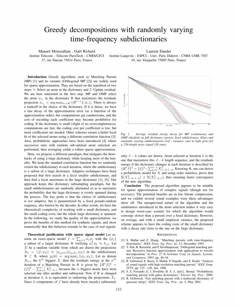
Greedy decompositions with randomly varyingtime-frequency subdictionaries

Manuel Moussallam , Gaël RichardInstitut Telecom - Telecom ParisTech - CNRS/LTCI

37, rue Dareau 75014 Paris, France

Laurent DaudetInstitut Langevin - ESPCI - Univ. Paris Diderot - CNRS UMR 7587

10, rue Vauquelin 75005 Paris, France

Introduction Greedy algorithms such as Matching Pursuit(MP) [1] and its variants (Orthogonal MP [2]) are widely usedfor sparse approximation. They are based on the repetition of twosteps: 1: Select an atom in the dictionary and 2: Update residual.We are here interested in the first step. MP and OMP selectthe atom φγi in the dictionary Φ that maximizes the residualsprojection φγi = arg maxφγ∈Φ |〈Rn−1f, φγ〉|. There is alwaysa tradeoff in the choice of the dictionary. If it is dense, we havea fast decay of the approximation error (as a function of theapproximation order), but computations get cumbersome, and thecost of encoding each coefficient may become prohibitive forcoding. If the dictionary is small (slight or no overcompleteness),computations are fast, the coding cost per coefficient is low, butmore coefficients are needed. Other schemes ensure a better localfit of the selected atoms using a different correlation function [3].Also, probabilistic approaches have been introduced [4] wheresuccessive runs with random sub-optimal atom selection areperformed, then averaging yields a robust sparse approximation.

Here, we propose a different paradigm, that mitigates the draw-backs of using a large dictionary while keeping most of the ben-efits. We keep the standard correlation function but we randomlyswitch the subdictionary at each iteration, where the subdictionaryis a subset of a large dictionary. Adaptive techniques have beenproposed that first search in a fixed smaller subdictionary, andthen find a local maximum in the large dictionary [1], [5]. Ourapproach keeps this dictionary subsampling paradigm, but thesmall subdictionaries are randomly alternated so as to maximizethe probability that the large dictionary is evenly spanned duringthe process. The key point is that the choice of subdictionaryis not adaptive, but is parametrized by a fixed pseudo-randomsequence, also known by the decoder. In other words, we have the(theoretical) complexity of working with a small dictionary, andthe small coding costs, but the whole large dictionary is spanned.In the following, we study the quality of the approximation: weprove the benefits of this method for synthetic signals, and shownumerically that this behavior extends to the case of real signals.

Theoretical justification with sparse signal model Let as-sume an exact-sparse model f =

Pj∈J αjφj with the φj

a subset of a larger dictionary Φ verifying φTj φk ≈ δj,k. LetX be a random variable from which are drawn the projectionsXk = |〈f, ψk〉| ≈ |αj0(k)〈φj0(k), ψk〉| in the subdictionaryΨ ⊂ Φ, where j0(k) = arg maxj |〈φj , ψk〉|. Let us denoteXk:J the kth biggest X , then the residuals energy at the nth

iteration of a Matching Pursuit in Ψ is given by ‖Rnf‖2 =‖f‖2 −

Pn−1k=0 X

2J−k:J because the n biggest atoms have been

selected one after another and subtracted. Now if Ψ is changedat iteration k, it is equivalent to redrawing the projections Xj .Since k components of f have already been (nearly) subtracted,

Fig. 1. Average residual energy decay for MP (continuous) andOMP (dashed) on full dictionary (green), fixed subdictionary (blue) andrandomly varying subdictionaries (red - variance zone in light grey) fora 256-length noisy signal (20 runs)

only J − k values are drawn. Atom selected at iteration k is theone that maximizes this J −k length sequence, and the residualsenergy if the dictionary changes at each iteration is described by‖Rnf‖2 = ‖f‖2−

Pn−1k=0 X

2J−k:J−k. Knowing Φ, one can derive

a probabilistic model for X and using order statistics, prove thatE(X2

J−k:J−k) ≥ E(X2J−k:J), thus ensuring faster convergence

of the new algorithm.Conclusion The proposed algorithm appears to be suitable

for sparse approximation of complex signals (though not forrecovery). The potential benefits are in low bitrate compression,and we exhibit several sound examples were these advantagesshow off. The unsupervised nature of the algorithm and therandomness introduced in the atom selection makes it very easyto design worst-case scenarii for which the algorithm wouldconverge slower than a pursuit over a fixed dictionary. However,on average, and with a small empirical variance, the proposedscheme appears to have the coding costs of the small dictionarywith a decay rate close to the one on the large dictionary.

REFERENCES

[1] S. Mallat and Z. Zhang, “Matching pursuits with time-frequencydictionaries,” IEEE Trans. Sig. Proc, no. 12, December 1993.

[2] Y. Pati, R. Rezaiifar, and P. Krishnaprasad, “Orthogonal matching pur-suit: Recursive function approximation with applications to waveletdecomposition,” in Proc. 27 th Asilomar Conf. on Signals, Systems,and Computers, 1993, pp. 40–44.

[3] R. Gribonval, E. Bacry, S. Mallat, P. Depalle, and X. Rodet, “Analysisof sound signals with high resolution matching pursuit,” IEEE Symp.TFTS, pp. 125 –128, Jun. 1996.

[4] S. E. Ferrando, E. J. Doolittle, B. A. J., and L. Bernal, “Probabilisticmatching pursuit with gabor dictionaries,” Elsevier Sig. Proc., 2000.

[5] R. Gribonval, “Fast matching pursuit with a multiscale dictionary ofgaussian chirps,” IEEE Trans. Sig. Proc., no. 5, May 2001.

115

1

A Sparsity based Regularization Algorithm withAutomatic Parameter Estimation

Damiana LazzaroDepartment of Mathematics, University of Bologna, Italy

Abstract—Regularization methods for the solution of ill-posed inverse problems can be successfully applied if aright estimation of the regularization parameter is known.While there exists a significant amount of research in theliterature on the development of appropriate parameterselection methods for Tikhonov regularization [7], untilnow the L1 regularization case has been considered in onlya few very recent papers, [1], [3], [4], [5], [6] that focusonly on Total Variation regularization. Among them, theonly method that, to our knowledge, does not require anyassumption on the noise level, has been proposed in[1]using variational distribution approximations. It updatesthe regularization parameter in an iterative manner andseem to be very effective for TV restoration problems wheninformation about the perturbation level is not available.Nevertheless, in spite of the good performance of thismethod, its computational cost is still too high for real-time practical applications. In this work we consider theimage deblurring problem and we evaluate its solutionusing a sparsity based regularization approach solved bymeans of the iterative forward-backward splitting method.The main contribution of this research is the proposal of anovel adaptive automatic rule for the estimation of the reg-ularization parameter in L1-based restoration problems,without requiring any assumption about the perturbationprocess. This rule, developed in the context of the iterativeforward-backward splitting method [2], exploits the infor-mation yielded by this approach to dynamically update theparameter value following the evolution of the objectivefunctional. The iterative algorithm automatically stops,when the parameter has reached a seemly near optimalvalue. A large number of numerical experiments confirmthat the proposed rule yields restoration results competitivewith those of the best state-of-the-art algorithms.

REFERENCES

[1] S.D. Babacan, R. Molina, and A.K. Katsaggelos , ParameterEstimation in TV Image Restoration using Variational Distri-bution Approximation, IEEE Trans. Image Process. Vol. 17, No.3, pp. 326–339, 2008.

[2] P.L. Combettes and V.R. Wajs , Signal Recovery by Proxi-mal Forward-Backward Splitting, SIAM Journal on MultiscaleModelling and Simulation,Vol.4, No. 4, pp. 1168–1200, 2005.

[3] H.Liao, F. Li, and M.K. Ng, Selection of Regularization Pa-rameter in Total Variation Image Restoration, Journal OpticalSoc. Am. A, Vol. 26, No. 11, pp. 2311–2320, 2009.

[4] Y. Lin, B. Wohlberg, and H. Guo, UPRE Method for TotalVariation Parameter Selection, Signal Processing, Vol. 90, pp.2546-2551, 2010.

[5] J.P. Oliveira, J.M. Bioucas-Dias, and M.A.T. Figureido,Adaptive Total Variation Image Deblurring: A Majorization-Minimization Approach, Signal Processing, Vol. 89, pp. 1683–1693, 2009.

[6] Y.W. Wen and A.M. Yip, Adaptive Parameter Selection for TotalVariation Image Deconvolution, Numer. Math.Theor. Meth.Appl., Vol. 2 No. 4, pp. 427–438, 2009.

[7] C.R. Vogel, Computational Methods for Inverse Problems,SIAM Philadelphia, 2002.

116

An unsupervised iterative shrinkage/thresholding algorithm forsparse expansion in a union of dictionnaries.

Matthieu Kowalski and Thomas RodetUniv. Paris-Sud – Laboratoire des Signaux et Systemes

Email: kowalski,[email protected]

Abstract—We are interested in hybrid/morphological decomposition ofsignals which can be expressed as the sum of two sparse components ina well choosen frame and a residual – such as images (edges+textures)or audio signal (tonals + transcients). Thanks to a Bernoulli-Gaussianprior on the synthesis coefficients, we derive an unsupervised algorithmin the spirit of ISTA with iteratively adapted thresholding/shrinkage. Themodel can be directly extended to joint-sparsity structure.

I. MODEL

Let U = un ∈ CNN1n=1 and V = vm ∈ CNN2

m=1 two frames ofCN . Let Λ and ∆ two finit subsets of N. We are interrested in” signalsy ∈ CN which admit an hybrid [1]/Morphological [3] expansion:

y =Xλ∈Λ

αλuλ +Xδ∈∆

βδvδ + n , (1)

where n ∈ CN is some noise, and where αλ, βδ ∈ C are the synthesiscoefficients. The sets Λ and ∆ are called the significance maps: ifλ ∈ Λ, then αλ 6= 0, and if λ /∈ Λ, then αλ = 0.

We choose a Bernoulli-Complex Gaussian prior which naturallyinduces sparsity. Let us definine the indicator variables:

Xn =

1 if n ∈ Λ0 otherwise ,

Xm =

1 if m ∈ ∆0 otherwise ,

(2)

with p and p the membership probabilities: ∀n , p = p(Xn =1) , ∀m , p = p(Xm = 1) . The corresponding model can thenbe written:

y =

N1Xn=1

Xnαnun +

N2Xm=1

Xmβmvm + n . (3)

In the following, we restrain ourself to the significance map Λ, allthe results can be directly applied to the map ∆. with the Bernoulli-Gaussian prior:

p(αλ|Xλ) = (1−Xλ)δ0 +XλCN (0, σ2, 0)

where the complex-Gaussian density are univariate.We finally assume n ∼ CN (0, σ2

0I) .

II. ALGORITHM DERIVATION

A. GEM

For the sake of simplicity, we rewrite (1):

y = Uα + Vβ + n = Φθ + n , (4)

with Φ = [UV] and θ = (αT ,βT )T .Insipired by [2], one can use a Generalized Expectation-

Maximization (GEM) strategy in order to maximize the penalizedlikelihood. By introducing the hidden varriable z, we have

z = θ + µn1 y = Φz + n2 , (5)

with n1 ∼ CN (0, I) and n2 ∼ CN (0, σ20I − µ2ΦΦT ) (µ2 <

σ0‖ΦΦ∗‖ ).

a) E-setp: : zt = θt + µ2

σ20Φ∗(y −Φθt) .

b) M-step: : the maps are first estimated by marginalization andmaximization

Λt+1, ∆t+1 = arg maxΛ,∆

Elog(p(Λ,∆|y, z, T ))|y,θt,Λt,∆t, T ,

then the coefficients θ:

θt+1

= arg maxθ

Elog(p(θ|Λt+1, ∆t+1,y, z, T )|y,θt,Λt,∆t, T

B. Maps estimation

For the significance map Λ we obtain:

Xt+1λ =

8<:1 if |ztλ| >r

(µ2+σ2)µ2

σ2 lnh

1−pp

µ2+σ2

µ2

i0 if not .

Remark: with a joint-sparsity model on the map, we obtain asimilar rule on the norm of groups of coefficients.

C. Coefficients estimation

We can then estimate the coefficients. If Xt+1λ = 1

θt+1λ = arg max

θλ

‖ztλ − θλ‖2µ2

+‖θλ‖2

2σ2=

ztλ1 + µ2/σ2

, (6)

and θt+1λ = 0 if not.

III. RESULTS

We apply such a strategy to a xylophone signal with a union ofGabor dictionnaries. We find σ2

0 = 0.001 (output SNR ' 16 dB) forσ2

0 = 0.0009 (input SNR ' 12 dB).

Fig. 1. Estimated Gabor coefficients of the two significance maps.

REFERENCES

[1] L. Daudet and B. Torresani. Hybrid representations for audiophonic signalencoding. Signal Processing, 82(11):1595–1617, 2002. Special issue onImage and Video Coding Beyond Standards.

[2] M. Figueiredo and R. Nowak. An em algorithm for wavelet-based imagerestoration. IEEE Transactions on Image Processing, 12(8):906–916,2003.

[3] J.-L. Starck, M. Elad, and D. L. Donoho. Image decomposition via thecombination of sparse representation and a variational approach. IEEETransaction on Image Processing, 14(10):1570–1582, 2005.

117

An Infeasible-Point Subgradient Algorithm and aComputational Solver Comparison for `1-Minimization

Andreas M. Tillmann∗Institute for Mathematical OptimizationTechnische Universitat Braunschweig

38106 Braunschweig, GermanyEmail: [email protected]

Dirk A. LorenzInstitute for Analysis and Algebra

Technische Universitat Braunschweig38106 Braunschweig, Germany


Marc E. PfetschInstitute for Mathematical OptimizationTechnische Universitat Braunschweig

38106 Braunschweig, GermanyEmail: [email protected]

Abstract—The `1-minimization problem min ‖x‖1 : Ax = b , alsoknown as Basis Pursuit (BP), has become important in Compressed Sens-ing due to its ability to yield the sparsest solution of an underdeterminedlinear system Ax = b under certain conditions. In the past few years, a lotof new algorithms solving (BP) or some (possibly regularized) variant of ithave been developed. We contribute the ISAL1 to the available spectrumof solvers, which is a specialization to (BP) of a new infeasible-pointsubgradient algorithm (ISA) for solving convex constrained minimizationproblems. In this extension of the classical projected subgradient methodsfrom nonsmooth optimization, the projections onto the feasible set needonly be approximated, thus allowing for a potentially large reduction ofthe computational burden. In particular, in ISAL1, inexact projectiononto x |Ax = b by performing a fixed small number of conjugategradient steps suffices to obtain convergence. Moreover, we will presentresults of an extensive computational comparison of various state-of-the-art `1-solvers, also including ISAL1. Furthermore, we show how a newoptimality check can speed up solvers and at the same time attain thetrue optimum (up to numerical precision).

I. INTRODUCTION

We propose a new infeasible-point subgradient algorithm (ISA)for the constrained minimization of convex functions. In contrast totypical projected subgradient schemes [1], the projection onto thefeasible set is only approximated in the ISA. Hence, the iterates maybe infeasible throughout the whole procedure, and still convergencecan be achieved under certain conditions. This allows to tackle prob-lems where computing the exact projections is expensive, especiallyfor large-scale instances.

Here, we focus on one such problem: Finding the minimal-`1-normsolution to an underdetermined linear system, i.e., (BP). This problemhas become very important in the field of Compressed Sensing,because under certain conditions (e.g., the RIP), it allows for exactrecovery of the minimum-support solution (`0-minimizer) of Ax = b,which is generally NP-hard to find.

Facing the vast choice of avaible (BP) solvers developed over thepast years, one may wonder which one is “the best”? Of course, thereare multiple answers (if any), depending on context, desired accuracy,etc. Here, we aim at an exact solution of (BP), without concernabout special cases or related problems such as `0-minimization. Tothis end, we conduct extensive numerical experiments with variousprominent `1-minimization solvers and the new ISAL1. We alsopresent an easily implementable optimality check and demonstrate itsusefulness by further computational experiments with several solvers.

II. NEW ALGORITHMS

The existing arsenal of solvers for (BP) includes methods based onvarious ideas, e.g., augmented Lagrangeans, interior-point schemes,spectral projected gradients or several penalized models. We proposeto add the ISA modification of projected subgradient methods.

∗ Supported by a DFG research grant.

A. ISA and ISAL1

The ISA iteration consists mainly of the iterate update xk+1 =P

εkX (xk − αkh

k), with stepsize αk, subgradient hk and the inexactprojection operator P εk

X for the feasible set X with accuracy εk.We investigated the ISA for several stepsize choices and obtainedconvergence results depending on the behaviour of the series ofprojection accuracies (εk).

ISAL1 specializes the ISA for solving (BP). For this particularproblem, projection onto x|Ax = b amounts to solving a linearsystem. This can be done by applying the method of conjugate gra-dients (CG). For the inexact projections in ISAL1, we derive boundson the CG residual norm which (among other things) guarantee themethod’s convergence. In practice, convergence can still be obtainedwhen only computing a fixed small number of CG steps.

B. Heuristic Support Evaluation

Our implementation of ISAL1 exhibited a typical drawback ofsubgradient methods: slow local convergence. This issue was success-fully overcome by integrating a Heuristic Support Evaluation (HSE)scheme, which allows “jumping” to the exact optimal solution byroughly checking a well-known optimality criterion for (BP) (see,e.g., [2]) on the estimated true solution support.

III. COMPUTATIONAL COMPARISON OF `1-SOLVERS

We carefully constructed a test set consisting of a wide rangeof (BP) instances, each with an optimal solution guaranteed tobe unique (by employing the ERC or the Source Condition). Wecompare several well-known algorithms which can provably solvegeneral (BP) instances, namely: SPGL1 (www.cs.ubc.ca/labs/scl/spgl1), YALL1 (yall1.blogs.rice.edu), `1-MAGIC (www.acm.caltech.edu/l1magic), SolveBP of SparseLab (sparselab.stanford.edu) (em-ploys PDCO), L1-Homotopy (users.ece.gatech.edu/∼sasif/homotopy),and ISAL1. As a reference, we also solved (BP) as a linear program,using the dual simplex method of CPLEX. Most available implemen-tations seem to go for a balanced speed-accuracy trade-off by default,i.e., aiming at fast termination with a medium-accuracy result whichhence not necessarily qualifies as an “exact solution”. Integratingthe HSE however shows that without needing to change algorithmicparameters, one can achieve both a speed-up and highest accuracy atthe same time. The potential of the HSE is supported by numericalexperiments with several solvers.

REFERENCES

[1] N. Z. Shor, Minimization Methods for Non-Differentiable Functions.Springer, 1985.

[2] J.-J. Fuchs, “On sparse representations in arbitrary redundant bases,” IEEETransactions on Information Theory, vol. 50, pp. 1341–1344, 2004.

118

On the relation between perceptrons and non-negative matrix factorization

Hugo Van hamme Department ESAT, Katholieke Universiteit Leuven, Leuven, Belgium.


A classical result in the theory of artificial neural networks (ANNs) is Cybenko’s theorem [1] which states that a perceptron with at least one hidden layer, sigmoidal output non-linearity and a sufficiently high, but finite, number of nodes can approximate any continuous and bounded function on a bounded domain within a given accuracy. This theorem has made multi-layer perceptrons (MLPs) a popular instrument for classification problems.

Perceptrons are inspired by the information processing in neurons [2], which makes them a trivial choice for modeling cognitive pro-cesses. Again inspired by the architecture of mammal brains, one would expect a several layers to be required in perceptron models. Deep MLP networks are however very difficult to train with the back-propagation algorithm. Supervisory information is needed and the fact that it cannot be provided for all hidden layers forms the crux of the problem.

In this paper, the parallels and differences between non-negative matrix factorization (NMF) and a single layer perceptron are discussed. NMF is capable of working without supervision but is equally capable of exploiting supervision information, which makes it very well suited to overcome the training problems in multilayer architectures. However, NMF additionally shows behavior that is observed in the brain: it performs lateral inhibition in a single layer and has masking properties.

NMF finds two factors W ∈ RN×R and H ∈ RR×T, with positive or zero entries such that a data matrix V ∈ RN×T with positive or zero entries is approximated by W H. The Frobenius norm and the (gene-ralized) Kullback-Leibler divergence (KLD) are considered here as cost function to express the proximity of V and W H. The weights W are learned unsupervisedly by applying NMF to training data V, where different training tokens occupy different columns in V.

In this contribution the multiplicative update algorithms proposed in [3] are cast in the flow diagrams of Figure 1. When classifying a single test token, V and H become vectors v and h, while W is assumed to be known from the training phase. Finding the NMF solution for h is compared to node activation in an ANN. The left pane shows the single layer perceptron which maps v to the hidden nodes y through the weight matrix W. A sigmoidal output non-linearity h(y) with diagonal structure is then applied. In NMF with Frobenius norm (middle), h(y) is replaced by the shaded box. The right pane shows the flow diagram for the KLD metric, which differs only from the middle pane by swapping the input projection Wt and the element-wise division ⊘. Both NMF problems are shown to have lateral inhibition behavior, i.e. a hidden node will deactivate nodes with similar weights (or neighboring neurons in the brain). Physically, inhibition leads to categorical perception. Mathema-

tically, inhibition corresponds to the case where the minimal (Frobenius or KLD) cost is achieved on the constraint boundary.

Supervisory information can be introduced in NMF by augmenting V with G such that. Gij = 1 if the i-th class is present in token j (and zero otherwise)

HW

X

V

G

≈

On test tokens, H can be computed as before from V and subsequently the class information G can be estimated by forming X H. In other words, with supervision, X acts like an output layer of a perceptron. With the previous result, NMF can be interpreted as an easily learnable perceptron with an output mapping that shows lateral inhibition, which adds to the cognitive motivation to use it as a building block for deep ANN structures.

Finally, the cognitive motivation is strengthened by observing that NMF also shows masking behavior in the sense that the sparsity pattern of H is robust to perturbations in V and not all changes to the input data affect H and hence the classification. A first masking mechanism is through L1 regularization of the cost function. Secondly, a positive bias term V0 can be added: find the best H s.t. V ≈ W H + V0. The case where V0 = W H0 for some H0 could model a reminiscent (decaying) neuron activation. The effect is that the cone of possible V spanned by the model W H + V0 is moved away from the origin, which will typically activate more constraints at the optimal H and can even lead to solutions that are not affected by the data V at all (masking).

In summary, there are strong parallels between a single layer perceptron and NMF, the latter showing the additional cognitive properties of unsupervised learnability, lateral inhibition and masking.

REFERENCES [1] G. Cybenko, “Approximations by superpositions of sigmoidal

functions,” in Mathematics of Control, Signals, and Systems, vol. 2, no. 4, pp. 303–314, 1989.

[2] F. Rosenblatt, “The Perceptron: A Probabilistic Model for Information Storage and Organization in the Brain,” in Psychological Review, vol. 65, pp. 386–408, 1958.

[3] D. Lee, and H. Seung, “Algorithms for non-negative matrix factorization,” in Advances in Neural Information Processing Systems, vol. 13, pp. 556–562, 2001.

Fig. 1: A flow diagram representation of a single layer perceptron (left), NMF with Frobenius norm (middle) and NMF with KLD (right). ⊗ and ⊘

are element-wise multiplication and division respectively. “z-1” is a memory over one iteration of the update formulae of [3].

119

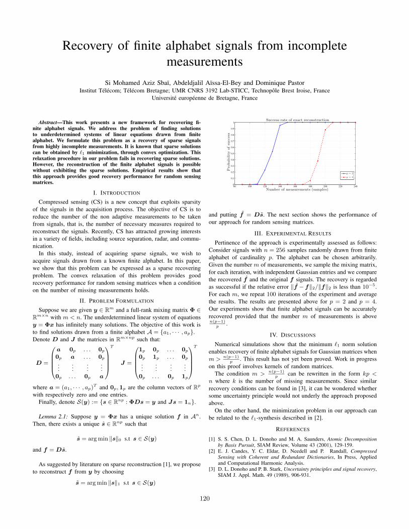
Recovery of finite alphabet signals from incompletemeasurements

Si Mohamed Aziz Sbaï, Abdeldjalil Aïssa-El-Bey and Dominique PastorInstitut Télécom; Télécom Bretagne; UMR CNRS 3192 Lab-STICC, Technopôle Brest Iroise, France

Université européenne de Bretagne, France

Abstract—This work presents a new framework for recovering fi-nite alphabet signals. We address the problem of finding solutionsto underdetermined systems of linear equations drawn from finitealphabet. We formulate this problem as a recovery of sparse signalsfrom highly incomplete measurements. It is known that sparse solutionscan be obtained by `1 minimization, through convex optimization. Thisrelaxation procedure in our problem fails in recovering sparse solutions.However, the reconstruction of the finite alphabet signals is possiblewithout exhibiting the sparse solutions. Empirical results show thatthis approach provides good recovery performance for random sensingmatrices.

I. INTRODUCTION

Compressed sensing (CS) is a new concept that exploits sparsityof the signals in the acquisition process. The objective of CS is toreduce the number of the non adaptive measurements to be takenfrom signals, that is, the number of necessary measures required toreconstruct the signals. Recently, CS has attracted growing interestsin a variety of fields, including source separation, radar, and commu-nication.

In this study, instead of acquiring sparse signals, we wish toacquire signals drawn from a known finite alphabet. In this paper,we show that this problem can be expressed as a sparse recoveringproblem. The convex relaxation of this problem provides goodrecovery performance for random sensing matrices when a conditionon the number of missing measurements holds.

II. PROBLEM FORMULATION

Suppose we are given y ∈ Rm and a full-rank mixing matrix Φ ∈Rm×n with m < n. The underdetermined linear system of equationsy = Φx has infinitely many solutions. The objective of this work isto find solutions drawn from a finite alphabet A = a1, · · · , ap.Denote D and J the matrices in Rm×np such that:

D =

a 0p . . . 0p

0p a . . . 0p

......

......

0p . . . 0p a

T

J =

1p 0p . . . 0p

0p 1p . . . 0p

......

......

0p . . . 0p 1p

T

where a = (a1, · · · , ap)T and 0p, 1p are the column vectors of Rp

with respectively zero and one entries.Finally, denote S(y) := s ∈ Rnp : ΦDs = y and Js = 1n.

Lemma 2.1: Suppose y = Φx has a unique solution f in An.Then, there exists a unique s ∈ Rnp such that

s = arg min ‖s‖0 s.t s ∈ S(y)

and f = Ds.

As suggested by literature on sparse reconstruction [1], we proposeto reconstruct f from y by choosing

s = arg min ‖s‖1 s.t s ∈ S(y)

80 100 120 140 160 180 200 220 2400

0.1

0.2

0.3

0.4

0.5

0.6

0.7

0.8

0.9

1

Number of measurements (samples)

Probabilityofsu

ccess

Success rate of exact reconstruction

p = 2

p = 4

and putting f = Ds. The next section shows the performance ofour approach for random sensing matrices.


Pertinence of the approach is experimentally assessed as follows:Consider signals with n = 256 samples randomly drawn from finitealphabet of cardinality p. The alphabet can be chosen arbitrarily.Given the number m of measurements, we sample the mixing matrix,for each iteration, with independent Gaussian entries and we comparethe recovered f and the original f signals. The recovery is regardedas successful if the relative error ‖f − f‖2/‖f‖2 is less than 10−5.For each m, we repeat 100 iterations of the experiment and averagethe results. The results are presented above for p = 2 and p = 4.Our experiments show that finite alphabet signals can be accuratelyrecovered provided that the number m of measurements is aboven(p−1)

p.

IV. DISCUSSIONS

Numerical simulations show that the minimum `1 norm solutionenables recovery of finite alphabet signals for Gaussian matrices whenm > n(p−1)

p. This result has not yet been proved. Work in progress

on this proof involves kernels of random matrices.The condition m > n(p−1)

pcan be rewritten in the form kp <

n where k is the number of missing measurements. Since similarrecovery conditions can be found in [3], it can be wondered whethersome uncertainty principle would not underly the approach proposedabove.

On the other hand, the minimization problem in our approach canbe related to the `1-synthesis described in [2].

REFERENCES

[1] S. S. Chen, D. L. Donoho and M. A. Saunders, Atomic Decompositionby Basis Pursuit, SIAM Review, Volume 43 (2001), 129-159.

[2] E. J. Candes, Y. C. Eldar, D. Needell and P. Randall, CompressedSensing with Coherent and Redundant Dictionaries, In Press, Appliedand Computational Harmonic Analysis.

[3] D. L. Donoho and P. B. Stark, Uncertainty principles and signal recovery,SIAM J. Appl. Math. 49 (1989), 906-931.

120

Adding Dynamic Smoothing to Mixture Mosaicing SynthesisGraham Coleman

Music Technology GroupUniversitat Pompeu Fabra

Barcelona, SpainEmail:[email protected]

Jordi BonadaMusic Technology GroupUniversitat Pompeu Fabra

Barcelona, SpainEmail: [email protected]

Esteban MaestreCenter for Computer Research in Music and Acoustics

Stanford UniversityStanford, USA


Abstract—Recent works in sound mosaicing synthesis [1], [2] haveproposed algorithms that permit instantaneous mixtures of severalsources atoms, based on sparse signal representation techniques. Wepropose combining l1 regularization with linear dynamical smoothingas in the Kalman filter (also in [3], [4]) to promote desired transitionsbetween atoms, while adapting the generic approach to the mixturemosaicing context. Furthermore, we modify the dynamics cost slightlyto further promote sparse scores in the case of non-negativity. This is awork in progress in which we can present some sound examples, but forwhich the proposal is not fully validated.

I. INTRODUCTION

Mosaicing, a form of sample-based sound synthesis, consists intransforming and compositing disparate source sound segments froma database so that the result will match perceptual features (descrip-tors) of a target sequence. Classical methods [5], [6] consideredmatching a single source segment to a given target context (frame),while more recent methods [1], [2] consider sparse mixtures ofmultiple source segments at once.

Several criteria for these systems concern the dynamics–thechanges from frame to frame–of the composition, or more abstractly,the sampling process that generates it. Do the descriptors of thesource units change too much from frame to frame (continuity)?Do the transformation parameters applied to the sources changerapidly from frame to frame (transformation continuity)? Does thesampling process maintain a steady context within the source materialby choosing contiguous blocks of material from the original sourcecontext, or does it jump around (contiguity)? By modeling dynamicswe can search or sample sequences or mixtures that have desiredproperties above.

II. PROPOSAL

Given a matrix or linear operator D describing favored atomtransitions from state to state, one way of generalizing it to mixturesof atoms is simply considering a form of linear dynamics where:xt+1 = Dxt + wt. xt and xt+1 are mixture vectors for time stepst and t + 1, wt represents innovation, or deviance from expecteddynamics.

Combining the smoothing version of the Kalman filter with an l1regularization term as in Basis Pursuit Denoising (BPDN) would giveus the following program:

minx

T∑t=1

‖Axt − bt‖22 + λ1

T∑t=2

‖Dxt−1 − xt‖+ λ2

T∑t=1

‖xt‖1 (1)

Under the scheme given by Problem 2, if the transition matrix Dgives a number of possibilities for a given atom, the most likely suc-cessor state (where the innovation cost is zero) will include nonzeroweights on all of those possibilities. Therefore, when D includesmany alternatives for transitions between atoms, the innovation costand the sparsity cost are working against each other.

In our application, where weights are constrained to be non-negative, we propose modeling alternatives using an innovation costwhere only positive innovation is penalized, that is having no costwhen weights decrease (state is closer to sparsity than deterministicdynamics). We implement this by introducing a non-negative dummyvariable y:

minx

T∑t=1

‖Axt − bt‖22 + λ1

T∑t=2

‖Dxt−1 − xt − yt‖+ λ2

T∑t=1

‖xt‖1

(2)where both x and y are constrained to be elementwise non-negative.In this scheme, successor states are not penalized for atom transitionalternatives not taken, only for unlikely transitions that are taken.

III. OTHER APPROACHES

Several other approaches are also likely feasible for encouragingdynamics in synthesis. For one, we could extend the Kalman filterobjective with a nonlinear model, which may render the objectivefunction non-convex. In this case, heuristic methods based on convexrelaxation such as DC Algorithms (DCA) could be used to findheuristic solutions quickly.

Sampling or Monte-Carlo approaches are also feasible. In partic-ular, particle filters (Sequential Monte Carlo) have been used fortracking, and allow both nonlinear dynamics, and use non-parametricestimates for the states.

Finally, so called greedy signal decomposition methods couldperhaps be adapted to account for dynamics. In practice this wouldbe analogous to sampling in many ways. Perhaps a good example ofthis in image synthesis would be Ashikhmin [7].

REFERENCES

[1] M. D. Hoffman, P. R. Cook, and D. M. Blei, “Bayesian spectral matching:Turning young MC into MC hammer via MCMC sampling.”

[2] G. Coleman, E. Maestre, and J. Bonada, “Augmenting sound mosaicingwith Descriptor-Driven transformation,” in Proceedings of DAFx 2010,Graz, Austria.

[3] A. Charles, M. S. Asif, J. Romberg, and C. Rozell, “Sparsity penalties indynamical system estimation.”

[4] M. S. Asif, A. Charles, J. Romberg, and C. Rozell, “Estimation anddynamic updating of time-varying signals with sparse variations,” 2011.

[5] A. Zils and F. Pachet, “Musical mosaicing,” Digital Audio Effects (DAFx),2001, here are where the notes go for annotated bibliographies.

[6] D. Schwarz, “Data-Driven concatenative sound synthesis,” Ph.D. disserta-tion, 2004. [Online]. Available: http://recherche.ircam.fr/equipes/analyse-synthese/schwarz/thesis/

[7] M. Ashikhmin, “Synthesizing natural textures,” in Proceedings of the2001 symposium on Interactive 3D graphics, ser. I3D ’01, 2001, p.217–226, ACM ID: 364405.

121

Block-Sparse Recovery via Convex OptimizationEhsan Elhamifar

Johns Hopkins UniversityRene Vidal


Abstract—We consider the problem of recovering block-sparse signals,i.e. signals that can be written as linear combination of vectors drawnfrom of a union of a few subspaces. To find a block-sparse representationof a signal, we consider two classes of non-convex programs based onminimizing a mixed `q/`0 quasi-norm (q ≥ 1) and their convex `q/`1

relaxations. The first class directly penalizes the norm of the coefficientblocks, while the second one penalizes the norm of the reconstructedvectors from the blocks of the dictionary. For each class of convexprograms, we provide conditions under which they are equivalent to theoriginal non-convex programs. We apply our methods to classificationtasks and obtain significant improvements relative to the state-of-the-art.

I. INTRODUCTION

The recovery of block-sparse signals involves solving a system oflinear equations of the form

y = Bc =[B[1] · · · B[n]

]c, (1)

where B consists of n blocks B[i] ∈ RD×mi whose atoms are gen-erated by a di ≤ mi dimensional subspace Si. The main differencewith respect to classical sparse recovery is that the nonzero elementsfor the solution of (1) correspond to a few blocks rather than a fewelements of B. We say that a vector c> =

[c[1]> · · · c[n]>

]is

k-block-sparse, if at most k blocks c[i] ∈ Rmi are nonzero.The problem of finding a representation of a signal y that uses the

minimum number of blocks of B can be cast as

P`q/`0 : min

n∑i=1

I(‖c[i]‖q > 0) subj. y = Bc, (2)

where I(·) is the indicator function and q ≥ 0. Since (2) is an NP-hard problem, we consider the following `1 relaxation of P`q/`0

P`q/`1 : min

n∑i=1

‖c[i]‖q subj. y = Bc, (3)

which is a convex program for q ≥ 1. We also propose an alternativeapproach based on solving the non-convex program for q ≥ 0

P ′`q/`0: min

n∑i=1

I(‖B[i]c[i]‖q > 0) subj. y = Bc. (4)

While P`q/`0 penalizes the norm of the coefficient blocks, P ′`q/`0

penalizes the norm of the reconstructed vectors from the blocks. SinceP ′`q/`0

is NP-hard, for q ≥ 1, we consider the `1 convex relaxation

P ′`q/`1 : min

n∑i=1

‖B[i]c[i]‖q subj. y = Bc. (5)

In what follows, we derive conditions under which the convexprograms P`q/`1 and P ′`q/`1

, respectively, are equivalent to P`q/`0

and P ′`q/`0for arbitrary q ≥ 1. In doing so, we allow for an arbitrary

number of atoms in each block of the dictionary, thus relaxing theassumption of uniqueness of the representation made by state-of-the-art methods, which restrict the blocks of a dictionary to havelinearly independent atoms. To characterize the relation betweenblocks of a dictionary, we introduce the notion of mutual/cumulativesubspace coherence, which can be thought of as natural extensionsof mutual/cumulative coherence from one to multiple subspaces.

Definition 1: Mutual subspace coherence is defined as

µS , maxi 6=j

µ(Si,Sj), (6)

where µ(Si,Sj) is the cosine of the smallest principal angle betweensubspaces Si and Sj . k-cumulative subspace coherence is defined as

ζk , maxΛk

maxi/∈Λk

∑j∈Λk

µ(Si,Sj), (7)

where Λk is a subset of k different elements from 1, . . . , n.To characterize the relation among atoms of a dictionary, we define

the following notions.Definition 2: For a dictionary B, we define εq as the smallest

constant such that for all i there exists a full column-rank submatrixB[i] ∈ RD×di of B[i] such that for all c[i], we have

(1− εq)‖c[i]‖2q ≤ ‖B[i]c[i]‖22 ≤ (1 + εq)‖c[i]‖2q. (8)

Define σq as the smallest constant such that for all i and c[i]

‖B[i]c[i]‖22 ≤ σq‖c[i]‖2q. (9)

Roughly speaking, εq characterizes the best q-restricted isometryproperty among all submatrices of B[i] that span subspace Si. Also,from definition, we have 1 + εq ≤ σq . We have the following result.

Theorem 1: For a signal that has a k-block-sparse representationin B, the solution of P`q/`1 is equivalent to that of P`q/`0 , if√

σq/(1 + εq) ζk + ζk−1 < (1− εq)/(1 + εq). (10)

A stronger sufficient condition is given by

(k√σq/(1 + εq) + k − 1)µS < (1− εq)/(1 + εq). (11)

Similar conditions can be found for the equivalence between P ′`q/`1

and P ′`q/`0for arbitrary q ≥ 1 and for dictionaries with arbitrary

number of atoms in each block. We refer the reader to [1] for details.

II. APPLICATION TO FACE CLASSIFICATION

Assume we have a training set from P classes, where each classconsists of the data drawn from a few subspaces. That is,

B = [ B[1] B[2] B[3]︸︷︷︸Class1

| · · · |B[n− 1] B[n]︸︷︷︸ClassP

] (12)

Given a test data y that belongs to one of the classes, the goalis to find the class to which the test example belongs. Since eachclass consists of a few blocks of the dictionary, the class of the testexample can obtained by finding the minimum number of blocks thatreconstruct y. Thus, the classification problem can be cast as a block-sparse recovery problem. We applied the proposed convex optimiza-tion programs for face classification on the Extended YaleB Database,which consists of a total of 2432 face images for 38 individualscorresponding to P = 38 classes. Our results improve the state-of-the-art classification results by 10% on the dataset.

REFERENCES

[1] E. Elhamifar and R. Vidal, “Robust classification via structured sparserepresentation,” in CVPR, 2011.

122

Performance Limits of the Measurements on CompressiveSensing for Multiple Sensor System

Sangjun Park, Hwanchol Jang and Heung-No Lee*Gwangju Institute of Science and Technology, South Korea. Email: sjpark1,hcjang,heungno*@gist.ac.kr

Abstract—A performance analysis of Multiple-Sensor-System(MSS) ona compressive sensing(CS)[1] w.r.t. the per-sensor-measurements(PSM) isstudied. In the proposed MSS, sensors make measurements using CSand the decoder jointly recover signals from them. We obtain the upperbound on the recovery failure probability for given K-sparse signals,derive the relationship between PSM and the number of sensors(S) forthe recovery. We examine the effect of SNR and S for the recovery. Weuse the concept of joint typicality proposed by Shannon[6]. We showsthat PSM converges to the sparsity(K) as S increases for given K-sparsesignals. Theoretical result is consistent with [3][4][5].

Index Terms—Compressive Sensing, Multiple Sensor System. JointRecovery.

I. INTRODUCTION AND MOTIVATION

Multiple-Sensor-System (MSS) deploys many sensors to a limitedregion and uses them to measure the signal from a common infor-mation source in different locations. In MSS, high resolution signalcan be obtained as many sensors are used to measure a commonphenomenon from many places. However, the coverage areas of sen-sors may significantly overlap with each other as they are distributedin a limited region. This causes redundancy in the measurementsignal. The transmission of the redundant signal to the fusion centeris a significant communication costs. There is tradeoff between theresolution and the redundancy on the number of sensors. To work onthis tradeoff relationship, we use the idea of the compressive sensing[1]. CS reduces the number of measurements while it recovers thesignal perfectly. Using this technique, it is possible to reduce theredundancy and obtain high resolution simultaneously by reducingthe per-sensor-measurements (PSM).

To investigate our problem, we propose to use an informationtheoretic tool, the concept of Jointly Typicality [6]. It was also usedby Akcakaya and Tarokh [2] for the single sensor case. Using thistool, we can derive the upper bound on the failure probability as afunction of PSM, the number of sensors, the sparsity and the noisevariance.

Clearly, the MSS problem is different from a single sensor systemin many aspects. For an appropriate modification of the tool for MSSproblem, we should consider these differences. One big difference isthe signal correlation among the sensors. For a successful extension,we use the inter-signal correlation in the system model and thedecoder also takes advantage of this signal correlation for a signalrecovery. To make the correlation model, we assume that each sensorhas the same sparsity and shares the same support set which is theset of indices for the non-zero elements. Obviously, in the recovery,the decoder using this prior information gains benefits.

II. THEOREMS

Theorem 1: Let the rank of Fs,J be K for each s and J be anycandidate set, M > K, σ2 = min(

∑i∈I\J xs(i)

2) over s, andδ > 0. Then, PFail|x converges to zero as the number of sensorsincreases.

Theorem 2: Let the rank of Fs,J be K for each s and J be anycandidate set, M > K, σ2 = min(

∑i∈I\J xs(i)

2) over s, δ > 0,

Si be the number of sensors of the ith MSS, σ2i be the noise variance

of the ith MSS and P1Fail|x ≤ γ. If the noise variance increases,i.e.,σ2

1 < σ22 , then, the sufficient condition for P2Fail|x ≤ γ is

S2 ≥ S1 max

f(δσ21

MM−K

)f(δσ22

MM−K

) , g(

σ21

σ2min,1

+ δσ2min,1

MM−K

)g

(σ22

σ2min,2

+ δσ2min,2

MM−K

) .

(1)We note that f(x) = log(1 + x) − x, g(x) = log(x) − x + 1,

σ2min,i ≡ min(

∑j∈I\J xs(j)

2) + σ2i over s and J , J denotes any

subset with size K expect for I and I denotes the set whose entriesare corresponding to indices of the nonzero elements in signal. Alltheorems will be explained in the next section.

III. CONTRIBUTIONS AND CONCLUSIONS

We use the described correlation model with noisy observation.First, we have found how many per-sensor-measurements (PSM) areneeded for successful recovery in the MSS problem. As the numberof sensors increases, how does PSM change? There is a limit we havefound. We will show this behavior and will show how PSM dependson the sparsity. We have Theorem 1 that the infimum of PSM is thesparsity obtained as the number of sensors increases. Different fromthe results in [3], [4], [5], the work of ours gives analytical results.Our analysis works for a small number of sensors as well. Second, wehave shown that the decoder which uses the prior information obtainsbenefit in terms of the Signal to Noise Ratio (SNR). Specifically,Theorem 2 tells us how the required SNR decreases as the numberof sensors changes.

IV. ACKNOWLEDGMENT

This work was supported by the National Research Foundation ofKorea (NRF) grant funded by the Korea government (MEST) (Do-Yak Research Program, N0. 2010-0017944).

REFERENCES

[1] Dvaid L. Donoho, “Compressive sensing,” IEEE Trans. On InformationTheory, vol. 52, pp. 1289-1306, 2006.

[2] Mehmet Akcakaya and Vahid Tarokh, ”Shannon-Theoretic Limits onNoisy Compressive Sampling”, IEEE Trans. On Information Theory,vol. 56, 2010.

[3] S. Sarvotham et. al, ”Analysis of the DCS one-stage greedy algorithm forcommon sparse supports, Technical Report TREE-0503: Rice University,Department of Electrical and Computer Engineering,” Oct. 2005.

[4] D.Baron et. al ”Distributed compressive sensing,” 2009.[5] Pablo Vinuelas-Peris and Antonio Artes-Rodriguez, ”Bayesian Joint

Recovery of Correlated Signals in Distributed Compressed Sensing,”2010 2nd International Workshop on Cognitive Information Processing

[6] Thomas M. Cover and Joy A. Thomas, ”Elements of Information Theorysecond Edition,” 2006

123

Message Passing Aided Least Square Recovery forCompressive Sensing

Jaewook Kang, Heung-No Lee and Kiseon KimGwangju Institute of Science and Technology, South Korea. Email: jwkkang,heungno,[email protected]

I. INTRODUCTION AND MOTIVATION

Compressive sensing (CS) have got attention as a promising signalprocessing technique to reduce information rate of sparse signals[1]. One line of CS related researches are to devise low complexityrecovery algorithms since the conventional L1-norm based recoveryalgorithms still have high computational complexity for practicalapplications. Recently, a few researchers have made an attempt toapply probabilistic message passing (PMP) ideas to CS recovery [2],[3] since PMP has provided a successful solution for low complexitydecoding while showing suboptimal performance in channel codingproblems, such as low-density parity check codes [4].

Motivated by such previous works, in this paper, we propose anew least square estimation (LSE) based CS recovery algorithm byapplying PMP, called PMP-LSE. It is well known that CS recoveryis basically an underdetermined system and it can be reformed asan overdetermined system with the support set information (SI).Therefore, in the proposed algorithm, PMP undertakes to find theSI of the signal to reform the recovery to an overdetermined case,and then LSE completes the recovery using the SI. Mainly, PMP-LSE has two strong benefits. First, PMP-LSE shows outstandingperformance with noisy measurements by removing the noise effectfrom elements belonging to the non-support set. Second, PMP-LSEprevents the recovery from diverging. Under certain conditions, PMPbased algorithms fails in the recovery due to divergence caused by alarge number of iterations. In the algorithm, however, the possibilityof the divergence highly decreases since PMP is only used to searchthe SI with a few iterations.

II. PROBLEM SETUP

We consider a sparse signal x ∈ RN whose sparsity is character-ized by q, named sparsity rate. With the sparsity rate q, each elementof x belongs to the support set denoted by S. Hence, |S| correspondsto Binomial random variable with B(N, q). Let xS ∈ R|S| denotea vector consisting of nonzero elements belonging to S, and assumethat each element of xS follows Gaussian distribution with N(0, σ2

x).We also assume that the sensing matrix is a well-designed binarymatrix, i.e., Φ ∈ 0, 1M×N , according to [5] such that themeasurements y ∈ RM are generated by y = Φx. Then, noisymeasurements z ∈ RM at the decoder are described as z = y + n,where each element of n ∈ RM is Gaussian noise with N(0, σ2

n).

III. ALGORITHM

The algorithm is divided into two parts: PMP and LSE.i) PMP: PMP consists of two kinds of probability calculations basedon Bayesian rule: Variable to check message (VCM, vi→j) and checkto variable message (CVM, cj→i) calculation where i and j indicatethe index of elements of x and z, respectively.

VCM : vli→j := pxi|z = Clpxi ×

∏k:ϕki=1,k =j

cl−1k→i (1)

12 14 16 18 20 22 24 26 28 300

0.5

1

1.5

SNR <dB>

MM

SE

CS-BP

PMP-LSE, Vth=sigma/8

PMP-LSE, Vth=sigma/4

Fig. 1. MMSE performance of PMP-LSE (N=100,M=80,q=0.1,Niter=3)

CVM : clj→i := Pzj |xi = Pzj −

∑k:ϕjk=1,k =i

xk + xi|xi

= pzj |any xk : ϕjk = 1 ∗ vlk1→j ∗ · · · ∗ vl

kLj−1→j(2)

Here, l is the number of iteration, ϕji is the (j, i) th element of Φ, Lj

is the number of ones in jth row of Φ, and Cl is the normalizationconstant for lth VCM. And, ∗ indicates the convolution operation.At each iteration, PMP updates VCM and CVM by exchanging theprobabilistic messages among the elements of x and z. After a fewiterations, PMP distinguish the elements of the support set with acertain threshold denoted by Vth.ii) LSE: Once the SI is given, xS is easily estimated only usingthe corresponding columns of Φ, denoted by ΦS, i.e., xS =(ΦT

SΦS)−1ΦTSz. By combining the SI and xS, PMP-LSE completes

to find the recovered signal x.

IV. NUMERICAL RESULTS

To demonstrate the performance, we simulated PMP-LSE with CS-BP [2]. Figure 1 plots the MMSE per elements as a function of SNRfor variety of thresholds with three PMP iterations. Figure 1 showsthat PMP-LSE outperforms CS-BP notably in low SNR region. Thereason is that PMP-LSE prevents the corruption of zero elementsfrom the noise effect by pre-detecting the support set using PMP.

ACKNOWLEDGMENT

This work was supported by the National Research Foundation ofKorea (NRF) grant funded by the Korea government(MEST) (HaekSim Research Program, N0. 2010-0026407)

REFERENCES

[1] D.L. Donoho, “Compressive sensing,” IEEE Trans. On InformationTheory, vol. 52, pp. 1289-1306, 2006.

[2] D. Baron, S. Sarvotham, and R. Baraniuk, ”Bayesian CompressiveSensing via Belief Propagation,” IEEE Trans. Signal Process., Vol. 58,No. 1, pp. 269-280, Jan. 2010.

[3] D.L. Donoho, A. Maleki and A. Montanari, ”Message passing algorithmsfor compressed sensing: I. Motivation and construction,” Proc. IEEEITW, Cairo, Egypt, Jan. 2010.

[4] R.G.Gallager, Low-Density Parity Check Codes, MIT Press: Cambridge,MA, 1963.

[5] T. Richardson, A. Shokrollahi, and R. Urbanke, ”Design of capacityapproaching irregular low-density parity check codes,” IEEE Trans.Inform. Theory, vol. 47, pp. 619-637, Feb. 2001.

124

Matrix-free Interior Point Method for Compressed SensingProblems

Kimonas FountoulakisSchool of Mathematics and Maxwell Institute

The University of EdinburghMayfield Road, Edinburgh EH9 3JZ

United Kingdom.Email: [email protected]

Jacek GondzioSchool of Mathematics and Maxwell Institute

The University of EdinburghMayfield Road, Edinburgh EH9 3JZ

United Kingdom.Email: [email protected]

Abstract—We consider a class of optimization problems for sparsesignal reconstruction which arise in the field of Compressed Sensing(CS). A plethora of approaches and solvers exist for such problems, forexample GPRS, SparseLab, `1 `s, `1 magic, FPC AS to mention a few.

Compressed Sensing applications lead to very well conditioned opti-mization problems and therefore can be solved easily by simple first-ordermethods. In this work we demonstrate that a second-order method suchas an interior point algorithm can be specialized for the CS problemsand offer a competitive alternative to the existing approaches. The newapproach is based on the Matrix-free Interior Point Method [1] in whichan iterative (Krylov-subspace) method is employed to compute an inexactNewton direction. The matrix-free IPM does not require an explicitstorage of the constraint matrix but accesses it only to get the matrix-vector products. It is therefore well-suited for solving large scale problemsbecause it can take full advantage of the low-complexity fast matrix-vectoroperations. A partial Cholesky preconditioner is employed to acceleratethe convergence of the Krylov-subspace method. The computation ofthe preconditioner requires only matrix-vector products and fits intothe matrix-free regime. Computational experience on the medium scaleone-dimensional signals (n = 4096) confirms that the new approach isefficient and compares favourably with other state-of-the-art solvers.

I. INTRODUCTION

Interior point methods (IPMs) for linear and convex quadratic pro-gramming enjoy an unequalled worst-case complexity result. Indeed,they deliver a ε-accurate solution to such problems inO(

√n ln(1/ε))

iterations, where n is the problem dimension. IPMs are usuallyapplied to solve problems to a high degree of accuracy (small ε, say,10−8). However, it is straightforward to specialize them to work in asignificantly less demanding environment such as that of CompressedSensing where accuracy of ε = 10−1 is often all the user wishes for.

The optimization problems arising in Compressed Sensing applica-tions are very well-conditioned and therefore trivial from optimizationpoint of view. This explains why the simple approaches based onprojected gradient can solve these problems so efficiently. In thisshort note we argue that a specialized Interior Point Method (IPM),implemented in the HOPDM solver, can offer a competitive approachfor optimization problems arsing in Compressed Sensing applications.

II. FUNDAMENTALS OF MATRIX-FREE IPM

The interior point solver for convex quadratic programming needsto solve a particular weighted least-squares problem at each iteration.This is usually done by a direct approach which is based on theCholesky factorization. In a relaxed environment in which only anapproximate solution of the problem is requested it is advantageousto employ an iterative method such as for example the conjugategradient algorithm to solve the underlying system of linear equations.An exact Newton method employed in the standard IPM is thenreplaced with an inexact one [1].

TABLE I: Comparison table

SolverR. Gaussian. Orth. R. Gaussian. Part. Hadamard

CPU times (sec)CPU MSE CPU MSE CPU MSE

HOPDM 8.50 7.5e-3 12.36 1.5e-2 8.61 1.1e-2GPSR 6 1.61 4.0e-4 1.15 1.9e-4 1.08 1.7e-4FPC AS 0.53 7.3e-4 0.75 1.3e-4 0.75 1.1e-4PDCO 10.29 1.8e-2 11.72 8.2e-2 10.04 7.6e-3`1 `s 8.60 4.0e-4 5.50 1.9e-4 4.47 1.7e-4

To achieve fast convergence of the iterative algorithm one needs touse a suitable preconditioner for the linear system. The preconditionerin the Matrix-Free IPM [2] is constructed in two steps. Firstly, thelinear algebra subproblem is regularized and secondly a low-rankpartial Cholesky factorization for this regularized system is computed.The process of computing the preconditioner does not require explicitaccess to the Jacobian matrix: only matrix-vector multiplications withthis operator are needed and therefore the approach can take fulladvantage of the low-complexity matrix-vector operations which relyon the low-parametric representation of the Jacobian matrices.

III. COMPUTATIONAL EXPERIENCE

We consider CS problems analogous to the ones in [3]. The recon-struction of the sparse signals is achieved via random Gaussian (R.Gaussian.), orthonormalized random Gaussian (Orth. R. Gaussian.)and partial Hadamard (Part. Hadamard.) m× n sensing matrices.

The table (I) shows the computational time and the mean squarederror (MSE = ‖x−x‖2

n) of the reconstructed signals for the matrix-

free HOPDM and some of the existing state-of-the-art solvers:GPRS, FPC AS, SparseLab (PDCO), `1 `s.

In the case of table (I), sparse signals n = 4096 with 160 ran-domly placed spikes were generated. The sensing matrices: Gaussian,orthonormalized Gaussian and partial Hadamard with m = 1024 andn = 4096 were used. Moreover, white noise with σ2 = 10−4 isadded in the sampled signal and finally, the optimality tolerance forthe termination criteria of each solver has been set to 10−2.

REFERENCES

[1] R. S. Dembo and S. C. Eisenstat and T. Steihaug, Inexact NewtonMethods, SIAM Journal on Numerical Analysis 19 (1982) 400–408.

[2] J. Gondzio, Matrix-Free Interior Point Method, Computational Opti-mization and Applications, Published online: October 15, 2010. DOI:10.1007/s10589-010-9361-3

[3] S. Kim, K. Koh, M. Lustig, S. Boyd, and D. Gorinvesky, Amethod for large-scale `1-regularized least squares problems withapplications in signal processing and statistics, Tech. Report, Dept.of Electrical Engineering, Stanford University, 2007. Available atwww.stanford.edu/˜boyd/l1 ls.html

125

A Block-Based Approach to Adaptively Biasthe Weights of Adaptive Filters

Luis A. Azpicueta-RuizDept. of Signal Theory and Communications

Universidad Carlos III de Madrid, 28911 Leganés, Madrid, Spain.Email: [email protected]

Jerónimo Arenas-GarcíaDept. of Signal Theory and Communications

Universidad Carlos III de Madrid, 28911 Leganés, Madrid, Spain.Email: [email protected]

I. EXTENDED ABSTRACT

Adaptive filters are crucial in many signal processing applications.Recently, a simple configuration was presented to introduce a biasin the estimation of adaptive filters using an adaptively adjustedmultiplicative factorα(n), showing important gains in terms of meansquare error with respect to standard adaptive filter operation, mainlyfor low signal to noise ratios (see [1]).

In this paper, we modify that scheme to obtain further ad-vantages by splitting the adaptive filter coefficients intoM non-overlapping blocks, and employing a different scaling factorαm withm = 1, ..., M for the coefficients in each block. In this way, biasvs variance compromise is managed independently in each block,allowing an enhancement if the energy of the unknown system isnon-uniformly distributed, as it is the case of sparse identification.

The proposed scheme is based on a blockwise decomposition ofan adaptive filterw(n) with length N in blocks of P = N/Mcoefficients each. In order to implement a scheme able to selectivelybias certain blocks of coefficients, we can multiply the correspondingcoefficients by a shrinkage factorαm to be adjusted according tomean squared error (MSE) performance. The output of the ’block-biased’ scheme can then be obtained as

yBB(n) =

M∑

m=1

αmwT

m(n)um(n) =

M∑

m=1

αmym(n). (1)

whereum(n) andwm(n) are the blocks of input vector and adaptivefilter necessary to obtain the partial outputym(n) (see Fig. 1).

Note that forM = 1 this scheme is equivalent to that of [1].However, when identifying an optimal solutionwo(n) with sparsestructure under white noise conditions, the apparent SNR affectingfilter weights will depend on each coefficient absolute value, thusjustifying the use of different multiplicative factorsαm. As explainedin [1] using αm < 1 decreases the variance of the estimation of theoptimal solution coefficients in exchange of an increased bias, makingit possible to reduce the overall MSE of the filter.

In this paper, a steady-state analysis is developed with the aimof finding the optimal scaling factorsα∗m with m = 1, ..., M thatminimize the steady-state MSE of the proposed configuration. Theconclusions of this analysis are that:

α∗m =1

1 +E‖ǫm(∞)‖2

2‖wo,m‖

2

2

(2)

and the minimum mean square error of the proposed configurationfor block-biased adaptive filtering will be

J∗ex,BB(∞) = σ2u

M∑

m=1

α∗mE

‖ǫ(∞)‖22

, (3)

Fig. 1. Block diagram of the proposed scheme. Note that we could employany kind of transversal adaptive filter.

which is less or equal than the MSE of the original unbiased filter,with the equality holding forα∗m = 1 ∀ m.

In the paper we also present a practical algorithm for learningand adapting the value of the scaling factors, since adaptiveαm(n)learning rules are in general necessary to adapt to possible time-varying optimum solutionwo or SNRs. Following [1], adaptivescheme from [2] (originally proposed for adaptive filter combinations)will be employed, where a normalized stochastic gradient algorithmis followed in order to minimize the power of the whole error of thescheme, i.e.eBB(n) = d(n)− yBB(n).

Whole paper includes a set of experiments to compare the steady-state performance of our proposal and the optimum values resultedfrom the analysis. This comparison shows that the proposed scheme isable to approximate both the optimal steady-state value of mixing pa-rameters and the optimal EMSE(∞). In addition, influence of numberof blocksM is studied, since its adjustment imposes a compromiseinvolving the gains of our proposal with respect to operation of asingle adaptive filter, and computational cost. Experimental evaluationconcludes with a study of the convergence properties of our scheme,showing an appropriate performance and reconvergence ability whenSNR or unknown impulse response suddenly changes, without anyapriori information about filtering scenario.

REFERENCES

[1] M. Lázaro-Gredilla, L. A. Azpicueta-Ruiz, A. R. Figueiras-Vidal, A.R. and J. Arenas-García, “Adaptively Biasing the Weights ofAdaptiveFilters,” IEEE Trans. Signal Process., vol. 58, pp. 3890–3895, Jul. 2010.

[2] L. A. Azpicueta-Ruiz, A. R. Figueiras-Vidal and J. Arenas-García, “Anormalized Adaptation Scheme for the convex combination of twoadap-tive filters,” in Proc. Intl. Conf. Acoustic, Speech, and Signal Process.(ICASSP), Las Vegas, NV, Apr. 2008, pp. 3301–3304.

126

Index

Aıssa-El-Bey, Abdeldjalil, 120Adcock, Ben, 63Adler, Amir, 77Afonso, Manya, 43Amel, Roi, 113Anthoine, Sandrine, 25, 28Antoine, Philippe, 114Arberet, Simon, 83Arenas-Garcıa, Jeronimo, 126Arridge, Simon, 52Asl, Hojjat Akhondi, 47Astola, Jaakko, 85Atto, Abdourrahmane, 60Aujol, Jean Francois, 25Azpicueta-Ruiz, Luis, 126

Bach, Francis, 13Bah, Bubacarr, 51Bamler, Richard, 24Baraniuk, Richard, 41, 75Bastida-Jumilla, Consuelo, 111Becker, Stephen, 71Benichoux, Alexis, 84Betcke, Marta, 52Bioucas-Dias, Jose, 43, 96Blanchard, Jeffrey, 78Blu, Thierry, 62Bonada, Jordi, 121Boursier, Yannick, 25Brady, David, 12Breitenreicher, Dirk, 100

Candes, Emmanuel, 71Cartis, Coralia, 65Casazza, Peter, 19Cevher, Volkan, 66, 68Chakrabarty, Dalia, 98Charbonnier, Camille, 36Chardon, Gilles, 95Charles, Adam, 48Chen, Guangliang, 33Chen, Hung-Wei, 110Chesneau, Christophe, 56Chiquet, Julien, 36Christensen, Mads, 88Clothilde, Melot, 25Coleman, Graham, 121

Dai, Wei, 46

Damnjanovic, Ivan, 76Danielyan, Aram, 90Daudet, Laurent, 89, 95, 115Davenport, Mark, 61Davies, Matthew, 76Davies, Mike E., 23, 27, 44, 54, 72, 74De Vos, Maarten, 97Demaret, Laurent, 40Donoho, David, 15Dossal, Charles, 56Dremeau, Angelique, 89Dragotti, Pier Luigi, 47, 62Du, Chaoran, 23Duarte, Marco, 41Dumitrescu, Bogdan, 108Dyer, Eva, 75

Eftekhari, Armin, 39Egiazarian, Karen, 90Elad, Michael, 34, 44, 73, 77Eldar, Yonina C., 34Elhamifar, Ehsan, 20, 31, 122Emami-Neyestanak, Azita, 71Emiya, Valentin, 77

Fadili, Jalal, 49, 56Faktor, Tomer, 34Favaro, Paolo, 32Feuer, Arie, 113Figueiredo, Mario, 43, 96Foumouo, Emmanuel, 114Fountoulakis, Kimonas, 125

Gan, Lu, 92, 101Gao, Su, 101Gemmeke, Jort, 86Gittens, Alex, 37Golbabaee, Mohammad, 57Gondzio, Jacek, 125Gong, Wenlin, 91Gonzalez, Adriana, 114Gowreesunker, B. Vikrham, 70Goyal, Vivek, 58Grandvalet, Yves, 36Gretsistas, Aris, 35Gribonval, Remi, 14, 44, 50, 74, 77, 83, 84

Halko, Nathan, 17Hammond, David, 49

127

Han, Shensheng, 91, 109Hansen, Anders, 63Heide Joergensen, Jakob, 26Hein, Matthias, 30Heinecke, Andreas, 19Huang, Shisheng, 21Huang, Tianyao, 112

Ikeda, Shiro, 106

Jacques, Laurent, 49, 114Jafari, Maria G., 77James, Oliver, 105Jang, Hwanchol, 123Jensen, Tobias Lindstrøm, 64Journee, Michel, 81

Kachour, Maher, 56Kamilov, Ulugbek, 58Kang, Jaewook, 124Katkovnik, Vladimir, 85, 90Kelly, Kevin, 103Kim, Kiseon, 124Kim, Youngchun, 70Kingsbury, Nick, 42Kleinsteuber, Martin, 80Kolobov, Mikhail I., 109Kono, Hidetoshi, 106Kowalski, Matthieu, 117Krahmer, Felix, 19Kutyniok, Gitta, 19Kyrillidis, Anastasios, 66

Lahdil, Hassan, 87Laligant, Olivier, 93Lazzaro, Damiana, 116Lee, Heung-No, 104, 105, 123, 124Lee, Seungchan, 104Lellmann, Jan, 100Lexa, Michael, 72Li, Kezhi, 101Ling, Cong, 101Liu, Yimin, 112Loh, Mathew, 71Lorenz, Dirk, 118Lu, Chun-Shien, 110

Ma, Yi, 10Maestre, Esteban, 121Maggioni, Mauro, 33Mailhe, Boris, 67Mantzel, William, 38Marshall, Ian, 27Martinsson, Per-Gunnar, 17Matic, Vladimir, 97McCoy, Michael, 79McEwen, Jason, 45Menchon-Lara, Rosa-Marıa, 111

Meng, Huadong, 112Mijovic, Bogdan, 97Milenkovic, Olgica, 46Millioz, Fabien, 54Mohammad-Djafari, Ali, 107Moussallam, Manuel, 115Mulgrew, Bernard, 23Mustiere, Frederic, 87

Najaf-Zadeh, Hossein, 87Nam, Sangnam, 44, 74Nesterov, Yurii, 81Newman, Nathan, 92Nowak, Robert, 42

O’Hanlon, Ken, 69Olhede, Sofia, 59

Pan, Xiaochuan, 26Park, Jae Young, 39Park, Sangjun, 123Pastor, Dominique, 60, 120Pei, Soo-Chang, 110Petra, Stefania, 100Peyre, Gabriel, 56Pfetsch, Marc, 118Pichevar, Ramin, 87Plumbley, Mark, 35, 67, 69, 76Prunte, Ludger, 22Puy, Gilles, 45, 50

Rabeson, Herald, 99Rangan, Sundeep, 58Rao, Nikhil, 42Ravichandran, Avinash, 32Richard, Gael, 115Richtarik, Peter, 29, 81Rigat, Fabio, 98Rilling, Gabriel, 23, 27Rodet, Thomas, 117Romberg, Justin, 38Rozell, Christopher, 39, 48, 53, 82Rubinstein, Ron, 73

Sanchez, Juan Morales, 111Sancho-Gomez, Jose-Luis, 111Sankaranarayanan, Aswin, 75Sastry, Shankar, 20Sbaı, Si Mohamed Aziz, 120Schnor, Christoph, 100Schniter, Philip, 68Sejdinovic, Dino, 46Sepulchre, Rodolphe, 81She, Yaochun, 92Shen, Hao, 80, 92Shin, Younghak, 104Sidky, Emil Y., 26Singaraju, Dheeraj, 20

128

Slawski, Martin, 30Srinivasa, Christopher, 87Stolz, Christophe, 93Sturm, Bob, 88Sudhakar, Prasad, 83, 84

Takac, Martin, 29Tanner, Jared, 51, 78Tao, Yuehui, 27Tewfik, Ahmed H., 70Thiran, Jean Philippe, 45Thompson, Andrew, 65Thompson, John, 72Tillmann, Andreas, 118Torresani, Bruno, 28Tron, Roberto, 20Tropp, Joel, 17, 37, 79Turner, Matthew, 103

Uriguen, Jose Antonio, 62

Van De Ville, Dimitri, 45Van hamme, Hugo, 119Van Huffel, Sabine, 97Vandereycken, Bart, 55Vandergheynst, Pierre, 45, 50, 57Vetterli, Martin, 16Vidal, Rene, 31, 32, 122Villaron, Emilie, 28

Wakin, Michael, 39, 61Wan, Xiqin, 112Wan, Zelong, 21Wang, Hui, 109Wang, Wenwu, 102Wiaux, Yves, 50Wright, Stephen, 18, 42

Xie, Meihua, 21Xu, Lina, 103Xu, Tao, 102

Yaghoobi, Mehrdad, 74Yan, Fengxia, 21Yang, Allen, 20Yap, Han Lun, 39, 82Yin, Wotao, 103Yoo, Juhwan, 71Yu, Hui Ka, 94

Zakharova, Anastasia, 93Zhu, Jubo, 21Zhu, Mengchen, 53Zhu, Xiao Xiang, 24

129

SPARS '11 Sponsors

Date post:	12-Oct-2020
Category:	Documents
Upload:	others
View:	0 times
Download:	0 times

Proceedings - spars2011.eng.ed.ac.uk€¦ · each community is generally aware of the others’...

Documents