Miscellaneous Paper GL-94-30 August 1994 US Army Corps AD-A284 053 of Engineers Waterways Experiment IilElIlliEll ll11K Il Station Proceedings, First North American Workshop on Modeling the Mechanics of Off-Road Mobility 5-6 May 1994 by Roger W. Meier, David A. Homer \• 4-28142 Approved For Public Release; Distribution Is Unlimited _. ' ._.:i i, UTISPECOTED 5 -. 7'_DTIC f#I•E LECT EII Ppd* for A Rsc Oi Prepared for U.S. Army Research Office
Transcript
Miscellaneous Paper GL-94-30August 1994
US Army Corps AD-A284 053of EngineersWaterways Experiment IilElIlliEll ll11K IlStation
Proceedings, First North AmericanWorkshop on Modeling the Mechanicsof Off-Road Mobility
5-6 May 1994
by Roger W. Meier, David A. Homer
\• 4-28142
Approved For Public Release; Distribution Is Unlimited
_. ' ._.:i i, UTISPECOTED 5
-.7'_DTICf#I•E LECT EII
Ppd* for A Rsc OiPrepared for U.S. Army Research Office
The contents of this report are not to be used for advertising,publication, or promotional purposes. Citation of trade namesdoes not constitute an official endorsement or approval of the useof such commercial produLts.
SmJ' PRINTED ON RECYCLED PAPER
Miscellaneous Paper GL-94-30August 1994
Proceedings, First North AmericanWorkshop on Modeling the Mechanicsof Off-Road Mobility
5-6 May 1994
by Roger W. Meier, David A. Homer
U.S. Army Corps of EngineersWaterways Experiment Station3909 Halls Ferry RoadVicksburg, MS 39180-6199
Approved for public release; distribution is unlimited
Prepared for U.S. Army Research OfficeResearch Triangle Park, NC 27709-2211
US Army CorpsWaterways Experiment N•/'•
Station - mn.
11ECHNOLORY
LABRAThl
H~iA~i
L~IA NPUU AFFAIRS OFFICE
LmB01~l!•• -- U. S. ARMY BiGINEERWATERWAYS COASITAENT ENTATEO
Waterways Experiment Station Cataloging-in-Publication Data
Meier, Roger W.Proceedings, First North American Workshop on Modeling the
Mechanics of Off-road Mobility, 5-6 May 1994 / by Roger W. Meier,David A. Homer ; prepared for U.S. Army Research Office.
151 p. : ill. ; 28 cm. -- (Miscellaneous paper ; GL-94-30)Includes bibliographic references.1. Vehicles, Military - Performance -- Congresses. 2. Vehicles,
Military - Off road operation - Evaluation - Congresses. 3. Vehicles,Military - Dynamics - Mathematical models. I. Homer, David A. I1.United States. Army. Corps of Engineers. Ill. U.S. Army Engineer Water-ways Experiment Station. IV. Geotechnical Laboratory (U.S.) V. UnitedStates. Army Research Office. VI. North American Workshop on Model-ing the Mechanics of Off-road Mobility (1st :1994: Vicksburg, Mississip-pi) VII. Title. VIII. Series: Miscellaneous paper (U.S. Army EngineerWaterways Experiment Station) ; GL-94-30.TA7 W34m no.GL-94-30
Contents
Preface ................................................ v
1•- Introduction .......................................... I
Appendix A: Keynote Lectures .............................. Al
Analytical Modeling:Computer Simulation Models for Evaluating the Performance andDesign of Tracked and Wheeled Vehicles, J. Y. Wong
Soil Property Determination:Determination of Engineering Properties of Soil In-Situ, Shrini K.Upadhyaya
Appendix B: Technical Notes ............................... BI
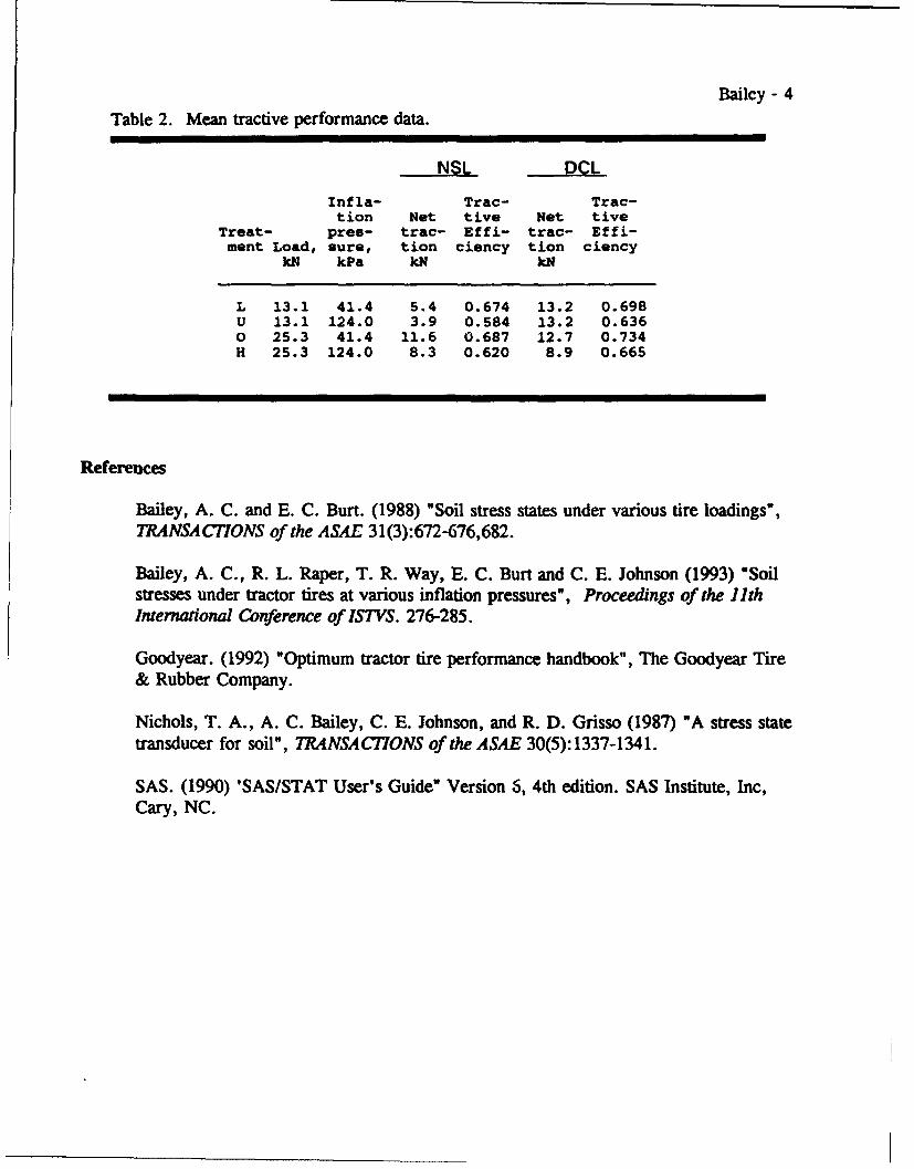
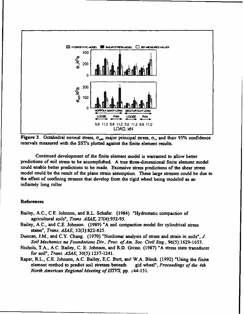
Soil Stresses Under Tractor Tires, A. C. Bailey, R. L. Raper, Ao0ession ForC. E. Johnson, T. R. Way, and E. C. Burt NTIS GRA&I
DTI C TAR fJ
Soil Compaction Research Needs, P. T. Corcoran Unanrf•e'Jn~d LI
Localized Energy Dissipation in Strained Granular Materials,Peter K. Haff Distribution/
A Case for Improved Soil Models in Tracked Machine Simulation, Availability CodesF. B. Huck Vail and/orDist Spec ial
Prediction of Soil Compaction Behavior, Clarence E. Johnson,Alvin C. Bailey, and Randy L Raper
iii
Finite Element Modeling of Wheel Performance and Soil Reactionand Deformation, Clarence E. Johnson, Winfred A. Foster, Jr.,Sally Shoop. and Randy L Raper
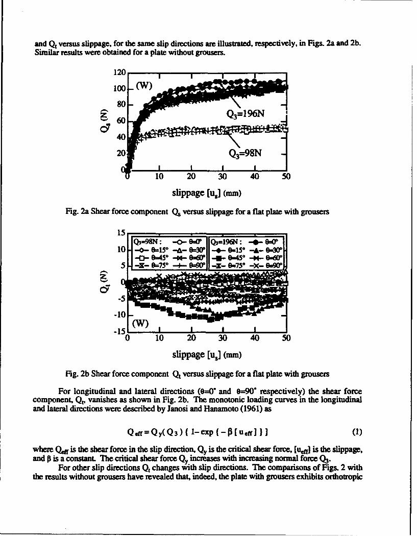
Generalized Janosi's Shear Stress-Slippage Relation, HidenoriMurakami and Tatsunori Katahira
Modeling the Mechanics of Off-Road Mobility Workshop, Mark D.Osborne
Using the Finite Element Method to Predict Soil Stresses Beneatha Rigid Wheel, R. L Raper, C. E. Johnson, A. C. Bailey, andE. C. Burt
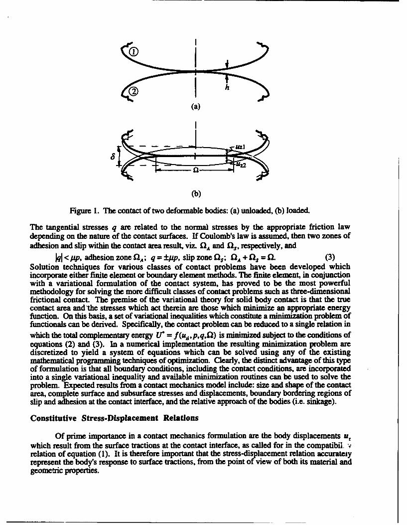
A Contact Mechanics Approach to the Modeling of DynamicSoil-Vehicle Interaction, Antoinette Tordesillas
Tire-Terrain Modeling for Deformable Terrain, Sally Shoop
The Role of High Resolution Simulations in Vehicle PerformanceAssessment, Roger A. Wehage
Soil Plowing Using the Discrete Element Method, David A. Homer
Appendix C: List of Participants ............................. CI
SF 298
iv
Preface
The First North American Workshop on Modeling the Mechanics ofOff-Road Mobility was held 5 and 6 May 1994 at the U.S. Army EngineerWaterways Experiment Station (WES) in Vicksburg, Mississippi. Theworkshop was sponsored by the U.S. Army Research Office under theTerrestrial Science Program of the Engineering and Environmental SciencesDivision.
The idea for this workshop originated with Mr. David A. Homer, MobilitySystems Division (MSD), Geotechnical Laboratory (GL). The workshop wassubsequently organized by Mr. Roger W. Meier, MSD, under the generalsupervision of Mr. Newell R. Murphy, Chief, MSD, and Dr. William F.Marcuson, III, Chief, GL. This report, which documents the proceedings ofthe woikshop, was edited by Messrs. Meier and Homer with the assistance ofMr. Jody Priddy, MSD. Mr. Meier wrote the introduction and workshopsummary in Chapter 1. Ms. Sally Shoop, U.S. Army Cold Regions Researchand Engineering Laboratory, provided the synopsis of the plenary discussionsin Chapter 2.
The workshop organizers wish to thank Drs. Peter Haff, Duke University,Shrini Upadhyaya, University of California at Davis, and Paul Corcoran,Caterpillar, Inc., for serving as working group chairmen and providing us withsynopses of their group's discussions.
Dr. Robert W. Whalin was Director of WES during the preparation andpublication of this report. COL Bruce K. Howard, EN, was Commander.
The contents of this report are not to be used for advertising, publication.or promotional purposes. Citmaon of trade names does not constitute anofficial endorsement or approval of the use of such commercial products.
V
1 Introduction
Background
In the current atmosphere of belt-tightening and streamlining, the Armyneeds a means of assessing the mobility performance capabilities of candidatenext-generation vehicles without first spending tens of millions of dollarsbuilding vehicle prototypes. Shortcomings and design flaws that compromisemobility performance must be identified before they are incorporated into theprototypes at Army expense.
The task of evaluating the mobility performance of vehicles in currentlyaccomplished in part with the NATO Reference Mobility Model (NRMM).1NRMM uses a collection of algorithms, numerics, and empirical relationshipsto forecast maximum steady-state vehicle speed as a function of driver,vehicle, weather, and terrain characteristics. The empirical relationshipsembody more than 40 years of vehicle mobility research, testing, andevaluation. Efforts to improve NRMM and expand its empirical databasecontinue to this day.
There are, however, advances in vehicle design on the horizon that willproduce vehicles that operate outside the limits of NRMM's empiricaldatabase. Many of these concepts-such as central tire inflation systems,rubber belt traction elements, active suspensions, and weight-saving reactivearmor-are already appearing in production and demonstration vehicles. Otherconcepts-such as lightweight-composites and appliqu6 armor, zero-groundpressure running gear, and electric drive technologies-are just around thecomer.' In many cases, the performance characteristics of these vehiclessimply cannot be described within the bounds of the existing NRMM database.Expanding NRMM's empirical database to include these advanced vehicleswould involve extensive mobility field tests on prototype vehicles. This isexactly the type of expense that the Army can no longer afford.
SRichard Ahlvin and Peter Haley. 1992. "NATO Mobility Model Edition 11. NRMM II User's Guide."Technical Report GL-92-19. U.S. Army Engineer Waterways Experiment Station. Vicksburg. MS.
2 Board on Army Science and Technology. 1992. "STAR 21: Strategic Technologies for the Army of the
Twenty-First Century. Mobility Systems." National Academy Press. Washington, DC.
Chapter 1 Introduction
To accurately access future vehicle performance characteristics in theabsence of costly prototyping and field testing, the Army must develop anability to perform virtual mobility testing--the simulation of vehicle mobilityperformance in the computer. This will require advances in the numericalmodeling of vehicle dynamics and vehicle-terrain interaction and in thecharacterization of the terrain for modeling purposes.
In order to 1) assess the current state of the art in vehicle mobilitymodeling, 2) identify the most promising areas of current research, and 3)determine the most profitable directions for future research, the MobilitySystems Division of the U.S. Army Engineer Waterways Experiment Station(WES) invited recognized leaders in the field of vehicle mobility modelingfrom throughout the United States and Canada to participate in a two-dayworkshop on "Modeling the Mechanics of Off-Road Mobility." This reportdocuments the proceedings of that workshop.
Workshop Summary
Prior to the workshop, participants were asked to provide a brief (3-4 page)technical note or extended abstract describing their current mobility modelingresearch efforts. These submissions, which are reproduced in this report, wereassembled into a workshop preprint volume that was provided to all of theparticipants when they arrived at the workshop site. The technical notes wereused by the workshop organizer to determine the interests of each participantin order to assign them to individual working groups. The preprint volumealso served to "introduce" participants to one another. Because the participantscame from a wide variety of organizations and had a wide variety ofbackgrounds, not all of them knew each other or were familiar with eachother's research work. It was hoped that the preprint would help initiate off-line discussions between researchers that might lead to fruitful collaborations.
The workshop began with a brief welcome by the Commander and theDirector of WES and opening remarks by the workshop organizer. These werefollowed by two keynote speeches, which are included here. The first speech,by Prof. J. Y. Wong from Carleton University in Ontario, Canada, addressedthe state-of-the-art in the analytical modeling of steady-state off-road mobilityfor wheeled and tracked vehicles. The second, by Dr. Shrini Upadhyaya fromthe University of California at Davis, described his recent research into thebackcalculation of in situ soil properties from field test results using responsesurface methodologies.
The afternoon was spent in a group discussion trying to determine which ofthe existing mobility modeling paradigms did and did not work so we couldbetter determine the areas where additional research was needed. A synopsisof that session, presented in the next chapter, has been provided by the sessionchairperson, Ms. Sally Shoop from the U.S. Army Cold Regions Research and
2 Chapter 1 Introduction
Engineering Laboratory (CRREL). During that group discussion, the lack of
any standardization of in situ tests for ascertaining vehicle mobility was noted.
A small working group broke off from the main group to address that issue.
Mr. George Mason from WES has submitted a synopsis of those discussions.That synopsis is paraphrased here:
Any standardized test for determining in situ soil properties mustaccount for 1) soil layering and heterogeneity, 2) the effects of changes
in moisture content over depth, 3) the loss of strength that results fromremolding, 4) the effects of organic matter such as grass and roots, and5) the critical depth at which soil shear properties will dictate mobility.It must also permit the backcalculation of unique soil properties, unliketests such as the military cone penetration test which can produce thesame test results for many different combinations of soil strengths andcompressibilities.
A standardized test should i) be able to measure changes in strengthwith depth at 5 cm increments, 2) produce shearing patterns thatcorrelate in some way with the width of loaded area of interest (e.g., ofa track pad or a tire contact patch), 3) include a definition of theremoldability of the soil, 4) be capable of rapid measurements in lowsoil strengths, and 5) be transportable to the field.
The plenary session was concluded by recommending that the remainder ofthe workshop be devoted to the identification of specific research needs andthe facilitation of possible cooperative research between the participants.
To that end, the participants were broken up into three working groups ofequal size the next morning. Each group was asked to return two hours laterwith an enumerated list of the five biggest knowledge gaps in vehicle mobility
modeling. They were also asked to address the question: "If those gaps wereto be filled tomorrow, what would it buy us?" The participants were assignedto the different working groups based on perceived similarities in their needsand interests. For example, one group contained most of the researchersmainly interested in ride dynamics. Another group was composed of theresearchers primarily concerned with the mechanics of vehicle/terraininteraction.
In all, 17 different knowledge gaps were identified (two of the groupssubmitted lists with more than five knowledge gaps and several gaps wereidentified by more than one group):
"* need to determine where the existing modeling techniques don't work
"• need to relate soil mechanics properties to intrinsic oil properties
"* need data on the spatial and temporal variability of soils
Chapter 1 Introduction 3
"* need better ways of coping with inhomogeneity
"* need better ways to measure and evaluate soil properties in situ
S., ._d valid, repeatable (standard) characterization of the real world
* need to instrument the soil without affecting its structure
* need to measure and understand dynamic soil properties
• need to measure soil adhesion and understand its role in mobility
* need to estimate changes in soil resulting from vehicle traffic
* need an adequate effective stress theory for multi-phase media
* need to understand the mechanics of continuous (large strain) failure
"* need to better understand the correlation between slip and sinkage
"* need to predict interface stresses during acceleration and braking
"* need to determine the 3-D response of terrain to vehicle steering
"* need a good model for RAMD prediction
"* need numerical models or lookup tables to speed model execution
If those knowledge gaps were filled, the following could be accomplished:
"* real time simulation of vehicle mobility
"* validation of existing and new mechanisms and models
"* accurate modeling of vehicle agility/maneuverability
"• the ability to predict, design for, and control soil compaction
"* the ability to predict the effects of tread and grouser design
"* prediction of site-specific vehicle mobility (e.g., virtual test course)
"* prediction of vehicle failure and estimates of reliability
"• enhanced mobility-based design and procurement
There are far fewer "knowledge uses" than there are knowledge gapsbecause many of the participants had very similar needs and desires and some
4 Chapter 1 Introduction
of those needs could only be met if several knowledge gaps were filled. It issomewhat surprising that there were almost as many knowledge gaps (17) asthere were participants (22) despite the similarity in their knowledge needs.Perhaps that is a strong indication that there is still much work to be done inunderstanding and modeling the mechanics of off-road mobility.
Despite the lack of consensus as to our most pressing research needs, theworkshop was successful in that it served to let everyone working in the fieldknow where they sand as a group. The current state of the art was illustrated,ongoing research was brought to light and discussed, and knowledge gap:. thatneed to be filled through future research were identified. This was especiallyimportant for the several participants, invited at the behest of ARO, whosebackgrounds were outside the realm of vehicle mobility modeling. Thoseresearchers proposed some inventive new approaches to mobility modeling.Several of those approaches are currently being investigated and will probablylead to research contracts or cooperative research agreements. If nothing elsewere to come of this workshop, that alone will have made it worthwhile.
At the end of the workshup, there was unanimous agreement that theworkshop should become a recurring event. ARO has agreed, in principle, tosponsor a recurring workshop. The Mobility Systems Division of WES hasagreed to host it again. That "Second North American WorKshop on Modelingthe Mechanics of Off-Road Mobility" is tentatively scheduled for August 1995.
Chapter 1 Introduction 5
2 Plenary Discussions
This plenary session was loosely structured with the broad objectives ofconcentrating on identifying the knowledge gaps in the current state ofmodeling vehicle-terrain interaction. Because we were of very diversebackgrounds, and with a wide variety of applications for such modeling, thediscussion began by grouping the applications as those dealing with predictionand improvement of performance (such as vehicle, tire, track, compactor, andagricultural tools), and those dealing with the resulting soil deformation (suchas compaction, mass flow, and terrain damage).
The discussion then focused on the general needs of vehicle-terrain models,as follows:
" The need to relate remotely-sensed mapped parameters to soilparameters and vehicle performance models.
" The need to use FEM (or other sophisticated tools) to generate lookuptables for bigger, virtual reality type models which must run in realtime.
" The need for a common or standard measurement device, and/or a"standard" piece of ground to validate soil devices and models. Thegeneral consensus was for coming up with a "standard" shear device.
"* It was generally agreed that although the vehicle input needed for suchmodels is well defined and understood, the soils characterization andmodeling has a long way to go.
At this point, a small group split off to discuss the device standardizationissue. The remaining participants discussed the following issues regarding thespecific capabilities that are lacking to do the above. Some of this discussioncontinued the second d0y.
The 3-D contact between the driving element and the soil is not oftenknown but must be used as input for rigorous numerical modeling.(However, using contact mechanics, it is the material properties thatmust be well known and the contact is calculated.)
6 Chapter 2 Plenary Discu-sions
Is it valid to apply the traditional Janosi's shear equation and Bekker'ssinkage equation for the case of a 3-D soil-tire contact surface?Janosi's equation assumes horizontal shear and Bekker's sinkageassumes vertical (or normal to the loaded surface) deformation.However, the stresses and deformations involved in soil-tire contact ondeformable terrain are not necessarily vertical and horizontal. AsBekker's equation assumes that the pressure is hydrostatic the directionis not critical, however, the asymmetry of the pressure distributionbeneath the wheel causes problems. Janosi's equation is based on theshear and normal forces on the wheel being vertical and tangential andwas intended to be used with the sum of the forces on the wheel.
"* Soil energy absorption terms needed for vehicle dynamics simulations
are lacking.
"* A good description and understanding of slip-sinkage is needed.
"* Description, numerical formulation and modeling methodology fordealing with the rate effects associated with dynamic loading of verywet and saturated soils.
" Problems associated with modeling large deformations are encounteredin FEM. The use of Eulerian FEM codes was discussed, as wereDiscrete Elements and particle theory along with their largecomputational requirements.
"* The ability to describe and model heterogeneous material (such asboulders and roots) is needed.
"* The ability to handle the effects of multiple vehicles, loading andunloading, repetitive loads is needed.
"• A good (constitutive) model for soil under dynamic loads is needed.
"* Money is needed.
A good deal of the remaining discussion centered around tight budgets andwhere to get the funding to develop and implement these projects. Somefunding is available from the Army Research Office (ARO) and some isavailable from government laboratories through their respective Broad AgencyAnnouncements (BAA). Other sources mentioned were ARPA (AdvancedResearch Projects Agency), AFOSR (Air Force Office of Scientific Research),and CPAR (Construction Productivity Advancement Program). The formationof a consortium to integrate the defense and commercial industrial bases is ofincreasing importance and is sponsored through the US Government'sTechnology Reinvestment Project for Dual Use Technologies. CRDA's(Cooperative Research and Development Agreements) can be used to facilitatecooperative research between the government and private industry while
Chapter 2 Plenary Discussions 7
protecting the interests of both. The research of the future will need to includecollaboration between industry, government and academia in order to get thehighest return on shrinking research dollars.
8 Chapter 2 Plenary Discussions
Appendix AKeynote Lectures
Appendix A Keynote Lectures Al
Analytical ModelingKeynote Lecture
A2 Appendix A Keynote Lectures
Computer Simulation Models for Evaluating the
Performance and Design of Tracked and Wheeled Vehicles
J.Y. Wong'
Summary
A series of computer simulation models for performance and design evaluation oftracked vehicles and off-road wheeled vehicles have emerged in the past decade. In contrastwith empirical models developed earlier, they are based on detailed studies of the mechanicsof vehicle-terrain interaction, and take into account all major vehicle design features andterrain characteristics. Thus, they provide a comprehensive and realistic tool for the vehicleengineer to optimize vehicle design and for the procurement manager to evaluate competingvehicle candidates. These models have been gaining increasingly wide acceptance in industryand governmental agencies. For instance, the model NTVPM for tracked vehicles withrelatively short track pitch has been successfully used to assist vehicle manufacturers in thedevelopment of a new generation of high-mobility military vehicles and governmentalagencies in the evaluation of vehicle candidates in Europe, North America and Asia.
Introduction
In the past two decades, a variety of computer simulation models (computer-aidedmethods) for evaluating the mobility of off-road vehicles have emerged. In the early 1970s,to support decision making processes related to the procurement and deployment of militaryvehicles, an empirical model known as the U.S. Army Mobility Model (AMC-71) wasdeveloped. In the mid-1970s, the second generation of this model called AMM-75 was madeavailable (Jurkat, Nuttall, and Haley, 1975). This version of the model forms the basis for thesubsequent development of the NATO Reference Mobility Model (NRMM). NRMM has thecapability, among others, to predict the tractive performance of off-road vehicles overunprepared terrain using empirical relationships. This capability is, however, limited to theprediction of vehicle performance over two types of terrain, namely, fine- and coarse- grainedsoils.
To assist the development and design engineer to optimize the design of off-roadvehicles and the procurement manager to select the appropriate vehicle candidates for a givenmission and operating environment, a series of computer simulation models have beendeveloped under the auspices of Vehicle Systems Development Corporation of Canada, sincethe 1980s. In contrast with empirical models developed earlier, these models are based ondetailed studies of the physical nature of vehicle-terrain interaction and the principles ofapplied mechanics. They take into account all major design features of the vehicle and the
Department of Mechanical and Aerospace Engineering, Carleton University and VehicleSystems Development Corporation, Ottawa, Canada.
-2-
basic characteristics of the terrain.
For performance and design evaluation of vehicle with flexible tracks, such as rubber-belt tracks or link tracks with relatively short track pitch, commonly found in military fightingand logistics vehicles, a model known as NTVPM has been developed (Wong, 1986, 1989,1992a and b, and 1993; Wong and Preston-Thomas, 1986a and 1988). This model is basedon the assumption that this type of track can be idealized as a flexible belt. It has beensuccessfully used to assist manufacturers in the development of new military vehicles andgovernmental agencies in the evaluation of vehicle candidates in Europe, North America andAsia. For instance, this model has been employed to assist Hagglunds Vehicle AB of Swedenin the development of a new generation of high-mobility fighting vehicles (CV 90), in theexamination of the approach to the further improvement of the performance of the all-terraincarrier BV 206, and in the evaluation of competing designs for a proposed main battle tank.Recently, it has been used in the selection of an optimum configuration for a new, high-mobility armoured personnel carrier for a Spanish vehicle manufacturer and in the assessmentof the effects of design modifications on the mobility of a fighting vehicle over tropicalterrain for an Asian firm. It has also been employed in the evaluation of the effects of designchanges on the cross-country mobility of Canada's main battle tank, Leopard Cl, for theCanadian Department of National Defence and in the assessment of the mobility of a varietyof container handling equipment used by the U.S. Marine Corps.
For tracked vehicles with rigid links having relatively long track pitch, commonly usedin agriculture and construction industry, a model known as RTVPM has recently beendeveloped (Gao and Wong, 1993 and 1994; Wong and Gao, 1994). In this model, the trackis considered to be a system of rigid links connected through frictionless pins. The basicfeatures of this model have been verified with available field test data.
For performance and design evaluation of off-road wheeled vehicles, a model knownas NWVPM has been developed (Wong and Preston-Thomas, 1986b). It can be employed inthe evaluation of the overall performance and design of off-road wheeled vehicles, as well asin the selection of tires for cross-country operations. It has been used in the assessment ofthe effects of different types of tire on the mobility of 6 x 6 and 8 x 8 armoured wheeledvehicles for the Canadian Department of National Defence and in the evaluation of themobility of container handling wheeled vehicles used by the U.S. Marine Corps.
In this paper, the basic features and capabilities of these computer simulation modelswill be presented. Experimental validations of these models with field test data will bedescribed. The applications of these models to parametric analysis of vehicle performanceand to the optimization of vehicle design will be demonstrated.
Computer Simulation Model NTVPM for Vehicles with Flexible Tracks
For high-speed tracked vehicles, such as military fighting and logistics vehicles andoff-road transport vehicles, rubber tracks or link tracks with relatively short track pitch arecommonly used. This kind of short-pitch track system typically has a ratio of roadwheeldiameter to track pitch in the range from 4 to 6, a ratio of roadwheel spacing to track pitch in
- 3-
the range of 4 to 7, and a ratio of sprocket pitch diameter to track pitch usually of the orderof 4. The rubber-belt track and the short-pitch link track will be referred to as "flexibletrack" in this paper and they may be idealized as a flexible belt in the analysis of track-terraininteraction.
The computer simulation model NTVPM has been developed for performance anddesign evaluation of tracked vehicles with flexible tracks, under the auspices of VehicleSystems Development Corporation. The model is intended to provide the vehicle designerwith a comprehensive and realistic computer-aided method to optimize vehicle design, and toprovide the procurement manager with a reliable method to evaluate vehicle candidates. Tomeet these objectives, the latest version of the model, known as NTVPM-86, takes intoaccount all major vehicle design parameters, including sprung weight, unsprung weight,location of the centre of gravity, number of roadwheels, location of roadwheels, roadwheeldimensions and spacing, locations of sprocket and idlers, supporting roller arrangements, trackdimensions and geometry, initial track tension, belly (hull) shape, and angles of approach anddeparture of the track system. The longitudinal elasticity of rubber-belt tracks or of linktracks with rubber bushings are taken into consideration. The track longitudinal elasticityaffects the tension distribution in the track and as a result influences the performance of thevehicle to a certain extent over marginal terrain. The characteristics of the independentsuspension of the roadwheels are fully taken into account in the model. Torsion barsuspensions, hydro-pneumatic suspensions with non-linear load-deflection characteristics, andothers can be accommodated in the model. Suspensions characteristics have a significanteffect on vehicle mobility over soft ground. On highly compressible terrain, such as deepsnow, track sinkage may be greater than the ground clearance of the vehicle. If this occurs,the belly (hull) of the vehicle will be in contact with the terrain surface and will support partof the vehicle weight. This will reduce the load carried by the tracks and will adverselyaffect the traction of the vehicle over terrain that exhibits frictional behaviour. Furthermore,belly contact will give rise to an additional drag component - the belly drag. The problem ofbelly contact is of importance to vehicle mobility over marginal terrain, and the characteristicsof belly-terrain interaction have been taken into consideration in the model. Terraincharacteristics, including the pressure-sinkage relation, shear strength, rubber-terrain shearing(for rubber tracks or tracks with rubber pads) and belly-terrain shearing characteristics, andresponses to repetitive normal and shear ioadings, are taken into account in the model.
Basic Approach to the Development of the Model
In developing the model, the track is assumed to be a flexible belt with knownlongitudinal elasticity. The track-roadwheel system used in the analysis is schematicallyshown in Fig. 1. When a tracked vehicle travels over a deformable terrain, the load appliedthrough the track system causes the terrain to deform. The track segments betweenroadwheels take up load, and as a result they deflect and have a form of a curve. The actuallength of the track in contact with the terrain between the front and rear roadwheels increasesin comparison with that when the track rests on a firm ground. This causes a reduction in thesag of the top run of the track and a change in track tension distribution. It should also bepointed out that an element of the terrain beneath the track is first subject to the load appliedby the leading roadwheel. When the leading roadwheel has passed, the load on the terrain
-4-
a
v_
FLEXIBLE TRACK
Figure 1. A flexible track model
LETE SAND
EhUw
0
LET SANDDITEEU
1200.
5 OO
t)
300- PREDICTED- MEASURED
500Figure 2. Comparison of the measured and predicted
pressure distribution under an Mll3A1 on asandy terrain
-5-
element is relieved. Load is reapplied as the second roadwheel rolls over it. A terrainelement under the track is thus subject to repetitive loading. The loading-unloading-reloadingcycle continues until the rear roadwheel of the track system has passed over it. To predictthe normal and shear stress distributions under a moving tracked vehicle, the pressure-sinkagerelation, shearing characteristics, and responses to repetitive normal and shear loadings of theterrain are taken into consideration.
Based on an understanding of the physical nature of the problem, the mechanics oftrack-terrain interaction is analyzed in detail. A set of equations for the equilibrium of theforces and moments acting on the track system are derived. They establish the relationship,etween the shape of the deflected track in contact with the terrain and vehicle designairameters and terrain characteristics. The solutions to this set of equations define the
sinkages of the roadwheels, the inclination of the vehicle, the track tension distribution, andthe track shape in contact with the ground. From these, the normal and shear stressdistributions on the track-terrain interface, and the track motion resistance, belly drag (if thevehicle belly is in contact with the terrain), thrust, drawbar pull, and tractive efficiency of thevehicle as functions of track slip can be determined. For further details of the model, pleaserefer to the references (Wong, 1989 and 1993).
Experimental Validation
The model can be used to predict the performance of single unit and two-unitarticulated tracked vehicles over unprepared terrain. Its basic features have been validatedwith field test data obtaining using various test vehicles, including Ml 13A1, BV202 andBV206, over a variety of unprepared terrains, including mineral terrain, organic terrain(muskeg) and snow-covered terrain. Figures 2 - 4 show a comparison of the measured andpredicted normal pressure distributions under the track pad of an armoured personnel carrierM113A1 over a sandy terrain, a muskeg, and a snow-covered terrain, respectively. Acomparison of the measured and predicted drawbar performance of an Ml 13A1 over the threetypes of terrain is shown in Figs. 5 - 7, respectively. Figure 8 shows a comparison betweenthe measured and predicted drawbar performance of a two-unit, articulated tracked vehicle BV206, over an undisturbed snow. Reasonably close agreements between the measured andpredicted normal pressure distributions and drawbar performance obtained using NTVPM-86confirm the validity of the basic features of the model.
Applications to Parametric Analysis and Design Optimization
NTVPM-86 can be employed to assess the effects of vehicle design parameters onvehicle mobility and the influence of terrain conditions on vehicle performance. The modelcan also be used in design optimization for a given mission and operating environment.
Figure 9 shows the effects of the number of roadwheels and the initial track tension onthe drawbar pull to weight ratio (drawbar pull coefficient) of a reference vehicle with designparameters similar to that of the Ml 13A1 over a deep snow, predicted using the simulationmodel (Wong and Preston-Thomas, 1986a). It can be seen that both the number ofroadwheels and the initial track tension have significant effects on vehicle mobility over soft
-6 -
PETAWAWA MUSKEG A
E
z2 OM 40SLIP 8.50 1
0
_j--�PREDICTED
\j I -MEASURED
Figure 3. Comparison of the measured and predictedpressure distribution under an M113A1on a muskeg
PETA WA WA SNOW A
E _ _ _ _ _ _ _ _ _
9i 25 SLIP =4.80 %l
W 100 I
inW 200-
1 1--- PREDICTED-MEASURED
z 400
Figure 4. Comparison of the measured and predictedpressure distribution under an M113AJ.on a snow
-7-
50 LETE SAND
z
~30-+
z. 40 +++
) 20 ' +MEASURED-- NTVPM- 86
ccS10.+
0 20 40 60 80SLIP,%.
Figure 5. Comparison of the measured and predicteddrawbar performance of an M113AI on asandy terrain
801 PETAWAWA MUSKEG B
Z 60- -
+ I+ MEASURED
< NTVPM-86
20 40 60 80SLIP,"/.
Figure 6. Comparison of the measured and predicteddrawbar performance of an M113A1 on amuskeg
-8-
30, PETAWAWA SNOW Az
2. 5
2-J
1 MEASURED10. NTVPM- 86
0 20 40SLIP, -.
Figure 7. Comparison of the measured and predicteddrawbar performance of an M113A1on a snow
Feeme snow - froaDevanw•
25
20
z 10-#-- Mean + Standard deviation (SD)
• •Predicted (NTVPM-86)
-5 A
0 10 20 30 40 5O 60 70
SUiP
Figure 8. Comparison of the measured and predicteddrawbar performance of a BV 206on a snow
-9-
0.30
0.250.25 5 roadwheels
.• 0.20 - - 6roadwheels8 roadwheels
•. 0.15 00,
.00
e 0.10
0.05
00 0.1 0.2 0.3 0.4 0.5
Initial track tension/weightFigure 9. Effects of the number of roadwheels and
initial track tension on vehicle perfor-mance on a snow
RPC1e Hope Valley Snow
- Standard---6---'2- 53
0
-4 /
(L.
.0 /-
3 ° /10 20 30 40 50 60
Sl ip, %Figure 10. Effects of suspension characteristics
on vehicle performance on a snow
-10 -
ground. For a given (or existing) vehicle, its mobility over marginal terrain can be greatlyimproved by increasing the initial track tension. This research finding obtained usingNTVPM-86 has led to the development of the central initial track tension regulating systemcontrolled by the driver. Over normal terrain, the driver can set the track tension at theregular level. However, wnen traversing marginal terrain is anticipated, the driver can readilyincrease the track tension to an appropriate level to improve vehicle mobility. The centraltrack tension regulating system is analogous to the central tire inflation system for off-roadwheeled vehicles. A central initial track tension regulating system has been developed andinstalled on a new generation of high-mobility armoured vehicles currently in production inSweden.
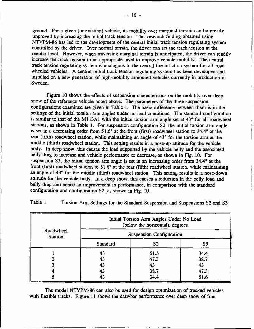
Figure 10 shows the effects of suspension characteristics on the mobility over deepsnow of the reference vehicle noted above. The parameters of the three suspensionconfigurations examined are given in Table 1. The basic difference between them is in thesettings of the initial torsion arm angles under no load conditions. The standard configurationis similar to that of the MI 13AI with the initial torsion arm angle set at 430 for all roadwheelstations, as shown in Table 1. For suspension configuration S2, the initial torsion arm angleis set in a decreasing order from 51.60 at the front (first) roadwheel station to 34.40 at therear (fifth) roadwheel station, while maintaining an angle of 430 for the torsion arm at themiddle (third) roadwheel station. This setting results in a nose-up attitude for the vehiclebody. In deep snow, this causes the load supported by the vehicle belly and the associatedbelly drag to increase and vehicle performance to decrease, as shown in Fig. 10. Forsuspension S3, the initial torsion arm angle is set in an increasing order from 34.4° at thefront (first) roadwheel station to 51.60 at the rear (fifth) roadwheel station, while maintainingan angle of 430 for the middle (third) roadwheel station. This setting results in a nose-downattitude for the vehicle body. In a deep snow, this causes a reduction in the belly load andbelly drag and hence an improvement in performance, in comparison with the standardconfiguration and configuration S2, as shown in Fig. 10.
Table 1. Torsion Arm Settings for the Standard Suspension and Suspensions S2 and 53
Initial Torsion Arm Angles Under No Load(below the horizontal), degrees
The model NTVPM-86 can also be used for design optimization of tracked vehicleswith flexible tracks. Figure 11 shows the drawbar performance over deep snow of four
APC30 - ope Valley Snow
-Standard
25 _-T/W-. 38
o -Canf 1g. R..2 -Config. B.......
0
CL
12 5
8 10 20 30 40 50 soS) ip, %
Figure 11. Comparison of the performance ofvarious vehicle configurationson a snow
a 64 C
RIGD IN TACFigue 12 A igidlin trak mde
- 12-
vehicle configurations, Configurations A and B, the standard configuration with parameterssimilar to that of the Ml 13A 1, and a vehicle configuration similar to the standard one butwith an initial track tension to vehicle weight ratio of 0.3. Configuration A has thesuspension configuration S3 described in Table 1, an initial track tension to vehicle weightratio of 0.25, a track width of 75 cm and a ground clearance of 52 cm. Configuration B hasthe suspension configuration S3, an initial track tension to vehicle weight ratio of 0.3, a trackwidth of 100 cm and a ground clearance of 57 cm. It is shown that Configurations A and Bexhibit superior tractive performance in deep snow over the standard configuration. Thisindicates that NTVPM-86 can be an extremely useful tool for the design engineer to evaluatecompeting vehicle designs and to select the optimum configuration for given operatingrequirements.
Computer Simulation Model RTVPM for Vehicles with Rigid Link Tracks
For low-speed tracked vehicles, such as those used in agriculture and constructionindustry, rigid link tracks with relatively long track pitch are commonly used. This type oftrack system has a ratio of toadwheel diameter to track pitch as low as 1.2 and a ratio ofroadwheel spacing to track pitch typically 1.5.
The computer simulation model RTVPM has been developed for performance anddesign evaluation of tracked vehicles wth rigid link tracks. This model takes into account allmajor design parameters of the vehicle, including vehicle weight, location of the centre ofgravity, number of roadwheels, location of roadwheels, roadwheel dimensions and spacing,locations of sprocket and idlers, supporting roller arrangements, track dimensions andgeometry, initial track tension, and drawbar hitch location. As the track links are consideredto be rigid, the track is assumed to be inextensible. For most low-speed tracked vehicles, theroadwheels are not sprung, and hence considered to be rigidly connected to the track frame.Terrain parameters used in this model are the same as those used in NTVPM.
Basic Approach to the Development of the Model
The model RTVPM treats the track as a system of rigid links connected withfrictionless pin, as shown in Fig. 12. As noted previously, the roadwheels, supporting rollers,and sprocket are assumed to be rigidly attached to the vehicle frame. The centre of the frontidler is, however, assumed to be mounted on a pre-compressed spring.
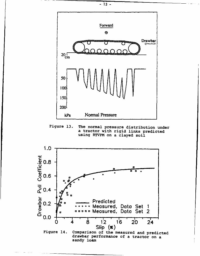
In the analysis, the track system is divided into four sections: the upper run of thetrack supported by rollers; the lower run of the track in contact with the roadwheels and theterrain; the section in contact with the idler; and the section in contact with the sprocket. Byconsidering the equilibrium of various sections of the track system, the interaction betweenthe lower run of the track and the terrain, and the compatibility conditions for various tracksections, a set of equations can be formulated. The solutions to this set of equationsdetermine the sinkage and inclination of the track system, the normal and shear stressdistributions on the track-terrain interface, and the track motion resistance, thrust, drawbarpull, and tractive efficiency of the vehicle as functions of track slip. Figure 13 shows thepredicted normal pressure distribution under a tracked vehicle with seven roadwheels on a
-13-
Forward
Drawbar.-..----
cm
200
50
200L
kPa Normal Pressure
Figure 13. The normal pressure distribution undera tractor with rigid links predictedusing RTVPM on a clayed soil
1.0 -
C0~0.8
0.6 -
0.4- -C-,,o -Predicted"-00 . + + - Measured, Data Set 1
cc I"" Measured, Data Set 20.0 1-4
0 4 8 12 16 20 24Slip (%)
Figure 14. Comparison of the measured and predicteddrawbar performance of a tractor on asandy loam
- 14 -
clayey soil (Wong and Gao, 1994). The detailed description of the model may be found inthe references (Gao and Wong, 1993 and 1994).
Experimental Validation
The basic features of RTVPM have been validated with available field test data.Figures 14 and 15 show a comparison of the measured and predicted drawbar pull coefficientand tractive efficiency as functions of track slip, respectively, for a heavy tracked vehicleused in construction industry. The vehicle has a total weight of 329 kN. It has eightroadwheels of diameter 26 cm on each of the two tracks and the average spacing betweenroadwheels is 34 cm. The track pitch is 21.6 cm and the track width is 50.8 cm. The terrainis a dry, disked sandy loam, with an angle of shearing resistance of 40.1 * and a cohesion of0.55 kPa. The measured data shown in figures are provided by Caterpillar Inc., Peoria,Illinois, U.S.A.
It can be seen that the tractive performance of the vehicle predicted using RTVPM isvery close to the measured one. This suggests that the model is capable of providing realisticpredictions of vehicle performance in the field. It would be desirable, however, to furthervalidate the model over a wider range of terrain conditions.
Applications to Parametric Analysis and Design Optimization
The applications of RTVPM to design evaluation and parametric study of vehicleswith rigid link tracks will be demonstrated through examples.
Figure 16 shows the effects of the track pitch on the drawbar performance on a clayeysoil of a reference vehicle with a total weight of 372.4 kN, predicted using RTVPM (Wongand Gao, 1994). The vehicle has seven roadwheels on each track, a track pitch of 21.6 cm,an initial track tension of 22.30 kN, and a centre of gravity at the mid-point of the trackcontact length. It can be seen that within the range studied, the longer the track pitch, thehigher the tractive performance will be. This is primarily due to the fact that with a longertrack pitch, the normal pressure distribution under the track becomes more favourable. Itshould be noted, however, that with a longer track pitch, the fluctuation in speed and thevibrations of the track system may increase. Consequently, there is a practical limit to thetrack pitch for a given vehicle configuration.
Figure 17 shows the effects of the number of roadwheels on the drawbar performanceof the reference vehicle on the clayey soil. It can be seen that increasing the number ofroadwheels enhances the tractive performance of the vehicle. The improvement in tractiveperformance with a larger number of roadwheels is due to a more uniform normal pressuredistribution.
The model can also be used for design optimization of tracked vehicles with rigid linktracks. Figure 18 shows a comparison of the drawbar performance of the reference vehicleand an optimized configuration (Configuration A) on the clayey soil. Configuration A hasnine roadwheels on each track, a track pitch of 23 cm, an initial track tension of 89.20 kN,
-15 -
100-
S80- ÷4 +÷
Uc 60-+
,, -40-
- PredictedS20.... Measured, Data Set 10000 -Measured, Data Set 2
0 4 8 12 16 20 24Slip (z)
Figure 15. Comparison of the measured and predictedtractive efficiency of a tractor on asandy loam
0.2
.-,C
0
00.1
n - Pitch = 21.6 cmo/: - -Pitch = 17.0 cm
Pitch = 19.0 cmS...... . Pitch = 23.0 cm
0 10 20 30 40
Slip (z)Figure 16. Effects of track pitch on the performance
Slip (S)Figure 17. Effects of the number of roadwheels on the
performance of a tractor on a clayey soil
0.2-
0
00.1
.
o0. _
.0-- Baseline°• i ....... Configuration A
0 10 20 30 40Slip (•)
Figure 18. Comparison of the performance of differenttractor configurations on a clayey soil
-17-
and a centre of gravity at 40 cm ahead of the mid-point of the track contact length. It showsthat RTVPM can be a useful tool for the vehicle designer to select the optimum vehicleconfiguration and design parameters,
Computer Simulation Model NWVPM for Off-Road Wheeled Vehicles
NWVPM has been developed for the evaluation of the overall performance and designof off-road wheeled vehicles over unprepared terrain, as well as for the selection of tires forcross-country operations. The model takes into account all major design parameters of thevehicle as well as the tire. The vehicle design parameters considered include: vehicle weight,axle load, axle spacing, location of the centre of gravity, axle suspension stiffness, function ofthe axle (driven or non-driven), axle clearance, track of the axle, belly (hull) shape, anddrawbar hitch location. The tire parameters considered include: outside diameter, treadwidth, section height, lug area/carcass area, lug height, lug width, inflation pressure, averageground contact pressure, and tire construction (radial or bias). Terrain parameters used in themodel are the same as those used in NTVPM and RTVPM.
Basic Approach to the Development of the Model
The model NWVPM consists of two sub-models, one is the tire sub-model and theother is the vehicle sub-model.
The tire sub-model used is that developed by Wong (Wong, 1989 and 1993). Basedon the dimensions of the tire, the inflation pressure and carcass stiffness (or alternatively theaverage contact pressure on a hard surface), the normal load, and terrain characteristics, theoperating mode of the tire ("rigid" or "elastic") is first predicted. Based on a detailed analysisof the mechanics of tire-terrain interaction, a set of equations for the equilibrium of the tirecan then be established. The solutions to this set of equations determine the normal and shearstress distributions on the tire-terrain interface, the motion resistance, (including the internalresistance of the tire), thrust, and sinkage of the tire. A schematic of the tire sub-model usedis shown in Fig. 19.
The tire sub-model is incorporated into the vehicle sub-model to provide a completeframework for performance and design evaluation of off-road wheeled vehicles. The vehiclesub-model takes into account the dynamic inter-axle load transfer and the suspension stiffnessof the axles. Any number of axles can be accommodated. When the track of the front(preceding) axle is the same as that of the rear (following) axle, the tires on the rear axle runin the ruts formed by the tires on the front axle. Terrain properties in the rut will be differentfrom those in the virgin state. To take into account this "multipass" effect, the responses ofthe terrain to repetitive normal and shear loadings are taken into consideration in the model.In addition, both single and dual tires can be accommodated. The output of the modelincludes the load, sinkage, motion resistance and thrust of the axles, and the drawbar pull andtractive efficiency of the vehicle as functions of wheel slip.
The basic features of the model have been verified with available field test data.Figures 20 and 21 show a comparison of the measured and predicted drawbar performance ofa tractor obtained using NWVPM on a plowed and stubble field, respectively.
-18-
RUBBER -TERRAIN, 2 SHEARING
P6at INTERNAL SHEARINGOF TERRAIN
Figure 19. A tire model
PLOUGHED FIELD
z 0
eas4- S• MEASURED
m• • PREDICTED
0 20 40 60 80 100
SLIP (%)
Figure 20. Comparison of the measured and predictedperformance of a wheeled tractor on aplowed field
- 19-
STUBB3LE FIELD
Oh MEASURE-DPREDICTED
0 2
S LIP( % 10 0F'igure 21.. COMParisn SLIP e
perfomanoe Of ah measured
OnnPeicea s t u b b l e f i e l de 1 ed ~P e d c e
ý.O MEDIUM SoIlt
0
10
Fiue2.EfcsSLIP, % 60o8Fig~~ 2. ffe ts Of inflation Pressure on thedrawbar Performance
of-a aw-alwheeled vehicle On a medium soil
- 20 -
Applications to Parametric Analysis and Design Optimization
The applications of NWVPM to parametric analysis of the performance and design ofoff-road wheeled vehicles and to the selection of tires for a given operating environment willbe illustrated through examples.
Figure 22 shows the effects of tire design and inflation pressures of the front and reartires on the tractive performance of a two-axle vehicle on a medium soil, predicted usingNWVPM. The first and second numbers in the inflation pressure combinations shown in thefigure represent the inflation pressure of the front tires and that of the rear tires, respectively.The effects of the static load distribution between the front and rear axles on the drawbarperformance of the two-axle vehicle are shown in Fig. 23. It indicates that because of the"multipass" effect, a lighter static load on the front and a heavier static load on the rear willgive improved tractive performance on the medium soil (Wong, 1989).
Concluding Remarks
Computer simulation models based on empirical relations have played a useful role inthe past. However, with an improved understanding of the physical nature of vehicle-terraininteraction and of terrain response to vehicular loading, a new generation of computersimulation models has emerged over the past decade. They are based on detailed analyses ofthe mechanics of vehicle-terrain interaction and take into account all major vehicle designfeatures and terrain characteristics. These comprehensive and realistic computer simulationmodels have played and will continue to play an increasingly important role in the futuredevelopment of off-road vehicles. For instance, the computer simulation model NTVPM forvehicles with flexible tracks have been successfully used to assist vehicle manufacturers in thedevelopment of new products and governmental agencies in the evaluation of vehiclecandidates in Europe, North America and Asia.
To further develop computer simulation models (computer-aided methods) forperformance and design evaluation of off-road vehicles, the following guidelines aresuggested.
a) It should be clear that the objective of a model is to provide a framework that willenable the engineering practitioner to reaL-,.Ically evaluate the performance or designof off-road vehicles under a variety of operating environments. The development ofthe model is an engineering endeavour and not an academic exercise.
b) The model should address the needs of the vehicle user, designer, or procurementmanager and not that of the theoretician.
c) The model should be developed and implemented in such a manner that will beconducive to practical results and should appeal to a wide spectrum of engineeringpractitioners.
- 21 -
30 12.5/75R20 TIRE, 379-379 kPa
25 MEDIUM SOILW 25 e-e g•e•e
U .
15.)
10. WEIGHT DISTRIBUTION
cc- 39.23 - 33.33 kN- 33.33 - 39.23 kN
0 20 40 60 80SLIP, %
Figure 23. Effects of static weight distributionon the performance of a two-axlewheeled vehicle on a medium soil
d) In the development of the model, including the characterization of terrain behaviour, apragmatic engineering approach should be followed. It should not be unduly dwellingon theoretical niceties.
e) An off-road vehicle is a complex mechanical system. In the development of themodel, emphasis should be placed on an adequate representation of the vehicle, so thatmeaningful results can be obtained to guide its development, design and procurement.
f) While an understanding of the mechanical behaviour of the terrain (soil) is essential,the development of the model is not an exercise in soil mechanics.
g) The success or failure of a model is eventually judged by the market place or by the
engineering practitioner, and not by the theoretician or the bureaucrat.
Acknowledgements
The provision of field test data by Caterpillar Inc., Peoria, U.S.A., for the validation ofthe computer simulation model RTVPM is appreciated. This does not imply, however, thatthe views expressed in this presentation necessarily represent those of Caterpillar Inc.
- 22 -
References
Jurkat, M.P., Nuttall, C.J. and Haley, P.W. (1975), "The U.S. Army Mobility Model (AMM-75)," Proceedings of the 5th International Conference of the International Society for Terrain-Vehicle Systems, Vol. IV, pp. 1-48.
Wong, J.Y. (1986), "Computer-Aided Analysis of the Effects of Design Parameters onPerformance of Tracked Vehicles," Journal of Terramechanics, Vol. 23, No. 2, pp. 95-124.
Wong, J.Y. (1989), Terramechanics and Off-Road Vehicles, Elsevier Science Publishers, B.V.,Amsterdam, the Netherlands.
Wong, J.Y. (1992a), "Optimization of the Tractive Performance of Articulated Vehicles Usingan Advanced Computer Simulation Model," Proceedings of the Institution of MechanicalEngineers, Part D, Journal of Automobile Engineering, Vol. 206, No. DI, pp. 29-45.
Wong, J.Y. (1992b), "Computer-Aided Methods for Optimization of the Mobility of Single-Unit and Two-Unit Articulated Tracked Vehicles," Journal of Terramechanics, Vol. 29, No.4/5, pp. 395-421.
Wong, J.Y. (1993), Theory of Ground Vehicles, John Wiley, New York.
Gao, Y. and Wong, J.Y. (1993), "A Computer-Aided Method for Design and PerformanceEvaluation of Vehicles with Rigid Link Tracks," Proceedings of the 1 th InternationalConference of the International Society for Terrain-Vehicle Systems, Vol. I, pp. 76-85.
Gao, Y. and Wong, J.Y. (1994), "The Development and Validation of a Computer-AidedMethod for Design Evaluation of Tracked Vehicles with Rigid Links," Proceedings of theInstitution of Mechanical Engineers, Part D, Journal of Automobile Engineering, Vol. 208 (inpress).
Wong, J.Y. and Preston-Thomas, J. (1986a), "Parametric Analysis of Tracked VehiclePerformance Using an Advanced Computer Simulation Model," Proceedings of the Institutionof Mechanical Engineers, Part D, Transport Engineering, Vol. 200, No. D2, pp. 101-114.
Wong, J.Y. and Preston-Thomas, J. (1986b), "Development of Vehicle Performance PredictionSoftware," Unpublished Report prepared for the Division of Energy, National ResearchCouncil of Canada.
Wong, J.Y. and Preston-Thomas, J. (1988), "Investigation into the Effects of SuspensionCharacteristics and Design Parameters on the Performance of Tracked Vehicles Using anAdvanced Computer Simulation Model," Proceedings of the Institution of MechanicalEngineers, Part D, Transport Engineering, Vol. 202, No. D3, pp. 143-161.
Wong, J.Y. and Gao, Y. (1994), "Applications of a Computer-Aided Method to ParametricStudy of Tracked Vehicles with Rigid Links," Proceedings of the Institution of MechanicalEngineers, Part D, Journal of Automobile Engineering, Vol. 208 (in press).
Soil Property Determination
Keynote Lecture
Appendix A Keynote Lectures A25
DETERMINATION OF ENGINEERING PROPERTIES OF SOIL IN-SITU
Shrini. K. UpadhyayaProfessor
Department of Biological and Agricultural EngineeringUniversity of California, Davis CA 95616
SUMMARY:
Soil-tire/Soil-track interaction is of particular interest to researchers involved in off-roadmobility and traction research. This includes scientists and engineers involvhd in researchin the field of agriculture, construction, forestry, military, and mining. In agriculture andforestry soil compaction caused by traction devices is also a serious concern. A soundmathematical model is a pre-requisite to obtain a clear understanding of the soil-tire/soil-track interaction process. A key ingredient for any such model is a constitutive relationshipwhich describes the stress-strain behavior of soil. Any suitable constitutive model requiressoil physical properties which describe the elastic behavior of soil, onset of yield andsubsequent plastic flow, material hardening or softening rules etc. Since in-situ soilsseldom behave like remolded laboratory soils or disturbed field samples, it is important to"identify" or "calibrate" the engineering properties of field soil by means of in-situ tests.The technique of obtaining material parameters based on actual system response is knownas "back analysis", "inverse solution", "identification", or "calibration procedure". Forcomplex problems such as soil-traction device interaction where closed form analyticalsolutions do not exist a numerical technique such as a finite element technique iscommomnly used to solve underlying system differential equation. For such cases theback analysis procedure can take one of the two forms: (1) inverse method, and (2) directmethod. This paper addresses the advantages and disadvantages of such techniques, anddiscusses a new technique which overcomes some of their limitations. This new techniqueconsists of developing a so called "response surface" in the parameter space and then usingthis pre-determined surface to "identify" engineering properties of the material based onin-situ tests. Two case studies - (1) a two parameter hypo-elastic model for soil, and (2) acomplex five parameter model for soil which includes nonlinear material behavior in elasticrange, yield based on Drucker-Prager yield criteria and associated plastic flow upon yieldare presented to illustrate the methodology.
INTRODUCTION AND REVIEW OF LITERATURE:
One of the challenges in the design of an off-road vehicle is to equip it with a tractiondevice( tire or track) which can develop high traction efficiently( i.e. optimum tractiveefficiency) while deterring soil compaction. Even an increase of one percentage point inthe tractive efficiency leads to an annual savings of over 100 million liters( about 25 milliongallons) of fuel in U. S. alone[l]. On the other hand, soil compaction has been recognizedas a worldwide problem with serious implications on agricultural sustainability[2].Although, certain amount of soil compaction may even be desirable for some crops undercertain environmental conditions (optimum soil compaction), excessive soil compactioncan lead to diminished soil porosity, reduced water infiltration, increased resistance to rootpenetration, increased tillage energy requirements, decreased biological activity, and areduction in crop yield[3 - 14]. A necessary pre-requisite for the successful design of atraction device is a sound mathematical model for the soil-traction interaction process. Thisinteraction is an extremely complex, dynamic process. A key ingredient of such a model isa constitutive relationship which describes the stress-strain behavior for soil. Schafer et al.
2
[15] stated that an accurate description of soil constitutive relationship is necessary for theintegrity and robustness of the model. Soil is perhaps one of the most complex materialfrom engineering point of view[ 16].
Numerous constitutive models are currently available for soils. Among these are theelasticity models, higher order nonlinear elasticity models, hypo-elasticity models,plasticity models and visco-plasticity models. Desai [16], Desai and Siriwardane [17] andChen and Baladi[18] have discussed these models and their applicability to a specificloading situation in detail. Piece-wise linear elastic models (hyperbola, parabola, splinesand Ramberg-Osgood formulas) tend to be good for a specific loading case but are poor tosimulate general loading conditions. T!igher order nonlinear elasticity models tend toinclude too many parameters and have jimited appeal. Hypo-elasticity models appear toshow some promise. Plasticity models which utilize Von Mises, Mohr-Coulomb andDrucker-Prager failure criteria have been widely used. To include volume changes due toshear in geological materials and also to account for strain hardening or softening behaviorcritical state models have been developed. CAM and CAP models account for growth of theyield surface and have become increasingly popular in civil engineering. Applicability ofcritical state models to unsaturated agricultural soils has been a much debated issue.Hettiaratchi and O' Callaghan[19], Hettiaratchi[20] and Kirby[21] have found that criticalstate concept is applicable to unsaturated soils both qualitatively and quantitatively exceptthat the critical state parameters depend on the soil moisture content. They found that it isreasonable to use total stress in the model(i.e. soil moisture tension can be ignored). Baileyet al.[22] and Bailey and Johnson[ 23] developed a constitutive model for agricultural soilthat relates volumetric strain to octahedral normal and shear stress. This model predictsvolumetric strain of soil samples accurately at limiting values of stresses(i.e. zero and verylarge applied stress). Raper and Erbach[24] and Raper et al.[25] have used this constitutiveequation to compute tangent moduli in a finite element program to predict soil compaction.
All the aforementioned constitutive models require material parameters. These materialproperties describe the elastic behavior of soil, onset of yield and subsequent plastic flow,material hardening or softening rules etc. Typically these parameters are determined usinglaboratory tests. Sometimes remolded soils are employed in the laboratory tests whichmay not behave like field soil. Use of soil properties obtained from remolded samples canoften lead to predictions which are unrealistic and of little value to engineers interested inimproving tire design. Even if field samples are obtained, one of the main problem withthe soil material is that these samples undergo disturbances during excavation and testing,and may not behave like in-situ soil under actual loading conditions in the field. Use ofC ,In penetrometer, grouser plate, and sinkage plate often yield some composite soilpaiameters which depend on the geometry of the test device and loading conditions. Thesecomposite soil parameters are of little use in subsequent model studies based onconstitutive relationship. It is preferable to determine the soil material parameters based onundisturbed in-situ tests. The technique of obtaining material parameters based on actualsystem response is called "back analysis", "inverse solution", "identification", or "calibration procedure". The process of "calibrating" actual field response to modelbehavior is expected to "identify" the material parameters which can accurately predictsystem response in subsequent analysis which utilize the same constitutive model.
The back analysis technique has been successfully used in Geomechanics in studyingtunneling problems in rocks and in investigating settlement problems[26-43]. If a closedform solution exists for the underlying differential equation describing the physicalproblem, then back analysis to obtain the material parameters involves optimizing thedifference between the analytical and experimental responses. However, most real lifeproblems in geomechanics are geometrically and/or materially nonlinear, and an analyticalsolution may not exist. In such cases a numerical procedure such as a finite element
3
method[FEM] may be used to obtain solutions to the governing differential equation.When finite element analysis is used, back analysis may take one of the two forms - 1)inverse method, and 2) direct method.
In the inverse method nodal values of displacements and stresses obtained by a FEMtechnique are used as known boundary conditions and the unknown displacements andstresses are eliminated from the global matrix equation by reduction[41]. A brief discussionof the method is as follows:
Let the FEM result in the following matrix equation:
[K]Iu} = IF} (1)
where K is the global stiffness matrix, u is the nodal displacement vector and F is theglobal forcing vector. Let us partition the global stiffness matrix by collecting all nodes atwhich nodal values are measured in the field as follows:
[Kll K 12 ]J U t_- FIl
K21 K221 U2 J F2 (2)
where u*1 is a vector containing measured nodal values and u2 is a vector containingunknown nodal values. F1 and F2 are known nodal force vectors, and Kij 's [ i= 1,2; j=1,2 ] are partitioned global stiffness matrix elements. Note Kj 's are functions of unknownmaterial parameter vector, p'. Eliminating u2 out through reduction, we get
[K*]{u"} = {F*} (3)where
[K*] = [K11 + K12K- 'K 21]{u*}
{F*} = {F1 - K12K' 21F 2}
In equation (3) only unknowns are pi s contained in the elements of matrix [K*]. Aniterative scheme or a least square optimization scheme can be used to solve equation forunknown material parameters. This inverse technique is quite sensitive to experimentalerror and may not converge at all in some cases[35,40,42]. The direct approach results inmore accurate parameter values. In the direct method, nodal values of the response arecomputed using a finite element method for a set of assumed parameter values. Theseresponses are a function of assumed parameter vector (D), say u(W). The actual values ofresponse at the same nodes can be obtained by field or in-situ tests. If u* is correspondingobserved response to u(p.) then ei=(u*i- u(p)i) is a measure of error in the ith value. A
suitable objective function such as 4=Z ei2 can be optimized using a nonlinear optimizationtechnique[35,40,42]. The direct search methods such as simplex method or its modificationsuch as Rosenbrock's version or gradient based methods such as conjugate gradientmethod or quasi-Newton method can be successfully used depending on the
4
application[26,32,43]. Nodal displacement values are usually better than stress values inparameter identification[32,35,36]. Moreover, it is preferable to map all the parameters tosame range through scaling[32]. Even in the case of simple linear elastic constitutivemodel, the objective function, 0 will be a nonlinear function of material parametervector,& Because of this situation, the objective function, ý may have several localminimas[43]. Therefore, the optimal solution may be sensitive to initial guess values.Sometimes different combination of two or more parameters may lead to sameresponse[non-unique solution][43]. More than one type of test or tests using differentgeometry and/ or loads may be helpful in such cases. Bayesian approach and Kalmanfiltering have been found to be helpful in improving the accuracy of results in the presenceof experimental errors[27,33,40]. The direct method can be computationally veryexpensive since at each iteration a new FEM analysis with updated parameter vector(p)needs to be carried out[42].
Rubinstein, Upadhyaya, and Sime[44] proposed a new methodology which utilizedorthogonal regression technique to develop a response surface in the parameter spacebased on an analytical or numerical (such as a finite element analysis) solution to thesystem differential equation. This response surface was used in the optimization step.Their methodology consists of following steps:
1. A response surface is built using an orthogonal regression technique based on ananalytical or numerical solution to the governing differential equation of the system.The response surface will be a function of unknown material parameters.
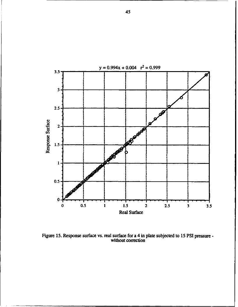
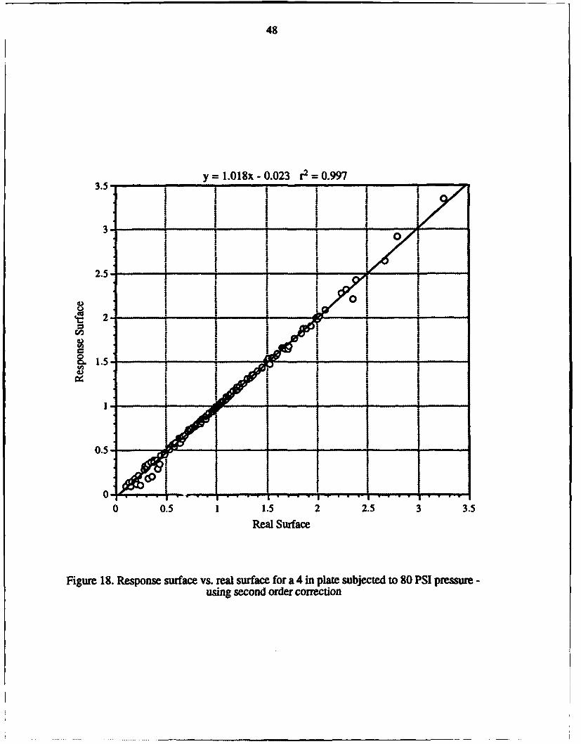
2. This response surface is updated using higher order corrections so that the responsesurface behavior is close to the real surface behavior everywhere in the parameter space.This response surface will be used to predict the response corresponding to theexperimental values(i.e. at the same load and nodal point).
3. Experimental results are transformed such that the real surface and the response surfacewill have one-to-one correspondence everywhere in the region.
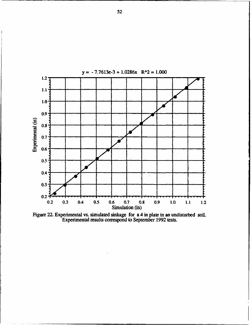
4. Experimental results are optimized against the response surface predictions to obtainmaterial properties of the test material.
The proposed technique is particularly useful in dealing with complex problems whichrequire numerical solution such as a FEM solution to the underlying system differentialequation. The main advantage of this technique is that once the response surface iscreated using an FEM analysis, there is no need to go back to the FEM analysis. In theclassical direct or indirect approach, hundreds or even thousands of time consuming andexpensive FEM evaluations are necessary to determine material parameters throughoptimization technique. In this methodology during the optimization technique only theresponse surface is used to estimate u(p.). This approach is expected to make thistechnique computationally very efficient. These in-situ soil properties can be used insubsequent model studies based on constitutive relationships which utilize these soilparameters. In fact, the methodology is quite general and can be used in other fields toestimate constitutive equation parameters based on in-situ measurements.
5
MATHEMATICAL MODELING
Response Surface Development:
Let us consider a general material constitutive model for soil (or any other material)consisting of m parameters: PlP2,P3,---,Pm For example, if we select a nonlinearconstitutive model with extended Drucker-Prager yield criteria and associated flow rule,then six parameters will be involved[45,46]. These parameters are pl=logarithmic bulkmor 'C; P2= Poisson's ratio, u; p3=yield surface shape factor(i.e. related to the thirdinva&L.,Ia of stress), K; p4=cohesion, c; p5= internal angle of friction, *; P6--initial voidratio, e. The last parameter, e is really related to initial stress condition. The response of asystem to applied load depends on its geometry, material properties and the load itself. Ifthe applied load and the geometry are fixed(i.e. for a given geometry and loading), thesystem response is a function of material constants used in the constitutive equation.There is a function 4D=4 (P1,P2,P3',*.Pm) which represents the system response as thematerial properties used in the constitutive equation are changed. In most real situationsthe differential equation describing the response is nonlinear, this function is seldomknown explicitly. One of the goals of this study is to find an approximate representationfor this real response, 4). This approximation to the real response is termed the responsesurface, F in this study. One convenient way of determining the response surface F is todetermine the variation of F as one of the material parameter, pi is changed while all otherparameters are held constant. Let this response function for the single variable pi be fi(pi).If we repeat this process for each of the m material parameters(i.e. for i=1,2 ....... m), thenone easy way of obtaining the response surface is simply to multiply these componentequations, f(pi), i.e.
SF = Cfl(p)f 2(p2)f3(p3) ..... fm(Pm) (4)
whereF = response surfacefi = a component equation which is a function of parameter pi only.C = constant.Note that this type of solution is often sought in the solution of linear partial differentialequations and is known as separation of variables. For example, in the case of a circularplate placed on a linear elastic medium and subjected to a uniformly distributed load, thereal response, 0 is given on page 350 of Das[47] as
S=l.58qb E (5)
where
4D = the plate sinkage.E = Young's Modulus, E=pl.,u = Poisson's ratio, 'O=P2.q,b = constants (respectively, uniformly distributed load and plate radius).Equation (5) is a multiplication of two functions of the parameters, pl=E and p2---u, i.e.,f1=l/E and f2=(1-u 2). Therefore, in this case the response surface, F can be representedby a multiplication of the component equations as we assumed in equation (4). However,
6
in general such a representation is accurate only in a small region due to geometric and/ormaterial nonlinearities in the system. The error is expected to be small if the range of pi issmall for each of the m parameters.
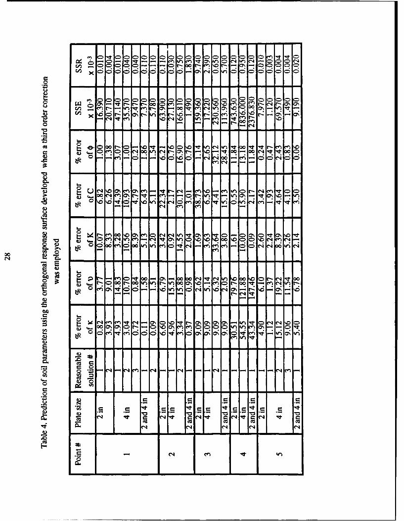
Thus the process of building the response surface requires holding all relevant factorsexcept parameter pi constant(i.e. geometry, loading, all other material properties pj, j= 1,2.... m but j~i) and determining the component equation f(pi). Once all the componentequations are determined, equation (4) can be used to build the response surface. It shouldbe recognized that for each given geometry and loading there will be one response surface.In the case of plate sinkage tests, for a given plate size and load level there will be aresponse surface. Since there are m unknown parameters, at least m field measurementsare needed to solve for these m parameters. In practice, it is preferable to have more than mpoints( i.e. n>m) so that the m parameters can be determined with the help of anoptimization algorithm. Since each unreplicated in-situ measurement corresponds to agiven geometry and loading, each of these experimental values correspond to a point( orcontour) on one response surface. Thus each of the n unreplicated measurements willcorrespond to a point( or contour) on one of the n distinct response surfaces. Note thatmore than one observations at a given geometry and loading refer to the same point (orcontour)on a response surface that corresponds to that geometry and loading. Thusreplicates do not provide additional equations to solve for the parameters, but help incontrolling experimental error. Upadhyaya et al.[48] suggested that at least eight replicatesto adequately deal with the spatial variability in the case of in-situ plate tests. Suppose wehave n distinct combination of geometry and load level there will be n response surfaces,Fi, i=1,2 ..... n. From equation (4) we get
F1 ---Cifilfi2...fim
F2 Cff2...f2m(6)
Fn Cnfnlf.2...f.m
where fij is the component equation corresponding to response i and parameter pj and Ci isthe constant corresponding to the same response surface i.Since each of the material parameter has its own range, some properties such as Poisson'sratio, u vary in a very narrow range (0.0 to 0.5) whereas others such as Young'smodulus, E may vary over a very large range(thousands of kPa). From the point ofoptimization as well as orthogonal regression, it is preferable to map each of the parameterto the same range through scaling[32,49]. Each of the unknown parameter wasnondimensionalized and mapped to vary from -1 to +1 by the following transformation:
2(pi - pi)Pi= (7)
Pi max - Pi mn(n
where:
Pi = nondimensional value of parameter i.Pi = mid point value of parameter i.Pi max = upper bound value of parameter i.Pi mi. = lower bound value of parameter i.
The value of the mid point is zero, upper bound is 1 and the lower bound is -1 for each ofthe nondimensionalized parameter.
Let fi, be the nondimensionalized component equation corresponding to thenondimensionalized parameter p'j and test condition i. The relationship between fij andfij is given by
f fij(8)fPj
whereFj = computed value of the response surface Fi for test i when all the parameters are set
equal to the mid point value of zero.
Moreover, it is convenient if we nondimensionalize the system response to avoid numerical
problems in the analysis. The nondimensionalized response surface is given by:
F'i = C'jf'i2...f'i i=1,2,3,...,n (9)
WhereF'i = nondimensionalized response surface values corresponding to the ith test condition,C'i = correction constant, approximately equal to 1.
The data for the creation of response surfaces can be obtained from any analytical ornumerical models. We propose to use an orthogonal regression technique to determine thecomponent equation fi-. The use of an orthogonal regression technique not only providesan equation to accuratey predict the overall system response, but also provides an accurateestimate of regression parameters[49,50,51]. An accurate estimation of regressionparameters is essential in order to identify the unknown material parameters byoptimization. The function f i. is an orthogonal polynomial of parameter p'j and is givenby:
k
r'~ airp'! 10r=0
The values of ak, ,r=1,2 ....... k are determined by using model response (analytical ornumerical such as FEM) and orthogonal regression techniques. Only requirement for theuse of orthogonal regression in curve fitting is that p'i be equally spaced during modelevaluation while all other material parameters be held at the mid point values. Thetheoretical value of the correction constant, C'1 in equation(9) is one. However, whencurve fitting is employed to determine the regression coefficients,air, the value of thiscorrection constant may be slightly different than one. The actual value of C'j can be foundby a employing linear regression technique between Fi and (f'ijf'i2...f'im). To accomplishthis linear regression, model response at orthogonal points used in building the responsesurface and some additional random points may be used.
Higher Order Correction:
As stated previously, in general the orthogonal response surface is expected to be close tothe true model response only near the mid point and the parameter axes(p'i axis). As we
8
start moving away from the origin or the parameter axes, the two surfaces will depart fromeach other. At large distances from the origin and the parameter axes this error can be
significant. The relation between the nondimensionalized true response, 0%, and theresponse surface, Fi is given by:
4i = F, +(eI0I)
where r, is the error in our approximation ,4'i = Fi.
By assuming that the function ¢", is "well behaved"( i.e. analytic everywhere in theparameter space),this function can be represented in a Taylor series as follows:
where coefficients,bi, bij, bijk, etc. for i=1,2, ...m; j=1,2 .... m; k=l,2 ..... m are
respectively related to the partial derivatives of the function, 0'% with respect to p'i, P'iPj,p'i p'j P'k etc. at the origin(mid point). Equation (12) reduces to f'ij along p'j axis. i.e.
fij = I + bjp'j + bjjp'12 + bp, p73 + ... (13)
Using equations (9), (11), (12) and (13) we get,
ei = dl 2P' I P' 2 +---+ dlmp'lp'm + d23P' 2P' 3 +...+ d2mP'2P'm +-..
where "d" s are constant coefficients related to the cross derivatives of W'i at the origin. Itshould be noted that strictly from a theoretical point of view, an orthogonal responsesurface can be created based on equation (12) rather than equation (9) which relies on theproduct of component equations. In such a case, very little difference is expected betweenthe real surface and orthogonal response surface. If nine equidistant values of each of theparameter p'i, i=1,2 ........ m are used in evaluating real surface, 9m model evaluationswill be needed. If m=2 then 81 model evaluations are needed. On the other hand, if m=6,then an astronomical 531441 model evaluations are necessary. In most real problems,where FEM evaluation of a complex model is necessary, using equation (12) as a basis forthe response surface is infeasible except for the case of a two parameter model. Theresponse surface represented by equation (9) requires only [8*m+l] model evaluations(i.e. for m=2, 17 model evaluations are necessary whereas for m=6, 49 model evaluationsare necessary).
Second Order Correction:
In practice, equation (14) will be truncated at some convenient point. The truncated
function is an approximation to ei and is called the correction function,Ei . If we limitourselves to only the product of the type p'iP'j for i=1,2, ..... m and j=1,2 ..... m, butikj, then E will be a second order function. ITis second order function, E, contains nc inunknowns given by:
9
re(m-l)nc nin 2 (15)
In order to determine the second order correction function, Ei model responses are obtainedat nc additional check points, where nc is greater or equal to nc min. The additional checkpoints can be selected randomly or in a deterministic way. It can be shown that the form ofthe second order correction is:
n-1 M
= e ie (j-1)(2m-j) . k-jp'jp'k
j=1 k=j+l 2 (16)
The "e" coefficients can be derived from a set of nc linear equations with nc min unknowns.A multiple linear regression technique based on equation(16) can be used to estimate the"e" coefficients. Modification to the response surfaces can be accomplished by addingequation (16) to equation (9). The resulting improved response surface is given by:
Fi = Cifijfi2...fim + Ei i=1,2,3,...,n (17)
It is important to emphasize that the second order correction neglects all higher orders ofei. There may be some situations where these higher order corrections are necessary. Insuch cases, it is possible that the second order correction may even give poorer results thannot including any corrections. In situations like these, use of equation (9) may givemore accurate results than equation (17). More discussion on this important issue willfollow when we consider examples.
Third Order Correction:
In order to get more accurate results to the function El. we should consider the higherorder corrections. In this study we will limit ourselves to a third order correction. The thirdorder correction consists of all cross product terms of the parameters upto and includingthe third order terms. The third order function E1 is the summation of ncmi. combination ofcross products, therefore we have n. r. unknown coefficients. It can be shown that thenumber of combinations, n, mi. is given by:
Once again, "e" coefficients can be derived from a set of nc (nc.n,,n) linear equationswith n, j. unknowns. A multiple linear regression technique based on equation (19) canbe used to estimate the "e" coefficients. The modified response surface is given by equation(17).
Estimation of Material Parameters:
Let Uj be one of the n independent experimental observations. In order to make Uiconsistent with F'i, we transform it into a nondimensional value, U'i. The relationbetween Ui and U'i is given by:
U.
U 1i = _- (25)
The subtraction of equation (25) from equation (17) yields a set of n nonlinear equations inm unknowns.
F, - U'l = 0F2 - U'2 = 0
(26)
Fa - U'a = 0
In general equation (26) is seldom an equality due to the presence of approximation as wellas experimental errors. One method of determining engineering properties of the materialinvolves optimizing sum of squares of residuals, SSR defined by:
SSR = min (F'i - U'i)2 (27),i=lI
11
The expression for the SSR in equation(27) is used as an objective function and a nonlinearoptimization technique is used to solve for material parameters. Since F'i is anapproximation to i'i, and Fi can be obtained from equation (9) which corresponds to theoriginal orthogonal response surface or equation (17) which includes higher ordercorrection, we can get different solutions in the vicinity of the real solution depending onwhich expression for Fi is used. The SSR of these solutions is of the same order, thusthe minimum value of the SSR does not necessarily indicate the best solution. Of course,the best solution can be obtained from the sum squares of the residuals which uses O'i inequation (27), i.e.
SSR* = min ({D'i - Ui)2 (28)
Where SSR* is the minimum residuals of the real response surfaces and the test results. Itis recommended to use equation (28) at these different optimum solutions suggested bydifferent versions of F'i to obtain the best results. We will return to this question whenwe consider example problems.
Transformation of Experimental Results:
As explained previously, the accuracy of function F'i may be high in some region on theresponse surface and low In another region. This implies that the estimated parameterswill be high in accuracy sometimes and poor in accuracy some other times. Generallyspeaking, the inaccuracy increases as we move away from the origin and parameter axes.At the origin, the nondimensionalized F'i has a value of unity[cf. eq. (9)]. In some sense,as the values of F'i change from unity the difference between the real and the responsesurface values( both corrected and uncorrected) tend to increase. Thus the values of Fican be used as a measure of this departure. This argument suggests that there exists afunction Vi' =Vi(F'i). Inverse of this transformation, Fi= F'i(Vi) is of particularinterest in our case. This relationship can be used as a transformation rule for experimentalvalues by replacing the real response, 4'i by experimental value, U'i. If we denote thetransformed experimental value which corresponds to F'i by U'i, then we haveU*i=U*i(U'i). The transformation function can be obtained by conducting a polynomialregression between Fi and ('i in some acceptable range, Oi ri. and 4bi ,, thus:
F'-= X i (29)
where "gj" s are regression coefficients. The corresponding transformation rule for theexperimental values is given by:
kU: g u-i (oS= j (30)j--0
12
The value of U*i calculated from equation (30) can be used for replacing Ui in equation(26) and (27). This modification may significantly improve the accuracy of the parametersobtained through optimization. We will explore this aspect in more detail when we considerthe example problems.
COMPUTER IMPLEMENTATION OF THE MODEL:
A FORTRAN program was developed to implement this inverse solution technique toestimate material parameter values. This task involves several steps as shown in figure 1.An interface program is used to transform the analytical or numerical results to a formataccepatable to our inverse solution program. The inverse solution program uses modelresponse (either analytical or numerical such as FEM analysis) for the creation of theorthogonal response surface. Higher order correction are implemented on to thisorthogonal response surface in the next step. Following this expeimental data are inputand a transformation is performed on these data to relate them to response surface points.In the last step, an optimization procedure is carried out to obtain the best estimates of thevalues of material parameters. This program allows for selection of any one of thefollowing optimization subroutines called from IMSL library:
1. Nonlinear least squares techniques,2. Complex algorithm,3. Quasi-Newton method,4. Modified Newton Method,5. Conjugate Gradient Method.
CASE STUDIES:
Two Parameter Model:
A simple two parameter material model is selected to illustrate the main features of thistechnique. A cylindrical bar or soil column under uniaxial compression is considered. Thebar is made of a hypoelastic material with an incremental constitutive law given by(p139,Desai and Siriwardane [17]):
do = (E0 + Elo)de (31)
where E0 and E, are the material parameters of interest in this model, u is axialstress(positive in compression), and e is axial strain. Integration of equation (31) yields:
U = L in Eo (32)
where:
u = deformation of the bar (the contraction).L = length of the undeformed bar.Equation (32) will be used as a basis to build the response surface, Fi. The responsesurface will be developed in the following range of parameters E0 and El:
The nondimensional parameters (equation 7) for this case are:
2(Eo-Eo mid poain) E 2(E 1- E mid E (33)EO am - Eominu n I = El mx - El min
The response at the mid point of the parameters is(i.e. origin):
L mE -° i oi + El d oO)
Fi= E -mid point Point mid pointP i (34)
The nondimensional representation of the real surface is obtained by dividing equation (32)by equation (34). The plot of the nondimensionalized real surface obtained by using anapplied stress of a= 689.5 kPa(100 psi), is given in Fig. 2. The approximation of thesurface without any higher order correction is shown in Fig. 3, and the error of thisapproximation is shown in Fig. 4. The response surface describes the real function withreasonable accuracy except at the comers. The error is particularly high as bothparameters (Eo and E1 ) approach their minimum values. The response surface for this casewhich includes second order correction is:
Fi = f'1(E'o)f'2 (E'd) + ei E'oE', (35)
where f I and f 2 are orthogonal polynomial functions of E'o and E', respectively and eiis second order correction coefficient. The function f'1, f 2 and the coefficient ei werefound as described previously.
The second order correction for this case was obtained by using the edge points, the midpoints of the lower and upper range for each parameter - a total of 16 combinations. Theresponse surface with second order correction is shown in Fig. 5, and the differencebetween the real values and the response surface values is plotted in Fig. 6. The secondorder correction decreases the error in the zones of high error (e.g. in the region near theminimum values of Eo and EI). However, this correction to the response surface increasedthe error in some other regions where the error was negligible previously. The basicassumption of the second order correction is that all higher order(third order and higher)cross products are negligible. In this particular example, the plot of the error shown in Fig.4 indicates a high curvature in a small region [in fact only about 3% region] where bothparameters approach their minimum values. Thus, second order correction does notrepresent the error properly everywhere in the region.
Effect of including the third order correction (TOC) was also examined for thi,, twoparameter case. The form of the third order correction is:
Ei = eilEo El + ei2E2E1 + ei 3E°E2 (36)
Figure 7 shows the effect of including third order correction on the response surface.Inclusion of third order correction further reduces the error in the zone of high error (i.e. inthe 3% region where EO and El values are near or at their minimum). Figure 8 is a plot of
14
error when the third order correction is included. Comparison of this figure with figures 4and 6 shows that although the response surface which includes third order correctionreduces the error in the zone of high error , the error in other regions does not necessarilydecrease. In fact, the error increases slightly in some areas.
In order to determine the material parameters(EO and Ej), seven different resoponsesurfaces were created using seven different applied stresses. The stress values used were344.7 kPa (50 psi), 517.1 kPa (75 psi), 689.5 kPa (100 psi), 861.8 kPa (125 psi),1034.2 kPa (150 psi), 11206.6 kPa (175 psi) and 1379.0 kPa (200 psi). The adequacyof the method is illustrated by 12 examples. Table I lists the parameter values selected forthe simulation purpose. The first set of parameter values are randomly Selected. The othereleven examples are based on parameter values along the diagonal, E'0=E'l. The equation(32) was used to calculate the real response. These values were used instead of theexperimental values in the optimization step. Since there is no experimental error in thiscase, we should, in principle, get exact values of the assumed parameters back. Inaccuracyin the results is solely due to the inadequacy of the response surface. Five different initialguess values of the parameters were considered in the nonlinear optimization process foreach one of these examples. The first initial guess values were the mid point values of theparameters, three others were selected randomly and the fifth one was the exact solution.
The transformation equation was estimated using 50 random points of the real surfaceusing equation (29) as a basis f,. -egression.
Exmpl1: Eo and E1 were selected randomly:
The values of the simulated parameters were: Eo= 5666.1 kPa (821.8 psi) and E1=61.8.The nondimensionalized real function value at an applied pressure of 689.5 kPa (100 psi)is 0.80. The results of optimization are listed in Table 2.
Note that both uncorrected response surface and respose surface with third order correctionresulted very good solutions with negligible errors. However, the second order correctionyielded relatively poorer results. When the transformation based on equation(30) wasemployed, all three correction methods yielded reasonably good results (Table 3).Transformation technique significantly improved the parameter estimation for the case inwhich no correction was employed. This transformation was beneficial in reducing errorfor the second order correction technique also, particularly at low parameter values.However, the transformation technique was not quite as beneficial in the case of the thirdorder correction method. Even in this case the error in estimation of the parameters werereduced slightly. Thus, in general transformation technique leads to more accurateparameter estimation.
It should be noted that this particular s3il model shows large increases in response whenE0 and El values are very small compared to all other values of EO and El. This portionof •.e graph corresponds to only 3% of the parameter range (low values of theparameters). This makes it difficult to generate a response surface which is goodeverywhere in the region. Higher order corrections tend to predict the response better inthis region. In so doing, they become less accurate in other regions - especially at largevalues of the parameters (see Figs. 3 through 8). This is an unusal situation whichresulted in the uncorrected surface to generally estimate parameter valu'-s more accuratelythan when the third order correction was employed along with the transformationtechnique. In a well behaved system (i.e. no singularities or large increases in responsesfor small changes in parameter values) the method which employs third order correction is
15
expected to yield more accurate parameter valves. In fact, even very complicated modelsdo not show such singularities or large changes in a small region as we will see with a fiveparameter Drucker-Prager model described below.
A Five Parameter Nonlinear Elastic Soil Model with Extended DrukerPrager Yield Criteria:
The elasto-plastic constitutive material model with Druker-Prager yield criteria is widelyused in geomechanics[45,46]. We assume that in-situ tests consist of plate penetrationtests using circular plates. Here we will not consider the actual field data. Analysis of thefield data to identify material parameters will be dealt later. We explore the feasibility of theproposed methodology in this example for this fairly complex material model. Acommercial finite element program, ABAQUS was used in this study to obtain modelresponse. The orthogonal response surfaces were built using six parameters rv,K,C,¢and e.
Two plates of diameters 50 mm(2 in.) and 100 mm (4 in.) were simulated, with appliedload ranging from 137.9 kPa( 20 psi) to 1034.2 kPa (150 psi) in increments of 68.9 kPa(10 psi), a total of 14 tests for each plate. A response surface was built for each of thosetests in the following parameter range:
lKmin= 0.01 KCmax= 0.10 Kmidpoint= 0.19 No. of points= 9
A typical plot of the non-dimensional sinkage as a function of non-dimensional values of
parameter Kc for a 100 mm (4 in) plate subjected to 551.6 kPa pressure (80 psi) is shown inFig. 9. Note that all other parameters are held constant at their corresponding midpointvalues. Figures 10 through 14 are similar plots except that the dependent variable has beench..nged to %, K, C, 0, and e respectively. These curves show an extremely good fitbetween the real response curve and the response curve obtained by the orthogonalregression (R2 >0.997 for all cases).
The graph of the real surface versus the orthogonal response surface without anycorrection for a 100 mm (4 in.) plate subjected to an applied load of 103.4 kPa (15 psi)is shown in Fig. 15. This graph consists of 55 orthogonal points and an additional 60random points. Figure 16 is similar to Fig. 15 except that the applied load is 551.6 kPa(80 psi) in this case. When the applied pressur. low, soil deformation is small and thesoil medium behaves similar to elastic materia in fact, in our case soil is modeled asnonlinear elastic but if displacements are small even nonlinear behavior can beapproximated by linear behavior). In this case the real surface and orthogonal surface arealmost identical (Fig. 15). As the load is increased, soil will yield and subsequent plastic
16
flow will take place as per the assumed model. Figure 16 reveals that under high load theorthogonal response surface begins to depart from the real surface when non-dimensionalized displacements are below 0.5 or exceed 1.5. Figures 17 and 18 are similarto figures 15 and 16 except that a second order correction has been added to the orthogonalresponse surface. These figures indicate that there has been only marginal improvements inthese curves (especially Fig. 18). Perhaps a higher order correction is beneficial especiallyat high plate loads. Figures 19 and 20 are similar to figures 15 and 16 (also 17 and 18)respectively, except that a third order correction has also been added to the orthogonalresponse surface. Inclusion of third order correction has resulted in an orthogonalresponse surface which is almost identical to the real surface even at high loads. Thisindicates that an orthogonal response surface with third order correction can be usedreliably to predict the real response without having to resort to FEM analysis.
Parameter Estimation:
Since we are dealing with a nonlinear problem the solution is not necessarily unique.Following recommendations may be used as a guide for selecting the best solution fromseveral optimum solutions resulting from the presence of "local minimums":
1. Discard all solutions that have a significantly high SSR (cf. equation 27).
2. Use more than one geometry (i.e. 50 mm and 100 mm diameter plates) and look foroptimum for each of the geometries and also the combination of all the geometries. Acceptthose solutions which are approximately same in all cases. From a practical point of viewtwo plates will be sufficient.
3. Reject any solution in which more than one parameters hit the bounds of the searchdomain. The probability of more than one parameter hitting the bounds simultaneously islow. If in fact, if this really is the case for several initial guesses, and the above two criteriawill be met.
4. In spite of these steps, if more than one optimal solutions are obtained, we recommendthe use of equation (27) to compute SSR. If the response surface with higher ordercorrections has been properly verified as good (i.e. using figures such as 19 and 20described earlier), then the solution which yields the minimum SSR should be accepted asthe best solution. If possible one could use equation (28) to compute SSR* to provideadditional verification. Although, such an approach is preferable, evaluation of equation(28) requires some limited FEM analysis (i.e. one for each plate for each competingsolution).
To explore the suitability of this method to identify the material parameters of this complexconstitutive equation for soil, we selected five different random sets of parameters andconducted simulation studies to obtain true response. Subsequently, these true responseswere used as inputs into to the response surface methodology to re-predict thoseparameters. Since third order correction (TOC) to the orthogonal response surface appearsto be necessary to obtain reasonable results, we will only explore the situation in whichTOC is added to the orthogonal response surface. We chose five different random sets ofparameter values to be re-predicted using the optimization technique. These random setsof points are as follows:
17
Point #1: K€=0.127 u=O.132 K=0.938 C=19.406 0=26.984 e=0.630
Point #2: ic=0.01 1 =0.343 K=0.61 1 C=16.813 0=31.305 e=0.755
Point #3: K-=0.056 u=O.146 K=0.946 C=16.512 40=28.985 e=1.095
Point #4: xK=0.022 o=0.093 K=0.776 C=13.893 0=41.297 e=1.049
Point #5: xK=0.083 ^o=0.233 K=0.884 C=16.867 0=34.856 e=1.123
The initial guess values selected were the "exact solution", "mid point values" and a set offive randomly selected parameter values listed below:
Point #6: x-=0.356 -u=0.238 K=0.889 C=10.791 0=34.579
Point #7: o=0. 131 u=0.297 K=0.996 C=45.693 0=23.932
Point #8: xK=0.039 u=0.116 K=0.889 C=16.271 0=30.728
Point #9: c=0.1 10 u=0.088 K=0.610 C=20.472 0=23.566
Point #10: ic=0.014 )=0.360 K=0.907 C=16.979 0=23.778
The re-prediction process was carried out using 50 mm (2 in. ) plate, 100 mm (4 in.) plateand a combination of 50 mm (2 in.) and 100 mm (4 in.) plates. For each case we used theexact solution and the mid point as initial guesses. The five randomly selected guess pointswere used only for point # 1 for both plates and also the combination of plates. However,for the 100 mm (4 in. ) plate all seven initial guess values were use to seek the optimumsolution for each of the five random set of parameter values.
The results of this analysis are listed in Table 4. An examination of the results indicatesthat the reasonable solution with minimum SSE usually leads to good solution except for
point #4. Point #4 results in very large errors for both parameters Kc and U. However, anexamination of SSE indicates that none of the solutions is reasonable. Our suspicion is
that for this values of K and A, the soil is extremely hard and deforms very little. Underthese circumstances, the nonlinear elastic model for soil with Drucker-Prager yield criteriais perhaps inappropriate.
DETERMINATION OF IN-SITU SOIL PROPERTIES:
Field tests were conducted during November, 1991 and September, 1992 using ourinstrumented soil-test device in a Yolo loam soil in the vicinity of the U.C. Davis campus.In November 1991 tests were conducted in an undisturbed soil using 50.8 mm (2 in.),76.2 mm (3 in.), 101.6 mm (4 in.), 127 mm (5 in.), and 152.4 mm (6 in.) sinkage plates.When we conducted the field tests we were under the impression that more than onegeometry (plate sizes) were necessary to obtain the engineering properties of soil bytheinverse solution technique. However, later we found that this is not necessarily the
18
case. Even use of one plate size appears to be sufficient. In this study, field test resultsfor 50.8 mm (2") and 101.6 mm (4") plates were only used to determine the engineeringproperties of soil by the inverse solution technique.
Eight replicates were obtained for each plate. Sinkage test data were analyzed usingRecee's approach, i.e.
Table 9 lists the mean values of sinkage coefficients for each of the plate tested. Thevalues of k and n for the 50.8 mm (2") and 101.6 mm(4") plate were used in estimatingmean field response corresponding to a desired pressure for a given plate during theoptimization process to "identify "soil parameters.
Soil shear tests were conducted using two different grouser plates [Plate #1: 203 mm longx 76 mm wide, and Plate #2: 178 mm long x 86 mm wide]. Each plate was tested at twodifferent vertical loads and each test was replicated three times. Grouser plate test resultswere analyzed using the following equation:
=([c+p*tan(ý)](l-e K) (38)
where
T = shear stress, kPac = cohesion, kPap = pressure on the plate, kPaS= soil internal friction anglej = shear deformation, mmK = shear modulus, mm
A nonlinear regression technique was employed to fit the data to equation (38) and obtainshear parameters. Maximum shear stress, Tnax for each test was calculated using thefollowing equation:
Tam = c + p * tan(t) (39)
The analysis of the experimental data resulted in a mean value of cohesion of 11.5 kPaand soil internal friction angle of 32.9 deg. for these tests.
Cone index, bulk density and moisture content data were also obtained in the test site. Eightreplicates of cone index profiles were obtained in the top 152.4 mm (6") layer. The coneindex values were averaged over the depth to get a representative cone index value for eachlocation. Subsequently, all eight replicates were averaged to get a mean cone index valuefor this particular soil condition. Five bulk density and moisture content data were alsoobtained in the test site. Average cone index value was 816 kPa, dry bulk density was
19
1510 kg/m 3, and moisture content was 8.9% (dry basis). The void ratio was 0.755 basedon a particle density of 2650 kg/m3.
During September, 1992 only three sinkage plates were used for sinkage tests. Twodistinct soil conditions ( undisturbed and tilled/loose) were included in these tests. Onceagain eight replicates of sinkage tests were obtained for each plate and analyzed usingequation (37). Sinkage parameters for the undisturbed and tilled soil conditions of theNovember 1992 tests are also listed in Table 5. Once again, the mean sinkage parameterscorresponding to 50.8 mm (2") plate and 101.6 mm (3") plate were used in estimating fieldresponse for identifying Engineering parameters of soil.
Shear test procedure as well as data analysis techniques were similar to the procedureemployed in analyzing the November, 1991 shear tests. The mean value of cohesion forthe undisturbed soil condition was 32.3 kPa, and the internal angle of friction was 27.2deg. The corresponding values for the tilled soil was 22.7 kPa and 22.8 deg.
Moreover, soil bulk density, cone index and moisture content data were also obtained asdescribed for the November 1991 tests. The undisturbed (also referred as firm) soil had amean dry bulk density of 1510 kg/m3, moisture content of 5. 14 % (dry basis), and an voidratio of 0.755. The loose or tilled soil had a dry bulk density of 1433 kg/m3, 4.55 %moisture content (dry basis), and a void ratio of 0.851. The cone index data wereinconsistent and were ignored for these soil conditions.
Table 6 lists the Engineering parameters of soil estimated from the optimization processwhich utilized the orthogonal response surface including the third order correction. Boththe best results based on SSE and SSR, and reasonable results based on our search criteriaare listed in Table 6 for all the three soil conditions. The best estimates of the cohesion andsoil internal friction angle values listed in Table 6 do not agree with the correspondingvalues listed in Table 5, which are grouser shear test results. This agrees with ourhypothesis that the grouser shear test provides geometry dependent soil parameters, butnot the basic soil constitutive property. Only the 101.6 mm (4 in.) plate was used for"identifying" soil parameters through optimization. Figures 21 and 22 show theexperimental and simulated sinkage for a 101.6 mm (4 in.) plate obtained using back-calculated soil parameters for September 1992 tests in an undisturbed soil (firm soil).These results indicate that the estimated soil parameters are very good. However, whenthese same parameters were used to compare the response of a 50.8 mm (2 in.) plate in thesame soil condition poor agreement was found between experimental and simulated sinkage( Figs. 23 ). This plot indicates that the parameters predicted from 101.6 mm (4 in.) platetests are unable (under predict) to predict the behavior of 50.8 mm (2 in.) plate in the field.Similar results were obtained in the other soil conditions tested also. We feel that this is dueto the edge effect which is not included in our model. Use of an interface element at thesoil-plate interface appears to be necessary. Since 101.6 mm (4 in.) plate is lesssusceptible to edge effect compared to the 50.8 mm (2 in.) plate, we feel the parametersestimated from a 101.6 mm (4 in.) plate are more reliable. We recommend using a largediameter plates in futr 7e tests.
CONCLUSIONS
Based on this study we reached the following conclusions:
1) A response surface methodology based on an orthogonal regression in the parameterspace has been developed to "identify" , or "calibrate" engineering properties of anymaterial based on in-situ tests. The orthogonal response surface was created from an
20
analytical or numerical(such as FEM) solution to the underlying differential equation of thesystem which utilizes these engineering properties in a constitutive equation. Atransformation technique was developed to map the model response or experimental data onto the response surface.
2) The proposed methodology worked very well (i.e. very little error) in the case of a twoparameter hypo-elastic model for soil. When the second order correction was included witha transformation of data very small errors resulted in parameter estimation. Inclusion ofthird order correction to the orthogonal response surface reduced the chance of large errorin parameter values.
3) When this technique was used in the presence of random noise, the predictedparameters were found to be insensitive to the noise.
4) When this methodlogy was applied to a complex five parameter model for soil(nonlinear elastic behavior with Drucker-Prager yield criteria and associated plastic flowupon yield), it appeared to work reasonably well. A third order correction to theorthogonal response surface appears to be necessary to obtain reasonably good solution.When both the logarithmic bulk modulus (Kc) and Poisson's ratio (0) are low, soil becomesvery rigid and the methodlogy will not yield a good solution. Under such circumstances,perhaps the soil model chosen is inappropriate.
5) The response surface methodology was successfully employed to "identify"engineering properties of soil based on field tests for different soil conditions in a Yololoam soil. We suspect that edge effect makes the parameter prediction using field datacorresponding to small plates such as 50.8 mm (2 in.) diameter plate inaccurate. Use oflarger plates such as 101.6 mm (4 in.) plate is recommended to reduce this edge effect.Use of Teflon coated plate with beveled edges and slip elements at the plate edge in themodel may also increase the accuracy of parameter prediction.
The proposed methodology has not only applications in geomechanics, but also in otherareas such as biological engineering(plants and animal tissues, food products etc.) wherenon-destructive in-situ tests are the only means of obtaining accurate estimate ofengineering parameters.
ACKNOWLEDGEMENTS
The financial support received from the Goodyear Tire and Rubber Co. and the Bi-National(United States-Israel) Agricultural Research Development [BARD] agency to conduct thisstudy is gratefully acknowledged.
21
REFERENCES
[1] W. R. Gill and G. E. VandenBerg, Soil dynamics in tillage and traction.agriculture Handbook No. 316, U. S. Govt. Printing Office, Washington, D. C. 51 lp.(1968).
[2] S. C. Gupta and R. R. Allmaras, Model to assess the susceptibility of soils toexcessive compaction. In Adv. Sou Sci., Springer Verlag, NY, p 56-100 (1987).
[3] S. C. Gupta and W. E. Larson, Modeling soil mechanical behavior during tillage,IL P. Unger et al.(eds.), Symposium on predicting tillage effects on soil physicalproperties and processes. Am. Soc. Agro., Pub. #44, Madison, WI, p 151-178 (1982).
[4] H. M. Taylor and G. F. Arkin, Root zone modification: Fundamentals andalternatives, In G. F. Arkin and H. M. Taylor(eds.), Modifying the Root Environment toReduce Crop Stress, ASAE Monograph #34, St. Joseph, MI. p 3-19 (1982).
[5] R. Q. Cannel and M. B. Jackson Alleviating aeration stresses, In G. F. Arkin andH. M. Taylor(eds.), Modifying the Root Environment to Reduce Crop Stress, ASAEMonograph #34, St. Joseph, MI. p 141-193 (1982).
[6] W. J. Chancellor , Compaction of soil by agricultural equipment, Div. of Agr.Ser., Univ. Cal., Davis, Bulletin, 53pp (1977).
[7] LAWR - Cooperative Extension, Water penetration in California soils, Tech. Rep.,Joint Infiltration Committee, Dept. of LAWR, Univ. Cal., Davis, Davis, CA (1984).
[8] A. Hadas, D. Wolf and E. Rawitz, Zoning soil compaction and cotton stand undercontrolled traffic operations, ASAE Paper 83- 1042, ASAE St. Joseph, MI 49085 (1983).
[9] A. Hadas, D. Wolf and E. Rawitz, Residual compaction effect on cotton stand andyields, Trans. ASAE 28, 691-696 (1985)[10] A. Hadas, W. E. Larson and R. R. Allmaras, Advances in modeling machine-soil-plant interactions. Soil and Tillage Res. 11,349-372. (1988).
[11] H. D. Bowen, Alleviating mechanical impedance, In G. F. Arkin and H. M.Taylor(eds.), Modifying the Root Environment to Reduce Crop Stress, ASAE Monograph#34, St. Joseph, MI. p 141-193 (1982).
[12] A. Hadas and D. Wolf, Soil aggregates and clod strength dependence on clod sizecultivation and stress load rates, Soil Sci. Soc. Am. J. 43, 1157-1164 (1984).
[13] D. Wolf and A. HadasConventional versus controlled traffic and precision systemfor cotton, ASAE paper 83-1040, ASAE St. Joseph, MI 49085, (1983).
[14] D. Wolf and A. Hadas, Soil compaction effects on cotton emergence, Trans.ASAE, 27,655-659 (1984).
[15] R. L. Schafer, A. C. Bailey, C. E. Johnson and R. L. Raper, A rationale formodeling soil compaction behavior. An engineering mechanics approach, Trans. ASAE,34(4), 1609-1617 (1991).
22
f 16] C. S. Desai, Some aspects of constitutive models for geologic media. Third Int.Conf. on Numerical Methods in GeomechanicsAchen, p2-6, (1979).
[17] C. S. Desai and H. J. Siriwardane, Constitutive laws for engineering materials withemphasis on geologic materials. Prentice Hall Inc., Englewood Cliffs, NJ, 468pp (1984).
[18] W. F. Chen and G. Y. Baladi, Soil plasticity - Theory and implementation,developments in Geotechnical engineering 38, ELSEVIER, NY, 231pp, (1985).
[19] D. R. P. Hettiaratchi and J. R. O' Callaghan, Mechanical behavior of agriculturalsoils. J. Agr. Eng. Res. 25, 239-259 (1980)
[201 D. R. P. Hettiaratchi, A critical state soil mechanics for agricultural soils. Soil useand Management, 3(3), 94-105 (1987).
[21] J. M. Kirby, Measurements of the yield surfaces and critical state of someunsaturated agricultural soils, J. Soil Sci. 40, 167-182 (1989).
[22] A. C. Bailey, C. E. Johnson and R. L. Schafer, Hydrostatic compaction ofagricultural soils. Trans. ASAE, 27(4), 952-955 (1984)
[23] A. C. Bailey and C. E. Johnson, A soil compaction model for cylindrical stressstate. Trans. ASAE. 32(3), 822-825 (1989).
[24] R. L. Raper and D. C. Erbach, Prediction of soil stresses using the finite elementmethod. Trans. ASAE. 33(3):725-730 (1990).
[25] R. L. Raper, C. E. Johnson and A. C. Bailey, Coupling normal and shearingstresses to use in finite element analysis of soil compaction. ASAE Paper No. 90-1086,ASAE, St. Joseph, MI 49085, (1990).
[26] G. Gioda, A numerical procedure for defining the values of soil parametersaffecting consolidation, In.Design Parameters in Geotechnical Engineering, BritishGeotechnical Society London, Proceedings of the 70h European Conference on SoilMechanics and Foundation Engineering, Vol. I, p169-172 (1979)
[27] A. Asaoka and M. Matsuo, Bayesian approach to inverse problem in consolidationand its application to settlement prediction, Third Int. Conference on Numerical Methods inGeomechanics, Aachen, p115-123 (1979)
[28] A. Asaoka and M. Matsuo, an inverse problem approach to settlement prediction,Soils and Foundations, Japanese Society of Soil Mechanics and Foundation Engineering,20(4),53-66 1980
[29] G. Gioda and G. Maier, Direct search solution of an inverse problem inelastoplasticity: Identification of cohesion, friction angle, and in-situ stresses by tunneltests, Int. J. for Numerical Methods in Eng., 15,1823-1848 (1980)
[30] S. Leroueil and F. Tavenas, Pitfalls in back analysis, 10th Conference of Int. Soc.for Soil Mechanics and Foundation Eng., p285-290, (1981).
[31] G. Maier, F. Giannessi and A. Nappi, Indirect identification of yield limits bymathematical programming, Engineering Structures, 4(2), 86-98 (1982)
23
[32] K. Arai, H. Ohta and T. Yasui, Simple optimiLzaon techniques for evaluatingdeformation moduli from field observations, Soils at,•c Foundations, 23(l),107-113(1983).
[331 A. Cividini, G. Maier and Nappi, Parameter estimation of a static Geotechnicalmodel using Baye's approach, Int. J. Rock Mechanics, 20(5), 215-226 (1983)
[34] P. T. Brown and J. B. Burland, Soil parameter evaluation from large scale loadingtests, Symposium InL, Paris, p25-28 (1983)
[35] S. Sakurai and K. Takeuchi, Back analysis of measured displacement of tunnels,Rock Mechanics and Rock Engineering, 16, p173-180 (1983)
[36] K. Arai, H. Ohta and K. Kojima, Estimation of soil parameters based on monitoredmovement of subsoil under consolidation, Soils and Foundations, 24(4), 95-108 (1984)
[37] A. Asaoka and M. Matsuo, An inverse problem approach to multi-dimensionalconsolidation behavior, Soils and Foundations, 2491), 49-62 (1984)
[38] V. U. Nguyen, Back calculations of slope failures by the secant method. SpecialNotes, 34(3), 423-427 (1984)
[39] A. Cividini, G. Gioda and G. Barla, Calibration of geological material model on thebasis of field measurement, Fifth Int. Conference on Numerical methods inGeomechanics, Nagoya, p1621-1627 (1985)
[40] G. Gioda, Some remarks on back analysis and characterization problems ingeomechanics, Fifth Int. Conference in Geomechanics, Nagya, p47-61 (1985)
[ 41] G. Gioda, A. Pandolfi, and A. Cividini, A comparative evaluation of some backalgorithms and their application to in-situ load tests, Second Int. Symposium on FieldMeasurements in Geomechanics, Sakukai(ed.) p 1131-1144 (1988)
[42] A. Anandarajah and D. Agarwal, Computer-aided calibration of a soil plasticitymodel, Int. j. for Numerical and Analytical Methods in Geomechanics, 15, 835-856(1991).
[43] Y. Ichikawa and T. Ohkami, A parameter identification procedure as a dualboundary control problem for linear elastic materials, Soils and Foundations, 3292), 35-44(1992).
[44] D. Rubinstein, S. K.Upadhyaya, and M. Sime. 1994. Determination of in-situproperties of soil using response surface methodology. Accepted for publication in J.Terramechanics.
[45] D. C. Drucker and W. Prager, Soil mechanics and plastic analysis or limit design,Quarterly Appl. Mech., 10, 157-165 (1952).
[46] ABAQUS, Thoery Manual, Version 4.8, Hibbitt, Karlsson and Sorensen, Inc.(1989)
[47] B. M. Das, Evaluation of soil settlement, IILAdvanced soil mechanics, Ch. 6,Hemisphere Publishing Corporation, NY, p339-401 (1983).
24
[48] S. K. Upadhyaya, D. Wulfsohn and J. Mehlschau, An instrumented device toobtain traction related parameters, Accepted for publication in J. Terramechanics, (1992).
[49] G. W. Snedecor and W. G. Cochran, Curvilinear regression, lILStatisticalMethods, Ch. 15, Sixth ed., p447-471 (1967).
[50] J. L. Glancey and S. K. Upadhyaya, A testing procedure for agriculturalimplements, ASAE Paper No. 90-1542, ASAE St. Joseph, MI 49085, (1990).
[51] J. L. Glancey, S. K. Upadhyaya, W. J. Chancellor and J. W. Rumsey, Predictionof implement draft using an instrumented analog tillage tool, ASAE Paper No. 91-1065,ASAE Si Joseph, MI 49085, (1991).
25
Table 1. Parameter values used in the simulation studies
Table 2. Parameter values obtained through optimization for the cases when no correctionwas included as well as the case for which second order and third order correction were
included
Without correction Second order correction Third order correction
No. error error SSE error error SSE error error SSEofEo of E, x10-3 ofEo ofE, xl0-3 ofEo of E, x10-3
Figure 23. Experimental and simulated sinkage for a 2 in plate in an undisturbed soilwhen the soil parameters obtained using the inverse solution technique using a four inchplate test was used to simulate 2 in plate behavior. Experimental results correspond toSeptember 1992 tests.
Appendix BTechnical Notes
Appendix B Technical Notes B1
SOIL STRESSES UNDER TRACTOR TIRES
A.C. Bailey, R.L. Raper, C.E. Johnson, T.R. Way, and E.C. Burt'
Introduction
Soil stress state transducers (SST's) have been used to determine the state of stressbeneath tractor tires operating under a range of dynamic loads and inflation pressures. Thestress state transducer has been described by Nichols et aL.(1987). These SST's provide thedata necessary to calculate the complete stress state at the transducer. The stress state is a 3x 3 symmetric tensor with 6 independent stresses, and may be represented by the 6independent stresses, the three principal stresses (a,, G2, 03) and their directions, or stresseson particular planes, such as the octahedral shearing (t,) and normal (a..) stresses and theirdirections (Bailey and Burt 1988).
Procedure
A recent experiment (Bailey et al. 1993) studied the effect on soil stresses of 4combinations of tire loads and inflation pressures, Table 1. Treatments L and H arecombinations of load and inflation pressures taken from the manufacturer's recommendations(Goodyear 1992). Treatment U (underload, load less than recommendation for the inflationpressure) used the load from the L level (13.1 kN) and the inflation pressure from the Htreatment (124 kPa). Treatment 0 (overload) treatment used the load from the H level (25.3kN) and the inflation pressure of the L treatment (41.4 kPa). The tire was operated at aconstant forward velocity of 0.15 m/s and a constant slip of 10%.
Two soils, Norfolk sandy loam (NSL) and Decatur clay loam (DCL), and two profilesin each soil were used. One profile was relatively loose and uniform. A hardpan waspresent in the second profile. A SST was placed at the depth of the hardpan (hardpan depth)and a second SST placed midway between the surface and the hardpan (shallow depth). BothSST's were aligned directly under the centerline of the path of the tire. Soil bulk densitysamples were taken in each tireprint at the depth of each SST after completion of the tests.
Results and Discussion
Typical data from a SST are shown in figure 1. The data shown are from the Htreatment at the hardpan depth in the NSL with a hardpan. The value of 0 on the distanceaxis represents the horizontal location of the tire axle, and data at positive distances represent
'The authors are: Alvin C. Bailey and Randy Raper, Agricultural Engineers, NationalSoil Dynamics Laboratory, USDA-ARS, Auburn, AL.; Clarence E. Johnson, Professor,Agricultural Engineering Dept., Alabama Agricultural Experiment Station, AuburnUniversity, AL.; and Thomas R. Way, Agricultural Engineer, and Eddie C. Burt, Researchleader, National Soil Dynamics Laboratory, USDA-ARS, Auburn, AL.
Bailey - 2
OTable 1. Mean octahedral stresses at peak oa, from all treatments
NSL DCL
Deep Shallow Deep ShallowInfla- depth depth depth depthtion
Treat- pres-ment Profile Load, sure, owt Ct o~t Ot oCt Tt oct vt
Figure 1. Typical measured pressures from Figure 2. Calculated stresses from datathe stress state transducer under the shown in figure 1.centerline of the tire.
pressures in front of the tire. Figure 2 presents the calculated principal stresses (a,, a,, anda3) and the octahedral stresses (a. and -,,,) for the data from figure 1 using the samedistance axis. The major principal stress, a,, is the greatest stress but displays the sametrends as the octahedral shearing stress. For this discussion the octahedral stresses a,,t and
Bailey - 3
T", will be used to represent the stress state in the soil under the tractor tire. The peak valuesof a., and the corresponding values of x were selected for further analyses. Table 1presents of the means of the 4 replications of o;, and -c, from all treatments, soils, andprofiles.
The peak values of o and the corresponding values of t• were analyzed with SAS(1990) using a factorial design on each soil separately. Replications were nested within soilprofile. The multivariate option MANOVA was also used to analyze both octahedral stressestogether.
Higher levels of either dynamic load or inflation pressure generated higheroctahedral stresses beneath the tractor tire in both soils when averaged across all depths andsoil profiles (figures 3 and 4). Both dynamic load and inflation pressure were significant
150 o 150 I ("oct" I lOct I 'IOct
C" . .
(0100 ( 100
60 - 0-
0 0
50 *" 05
13.1 25.3 13.1 25.3 441.4 124.0 41.4 124.0
NSL DCL NSL DCL
-Dynamic load, kN Inflation pressure, kPa
Figure 3. Effect of dynamic load on Figure 4. Effect of inflation pressure onoctahedral stresses for two soils averaged octahedral stresses for two soils averagedacross profiles and depths. across profiles and depths.
factors (5 % level) affecting the two octahedral stresses, except for inflation pressure on .,, inthe DCL. This exception is probably because the DCL had the greatest variability in -Tr (adeviatoric stress contrasted to a.,, an average stress). Both dynamic load and inflationpressure were significant factors (5% level) affecting the bulk density and increase in bulkdensity at each depth level in each soil.
The mean net traction and tractive efficiency data for all treatments in each soil arepresented in Table 2. An ANOVA of the net traction and tractive efficiency showed thatinflation pressure and dynamic load both had significant effects on both performancevariables, and that higher inflation pressures had lower net traction and tractive efficiencies atthe same dynamic load. These results support the conclusions from the soil stresses and bulkdensity data. Higher inflation pressures at the same dynamic load have lower tractiveefficiencies and generate higher soil stresses and soil compaction.
Bailey - 4Table 2. Mean tractive performance data.
Bailey, A. C. and E. C. Burt. (1988) "Soil stress states under various tire loadings",TRANSACTIONS of the ASAE 31(3): 672-676,682.
Bailey, A. C., R. L. Raper, T. R. Way, E. C. Burt and C. E. Johnson (1993) "Soilstresses under tractor tires at various inflation pressures", Proceedings of the 11thInternational Conference of ISTVS. 276-285.
Nichols, T. A., A. C. Bailey, C. E. Johnson, and R. D. Grisso (1987) "A stress statetransducer for soil", TRANSACTIONS of the ASAE 30(5): 1337-1341.
SAS. (1990) 'SAS/STAT User's Guide" Version 6, 4th edition. SAS Institute, Inc,Cary, NC.
Soil Compaction Research Needs
P. T. Corcoran'
Introduction
There are two needs for compaction research that are potential topics for the workshop on"Modeling the Mechanics of Off-Road Mobility". Those topics are predictive analytical modelsfor machine compaction, and the forecasting of machine compaction performance on specific jobsite conditions.
These two needs are similar in that both are needed to reduce the requirements for machinetesting. Analytical models for machine compaction can reduce the need for expensive prototypetesting, and improve the understanding of relationships between machine and soil in theproduction of compaction. Performance forecasting can eliminate the need for proof testing, andimprove the quality of soil structures.
Analytical Compaction Models
There has long been a need for accurate and complete analytical compaction models. The idealis to have such models based on proven theory, and not be dependent on relationships definedonly by empirical testing. Although empirical testing is often the most attractive as a low riskpractical means to define machine/soil relationships, empirical testing is always inherentlylimited in application to those parameters and ranges of parametric values included in whateverexperiments provide the data base for empirical relationships.
Conversely, theoretically based analytical models are essentially unlimited in range ofapplication. The more complete the theory and the more detailed the model, the broader therange of application. Historically analytical soil compaction models have been limited by a lackof computational capacity and detail to handle the non-linear and fine grained characteristics ofmachine soil compaction problems. These technological hurdles are coming down with thecomputational speeds of modem computer work stations, and the sophistication in newermodeling software.
Recent work with a finite element soil compaction model is confirming the technological hurdlesto a comparatively complete and detailed model are gone or greatly reduced. The challenge nowbecomes one of using this technological opportunity. The author is interested in sharingexperiences with others addressing the need for predictive models, both analytical and empirical.
'Senior Project Engineer, Product Research, Caterpillar Inc.
Compaction Performance ForecastingCompaction is very often a critical need in the construction industry. Achieving compactionspecifications can be the critical path guiding the progress of a construction site, and thereforeachieving compaction specification mi -1e the determinant factor in scheduling and costing ajob. Contractors need accurate inforn on the ability to meet compaction specifications, andtraditionally this has required proof tL *. Proof testing can be far from an accurate means toinsure compaction specifications will actually be met. The common variability in job site soils,virgin soil conditions, and the influence of weather can destroy the accuracy of proof testing.
An ideal would be the ability to forecast the performance of compactior machines based onspecific job site conditions, and adapt machines and operating procedures to the job site asneeded for both maximum efficiency and performance. However, most contractors lackinformation and interpretation to achieve such an ideal.
There appear to be two major needs to allow for the ir-' ,vements of performance forecastingand the reduction of need for proof testing; the quan -t .. . onships between machineparameters, job site conditions, and compaction specificatic-s; and the relationship betweenlaboratory compaction measurement and actual field capabily.
Quantification of relationships between machine, soil, and specifications is perhaps little moredifficult then recording information already available from most job sites t,3 establish a data base.There may be some incremental additional information required, however, it would be c:ntraryto the purpose of performance forecasting to require significant additional information than 'hatnormally available. A requirement for significant additional information would only trade-effone inefficiency for another and thus not bring about a net gain in overall job efficiency. Areasonably inclusive database should then give the opportunity to establish correlations yieldinga forecasting capability.
Improving the relationship between laboratory compaction measurement and actual fieldcapability may be more difficult. The problem is compaction machines in the field do not havethe same energy efficiency nor use the same mechanism to produce soil compaction as standardlaboratory procedures. Therefore, densities achievable in the laboratory are not necessarilyachievable in the field at the same energy level and maybe not at any energy level depending oncompaction equipment available. Additionally, as shown by energy/density relationships fromlaboratory testing, optimum moisture levels vary with compaction energy and may vary withmethod of compaction. The need is to provide information to guide field use of compactionmachines both for the selection of the optimum machine, and the optimum use of the machine.Obtaining such information could require a significant amount of controlled testing and thereforebe a relatively costly endeavor.
One possible alternative to establishing correlation between laboratory and field throughempirical testing would be the development and verification of fundamental theory of soilcompaction. Such a theory may already be in existence based on the compaction energy/densityrelationships defined by current laboratory testing. Therefore, expansion of a theory of this typeto correlation between laboratory energy and actual field energy could become the foundation forperformance forecasting and not require large amounts of machine tests.
There may be a significant amount of compaction forecasting information already available butnot widely disseminated, or there may be a significant amount of information available from awide distribution of sources but not consolidated, or there may simply be a lack of informationpertinent to the need. The author is interested in sharing thoughts and ideas on the need, value,and feasibility for accurate performance forecasting of soil compaction and the availability ofpertinent information.
Localized Energy Dissipation in Strained Granular Materials
Peter K. Haffl
A granular material is a mechanical system composed of distinct macroscopicinteracting components. A soil, a sand dune, a heap of mine tailings, and a fractured rockmass, are all granular materials, with "grain sizes" ranging from microns to meters indiameter. There are two approaches that can be used to model granular systemsquantitatively. A continuum method based upon a partial dkferential equation or a discretemethod that retains specific reference to the particulate nature of the medium.
Continuum models require the existence of an "averaging volume", large comparedto grain sizes, within which the characteristics of individual particles can be replaced byvariables like velocity, density, components of stress, etc. Discrete models on the otherhand retain reference to individual particle identities. In discrete models one can investigate"microscopic" behavior that is lost or obscured in the averaging transition to a continuummodel. One such type of behavior in granular systems is the nature of frictional lossesincurred when the medium is subjected to inelastic strain.
A drawback in using a discrete modeling technique is that the number of discreteparticles that can be handled is limited (thousands to tens of thousands of particles), andhence we can study only a small volume of material at one time, while with a continuummodel we can usually model large volumes. Consequently, discrete techniques are oftenbest used to generate insight into microscopic mechanisms that can help us in interpretationof larger scale modeling, or to help construct constitutive relations for use in continuummodels.
In a granular medium subjected to a given load (a generic prototype of a soil orsimilar granular material subjected to vehicle loading), the stress is distributed throughoutthe medium via grain contacts and fluid pressure forces. For simplicity, we consider hereonly dry, noncohesive materials. As strain develops in the material, compression ofindividual grains occurs at the grain-grain contacts. If the contacts do not slip, and thestrain rate is small, then the strain is generally reversible upon unloading and energy loss iszero. At larger strains, grain contacts can slip. Since the contacting surfaces of earthmaterials are frictional, Coulomb-type losses are incurred, and contact positions do notreturn to their original configurations upon unloading.
Particle dynamics studies of energy dissipation in strained granular material point tothe importance of fluctuations in the stress distribution at grain contacts. These fluctuationscan influence the macroscopic lossiness of the material. When a compressive load isapplied to a granular assembly, the allocation of stress among contacts is determined inlarge measure by the geometric placement of grains. Consider for simplicity a system ofcircular or spherical particles. Each particle has a set of neighboring particles with whom itis in contact. By drawing an imaginary line between the centers of every pair of contactinggrains, we define a stress network. A normal force associated with grain stiffness isassociated with each element in this network, as well as a tangential force due to frictionbetween the contacting grains. The normal force exerted across each element of the networkis a function of the deformation at that contact. If the elastic interaction is modeled by a stiffspring, then the force is a function of the instantaneous compression of the spring. Ingeneral the stresses will be different at each contact, i.e., spring compressions will differ,so that there is a distribution of local stress determined by the details of grain packing.
lDepartment of GeologyDuke UniversityDurham, North Carolina 27708-0230
Small amounts of strain can often be accommodated by reversible compression ofthe elastic springs at the contacts, but large strain must be accompanied by slippage androtation of grains. Wherever slippage takes place, frictional forces will lead to energy loss.Because there is a distribution of normal contact forces, some contacts will slip more easilythan others. If a contact is tightly compressed, so that the normal force is large, then acorrespondingly large local tangential stress is needed at that contact to cause it to fail.Conversely, at a contact where the normal spring is not much compressed, slippage isrelatively easy. The frictional energy lost in a slip event is the product of the tangential forceacting during the slip and the amount of displacement incurred at the contact. Assuming forthe sake of argument equa displacements, the greatest amount of energy lost per slippingcontact is at the strong contacts. Conversely, the smallest amount of energy lost per slipevent is at the weakly compressed contacts.
Particle-dynamics-model simulations of sheared granular materials suggest that forthe system as a whole, most energy is lost at contacts of intermediate strength. The strongcontacts do not slip sufficiently often to dominate the overall energy loss, while the weakcontacts slip often but do not generate enough loss per contact to be the dominant lossmechanism. A consequence of this observation is that the macroscopic rate of energy lossin deformation is not a simple function of the grain-on-grain frictional properties ofindividual grains. The energy loss will usually be less than that expected from a simpleaveraging approach, the magnitude of the effect depending upon the detailed distribution offorces over the stress network. A corollary is that since strong contacts cannot slip easily,clusters of grains with strong contacts between them tend to rotate as a whole, with slip andenergy loss occurring on the periphery of the cluster. As the material strains, the stressnetwork continually adjusts to maintain force balance. Rotating friction-locked clusterseventually unlock as their internal stress-network becomes less well aligned with the overallstress field in the medium. At this point the local stresses readjust, slippage begins to occurwithin the previously rigid cluster, and new clusters spontaneously appear nearby.
The frictional losses and hence the energy absorption of the macroscopic granularmedium depend upon the details of such microscopic mechanisms. By elucidating thesemechanisms, discrete computational models can help to further our understanding of thedynamic response of granular systems such as soils to external loads.
2
A Case for Improved Soil Models in Tracked Machine Simulations
F.B. Huck'
Abstract
A planar, multibody dynamics model of a track-type-tractor was developed to provide ananalytical tool to evaluate alternative new tractor designs and to resolve problems on currentproducts. The model has been applied to studies of track chain vibrations, track/sprocketjumping, sprocket/bushing wear, and the influence of track and undercarriage kinematics onfundamental tractor rigid body vibration mode excitation. Applications of the model in studiesof higher frequency vehicle vibrations associated with ride quality demonstrated the importantinfluence that track/soil interface models have on machine vibration excitation and the need toimprove our capabilities in this area.
Introduction
Earthmoving equipment manufacturers must identify ways to reduce product design anddevelopment time and cost to remain competitive in world markets. Manufacturers increasinglyturn to engineering computer analysis as a time and cost savings methodology to supplement andultimately reduce dependence on their more traditional and costly build and test approach toproduct design and development.
As computers continue to increase in speed and expand in memory capacity, engineeringsoftware functionality grows to quickly fill any vacant memory cell or unused CPU cycle.Performance analysts, as a result, are able to develop increasingly realistic and detailedinterdisciplinary models to simulate the overall dynamic response of the complete earthmovingmachine.
The response of the machine ultimately depends upon the external forces which act uponit. In the case of an earthmoving machine, these include gravitational forces, combustion ofengine fuel, operator interactions, and soil reactions. None of these external influences, with theexception of gravity, is as well understood from an analytical standpoint as it needs to be tomatch the degree of sophistication now attainable in dynamics models of the machine itself. Ofthe three least understood forces, the soil force reaction, though possibly not as analyticallyintractable as the human operator, is the most critically lacking component in most earthmovingmachine per.-ormance models.
'Senior Project Engineer - Research Department - Caterpillar, Inc.
Discussion
The Model
One example of a model that pushed the limits of computing resources and analysissoftware to their limits at the time of its development was a 2- dimensional, pitch plane, multibodydynamics model of a high-drive track-type-tractor. Initiated in the mid 1980's, the model wasdeveloped within the framework of the commercial, rigid multibody dynamics code, DRAM(Chase and Angell 1977). The model (Figures 1 & 2) (Huck, 1987) was unique from previoustracked machine models in that it treated each link in the track chain as a distinct rigid body. Thislevel of model fidelity was required to address the range of questions being asked at the time.
Typical Model Applications
The model was applied primarily to questions related to track chain and undercarriagedynamics or to the influence of track and undercarriage dynamics on fundamental machinevibration modes excitation. In the area of track chain dynamics, the model was used tounderstand the relationship among track pitch, catenary length, track tension, and track speed onthe excitation of transverse vibration modes in the track catenaries.
A second application demonstrated how premature wear develops when out-of-tolerancesprocket teeth segments lead to adverse track bushing and sprocket tooth engagement. A thirdapplication simulated the track/spracket tooth jumping that can occur during rapidforward/reverse directional shifts.
The primary application for the model is to optimize undercarriage component placementin order to minimize the influence of track and undercarriage kinematics on the excitiation of thechassis' fundamental rigid body pitch vibration mode in the 4 to 6 Hz range. If overly excited,this mode can affect dozer controllability during finish grading applications.
Importance of Soil Models
The DRAM tracked machine model incorporates simple representations of soil behaviorto simulate the ground reaction forces that support and propel the machine.
Early versions of these models applied Bekker pressure-sinkage like relationships tosimulate the normal support force acting on each individual track shoe. (Bekker, 1969) Likewise,a model similar to that proposed by Kacigen & Guskov was applied to each track shoe grouser tosimulate the soil shearing forces associated with traction.(Kacigen & Guskov, 1968) Thesemodels are simply nonlinear elastic representations of the soil. There is no coupling between thenormal support and traction force models other than the dependence of the tractive forcegenerated by a given track shoe on the normal pressure imposed on the soil by the adjacent shoe.
While such models may be adequate for steady state predictions of tracked machinepull-slip characteristics, they are quite inadequate for detailed dynamic models of the kinddiscussed here. Certainly a major deficiency is the inability for a nonlinear elastic, single
modulus, spring-only model to provide the energy dissipation in the soil that accompanies thepassage of a tracked machine.
As mentioned above, the tracked machine model is commonly used to predict machinevibrations. Numerous studies over the years show, not unexpectedly, that its predictive accuracyis strongly dependent upon how the soil is characterized.
The plots in Figure 3 show the horizontal component of machine velocity predicted for theCG of a D8L tractor operating at a sprocket speed of 1.89 MPH (0.845 m/s) under high drawbarload. The two simulations are identical except for the presence or absence of an ad hoc dampingterm that was added to the traction force model. The top plot, from the simulation with notraction damping, shows the superimposition of a 1 Hz and a 4 Hz vibration in forward tractormotion. The I Hz component is the result of a 1 Hz variation in track tension. It is consistentwith the natural frequency of the machine mass "bouncing" horizontally against the nonlineartraction "springs". The 4 Hz component (actually 3.88 Hz) represents the track first orderchordal excitation. The introduction of a 50% critical damper into the traction model resulted inthe response shown on Figure 3b. The vibration content of the machine is now almost purely dueto chordal excitation as would be expected.
Similar results are obtained in predictions of vertical machine motion. As a result of theseearly model development observations, ad hoc viscous damping terms were added to both thenormal and tractive force components of the track/soil interface model to account for energyabsorption by the soil.
Soil Model Influence on Machine Vibration Predictions
During the course of normal use, track link rails will wear and develop a scalloped profile.The ride quality of the machine can be adversely effected if the amplitude of the scallop patternbecomes excessive. The pattern is usually adequately described as a Fourier series sine waveexpansion to third order of track pitch. This pattern is well known to undercarriage designers;and, they normally account for it by properly positioning the track rollers.
In rare instances on certain soils, scallop patterns with fourth order content appear. Arecent case provided the opportunity not only to apply the DRAM tracked machine model to ananalysis of the situation but also to calibrate/validate the model.
Full scale machine vibration tests on the subject ractor were run to accumulate data onthe fourth order vibration phenomenon. Triaxial accelerometers were positioned at the front andrear of the roller frames (RF), and at the front and rear of the main frame (MF) or chassis. FastFourier Transform (FFT) plots of the measured vertical acceleration data clearly show the fourthorder content in the signal, particularly on the roller frame signals. (See Figure 4)
A DRAM tracked machine model was assembled for the subject tractor an-. simulationsrun to predict accelerations at points where they were measured on the machine. Frequencyresponse plots of the predicted accelerations are shown in Figure 5. Note that the only modelparameters changed for the six simulation results shown were the effective spring and dampingcoefficients in the normal soil support force model. Clearly, soil parameter changes have a stronginfluence, not only on the relative magnitude of a particular order but also on the order thatpredominates.
The simulation results with a Bekker coefficient of 2.0E6 and a damping coefficient of6.0E4 most closely resemble the measured data. These parameters were chosen to "calibrate" thesoil model for subsequent work on this project. Fourth order scalloped wear patterns are nowroutinely considered during undercarriage design studies that employ this model to determinetrack roller placement.
Improved Transient Soil Models
The work discussed above is just one example of the need to improve analyticaldescriptions of the soil's transient response characteristics. One would like more realistic modelsthat can be simply and independently calibrated. It is far too costly and time consuming toconduct full scale tests, like the one above, to calibrate the model. Furthermore, it defeats a mainpurpose of analysis, which is to provide a reliable, predictive capability without the need to buildand test a prototype.
To this end, Caterpillar has worked to develop improved track soil interface models. Anew, semi-empirical visco-elasto-plastic model that more accurately characterizes the plasticdeformation that occurs during dynamic, repetitive soil loading has been developed by Hornbrook(Figure 6) (Hornbrook 1992). This "dual stiffness" spring and viscous damper model is simple toimplement, relatively easy to calibr.te, and does a very good job of matching measured
force/sinkage characteristics of repetitively loaded flat plates in plastic soil with frictional andcohesive characteristics. (Figure 7)
The new, visco-elasto-plastic model has been implemented in the DRAM tracked machinemodel; but, it's impact on the total model's predictive accuracy in machine vibration simulationstudies is yet to be verified.
Similar work is needed to improve the tractive force portion of the track/soil interactionmodel. To date, little effort has been devoted to that task.
Summary
Earthmoving machine manufacturers increasingly depend upon sophisticated engineeringanalysis techniques to help reduce the time and costs involved in new product introduction.Advances in computer technology now permit the development of detailed machine performancemodels with the capability to address a broad range of design and development questions. Modelaccuracy must approach test measurement accuracy if costly and time consuming full scaletesting is to be minimized. However, earthmoving machine performance model accuracy isstrongly dependent on methods employed to characterize machine/soil interactions. While someprogress has been made, there remains an urgent need for computationally efficient, easy tocalibrate models which accurately describe the transient response characteristics of soil.
References
Bekker, M.G. (1969) Introduction to Terrain -Vehicle Systems, Univ. of Michigan.
C~iase, M.A. and Angell, J.C. (1977) "Interactive Simulation of Machinery with Frictionand Impact Using DRAM", SAE, No. 770050
Hornbrook, S.L. (1992) Internal Research Report, Caterpillar, Inc.
Huck, F.B. (1987) Internal Research Report, Caterpillar, Inc.
Kacigen, V.V. and Guskov, V.V. (1968) "The Basis of Tractor Performance Theory",Journal of Terramechanics, Vol. 5, No. 3, pp. 43-66.
"DRAM - Dynamic Response of Articulated Machinery, Mechanical Dynamics, Inc.,Ann Arbor, Michi n
Rigid Body Dynamics Model
of
Earthmoving Tracked Machine
Figure 1
TRACKED VEHICLE DYNAMICS MODEL
EXPLODED VIEW SHOWING COMPONENTSMODELED AS INDIVIDUAL RIGID BODIES
CfASSIS W/&LADE RIPPER
SPROCET (II ROLLER FRAME
-- -Ki~ti ~ 9 R' ~ ~ MJOR BOGIES V/IDLERS
MINOR BOGIES W/ROLLERS
TRACK ssmaxT
(LnKS SHOE,PIN, BUSING)
Figure 2
Sensitivity of Predicted Machine Response to Traction Model
VISCO-PLASTIC-ELASTIC MODEL PREDICTIONPLASTIC SOIL
MEAN LOAD: 54 LBAMPLITUDE: +/-27 LB AT 0.5 HZ
CL
Figure 6
DY)IAI4IC SOIL RESPONSE TEST RESULTSPLASTIC SOIL
IdIEAt4 LOAD 54 LB
A!4PLITUDE: +1-27 LB AT 0.5 HZ
C',I
000000
InI�4
�ui00
I04�.
0�00�.
,0� .0fV) 00
00
*09 .
I.000000
.0- '0
-o
qm4
-
Fjgurel.�
UI
Prediction of Soil Compaction Behavior
Clarence E. Johnson, Alvin C. Bailey, and Randy L. Raper'
Introduction
Our research interests include the development of mathematical models of soil compactionbehavior (constitutive relations) of agricultural topsoil necessary for prediction of stress propagation inthe soil and resulting state of compactness. The source of the force systems which influence compactionmay come from field machinery moving over the soil surface or through the soil beneath the surface.The initial state of the soil may be very loose (following a tillage operation) and it is often unsaturatedeither before or after application of the force system. The state of soil compactness influences vegetativeresponse, soil erosiveness and degradation, and other utility of our natural resources.
Prevost (1987) recognized that modern tools, such as computer technology coupled with finiteelement techniques, provide the potential for solving problems associated with soil behavior of greatercomplexity than did past historical technology. But, he emphasized that,
"Further progress in expanding analytical capabilities in geomechanics now dependsupon consistent mathematical formulations of generally valid and realistic materialconstitutive relations."
The goal of our research is to develop a useful model of soil stress-strain-strength behavior to predictsatisfactorily soil (and machine) "performance" in circumstances important to production agriculture,forestry and off-road mobility.
Current Status
Schafer et al. (1989) summarized the status of our soil compaction modeling effort. Our currentdeviatoric stress model, described by Bailey and Johnson (1989) is a modification of a previous model(Bailey et al., 1986). For a monotonically increasing stress state, the current model is:
4 = ln(pip) = (A + BaoJ(l-exp(-Coq,)) + D(7Tjo=,) [1I
where e, = natural volumetric strain, ln(v/v)p, v = bulk density and specific volume at stress state T.. and =,tpi, vi = initial uncompacted virgin bulk density and specific volumeo.,, r,, = applied octahedral normal and shear stressesA, B, C - compactibility coefficientsD = coefficient for the component of natural volumetric strain due to applied octahedralshearing stress.
The two idealized boundary conditions of (1) zero strain at a zero stress state and (2) linearly asymptotic
1The authors are: Clarence E. Johnson, Professor, Agricultural Engineering Dept., Alabama AgriculturalExperiment Station, Auburn University, AL., Alvin C. Bailey and Randy L. Raper, Agricultural Engineers,National Soil Dynamics Laboratory, USDA-ARS, Auburn, AL.
1
at high hydrostatic stress states, proposed by Bailey et al. (1984, 1986), are maintained in this model.
This model (equation 1) has an upper bound of octahedral shear stress at which plastic flow (strain atconstant volume) is initiated described by:
rod = Kqo [2)
where r-. and q., are stress values at maximum density and K is a coefficient representingY
when yield is initiated by plastic flow. This follows the Drucker-Prager failure criteria with an interceptof zero (Desai and Siriwardane 1984).
Fig. 1 presents bulk density data from two Norfolk sandy loam samples displayed as a functionof the octahedral stress ratio, T-../v.. The two straight lines representing the two different octahedralnormal stress levels have the same slope. The evaluation of straight line slopes at all levels of octahedralnormal stress indicated that the slope was independent of level of octahedral normal stress.
Fig. 1. Deviatoric loading portion of two Fig. 2. Typical natural shearing strain ratioNorfolk sandy loam tests as a function of the data for Hiwassee clay.octahedral stress ratio.
A shearing strain model for soil that includes soil behavior under compressive normal and shearstresses great enough to attain maximum compaction was developed (Johnson and Bailey, 1990).Representative data for the ratio of maximum natural shear strain to the volumetric strain occurring afterapplication of shear stress versus the ratio of maximum shear stress to major principal stress are shownin Fig. 2. The maximum natural shearing strain, y., was defined as the difference between the majorand minor principal natural strains according to Ludwik in 1909 as reported by Hoffman and Sachs(1953). The data in Fig. 2 are for six stress loading paths and include data for three stress loading paths("/q --= CI, C2, C3) from Grisso et al. (1987). The volumetric strain occuiring after application ofshear stress in the ordinate term appears to account for much of the stress loading path or stress historyeffect. These data (Fig. 2) suggest that one form of the relationship is:
-r./a, = K' (I - 0 exp(-h ',/4_)) [3]
This relationship form with alternative "variables" of T'.,/q., and , which appears to be more
2
compatible with variables in equations 1 and 2, is being investigated. Four soils, Decatur clay loam(Rodic Paleudults), Hiwassee sandy loam (Typic Rhodulults), Hiwassee clay (Typic Rhodulults, formerlyclassified as Lloyd clay), and Norfolk sandy loam (Typic Paleudults) from the NSDL soil bins were usedto develop these models.
At first glance these model results may appear quite different than "critical state" concepts andresulting cam clay and cap models as reported in the literature (Roscoe et al. (1958) and Desai andSirwardane (1984)) that were developed for saturated soils using the concept of effective stress.However, equations 1 and 2 geometrically represent a three-dimensional surface, illustrated in Fig. 3,which is similar to the "critical state" surface described by Roscoe et al. (1958). Fig. 4 illustrates aform of a cap model which is bounded by equation 2 and equation 1 with the natural volumetric strainbeing held constant (plastic flow condition) at a value caused by a hydrostatic stress of 500 kPa andr-.o,• < K (equation 2).
400
0400
3 00 Soo0000
200 t' ".200
hO÷
1 00 00000"46 500,, ." • •0.6 0
Bo o 0.740 00 0. 0 10 •01 $1 401 8)
Soo too 1 4 100 200 So 40 s
4Oct•. 0.4 I\, 1oo C'0 ct, kPa
Fig. 3. Surface represented by models Fig.4 Projection of model boundaries on the(Equations 1 and 2) for Hiwassee clay. octahedral stress plane at a constant volumetric
strain for Decatur clay loam.
Future Plans
Elastic rebound properties will be determined from data currently being collected and analyzedfor repeated loading and unloading in a conventional triaxial cell using two different stress paths(constant o.,, and constant cell pressure) (Johnson et al., 1992). These additional elastic reboundproperties and tensile stress-strain-strength characteristics are needed to fully implement an elasto-plasticor "critical state"-cap type finite element model of the soil behavior.
The role of the intermediate principal stress will be investigated using apparatus designed anddeveloped by Gibas et al. (1993). This will test the validity of the models developed from use ofconventional triaxial cell (an axisymmetric stress state) for true three-dimensional stress states.
3
References
Bailey, A.C., C.E. Johnson, and R.L. Schafer (1986) "A model for agricultural soil compac-tion", J. agric. Engng Res. 33:257-262.
Bailey, A.C. and C.E. Johnson (1989) "A soil compaction model for cylindrical stress states",TR7ANSAC7TONS of the ASAE 32(3):822-825.
Desai, C.S. and H.J. Sirwardane (1984) Constitutive Laws for Engineering Materials withEmphasis on Geologic Materials, Prentice-HaUl, Inc., Englewood, NJ.
Gibas, D.M., R.L. Raper, A.C. Bailey, and C.E. Johnson (1993) "Cubical pneumatic cushiontriaxial soil test unit", TR7ANSACTJONS of the ASAE 36(6):1547-1553.
Grisso, R.D., C.E. Johnson, and A.C. Bailey (1987) "The influence of stress path on distortionduring soil compaction", TRANSACTIONS of the ASAE 30(5):1302-1307.
Hoffman, Oscar, and George Sachs (1953) Introduction to the Theory of Plasticity for Engineers,McGraw-Hill Book Co., Inc. New York.
Johnson, C.E. and A.C. Bailey (1990) "A shearing strain model for cylindrical stress states",Amer. Soc. of Ag. Engineers, Paper No. 90-1085.
Johnson, C.E., A.C. Bailey, and E. Cakir (1992) "Understanding soil response to multipleloading", Amer. Soc. of Ag. Engineers, Paper No. 92-1051.
Prevost, J.H. (1987) "Modeling the behavior of geomaterials", In Geotechnical Modeling andApplications, ed. S.M. Sayed, Gulf Publishing Co., Houston, TX.
Roscoe, K.H., A.N. Schofield, and C.P. Worth (1958) "On the yielding of soils", Geotechnique9(8):71-83.
4
FINITE ELEMENT MODELING OF WHEEL PERFORMANCEAND
SOIL REACTION AND DEFORMATION
Clarence E. Johnson, Winfred A. Foster, Jr., Sally Shoop and Randy L. Raper'
Introduction
Operation of wheeled vehicles over the land, off of developed roadways, is vital tothe national security and economy of the United States. For example, part of our nationaldefense relies on transport of supplies and manpower provided by wheeled vehicles inregions where there are minimal or no roadways. Also, our mechanized agricultural andforest industries depend on cost effective and efficient wheeled vehicle and equipmentoperation on soil without roadways to produce food and fiber for our national economy.
Thus, it is important to develop technology to predict tractive performance of wheeledvehicles and the reaction of soil to wheeled vehicle traffic under a variety of wheelconfigurations and soil conditions. This technology will aid the design, development andutilization of future wheeled vehicles with improved efficiency, effectiveness and/or economywithout adverse environmental impact. This research project was initiated within the pastyear and has the following progressive objectives as follows:
1. Develop a plane strain finite element model for the analysis of a rigid wheel rollingon the edge of a semi-infinite linearly elastic plane.
2. Develop a plane strain finite element model for the analysis of a rigid wheel rollingon the edge of a semi-infinite elasto-plastic plane.
3. Develop a plane strain finite element model for the analysis of a rigid wheel rolling
on the edge of a semi-infinite plane of soil.
4. Expand the objectives 1, 2 and 3 to a full three-dimensional analysis.
5. Expand the objectives 1, 2, 3 and 4 to include a non-rigid wheel where part or all ofthe wheel could be considered "elastic".
'The authors are: Clarence E. Johnson, Professor, Agricultural Engineering Dept., AlabamaAgricultural Experiment Station, Winfred A. Foster, Jr., Aerospace Engineering Dept., AuburnUniversity, AL., Sally Shoop, Research Civil Engineer, U.S. Army Corp of Engineers, ColdRegions Research and Engineering Laboratory, Hanover, NH and Randy L. Raper, AgriculturalEngineer, National Soil Dynamics Laboratory, USDA-ARS, Auburn, AL.
1
Procedure
All models defined in the objectives will be analyzed uring ABAQUS and some willalso be analyzed using NASTRAN (finite element software) for comparison purposes. Datacollected by Block (1991) at the National Soil Dynamics Laboratory (NSDL), Auburn, AL intwo soils with an instrumented powered rigid wheel will be utilized to validate and calibratethe models. These data include data from five pressure cells spaced across the wi-ith of thewheel, data from force transducers measuring normal force and tangential force on the faceof the wheel in contact with the soil, and stress state data within the soil at two depthsbeneath the path of the wheel. Data from various kinds of triaxial tests for development ofthe NSDL-AU constitutive model parameters (Bailey, Johnson and Schafer (1986) and Baileyand Johnson (1989)) are also available for these two soils.
Constitutive models of soil behavior for objectives 3 and 4 similar to the modifiedCam Clay, Critical State and the NSDL-AU constitutive models may be utilized.
Current Status
As a starting point, we decided to simulate some circular plate (approx. 18-in dia) andspherical body sinkage data that Raper (1987) had collected in the NSDL soil bins. Data offorce vs sinkage and soil stress state at four locations are available. A linear elasticaxisymmetric model in both NASTRAN and ABAQUS for the circular plate situation usingapproximately the same grid size, etc. that Raper had used was developed. This would allowus to easily make comparisons with results from his program also. Deformation loading witha circular plate, without gravitational loading, gave "same" results from all three finiteelement programs.
Gravitational loading (a stress boundary condition) combined with deformation loading(a "geometry" boundary condition) presented problems in both NASTRAN and ABAQUS.So next, we modeled the soil being loaded with a "massless" steel circular plate on the soilsurface with vertical stresses acting near the center of the plate. This approach alleviated the"combined" boundary problem yet allows the soil to experience a deformation like loadingsince the plate is very rigid compared to the soil.
We found that the combination of non-linear elasticity and axisymmetry requires full3D model elements. So a 3D grid for an axisymmetric section was developed that could beused in both ABAQUS and NASTRAN. Currently, we're using a non-linear bulk modulus(tangent) data array we developed from hydrostatic soil compaction data in a triaxial cell forthe soil used in the "plate sinkage tests" and a constant Poisson's ratio of 0.35. Resultsfrom the linear elastic, nonlinear elastic, and elasto-plastic behavior models have similarmean normal stress distributions in the soil which compare favorably with Raper's data in aNorfolk sandy loam soil. Displacements within the soil are under predicted by all threebehavior models.
Future Plans
2
Our next step is to develop interface or contract elements to work with a curvedsurface. These are the elements between a spherical surface and the soil surface in anaxisymmetric model or between a cylindrical surface (rigid "wheel") and the soil surface inplane strain and plane stress models. This should help us when using either deformation or"stress" loading with a "rigid" curved surface at the soil surface.
References
Bailey, A.C., C.E. Johnson, and R.L. Schafer (1986) "A model for agricultural soilcompaction', J. agric. Engng Res. 33:257-262.
Bailey, A.C. and C.E. Johnson (1989) "A soil compaction model for cylindrical stressstates", TRANSACTIONS of the ASAE 32(3):822-825.
Block, W.A. (1991) Analysis of soil Stress under rigid wheel loading GeologicMaterials, Unpublished Ph.D. Dissertation. Auburn University, Auburn, AL.
Raper, R.L. (1987) Prediction of soil compaction using the finite element method,Unpublished Ph.D. Dissertation. Iowa State University, Ames, IA.
The authors propose a shear stress-slippage relation for plane slippage in arbitrarydirections to furnish a soil-track interaction relation for off-road mobility analyses of trackedvehicles. The relationship is obtained based upon a suite of plate shear tests conducted in a soil binof loose, dry sand, and generalizes Janosi's shear stress-slippage relation proposed for slippage inlongitudinal as well as lateral directions.
DESCRIPTION OF EXPERIMENTS
In order to develop a model for shear stress-slippage relation for tracks, plate shear testswere conducted in a soil bin filled with dry, loose sand (Fig. 1 a). Two types of plates -- with andwithout grousers -- of width 8 cm and length 42 cm were tested. The grouser pitch is 2 cm and theheight is 0.7 cm (Fig. lb). A special load cell was employed to measure two shear forcecomponents under prescribed slippage, slip velocity, and normal force. The slip angle, 0, ismeasured from the longitudinal (xl-) axis of the track in the clockwise direction in the plan view.For a prescribed set of slip direction, slip velocity, and normal force, the shear force componentsin the direction of slippage, Qs, and in the transverse direction, Qt, were measured along with thesinkage.
slippage sensodvertical load cl (gia
Fig. la The shear test apparatus Fig. lb Loading plates
EXPERIMENTAL DATA AND ANALYSES
Experimental ResultsThe shear force components and sinkage were measured for monotonic slippage in the slip
directions, 0 = 0* (longitudinal slippage) to 900 (lateral slippage) for every 15°at constant slipvelocity, 0.3 cm/s. For a plate with grousers, the shear force components, Qs versus slippage
IDepartment of Applied Mechanics and Engineering Sciences, University of California at SanDiego, La Jolla, CA 92093-0411
and Qt versus slippage, for the same slip directions are illustrated, respectively, in Figs. 2a and 2b.Similar results were obtained for a plate without grousers.
120
100
80-Z' 60 Q3=196N
20 Q3--98N -
0 10 20 30 40 50
slippage [u.] (mm)
Fig. 2a Shear force component Qs versus slippage for a flat plate with grousers
15
10 -l ni 0=15a lr d n0= 0=150 -A- 0=t h fl-- 0=450 -0- -- e- 0-450 -M--0 115 -! -z- 0=750 -4- eoW -x- 0-750 -X- eBH,
-10
-150 10 20 30 40 50
slippage [us] (mm)
Fig. 2b Shear force component Qt vfrsce s slippage for a flat plate with grousers
For longitudinal and lateral drrections (w=0i and 0--ieo respectively) the shear forcecomponent, Qt, vanishes as shown in Fig. 2b. The monotonic loading curves in the longitudinaland lateral directions were described by Janosi and Hanamoto (1961) as
Qoff = Qy( Q 3) { I- exp (- 0 [U off I )] (1)
where Qff is the shear force in the slip direction, Qy is the critical sha force, [ueff] is the slippage,and 03 is a constant. The critical shear force Qy increases with increasing normal force Q3.
For other slip directions Qt changes @th slip directions. The comparisons of Figs. 2 withthe results without grousers have revealed that, indeed, the plate with grousers exhibits orthotropic
dependency of shear force-slippage relations. The objective of this paper is to establish appropriatedefinitions of Qff and [ueff] so that all curves in Figs. 2 can be deduced from a single mastercurve.
Shlp Surface in the Interaction Shear Force PlaneIn order to find the shape of the critical slip surface in the interaction shear force plane, the
shear forces Qs and Qt are transformed into the track axial and lateral components, Q, and Q 2 ,according to the coordinate transformation between the x1, x2 coordinate system attached to thetrack and the s, t coordinate system which described the slippage and transverse directions. Theslippage [u] is also decomposed into the x, and x2 components, [ul] and [u 2].
40] JQ3 - 98N Mv 1 8Q 196N Mw)
C 30 - -6-C4
20- !.40-
o:slippage 7 m10 & : slippage 27mm20
10 :•slippage 17mm 2
0 10 20 30 40 60 0 20 40 60 920
Q,(N) Q 1 (N)
Figs. 3 Loading Surfaces for the loading plate with grousers under Q3--98N and 196 N
Figures 3 show the loading surfaces, at plastic slippage 7 mm, 17 mm, and 27 mm, in theshear force plane for the plate with grousers, for the normal force Q3 = 98N and 196 N. Theexperimental data for both Q3 = 98N and 196 N show that loading surfaces in the Q, and Q2 planecan be described by ellipses. The arrows of plastic slip velocity plotted on the loading surfaceshow that plastic slip velocity is normal to the loading surface.
Generalized Janosi's Shear Force-Slippage RelationFor an arbitrary plane slippage, the effective shear force Qeff is introduced:
Qeff=(O1) 2 +(KQ2) 2 , (2)
where x represents the ratio between the longitudinal critical shear force and the lateral critical shearforce. Equation (2) describes an elliptical loading surface in the interaction shear force plane.
In order to account for irreversible slippage observed after unloading, the slip velocity isdecomposed into elastic and plastic parts denoted by [V1Jel and [VJ]PI. From the normality of theslip velocity to each loading surface the following effective slip velocity is employed:
[6leff-I V]l2 + (-L[IV 2]1pi)2 (3)
Figures 4 show the data in Figs. 2 expressed with respect to the above effective quantities.The effective shear stress is defined as %ff = QSWA where A is the contact area of the loading plate.The results show that all the curves in Figs. 2 collapse nicely with the effective shear force andslippage, and the collapsed loading curves are described by Janosi's monotonic loading curve (1).
2.0
1.5-
slippage [ue•] (mm)
4!
Q3=196NS[-0- 0o0 -0- 06r
0.5 -0-- 0=15" -b- 0=750
-&- 0=34 &~
6- 10 20 30 40 50
slippage [ues] (mm)
Figs. 4 The effective shear force-slippage relation for the loading plate2 grousers under Q3 -98N and 196N
REFERENCES
Janosi, Z., and B. Hanamoto, The analytical determination of drawbar pull as a function of slip fortracked vehicles in deformable soils, Proc. of the 1st International Conference on theMechanics of Soil-Vehicle Systems, Torino, Italy, p.g707 (1961).
Modeling The Mechanics Of Off-Road Mobility Workshop
Technical Notes
Submitted By
Mark D. OsborneKeweenaw Research Center
Michigan Technological University
Introduction
At KRC our main area of mobility research and development has been in off-rad terrains incold climates which includes shallow snow, deep snow, thawing soils, compacted snow andice. We have done some modeling, field validation and development of devices forcharacterizing the different terrain materials. The following is a brief summary of the areasthat we have been involved with in the past.
Modeling - KRC has run the NRMM for several clients over the past several years and haveworked with CRREL and WES in the development and validation of the Shallow SnowModel for the NRMM.. We have developed a simple vehicle countermobility model in snow.KRC also has a group that has developed a sophisticated thermal signature model of theterrain and vehicles which has been widely distributed among Army and Air Force users.Overall, KRC has had a minimal amount of experience in developing new mobility models.
Field Validation and Evaluation - KRC has a tremendous amount of experience in evaluatingvehicles for mobility performance in winter terrains (and validating model predictions). Wehave tested many military tracked vehicles ranging from a snowmobile up to the MIAl tank.KRC has also evaluated several wheeled vehicles ranging in size from small jeeps up to 5 tontrucks. We jointly participated in the "Wheels vs Tracks" project with CRREL and WES.KRC has been involved in unique projects such as a comparison between a standard wheeledMK48 and a prototype version utilizing the Caterpillar Mobil Trac System. We have testedvehicles with anti-lock brakes, various traction systems and CMIS. Types of tests conductedin the past have included drawbar pull, motion resistance, mobility evaluations, slopeclimbing, side slope evaluation, acceleration, braking and handling. Although the majority ofour testing experience has been in winter terrains, especially snow and ice, the multi season/terrain capability of several vehicles has been evaluated. The wide range of vehicles, terrains,and tests has resulted in KRC developing expertise in instrumentation, data acquisition, dataprocessing and validation. Current equipment includes a wide range of sensors andtransducers, portable computerized data acquisition systems and telemetry systems. Finally,our work in the winter mobility area has resulted in the design, development and testing ofice cleats for the Marine Corps LTV-P7 and the M1Al Abrams tank.
Terrain Characterization - KRC has performed various soil property measurements includinguse of the cone penetrometer but mobility in soils has not been our main area of interest.Snow is another story. KRC was one of the first to build a bevameter including both theshear and compaction device. We have used several snow density kits and developed one ofour own. We have also used the Ramsonde, Canadian snow hardness gauges, several types offree water content methods and coefficient of friction or traction devices for characterizationof snow. KRC has designed and built a portable bevameter as well. Currently, KRC istesting a CRREL developed load frame device for characterizing snow. On ice, we have useda friction tester for measuring the coefficient of friction of the ice. KRC has alsoconceptualized a design for an ice strength measurement device but has never fully designedor fabricated one. Thus far, we have not been able to find any other organization interestedin measuring the strength of ice. As far as KRC is concerned, when we develop a tractionaid for a tracked vehicle and test two or more designs on two or more different days we needto know the characteristics of the ice. Ice tends to change and coefficient of friction is notuseful because the ice cleats dig in to the ice. Penetration and shear strength are theimportant parameters with traction devices for ice.
Future Areas Of Interest
We are currently working with vehicles that have anti-lock brakes, various traction controlsystems, central tire inflation systems and independent suspensions. It has always appearedthat people have considered vehicle dynamics modeling separate from vehicle mobilitymodeling. At KRC, we would like to bring the vehicle dynamics closer to mobility modelingfor modeling ABS and TC systems in off-road winter terrains. This will require being able toinput deformable terrains into a dynamics model. A better tire model is also required. Sometire models are known but most are not considered ideal. We know that some companies,i.e., tire companies and some of the ABS and auto companies have better tire models but theydon't want to release them because they have put all their resources into it and consider themproprietary information. "Good" tire models for hard pavement may be insufficient for off-road modeling. Our future efforts will include attempting to use the models of deformableterrain in the dynamics models.
USING THE FINITE ELEMENT METHOD TO PREDICT SOIL
STRESSES BENEATH A RIGID WHEEL
R.L. Raper', C.E. Johnson2, A.C. Bailey', and E.C. Burt'
Introduction
The objective of this experiment was to investigate the ability of the finite elementmethod to predict soil stresses beneath a rigid wheel in two soils and in two soil conditions.An experiment was conducted in the soil bins at the National Soil Dynamics Laboratory(NSDL) during which the transducers were used to measure soil stress beneath the rigidwheel. Two different constitutive relationships for soil were compared to determine whichmodeled actual soil behavior the closest. Soil stress measurements were then compared toresults predicted with the finite element method.
Procedure
The plane strain assumption was used to model the rigid wheel. The rigid wheel mustbe visualized as infinitely wide to understand this assumption. This of course is not true, butthe stresses beneath the center of the rigid wheel should not differ greatly from those beneathan infinitely wide cylinder.
Modeling the soil matrix is the most difficult problem being confronted by soilcompaction researchers. This non-homogeneous, non-linear, elastic-plastic, particulatemedium makes exact solutions impossible. Assumptions must be made about its previoushistory, the existence of clods, and the location of hard pans. Neglecting these problems andtreating the soil as a homogeneous medium has allowed some limited successes in soilcompaction modeling. A model has been developed that relates the volumetric strain to theapplied hydrostatic stress (Bailey et al., 1984).
S= (A +B a ),* (1X e( (-CP )) (1)
where e, = volumetric strain, (change in volume / original volume)ahyd = hydrostatic stress, kPa
A, B, and C = compactibility coefficients established by fitting data to equation.
'USDA, ARS, National Soil Dynamics Laboratory, Auburn, AL 36831, U.S.A.
The hydrostatic soil compaction model assumes that all stresses surrounding a soilparticle exerted equal forces on this particle. Of course this assumption does not allow forthe development of unequal directional stresses which create shear. These shear stresses havebeen shown to increase the magnitude of soil compaction. A model has been developed thatimproves on the hydrostatic soil compaction model to include the effects of shear stress(Bailey and Johnson, 1990).
"(B = B(-Ce'*+D( 0") (2)
where F= natural volumetric strain, In (change in volume / original volume)oo• = octahedral normal stress, kPa•. = octahedral shearing stress, kPaD = another compactibility coefficient
This model is similar to Equation 1 except for the addition of the shearing stress componentand the use of the natural strain definition. Limitations were placed on the shearing stresscomponent in the above model to indicate maximum density at plastic flow. The restrictingrelationship is:
?oa" = Kaoa (3)
where t = ultimate shearing stress at maximum densityS= coefficient representing soil plastic flow yield
Although the soil constitutive equations have been given, much more must beaccomplished before they are useable in a finite element model. These equations must beused to predict the linear-elastic parameters, Young's Modulus (E) and Poisson's ratio (v).Each of these parameters varies with different stress and strain levels in the soil (Duncan andChang, 1970). For further information regarding the prediction of these parameters usingtriaxial data see Raper et al. (1992)
The mesh designed to model the soil beneath the rigid wheel is shown in Figure 1along with a deformed grid overlaid. The exact shape of the rigid wheel was maintained as itcame in contact with the soil until it applied the maximum load. Twenty load steps werefound to be adequate to allow the model to incorporate the non-linear behavior of soil.
An experiment was performed using the rigid wheel in the soil bins at the NSDL.This wheel (30.5 cm wide and 137.2 cm in diameter) was used in two different soil types, aNorfolk sandy loam soil and a Decatur clay loam soil. The soils were prepared in auniformly loose state and also with a hard pan. The experiment as reported here involveddynamic loads on the rigid wheel of 5.8 and 11.6 kN. Four replications were performed ofeach treatment.
Stress State Transducers (SST's) (Nichols et al., 1987) were buried beneath the centerof the rigid wheel at a 30 cm depth in the loose soil and on the hard pan in the othertreatment. The final depths of the SST's were used to establish the depth that the finiteelement results would be analyzed.
I 0.6.M
•l• t1.44 i
DEPTH OF IMPEDING LAYER
Figure 1. Original finite element mesh and final displaced mesh showing location ofimpeding layer in Decatur clay loam soil when loosely tilled. Only one half of the soilwas modeled beneath the rigid wheel because of symmetry.
Displacements of the soil surface and the transducers were measured at the conclusionof each experimental run. The surface displacement depths were used to load the finiteelement model in the vertical direction. An average depth of surface displacement wasobtained for each treatment and a 95% confidence interval established. Three finite elementmodels were then run; one at the mean value, and one each at the upper and lower 95%confidence intervals.
Penetrometer measurements were made in the soil bins to determine the depth of anyimpeding layers. In the hard pan treatments, this layer was found at a depth of approximately36 cm in both the Norfolk sandy loam soil and the Decatur clay loam soil. When the loosesoil treatment was used, a root impeding layer was found at a depth of 48 cm in the Norfolksoil and at 54 cm in the Decatur soil. These depths were used to fix the nodes of the finiteelement mesh to-prevent soil movement past this depth.
Results and Discussion
The peak octahedral normal stress and peak major principal stress were investigated todetermine if they fit within 95% confidence intervals of stress determined from the SSTs.When examining the octahedral normal stresses (Figure 2), the hydrostatic model seems to bethe better model if only the lower loads are considered. This result may be reasonablebecause of the lack of shear stress that is developed at the low load levels, which thehydrostatic model does not account for. When considering the high load treatment, however,neither model was able to predict the stresses with much certainty, especially in the Norfolksoil.
Major principal stress was predicted with slightly more accuracy (Figure 2). Again atthe low load levels, the hydrostatic model fit across both soil types and both soil conditions.At the high loads, the shear stress model fit all of the measured data except the high loadtreatment in the Norfolk soil. The shear stress model managed to fit all of the data in theDecatur soil, both low and high loads.
IOfAOSTATICM•OOEL U &EARSTRESCODEL 0 SW- WEASUIDWVALUES
400
"200
0
m 200
100
NORFJ(KSANDY LOAM DECAFI (RQAYLOAMLOOSE PAN LOOSE PAN
5.6 11.2 5.6 11.2 5.6 11.2 5.6 11.2LOAD, kN
Figure 2. Octahedral normal stress, a., major principal stress, oa, and their 95% confidenceintervals measured with the SST's plotted against the finite element results.
Continued development of the finite element model is warranted to allow betterpredictions of soil stress to be accomplished. A true three-dimensional finite element modelcould enable better predictions to be made. Excessive stress predictions of the shear stressmodel could be the result of the plane strain assumption. These large stresses could be due tothe effect of confining stresses that develop from the rigid wheel being modeled as aninfinitely long roller.
Bailey, A.C., and C.E. Johnson. (1989) "A soil compaction model for cylindrical stressstates", Trans. ASAE, 32(3):822-825.
Duncan, J.M., and C.Y. Chang. (1970) "Nonlinear analysis of stress and strain in soils", J.Soil Mechanics na Foundations Div., Proc. of Am. Soc. Civil Eng., 96(5): 1629-1653.
Nichols, T.A., A.C. Bailey, C. E. Johnson, and R.D. Grisso. (1987) "A stress state transducerfor soil", Trans. ASAE, 30(5):1237-1241.
Raper, R.L., C.E. Johnson, A.C. Bailey, E.C. Burt, and W.A. Block. (1992) "Using the finiteelement method to predict soil stresses beneath .gid wheel", Proceedings of the 4thNorth American Regional Meeting of ISTVS, pp. 144-151.
A Contact Mechanics Approach to the Modeling ofDynamic Soil-Vehicle Interaction
Dr. Antoinette Tordesillas1
Introduction
A new approach to the modeling of soil-vehicle interaction is introduced. Theinteraction at the interface between vehicle and soil is formulated as a dynamic contactproblem and is solved using the principles and methodologies of the theory of ContactMechanics. This approach has two important advantages over existing analytical soil-vehicle interaction models. First, a contact mechanics formulation obviates the need toknow a priori the stresses or deformations at the soil-vehicle interface. Instead, theseinterfacial properties are determined using directly and precisely measurable quantities.Second, this formulation avails the analysis of the interfacial phenomena to thecomprehensive theories of contact mechanics and tribology, with their proven economicand reliable techniques for establishing detailed information on contact properties. Thescope of the field of contact mechanics is extensive. Material models which have beencommonly studied span the range from elastic, viscoelastic, elastoplastic, to viscoplastic.In such analyses, various geometric properties and contact configurations of the bodieshave been considered, in conjunction with both non-classical and classical Coulombfriction laws. We are conducting a preliminary study on the soil-tire interaction system. Inaccordance with the studies of Pi (1988), the basic soil behavior under dynamic vehiclepassage is considered to be viscoelastic and is represented by a Maxwell-Kelvin 3-parameter model. A new model for the tire is introduced which consist of a three-dimensional circular elastic cylinder, and is based on recently derived stress-displacementconstitutive relations unique to the cylindrical geometry. This is a significant improvementto the previously adopted Hertz theory in which the cylinder is idealized and assumed todeform as an elastic half-space. Thus, this new tire model incorporates the pertinent tirecurvature and edge effects into the overall soil-tire interaction model.
The Theory of Two-Body Contact Mechanics
The theory of contact mechanics concerns itself entirely with the local interactionphenomena arising at the interface between two bodies which are brought into contact.This emphasis on the contact interface rests on the premise that the conditions thereindetermine the internal states of each body. Specifically, if the fundamental propertiesconsisting of the contact stresses and deformations, as well as the size and shape of thecontact area are known, then the stresses and displacements at any point inside each bodycan, in principle, be found. The general laws of contact mechanics are summarized belowand are illustrated in Figure 1:1) Compatibility condition: no interpenetration exist between the contacting surfaces, i.e.
where 6 is the relative approach of the bodies, Q is the contact area, h(x, y) is the initialseparation of surface points, and u,, (body i= 1,2) denote the displacements.2) No tensile tractions are allowed on contacting boundaries. The normal stress p iscompressive and vanishes outside the contact area 11,
p > 0, inside Q; p = 0, outside Ll (2)
1 Deparmnent of Mechanical Engineering, Kansas State University
(a)
(b)
Figure 1. The contact of two deformable bodies: (a) unloaded, (b) loaded.
The tangential stresses q are related to the normal stresses by the appropriate friction lawdepending on the nature of the contact surfaces. If Coulomb's law is assumed, then two zones ofadhesion and slip within the contact area result, viz. "A and Q., respectively, and
jqI <pp, adhesion zone '2A; q = ±,up, slip zone is; LA + S = " (3)Solution techniques for various classes of contact problems have been developed whichincorporate either finite element or boundary element methods. The finite element, in conjunctionwith a variational formulation of the contact system, has proved to be the most powerfulmethodology for solving the more difficult classes of contact problems such as three-dimensionalfrictional contact. The premise of the variational theory for solid body contact is that the truecontact area and the stresses which act therein are those which minimize an appropriate energyfunction. On this basis, a set of variational inequalities which constitute a minimization problem offunctionals can be derived. Specifically, the contact problem can be reduced to a single relation inwhich the total complementary energy U" = f(us,p,q,Q) is minimized subject to the conditions ofequations (2) and (3). In a numerical implementation the resulting minimization problem arediscretized to yield a system of equations which can be solved using any of the existingmathematical programming techniques of optimization. Clearly, the distinct advantage of this typeof formulation is that all boundary conditions, including the contact conditions, are incorporatedinto a single variational inequality and available minimization routines can be used to solve theproblem. Expected results from a contact mechanics model include: size and shape of the contactarea, complete surface and subsurface stresses and displacements, boundary bordering regions ofslip and adhesion at the contact interface, and the relative approach of the bodies (i.e. sinkage).
Constitutive Stress-Displacement Relations
Of prime importance in a contact mechanics formulation are the body displacements ua
which result from the surface tractions at the contact interface, as called for in the compatibil. -relation of equation (1). It is therefore important that the stress-displacement relation accurateiyrepresent the body's response to surface tractions, from the point of view of both its material andgeometric properties.
SOIL MAss. The stress-strain behavior of soil is simulated by a standard three-parametermodel as in Pi (1988), consisting of a Maxwell spring and a Kelvin element in series as illustratedin Figure 2. It has been shown that an equivalent of the Boussinesq-Cerruti linear elastic relationcan be derived for the viscoelastic half-space using the correspondence principle of elasticity(Kalker 1990). This facilitates the calculation of the entire elastic field, viz. the stresses anddeformations both on the surface and in the interior of a viscoelastic half-space.
E2
fl2
Figure 2. Viscoelastic model for soil; elastic moduli E, and E2, and coefficient of viscosity 172.
TIRE. For the tire model, we introduce a three-dimensional circular elastic cylinder withdiameter and width equal to that of the pneumatic tire to be analyzed. The constitutive stress-displacement relation accounts for both its sectional and longitudinal curvature and dimensions. Arecently derived solution for the stress-displacement relation unique to a circular elastic cylinder ina two-body contact system is adopted (Tordesillas and England 1994). This should provide animprovement on models which are based on the Hertz theory in which the curvature of the bodiesare ignored. Prior to our work in Hill and Tordesillas (1989, 1992), various simplifications of thistype were adopted to the study of cylindrical contact since the important solution for a pointforce(s) acting on the boundary of a circular elastic cylinder had not been established. Such stress-displacement solutions relating to specific point force systems, as shown in Figure 3(b), yield theconstitutive stress-displacement relation for the body under a distributed loading as depicted inFigure 3(a). The procedure is based on the classical superposition principle of linear elasticity, andinvolves the summation of the point force solutions over the contact area to obtain thecorresponding stress-displacement relation for the body subject to a distribution of forces at itsboundary. In Hill and Tordesillas (1989), we developed a novel technique to derive exactsolutions for various point force systems relating to cylindrical three-body contact problems. Thetechnique is based on complex variable theory and is one that has been recently used to establishthe basic solution corresponding to the two-body contact problem. The empirical input parametersfor the tire model are: Diameter, Width, Poisson's ratio, v,,,, , Young's elastic modulus, E,Specifically, the Young's elastic modulus for the tire must be as close as possible to that for thegiven pneumatic tire, and reflect its particular inflation pressure and carcass stiffness or strength.
The phenomenon of stress concentrations arising from 'edge contact' is being studied forthe case of a viscoelastic media. Contact stress concentrations which arise from any discontinuities
or significant changes in body profiles manifest themselves as stress singularities when studiedwithin the framework of linear elasticity. A thorough evaluation of the precise structure and orderof these singularities was carried out by Comninou (1976) for frictional contact of bodies ofvarious elastic and geometric properties. In certain cases, the appropriate stress concentrations atthe edges of a cylinder can be incorporated using the technique employed in Tordesillas and Hill(1991). This technique essentially involves scaling the discretized stresses at each element i, pi,by the appropriate order of singularity. This procedure has been successfully applied in the designanalysis of roller bearings whose edges have been partially rounded at tht ends so as to relievestress concentrations (Ahmadi et al. 1983). We successfully applied it to the analysis of cylindricalsteel and rubber-covered steel contact systems (Tordesillas 1991).
References
Ahmadi, N, Keer, L.M. and Mura, T. (1983) "Non-Hertzian contact stress analysis for anelastic half-space-normal and sliding contact", International Journal of Solids andStructures, 19, 357-373.Comninou, M. (1976) "Stress singularity at a sharp edge in contact problems withfriction", Journal of Applied Mathematics and Physics, 27,493-499.Hill, J.M. and Tordesillas, A. (1989) "The pressure distribution for symmetrical contact ofcircular elastic cylinders", Quarterly Journal of Mechanics and Applied Mathematics, 42,581-604.Hill, J.M. and Tordesillas, A. (1992) "The symmetrical adhesive contact problem forcircular elastic cylinders", Journal of Elasticity, 27, 1-36.
Hiroma, T. and Ota, Y. (1990) "Analysis of normal stress distribution under a wheel usinga viscoelastic model of soils", Proceedings of the 10th International Conference of theISTVS, Kobe, Japan.Kalker, J.J. (1990) Three-Dimensional Elastic Bodies in Rolling Contact, KluwerAcademic Publishers, The Netherlands.
Karafiath, L.L. and Nowatzki, E.A. (1978) Soil Mechanics for Off-Road VehicleEngineering, Trans Tech Publications, Clausthal, Germany.Panek, C. and Kalker, J.J. (1980) "Three-dimensional contact of a rigid roller traversing aviscoelastic half-space", Journal of the Institute of Mathematics and its Applications, 26,299-313.Pi, W. S. (1988) "Dynamic tire/soil contact surface interaction model for aircraft groundoperations", Journal of Aircraft, 25, 1038-1044.
Tordesillas, A. and Hill, J.M. (1991) "Three-dimensional frictionless contact betweenlayered elastic bodies and incorporating sharp edges", Journal of Computational Mechanics,8, 257-268.Tordesillas, A. (1991) "A numerical analysis of three-dimensional non-Hertzian contactproblems and its application to roller coating", Australian Mathematical Society Gazette, 18,145-150.Tordesillas, A. and England, A.H. (1994) "The complete stress and displacement field fora linear elastic cylinder subject to a concentrated force at the boundary", to be published.
Tordesillas, A. and Hill, J.M. (1989) "Numerical comparison of pressure distributions fornon-conforming line contact between circular elastic cylinders", Computational Techniquesand Applications - 89' Proceedings, 525-532.Wong, J.Y. (1989) Terramechanics and Off-Road Vehicles, ElsevierWong, J.Y. (1991) "Some recent developments in vehicle-terrain interaction studies",Journal of Terramechanics, 28, 269-288.
Tire-Terrain Modeling for Deformable Terrain
S. Shoop, CRREL
Objective: To develop a numerical model simulating the interaction between a tire andhighly deformable terrain material. Vehicle movement on typical cold regions surfacesmay result in large deformation from both compaction and mass movement. The modelwill be of assistance in predicting vehicle/tire performance, designing off-road tires, andestimating terrain damage due to compaction and rutting.
Approach: Current tire design technology does not consider the interaction of the tireand various deformable materials such as soil or snow, focusing primarily on tire/pavementinteractions. This project is designed to integrate research being conducted in two verydifferent areas; experimental and numerical simulation of tractive loading on deformableterrain, and numerical models of tire deformation.
Two-dimensional simulations will be used to study the kinematics of the problem. Three-dimensional simulations will concentrate initially on the terrain deformation, and finally thefull tire-terrain system.
Much preliminary work has been completed that relates directly to the modeling effortincluding constitutive models of cold regions terrain (snow, freezing ground, thawingground), detailed measurement of terrain deformations including melting, and numerousmeasurements of the forces generated at the tire-surface interface for off-road, unsurfacedroads, freezing and thawing soils, snow and ice.
Applications:"* Parametric study of effects of tire configuration and snow/soil properties on tire
performance-and terrain deformation/damage."* Effects of strong soil layering (such as produced by freeze/thaw) on tire/vehicle
performance"* Damage prediction on unpaved surfaces"* Off-road and all-season tire designResults will be of interest to construction, mining, agriculture, forestry, recreation,military, tire and auto companies.
Collaboration: Auburn, UC Davis, Goodyear
. S. Shoop
Cold Regions Research and Engineering Laboratory (CRREL)Hanover, NH 03755-1290
The Role of High Resolution Simulations in Vehicle Performance Assessment
I Roger A. Wehagel
Introduction
This technical note summarizes a proposal previously submitted to the Marine Corps fordeveloping an interactive, high resolution vehicle modeling and simulation methodology tosupport the acquisition and evaluation of a future Medium Tactical Vehicle Replacement(MTVR) system. The discussion gives an idea of the many critical subsystems which contributeto a vehicle's mobility, ride quality and dynamic stability, and the level of effort required toimplement and validate such a system.
Motivation for High Resolution Interactive Models
A Real-Time Operator-In-The-Loop Concept
The System Simulation & Technology Division (SSTD) at the Tank-AutomotiveResearch & Development Engineering Center (TARDEC) and the Nevada Automotive TestCenter (NATC) proposed to cooperate in the development of an advanced high resolution vehicledynamic performance evaluation methodology. The methodology would develop and implementprocedures to generate vehicle models capable of running at or near real time on moderate tolarge scale computers. The real-time simulation models would provide rapid and accuratedynamic performance evaluations because the critical human decision making and responseprocesses, which are impossible to characterize and model, would be input directly to the modelsby a user through a graphics-based vehicle simulation workstation. The optimized vehicleequations and computer algorithms would be generated by a new modeling and simulationmethodology under development at TARDEC, called Symbolically Optimized Vehicle AnalysisSystem (SOVAS). SOVAS-generated equations would be executed under control of aninteractive graphics-based program called Dynam Respose---Interactive Vehicle Emul(DRIVE). DRIVE would provide a continuous display of the driver's view of the surroundingvehicle and terrain operating scenarios and would allow him to input control commands from aworkstation interface, similar to those in the vehicle. All vehicle subsystems, and vehicle/terraininteractions would be modeled as accurately as feasible to achieve the maximum possibleresolutions while still retaining real-time simulation capability. SOVAS and DRIVE-basedvehicle models would provide performance discrimination capabilities which, until now, couldonly be obtained through expensive, time consuming, and possibly dangerous field andlaboratory tests. A second main feature was that the methodology would also allow applicationof the same high resolution performance assessments to concepts and prototypes that may onlyexist on paper or that may be unavailable for extensive field and laboratory testing.
Many Subsystems are Critical to Vehicle Performance Predictions
A high performance tactical wheeled vehicle contains many unique subsystems, of whicha good number are critical to its successful performance. Many of these subsystems significantlyinfluence a vehicle's dynamic performance, and an operator's ability to control it. Various
Tank-Automotive Research, Development and Engineering Center, AMSTA-RYA, Warren, MI 48397-5000
1
subsystems are more critical than others for a given performance aspect, and it is generallyimpossible to specify their relative degree of importance. Thus, the best that can be done in lieuof a time consuming and expensive sensitivity study, is to model each subsystem to the highestdegree of resolution commensurate with the modeling and simulation capabilities. Validationstudies which encompass the important dynamic performance aspects are necessary to insure thateach subsystem model is correct and has the necessary resolution.
Successful vehicle performance is becoming more and more dependent on the applicationof on-board sensors and computer algorithms to carry out many of the citical tasks. Successfulperformance prediction models must also include accurate representation of the sensor andcontroller dynamics, as well as the onboard computer algorithms. Thus the next generationmodeling and simulation methodologies must place heavy emphasis on accurate characterizationof these subsystems, and modeling and simulating them.
A vehicle's chassis and the driver/passenger compartment are the framework of itsoperating system. The vehicle interacts with its surrounding environment and the operatorsthrough a number of intricate subsystems. Likewise the operators interact with the vehicle andthe environment by sensing and controlling many of these subsystems. While it is feasible toaccurately model the subsystems in a graphics-based workstation, it is impossible to model theoperators. The most cost effective alternative is to allow the operator to control a vehicle modeldirectly from a workstation. Graphical feedback would allow the driver to "see" and"experience" what is happening, both inside and outside the vehicle. Various controls such asjoysticks, switches and on-screen touch sensitive devices would allow the driver to control thevehicle. Since a vehicle model's 'driver' would not be in the physical environment, he wouldnot get many of the normal visual, audio and touch sensory feedback signals. Thus the DRIVEmethodology would have to be designed to augment the graphical system with additional visualand audio signals. Experience with ground and flight simulators has shown that operators caneffectively control systems with a reduced set of sensory inputs.
Critical Elements of a Vehicle Model
The following discussion gives a brief description of the most important MTVRsubsystems. This discussion gives a general indication of the critical interaction dynamics whichgoes on between these systems, the operator, the vehicle, and its surrounding environment. Thesubsystems have not been arranged in any particular order of importance. In fact, it is impossibleto rank them because it is only their overall synergistic performance that can be evaluated. It isalso impossible to test each subsystem separately because they are so tightly coupled togetherand interdependent.
Role of the Drive Train
The engine model is discussed first because it provides the driving energy source for thevehicle. It is partially controlled by the driver through a number of inputs, and by othersubsystems that may be partially under computer control. The primary control is through thethrottle which may be indirectly affected by a governor and other electronic control devices.Computer algorithms may directly or indirectly control a number of engine parameters based onvarious sensed vehicle states. The driver may also select various levels of engine brakinginvolving jake brakes or other types of installed engine braking devices. Engine braking mayalso be influenced by the state of operator applied brakes and the antilock braking system (ABS).It is not feasible to develop and incorporate high resolution dynamic engine models into a real-time simulation methodology, so engine torque output should be based on empirically measureddata curves which depend on a number of controller and vehicle state variables.
2
Most of the systems in a vehicle rely on hydraulic, air and electrical supply systems tofunction properly. These systems must be characterized and modeled to insure they are capableof providing the necessary energy to drive all of the actuators. The power supply models willdetermine the power drain on the engine.
A rotating inertia would be used to represent the engine crankshaft and flywheel which isconnected to the transmission torque converter. A typical torque converter assembly consists ofa rotary impeller, turbine and stator designed to smooth out transient motions in the drive trainand provide the torque gains necessary to rapidly bring a vehicle up to speed when accelerating,or to slow it down during engine braking. An electro-hydraulically controlled clutch is used tolock out the torque converter when it saturates, to improve engine efficiency. As noted above forthe engine, it is not feasible to develop and incorporate high resolution dynamic torque convertermodels into a real-time simulation methodology, so the turbine and clutch output torquerelationships are best determined empirically and incorporated into the model as functions ofvarious controller and system states.
The torque converter output is coupled into the vehicle's transmission gear box. Anumber of user-selectable or computer controlled gear reduction systems, which are activated ordeactivated by computer controlled electro-hydraulic clutches, work to give the vehicle a suitablespeed and power range. Again, it is not feasible to develop and incorporate high resolutionclutch torque models into a real-time simulation methodology, so these outputs are bestempirically determined and included in the model along with models of the control computeralgorithms (or the actual control computer code from the vehicle) and other measured systemstates.
The MIVR has an intricate arrangement of inter and intra axle differentials to give awide range of possible axle drive configurations. The differentials are electro-pneumaticallyactivated and deactivated through manual switches located in the cab. Time constants for theactuators would be determined empirically. The driver would be able to control the state of thesesystems according to his observance of the surrounding environment and the vehicle's dynamicstates.
The MTVR has a unique suspension system, as do other high mobility vehicles. Theyrepresent intricate interactions between axles, springing devices, dampers, wheels, travel limiters,tires and the terrain. In fact, the suspension must be considered an integral part of the powertrain from the engine all the way to the tires and ground. Poorly designed suspension systems(and models) could cause internal oscillations resulting in loss of traction control, poor ridequality, excessive wear, etc. Thus it is important to accurately model the suspensions, as well asthe other interconnected systems, to insure that the model, itself, does not inadvertently degradeor improve a vehicle's predicted performance.
The steering system also affects a vehicle's dynamic performance. It is necessary toaccurately represent the steering kinematics all the way from the steering wheel to the wheelhubs. Incorrect steering kinematics and compliance can result in over steering, under steering orincorrect load transfer to the suspensions and tires. This can cause vehicle instabilities, loss oftraction and other problems. The time -esponse haracteristics of hydraulically power assistedunits will also affect steering performance.
Between the Vehicle and the Road
The MTVR central tire inflation system (CTIS) has been designed to provide a means forautomatically adjusting tire pressures in response to current terrain and operating conditions.Depending on the system design, the CTIS states may be manually controlled from the cab, orthey may be directly or indirectly controlled by one of the on-board computers used for other
3
purposes. The response characteristics of the CTIS control valves would be determinedempirically.
On the MTVR, ABS is designed to control wheel slip during manual braking. It senseswheel rotational speeds and brake pad temperatures, and uses this information to control thepneumatically actuated brakes. Some systems may also use ABS-type control algorithms toimprove traction control while accelerating or towing loads. ABS requires a sophisticatedcomputer programn to perform its functions, and this program would have to be included in thevehicle model as well.
A tire is one of the most complex and critical subsystems in a vehicle and acomprehensive representation of its interaction dynamics with irregular nondeforming ordeforminc ices has not been obtained, even through extensive research efforts. Thus themost feaw solution is to use models based on empirically determined data. A dynamicenveloping ure model could be used to obtain a set of tire state variables which would then beinserted into an empirical tire/soil interaction model. This model would return a set ofinteraction forces and moments which would then be applied back to the dynamic enveloping tiremodel. An iterative procedure would be used to converge the two models to a common solution.This approach would require very low order models to obtain accurate results so real-timesimulations would still be possible.
Accurate representation of tire/soil interaction dynamics is very crucial to many of thedynamic vehicle performance analyses. Mobility is likely the most important vehicleperformance aspect and many of the major vehicle subsystems were designed with this in mind.Dynamic stability and ride quality are two other important performance aspects which depend onmany of the subsystems, and tire/soil interaction dynamics. Thus it is clear that if computer-based analysis is to be a useful tool for studying these phenomena, the corresponding modelsmust be accurate enough to emulate the critical subsystems' dynamic response characteristics.
Empirical characterization of tire/soil/terrain interaction dynamics is encumbered by thewide range of tire, soil and terrain configurations. A program to accomplish such a task wouldrequire identification of the most important tire, soil and terrain parameters and elimination of allothers. Then a comprehensive parameter identification and measurement procedure would haveto be established.
Interfacing a Vehicle Model, the Driver and the Environment
The Role of a Vehicle Operator in Performance Prediction
This discussion has emphasized the importance of accurate representation of the variousvehicle subsystem models. However, the most important vehicle subsystem which is impossibleto characterize or model is the driver. The best driver model which might possibly be definedcould severely compromise a vehicle's performance because it simply could not come close toemulating a human's thought and response processes. The most feasible solution, which wouldallow a vehicle model to be accurately exercised through the widest range of highly nonlineardisplacements that a corresponding vehicle in the field might experience, is to allow an operatorto perform these functions, in real time, at a graphics workstation or in some other physicalsimulation environment.
Interfacing the Operator With the Vehicle
Two major efforts would be required for interfacing the driver to the vehicle simulationmodel. First, adequate controls would have to be provided to allow him to comfortably andaccurately input the necessary commands to the vehicle. Second, sufficient graphical and audio
4
feedback signals would have to be provided so he could continuously determine what the vehicleis doing. Numerous ground vehicle and flight simulators have demonstrated that it is possible toprovide sufficient controls and sensory inputs, and that a user can adequately control suchsystems in an emulated environment. A number of field and laboratory tests with actual vehicleswould have to be performed to learn what controls and sensory inputs are necessary for adequatevehicle control.
Interfacing the Operator With the Environment
In a realistic operational environment, it would -lso be necessary to account for othertypes of vehicle and operator interactions with the surrounding environment. The mostimportant interaction would be chassis interference with the terrain and surrounding vegetation.An extensive amount of empirical data has been collected for the NATO Reference MobilityModel (NRMM) which could be used to support such a modeling and simulation effort. Inaddition, some commercial software programs could be used to incorporate Defense MappingAgency Digital Terrain Elevation Data (DMA-DTED) and Digital Feature Analysis Data (DMA-DFAD) directly into MTVR models. NATC has access to world-wide DTED and DFAD databases and procedures could be developed to extend their resolutions down to any degree ofaccuracy necessary to carry out the corresponding analyses. DTED data files give the terrainelevation data for many locations in the world and any number of surface and material propertiescould be associated with each piece of the terrain. DFAD data files define the types of featureson the terrain profiles and their properties. For example, DFAD files have attributes definingfeature type, height, orientation, identification, surface material code, etc., and any number ofadditional feature properties could be added as necessary to extend this data base. A number ofdynamic form drag and interference models have been reported in the literature. These modelscould be investigated and incorporated into the DRIVE methodology to obtain representativevehicle/obstacleivegetation interference models. This data would be important for providing thenecessary vision impairments to vehicle operators as well.
Importance of Trailer and Wagon Models
Equal emphasis must be placed on the characterization of trailers and wagons, and thedevelopment of high resolution models for these systems. Trailer dynamics can adversely affecta truck's mobility, ride quality and dynamic stability. In fact, any trucktrailer combination mustbe considered as a single integrated system with its own mobility, ride quality and dynamicstability properties. Failure of the trailer generally means failure of the system as well. If agiven trailer uses the truck's hydraulic, air or electrical supply systems, then these extra loadsmust also be accounted for in the truck models. If any trailer functions are influenced orcontrolled by the truck's on board computers, such as ABS functions, procedures must beestablished to incorporate them into the models as well. Finally, procedures must be establishedto give the driver adequate visual and sensory feedback on the trailer's dynamic state so he canrespond accordingly.
System Characterization and Model Validation
System characterization and model validation is considered an extremely important andintegral part of every subsystem model development effort. TARDEC engineers have anextensive background in defining the supporting mathematical equations, developing thecomputer algorithms, obtaining the system states and interpreting the results. However, theyhave very limited, or no knowledge of the functional operation of most of the MTVR's complexsubsystems. On the other hand, NATC engineers have an extensive knowledge of the intricateoperation of every major subsystem because they were either responsible for the systemperformance specifications to other developers, or they developed the systems themselves. Theyalso have close working relationships with many of the vendors and system developers. For a
5
proposed program to be successful, TARDEC engineers would have to learn the functionaloperation of these subsystems and NATC engineers would have to learn the basics of computer-based vehicle modeling and simulation so the two groups could create the best possible vehiclemodels and analysis tools. Thus TARDEC and NATC engineers would have to work closely ateach step of a cooperative project to insure that the operational performance of every majorsubsystem is thoroughly understood by everyone involved. In addition, the participants wouldhave to insure that all necessary subsystem characterization and model validation tests werecarefully defined and performed so the models could be accurately defined and validated.TARDEC and NATC engineers would have to learn from each other in such a project so theywould be in a good position to apply this gained knowledge and experience to follow-on efforts.
Motivation for Support of the Acquisition Process
It was expected that such an effort would result in a comprehensive performancespecification which would go into a subsequent Request For Proposal (RFP) and that the RFPwould require each prospective bidder to extensively evaluate his concepts using high resolutioncomputer-based vehicle models. It was further expected that this effort would give NATCengineers the ability to define and execute these high resolution models (with some assistancefrom TARDEC engineers), and that most serious contractors would seek help from NATC. Itwas also expected that TARDEC engineers would be tasked to model, simulate and evaluate theproposed systems following receipt of the proposals, and during further down-select phases. Thecritical issue for TARDEC's evaluation efforts has always been the lead time and manpowerrequired to develop and validate comprehensive models in order to give reasonable proposalevaluation response times. If contractors were encouraged to use such a methodology in theinitial development phases, and if NATC engineers were to use their gained knowledge to insurethat the contractors carefully obtained the necessary data for the models, then they would be inan excellent position to supply accurate model data or entire models to TARDEC in a timelymanner. This would have the added advantage of forcing the contractors to create betterprototype designs. In addition, it would allow TARDEC engineers to evaluate the proposals in amore timely manner, thereby increasing the probability the Marine Corps would get the bestpossible product.
Development and Validation of the Methodology-A Cooperative Effort
The second major task would concentrate on the development and validation of acomprehensive high resolution model of the MTVR and trailers. In this process, themethodologies to support high resolution, real-time, man-in-the-loop simulations in a graphics-based workstation environment would be perfected. The first effort would concentrate onexpanding the modeling and simulation methodology in preparation for defining the performancespecifications and evaluation criteria which would go into the Request For Proposal. Six majorresearch areas were anticipated to complete this effort:
1. Validate derivability of the methodology against extensive MTVR field test data.
2. Expand the methodology to assess MTVR performance in the Marine Corpsworld-wide operational scenarios.
3. Define and develop a unique set of computer-based vehicle simulations whichmust be carried out to quantify and discriminate between new concept and prototype vehicleperformance parameters.
4. Develop advanced subsystem characterization, model development and validationprocedures necessary to minimize the time between receipt of vehicle data and completion ofperformance analyses.
6
5. Develop comprehensive vehicle performance specifications, data requirementsand evaluation procedures Data Item Descriptions (DIDS) which must be incorporated into theRFP's to insure that sufficient and accurate information is provided to and by contractors.
6. Design flexibility into the modeling and simulation methodology to simplify thedefinition and incorporation of all unique design features of each proposed concept or prototypeinto the models, thus minimizing the possibility of compromising promising new design features.
Field Tests for Model Validation
The above discussion clearly indicates that the SOVAS-generated MTVR and trailermodels would have to be quite extensive and sophisticated in order to address all of the criticaldynamic operational performance aspects of a system of this magnitude. Furthermore, theDRIVE-based man-in-the-loop methodology would have to be capable of insuring that themodels can be accurately exercised to answer the critical design and evaluation questions. Thusthe first and most critical step of this effort would be to define and carry out a battery ofcomprehensive and carefully controlled field tests to generate SOVAS and DRIVE validationdata. The scope of these tests would be determined in conjunction with the actual modeldevelopment efforts. In general, it would be impossible to predict the type and detail of modelvalid,;tion tests required until the subsystem characterization and model development effortswert un•ierway or completed. Thus part of the effort would be to identify and define thevalidation procedures that would have to be conducted. The confidence gained in the subsystemcharacterization and model development procedures from these validation efforts would allowTARDEC and NATC engineers to reliably extend the methodologies to new concepts andprototypes, and to new operational scenarios as described above.
The Marine Corps world-wide MTVR operational performance requirements involve alarge number of terrain, soil, vegetation and obstacle types. NATC and TARDEC would createextensive DTED and DFAD data bases for these regions. MTVR operational performance onthese data bases would be validated against test data within these regions or test data taken fromother areas with similar types of terrain, soil, vegetation and obstacles. The validated model anddata bases would then be available for future concept and prototype evaluations.
NATC and other Government agencies perform a broad spectrum of carefully controlledfield tests in order to quantify a vehicle's dynamic operational performance capabilities. Thesetests are run on many types of terrain profiles, conditions and operating environments. All fieldtests which could be augmented or replaced by SOVAS and DRIVE-based vehicle emulationsshould be defined and validated. Test procedures would have to be identified and installed intothe DRIVE workstation environment. It would be best if all such procedures were in place priorto receipt of proposals and prototypes in order to achieve the necessary evaluation responsetimes.
System Characterization, Model Development and Validation
Another critical area that would have to be addressed by TARDEC and NATC engineersis the definition and development of advanced subsystem characterization, model developmentand validation procedures to minimize the time between receipt of vehicle data and completionof performance analyses. It would be ideal if every contractor provided data or subsystemmodels which could be entered directly into the SOVAS and DRIVE methodologies. However,TARDEC's experience is that many contractors either lack the ability or desire to provide data ormodels, and when such information and models are supplied, their accuracy and resolution isoften questionable. Also, contractors often consider their on-board control algorithms andsystems to be proprietary and would refuse to release information to TARDEC or NATC. If high
7
resolution vehicle simulations are to be useful evaluation tools, the RFP's must be very specificin what the contractors must supply and how the information would be used in the evaluationprocess. TARDEC and NATC engineers would have to clearly define what is required tosupport these modeling and simulation efforts and what the contractors' responsibilities wouldbe.
Development for Support of the Acquisition Process
Defining the Performance Specifications
TARDEC and NATC engineers would also have to develop comprehensive vehicleperformance specifications, data requirements and evaluation procedures DIDS which must beincorporated into the RFP's to insure that sufficient and accurate information is provided to thecontractors. An important goal of this proposed program would be to quantify unique vehicledesign features that contribute to improved mobility, stability and ride quality, and to developcomputer-based modeling and simulation methodologies that would allow rapid evaluation ofnew concepts and prototypes to determine how well the contractors' proposals have met thesecriteria. The challenge would be the wording of these specifications so the Government wouldnot be telling the contractors how to design their vehicles, yet would have a good probability thatthe proposals would meet the Marine Corps needs. The DIDS would have to be very specific onwhat data the contractors must supply and in what forms it must be supplied. Furthermore, itshould be made very clear that incomplete or inaccurate data could lead to incorrect evaluation oftheir proposals, and possible rejection.
Model Adaptability to Unique Vehicle Designs
The proposed effort would also design the SOVAS and DRIVE methodologies to accepta wide range of subsystem models. This would be necessary in order to simplify the definitionand incorporation of all unique design features of each proposed concept or prototype into themodels, thus minimizing the possibility of compromising promising new design features. Nofeatures of the MTVR or trailer models would be hard coded into the SOVAS and DRIVEmethodologies. Each of the major subsystems which the MTVR, and nearly every concept orprototype must have, would be defined as stand-alone modules which could be tailored andoptimized for each vehicle model. That is, each major subsystem would have a generic modulewith the main functional requirements which could be tailored and optimized as necessary. Amajor goal of this project would be to gain experience with the subsystem characterization,model development and validation efforts using the MTVR so it would become more of a routineprocedure to tailor and optimize the generic modules in the follow-on evaluation efforts.
8
Soil Plowing Using the Discrete Element Method
David A. Homer
U.S. Army Engineer Waterways Experiment StationVicksburg, Mississippi 39180-6199
BACKGROUND
Many vehicle-soil interaction problems involve large discontinuousdeformations. Such problems include sinkage of vehicle tracks and tires in softsoils and vehicle plowing problems. The traditional use of continuum mechanics islimited to large strains with continuous deformation. The principal difficultycomes from the mathematical description of the kinematics that describes themovement of material "particles" within the continuum. In a continuum,movement must obey compatibility relationships that preclude formation of slipplanes and separations. However, in real materials, large deformations can occurthat violate compatibility in the strict sense imposed by continuum formulations.To model discontinuous deformations, as done in finite element analysis of fracturepropagation or at interfaces in the soil-structure interaction problems, special jointelements are often introduced to model slip or separation (Wong and Hanna, 1977).
Use of these elements complicate analyses for small deformation problems andbecome excessively complicated for large deformation problems. The jointelements also require assumptions to be made on the location of the discontinuities.
An alternative to the continuum description for soil and rock mechanicsproblems is the Discrete Element Method (DEM) which models the material as acollection of individual unconnected particles. The motion of the particles iscontrolled by Newton's laws of motion and is only restricted kinematically by therequirement that particles cannot penetrate each other. Several authors have usedDEM to model granular assemblies (Cundall and Strack, 1979, Christoffersen, et.Al., 1981, Bathurst and Rothenburg, 1988). Ng and Dobry (1991) used DEM tomodel small strain cyclic loading. Their simulation results agreed closely withtrends found in laboratory tests of sands. Shukla and Sadd (1990) used DEM toinvestigate how mechanical stress waves propagate in granular material and howthey are influenced by media microstructure. DEM has been used to model theresults of tunnel failure resulting of a nuclear explosion (Heuze, et. Al., 1991).Sophisticated algorithms have been developed to describe the evolution of the
particulate system including the formation and breaking of inter-element contacts(Ting, et. Al., 1989). Computing forces between elements requires relationships todescribe normal and shear interaction at the contacts. In some models theindividual particles can "break" when stress conditions within the particle reachsome critical level (Cundall and Hart, 1985). Typically soil particles have beenmodeled as two-dimensional circular rigid disks. Ting (1991) has developed anellipse-based two-dimensional particle to represent contact flatness and particleangularity. Six-sided solid shapes have been used to model granular material(Ghaboussi and Barbosa, 1990). The predominant disadvantage of DEM is theenormous computational requirement, which is a result of keeping track of allparticle contact locations.
PARTICLE PLOW SIMULATION
A 1,200 particle simulation was performed to illustrate the potential use ofthe DEM for investigating the response of the particles to a rigid plow movingthrough the particulate mass. The simulation consisted of dropping the particleinto the test chamber, allowing the particle come to rest, and then moving the plowthrough the test specimen at a constant rate. The plow blade angle was set to 45°.Figure 1 plots the force magnitude of the particles prior to plowing. The lighterthe color the more force acting on the particle. Figure 2 plots the force magnitudeof the particles after plowing. Particles near the plow tip show an build up offorce concentration.
Figure 3 shows only those particles that have horizontal motion at the endof the plowing test. The lighter color represents those particles with horizontalvelocity. Using scientific visualization to animate the results of the simulationallows for the observation of soil deformation patterns forming and identifyformation of failure surfaces.
CONCLUSIONS
The Distinct Element Method is an analytical tool for fundamental researchinto the behavior of granular material. The DEM allows the simulation ofcomplex nonlinear interaction problems in terramechanics. The major drawback tothe DEM is the enormous computional requirement. Future research in the use ofscaling principle for full scale modeling and the use massively scalable parallelcomputer systems will be attempts to address this problem. The advantage of theDEM is that slip planes and separations can form between groups of particles thuscapturing evolving failure mechanisms in a simpler and more realistic way thanmodels based on a continuum description of the soil mass.
Figure 1. Particle Force Before Plowing
Figure 2. Particle with Horizontal Velocity
Figure 3. Particle Forces After Plowing
REFERENCES
Bathurst, R. J., and Rothenburg, L., (1988), "Micromechanical Aspects of IsotropicGranular Assemblies with Linear Contact Interactions," Journal of AppliedMechanics, Vol. 55, March, pp. 17-23.
Christoffersen, J., Mehrabadi, M., and Nemai-Nasser, S., (1981), "AMicromechanical Description of Granular Material Behavior," Journal of AppliedMechanics, Vol. 48, June, pp. 339-344.
Cundall, P. A., and Strack, 0. D. L., (1979), "A Discrete Numerical Model forGranular Assemblies," Geotechnique, Vol. 29, No. 1, pp. 47-65.
Cundall, P.A., and Hart, R.D., (1985), "Development of Generalized 2-D and 3-DDistinct Element Programs for modeling Jointed Rock," Miscellaneous Paper SL-85-1, U.S Army Engineer Waterways Experiment Station, Jan.
Ghaboussi, J., and Barbosa, R, (1990), "Three-Dimensional Discrete ElementMethod for Granular Materials," International Journal for Numerical and AnalyticalMethods in Geomechanics, Vol. 14, pp. 451-472.
Heuze, F., Walton, 0., Maddix, D., Schaffer, R., and Butkovich, T.,"Models forRock Mass Dynamics," Proceedings of Mechanics Computing in 1990's andBeyond, American Society of Civil Engineers, Columbus, Ohio, May 20-22,
(1991), Vol. 2, pp. 1 16 9 -117 3 .
Hockney, R. W., and Eastwood, J. W., (1988), "Computer Simulation usingParticles," Adai Hilger Book Co.
Ng, T., and Dobry, R., "Numerical Undrained Cyclic Loading Simulations usingthe Discrete Element Method," Proceedings of Mechanics Computing in 1990's andBeyond, American Society of Civil Engineers, Columbus, Ohio, May 20-22,(1991), Vol. 2, pp.1234-1238..
Russo, Giovanni, (1990) "Deterministic Diffusion of Particles," Communications onPure and Applied Mathematics, Vol. XLIII, No. 6, Sept., pp. 687-733.
Shukla, A., and Sadd, M., (1990), "Wave Propagation and Dynamic Load Transferdue to Explosive Loading in Heterogenous Granular Media wtih Microstructure,"Prepared for U.S. Air Force Office of Scientific Reseach Under Contract No.F49620-89-C-0091, Boiling Air Force Base.
Ting, J. M., Corkum, B. T., Kauffman, C. R., and Greco, C., (1989), "DiscreteNumerical model for Soil Mechanics," Journal of Geotechnical Engineering,American Society of Civil Engineers, Vol. 115, No. 3, Mar., pp. 379-398.
Wong, R. N., and Hanna, A. W., (1977), "Finite Element Analysis of Plane SoilCutting," Journal of Terramechanics, Vol. 14, No. 3, pp. 103-125.
Appendix CList of Participants
Mr. Colin AshmoreNevada Automotive Test CenterP.O. Box 234Carson City, NV 89702
Dr. Alvin BaileyU.S.D.A. National Soil Dynamics LaboratoryP.O. Box 3439Auburn, AL 36831-3439
Mr. Michael BelczynskiU.S. Army Tank Automotive CommandAMSTA-RYAWarren, MI 48397-5000
Mr. Paul CorcoranCaterpillar, Inc.P.O. Box 1895Peoria, IL 61656-1895
Mr. Dan CreightonU.S.A.E. Waterways Experiment StationCEWES-GM-L3909 Halls Ferry RoadVicksburg, MS 39180-6199
Dr. Dean Freitag312 Parrngon RoadCookevidle, TN 38505
Mr. David GunterU.S. Army Tank Automotive CommandAMSTA-RYAWarren, MI 48397-5000
Appendix C Ust of Participants C1
Dr. Peter HaffDepartment of GeologyDuke UniversityBox 90230Durham, NC 27708-0230
Dr. Russell HarmonEngineering and Environmental Sciences DivisionU.S. Army Research OfficeP.O. Box 12211Research Triangle Park, NC 27709-2211
Mr. David HomerU.S.A.E. Waterways Experiment StationCEWES-GM-L3909 Halls Ferry RoadVicksburg, MS 39180-6199
Dr. Frank HuckCaterpillar, Inc.P.O. Box 1875Peoria, IL 61656-1875
Dr. Clarence JohnsonDepartment of Agricultural EngineeringAuburn UniversityAuburn, AL 36849-5417
Mr. Roger MeierU.S.A.E. Waterways Experiment StationCEWES-GM-L3909 Halls Ferry RoadVicksburg, MS 39180-6199
Dr. Hidenori MurikamiDepartment of Applied Mechanics and Engineering SciencesUniversity of California, San Diego9500 Gilman DriveLa Jolla, CA 92093-0411
Mr. Mark OsborneKeweenaw Research CenterMichigan Technological University1400 Townsend DriveHoughton, MI 49931
C2 Appendx C List of Participants
Dr. Randy RaperU.S.D.A. National Soil Dynamics LaboratoryP.O. Box 792Auburn, AL 36831
Ms. Sally ShoopU.S. Army Cold Regions Research and Engineering Laboratory72 Lyme RoadHanover, NH 03755-1290
Dr. Antoinette TordesillasDepartment of Mechanical EngineeringKansas State UniversityManhattan, KS 66506-5106
Dr. Michael TrinkoGoodyear Tire and Rubber CompanyD/431A Technical CenterP.O. Box 3531Akron, OH 44309-3531
Dr. Shrini UpadhyayaBiological and Agricultural Engineering DepartmentUniversity of CaliforniaDavis, CA 95616
Dr. Roger WehageU.S. Army Tank Automotive CommandAMSTA-RYAWarren, MI 48397-5000
Prof. J. Y. WongVehicle Systems Development Corporation49 Fifeshire CrescentNepean, Ontario, Canada K2E 7J7
Appendix C List of Participants C3
Form AAo"ed
REPORT DOCUMENTATION PAGE OMBNo t 07040188
at hf oIn g 6 ~ a tn thi dOta Of aI , e , e, o information en co ment a g t, Incud n ti a timeatr an~ te a s ect o,
=olcinof Information. inculding wgetionh fot redcing" th^ budon,. to Washingtons He uartefs leivics Onrecattoate for information Opeatmans andOO 1 eor S. lit JefrsonDavim Highway. Site 1204. A rlngton. VA 222024302.4& 'tO the Offic of Management and 8~dget. Paperwork Rduction P.aoect (070" 1 ). Washngton. DC 2053.
1. AGENCY USE ONLY (Leave blank) 2. REPORT DATE 3. REPORT TYPE AND DATES COVEREDI August 1994 Final report
4 TITLE AND SUBTITLE S. FUNDING NUMBERS
Proceedings, First North American Workshop on Modeling theMechanics of Off-Road Mobility
6. AUTHOR(S)
Roger W. Meier, David A. Homer
7. PERFORMING ORGANIZATION NAME(S) AND ADORESS(ES) B. PERFORMING ORGANIZATION
U.S. Army Engineer Waterways Experiment Station REPORT NUMBER
3909 Halls Ferry Road Miscellaneous PaperVicksburg, MS 39180-6199 GL-94-30
9. SPONSORING /MONITORING AGENCY NAME(S) AND ADORESS(ES) 10. SPONSORING/MONITORING
U.S. Army Research Office AGENCY REPORT NUMBER
P.O. Box 12211Research Triangle Park, NC 27709-2211
11. SUPPLEMENTARY NOTES
Available from the National Technical Information Service, 5285 Port Royal Road, Springfield, VA 22161.
12a. DISTRIBUTION IAVAILABIUTY STATEMENT 12b. DISTRIBUTION CODE
Approved for public release; distribution is unlimited.
13. ABSTRACT (Maximum 200 words)
In order to (1) assess the current state of the art in vehicle mobility modeling, (2) identify the mostpromising areas of current research, and (3) determine the most profitable directions for future research, theMobility Systems Division of the U.S. Army Engineer Waterways Experiment Station (WES) invitedrecognized leaders in the field of vehicle mobility modeling from throughout the United States and Canada toparticipate in a two-day workshop on "Modeling the Mechanics of Off-Road Mobility." This reportdocuments the proceedings of that workshop.