Proceedings of CITEE 2009

Number 1 ISSN: 2085-6350

PROCEEDINGS OF CONFERENCE ON

INFORMATION TECHNOLOGY AND ELECTRICAL ENGINEERING

INTERNATIONAL SESSION

Electrical Power Systems

DEPARTMENT OF ELECTRICAL ENGINEERING FACULTY OF ENGINEERING GADJAH MADA UNIVERSITY

Conference on Information Technology and Electrical Engineering (CITEE)

Organizer

Steering Commitee • Adhi Susanto (UGM) • Hamzah Berahim (UGM) • Thomas Sri Widodo (UGM) • Dadang Gunawan (UI) • Heri Mauridi (ITS) • Yanuarsyah Harun (ITB) • Anto Satrio Nugroho (BPPT) • Son Kuswadi (PENS)

Advisory Board

• Tumiran (UGM) • Lukito Edi Nugroho (UGM) • Anto Satrio Nugroho (BPPT) • Son Kuswadi (PENS)

General Chair

• Bambang Sutopo Organizing Chairs

• Risanuri Hidayat • Sri Suning Kusumawardhani • Ridi Ferdiana • Adha Imam Cahyadi • Budi Setiyanto

Program Chairs

• Prapto Nugroho • Agus Bejo • Cuk Supriyadi Ali Nandar (BPPT) • Yusuf Susilo Wijoyo

Publication Chair

• Enas Dhuhri K Finance Chairs

• Eny Sukani Rahayu • Maun Budiyanto • Roni Irnawan

Secretariats

• Astria Nur Irfansyah • Lilik Suyanti

YOGYAKARTA, AUGUST 4, 2009

Conference on Information Technology and Electrical Engineering (CITEE) 2009

FOREWORD

First of all, praise to Almighty God, for blessing us with healthy and ability to come here, in the Conference of Information and Electrical Engineering 2009 (CITEE 2009). If there is some noticeable wisdoms and knowledge must come from Him.

I would like to say thank you to all of the writers, who come here enthusiastically to share experiences and knowledge. Without your contribution, this conference will not has a meaning.

I also would like to say thank you to Prof. Dadang Gunawan from Electrical Engineering, University of Indonesia (UI), Prof. Yanuarsyah Haroen from Electrical Engineering and Informatics School, Bandung Institute of Technology, ITB, Prof. Mauridhi Hery Purnomo from Electrical Engineering Department, Surabaya Institute of Technology (ITS). And also Prof. Takashi Hiyama from Kamamoto University, Japan, Thank you for your participation and contribution as keynote speakers in this conference.

This conference is the first annual conference held by Electrical Engineering Department, Gadjah Mada University. We hope, in the future, it becomes a conference of academics and industries researchers in the field of Information Technology and Electrical Engineering around the world. We confine that if we can combine these two fields of sciences, it would make a greater impact on human life quality.

According to our data, there are 140 writers gather here to present their papers. They will present 122 titles of papers. There are 47 papers in the field of Electrical Power Systems, 53 papers in the area of Systems, Signals and Circuits, and 22 papers in Information Technology. Most of these papers are from universities researchers.

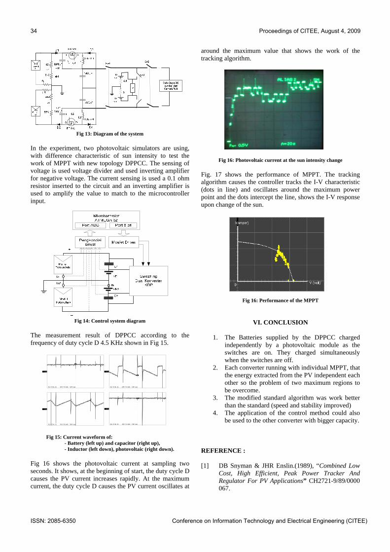
We hope, the result of the proceedings of this conference can be used as reference for the academic and practitioner researchers to gain

At last, I would like to say thank you to all of the committee members, who worked hard to prepare this conference. Special thanks to Electrical Engineering Department, Gadjah Mada University, of supporting on facilities and funds. Thank you and enjoy the conference, CITEE 2009, and the city, Yogyakarta

August, 4Th, 2009

Bambang Sutopo

Electrical Engineering Dept., Fac. of Engineering, GMU

Proceedings of CITEE 2009 Number 1 ISSN: 2085-6350

Table of Contents

Organizer ii Foreword iii Table of Contents v Schedule vii KEYNOTE Social Intelligent on Humanoid Robot: Understanding Indonesian Text Case Study 1 Mauridhi Hery Purnomo (Electrical Engineering Department, ITS, Indonesia) Signal Processing: Video Compression Techniques 4 Dadang Gunawan (Electrical Engineering Department, University of Indonesia) Intelligent Systems Application to Power Systems - Prof. Takashi Hiyama (Kumamoto University, Japan) INTERNATIONAL SESSION: Electrical Power Systems Control System Integrated Starter - DC Motor Couple Three Phase Induction Motor for Automotive Applications 7 Zulkarnain Lubis, Ahmed N. Abdalla, Samsi bin MD said .Mortaza bin Mohamed Transient Stability of SMIB: a Case Study 12 Adelhard Beni Rehiara Look-Up Table of Fuzzy Rule SURAM with AVR ATmega128 17 Zakarias Situmorang Optimal Capacitor Bank Location in the Primary Feeder with Typical Flat Load 25 Hermagasantos Zein Dual Parallel Power Conversion Converter Supplied by Photovoltaic for Base Transceiver Station (BTS) Power Supply 30 Kartono Wijayanto, Yanuarsyah Haroen Integrated ’Buck Converter’ and Wind Turbine Control System Medium Scale (100 W) for Optimization Wind Power and Electricity Power

36

Ali Musyafa, Soedibjo, I Made Yulistiya Negara , Imam Robandi Optimal Power Flow Analysis Using Genetic Algorithm in 500 KV Java Bali Interconnection System 43 Buyung Baskoro, Adi Soeprijanto, Ontoseno Penangsang Transient Stability Assessment of Java Bali 500 KV Multi Machine Electrical Power System Using Committee Neural Network

49

Eko Prasetyo, Boy Sandra, Adi Soeprijanto Overcurrent Protection Coordination Due to Liquid Starter Effect on Large Induction Motor 57 Dimas Anton Asfani, Nalendra Permana Analysis of 20 KV PLN Relay Protection Typical Setting in Industrial Customer 62 Dimas Anton Asfani, Iman Kurniawan, Adi Soeprijanto The Electrical Energy Calculation Based Upon the Voltage Measurement of a High Speed and Magnitude of Multiple Impulse Currents Produced by an Impulse Generator Implemented to ZnO Block

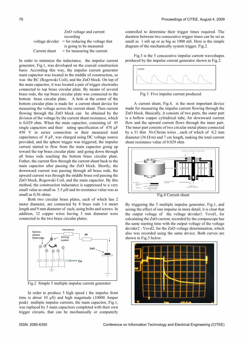
69

Haryono. T, Sirait K.T., Tumiran, Hamzah Berahim Study of Return Voltage Transient in Low Voltage ZnO Arrester Type OBO Bettermann V-20 C/1 73 Nurcahyanto, T. Haryono, Suharyanto The Design of Digital Overcurrent Relay with IEC 60255 Time Curve Characteristic Based on an ATmega16 Microcontroller

77

Agni Sinatria Putra, Tiyono, Astria Nur Irfansyah

Conference on Information Technology and Electrical Engineering (CITEE) v


SCHEDULE Tuesday, August 4, 2009

07.30 – 08.00: Registration 08.00 – 08.15: Opening

1. Welcome speech by conference chairman 2. Speech by GMU’s Rector

08.15 – 09.20: PLENARY SESSION Prof. Takashi Hiyama (Kumamoto University, Japan): Intelligent Systems Application to

Power Systems Prof. Dr. Mauridhi Hery Purnomo (Electrical Engineering Department,ITS, Indonesia):

Social Intelligent on Humanoid Robot: Understanding Indonesian Text Case Study Prof. Dr. Dadang Gunawan (Electrical Engineering Department, University of

Indonesia): Signal Processing: Video Compression Techniques Prof. Dr. Yanuarsyah Haroen (Electrical Engineering and Informatics School, ITB,

Indonesia): Teknologi Sistem Penggerak dalam WahanaTransportasi Elektrik 09.20 – 09.30: Break

PARALLEL SESSION

INTERNATIONAL SESSION (Room 1, 2) Room: 1

Time Group Country/City Author(s) or Presenter(s)

09.30 – 09.45 P Malaysia Zulkarnain Lubis, Ahmed N. Abdalla, Samsi bin MD said .Mortaza bin Mohamed

09.45 – 10.00 P Papua Adelhard Beni Rehiara 10.00 – 10.15 P Medan Zakarias Situmorang 10.15 – 10.30 P Bandung Kartono Wijayanto, Yanuarsyah Haroen 10.30 – 10.45 Coffee Break 10.45 – 11.00 P Bandung Hermagasantos Zein 11.00 – 11.15 P Surabaya Ali Musyafa, Soedibjo, I Made Yulistiya Negara , Imam Robandi 11.15 – 11.30 P Surabaya Buyung Baskoro, Adi Soeprijanto, Ontoseno Penangsang 11.30 – 11.45 P Surabaya Eko Prasetyo, Boy Sandra, Adi Soeprijanto 11.45 – 12.00 P Yogyakarta T. Haryono, Sirait K.T., Tumiran, Hamzah Berahim 12.00 – 13.00 Lunch Break 13.00 – 13.45 P Surabaya Dimas Anton Asfani, Nalendra Permana 13.15 – 13.30 P Surabaya Dimas Anton Asfani, Iman Kurniawan, Adi Soeprijanto

13.30 – 13.45 I Surabaya F.X. Ferdinandus, Gunawan, Tri Kurniawan Wijaya, Novita Angelina Sugianto

13.45 – 14.00 I Surabaya Arya Tandy Hermawan, Gunawan, Tri Kurniawan Wijaya 14.00 – 14.15 I Surabaya Herman Budianto, Gunawan, Tri Kurniawan Wijaya, Eva Paulina Tjendra 14.15 – 14.30 Coffee Break 14.30 – 14.45 I Yogyakarta Bambang Soelistijanto 14.45 – 15.00 I Surakarta Munifah, Lukito Edi Nugroho, Paulus Insap Santosa 15.00 – 15.15 P Yogyakarta Nurcahyanto, T. Haryono, Suharyanto. 15.15 – 15.30 P Yogyakarta Agni Sinatria Putra, Tiyono, Astria Nur Irfansyah

Notes:

1. P: Electrical Power Systems; S: Signals, Systems, and Circuits; I: Information Technology 2. Paper titles are listed in Table of Contents

Department of Electrical Engineering, Faculty of Engineering, Gadjah Mada University


Room: 2 Time Group Country/City Author(s) or Presenter(s)

09.30 – 09.45 S INDIA Ms.M.Thanuja, Mrs. K. SreeGowri 09.45 – 10.00 S Jakarta A. Suhartomo 10.00 – 10.15 S Jakarta Riandini, Mera Kartika Delimayanti, Donny Danudirdjo 10.15 – 10.30 S Jakarta Purnomo Sidi Priambodo, Harry Sudibyo and Gunawan Wibisono 10.30 – 10.45 Coffee Break 10.45 – 11.00 I Yogyakarta Arwin Datumaya Wahyudi Sumari, Adang Suwandi Ahmad 11.00 – 11.15 I Yogyakarta Arwin Datumaya Wahyudi Sumari, Adang Suwandi Ahmad 11.15 – 11.30 I Lampung Sumadi, S; Kurniawan, E. 11.30 – 11.45 S Semarang Florentinus Budi Setiawan 11.45 – 12.00 S Semarang Siswandari N, Adhi Susanto, Zainal Muttaqin 12.00 – 13.00 Lunch Break 13.00 – 13.45 S Yogyakarta Thomas Sri Widodo, Maesadji Tjokronegore, D. Jekke Mamahit 13.15 – 13.30 S Yogyakarta Tarsisius Aris Sunantyo, Muhamad Iradat Achmad 13.30 – 13.45 S Yogyakarta Muhamad Iradat Achmad, Tarsisius Aris Sunantyo, Adhi Susanto 13.45 – 14.00 S Yogyakarta Usman Balugu, Ratnasari Nur Rohmah, Nurokhim 14.00 – 14.15 S Yogyakarta Okky Freeza Prana Ghita Daulay, Arwin Datumaya Wahyudi Sumari 14.15 – 14.30 Coffee Break 14.30 – 14.45 S Yogyakarta Sri Suning Kusumawardani and Bambang Sutopo 14.45 – 15.00 S Yogyakarta Risanuri Hidayat 15.00 – 15.15 S Yogyakarta Budi Setiyanto, Astria Nur Irfansyah, and Risanuri Hidayat 15.15 – 15.30 S Yogyakarta Budi Setiyanto, Mulyana, and Risanuri Hidayat

NATIONAL SESSION (Room 3, 4, 5, 6, 7)

Yogyakarta, August 4, 2009

Proceedings of CITEE, August 4, 2009 Keynote - 1

Social Intelligent on Humanoid Robot: Understanding Indonesian Text

Case Study

Mauridhi Hery Purnomo Electrical Engineering Department-Institut Teknologi Sepuluh November

Surabaya 60111, Indonesia [email protected]

Abstract— Social affective and emotion are required on

humanoid robot performance to make the robot be more human. Social intelligent are the individual ability to manage relationship with other agents and act wisely based on previous learning experiences. Here, social intelligent is intended to understand Indonesian text. How the computation process, as well as affective interaction, emotion expression of the humanoid robot to the human statement. This process is a highly adaptive complex approximation, dependently on its entire situation and environment.

Keywords—social, affective, emotion, intelligent, computing (key words)

I. INTRODUCTION Social and interactive behaviors are necessary

requirements in wide implementation areas and contexts where robots need to interact and collaborate with other robots or humans. The nature of interactivity and social behavior in robot and humans is a complex model.

An experimental robot platform KOBIE, which provides a simulation tool for emotion expression system includes an emotion engine was developed. The simulation tool provides a visualization interface for the emotion engine and expresses emotion through an avatar. The system can be used in the development of cyber characters that use emotions or in the development of an apparatus with emotion in a ubiquitous environment [1]. To improve the understandability and friendliness in human-computer interfaces and media contents, a Multimodal Presentation Markup Language (MPML) is developed. MPML is a simple script language to make multi-modal presentation contents using animated characters for presenters [2]. Other effort in the robot head which uses arm-type antennae, eye-expression, and additional exaggerating parts for dynamic emotional expression is also developed. The robot head is developed for various and efficient emotional expressions in the Human-Robot interaction field. The concept design of the robot is an insect character [3]. In regard to artificial cognitive, iCub humanoid robot systems is developed. The system is open-systems 53 degree-of-freedom cognitive humanoid robot, 94 cm tall, the same size as a three year-old child. Able to crawl on all fours and sit up, its hands will allow dexterous manipulation, and its head and eyes are fully articulated. It

has visual, vestibular, auditory, and haptic sensory capabilities [4]. An innovative integration of interactive group learning, multimedia technology, and creativity used to enhance the learning of basic psychological principles was created. This system is based on current robotic ideology calling for the creation of a PowerPoint robot of the humanoid type that embodies the basic theories and concepts contained in a standard psychological description of a human being [5]. Now days, not only visual and auditory information are used in media and interface fields but also multi-modal contents including documents such like texts. Thus, in this paper, a part of result on emotion expression and environment through understanding Indonesian text, as affective interaction between a human and a robot is explored. The paper is organized as follows. In Section 2, the general emotion and expression system on life-like agent is presented. Section 3 describes the experimental on Indonesian text classification. In Section 4, the preliminary result in emotion classification of Indonesian article text is discussed.

II. EMOTION AND EXPRESSION ON LIFE-LIKE AGENT

Social Computing, Social Agent, and Life-likeness Many Psychologists have studied a definition and classification of emotions, therefore, so many classification methods of emotions and expressions. However, we need to choose categories of emotions that are suitable expressed by robot, as well as the well-known Ekman’s 6 basic emotion expressions model can be used.

In social computing life-like characters are the key, and the affective functions create believability. To articulate synthetic emotions can be presented as; personalities, human interactive behavior or presentation skills. The personalities; by means of body movement, facial display, and the coordination of the embodied conversational behavior of multiple characters possibly including the user. Personality is key to achieving life-likeness

Some Applications of Life-Like Character

Life-like characters are synthetic agents apparently living on the screen of computers. Life-like character can be implemented as virtual tutors and trainers in interactive learning environments. On the web as an information expert, presenter, communication partners, and enhancing the search engine. The other application as actors for entertainment, in

Conference on Information Technology and Electrical Engineering (CITEE) ISSN: 2085-6350

2 Keynote Proceedings of CITEE, August 4, 2009

online communities and guidance systems as personal representatives.

Early characterization of the emotional and believable character was raised by Joseph Bates. He said, the portrayal of emotions plays a key role in the aim to create believable characters, one that provides the illusion of life, and thus permits the audience’s suspension of disbelief. In game and animation, suspension of disbelief is very important, for instance as: synthetic actors, non-player characters, and embodied conversational agents.

Emotion and personality are often seen as the affective bases of believability, and sometimes the broader term social is used to characterize life-likeness.

III. CLASSIFICATION SYSTEM FOR INDONESIAN TEXT Information growth, including texts are faster than

human ability, thus help system is quite necessary. For instance as the following illustration;

The Recent study, which used Web searches in 75 different languages to sample the Web, determined that there were over 11.5 billion (1012) Web pages in the publicly indexable Web as of the end of January 2005

As of March 2009, the indexable web contains at least 25.21 billion pages

On July 25, 2008, Google software engineers Jesse Alpert and Nissan Hajaj announced that Google Search had discovered one trillion unique URLs

As of May 2009, over 109.5 million websites operated

label

traininginput

languagedependentNLP tools

featureextractor ..features..

machinelearning

classifiermodel

testinput

languagedependentNLP tools

featureextractor ..features.. predicted

label

(b) prediction phase

(a) training phase

Figure 1. Example of Indonesian Text Classification

FreeText

KnowledgeBase

InformationRetrieval

Text-basedConversational Agent

User (Human)

TextInput

Response

TextClassification

TextMining

Figure 2. Knowledge from Free (Unstructured) Text

The illustrations as mentioned above explain the essential of help system especially in Indonesian text. We have developed a system for understanding and classifying Indonesian text, and the block diagram as shown in figure 1 and figure 2.

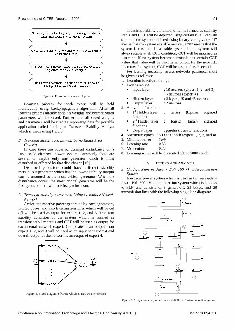
Figure 1 is an example how to train machine (agent) in order responsive to the external and adequate response. The case study is, Indonesian text classification. There are two types of machine learning, supervised and unsupervised learning.

Figure 2 show a block diagram process of embodied conversational agent.

IV. EMOTION CLASSIFICATION FROM INDONESIAN ARTICLE TEXT

The following sentences are sample of statements, and some emotion expressions;

• “When a car is overtaking another and I am forced to drive off the road” → anger

• “When I nearly walked on a blindworm and then saw it crawl away” → disgust

• “When I was involved in a traffic accident” → fear

• “I do not help out enough at home” → guilt

• “Passing an exam I did not expect to pass” → joy

• “Failing an examination” → sadness

• “When, as an adult I have been caught lying or behaving badly” → shame

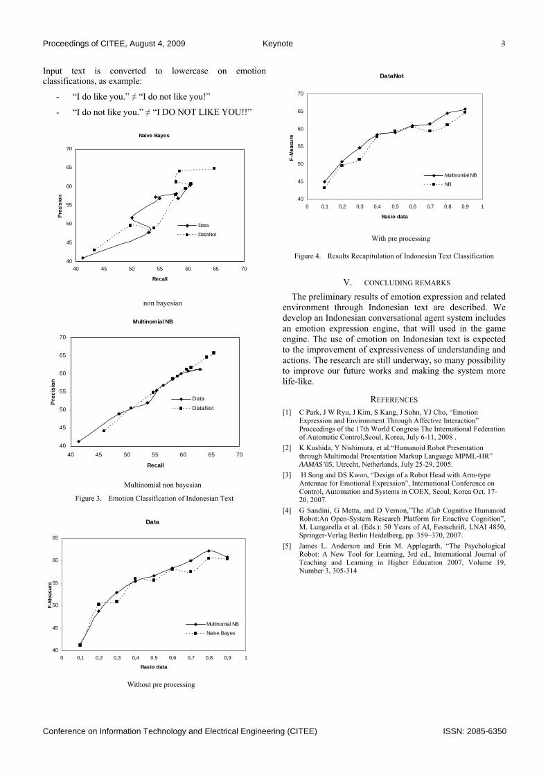
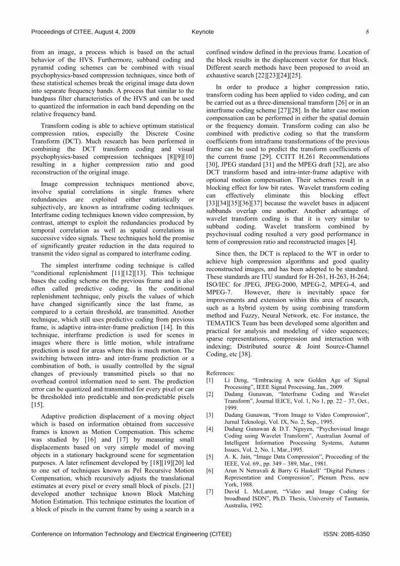
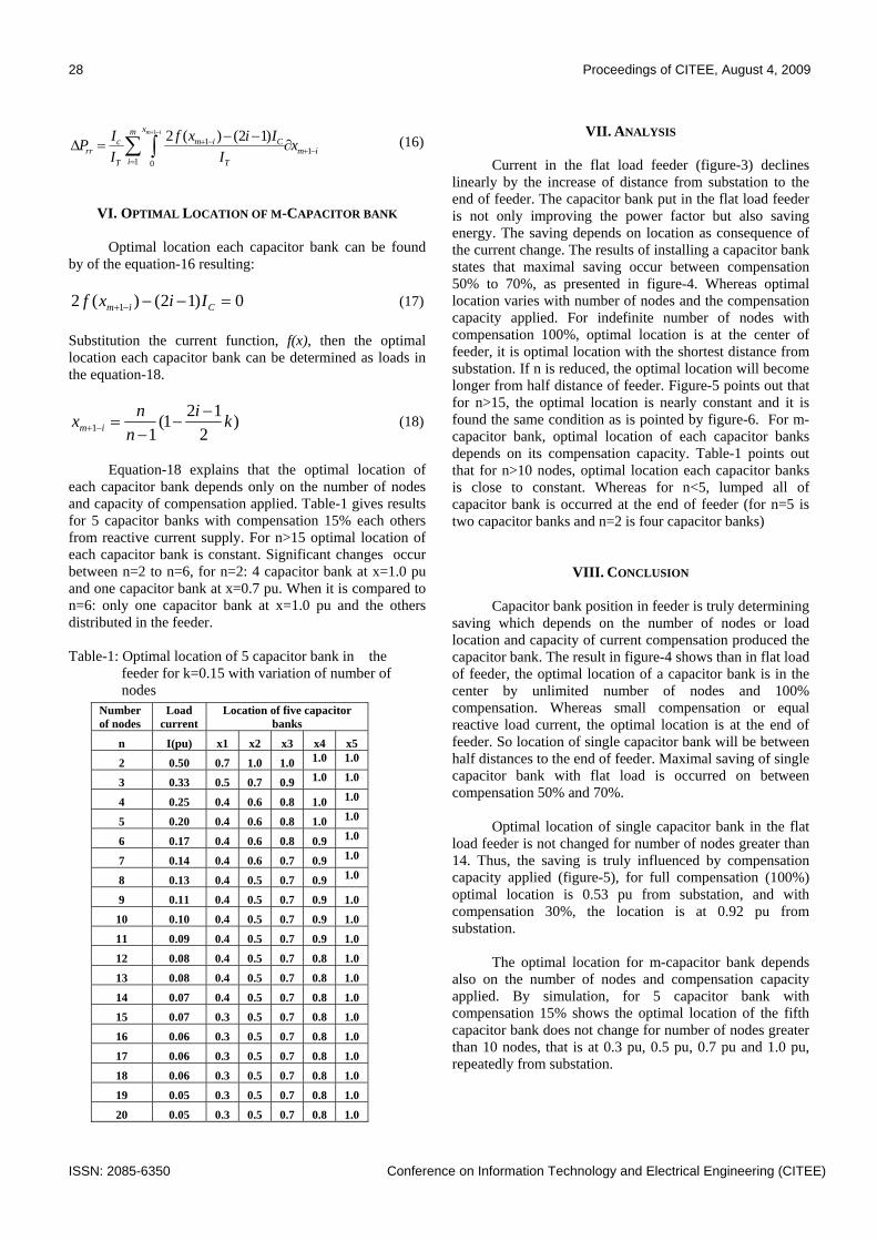
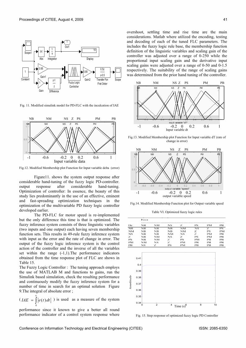
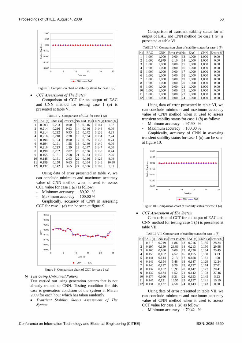
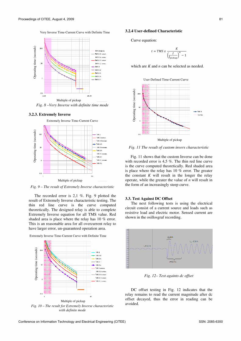
Based on some statements and the emotion expression as mentioned above in Indonesian text, the preliminary classification results are shown in the table 1, figure 3 and figure 4.

The classification is divided into six (6) classes of emotion: disgust, shame, anger, sadness, joy and fear. Each class has 200 text files, data: “as-is”; DataNot: pre-processing only handles “not”. Split ratio 0.5 shows f-measure scores 0.59

Pre-processing Steps

Text Classification (TC) techniques usually ignore stop-words and case of input text. In pre-processing step, stop-words removal can be applied.

Stop-words such as “not”, “in”, “which” and exclamation marks (“!”) usually do not affect categorization of text.

TABLE I. NAÏVE BAYES CLASSIFICATION INTO 4 CLASS

Accuracy (%) Classification ratio

(%) Usual & original text Text without stop words

20 71.41 69.81

40 73.33 71.3

60 74.40 71.3

80 75.33 74.05

Example:

- Microsoft released Windows → categorized as “news”.

- Microsoft has not released Windows yet → still categorized as “news”.

ISSN: 2085-6350 Conference on Information Technology and Electrical Engineering (CITEE)


Input text is converted to lowercase on emotion classifications, as example:

- “I do like you.” ≠ “I do not like you!”

- “I do not like you.” ≠ “I DO NOT LIKE YOU!!”

Naive Bayes

40

45

50

55

60

65

70

40 45 50 55 60 65 70

Recall

Prec

isio

n

Data

DataNot

non bayesian

Multinomial NB

40

45

50

55

60

65

70

40 45 50 55 60 65 70

Recall

Prec

isio

n

Data

DataNot

Multinomial non bayesian

Figure 3. Emotion Classification of Indonesian Text

Data

40

45

50

55

60

65

0 0,1 0,2 0,3 0,4 0,5 0,6 0,7 0,8 0,9 1

Rasio data

F-M

easu

re

Multinomial NB

Naive Bayes

Without pre processing

DataNot

40

45

50

55

60

65

70

0 0,1 0,2 0,3 0,4 0,5 0,6 0,7 0,8 0,9 1

Rasio data

F-M

easu

re

Multinomial NB

NB

With pre processing

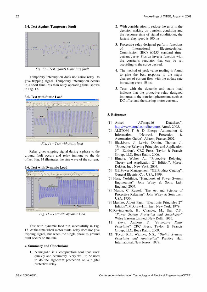
Figure 4. Results Recapitulation of Indonesian Text Classification

V. CONCLUDING REMARKS The preliminary results of emotion expression and related environment through Indonesian text are described. We develop an Indonesian conversational agent system includes an emotion expression engine, that will used in the game engine. The use of emotion on Indonesian text is expected to the improvement of expressiveness of understanding and actions. The research are still underway, so many possibility to improve our future works and making the system more life-like.

REFERENCES [1] C Park, J W Ryu, J Kim, S Kang, J Sohn, YJ Cho, “Emotion

Expression and Environment Through Affective Interaction” Proceedings of the 17th World Congress The International Federation of Automatic Control,Seoul, Korea, July 6-11, 2008 .

[2] K Kushida, Y Nishimura, et al.“Humanoid Robot Presentation through Multimodal Presentation Markup Language MPML-HR” AAMAS’05, Utrecht, Netherlands, July 25-29, 2005.

[3] H Song and DS Kwon, “Design of a Robot Head with Arm-type Antennae for Emotional Expression”, International Conference on Control, Automation and Systems in COEX, Seoul, Korea Oct. 17-20, 2007.

[4] G Sandini, G Metta, and D Vernon,”The iCub Cognitive Humanoid Robot:An Open-System Research Platform for Enactive Cognition”, M. Lungarella et al. (Eds.): 50 Years of AI, Festschrift, LNAI 4850, Springer-Verlag Berlin Heidelberg, pp. 359–370, 2007.

[5] James L. Anderson and Erin M. Applegarth, “The Psychological Robot: A New Tool for Learning, 3rd ed., International Journal of Teaching and Learning in Higher Education 2007, Volume 19, Number 3, 305-314



Signal Processing: Video Compression Techniques

Dadang Gunawan

Electrical Engineering Department, University of Indonesia

In our information society, signal processing has been created a significant effect. Signal processing can be found everywhere: in home appliances, in Cell Phone, TVs, Automobile, GPSs, Modem Scanner, and All kind of Communication Systems and Electronic Devices. Modern cell phones are indeed a most typical example – within these small wonders, voice, audio, image, video and graphics are processed and enhanced based on decades of media signal processing research.

Technological advancement in recent years has proclaimed a new golden age for signal processing [1]. Many exciting directions, such as bioinformatics, human language, networking, and security, are emerging from traditional field of signal processing on raw information content. The challenge in the new era is to transcend from the conventional role of processing in low level, waveform-like signal to the new role of understanding and mining the high-level, human-centric semantic signal and information. Such a fundamental shift has already taken place in limited areas of signal processing and is expected to become more pervasive in coming years of research in more areas of signal processing.

One of the huge applications of signal processing is exploited as video compression. Nowadays, video applications such as digital laser disc, electronic camera, videophone and video conferencing systems, image and interactive video tools on personal computers and workstations, program delivery using cable and satellite, and high-definition television (HDTV) are available for visual communications. Many of these applications, however, require the use of data compression because visual signals require a large communication bandwidth for transmission and a large amounts of computer memory for storage [2][3]. In order to make the handling of visual signals cost effective it is important that their bandwidth be compressed as much as possible. Fortunately, visual signals contain a large a mount of statistically and psychovisually redundant information [4]. By removing this unnecessary information, the amount of data necessary to adequately represent an image can be reduced.

The removal of unnecessary information generally can be achieved by using either statistical compression techniques or psychovisual compression techniques. Both techniques result in a loss information, but in the former the loss may be recovered by signal processing such as filtering and inter or intra-polation. In the later, information is in fact discarded, but in way that is not perceptible to a human observer. The later techniques offer much greater levels of

compression but it is no longer possible to perfectly reconstructed the original image [4]. While the aim in psychovisual coding is to keep these differences at an imperceptible level, psychovisual compression inevitably involves a tradeoff between the quality of the reconstructed image and the compression rate achieved. This tradeoff can often be assessed using mathematical criteria, although a better assessment is in general provided by human observer.

The applications of image data compression, in general, are primarily in the transmission and storage of information. In transmission, applications such as broadcast television, teleconferencing, videophone, computer-communication, remote sensing via satellite or aircraft, etc., require the compression techniques to be constrained by the need

For the real time compression and on-line consideration which tends to severely limit the size and hardware complexity. In storage applications such as medical images, educational and business documents, etc., the requirements are less stringent because much of the compression processing can be done off-line. However, he decompression or retrieval should still be quick and efficient to minimize the response time [5].

All images of interest usually contain a considerable amount of statistically and subjectively superfluous information [6]. A statistical image compression technique exploits statistical redundancies in the information in the image. This technique reduces the amount of data to be transmitted or to be stored in an image without any information being lost. The alternative is to discard the subjective redundancies in an image, which leads to psychovisual image compression. These psychovisual techniques rely on properties of the Human Visual characteristic system (HVS) to be determined which features will not be noticed by human observer.

There are numerous way to achieve compression in statistical image compression techniques such as Pulse Code Modulation (PCM), Differential PCM (DPCM), Predictive Coding, Transform Coding, Pyramid Coding and Subband Coding, as well as Psychovisual Coding techniques. Statistical compression techniques all use a form of amplitude quantization in their algorithms to improve compression performance. Simple quantization alone, however, is not the most efficient or flexible techniques to combine with a statistical compression algorithm [7]. The combination of quantization and psychophysics, on the other hand has the potential to remove most subjectively redundant information efficiently



from an image, a process which is based on the actual behavior of the HVS. Furthermore, subband coding and pyramid coding schemes can be combined with visual psychophysics-based compression techniques, since both of these statistical schemes break the original image data down into separate frequency bands. A process that similar to the bandpass filter characteristics of the HVS and can be used to quantized the information in each band depending on the relative frequency band.

Transform coding is able to achieve optimum statistical compression ratios, especially the Discrete Cosine Transform (DCT). Much research has been performed in combining the DCT transform coding and visual psychophysics-based compression techniques [8][9][10] resulting in a higher compression ratio and good reconstruction of the original image.

Image compression techniques mentioned above, involve spatial correlations in single frames where redundancies are exploited either statistically or subjectively, are known as intraframe coding techniques. Interframe coding techniques known video compression, by contrast, attempt to exploit the redundancies produced by temporal correlation as well as spatial correlations in successive video signals. These techniques hold the promise of significantly greater reduction in the data required to transmit the video signal as compared to interframe coding.

The simplest interframe coding technique is called “conditional replenishment [11][12][13]. This technique bases the coding scheme on the previous frame and is also often called predictive coding. In the conditional replenishment technique, only pixels the values of which have changed significantly since the last frame, as compared to a certain threshold, are transmitted. Another technique, which still uses predictive coding from previous frame, is adaptive intra-inter-frame prediction [14]. In this technique, interframe prediction is used for scenes in images where there is little motion, while intraframe prediction is used for areas where this is much motion. The switching between intra- and inter-frame prediction or a combination of both, is usually controlled by the signal changes of previously transmitted pixels so that no overhead control information need to sent. The prediction error can be quantized and transmitted for every pixel or can be thresholded into predictable and non-predictable pixels [15].

Adaptive prediction displacement of a moving object which is based on information obtained from successive frames is known as Motion Compensation. This scheme was studied by [16] and [17] by measuring small displacements based on very simple model of moving objects in a stationary background scene for segmentation purposes. A later refinement developed by [18][19][20] led to one set of techniques known as Pel Recursive Motion Compensation, which recursively adjusts the translational estimates at every pixel or every small block of pixels. [21] developed another technique known Block Matching Motion Estimation. This technique estimates the location of a block of pixels in the current frame by using a search in a

confined window defined in the previous frame. Location of the block results in the displacement vector for that block. Different search methods have been proposed to avoid an exhaustive search [22][23][24][25].

In order to produce a higher compression ratio, transform coding has been applied to video coding, and can be carried out as a three-dimensional transform [26] or in an interframe coding scheme [27][28]. In the latter case motion compensation can be performed in either the spatial domain or the frequency domain. Transform coding can also be combined with predictive coding so that the transform coefficients from intraframe transformations of the previous frame can be used to predict the transform coefficients of the current frame [29]. CCITT H.261 Recommendations [30], JPEG standard [31] and the MPEG draft [32], are also DCT transform based and intra-inter-frame adaptive with optional motion compensation. Their schemes result in a blocking effect for low bit rates. Wavelet transform coding can effectively eliminate this blocking effect [33][34][35][36][37] because the wavelet bases in adjacent subbands overlap one another. Another advantage of wavelet transform coding is that it is very similar to subband coding. Wavelet transform combined by psychovisual coding resulted a very good performance in term of compression ratio and reconstructed images [4].

Since then, the DCT is replaced to the WT in order to achieve high compression algorithms and good quality reconstructed images, and has been adopted to be standard. These standards are ITU standard for H-261, H-263, H-264; ISO/IEC for JPEG, JPEG-2000, MPEG-2, MPEG-4, and MPEG-7. However, there is inevitably space for improvements and extension within this area of research, such as a hybrid system by using combining transform method and Fuzzy, Neural Network, etc. For instance, the TEMATICS Team has been developed some algorithm and practical for analysis and modeling of video sequences; sparse representations, compression and interaction with indexing; Distributed source & Joint Source-Channel Coding, etc [38].

References: [1] Li Deng, “Embracing A new Golden Age of Signal

Processing”, IEEE Signal Processing, Jan., 2009. [2] Dadang Gunawan, “Interframe Coding and Wavelet

Transform”, Journal IEICE, Vol. 1, No 1, pp. 22 – 37, Oct., 1999.

[3] Dadang Gunawan, “From Image to Video Compression”, Jurnal Teknologi, Vol. IX, No. 2, Sep., 1995.

[4] Dadang Gunawan & D.T. Nguyen, “Psychovisual Image Coding using Wavelet Transform”, Australian Journal of Intelligent Information Processing Systems, Autumn Issues, Vol. 2, No. 1, Mar.,1995.

[5] A. K. Jain, “Image Data Compression”, Proceeding of the IEEE, Vol. 69., pp. 349 – 389, Mar., 1981.

[6] Arun N Netravali & Barry G Haskell’ “Digital Pictures : Representation and Compression”, Plenum Press, new York, 1988.

[7] David L McLarent, “Video and Image Coding for broadband ISDN”, Ph.D. Thesis, University of Tasmania, Australia, 1992.



[8] K. N. Ngan, K. S. Leong & H. Singh, “Adaptive Cosine Transform Coding of Images in perceptual Domain”, IEEE Transaction ASSP, Vo. 37, pp. 1743 – 1750, Nov., 1989.

[9] B Chitprasert & K. R. Rao, “Human Visual Weighted progressive Image Transmission”, IEEE Transaction on Communication, Vol. 38, pp. 1040 – 1044, Jul. 1990.

[10] D. L. McLaren & D. T. Nguyen, “The Removal Subjective redundancy fro DCT Coded Images”, IEE Proceeding – Part I, Vol. 138, pp. 345 – 350, Oct. 1991.

[11] F. W. Mounts, “A Video Coding System with Conditional Picture-Element Replenishment”, The Bell System Technical Journal, Vol. 48, pp. 2545 – 2554, Sep. 1969.

[12] J. C. Candy, “Transmitting television as Clusters of Frame to frame Differences”, The Bell System Technical Journal, Vol. 50, pp. 1889 – 1917, Aug. 1971.

[13] [B. G. Haskel, F. W. Mount and C. Candy, “Interframe Coding of Videotelephone Pictures”, Proceeding of IEEE, Vol. 60, pp. 792 – 800, Jul. 1972.

[14] D. Westerkamp, “Adaptive Intra-Inter frame DPCM-Coding for Transmission TV-Signals with 34 Mbps”, IEEE Zurich Seminar on digital Communication, pp. 39 – 45, Mar. 1984.

[15] M. H. Chan, “Image coding Algorithms for Video-conferencing Applications”, Ph.D. Thesis Imperial College – University of London, 1989.

[16] J. O. Limb & J. A. Murphy, “Measuring the Speed of Moving Objects from television Signals”, IEEE Transaction on Communication, Vol. 23, pp. 474 – 478, Apr. 1975.

[17] C. Cafforio & F Rocca, “Methods of Measuring Small Displacements of Television Images”, IEEE Transaction on Information Theory, Vol. 22, pp.573 – 579, Sep. 1976.

[18] A. N. Netravali & J. D. Robbins, “Motion Compensated television Coding ; Part 1”, The Bell-System Technical Journal, Vol. 58, pp. 631 – 670, Mar. 1979.

[19] C. Cafforio & F Rocca, “The Differential method for Motion Estimation”, Image Science Processing & Dynamic Scene Analysis, Springer Verlag, New York, pp. 104 – 124, 1983.

[20] J. D. Robbins & A. N. Netravali, “Recursive motion compensation : A Review”, mage Science Processing & Dynamic Scene Analysis, Springer Verlag, New York, pp. 75, 1983.

[21] J. R. Jain & A. K. Jain, “Displacement measurement & Its Application in Interframe Image Coding”, IEEE Transaction on Communication, Vol. 29, pp. 1799 – 1808, Dec. 1981.

[22] T. Koga, K.Iinuma, A. Hirano, Y. Iijima & T. Ishiguro, “Motion-compensated Interframe Coding for Video Conferencing”, Proceeding National Telecommunication Conference, New Orleans, LA., pp. G5.3.1 – 5.3.5, Nov. 1981.

[23] R. Srinivasan & K. R. Rao, “Predictive Coding Based on Efficient Motion Compensation”, IEEE International Conference on Communication, Amsterdam, pp. 521 – 526, May 1984.

[24] A. Puri, H. M. Hang & D. L. Schilling, “An Efficient Block matching Algorithm for Motion Compensated Coding”, Proceeding IEEE ICASSP, pp. 25.4.1 – 25.4.4, 1987.

[25] M. Ghanbari, “The Cross Search Algorithm for Motion Compensation”, IEEE Transaction on Communication, Vol. 38, pp. 950 – 953, Jul. 1990.

[26] M. Gotze & G Ocylock, “An Adaptive Interframe Transform Coding System for Images”, proceeding IEEE ICASSP 82, pp. 448 – 451, 1982.

[27] J. R. Jain & A. K. Jain, “Displacement measurement & Its Application in Interframe Image Coding”, IEEE Transaction on Communication, Vol. 29, pp. 1799 – 1808, Dec. 1981.

[28] J. A. Roese, W. K. Pratt & G. S. Robinson, “Interframe Cosine Transform Image Coding, “ IEEE Transaction on Communication, Vol. 25, pp. 1329 – 1338, Nov. 1977.

[29] J. A. Roese, “Hybrid Transform predictive Image Coding in Image Transmission Techniques, Academic Press, new York, 1979.

[30] CCITT H.261 Recommendations, “Video Codec for Audiovisual Services at p x 64 kbps”, 1989.

[31] G. Wallace, “The JPEG Stil Picture Compression Standard”, Communication ACM, Vol. 34, pp. 30 – 44, Apr. 1991.

[32] D. LeGall, “MPEG : A Video Compression Standard for Multimedia Applications”, Communication ACM, Vol. 34, pp. 46 – 58, Apr. 1991.

[33] S. G. Mallat, “A Theory for Multiresolution Signal Decomposition : the Wavelet Representation” IEEE Transaction on Pattern Analysis & Machine Intelligent, Vol. 11, pp. 674 – 693, Jul. 1989.

[34] S. G. Mallat, “Multifrequency Channel Decomposition of Image and Wavelet Models”, IEEE Transaction on ASSP, Vol. 37, pp. 2091 – 2110, Dec. 1989.

[35] O Riol & M. Vetterli, “Wavelet & Signal Processing”, IEEE Signal Processing Magazine, Vol. 8, pp. 14 – 38, Oct. 1991.

[36] Y. Q. Zhang & S. Zafar, “Motion-Compensated Wavelet Transform Coding for Color Video Compression”, IEEE Transaction on Circuit & Systems for Video Technology, Vol. 2, pp. 285 – 296, Sep. 1992.

[37] S. Zafar, Y. Q. Zhang & B. Jabbari, “Multiscale Video Representation Using Multiresolution Compensation & Wavelet Decompostion“, IEEE Journal Selected Area in Communications, Vol. 11, pp. 24 – 34, Jan. 1993.

[38] Project Team Tematics, “Activity Report”, INRIA, 2008.


Proceedings of CITEE, August 4, 2009 7


CONTROL SYSTEM INTEGRATED STARTER - DC MOTOR COUPLE THREE PHASE INDUCTION MOTOR FOR AUTOMOTIVE APPLICATIONS

Zulkarnain Lubis, Ahmed N. Abdalla Faculty of Electrical and electronic Eng., University Malaysia Pahang, Kuantan 26300, Malaysia

[email protected] [email protected]

Samsi bin MD said .Mortaza bin Mohamed

Faculty of Electrical and electronic Eng., TATI University College ,Kemaman 24000 Terengganu Malaysia. Mortaza @ump.edu.my [email protected]

Abstract-An electric vehicle control system controls motor response based upon monitored vehicle characteristics to provide consistent vehicle performance under a variety of conditions for a given accelerator manipulation. With emphasis on a cleaner environment and efficient operation, vehicles today rely more and more heavily on electrical power generation for success. With the oil price shocks of the past few decades, as well as an increasing awareness of the emissions of air pollutants and greenhouse gases from cars and trucks, the interest to investigate alternative vehicle propulsion systems has grown. This challenge of fuel economy standards is promoting optimised and sometimes novel vehicle power automotive architectures, which combine the traditional internal combustion engine (ICE) with various forms of electric drives. The different types of the hybrid electric vehicles (HEV) are real competitors of the classical ICE driven cars. The controller of induction motor (IM) is designed based on input-output feedback linearization technique. It allows greater electrical generation capacity and the fuel economy and emissions benefits of hybrid electric automotive propulsion. Finally, a typical series hybrid electric vehicle is modelled and investigated. Control system integrated starter dc motor couple three phase induction motor for automotive applications. Various tests, such as acceleration traversing ramp, and fuel consumption and emission are performed on the proposed model of 3 phase induction motor coupler dc motor in electric hybrid vehicles drive. Keywords: hybrid electrical vehicle, Induction motor, Dc Machine.

I. INTRODUCTION With the oil price shocks of the past few decades, as well as an increasing awareness of the emissions of air pollutants and greenhouse gases from cars and trucks, the interest to investigate alternative vehicle propulsion systems has grown. This challenge of fuel economy standards is promoting optimised and sometimes novel vehicle powertrain architectures, which combine the traditional internal combustion engine (ICE) with various forms of electric drives. The different types of the hybrid electric vehicles (HEV) are real competitors of the classical ICE driven cars.

In an all-electric vehicle (EV) there is no ICE, but all other components exist including batteries with excessive power. EVs and HEVs are studied by numerous authors in the past, one comprehensive study is that of Chan [1]. First full-scale hybrid vehicle work in Turkey is Doblo/Tofas example realized at Marmara Research Center [2]. There have been university theses and an industry project constitutes the basics of this paper [3-7]. One of the main contribution is that of Gokce [4], energy conservation and energy balance method is adopted. The input-output feedback linearization technique combined with an adaptive backstopping observer in stator reference frame the induction motor [5] using in series hybrid electric vehicle is controlled. This paper focus on a new HEV modelling to make a couple two electric motor IM and DCM close loop sinusoidal PWM inverter to control the speed of a three phase induction motor. This compact inverter had its hardware reduced to a minimum through the use of a programmable integrated circuit (PIC) micro-controller (PIC16C73A). In this sense a microcomputer interface was avoided. At the end, a typical HEV is modelled and investigated. Simulation results obtained show the IM and other components performances for a typical city drive cycle. 2. Theoretical background 2.1 Management control system HEV A hybrid electrical vehicle may consist of an internal combustion engine (ICE), electric motor (EM), electric generator (EG), power electronic circuits, advanced electronic control units (ECU), a complex mechanical transmission and a battery bank.

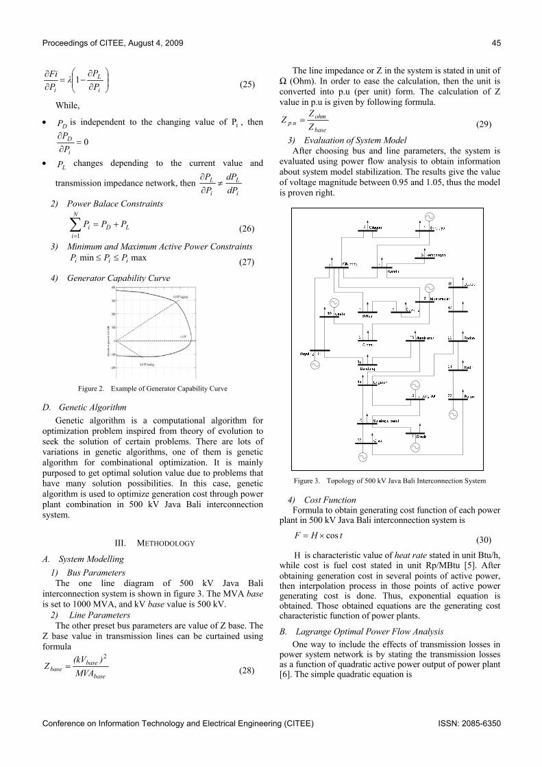
Fig.1 shows the structure of drive assembly of a hybrid electric car. There are 3 electrical machines, generator and starter (M/G), starter and the main motor (M), in the figure. G/M is an integrated started and generator (ISG) which connects with the internal combustion engine (ICE) using a couple . The starter is a standby one. The M, which is subject of this paper, is called main motor. It connects with the wheels through the final gear. Main motor is a three phase asynchronous Motor. The battery pack is a 288V, 10Ah NiH one. Fig.1

8 Proceedings of CITEE, August 4, 2009


Fig.1 Management control system HEV The hybrid electric car has 8 working modes: idle stop, ICE drive motor drive, serial mode, parallel mode, serial & parallel mode, ICE drive, battery charge and regenerative braking. Fig.1 shows four of the modes. ICE stops running when it is in the idle running state, and may be restarted in less than 100ms by the M/G. The idle stop mode will reduce fuel consumption and emissions in idle running state. The ICE drive mode is the same as the traditional car and will occur in most efficient working area of ICE. The motor drive mode is the same as the battery electric car and will occur at very low speed. In variasi mode which is shown in Fig.1, the ICE drags the M/G to charge the battery, and the main induction motor. The first step in vehicle performance modelling is to write an equation for the electric force . This is the force transmitted to the ground through the drive wheels, and propelling the vehicle forward. This force must overcome the road load and accelerate the vehicle as shown in Fig.2

Fig.2 Basic of forces on a vehicle

The rolling resistance is primarily due to the friction of the vehicle tires on the road and can be written as:

froll = fr Mg , (1)

where M is the vehicle mass, f , is the rolling resistance coefficient and g is gravity acceleration .

The aerodynamic drag is due to the friction of the body of vehicle moving through the air. The formula for this component is as in the following .Dynamic modelling and simulation of an induction motor with

fAD = ξCD AV2 (2)

The gravity force due to the slope of the road can be expressed by:

fgrade = Mg. sin α (3)

Where α is the grade angle.

In addition to the forces shown in Fig.3, another one is needed to provide the linear acceleration of the vehicle given by:

facc =Mα = M (4)

The propulsion system must now overcome the road loads and accelerate the vehicle by the tractive force, Ftot , as follows :

Ftot = froll + fAD + fgarde + facc (5)

Whells and axels convert Ftot and the speed of vehicle to torque and angular speed requirements for differential as follow :

Twhell = Ftot rwheel , ωwheel = V/ rwheel (6)

Where Twhell , rwheel and ωwheel are the tractive torque, the radius, and the angular velocity at the wheels, respectively.

The angular torque velocity and torque of the wheels are converted to motor rpm and motor torque requirements using the gears ratio at differential and gearbox as follows :

ω m = Gfd Ggb ωwheel , Tm = Twhell / Gfd Ggb (7)

Where Gfd and Ggb are respectively differential and gear box gears ratios.

3.PROPOSED METHOD

3.1.Controllers couple IM and DCM

The coupling of these two components can be in parallel or in series. In the parallel configuration, both the IM and the DC electric motor contribute to the traction force that moves the vehicle. Power is split between them according to a control strategy, which is usually implemented by a



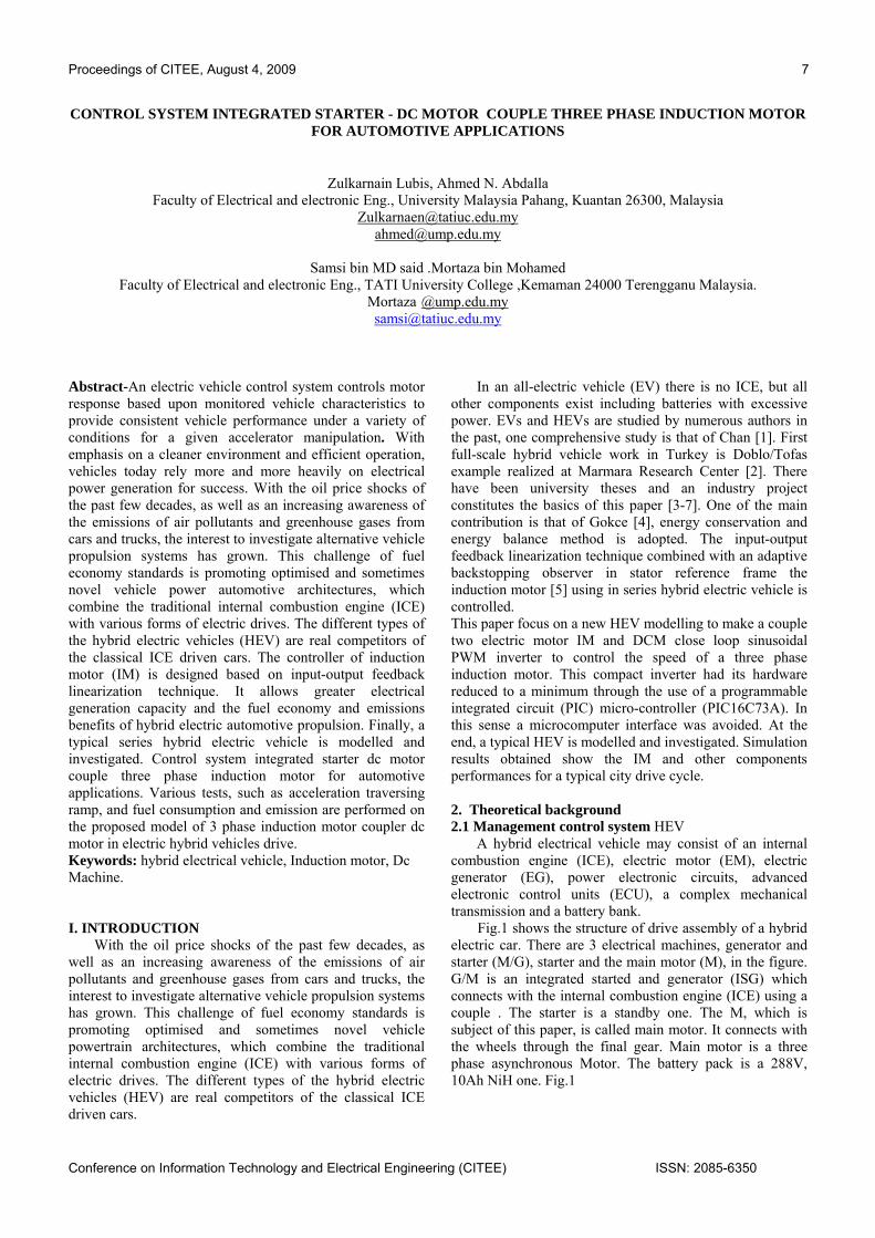
supervisory controller. Two different sub-controllers independently control the IM and the DC motor. Both sub-controllers receive their commands from the supervisory controller. Among these commands are the two torque requests required from both sub-systems as shown in Fig.3.

Fig.3 Controllers IM and DCM in a typical HEV application

4. CONTROLLER SIMULATION MODEL

To study the performance of the developed Transient torque and current model, a closed loop torque control of the drive is simulated using Matlab/Simulink simulation package. Fig.4 shows the simulation block diagram[9]. The drive cycle gives the required vehicle speed then the torque and speed requested from the electric motor. The current drawn from IM power supply shows the battery performance. The dynamic behaviour of the IM in the DCM+IM drive cycle. Power assembly diagram of HEV Normal Condition the ECE drive cycle. IM torque and average torque, power assembly diagram of HEV in Hybrid Electric. The block diagram of the simulink model is shown in Fig.4.

Fig.4. Simulation block diagram for stability control

Fig.5. Developed model of transient torque and current control of induction machine

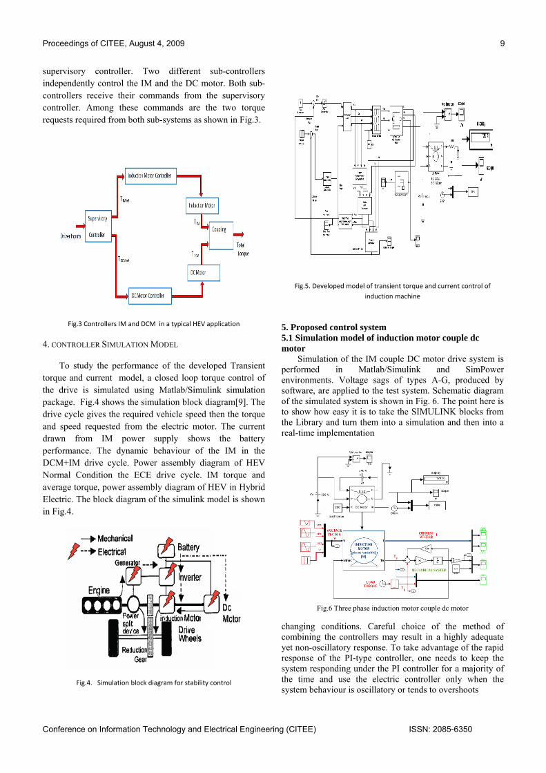
5. Proposed control system 5.1 Simulation model of induction motor couple dc motor Simulation of the IM couple DC motor drive system is performed in Matlab/Simulink and SimPower environments. Voltage sags of types A-G, produced by software, are applied to the test system. Schematic diagram of the simulated system is shown in Fig. 6. The point here is to show how easy it is to take the SIMULINK blocks from the Library and turn them into a simulation and then into a real-time implementation

Fig.6 Three phase induction motor couple dc motor

changing conditions. Careful choice of the method of combining the controllers may result in a highly adequate yet non-oscillatory response. To take advantage of the rapid response of the PI-type controller, one needs to keep the system responding under the PI controller for a majority of the time and use the electric controller only when the system behaviour is oscillatory or tends to overshoots



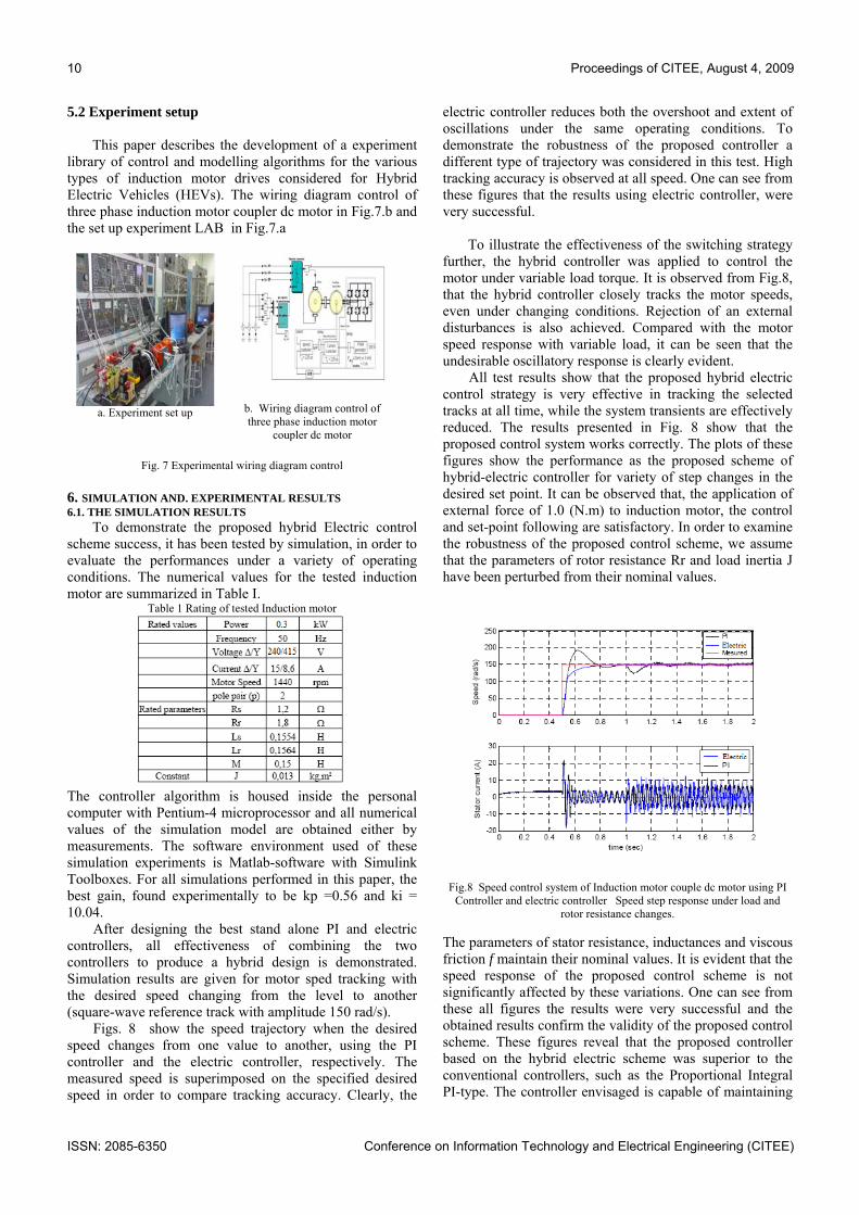
5.2 Experiment setup This paper describes the development of a experiment library of control and modelling algorithms for the various types of induction motor drives considered for Hybrid Electric Vehicles (HEVs). The wiring diagram control of three phase induction motor coupler dc motor in Fig.7.b and the set up experiment LAB in Fig.7.a

a. Experiment set up

b. Wiring diagram control of three phase induction motor

coupler dc motor

Fig. 7 Experimental wiring diagram control 6. SIMULATION AND. EXPERIMENTAL RESULTS 6.1. THE SIMULATION RESULTS To demonstrate the proposed hybrid Electric control scheme success, it has been tested by simulation, in order to evaluate the performances under a variety of operating conditions. The numerical values for the tested induction motor are summarized in Table I.

Table 1 Rating of tested Induction motor

The controller algorithm is housed inside the personal computer with Pentium-4 microprocessor and all numerical values of the simulation model are obtained either by measurements. The software environment used of these simulation experiments is Matlab-software with Simulink Toolboxes. For all simulations performed in this paper, the best gain, found experimentally to be kp =0.56 and ki = 10.04.

After designing the best stand alone PI and electric controllers, all effectiveness of combining the two controllers to produce a hybrid design is demonstrated. Simulation results are given for motor sped tracking with the desired speed changing from the level to another (square-wave reference track with amplitude 150 rad/s).

Figs. 8 show the speed trajectory when the desired speed changes from one value to another, using the PI controller and the electric controller, respectively. The measured speed is superimposed on the specified desired speed in order to compare tracking accuracy. Clearly, the

electric controller reduces both the overshoot and extent of oscillations under the same operating conditions. To demonstrate the robustness of the proposed controller a different type of trajectory was considered in this test. High tracking accuracy is observed at all speed. One can see from these figures that the results using electric controller, were very successful. To illustrate the effectiveness of the switching strategy further, the hybrid controller was applied to control the motor under variable load torque. It is observed from Fig.8, that the hybrid controller closely tracks the motor speeds, even under changing conditions. Rejection of an external disturbances is also achieved. Compared with the motor speed response with variable load, it can be seen that the undesirable oscillatory response is clearly evident. All test results show that the proposed hybrid electric control strategy is very effective in tracking the selected tracks at all time, while the system transients are effectively reduced. The results presented in Fig. 8 show that the proposed control system works correctly. The plots of these figures show the performance as the proposed scheme of hybrid-electric controller for variety of step changes in the desired set point. It can be observed that, the application of external force of 1.0 (N.m) to induction motor, the control and set-point following are satisfactory. In order to examine the robustness of the proposed control scheme, we assume that the parameters of rotor resistance Rr and load inertia J have been perturbed from their nominal values.

Fig.8 Speed control system of Induction motor couple dc motor using PI Controller and electric controller Speed step response under load and

rotor resistance changes. The parameters of stator resistance, inductances and viscous friction f maintain their nominal values. It is evident that the speed response of the proposed control scheme is not significantly affected by these variations. One can see from these all figures the results were very successful and the obtained results confirm the validity of the proposed control scheme. These figures reveal that the proposed controller based on the hybrid electric scheme was superior to the conventional controllers, such as the Proportional Integral PI-type. The controller envisaged is capable of maintaining



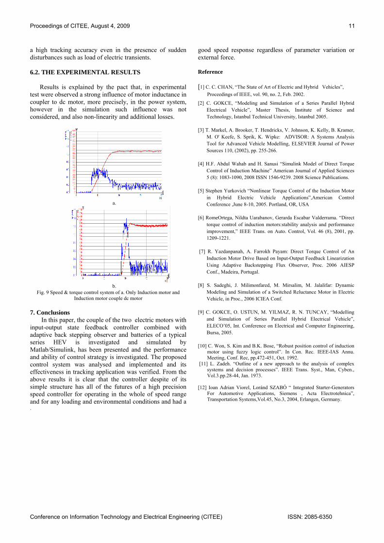
a high tracking accuracy even in the presence of sudden disturbances such as load of electric transients. 6.2. THE EXPERIMENTAL RESULTS Results is explained by the pact that, in experimental test were observed a strong influence of motor inductance in coupler to dc motor, more precisely, in the power system, however in the simulation such influence was not considered, and also non-linearity and additional losses.

a.

b.

Fig. 9 Speed & torque control system of a. Only Induction motor and Induction motor couple dc motor

7. Conclusions In this paper, the couple of the two electric motors with input-output state feedback controller combined with adaptive back stepping observer and batteries of a typical series HEV is investigated and simulated by Matlab/Simulink, has been presented and the performance and ability of control strategy is investigated. The proposed control system was analysed and implemented and its effectiveness in tracking application was verified. From the above results it is clear that the controller despite of its simple structure has all of the futures of a high precision speed controller for operating in the whole of speed range and for any loading and environmental conditions and had a

good speed response regardless of parameter variation or external force. Reference

[1] C. C. CHAN, “The State of Art of Electric and Hybrid Vehicles”, Proceedings of IEEE, vol. 90, no. 2, Feb. 2002.

[2] C. GOKCE, “Modeling and Simulation of a Series Parallel Hybrid Electrical Vehicle”, Master Thesis, Institute of Science and Technology, Istanbul Technical University, Istanbul 2005.

[3] T. Markel, A. Brooker, T. Hendricks, V. Johnson, K. Kelly, B. Kramer, M. O' Keefe, S. Sprik, K. Wipke: ADVISOR: A Systems Analysis Tool for Advanced Vehicle Modelling, ELSEVIER Journal of Power Sources 110, (2002), pp. 255-266.

[4] H.F. Abdul Wahab and H. Sanusi “Simulink Model of Direct Torque Control of Induction Machine” American Journal of Applied Sciences 5 (8): 1083-1090, 2008 ISSN 1546-9239. 2008 Science Publications.

[5] Stephen Yurkovich “Nonlinear Torque Control of the Induction Motor in Hybrid Electric Vehicle Applications”,American Control Conference ,June 8-10, 2005. Portland, OR, USA

[6] RomeOrtega, Nildta Uarabanov, Gerarda Escabar Valderrama. “Direct torque control of induction motors:stability analysis and performance improvement,” IEEE Trans. on Auto. Control, Vol. 46 (8), 2001, pp. 1209-1221.

[7] R. Yazdanpanah, A. Farrokh Payam: Direct Torque Control of An Induction Motor Drive Based on Input-Output Feedback Linearization Using Adaptive Backstepping Flux Observer, Proc. 2006 AIESP Conf., Madeira, Portugal.

[8] S. Sadeghi, J. Milimonfared, M. Mirsalim, M. Jalalifar: Dynamic Modeling and Simulation of a Switched Reluctance Motor in Electric Vehicle, in Proc., 2006 ICIEA Conf.

[9] C. GOKCE, O. USTUN, M. YILMAZ, R. N. TUNCAY, “Modelling and Simulation of Series Parallel Hybrid Electrical Vehicle”, ELECO’05, Int. Conference on Electrical and Computer Engineering, Bursa, 2005.

[10] C. Won, S. Kim and B.K. Bose, “Robust position control of induction motor using fuzzy logic control”. In Con. Rec. IEEE-IAS Annu. Meeting, Conf. Rec, pp.472-451, Oct. 1992.

[11] L. Zadeh. “Outline of a new approach to the analysis of complex systems and decision processes”. IEEE Trans. Syst., Man, Cyben., Vol.3.pp.28-44, Jan. 1973.

[12] Ioan Adrian Viorel, Loránd SZABÓ “ Integrated Starter-Generators

For Automotive Applications, Siemens , Acta Electrotehnica”, Transportation Systems,Vol.45, No.3, 2004, Erlangen, Germany.

.



Transient Stability of SMIB: a Case Study

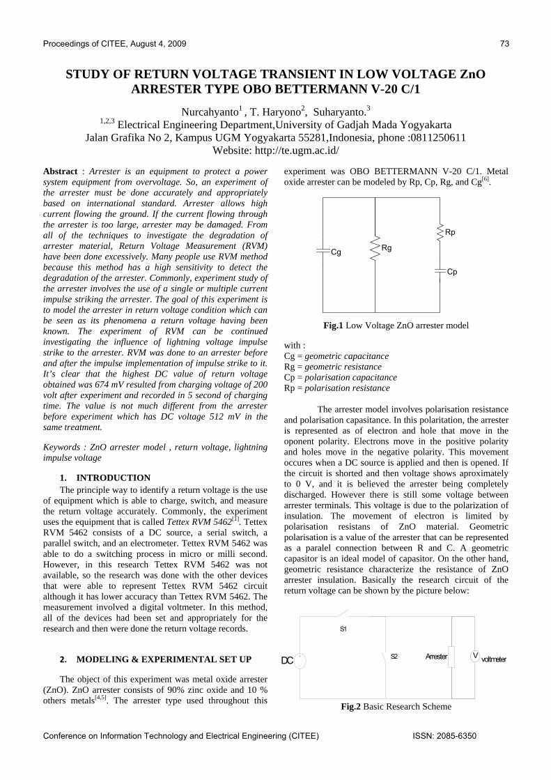
Adelhard Beni Rehiara Engineering Department, University of Papua (UNIPA)

Jl. Gunung Salju Manokwari, 98314, Indonesia email : [email protected]

Abstract— Single machine infinity bus (SMIB) is a simple way to examine a complex electrical power system. In investigating the transient stability of a SMIB system, equal area criterion (EAC) method can be used to get critical clearing angle δcr and critical clearing time tcr. In each case of a SMIB, critical clearing time tcr cannot directly be determined using equal area criterion method. This paper will introduce Runge-Kutta method utilized to modify the critical clearing time tcr found with EAC method and to know the best time to clear a fault. In this case, the critical clearing time tcr of EAC method is almost same for every fault and it is faster than the critical clearing time tcr of Runge-Kutta method.

Keywords— Transient stability, single machine infinity bus, equal area criterion, Runge-Kutta, step by step.

I. INTRODUCTION Electrical power systems consist of generation,

transmission and distribution system and/or also load as the user of the electrical power. The other components that can probably be connected to the systems are transformer, circuit breaker, relay protection, prime mover, etc. All of the power system components are used to maintain the quality, continuity, stability and reliability of the systems.

SMIB (single machine infinite bus) is a simple electrical power system that has a generator connected to infinite bus as load [11]. To make it simple to be analyzed, an interconnection electrical power system can be separated into some SMIBs.

Stability is an important constraint in power system operation [2]. The major problem in every electrical power system is how stability of the system when a fault happens for example short circuit, broken line, disconnected load, etc.

Equal area criterion (EAC) is a classic method in transient stability that is applicable to all two machines systems (SMIB). The method provides an easier way to determine the critical clearing angle δcr but the method does not able to find directly the critical clearing time tcr [4],[13]. Another mathematical calculation, called Runge-Kutta methods, will be used to solve the limitation of the EAC methods. This paper will combine both EAC and Runge-Kutta methods to get the best critical clearing time tcr.

II. TRANSIENT STABILITY

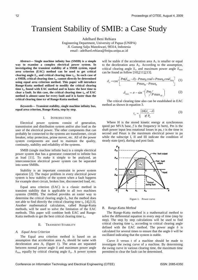
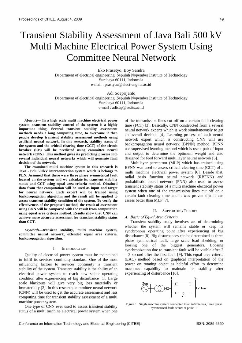
A. Equal Area Criterion The Equal area criterion method is based on an

assumption that acceleration area A1 should be same with deceleration area A2 (figure 1). The areas are separated between normal power angle δ and maximum power angle δmax equally by critical clearing angle δcr. A power system

will be stable if the acceleration area A1 is smaller or equal to the deceleration area A2. According to the assumption, critical clearing angle δcr and maximum power angle δmax can be found as follow [10],[11],[13].

⎥⎦

⎤⎢⎣

⎡−

+−−= −

IIIII

IIIIIcr PP

PPPmmaxmax

cosmaxcosmax)(cos maxmax1 δδδδ

δ (1)

⎟⎠⎞⎜

⎝⎛−= −

IIIPPm

maxsin 1max πδ (2)

The critical clearing time also can be established in EAC method as shown in equation 3.

( )m

crcr Pf

Ht

πδδ −

=2 (3)

Where H is the stored kinetic energy at synchronous speed per MVA base, f is the frequency in hertz, Pm is the shaft power input less rotational losses in pu, t is the time in second and Pmax is the maximum electrical power in pu while the subscript I, II and III indicate the condition of steady state (pre), during and post fault.

Figure 1. Power curve

B. Runge-Kutta Method The Runge-Kutta method is a mathematical method to

solve the differential equation in every step of time (step by step). The step by step calculations will be used to find critical clearing time tcr according to critical clearing angle defined with the EAC method. The power angle δ is calculated for several times to ensure that the angle δ will be oscillated indicating that the system is stable.

Curve δ versus t of a machine should be made to investigate the swing curve of a machine. By determining the swing curve in various clearing time, the maximum time permitted to clear the fault can be determined.



Some numeric methods, which are often used to solve the differential equation of step by step calculation, are the methods of Euler, Heun, Runge-Kutta, etc. In this case, it will be focused on the method of Runge-Kutta.

Fourth order of Runge-Kutta method can be utilized to analyze the swing equation. The equation can be rewritten as [3],[6]:

sdt

d ωωδ−=

( ) aem PH

PPHdt

d22ωωω

=−= (4)

Where Pe is the electrical power in pu, Pa is the accelerating power in pu and ω is the angular displacement of the rotor in rad. By substituting the swing equation to the method of Runge-Kutta, four estimations can be obtained [6].

First estimation:

( )k ddt

t tit

t s1 = = −δ

ω ω( )

( )Δ Δ (5)

( )l ddt

t fH

Pm Pe tit

t11= = −

ω π

( )( )( )Δ Δ (6)

Second estimation:

kl

ti ti

s212

= +⎛⎝⎜

⎞⎠⎟−

⎧⎨⎩

⎫⎬⎭

ω ω( ) Δ (7)

( )l fH

Pm Pe ti t22= −

π( )( ) Δ (8)

Third estimation:

kl

ti ti

s322

= +⎛⎝⎜

⎞⎠⎟−

⎧⎨⎩

⎫⎬⎭

ω ω( ) Δ (9)

( )l fH

Pm Pe ti t33= −

π( )( ) Δ (10)

Fourth estimation:

( ) k l ti t i s4 3= + −ω ω( ) Δ (11)

( )l fH

Pm Pe ti t44= −

π( )( ) Δ (12)

Where i = 1, 2, 3, ... , n and in the end of the period, the power angle δ and the synchronous speed ω will be changed using both equations below.

( ) ( )iiilittt kkkki 432)( 2261 ++++=Δ+ δδ (13)

( ) ( )iiilittt llll 432)( 2261 ++++=Δ+ ωω (14)

The calculation will be continued for t=t+Δt until the required duration of time. Critical clearing time tcr can be estimated using a linear interpolation method, which is formulated as [1]:

( ) tttcc

cccccr Δ

−−+

+=+

+

δδδδδ

1

121

(15)

Where tc and tc+1 are the time for clearing and after clearing fault while δc and δc+1 are the angle at clearing and after clearing fault.

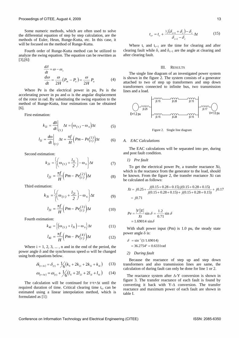
III. RESULTS The single line diagram of an investigated power system

is shown in the figure 2. The system consists of a generator attached to two of step up transformers and step down transformers connected to infinite bus, two transmission lines and a load.

j0.25 j0.17

E=1.2 pu V=1.0 pu

j0.15 j0.15j0.28

j0.15 j0.15j0.28

Figure 2. Single line diagram

A. EAC Calculations

The EAC calculations will be separated into pre, during and post fault condition.

1) Pre fault

To get the electrical power Pe, a transfer reactance Xt, which is the reactance from the generator to the load, should be known. From the figure 2, the transfer reactance Xt can be calculated as follows:

71.0

17.0)15.028.015.0()15.028.015.0(

)15.028.015.0()15.028.015.0(25.0

j

jjj

jjjXt

=

++++++++++

+=

δ

δδ

sin 1.69014

sin71.02.1sin

=

==Xt

EVPe

With shaft power input (Pm) is 1.0 pu, the steady state power angle δ is:

rad0.63312754.36)69014.1/1(sin 1

=°== −δ

2) During fault

Because the reactance of step up and step down transformers and also transmission lines are same, the calculation of during fault can only be done for line 1 or 2.

The reactance system after Δ-Y conversion is shown in figure 3. The transfer reactance of each fault is found by converting it back with Y-Δ conversion. The transfer reactance and maximum power of each fault are shown in table I.



j0.25 j0.17

E=1.2 pu V=1.0 pu

j0.0556 j0.2150

j0.0750

j0.25 j0.17

E=1.2 pu V=1.0 pu

j0.0145 j0.145

j0.0725

j0.25 j0.17

E=1.2 pu V=1.0 pu

j0.0556 j0.0750

j0.0250

(a) Front line fault

(b) Midle line fault

(c) End line fault

Figure 3. Δ-Y conversion

3) Post fault

When the fault is cleared, the system is operated by using a line. So the transfer reactance Xt and electric power Pe will be changed and those can be calculated as:

Xt = j0.25 + j0.15 + j0.28 + j0.15 + j0.17 = j1.0 Pe = 1.2 sin δ

The maximum power angle δmax and the critical clearing angle are:

( )rad2.1565

2.11sin 1

max

=

−= −πδ

°==

⎥⎦⎤

⎢⎣⎡

−+−−

= −

47.8529rad0.8351914054.02.1

1565.2cos2.16331.0cos4054.0)6331.01565.2(1cos 1crδ

In EAC method, the critical clearing time tcr is offered with equation 3 and the result for fault in front line is:

( )

s

tcr

101.050

2764.368529.478

=

−=

π

Power angle δ of normal operation and maximum power Pmax of pre and post fault are same wherever the fault happens. Result of calculations for the EAC method is given in table I.

TABLE I. VARIABLES DEFINED WITH EAC METHOD

Variables Fault Location

Front Middle End Xt (pu) j2.960 j2.4262 j2.759 Pmax (pu) 0.4054 0.4946 0.4349

δcr (deg) 47.8529 49.1602 48.2543 tcr (s) 0.101 0.107 0.103

B. Step by Step Calculations

The system is assumed to work with frequency 50 Hz and H=4MJ/MVA and the iteration interval is 0.05s. For the first time the fault happens, the acceleration power Pa is not in synchronous. So the acceleration power Pa is the average of Pa pre and Pa during fault.

1) Fault in a front line

The step by step calculation was done in Matlab with several clearing times tc and it was presented in following figures.

0 0.5 1 1.5 2 2.5 30

20

40

60

80

100

120

140

160

180

time (s)

pow

er a

ngle

(deg

)

tc = 0.05stc = 0.10stc = 0.15stc = 0.30s

Figure 4. Curve of δ for fault in front line

0 0.5 1 1.5 2 2.5 3300

310

320

330

340

350

360

time (s)

sync

hron

ous

spee

d (ra

d)

tc = 0.05stc = 0.10stc = 0.15stc = 0.30s

Figure 5. Curve of ω for fault in front line

The results of the calculations are angle δ and synchronous speed ω as shown in the figure 4 and 5. Base on the figures, the best clearing time tc is about 0.1s because clearing time a step toward (0.15s) will make the system unstable. So the critical clearing time tcr is probably in between 0.1s and 0.15s.

2) Fault in a middle line

The calculation results of the middle line fault are figured on figure 5 and 6. The calculations were done with PeI=1.69 sin δ, PeII=0.4946 sin δ and PeIII=1.2 sin δ. With clearing time tc = 0.15s, the swing curve is wide but the system is still stable.



Based on the next figure 6 and 7, the best time to clear the fault in the middle line is in 0.15s. The system will be unstable for the next step.

0 0.5 1 1.5 2 2.5 30

20

40

60

80

100

120

140

160

180

time (s)

pow

er a

ngle

(deg

)

tc = 0.10stc = 0.15stc = 0.20stc = 0.30s

Figure 6. Curve of δ for fault in middle line

0 0.5 1 1.5 2 2.5 3300

310

320

330

340

350

360

time (s)

sync

hron

ous

spee

d (ra

d)

tc = 0.10stc = 0.15stc = 0.20stc = 0.30s

Figure 7. Curve of ω for fault in middle line

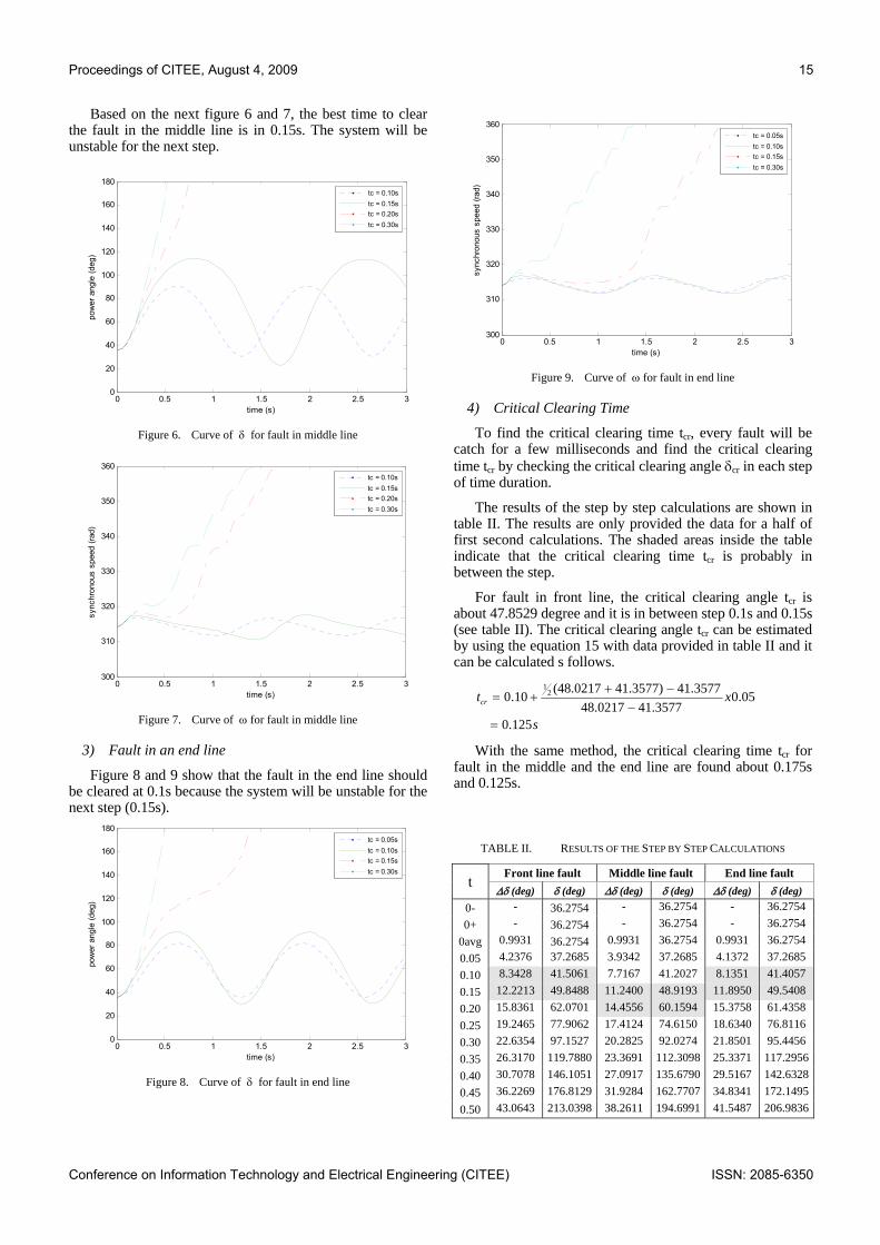
3) Fault in an end line

Figure 8 and 9 show that the fault in the end line should be cleared at 0.1s because the system will be unstable for the next step (0.15s).

0 0.5 1 1.5 2 2.5 30

20

40

60

80

100

120

140

160

180

time (s)

pow

er a

ngle

(deg

)

tc = 0.05stc = 0.10stc = 0.15stc = 0.30s

Figure 8. Curve of δ for fault in end line

0 0.5 1 1.5 2 2.5 3300

310

320

330

340

350

360

time (s)

sync

hron

ous

spee

d (ra

d)

tc = 0.05stc = 0.10stc = 0.15stc = 0.30s

Figure 9. Curve of ω for fault in end line

4) Critical Clearing Time

To find the critical clearing time tcr, every fault will be catch for a few milliseconds and find the critical clearing time tcr by checking the critical clearing angle δcr in each step of time duration.

The results of the step by step calculations are shown in table II. The results are only provided the data for a half of first second calculations. The shaded areas inside the table indicate that the critical clearing time tcr is probably in between the step.

For fault in front line, the critical clearing angle tcr is about 47.8529 degree and it is in between step 0.1s and 0.15s (see table II). The critical clearing angle tcr can be estimated by using the equation 15 with data provided in table II and it can be calculated s follows.

s

xtcr

0.125

05.041.357748.0217

41.357741.3577)(48.021710.0 21

=−

−++=

With the same method, the critical clearing time tcr for fault in the middle and the end line are found about 0.175s and 0.125s.

TABLE II. RESULTS OF THE STEP BY STEP CALCULATIONS

t Front line fault Middle line fault End line fault Δδ (deg) δ (deg) Δδ (deg) δ (deg) Δδ (deg) δ (deg)

0- - 36.2754 - 36.2754 - 36.2754 0+ - 36.2754 - 36.2754 - 36.2754

0avg 0.9931 36.2754 0.9931 36.2754 0.9931 36.2754 0.05 4.2376 37.2685 3.9342 37.2685 4.1372 37.2685 0.10 8.3428 41.5061 7.7167 41.2027 8.1351 41.4057 0.15 12.2213 49.8488 11.2400 48.9193 11.8950 49.5408 0.20 15.8361 62.0701 14.4556 60.1594 15.3758 61.4358 0.25 19.2465 77.9062 17.4124 74.6150 18.6340 76.8116 0.30 22.6354 97.1527 20.2825 92.0274 21.8501 95.4456 0.35 26.3170 119.7880 23.3691 112.3098 25.3371 117.29560.40 30.7078 146.1051 27.0917 135.6790 29.5167 142.63280.45 36.2269 176.8129 31.9284 162.7707 34.8341 172.14950.50 43.0643 213.0398 38.2611 194.6991 41.5487 206.9836



IV. CONCLUSSIONS Critical clearing time tcr found with EAC method is

almost same for the investigated system wherever the fault happens. For each fault in the system, the critical clearing angle δcr is different because the electrical power Pe for every fault is different. The difference also makes an influence for the critical clearing time tcr.

Using Runge-Kutta method, critical clearing angle δcr can not be used to define the critical clearing time tcr because the calculation using step by step is never exactly match with the critical clearing angle δcr. In this case, the critical clearing time tcr can be found with a linear interpolation method.

The result shows that the critical clearing time tcr defined with EAC method is faster than with Runge-Kutta method. Some differences appear in the result but both EAC and Runge-Kutta methods prove that the critical clearing time tcr is longer for every fault in the middle line.

REFERENCES [1] Achmad Basuki, ”Metode Numerik dan Algoritma Komputansi,”

Andi Offset, Yogyakarta, 2004. [2] Deqiang Gan, Robert J. Thomas, Ray D. Zimmerman, “A Transient

Stability Constrained Optimal Power Flow,” Bulk Power System

Dynamics and Control IV – Restructuring, Santorini, Greece, August 24-28, 1998.

[3] E. W. Kimbark, “Power System Stability,” vol. 2, John Wiley and Sons, Inc., New York, 1995.

[4] Elhawary, Mohamed E., “Electrical Power Systems; Design and Analysis”, Reston Publishing, Reston VA, 1995.

[5] Fitzgerald, A.E.Kingsley, C. Umans, “Mesin-Mesin Listrik,” Erlangga, Jakarta, 1997.

[6] Glenn W. Stagg, Ahmed H. Abiad, “Computer Method in Power System Analysis,” McGraw-Hill, 8th. edition, Kogakusha, 1984.

[7] Khan, “A PC Based Software Package for The Equal area Criterion of Power System Transient Stability,” IEEE Trans. Power System, Vol. 13, No. 1, Feb. 1998.

[8] M.A.Pai, “Computer Techniques in Power System Analysis,” Tata McGraw-Hill, New Delhi, 2006.

[9] Mohammad Reza, “A Survey on the Transient Stability of Power Systems with Converter Connected Distributed Generation,” Jurnal Teknik Elektro Vol. 7, No. 1, March 2007.

[10] Nagrath, D.P. Kothari, “Modern Power System Analysis,” second edition, Tata McGraw-Hill, New Delhi, 2001.

[11] Prabha Kundur, “Power system Analysis,” Tata McGraw-Hill, New Delhi, 1994.

[12] Shengli Cheng, Mohindar S. Sachdev5, “Out-of-Step Protection Using the Equal Area Criterion,” IEEE CCECE/CCGEI, Saskatoon, May 2000.

[13] William D. Stevenson Jr, “Analisis Sistem Tenaga Listrik,” Erlangga, Jakarta, 1996.



LOOK-UP TABLE OF FUZZY RULE SURAM WITH AVR ATmega128

Zakarias Situmorang

Faculty of Computer Science, Catholic University of Saint Thomas Medan Jl. Setiabudi No. 479-F Tanjungsari Medan 20132

Email : [email protected]

ABSTRACT Implemented of fuzzy rule must used a look-up table as defuzzification analysis. Look-up table is the actuator plant to doing the value of fuzzification. Rule suram based of fuzzy logic with variables of weather is temperature ambient and conditions of air is humidity ambient, it implemented for wood drying process. The membership function of variable of state represented in error value and change error with typical map of triangle and map of trapezium. Result of analysis to reach 8 fuzzy rule in 150 conditions to control the output system can be constructed in a number of way of weather and conditions of air. It used to minimum of the consumption of electric energy by heater. One cycle of schedule drying is a serial of condition of chamber to process as use as a wood species. Design in control used a AVR Atmega-128 as has a memory very big to apply a source code of a wood process schedule of drying.

keywords : look-up table, defuzzification, fuzzy controller, a wood schedule of drying, AVR Atmega-128

Introduction

The wood drying process used the schedule of drying dependent for moisture of content the wood, that condition of kiln in temperature and humidity of chamber. The controller used to control the actuators are heater, sprayer and damper, whenever the process used doing the optimal from time and energy and stability in wood schedule of drying. Main source of energy is solar energy from collector and alternative source energy by heater. Number of solar energy based of intensity of solar and alternative energy by heater is consumption of electric.

The maximized use of solar energy in wood drying process is goal of control system. It’s depended by a number solar energy and it’s change and temperature of ambient. Responsibility of the change the solar energy in variable of temperature ambient and humidity ambient is the especial of goal the control system. The process of control is to hope maximized the use of solar energy and the minimized of consumption energy of electric.

Process of wood drying is depended for schedule drying, which used to track of set point for temperature and humidity drying. The conditions of temperature and humidity drying in schedule are different for the each steps of the schedule drying of wood. Variable control the Wood drying of process kiln are temperature and humidity of air in

chamber where dependent for moisture of content the wood. It’s need to control of actuator system for heater, sprayer and damper, whenever the process used doing the optimal from time and energy and the actuator doing in the conditions data riel.

The Fuzzy rule suram implemented for schedule drying of Albasia Albizia wood and modification of membership function in range [0.5, 1].

Wood Drying Process

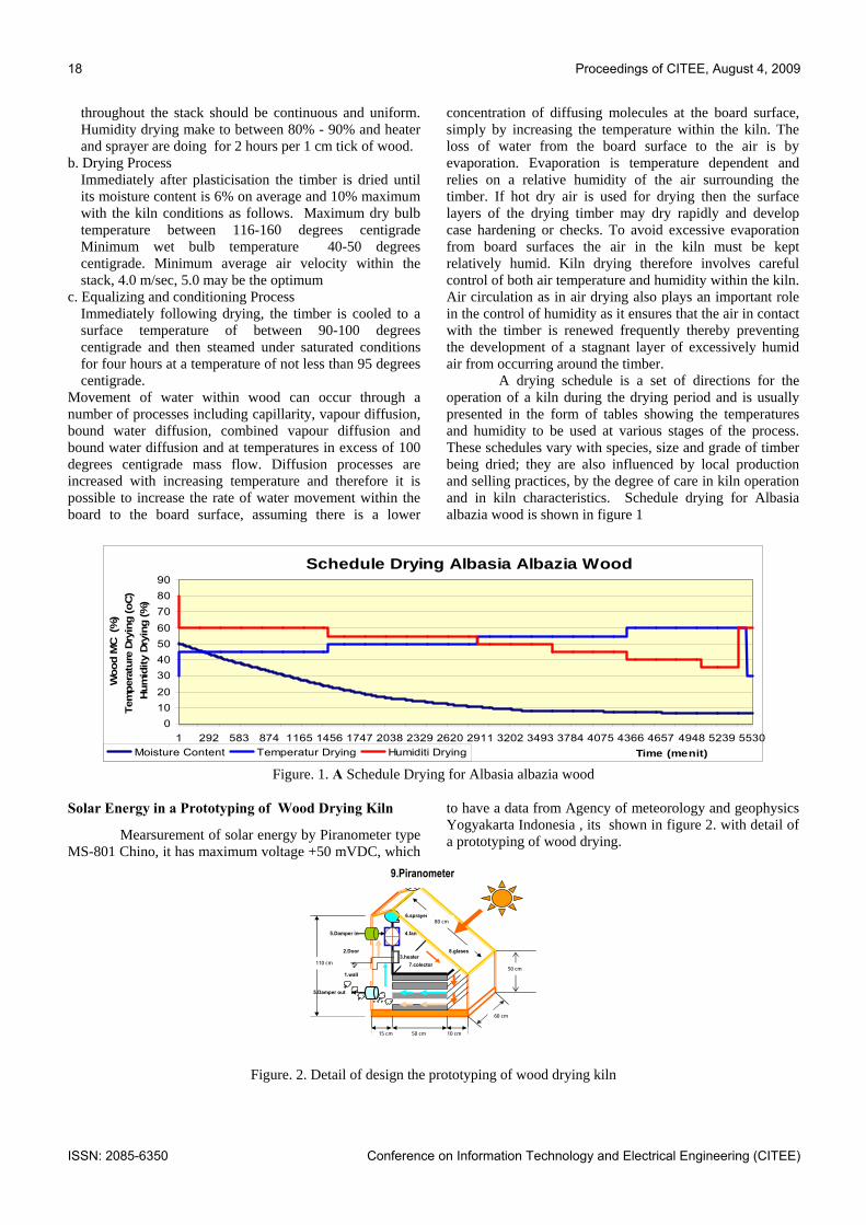
Control variable of a solar energy wood drying process kiln is temperature and humidity to adapt variable of a drying schedule. Dimension of wood drying kiln has designed and built several type dry kiln for use lumber of housing structure. The Schedule drying is a cycle of drying and have the some level of process. A Level process doing at temperature and humidity variable are constant at set point any time. By the way need an actuator control system (heater, sprayer and damper) then doing at effective the time and efficiency of energy.

Air drying involves the open piling of freshly processed timber in stacks out of doors or in open sheds so that the wood surfaces are exposed to the surrounding atmosphere. During air drying there is little control over the factors that influence drying and hence the rate of drying is very much controlled by local atmospheric conditions. One guiding principle during air drying of timber is to ensure adequate air circulation through the stack. In practice this is achieved by separating each board within the stack using sticks or stickers

High temperature drying, ie., drying above the boiling point of water, is the dominant method for the drying of radiata pine (Industry Standard 100-1992). The method which is used to dry wood in chamber with some level process is described below; a. Pre-Heating Process

This process describe to stability of temperature distributed in wood stacks is equally. . The rate of drying can be controlled to some extent by altering the size of the sticks. Drying can be slowed by using thinner sticks or increased by using wider sticks. During air drying, air circulating within the stack absorbs moisture, is cooled and in this process drops to the bottom of the stack. If a space or chimney is constructed within the centre of the stack then this cooler air can exit the stack and fresh air will be drawn in at the top of the stack. If this process occurs correctly then air movement and drying



throughout the stack should be continuous and uniform. Humidity drying make to between 80% - 90% and heater and sprayer are doing for 2 hours per 1 cm tick of wood.

b. Drying Process Immediately after plasticisation the timber is dried until its moisture content is 6% on average and 10% maximum with the kiln conditions as follows. Maximum dry bulb temperature between 116-160 degrees centigrade Minimum wet bulb temperature 40-50 degrees centigrade. Minimum average air velocity within the stack, 4.0 m/sec, 5.0 may be the optimum

c. Equalizing and conditioning Process Immediately following drying, the timber is cooled to a surface temperature of between 90-100 degrees centigrade and then steamed under saturated conditions for four hours at a temperature of not less than 95 degrees centigrade.

Movement of water within wood can occur through a number of processes including capillarity, vapour diffusion, bound water diffusion, combined vapour diffusion and bound water diffusion and at temperatures in excess of 100 degrees centigrade mass flow. Diffusion processes are increased with increasing temperature and therefore it is possible to increase the rate of water movement within the board to the board surface, assuming there is a lower

concentration of diffusing molecules at the board surface, simply by increasing the temperature within the kiln. The loss of water from the board surface to the air is by evaporation. Evaporation is temperature dependent and relies on a relative humidity of the air surrounding the timber. If hot dry air is used for drying then the surface layers of the drying timber may dry rapidly and develop case hardening or checks. To avoid excessive evaporation from board surfaces the air in the kiln must be kept relatively humid. Kiln drying therefore involves careful control of both air temperature and humidity within the kiln. Air circulation as in air drying also plays an important role in the control of humidity as it ensures that the air in contact with the timber is renewed frequently thereby preventing the development of a stagnant layer of excessively humid air from occurring around the timber.

A drying schedule is a set of directions for the operation of a kiln during the drying period and is usually presented in the form of tables showing the temperatures and humidity to be used at various stages of the process. These schedules vary with species, size and grade of timber being dried; they are also influenced by local production and selling practices, by the degree of care in kiln operation and in kiln characteristics. Schedule drying for Albasia albazia wood is shown in figure 1

Schedule Drying Albasia Albazia Wood

0102030405060708090

1 292 583 874 1165 1456 1747 2038 2329 2620 2911 3202 3493 3784 4075 4366 4657 4948 5239 5530Time (menit)

Woo

d M

C (

%)

Tem

pera

ture

Dry

ing

(oC

) H

umid

ity D

ryin

g (%

)

Moisture Content Temperatur Drying Humiditi Drying

Figure. 1. A Schedule Drying for Albasia albazia wood

Solar Energy in a Prototyping of Wood Drying Kiln

Mearsurement of solar energy by Piranometer type MS-801 Chino, it has maximum voltage +50 mVDC, which

to have a data from Agency of meteorology and geophysics Yogyakarta Indonesia , its shown in figure 2. with detail of a prototyping of wood drying.

Figure. 2. Detail of design the prototyping of wood drying kiln

50 cm

50 cm 10 cm 15 cm

80 cm

60 cm

8.glases

5.Damper in

±3.heater

6.sprayer

5.Damper out

110 cm

4.fan

7.colector

1.wall

2.Door

9.Piranometer



Most important part of a dehumidifying kiln is a heat pump. Air in the kiln passes through the load of timber and absorbs moisture from the wood. Part of that air circulates through the heat pump where the moisture is condensed and drained out of the chamber. Dried, reheated air comes back to kiln chamber. Energy consumption is

minimal, since there is almost no inner/outer air exchange. Air circulation in these kilns is smaller than in conventional kilns while the electrical power of flow fans and heat pump equals approximately the power of flow fans in conventional kilns.

A number of variable solar radiation can be convert to variable temperature ambient and humidity ambient shown in table 1.

Table. 1. Convert solar radiation to variable temp. ambient and humidity ambient for Albasia albizia wood.

No.

Set Point Td0 (oC)

Set Point Hd0 (%)

MC (%)

Solar Radiation

Io (Watt/m2)

Temp. Ambient Ta(oC) Hum. Ambient Ha (oC)

Min Rate Max Min Rate Max

1 2 3 4 6 7 8 9 10 11 12 1 45 60 25.5 - 50 561.0 29.1 30.1 31.1 52 60 68 2 50 55 10.4 – 25.5 662.0 29.7 30.7 31.7 46 54 62

3 55 50 7.8 – 10.4 763.0 30.5 31.5 32.5 40 48 56 45 7.3 – 7.8

4 60 40 6.7 – 7.3 617.5 29.4 30.4 31.4 50 58 66 35 6.4 – 6.7

5 65 (F)

60 6.3 - 6.4 535.0 28.9 29.9 30.9 54 62 70

Note : i. For MC ≥ 25 %,( Td0 = 45 s/d 55), The Solar Radiation )40(2.204600 −+= oTdI (watt/m2)

ii. For MC < 25 %,( Td0 = 60 s/d 70), The Solar Radiation )55(5.167000 −−= oTdI (watt/m2)

iii. Control priode for total used the energi from solar , )400(0003.01.0 0 −+= ICp (0C/menit) F = Fakultatif

Design Membership Functions

Design of membership function for variables in fuzzy logic implemented to mapp of typical of triangle and trapezium as of a drying schedule as shown in figure 1. and table 1 It’s needed to implemented control system of wood drying kiln.

Fuzzification of membership function in range [0.5, 1], and for weather (temperature of ambient Ta and change temperature ambient CTa) for set point temperature drying Td0 = 450C and Humidity drying Rd0 = 60%) describe by figure 3. with variable M : over-cloudy ; B : cloudy; CB : bright-cloud ; C: clear; SC : clearest and for change of temperature ambient used -H = - High, -M = -Medium, -S = - Small, Z = Zero, S = Small, M = Medium, H = High.

28.1 29.1 30.1 31.1 32.1 Ta(0C)

C SC B CB M

1

0.5

- 0.6 - 0.4 - 0.2 0 0.2 0.4 0.6 CTa(0C)

+S +H B Z-H +M -S -M

1

0.5

Figure. 3. Membership function of temperature ambient and

change temperature ambient for Td0 = 450C and Rd0 = 60%

Computation process of variable change of temperature ambient are given eq.1. with n → 0 s/d ∼

CTa [(n+1)T] = Ta[(n+1)T] – Ta[nT] (1)

Representative of weather is variable temperature ambient and this change used to maximize and to hoist responsibility of membership Function, with appropriate rule in a table look-up scheme, shown table 2.



Table 2. Look-up table for membership Function for temperature of ambient

Ta CTa

Over-cloudy (M) Cloudy (B)

Bright-Cloud (CB)

Clear (C)

Clearest (SC)

-H Over-cloudy Over-cloudy Cloudy Bright-Cloud Clear -M Over-cloudy Cloudy Bright-Cloud Clear Clearest -S Over-cloudy Cloudy Bright-Cloud Clear Clearest Z Over-cloudy Cloudy Bright-Cloud Clear Clearest +S Over-cloudy Cloudy Bright-Cloud Clear Clearest +M Over-cloudy Cloudy Bright-Cloud Clear Clearest +H Cloudy Bright-Cloud Clear Clearest Clearest

Fuzzyfikasi of membership function in range [0.5,

1] of conditions of air (humidity of ambient Ha and change of humidity ambient CHa) for set point temperature drying (Td0 = 450C) and humidity drying (Rd0 = 60%) describe by

figure 4. with variable : P : Hot; AP : Rather-Hot; H : Swarm; S: Fresh; D : Cold, and for change of humidity ambient used -H = - High, -M = -Medium, -S = - Small, Z = Zero, S = Small, M = Medium, H = High.

52 56 60 64 68

μB

Ha(%)

S D AP H P

0.5

1

- 3 - 2 - 1 0 1 2 3 CHa(%)

+S +H B Z-H +M -S -M

0.5

1

Figure. 4. Membership Function of humidity ambient and change humidity for Td0 = 450C and Rd0 = 60%

Computation process of variable change of humidity ambient are given eq.2. with n → 0 to ∼

CHa [(n+1)T] = Ha[(n+1)T] – Ha[nT] (2)

Representative of conditions of air in variable humidity ambient and this change used to maximum of membership function, with appropriate rule in a table look-up scheme, shown table 3. For other step will be to adjust at table 1. and adapt for schedule drying at figure 1

Table 3. Look-up table for membership Function for humidity of ambient Ha CHa

Hot Rather-Hots Swarm Fresh Cold

-H Hot Hot Rather-Hot Swarm Sejuk -M Hot Rather-Hot Swarm Fresh Cold -S Hot Rather-Hot Swarm Fresh Cold Z Hot Rather-Hot Swarm Fresh Cold +S Hot Rather-Hot Swarm Fresh Cold +M Hot Rather-Hot Swarm Fresh Cold +H Rather-Hot Swarm Fresh Cold Cold

Implementation Control System

Automatic control unit has built-in programs for drying of all wood types regardless of a starting wood moisture content. It controls drying process automatically, so the operator presence is not needed during drying. Larger energy consumption is only during first day during heating stage when electrical heaters are turned on until

working temperature is reached. Later, during drying stage these heaters are rarely turn on. If a boiler installation exists in the drying complex, it makes sense to mount heat exchangers for hot water or steam (depending on the boiler) in the kiln. In that case, energy from the boiler would be used for heating of the drying chamber. That way kiln becomes combined (automatically uses boiler heat). This option is interesting only for a large



capacity kilns and in the cases where electrical power supply is unstable (large voltage or current oscillation or frequent power cut-downs during winter periods). Drying is in that case performed in conventional way, heat pump is turned-off, and electrical energy is used only for flow fans. Combined kiln unites good characteristics of both dehumidifying and conventional kiln. That provides the greatest drying quality with the least energy consumption for the shortest time.

Drying quality in dehumidifying kilns is significantly better than in any conventional kiln, because the drying is equable in whole timber load, so there is no

danger of developing degrade in the timber (cracks, checks, warping...). drying is fast enough since the working temperature can reach up 60 0C to. These kilns are environment friendly because all wastes that are produced during drying process are harmless for water and environment. Especially good results are achieved with drying of natural (untreated) wood (beech, ash,...).

Input variable in measurement by SHT11-sensor and shown in figure 5. Schematic control system in figure 6 and flowchart fuzzy controlller illustrated at figure 7. In table 4 describe input variable. and output variable used to fuzzy rule suram shown at table 5

Figure.5. Control system for prototyping wood drying kiln

Microcontroller AVR Atmega 128 have a capacity

a big amount 128k flash, 53 pin I/O, 6 channel PWM and 8 channel ADC 10-bit; then to used for application system control complex. Microcontroller AVR Atmega 128 is a microcontroller AVR Atmel 8 bit family, with specification are : • 128 Kb Flash PEROM • 4Kb EEPROM, 4Kb SRAM • On Chip Analog Comparator • 8 Channel 10 bit ADC • 2 8 bit PWM • 6 PWM with resolution programmable (2-16 bit)

• Dual Programmable UART • SPI Interface • Programmable Watchdog with On Chip Oscillator • Adjustable VREF ADC • 53 bit I/O • Power On Reset dan Programmable Brown out

detection • Internal Calibrated RC Oscillator • The pocket included the cabel ISP, CD and cabel

RS232

Glass

Rd

Damper in

±

heater

sprayer

Damper out

fan

Ta

Microcontroller AVR Atmega 128

Td

RTC

Relay

Motor Stipper

Display 7 segmen

Ha

DISPLAY

on/off



Figure.6. Schematic fuzzy controller system

Tabel 4. Input variable

No. Variable Range Describe 1. Temperature Drying Td 0 – 150 0C 2. Temperature Ambient Ta 0 – 150 0C Weather 3. Humidity Drying Rd 0 – 100 % 4. Humidity Ambient Ha 0 – 100 % Conditions of air

Tabel 5. Output variable and implemented the fuzzy rule suram

No. Rule Actuator Conditions Heater Damper Sprayer

1. SUR-AM – 1 off off S To drop of Temperature Drying Td and to hoist of Humidity Drying Rd by very suddenly [Heating- Process]

2. SUR-AM – 2 H off off To hoist of Temperature Drying by very suddenly and to drop of humidity drying Rd.

3. SUR-AM – 3 H D3 off To hoist of Temperature Drying Td and to stay of Humidity Drying Rd.

4. SUR-AM – 4 H D2 S To hoist of Temperature Drying and to drop of humidity drying Rd.

5. SUR-AM – 5 H1 D3 off To drop of Temperature Drying Td and to stay of Humidity Drying Rd

6. SUR-AM – 6 H2 off S To drop of Temperature Drying Td and to drop of Humidity Drying Rd

7. SUR-AM – 7 off off off To stay of Temperature Drying Td and to stay of Humidity Drying Rd

8. SUR-AM – 8 H D1 off To stay of Temperature Drying Td and to adjust Humidity Drying Rd with Humidity ambient Ha [Equalizing-Process]

Note: D1 : Damper ON : 5 menit H : Heater ON : 15 menit D2 : Damper ON : 2 x 1 menit H1 : Heater ON : 10 menit D3 : Damper ON : 1 x 1 menit H2 : Heater ON : 5 menit S : Sprayer ON : 1 x 1 menit.



Figure.7. Flowcart fuzzy controller system

Result of Implementation the fuzzy rule suram for

measurement of temperature drying for schedule Albasia Albizia wood drying, with specification : wood dimension :

4 x 6 cm, amount : 22 item. The figure 8 and figure 9. shown , that measurement of temperature drying can be to follow schedule drying.

Measuremet of Temperature Drying and MC-wood 3-7 Juni 2008

010203040506070

11:23

14:47

11:26

14:50

18:14

21:38

1:02

4:26

7:50

11:14

14:38

18:02

21:26

0:50

4:14

7:38

11:02

14:26

17:50

21:14

0:38

4:02

7:26

time

Tempe

rature D

rying (oC)

MC W

ood (%

)

Figure 8. Measurement of temperature drying and MC-Wood at 3-7 Juni 2008

Measurement of Temperature Drying and MC-Wood 10-14 Juni 2008

0

10

20

30

40

50

60

70

9:40

12:22

15:04

17:46

20:28

23:10

1:52

4:34

7:16

9:58

12:40

15:22

18:04

20:46

23:28

2:10

4:52

7:34

10:16

12:58

15:40

18:22

21:04

23:46

2:28

5:10

7:52

10:34

13:16

15:58

18:40

21:22

0:04

2:46

5:28

Time

Tempe

rature D

rying (oC)

MC W

ood(%)

Figure 9. Measurement of temperature drying and MC-Wood at 10-14 Juni 2008

Temp. Drying MC Wood Set point Td

Temp. Drying MC Wood Set point Td



Conclusion Rule suram based of fuzzy logic with variables of weather is temperature ambient and conditions of air is humidity ambient, and it can implemented for wood drying process. The membership function of variable of state represented in error value and change error with typical of triangle and trapezium. Result from analysis and evaluation, the 8 fuzzy rule to control for output system can be constructed in a number of way of weather and conditions of air. It used to minimum of the consumption of electric energy by heater. The rule suram used to stability and equilibrium of schedule of drying in chamber by control of temperature and humidity. The result of implemented of fuzzy rule suram with the modification of membership function in range [0.5, 1] represented approximate to he conditions riel are near enough and the actuator doing in the conditions data riel Reference [1]. Nogueira, A., et all, Simulation and control strategies

for an energetically efficient wood drying process, EFITA/WCCA Joint Congress on IT in Agriculture, Vila Real Portugal, page 244 -251. 2005

[2]. Lim P.K.and Natalie R.S.,; Climate control of a storage chamber using fuzzy logic; Proceedings of the 2nd ANNES IEEE, 1995.

[3]. Virginia Tech, Virginia Cooperative Extension, Virginia State University,, Design Of Solar-Heated Dry Kiln, 2007

[4]. Kantay, R., Oner Unsal, Suleyman Korkut, 2002, Drying problems of fast growing tree species : Evaluation of Maritime pine (Pinus pinaster Alt) and Eucalyptus (Eucalyptus camaldulensis Dehn) wood., Proceedings International IUFRO Meeting Management of fast Growing Plantations, DIV.4.04.06,pp 208-212, 11th-13th September 2002, Izmit-Turkey

[5]. Wang L.X, A course in Fuzzy Systems and Control, Prentice-Hall International, Inc, 1997.

[6]. Joseph C.G and Gary D.R, Expert system Principle and Programming, Thomson Course Technoloy, Fourth Edition, Canada, 2005.

[7]. Klir, G.J, and Bo Yuan, Fuzzy sets and Fuzzy Logic Theory and Applications, , Prentice-Hall International, Inc, New York, 1995.

[8]. Duenas, A., and Dobrila P, A new Approach to Multi Objective Single-Machine Scheduling Problem under Fuzzines, Decision Support in an uncertain and complex word: the IPIP TC8/WG8.3. International Conference, 2004

[9]. Haque.M.N., Modelling of Solar Kilns and The Development of An Optimised Schedule for Drying Hardwood Timber, Thesis Ph.D., Department of Chemical Engineering, University of Sydney., 354p. 2002

[10]. Dion,J.M., L.Dugard, A.Pranco, N.M. Tri, J.W.Horwood., “MIMO Adaftive Constrained Predictive Control Case Study : An Environmental Test Chamber”, Automatica, 27, 1991, 611- 626, Pergamon-Press

[11] Garrahan.P., and Jeff Kidlark, 2001, Drying Hardwoods - Northern Hardwood Initiative : Industry Resource Manual, Forintek Canada Corp, 2665 East Mall, Vancauver, B.C. V6I 1W5.

[12] Sun, Z.F., C.G.Carrington., C.Davis, Q.Sun, and S.Pang, Drying Radiata Pine Timber under Dehumidifier Conditions : Comparison Of Modelled Results with Experimental Results, 8th nternational IUFRO Wood Drying Conference-2003 page 39 – 44

[13]. Laurenzi. W., V.Popa, Gh.Comsa, Computer Aided Design Of Drying Schedules In Order To Control The Drying Process, 8th International IUFRO Wood Drying Conference, 2003, 302 – 307.

[14] Nogueira, A., et all, 2005, Simulation and control strategies for an energetically efficient wood drying process, EFITA/WCCA Joint Congress on IT in Agriculture, Vila Real Portugal, 2005, 244 -251

[15] Skuratov. N.V., Computer Simulation and Dry Kiln Control, 8th International IUFRO Wood Drying Conference, 2003, 406 – 412

[16] Wang, X.G. Liu, W. Gu, L. Sun, C.J. Gu, C.E. de Silva, C.W., Development of An Intelligent Control System for wood drying proceeses , Advanced Intelligent Mechatronics Proceedings. 2001 IEEE/ASME International Conference. Vol.I, 2001, 371 – 376.

[17] Situmorang, Z., et all, The Schedule Of Optimal Fuzzy Controller Gain With Multi Model Concept for a Solar Energy wood Drying Process Kiln, International Journal Of Operations and Quantitative Management, 2009..



OPTIMAL CAPACITOR BANK LOCATION IN THE PRIMARY FEEDER WITH TYPICAL FLAT LOAD

Hermagasantos Zein

Department of Energy Conversion Technology, Bandung State Polytechnic Mail Box: Pos 1234, Indonesia

Email: hermaga_s @ Yahoo.co.id Mobile phone: 081321108991

.

Abstract- A capacitor bank is not only used for improving power factor, but can also be used to minimize losses in electric system networks. This paper is aimed to determine an optimal location of capacitor bank in the typical flat load of a primary feeder in order to get maximal losses-saving. The capacitor bank position will affect loss-saving depending on the number of nodes and the magnitude of compensation current generated by the capacitor bank. By simulation, the optimal position of capacitor bank from the substation is further than the center of feeder. For 100% compensation and unlimited number of nodes, the optimal location is 50% of feeder length. Optimal condition for 15 nodes, for 100% compensation is 0.53 pu and 30% compensation is 0.92 pu from the substation. Generally, the maximal saving occurs between 50% and 70% compensation, and the location of the capacitor bank unchanged for the number of nodes greater than 15. Then, the optimal locations for multi capacitor banks also depends on both the number of nodes and the magnitude of compensation current generated by every capacitor bank. For five capacitor banks with the number of nodes greater than 10 nodes indicate that the optimal locations of them are not changed for 15% compensation, i.e. 0.3 pu, 0.5 pu, 0.7 pu, 0.8 pu and 1.0 pu from the substation.

Keywords- bank capacitor, losses saving, primary feeder, optimal location

I. INTRODUCTION

An inductive load in the primary feeder will decrease

the power factor of system because it has to supply reactive power to the load. For feeders with low power factors (less than 89%) have to be corrected until the reactive supply become smaller. If the compensation is aimed only for correcting of the power factor of system, the capacitor bank location will be independently (no problem). Another problem appears while correcting the power factor, how much losses in the feeder can be reduced by installing of capacitor bank. It is possible because of the capacitor bank current will reduce reactive current produced by the load (as dominant contribution), so, the current flowing and losses in the feeder can be reduced. Significance of reducing in losses in the feeder is influenced by the location where the capacitor bank is installed. If losses reducing as consider in installation of capacitor bank in the feeder, the capacitor bank location have to be looked for in order to reduce losses

to be maximum. Where the losses in the distribution system (primary feeder is dominant) is greater than 60% from total losses system.

Figure-1 is a primary feeder with lumped load and current (I) flowing in the feeder. Supposed that resistance of the feeder is R, power factor ( φCosFb = ) lagging and reactance of the feeder is ignored, then, the current flowing in the feeder is also lagging with respect to the voltage by phase angleφ . The current can be formulated as

ra jIIjISinICosI

−=−=

φφ

(1)

where: φICosIa = is an active current

φISinIr = is a reactive current

Figure-1: The feeder with lumped load

From figure-1, losses can be derived from the equation-1 and yields:

RIIP rar )( 22 += (2) If at the load is installed the capacitor bank that yield current, Ic, losses in the feeder can be determined from the equation-2 and yield

RIIIII

RIIIP

ccrra

crac

r

]2[

])([222

22

+−+=

−+= (3)

From the last two equations, the saving power by installing capacitor bank is

22 ccr

crrr

III

PPP

−=

−=Δ (4)

From equation-4, the losses which can be saved and depend only on the reactive current. The active current is not shared in this case.



II. LOSSES REDUCTION BY THE CAPACITOR BANK

Figure-2 is the reactive current curve in the feeder. This curve is expressed as a function of distance (x) as:

)(xfI x= (5) Then, the losses can be counted in every segment with distance dx from the feeder in the figure-2 as:

')]([3 2 xLRxfPrr ∂=∂ (6)

Figure-2: Reactive current versus distance in

the feeder Therefore, total losses along feeder can be counted by integrating the equation-6 and resulting:

')]([30

2∫ ∂=L

rr xLRxfP (7)

where: Prr is total losses affected by reactive current. f(x) is reactive current function along feeder R is total resistance of feeder. L is total distance of feeder. dx’ is the distance element.

From figure-2, let x is the location of a unit capacitor bank from the substation and Ic is phase current of the bank, now the total losses is:

∫∫

∫∫

∫∫

∂−+=

∂+∂+−=

∂+∂−=

x

cc

L

L

x

x

cc

L

x

x

cc

rr

xxfIILRxf

LR

xxfLRxIxfIxf

LR

xxfLRxIxf

LRP

00

2

2

0

22

2

0

2

')](2[3)(3

')(3'])(2)([3

')(3'])([3

(8)

The last two equations is able to reduce losses in unit distance as:

xIxfRIPPPx

ccc

rrrrrr ∂−=−=Δ ∫ ])(2[30

(9)

where: dx=dx’/L From equation-9 can be determined the optimal location of the capacitor bank through derivative of the equition-9 to distance and the result is an optimal location (xm) as:

0])(2[3 =−=∂Δ∂

cmcrr IxfRI

xP

(10)

This equation can be simplified further as:

2)( c

mIxf = (11)

III. FEEDER WITH TYPICAL FLAT LOADS

Figure-3 is a feeder with the typical flat loads (10 nodes). The mathematical model of current function along the feeder is linear.

bxaxf +=)( (12)

Figure-3: A Feeder with typical flat loads

From equation-8 and equation-9, losses which can be saved depend on the location of a capacitor bank along the feeder. Let the location of a capacitor bank is x-distance from the substation, the losses can be determined as:

⎥⎦

⎤⎢⎣

⎡+

−=

+−=

∂−+=

∂−=−=Δ

∫∫

22

20

0

23

])2[(3

])(2[3

])(2[3

xIbx

IIa

IIRI

bxxIaRI

xIbxaRI

xIxfRIPPP

TT

c

T

cT

cc

x

cc

x

ccc

rrrrrr

And let the losses of one unit is 3 2TRI and TI/Ik c= ,

whereas nII T= , TIa = and LIIb t /)( −= , the power can be saved (losses saving) in the unit is

]1)2[()( 2xn

nxkkpuPrr−

−−=Δ (13)

For n=10, plots of equation-13 to k variation are presented in the figure-4. The figure points out that maximum saving of 0.33 pu accurs at k=0.7 (or capacitor bank compensation 70%) by distance x=0.7 pu. Whereas compensation 100%, maximum saving is 0.28 pu and the location between x=0.5 pu and x=0.6 pu. The optimal point goes down by increasing of of distance from x=0.5 pu to x=1.0 pu. Whereas the saved maximum power can be increased by reducing the compensation downs to 60% and it goes down again if the compensation ins increased. From the curve in the figure-4, the best compensation are at k=0.5, k=0.6 and k=0.7.



0.00

0.05

0.10

0.15

0.20

0.25

0.30

0.35

0 0.1 0.2 0.3 0.4 0.5 0.6 0.7 0.8 0.9 1

Jarak dari GI (x)

Loss

es s

avin

g (N

=10)

k=1,0

k=0.9

k=0.8k=0.7k=0.6

k=0.1

k=0.5

k=0.2

k=0.3

k=0.4

Figure-4: Losses saving curve versus

variation of capacitor bank location for n=10

IV. OPTIMAL LOCATION

From equation-11, the optimal location of the capacitor bank from the substation, xm, for flat load (figure-3) can be determined as:

)2

1(1

2

112

2 kn

nII

nn

bIax

T

ccm −

−=⎟⎟

⎠

⎞⎜⎜⎝

⎛−

−=

−= (14)

where: Tc IIk /= is capacitor current and reactive current ratio at supply.

n =2,3 … is number of loads in the feeder. The equation-14 points out that optimal location of a capacitor bank depends on the number of loads or nodes, n, and compensation capacity, k. Figure-5 is curves of optimal location for difference n and k. For the capacity of k, optimal distance becomes smaller when n is increasing at some extend then it becomes constant for further increasing of n. The optimal location x declines sharply for n less than 10 and for n greater than 10 nodes the decline is not significant (close to constant). Example for k=1 pu, x=0.556 pu and it will lead to x=0.5 pu on ∞=n and k=0.8 can be result x= 0.667 and it will lead to x=0.6 at ∞=n .

0.5

0.6

0.7

0.8

0.9

1.0

2 3 4 5 6 7 8 9 10 11 12 13 14 15 16 17 18 19n

x

k=1.0

k=0,9

k=0,1

k=0,3

k=0,2

k=0,4

k=0,5

k=0,6

k=0,7

k=0,8

Figure- 5: Optimal location of a capacitor bank

in the flat load feeder Then amount of saving that is gotten for optimal

location versus the number of nodes variation can be derived through equation-13 and equation-14, and it yields equation-15. It pointed that maximal saving only depend on n and k. Plot of the equation-15 is presented in the figure-6. It states that the influence of optimal location versus number of nodes for variation of compensation. It declines sharply from n=2 to n=10, and whereas for n>10 there is nearly no change in loss saving. Like that has been explained before, the good savings are for k=0.5 to k=0.7.

2

22

2

)2(1

25.0

])2(1

25.0)2(1

5.0[

]1)2[(

)2

1(1

1)2

1(1

)2()(

kn

nk

kn

nkn

nk

nnkk

kn

nn

nkn

nkkpuPmakrr

−−

=

−−

−−−

=

−−−=

⎥⎥⎦

⎤

⎢⎢⎣

⎡⎟⎠⎞

⎜⎝⎛ −

−−

−−−

−=Δ (15)

0.0

0.1

0.2

0.3

0.4

0.5

0.6

2 3 4 5 6 7 8 9 10 11 12 13 14 15 16 17 18 19 20n

Losses saving

k=0.1

k=1.0

k=0.3

Figure-6: Amount of power can be saved for a capacitor bank location versus n

V. FOR M-CAPACITOR BANK

Capacitor bank can be put in the feeder more than one unit. By assumption that m-capacitor banks are identically, the losses as consequence of the m-capacitor bank can be written as:

∫∫

∫∫

∫∫

∫

∫

∫∫

∂−++∂−−−

+∂−+=

∂++∂−+−−

+∂+−=

∂+

+∂−−+∂−=

x

cc

x

x cc

x

cc

L

L

x

x

x cc

x

cc

L

xm

x

x c

x

cc

rr

xxfIILRxxfmImI

LR

xxmfImILRxf

LR

xxfLRxImxfImxf

LR

xImxfmIxfLR

xxfLR

xImxfxmIxfLRP

0

2

1

2

1

0

2

0

2

22

1

222

1

0

222

2

2

1

21

0

2

')](2[3')]()1(2)1[(3

')](2[3)(3

')(3...'])1()()1(2)([3

'])(2)([3

')(3

...'])1()(['])([3

The saving can be counted such as a single unit that was explained before and it results:

...])2()()2(2[

])1()()1(2[

])1()()1(2[

])(2[3RI

])(2[3

...])1()()1(2[3

])(2[3

2

0

2

2

0

2

1

0

2

1

0

2c

2

1

2

1

0

2

+∂−−−

−∂−−−

+∂−−−

−∂−=

∂−+

+∂−−−

+∂−=Δ

∫∫∫

∫∫∫∫

xImxfm

xImxfm

xImxfm

xImxmf

xIxfRI

xImxfmRI

xImxmfRIP

x

c

x

c

x

c

x

c

L

m cc

x

x cc

x

ccrr

From the last equation , it can be simplified in term of unit as equation-16. This equation points out that the saving is also influenced by location of the capacitor bank-i.



im

m

i T

Cimx

T

crr x

IIixf

IIP

im

−+=

−+ ∂−−

=Δ ∑ ∫−+

11

1

0

)12()(21

(16)

VI. OPTIMAL LOCATION OF M-CAPACITOR BANK

Optimal location each capacitor bank can be found by of the equation-16 resulting:

0)12()(2 1 =−−−+ Cim Iixf (17)

Substitution the current function, f(x), then the optimal location each capacitor bank can be determined as loads in the equation-18.

)2

121(11 ki

nnx im

−−

−=−+ (18)

Equation-18 explains that the optimal location of

each capacitor bank depends only on the number of nodes and capacity of compensation applied. Table-1 gives results for 5 capacitor banks with compensation 15% each others from reactive current supply. For n>15 optimal location of each capacitor bank is constant. Significant changes occur between n=2 to n=6, for n=2: 4 capacitor bank at x=1.0 pu and one capacitor bank at x=0.7 pu. When it is compared to n=6: only one capacitor bank at x=1.0 pu and the others distributed in the feeder. Table-1: Optimal location of 5 capacitor bank in the

feeder for k=0.15 with variation of number of nodes

VII. ANALYSIS

Current in the flat load feeder (figure-3) declines

linearly by the increase of distance from substation to the end of feeder. The capacitor bank put in the flat load feeder is not only improving the power factor but also saving energy. The saving depends on location as consequence of the current change. The results of installing a capacitor bank states that maximal saving occur between compensation 50% to 70%, as presented in figure-4. Whereas optimal location varies with number of nodes and the compensation capacity applied. For indefinite number of nodes with compensation 100%, optimal location is at the center of feeder, it is optimal location with the shortest distance from substation. If n is reduced, the optimal location will become longer from half distance of feeder. Figure-5 points out that for n>15, the optimal location is nearly constant and it is found the same condition as is pointed by figure-6. For m-capacitor bank, optimal location of each capacitor banks depends on its compensation capacity. Table-1 points out that for n>10 nodes, optimal location each capacitor banks is close to constant. Whereas for n<5, lumped all of capacitor bank is occurred at the end of feeder (for n=5 is two capacitor banks and n=2 is four capacitor banks)

VIII. CONCLUSION

Capacitor bank position in feeder is truly determining saving which depends on the number of nodes or load location and capacity of current compensation produced the capacitor bank. The result in figure-4 shows than in flat load of feeder, the optimal location of a capacitor bank is in the center by unlimited number of nodes and 100% compensation. Whereas small compensation or equal reactive load current, the optimal location is at the end of feeder. So location of single capacitor bank will be between half distances to the end of feeder. Maximal saving of single capacitor bank with flat load is occurred on between compensation 50% and 70%.

Optimal location of single capacitor bank in the flat load feeder is not changed for number of nodes greater than 14. Thus, the saving is truly influenced by compensation capacity applied (figure-5), for full compensation (100%) optimal location is 0.53 pu from substation, and with compensation 30%, the location is at 0.92 pu from substation.

The optimal location for m-capacitor bank depends also on the number of nodes and compensation capacity applied. By simulation, for 5 capacitor bank with compensation 15% shows the optimal location of the fifth capacitor bank does not change for number of nodes greater than 10 nodes, that is at 0.3 pu, 0.5 pu, 0.7 pu and 1.0 pu, repeatedly from substation.

Number of nodes

Load current

Location of five capacitor banks

n I(pu) x1 x2 x3 x4 x5

2 0.50 0.7 1.0 1.0 1.0 1.0

3 0.33 0.5 0.7 0.9 1.0 1.0

4 0.25 0.4 0.6 0.8 1.0 1.0

5 0.20 0.4 0.6 0.8 1.0 1.0

6 0.17 0.4 0.6 0.8 0.9 1.0

7 0.14 0.4 0.6 0.7 0.9 1.0

8 0.13 0.4 0.5 0.7 0.9 1.0

9 0.11 0.4 0.5 0.7 0.9 1.0

10 0.10 0.4 0.5 0.7 0.9 1.0

11 0.09 0.4 0.5 0.7 0.9 1.0

12 0.08 0.4 0.5 0.7 0.8 1.0

13 0.08 0.4 0.5 0.7 0.8 1.0

14 0.07 0.4 0.5 0.7 0.8 1.0

15 0.07 0.3 0.5 0.7 0.8 1.0

16 0.06 0.3 0.5 0.7 0.8 1.0

17 0.06 0.3 0.5 0.7 0.8 1.0

18 0.06 0.3 0.5 0.7 0.8 1.0

19 0.05 0.3 0.5 0.7 0.8 1.0

20 0.05 0.3 0.5 0.7 0.8 1.0



IX. SUGGESTION

In the improving power factor it will be very valuable to consider saving capacity. Before improving the power factor of feeder it needs to evaluate how much benefit that can be earned from both saving by limiting reactive cost and reducing of power supply, where equipment capacity become loose.

REFERENCES [1] Gonen, T., Electrical Power Distribution System

Engineering, McGrow-Hill,Inc., Copyright, 1986.

[2] Puloka T., Simulation of Resonance in a Small-Scale Network Laboratory, Proceeding Power on, International Conference on Vol.3., 2000.

[3] Zein, H., Transmission and Distributions, Lecture Dictate, Department of Energy Conversion Technology, Bandung State Polytechnic, 2008.

[4] Zein, H. Simulasi kinerja jaringan transmisi dalam kemampuannya menyalurkan daya dari suatu pembangkit, Prosiding ISSN:1979-911X, IST AKPRIND, Yogyakarta, 2008.

[5] Zein, H., (Perkiraan Pasokan Daya Sistem Jawa-Madura_Bali sampai Tahun 2016 Berdasarkan Index LOLP Satu Hari Pertahun, Majalah Ilmiah TRANSMISI, Teknik Elektro Undip, Semarang, 2009.

.



( )SH

sOSph R

IRVIRsVnkT

qIII +−

⎭⎬⎫

⎩⎨⎧

−⎥⎦⎤

⎢⎣⎡ +−= 1exp

( )25100ph SCR II I K T λ

= + −⎡ ⎤⎣ ⎦

DUAL PARALLEL POWER CONVERSION CONVERTER SUPPLIED BY PHOTOVOLTAIC FOR BASE

TRANSCEIVER STATION (BTS) POWER SUPPLY

1. Kartono Wijayanto Politeknik Negeri Bandung

E-mail address: [email protected]

2. Yanuarsyah Haroen

School of Electrical Engineering and Informatics ITB. E-mail address: [email protected]

ABSTRACT

For the reliability reason Base Transceiver Stations (BTS) are located in the rural area or as backbone station need the second or the third power supply beside PLN and the diesel generator. Photovoltaic system used to supply the BTS that operates at the voltage of 48 volt, 2000 watt, normally equipped by backup battery. By such voltage and power, needs 24 photovoltaic modules composed in two arrays comprise of 2 x 6 photovoltaic for each. Each photovoltaic has capacity Pmax=150 watt and Vmax=34.5 volt. In this paper, the two photovoltaic (in series connection) are using as the modeling of the photovoltaic system. When some parts of the photovoltaic surfaces are shadowed by cloud, it will cause the I-V characteristics change and have two maximum power areas. In this case, it will cause MPPT with single converter will not be able to extract the maximum power. To overcome that case, a new topology, Dual Parallel Power Conversion Converter modeled for the power supply of BTS. The converter consists of series connected of dc-dc positive and negative polarity converter where each converter controlled independently for MPPT. As a controller, microcontroller produces two PWM (Pulse Width Modulation) signals. The value of the duty cycle D determined by MPPT algorithm using standard modified method. The experiment has done using two photovoltaic simulators and a microcontroller ATMEGA 16. The performances of dual converter parallel power conversion have good results and it is capable to maintain the operation of photovoltaic at its maximum area and by modified standard method, the time response is faster than the standard method. Keywords : Photovoltaic, MPPT, dual converter paralel power conversion, microcontroller

I. INTRODUCTION

The power supply which uses photovoltaic is really appropriate to be used particularly in the areas of not getting energy supply from the State Electricity Enterprise (like PLN) or even in the isolated areas as in the mountain range areas, isolated islands and other areas where other sources of energy available become not economic to develop. The usage of photovoltaic can decrease the consumption of fuel that is getting more expensive. It will also decrease the

exhausting of fossil where the reserves are getting more diminish. Indonesia situated on the equator, has abundant potency of sun energy with the average intensity of 4.8 Kwh/m2/day or equal to 400 W/m2. The Base Transceiver Station as a backbone station or others functioned as up and down link communication station gets limited covered area. In the rural areas, the supply of electricity from PLN often gets disruption or black out for such a long time. This condition will increase the consumption of fuel and the operational cost of BTS becomes more expensive.

II. PHOTOVOLTAIC

Photovoltaic is a cell consists of p-n junction. When its surface exposed to the sun light, it produces a direct current (DC) voltage about 0.5 Volt. In order to get a bigger voltage or current capacity, numbers of PV are connection in series or parallel. The simplest equivalent circuit of a PV cell is a current source in parallel by a diode, as shown in Fig. 1. The properties of the PV current explained as follow: (1)

Fig. 1: Equivalent circuit diagram of PV

(2)

Where: I = PV terminal current V = PV terminal voltage Iph = Current generated q = Electron charge k = Boltzman constant



( ) ( )1L1

1 L1 L L1di tL R i t Vc

dt+ =

( ) L1L1 L,0

1

Vci t = t + IL

L1L1 L,0

1

VcI = DT + IL

L1L1 L1 L,o

1

VcI = I - I = DTL

Δ

T = Temperature of PV Rs = Series resistance Rsh = Parallel resistance Iscr = Short circuit current at 250C, 1000 w/m2. Ios = Saturation reverse current of PV

The output of the current source is proportional to the light falling on the cell. When the cell is short circuit, negligible current flows in the diode and the current flows in the external circuit. In open circuit, this current shunted internally with the intrinsic p-n junction diode. The characteristic of I-V which has the variety of intensity depicted in Fig 2a. In case of series connection photovoltaic which the surface are shadowed partly by the cloud depicted in Fig. 2b. Fig 2a Fig 2b Fig 2a: I-V characteristic with variety of intensity Fig 2b: Two series PV’s partly shadow by cloud

III. DUAL PARALLEL POWER CONVERSION CONVERTER

The problem of this research is according to two

maximum regions as shown in Fig. 2b that solved by using a new topology of converter, dual parallel power conversion converter (DPPCC). The diagram of DPPCC depicted in Fig 3. At the steady state condition, the capacitor CL1 and CL2 are charging for a moment and as well the batteries Vb1 and Vb2. When the switch S1 is on, the current, IC flows trough the Inductor L and charges the battery Vb1. When the S1 is in off condition, the current is flowing from the inductor L to charge the capacitor CP1 and the battery Vb1. The converter in the lower position is working under the same principles with opposite current flow.

Analysis of DPPCC

The equivalent circuit with S1 and S2 is in on condition, is depicted in Fig. 4. With assuming the VcL1 is constant, the equation is:

(3)

By neglected the value of RL, the inductor current is:

(4)

Fig 3: Topology of DPPCC

Fig 4: Equivalent circuit of DPPCC at S1&S2 on

The inductor current is linearly increasing relative to the time and achieved the maximum value IL. If t ton=DT, then:

(5)

The peak ripple current is:

(6)

When S1 and S2 in off condition, the equivalent circuit is depicted in Fig 5, no energy flows from the photovoltaic.

Fig 5: Equivalent circuit of DPPCC at S1&S2 off

The amount of energy of inductor L1 discharged and the current ID3 is flowing to charge the capacitor CP1. As well as the current ID4 flowing to charge the capacitor CP2. The batteries Vb1 and Vb2 charged by the capacitor CP1 and CP2 and the equations are:

Vp1 Vp2

P1



1 21 1 2 2

1 21 , ,

2

( ) ( ) dan

( ) dan ( )

L LP P

P PL L1 maks L2 L2 maks

1

di t di tL Vc L Vcdt dt

Vc Vci t t I i t t IL L

= − = −

− −= + = +

,max 1 2

1 2

( ) (1 ) , where assumed

and L =L

CPL L

VI D T I Vc VcL

−= − + =

, ,( ) (1 )CP

L L maks L oVI I I D TL

Δ = − = −

atau ,

where : -

CP B L O i

L i

P B

O B

D DV V V V V1 D 1 D

V VV V

V V

= = =− −===

( )

or

L L B B

B L

B L O i

V I V IDI V

1 D1 D 1 DI I I I

D D

=

=−

− −= =

,( ) (1 )

2 2OL

Cp maksVII D T

LΔ

= = −

,min( ) (1 )

2 2OL

CpVII D T

LΔ

= − = − −

22

( ) (1 )(1 ) ( )OC O

VQ DV D T VC 8LC 8LCf

Δ −Δ = = − =

( / 2)i OV V−ℑ

LIΔ

,

,

, where :

(1 )2

P OCL maks

OCL min L

V VI DT RC

VI I D TL

−= ℑ =

ℑ

= Δ = −

,1 (1 )2 2

B SLB L p

V TI I D DL

= = −

2(1 ) dan (1 )2 2S O S O

LB OBT V T V

I D I DL L

= − = −

(7)

The inductor current is decreasing relatively to the time and achieved the minimum value of IL. If t toff = (1-D)T, then :

(8)

The peak current ripple is:

(9)

From equations above, we get:

(10) The inductor current flowing depicted in Fig 6.

Fig 6: Inductor current waveform

By using ideal components then we have:

(11)

(12) The maximum and minimum currents of capacitor CP are:

(13)

(14)

The capacitor current ICP waveform depicted in Fig 7 and the voltage equation is:

(15)

Fig 7: Capacitor, CP current

Fig 8 shows the capacitor current ICL that consist of current at switch S in on condition and switch S in off condition and the equations are:

(16)

(17)

Fig 8: Capacitor current waveform The inductor current at the boundaries shown in Fig 9

Fig 9: Inductor current at boundaries

(18) With VB kept constant, the maximum of ILB has achieved the value of D = 0.5 and the average of inductor current is:

(19)

IV OPERATION OF THE SYSTEM

The system consist of the photovoltaic, the DPPCC, and the batteries as a back up or storage device that it’s supplied by the DPPCC or it’s supplied by the other power supply like Diesel Generator. Block diagram of the system depicted in Fig 10. Table 1 shows the operation of the system.

LIΔ



Fig 10: Block diagram system

With application of the relays/contactors sw1, sw2, and sw3, the usage of the sun energy would be maximal through the operation of the relays according to table 1.

Table 1: Logical operation of the system

No SW1

SW2

SW3 Condition/Status

1 Off Off Off Battery low level 2 Off Off On Battery Discharging

3 Off On On At night or low intensity

battery charging or floating

4 On Off On At day w/ normal intensity battery charging or floating

5 On On On At day w/ low intensity battery charging or floating

From the table 1, Maximum Power Point Tracker (MPPT) applied to the DPPCC adjusts the duty cycle D automatically, so the operation point of the photovoltaic is in the maximum power region and the maximum energy extracted. The algorithm of MPPT in this research is using the modified standard P&O. The MPPT tracks the I-V characteristic of photovoltaic, the current and voltage sensed and the calculation of the power. The power Pnow compared with the power past Ppast. If the power now greater than power past and if the curve still at the linear part, the duty cycle D increase significantly and if the power now less than the power past then the duty cycle D decreased by a little. The MPPT modified algorithm shown in Fig 11. The MPPT algorithm is part of the operation of the system. When the sun intensity low or the battery is full or floating charged, the MPPT automatically generates the duty cycle that matches to the load, but it is not the maximum duty cycle. The algorithm of the system depicted in Fig 12. The operation of the switch is match with the procedure of the battery charging (bulk, absorption and floating charging).

Fig 11: P&O modified Algorithm

Fig 12: Algorithm of the system

V. EXPERIMENT & RESULT

An experiment was done to validate the modeling of the system, The experiment is consist in two parts, part one is the DPPCC converter as depicted in Fig 13 and part two is the control of the system by using an ATMEGA 16 microcontroller as depicted in Fig 14.



T

1 >

1) Ch 2: 10 Volt 50 us

T

1 >

1) Ch 2: 20 Volt 50 us

T

1 >

1) Ch 2: 10 Volt 50 us

11 >

1) Ch 2: 10 Volt 50 us

Fig 13: Diagram of the system

In the experiment, two photovoltaic simulators are using, with difference characteristic of sun intensity to test the work of MPPT with new topology DPPCC. The sensing of voltage is used voltage divider and used inverting amplifier for negative voltage. The current sensing is used a 0.1 ohm resistor inserted to the circuit and an inverting amplifier is used to amplify the value to match to the microcontroller input.

Fig 14: Control system diagram The measurement result of DPPCC according to the frequency of duty cycle D 4.5 KHz shown in Fig 15.

Fig 15: Current waveform of: - Battery (left up) and capacitor (right up), - Inductor (left down), photovoltaic (right down).

Fig 16 shows the photovoltaic current at sampling two seconds. It shows, at the beginning of start, the duty cycle D causes the PV current increases rapidly. At the maximum current, the duty cycle D causes the PV current oscillates at

around the maximum value that shows the work of the tracking algorithm.

Fig 16: Photovoltaic current at the sun intensity change Fig. 17 shows the performance of MPPT. The tracking algorithm causes the controller tracks the I-V characteristic (dots in line) and oscillates around the maximum power point and the dots intercept the line, shows the I-V response upon change of the sun.

Fig 16: Performance of the MPPT

VI. CONCLUSION

1. The Batteries supplied by the DPPCC charged independently by a photovoltaic module as the switches are on. They charged simultaneously when the switches are off.

2. Each converter running with individual MPPT, that the energy extracted from the PV independent each other so the problem of two maximum regions to be overcome.

3. The modified standard algorithm was work better than the standard (speed and stability improved)

4. The application of the control method could also be used to the other converter with bigger capacity.

REFERENCE : [1] DB Snyman & JHR Enslin.(1989), “Combined Low

Cost, High Efficient, Peak Power Tracker And Regulator For PV Applications” CH2721-9/89/0000 067.



[2] D.P.Hohm, M.E. Ropp.(2000), ”Comparative Study of Maximum Power Point Tracking Algorithms Using an Experimental, Progammable, MaxmumPower Point Test Bed, IEEE 0-7803-5772-8/00.

[3] Hirotaka Koizumi, Tamaki Mizuno, Takashi Kaito,

Yukihisa Noda, Norio Goshima, Manabu Kawasaki, Ken Nagasaka, and Kosuke Kurokawa.(2006), “A Novel Microcontroller for Grid-connected, Photovoltaic Systems”, IEEE Transactions on Industrial Electronics, Vol. 53, NO. 6, Desember 2006.

[4] K. Hirachi, T. Mii, T. Nakashiba, KGD Laknath, M.

Nakaoka.(1996), “Utility-Interactive Multi-Functional for Solar Photovoltaic Power Conditioner with Energy Storage Batteries”, IEEE 0-7803-2775-6/96.

[5] Mohan, N., et al.(1995), “Power Electronics –

Converter, Applications, and Design”, 2nd Edition. John Wiley&Sons Inc. Canada.

[6] Peter Kremer, Dipl Ing. (2001), “ Photovoltaic

Hybrid System Enhance Realibility of Power Supply”, 17th European photovoltaic energy conference & exibition, munich.

[7] Tao Yep Kim, Ho-Gyun Ahn, Seun-Kyu Park, Youn-Kyu Lee.(2001), ” A Novel Maximum Power Point Tracking Control For Photovoltaic Power System Under Rapidly Changing Solar Radiation”, IEEE 0-7803-2/01.

[8] T L Pryor and N A Wilmot.(2004), “The Effect of

PV Array Size and Battery Size on the Economics of PV/Diesel/Battery Hybrid RAPS Systems “, Murdoch University Energy Research Institute.

[9] Yanuarsyah Haroen, PROF. DR. IR. (2005), “Diktat

Kuliah Elektronika Daya Lanjut”, LPKEE ITB. [10] Yanuarsyah Haroen, DR, IR. (1983), “Power

Conditioning of An Autonomous Microprocessor Controlled System : Photovoltaic Generator Maximum Power Point Tracking (MPPT) “, INP Toulouse.

[11] Yukinori Kuwano, DR. (2008), “The Future of Photo

Voltaic Power Generation”, Photovoltaic Power Generation Technology Reasearch Assosiation.

[12] http://www.geocities.com/markal_bppt/publish/pltkcl

/plrahard.pdf, ” Analisis Potensi Pembangkit Listrik Tenaga Surya Di Indonesia”

[13] http://www.iea-pvps.org, “Trends in Photovoltaic

Application in Report country”

:



Integrated ’Buck Converter’ and Wind Turbine Control System Medium Scale (100 W)

For Optimization Wind Power and Electricity Power

Ali Musyafa, Soedibjo

Jurusan Teknik Elektro - Fakultas Teknologi Industri Institut Teknologi Sepuluh Nopember ,Kampus ITS, Keputih – Sukolilo, Surabaya 60111 Indonesia

Telp.: +62-31-5947188; + 62-31-5967288; fax +62-31-5923626 E-mail addresses: [email protected] ; [email protected]

I Made Yulistiya Negara , Imam Robandi

Jurusan Teknik Elektro - Fakultas Teknologi Industri Institut Teknologi Sepuluh Nopember ,Kampus ITS, Keputih – Sukolilo, Surabaya 60111 Indonesia

Telp.: +62-31-5947188; + 62-31-5967288; fax +62-31-5923626 E-mail addresses : [email protected] ; [email protected]

Abstract— Discussion of the control system and power electronics in wind turbine generation generally reviewed separately, of so comprehensive and involves the study of wind power. Electric power generators that are raised and the output power or load to grid need to be more extensively examined. Issues related to research performed to be wind speed, wind speed modeling which is entries on wind turbine, made further modeling and control design of a wind turbine to get the optimal wind power, how to set up the play pitch of the blade on a wind turbine. Wind power in the next feeder induction generator as device the power of wind power into electricity. Wind generated power value varies between (30-40) DC voltage, while the output is the expected value (12-14) DC voltage so that the necessary buck converter to transformation ensure the output of electricity which is determined. The modeling each block of system components (wind turbine, generator, sensor, actuator and converter). The designed the control system PID conventional and Fuzzy logic control further applied to the system. By doing simulations on system that has been integrated into the system performance can be known; like rise time, settling time, Overshoot, peak time and error steady state. From the simulation shown that the integration of PID control and converter produces a good response. But if compare with the fuzzy logic control, Fuzzy logic control is a system that more readily bring electricity better if composed with the PID conventional control system.

Keywords - Wind turbine, Converter, PID conventional,

Fuzzy logic control, System performance.

I. INTRODUCTION Wind energy has increased interest in electrical power applications, it is crucial to operate the wind energy

conversions system near the maximum power point to increase the efficiency of the wind turbine system. Over the years, control of process and system in industry is customarily done by experts through the conventional PID control techniques. This is as a result of its simplicity, low cost design and robust performance in wide range of operation conditions [1]. Although the PID controllers have gained widespread usage across technological industries, it must also be pointed out that unnecessary mathematical rigorists, preciseness and accuracy involve with the design of the controllers have been a major drawback. This has made it difficult if not impossible for designers, engineers and technology experts to design intelligent complex system, non linier systems that can satisfactorily behave as expected while operating in the human-machine interface [2]. However, various techniques and modification to the conventional PID controllers have been employed in order to overcome these difficulties, this include the use of auto tuning PID controllers, adaptive PID controllers and also the implementation of compensation schemes to the PID controllers[2]. Another alternative technique is the use of unconventional control techniques such as fuzzy logic control technique will be considered in this study. Hence by strengthening fuzzy logic controller the searching and attainment of fuzzy logic rules and high-performance membership functions will be easier and father [4]. Although the benefits of harnessing the capabilities of FLC are huge, research efforts on fuzzy logic rules, membership functions and other parameters are challenging. Research effort focused majorly on the on the optimal tuning of membership functions and other parameters were optimized using FLC. FLC has found application in many scenarios



like Tracing MPPT, temperature control, robotics and in many other control systems.

This study employs the fuzzy logic technique to design a Proportional Integral Derivative (PID) controller and optimizes the inference rules, membership functions and scaling of this controller. The performance of the FL controller is compared with that of the conventional PID controller. The MATLAB/SIMULINK software forms part of the modeling and design tools employed in this research.

A simple method that run in the wind turbine generator is used next indukasi connected to the electricity network. Pembahansan system is so comprehensive and complex. It is a discussion-only umunya It is like a turbine and generator, modeling the control of a wind turbine generate electricity, modeling control trubin wind, the source disturbance. Maching turbine generator with the generator [4], MPPT Control [5 ] the all discution to generate electricity only and does not control the electrical energy to be raised and used. This research are presented in the study how the energy raised by the wind to generate electricity and how this energy is used at the time. Kinetik wind energy is drive the next turbine transmition generator with further converted into electrical energy. Generator used in this system is the "35 V DC motor." energy from here next conection on the type of converter, the buck converter is 30V<Vin <40 V and the expected output is 12 <Vout <15 V. the output voltage converter and the load on the battery. The battery used is the type of Lead Acid Dry Cell, 12V voltage, Capacity 68 Ah.

Expected output voltage is still kept constant, although some variations occur wind speed. In the cases when the wind speed is too low, the generator will produce voltage and power down, the situation so the action is a 'pitch' on the blade will work to maximize the power output turbine [1] [6]. To control system load required to converter [7] [8], and to control the overall system should be developed to the network and the load [9] [10]. Where is the discussion involved in the converter control system. Wind turbine scheme is described as follows.Wind turbine performance is highly dependent on wind speed average is expressed in m/s, Then the wind and rotate the blade rotor speed in rpm. The wind turbine cut-in (from rotating) and cut-out (discontinued) in a certain wind speed. For example for speed 3 m/s and the cut-in and 12 m/s cut-off where this condition is highly related to the speed of wind turbine rotor speed and generator power. Potential in wind speed is shown in the Table 1.

Fig. 1. Sceme of wind turbine

Table I. Energy Potential grouping , using and potential location

Class Wind

Speed (m/s)

Specific Power (W/m)

Capacity (kW)

Location

Small Scale

2.5-4.0 <75 0-10 Java,NTB,NTT,Maluku, Sulawesi

Medium Sclae

4.0-5.0 75-150 10-100 NTB,NTT,Sulsel,Sultra, South Java.

Big Scale

>5.0 >150 >100 Sulsel,NTB,NTT.South Java.

*) Source: Lapan

II. WIND TURBINE MODELING A. Wind Speed Modeling

Wind model is a description of wind speed fluctuations, which affect the quality and characteristics of power control in the wind farm. Fluctuation of wind speed is power fluctuations affect the resulting wind turbine. Wind speed patterns can be depicted in the graph to time measurements. Measurement data that have a relationship modeling can be searched with several calculations, such as regression. So that the wind speed can be expressed in the following equation: V = a + b x + c x2, where V is wind speed, a and b constant, x is a function of wind speed against time. Wind speed functions as follows.

B. Wind Turbine Aerodynamic Modeling

The Essential a turbine engine that is a change kinetik energy from air movement (wind) energy into a first mechanical axis in the turbine and then into electricity. Fig.1. is a explain wind energy conversion into mechanical energy and become to electricity power. Interaction of the turbine and the wind is very complex, but very cogent may be simplified with the modeling power or torque aerodynamics described above. Style is a form of wind power and aerodynamics to provide lift thrust on the blade-blade. Where is here produce torque on the wind turbine rotor as :

t ( hour)

Fig. 2. Wind Speed (m/s)

Win

d sp

eed

(m/s

)



Trot = Paero/ωrot= (1/2λ) ρπ R3 CP (λ, θpitch) (1) With P(aero) is power raised on the aerodynamics of the main axis of the wind turbine that has fingers and have R.eq wind speed and air density is ρ. Then the wind power can be shown as follows :

P aero = ½ ρ π R2 ueq 3 Cp ( λ,θpitch ) (2)

Ρ the air density is dependent on temperature and air pressure. Cp the power coefficient is undimention (depending on λ, θpith) which is a representation of the coefficient of the turbine-rotor. Coefficients of mathematics for modeling sequence is derived torque aerodynamics, torque 'auxiliry' comparison and the acceleration as follows:

Ta = J1 ὠt + Bl ωl + Tg (3)

T aux = Ta - Bl ωt (4)

ὠt = 1/Jt (Taux - Tg ) (5) Torque aerodynamics in a wind turbine is a function of non linier, tip speed ratio λ and the pitch-angle β. However, the point of wind turbine is set, the point of node is constant, therefore only torque dynamic depends on the tip speed ratio:

Ta = ρ/2 π R3 vt3 cT (λ) (6)

With the method linierisasi around the operating point by using the first term of the Taylor line, the equation (6) can be shown :

∆ Ta = θ ∆ vt + γ ∆ ωt (7)

θ = δ Ta/δvt OP=Co vo [2cTO– λo c’T,v ] OP (8)

γ =δTa /δωt OP = Co vo R c’T,w ] OP,Co = ½ ρπR3 (9)

If the Tg and ωl is an input and output of the system (3), and (7) then can be arranged into equality (10) and (11) as follows:

Ta - Tg = ( ὠt J1 + Bl ωt ) (10)

Ta = θ vt + γ ωt (11) The transfer function from the closed plant Generator is:

ὠt (s) / Tg (s) = 1/ ( Jt s – Bt + γ ) (12) C. The Actuator Modeling

The transfer function of the DC motor as actuator pitch angle is used in the modeling of the PID controllers. The overall actuator system model is represented is represented in form[1] ; Transfer function = 2/(S2+12S+24) (13)

D. The Buck Converter design For power regulated system; The modeling buck converter is shown in Fig.3-4.[6,7]

Fig. 3. The time in ton at circuit at buck converter

Fig. 4. The time in t off at buck converter

The transition time ‘’on’, D

Vd = iL rL + L di/dt + vout (14) iL = iC + vout / R (15) vout = VC + iC rC (16) vout = ( iL - iC ) R (17)

For condition of ttransition signal in buck converter , the transition time ’off’ , ( D-1);

0 = iL rL + L di/dt + vou (18) iL = iC + vout / R (19) vout = VC + iC rC (20) vout = ( iL - iC ) R (21)

The value of converter variables are : 15 V < Vin < 20

V( input ) ; 11.9 V<Vout<12.1V(output), voltage set point charging 12 volt ; Frequency off control signal = 100 k Hz.; Duty Ratio Limit = 0,35 ( D = .35) ; Capacitor = 10 nF = C ; n = V sat/Vpp = 1,6 ; R = 100 kOhm ; nR = 160 kOhm = rL ; Ri = Tn/4C = 416 ohm. = rC ; L = 0,0001 H. From equetions (20) & (21) ; C = C1 D + C2 (1–D ) C = 0,35 C1 + 0,65 C2 C2 = [ rC cd cd ] Ẋ = A x + B u A = A1 D+ A2 (1-D ) A = 0,35 A1 + 0,65 A2 B = B1 D + B2 ( 1-D ) B = 0,35 B1 + 0,65 B2 Vout = C x C = C1 D + C2 ( 1 – D ) C = 0,35 C1 + 0,65 C2 Vout = C x , C= 0,35 C1+0,65 C2 C1= C2, and ;

rL

rC

rLrC



C = [ rC cd cd ] cd =R/(R+rC) =100.000/(100.000+416)=0,996 and C = 0,35 C1 + 0,65 C2 C1 = [ rC cd cd ] = [ 414 0,996 ] C2 = [ rC cd cd ] = [ 414 0,996 ] and, C = 0,35 C1 + 0,65 C2 = [ 414 0,996 ] State space off converter circuit;

0 1 -43 A1 = B1 = 1 -0,03 23,6 C = [ 414 0,996 ] Deferential left side row = s2 X+ 0,03 sX- X and differentiation the righ side , x = x1 + co u co = bo = 1 c1 = b1 - a1 b0= -43 – (-0,03)x 1 = -42,07 c2=b2-a2b0-a1(b1-a1b0)=23,6–(1x1)–(-0,03) *(43+0,03) = 23,6–1–1,29=21,3= s2 u-42 s u + 21,3 u the transfer function buck converter : X(s)/U(s)=(s2+0,03s -1/ ( s2 -42 s+21,3 ) (22) and tranfer function plant = 2/(S2+12S+24*(s2+0,03s-1/(s2 -42 s+21,3 ) TF=(2s2+0,06s-2)/(S4-30S3-459S2-751S+459) (11) E. Sensor Modeling Transfer function of the sensor:[8]. TF = 1/0.95 S + 1 (23) F. Trasnmision system modeling;

TF = 1/ ( 1-0.51) (24)

III. DESIGN OF CONTROL SYSTEM The MATLAB Simulink software is used in the analysis

of the controller by studying the response generated from the modeling and simulation of the controller. The simulink model of the PID controller shown in Fig 5. The difference between the desired speed and the output feedback is passed as input into the PID controller subsystem. PID controller subsystem Fig.5. contains the proportional gain scaling factor (Kp), the derivative gain scaling factor (Kd) and the integral gain scaling factor (Ki). The derivative gain factor and the integral gain factor are both passed through a derivative bloc and an integral block respectively before being summed up with the proportional gain factor. The output of the PID controller subsystem serves as an input to the motor DC block. The DC motor block is simply the

transfer function of the DC motor. The error signal of the system is also monitore using a scope. The overall system model is representation in form of block diagram in Fig.5.

Fig. 5. Structure of a model of variable wind speed

1Out1

1

.1s+.3Transfer Fcn2

0.9

s+.95

Transfer FcnSubtract1Step

0.9

SliderGain3

0.51

SliderGain2

1

SliderGain1

1

SliderGain

Scope2

Scope

1s

Integrator1

1s

Integrator

6

Gain2

1025

Gain1

31

Gain

0.04767

Display

du/dt

Derivative

0.10

Constant1

Add

|u|

Abs

Fig.6. PID controller for generator rotor speed

0 1 2 3 4 5 6 7 8 9 100

0.02

0.04

0.06

0.08

0.1

0.12

0.14

0.16

0.18

Time (s)

Fig. 7.Response of the PID controller for generator

Table II. Performance indicator for conventional PID controller.

Matrices Value (s) Rise time 0.05 Settling time 1 Overshoot 0,09 Peak 1 Error Steady state 0.02

Am

plitu

de

Kontrol Sudut blade

Model Angin

Model Aero

dinamik

Model Transmisi

Generator

Konverter

+ Baterai &

Beban



1Out1

1

.1s+.3Transfer Fcn2

s +.3s+12

s -42s+222

Transfer Fcn1

0.9

s+.95

Transfer FcnSubtract1

Step

0.8

SliderGain3

0.51

SliderGain2

1

SliderGain1

1

SliderGain

Scope2

Scope

1s

Integrator1

1s

Integrator

595

Gain2

76

Gain1

.91

Gain

0.008861

Display

du/dt

Derivative

0.002

Constant1

Add

|u|

Abs

Fig.8. Diagram block PID controller with Buck Converter

0 1 2 3 4 5 6 7 8 9 100

0.05

0.1

0.15

0.2

0.25

0.3

0.35

Fig. 9.Response of PID controller with Buck Converter

Table III. Performance for conventional PID controller with converter Matrices Value (s)

Rise time 0.4 Settling time 15 Overshoot 0,5 Peak 6.5 Error Steady state 0.04

Table IV. Fuzzy Logic Rulers

Δ error/error N Z P

N RB RB NC Z RM NC IM P NC IM IM

The PID controller model is hand tuned by first increasing the value of the proportional gain Kp, until the desirable response is obtained. The derivative gains improves and optimize the response of the system. The output response of the controller is shown in Fig.6.A fairly optimal response is achieved for proportional gain value of .91, integral gain value 76 and a derivative gain value a 595. Fuzzy logic controller; The simulink model of the fuzzy logic proportional-derivative controller is shown in Fig.8.

The model consists mainly of fuzzy logic controller block and the DC motor block. The fuzzy logic controller block contains a reference to a fuzzy logic inference system. The inference system has three linguistic variables which are two inputs (error signal and error derivative) and the output (control signal). The fuzzy logic inference system

for the fuzzy proportional-derivative controller contains a set of fuzzy logic rule that define the behavior of the system in relation between the error signal, error derivative signal which is the the deference between the desire speed and the actual speed of the motor. The error derivative signal is achieved by differentiating the error signal before passing in to the fuzzy logic controller block. Since the fuzzy logic controller block. Since the fuzzy logic controller block expects two inputs, a multiplexer is used to combine the error signal and the error derivative signals as input into the block. The control signal output of the fuzzy logic controller is passed as the input of the DC motor block to determine the speed of the motor. The output of the DC motor block which is the motor speed is monitored using a scope to examine its response. The desired speed of the motor is set to a unit constant value to serve a step response input to the system. The error signal of the system is also monitored using a scope. The tuning of the fuzzy logic controller can be achieved by either adjusting the range of the universe of discourse for the linguistic variables, adjusting the input and output scaling gains of the controller or adjusting number, type and positions of the membership function used. The rule for the fuzzy inference system is shown in Table IV.

1Out1

0.5z

z-0.5Transfer FcnFirst Order

Scope1

Scope

1s

Integrator

0.80

Gain2

0.95

Gain1

1

Gain

Fuzzy LogicController

Display

z-1

zDifference

1

Constant

|u|

Abs

Fig. 10. Simulink model for Fuzzy Logic Control

0 2 4 6 8 10 12 14 16 18 200.34

0.36

0.38

0.4

0.42

0.44

Fig.10. Output Response for FLC.

Table V. Performance Indicator for FLC

Matrices Value

Rise time 0.03 Settling time 6 Overshoot 0.001 Peak 4 Error Steady state 0.001

The modified Simulink model of the system showing the value of IAE is

shown in Fig.10.

Time (s)

Am

plitu

de

Am

plitu

da

.



1Out1

0.5z

z-0.5Transfer FcnFirst Order

Scope1

Scope

1s

Integrator

0.80

Gain2

0.95

Gain1

1

Gain

Fuzzy LogicController

10

Display

z-1

zDifference

1

Constant

|u|

Abs

Fig. 11. Modified simulink model for PD-FLC with the inculcation of IAE

NB NM NS Z PS PM PB

Fig.12. Modified Membership plot Function for Input variable delta (error)

Figure11. shows the system output response after considerable hand-tuning of the fuzzy logic PD-controller. output response after considerable hand-tuning. Optimization of controller: In essence, the beauty of this study lies predominantly in the use of an effective, eminent and fast-spreading optimization techniques in the optimization of the multivariable PD fuzzy logic controller developed earlier.

The PD-FLC for motor speed is re-implemented but the only difference this time is that is optimized. The fuzzy inference system consists of three linguistic variables (two inputs and one output) each having seven membership function sets. This results in 49-rule fuzzy inference system with input as the error and the rate of change in error. The output of the fuzzy logic inference system is the control action of the controller and the inverse of all the variables set within the range (-1,1).The performance indicators obtained from the time response plot of FLC are shows in Table 15. The Fuzzy Logic Controller : The tuning approach employs the use of MATLAB M and functions to gains, run the Simulink based simulation, check the resulting performance and continuously modify the fuzzy inference system for a number of time in search for an optimal solution Figure 9.The integral of absolute error ;

( ∫∞

=0

)( dtteIAE ) is used as a measure of the system

performance since it known to give a better all round performance indicator of a control system response where

overshoot, settling time and rise time are the main considerations. Matlab where utilized the encoding, testing and decoding of each of the tuned FLC parameters. The includes the fuzzy logic rule base, the membership function definition of the linguistic variables and scaling gain of the controller was adjusted over a range of 0-250 while the proportional input scaling gain and the derivative input scaling gains were adjusted over a range of 0-50 and 0-1.5 respectively. The suitability of the range of scaling gains was determined from the prior hand tuning of the controller.

NB NM NS Z PS PM PB

-1 -0.6 -0.2 0 0.2 0.6 1

Input variable dt

Fig.13. Modified Membership plot Function for Input variable dT (rate of change in error)

NB NM NS Z PS PM PB

-1 -0.6 -0.2 0 0.2 0.6 1

output variable speed

Fig.14. Modified Membership Function plot for Output variable speed

Table VI. Optimized fuzzy logic rules

0 2 4 6 8 100.34

0.35

0.36

0.37

0.38

0.39

0.4

0.41

Fig. 15. Step response of optimized fuzzy logic PD Controller

Am

plitu

de

Time (s)

-1 -0.6 -0.2 0 0.2 0.6 1Input variable data



Table VII. Performance indicator for FLC

Matrices Value Rise time 0.8 Settling time 1.8 Overshoot 0.001 Peak 1 Error Steady state 0.001

IV. Resuts And Discussion

The performance metrics of the conventional PID controller and FLC obtained from the simulation of the motor speed control and converter are shown in Table 6.A. The most desirable performance requires the controllers to have the smallest possible value for the rise time, overshoot and the settling time. It is also required for the final value should be close as possible to desired value which is unity. From the table, it can see that the FLC can produce a desirable response performance with the use of only PID. This is contrary to the implementation of conventional controller which requires the use of proportional, derivative and integral component before a desirable or satisfactory response can be obtained. When compared to the conventional PID controller, the FLC shows a better performance in term of overshoot while it exhibits a slightly lesser performance in terms of rise time and settling time.

Table VIII. Comparation of performance indicator for PID Conventional

and fuzzy logic controller and FLC +IAE

Performance Indicator

PID controller

PID Controler+ +converter

FLC FLC + IAE

Rise time 0.05 0.4 0.03 0.8 Settling time 1 15 6 1.8 Overshoot 0,09 0,5 0.001 0.001 Peak time 1 6.5 4 1 Error Steady state 0.02 0.04 0.001 0.0001

V. CONCLUTION This study has succeeded in design of a fuzzy logic

controllers. It was also shown through simulation that the

fuzzy logic controller is performing better than a conventional PID controller when both controllers are subjected to the same operating conditions. The performance metrics taken into conditions are the overshoot, rise time and state error. MATLAB/SIMULINK is used to simulate and fine-tune the controller models. The simulation results a performance of systems show that the FLC is functioning better than a conventional PID controller in terms of the rise and settling time aafter the text edit has been completed, the paper is ready for the template. Duplicate the template file by using the Save As command, and use the naming convention prescribed by your conference for the name of your paper. In this newly created file, highlight all of the contents and import your prepared text file. You are now ready to style your paper; use the scroll down window on the left of the MS Word Formatting toolbar.

REFERENCES [1]. Ali Musyafa,et.all. Aplication of Steam Turbine frequency control

using Neural Network, Gematek Jurnal Teknik Komputer Volume 9 No.2 September 2007.

[2]. Ali Musyafa, et.all. Local Shot-Term Wind Speed Prediction in the Nganjuk City (East java) using Neural Network, Prociding International conference NAE, Lombok, Mei 2009.

[3]. Ali Musyafa, et..all. Kajian Potensi Tenaga Angin di Tiga Lokasi, Sampang, Mojokerto dan Nganjuk di Jawa Timur, Prociding National conference , FTI -ITS, Juli 2009.

[4]. Ali Musyafa, Measurement Uncertainty of wind speed condition in three location in East Java, SITIA-2009

[5]. Kumar,M. And D.P. Garg, 2004. Intelegent learning of FLC via NN and GA. Proceedings of the Japan-USA symposium on flexible Automation, July19-21, Colorado,pp:1-8.http://www.duke.edu/ manish/UL_029.pdf.

[6]. Tang, K.S., K.F. Man, G. Chen and S. Kwong, 2001. An optimal fuzzy PID controller, IEEE Trans.Ind.Elect. 48: 757-765. DOI:10.1109/41.937407.

[7]. S. Jiao, “ Bosst Cconverter Design For 20 KW Wind Turbine Generator, NT Centre For Energy , Darwin NT.0909, 2008

[8]. Lucian Mihet ; ”Wind Turbine Generator Modeling and Simulation Where Rotational speed in the Controlled Variable” IEEE 2004.

[9] MD Arifujiyaman;” Modeling and Control of Small Wind Turbine” CCECE/CCGEL –IEEE 2005.

[10] Bongani Malinga;”Modeling and Control of a Wind Turbine as a Distributed Resource” IEEE 2003.

[11] B.Neammanee, “ Control Performance Analysis of Feedforward and Maximum Peak Power Tracking for Small-and Medium –sized Fixed Pitch Wind Turbine, ICARCV-IEEE 2006.



Optimal Power Flow Analysis Using Genetic Algorithm in 500 kV Java Bali Interconnection

System

Buyung Baskoro, Adi Soeprijanto Electical Engineering Department, Sepuluh Nopember Institute of Technology

Surabaya 60111, Indonesia [email protected], [email protected]

Ontoseno Penangsang

Electical Engineering Department, Sepuluh Nopember Institute of Technology Surabaya 60111, Indonesia

[email protected]

Abstract—Electricity is generated by power plants then transmitted through transmission system and distributed to various electrical loads among electrical power system network. Since those loads consume electricity, the electricity is being generated. Optimal power flow analysis is a computation to minimize objective functions such as generating cost or transmission loss by controlling active and reactive power of each interconnected power plant considering specific constraints. Common used constraint is minimum and maximum constraints of active and reactive power generation. This research simulates the calculation of optimal power flow analysis considering generator capability curve of each power plant in 500 kV Java Bali interconnection system using genetic algorithm as computational method of optimization. The purpose of this research is to obtain optimal generation cost and line losses in certain loading condition and to improve optimal power flow analysis constraint using generator capability curve. The result shows that genetic algorithm is able to produce lower generation cost and transmission losses in the system.

Keywords—Optimal Power Flow Analysis, Genetic Algorithm, Generator Capability Curve

I. INTRODUCTION Electricity is generated by power plants then transmitted

through transmission system and distributed to various electrical loads among electrical power system network. Since those loads consume electricity, the electricity is being generated. In the practical electrical power system, power plants are not placed in the same distance from loads and generation cost of each of them is also different.

Optimal power flow analysis is a computation to minimize objective functions such as generating cost or transmission loss by controlling active and reactive power of each interconnected power plant considering specific constraints. Common used constraints are minimum and maximum constraints of active and reactive power generation. Those mentioned constraints do not show the real characteristic of a power plant. Generator capability curve is a characteristic curve that is able to show more

realistic constraint of a power plant capability in electrical generation.

Genetic algorithm is a new computational algorithm for optimization problem inspired by theory of evolution and then adopted to seek solution of certain problems. This algorithm is able to give global solution of a computation that classical optimization method techniques cannot be applied. One of genetic algorithm applications is combinational optimization problem that is mainly purposed to get optimal solution of a problem that has many solution possibilities.

The purpose of this research is to obtain optimal generation cost and line losses in certain loading condition and to improve optimal power flow analysis constraint using generator capability curve.

II. SUPPORTING THEORY

A. Type of Buses The type of buses can be divided into three kinds, there

are as follows [6].

• Slack bus: Slack bus or swing bus is a bus used as reference bus in the system. The voltage magnitude and phase angle is maintained constant. This kind of bus gives additional power between total load and generated power caused by line losses.

• Load bus: In this bus, active and reactive power is maintained constant. The value of voltage magnitude and phase angle is calculated.

• Generator bus: In this bus, active power and voltage magnitude is maintained constant. The phase angle and reactive power is calculated.

B. Newton Raphson Method For large scale electrical power system, Newton Raphson

method is proven more efficient and practical in order to obtain current flows in transmission network and power flow through buses. The complex form in bus i is stated by using formula as below [6].



F1

F2

FN

P1

P2

PN

Transmisi dengan losses PL

PD

jijj

n

jijiiii VYVjQP δθδ +∠∠=− ∑

=1 (1) Separation in real and imaginary parts yields

)cos(1

jiijijj

n

jii YVVP δδθ +−=∑

= (2)

)sin(1

jiijijj

n

jii YVVQ δδθ +−=∑

= (3)

⎥⎦

⎤⎢⎣

⎡ΔΔ

⎥⎦

⎤⎢⎣

⎡=⎥

⎦

⎤⎢⎣

⎡ΔΔ

VJJJJ

QP δ

43

21

(4)

The element of J1 is stated using

)sin(1

jiijijjj

ii

i YVVP

δδθδ

+−=∂∂ ∑

≠ (5)

ijYVVP

jiijijjij

i ≠+−−=∂∂

)sin( δδθδ (6)


( )jYVYVVP

iijijij

jiiiiii

i δδθθ +−+=∂∂ ∑

≠

coscos2 (7)

( ) ijjYVVP

iijijij

i ≠+−=∂

∂δδθcos

(8)


)cos(1

jiijijjj

ii

i YVVQ

δδθδ

+−=∂∂ ∑

≠ (9)

( ) ijjYVQ

iijijij

i ≠+−−=∂∂

δδθδ

cos (10)


( )jYVYVVQ

iijijij

jiiiiii

i δδθθ +−−−=∂∂ ∑

≠

sinsin2(11)

( ) ijjYVVQ

iijijij

i ≠+−−=∂

∂δδθsin

(12)

(k)iΔP and

(k)iΔQ is difference value between input value

and calculated value called power residual. (k)

isch

i(k)

i PPΔP −= (13) (k)i

schi

(k)i QQΔQ −= (14)

New estimation for bus voltage is

)()()1( ki

ki

ki δδδ Δ+=+

(15)

)()()1( ki

ki

ki VVV Δ+=+

(16)

The iteration process will stop if following equation is satisfied.

ε≤Δ )(kiP

(17)

ε≤Δ )(kiQ

(18)

C. Optimal Power Flow Analysis 1) Lagrange Optimization Method

Figure 1. N Units Thermal Power Plant Serves Load PD

Mathematically, this problem can be written as an objective function stated in TF having the same active power value to the total generation cost supplying load plus transmission losses [5].

NT F...FFFF ++++= 321

∑=

=N

ii )F(P

1 (19)

The solution of the problem is how to minimize TF while considering constraint of total generated power that is should be in the same value with total load including transmission losses. The mathematic formula is written as following

( )∑∑==

++=N

iiiiii

N

ii PγPβα)F(P

1

2

1

minmin (20)

Lagrange equation can be written

λφFL T += (21)

0=⎟⎟⎠

⎞⎜⎜⎝

⎛∂∂

−∂∂

+∂∂

+∂∂

=∂∂

i

i

i

L

i

D

ii PP

PP

PP

λPFi

PL

(22)

01 =⎟⎟⎠

⎞⎜⎜⎝

⎛−

∂∂

+∂∂

=∂∂

i

L

ii PP

λPFi

PL

(23)

01 =⎟⎟⎠

⎞⎜⎜⎝

⎛∂∂

−−∂∂

=∂∂

i

L

ii PP

λPFi

PL

(24)



⎟⎟⎠

⎞⎜⎜⎝

⎛∂∂

−=∂∂

i

L

i PP

λPFi 1

(25)

While,

• DP is independent to the changing value of iP , then

0=∂∂

i

D

PP

• LP changes depending to the current value and

transmission impedance network, then i

L

i

L

dPdP

PP

≠∂∂

2) Power Balace Constraints

LD

N

ii PPP +=∑

=1

(26)

3) Minimum and Maximum Active Power Constraints maxmin iii PPP ≤≤ (27)

4) Generator Capability Curve

Figure 2. Example of Generator Capability Curve

D. Genetic Algorithm Genetic algorithm is a computational algorithm for

optimization problem inspired from theory of evolution to seek the solution of certain problems. There are lots of variations in genetic algorithms, one of them is genetic algorithm for combinational optimization. It is mainly purposed to get optimal solution value due to problems that have many solution possibilities. In this case, genetic algorithm is used to optimize generation cost through power plant combination in 500 kV Java Bali interconnection system.

III. METHODOLOGY

A. System Modelling 1) Bus Parameters

The one line diagram of 500 kV Java Bali interconnection system is shown in figure 3. The MVA base is set to 1000 MVA, and kV base value is 500 kV.

2) Line Parameters The other preset bus parameters are value of Z base. The

Z base value in transmission lines can be curtained using formula

base

basebase MVA

)(kVZ

2

= (28)

The line impedance or Z in the system is stated in unit of Ω (Ohm). In order to ease the calculation, then the unit is converted into p.u (per unit) form. The calculation of Z value in p.u is given by following formula.

base

ohmp.u Z

ZZ = (29)

3) Evaluation of System Model After choosing bus and line parameters, the system is

evaluated using power flow analysis to obtain information about system model stabilization. The results give the value of voltage magnitude between 0.95 and 1.05, thus the model is proven right.

Figure 3. Topology of 500 kV Java Bali Interconnection System

4) Cost Function Formula to obtain generating cost function of each power

plant in 500 kV Java Bali interconnection system is

tHF cos×= (30)

H is characteristic value of heat rate stated in unit Btu/h, while cost is fuel cost stated in unit Rp/MBtu [5]. After obtaining generation cost in several points of active power, then interpolation process in those points of active power generating cost is done. Thus, exponential equation is obtained. Those obtained equations are the generating cost characteristic function of power plants.

B. Lagrange Optimal Power Flow Analysis One way to include the effects of transmission losses in

power system network is by stating the transmission losses as a function of quadratic active power output of power plant [6]. The simple quadratic equation is



∑∑= =

=N

i

N

jjijiL PBPP

1 1 (31)

More common formulas consist of linear and constant

equations known as Kron loss formula.

∑∑∑== =

++=N

iii

N

i

N

jjijiL BPBPBPP

1000

1 1 (32)

The coefficient of ijB is losses coefficient or B

coefficient. This B coefficient is maintained constant. Furthermore, the optimal power generation can be stated as follows

∑∑==

++==N

iiiiii

N

iiT PγPβαPF

1

2

1 (33)

In order to margin the generated power is equal to total

load including transmission losses, thus

LD

N

ii PPP +=∑

=1 (34)

The inequality problem can be written as follows

)(PP)(P iii maxmin ≤≤ ,...,Ni 1= (35)

Additional information whether )(Pi min and )(Pi max are minimum and maximum generated active

power of power plant i.

C. Genetic Algorithm Optimal Power Flow Analysis 1) Genetic Algorithm Parameters

Parameters used are as follows • Genes : 8 • Population : 100 • Crossover : 0.8 • Mutation : 0.3 • Maximum Generation : 50

2) Population A matrix of genespopulation× with the value of each

element is a random real number between 0 and 1 is generated. Inside that population, a row means a species, each species contains chromosomes, and each chromosome contains several genes.

3) Chromosome Encoding The used encoding scheme is real number encoding.

Each chromosome in the population is decoded into real value of generated active power of power plant considering minimum and maximum value of generated active power.

( ) chromosomeMVAMVAMVAP ⋅−+= minmaxmin (36) 4) Neural Network

Minimum and maximum value of generated reactive power in power plant is determined by input value of generated active power through neural network. After decoding certain chromosome into real value of active power, neural network provides the minimum and

maximum reactive power as processed from value of generated active power.

5) Fitness Fitness value is determined by total generation cost and

transmission losses. The objective function is to seek minimum generation cost and transmission losses, thus if all constraints in optimal power flow analysis are satisfied, then fitness value is calculated from those variables.

6) Selection Selection process is done using the system of weighted

roulette wheel of all chromosomes with its specific fitness value. Chromosomes with high fitness value have high weight value in roulette wheel however chromosomes with low fitness value have low weight value. The total percentage of all fitness value equals to 100%.

7) Crossover Crossover is carried out to avoid premature convergence

happens. The frequency of crossover operator is controlled by value of cP . The higher value of crossover probability, the faster for new structure is created in the population.

8) Mutation Mutation is used to do modification for one or more

gene values in the same chromosome. Mutation is done randomly in genes with a low probability.

IV. SIMULATION RESULTS

A. System Evaluation Before the program is implemented in the real system of

500 kV Java Bali interconnection system, it is tested by using comparison between Lagrange method and genetic algorithm in IEEE 30 bus system. The results of Lagrange method is given in table 1, while the results of genetic algorithm is shown in table 2. Total load supplied in this IEEE 30 bus system is 189.2 MW.

TABLE I. LAGRANGE METHOD IN IEEE 30 BUS SYSTEM

Lagrange Losses Cost MW MVAR MW $/h

P1 44.66 -5.34 129.20 P2 58.84 36.38 163.55 P3 23.32 11.94 57.32 P4 29.12 36.08 101.70 P5 17.55 9.28 60.33 P6 18.43 12.45 63.79

Total 191.91 100.78 2.71 575.88

TABLE II. GENETIC ALGORITHM METHOD IN IEEE 30 BUS SYSTEM

G A Losses Cost MW MVAR MW $/h

P1 42.79 -5.01 122.19 P2 57.00 36.35 156.61 P3 23.00 12.16 56.06 P4 35.00 34.07 123.97 P5 17.00 9.70 58.23 P6 17.00 12.95 58.23

Total 191.79 100.22 2.59 575.27



B. Java Bali 500 kV Interconnection System 1) First Loading Condition

Power generation in 500 kV Java Bali interconnection system is shown in table 3, while the simulation using genetic algorithm is shown in table 4, and the simulation using neural network-genetic algorithm is shown in table 5.

TABLE III. REAL SYSTEM POWER GENERATION IN 500 KV JAVA BALI INTERCONNECTION SYSTEM

Real System Losses Cost MW MVAR MW Rp/h

Suralaya 3,199.77 1,144.17 590,949,741.48 Muaratawar 1,178.00 1,471.34 3,985,914,408.15

Cirata 629.00 -109.76 3,774,000.00 Saguling 634.00 419.33 3,488,268.00

Tanjungjati 668.00 425.93 120,324,230.38 Gresik 821.00 619.40 740,722,429.28 Paiton 2,806.00 1,175.60 524,007,928.24 Grati 0.00 0.00 86,557,397.40 Total 9,935.77 5,146.01 99.77 6,055,738,402.93

TABLE IV. GENETIC ALGORITHM METHOD IN 500 KV JAVA BALI INTERCONNECTION SYSTEM

G A Losses Cost MW MVAR MW Rp/h

Suralaya 3,188,93 1.132,28 591,227,347.05 Muaratawar 1,250.64 1,455.68 4,287,817,646.29

Cirata 940.26 -142.51 5,641,546.06 Saguling 691.14 369.60 3,802,668.82

Tanjungjati 1,179.11 390.88 200,454,457.16 Gresik 269.69 634.95 232,806,858.34 Paiton 2,397.57 1,112.63 397,825,268.06 Grati 0.00 0.00 86,557,397.40 Total 9,917.34 4,953.50 81.34 5,806,133.189.18

TABLE V. NN-GA METHOD IN 500 KV JAVA BALI INTERCONNECTION SYSTEM

N N - G A Losses Cost MW MVAR MW Rp/h

Suralaya 3,593,56 1.152,24 570,360,581.90 Muaratawar 1,113.31 1,480.93 3,723,171.661.20

Cirata 998.51 -148.52 5,991,061.09 Saguling 764.69 343.27 4,207,316.39

Tanjungjati 739.85 325.43 132,278,875.83 Gresik 334.95 751.15 288,744,673.55 Paiton 2,368.33 999.41 389,460,737.44 Grati 0.00 0.00 86,557,397.40 Total 9,913.20 4,903.92 77.20 5,200,772,304.82

From the results above, it can be said that in the same loading condition of 9,836 MW, genetic algorithm can reduce total generation cost up to 249,605,213.75 Rp/h or 4.12%, meanwhile the neural network-genetic algorithm can reduce total generation cost up to 894,966,098.11 Rp/h or 14.12%.

2) Second Loading Condition Power generation in 500 kV Java Bali interconnection

system is shown in table 6, while the simulation using genetic algorithm is shown in table 7, and the simulation using neural network-genetic algorithm is shown in table 8.

TABLE VI. REAL SYSTEM POWER GENERATION IN 500 KV JAVA BALI INTERCONNECTION SYSTEM

Real System Losses Cost MW MVAR MW Rp/h

Suralaya 3,332.18 988.56 586,309,219.13 Muaratawar 1,470.00 679.36 5,243,786.025.07

Cirata 400.00 484.32 2,400,000.00 Saguling 535.00 1,043.09 2,943,570.00

Tanjungjati 830.00 361.87 146,959,544.62 Gresik 810.00 608.62 729,802,889.66 Paiton 2,820.00 895.04 528,641,810.78 Grati 198.00 395.97 504,471,401.82 Total 10,395.18 5,456.83 113.18 7,745,314,461.08

TABLE VII. GENETIC ALGORITHM METHOD IN 500 KV JAVA BALI INTERCONNECTION SYSTEM

G A Losses Cost MW MVAR MW Rp/h


Cirata 982.07 -124.53 5,892,432.33 Saguling 695.09 422.45 3,824,097.09

Tanjungjati 1,087.22 358.61 186,891,580.60 Gresik 295.33 646.34 254,647,468.53 Paiton 2,440.80 857.69 410,358,414.37 Grati 260.12 378.53 644,202,156.70 Total 10,365.86 5,171.36 83.81 7,401,294.538.87

TABLE VIII. NN-GA METHOD IN 500 KV JAVA BALI INTERCONNECTION SYSTEM

N N - G A Losses Cost MW MVAR MW Rp/h


Cirata 1,052.01 -131.43 6,312,079.21 Saguling 732.56 404.30 4,030,518.43

Tanjungjati 1,125.25 337.39 192,548,601.53 Gresik 241.21 636.07 208,751,673.92 Paiton 1,997.36 838.68 291,073,482.38 Grati 211.81 362.16 535,182,724.59 Total 10,369.16 5,177.35 87.16 5,719,827,750.89

From the results above, it can be said that in the same loading condition of 10,282 MW, genetic algorithm can reduce total generation cost up to 344,019,922.21 Rp/h or 4.44%, meanwhile the neural network-genetic algorithm can reduce total generation cost up to 2,025,486,710.19 Rp/jam or 26.15%.

V. CONCLUSION The evaluation test shows that genetic algorithm method

is able to be one kind of solution in optimal power flow analysis and produce lower total generation cost and transmission losses. In the first loading condition, genetic algorithm reduces total generation cost up to 249,605,213.75 Rp/h or 4.12%, meanwhile neural network-genetic algorithm reduces total generation cost up to 894,966,098.11 Rp/h or 14.12%. In the second loading condition, genetic algorithm reduces total generation cost up to 344,019,922.21 Rp/h or 4.44%, meanwhile neural network-genetic algorithm reduces total generation cost up to 2,025,486,710.19 Rp/h or 26.15%.



REFERENCES [1] H.W. Dommel, William.F. Tinney, “Optimal Power Flow Solutions”,

IEEE Transactions on Power Apparatus and Systems, Vol. 87, 10:1866-1876, October 1968.

[2] T. Bouktir, L. Slimani, M. Belkacemi, “A Genetic Algorithm for Solving The Optimal Power Flow Problem”, Leonardo Journal of Sciences, 4:44-58, January-June 2004.

[3] M. Younes, M. Rahli, L.A. Koridak, “Economic Power Dispatch Using Evolutionary Algorithm”, Journal of Electrical Engineering, Vol. 57, 4:211-217, 2006.

[4] R. Ouiddir, M. Rahli, L.A. Koridak, “Economic Dispatch using a Genetic Algorithm: Application to Western Algeria’s Electrical Power Network”, Journal of Information Science and Engineering, Vol. 21, 659-668, 2005.

[5] A.J. Wood, B.F. Woolendberg, Power Generation, Operation, and Control, John Wiley & Sons Inc., Canada, 1996.

[6] H. Saadat, Power System Analysis, McGraw-Hill Book Co., Singapore, 1999

[7] R.L. Haupt., S.E. Haupt, Practical Genetic Algorithm, John Wiley & Sons, Canada, 1998.

Buyung Baskoro, was born in Tuban, Desember 15th 1987 of Ir. Eko Pratomo and Ir. Susilorini couple as the first of two children. He starts his study from Sidomulyo 2 State Elementary School of Tuban, then continues to No. 1 State Junior High School of Tuban, and then No. 1 State Senior High School of Tuban and graduates in 2005. Recently, he is a student of Electrical Engineering Department of ITS Surabaya majoring in

Power System Engineering and active as an assistant of Power System Simulation Laboratory.

Adi Soeprijanto is a doctor and lecturer in Electrical Engineering Department of ITS Surabaya. He finished his bachelor degree in 1988 and master degree in 1995 in Bandung Institute of Technology. He achieved his doctor degree in Hiroshima University in 2001. His research involves power system monitoring, power system operation and control, especially large scale of

power system.



Transient Stability Assessment of Java Bali 500 kV Multi Machine Electrical Power System Using

Committee Neural Network

Eko Prasetyo, Boy Sandra Department of electrical engineering, Sepuluh Nopember Institute of Technology

Surabaya 60111, Indonesia e-mail : [email protected]

Adi Soeprijanto

Department of electrical engineering, Sepuluh Nopember Institute of Technology Surabaya 60111, Indonesia e-mail : [email protected]

Abstract— In a high scale multi machine electrical power system, transient stability control of the system is a highly important thing. Several transient stability assessment methods needs a long computing time, to overcome it then people develop transient stability assessment methods using artificial neural network. In this research, stability status of the system and the critical clearing time (CCT) of the circuit breaker (CB) will be predicted using committee neural network (CNN). This method gives its predicting process into several individual neural networks which will generate final decision of the network.

The examined multi machine system in this research is Java - Bali 500kV interconnection system which is belongs to PLN. Assumed that there were three phase symmetrical fault located on the system and we calculate its transient stability status and CCT using equal area criteria method. Obtained data from that computation will be used as input and target for neural network. Each expert will be trained using backpropagation algorithm and the result will be applied to assess transient stability condition of the system. To verify the effectiveness of the proposed method, the result of assessment using CNN will be compared with the result from computation using equal area criteria method. Results show that CNN can achieve more accurate assessment for transient stability status than CCT.

Keywords—transient stability, multi machine system, committee neural network, extended equal area criteria, backpropagation algorithm.

I. INTRODUCTION Quality of electrical power system must be maintained

to fulfil its services continuity standard. One of the most influencing factors to services continuity is transient stability of the system. Transient stability is the ability of an electrical power system to reach new stable operating condition after experiencing of big disturbance [1]. Large scale blackouts will give very big loss materially or immaterially [2]. In this research, committee neural network (CNN) will be used to get the accurate assessment and less computing time for transient stability assessment of a multi machine power system.

One type of CNN ever used to assess transient stability status of a multi machine electrical power system when one

of the transmission lines cut off on a certain fault clearing time (FCT) [3]. Basically, CNN constructed from a several neural network experts which is work simultaneously to get an overall decision [4]. Learning process of each neural network expert which is constructing CNN will use backpropagation neural network (BPNN) method. BPNN use supervised learning method which is use a pair of input and output to determine the optimum weight and also designed for feed forward multi layer neural network [5].

Multilayer perceptron (MLP) which has trained using BPNN was used to assess critical clearing time (CCT) of a multi machine electrical power system [6]. Beside that, radial basis function neural network (RBFNN) and probabilistic neural network (PNN) also used to assess transient stability status of a multi machine electrical power system when one of the transmission lines cut off on a certain fault clearing time and it was proven that it can assess better than MLP [7].

II. SUPPORTING THEORY A. Basic of Equal Area Criteria

Transient stability study involves act of determining whether the system will remains stable or keep its synchronous operating point after experiencing of big disturbance [8]. Big disturbances can be determined as three phase symmetrical fault, large scale load shedding, or loosing one of the biggest generators. Loosing synchronization due to transient fault will be visible after 2 – 3 second after the first fault [9]. This equal area criteria (EAC) method based on graphical interpretation of the power on rotating object as helpful effort to determine machines capability to maintain its stability after experiencing of disturbance [10].

Figure 1. Single machine system connected to an infinite bus, three phase symmetrical fault occurs at point F.



Figure 2. Equal area criteria curve for three phase symmetrical fault which is far from sending point.

Assume there is a synchronous generator connected to

an infinite bus and three phase symmetrical fault occurs at point F which is far from sending point, equivalent reactance will be increased and reduce power transfer ability of the system. When the fault occurs, operating point of the machine will be shifted to point b at curve B. Mechanical input power which is exceed electrical output power will make rotor run faster and store kinetic energy that increase angle δ. If we assume that fault has already cleared on δ1 by cutting transmission line, it will shift operating point to point e at curve C. Pure power will be reduced and also kinetic energy on the rotor will be reduced until 0 at point f. Using equal area criteria, system will be stable if area A1 equals to area A2. Mathematically, we can calculate each area using these equations:

δδδδ δδ dPPA c

cm sin)(0 max201 ∫−−= (1)

)(sin maxmax32max

cmPdPAc

δδδδδδ −−= ∫ (2)

Damping factor on the machine will make oscillating power disappear and new steady state operating condition will be started at point f. In a multi machine electrical power system, equation for equal area criteria can be written using same rule as a single machine connected to an infinite bus using several simplification assumptions [10]. B. Basic of Artificial Neural Network

Artificial neural network (ANN) is an information processing system which has its own characteristic that is made imitating a real biological neural network [11]. Assume that there are n input and weight, we can determine output function for each neuron mathematically using this equation:

F(x,W) = f(w1x1 + ... + wnxn) (3) Learning process for ANN is a process to arrange all

value of its weights to get the best or optimal value by training it using several data pattern according to desired ability for the network systems [12].

Figure 3. Illustration model of a neuron

C. Backpropagation Neural Network

BPNN learning algorithm consists of two main processes, there are feed forward and backpropagation of its error [5]. Basically, this algorithm is called as backpropagation neural network because when we give it input pattern as a learning pattern, this pattern will be propagated forward to its hidden layer then will be continued to its output layer which will give response called networks output. In case this networks output is not equal with desired output, then this value will be propagated backward to its hidden layer and continued to its input units.

D. Committee Neural Network

A complex computational task is solved by dividing it into a number of computationally simple tasks and then combining the solutions to those tasks [4]. In supervised learning, computational simplicity is achieved by distributing the learning task among a number of experts. The combination of experts is said to constitute a committee machine or commonly called committee neural network (CNN). Basically, it fuses knowledge acquired by experts to arrive at an overall decision that is supposedly superior to that attainable by anyone of them acting alone.

CNN is a universal approximator, it could be classified into two major categories, static structure and dynamic structure [4]. Static structure includes ensemble averaging where the output of different predictors are linearly combined to produce an overall output and boosting where a weak learning algorithm is converted into one that achieves arbitrarily high accuracy. In the other hand, dynamic structure includes mixture of experts, in which the individual responses of the experts are non linearly combined by means of single gating network and hierarchical mixture of expert, in which the individual responses of the experts are non linearly combined by means of several gating networks arranged in a hierarchical fashion.

III. METHODOLOGY A. Research Plan

Research begins by gathering characteristic data of the line, bus, and power generation of Java – Bali 500 kV interconnection power system. Furthermore, transient stability status and CCT of the system will be calculated using equal area criteria method. These collected data will be used as training pair for each neural network experts.



Figure 4. Flowchart for research plan

Learning process for each expert will be held individually using backpropagation algorithm. After all learning process already done, its weights and normalization parameters will be saved. Furthermore, all saved weights and parameters will be used as supporting data for portable application called Intelligent Transient Stability Analyst which is made using Delphi.

B. Transient Stability Assessment Using Equal Area

Criteria In case there are occurred transient disturbance on a

large scale electrical power system, commonly there are several or maybe only one generator which is most disturbed or affected by that disturbance [10].

Disturbed generators could have different stability margin, but generator which has the lowest stability margin can be assumed as the most critical generator. When the disturbance occurs the most critical generator will be the first generator that will lose its synchronism.

C. Transient Stability Assessment Using Committee Neural

Network Active and reactive power generated by each generators,

faulted buses, and also transmission lines which will be cut off will be used as input for expert 1, 2, and 3. Transient stability condition of the system which is formed as transient stability status and CCT will be used as output for each neural network expert. Composite of an output from expert 1, 2, and 3 will be used as an input for expert 4 and overall output of the network is an output of expert 4.

Figure 5. Block diagram of CNN which is used on the research

Transient stability condition which is formed as stability status and CCT will be depicted using certain rule. Stability status of the system depicted using binary value, value “1” means that the system is stable and value “0” means that the system is unstable. In a stable system, if the system will always stable at all CCT condition, CCT will be assumed as 1 second. If the system becomes unstable at a certain CCT value, that value will be used as an output for the network. In an unstable system, CCT will be assumed as 0 second.

For learning necessity, neural networks parameter must be given as follows: 1. Learning function : traingdm 2. Layer amount :

Input layer : 18 neurons (expert 1, 2, and 3), 6 neurons (expert 4) Hidden layer : 2 layers, 49 and 45 neurons Output layer : 2 neurons

3. Activation function : 1st Hidden layer : tansig (bipolar sigmoid

function) 2nd Hidden layer : logsig (binary sigmoid

function) Output layer : purelin (identity function)

4. Maximum epoch : 500000 epoch (expert 1, 2, 3, and 4) 5. Minimum error : 1e-9 6. Learning rate : 0.55 7. Momentum : 0.77 8. Learning result will be presented after : 5000 epoch

IV. TESTING AND ANALYSIS A. Configuration of Java - Bali 500 kV Interconnection

System Electrical power system which is used in this research is

Java - Bali 500 kV interconnection system which is belongs to PLN and consists of 8 generators, 23 buses, and 28 transmission lines with the following single line diagram:

Figure 6. Single line diagram of Java - Bali 500 kV interconnection system.



All parameters of the system which is used in this research are presented at table I and table II.

TABLE I. Parameter of all transmission lines at Java - Bali 500 kV interconnection system

No Origin Bus

Destination Bus R X 1/2Bc Tap

1 1 2 0,0006265 0,0070088 0,0000000 1 2 1 4 0,0065133 0,0625763 0,0059898 1 3 2 5 0,0131333 0,1469258 0,0035306 1 4 3 4 0,0015132 0,0169283 0,0000000 1 5 4 5 0,0012464 0,0119750 0,0000000 1 6 4 18 0,0006942 0,0066693 0,0000000 1 7 5 7 0,0044419 0,0426754 0,0000000 1 8 5 8 0,0062116 0,0596780 0,0000000 1 9 5 11 0,0041114 0,0459950 0,0044210 1 10 6 7 0,0019736 0,0189618 0,0000000 1 11 6 8 0,0056256 0,0540480 0,0000000 1 12 8 9 0,0028221 0,0271130 0,0000000 1 13 9 10 0,0027400 0,0263242 0,0000000 1 14 10 11 0,0014747 0,0141685 0,0000000 1 15 11 12 0,0019578 0,0219024 0,0000000 1 16 12 13 0,0069910 0,0671659 0,0064291 1 17 13 14 0,0134780 0,1294900 0,0123948 1 18 14 15 0,0135339 0,1514074 0,0036383 1 19 14 16 0,0157986 0,1517848 0,0036322 1 20 14 20 0,0090361 0,0868146 0,0000000 1 21 15 16 0,0375396 0,3606623 0,0086307 1 22 16 17 0,0013947 0,0133994 0,0000000 1 23 16 23 0,0039864 0,0445967 0,0000000 1 24 18 19 0,0140560 0,1572480 0,0151144 1 25 19 20 0,0153110 0,1712880 0,0164639 1 26 20 21 0,0102910 0,1151280 0,0110659 1 27 21 22 0,0102910 0,1151280 0,0110659 1 28 22 23 0,0044358 0,0496247 0,0047698 1

TABLE II. Reactance and reactive power limit for all generators at Java - Bali 500 kV interconnection system

Generator Bus Ra Xd' H Q (MVar) Minimum Maximum

Suralaya 1 0 0,1418445 5,19 -600 2040 Muaratawar 8 0 0,0498565 1,82 -700 1540 Cirata 10 0 0,0982143 2,86 -488 488 Saguling 11 0 0,2820233 1,64 -140 440 Tanjung Jati 15 0 0,4842950 3,20 -240 720 Gresik 17 0 0,1869112 2,54 -610 660 Paiton 22 0 0,1567810 4,42 -840 1920 Grati 23 0 0,2630799 2,76 -302 566

B. Learning of Artificial Neural Network

Learning process for each neural network expert will be held using 33 generation pattern which is consist of 24 real generation pattern and 9 self made pattern. There are 54 combinations for fault locations and transmission line cut patterns for each generation pattern. Totally, CNN will be trained using 1782 learning patterns.

TABLE III. Minimum MSE for each expert Neural Network MSE

Expert 1 0,000177322 Expert 2 0,001123790 Expert 3 0,003316020 Expert 4 0,000063666

All neural network experts were trained until maximum epoch condition reached because none of them can reach desired minimum MSE limit.

C. Testing of Artificial Neural Network

Test is carried out directly on the “Windows” based application have been made. For example, assume that there

are three phase symmetrical faults occurs on March 30th, 2009 at 7.00 pm when the system experiencing daily peak load. Fault occurs at bus 1 and transmission line between bus 1 and 2 will be cut off. Views of the application after transient stability assessment function already executed are depicted below:

Figure 7. Views of the application after transient stability assessment

function for the system already executed.

1) Testing Case 1 Test is carried out by assuming that the fault occurs at

bus 1 (Suralaya) which is commonly produce highest power generation for the system. In this case, transmission line between bus 1 (Suralaya) and 2 (Cilegon) is cut off. a) Test Using Trained Pattern

Test is carried out using generation pattern that is already trained to CNN. Testing condition for this case is generation condition of the system for each hour at March 30th, 2009. • Transient Stability Status Assessment of The

System Comparison of transient stability status for an

output of EAC and CNN method for case 1 (a) is presented at table IV.

TABLE IV. Comparison of stability status for case 1 (a) No EAC CNN Error (%) No EAC CNN Error (%)1 1,000 1,000 0,00 13 1,000 1,000 0,00 2 1,000 1,000 0,00 14 1,000 1,000 0,00 3 1,000 1,000 0,00 15 1,000 1,000 0,00 4 1,000 1,000 0,00 16 1,000 1,000 0,00 5 1,000 1,000 0,00 17 1,000 1,000 0,00 6 1,000 1,000 0,00 18 1,000 1,000 0,00 7 1,000 1,000 0,00 19 1,000 1,000 0,00 8 1,000 1,000 0,00 20 1,000 1,000 0,00 9 1,000 1,000 0,00 21 1,000 1,000 0,00 10 1,000 1,000 0,00 22 1,000 1,000 0,00 11 1,000 1,000 0,00 23 1,000 1,000 0,00 12 1,000 1,000 0,00 24 1,000 1,000 0,00

Using data of error presented in table IV, we can conclude minimum and maximum accuracy value of CNN method when it used to assess transient stability status for case 1 (a) as follow: - Minimum accuracy : 100,00 % - Maximum accuracy : 100,00 %

Graphically, accuracy of CNN in assessing transient stability status for case 1 (a) can be seen at figure 8.



0.000

0.250

0.500

0.750

1.000

1.250

1.500

0 5 10 15 20 25

Data ke-

Sta

tus

Sta

bilit

as

CNN EAC

Figure 8. Comparison chart of stability status for case 1 (a)

• CCT Assessment of The System Comparison of CCT for an output of EAC

and CNN method for testing case 1 (a) is presented at table V.

TABLE V. Comparison of CCT for case 1 (a) No EAC (s) CNN (s) Error (%) No EAC (s) CNN (s) Error (%)1 0,203 0,203 0,00 13 0,146 0,144 1,37 2 0,214 0,216 0,93 14 0,146 0,146 0,00 3 0,214 0,212 0,93 15 0,142 0,136 4,23 4 0,216 0,210 2,78 16 0,134 0,131 2,24 5 0,194 0,194 0,00 17 0,135 0,136 0,74 6 0,194 0,191 1,55 18 0,140 0,140 0,00 7 0,216 0,213 1,39 19 0,147 0,147 0,00 8 0,198 0,202 2,02 20 0,136 0,135 0,74 9 0,155 0,151 2,58 21 0,133 0,130 2,26 10 0,148 0,151 2,03 22 0,136 0,125 8,09 11 0,159 0,158 0,63 23 0,164 0,146 10,98 12 0,137 0,142 3,65 24 0,186 0,183 1,61

Using data of error presented in table V, we can conclude minimum and maximum accuracy value of CNN method when it used to assess CCT value for case 1 (a) as follow: - Minimum accuracy : 89,02 % - Maximum accuracy : 100,00 %

Graphically, accuracy of CNN in assessing CCT for case 1 (a) can be seen at figure 9.

0.000

0.050

0.100

0.150

0.200

0.250

0.300

0.350

0 5 10 15 20 25

Data ke-

CC

T

CNN EAC

Figure 9. Comparison chart of CCT for case 1 (a)

b) Test Using Untrained Pattern Test carried out using generation pattern that is not already trained to CNN. Testing condition for this case is generation condition of the system at March 2009 for each hour which has taken randomly. • Transient Stability Status Assessment of The

System

Comparison of transient stability status for an output of EAC and CNN method for case 1 (b) is presented at table VI. TABLE VI. Comparison chart of stability status for case 1 (b)

No EAC CNN Error (%) No EAC CNN Error (%)1 1,000 1,000 0,00 13 1,000 1,000 0,00 2 1,000 0,979 2,10 14 1,000 1,000 0,00 3 1,000 1,000 0,00 15 1,000 1,000 0,00 4 1,000 1,000 0,00 16 1,000 1,000 0,00 5 1,000 1,000 0,00 17 1,000 1,000 0,00 6 1,000 1,000 0,00 18 1,000 1,000 0,00 7 1,000 1,000 0,00 19 1,000 1,000 0,00 8 1,000 1,000 0,00 20 1,000 1,000 0,00 9 1,000 1,000 0,00 21 1,000 1,000 0,00 10 1,000 1,000 0,00 22 1,000 1,000 0,00 11 1,000 1,000 0,00 23 1,000 1,000 0,00 12 1,000 1,000 0,00 24 1,000 1,000 0,00

Using data of error presented in table VI, we can conclude minimum and maximum accuracy value of CNN method when it used to assess transient stability status for case 1 (b) as follow: - Minimum accuracy : 97,90 % - Maximum accuracy : 100,00 %

Graphically, accuracy of CNN in assessing transient stability status for case 1 (b) can be seen at figure 10.

0.000

0.250

0.500

0.750

1.000

1.250

1.500

0 5 10 15 20 25

Data ke-

Sta

tus

Sta

bilit

as

CNN EAC

Figure 10. Comparison chart of stability status for case 1 (b)

• CCT Assessment of The System Comparison of CCT for an output of EAC and

CNN method for testing case 1 (b) is presented at table VII.

TABLE VII. Comparison of stability status for case 1 (b) No EAC (s) CNN (s) Error (%) No EAC (s) CNN (s) Error (%)1 0,215 0,219 1,86 13 0,216 0,155 28,24 2 0,197 0,150 23,86 14 0,213 0,150 29,58 3 0,160 0,160 0,00 15 0,220 0,164 25,45 4 0,155 0,162 4,52 16 0,155 0,150 3,23 5 0,141 0,144 2,13 17 0,158 0,161 1,90 6 0,146 0,154 5,48 18 0,147 0,129 12,24 7 0,140 0,127 9,29 19 0,137 0,174 27,01 8 0,137 0,152 10,95 20 0,147 0,177 20,41 9 0,132 0,134 1,52 21 0,142 0,103 27,46 10 0,177 0,166 6,21 22 0,153 0,145 5,23 11 0,145 0,121 16,55 23 0,157 0,141 10,19 12 0,131 0,137 4,58 24 0,143 0,143 0,00

Using data of error presented in table VII, we can conclude minimum and maximum accuracy value of CNN method when it used to assess CCT value for case 1 (b) as follow: - Minimum accuracy : 70,42 %



- Maximum accuracy : 100,00 % Graphically, accuracy of CNN in assessing

CCT for case 1 (b) can be seen at figure 11.

0.000

0.050

0.100

0.150

0.200

0.250

0.300

0.350

0 5 10 15 20 25

Data ke-

CC

T

CNN EAC

Figure 11. Comparison chart of CCT for case 1 (b)

2) Testing Case 2 Test is carried out by assuming that the fault occurs at

bus 3 (Cirata) which is commonly produce lowest power generation for the system. In this case, transmission line between bus 3 (Cirata) and 4 (Gandul) is cut off. c) Test Using Trained Pattern

Test is carried out using generation pattern that is already trained to CNN. Testing condition for this case is generation condition of the system for each hour at March 30th, 2009. • Transient Stability Status Assessment of The

System Comparison of transient stability status for an

output of EAC and CNN method for case 2 (a) is presented at table VIII.

TABLE VIII. Comparison of stability status for case 2 (a) No EAC CNN Error (%) No EAC CNN Error (%)1 1,000 1,000 0,00 13 1,000 1,000 0,00 2 1,000 1,000 0,00 14 1,000 1,000 0,00 3 1,000 1,000 0,00 15 1,000 1,000 0,00 4 1,000 1,000 0,00 16 1,000 1,000 0,00 5 1,000 1,000 0,00 17 1,000 1,000 0,00 6 1,000 1,000 0,00 18 1,000 1,000 0,00 7 1,000 1,000 0,00 19 1,000 1,000 0,00 8 1,000 1,000 0,00 20 1,000 1,000 0,00 9 1,000 1,000 0,00 21 1,000 1,000 0,00 10 1,000 1,000 0,00 22 1,000 1,000 0,00 11 1,000 1,000 0,00 23 1,000 1,000 0,00 12 1,000 1,000 0,00 24 1,000 1,000 0,00

Using data of error presented in table VIII, we can conclude minimum and maximum accuracy value of CNN method when it used to assess transient stability status for case 2 (a) as follow: - Minimum accuracy : 100,00 % - Maximum accuracy : 100,00 %

Graphically, accuracy of CNN in assessing transient stability status for case 2 (a) can be seen at figure 12.

0.000

0.250

0.500

0.750

1.000

1.250

1.500

0 5 10 15 20 25

Data ke-

Sta

tus

Sta

bilit

as

CNN EAC

Figure 12. Comparison chart of stability status for case 2 (a)

• CCT Assessment of The System Comparison of CCT for an output of EAC

and CNN method for testing case 2 (a) is presented at table IX.

TABLE IX. Comparison of CCT for case 2 (a) No EAC (s) CNN (s) Error (%) No EAC (s) CNN (s) Error (%)1 0.461 0.463 0.43 13 0.318 0.314 1.26 2 1.000 1.000 0.00 14 0.318 0.309 2.83 3 1.000 1.000 0.00 15 0.307 0.306 0.33 4 1.000 1.000 0.00 16 0.290 0.289 0.34 5 0.431 0.434 0.70 17 0.290 0.279 3.79 6 0.433 0.431 0.46 18 0.305 0.299 1.97 7 1.000 1.000 0.00 19 0.324 0.316 2.47 8 0.460 0.457 0.65 20 0.298 0.297 0.34 9 0.336 0.336 0.00 21 0.289 0.291 0.69 10 0.320 0.316 1.25 22 0.293 0.279 4.78 11 0.349 0.355 1.72 23 0.358 0.358 0.00 12 0.295 0.282 4.41 24 0.420 0.403 4.05

Using data of error presented in table IX, we can conclude minimum and maximum accuracy value of CNN method when it used to assess CCT value for case 2 (a) as follow: - Minimum accuracy : 95,22 % - Maximum accuracy : 100,00 %

Graphically, accuracy of CNN in assessing CCT for case 2 (a) can be seen at figure 13.

0.250

0.350

0.450

0.550

0.650

0.750

0.850

0.950

1.050

0 5 10 15 20 25

Data ke-

CC

T

CNN EAC

Figure 13. Comparison chart of CCT for case 2 (a)

d) Test Using Untrained Pattern Test carried out using generation pattern that is not already trained to CNN. Testing condition for this case is generation condition of the system at March 2009 for each hour which has taken randomly. • Transient Stability Status Assessment of The

System



Comparison of transient stability status for an output of EAC and CNN method for case 2 (b) is presented at table X. TABLE X. Comparison chart of stability status for case 2 (b)

No EAC CNN Error (%) No EAC CNN Error (%)1 1.000 1.000 0.00 13 1.000 0.999 0.10 2 1.000 1.010 1.00 14 1.000 1.010 1.00 3 1.000 1.000 0.00 15 1.000 0.997 0.30 4 1.000 1.000 0.00 16 1.000 1.000 0.00 5 1.000 1.000 0.00 17 1.000 1.000 0.00 6 1.000 1.000 0.00 18 1.000 1.000 0.00 7 1.000 1.000 0.00 19 1.000 1.000 0.00 8 1.000 1.000 0.00 20 1.000 1.000 0.00 9 1.000 1.000 0.00 21 1.000 1.000 0.00 10 1.000 1.000 0.00 22 1.000 1.000 0.00 11 1.000 1.000 0.00 23 1.000 1.000 0.00 12 1.000 1.000 0.00 24 1.000 1.000 0.00

Using data of error presented in table X, we can conclude minimum and maximum accuracy value of CNN method when it used to assess transient stability status for case 2 (b) as follow: - Minimum accuracy : 99,00 % - Maximum accuracy : 100,00 %

Graphically, accuracy of CNN in assessing transient stability status for case 2 (b) can be seen at figure 14.

0.000

0.250

0.500

0.750

1.000

1.250

1.500

0 5 10 15 20 25

Data ke-

Sta

tus

Stab

ilita

s

CNN EAC

Figure 14. Comparison chart of stability status for case 2 (b)

• CCT Assessment of The System Comparison of CCT for an output of EAC and

CNN method for testing case 2 (b) is presented at table XI.

TABLE XI. Comparison of stability status for case 2 (b) No EAC (s) CNN (s) Error (%) No EAC (s) CNN (s) Error (%)1 1.000 0.999 0.10 13 1.000 1.000 0.00 2 0.449 0.466 3.79 14 1.000 0.731 26.90 3 0.283 0.333 17.67 15 1.000 0.720 28.00 4 0.337 0.359 6.53 16 0.337 0.352 4.45 5 0.306 0.280 8.50 17 0.343 0.370 7.87 6 0.318 0.302 5.03 18 0.324 0.287 11.42 7 0.302 0.297 1.66 19 0.298 0.312 4.70 8 0.294 0.344 17.01 20 0.324 0.351 8.33 9 0.283 0.277 2.12 21 0.306 0.265 13.40 10 0.392 0.392 0.00 22 0.333 0.346 3.90 11 0.316 0.289 8.54 23 0.340 0.342 0.59 12 0.283 0.271 4.24 24 0.307 0.356 15.96

Using data of error presented in table XI, we can conclude minimum and maximum accuracy value of CNN method when it used to assess CCT value for case 2 (b) as follow: - Minimum accuracy : 72,00 %

- Maximum accuracy : 100,00 % Graphically, accuracy of CNN in assessing

CCT for case 2 (b) can be seen at figure 15.

0.250

0.350

0.450

0.550

0.650

0.750

0.850

0.950

1.050

0 5 10 15 20 25

Data ke-

CC

T

CNN EAC

Figure 15. Comparison chart of CCT for case 2 (b)

CONCLUSION Committee neural network (CNN) proposed in this

research is used to classify transient stability status and critical clearing time (CCT) of the system for several three phase faults occurred on the system. Calculations using equal area criteria were first carried out to determine transient stability status of the system and CCT at several generation patterns, fault locations, and transmission lines to cut off. Furthermore, generation patterns, faulted buses, and transmission lines to cut off are used as an input for CNN. Each neural network expert which is constructing CNN trained individually using backpropagation algorithm. This proposed method tested using several generation patterns for different fault locations and transmission lines to cut off at Java – Bali 500 kV multi machine electrical power system. Results show that this method can achieve better assessment when used to assess transient stability status than CCT. The CCT values obtained by the CNN were not consistently accurate, it is not like the transient stability status which has good assessment accuracy. Results from case 1 and case 2 show that when CNN tested using untrained pattern to assess transient stability status, its minimum accuracy are more than 90%, but when CNN is used to assess CCT, its minimum accuracy are less than 80%. To improve the transient stability assessment’s accuracy, it is recommended to add more learning patterns, increase variation of the learning patterns, or add more inputs for neural network.

REFERENCES [1]. Imam Robandi, Desain Sistem Tenaga Modern, Andi, Yogyakarta,

2006. [2]. Djiteng Marsudi, Pembangkitan Energi Listrik, Erlangga, Jakarta,

2005. [3]. Reza Ebrahimpour and E. K. Abharian, “An Improved Method in

Transient Stability Assessment of a Power System Using Committee Neural Networks”, International Journal of Computer Science and Network Security, Vol. 9, No. 1, 2009.

[4]. Simon Haykin, Neural Networks a Comprehensive Foundation, Pearson Prentice Hall, India, 2005.

[5]. Mauridhi Hery P. and Agus Kurniawan, Supervised Neural Networks dan Aplikasinya, Graha Ilmu, Yogyakarta, 2006.



[6]. I. M. El-Amin and A. A. M. Al-Shams, “Transient Stability Assessment Using Artificial Neural Networks”, Electric Power System Research 40, pp: 7-16, 1997.

[7]. N. I. A. Wahab and Azah Mohamed, “Transient Stability Assessment of a Power System Using Probabilistic Neural Network”, American Journal of Applied Sciences 5, (9): 1225-232, ISSN 1546-9239, 2008.

[8]. Hadi Saadat, Power System Analysis, McGraw Hill, Singapura, 2004. [9]. Prabha Kundur, Power System Stability and Control, Mc. Graw Hill,

Singapura, 1994.

[10]. Boy Sandra, “Design of Multi Machine Transient Stability Assessment Application Software Using Equal Area Criteria Method”, Final Project on Electrical Engineering Department, Faculty of Industrial Technology – Sepuluh Nopember Institute of Technology, Surabaya, 2009.

[11]. Saludin Muis, Teknik Jaringan Syaraf Tiruan, Graha Ilmu, Yogyakarta, 2006.

[12]. J. J. Siang, Jaringan Syaraf Tiruan dan Pemrogramannya Menggunakan Matlab, Andi, Yogyakarta, 2006.



Overcurrent Protection Coordination Due to Liquid Starter Effect on Large Induction Motor

Dimas Anton Asfani, Nalendra Permana

Jurusan Teknik Elektro - FTI, Institut Teknologi Sepuluh Nopember

Kampus ITS, Keputih - Sukolilo Surabaya – 60111 [email protected]

Abstract—During motor startup, motor will draw 600-800% full load current. This condition will cause power quality disturbance. There are several motor starting methods which use to reduce motor starting current. Rotor resistance method is one of starting method which common use to startup the slip-ring induction.

Rotor resistance starting method reduces motor starting current to 250% FLA. This method also increase motor locked-rotor torque because rotor resistance addition will change the slip of maximum-torque. There are two kind of resistance, metal resistance and liquid resistance.

In this research, rotor resistance characteristic will be applied then will be analyzed and examined as considerations to determine the motor protective relay’s setting . Results of this research indicate that the use of rotor resistance affect the relay’s setting.

Keyword—Rotor Resistance Starting Method, Motor Protective Relay.

I. Introduction Induction motor is an electric motor which

commonly use for industrial application. Its advantages is cheap, easy to control its speed and torque, and simple to start [1]. During motor starting programs, it will draw several times its full load current which will cause bus voltage drop, that could cause motor speed variation and nuisance tripping of protective relays [2].

Motor uses starter to reduce its starting current to prevent the problem caused by starting program, then it will not harm motor’s mechanical and electrical damage point.. The usage of motor starting method will change motor’s current and accelerating time respond then we need to do transient analysis every type of motor starter

Motor starting method is classified to four classes, direct on-line starter, reduced voltage starting method , including wye-delta starter, autotransformer, and stator resistance; rotor resistance for slipring motor, and power electronic starting method, including VFD and soft starter [3]

Reduced voltage starting method will reduce motor’s terminal voltage during startup program then apply full voltage when motor almost reach its nominal speed. This method effectively reduce starting current but it also reduce starting torque to square reduced voltage [4].

Wound rotor induction motor has stator wound like the squirrel-cage induction motor, but its rotor wound tapped out using slipring and carbon brush. It purpose to

add an additional resistance series linked with rotor wound during motor startup program. After startup and motor nearly reach its nominal speed, the rotor resistance will be short-circuited by contact. Additional rotor resistance will reduce starting current and increase motor starting torque.

There are two kind of resistance which commonly use, metal resistance and liquid resistance. Metal resistance use metal contact to control the resistance value. Further the contact from input terminal, higher the resistance value. the disadvantage is the metal contact at the risk of melt down due to high starting current. The second type of resistance is liquid resistance. It has principle that electrolyte immerse two conductor bars. Higher level the electrolyte immersion, lower the resistance value. liquid resistance has negative thermal coefficient. If the temperature of electrolyte is rising, the resistance value will decrease. It resticts the frequency starting and minimum time between the starts [5]. The advantage is the resistance value of liquid resistance decreased gradually and smoothly during the starts because it depend on level of electrolyte immersion and no risk of metal contact melt down

II. METHODOLOGY

The method that use in this research is modelling liquid starter rotor resistance based on its resistance value control characteristic and calculation for resetting overcurrent relay. A. Modelling liquid starter rotor resistance First, modelling the response of torque-to-slip, current-to-slip, and power factor-to-slip (Pf-to-slip). The data is acquired from Tonasa IV cement industries, crusher motor 402CR01M1, 1800 kW, 6.3 kV. Here is the acquired data :

1. Stator’s resistance and reactance. 2. Rotor’s resistance and reactance. 3. value of external resistance measured data. 4. Synchronous motor speed 5. Nominal power output, nominal voltage, and

nominal power factor there are several calculation to get the response of

torque-to-slip, current-to-slip, and power factor-to-slip, here is the flowchart of calculation step :



Step 2 Calculation response torque-to-slip

motor starts

Step 3 Calculation response current-to-slip

motor starts

Step 4 Calculation response Pf-to-slip motor

starts

Step 1 Calculation thevenin

equivalent circuit parameter

Fig. 1 Flowchart of modelling liquid starter rotor resistance

First step is calculation thevenin equivalent circuit parameter to acquire thevenin voltage and thevenin impedance. These parameter is calculated using equation (1) and (2) [6].

Fig. 2.a. motor equivalent circuit

Fig. 2.b. thevenin equivalent circuit

v_th = v_phase * ( xm / √(r12 + (x1 + xm)2) ) (1) z_th = ((j*xm) * (r1 + j*x1)) / (r1 + j*(x1 + xm)) (2) r1 and x1 is stator resistance and reactance, xm is magnetism element reactance, and v_th dan z_th is thevenin equivalent circuit voltage and impedance.

Second step to acquire response torque-to-slip motor starts using torque equation [6] :

( ) ( )x 2X th2

sr 2R th

2

sr 2V

2thq 1

ω S

1T

+++

=

⎟⎠⎞

⎜⎝⎛

(3)

q1 is number of phase, ωs is synchronous speed in second (rps), Rth and Xth is thevenin equivalent circuit resistance and reactance, r2 and x2 is rotor resistance and reactance.

Third step to acquire response current-to-slip

motor starts using current equation [7] :

( ) ( )Z inratingVAi *3/= (4) and,

( ) ( ) ( )( )jxmjxs

rjxrZ in 22

11 +++= (5) i(A) is starting current in Ampere and Zin is input impedance in Ohm (Ω).

Pf-slip motor starts response could be acquired using Pf equation [7] :

⎟⎠⎞

⎜⎝⎛= ⎟

⎠⎞

⎜⎝⎛

IIarcTgCosPf

ReIm (6)

The calculation of the torque-to-slip, current-to-

slip, and Pf-to-slip consider the characteristic of liquid starter rotor resistance that the resistance value will decrease gradually and smoothly. Tonasa IV crusher motor 402CR01M1 uses 12 step of decreasingly resistance value then there will be 12 response for every rotor total resistance value, rotor resistance add up with external resistance, then will be compounded for every step of motor speed from start condition (slip = 1) until synchronous speed (slip = 0).

The response of torque-to-slip, current-to-slip, and Pf-to-slip for motor starting condition will be used as motor model characteristic then we do motor starting analysis using ETAP®. We will get inrush current during motor starts. The inrush current will be analyzed and examined as consideration to determine the setting of motor overcurrent relays.

B. Motor Overcurrent Relays Resetting

We need to calculate the setting to get overcurrent relays setting that could protect motor from overload and short circuit fault using equation :

1. Pickup current tap I SCI ppI FL min*8.0*05.1 << (7)

( ) nCTI PPTap /.sec = (8)

( ) ( ) CTI nTapI nTap .sec/.sec= (9) 2. Time dial inverse

IEEE Very Inverse [8]

( ) ( ) 138.01

2922.3 T

I S

IItd ×

−

=

⎥⎥⎥

⎦

⎤

⎢⎢⎢

⎣

⎡ (10)

While, T = 0.1 I = ISC-Max Is = arus pickup

3. Definite tap setting ( ) nCTI SCI Def /min.sec = (11)



( ) ( ) CTI nI DefI ndefiniteTap .sec/.sec< (12)

III. CASE STUDY Tonasa IV cement industry sub-station 1 sub-group 2 has crusher motor 402CR01M1, which use as liquid starter motor model, has data that shown in table 1.

Table 1 Motor data 402CR01M1

Nominal voltage 6300 kV Synchronous speed 750 rpm Nominal Pf 0.8 Stator resistance 0.1534 Ω Stator reactance 0.410 Ω Rotor resistance 0.0270 Ω Rotor reactance 0.410 Ω Stator winding/rotor winding (approximate) 1

Measured value of external resistance No. Ω No. Ω No Ω No Ω 1 1.7 4 0.81 7 0.38 10 0.077 2 1.09 5 0.65 8 0.27 11 0.023 3 0.93 6 0.52 9 0.15 12 0

The calculation using equation (1) until equation

(6) the we will get the motor response using liquid starter that shown in table 2.

Table 2 Motor response using liquid starter plot

Slip %Torque FL % I FL % Pf

100.00 129.8 145.8 87.3 98.33 128.6 143.6 85.8 95.00 126.1 139.1 83.2 93.33 124.8 136.9 81.9 90.00 150.6 196.0 81.5 88.33 149.6 192.8 81.1 85.00 147.6 186.4 80.9 83.33 154.2 209.5 80.6 80.00 152.4 202.3 80.2 78.33 151.4 198.7 79.5 75.00 155.4 214.7 78.2 73.33 154.5 210.6 77.6 70.00 152.4 202.4 76.2 68.33 151.2 198.2 75.6 65.00 157.8 227.4 73.8 63.33 156.9 222.6 72.6 60.00 154.9 212.7 70.4 58.33 160.4 247.7 69.0 55.00 159.1 236.2 66.5 53.33 158.3 230.3 65.3 50.00 161.5 276.5 61.8 48.33 161.5 269.5 59.2 45.00 160.9 254.9 57.6 43.33 160.3 247.4 58.6 40.00 160.8 295.9 57.3 38.33 161.3 286.8 55.1 35.00 161.5 267.8 54.0 33.33 149.3 368.0 55.3 30.00 154.3 345.4 54.5

Continuation of Table 2 28.33 156.5 333.0 52.4 25.00 134.3 417.5 51.5 23.33 138.9 403.9 53.2

20.00 148.2 372.1 52.615.00 118.4 456.5 50.110.00 146.3 379.5 56.95.00 150.9 361.8 67.03.33 161.5 274.7 76.81.66 133.2 152.6 86.70.00 11.3 19.4 47.2

Torque response is calculated using equation (3)

for every level of external resistance value. The current response is calculated using equation (4) and Pf using equation (6).

From Table 1, we will get torque-to-slip, current-to-slip, and Pf-to-slip curves that shown in figures below :

0.0

20.0

40.0

60.0

80.0

100.0

120.0

140.0

160.0

180.0

100.

000

93.3

33

86.6

67

80.0

00

73.3

34

66.6

67

60.0

00

53.3

34

46.6

67

40.0

01

33.3

34

26.6

67

20.0

01

13.3

34

6.66

8

0.00

1

L iquid s tarter Torque1.71.090.930.810.650.520.380.270.150.0770.0230

L iquid S tarter T orque% F LT

% S lip

Fig. 3. Motor starting torque response using liquid starter

0.0

100.0

200.0

300.0

400.0

500.0

600.0

700.0

100.

000

95.0

00

90.0

00

85.0

00

80.0

00

75.0

00

70.0

00

65.0

00

60.0

00

55.0

00

50.0

00

45.0

00

40.0

00

35.0

00

30.0

00

25.0

00

20.0

00

15.0

00

10.0

00

5.00

0

0.10

0

L iquid s tarter C urrent

1.7

1.09

0.93

0.81

0.65

0.52

0.38

0.27

0.15

0.077

0.023

0 Fig. 4. Motor starting current response using liquid starter

Fig. 5. Motor starting Pf response using liquid starter

Then, data from Table 2 will be analyzed using motor starting analysis thus we obtained the motor starting current

% IFL

Pf

% slip



using liquid starter. Fig. 6 will show the result of simulation.

Fig. 6 Motor 402CR01M1 starting current

Data of time duration-to-current can be determined by conducting a sampling rate for each current level and then determined the length of time for the current level. Fig. 7 will illustrate the process of determination time duration-to-current data

Fig. 7 Illustration of time duration-to-current

For example, current level 125% full load current

(FLA), then the result shown in Table 4.3 that starting

current above 125% FLA or 8.03.631800%125

××× =258.1

A starts from t = 1 sec until t = 5.94 sec then duration of 125% FLA is 5.94 - 1= 4.94 sec.

Motor starting current using liquid starter has lower current magnitude and shorter acceleration time because external resistance addition will increase the starting torque characteristic. due to significant changing on starting current and duration, the setting of protection relay will need to be recalculated. Table 3 shows the existing condition and its resetting recommendation Motor starting current will be analyzed for its overcurrent relays setting. Fig. 8 shows motor 402CR01M1’s starting current and existing relays setting. The setting includes tap setting calculation using equation (7), (8), and (9), time dial inverse calculation using equation (10), and tap definite setting calculation using equation (11) and (12)

Table 3

Existing and recommendation motor overcurrent relay setting

Relay code 440SG2F2 Existing resetting

ISC-Max (A) 22186 ISC-Min (A) 10326 IFL Motor (A) 206.41 Tap Setting 0.63 0.75 Inverse IEEE Very Inverse Time Dial 12 0.4 Tap I >> 5 5 Delay 0.1 0.1

Fig. 8 Direct on-line motor starting current and existing relay setting

The examination result of fig. 8 is the existing relay setting optimal protect the motor only if motor use direct on-line starting. When the motor uses rotor resistance starter, the motor starting current is reduced and motor accelerates faster then the existing relay setting no longer optimal protect the motor. Fig. 9 shows the motor starting using liquid starter and the recommended setting that provides optimal protection to motor during starting and protect the motor from overload and short-circuit fault.

5.94

% I FL

125 % I FL



Fig. 9 Liquid starter rotor resistance motor starting current and

recommended relay setting

IV. CONCLUSION. The usage of motor starter purposes to reduce

starting current then will reduce power quality problem. Motor starter will change the torque, current, and power factor motor characteristic during induction motor starts. It will affect to relay’s setting then the setting need to be recalculated for specific motor starter. The existing setting will be replaced by the new setting, that consider the usage of motor starter, then the relay remains closed during motor starting program and also protect the motor from overload and short-circuit fault.

V. REFERENCE. [1] Soebagio, “Teori Umum Mesin Listrik,”Srikandi,

2008. [2] Soebagio, “Diktat Kuliah Mesin Arus Bolak-Balik,”,

2008. [3] David C. Yu dkk, “Protective Device Coordination

Enhancement for Motor Starting Programs,” IEEE Transactions on Power Delivery, vol. 20, no. 1, January 2005.

[4] Andy Smith, “Electro-Mechanical Method of Starting Induction Motors,” Somar International Ltd. Technical Document, 2004.

[5] John Larabee dkk, “Induction Motor Starting Methods and Issues,” Siemens Energy & Automation Inc., 2005.

[6] -, “Resistance Motor Starter,” ABB Australia Ply Limited, 2008.

[7] A. E. Fitzgerald dkk, “Electric Machinery Third Edition,” McGraw-Hill Book Company. 1971.

[8] K A Walshe, “AC Motors Rev:A.”

[9] -,“Sepam Series 20 Merlin Gerin”,Schneider Electric, 2003

[10] Stephen J. Chapman, “Instructor’s Manual to Accompany Electric Machinery Fundamentals,” McGraw-Hill, 2004.

[11] Abdullah Saeed Al-Amoudi, “Air conditioners Peformance Using Soft Starter”, King Fahd University of Petroleum & Minerals, 2003

[12] -, “QFE Manual,” Fairford Electronic, 2008. Hal. 63 [13] Irwin Lazar, “Electrical System Analysis and Design

for Industrial Plants”, McGraw-Hill, 1980. [14] R Wahyudi, “Diktat Kuliah Sistem Pengaman

Tenaga Listrik”, 2008 [15] -, “Rotor Starters for Slipring Motors,” Pape &

Olbertz, 2008. [16] -, “Slip Ring Induction Motor Starter”. ABB

Australia Ply Limited, 2008. [17] -, “IEEE Recommended Practice for Protection and

Coordination of Industrial and Commercial Power Systems”. Industrial and Commercial Power Systems Committee of the IEEE Industry Applications Society, 1986.

[18] David C. Yu, “Protective Device Coordination Enhancement for Motor Starting Programs”. IEEE Transactions on Power Delivery, vol. 20, no. 1, January 2005.

[19] Pedro Jiminez dkk, “Motor Starting Study for Large Motors. Case: VALCOR PDVSA Project”. IEEE PES Transmission and Distribution Conference and Exposition Latin America, Venezuela, 2006

[20] Viv Cohen, “Induction Motors - Protection And Starting”. Circuit Breaker Industries, South Africa, 2000

[21] Nathan Schachter, “Experience with synchronous and slip ring induction motors driving cement mills”. IEEE Cement Industry technical Conference, 1998

VI. BIOGRAPHIES

Dimas Anton Asfani was born in Ponorogo, Indonesia, on 5 September 1981. Graduated from Master of Engineering Sepuluh Nopember Institute of Technology, Surabaya Indonesia, with Cum Laude. He is also lecturer of Electrical Engineering Department in same institute. Nalendra Permana was born in Surabaya, Indonesia, on 20 April 1988. He is student of ITS Electrical Engineering Department, Sepuluh Nopember Institute of Technology, Surabaya Indonesia.



Analysis of 20 kV PLN Relay Protection Typical Setting in Industrial Customer

Dimas Anton Asfani, Iman Kurniawan


Adi Soeprijanto


Abstract— The need of industrial customers for electrical

energy has increased and demanded a continuous service from PLN. The continuity of electrical service can be optimized by coordinating proper protections for both PLN and its industrial customers. The PLN regulation states that setting relay to limit overload for industries is adjusted to the electrical capacity of customer contract; whereas PLN’s over current relay protection is coordinated with customers’ over current relay protection based on the curve of IEC Standard Inverse.

In some industrial cases, setting over current relay cannot be coordinated well because PLN’s protection for over load relay and over current relay is coordinated with inverse and instant curves. Consequently if a short circuit occurs in a customer’s electrical installation, PLN’s relay trips. This study is intended to recommend PLN to use of two inverse curves for setting over load relay and over current relay. This setting is coordinated with the customers’ relay with regard to customers’ short circuit current and the electrical capacity of customer contract.

Keywords— continuity, over current relay, over load relay

INTRODUCTION

PLN as electricity suppliers in the country to a restriction in the power of their customer. For customers 20 kV medium voltage limiting usage is charged with the circuit breaker equipped by over load relay three phase with a time characteristic that the formula refers to the cold start characteristics thermis from over load relay and adjusted according to the current nominal power connected. PLN limit on the condition of four times nominal current settings over load relay is coordinated with the over current relay [1].

Customers in this category are industries that require a reliable protection in their electricity system with a purpose when there is short circuit fault no interference with the production path. Relay’s settings are expected to qualify sensitive, selective, reliable, and react quickly. One method is to obtain reliable system is to enable relay as the main and backup protection. The backup will work when the main function of the failure occurs when the fault happen[2]. To fulfill these functions relay as main

protection must set earlier than the backup relay. With this setting at the time fault occurred, the main protection relay will trip at the first time to eliminate the impact of the widespread disruption as an effect of fault. Separate the relays functions become the main and backup protection into consideration in applying the concept of areas protection system in which the absolute reliability is required [3]. PLN apply relay’s function as the limiter and protection. But according to the concept of relay’s function as the primary and the backup, so PLN’s relay is the lastt back up which is work if customer’s relay not function when fault happen on the electrical system customers.

MAIN THEORY

One of over current fault of electric power system is a three phase short circuit fault. Knowing the nominal of current when short cicuit fault happen can be used as reference to coordinate relay protection settings so there surrent not damage the equipment and system stability.

Practical, to calculate the flow of short circuit current in the middle voltage distribution system can be made as follows: a. Three phase short circuit falut [3]

(1) (2) (3)

(4)

b. Phase to phase short circuit fault[3]

(5)

Z1

V N-L3 =phIsc

Z1 3

V L-L3 =phIsc

kV 3

MVAf3 =phIsc

Z1

MVA b=MVAsc

phxIscphIsc 3866.02 =



DELAYS TIME SETTING

Over current relays setting has vital function on the relays protection coordination. Relays setting can be made by time-based setting, current setting or a combination of both [8].

At the time of setting we know about the delay time (Δt). The difference between the minimum working time main relay and backup relay is 0.3 - 0.4 sec [3].

tset = Δt + t (6)

where: Δt is the time difference of 0.3 - 0.4 sec, and t is the time setting main relay on the feeder, and tset is time setting back up relay on the feeder.

Figure 1. Setting relays coordination with the delay time An example in the picture above is when the t (time) in

the relay C bus = 0.1 second, the time delay (Δt) 0.3 second left, then obtained the time on the relay in the B bus = 0.1 + 0.3 = 0.4 second, the time in exit feeder (A bus relays) = 0.4 + 0.3 = 0.7 second, and the time in the incoming feeder = 0.7 + 0.3 = 1 second.

While for the currents setting and the combination of time and current, we know about of Inverse Definite Minimum Time (IDMT), These relays characteristics has some parts of the inverse and definite [4]. Relays setting also must consider the error pick-up in accordance with British Standard Pick Up = 1.05 - 1.3 nominal currents [4].

B. Thermal overload relay It have a function to protect the load from the electric

motor from over burden. Some cause more of a burden, such as starting current too large, the mechanical motor load is too large, the motor is stopped suddenly, one of the opening phase of the motor three-phase line, the occurrence of short circuit fault, etc.

Time characteristic of over load relay reference to cold start formulas from thermis characteristic over load relay as follows

t = ( )

( ) ( )menit

kxIsI

Ix

⎟⎟

⎠

⎞

⎜⎜

⎝

⎛

− 22

2lnτ

. (7) where t is time in minutes, τ is a constant thermis, ln is the natural logarithm, I is the load current, k is a constant (1.05), and I is the currents setting of relay [8].

METODOLOGY AND CASE STUDY

The methode to analyze can see on the next flow chart as follows :

Figure 2. Analyze metodology flowchart

A. Research Location

Locations objects are industrial customer 20 kV middle voltage which located on North Surabaya APJ PLN and South Surabaya APJ PLN.

TABLE I RESEARCH LOCATION

B. PLN Impedance System

Impedance values in the network PLN which is influence of short circuit current came from impedance on substation, transformer, and from cable which as the channel between the source and the bus fault.

Figure 3. Impedance on the radial system

Customers Capacity (kVA) Location PLN Area

Pasar Atum 3465 Jl. Bunguran No. 45 Sby Sby. Utara

T. Plasa 13840 Jl. Basuki Rahmat No. 8-12 Sby Sby. Utara

Juanda 9500 Jl. Ir. H. Juanda No.1 Sdrjo Sby. Selatan

Pelindo III 13840 Jl. T. Perak Timur No. 620 Sby Sby. Utara



TABLE II. IMPEDANCE SYSTEM SUBSTATION [6]

The table above is impedance data’s substation supplying customers who become objects of research which is shown by the large of resistance and reaktance in per unit (pu). While for the impedance of transformer, based on SPLN 8-5: 1991, the values as follows :

TABLE III IMPEDANCE OF TRANSFORMER WITH TWO SEPARATE WINDING ON THE SUBSTATION

For the customers transformer with biggest capacity, the impedance are TABLE IV. IMPEDANCE OF TRANSFORMERS CUSTOMERS

For the conductor as a reference standard is SPLN PLN 64: 1985, impedance values as follows TABLE V IMPEDANCE CONDUCTOR AAAC [7]

C. Setting divider Relay PLN 20 kV. One of the limitations of power conducted by PLN for the connection in the middle voltage network is used a medium voltage circuit breaker equipped with relay with over load current characteristic refering to the formula of cold start from thermis overload relay characteristics [1]. Limit and the measurement of medium voltage 20 kV applied in PLN is as follows:

TABLE VI. LIMITS AND MEASUREMENT 20 KV PLN MIDDLE VOLTAGE CUSTOMER [1]

In accordance with the formula of cold start from thermis over load relay characteristics, it have tripping characteristic for assessment as follows:

TABLE VII. PREFERENCES SETTINGS RELAYS DIVIDER 20 KV PLN CUSTOMERS [1]

In is a nominal current of customers according to the PLN contract. The maximum currents uses of customers is limited to four times nominal currents. TABLE VIII. EXISTING SETTING CONDITION 20 KV PLN RELAY DIVIDER

CALCULATION AND ANALYZE

Conductor Measure Impedance ( Ω / km ) Width Area (mm2) Core

16 7 2.3569 + j 1.5480 25 7 1.6760 + j 1.1804 35 7 1.3192 + j 1.3262 50 7 1.0089 + j 1.2364 70 7 0.8245 + j 1.2258 95 19 0.7033 + j 1.1782

120 19 0.5647 + j 1.0697 150 19 0.5347 + j 1.0597 185 19 0.4611 + j 1.0129 240 19 0.3821 + j 0.9702

Customers Substation

Voltage (kV)

Impedance

R1 (pu) X1 (pu)

Pasar Atum Undaaan 150 0.0014381 0.0120965

T. Plasa Sawahan 150 0.001155 0.0111775

Juanda Waru 150 0.001496 0.0126186

Pelindo III Perak 150 0.0030887 0.0178338

Customers Transformer’s

Capacity (MVA)

Impedance(%)

Pasar Atom 3000 7

T. Plasa 5000 7

Juanda 4500 7

Pelindo III 2000 6.25

Substation Transformer’s

Capacity (MVA)

Impedance(%)

Undaaan 60 12.7 Sawahan 50 13.3

Waru 60 12.3 Perak 50 12.5

Voltage System (kV)

Capacity (kVA) Current Divider (Ampere)

20

2.180 63 2.770 80 3.465 100 4.330 125 5.540 160 6.930 200 8.660 250

Current Time to trip

1,05 x In Trip before 60 minutes



4,00 x In Coordinated with short circuit current protection (OCR)

Customer Capacity kVA Curv Tap Tms Inst. Del. CT

Pasar Atom 3465 IEC

EIT 1 2 4 0.21 100/5

T. Plasa 13840 LTI Alst 1 0.5 4 0.15 400/5

Juanda 9500 UIT 0.7 0.8 2.7 0.22 400/5

Pelindo III

13840 IEC

EIT 1 1.1 4 0.13 400/5



Z total 3.1675

0.00508*30.4

Substation

Substation Transformer

Conductor

Cable

Customer Transformer

0.2125

0.623

0.02

0.012

0.23

A. Analyze of impedance value radial electrical system from PLN to customers

The first step in calculation of short circuit current is calculate the value of impedance on the electrical system is which is trip. Here is a single line diagram Pasar Atum, and the arrow shows the calculation current short circuit analysis conducted

Figure 4. Single Line Diagram Mall Pasar Atum

Analysis is done on the low voltage transformer with a largest capacity on the customers, because low voltage bus transformer will result in the largest currents at the time of short circuit fault happen compared to the other transformer that has smaller power capacity.

Power supplier on the electrical system Mall Pasar Atum is Undaan substation. These substation has resistance and reaktance as described above. Transformer substation has 60 MVA capacitys with impedance about 12.7%. Conductor between main substation bus to interference substation and from it to incoming customers bus will also have impedance in accordance with the length. Transformer on the customer side also has the impedance of course also affect.

Results of MVAbase normalization with 100 MVA values obtained Impedance (in pu) of the electricity system Pasar Atum as follows:

TABLE IX. IMPEDANCE OF PASAR ATUM ELECTRICITY SYSTEM

Reactance diagram from Pasar Atum electricity system when short circuit fault happen can see as follows

Figure 5. Reaktance diagram Mall Pasar Atum when short circuit current fault happen on the low voltage bus transformer with a biggest power capacity From the above reaktance diagram total impedance value obtained is 3.1675 pu. With the normalization KVbase to 0.4 kV, the actual value obtained was 0.00508 Ω. B. Analyse of Short Circuit and Relays Coordination on Low Voltage Transformer Customers.

1Z = 0.00508 Ω

I ph 3 f = 1*3

vZLL−

= = 45.48 kA I ph 2 f = 0.866 * I phasa 3 sc = 0.866 * 45.48 = 39.39 kA Using the same way short circuit analysis is done on another location and obtained results as follows: TABLE X. SHORT CIRCUIT CURRENT AT ON LOW VOLTAGE BUS CUSTOMERS TRANSFORMER

From the results of the calculation short circuit current,

we can compare with the nominal current in each location, so that can be counted tides that need to be secured in order not to damage equipment and disrupt the stability system.

Customer Bus ID Volt (kV)

Iscmax (kA)

Iscmax (kA)

Iscmin (kA)

4 cycle 30 cycle

P. Atum PA - 6 0.4 46.97 45.48 39.39

T. Plasa MVDP1 6.6 10.84 10.36 8.97

Juanda MPH-M11 6.6 4.87 4.73 4.09 Pelindo

III Out - TPS4 0.4 37.75 37.27 32.28 Equipment Impedance (pu)

Substation 0.0120 Substation Transformer 0.2125 Conductor 0.6230 Cable 0.0200 Customers Transformer 2.3000



TABLE XI. COMPARISON BETWEEN NOMINAL CURRENT AND SHORT CIRCUIT CURRENT ON MEDIUM VOLTAGE 20 KV BUS INDUSTRIAL CUSTOMERS

Mall Pasar Atum using relay as the protection equipment on their electrical system, there are on the side of the incoming and outgoing PLN’s source and outgoing to the each transformer. TABLE XII. EXISTING SETTINGS CONDITION PASAR ATUM INTERNAL RELAYS

By knowing short circuit current on the customer side,

then we will be able to analyze the coordination of the protection settings on the customer and PLN. Existing condition PLN’s relay setting and customers relay as shown in the coordination curve as follows not ideal. Especially on the grading / lag working time between relay. With Δt (delay) less than 0.3 seconds, it can be ascertained that when short circuit fault happen on the customer, then PLN’s relay also join to trip, so customer electrical system will totally trip. Not even close the possibility of these condition make main substation relays also trip and black out will be more knowledgeable.

In addition, due to the condition of short circuit current is greater than four times nominal current (In), it can be ascertained at the time it happens customer electrical side will totaly trip.

Figure 5. Existing coordination curve rele PLN and Pasar Atum relays low voltage bus PA-6

C Resetting 20 kV PLN’s Relay in the Customer

Coordination of PLN’s 20 kV use the type of IDMT Curves (Inverse Definite Minimum Time), it consist of two curve setting on a relay. IDMT type is also known by code 51/50. 51 is the code to ANSI standard over current relay with inverse setting, while 50 is the code to ANSI standard over current relay with instant settings [3]. On the fact it often make it customes difficult to adjust their internal settings with PLN’s relay. Although as a power divider, but on the Tarif Dasar Listrik (TDL) 2003 also shown that the condition four times current nominal (In) is coordinated with the over current relay, so it have two function as power divider and also protection relay. PLN’s relay as protection that need to be coordinated with both the customers internal relays setting, so that when the short circuit fault happen in the customer system, then PLN’s relay will working as a back up relay with a certain time delay To analyze 20 kV PLN’s relay setting at a coordination protection system must be in the ideal condition especially for the internal customers relay. PLN’s relay setting suggested to used two inverse curve (51/51), which consists of a over load relay (OLR) curve and over current relay (OCR) curve. Over load relay curve setting is still in compliance with provisions of the setting standard on TDL 2003, there are on the condition 1.05 times nominal current, 1.2 times nominal current and 1.5 times nominal current. While over current relay curve setting is still on to the British Standard Pick Up = 1.05 - 1.3 times nomnal current [4]. But the starting point is 1.5 times the nominal current. Range is taken between 1.05 – 1.3 is 1.2. So for the over current relay is set at 1.5 x 1.2 = 1.8 times nominal current. Selected curve is IEC Standard Inverse [4].

Need to be compliteed

Relay CT Ratio Curve Tap Tms Inst. Del

MV-01 Internal 250/5 IEC

Inv 0.66 0.10 1.3 0.14


Inv 0.70 0.11 1.4 0.17


Inv 0.63 0.11 1.3 0.14

MV-04 Internal 75 /5 IEC

Inv 0.63 0.10 1.3 0.26

Customer

PLN Contract SC on LV

Capacity In Volt Isc Max Konv 20 kV

(kVA) Amp kA (kV) (kA) (kA)

Pasar Atom 3465 100 0.1 0.4 46.97 0.93

T. Plasa 13840 400 0.4 6.6 10.84 3.59

Juanda 9500 275 0.27 6.6 4.87 1.61

Pelindo III 13840 400 0.4 0.4 37.75 0.75



t = (8)

While t is the time setting to trip, If is maximum short circuit current as a setting reference relay, Iset is relays current setting, and T indicates time delay operation (Tms) of the relay.

Figure 6. Existing setting coordination curve with two inverse curve (51/51) for 100 Amp nominal current customers which is reference to four times current nominal (In)

To set 20 kV PLN’s relay Pasar Atum as follows : Power Capacity = 3465 kVA Nominal Current (In) = 100 Ampere Four times In = 4 x 100 = 400 A Relay Current Setting (Iset) = 1.8 x In = 1.8 x 100 = 180 A Iscmax 4 cycle Bus PA-6 = 939.3 Ampere nCT = 100/5 Tap = 3465 kVA Type = MG SEPAM 1000+ Curve = IEC Standart Inverse [8] 0.7 = = T = 0.4849

T ≥ 0.4849 Selected = 0.9

Figure 7. Coordination curve resetting rele 20 kV PLN relay using two inverse curve (51/51) with internal Pasar Atum relay

The same method to analyze protection coordination setting 20 kV PLN’s relay on the other research locations. By setting 20 kV PLN’s relay refers to the short circuit current in the low voltage largest capacity, then it can has good coordinated.with customers relays. TABLE XIII. RESETTING RESULT FOR 20 KV PLN’S RELAY AT THE MEDIUM VOLTAGE INDUSTRIAL CUSTOMERS

CONCLUSION

From the calculation and analyze 20 kV PLN’s relay on the industrial customer and also analyze short circuit current on the low voltage largest capacity in the customer, then the conclusion are there are some miss coordination setting between 20 kV PLN’s relay with customer internal relays setting. This is caused by short circuit current greater than four times current nominal, while power divider 20 kV PLN’s relays setting own tend to trip them instantly on the four times current nominal (In). This condition make customer difficult to set their internal relay because the reference setting are maximum short circuit current. But it can be done with good conduct, by set 20 kV PLN’s relay with reference to maximal short circuit current which happen at the low voltage largest capacity transformer bus on the customers. In addition, coordination rele PLN 20 kV

( )TX

SetI ⎥⎥⎥⎥⎥⎥

⎦

⎤

⎢⎢⎢⎢⎢⎢

⎣

⎡

⎟⎟⎠

⎞⎜⎜⎝

⎛− 1

02,00,14

If

09977.0

14.0

97.21

02.0

180

0.14 T

939.3X

⎥⎥⎥⎥⎥⎥

⎦

⎤

⎢⎢⎢⎢⎢⎢

⎣

⎡

⎟⎟⎠

⎞⎜⎜⎝

⎛−

Custom

PLN Contract Resetting 20 kV PLN’s Relay

Cap In Type CT

TAP (51) OLR TAP (51) OCR Tms

kVA A Curv (x In) Curv (x In)

P.Atom 3465 100 SEPAM 1000+ 100/5 Cold

Start 1.05 IEC SIT 1.8 0.9

T Plasa 13840 400 ALSTOM P122 400/5 Cold


Juanda 9500 275 SEPAM 1000 400/5 Cold


Pelindo III 13840 400 SIEMENS

7SJ600 400/5 Cold Start 1.05 IEC SIT 1.8 0.035



PLN’ relay coordination conducted with a time delay (Δt) in accordance to grading standards in regulation time relays setting, especially for electrical systems that have a typical form..

REFERENCES

[1]. PT. PLN, Keputusan dan Edaran Tarif Dasar Listrik, Januari 2003.

[2]. P. M. Anderson, Power System Protection, New York : McGraw-Hill, 1999.

[3]. American National Standards Institute, IEEE Recommended Practice for Protection and Coordination of Industrial and Commercial Power System, IEEE Std 242-1986

[4]. GEC Alsthom, Protective Relays Application Guide, Stafford, England, 1987

[5]. Sunil. S. Rao, Switch Gear and Protection, Khanna Publishes, 1980.

[6]. Arus Hubung Singkat 2007, www. bops.pln-jawa-bali.co.id [7]. SPLN 64 : 1985, Petunjuk Pemilihan dan Penggunaan

Pelebur pada Sistem Distribusi Menengah [8]. Merlin Gerin, Sepam 1000+ Substation Busbars [9]. Alstom, Micom P120 / P121 / P 122 / P 123 Overcurrent

Protective Relays from V4 Software Version. [10]. Merlin Gerin, Sepam 2000 Substation Busbars [11]. Siemens, Numerical Time Overcurrent Protection and

Thermal Overload Relay. [12]. SPLN 8-5 : 199, Kapasitas Hubung Singkat Transformator [13]. SPLN 52-3 : 1983, Pola Pengaman Sistem Bagian Tiga,

Sistem Distribusi 6 kV dan 20 kV



The Electrical Energy Calculation Based Upon The Voltage Measurement of a High Speed and Magnitude of Multiple Impulse Currents Produced

by an Impulse Generator Implemented to ZnO Block.

Haryono T.*), Sirait K.T.**), Tumiran*), Hamzah Berahim*),

*)Dept. Of Electrical Eng., Faculty of Eng., Gadjah Mada University Address: Jl. Grafika 2, Fakultas Teknik UGM, Yogyakarta, Indonesia **)The School of Electrical and Informatics Engineering, Bandung

Abstract An electrical equipment, such as a distribution transformer, in its operation, should have an overvoltage or a lightning protection. If a lightning strikes some electrical distribution lines, a very high voltage produced endangering the electrical equipment connected to the distribution lines. In order to make the equipment in a safe condition, an electrical arrester should be connected parallel to the equipment in the distribution lines. The purpose of the connected arrester is to limit the voltage due to the lightning strike in a value that doesnot make any damage to the protected electrical equipment. A kind of the electrical arresters, ZnO arrester, consists of several arrester blocks of zinc oxide material. In this experiment, it was shown the ZnO voltage measurement method required enabling impulse energy calculation to be done. An arrester will be damaged if the energy received from the lightning strikes, in this case multiple impulse current strikes, having high speed and high magnitude, is more than the maximum of impulse energy allowed. For 500 A impulse peak did not give bad effect to the ZnO arrester block because the accumulated impulse energy received by the ZnO block due to the 5 concecutive impulse currents was less then 50 J/cm3. The limit is 200 J/cm3.

Key Words: Multiple Impulse, high speed and high magnitude,multiple impulse current generator

1. Introduction In any electrical system, it is important to provide all electrical equipment in a safe operation condition. Therefore, various protection systems are designed and implemented for the electrical equipment, for example, over current protection, under and over voltage protections, and other kinds. Non linear metal oxide arrester[1], is one kind of some electrical equipment protection against lightning strike. Any arrester will cut a steep increase in voltage due to a lightning strike in a safe voltage value, which is known as its residual voltage. In other words, the arrester absorbs a greater part of the lightning strikes energy and releases it to ground. However, the capability of an arrester allowing the lightning energy released to ground is limited to the arrester specification as written on its specification as follows[1]

Continuous operating voltage Rated voltage

Rated frequency Nominal discharge current Rated short circuit withstand current in kA.

To obtain the current flowing value through the arrester

and its voltage across it, Darveniza [2] used a digital storage oscilloscope to record voltages and currents and then they were manipulated to produce the energy absorbed by the arrester. According Lat M.,V.[3], the calculation of energy absorption is based on numerical integration of current and voltage waveforms. 2. Multiple Impulse Current Generator In order to simulate lightning current strikes that happen several times in a certain duration of time, an impulse current generator[5],[6],[7],[8],[9] consisting of 5 main capacitors was constructed as in the picture shown below: Figure 1 Coaxial Construction Impulse current Generator Informations shown in Fig.1 are represented as shown below:

C = main capacitor, 8 µF, 20 kV RC = Rogowski Coil, for measuring current ZnO = one block of ZnO arrester Compuscope = computer oscilloscope for

C

RC

ZnO

Current shunt

Voltage Devider 1

220 volt

Transformator 220/13200 Volt

Grounding

Brass rod

Bras plate

R = 210 kohm

Diode

shield

Volta-ge devider 2

compuscope



ZnO voltage and current recording voltage devider = for reducing the voltage that is going to be measured Current shunt = for measuring the current

In order to minimize the inductance, the impulse current generator, Fig.1, was developed on the coaxial construction basis. According this way, the impulse current generator main capacitor was located in the middle of construction, so was the RC (Rogowski Coil), and the ZnO block. On top of the main capacitor, it was located a pair of trigger electrodes connected to top brass circular plate. By means of several brass rods, the top brass circular plate was connected to the bottom brass circular plate. A hole at the center of the bottom circular plate is made for a current shunt device for measuring the voltage across the current shunt. Then current flowing through the ZnO block can be obtained by the division of the voltage by the current shunt resistance, which is 0,029 ohm. When the main capacitor, consisting of 45 single capacitors and their rating specification of 470 µF 450 V in series connection or their measured total capacitance of 8 µF, was charged using DC voltage source provided, and the sphere trigger was triggered, the impulse current started to flow from the main capacitor going up toward the top brass circular plate and going down through all brass rods reaching the bottom brass circular plate. Futher, the current flew through the current shunt back to the main capacitor after passing the ZnO block. Shortly, the downward current was passing through all brass rods, the upward current was through the middle brass rod passing the ZnO block, Rogowski Coil, and the main capacitor. By this method, the construction inductance is suppressed to a very small value as small as 3.5 µH and its resistance value was as small as 0,56 ohms.

Both two circular brass plates, each of which has 2 meter diameter, are connected by 8 brass rods 1.6 meter length and 9 mm diameter of each, using bolts and screws. In addition, 32 copper wires having 3 mm diameter were connected to the two brass circular plates.

Fig.2 Simple 5 multiple impulse current generator In order to produce 5 high speed ( the impulse front

time is about 10 µS) and high magnitude (10000 Amper peak) multiple impulse currents, the main capacitor, Fig.1, was replaced by 5 main capacitors completed with their own trigger circuits, that can be mechanically or computerly

controlled to determine their trigger times required. The duration between two consecutive trigger times can be set as small as 1 mS up or as big as 1000 mS. Here is the simple diagram of the mechanically system trigger, Fig.2.

Fig.3 is the 5 concecutive impulse current waveshapes

produced by the impulse current generator shown in Fig.2. Fig 3 Five impulse current produced.

A current shunt, Fig.4, is the most important device

made for measuring the impulse current flowing through the ZnO block. Basically, it consists of two parts, the outer part is a hollow copper cylindrical tube, for downward current flow and the upward current flows through the inner part. The inner part consists of two circular metal plates connected by a 31 thin Ni-Chrom wires , each of which of 0,2 mm diameter (36 Ω/m) and 7 cm length, making the total current shunt resistance value of 0.029 ohm Fig.4 Current shunt By triggering the 5 multiple impulse generator, Fig.1, and seeing the effect of one impulse in more detail, it is clear that the output voltage of the voltage devider1: Vovd1, for calculating the ZnO current, recorded by the compuscope has the same starting time with the output voltage of the voltage devider2 : Vovd2, for the ZnO voltage determination, which also was recorded using the same device. Both curves are shown in Fig.3 below.

Rf

Cs

Sphere-sphere Elektrodes Driving

system

ZnO

inductance

Osiloscope(Pengukur tegangan)

Transfer data optoelektronis

Menuju ke pembangkit arus tinngi impuls

Keterangan :

Metal (Cu)Isolasi

Arah arus

a) b)

Osiloscope(Pengukur tegangan)

Transfer data optoelektronis

Menuju ke pembangkit arus tinngi impuls

Keterangan :

Metal (Cu)Isolasi

Arah arus

a) b)

current



Fig. 3 ZnO current (upper trace) and ZnO voltage (lower trace), starting at the same time. The setting of oscilloscope: 50 µS/div, and 1 V/div 3. Methode of multiple impulse current energy calculation

The passage of an impulse current through a resistive object results in energy absorption and hence temperature rise[10],[11] For short duration impulses, heat loss can be neglected for times less than 1 second, and hence the average temperature rise θ may be determined from :

M c θ = ∫vidt ……………………………………………1)

where : M = mass (kg) c = specific heat capacity (J/(kg ºC)) v, i = associated voltage and current The matter of determining θ is actually not as simple as is suggested by Eq.1) because both c and v-i characteristic are temperature dependent. Other thing that should be considered is that the energy is not absorbed linearly throughout the block.

In this work, five multiple impulse voltage values, the Vovd2 : the output voltage of the voltage devider2 for the ZnO voltage and the Vovd1 : the output voltage of the voltage devider1 for current shunt voltage, were recorded by the compuscope together with their related times. It is important to note that the compuscope storing data should be made in ASCI modes.Next, the ASCI data should be modified where point showing decimal values should be replaced by comma in order to be abele to be properly processed by Excel software. The Excel software in the following step was used to access the ASCI data and to process them. Due to the same starting time between the two voltages recorded by the compuscope, Fig.3, then the impulse energy was easily calculated by applying some equations as follows :

The current shunt voltage, Vcs, was obtained using : Vcs = Vovd1 * VD1ratio ……………………… 2) The current flowing through the ZnO block, IZnO, was calculated using :

IZnO = Vcx/Rcs ………..………………….……. 3)

The ZnO voltage, VZnO, can be determined by :

VZnO = Vovd2 * VD2ratio – Vcs ……………. 4) where : VD1ratio = 50 VD2ratio = 900 The power VZnO * IZnO can be easily calculated, after which the instantaneous power can be plotted.. Futher, the accumulated energy, after the implementation of the 5 multiple impulse current, absorbed by the ZnO block could be determined by trapezoidal rule of integration [6] as shown as : The area of one trapezoid of Fig 3 : Area 1 = (v1+v2)*dt/2 …………………….. 5) Area 2 = (v2+v3)*dt/2 ………………..………… 6) The impulse energy absorbed by ZnO block is the summation of all trapezoid under the vi curve, or if there are N number of trapezoids then : Impulse Energy =Area1 + Area2 + ….+ AreaN ……… 7)

4. Result and discussion

dt

V3 V1

V2

time

Vi curve

vi

Fig. 3 Trapezoidal rule of integration method for calculating area

impulse

Starting point of the impulse

Arus Zno 0.6k30.6.5 Teg Kap 10 kVdc

-1000

-500

0

500

1000

1500

-150 -8,7

133

275

-68

74,1

216

-127

15,2

157

299

-44 98 240

-103

39,1

181

323

Waktu, mikrodetik

Arus

ZnO

, Am

per

a)



c) Fig. 4 The ZnO current, ZnO voltage and energy absorbed of Zno block due to impulse currents produced by 10 kVdc charging the main capacitor of the multiple impulse current generator a) ZnO current, b) ZnO voltage c) ZnO accumulated energy absorbed

The compuscope cannot displayed the 5 impulse waveshapes together in the same screen due to the maximum data allowed to be displayed. This is the result from the fact that one impulse will last about 100 µS, and the time between consecutive impulse is about 31 mS. Futher, the time step used in the compuscope data recording is 0.1 µS. So if the 5 impulses should be displayed on the same screen for about 155 ms it needs 1.550.000 data. This is to much for the compuscope. Therefore, the compuscope can only record the impulse one by one. Consequently, every impulse has similar value of starting time and similar value of ending time or in other words, every impulse is treated similarly by the compuscope.. This limitation results as can be seen in Fig 4. a), b), and c) especially in their horizontal axis, the time seen at every starting time of each impulse has similar value, and so be their ending times. However, this limitation doesnot make any big different in calculating the impulse energy

absorbed by the ZnO block. The energy of first impulse should be added to the energy due to the other 4 impulses. The impulse energy will only exist as long as the current is not zero. During the zero current, there is no addition in the energy, see Fig 4 c). 5. Conclusion A method of the energy calculation of impulse energy absorbed by a ZnO block have been developed using ASCI mode stored data records in a compuscope and then processed by EXCEL and finally some plots produced. The 5 impulse current energy calculation and absorbed by ZnO block was less than 50 J/cm3. by impul current peak of 600 A due to the DC voltage charging capacitor of 10 kV.

6. References [1] International Standar, IEC 60099-4, 2006, Metal Oxide Surge

Arresters without Gaps for A.C. System. P.37 [2] Darveniza M., Roby D., and Tumma L.R., Laboratory and Analytical

Studies of the Effects of Multipulse Lightning Current on Metal Oxide Araresters, IEEE Transactions on Power Delivery, Vol.9, No.2, April 1994. pp.764 - 771

[3] Lat M.V., Analytical Method for Performance Prediction of Metal Oxide Arresters, IEEE Transactions on Power Apparatus and Systems, Vol.PAS.=-104, No.10, October 1985 pp. 2665-2674

[4] Haddath, H., and Warne. D. Advances in High Voltage Engineering, IEE Power and Energy Series 40, the Institution of Electrical Engineering, MPBooks Limited, Bormin, Cornwall, 2004, p 229.

[5] Haryono T., K.T.Sirait, Tumiran, Hamzah Berahim, The Design of a 10000 Amper Impulse Current Generator Using Low Voltage Components, High Voltage Engineering, Vol.34, No.12, Desember 2008, High Voltage Engineering Press, Wuhan 430074, China, pp.2726-2731

[6] Haryono T., K.T.Sirait, Tumiran, Hamzah Berahim., The Computer Simulation for High Amplitude Impulse Current Design, 2008 International Conference on High Voltage Engineering and Applications, November 2008, Chongqing, China, pp.207-210.

[7] Haryono T., The Design of A High Amplitude Impulse Current Generator, International Conference on High Voltage Engineering and Applications, November 2008, Chongqing, China, pp.339-343.

[8] Haryono T., Sirait K.T., Tumiran, Hamzah Berahim, Current Shunt for Large Impulse Current, ACED 2008 the 14th Asian Conference on Electrical Discharge, Nov.23-25, 2008 Bumi Sangkuriang, Bandung, Indonesia, pp.231-234

[9] Haryono T., Sirait K.T., Tumiran, Hamzah Berahim, Rogowski Coil for the Measurement of High Impulse Current, ACED 2008 the 14th Asian Conference on Electrical Discharge, Nov.23-25, 2008 Bumi Sangkuriang, Bandung, Indonesia, pp.204-206

[10] Darveniza, M., Roby, D., and Tumma, L.R., 1994. Laboratory and Analyitical Studies of the Effects of Multipulse Lightning Current on Metal Oxide Arresters, IEEE Transactions on Power Delivery, Vol.9, No.2, April 1994, pp 764 – 771

[11] Darveniza M., Mercer D.R., 1993, Laboratories Studies of the Effects of Multipulse Lightning Currents on Distribution Surge Arresters, IEEE Transactions on Power Delivery, Vol.8, No.3, July, 1993.

Tegangan ZnO 0.6k30.6.5 Teg Kap 10 kVdct

-6000

-4000

-2000

0

2000

4000-1

50 -8,7

133

275

-68

74,1

216

-127

15,2

157

299

-44 98 240

-103

39,1

181

323

Waktu, mikrodetik

Tega

ngan

ZnO

, vol

t

Energi ZnO 0.6k30.6.5 Teg Kap 10 kVdc

0

10

20

30

40

50

-150 -15

121

256

-92

43,1

179

314

-34

101

237

-112

23,6

159

295

-54

81,6

217

Waktu, mikrodetik

Ene

rgi Z

nO, J

oule

/cm

3

b)



RgCg

Rp

Cp

DC

S1

S2 Arrester V voltmeter

STUDY OF RETURN VOLTAGE TRANSIENT IN LOW VOLTAGE ZnO ARRESTER TYPE OBO BETTERMANN V-20 C/1

Nurcahyanto1 , T. Haryono2, Suharyanto.3

1,2,3 Electrical Engineering Department,University of Gadjah Mada Yogyakarta Jalan Grafika No 2, Kampus UGM Yogyakarta 55281,Indonesia, phone :0811250611

Website: http://te.ugm.ac.id/

Abstract : Arrester is an equipment to protect a power system equipment from overvoltage. So, an experiment of the arrester must be done accurately and appropriately based on international standard. Arrester allows high current flowing the ground. If the current flowing through the arrester is too large, arrester may be damaged. From all of the techniques to investigate the degradation of arrester material, Return Voltage Measurement (RVM) have been done excessively. Many people use RVM method because this method has a high sensitivity to detect the degradation of the arrester. Commonly, experiment study of the arrester involves the use of a single or multiple current impulse striking the arrester. The goal of this experiment is to model the arrester in return voltage condition which can be seen as its phenomena a return voltage having been known. The experiment of RVM can be continued investigating the influence of lightning voltage impulse strike to the arrester. RVM was done to an arrester before and after the impulse implementation of impulse strike to it. It’s clear that the highest DC value of return voltage obtained was 674 mV resulted from charging voltage of 200 volt after experiment and recorded in 5 second of charging time. The value is not much different from the arrester before experiment which has DC voltage 512 mV in the same treatment.

Keywords : ZnO arrester model , return voltage, lightning impulse voltage

1. INTRODUCTION The principle way to identify a return voltage is the use

of equipment which is able to charge, switch, and measure the return voltage accurately. Commonly, the experiment uses the equipment that is called Tettex RVM 5462[1]. Tettex RVM 5462 consists of a DC source, a serial switch, a parallel switch, and an electrometer. Tettex RVM 5462 was able to do a switching process in micro or milli second. However, in this research Tettex RVM 5462 was not available, so the research was done with the other devices that were able to represent Tettex RVM 5462 circuit although it has lower accuracy than Tettex RVM 5462. The measurement involved a digital voltmeter. In this method, all of the devices had been set and appropriately for the research and then were done the return voltage records.

2. MODELING & EXPERIMENTAL SET UP

The object of this experiment was metal oxide arrester (ZnO). ZnO arrester consists of 90% zinc oxide and 10 % others metals[4,5]. The arrester type used throughout this

experiment was OBO BETTERMANN V-20 C/1. Metal oxide arrester can be modeled by Rp, Cp, Rg, and Cg[6].

Fig.1 Low Voltage ZnO arrester model

with : Cg = geometric capacitance Rg = geometric resistance Cp = polarisation capacitance Rp = polarisation resistance

The arrester model involves polarisation resistance and polarisation capasitance. In this polaritation, the arrester is represented as of electron and hole that move in the oponent polarity. Electrons move in the positive polarity and holes move in the negative polarity. This movement occures when a DC source is applied and then is opened. If the circuit is shorted and then voltage shows aproximately to 0 V, and it is believed the arrester being completely discharged. However there is still some voltage between arrester terminals. This voltage is due to the polarization of insulation. The movement of electron is limited by polarisation resistans of ZnO material. Geometric polarisation is a value of the arrester that can be represented as a paralel connection between R and C. A geometric capasitor is an ideal model of capasitor. On the other hand, geometric resistance characterize the resistance of ZnO arrester insulation. Basically the research circuit of the return voltage can be shown by the picture below:

Fig.2 Basic Research Scheme



Fig.3 Design Circuit of Research

The measurement procedure consists of four test steps[2,3]. 1. Charge the select object for a pre-select time (tc) with

a DC voltage (Uc) (switch S1 is closed), which is much lower than the rated voltage.

2. Discharge the test object for a short period of time which is normally half of charging time, td=1/2 tc. (switch S1 is open and switch S2 is closed)

3. Measure the open circuit voltage (Switch S2 opens and at the capacitor electrodes the voltmeter registers voltage produced by the residual capacitor charge, this is called DC return voltage).

4. After recording the return voltage, the switch S2 is closed and the test object is short circuited.

Fig.4 First Step

Fig.5 Second Step

Fig.6 Third Step

Fig.7 Fourth Step

Fig.8 Return Voltage Graphics

From the graph Fig.8,it can be seen that the research was done by charging the arrester using a DC voltage (Uc) for a pre-selected time (tc), and then it is discharge during for a short period of time (normally half of charging time, td=1/2 tc, switch S1 is opened and switch S2 is closed). An then after the switch S2 was opened, the capacitor produced some value of voltage that was called the residual return voltage. The return voltage occurred because arrester’s characteristics that still had stored energy charged. The value of return voltage was measured by voltmeter. The transient phenomena of return voltage was recorded only the DC measurement voltage and the value decreased according to the picture above.

3. Return Voltage Measurement Experiment applied to OBO BETTERMANN V-20 C/1 Arrester before and after applied by Lightning Voltage Impulse

In this experiment, it used a voltage impulse to strike an

arrester. There were two major experiments done before and after experiment. It means the experiment of return voltage was done before the arrester was stroken by lightning impulse voltage and after the arrester was stroken by lightning impulse voltage. The lightning impulse was divided into 3 three stages:

UDC

td

Uc

t tc

U

t relaxation

next cycle

td

Uc

t tc

U

Uc

t tc

U

UDC

td

Uc

t tc

U

UDC

t

U

tdtc

Uc



Stage I :arrester was applied once the lightning voltage impulse of 4,36 kV.

Stage II : arrester is applied three times by lightning impulse voltage (4,87 kV,6,04 kV and 6,77 kV)

Stage III : arrester is applied four times by lightning impulse voltage (7,68 kV, 8,49 kV, 9,37 kV and 10,31 kV).

Table 1.1 Values of DC return voltage at the 200 Volt Charging Level before Experiment

DC Voltage Charging Time

(tc)

DC Return Voltage (mili

Volt) 200 Volt 5 second 512 200 volt 10 second 275 200 volt 20 second 147 200 Volt 40 second 74.5 200 Volt 60 second 53 200 Volt 80 second 41.3 200 Volt 100 second 37.1

Fig.9 DC Return Voltage at 200 Volt Charging Level

Table 1.2 Return Voltage after Experiment

DC Voltage (miliVolt)

Charging Time

DC Retrurn Voltage after Experiment (miliVolt) I II III

200 volt 5 second 497 526 674200 volt 10 second 339 291 403200 volt 20 second 221 249 197200 volt 40 second 124 95.9 108.9200 volt 60 second 108.1 88.2 78.7200 volt 80 second 101.3 77.1 77.7200 volt 100 second 100 79 55.8200 volt 120 second 86.7 57.6 40.5

Fig.10 Graphic Return Voltage’s Comparison from Experiment

Fig.10 show the experiment results in terms

different values of return voltages before and after experiment. After the experiment, a higher return voltage in some of research value (different time record) produced, however the return voltage increase was not so significant. Other experiment resoluted in other value if it used current impulse[2]. By the use of impulse current, the value of return voltage was tend to decrease[2], It can be concluded that if the arrester applied impulse voltage is not enough to destroy the material of arrester, so the arrester still has a good condition. in the other words, it was clear that there was no difference because the difference only a few mili Volt, so it could be concluded that the characteristics of arrester was still the same and didn’t change of characteristics, before and after experiment, and the voltage impulse didn’t have significantly effect to damage arrester.

4. CONCLUSSION

In this research have some conclusion : 1. Arrester with the ZnO material have a capasitor

characteristics, so it can store a charge. 2. Return Voltage Measurement is one method that is

available for determining arrester characteristic. 3. The technique of return voltage measurements is

used to indicate any lightning strike experiment given to arrester : • Arrester was made from specific material, in

this case made from zinc oxide which have a high resistance.

• Arrester must be through a high current not only high voltage.

4. Stroken high voltage arrester by will not probably make any damage to arrester material because the current flowing to the arrester is not too high.

5. The return voltage is not endanger the system because the voltage value is not too high.



5. REFERENCES [1] Zulkurnain,Abdul-Malek, Novizon, Aulia,2005 ,

Return Voltage Measurement to Investigate the Degradation of Zinc Oxide Varistor.

[2] K.P. Mardira, T.K Saha, R.A. Sutton, 2005, Investigation of Diagnostic Techniques for Metal Oxide Surge Arresters.

[3] Jaroslaw Gielniak, Marek Ossowski, 2005, Dielectric Response of Oil-Paper Insulation Systems of Large Moisture and Temperature Inhomogeneity.

[4] Anonim,October 1999 ,Zinc Oxide Arrester Design and Characteristics, Hubbel Power Systems Inc, USA

[5] Lalu Suryodarminto, 2007 ,Pengaruh Suhu Pada Tegangan Discharge Blok Zno. Tugas Akhir Jurusan Teknik Elektro Universitas Gadjah Mada.

[6] http://www.haefely.com/pdf/LL_RVM5462.pdf

The Design of Digital Overcurrent Relay

with IEC 60255 Time Curve Characteristic

Based on ATmega16 Microcontroller

Agni Sinatria Putra

1, Tiyono

2, Astria Nur Irfansyah

3

1Student of Electrical Engineering Department, Gadjah Mada University

2Lecturer of Electrical Engineering Department, Gadjah Mada University

3 Lecturer of Electrical Engineering Department, Gadjah Mada University

Abstract

The use of digital technology ensures the accuracy of protective relay operation, especially in the

protection algorithm and operating time. Digital technology is employed through a lightweight

and compact microcontroller, an ATMega16, which is expected to have long operating life and

simple maintenance. The ATmega16 has shown satisfactory results in performing computations for

the protection algorithm, especially in over-current protection. To do current sensing, the current

flow is read through the Hall effect sensor. The function of time-current curve characteristics

works according to the IEC 60255 standard and to an inverse function that can be set based on

user requirements. The fastest relay operating speed is limited with consideration to reduce the

error of decision-making in transient condition, and the response time of signal conditioner

circuit. The peak-value reading method is found to provide the most rapid response, with the

update every 10 milliseconds. Tests with the dynamic and static load indicate that the protective

relay designed is immune to the transient phenomena such as DC offset and the motor starting

currents.

Keyword: Protective Relay, Over-current, ATmega16 microcontroller, Time-Current Curve

1. Introduction

The Institute of Electrical and Electronic

Engineers (IEEE) defines a relay as “an electric

device that is designed to respond to input conditions

in a prescribed manner and, after specified conditions

are met, to cause contact operation or similar abrupt

change in associated electric control circuits.’’ A

note adds: ‘‘Inputs are usually electric, but may be

mechanical, thermal, or other quantities or a

combination of quantities. Limit switches and similar

simple devices are not relays’’ (IEEE C37.90).

The IEEE defines protective relay as “a relay

whose function is to detect defective lines or

apparatus or other power system conditions of an

abnormal or dangerous nature and to initiate

appropriate control circuit action” (IEEE 100).

The function of protective relaying is to cause the

prompt removal from service of any element of a

power system when it suffers a short circuit, or when

it starts to operate in any abnormal manner that might

cause damage or otherwise interfere with the

effective operation of the rest of the system. A

secondary function of protective relaying is to

provide indication of the location and type of failure.

The fundamental objective of system protection is

to provide isolation of a problem area in the power

system quickly, so that the shock to the rest of the

system is minimized and as much as possible is left

intact. Within this context, there are five basic facets

of protective relay application:

1. Reliability: assurance that the protection

will perform correctly.

2. Selectivity, related to protection

coordination, to keep the maximum

continuity of service with minimum system

disconnection.

3. Speed of operation, minimum fault duration

and consequent equipment damage and

system instability.

4. Simplicity, minimum protective equipment

and associated circuitry to achieve the

protection objectives.

5. Economics, maximum protection at minimal

total cost.

An overcurrent relay is a relay with an inverse

time characteristic, (inverse means that the relay

operates faster as current increases) that operates

when input current exceeds a predetermined value,

called as pickup value. On the time-curve

characteristic, the value of current stated as the

multiple of pickup. The time-curves characteristic

have a several operating time scale, known as Time

Multiplier Setting (TMS). The relay contact operates

when the duration of the input current exceeds the

operating time.

Time-current curves are designated as inverse,

moderately inverse, very inverse, and extremely

inverse. A definite time relay is one that operates at

the same time, at all current magnitudes above the

pickup set point. The degree of inverseness is an

indication of the change between the relay pickup at


Conference on Information Technology and Electrical Engineering (CITEE) SSN: 2085-6350

1.5 times pickup and 10 times pickup. Operate time,

when the multiple is greater than 1, but less than

1.25, may not be shown on time-current curves as

repeatable operation may not be guaranteed. IEC

60255 defines a number of standard characteristics of

IDMT relay as follows:

Table 1 –IEC 60255 characteristic equation

Standard Inverse (SI) 0.14

.

1

(1)

Very Inverse (VI) 13.5

1

(2)

Extremely Inverse (EI) 80

1

(3)

Definite Time (DT) , !

(4)

IEC 60255 time-curve characteristic illustrated in

Fig. 1 as follows:

Standard Inverse (SI)

Definite time (DT); t=1

Very Inverse (VI)

Extremely Inverse (EI)

Kelipatan Arus Pickup

Wak

tu K

erj

a (

detik)

Fig. 1 –IEC 60255 characteristics on TMS=1

The digital relay require analog to digital

converter (ADC) that sampling the signal from the

current transformer and voltage transformer into data

in digital form. On several digital relay, the data

sample from the ADC can be saved for oscillosgraf

purpose, but for use in protection programming

algorithm, only the fundamental frequency

component is required.

The data sample from the ADC is feed through

the band pass filter to remove the frequencies outside

the fundamental frequency (50/60 Hz). The AC

signal reading algorithm is applied to obtain the

value of the component magnitude. The data is used

by microcontroller to do the protection algorithm.

Microcontroller will monitor the abnormal condition

based on the algorithm. This algorithm is such a kind

of equations that designed by protection engineer and

protective relay manufacture. If a fault detected, the

contact will operate and trip the associated CB.

2. Research Methodology

The one phase protective relay designed is a

laboratory scale one with specifications:

a. Based on ATmega16 Atmel microcontroller

family.

b. Using a linear and accurate Hall Effect current

sensor that can sense the current up to 20 A

peak with 2,1 kV terminal insulation.

c. Operate based on International Electrotechnical

Commission (IEC) 60255 standard and one

user-defined time-current curve.

d. Have a current and a operating time set point on

the definite setting.

e. TMS scale from 0,05 up to 1, with interval in

0,05.

f. Using a LCD 32 character display and 4 x 4

matrix keypad user interface for relay

parameter setting input.

System block diagram shown in Fig. 2 consists

of:

1. Current sensor

2. Signal Conditioner circuit

a. amplifying and null offsetting circuit

b. Band Pass Filter

c. Precision rectifier

d. Signal scaling circuit

3. Polarity detector

4. Primary microcontroller

5. Auxiliary microcontroller

6. CB tripping circuit

7. 32 character LCD display

8. Matrix 4 x 4 keypad

Op

erat

ing

tim

e (s

eco

nd

s)

Multiple of pickup


SSN: 2085-6350 Conference on Information Technology and Electrical Engineering (CITEE)

System work

1. The Hall effect sensor sense current on the

line

the sensed current in prescribed scale

2. The function of signal conditioner

provide treatment to the

input through the parts

a.

b.

c.

3. Main microcontroller will read the peak

value from the full wave signal for every

half cycle of sine wave (10 ms). This

reading method result

time of current magni

with other

attempted

4. The auxiliary microcontroller will provide

the information of relay setting parameter,

inputted by user, which is needed by main

microcontroller for the operation

5. The CB tripping circuit act

between main

The microcontroller algorithm:

1. First initialization

2. Microcontroller call the

saved on

3. Microcontroller applies

4. Microcontroller read the current magnitude

through the

Fig. 2 – System Block Diagram

System work:

The Hall effect sensor sense current on the

line. The resul


The function of signal conditioner


input through the parts

a. The amplifying and null

block will remove the

came from the current

provide gain in predetermined level to

increase the signal to noise ratio

b. Band Pass Filter

outside the

c. Precision rectifier will rectify sine wave

signal from

wave dc signal

Main microcontroller will read the peak



reading method result

time of current magni

with other metho

attempted.

The auxiliary microcontroller will provide




The CB tripping circuit act

between main


First initialization.

Microcontroller call the

saved on EEPROM

Microcontroller applies

Microcontroller read the current magnitude

through the ADC,

System Block Diagram


The result is analog signal that reflect


The function of signal conditioner


input through the parts as follows:

The amplifying and null

will remove the

came from the current


the signal to noise ratio

Band Pass Filter remove

outside the 50 Hz fundamental

Precision rectifier will rectify sine wave

signal from band pass filter

wave dc signal.




reading method results in a fast response

time of current magnitude change compared

methods that was previously





The CB tripping circuit act

between main microcontroller and


.

Microcontroller call the relay setting values

EEPROM.

Microcontroller applies the relay setting.


ADC, and send the

System Block Diagram


t is analog signal that reflect

the sensed current in prescribed scale.

The function of signal conditioner is to

particular signal

as follows:

The amplifying and null offsetting

will remove the offset value that

came from the current sensor


the signal to noise ratio.

removes frequencies

50 Hz fundamental value.


s filter to be full




s in a fast response

tude change compared

that was previously




microcontroller for the operation.

The CB tripping circuit acts as an interface

microcontroller and CB.

relay setting values

relay setting.


and send the current


t is analog signal that reflect

is to

particular signal

offsetting

value that

sensor and


frequencies

value.


to be full




s in a fast response

tude change compared

that was previously




as an interface

relay setting values


current

5.

6.

7.

8.

9.

10.

11.

3. Result and Evaluation

3.1.

linearity and expected output. DC

input signal have been removed and the signal is

rectified to bec

gain

information to auxiliary microcontroller via

USART serial communication

Microcontroller compares the current magnitude

sensed with the pickup value of relay setting

the value read exceed the pickup setting, then the

microcontroller

update the current reading

anticipate reading error caused by

value on fault current

expected to become further smaller and the

current reading is

make the relay immune against

inrush current that happened instantaneous as an

inductive load energized

reading, if the current value sensed still exceed

the determined

run the time delay due to tim

characteristic settled

While running the time delay, microcontroller

will recheck the current magnitude by ADC

program routine

time delay is more than

operation is intended to avoid the fals

in running the time delay if fault was occurred

temporary.

If the fault is temporary occurred

to point 4.

After time delay is done, microcontroller will

once again sense the current magnitude. This

done to ensure whether it is not

If the fault is temporary occurred, then go back

to point 4. Or, if the sensed current is in the

condition of normal operation that resemble

fault, such as inrush current, the

tripping command

Relay gives CB tripping co

port that connected to external circuit to trip the

CB.

Microcontroller send

the auxiliary microcontroller through

serial communication

Microcontroller wait

interruption to restart the routine


3.1. Signal Conditioner Circuit Testing

The signal conditioner circuit give



rectified to become full wave DC signal with double

gain. Those signals shown i


serial communication


with the pickup value of relay setting


microcontroller will wait f

update the current reading

anticipate reading error caused by

value on fault current. After


current reading is valid. The other purpose is to

relay immune against

current that happened instantaneous as an

inductive load energized

if the current value sensed still exceed

the determined setting, then


characteristic settled.



program routine, every 1000 ms

time delay is more than 10

operation is intended to avoid the fals


If the fault is temporary occurred



done to ensure whether it is not




ult, such as inrush current, the

command canceled.

gives CB tripping co


Microcontroller sends the fault information to

auxiliary microcontroller through

serial communication, and activate

Microcontroller waits

on to restart the routine


Signal Conditioner Circuit Testing

The signal conditioner circuit give



ome full wave DC signal with double

e signals shown in Fig. 3 below


serial communication.


with the pickup value of relay setting


will wait for 100 ms

update the current reading. This done to

anticipate reading error caused by DC

After 100 ms, DC offset


The other purpose is to

relay immune against magnetizing


inductive load energized. After this second


then microcontroller




every 1000 ms, just in case the

10 seconds. The recheck

operation is intended to avoid the false decision





done to ensure whether it is not temporary fault.




ult, such as inrush current, then the CB

canceled.

gives CB tripping command via one of


the fault information to

auxiliary microcontroller through

and activates alarm.

the reset button

on to restart the routine.

Signal Conditioner Circuit Testing

The signal conditioner circuit gives

linearity and expected output. DC offset value of the



n Fig. 3 below.



with the pickup value of relay setting. If


100 ms long to

This done to

DC offset

100 ms, DC offset is


The other purpose is to

magnetizing


After this second


microcontroller will

run the time delay due to time-curve



just in case the

The recheck

e decision


then go back



temporary fault.




n the CB

mmand via one of


the fault information to

auxiliary microcontroller through USART

alarm.

the reset button

s a good

value of the





Fig. 3 – The input and output signal of the signal

conditioner

The implemented polarity detector is able to

provide low logic level for positive polarity and high

logic level for negative polarity of sine wave input.

Fig. 4 shows the output signal of the polarity detector

for a sine wave input.

Fig. 4 – The result of polarity detector

3.2. Relay Characteristic Testing

This test is conducted by generating a sinusoidal

signal using AFG that resembling the output of Hall

effect current sensor. The test is meant to know that

the relay has been working according to the desired

characteristics. The pickup value setting is 2 A and

the red shaded area is the value of multiple pickup

current 1 - 1.3

3.2.1. Standard Inverse

Fig. 5 –The result for Standard Inverse characteristic

Standard Inverse characteristic testing shown on

Fig. 5. The recorded error is 1,78 %. The thin red line

curve is the curve computed theoretically. The

designed relay is able to complete Standard Inverse

equation for all TMS value. Red shaded area is place

where the relay has 8 % error.

Fig. 6 – The result of Standard Inverse with definite

time mode

Fig. 6 shows the addition of definite setting. The

operating time will directly set on the current value

greater than the value of definite setting

satisfactorily. This result is also valid for the other

characteristics curve testing in Fig. 8 and Fig. 10.

3.2.2. Very Inverse

Fig. 7 – The result for Very Inverse characteristic

Fig. 7 above is the result of Very Inverse

characteristic testing which has recorded error 1,8 %.

The designed relay is able to complete Very Inverse

equation for all TMS value. Red shaded area is place

where the relay has 10 % error.

Op

erat

ing

tim

e (s

eco

nd

s)

Op

erat

ing

tim

e (s

eco

nd

s)

Op

erat

ing

tim

e (s

eco

nd

s)

Multiple of pickup

Multiple of pickup

Multiple of pickup

Standard Inverse Time-Current Curve

Standard Inverse Time-Current Curve with Definite Time

Very Inverse Time-Current Curve

magnitude

time

magnitude

time

input

output

High Level (-)

Low Level

(+) Input



Fig. 8 –Very Inverse with definite time mode

3.2.3. Extremely Inverse

Fig. 9 – The result of Extremely Inverse characteristic

The recorded error is 2,1 %. Fig. 9 plotted the

result of Extremely Inverse characteristic testing. The

thin red line curve is the curve computed

theoretically. The designed relay is able to complete

Extremely Inverse equation for all TMS value. Red

shaded area is place where the relay has 10 % error.

This is an reasonable area for all overcurrent relay to

have larger error, un-guaranteed operation area.

Fig. 10 – The result for Extremely Inverse characteristic

with definite mode

3.2.4 User-defined Characteristic

Curve equation:

"

1

which are K and n can be selected as needed.

Fig. 11 The result of custom invers characteristic

Fig. 11 shows that the custom Inverse can be done

with recorded error is 4,5 %. The thin red line curve

is the curve computed theoretically. Red shaded area

is place where the relay has 10 % error. The greater

the constant K will result in the longer the relay

operate, while the greater the value of n will result in

the form of an increasingly steep curve.

3.3. Test Against DC Offset

The next following tests is using the electrical

circuit consist of a current source and loads such as

resistive load and electric motor. Sensed current are

shown in the osillosgraf recording.

Fig. 12– Test againts dc offset

DC offset testing in Fig. 12 indicates that the

relay remains to read the current magnitude after dc

offset decayed, thus the error in reading can be

avoided.

Op

erat

ing

tim

e (s

eco

nd

s)

Op

erat

ing

tim

e (s

eco

nd

s)

Multiple of pickup

Multiple of pickup

Very Inverse Time-Current Curve with Definite Time

Extremely Inverse Time-Current Curve

Op

erat

ing

tim

e (s

eco

nd

s)

Multiple of pickup

Extremely Inverse Time-Current Curve with Definite Time

Op

erat

ing

tim

e (s

eco

nd

s)

Multiple of pickup

User-Defined Time-Current Curve



3.4. Test Against Temporary Fault

Fig. 13 – Test againts temporary fault

Temporary interruption does not cause relay to

give tripping signal. Temporary interruption occurs

in a short time less than relay operating time, shown

in Fig. 13.

3.5. Test with Static Load

Fig. 14 – Test with static load

Relay gives tripping signal during a phase to the

ground fault occurs and relay immune to the dc

offset. Fig. 14 illustrates the sine wave of the current.

3.6. Test with Dynamic Load

Fig. 15 – Test with dynamic load

Test with dynamic load run successfully in Fig.

15. At the time when motor starts, relay does not give

tripping signal, but when the single phase to ground

fault occurs on the line.

4. Summary and Conclusions

1. ATmega16 is a computation tool that work

quickly and accurately. Very well to be used

to do the algorithm protection on a digital

protective relay.

2. With consideration to reduce the error in the

decision making on transient condition and

the response time of signal conditioner, the

fastest relay speed is 100 ms.

3. Protective relay designed perform functions

of International Electrotechnical

Commission (IEC) 60255 standard time-

current curve. Plus an inverse function with

the constants regulator that can be set

according to the curve desired.

4. The method of peak value reading is found

to give the best response to the major

changes of current flow with the update rate

in reading every 10 ms.

5. Tests with the dynamic and static load

indicate that the protective relay designed

immunes to the transient phenomena such as

DC offset and the starting motor currents.

5. Reference

[1] Atmel, “ATmega16 Datasheet”.

http://www.atmel.com/literature. Atmel. 2005.

[2] ALSTOM T & D Energy Automation &

Information, “Network Protection &

Automation Guide”, Alstom. France, 2002.

[3] Blackburn, J. Lewis, Domin, Thomas J.,

“Protective Relaying Principles and Application

3rd Edition”, CRC Press, Taylor & Francis

Group, LLC, Boca Raton, 2006.

[4] Elmore, Walter A., “Protective Relaying:

Theory and Application 2nd Edition”, Marcel

Dekker, Inc., New York. 2003.

[6] GE Power Management, “GE Product Catalog”,

General Electric, Co., USA. 1999.

[7] Hase, Yoshihide, “Handbook of Power System

Engineering”, John Wiley & Sons, Ltd.,

England. 2007.

[8] Mason, C. Russel, “The Art and Science of

Protective Relaying”, John Wiley & Sons Inc.,

USA. 1956.

[9] Mavino, Albert Paul., “Electronic Principles 2nd

Edition”, McGraw-Hill, Inc., New York. 1979.

[10]Ravindranath, B., Chander, M., Jha, C.S.,

“Power System Protection and Switchgear”

Wiley Eastern Limited, New Delhi. 1976.

[11] Sleva, Anthony F., “Protective Relay

Principles” CRC Press, Taylor & Francis

Group, LLC, Boca Raton. 2009.

[12] Tocci, R.J., Widmer, N.S., “Digital Systems

Principles and Application” Prentice Hall

International, New Jersey. 1977.



Date post:	22-Jan-2016
Category:	Documents
Upload:	arnika33
View:	66 times
Download:	5 times

Proceedings of CITEE 2009

Documents