Proceedings of the Advanced Seminar on One-Dimensional, Open-Channel … · 2011-02-01 ·...

Proceedingsof the

Advanced Seminaron One-Dimensional, Open-Channel Flow

and Transport Modeling

June 15-18, 1987National Space Technology LaboratoryBay St. Louis, Mississippi

Compiled by Raymond W. Schaffranek

U.S. GEOLOGICAL SURVEY

Water-Resources Investigations Report 89-4061

Reston, Virginia

1989

DEPARTMENT OF THE INTERIOR

MANUEL LUJAN, JR., Secretary

U.S. GEOLOGICAL SURVEY

Dallas L. Peck, Director

For additional information write to:

Chief, Branch of Regional Research, NR Water Resources Division U.S. Geological Survey 432 National Center 12201 Sunrise Valley Dr. Reston, Virginia 22092

Copies of this report can be purchased from:

U.S. Geological Survey Books and Open-File ReportsSection

Federal Center, Building 810 Box 25425 Denver, Colorado 80225

Any use of trade names and trademarks in this publication is for descriptive purposes only and does not constitute endorsement by the U.S. Geological Survey.

CONTENTSPage

Abstract ............................................................... 1

Introduction ........................................................... 1

Topical presentations:

Contrasting one-dimensional unsteady flow models to traditional methods of flow routing and streamflow computation, by Vernon B. Sauer .............................................. 4

The one-dimensional equations of unsteady open-channel flow, by Jonathan K. Lee .............................................. 6

Characteristics of common numerical solutions and their operational ramifications, by Ralph T. Cheng ................................ 11

Evolution and operational status of the branch-network unsteadyflow model, by Raymond W. Schaffranek ........................... 14

Treatment of nonhomogeneous terms and parameters in model calibration and flow simulation, by Chintu Lai .................. 17

Concepts, equations, and boundary conditions of one-dimensional transport modeling, by Harvey E. Jobson ......................... 19

Implementation of the Lagrangian transport model, by David H. Schoellhamer ........................................ 20

A brief synopsis of the use of one-dimensional models forsimulation of debris flows, by Lewis L. DeLong .................. 22

Project presentations:

Application of the BRANCH model to determine flow in the AlabamaRiver, by C.R. Bossong and Hillary H. Jeffcoat .................. 23

Application of the BRANCH and LTM models to the Coosa River,Alabama, by C.R. Bossong ........................................ 27

Flow determination of the Arkansas River at Little Rock, Arkansasusing the BRANCH model, by Braxtel L. Neely, Jr. ................ 30

One-dimensional flow modeling of the St. Johns River at Jacksonville, Florida, by Paul S. Hampson ....................... 31

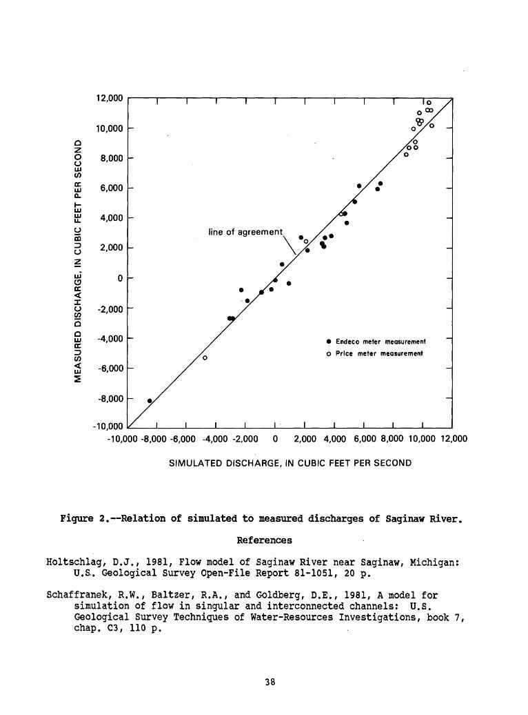
Flow model of Saginaw River near Saginaw, Michigan, by David J. Holtschlag .......................................... 35

Computation of flow and detection of the salt-front location for the Atlantic Intracoastal Waterway in the vicinity of Myrtle Beach, South Carolina, by Curtis L. Sanders ..................... 39

111

PageFlow and transport model of the Atlantic Intracoastal Waterway in

the Grand Strand Area, South Carolina, by Robert E. Schuck-Kolben ...................................... 42

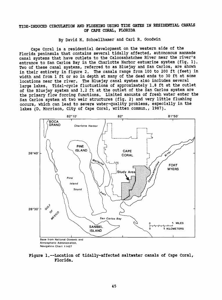
Tide-induced circulation and flushing using tide gates in residential canals of Cape Coral, Florida, by David H. Schoellhamer and Carl R. Goodwin .................... 45

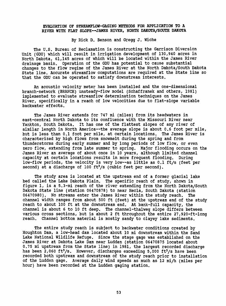
Evaluation of streamflow-gaging methods for application to a river with flat slope James River, North Dakota/South Dakota, by Rick D. Benson and Gregg J. Wiche ............................ 53

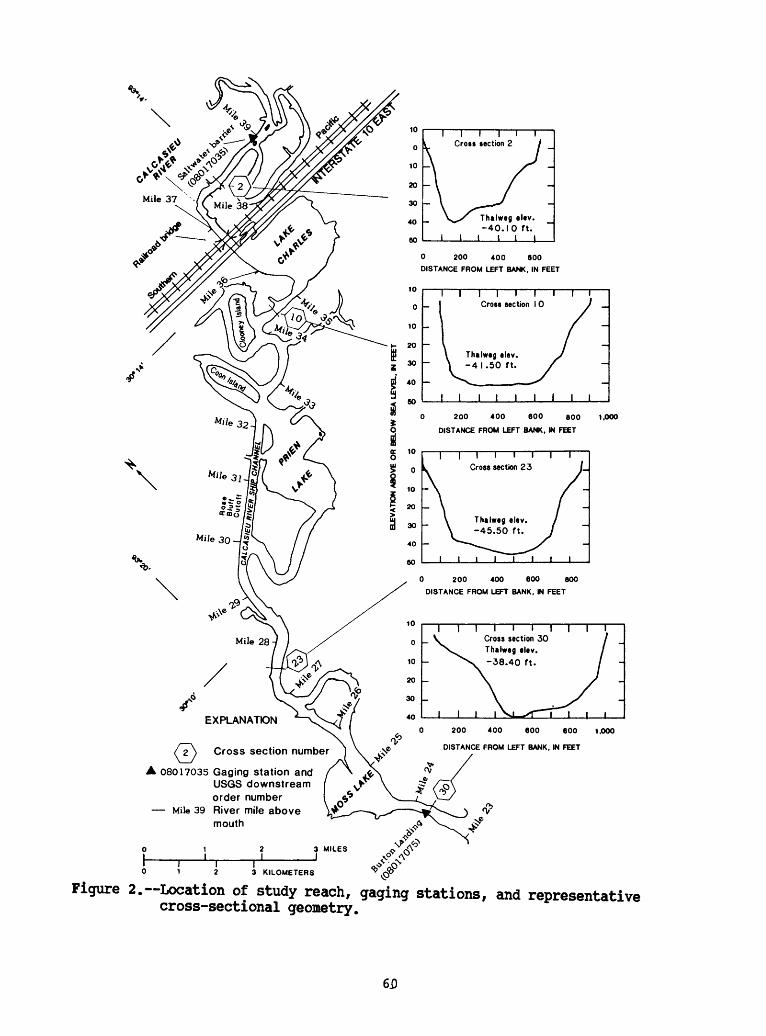
Simulation of flow in the lower Calcasieu River near Lake Charles, Louisiana, by George J. Arcement, Jr. ........................... 58

BRANCH flow model of the Knik and Matanuska Rivers, Alaska, by Stephen W. Lipscomb .......................................... 62

Flow determination for Ohio River at Greenup Dam and Louisville, Kentucky, by Kevin J. Ruhl ...................................... 65

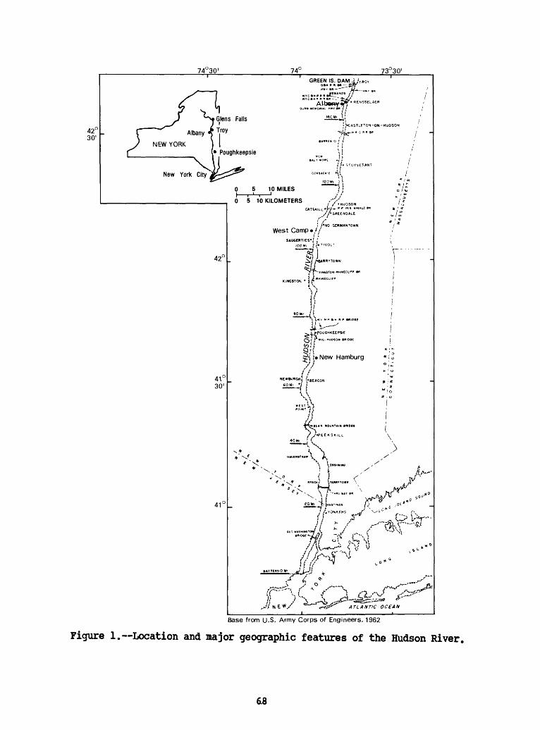
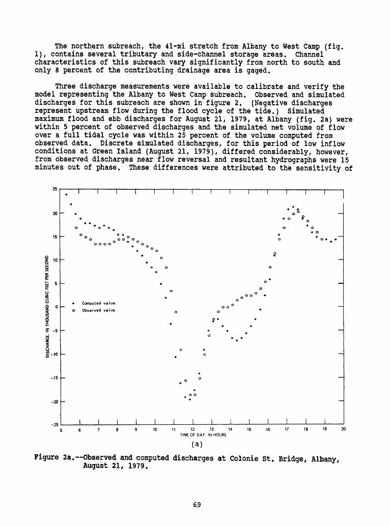
Flow model of the Hudson River from Albany to New Hamburg,New York, by David A. Stedfast .................................. 67

Simulation of debris flows using the HYDRAUX model, by R. Peder Hansen .............................................. 74

Appendix I: Glossary of technical terminology .......................... 77

List of participants ................................................... 99

iv

CONVERSION FACTORS AND ABBREVIATIONS

For readers who prefer metric (International System) units rather than the inch-pound terms used in this report, the following conversion factors may be used:

Multiply inch-pound units

inch (in.)feet (ft)mile (mi)

square inch (in2 )square foot (ft2 )square mile (mi2 )

cubic inch (in3 ) cubic foot (ft3 ) acre-foot (acre-ft)

By

Length

2.540.30481.609

Area

6.4529.294 x 10"2 2.590

Volume

1.639 x 1012.832 x 10"21.233 x 10s

To obtain SI units

centimeter (cm) meter (m) kilometer (km)

square centimeter (cm2 ) square meter (m2 ) square kilometer (km2 )

cubic centimeter (cm3 ) cubic meter (m3 ) cubic meter (m3 )

cubic foot per second(ft3/s)

gallon per minute(gal/min)

Volume per unit time

2.832 x 10-2

6.309 x 10s

Mass per unit volume

cubic meter per second(m3/s)

cubic meter per second(ms/s)

pound per cubic foot(lb/ft3 )

pound per cubic foot

1.602

1.602 x 104

kilogram per cubic meter

gram per cubic centimeter (g/cm3 )

Temperature

degree Celsius = (degree Fahrenheit - 32)/1.8

Sea Level; In this report "sea level" refers to the National Geodetic Vertical Datum of 1929 (NGVD of 1929) a geodetic datum derived from a general adjustment of the first-order level nets of both the United States and Canada, formerly called "Sea Level Datum of 1929".

PROCEEDINGS OF THE ADVANCED SEMINAR ON ONE-DIMENSIONAL, OPEN-CHANNELFLOW AND TRANSPORT MODELING

Compiled by Raymond W. Schaffranek

ABSTRACT

In view of the increased use of mathematical/numerical simulation models, of the diversity of both model investigations and informational project objectives, and of the technical demands of complex model applications by U.S. Geological Survey personnel, an advanced seminar on one-dimensional open-channel flow and transport modeling was organized and held on June 15-18, 1987, at the National Space Technology Laboratory, Bay St. Louis, Mississippi. Principal emphasis in the Seminar was on one-dimensional flow and transport model-implementation techniques, operational practices, and application considerations. The purposes of the Seminar were to provide a forum for the exchange of information, knowledge, and experience among model users, as well as to identify immediate and future needs with respect to model development and enhancement, user support, training requirements, and technology transfer. The Seminar program consisted of a mix of topical and project presentations by Geological Survey personnel. This report is a compilation of short papers that summarize the presentations made at the Seminar.

INTRODUCTION

The processes of numerical model implementation and simulation entail a number of intuitive judgements, critical decisions, and required actions on the part of the modeler. The formal tool of the modeler is a numerical procedure that enables approximate mathematical solutions of the laws governing the particular process being simulated to be obtained. It is encumbent on the modeler to identify and select the most appropriate numerical method and computer model that will yield the best approximate solution of the governing equations without introducing spurious effects. The numerical procedure by which the solution is obtained must be properly and precisely adapted to account for the dominant features of the simulated process. Once the appropriate numerical device is identified, the modeler conducts its implementation by strategically schematizing the waterbody geometry, assigning boundary conditions at internal channel junctions and channel extremities, defining all pertinent forcing functions, and conducting a thorough, precise, calibration and verification effort using field-collected data. It is also encumbent on the modeler to demonstrate how accurately the selected model simulates reality by accounting for the fundamental physical and hydraulic features of the waterbody being simulated. Modeling is, in essence, an art by virtue of the fact that it is premised on the processes of abstraction and replication. It is the responsibility of the modeler, as an artist, to identify the important features that need to be represented and then to ensure that these aspects of the waterbody are properly reflected and considered in the model implementation.

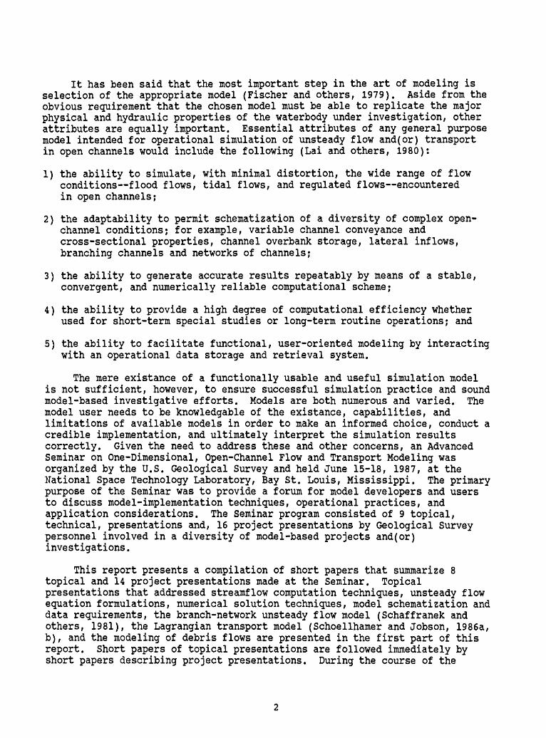
It has been said that the most important step in the art of modeling is selection of the appropriate model (Fischer and others, 1979). Aside from the obvious requirement that the chosen model must be able to replicate the major physical and hydraulic properties of the waterbody under investigation, other attributes are equally important. Essential attributes of any general purpose model intended for operational simulation of unsteady flow and(or) transport in open channels would include the following (Lai and others, 1980):

1) the ability to simulate, with minimal distortion, the wide range of flow conditions flood flows, tidal flows, and regulated flows encountered in open channels;

2) the adaptability to permit schematization of a diversity of complex open- channel conditions; for example, variable channel conveyance and cross-sectional properties, channel overbank storage, lateral inflows, branching channels and networks of channels;

3) the ability to generate accurate results repeatably by means of a stable, convergent, and numerically reliable computational scheme;

4) the ability to provide a high degree of computational efficiency whether used for short-term special studies or long-term routine operations; and

5) the ability to facilitate functional, user-oriented modeling by interacting with an operational data storage and retrieval system.

The mere existance of a functionally usable and useful simulation model is not sufficient, however, to ensure successful simulation practice and sound model-based investigative efforts. Models are both numerous and varied. The model user needs to be knowledgable of the existance, capabilities, and limitations of available models in order to make an informed choice, conduct a credible implementation, and ultimately interpret the simulation results correctly. Given the need to address these and other concerns, an Advanced Seminar on One-Dimensional, Open-Channel Flow and Transport Modeling was organized by the U.S. Geological Survey and held June 15-18, 1987, at the National Space Technology Laboratory, Bay St. Louis, Mississippi. The primary purpose of the Seminar was to provide a forum for model developers and users to discuss model-implementation techniques, operational practices, and application considerations. The Seminar program consisted of 9 topical, technical, presentations and, 16 project presentations by Geological Survey personnel involved in a diversity of model-based projects and(or) investigations.

This report presents a compilation of short papers that summarize 8 topical and 14 project presentations made at the Seminar. Topical presentations that addressed streamflow computation techniques, unsteady flow equation formulations, numerical solution techniques, model schematization and data requirements, the branch-network unsteady flow model (Schaffranek and others, 1981), the Lagrangian transport model (Schoellhamer and Jobson, I986a, b), and the modeling of debris flows are presented in the first part of this report. Short papers of topical presentations are followed immediately by short papers describing project presentations. During the course of the

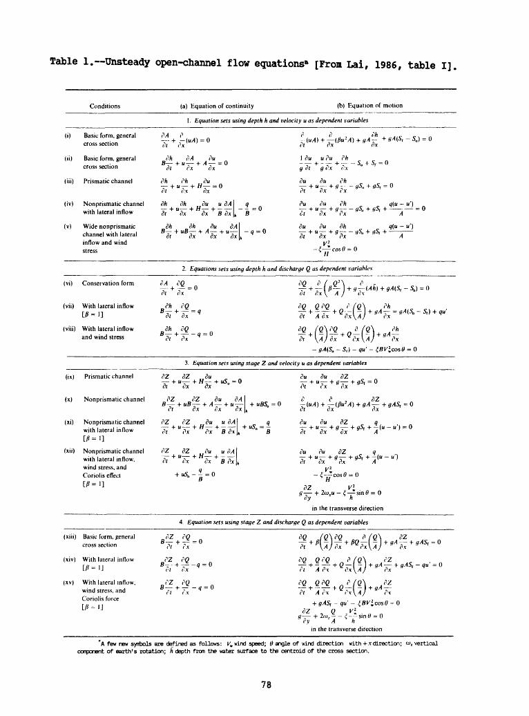
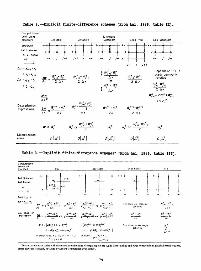
Seminar, topical and project presentations were intermixed to facilitate and(or) stimulate discussion and exchange of ideas. Short papers of project presentations are followed by Appendix I which includes three tables reproduced from Lai (1986) and used extensively throughout the Seminar. Table 1 is a compilation of various formulations of the unsteady open-channel flow equations, Table 2 presents typical explicit finite-difference structures, and Table 3 illustrates a number of implicit finite-difference schemes. Appendix I also includes a glossary of technical terminology, common to the field of computational hydraulics, that was initially, partly, prepared for use at the Seminar and subsequently extended to include additional technical terms identified during the course of the Seminar. At the end of this report is a list of participants at the Seminar.

References

Fischer, H.B., List, E.J., Koh, R.C.Y., Imberger, J., and Brooks, N.H., 1979, Mixing in inland and coastal waters: New York, New York, Academic Press, 483 p.

Lai, Chintu, 1986, Numerical modeling of unsteady open-channel flow, in Advances in Hydroscience: Chow, V.T., and Yen, B.C., eds., Academic Press, Orlando, Florida, v. 14, p. 161-333.

Lai, Chintu, Baltzer, R.A., and Schaffranek, R.W., 1980, Techniques and Experiences in the utilization of unsteady open-channel flow models: American Society of civil Engineers, Specialty Conference on Computer and Physical Modeling in Hydraulic Engineering, Chicago, Illinois, August 6-8, 1980, Proceedings, p. 177-191.

Schaffranek, R.W., Baltzer, R.A., and Goldberg, D.E., 1981, A model for simulation of flow in singular and interconnected channels: U.S. Geological Survey Techniques of Water-Resources Investigations, book 7, chap. C3, 110 p.

Schoellhamer, D.H., and Jobson, H.E., 1986a, Programmers manual for a one- dimensional Lagrangian transport model: U.S. Geological Survey Water- Resources Investigations Report 86-4144, 101 p.

1986b, Users manual for a one-dimensional Lagrangian transport model U.S. Geological Survey Water-Resources Investigations Report 86-4145, 95 p.

CONTRASTING ONE-DIMENSIONAL, UNSTEADY FLOW MODELS TO TRADITIONAL METHODS OF FLOW ROUTING AND STREAMFLOW COMPUTATION

By Vernon B. Sauer

Varied methods exist for computing flow in open-channel reaches. The nature of the flow conditions and(or) data limitations resulting from field constraints typically dictate the method of use. Nevertheless, careful critical review of available methods is a practical first step in flow routing and streamflow computation.

Traditional flow-routing and streamflow-computation techniques, such as step-backwater for computing water surface profiles (Davidian, 1984, Shearman, 1976, Shearman and others, 1986) and stage-discharge relations for computing unit and daily discharges (Rantz and others, 1982), are steady-flow methods that are sometimes used to simulate unsteady conditions. These techniques will not, however, account for changing backwater and hysteresis effects. Attempts to incorporate other properties, such as measured fall, velocity, or rate-of-change in stage, can improve discharge ratings so that variable backwater or hysteresis effects can somewhat be accounted for, but these approaches are not always entirely satisfactory. A two-section, Manning equation method that would account for backwater and hysteresis effects has been proposed by Rantz and others (1982) to improve backwater ratings, but it is presently untested. A one-section, unsteady flow-computation technique to account for hysteresis but not variable backwater effects has been tested by Faye and Blalock (1984) and may be applicable in some situations if adequate calibration can be accomplished. Flow-routing models based on convolution methods (Doyle and others, 1983), Muskingum, or regression techniques are generally easy to use, but likewise do not adequately account for changing backwater and hysteresis effects.

Routing by one-dimensional solution of the unsteady-flow equations, such as in the branch-network (BRANCH) unsteady-flow model (Schaffranek and others, 1981), is used extensively in the Southeastern United States for both project activities and routine computation of streamflow records (Schaffranek, 1987) by U.S. Geological Survey personnel. One-dimensional, unsteady flow-routing models have proven to be a superior method in most situations where severe backwater and(or) hysteresis conditions are evident. Although unsteady flow models may not be best, or even necessary, in all studies they should be considered as viable computation techniques. They are acceptable for computing basic streamflow records and generally are superior to stage-fall-discharge, rate-of-change-in-stage, and some velocity-index ratings. An additional advantage of unsteady flow models is their capability to compute continuous conditions throughout river reaches and open-channel networks.

References

Davidian, Jacob, 1984, Computation of water-surface profiles: U.S.Geological Survey Techniques of Water-Resources Investigations, book 3, chap. A15, 48 p.

Doyle, W.H., Jr., Shearman, J.O., Stiltner, G.J., and Krug, W.R., 1983, A digital model for streamflow routing by convolution methods: U.S. Geological Survey Water-Resources Investigations Report 83-4160, 130 p.

Faye, R.E., and Blalock, M.E., 1984, Simulation of dynamic flood flows atgaged stations in the southeastern United States: U.S. Geological Survey Water-Resources Investigations Report 84-4, 114 p.

Rantz, S.E., and others, 1982, Measurement and computation of streamflow:Volume 2. Computation of discharge: U.S. Geological Survey Water-Supply Paper 2175, 631 p.

Schaffranek, R.W., 1987, Flow model for open-channel reach or network: U.S. Geological Survey Professional Paper 1384, 11 p.


Shearman, J.O., 1976, Computer applications for step-backwater and floodway analysis: U.S. Geological Survey Open-File Report 76-449, 103 p.

Shearman, J.O., Kirby, W.H., Schneider, V.R., and Flippo, H.N., 1986, Bridge waterways analysis model: research report: U.S. Department of Transportation, Federal Highway Administration Report No. FHWA/RD-86/108, 112 p.

THE ONE-DIMENSIONAL EQUATIONS OF UNSTEADY OPEN-CHANNEL FLOW

By Jonathan K. Lee

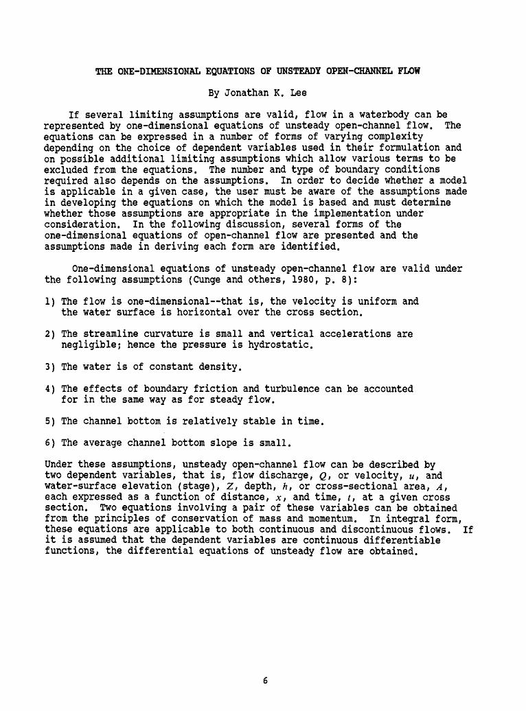
If several limiting assumptions are valid, flow in a waterbody can be represented by one-dimensional equations of unsteady open-channel flow. The equations can be expressed in a number of forms of varying complexity depending on the choice of dependent variables used in their formulation and on possible additional limiting assumptions which allow various terms to be excluded from the equations. The number and type of boundary conditions required also depends on the assumptions. In order to decide whether a model is applicable in a given case, the user must be aware of the assumptions made in developing the equations on which the model is based and must determine whether those assumptions are appropriate in the implementation under consideration. In the following discussion, several forms of the one-dimensional equations of open-channel flow are presented and the assumptions made in deriving each form are identified.

One-dimensional equations of unsteady open-channel flow are valid under the following assumptions (Cunge and others, 1980, p. 8):

1) The flow is one-dimensional that is, the velocity is uniform and the water surface is horizontal over the cross section.

2) The streamline curvature is small and vertical accelerations are negligible; hence the pressure is hydrostatic.

3) The water is of constant density.

4) The effects of boundary friction and turbulence can be accounted for in the same way as for steady flow.

5) The channel bottom is relatively stable in time.

6) The average channel bottom slope is small.

Under these assumptions, unsteady open-channel flow can be described by two dependent variables, that is, flow discharge, Q, or velocity, u, and water-surface elevation (stage), Z, depth, h, or cross-sectional area, A, each expressed as a function of distance, x, and time, /, at a given cross section. Two equations involving a pair of these variables can be obtained from the principles of conservation of mass and momentum. In integral form, these equations are applicable to both continuous and discontinuous flows. If it is assumed that the dependent variables are continuous differentiable functions, the differential equations of unsteady flow are obtained.

The continuity equation, or the equation for conservation of mass, can be written

^ + 22-«,dt dx q

or

[1] [2] [3] [4] [5]

dh , dA , du ^ dhB + u I + A + uB = q, 2

dt dx*h dx dx

where q is the lateral inflow and B is the top width (Lai, 1986, p. 180).

The dynamic equation can be written

dO d f -^ rdh ^f + £ («2) + gA (~ - S0 ]+ gAS, = ««', (3)

or

[6] [7] [8] [9] [10] [11]

*« + '-". + *s --<«-« >.where # is acceleration due to gravity, S0 is the bed slope, 5f is the friction slope, and u l is the x-component of velocity associated with the lateral inflow, q.

Equations 2 and 4 constitute a typical form of the equations of unsteady gradually varied flow. These equations are frequently referred to as the Saint-Venant equations, the one-dimensional unsteady shallow-water equations, the unsteady nearly horizontal flow equations, the unsteady open-channel flow equations, or other variations thereof.

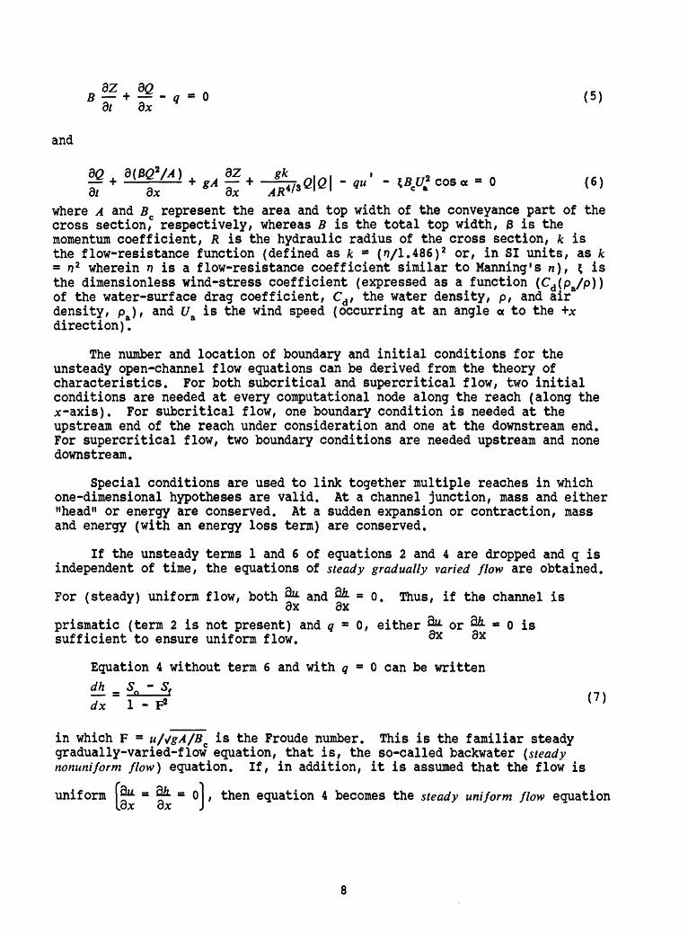
The unsteady open-channel flow equations can be written in terms of a number of possible combinations of dependent variables, that is, h-u, h-Q, Z-u, or Z-Q , and additional terms can be added to account for wind, Coriolis, and other effects as necessary. Table 1 in Appendix I (modified from Lai, 1986, p. 182, 183, Table I) lists a number of possible equation sets and some of their variations. The equation set for the U.S. Geological Survey operational branch-network (BRANCH) unsteady-flow model (Schaffranek, 1987) is formulated to account for overbank storage, nonuniform velocity distribution, and wind stress effects. The BRANCH model equations, using stage, Z, and discharge, Q, as dependent variables, are expressed as

?*£- and

where A and Bc represent the area and top width of the conveyance part of the cross section,0 respectively, whereas B is the total top width, 0 is the momentum coefficient, R is the hydraulic radius of the cross section, k is the flow-resistance function (defined as k - (n/lAB6) 2 or, in SI units, as k >7 2 wherein n is a flow-resistance coefficient similar to Manning's «), $ is the dimensionless wind-stress coefficient (expressed as a function (Cd (pa/p)) of the water-surface drag coefficient, Cd , the water density, p, and air density, pa ), and U& is the wind speed (occurring at an angle a to the +x direction)*

The number and location of boundary and initial conditions for the unsteady open-channel flow equations can be derived from the theory of characteristics. For both subcritical and supercritical flow, two initial conditions are needed at every computational node along the reach (along the x-axis). For subcritical flow, one boundary condition is needed at the upstream end of the reach under consideration and one at the downstream end. For supercritical flow, two boundary conditions are needed upstream and none downstream.

Special conditions are used to link together multiple reaches in which one-dimensional hypotheses are valid. At a channel junction, mass and either "head" or energy are conserved. At a sudden expansion or contraction, mass and energy (with an energy loss term) are conserved.

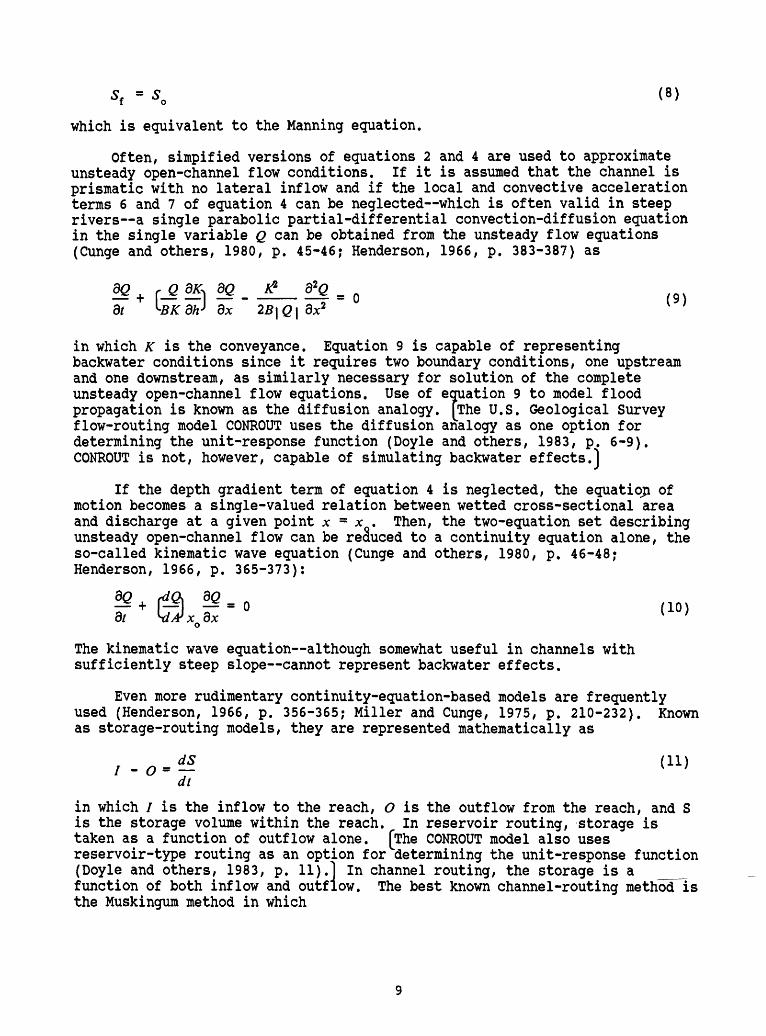
If the unsteady terms 1 and 6 of equations 2 and 4 are dropped and q is independent of time, the equations of steady gradually varied flow are obtained.

For (steady) uniform flow, both &* and 2t = o. Thus, if the channel is3x ax

prismatic (term 2 is not present) and q * 0, either ^M. or ^fi. o is sufficient to ensure uniform flow. 9x 9x

Equation 4 without term 6 and with q - 0 can be written dh _ Sn - Sf

in which F = u/vgA/Bc is the Froude number. This is the familiar steady gradually-varied-flow equation, that is, the so-called backwater (steady nonuniform flow) equation. If, in addition, it is assumed that the flow is

uniform 5"- a <& a 0 L then equation 4 becomes the steady uniform flow equation (.ox ox j

S, = S0 (8)

which is equivalent to the Manning equation.

Often, simpified versions of equations 2 and 4 are used to approximate unsteady open-channel flow conditions. If it is assumed that the channel is prismatic with no lateral inflow and if the local and convective acceleration terms 6 and 7 of equation 4 can be neglected which is often valid in steep rivers a single parabolic partial-differential convection-diffusion equation in the single variable Q can be obtained from the unsteady flow equations (Cunge and others, 1980, p. 45-46; Henderson, 1966, p. 383-387) as

dx 2B\Q\

in which K is the conveyance. Equation 9 is capable of representing backwater conditions since it requires two boundary conditions, one upstream and one downstream, as similarly necessary for solution of the complete unsteady open-channel flow equations. Use of equation 9 to model flood propagation is known as the diffusion analogy. [The U.S. Geological Survey flow-routing model CONROUT uses the diffusion analogy as one option for determining the unit-response function (Doyle and others, 1983, p. 6-9). CONROUT is not, however, capable of simulating backwater effects.]

If the depth gradient term of equation 4 is neglected, the equatioji of motion becomes a single-valued relation between wetted cross-sectional area and discharge at a given point x = x . Then, the two-equation set describing unsteady open-channel flow can be reduced to a continuity equation alone, the so-called kinematic wave equation (Cunge and others, 1980, p. 46-48; Henderson, 1966, p. 365-373):

The kinematic wave equation although somewhat useful in channels with sufficiently steep slope cannot represent backwater effects.

Even more rudimentary continuity-equation-based models are frequently used (Henderson, 1966, p. 356-365; Miller and Cunge, 1975, p. 210-232). Known as storage -rout ing models, they are represented mathematically as

dt

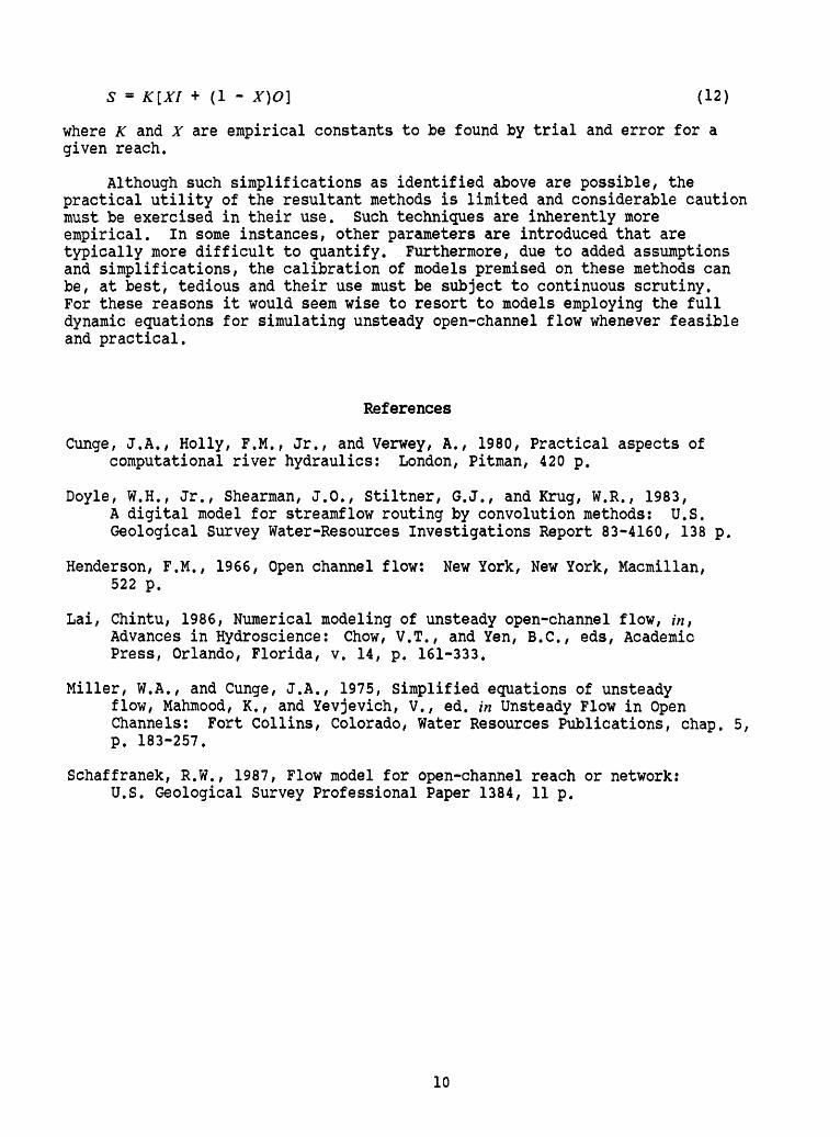
in which / is the inflow to the reach, O is the outflow from the reach, and S is the storage volume within the reach. In reservoir routing, storage is taken as a function of outflow alone. [The CONROUT model also uses reservoir-type routing as an option for determining the unit-response function (Doyle and others, 1983, p. 11).] In channel routing, the storage is a function of both inflow and outflow. The best known channel -rout ing methodTis the Muskingum method in which

S - K[XI + (1

where /: and X are empirical constants to be found by trial and error for a given reach.

Although such simplifications as identified above are possible, the practical utility of the resultant methods is limited and considerable caution must be exercised in their use. Such techniques are inherently more empirical. In some instances, other parameters are introduced that are typically more difficult to quantify. Furthermore, due to added assumptions and simplifications, the calibration of models premised on these methods can be, at best, tedious and their use must be subject to continuous scrutiny. For these reasons it would seem wise to resort to models employing the full dynamic equations for simulating unsteady open-channel flow whenever feasible and practical.

References

Cunge, J.A., Holly, F.M., Jr., and Verwey, A., 1980, Practical aspects of computational river hydraulics: London, Pitman, 420 p.

Doyle, W.H., Jr., Shearman, J.O., Stiltner, G.J., and Krug, W.R., 1983, A digital model for streamflow routing by convolution methods: U.S. Geological Survey Water-Resources Investigations Report 83-4160, 138 p.

Henderson, F.M., 1966, Open channel flow: New York, New York, Macmillan, 522 p.

Lai, Chintu, 1986, Numerical modeling of unsteady open-channel flow, in, Advances in Hydroscience: Chow, V.T., and Yen, B.C., eds, Academic Press, Orlando, Florida, v. 14, p. 161-333.

Miller, W.A., and Cunge, J.A., 1975, Simplified equations of unsteady flow, Mahmood, K., and Yevjevich, V., ed. in Unsteady Flow in Open Channels: Fort Collins, Colorado, Water Resources Publications, chap. 5, p. 183-257.

Schaffranek, R.W., 1987, Flow model for open-channel reach or network: U.S. Geological Survey Professional Paper 1384, 11 p.

10

CHARACTERISTICS OF COMMON NUMERICAL SOLUTIONS AND THEIR OPERATIONAL RAMIFICATIONS

By Ralph T. Cheng

Numerical solutions for unsteady open-channel flows are discrete approximations to the analytical solutions of the governing equations (Chow, 1959). Depending on the nature of the applications, the governing St. Venant shallow-water equations can be written in a variety of forms (Lai, 1986). These governing equations can be discretized by means of finite-difference methods (Cunge and others, 1980; Fread, 1974; Lai, 1986; Liggett and Cunge, 1975), finite-element methods (Smith and Cheng, 1976), or methods of characteristics (Abbott, 1976; Abbott, 1979; Goldberg and Wylie, 1983; Liggett and Cunge, 1975).

In the time domain, methods of solution can be classified as explicit or implicit (Lai, 1986; Liggett and Cunge, 1975). Explicit numerical methods invoke solution of the dependent variables on the future time level one grid point at a time, independent from all other unknowns on the future time level. Implicit methods solve for all dependent variables in a coupled discrete system. Commonly used explicit and implicit finite-difference algorithms are given in tables 2 and 3 in Appendix I (modified from Lai, 1986, p. 218, 223, Table II, Table III). The fixed-grid method of characteristics is actually a method based on a combined Eulerian and Lagrangian formulation (Abbott, 1979; Cheng, 1983; Cheng and others, 1984; Holly and Preissmann, 1977; Sivaloganathan, 1979). Its formulation can be given in both explicit (Casulli and others, 1985) and implicit forms (Schmitz and Edenhofer, 1983).

"Every proposed (numerical) scheme should be submitted to convergence analysis 11 (Cunge and others, 1980). For linear governing equations, convergence can be ensured if the following conditions, known as Lax's equivalence theorem, are satisfied (Cunge and others, 1980): "Given a properly posed initial-value problem and a finite-difference approximation to it that satisfies the consistency condition, stability is the necessary and sufficient condition for convergence". Here consistency implies, roughly, that the discrete operators approach the differential equations as the discrete elements tend to zero. Thus, in numerical modeling studies, one must insure: (1) the discrete methods of solution satisfy the consistency condition, and (2) the numerical methods are stable. Satisfaction of these two conditions implies that the numerical solutions are assured to converge to the analytical solutions of the differential equations.

Because the governing equations for unsteady open-channel flow cover a large variety of conditions (Abbott, 1976; Cunge and others, 1980; Sobey, 1984), there is not one single method of solution, or one particular model, that can solve all flow problems. For a successful modeling study, the following considerations are recommended (Cheng, 1986): (1) ascertain a complete understanding of the nature of the physical problem and (2) choose a valid and effective numerical method or model for solution of the problem.

11

References

Abbott, M.B., 1976, Computational hydraulics, a short pathology: Journal of Hydrologic Research, v. 14, no. 4, p. 421-447.

Abbott, M.B., 1979, Computational hydraulics, elements of theory of free surface flows: London, Pitman, 324 p.

Casulli, V., Pontrelli, G., and Secchi, P., 1985, An Eulerian-Lagrangianmethod for open channel flows: 4th International Conference in Numerical Methods of Laminar and Turbulent Flows, Swansea, U.K., Pineridge Press, Proceedings, p. 1360-1370.

Cheng, R.T., 1983, Euler-Lagrangian computations in estuarine hydrodynamics: C. Taylor and others, eds., 3rd International Conference in Numerical Methods of Laminar and Turbulent Flows, Swansea, U.K., Pineridge Press, Proceedings, p. 341-352.

Cheng, R.T., Casulli, V., and Milford, S.N., 1984, Eulerian-Lagrangiansolution of convection-dispersion equation in natural coordinates: Water Resources Research, v. 20, no. 7, p. 944-952.

Cheng, R.T., 1986, Modeling of estuarine hydrodynamics a mixture of art and science: Third International Symposium on River Sedimentation, University of Mississippi, Proceedings, p. 1468-1475.

Chow, V.T., 1959, Open channel hydraulics: New York, New York, McGraw-Hill, 680 p.

Cunge, J.A., Holly, Jr., F.M., and Verwey, A., 1980, Practical aspects of computational river hydraulics: chap. 3, Solution Techniques and Their Evaluation, London, Pitman, p. 53-146.

Fread, D.L., 1974, Numerical properties of implicit four-point finite- difference equations of unsteady flow: NOAA Technical Memorandum, NWS, HYDRO-18, 38 p.

Goldberg, D.E., and Wylie, E.B., 1983, Characteristics method using time-line interpolations: American Society of Civil Engineers, Journal of the Hydraulics Division, v. 105, no. HY5, p. 670-683.

Holly, F.M., Jr., and Preissmann, A., 1977, Accurate calculation of transport in two dimensions: American Society of Civil Engineers, Journal of the Hydraulics Division, v. 103, no. HY11, p. 1259-1428.

Lai, Chintu, 1986, Numerical modeling of unsteady open-channel flow, in Advances in Hydroscience: Chow, V.T., and Yen, B.C., eds., Academic Press, Orlando, Florida, v. 14, p. 161-333.

Liggett, J.A., and Cunge, J.A., 1975, Numerical methods of solution ofthe unsteady flow equations, Mahmood, K., and Yevjevich, V., eds., in Unsteady Flow in Open Channels: Fort Collins, Colorado, Water Resources Publications, chap. 4, p. 89-179.

12

Schmitz, G., and Edenhofer, J., 1983, Flood routing in the Danube River by the new implicit method of characteristics (IMOC): 3rd International.. Conference on Applied Mathematical Modeling, Mitteilungen des Inst. fur Meereskunde der 3rd Univ., Hamburg, West Germany, Proceedings, 13 p.

Sivaloganathan, K., 1979, Channel flow computations using characteristics: American Society of Civil Engineers, Journal of the Hydraulics Division, v. 105, no. HY7, p. 899-910.

Smith, L.H., and Cheng, R.T., 1976, A gelerkin finite element solution of the one-dimensional unsteady flow problems using a cubic hermite polynomial basis function: American Society of Civil Engineers, 15th International Conference on Coastal Engineering, Honolulu, Hawaii, Proceedings, p. 3358-3376.

Sobey, R.J., 1984, Numerical alternatives in transient stream response:American Society of Civil Engineers, Journal of the Hydraulics Division, v. 110, no. 6, p. 749-772.

13

EVOLUTION AND OPERATIONAL STATUS OF THE BRANCH-NETWORK UNSTEADY FLOW MODEL

By Raymond W. Schaffranek

The branch-network (BRANCH) unsteady-flow model was originally formulated, developed, and tested during the 1976-1980 time period within the National Research Program of the Water Resources Division (WRD) of the U.S. Geological Survey. The general purpose flow-simulation model was subsequently documented for operational use in 1981 by the program developers. (See Schaffranek and others, 1981.) The model was officially announced for operational use within WRD in 1981 via Surface Water Branch Technical Memorandum 82.03, which accompanied distribution of the model documentation. Subsequent to its original development and documentation, the model has undergone a number of revisions as new features and capabilities have been incorporated.

The model is as a more powerful and versatile computational alternative to stage-fall and other slope-type rating techniques. It has been demonstrated to be particularly appropriate and cost effective for assessing flows in regulated rivers and in rivers where backwater conditions are prevalent. As is illustrated in the original documentation, as well as in subsequent reports (Schaffranek, 1985a,b, 1987a,b), the model is well suited for simulation of regulated, tidal, or meteorological-driven flows in such diverse upland or coastal open-channel configurations as singular river reaches; rivers comprised of contiguous multiple reaches; or networks of channels connected in sequential order, in a dendritic arrangement, or in a looped pattern.

Subsequent to the original development and documentation of BRANCH, numerous enhancements, extensions, and revisions have been made. In summary, the present operational version of BRANCH has the following basic attributes and capabilities:

numerically solves a complete set of the one-dimensional, unsteady, open-channel flow equations including nodal and lateral flows, overbank storage, nonuniform velocity distributions, and wind-stress effects,

uses an adjustable, weighted, four-point, implicit finite-difference scheme,

employs a nonlinear, iterative matrix-solution method with user-specified tolerance controls,

is equally applicable to a single reach (branch) of channel defined by a single channel segment or contiguous multiple segments, and, to multiple branches connected in sequence, in a dendritic layout, or in a looped (network) configuration,

uses observed, estimated, or previously computed initial conditions,

uses historical, real-time, or hypothetical water-level or discharge boundary conditions,

14

uses cross-sectional geometry defined by piece-wise, linear relations,

employs user-selectable constant, functional, or tabular frictional resistance (energy loss),

interacts with an operational, time-dependent, input/output data base system,

uses English or metric units for input/output,

offers numerous output data types in a variety of formats,

generates a variety of digital plots on widely used digital-graphic devices,

produces flow conditions for Lagrangian transport model,

offers user-friendly, interactive model setup and input/output file designation,

is coded in standard, transportable Fortran 77,

is executable on mainframe (IBM or Amdahl), minicomputer (Prime), or microcomputer (IBM/PC or compatible) systems,

is documented in U.S. Geological Survey publications, thoroughly field tested, and widely used for a broad range of field situations and varied flow conditions,

continues to be developed to handle newly identified needs and enhanced to take advantage of advances in computational hydraulics and computer technology.

The model has been compiled, executed, and tested on a variety of computer systems using various Fortran 77 compilers. Evaluation of the model's performance in simulating a network of 25 branches in which flow is computed every 15 minutes at 69 cross sections and the movement of eight index particles representing conservative constituents is tracked, indicates that less than 1 minute (48 seconds) of central processing unit (CPU) time is required to conduct one day of simulation on a Prime 9955 minicomputer system. By contrast, the same simulation on a Zenith 151 XT personal computer, operating at a clock speed of 4.77 MHz (megahertz), requires nearly 1 hour (51 minutes) of CPU time per simulated day. Further comparison with a 32-bit Sun Microsystems 3/160 engineering work-station system, operating at 16.7 MHz clock speed, indicates that simulations would require 5.3 minutes of CPU time per simulated day.

The BRANCH model is currently in operational use at nearly 40 sites as conducted by more than a dozen Geological Survey offices. Studies involving water-withdrawal effects, bridge location analyses, flood inundation, and tide-induced flows are being conducted. BRANCH is now the recognized standard for the simulation of unsteady open-channel flow within the U.S. Geological Survey.

15

References

Schaffranek, R.W., 1985a, Model for simulating floods in rivers:1985 Society for Computer Simulation Multiconference, Computer Simulation in Emergency Planning Session, Jan. 24-26, 1985, Simulation Series v. 15, no. 1, p. 132-139.

Schaffranek, R.W., 1985b, Simulating flow in the tidal Potomac River: American Society of Civil Engineers Hydraulics Division Specialty Conference, Lake Buena Vista, Florida, August 12-17, 1985, Proceedings, v. 1, p. 134-140.

Schaffranek, R.W., 1987a, Flow model for open-channel reach or network: U.S. Geological Survey Professional Paper 1384, 11 p.

Schaffranek, R.W., 1987b, A flow-simulation model of the tidal Potomac River: U.S. Geological Survey Water-Supply Paper 2234-D, 41 p.


16

TREATMENT OF NONHOMOGENEOUS TERMS AND PARAMETERS IN MODEL CALIBRATION AND FLOW SIMULATION

By Chintu Lai

Two important aspects of model implementation are proper consideration and treatment of effects accounted for by nonhomogeneous terms in the fundamental equations and use of appropriate and legitimate model-adjustment procedures. These factors go hand-in-hand for a number of reasons. Comprehensive forms of the fully dynamic, open-channel flow equations contain a variety of nonhomogeneous terms that make the governing differential equations and thus, the flow-simulation models formulated on them more versatile and adaptable to a broader spectrum of real-world, engineering problems (Lai, 1986). Inclusion of these terms, however, tends to complicate the mathematical formulation and development of models and also places greater emphasis on the need for practical guidelines and rational procedures for model users to follow in their implementation and calibration efforts.

Information on the relative significance, effects, and benefits of using models that include the nonhomogeneous terms is in great need. Efforts are now underway within the National Research Program of the Water Resources Division to analyze five particular nonhomogeneous terms, representing bed slope, frictional slope, nonprismatic channel geometry, lateral flow, and wind stress. Three types of flow models are being used in this study. Two of these models are in dimensional form; one using the method of characteristics (HOC) (Lai, 1965; 1967; Lai and Onions, 1976) and the other, called BRANCH, using a four-point, implicit finite-difference method (Schaffranek and others, 1981). The third model, which also uses the method of characteristics is a dimensionless version. By selecting suitable base quantities, a set of flow data from Threemile Slough, near Rio Vista, Calif., for July 15-16, 1959 (Lai, 1965; Baltzer and Lai, 1968) has been normalized and a series of numerical experiments are being conducted using the dimensionless model. Initial findings (Lai and others, 1987) indicate that the numerical experiments will yield practical guides for model calibration, development, and implementation.

Useful information on techniques and procedures for parameter calibration and model adjustment began to surface almost at the inception of numerical modeling and simulation. Fundamental theories and approaches have steadily been advanced and practical experiences and techniques have progressively been enhanced and reported (Baltzer and Lai, 1968; Lai and others, 1978; Davidson and others, 1978, Fread and Smith, 1978). In one particular study (Lai, 1981, 1986), a concise, yet systematic, account of "procedures and techniques for rational model adjustment" has been developed and reported. In this study, three major factors important to precise model calibration that is, water- surface slope, cross-sectional area, and the flow-resistance coefficient were analyzed and evaluated. These factors are clearly demonstrated to be closely correlated to the nonhomogeneous frictional-slope term as well as to some parameters and boundary conditions used to conduct the study. Secondary and special parameters are also enumerated which correspond to other nonhomo geneous terms and related parameters. From the experiences described by Lai (1981), techniques and approaches have been developed and demonstrated to handle these important factors in model calibration and adjustment.

17

References

Baltzer, R.A., and Lai, Chintu, 1968, Computer simulation of unsteady flows in waterways: American Society of Civil Engineers, Journal of the Hydraulics Division, v. 94, no. HY4, p. 1083-1117.

Davidson, B., Vichnevetsky, R., and Wang, H. T., 1978, Numerical techniquesfor estimating best-distributed Manning's roughness coefficients for open estuarial river systems: American Geophysical Union, Water Resources Research, v. 14, no. 5, p. 777-789.

Fread, D.L., and Smith, G.F., 1978, Calibration technique for 1-D unsteady flow models: American Society of Civil Engineers, Journal of the Hydraulics Division, v. 104, no. HY7, p. 1027-1044.

Lai, Chintu, 1965, Flows of homogeneous density in tidal reaches, solution by the method of characteristics: U.S. Geological Survey Open-File Report 65-93, 58 p.

Lai, Chintu, 1967, Computation of transient flows in rivers and estuaries by the multiple-reach method of characteristics: U.S. Geological Survey Professional Paper 575-B, p. B228-B232.

Lai, Chintu, 1981, Procedures and techniques for rational model adjustment in numerical simulation of transient open-channel flow: International Conference on Numerical Modeling in River, Channel Overland Flow of Water Resources Environmental Applications, Bratislava, Czechoslovakia, May 4-8, 1981, Proceedings, 12 p.

Lai, Chintu, 1986, Numerical modeling of unsteady open-channel flow, in Advances in Hydroscience: Chow, V.T., and Yen, B.C.,. eds, Academic Press, Orlando, Florida, v. 14, p. 161-333.

Lai, Chintu, and Onions, C.A., 1976, Computation of unsteady flows in rivers and estuaries by the method of characteristics: (Computer Contribution) U.S. Geological Survey, available from U.S. Department of Commerce, National Technical Information Service, Springfield, Virginia, Report PB-253 785, 195 p.

Lai, Chintu, Schaffranek, R.W., and Baltzer, R.A., 1978, An operational system for implementing simulation models, a case study: American Society of Civil Engineers Specialty Conference on Verification of Mathematical and Physical Models in Hydraulic Engineering, College Park, Maryland, August 9-11, 1978, Proceedings, p. 415-454.

Lai, Chintu, Schaffranek, R.W., and Baltzer, R.A., 1987, Nonhomogeneous terms in the unsteady flow equations: modeling aspects: American Society of Civil Engineers National Conference on Hydraulic Engineering, Williamsburg, Virginia, August 3-7, 1987, Proceedings, p. 351-358.


18

CONCEPTS, EQUATIONS, AND BOUNDARY CONDITIONS OF ONE-DIMENSIONAL TRANSPORT MODELING

By Harvey E. Jobson

The one-dimensional branched Lagrangian transport model (BLTM) simulates the transport and reaction kinetics of up to ten water-quality constituents in fixed channels with known unidirectional or bidirectional flows (Jobson and Schoellhamer, 1987). Data required by the BLTM includes river and inflow discharges, areas, and top widths at cross sections along the study reach, dispersion information such as acquired from a dye injection study, and constituent concentrations at inflow boundaries. Hydraulic and concentration data for the BLTM can be retrieved from the Time-Dependent Data Base (TDDB) of the Time-Dependent Data System (TDDS) (Lai and others, 1978) utilized by the BRANCH model (Schaffranek and others, 1981) to store computed flow information or from formatted sequential-access files. Reaction kinetics are supplied by the user just as in the single-reach LTM version (Schoellhamer and Jobson, 1986a,b), but a subroutine which mimics the QUAL-II kinetics is available. Flow hydraulics can also be supplied by a simplified routing scheme based on the diffusion analogy and subroutines are available to input complete data sets to run the model interactively.

References

Jobson, H.E., and Schoellhamer, D.H., 1987, Users manual for a branched Lagrangian transport model: U.S. Geological Survey Water-Resources Investigations Report, 87-4163, 73 p.

Lai, Chintu, Schaffranek, R.W., and Baltzer, R.A., 1978, An operational system for implementing simulation models, a case study: American Society of Civil Engineers Specialty Conference on Verification of Mathematical and Physical Models in Hydraulic Engineering, College Park, Maryland, August 9-11, 1978, Proceedings, p. 415-454.


Schoellhamer, D.H., and Jobson, H.E., I986a, Programmers manual for a one- dimensional Lagrangian transport model: U.S. Geological Survey Water- Resources Investigations Report 86-4144, 101 p.

1986b, Users manual for a one-dimensional Lagrangian transport model: U.S. Geological Survey Water-Resources Investigations Report 86-4145, 95 P.

19

IMPLEMENTATION OF THE LAGRANGIAN TRANSPORT MODEL

By David H. Schoellhamer

The one-dimensional Lagrangian Transport Model (LTM) simulates the transport and reaction kinetics of up to ten water-quality constituents in fixed channels with known steady or unsteady unidirectional flows (Schoellhamer and Jobson, 1986a, b). The data required by the LTM includes river and inflow discharges, areas, and top widths at cross sections along the study reach, dispersion information such as acquired from a dye injection study, and constituent concentrations at inflow boundaries. The hydraulic and concentration data for the LTM can be retrieved from the Time-Dependent Data Base (TDDB) of the Time-Dependent Data System (TDDS) (Lai and others, 1978) utilized by the BRANCH model (Schaffranek and others, 1981) to store computed flow information. The LTM application steps are (1) determine the flow field, (2) calibrate dispersion, (3) calibrate reaction rate coefficients, and (4) verify the model. The reaction kinetics are supplied by the user in a decay coefficient subroutine so the user has great flexibility to define the interaction of constituents. Examples of LTM applications include suspended-sediment transport in the Mississippi River (Schoellhamer and Curwick, 1986) and in a laboratory flume (Schoellhamer, 1987) and water-quality modeling of the Chattahoochee River (Jobson, 1984, 1987) including the QUAL-II reaction kinetics (Schoellhamer, in press). A similar Branched Lagrangian Transport Model (BLTM) for simulating transport in networks of channels with unsteady bidirectional flow (Jobson and Schoellhamer, 1987) has been applied to a canal system in Cape Coral, Florida.

References

Jobson, H.E., 1984, Simulating unsteady transport of nitrogen, biochemicaloxygen demand, and dissolved oxygen in the Chattahoochee River downstream from Atlanta, Georgia: U.S. Geological Survey Water-supply Paper 2264, 36 p.

Jobson, H.E., 1987, Lagrangian model of nitrogen kinetics in theChattahoochee River: American Society of Civil Engineers, Journal of Environmental Engineering, v. 113, no. 2, p. 223-242.


Lai, Chintu, Schaffranek, R.W., and Baltzer, R.A., 1978, An operational system for implementing simulation models, a case study: American Society of Civil Engineers Specialty Conference on Verification of Mathematical and Physical Models in Hydraulic Engineering, College Park, Maryland, August 9-11 1978, Proceedings, p. 415-545.


20

Schoellhamer, D.H., 1987, Lagrangian modeling of a suspended-sediment pulse: American Society of Civil Engineers National Conference on Hydraulic Engineering, Williamsburg, Virginia, August 3-7, 1987, Proceedings, p. 1040-1045.

Schoellhamer, D.H., in press, Lagrangian transport modeling with QUAL IIkinetics: American Society of Civil Engineers, Journal of Environmental Engineering.

Schoellhamer, D.H., and Curwick, P.B., 1986, Selected functions forsediment transport models: Fourth Federal Interagency Sedimentation Conference, Las Vegas, Nevada, March 24-27, 1986, v. 2, Proceedings, p. 6-157 - 6-166.

Schoellhamer, D.H., and Jobson, H.E., 1986a, Programmers manual for aone-dimensional Lagrangian transport model: U.S. Geological Survey Water-Resources Investigations Report 86-4144, 101 p.

1986b, Users manual for a one-dimensional Lagrangian transport model: U.S. Geological Survey Water-Resources Investigations Report 86-4145, 95 p.

21

A BRIEF SYNOPSIS OF THE USE OF ONE-DIMENSIONAL MODELS FOR SIMULATION OF DEBRIS FLOWS

By Lewis L. DeLong

Activities of the U.S. Geological Survey in documenting hydrologic events and in assessing potential environmental hazards stem from the initial charge for the agency when established in 1879 and from the Disaster Relief Act of 1974. The Disaster Relief Act of 1974 added the responsibility to develop and disseminate knowledge of potential hazards, such as earthquakes, volcanic eruptions, and floods. The Geological Survey, in turn, is concerned with assessing water-related hazards. Recent interest in debris-flow modeling in the Geological Survey is primarily a result of the activity of Mount St. Helens. Many hazard-related studies have evolved from heightened interest in debris flows and potential floods that may result from debris-dam failures.

Objectives of projects involved with simulating debris and hyperconcentrated flows are often very different from those of projects involved with simulating streamflow primarily for the computation of basic records. There are at least two primary reasons for simulating a debris or hyperconcentrated flow. Prior to a flood, simulations may be used as a tool for assessing potential hazards. After a flood (sometimes thousands of years after), simulations may be used to help reconstruct the occurrence, test hypotheses, and improve scientific understanding of the complex processes involved.

Debris and hyperconcentrated flows (non-Newtonian fluids) are different from streamflows (Newtonian fluids) in that they do not obey the same uniform flow-resistance laws. Shear stress is not directly proportional to the local velocity gradient. Consequently, conveyance for non-Newtonian fluids can not be simply computed from the Manning equation. The one-dimensional flow equations do, however, still apply to the extent that they are premised on conservation of mass and momentum principles.

Simulation of debris and hyperconcentrated flows is numerically more difficult than computing streamflows and attempts to simulate these flows have led to the development of a one-dimensional model (DeLong, 1985) which employs a solution algorithm with appropriate numerical characteristics.

Some of the assumptions, originally made in conjunction with streamflow simulation, are not as valid when simulating debris or hyperconcentrated flows. Typically, density is not constant, conveyance is a function of the changing properties of the fluid, and the channel is not fixed. Computation of conveyance presupposes knowledge of fluid composition and properties along the reach being simulated. Changes in the geometric and hydraulic properties of the channels during an event may be significant. The task of the modeler charged with using such simulation techniques as an aid in assessing potential hazards is to make the best estimates possible under the circumstances and to define the uncertainties of his approach.

Reference

DeLong, L.L., 1985, Extension of the unsteady one-dimensional open-channel flow equations for flow simulation in meandering channels with flood plains: U.S. Geological Survey Water-supply Paper 2290, p. 101-105.

22

APPLICATION OF THE BRANCH MODEL TO DETERMINE FLOW IN THE ALABAMA RIVER

By C. R. Bossong and Hillary H. Jeffcoat

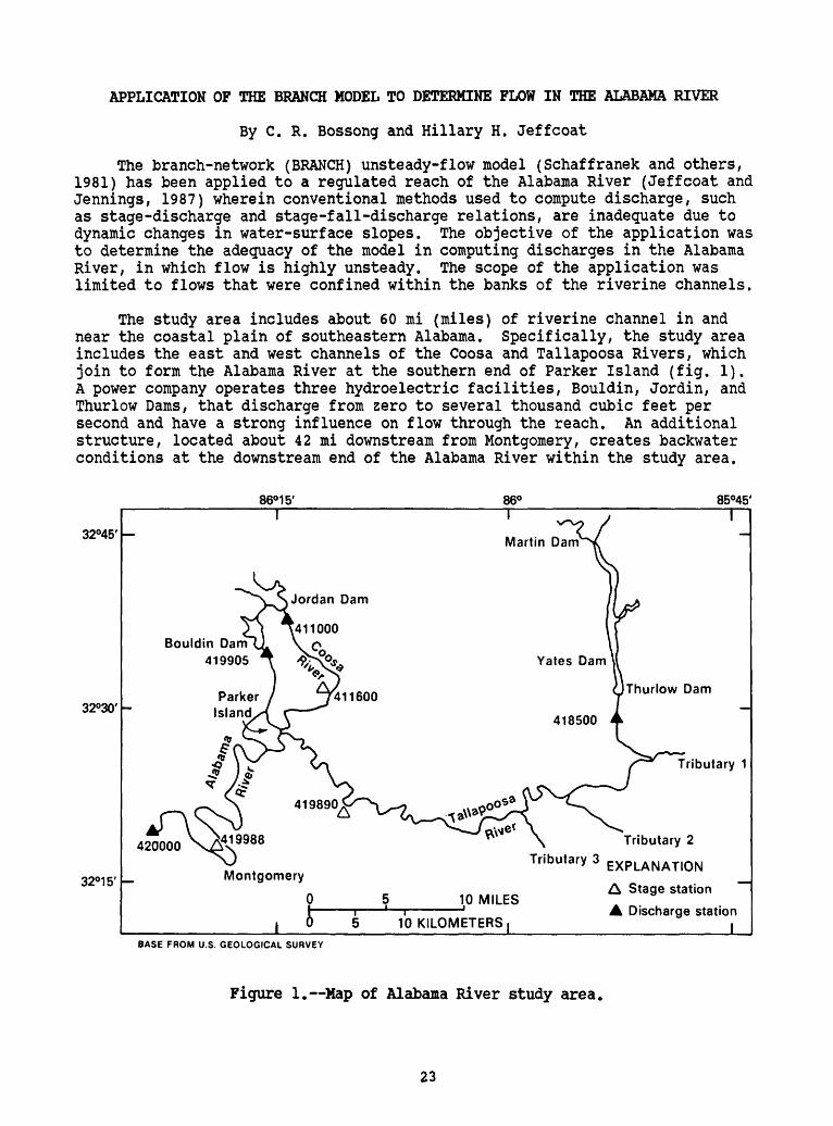
The branch-network (BRANCH) unsteady-flow model (Schaffranek and others, 1981) has been applied to a regulated reach of the Alabama River (Jeffcoat and Jennings, 1987) wherein conventional methods used to compute discharge, such as stage-discharge and stage-fall-discharge relations, are inadequate due to dynamic changes in water-surface slopes. The objective of the application was to determine the adequacy of the model in computing discharges in the Alabama River, in which flow is highly unsteady. The scope of the application was limited to flows that were confined within the banks of the riverine channels.

The study area includes about 60 mi (miles) of riverine channel in and near the coastal plain of southeastern Alabama. Specifically, the study area includes the east and west channels of the Coosa and Tallapoosa Rivers, which join to form the Alabama River at the southern end of Parker Island (fig. 1). A power company operates three hydroelectric facilities, Bouldin, Jordin, and Thurlow Dams, that discharge from zero to several thousand cubic feet per second and have a strong influence on flow through the reach. An additional structure, located about 42 mi downstream from Montgomery, creates backwater conditions at the downstream end of the Alabama River within the study area.

86°15' 86° 85°45'

32°45'

32°30'

32°15'

Bouldin Dam 419905

420000

I

Thurlow Dam

419988

0Montgomery

I

10 MILES

10 KILOMETERS

Tributary 1

Tributary 2 Tributary 3 EXPLANATION

A Stage station

A Discharge station

BASE FROM U.S. GEOLOGICAL SURVEY

Figure 1. Map of Alabama River study area.

23

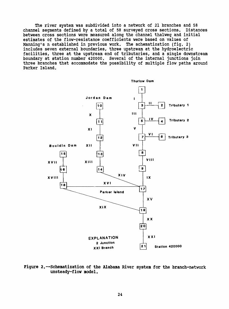
The river system was subdivided into a network of 21 branches and 58 channel segments defined by a total of 58 surveyed cross sections. Distances between cross sections were measured along the channel thalweg and initial estimates of the flow-resistance coefficients were based on values of Manning's n established in previous work. The schematization (fig. 2) includes seven external boundaries, three upstream at the hydroelectric facilities, three at the upstream end of tributaries, and a single downstream boundary at station number 420000. Several of the internal junctions join three branches that accommodate the possibility of multiple flow paths around Parker Island.

Thurlow Dam

Jordan Dam

Tributary 1

Tributary 2

Tributary 3

Bouldln Dam

XVII

XVIII

EXPLANATION2 Junction

XXI Branch

XXI

Station 420000

Figure 2.--Schematization of the Alabama River system for the branch-network unsteady-flow model.

24

Data such as stages, velocities, and discharges at the downstream boundary, stages at various points within the reach, and tributary inflows were available from U.S. Geological Survey records. Much of the additional data required to apply the BRANCH model was obtained from either the U.S. Army Corps of Engineers or the power company. Channel geometry data were supplied by the Corps of Engineers. Top widths of the channels are generally less than 1,000 feet and cross sections vary from relatively shallow profiles with shoals and islands at the head of the reach to deeper and more regular pro files at the end of the reach. The upstream boundary conditions consisted of discharges from the hydroelectric facilities provided by the power company. Boundary conditions for the tributary channels were specified by unit dis charge hydrographs based on runoff correlations. The downstream boundary con dition consisted of stages recorded at 60-minute intervals at station 420000.

The BRANCH model was used to compute flow for a 72-hour period beginning March 7, 1979, by employing a 5-minute time step, a finite-difference weight ing factor of 1.0, and flow-resistance coefficients that varied from 0.035 to 0.050 throughout the branches of the network. Flow-resistance coefficients were determined in calibration efforts in which values were adjusted at individual cross sections to obtain agreement between computed and observed stages and discharges. A limited sensitivity analysis was performed that indicated that the model was sensitive to variations in time step and insen sitive to different values for the finite-difference weighting factor. Sensitivity of the model to changes in segment lengths was not evaluated. Accuracy of the model was evaluated by comparing computed stages and dis charges with observed values at stations 419988 and 420000, respectively. The model was successful in computing hydrographs of similar shape and phase with respect to the observed hydrographs (figs. 3 and 4). Computed discharges are about 10 percent lower than observed values at the highest rates that occurred during the simulation and are slightly out of phase with observed values.

45.000

§ 40.000 oUJ 35,000 V)

LU 30,000 0.

"~ 25.000

O 20,000CDO 15,000zu. 10,000 o< 5.000

ot/2 oQ

-5.000

i i i i i i

EXPLANATION

Observed

Computed

0 5 10 15 20 25 30 35 40 45 50 55 60 65 70 75TIME. IN HOURS

Figure 3. Comparison of observed and computed discharges at station 420000.

25

131

130

129

sCO< 127

jjjt 126

LU(D< 125

124

123

EXPLANATION

Observed

Computed

0 5 10 15 20 25 30 35 40 45 50 55 60 65 70 75 TIME, IN HOURS

Figure 4. Comparison of observed and computed stages at station 419988.

References

Jeffcoat, H.H., and Jennings, M.E., 1987, Computation of unsteady flows in the Alabama River: Water Resources Bulletin of the American Water Resources Association, v. 23, no. 2, p. 313-315.


26

APPLICATION OF THE BRANCH AND LTM MODELS TO THE COOSA RIVER, ALABAMA

By C. R. Bossong

The branch-network (BRANCH) unsteady-flow (Schaffranek and others, 1981) and Lagrangian transport (LTM) (Schoellhamer, and Jobson, 1986a,b) models were applied to a reach of the Coosa River in Alabama. Flow in the reach is regulated and can vary from as little as about 600 to much greater than 30,000 fts/s (cubic feet per second). The Alabama Department of Environmental Management has issued flow-dependent discharge permits for industrial facilities in the reach and, consequently, there is a need for accurate discharge information. Conventional methods used to compute discharges, such as stage-discharge and stage-fall-discharge relationships, have been indequate, especially during periods of low flow, and the BRANCH model has been applied to assess its adequacy. There is also need to increase the understanding of constituent transport properties of the reach so that regulatory decisions may be based on the best possible information. The LTM model has been applied in the reach to assess its adequacy with respect to investigating constituent transport conditions.

The study area consists of a 22-mi (miles) reach of the Coosa River in the Valley and Ridge physiographic province of Alabama, about 35 mi southeast of Birmingham. The main channel is well defined throughout the reach and there is only moderate inflow from relatively small tributaries. A hydroelectric facility which operates at Logan Martin Dam at the head of the reach, discharges from 0 to about 20-30,000 fts/s on a daily basis. A similar facility operates about 25 mi downstream from the end of the reach, which creates backwater conditions in the lower part of the reach.

The reach was schematized into a system of five branches that includes 10 segments defined by a total of 11 cross sections. Distances between cross sections were measured along the channel thalweg and initial estimates of flow-resistance coefficients were based on values of Manning's n established in previous work. The schematization includes an external boundary at the upstream and downstream end of the reach and three internal junctions. Two of the internal junctions are at U.S. Geological Survey gage sites the base gage (02407000) for a slope station located approximately 11.5 mi from the head of the reach and the auxiliary gage (02407040) located about 3.2 mi down river.

Most of the data required to apply the BRANCH and LTM models was collected by the Geological Survey. Data such as stages, velocities, and discharges at the base gage, stages at the auxiliary gage, and tributary inflows were available from Geological Survey records. An additional and temporary, stage gage, established at the downstream end of the reach, was used to define the downstream boundary condition. A power company provided a time series of discharges from Logan Martin Dam which was used to define the upstream boundary condition. Cross-sectional surveys of the channel geometry were conducted using a boat-mounted fathometer. (Channel geometry varies from relatively shallow cross sections with shoals and islands at the head of the reach to somewhat deeper and smoother cross sections downstream. Top widths of the channel cross sections vary from about 500 to 900 ft.) Approximately 2,300 water samples were collected for fluorometric analysis and used to trace the transport of rhodamine-WT dye through the reach.

27

A time step of 15 minutes, finite-difference weighting factor of 1.0, discharge and stage convergence criteria of 100 ft3/s and 0.03 ft, and uniform flow-resistance coefficients of 0.026 were used in the BRANCH model to simulate a 7-day period of flow beginning on October 27, 1984. Calibration of the model was conducted by comparing computed stages, velocities, and discharges with observed values and measured data. Calibration efforts were limited to adjusting the flow-resistance coefficients which were determined to be 0.026 for all channel segments. A limited sensitivity analysis indicated that the model was sensitive to changes in time step but insensitive to different values for the finite-difference weighting factor. The model was not evaluated for sensitivity to changes in channel segment lengths. Although peak discharges computed by the model were lower than those computed with existing ratings, the model was successful in computing hydrographs that closely matched observed values with respect to magnitude, shape, and phase (fig. 1). Measured discharge at 4:00 p.m. on October 30, 1984, falls between the model-computed value and the value determined from the existing rating as shown in figure 1.

30.000

25,000

20.000

15.000

10.000

5,000

-5,000

EXPLANATIONINSTANTANEOUS DISCHARGE MEASUREMENT

NolS «>/* »*» to/so 10/31 IV 1 IV 2

Figure 1. Computed and observed discharges for Coosa river at Childersburg, 02407000.

The LTM was applied to the same channel schematization as the BRANCH model to simulate the transport of rhodamine dye through the reach. The dye injection was treated as a constant-rate injection in the simulation. The model was set up to use a time step of 2 hours, a dispersion coefficient of 0.2, and computed flows from the BRANCH model. A time step of 2 hours was

28

necessary due to constraints of the computer code of LTM and the long period of very low discharges at the beginning of the simulation. The accuracy of the LTM was evaluated by comparing the computed dye concentrations with observed concentrations at the base gage. The simulation period was shorter than for the BRANCH model because, at the time of this application (1984), the LTM could not accommodate negative flows. The LTM was reasonably successful in simulating the magnitude and timing of dye transport to and through the cross section at the base gage (fig. 2).

M

SO

30

20

10

EXPLANATION

OtSEftVED DYE AT HEAD W REACH OISERVED DYE AT 02407000 SIMULATED DYE AT 02407000

2 3DAYS BEGINNING OCTOBER 27,1984, AT 0800 HOURS

Figure 2. Observed and simulated dye concentrations,

References


Schoellhamer, D.H., and Jobson, H.E., 1986a, Programmers manual for aone-dimensional Lagrangian transport model: U.S. Geological Survey Water-Resources Investigations Report 86-4144, 101 p.

1986b, Users manual for a one-dimensional Lagrangian transport model: U.S. Geological Survey Water-Resources Investigations Report 86-4145, 95 p.

29

FLOW DETERMINATION OF THE ARKANSAS RIVER AT LITTLE ROCK, ARKANSAS, USING THE BRANCH MODEL

By Braxtel L. Neely, Jr.

Flow discharges of the Arkansas River are routinely being computed through 15 gates at Murray Dam near Little Rock. These computations are conducted by indirect methods using the geometry of the gates and the upstream and downstream water levels. This approach is reasonably accurate. However, the field equipment presently requires a considerable amount of maintenance and will soon need to be replaced both expensive propositions. The branch- network (BRANCH) unsteady-flow model (Schaffranek and others, 1981) is therefore being evaluated as an alternative streamflow computation method.

The Arkansas River, which traverses the state in west to east direction, is wide with some isolated sandbars throughout the 5-mi (miles) reach being modeled between Murray Dam and the Broadway Bridge in Little Rock. There is very little tributary and(or) lateral inflow within the reach, the southern bank is fairly steep, and a levee exists along the northern bank that is overtopped at high stages. Two branches, defining seven channel segments, are used in the BRANCH model implementation. Eight cross sections, furnished by the U.S. Army Corps of Engineers, define the channel geometry. These cross sections are considered to properly represent the channel properties. Boundary-value data for the model are recorded at the ends of the 5-mi reach. At the upstream end of the reach a float-type gage is located at the down stream side of the locks at Murray Dam. Water stages are digitally recorded every 2 hours from which hourly values are interpolated for use in the model. A manometer-type gage that records digital, hourly, values is situated at the Broadway Bridge. About 5 mi downstream from this gage is another lock and dam system that acts as a control.

Computed discharges from BRANCH seem to be accurate above about 30,000 ft3/s (cubic feet per second), with diminished accuracy below 30,000 ft3/s. (The flow discharge of the Arkansas River is below 30,000 ft3/s about 60 percent of the time.) The free-surface fall between the boundary-condition gages is about 0.08 ft (feet) at a discharge of 30,000 ft3/s. At extremely low discharges, fall between the gages is nearly zero. A typical low-flow period, October 1-6, 1984, shows very erratic stages resulting in negative fall values. Stages are frequently recorded during periods of heavy boat traffic, high winds, or other noisy conditions that adversely affect the instantaneous readings.

The next attempt to evaluate alternative streamflow computation methods for the Arkansas River at Little Rock is to improve the accuracy of the recorded stage data. If this can be accomplished, then further calibration of the BRANCH model will be attempted. Hopefully, these efforts will yield a method for computing discharges within an acceptable level of accuracy.

Reference


3.0

ONE-DIMENSIONAL FLOW MODELING OF THE ST. JOHNS RIVER AT JACKSONVILLE, FLORIDA

By Paul S. Hampson

The St. Johns River originates in a series of marshes almost 300 mi (miles) from its mouth in St. Lucie County, Florida, and traverses north- northwest to Jacksonville, Florida, through a series of lakes roughly parallel to the Atlantic coast. At Jacksonville, the river turns east to the Atlantic Ocean. The length of the river proper is 283 mi with a total drainage area about 8,800 square miles, all of which is contained within the State of Florida. The average gradient of the river is only about 0.1 feet per mile which results in a measurable tidal response as far upstream as Lake George, 106 mi from the mouth. Combinations of north and northeast winds with high tides have occasionally produced flow reversals as far upstream as Lake Monroe, 161 mi from the mouth (Anderson and others, 1973).

Mean tidal range at the mouth of St. Johns River is about 4.9 ft (feet). The range in tide decreases to 1.2 ft at the Main Street bridge, 23 mi from the mouth, and to 0.7 ft at the Jacksonville Naval Air Station, 35 mi from the mouth. Tidal range increases to 1.2 ft from there to Palatka, 78 mi from the mouth, and subsequently decreases to near zero at Lake Monroe (Pyatt, 1964).

Discharge determination in the lower reaches of the St. Johns has always centered around the narrow constriction in the river at downtown Jacksonville (fig. 1). Gaging station 02246500, at the Main Street bridge, was first established in 1954. This is the narrowest and deepest cross section in the lower part of the river, being only 1,320 ft in width with a maximum channel depth of 78 ft. Until 1970, total volumes of flow during ebb and flood tidal periods were computed using the Lobe-area method (Anderson and others, 1973) which utilized two auxiliary gages, one at the Jacksonville Naval Air Station, 8.2 mi upstream from the bridge, and one at the U.S. Army Corps of Engineers dredge depot, 5.0 mi downstream. This method had disadvantages of not providing flow information for specific times, as well as being cumbersome and relatively inaccurate.

In 1970, a mechanical-vane velocity meter was installed 0.3 mi upstream from the Main Street bridge on the Seaboard Coast Line Railroad bridge adjacent to the Acosta bridge (fig. 1). The meter was installed roughly in the center of the span about 250 ft south of the main channel span. A rating of vane response to mean cross-sectional velocity at the Main Street bridge was developed and used to compute discharges until 1974 when it became apparent that the computed discharges were too low. The mean discharge computed for the period January through April, 1974, was -2,000 ft3/s (cubic feet per second). For the same period, the mean discharge for the closest upstream station, 78 mi upstream at Palatka, was 8,000 ft3/s a discharge that was above normal.

In 1978, an electromagnetic velocity probe was installed at the same site as the mechanical-vane meter and a rating was established. The same problem of flow underestimation became evident with the velocity probe.

31

81° 3O° 24-'

81° 35'

^C

JACKSONVILLE

3O° 18'

Cross SectionStation 02246530 St. Johns River at COE Dredge Depot

Cross Section -^,

I Cross Section 3Station 02246500 St. Johns River at Main Street

Arlington Bridge

Fuller Warren Bridge

Cross Section 2

SeaboardCoastlineRailroadBridge

2 MILES i

2 KILOMETERS

Figure l.~Map of St. Johns River study area.

32

In 1985, the decision was made to attempt to compute discharges for the St. Johns River at Jacksonville using the branch-network (BRANCH) unsteady- flow model (Schaffranek and others, 1981). The reach selected for modeling was a 5.0 mi section between the Main Street bridge (station 00246500) and the U.S. Army Corps of Engineers dredge depot (station 02246530). Stage recorders were installed in early 1986 to provide boundary-value data for the model. Because the initial objective of the effort was principally to compute discharges at the Main Street bridge, the first model discretization, as described herein, was kept as simple as practicable with only one branch and three segments bounded by four cross sections. Cross-sectional data were provided by the U.S. Army Corps of Engineers. Future modeling plans are to include the Arlington River (fig. 1) as a side branch with an internal junction at its confluence with the St. Johns River.

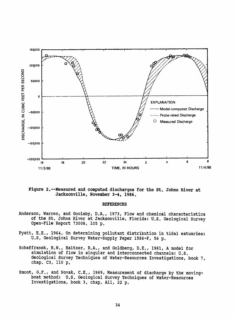
On November 3 and 4, 1986, the first discharge measurements to provide data for calibration of the model were conducted. Measurements were made using the moving-boat method (Smoot and Novak, 1969) along a cross section about 100 ft downstream of the Main Street bridge. Vertical-velocity coefficients were calculated from velocity profile data taken with a Neil-Brown directional acoustic meter at the mid-channel section of the Main Street bridge. Winds during this measurement series were negligible and were not included in the calibration effort. Northerly and northeasterly winds, however, are known to exert significant effects on flow in this portion of the river and will have to be accounted for in future simulation efforts.

The results of the November discharge measurements are shown in figure 2 along with discharges computed by the BRANCH model and those determined from the electromagnetic velocity probe. The BRANCH model results were obtained using a constant frictional-resistance coefficient of 0.0287, a constant momentum coefficient of 1.12, and theta and chi weighting coefficient values of 0.75. The model was found to be significantly sensitive only to changes in the frictional-resistance coefficient.

The preliminary results in figure 2 show that discharges computed from the electromagnetic velocity probe incorporate a phase shift relative to the results obtained from the BRANCH model and do not agree with the measured discharges as well as the model results. Comparison of the shaded areas depicting the difference between model-computed and meter-rated discharges reveals that the electromagnetic-velocity-probe approach underestimates ebb flow volume and overestimates flood flow volume relative to the BRANCH model. The net result is a somewhat consistent underestimation of total flow probably due to placement of the electromagnetic velocity probe 250 ft from the main channel span and in a major bend of the river. Although this source of error is apparent from plots of discharge data as shown in figure 2, it was not readily evident in past velocity-rating attempts.

O O ui

CC LU 0.

fcLU U-

oCO

150,000

100,000

50,000

<-> -50,000

Ul O CC < -100000IO

-150000

-200.00016

11/3/86

,' EXPLANATION

Model-computed Discharge

----Probe-rated Discharge

O Measured Discharge

20 22 24 2

TIME, IN HOURS

6 8

11/4/86

Figure 2. Measured and computed discharges for the St. Johns River at Jacksonville, November 3-4, 1986.

REFERENCES

Anderson, Warren, and Goolsby, D.A., 1973, Flow and chemical characteristics of the St. Johns River at Jacksonville, Florida: U.S. Geological Survey Open-File Report 73008, 105 p.

Pyatt, E.E., 1964, On determining pollutant distribution in tidal estuaries: U.S. Geological Survey Water-supply Paper 1586-F, 56 p.


Smoot, G.F., and Novak, C.E., 1969, Measurement of discharge by the moving- boat method: U.S. Geological Survey Techniques of Water-Resources Investigations, book 3, chap. All, 22 p.

3.4

FLOW MODEL OF SAGINAW RIVER NEAR SAGINAW, MICHIGAN

By David J. Holtschlag

A branch-network (BRANCH) unsteady-flow model (Schaffranek and others, 1981) of the Saginaw River has been developed (Holtschlag, 1981) to provide streamflow data to support solute-transport studies. Original model development was funded through a cooperative agreement between the East Central Michigan Planning and Development Region and the U.S. Geological Survey. The U.S. Environmental Protection Agency subsequently funded flow-model simulations for the 1983, 1984, and 1985 water years.

Saginaw River, which is formed by the confluence of the Tittabawassee and Shiawassee Rivers, traverses through Bay and Saginaw counties in the eastern portion of Michigan's lower peninsula (fig. 1). The river extends northward, and at Essexville, Michigan, connects with Saginaw Bay, an arm of western Lake Huron. The drainage area of Saginaw River is 6,240 mi2 (square miles).

83'45'

Downstreoin model boundary

Weather station A Gaging station .recording

A Gaging station.nonr.cording

US. Geological Survey gaging Site station number

0415705004157046041570370415703204157010041570000415699704156000041515000414900004145000

Base from US. Geological Survey1 : 250,000 maps, 1954 Revised 1971.

Figure 1. Map of Saginaw River and tributaries near Saginaw, Michigan,

35

Saginaw River geometry is regular and has a gradually expanding cross-sectional area in the downstream direction. Width increases from 400 to 800 ft (feet) along the 20-mi (miles) reach that was modeled. The maximum depths at cross sections vary from 10 to 32 ft. Regular channel dredging is employed to maintain a navigational channel downstream from the Geological Survey gaging station at Saginaw (station number 04157000 identified as Site 6 in fig. 1), which is located 3 mi downstream from the confluence of the Shiawassee and Tittabawassee Rivers. The channel bank is protected by riprap throughout much of the modeled reach; small trees and shrubs offer additional bank stability and roughness. Little aquatic growth forms in the river because of its heavy sediment concentration (average of 500 milligrams per liter total solids) and relatively deep channel. Channel bottom material is clay. Partial ice cover is common in the winter.

Stage data have been collected on the Saginaw River at Saginaw (station 04157000) since 1904. Auxiliary water-stage records are collected near Alpin Beach, 19.9 mi downstream (station number 04157050 [new station number is 04157070] identified as Site 1 in fig. 1). A slope rating has been developed for computing discharges greater than 10,000 fts/s (cubic feet per second). (About 10 to 20 percent of daily streamflows can be computed using the slope rating and are reported annually). Lower flows cannot be reliably computed using the slope rating because of unsteady conditions arising from the seiching of Lake Huron. Lake seiching is related primarily to wind conditions on the lake and tidal fluctuations. The variability of the lake levels is high, whereas the wave amplitude is generally low. Typically, hourly stage values near the mouth range less than ± 0.5 ft in a 24-hour period. The range in stage is typically 2.5 ft over a period of 1 month.

For modeling purposes, a schematization depicts Saginaw River as a series of 11 channel reaches or branches. Three additional branches represent the tributaries of Crow Island West Reservoir, Cheboyganing Creek, and Dutch Creek. Branches are further subdivided into segments to better estimate local hydraulic properties. Fifteen junctions delimit or connect the 11 branches. Five external junctions delimit the upstream and downstream boundaries of Saginaw River and the upstream boundaries of the three tributaries. (Either stage or discharge data are specified at the external junctions to simulate flow.) Ten internal junctions connect two or more branches; these permit input of local inflow. An internal junction is also defined on Saginaw River at the outlet of Crow Island East.

The three tributaries that join Saginaw River within the modeled reach have relatively small drainage areas. Cheboyganing Creek has a drainage area of 106 mi2 , Dutch Creek drains 38.3 mi2 , and the Crow Island West Reservoir drains 26.4 mi2 . Although the drainage areas of these tributaries are relatively small, the storage capacities of their lower reaches are important. Therefore, the effects of inflows and outflows within the lower reaches of the tributaries were considered in the flow simulations.

Two small boats were used to collect channel-geometry data for modeling purposes. The first boat was used to set buoys near each shoreline to establish the location of the cross section. This boat crew also measured the

36

channel geometry shoreward of the buoys and the overbank geometry with standard surveying equipment. A reference mark was set on both banks and its elevation relative to the local water level was recorded. The second boat carried a recording fathometer (a sonic depth-measuring unit) that was used to determine the channel geometry between buoys. After the bo^t work was completed, level lines were determined between benchmarks referenced to the International Great Lakes Datum of 1955 and the bank cross-sectional reference marks in order to tie the cross-sectional data to a common reference datum. Fathometer strip charts obtained from the boat were subsequently digitized and composite cross sections were then developed. The near shore and overbank parts of the cross section were combined with the channel segment to complete the cross-sectional profile.

Stage and discharge data at five external boundaries and wind data constituted boundary conditions for the flow simulations. Two of the external boundary-condition requirements were fulfilled by stage data and three by discharge data. Stage data, at 15-minute intervals, were input at the furthest downstream and upstream cross sections of Saginaw River. Average monthly discharges were specified at the upstream end of the modeled portion of each of the three tributaries. Wind speed and direction were measured at two sites one near the mouth and a second upstream, in the City of Saginaw.

The model was calibrated in a two-step process. First, mean monthly flows in the Saginaw River from the model were compared with adjusted mean monthly flows from the gaging stations on the Flint, Cass, Shiawassee, and Tittabawassee Rivers. Initial channel roughness (Manning's n) values were estimated. Minor adjustments in Manning's n values and gage-datum references were applied to produce a match of mean monthly flows over both high- and low-flow conditions. Manning's n values of 0.0235 and 0.0225 were determined for the undredged and dredged channels, respectively, in the calibration effort. Model results were also compared with mean discharges determined from discrete velocity measurements conducted from stationary boats and bridges for periods generally extending from 2 to 4 hours. Comparison of model results and measured values (fig. 2) indicates that the model can accurately simulate unsteady flow in the Saginaw river over the range of discharges analyzed. In the second step, the water-surface drag coefficient of the wind-stress term was varied to minimize differences between measured and simulated instantaneous streamflow values. The relation among the magnitude of the wind-stress term and the accuracy of the flow simulations, as well as the effects of wind conditions on discharges in the Saginaw River, are demonstrated in various plots by Holtschlag (1981). In these calibration efforts, a value of 0.0026 for the water-surface-drag coefficient produced the most accurate model results.

The Saginaw River flow model provides accurate flow computations for open-water conditions throughout the range of discharges normally encountered in Saginaw River. At discharges greater than 10,000 fts/s/ the slope-rating and model results are similar. Additional information and capabilities are needed, however, to compute accurate flows in the winter months when the river is fully or partly ice covered.

37

12,000

10,000

O 8,000UJ CO

uj 6,000

a03D O

UJO cc < I O COQ

Q UJ DCD CO

4,000

2,000

-2,000

-4,000

-6,000

-8,000

-10,000

I I I I

line of agreementx *

Endeco meter measurement

O Price meter measurement

-10,000 -8,000 -6,000 -4,000 -2,000 0 2,000 4,000 6,000 8,000 10,000 12,000

SIMULATED DISCHARGE, IN CUBIC FEET PER SECOND

Figure 2. Relation of simulated to measured discharges of Saginaw River.

References

Holtschlag, D.J., 1981, Flow model of Saginaw River near Saginaw, Michigan: U.S.. Geological Survey Open-File Report 81-1051, 20 p.


38

COMPUTATION OF FLOW AND DETECTION OF THE SALT-FRONT LOCATION FOR THE ATLANTIC INTRACOASTAL WATERWAY (AIW) IN THE VICINITY OF MYRTLE BEACH, SOUTH CAROLINA

By Curtis L. Sanders

The city of Myrtle Beach, South Carolina, plans to augment its water supply by pumping fresh water from the Atlantic Intracoastal Waterway (AIW) in the vicinity of the Myrtlewood golf course (fig. 1). The purpose of this ongoing cooperative project with the city of Myrtle Beach is to determine how much fresh water is available for pumping and to provide a means to alert the pumping station, when it becomes operational, if the salt front gets critically close to the pump intakes.

79°20' 78°40'

34°00' -

33°15'

SPfQFIC CONDUXMIGi AMD

Figure 1. Map of Atlantic Intracoastal Waterway study area in the vicinity of Myrtle Beach, South Carolina.

39

The AIW is open to the ocean approximately 30 mi (miles) south of Myrtle Beach at Winyah Bay and at the South Carolina/North Carolina State line, about 20 mi north of Myrtle Beach (fig. 1). The AIW was modeled from S.C. Highway 544 to S.C. Highway 9, a distance of about 24 mi. South of the study reach, the AIW joins the Waccamaw River, which empties into the Atlantic Ocean at Winyah Bay. The AIW is primarily a manmade channel, about 200 to 260 ft (feet) wide and 15 to 17 ft deep, from the Waccamaw River to the South Carolina/North Carolina State line. For a 4-year period, the maximum, mean, and minimum daily discharges for the study reach were determined to be 7210, 1100, and -216 fts/s (cubic feet per second), respectively.

The Pee Dee River is connected to the Waccamaw River by Bull Creek. The combined drainage area of these two rivers is about 15,000 mi2 (square miles). About 10 to 20 percent of the fresh water from these two rivers flows north to the study reach.

Digital recorders at S.C. Highway 544, Myrtlewood golf course, and S.C. Highway 9 provide stage data for use as boundary values in the model (fig. 1). Nine cross sections were obtained for model implementation by use of a boat-mounted fathometer. Datum of the gages and cross sections were referenced to sea level by standard survey methods.

Specific conductance (sc) is monitored at four sites, temperature at two sites, and dissolved oxygen (DO) and pH at one site (fig. 1). SC gages will be used to alert the city of Myrtle Beach pumping station by telemetry to cease pumping when the salt front is at a predetermined location. Without pumping, the salt front ranges from 7 to 11 mi north of the Myrtlewood golf course (Johnson, 1977).

Flow in the AIW is being determined at the Myrtlewood golf course, in the vicinity of the Myrtle Beach pumping station, by use of the U.S. Geological Survey branch-network (BRANCH) unsteady-flow model (Schaffranek and others, 1981). Three distinct model implementations were developed (S.C. Highway 544 to S.C. Highway 9, S.C. Highway 544 to Myrtlewood golf course, and Myrtlewood golf course to S.C. Highway 9) so that discharges can be computed as long as two of the three stage gages are operational. A 15-minute time step is being used for computations because of the extreme variation of stages in the AIW.

Five sets of current-meter discharge measurements were available for model calibration. Models were calibrated by comparing computed and measured discharges and flow volumes. Statistical programs were developed to compute bias, percent bias, and other statistical indices for computed and measured discharges and volumes. The average percents of bias of the various calibration tests for discharges less than -2000 fts/s and greater than +2000 fts/s ranged from -11.0 to +8.0. The average percents of bias for volumes ranged from -8.6 to +10.5. Each model was calibrated using as many data sets as practicable to validate the results over a wider range of flow conditions, rather than fitting the models precisely for any single set of data.

Statistical programs were developed to produce double-mass curves of flows of the Pee Dee, Little Pee Dee, Lynches, and Waccamaw Rivers compared to flows of the AIW. Double-mass curves were used to detect gross errors in datum or model implementation.

40

Statistical programs also were developed to investigate the relationship between frictional resistance and discharge, however, in the final model calibration, frictional resistance was treated as constant with discharge. Varied frictional-resistance values were used for the open-channel reaches. A frictional-resistance value of about 0.022 was used for the northern reach of the AIW, whereas a value of 0.015 was used for the southern reach. The seemingly low frictional-resistance value in the southern reach could be due to cross-sectional geometry problems steming from imprecisely collected and(or) documented stage and cross-sectional data. This possibility is currently under investigation.

The BRANCH model seems to yield fair results for discharges less than -2000 fts/s and greater than +2000 fts/s. However, flow computations between these two values are poor. Factors contributing to this are low falls between the gages, potential vertical stratification at the northern end of the reach, and difficulties associated with measuring low velocities for calibration use.

The AIW study reach is hydraulically complex because of the combined effects of tides entering at Winyah Bay and at the South Carolina/North Carolina State line and seasonally high freshwater inflows from the Pee Dee and Waccamaw Rivers. Recorded water-surface elevations show that tides propagating from the two open-ocean ends actually pass through each other within the study reach. Because of the rather straight course of the AIW and its predominant northeast alignment, the reach is also highly susceptible to wind effects. Model performance using wind data may therefore need to be evaluated.

References

Johnson, F.A., 1977, A reconnaissance of the hydrology of the intracoastal waterway from Bucksport to Little River Inlet, South Carolina: South Carolina Water Resources Commission, Report No. 7, 33 p.


41

FLOW AND TRANSPORT MODEL OF THE ATLANTIC INTRACOASTAL WATERWAY IN THE GRAND STRAND AREA, SOUTH CAROLINA

By Robert E. Schuck-Kolben

The South Carolina district of the U.S. Geological Survey, Water Resources Division, is currently modeling flow and monitoring water quality in the Atlantic Intracoastal Waterway (AIW). The rapidly growing resort area along South Carolina's Grand Strand, centered around the city of Myrtle Beach, faces severe constraints on local water supply and waste water disposal.

The Black Creek aquifer in the Critaceous Black Creek formation, which has been the primary source of drinking water for the Myrtle Beach area, has a high surface fall rate of approximately 10 feet per year. The city of Myrtle Beach is, therefore, preparing to augment its water supply from a 50-mi (mile) reach of the adjacent AIW that contains fresh water discharged primarily by the Waccamaw and Pee Dee Rivers. The AIW is open to the Atlantic Ocean approximately 30 mi south of Myrtle Beach at Winyah Bay and at the South Carolina/North Carolina State line via Little River, about 20 mi to the north. The Myrtle Beach area also relies on the AIW for disposal of treated waste water and faces problems associated with its limited assimilative capacity as well as the potential for saltwater intrusion if too much fresh water is withdrawn, especially at the wrong locations.

Several years ago, the South Carolina district began implementing the branch-network (BRANCH) unsteady-flow model (Schaffranek and others, 1981) to the northern part of the AIW in an effort to compute mean daily discharges. The present emphasis is to apply BRANCH and the new Branched Lagrangian Transport Model (BLTM) for simulating transport in a network of channels with unsteady bidirectional flow (Jobson and Schoellhamer, 1987)--coupled together to compute flow and transport in the entire reach of the AIW from Little River, South Carolina, to Winyah Bay. The purpose of the modeling effort is to describe the waterway system as accurately as possible with respect to flow and assimilative capacities for optimization of intake and outfall locations. Primary investigations include analysis of low-flow conditions and saltwater intrusion in the entire system as well as determination of mean daily discharges for the northern extremity. Model output will be used to determine optimum instantaneous pumpages and effluent durations.

The Pee Dee River, which is the major tributary to the waterway, is formed in the Appalachian Plateau physiographic province in North Carolina where it is known as the Yadkin River. Within the confines of the study area it is a sinuous, low slope, low-country type of river, and its banks are often flooded especially in late winter and spring. The channel width ranges from 200 to 700 ft (feet) and the average depth is approximately 15 ft within the study area. Upstream of the study area the river is regulated through several small reservoirs, however, flow into the study area can be essentially completely "shut off". The Pee Dee River drains an area of approximately 14,000 square miles and has an average channel slope of 0.79 feet per mile in the reach upstream of the limit of the model. Average discharge of the Pee Dee River for 47 years of record is approximately 9,800 ft3/s (cubic feet per second), making it the major source of freshwater inflow to the system.

42

Other tributaries to the system include the Waccamaw and and Black Rivers which are similar in channel characteristics to the Pee Dee, but drain smaller overall areas. Mean discharges of the Waccamaw and Black Rivers are approximately 1,200 ft3/s and 900 ft3/s, respectively.

Within the confines of the study area to be modeled, the main river channels are relatively straight and range in width from 200 ft in the northern "manmade" reach to as much as 1,500 ft near Winyah Bay at the southern extremity. Branching from these main riverine channels, however, are numerous tidal creeks in a marsh and cypress swamp environment. The potential for overflow into the floodplain almost always exists, but the cross-sectional geometry of the channels is fairly easily defined as a result of their firm and regular sandy bottom configurations. Numerous, treated, waste-effluent outfalls exist throughout the system of channels.

Cross-sectional geometry data have been (and will continue to be) collected using a recording fathometer on a small boat at relatively high slack water. Datum is established for each cross section using a combination of recorded stage data and established tape-down points whereby the mean water level is read and recorded at the site being measured for subsequent reference to NGVD of 1929. Reach lengths are defined for the abundance of tributaries comprising the system. Cross-sectional data will be prepared for model input through use of the Channel Geometry Analysis Program (CGAP) (Regan and Schaffranek, 1985).

Stage boundary-value data are being collected at 20 stilling-well-type gaging stations (including upland gages) equipped with automatic digital recorders actuated by electronic timers.

Ten, four-parameter, water-quality minimonitor stations are strategically located throughout the system for monitoring temperature, specific conductance, dissolved oxygen, and pH. Movement of the saltwater/freshwater interface is identified through use of minimonitor equipment measuring specific conductance and temperature at two depths and two longitudinal positions. Also, longitudinal profiles have been collected on a biweekly basis and during periods of low flow.

Numerous discharge measurements have been made, both by conventional boat measurement techniques as well as by moving boat methods (Smoot and others, 1969). Complex ratings have been established for upstream (inflow) boundaries of the model for verification purposes. These ratings are derived from graphical relations based upon discharges computed from mean velocities determined from index-velocity measurements and cross-sectional areas defined as functions of stage. These discharges are then regressed against upland discharges to determine lag-coefficients and other basin characteristics.

The entire riverine system is affected by a semi-diurnal M2 luni-solar tide of meso-tidal range (-6.5 ft). Reverse highly nonuniform flows exist throughout the system especially during low inflow conditions. The system is well mixed within the model boundaries, but a well-defined salt wedge can develop at the ocean entrances under high inflow conditions. Wind has been shown to have a significant effect upon flows in the currently modeled northern extremity of the system.

43

Prestudy information consisted of topographic maps supplemented by navigation charts with bathymetric data for Winyah Bay. Cross-sectional data were available from the U.S. Army Corps of Engineers for the northern "manmade" reach of the AIW. Extensive reconnaissance of the Winyah Bay estuarine zone and of the hydrology of the northern part of the waterway was done in 1970 and 1977, respectively. Collected data were quite informative in terms of a general overview of the system's characteristics and behavior.

At least 40 years of historical records for the major tributaries are available from upstream gages. Some stochastic modeling was done in 1983-1984 with respect to evaluating the amount of fresh water available for the northern part of the system as a function of combined freshwater inflows. These results were later verified through the relatively successful application of the BRANCH model.

The BRANCH and BLTM models will be used to simulate flow and transport, respectively. The channel schematization will consist of 23 branches, 56 cross sections, and 12 internal junctions. Cross-section locations were selected based upon channel variability and number of junctions as well as with respect to model implementation criteria. The principal output required from the BRANCH model will be low-flow duration and magnitude. BRANCH model results will subsequently be formatted for BLTM input.

Study difficulties encountered have included the setup of leveling equipment in the low swamp conditions of the study area, limited accuracy of discharge measurements during periods of low velocities, extensive overbank conditions that are difficult to quantify, and most of all, at the present time, lack of funding which has been temporarily curtailed.

References


Regan, R.S., and Schaffranek, R.W., 1985, A computer program for analyzingchannel geometry: U.S. Geological Survey Water-Resources Investigations Report 85-4335, 49 p.


Smoot, G.F., and Novak, C.E., 1969, Measurement of discharge bythe moving-boat method: U.S. Geological Survey Techniques of Water- Resources Investigations, book 3, chap. All, 22 p.

44

TIDE-INDUCED CIRCULATION AND FLUSHING USING TIDE GATES IN RESIDENTIAL CANALSOF CAPE CORAL, FLORIDA

By David H. Schoellhamer and Carl R. Goodwin

Cape Coral is a residential development on the western side of the Florida peninsula that contains several tidally affected, autonomous manmade canal systems that have outlets to the Caloosahatchee River near the river's entrance to San Carlos Bay in the Charlotte Harbor estuarine system (fig. 1). Two of these canal systems, referred to as Bluejay and San Carlos, are shown in their entirety in figure 2. The canals range from 100 to 200 ft (feet) in width and from 1 ft or so in depth at many of the dead ends to 30 ft at some locations near the river. The Bluejay canal system also includes several large lakes. Tidal-cycle fluctuations of approximately 1.8 ft at the outlet of the Bluejay system and 1.2 ft at the outlet of the San Carlos system are the primary flow forcing functions. Limited amounts of fresh water enter the San Carlos system at two weir structures (fig. 2) and very little flushing occurs, which can lead to severe water-quality problems, especially in the lakes (D. Morrison, City of Cape Coral, written commun., 1987).

82°10' 82° 81°50'

26°40'

26°30'

5 MILES

5 KILOMETERS

Base from National Oceanic and Atmospheric Administration, Navigation Chart 11427

Figure 1. Location of tidally-affected saltwater canals of Cape Coral, Florida.

45

EXPLANATION

A TIDAL-STAGE SITE LOCATION Z1 AND NUMBER (MODEL BOUNDARY)

A TIDAL-STAGE SITE 22 LOCATION AND NUMBER

Q1

//

/'FW

//

FW

TIDAL-DISCHARGE SITE LOCATION AND NUMBER

FRESHWATER INFLOW SITE

LOCK LOCK SITE

£ BRIDGE

CANAL-SYSTEM BOUNDARY

Figure 2. Schematic of Blue jay and San Carlos canal systems showing stage and discharge measurement sites.

46

Tides in the San Carlos canal system lag tides in the Bluejay system by approximately 2 hours, which results in stage differences between the two systems of half a foot or more for much of the tidal cycle. It is anticipated that this tide difference can be used to improve water circulation and flushing in the canals by the construction of tide gates to permit one-way flow from one system to the other. Tide gates are conceived as being mounted on a horizontal pivot across the width of a channel and are permitted to rotate and allow flow in one direction only. A direct connection between the two systems would generate less tidally-averaged flow (circulation) than a tide gate because the water would oscillate back and forth freely, whereas a tide gate would effectively create a riverine flow through the system during part of the tidal cycle similar to the effect of valves in a human heart. The purposes of this study are to use computer models to estimate the improvement in circulation and flushing that would be created by the use of the tide gates and to determine the optimum tide gate locations.

The procedure used in the study involved calibration and verification of the branch-network (BRANCH) unsteady-flow model (Schaffranek and others, 1981) for existing conditions in the canal system and subsequent numerical evaluation of the effect of proposed tide gates at several potential sites (Schoellhamer, 1988; C.R. Goodwin, U.S. Geological Survey, written commun., 1988). The data-collection effort required the establishment of seven recording stage gages that were operated for several months and the collection of frequent discharge data at five locations (fig. 2) during a 24-hour period in June 1986. The schematic of the canal systems used in the model was simplified from that shown in figure 2 by lumping together several dead-end canals, where feasible. The effect of combining several such canals was tested and found to be negligible. Individual quadrants of the two large lakes in the Bluejay system were treated as channels represented by a wide cross section at the center of each quadrant and two narrower cross sections at the ends. The schematic of the canal system is comprised of 79 branches and 72 junctions. Boundary conditions were tidal stages measured near the two principal outlets of each system. Calibration of the model showed little sensitivity to the frictional-resistance coefficient in the range of 0.023 to 0.029. A single value of 0.026 was chosen for use throughout the network of canals. The model also exhibited stability and little sensitivity to two user-defined weighting coefficients (see Schaffranek and others, 1981) in the range of 0.6 to 1.0. Both coefficients were set to 0.7. Flow simulations were conducted using a time step of 5 minutes.

Model calibration and verification were accomplished by using tidal stage and discharge data. Stage data for June 19-20 were used to calibrate the model. Stage data for June 16-18 and discharge data for June 19-20 were used for model verification (see fig. 2 for site locations). Figure 3 shows the comparison between measured and computed stages in the Bluejay and San Carlos canal systems for June 16-20. The average standard error for the calibration period is 0.026 ft and for the verification period is 0.030 ft. Figure 4 shows the comparison between measured and computed discharges in each system. The standard error ranges from 19 to 59 ft3/s (cubic feet per second), or about 4 percent of the range in discharge at each site. The BRANCH model accurately simulated flow in the existing canal systems; therefore, it was assumed that the model could be used to analyze the effects of hypothetical changes to the systems with reasonable confidence.

47

ttJ

oo

UJ

2.4

2.2

2.0

1.8

1.6

1.4

1.2

1.0

0.8

0.6

0.4

0.2 0

BLU

EJA

Y

SIT

E

Z3

CA

LIB

RA

TIO

N

. .

. I

. .

JUN

E

16

JUN

E

17

JUN

E

18

JUN

E

19

JUN

E 2

0

JUNE 16

JUNE 17

JUNE 18

JUNE 19 JUNE 20

UJ £

2.0

1.6

1.4

0.8

0.6

0'4

u

I

SA

N C

AR

LO

S

SIT

E

Z6

2.0

i/3

1.6

CO

1.2

SJ a

0.8

X z

° 6

a

°-4

^

0.2

'^

0

JUN

E

16

JUN

E

17

JUN

E

18

JUN

E

19

JUN

E 2

0

S/W

CX

lflLO

S

SIT

E

Z5

VE

RIF

ICA

TIO

N

...

I ...

I .

I

CA

LIB

RA

TIO

N

. .

I .

.

JUNE 16

JUNE 17 JUNE 18

JUNE 19

JUNE 20

EX

PL

AN

AT

ION

-----

ME

AS

UR

ED

CO

MP

UT

ED

Figu

re 3.

Sta

ge c

alibration and

ver

ific

atio

n comparisons.

EXPLANATION

COMPUTED MEASURED

1,500JUNE 19 JUNE 20

Figure 4. Discharge verification comparisons.

In order to conduct numerical experiments on the effect of tide gates on water circulation in the canals, a tide-gate algorithm was added to the model. Normal boundary conditions at internal junctions are (1) that the sum of the flow into and out of each junction equals zero and (2) that the associated water stages are equal. Identical conditions were assumed to exist at an internal junction under an open tide-gate condition. For a closed tide gate, the applied boundary conditions are zero discharge through the junction with no constraint on stage. An algorithm to functionally open and close gates was also added to the model. A gate is opened when the stage on the upstream side of the gate is greater than the stage on the downstream side. A parabolic extrapolation algorithm was incorporated in the model to predict impending changes in gate positions.

49

The objective function for optimizing tide-gate locations was to maximize the sum of volume-weighted circulation (tidally averaged discharge) for all reaches in the canal systems. Volume was used to weight the circulation in order to emphasize the need for increased circulation in the large lakes. Eleven possible locations for tide gates that have a width of 10 ft and average water depth of 5 ft were identified and evaluated, and the optimum location for a single such tide gate was found (fig. 5). (Note that a primary flow path through the two systems is established by the tide gate.) The optimum location of a second tide gate was determined by testing 26 possible tide-gate pairs. The optimum pair included the optimum location previously established for a single gate. The optimum locations of up to four tide gates were similarly determined.

The simulated addition of tide gates showed significantly enhanced circulation of water in the canal systems, but the degree of enhancement diminished with addition of each succeeding gate. One tide gate induced a circulation of 168 fts/s. Four tide gates induced a circulation of 279 fts/s, which, over a period of 9 days, yields a volume of water equal to the average volume of water in the two canal systems.

Simulation of constituent transport in the existing canal system is also needed to evaluate flushing. To determine canal dispersion characteristics, a dye-injection experiment was attempted in the Bluejay canal system in June 1986. Unfortunately, a severe thunderstorm occurred shortly after the dye injection, which caused stratified conditions in the canals that invalidated one-dimensional assumptions. Sampling equipment was adversely affected and turbid runoff interfered with fluorometer operation. Nevertheless, a Branched Lagrangian Transport Model (Jobson and Schoellhamer, 1987) was applied that used dispersion characteristics reported in similar canals, but full calibration was not achieved due to the effects of the storm runoff.

A series of numerical experiments were run that used the transport model to determine the relative flushing effects due to tide gates in comparison with the existing no-gate condition. In each experiment, a uniform conservative constituent distribution throughout the modeled region was assumed as an initial condition with no constituent assumed in water at the model boundaries. Results showed that, after 50 days of operation, the computed loss of constituent mass due to flushing was 27, 53, and 79 percent, respectively, for the conditions of no tide gates, one tide gate, and four tide gates. In addition, induced flushing was found to be characterized by a high-rate period for 6 to 10 days following initiation of tide-gate operation, associated with advection in the primary flow paths (see fig. 5), followed by a lower rate associated with dispersive processes in canals adjoining the primary flow paths.

50

EXPLANATION

(§) LOCATION OF FIRST TIDE GATE

TIDE-INDUCED CIRCULATION, -168 IN CUBIC FEET PER SECOND

AND PRIMARY FLOW PATH

/

/

/

/ SAN CARLOS

BRIDGE

CANAL-SYSTEM BOUNDARY

///

/

Figure 5. Flow path and tide-induced circulation for optimum single tide gate

51

References

Jobson, H.E., and Schoellhamer, D.H., 1987, Users manual for a branched Lagrangian transport model: U.S. Geological Survey Water-Resources Investigations Report 87-4163, 73 p.

Schaffranek, R.W., Baltzer, R.A., and Goldberg, D.E., 1981, A model for simulation of flow in singular and interconnected channels: U.S. Geological Survey Techniques for Water-Resources Investigations, book 7 chap. C3, 110 p.

Schoellhamer, D.H., 1988, Simulation and video animation of canal flushing created by a tide gate: American Society of Civil Engineers National Conference on Hydraulic Engineering, Colorado Springs, Colorado, August 8-12, 1988, Proceedings, p. 788-793.

52

EVALUATION OF STREAMFLOW-GAGIHG METHODS FOR APPLICATION TO A RIVER WITH FLAT SLOPE JAMES RIVER, NORTH DAKOTA/SOUTH DAKOTA

By Rick D. Benson and Gregg J. Wiche

The U.S. Bureau of Reclamation is constructing the Garrison Diversion Unit (GDU) which will result in irrigation development of 130,940 acres in North Dakota, 61,145 acres of which will be located within the James River drainage basin. Operation of the GDU has potential to cause substantial changes to the flow regime of the James River at the North Dakota/South Dakota State line. Accurate streamflow computations are required at the State line so that the GDU can be operated to satisfy downstream interests.

An acoustic velocity meter has been installed and the one-dimensional branch-network (BRANCH) unsteady-flow model (Schaffranek and others, 1981) implemented to evaluate streamflow determination techniques on the James River, specifically in a reach of low velocities due to flat-slope variable backwater effects.

The James River extends for 747 mi (miles) from its headwaters in east-central North Dakota to its confluence with the Missouri River near Yankton, South Dakota. It has one of the flattest slopes of any river of similar length in North America the average slope is about 0.6 foot per mile, but is less than 0.1 foot per mile, at certain locations. The James River is characterized by high flows from snowmelt during the spring and from thunderstorms during early summer and by long periods of low flow, or even zero flow, extending from late summer to spring. Major flooding occurs on the James River an average of about once in 10 years, although limited channel capacity at certain locations results in more frequent flooding. During low-flow periods, the velocity is very low as little as 0.1 ft/s (feet per second) at a discharge of 100 fts/s (cubic feet per second).

The study area is located at the upstream end of a former glacial lake bed called the Lake Dakota Plain. The specific reach of study, shown in figure 1, is a 5.3-mi reach of the river extending from the North Dakota/South Dakota State line (station 06470878) to near Hecla, South Dakota (station 06470980). No streams enter the James River within the study reach. The channel width ranges from about 500 ft (feet) at the upstream end of the study reach to about 100 ft at the downstream end. At bank-full capacity, the channel is about 6 to 10 ft deep. The channel-thalweg slope differs between various cross sections, but is about 2 ft throughout the entire 27,920-ft-long reach. Channel bottom material is mostly sandy to clayey lake sediments.

The entire study reach is subject to backwater conditions created by Houghton Dam, a low-head dam located about 10 mi downstream within the Sand Lake National Wildlife Refuge. Since the stage gage was established on the James River at Dakota Lake Dam near Ludden (station 06470875 located about 0.75 mi upstream from the State line) in 1981, the largest recorded discharge has been 2,060 fts/s. However, discharges exceeding 5,000 fts/s have been recorded both upstream and downstream of the study reach prior to installation of the Ludden gage. Average daily wind speeds as much as 12 mi/h (miles per hour) have been recorded at the Ludden gaging station.

53

98 12' R. 60 W. 10' 98 08' R. 59 W.

NORTH DAKOTA

T.129 N.

T.128 N.

Base from U.S. Geological Survey R 61 WGuelph, 1955; Hecla, 1956;Oakes SE, 1955 Q ,/ 1 2 MILES

2 KILOMETERS

LOCATION MAP

EXPLANATION

A°6470875 GAGING STATION-Number is station identification

Figure 1. Location of James River study reach.

54

Discharges at the Hecla gaging-station location have been computed using an acoustic velocity meter (AVM) system with four transducers in a cross-path configuration. The AVM has performed satisfactorily for discharges between about 40 fts/s and bankfull capacity. Accuracy of discharges less than 40 fts/s cannot be determined with any degree of certainty because discrete velocities are less than 0.1 ft/s a rate below the minimum threshold sensing capability of conventional velocity meters.

Discharges at the North Dakota/South Dakota State line have been determined using the BRANCH model. Channel-geometry data required by the model were collected by the U.S. Bureau of Reclamation during the 1985 field season. Stage gages, which consist of float-operated digital recorders actuated at 15-minute intervals at the State line and Hecla locations, provide boundary conditions for the model. A manometer installation at Ludden has been used to define discharges entering the study reach. Wind data (speed and direction) are collected at the Ludden location with a Campbell data logger; instantaneous readings are averaged at 4-hour intervals prior to model input.

For multiple-day simulation periods, special attention was given to the mass-balance aspect of the flow computations, that is, the volume of flow computed by the model was compared to the volume of flow observed during the same period. Model calibration revealed that a flow-resistance coefficient of 0.0268 and a water-surface-drag coefficient of 0.0022 produced the best comparisons.

Figure 2 and table 1 contain comparisons of simulated daily mean discharges at the North Dakota/South Dakota State line to observed discharges at Ludden during July 17 to August 26, 1984, when discharges ranged from 6.4 to 207 fts/s and average daily wind speeds ranged from 1.2 to 12.0 mi/h. For the 41-day simulation period, observed and simulated discharges both averaged 133 fts/s. Observed and simulated daily mean discharges also exhibit close agreement for most of the simulation period. The largest differences between observed and simulated discharges occur during periods of strong, southerly winds. For instance, on July 30 when the average daily wind speed was 11.7 mi/h from almost due south, the observed discharge was 87 fts/s, whereas the simulated discharge was -16 fts/s.

Sensitivity analyses of boundary conditions, model schematization (that is, cross-section locations and channel segment lengths), and simulation time increment were conducted. Stage data at one boundary-condition location were varied in order to evaluate the effects caused by errors in measurement of stages or the effect on flow caused by wind. Analyses revealed that the model is quite sensitive to very slight changes in stage (± 0.02 ft) because of the relatively flat slope of the channel. Analyses of alternate cross sections indicate that the model is also quite sensitive to the channel schematization, especially during periods of strong winds. Sensitivity analyses of the simu lation time increment indicated that a 15-minute interval, which corresponds to the time increment of the boundary-value stage data, produced the best results. Larger time increments were found to yield less-accurate results, probably because of the effects of wind in conjunction with the extremely flat slope of the river.

55

Table 1. Comparison of observed and simulated daily mean discharges for the James River at the North Dakota/South Dakota State line.

Date

July 17, 1984July 18July 19July 20July 21July 22July 23July 24July 25July 26July 27July 28July 29July 30July 31Aug. 1Aug. 2Aug. 3Aug. 4Aug. 5Aug. 6Aug. 7Aug. 8Aug. 9Aug. 10Aug. 11Aug. 12Aug. 13Aug. 14Aug. 15Aug. 16Aug. 17Aug. 18Aug. 19Aug. 20Aug. 21Aug. 22Aug. 23Aug. 24Aug. 25Aug. 26

Ave.

Daily

Observed1

1861271741351211861791671681691701517787

20719917515116817315417516517014798807399

1861561641508044

120100306.4

3056

133

mean discharge(ftVs)

Simulated

20313317413912419117315516215715214625

-1620119916915316115615818217118614876804592

1921481721589665

14212279226892

133

Windspeed(mi/h)

6.43.84.44.66.37.64.12.12.02.01.44.1

12.011.75.86.84.93.32.31.22.26.88.37.52.29.79.4

10.17.44.72.94.63.76.48.86.45.26.1

11.55.75.9

~~

Winddirection

(deg)

32818457

10815126235433817

3361461421601703142070997250

16625128630845

127168175182

0986110

20519527914

163164169183

*At station 06470875, James River at Dakota Lake Dam near Ludden, N. Dak.

56

r

Q 2 O O Ld

Ld Q_h- LJ Ld Lu

300

O CD

O 2

LU O

X O

200

S£ 100 -

-10017

JULY 1984

24 31 7

AUGUST14 21 28

Figure 2. Observecl and simulated daily mean discharges for the James River at th* Hearth Dakota/South Dakota State line, July 17 to August 26, 1984.

In summary, comparison of observed and simulated discharges indicates that it is possible to successfully model the study reach of the James River for flows confined to the main channel and during periods of low to moderate wind. Throughout flow simulations conducted to date, the largest differences between observed and simulated discharges have occurred during periods of strong, sustained southerly winds and during periods when flows have exceeded the bank-full capacity of the channel.

Reference


57

SIMULATION OF FLOW IN THE LOWER CALCASIEU RIVER NEAR LAKE CHARLES, LOUISIANA

By George J. Arcement, Jr.

There is considerable interest in the hydraulic characteristics of the lower Calcasieu River near Lake Charles, Louisiana, especially by managers and officials who regulate the discharge of effluents. To aid these managers and officials, the branch-network unsteady-flow model (Schaffranek and others, 1981) is being evaluated to provide discharge information for the lower Calcasieu River. Water movement in the lower Calcasieu River is an integral function of the configuration of the channel system, freshwater inflow, tidal action, and wind effects.

The lower Calcasieu River extends from about 10 mi (miles) north of the city of Lake Charles to about 35 mi south where it enters the Gulf of Mexico. The study area extends from the saltwater barrier at Lake Charles to about 15 mi downstream to Burton's Landing (fig. 1). The lower Calcasieu River has a 40-ft (feet) by 400-ft wide ship channel maintained to enable deep-draft ocean vessels to reach Lake Charles. A saltwater barrier, located immediately upstream from Lake Charles, is designed to minimize the movement of seawater into the stream channels north of Lake Charles. Between the city of Lake Charles and Burton's Landing there are several cutoffs and three large lakes (Moss Lake, Prien Lake, and Lake Charles which are 1.0, 1.53, and 1.74 square miles in size, respectively) that represent considerable storage area in the waterbody system (fig. 2). The configuration of the many waterways, particularly the 40-ft deep ship channel, permits water to easily move in or out of the river. Headwater streamflow, which must pass through the saltwater barrier, had a maximum rate at Kinder of 182,000 fts/s (cubic feet per second) on May 19, 1953, but generally averages about 2,500 fts/s. Reduced streamflows occur during the June through November period.

Tidal action is the dominant factor in water movement in the lower Calcasieu River. Three kinds of tide can occur with a diurnal pattern being dominant. The diurnal tide range at the mouth is about 2 ft. Total flow can occur in either direction in the channel and stratified flow can develop under certain conditions with freshwater inflow moving downstream in the top layer and seawater moving upstream in the lower layer. This potential stratified flow condition poses particularly difficult problems in use of the one-dimensional, cross-sectionally averaged, model.

The branch-network unsteady-flow model has been used to simulate continuous discharges at several locations in the study reach. Flow was simulated through the lakes as well as through the ship channel using the model. The study reach shown in figure 2, represented by 29 cross sections, was divided into 13 branches for purposes of model implementation. Four representative cross-sectional profiles are illustrated in figure 2. Cross-sectional depths for model development were obtained using a fathometer. Widths were derived from topographic maps for the lakes and were field measured for the channel cross sections. Boundary conditions for the model consisted of stages collected hourly at the saltwater barrier and at Burton's Landing, with wind data also being collected at Burton's Landing. Both stage gages were referenced to a 1984 adjusted benchmark network.

5.8

STUDY AREA

^r

JEFFERSON DAVIS

SALTWATER, A I Goosport

30°10'

Base from U.8. Geological Survey State base map, 1:500,000 10 MILES

I I I0 5 10 KILOMETERS

Figure 1. Location of lower Calcasieu River study area.

I I I I ICross section 2

Thalweg «l«v. -40.10 ft.

Ill III

0 200 400 600 DISTANCE FROM LEFT BANK. IN FEET

I I I I I I I Cross section I 0

Thalweg (lev. -41.50 ft.

! I I I I I I I I

DISTANCE FROM LEFT BANK. IN FEET

0 200 400 600 800

DISTANCE FROM LEFT BANK. IN FEET

I I I I I ICross section 30 Thalweg (lev.

-38.40 ft.

EXPLANATION200 400 600 600 1.000

DISTANCE FROM LEFT BANK. IN FEETCross section number

A 08017035 Gaging station and USGS downstream order number

Mile 39 River mile above mouth

Figure 2. Location of study reach, gaging stations, and representative cross-sectional geometry.

Eight sets of discharge measurements, ranging from 48,100 to -32,300 fts/s, were used to calibrate and verify the model. Measurements were made at an upstream site on a railroad bridge below the saltwater barrier and also at Burton's Landing (see fig. 2). These discharge measurements were made using a directional velocity meter. The model was calibrated at a 15-minute time step, but daily discharges were computed using a 60-minute time step with little difference being observed in the final results. Calibration runs were made using five sets of discharge measurements. The average error for the calibration runs was 13.9 percent. Three sets of discharge measurements were used for verification with a resultant average error of 29.6 percent. The sizeable error of the verification runs can partly be attributed to the typically lower discharge periods in which flow stratification occurred. A higher flow-resistance coefficient was required to simulate the net discharges during stratified flow conditions. The resultant flow-resistance coefficient, defined as a function of discharge and developed for model purposes, ranged from 0.014 to 0.36.

Although the model error is significant for discharges computed during stratified flow conditions, no other practical method is currently available to compute daily discharges in the study reach. It is fully recognized that the lower Calcasieu River is a very complex flow system and is difficult to represent by a one-dimensional model. Daily flow computations, however, are essential for proper management of the waterbody system. Therefore, use of the one-dimensional branch-network model will continue to be evaluated and, hopefully, improved. An additional problem area encountered in using the model, which will require further analyses, is how to appropriately account for the significant storage capacity of the lakes.

Reference


6JL

BRANCH FLOW MODEL OF THE KNIK AND MATANUSKA RIVERS, ALASKA

By Stephen W. Lipscomb

A study of the combination riverine-estuarine reach of the Knik and Matanuska Rivers has been conducted by the U.S. Geological Survey to provide hydrologic and hydraulic data to the Alaska Department of Transportation and Public Facilities (ADOT&PF) for use in the design of additional bridge crossings of the two rivers.

The Knik and Matanuska Rivers both originate at large glaciers in the Chugach Mountains and empty into Cook Inlet about 40 mi (miles) northeast of Anchorage. Glenn Highway crosses these rivers in their tidally influenced lower reaches. Tides can induce as much as a 10 ft (feet) rise in stage in the lower reaches of the rivers, whereas their upper reaches are not tidally influenced. The Knik River reach is 7.3 mi long and has a fall of about 15 to 20 ft over that distance. The Matanuska River reach is 11 mi long and has a fall of more than 150 ft. Both reaches are characterized by a complex system of interconnected channels that meander across a 2-mi-wide floodplain. Several overflow channels that are dry during low and medium flows become wetted during high flows. Bed material consists of coarse sand and gravel; the channels are subject to some deposition and erosion.

Glacier outburst floods, caused by the natural damming and subsequent release of Lake George behind the Knik Glacier, occurred annually on the Knik River until 1967. These events produced peak discharges an order of magnitude greater than those associated with non-breakout years. The entire floodplain in the vicinity of the study reaches is inundated by glacier-outburst flooding. Recent studies of the Knik Glacier indicate that the potential remains for future glacier advance and reformation of Lake George.

The U.S. Geological Survey branch-network (BRANCH) unsteady-flow model (Schaffranek and others, 1981) has been used to evaluate the hydraulic characteristics of the Knik-Matanuska River system. Implementation of the model required input of cross-sectional geometry data at critical locations throughout the network of channels as well as time series of boundary-value stage and(or) discharge data at the upstream and downstream extremities of the study reaches. These data were collected during the 1984 and 1985 summer field seasons and subsequently reduced to a format compatible with the model's input requirements. Model output is in the form of simulated flow discharges and water stages at the extremities of the reaches as well as at intermediate locations where channel geometry is specified.

Cross-sectional geometry data were obtained using standard field survey techniques on the banks and a recording fathometer for the in-stream portions. Datum was provided throughout the study reach by the ADOT&PF. Cross-sectional geometry data were reduced for input to the model using the Channel Geometry Analysis Program (CGAP) (Regan and Schaffranek, 1985).

Stage data were collected at the six external boundaries of the network using either mercury manometers or pressure tranducers. Stages were recorded at either 30-minute intervals on punched-paper tapes or at 15-minute intervals using electronic dataloggers. Solid-state timers were used for all recorders

and timing was synchronized and checked frequently, especially before and after each set of measured data was collected. Time-dependent boundary-value and calibration data were processed and prepared for input to the model using the Time-Dependent Data System (TDDS) of programs (Schaffranek and Baltzer, 1978; Lai and others, 1978).

Three sets of discharge data were collected for calibration and verification purposes. These data were obtained in the lower tidally influenced reaches. Each set of data included discrete measurements of velocities and depths at several predetermined locations within the cross section throughout an entire tidal cycle. Velocity and depth data were then used to compute instantaneous discharges at 15-minute time intervals.

Intermittent flow in the overflow channels posed a problem in model implementation. This condition was accommodated by altering their configurations to include an artificially deepened thalweg or 'spike 1 . These deepened sections were constructed so as to be of negligible area, thereby maintaining the integrity of the channel conveyance properties while satisfying the model's implementation requirements and assumptions.

At times during flow simulations it was observed that the artificially deepened channels were conveying significant flows and causing some undesir able circulation patterns and fluctuations of stages within the network. This instability was most pronounced at lower flows and made calibration of the model in this range difficult. Because one objective of developing the model was to provide a tool for the analysis of flood flows, it was determined that calibration of the model in the higher ranges of stage was most critical. For this reason, model calibration concentrated on high stages only.

Of the three discharge data sets for calibration only two proved to be useful. The third set was of less utility due to the fact that it was obtained during a period of relatively low flow.

Calibration efforts yielded computed discharges within 10 percent of measured values. Simulations made to verify the model indicate that further calibration could improve the accuracy of simulated results.

Various sensitivity tests were performed to facilitate verification and efficient use of the model. For example, the simulation time step was varied from two to fifteen minutes and simulation results were compared in an effort to minimize model run time. Several simulations were conducted to test the affect of excluding certain branches from the model schematization. Those branches with the potential for going dry during the simulation were deleted from the model as an alternative to adding artificially deepened thalwegs as discussed previously. Incrementally altering various features of the model schmatization and comparing the affects on computed results, provided a useful, verified, tool for conducting flow simulations.

Several simulations were conducted after altering the channel geometry files to synthesize hypothetical redesign conditions at the lower bridge sites. These changes were made to reflect various proposed bridge configurations. Results from simulations were provided to ADOT&PF to aid in optimizing the bridge design.

6.3

References

Lai, Chintu, Schaffranek, R.W., and Baltzer, R.A., 1978, An operational system for implementing simulation models, a case study: American Society of Civil Engineers Specialty Conference on Verification of Mathematical and Physical Models in Hydraulic Engineering/ College Park, Maryland/ August 9-11, 1978, Proceedings, p. 415-454.

Regan, R.S., and Schaffranek, R.W., 1985, A computer program for analyzing channel geometry: U.S. Geological Survey Water-Resources Investigations Report 85-4335, 49 p.

Schaffranek, R.W., and Baltzer, R.A., 1978, Fulfilling model time-dependent data requirements: American Society of Civil Engineers Coastal Zone '78 Symposium on Technical, Environmental, Socioeconomic, and Regulatory Aspects of Coastal Zone Management, San Francisco, California, March 14-16, 1978, Proceedings, p. 2069-2084.


FLOW DETERMINATION FOR OHIO RIVER AT GREENUP DAM AND LOUISVILLE, KENTUCKY

By Kevin J. Ruhl

The branch-network (BRANCH) unsteady-flow model (Schaffranek and others, 1981) is being used by the Kentucky District of the U.S. Geological Survey, Water Resources Division, to compute average daily streamflows at two sites on the Ohio River; one at Greenup Dam and another at Louisville. The Greenup Dam site at river mile 342 was established in 1968. Until 1981 flow was computed using hydraulic formulae for flow through a control structure. The method was converted to a slope-station computation technique in 1981 and an auxiliary gage was established 14 mi (miles) downstream from the dam and base gage. Daily discharges were computed using the slope rating for two years. In 1984, the BRANCH model was implemented on the reach defined for slope-station computation. The Louisville station was established in 1928. From 1970-85 a slope-rating method was used to compute flow with the auxiliary gage being located at Kosmosdale, approximately 20 mi downstream from the dam and base gage. Since 1985 the BRANCH model has been used to compute daily discharges.

The flow of the Ohio River which borders Kentucky is regulated by a series of high-lift dams. The Ohio River between the sites at Greenup Dam and Louisville averages about 0.25 mi wide expands to greater than 0.75 mi in width at certain locations. The bottom material is generally compacted sand and gravel. Stages range from 12 to more than 40 ft (feet) and the fall in the reaches ranges from 0 to 6 ft. Flow extends into adjacent overbank areas only during extreme discharge events. No significant inflow occurs in either of the study reaches. Tygarts Creek and Little Scioto River drain into the Greenup Dam reach, but the drainage areas of these two streams are only 340 and 230 mi2 (square miles), respectively. The drainage area of the Ohio River at Greenup Dam is approximately 62,000 mi2 .

Cross-sectional data for the Greenup Dam reach were obtained from a consultant's report for the U.S. Army Corps of Engineers. Cross-sectional surveys were taken at intervals ranging from 0.5 to 1.5 mi apart and were referenced to NGVD Datum of 1929. Channel-geometry information for the Louisville reach was obtained using cross-sectional data from the Corps of Engineers and from soundings taken across the channel at 0.25-mi intervals. These soundings were supplemented with topographic information to produce cross-sectional geometry data for model input. For input to the model, cross-section locations were selected at approximately 1-mi increments throughout the Greenup Dam reach. Cross sections for the Louisville reach were selected based on the change in bank-full conveyance; the cross sections chosen averaged about one per mile.

The base and auxiliary gages at Greenup Dam are of the stilling-well type. The base gage at Louisville is a stilling-well type and the auxiliary gage is operated using a manometer. Recorders at all four gages are actuated on one-hour cycles and all are equipped with backup systems. Discharge measurements are conducted approximately four times per year at each site.

A value of 1.0 was used for the momentum coefficient and values of 0.7 were used for the finite-difference weighting factors for both model implementations. Optimum flow-resistance coefficient values for each of a number of discharge measurements were determined by trial and error adjustment and comparison of simulated and measured discharge values. Flow-resistance coefficient values were then plotted against measured discharges and average coefficient values were obtained for use in the calibrated models. For the Greenup Dam model, a variable flow-resistance coefficient was defined for flows less than 90,000 ft3/s (cubic feet per second).

Generally, at both sites, discharges computed using the calibrated BRANCH model compare very well with those computed from the slope rating. Average daily discharges computed using the two methods generally agree within 5 percent, except during periods when the flow is less than approximately 50,000 ft3/s. Some discharges computed in this range at the two sites differ by more than 10 percent. A study has been initiated to compare discharges computed using the model at the Louisville site when the number of cross sections in the reach is varied, but results at this time are inconclusive.

Reference


66

FLOW MODEL OF THE HUDSON RIVER FROM ALBANY TO NEW HAMBURG, NEW YORK

By David A. Stedfast

The Hudson River traverses to the south and east from its headwaters in the Adirondack mountains of northern New York to Glens Falls, where it begins its 180-mi (mile) southward course to New York City (fig. 1). The Hudson River estuary, which extends 150 mi from New York City north to Troy (fig. 1), is a major navigation channel and source of water supply for several municipalities and industries.

This entire reach is affected by tides as evidenced by the large variation in stages and discharges over a tidal period at any particular location. The mean tidal amplitude at New York City is 4.5 ft (feet) and upstream at Troy the mean amplitude is 4.7 ft. The direction of flow in the estuary reverses four times daily as far north as Albany, 3 mi south of Troy, except during the high inflows of spring that overshadow the tidal influences. Maximum flood and ebb discharges during a tidal cycle typically range from ±20,000 fts/s (cubic feet per second) at Albany to ±250,000 fts/s at Poughkeepsie.

Tidal influences cause highly erratic flow patterns that cannot be defined by standard gaging methods. Until 1981, data on streamflow in the estuary could only be determined by adding average monthly discharges of the Hudson River at Green Island near Troy (U.S. Geological Survey gage 01358000), which is not tide affected, to calculations of monthly inflows from the downstream subbasins. Increasing demands placed on the Hudson River for water supply and waste disposal, countered by a demand to preserve it for recreation and wildlife use, created a need for detailed knowledge of the magnitude and variability of flow in time and space.

The objective of this investigation, undertaken by the U.S. Geological Survey in cooperation with New York State Department of Environmental Conservation and the New York City Department of Environmental Protection, was to develop, calibrate, and verify a computerized transient-state model that could provide discharge, stage, and direction of flow at any specified time and cross section between Albany and New Hamburg (fig. 1) the approximate northern limit of saltwater conditions. The results of this investigation, which began in late 1977, are discussed in Stedfast (1982).

The 76-mi reach of the Hudson River from Albany to New Hamburg was divided into two subreaches near the midpoint at West Camp (fig. 1) to simplify model calibration. A separate model was developed for each subreach using the general purpose, one-dimensional, finite-difference flow-simulation model developed by Schaffranek, Baltzer, and Goldberg (1981). Sensitivity analyses were conducted for each of these subreach models to ascertain the optimum channel geometry schematizations, simulation time increments, computational iteration controls, and finite-difference weighting factors. Additional sensitivity analyses were also conducted to provide base information for model calibrations.

6.7

30'

74°30' 74° 73°30'

GREEN IS. DAM_4/ri,o>

Glens Falls

RENSSELAER

J

J«CASTLf TON -ON -HUDSON

Poughkeepsie

New York

30'

41°

0 5 10 MILESI H-, 0 5 10 KILOMETERS

ATLANTIC OCEAN

Base from U.S. Army Corps of Engineers, 1962

Figure 1. Location and major geographic features of the Hudson River.

6-8

The northern subreach, the 41-mi stretch from Albany to West Camp (fig. 1), contains several tributary and side-channel storage areas. Channel characteristics of this subreach vary significantly from north to south and only 8 percent of the contributing drainage area is gaged.

Three discharge measurements were available to calibrate and verify the model representing the Albany to West Camp subreach. Observed and simulated discharges for this subreach are shown in figure 2. (Negative discharges represent upstream flow during the flood cycle of the tide.) Simulated maximum flood and ebb discharges for August 21, 1979, at Albany (fig. 2a) were within 5 percent of observed discharges and the simulated net volume of flow over a full tidal cycle was within 25 percent of the volume computed from observed data. Discrete simulated discharges, for this period of low inflow conditions at Green Island (August 21, 1979), differed considerably, however, from observed discharges near flow reversal and resultant hydrographs were 15 minutes out of phase. These differences were attributed to the sensitivity of

25

20

15

10 -

o ao9 Ot-

* -5

-15

-20

-25

« Computed value

o Observed value

K «

I I I10 11 12 13 14 15 16 17 18 19 20

TIME OF DAY. IN HOURS

(a)

Figure 2a. Observed and computed discharges at Colonie St. Bridge, Albany, August 21, 1979.

60

50 -

o 40 -

30 -

20

10

000

« « o ««, o

« o o o o o o««oo oooo __«o ««ooooo

« o

« o

o « o

o « o «

« Computed value

o Observed value

I I I I

10 11 12 13 14 TIME OF DAY, IN HOURS

15 16 17

250

200 -

§150*-

O CO

Oo 50

20-

|-50

-100

-150

« o o «* «

* _ o « o

o o «O « -K

o _ «

o « «o * «

Computed value

Observed value

18 19

I I I .1 I I

10 11 12 13 TIME OF DAY, IN HOURS

14 15 16 17 18 19

(c)

Figure 2b, 2c. Observed and computed discharges: b, at foot of Maiden Lane, Albany, March 26, 1980; c, at a point 2.5 miles south of Rip Van Winkle Bridge, Catskill, April 18, 1980.

70

the model to tributary inflow (only 8 percent of the contributing drainage was gaged), side channel storage, and(or) effects of wind shear. These sensitive model conditions would be especially noticeable during low-flow periods. Simulated discharges of March 26, 1980, (fig. 2b) and April 18, 1980, (fig. 2c) which represented high inflow conditions at Green Island, agreed in phase and did not differ significantly from observed discharges. Simulated discharges of March 26, 1980, at Albany were within 13 percent of observed discharges and the net volume of flow over a tidal cycle was within 2 percent of the volume computed from observed data. Simulated maximum flood and ebb discharges of April 18, 1980, at Catskill, 34 mi south of Albany, were within 3 percent of observed discharges and the simulated net volume of flow over a complete tidal cycle was within 4 percent of the volume computed from observed data.

The southern subreach, the 35-mi stretch from West Camp to New Hamburg (fig. 1), differs significantly from the northern subreach in that the channel characteristics do not vary as substantially and 88 percent of the contributing drainage area is gaged.

Four discharge measurements were available for calibration and verifi cation of the model representing the West Camp to New Hamburg subreach. Observed and simulated discharges for August 21, 1979, are shown in figure 3. During calibration of this model, tributaries and other side-channel storage areas were determined to affect flow to a far lesser extent than in the northern subreach and were, therefore, not represented in the final combined model schematization. Maximum flood and ebb discharges at both Rhinecliff (fig. 3a) and Poughkeepsie (fig. 3b) were within 6 percent of observed discharges and mean simulated flood and ebb discharges were within 9 percent of the mean of observed values. However, the simulated and observed net volumes of flow over a tidal cycle at these sites differed by as much as 100 percent as a result of the small magnitude of net flow in relation to the large cumulative flood and ebb volumes of flow. Nevertheless, the simulated values were within the limits of field-measurement accuracy for observed data.

After the subreach models were calibrated and verified, the channel schematizations for both were combined to form a model of the entire reach from Albany to New Hamburg.

Nine sets of discharge measurements were available to verify the model five at Poughkeepsie, two at Albany, and one each at Red Hook and Rhinecliff (fig. 1). Flow simulations for August 21, 1979, and March 26, 1980, produced maximum flood and ebb discharges at Albany that were within 6 percent of observed discharges and simulated flow volumes over a tidal cycle that were within 2 percent of volumes computed from observed data. Simulated maximum flood and ebb discharges at Red Hook, Rhinecliff, and Poughkeepsie were within 10 percent of the observed discharges for all but the May 24, 1966, measurements.

Flows at Poughkeepsie were also simulated for the entire month of September 1978 to enable comparison between long-term computed outflow and computed freshwater inflow from Green Island and the intervening subbasins. The simulated mean discharge at Poughkeepsie for the month was 7,510 fts/s, which is within 10 percent of the calculated inflow of 6,900 fts/s.

71

10

HJ H-

*9

DIS

CH

ARG

E. I

N T

HO

US

AN

D C

UB

IC F

EET

PER

SEC

ON

D

R

4 L

L *

c»<D

8

88

08

82

VI

------

w e> w

«

1W

W O

"**

1

M*

tf*

PI

W

(D*J

S *^

vj

**<

§

(S1

A*

*d a

o p

* p^

K

rT* 2

J? o

o

s<0

M

O

M

M>

£H

- ft

S

<D 0

(t>

_,

*

*1

Pi

s_

H

- £

if P

I P

i *-

+.

O -

fiO

|^.

j t

-n

K>

<0

M ^ g

"

&

ft >

P

|

Z3

CO iQ

iQ

P

-M

MM

t»-

=VO

N

>>

J M

0

)V

O-

-

enM

M

VO

>J

Ul

*ft

&*

H^

<0

_.W

>*

rt

W &

Ru

ft

*"tf^

i PJ

*

A o

C2

M>

£

M O

1 1

1 1

1*

o *

*0

*

f f

0**

~"

5 1

o *

»

a 0 *

0.

Q.

0

^

0 *

g s

° *

0 *

"~

0

* ~

~0 *

0 *

0 *

-

o *

0

*0 *

0*

o*

-0

*0* 0

~

0

~0

00

-

*o

0

*0 0

-

*o

~*0

*0*0

* o

"~*

0 *0*

o

* o

*

0 * 0

* 0

~~

* 0

~~

*0 *0 *0

"~

«o

~~0

00 *

~~

0

* ~

0

*0

* 0

*

**

1 1

f 1

1

§

DIS

CH

ARG

E. I

N T

HO

USA

ND

CU

BIC

FEE

T PE

R SE

CO

ND

,

00 <0 o

^ _

fn

^~*

oA

l "^

>

> ."*

w

^

_.a

* 0̂1

O)

o _. * 5 *

--

1 1

1 1

1 1

1*

o *

*0

*

If

o-°*

c

o*

*

0*

V

&

&

V

< <

°i i

0S

S o

00*

~

0*

0*

0*

o*

0 *0 *

0~

*

o -

* 0 *

0 0

0

~

0 *

0 0

0

~~0

0Q

*0*

~~0 *

0*

0* 0

* 0 * 0*

_

o* 0 0* 0 *0 *

**

1 1

1 1

1 1

1

Past studies have indicated that strong north and south winds, in particular, have a significant effect on the Hudson River (Busby and Darmer, 1970). Although the Hudson River model was not calibrated to account for this effect due to lack of data, an evaluation of hypothetical wind conditions indicated that a sustained 10 miles per hour north wind during low flow could increase peak southward flow at Albany by as much as 25 percent and decrease the northward flow by a similar quantity. The analyses further indicated that both the tidal phase and amplitude would be substantially affected.

References

Busby, M.W., and Darmer, K.I., 1970, A look at the Hudson River estuary: Water Resources Bulletin, v. 6, no. 5, p. 802-812.


Stedfast, D.A., 1982, Flow model of the Hudson River estuary from Albany to New Hamburg, New York: U.S. Geological Survey Water-Resources Investigations Report 81-55, 69 p.

73

SIMULATION OF DEBRIS FLOWS USING THE HYDRAUX MODEL

By R. Peder Hansen

Because debris flows pose a potential life-threatening hazard and can cause considerable damage, it is important to understand their characteristics and be able to predict their magnitude. Debris flow dynamics can differ significantly from one event to another as well as within a single event. Even though debris flow characteristics can be markedly different from "clear water" flow, much information has been generated by using streamflow models to simulate debris flows. This approach was adopted to simulate lahars (volcanic-originated debris flows) on Mount St. Helens.

Early debris flow modeling efforts by the U.S. Geological Survey in studies on Mount St. Helens used a general purpose dam-break flood simulation model, called DAMBRK, as originally formulated, developed, and documented by Fread (1977) and subsequently modified and documented by Land (1981). Although the DAMBRK model uses conventional techniques for numerical solutions, instabilities developed resulting in model failure whenever flows of very high magnitude, sharply rising peak discharges were routed in steep channels. In the present study, a one-dimensional unsteady flow model, called HYDRAUX, was used (Delong, 1986). Both DAMBRK and HYDRAUX solve the one- dimensional, unsteady flow equations, albeit by different numerical methods.

It is necessary to compare model results with well documented events to evaluate the use of a streamflow model in the simulation of debris flows. On March 19, 1982, a lahar with an initial peak discharge at the crater of about 14,000 ft3/s (cubic feet per second) flowed down the North Toutle River in Washington (fig. 1). This lahar which is used for model demonstration purposes is described in detail by Pierson and Scott (1985), whose report contains much of the velocity and timing information needed to test a

46°22'30" -

________Ib"________________122"________

( c = EXPLANATION s$r (^ & WASHINGTON __^*S \ Al PHI Landslide-

- \ '& '"^ debris avalanc

__^\ /« &%% Landslide- V <? ^' ^ dejjris avalanche

^-B.STUPYAR6A MM Mod "ow

-

0240 KILOMETERS

Figure 1. Map of North Toutle River study area,

74

66

LJJ

LJJ C/)

LJJ

O CD

LL

LJJ O

C/)iccLJJ

64

62

60

58

56

Modeled

Modeled calc n= _ .020 - .037

012345

ELAPSED TIME FROM PEAK AT KID VALLEY, IN HOURS

Figure 2. March 19, 1982, hyperconcentrated flow at Highway 99 Bridge.

75

numerical model of a debris flow. (Two other reasonably well documented lahar events, which occurred following the major eruption of Mount St. Helens on May 18, 1980, also have been simulated and recently documented. Details of this effort are contained in Laenen and Hansen (in press).)

The HYDRAUX model is used without calibration to simulate debris flows employing calculated Manning's "n" values. Manning's "n" values are calculated at cross sections where peak water-surface elevations are known and the mean velocity is determined either from a rating extension (at stream gaging locations) or by superelevation or run-up formulas. A discharge hydrograph is used as an upstream boundary condition. No other boundary conditions are imposed. The upstream discharge-hydrograph shape and volume are estimated from available documented evidence. Cross-sectional geometry data are kept fixed for the duration of the model run and Manning's "n" is considered constant with time and depth at each section. No attempt was made to adjust model input to achieve a better fit to observed data.

Model results were compared with observations from three events. Accuracy was defined by comparing model results to known peak arrival times and elevations. Figure 2 shows the comparison between recorded and modeled results at the Highway 99 Bridge, 22.4 miles downstream from Kid Valley, as well as the input hydrograph for the March 19, 1982, event. The input hydrograph at Kid Valley shows a peak discharge of 960 ft3/s. Two scenarios were simulated; one using calculated "n" values and a second using a typical clear water "n" value for the same reach. A complete summary of the project and model results are presented by Laenen and Hansen (in press).

References

DeLong, L.L., 1986, Extension of the unsteady one-dimensional open-channel flow equations for flow in meandering channels with flood plains, in Subitzky, S., Selected Papers in The Hydrologic Sciences: U.S. Geological Survey Water-supply Paper 2290, p. 101-105.

Fread, D.L., 1977, The development and testing of a dam-break flood forecasting model: Dam-Break Flood Routing Workshop, Hydrology Committee, U.S. Water Resources Council, Bethesda, Maryland, Oct. 18-20, 1977, Proceedings, available from U.S. Department of Commerce, National Technical Information Service, Springfield, Virginia 22151 as report PB-275 437, p. 164-197.

Laenen, A., and Hansen, R.P., in press, Simulation of three lahars in the Mount St. Helens area, Washington, using a one-dimensional, unsteady- state streamflow model: submitted for publication in Water Resources Research.

Land, L.F., 1981, User's guide for a general purpose dam-break flood simulation model (k-634): U.S. Geological Survey Water-Resources Investigations Report 80-116, 101 p.

Pierson, T.C., and Scott, K.M., 1985, Downstream dilution of a lahar:transition from debris flow to hyperconcentrated streamflow: Water Resources Research, v. 12, no. 10, p. 1511-1524.

76

APPENDIX I

Glossary of Technical Terminology

Part of this glossary of technical terminology, common to the field of computational hydraulics, was prepared, initially, for use at the Advanced Seminar on One-Dimensional, Open-Channel Flow and Transport Modeling. Subsequently, additional terms were included as a result of the Seminar discussions and proceedings. It is hoped that the glossary will be helpful in clarifying technical terms commonly used in computational hydraulics in relation to numerical modeling of unsteady open-channel flow. It is also anticipated that consistent and precise usage of generally accepted, or "standard", terminology will foster improved communication among technical personnel of related fields. This collection of technical terms was selected for the above-mentioned purpose; it was not intended to be an exhaustive listing of all terminology in the field of computational hydraulics.

In preparing the glossary, the chapter "Numerical Modeling of Unsteady Open-Channel Flow" (Lai, 1986) in "Advances of Hydroscience" (v. 14) edited by V.T. Chow and B.C. Yen, has been relied upon. In particular, table 1: Unsteady open-channel flow equations; table 2: Explicit finite-difference schemes; and table 3: Implicit finite-difference schemes, contained in this APPENDIX, are transcribed with some minor modifications from Lai (1986).

Other key references, which were consulted and(or) included: Chow, 1959; Cunge and others, 1980; Dronkers, 1964; Henderson, 1966; Mahmood and Yevjevich, 1975; Parker, 1983; and Rantz and others, 1982.

REFERENCES

Chow, V.T., 1959, Open-channel hydraulics: New York, McGraw-Hill, 680 p.

Cunge, J.A., Holly, E.M., Jr., and Verwey, A., 1980, Practical aspects of computational river hydraulics: London, Pitman, 420 p.

Dronkers, J.J., 1964, Tidal computations in rivers and coastal waters: North-Holland Publishing Company, Amsterdam, 518 p.

Henderson, F.M., 1966, Open channel flow: New York, Macmillan, 522 p.

Lai, Chintu, 1986, Numerical modeling of unsteady open-channel flow, in Advances in Hydroscience: Chow, V.T., and Yen, B.C., eds, Academic Press, Orlando, Florida, v. 14, p. 161-333.

Mahmood, K., and Yevjevich, V., eds., 1975, Unsteady flow in open channels: Fort Collins, Colorado, Water Resources Publication, v. 1 and 2, 923 p.

Parker, S.P., ed., 1983, Dictionary of scientific and technical terms (3rd ed.): New York, McGraw-Hill, 2662 p.

Rantz, S.E., and others, 1982, Measurement and computation of streamflow: Volume 1, Measurement of stage and discharge; Volume 2, Computation of discharge: U.S. Geological Survey Water Supply Paper 2175, 631 p.

77

Table 1. Unsteady open-channel flow equations11 [From Lai, 1986, table I]

Conditions (a) Equation of continuity (b) Equation of motion

1. Equation sets using depth h and velocity u as dependent variables

(i) Basic form, general cross section

(ii) Basic form, general cross section

(iii) Prismatic channel

(iv) Nonprismatic channel with lateral inflow

(v) Wide nonprismatic channel with lateral inflow and wind stress

dA d

dt dx

dh vA du

dt dx dx

dh dh du

dt dx dx

dh dh du u dA

dt 'dx dx B dx H

dh dh du dAB + uB + A + u dt dx ox dx

d d dh + . s _s}-Q dt dx ' dx

1 du u du dh _ -t- -t- J0 -r Jf " g dt g dx dx

du du dh

dt dx dx

q du du dh q(u u')

B dt dx dx A

du du dh q(u - u')

k "* " dt r " dx """ * dx a"° T A

-t?f a*0 = 0

2. Equations sets using depth h and discharge Q as dependent variables

(vi) Conservation form

(vii) With lateral inflow

(viii) With lateral inflowand wind stress

~Pl + fix = °

*£ + £-«

dh dQ

dt dx

dQ d ( Q 2 \ d --T + I~ [ft T + 0 M*) + 9A(S, - S.) = 0 dt dx \ A ) dx

dQ Q dQ d fQ\ dh

dQ fQ\ ^Q d (Q\ c^dt \Aj dx dx \A/ dx

- gA(S0 - S,) - qu' - ZBVlcost) = 0

3. Equation sets using stage Z and velocity u as dependent variables

(ix) Prismatic channel

(x) Nonprismatic channel

(xi) Nonprismatic channel with lateral inflow [/»=!]

(xii) Nonprismatic channel with lateral inflow, wind stress, and Coriolis effect [/»=!]

dZ dZ du du du dZ + M + H + uS0 = 0 + u + 0 + gS, = 0 dt dx dx dt dx dx

dZ dZ du d B + uB + A + u- dt dx dx d

dZ dZ du u dA\ + u + // + - dt ex dx B dx \

dZ dZ du u dA

A d d 2 dZ

x ,, dt dx dx f

q du du dZ q

> ° B dt dx dx ' A

du du dZ q + u + g + gSf + -(u - u) ot dx dx A

vi ~ /7" cosdZ Vi

q + 2(o,u ̂ sin 0 = 0 dy h

in the transverse direction

4. Equation sets using stage Z and discharge Q as dependent variables

(xiii) Basic form, general cross section

(xiv) With lateral inflow[/>= U

(xv) With lateral inflow.wind stress, and Coriolis force [ft - U

dZ dQ B + _* = odt dx

dZ dQ

dt dx

dZ dQ

dt d.x

dQ I Q \ dQ d i Q\ dZ + /^[ 1 + fiQ I 1 + qA + f/ASr = 0 ft \AJdx dx\Aj ' dx

3Q Q C Q f iQ\ fZPl + AP\ + dx\A) + g dx +a' ' qU

fQ Q fQ f (Q\ fZdt A ex ?X\A) g dx

+ gAS, - qu' - £BV*cosO = 0dZ Q V 2

q + 2w.- - c---sintf = 0 rv 'A ' h

in the transverse direction

"A few new syntols are defined as follows: k'.wind speed; 0 angle of wind direction with+.x direction; wz vertical component of earth's rotation; h depth from the water surface to the centroid of the cross section.

78

Table 2. Explicit finite-difference schemes [From Lai, 1986, table II],

Computational grid-point structure Unstable Diffusive

L-shaped (upstream) Leap-frog Lax-Wendroff

structure * + i-| 1 U A--H-I <

( ) Unknown t j j | L [k T T I T (o, x) Known | 1 1 1

A/ /-I / /+! /-I ;

I £

i U *+i-

6- * ,

i /+ 1 /-

|

1 jH/

h *+ 'H>- k-4

* ' * 1

/' 1

-1 /

r /-

r * '/-H i

H-i >Hy^rKl

' xi~ xi-\

2 Ax

Discretization expressions

d/ A/

2A~7

A/

or * Wf ~ W?-\

A/

2 A*

2 A/

Depends on PDE s used; commonly includes

2 Ax

(Ax)

. VV:

Wf or f K . \*/ n

Discretization error

Table 3. Implicit finite-difference schemes* [From Lai, 1986, table III],

Computationalgrid-pointstructure Box Rectangle Wide flange Tee

( ) Unknown

(o) Known

-6- *-

AW w**\-w*.^ wf.t-w? wAY'^/V ^ML ~ e ^±j y_ + (,- e)_i±j /_ e j±j /_L + ( ,_ fl) .a* Ax Ax x/ + l~ ;fy-l

The some os rectangle schemes

aw .. ,<i'-<i u , ,.<L < .,.<*' <'. X-V-^-i - » * + (\~\i/i rf> + { \-(b< Discretization expressions dW_ !Vi_JVl (| _ , 'U_

di At A/ ^ A/ " T A/ A/ A/

The same as rectangle schemes

m which 05<e5lO,0<^ <| 0, in which x, -*,.(

0 < x < 1 0

" Discretization error varies with values and combinations of weighting factors. Aside from stability and other numerical and physical considerations, better accuracy is usually obtained by a more symmetrical arrangement.

79

A

Alternating flow. See Unsteady flow, alternating.

Average depth (H). See Hydraulic depth.

B

Backwater curve. a term used primarily to indicate the longitudinal surface profile of the water backed up above a dam, other control, or into a tributary by flood water in the main stream. See also, Flow profile of steady gradually varied flow.

Body-force term. See Unsteady open-channel flow equations, term [9],

Boundary condition. a requirement that the dependent variable of a differential equation must satisfy along a boundary of the solution domain.

Boundary-value data. specified values for a dependent variable at given values of the independent variable(s).

Boundary-value problem. a problem which involves finding the solution of a differential equation or set of differential equations that satisfy certain specified requirements, usually connected with physical conditions, for certain values of the independent variables. [This notion is directly extendable to solution of finite-difference equations in the case of numerical modeling.]

Boussinesq coefficient (B).--See Momentum coefficient.

Box scheme.~a numerical discretization for the implicit finite-difference method (FDM) utilizing four points, two on the current and two on the advanced time lines, spaced one grid cell apart. [See Table III.] Has advantages of simplicity in computational grid-point structure, flexibility of placing variable weights on various grid points, and applicability to unequal distance intervals. Also known as Preissmann or four-point scheme.

C

Celerity. See Wave, celerity.

Characteristic method. See Method of characteristics.

Chezy's C. also, Chezy coefficient. The factor in the Chezy formula that accounts for the flow resistance.

8.0

Chezy formula. also, Chezy equation. An equation f or^ the velocity, f U, of steady, uniform open-channel flow: U = (VK5 in which C is the Chezy coefficient, R is the hydraulic radius, and So is the bed slope.

Continuity equation. an equation obeyed by any conserved, indestructible quantity such as mass or energy (head in hydraulics), which is essentially a statement that the rate of increase of the quantity in any control region equals the net influx of the quantity into the region. Also known as Equation of continuity.

Convergence. See Numerical convergence.

Convective [acceleration] term. See Unsteady open-channel flow equations, term [7].

Conveyance. a measure of the carrying capacity of a channel section expressed as K = Q/V5 wherein Q is the discharge and S is the slope of the energy grade line in steady flow.

Convolution method.~a computational method using a convolution of two functions. If the two functions are f(t) and g(t), then their convolution is denoted by (f*g) = J* f(T)g(t-T)dr.

Coriolis

~ acceleration. an acceleration which, when added to the acceleration of an object relative to a rotating and moving coordinate system and to its centripetal acceleration, gives the acceleration of the object relative to a fixed coordinate system.

~ effect. the effect of the Coriolis force in a rotating system. For the rotating earth, this effect is manifested by the deflection of a moving object or flowing water on the earth's surface. [An object moving hor izontally is deflected to the right in the Northern Hemisphere, to the left in the Southern. This is to say that, for a river in the Northern Hemisphere flowing toward the West, Coriolis force generates super elevation (higher water-surface elevation) on its northern bank.]

~ force. a velocity-dependent pseudoforce in a reference frame which is rotating with respect to an inertial reference frame; is equal and opposite to the product of the mass of the particle on which the force acts and its Coriolis acceleration.

Coriolis coefficient (a). See Energy coefficient.

81

Courant

~ condition. also, Courant-Friedrichs-Lewy (CFL) condition. The usual condition for stability of the explicit formulation of a numerical scheme that requires that the ratio (Cr ) of the propagation speed of a physical disturbance to that of a numerical signal should not exceed unity, that is Cr « 1.

- constraint. the limitation derived from the Courant or CFL condition.

- number (Cr ). the ratio of physical wave celerity T ( = dx/dt = u±c in which ur is the flow velocity in the x direction and c is the wave celerity) to computational celerity r ( = Ax/At in which AX and At represent finite space and time quantities for computations), that is, C = r/r = (u±c)/(Ax/At). [The Courant number for other types of characteristics may be similarly defined or derived. For example, the Courant number for the single characteristic case of transport problems may be expressed as Cr = u/(Ax/At).]

Dam-break flow. unsteady flow resulting from a dam failure. [Although it can range from flow caused by instant and total collapse of a dam to that induced by gradual breaching of a dam, dam-break flow is often classified as rapidly-varying unsteady flow.]

Darcy-Weisbach [resistance] coefficient (f). also Weisbach frictionfactor, Weisbach resistance coefficient. The flow resistance coefficient used in the Darcy-Weisbach formula for pipe flow analysis. [Because of its dimensionless form, use of this coefficient is often extended to open- channel and other types of flow.] It is related to Chezy's C and Manning's n as l/Vf~= C/VBg = (XR^J/^Bg n) in which g is the acceleration of gravity, R is the hydraulic radius, and x = 1 and 1.486 for the international and inch-pound systems of units, respectively.

Datum. any numerical value or geometric quantity (such as a point, line, surface, or horizontal plane) that serves as a base reference for other quantities or values (such as bathymetric soundings, ground elevations, water-surface elevations, etc.).

Debris flow. a flowing mixture of water and sediment that has sufficient yield strength to exhibit plastic flow behavior, such as the forming of flow fronts or lateral levees and suspension of gravel-sized particles, and yet remains or becomes partially liquefied. [In contrast to hyperconcentrated flow, when a debris flow comes to rest, it will consolidate at the rate at which fluid can drain out of the mixture. Fine and coarse particles settle together without interparticle movement.]

Diffusion analogy. also, Diffusion-analogy approximation. See Noninertial approximation.

82

Diffusion [wave] model. also, Diffusion-analogy model. See Noninertial approximation.

Diffusive scheme.~a numerical discretization for the explicit FDM. [See Table II.]

Discharge (Q).--the volume of water that passes through a cross section of channel within a given period of time.

Discretization error (6). For w(x,t) and W(x,t) representing, respectively, theoretical (exact) solutions of the partial differential and difference equations for each fixed point (x,t), then the difference, that is, 6 = W - w, is termed the discretization error. Also referred to as truncation error, discretization error is preferred inasmuch as the word truncation connotes the idea that W can be represented by a power series of, say Ax, which is not always the case. Also easily confused with round-off error.

Domain of dependence. Determination of the values of unsteady flow variables at any point P(x,t) within the region of existence of the solution, depends entirely on conditions within the triangle-like area APB that is, bounded by two intersecting characteristics C+ (SF) and C_ (EP), and the line connecting point A (xx ,t ) and point B (x2 ,t2 ), where A and B are earlier points in time, that is, t1<t, t2<t. This area is called the domain of dependence of P. See also "Range of influence."

Double-sweep method. a numerical computational method frequently used to solve a linear system of equations implicitly. In application to an open-channel reach, the computation procedure sweeps the reach twice: using information given at one boundary-condition location and proceeding to the other boundary, incorporating the imposed boundary condition there, and then completing the solution process in a return sweep.

Dynamic [wave] equation. See Dynamic wave equation(s) 1.

Dynamic wave

~ equation(s).--l. The conventional equation of motion. 2. Thestandard set of unsteady open-channel flow equations including both the equations of continuity and motion. [The term is often used to dis tinguish the equations from simplified equations such as kinematic, noninertial, or steady dynamic equations.] Also, Saint-Venant equations. See Unsteady open-channel flow equations.

~ model. a numerical model based on the dynamic wave equations.

83

Ebb flow. flow in the downstream direction in a tidal river or estuary. Also, ebb current. See also "Flood flow 2."

Energy coefficient. a coefficient quantifying the variance of velocityfrom a uniform distribution across the channel section in application of the conservation of energy principle. [For fairly straight prismatic channels the energy coefficient varies from about 1.03 to 1.36. A value of unity implies that the velocity is strictly uniform across the channel section.]

Energy equation. an equation expressing the conservation of energy in a channel section, in which contributing effects are customarily expressed in units of length called "head."

Equation of continuity. See Continuity equation.

Equation of motion. an equation based on Newton's second law of motion, Fx = max (where F is force in the x direction, m is mass, and a is acceleration in the x direction), namely, stating that the resultant force acting on a body is equated to the time rate of change of momentum in the body.

Estuary. 1. The downstream portion of a riverine channel or system of channels, a naturally occurring waterway, or a semi-confined waterbody leading to or connecting with the open ocean in which measurable physical evidence of the ocean tides cyclic fluctuations in water levels and unsteady flow velocities are discernible. 2. The downstream portion of a riverine channel or system of channels, a naturally occurring waterway, or a semi-confined waterbody leading to or connecting with the open ocean in which a threshold concentration of ocean salt is discernible, or within which seawater is measurably diluted with fresh water.

Eulerian

~ equation. the form of equation of motion based on Eulerian concepts, in which a fixed coordinates system is used and tangential and normal stresses accompanying deformation are ignored.

* approach. an approach premised on Eulerian concepts and a fixed coordinates system.

Explicit finite-difference method. a numerical method for solvingfinite-difference equations explicitly, (usually) on a rectangular grid system. Dependent variables on the advanced time level are determined one point at a time from known values and conditions at grid points on the present time level, or, present and previous time levels. [Several numerical schemes belonging to the explicit FDM are summarized in Table II.]

84

Finite difference

~ approximation. representation of differential forms of equations (continuum) by corresponding finite difference forms (discrete quantities).

~ equations (FDE). equations derived by substituting difference quotients for derivatives in differential equations.

- method (FDM).--an approximation method in which finite difference expressions are substituted for differential equations in order to effect a solution.

Finite element method (FEM). an approximation method for studying continuous physical systems, often used in structural and fluid mechanics, involving tasks of discretizing the system or domain into a number of finite elements interconnected at discrete nodal points, analytically or numerically integrating the product of approximating functions and weighting functions, and numerically integrating (over time) the resultant equations on the computer.

First-order approximation. a numerical result approaching the exact solution to the first degree. Also, linear approximation.

Flood flow. 1. Flow discharge during a flood. 2. Flow in the upstream direction in a tidal river or estuary. Also, flood current. See also "Ebb flow."

Floodplain. the relatively smooth, level, land adjacent to and along an alluvial river channel that is subject to being submerged by overflow from the main channel.

Flood routing. the process of computing the progressive time and shape, that is, hydrograph, of a flood wave at successive points along a river channel. Also, storage routing, stream routing, flow routing, streamflow routing.

Hydraulic . also, hydraulic method of flood routing. This method is based on solution of the basic differential equations for unsteady open-channel flow.

Hydrologic "". also, hydrologic method of flood routing. This method makes no direct use of the basic differential equations for unsteady open-channel flow, but approximates their solution in some sense using hydrologic concepts.

85

Flow profile. also, Longitudinal profile, Water-surface curve.

~ of steady gradually varied flow. a nonuniform longitudinal profilethat forms when a channel configuration or a hydraulic structure affects a uniform flow (steady case) or when there is a transition from one state of uniform flow to another. [Twelve types of such a flow profile or water-surface curve have been identified; these curves are relatively flat and change only gradually (except near critical or other control points). Characteristically, these flows have negligible vertical velocity components. Among hydraulic engineers, they are also called "backwater curves" if the flow depth increases, and "drawdown curves" if it decreases, in the downstream direction. As a group, they are often referred to as "backwater curves".]

~ of steady rapidly varied flow. a highly nonuniform, longitudinal water- surface profile that appears in flows via hydraulic structures, past channel transitions, through hydraulic jumps, and around sharp bends. [Such flows are characterized by a large curvature in profile, sudden changes in flow direction, and/or nonnegligible vertical or lateral components of flow velocity or acceleration.]

~ of unsteady gradually varied flow. a time-dependent, nonuniform,longitudinal flow profile. [As in the steady case, such a surface curve is relatively flat, and changes only gradually, but in both space and time. ]

~ of unsteady rapidly varied flow. a highly variable, spatially and temporally, longitudinal water-surface profile present in unsteady rapidly-varied flow, such as dam-break flow or flow in a steep channel, moving hydraulic jump, surge, bore, etc.

Flow-resistance coefficient. a coefficient quantifying the mean shear stress on flow in open channels. For unsteady flow, the flow resistance coefficient is usually approximated from that used in the steady flow case. The cross-sectionally averaged velocity, U, of an open-channel flow varies with the bed slope, So , the hydraulic radius, R, and the flow resistance coefficient, C. For a turbulent uniform flow, the most practical formula can be expressed in a general form U = C Rm SJJ in which C is represented by C in the Chezy formula and as x/n (where x = 1 and = 1.486 for the international and inch-pound systems of units, respectively) in the Manning formula.

Flow-resistance term. See Unsteady open-channel flow equations, term [10].

Flushing characteristics. a measure of the displacement of water (often laden with dissolved or suspended constituents) from a riverine or estuarine system as governed by the combined action of freshwater inflow and tidal exchange.

Flux. the movement of some quantity, for example, mass or volume of fluid, sediment particles, other dissolved or suspended constituents, flowing or passing through a given area (often a unit area perpendicular to the flow, for example, the channel cross section) per unit time.

86

Four-point [implicit] scheme. 1. A numerical solution scheme belonging to the implicit FDM; variables at the four corners of a rectangular cell are used for finite difference expressions. Also called the Preissmann or box scheme (See Box scheme 1.). See Table III. 2. Any numerical scheme belonging to the implicit FDM which uses four grid points for finite dif ference expression.

Free-surface flow. 1. In hydraulics, the water flow in flumes, open channels, waterways, embayments, seas, etc., for which the water surface is exposed to the atmosphere. 2. In fluid mechanics, the free-surface means a boundary between two homogeneous fluids.

Froude number (F). 1. A dimensionless number used in the study of fluid mechanics, representing the ratio of a unit inertial reaction to a typical unit force due to gravity. 2. In open-channel flow, the Froude number is signified by the ratio of the speed of flow (u) to the speed (celerity) of a very small gravity wave (c); that is, F = u/c = u/VgE in which h is (a characteristic) depth of flow.

Gaussian elimination method. a numerical tool (or a numerical computational method) used to solve a set of simultaneous linear equaitons. By successive combinations of equations, all elements in the coefficient matrix below the diagonal are eliminated to form an upper triangular matrix, after which the unknowns are determined by successive back substitution.

Gradually varied flow. flow in which the depth along the axis of the channel changes gradually.

H

Head of tidewater. the maximum upstream extent of tidal influence with respect to (a) saltwater intrusion; (b) flow reversal; or (c) flow unsteadiness (due to tidal action). [Often, only case (c) is referred to.]

Hydraulic depth (H). also known as "Average depth". The depth obtained by dividing the cross-sectional area of flow normal to the flow direction (A) by the channel top width (B), that is, H = A/B.

Hydraulic radius (R). also termed the "Hydraulic [mean] radius". It is defined as the quotient of the cross-sectional area of flow (A) and its wetted perimeter (P), that is, R = A/P. [In a wide open channel this amounts to about the average depth of flow, and in a circular pipe flowing full, this is equal to one quarter of the pipe diameter.]

Hydrograph. a graphical representation of flow characteristics, that is, stage, discharge, velocity, etc., at a given point as a function of time.

87

Hyperconcentrated streamflow. a flowing mixture of water and sediment that possesses a small but measurable yield strength and still appears to flow like a liquid. [In contrast to a debris flow, when a hyperconcentrated flow comes to rest, particles settle out of suspension and are deposited separately depending on their fall velocities.]

Hysteresis. See Loop rating curve.

Implicit finite-difference method. a numerical method for solving finite difference equations (commonly) on a rectangular grid system. For a basic set of difference equations, a number of unknown variables are placed on a multiple number of grid points at the advanced time level that are related to less-weighted known values of dependent variables at the present time level. The solution proceeds implicitly by simultaneously solving the resultant system of equations. [Several numerical schemes belonging to this method are summarized in Table III.]

Initial condition. a prescription of the state of a dynamical system at some specified time; for all subsequent times the partial differential equations describing the system and boundary conditions determine its state.

Initial-value data. In initial-value problems, if numerical data are given for certain values of the independent variable as the initial conditions, such data are referred to as initial-value data.

Instability. a condition of a control system in which excessive positive feedback causes persistent, unwanted, oscillations in the output of the system.

Hydrodynamic (or hydraulic) ~. 1. Hydrodynamic or hydraulic instability can occur due to natural phenomena (with no relation to the equations derived to describe the flow); for example, roll waves, surges, steep channel flows, transitions between supercritical and subcritical flows, nonhomogenous (or stratified) flows, etc. 2. Hydrodynamic or hydraulic instability can result from the differential equations used to represent the flow conditions (the actual flow might or might not be unstable). The assumptions made for, or the technique used in, deriving the equations can contribute to such instabilities.

Numerical ~. A numerical scheme is considered stable if the total error, E, the difference between the theoretical (exact) solution of the partial differential equation, w, and^the numerical solution of the corresponding partial difference equation, W, will not grow unbounded in successive computations. [This is usually analyzed by testing whether W will be bounded or not, assuming that w is stable (that is, hydrodynamically stable).]

88

Junction. a point of intersection of conduits (open or closed), waterways, or their subdivisions. For convenience and generality, the terminal end of a reach is sometimes also referred to as a junction.

K

Kinematic wave. a wave in which discharge is a function of depth alone. [In open channel flow this implies that the friction slope, S., is equal to the bed slope, S , and that the other slope terms in the equation of motion (cf. unsteady open-channel flow equation II.) are negligible.] The existence, and form, of such a wave can be shown from the equation of continuity, thus bearing its name, "kinematic wave."

Kinematic wave approximation. an approximative method for modeling unsteady open-channel flow using kinematic wave theory; that is, using the equation of continuity only and assuming that discharge is a function of depth alone.

Lagrangian approach. an approach premised on Lagrangian concepts; that is, the concern is focused on what happens to individual fluid particles in the course of time, what paths they describe, what velocities or accelerations they have, and so forth.

Lateral inflow/outflow. 1. The flow, or flow component, in the direction normal to the longitudinal or principal flow direction. 2. The flow entering or leaving the side of a conduit or channel.

Lax scheme. also, Diffusive scheme. A numerical scheme of the explicit FDM, which is based on the following approximation of derivatives:awat At aw- *Eu - w*., ax 2AxIf « = 0, the form reduces to that shown in Table II, and if « = 1, it reduces to the unstable scheme shown in Table II.

Lax's equivalence theorem. the theorem that states, "Given a properly posed linear initial value problem and a finite difference approximation to it that satisfies the consistency condition, stability is the necessary and sufficient condition for convergence."

Lax-Wendroff scheme. a numerical solution scheme belonging to the explicit FDM. Unlike other explicit FDM schemes, the Lax-Wendroff scheme uses nonlinear variation for finite-difference approximations to improve the computational accuracy. See Table II.

89

Leap-frog scheme. a numerical solution scheme belonging to the explicit FDM. This scheme uses three time levels, instead of two as in many other schemes, for temporal finite-difference expression. See Table II.

Local acceleration term. See Unsteady open-channel flow equations, term [6].

Loss coefficient. coefficient accounting for head loss at entrances, exits, junctions, etc. of open channels or conduits.

L-shaped differencing scheme. See "Upstream differencing scheme." See Table II.

Loop rating curve. In unsteady flow, there exists more than one discharge value for a given stage value, the resulting stage-discharge curves (rating curves) thus exhibit loops and kinks, and are often referred to as "loop rating curves". The loop rating curve generated by a typical simple single-peaked flood flow may resemble an air-foil shape.

M

Manning formula. one of the most commonly used steady, uniform-flowequations for open channels; also known as strickler's formula in Europe. For water flowing with velocity U in a channel of bed slope SQ and hydraulic radius R, the formula can be expressed as U = (x/n)R2/3SQ 1/ 2 ; in which n is Manning's roughness coefficient and \ = 1 and 1.486 for the international and inch-pound systems of units, respectively.

Manning's roughness factor (n). also called "Manning's roughnesscoefficient." Coefficient used in the Manning formula characterizing the surface roughness of the channel under steady flow conditions; often referred as Manning's n.

Method of characteristics (MOC). 1. In applied mathematics, the method of characteristics signifies a mathematical approach to solving initial- boundary value problems by first transforming the original partial differ ential equations representing the system into corresponding characteristic equations equations and then delving into a mathematical treatment of the transformed equations. The physical interpretation of this is that instead of analyzing the unsteady flow from the viewpoint of an observer at a fixed location for a given moment, the flow is analyzed from the viewpoint of an observer moving with the wave crest or with the characteristic. 2. In numerical mathematics, the method of characteristics refers to the numerical solution of characteristic equations using a suitable numerical scheme. The numerical treatment generally involves development of finite-difference representations of the characteristic equations, formulation of numerical procedures and subsequent numerical solution, as well as assessment of numerical properties and the solution behavior.

90

Model. a mathematical or physical entity, obeying certain specified conditions, physical laws, or mathematical principles, whose behavior is used to understand a physical, biological, or social system to which it is analogous in some fashion.

Hydraulic ~. a physical model built for simulating hydraulic phenomena or hydraulic problems.

Mathematical ~. a model comprised of an abstract mathematical system of equations. There are three major types of mathematical models:

(a) Analytical model relies on analytical solution methods.(b) Numerical model relies on numerical solution methods.(c) Amalgamative model combines the above two types.

Physical ~. a model consisting of a real physical structure.

Modeling. 1. The act of developing, making or building a model. 2. The study, science, engineering, or art of developing or constructing a model. 3. In computational hydraulics, modeling is primarily concerned with the relationship between the prototype (real system) and the model, whereas simulation refers mainly to the relationship between the model and the computer.

Momentum coefficient. a coefficient quantifying the variance of the velocity from a uniform distribution across the channel section in application of the conservation of momentum principle. [For fairly straight prismatic channels the momentum coefficient varies from about 1.01 to 1.12. A value of unity implies that the velocity is strictly uniform across the channel section.]

Momentum equation. an equation derived from and signifying the physical concept that the impulse applied to an element of water is equal to the momentum gained by that element.

Muskingum method. a flood routing method based on the equation ofcontinuity alone? uses a linear relationship between inflow and outflow, involving empirical constants.

Muskingum-Cunge method. an improved flood routing method in which kinematic wave theory and the box-scheme implicit FDM are used to develop an alternate formulation of the original Muskingum equations. Expressions for the Muskingum parameters are defined that control the numerical diffusion in the scheme to be analytically equivalent to the physical diffusion defined by the diffusion-wave approximation.

91

N

Network. a system of open channels or conduits that contains an assemblage of various types of junctions (see Junction).

Newton-Raphson method. also known as Newton's iteration method. Anumerical tool often used in solving a set of nonlinear equations; taking first derivatives of n equations with respect to n independent variables from which to form n linear equations for n finite differences of variables, using the first derivatives as coefficients and the residuals (errors resulting from use of assumed values) as constants, the correctors (n finite differences) can be obtained by solving the n simultaneous equations.

Newton's iteration method. See Newton-Raphson method.

Nonhomogeneous terms. those terms in differential equations that are not in a derivative form of a dependent variable. See Unsteady open-channel flow equations, term [5],

Noninertial approximation. the approximation made by dropping the local and convective acceleration terms, that is, the inertia terms, from the equations of motion. [A numerical model based on such approximative equations is referred to as a noninertial model.] The word "diffusive" has also been used in place of "noninertial".

Nonprismatic-channel storage term. See Unsteady open-channel flow equations, term [2].

Numerical

~ accuracy. a measure of the difference between the true solution of a flow problem (which actually remains unknown) and the computed approximation.

~ consistency (compatibility). For T defined as the difference between a partial differential equation (PDE) and a finite difference equation, that is, T = FDE - PDE; a partial finite-difference equation is said to be consistent (compatible) with a partial differential equation if T->0 for each fixed point (x,t) as AX, At-»0. This is a measure of how close the proposed form of finite-difference expression will approximate the original differential equations. [It is possible that a numerical scheme is stable but does not meet the consistency requirement such that it converges to the solution of some differential equation other than the intended one.]

- convergence. 1'he solution, W(x,t), of a FDE is said to be convergent to the solution, w(x,t), of a PDE if the discretization error, 6, -»0 for each fixed point (x,t) as AX, At-»0 and j,k->», with JAX = x and kAt = t fixed. [To find the conditions under which this takes place is the problem of convergence. If the FDE is consistent and the solution is stable, the solution is then guaranteed to be convergent. See Lax's equivalence theorem.]

92

dispersion. the ratio of numerical wave celerity to analytical wave celerity, R , gives the measure of numerical phase error of the numerical dispersion. For R other than unity, the numerical wave celerity either precedes (R 5l) or lags behind (Rp<l) the analytical wave celerity, resulting inp phase shifting or mismatching, presenting the phenomena of numerical dispersion.

stability. the solution of the partial difference equation is said to be stable if its numerical (round-off) error does not grow with time. To find the condition under which m remains small and bounded for all j (JAX = x) as t increases (t = kAt, At remains fixed) is the problem of stability. (See also Instability, numerical.)

Open-channel flow. a conduit flow in which the flowing fluid has a free surface, that is, the fluid is exposed to the atmosphere.

Power series method. a computational method using a power series expansion of a quantity at a point about another point along a river reach, and by tying the series to a set of unsteady open-channel flow equations for numerical solution on a computer.

Preissmann four-point scheme. shortly, Preissmann scheme. See Box scheme.

Pressure-force term. See Unsteady open-channel flow equations, term [8],

Prism-storage term. See Unsteady open-channel flow equations, term [3],

Range of influence. The values and conditions of unsteady flow at point Q(x,t) can influence values and conditions only within the fan-shaped region bounded by two characteristic C+ or £H and C_ or QK where M(x1 ,t1 ) and K(x2 ,t2 ) are any later points, that is, t >t, t2 >t, along C+ and C_ curves, respectively. This region is called the range of influence of Q. See also "Domain of dependence."

Rapidly varied flow. flow in which the water depth along the axis of the channel changes rapidly, the longitudinal water-surface profile has large curvature, undulation or discontinuity, the water course has sudden changes in flow direction or cross section, and(or) the waterway exhibits nonnegligible vertical or lateral components of flow velocity or acceleration.

Rate-of-rise term. See Unsteady open-channel flow equations, term [1].

93

Rating curve. a curve portraying the functional relationship between stage (or depth) and discharge. Because a one-to-one correspondence between the two variables exists only under the steady case, the rating curve implies that the flow is steady. For unsteady flow refer to "Loop rating curve".

Reach. a length (stretch) of open channel.

Reciprocating flow. See Unsteady flow, alternating.

Rectangle implicit scheme. a numerical scheme of the implicit FDM. See Table III.

Resistance coefficient. See Flow-resistance coefficient.

Reynolds number (IR). a dimensionless number used in study of fluidmechanics, representing the ratio of a unit inertial reaction to a typical unit force due to viscosity.

Round-off error. the error occurring in numerical calculations due to loss of precision resulting from use of a finite number of decimal places in the computation.

Saint-Venant equations. See Unsteady open-channel flow equations.

Schematization (of rivers). the numerical description of the geometrical properties of a prototype open channel. [Schematization of a prototype channel includes definition or determination of any data belonging to the reach geometry as well as data pertaining to the cross-sectional geometry.]

Second-order approximation. a numerical result approaching the exact solution to the second degree. Also, quadratic approximation. [In numerical integration, this is known as the trapezoidal approximation.]

Slope-area method. an indirect method employing a uniform-flow equation, for example, the Chezy or Manning equation, for peak discharge determination of a past flood event.

Stage. See Water-surface elevation.

Stage-discharge relation. an expression or graphical representation of the functional relationship between state and the amount of water flowing in a channel. A graphical display of such a relationship is termed a Rating curve. See Rating curve; also Loop rating curve.

Stage-fall-discharge iaethod(s) . broadly, empirically based methods for determination of stage-discharge relations employing known observations of discharge, stage at base gage, and the fall of the water surface between the base gage and an auxiliary gage.

94

Steady flow. fluid motion in which, at any fixed point, conditions do not vary with respect to time.

Steady uniform flow. flow that is both steady and uniform. See Steady flow and Uniform flow.

Step backwater method. a method for computing water-surface profiles for selected discharges by successive approximations using a steady flow equation, for example, the Chezy or Manning equation, modified for nonuniformity in the subreach by use of the difference in velocity head at the end cross sections.

Storage routing. See Flood routing.

Subcritical flow. fluid flow in which the Froude number (F) is less than unity.

Supercritical flow. fluid flow in which the Froude number (F) is greater than unity.

Tee (T) implicit scheme. numerical schemes for the implicit FDM having the basic grid structure of a T-shape. See Table III.

Thalweg. a line connecting the points of lowest elevation along a stream bed or a valley.

Tidal river. the freshwater reach of a river under tidal influence; usually including the unidirectional and alternating unsteady-flow zones but excluding the saltwater zone.

Tide

diurnal ". a tide having a period of 24.84 hr yielding one high water and one low water each lunar day.

semi-diurnal ~.~a tide having a period of 12.42 hr yielding two nearly equal high waters and low waters in a lunar day.

mixed ~. a tide having both semi-dirunal and diurnal components producing succeeding high waters that are appreciably different.

spring ". tide of maximum range for a semi-diurnal tide. It occurs semi-monthly; usually 1 to 2 days after new and full moon, depending on geographic conditions.

neap ~. tide of minimum range for a semi-diurnal tide. It also occurs semi-monthly, usually 1 to 2 days after the moon is in quadrature, depending on geographic conditions.

95

slack ~. the time interval of tidal flow during which the velocity is zero or nearly zero; in general, it is the transition period between flooding and ebbing or vice versa.

~ range. the difference in height between consecutive high and low water levels. [This term is usually defined when a predominatly semi-diurnal tide or dirunal tide occurs.]

Truncation error. 1. Sometimes used in place of discretization error. [See Discretization error.] 2. Sometimes used to define the discrepancy (or difference) between the partial differential equation and the partial finite-difference equation.

U

Unidirectional Unsteady flow. See Unsteady flow, undirectional.

Uniform flow. 1. Strict definition: A flow in which the velocity stays the same, in magnitude and direction, throughout the whole of the fluid. 2. Less restrictive definition: A flow in which conditions do not change in the direction of flow.

Unstable explicit scheme. a numerical scheme for the explicit FDM. See Table II.

Unsteady flow. a flow in which at any fixed point in space, the flowconditions, for example, velocity, depth, etc., vary with respect to time.

Alternating ~~. a type of unsteady flow in which changes in flow direction occur. Also, Reciprocating flow.

Unidirectional . a type of unsteady flow which always follows one (downstream) direction, such as pulsating flow in a tidal river and flood flow in an upland river.

Unsteady open-channel flow equations. A typical set of unsteady open- channel flow equations consists of the equation of continuity (I) and the equation of motion (II), and can be expressed in the following form:

[1] [2] [3] [4] [5]T g oh .j. ,, 9A § + a 9u ^. ,,n 9h r i

8t 8x ' h 9x 8x

[6] [7] [8] [9] [10] [11]

" S + U + - S+S

96

in which:

[I] rate-of-rise term - unsteady term; ^ represents the local variation6h

of the flow depth, h, and B indicates the changing cross-sectionalarea. 8x

[2] nonprismatic-channel storage term; ^A | signifies the change in cross-

sectional area along the x axis, equals 0 for a prismatic channel.

[3] prism-storage term; the change of discharge due to change of (longitudinal) velocity along the x axis.

[4] wedge-storage term.

[5] [ ] represents nonhomogeneous terms (Lateral inflow/outflow, q, is given as an example.).

[6] local acceleration term - unsteady term.

[7] convective acceleration term - convective term.

[8] pressure-force term; g ^ signifies the net pressure force acting on

the unit mass of water.dz

[9] body-force term; S denotes the channel-bottom slope, that is, S =- b-0 ° dx

and gS stands for the resultant gravitational force acting on the unit mass or water.

[10] flow-resistance term; Sf stands for friction slope or energy slope, and gS, represents the flow-resistance force acting on the unit mass of water.

[II] [ ] represents nonhomogeneous terms (The example shows the forceacting against the flow due to the lateral inflow/outflow. Other terms that may appear include the wind stress term, the Coriolis-force term (if appropriate), etc.).

Unsteady terms. See Unsteady open-channel flow equations, terms [1] and [6].

Upstream difference scheme. a numerical scheme for the explicit FDM. See Table II.

Upwind difference scheme. See Upstream difference scheme.

97

w

Water-surface drag coefficient (Cw ). a dimensionless coefficient used in the wind drag-force equation. See Wind stress coefficient.

Water-surface elevation (Z).~the height (elevation) of the water surface above an established datum plane.

Wave. 1. A wave in a conduit, broadly, means any change of discharge, velocity, stage, or pressure with time. 2. A disturbance which moves through or over the surface of a liquid.

~ celerity. the speed of wave propagation.

~ front. 1. A locus, at time t later, of all fluid particles that have originated from a single source point of disturbance at the initial time t . 2. The part of a wave profile that is between the beginning zero point and the point at which the wave reaches its crest.

~ propagation. the movement of wave fronts away from the source of disturbance in time sequence.

~ propagation velocity. See Wave, celerity.

~ length. the distance between two points having the same phase in two consecutive cycles of a periodic wave, along a line in the direction of propagation.

Wedge-storage term. See Unsteady open-channel flow equations, term [4].

Weighting factor. In finite difference formulations, varied weights are often placed on the values of the finite difference expressions or functions for an appropriate grid structure. These are called weighting factors.

Space (0/0). a factor used for placing weights in the space direction.

Time (6/X). a factor used for placing weights in the time direction.

Weisbach friction factor (f). also, Weisbach resistance coefficient. See Darcy-Weisbach resistance coefficient.

Wide-flange implicit scheme. numerical schemes for the implicit FDM, employing a wide flange shaped grid structure. See Table III.

Wind set-up. the action of wind in piling up water on the lee shore of a waterbody.

Wind stress coefficient (^).~a dimensionless coefficient used in the wind shear-stress equation; it is related to the water-surface drag coefficient Cw by 5 = (pa /p)Cw (pa and p are the densities of air and water, respectively).

98

Name

Robert A. Baltzer Ralph T. Cheng Chintu Lai Jonathan K. Lee Raymond W. Schaffranek David H. Schoellhamer

Lewis L. DeLong Harvey E. Jobson William R. Kaehrle

David J. Holtschlag Gregory F. Koltun David A. Stedfast

George J. Arcement, Jr. C. R. Bossong Larry D. Fayard

Marvin Franklin

William J. Haire

Paul S. Hampson Glen W. Hess Noel M. Hurley Braxtel L. Neely Kevin J. Ruhl Curtis L. Sanders Vernon B. Sauer

Rick D. Benson Fred Liscum Jeffrey E. Miller Gregg J. Wiche

R. Peder Hansen Hjalmar W. Hjalmarson Stephen W. Lipscomb Peter E. Smith

LIST OF PARTICIPANTS

Location

(NATIONAL RESEARCH PROGRAM) Reston, VA Menlo Park, CA Reston, VA NSTL, MS Reston, VA Tampa, FL

(OFFICE OF SURFACE WATER) Reston, VA Reston, VA NSTL, MS

(NORTHEAST REGION) Lansing, MI Columbus, OH Albany, NY

(SOUTHEAST REGION) Baton Rouge, LA Tuscaloosa, AL Orlando, FL

Tallahassee, FL

Miami, FL

Orlando, FL Doraville, GA Columbia, SC Little Rock, AR Louisville, KY Columbia, SC Atlanta, GA

(CENTRAL REGION) Huron, SD Houston, TX Denver, CO Bismark, ND

(WESTERN REGION) Portland, OR Tucson, AZ Anchorage, AK Sacramento, CA

Position

Research Project Chief Research Project Chief Research Project Chief Research Hydrologist Research Project Chief Civil Engineer

Hydrologist Hydrologist Hydrologist

Hydrologist Hydrologist Hydrologist

Hydrologist Hydrologist Supv. Hyd., Hyd. Surv,

& Data Anal. Sect. Supv. Hyd., Hyd. Surv,

Sect. Supv. Hyd., Hyd. Surv,

& Data Mngt. Sect. Hydrologist Civil Engineer Civil Engineer Hydrologist Hydrologist Hydrologist Hyd., Reg. SW Spec.

HydrologistAsst. Sub Dist, Chf.Hyd., Reg. Comp. Spec,Hydrologist

Civil Engineer Hydrologist Hydrologist Hydrologist

99

Date post:	07-Jul-2020
Category:	Documents
Upload:	others
View:	2 times
Download:	0 times

Proceedings of the Advanced Seminar on One-Dimensional, Open-Channel … · 2011-02-01 ·...

Documents