Process-based modelling of biogenic monoterpene emissionscombining production and release from storage
G. Schurgers1, A. Arneth1,2, R. Holzinger3, and A. H. Goldstein4
1Lund University, Department of Physical Geography and Ecosystems Analysis, Solvegatan 12, 223 62 Lund, Sweden2University of Helsinki, Department of Physical Sciences, Helsinki, Finland3Utrecht University, Institute for Marine and Atmospheric Research, Utrecht, The Netherlands4University of California at Berkeley, Department of Environmental Science, Policy and Management, Berkeley, CA, USA
Received: 25 September 2008 – Published in Atmos. Chem. Phys. Discuss.: 6 January 2009Revised: 3 April 2009 – Accepted: 7 May 2009 – Published: 27 May 2009
Abstract. Monoterpenes, primarily emitted by terrestrialvegetation, can influence atmospheric ozone chemistry, andcan form precursors for secondary organic aerosol. Theshort-term emissions of monoterpenes have been well stud-ied and understood, but their long-term variability, whichis particularly important for atmospheric chemistry, has not.This understanding is crucial for the understanding of futurechanges.
In this study, two algorithms of terrestrial biogenicmonoterpene emissions, the first one based on the short-term volatilization of monoterpenes, as commonly used fortemperature-dependent emissions, and the second one basedon long-term production of monoterpenes (linked to pho-tosynthesis) combined with emissions from storage, werecompared and evaluated with measurements from a Pon-derosa pine plantation (Blodgett Forest, California). Themeasurements were used to parameterize the long-term stor-age of monoterpenes, which takes place in specific stor-age organs and which determines the temporal distributionof the emissions over the year. The difference in assump-tions between the first (emission-based) method and the sec-ond (production-based) method, which causes a differencein upscaling from instantaneous to daily emissions, requiresroughly a doubling of emission capacities to bridge the gap toproduction capacities. The sensitivities to changes in temper-ature and light were tested for the new methods, the tempera-ture sensitivity was slightly higher than that of the short-termtemperature dependent algorithm.
Applied on a global scale, the first algorithm resulted inannual total emissions of 29.6 Tg C a−1, the second algo-rithm resulted in 31.8 Tg C a−1 when applying the correctionfactor 2 between emission capacities and production capac-ities. However, the exact magnitude of such a correction isspatially varying and hard to determine as a global average.
1 Introduction
Biogenic emissions of monoterpenes influence atmosphericcomposition and air quality, especially on a regional scale.Monoterpene oxidation in the atmosphere contributes to pro-duction of ozone (O3) in the presence of nitrogen oxides(NOx) (Jenkin and Clemitshaw, 2000). Monoterpenes alsoreact directly with O3, forming low volatility oxidation prod-ucts that are important sources for secondary organic aerosol(SOA) formation and growth (Hoffmann et al., 1997; Au-mont et al., 2000; Chung and Seinfeld, 2002; Tsigaridis andKanakidou, 2003; Simpson et al., 2007). SOA yield frommonoterpene ozonolysis is considered relatively large, al-though knowledge on many of the processes involved is stillscarce (Tsigaridis and Kanakidou, 2003). Since the annualglobal SOA production from terrestrial biogenic volatile or-ganics might exceed SOA production from anthropogenicVOC by more than a factor of ten, and could be of sameorder of magnitude as the production of sulphate particles(Tsigaridis and Kanakidou, 2003), the role of monoterpenesfor radiative transfer and cloud properties is probably signif-icant. However, at the same time their regional and globalemission patterns are not very well known, and effects of
Published by Copernicus Publications on behalf of the European Geosciences Union.
3410 G. Schurgers et al.: Process-based modelling of biogenic monoterpene emissions
changing climate, atmospheric CO2 concentration or humanland cover and land use change are uncertain. The incorpo-ration of process understanding related to their cellular pro-duction in global vegetation models can help to investigatethese effects, as these models are applicable to a wider rangeof environmental conditions, including global change relatedquestions.
Monoterpene emissions from plants have a variety of cru-cial ecological functions. They aid in defense against her-bivory, either by their toxicity to herbivores or by signallingto predators (Litvak and Monson, 1998). Signalling is usedfor other purposes as well, e.g. to attract pollinators (Du-dareva et al., 2004), and monoterpenes might also functionas an antioxidant in reaction to elevated levels of ozone(Loreto et al., 2004). Monoterpenes are produced alongthe chloroplastic DXP pathway, in a reaction chain that is,except for the final steps, similar to the formation of iso-prene (Lichtenthaler et al., 1997). This metabolic pathway isclosely linked to photosynthesis through one of the chief pre-cursors, glyceraldehyde-3-phosphate, originating from thechloroplastic Calvin cycle, and the requirement of energy forthe reduction of the precursor carbohydrates (Lichtenthaleret al., 1997). Unlike isoprene, monoterpenes and other lessvolatile compounds can be stored in leaves, either as nonspe-cific storage (Niinemets and Reichstein, 2002) in cellular liq-uid or as specific storage in storage organs, such as glandulartrichomes (e.g. Gershenzon et al., 1989; Turner et al., 2000),resin canals, or resin ducts (e.g. Franceschi et al., 2005).Non-specific storage has been observed both in conifers (e.g.in Pinus pinea, Staudt et al., 2000) and in broadleaf trees(e.g. inQuercus ilex,Loreto et al., 1996), and release fromthis storage is relatively fast (minutes to hours). The specificstorage of monoterpenes within a leaf in storage organs isbuilt up during leaf development (Gershenzon et al., 2000;McConkey et al., 2000; Turner et al., 2000), and is mainlyobserved in conifers. Specific storage can last much longerthan the non-specific storage (days to months).
The release of stored monoterpenes is mainly driven bychanges in monoterpene vapour pressure, which is primar-ily determined by temperature (Dement et al., 1975; Tingeyet al., 1980). This temperature-driven release from storagehas led to the development of an algorithm for emission ofmonoterpenes (Tingey et al., 1980; Guenther et al., 1993),which has been successfully applied to interpret measure-ments on leaf or canopy scale (e.g. Ruuskanen et al., 2005;Holzinger et al., 2006), and is generally used for estimatesof global monoterpene emissions (e.g. Guenther et al., 1995;Naik et al., 2004; Lathiere et al., 2006).
Although monoterpene emissions of many species havebeen shown to depend primarily on temperature on a rela-tively short time scale of hours to days, the seasonal varia-tion in monoterpene emissions cannot be explained by tem-perature response alone (Yokouchi et al., 1984; Staudt et al.,2000; Holzinger et al., 2006). Long-term (∼annual) changesin emissions were so far represented by seasonally varying
emission capacities on a local scale (Staudt et al., 2000),although it is not clear whether the observed seasonal vari-ation is related to the dynamics of the monoterpene stor-age or to the rate of production. On a global scale suchchanges are ignored, and the temperature-dependent algo-rithm was used for annual emission estimates so far (e.g.Naik et al., 2004; Lathiere et al., 2005). What is more, overrecent years an increasing number of studies have identifiedmonoterpene emissions, particularly in broadleaf species, torespond to temperature and light in a pattern similar to thatfound for isoprene, e.g. forQuercus ilex(Staudt and Seufert,1995; Bertin et al., 1997; Ciccioli et al., 1997; Staudt andBertin, 1998),Fagus sylvatica(Schuh et al., 1997; Dindorfet al., 2006),Helianthus annuus(Schuh et al., 1997), sev-eral mediterranean species (Owen et al., 2002),Apeiba ti-bourbou(Kuhn et al., 2004),Hevea brasiliensis(Wang et al.,2007) and other tropical plant species or land cover types(Greenberg et al., 2003; Otter et al., 2003). In these species,emission takes place directly after production, without inter-mediate storage within the leaf, in a pattern similar to thatobserved for isoprene. The observed dependencies reflectthose of monoterpene synthesis, which is closely linked tophotosynthesis. These findings suggest that modelling ofmonoterpene emissions for some regions will have to be re-vised, which will likely affect global emission estimates aswell.
A limited number of studies have attempted to expressmonoterpene production explicitly, linking it to processes ofcarbon assimilation in the chloroplast (Niinemets et al., 2002;Back et al., 2005; Grote et al., 2006), and hence being depen-dent on both temperature and light. Storage of monoterpenescan then be included as an additional feature to account forthe observed short-term temperature dependence of monoter-pene emissions (Niinemets and Reichstein, 2002; Back et al.,2005). The release from storage can modulate emissions overperiods of days to months: Mihaliak et al. (1991) showed thatmonoterpenes in intact plants ofMentha×piperitaare storedin a stable pool for several weeks, and Gershenzon et al.(1993) found for several monoterpene-storing species no sig-nificant amount of labelled monoterpenes to be released for 8to 12 days after a pulse of14CO2. These long-term (∼annual)changes in emissions originating from changes in the specificstorage (e.g. glands or resin ducts) have not been included inmodelling studies so far.
Our chief objective here is to investigate the effects of anexplicit representation of chloroplastic and leaf processes onseasonal to annual monoterpene emission patterns. We de-velop a model for light- and temperature-dependent monoter-pene emissions by combining a process-based description ofmonoterpene production and a temperature-dependent resi-dence in specific storage organs within the plant. The modelis implemented in the dynamic global vegetation model(DGVM) framework LPJ-GUESS (Smith et al., 2001; Sitchet al., 2003) to investigate the sensitivity of emissions to tem-perature and light and the use of monoterpene storage as
G. Schurgers et al.: Process-based modelling of biogenic monoterpene emissions 3411
a measure to distinguish between production and emission ofmonoterpenes. The goal is to create a tool that builds on pro-cess understanding and that can be used to investigate inter-actions of climate change, vegetation dynamics, vegetationproductivity and trace gas emissions over periods from yearsto millennia within a consistent modelling framework. In thisstudy, we concentrate on model parameterization and eval-uation using observations of monoterpene emissions froma Ponderosa pine plantation. Model sensitivities for this siteand implications for application on global scale will be dis-cussed.
2 Methods
2.1 Short-term monoterpene emission
In those plant species that display a light-independent,temperature-driven monoterpene emission pattern, theseemissions usually originate from non-specific (e.g., dissolvedin the cytosol) or specific (e.g., glands, resin ducts) storagepools within leaves. The storage pools act as a continuoussource of monoterpenes, with emissions driven by changes inmonoterpene vapour pressures (Dement et al., 1975; Tingeyet al., 1980), hence the clear temperature dependence. Typi-cally, an exponential algorithm as presented by Tingey et al.(1980) and Guenther et al. (1993) is used to simulate theseemissions:
M = eβ(T −Ts )Ms (1)
In this equation, M is the monoterpene emission(µg g−1 h−1), Ms is the emission rate under standardconditions (referred to as emission capacity),β is a constant(0.09 K−1), T is leaf temperature (K), andTs is the standardtemperature (303 K). Simulations with this algorithm wereperformed for a broad range of species, specifically formany conifers, e.g. forPinus elliottii (Tingey et al., 1980),P. ponderosa(Holzinger et al., 2006), andP. sylvestris(Ru-uskanen et al., 2005). The temperature-dependent algorithmin Eq. (1) is useful for modelling the short-term emissionresponse to temperature, as it reflects the changes in vapourpressure due to temperature, but changes in vapour pressurefrom changes in the concentrations in the storage pool ofmonoterpenes are not covered by the algorithm.
2.2 Monoterpene production, storage and emission
The algorithm presented above reflects the short-term depen-dence of monoterpene emissions from temperature. In orderto simulate both the long-term changes and the short-termchanges, we split the simulation in two parts: the productionof monoterpenes, following a process-based approach basedon the energy requirements of monoterpene synthesis, andthe emission of monoterpenes, following an approach equiv-alent to Eq. (1). Between production and emission, monoter-penes can be stored for periods of different length.
Monoterpene production is simulated following Niinemetset al. (2002), who calculate the production of monoterpenesin two Quercusspecies based on the chloroplastic electrontransport rate required to drive terpene synthesis:
Mprod = εJα (2)
with
ε = fT εs (3)
In these equations,J is the photosynthetic electron flux(mol m−2 h−1), ε is the fraction of this flux that is avail-able for monoterpene production, andα converts the electronflux into monoterpenes (g mol−1). The fractionε dependson temperature and on a species-specific electron fractionεs ,which forms a similar scalar to emissions as the emission ca-pacities or standard emission rates(Ms) that are usually re-ported for species do.fT is a temperature factor accountingfor the higher temperature optimum of terpene productionobserved, as was done for isoprene (Arneth et al., 2007).εs ,the fraction of the electron flux under standard conditions,can be derived directly from the emission capacity by cal-culation of photosynthesis and henceJ at standard condi-tions. This derivation assumes that either there is no storageof monoterpenes, or the storage pool is in a steady state. Al-though this assumption might be invalid for individual caseson a short timescale, it will hold as an average, particularlywhen the emission capacityMs was reported for a longer pe-riod of time. Moreover, literature values forMs are generallyobtained from leaf-scale observations. The model does notaccount for catabolism of monoterpenes within the leaf, andsimulates a production that represents observations outsidethe leaf. Apart from the standard temperature of 30◦C, we as-sume a standard light condition of 1000 µmol m−2 s−1 PAR(as is standard for isoprene), even though this is not formallydetermined for monoterpenes that are emitted temperature-dependently.
Produced monoterpenes resulting from the process-basedmethod of Eqs. (2) and (3) can be stored for shorter or longerperiods in a specific storage pool with sizem (in g m−2
ground area). This specific storage of monoterpenes withina leaf takes place in storage organs such as glands or resinducts. We ignore the dynamics of non-specific storage, asit is of minor interest to this study due to its short timescaleof up to several hours. Specific storage is represented witha single storage pool, and we assume that the release fromspecific storage depends on temperature in a similar way asthe release from non-specific storage. The size of the stor-age pool is determined by changes in productionMprod andreleaseMemis:
dm
dt= Mprod − Memis (4)
The concentration of monoterpenes within needles has beenshown to affect the emission of monoterpenes from a num-ber of conifer species, e.g.Pinus ponderosa(Lerdau et al.,
3412 G. Schurgers et al.: Process-based modelling of biogenic monoterpene emissions
1994), Pseudotsuga menziesii(Lerdau et al., 1995),PiceamarianaandPinus banksiana(Lerdau et al., 1997). There-fore, the release from the storage pool is simulated dependingon the pool size (which is related to monoterpene concentra-tion) with an average residence timeτ .
Memis =m
τ(5)
The average residence timeτ (in days) is determined understandard temperatureTs and is adjusted for other tempera-tures with aQ10-relationship:
τ =τs
Q(T −Ts )/1010
(6)
The short-term temperature response of the monoterpeneemission of Eqs. (5) and (6), i.e. the response with negli-gible changes inm, is adopted from the short-term responsein Back et al. (2005) for vapourization ofα-pinene from theliquid phase. The temperature dependence in their Eq. (8)(Back et al., 2005) results in a value forQ10 between 1.8 and2.0 for temperatures between 0 and 30◦C. For our modellingexercises we use a constantQ10 of 1.9. This is somewhatlower than the temperature response of Eq. (1), which resultsin a Q10-value of 2.5 (withβ=0.09). The value forτs wasvaried in a set of sensitivity tests and will be discussed below.
The presented algorithm thus calculates monoterpene pro-duction according to the availability of temperature and light,closely linked to photosynthesis. The produced monoter-penes are then emitted depending on the temperature and onthe amount (or concentration) in the leaves. The seasonal cy-cle of emissions thus differs from the seasonal cycle of pro-duction. However, all produced monoterpenes are releasedafter a (varying) period of storage, so averaged over longerperiods of time (years), the amount produced and the amountemitted are (nearly) equal.
2.3 Implementation in a dynamic vegetation modelframework and experiment setup
For comparative analysis, both the short-term temperature-dependent monoterpene emission algorithm from Eq. (1) andthe process-based production and emission from Eqs. (2)to (6) were implemented within the dynamic global vegeta-tion model framework LPJ-GUESS (Smith et al., 2001; Sitchet al., 2003). LPJ-GUESS simulates vegetation distributionas well as the cycles of carbon and water within the veg-etation and the soil. The model calculates photosynthesisadopted from Farquhar et al. (1980), applying the daily inte-gration from the optimisation approach presented in Haxel-tine and Prentice (1996). The total electron fluxJ , as re-quired for Eq. (2), is thus calculated on a daily time stepas well. LPJ-GUESS can be applied as a gap-model (Smithet al., 2001), where several age cohorts of one species or PFT,which compete for light and water, can occur in one gridcell.In this way, canopy successional dynamics are represented
in a realistic manner, and modelling of vegetation dynamicson tree species level is possible (Hickler et al., 2004; Arnethet al., 2008b).
For both methods, the extrapolation from leaf-level tocanopy-level within the DGVM is done linearly with thefraction of the radiation absorbed, similar as is done in LPJ-GUESS for the calculation of gross primary productivity(GPP). The storage poolm (Eq. 4) is implemented as a singlepool that reflects long-term changes.
LPJ-GUESS with the two algorithms for monoterpeneemission incorporated was evaluated against measurementsfor a Ponderosa pine (Pinus ponderosaL.) plantation atBlodgett Forest, California (38.90◦ N, 120.63◦ W, elevation1315 m, Holzinger et al., 2006). Monoterpene emissionswere measured between June 2003 and April 2004 usingproton-transfer-reaction mass-spectrometry in combinationwith the eddy covariance method (see Holzinger et al., 2006,for a detailed description of the measurements). Simula-tions were performed by applying LPJ-GUESS in gap-modelmode, averaging 100 repeated calculations for a patch, whichis necessary to account for the stochastic nature that is char-acteristic for some of the processes that underlie vegeta-tion dynamics. To reproduce the plantation’s uniform age,seedlings were established in the simulation year represent-ing 1990, and the density was reduced in the simulation yearrepresenting 2000 to represent a thinning. The model wasspun up with the monthly climate data produced by the Cli-matic Research Unit of the University of East Anglia (re-ferred to as CRU data, New et al., 2000; Mitchell and Jones,2005) for the period 1990–2003, corrected with the anomalybetween site climate and CRU climate. The spinup was fol-lowed by a simulation with observed daily climate data (tem-perature, precipitation, radiation) at this site for the periodfrom June 2003 until April 2004. The annual atmosphericCO2 concentration was prescribed following global observa-tions for the spinup and simulation periods.
A set of simulations was performed to study the applica-bility of temperature-dependent (Eq. 1) and photosynthesis-and storage-dependent (Eqs. 2 and 5) algorithms to repro-duce the observed emissions at Blodgett Forest. The param-eterization of the release from storage (τs in Eq. 6) was variedto determine the value of best fit to the data. The emissioncapacities (and thus the standard fraction of the electron fluxεs , Eq. 3) were determined from the measurements such thatthe simulated emissions reproduced the annual average mea-sured emissions on the days of the measurements. The (one-sided) specific leaf area for Ponderosa pine was prescribed to7.8 m2 kg−1 C following Misson et al. (2005), and the thick-ness of the model’s soil layers was increased to prevent anoverestimation of water stress during the growing season.
2.4 Adjustments for global scale modelling
LPJ-GUESS can be applied on a global scale as a DGVM(Sitch et al., 2003). Compared to the gap-mode, it is based
G. Schurgers et al.: Process-based modelling of biogenic monoterpene emissions 3413
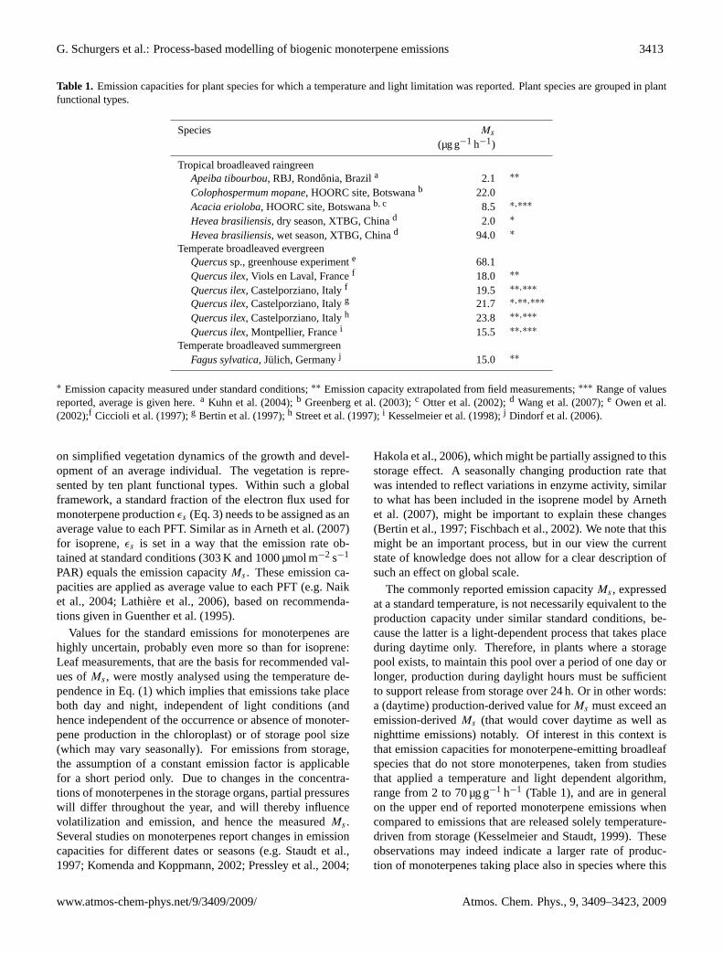
Table 1. Emission capacities for plant species for which a temperature and light limitation was reported. Plant species are grouped in plantfunctional types.
∗ Emission capacity measured under standard conditions;∗∗ Emission capacity extrapolated from field measurements;∗∗∗ Range of valuesreported, average is given here.a Kuhn et al. (2004);b Greenberg et al. (2003);c Otter et al. (2002);d Wang et al. (2007);e Owen et al.(2002);f Ciccioli et al. (1997);g Bertin et al. (1997);h Street et al. (1997);i Kesselmeier et al. (1998);j Dindorf et al. (2006).
on simplified vegetation dynamics of the growth and devel-opment of an average individual. The vegetation is repre-sented by ten plant functional types. Within such a globalframework, a standard fraction of the electron flux used formonoterpene productionεs (Eq. 3) needs to be assigned as anaverage value to each PFT. Similar as in Arneth et al. (2007)for isoprene,εs is set in a way that the emission rate ob-tained at standard conditions (303 K and 1000 µmol m−2 s−1
PAR) equals the emission capacityMs . These emission ca-pacities are applied as average value to each PFT (e.g. Naiket al., 2004; Lathiere et al., 2006), based on recommenda-tions given in Guenther et al. (1995).
Values for the standard emissions for monoterpenes arehighly uncertain, probably even more so than for isoprene:Leaf measurements, that are the basis for recommended val-ues ofMs , were mostly analysed using the temperature de-pendence in Eq. (1) which implies that emissions take placeboth day and night, independent of light conditions (andhence independent of the occurrence or absence of monoter-pene production in the chloroplast) or of storage pool size(which may vary seasonally). For emissions from storage,the assumption of a constant emission factor is applicablefor a short period only. Due to changes in the concentra-tions of monoterpenes in the storage organs, partial pressureswill differ throughout the year, and will thereby influencevolatilization and emission, and hence the measuredMs .Several studies on monoterpenes report changes in emissioncapacities for different dates or seasons (e.g. Staudt et al.,1997; Komenda and Koppmann, 2002; Pressley et al., 2004;
Hakola et al., 2006), which might be partially assigned to thisstorage effect. A seasonally changing production rate thatwas intended to reflect variations in enzyme activity, similarto what has been included in the isoprene model by Arnethet al. (2007), might be important to explain these changes(Bertin et al., 1997; Fischbach et al., 2002). We note that thismight be an important process, but in our view the currentstate of knowledge does not allow for a clear description ofsuch an effect on global scale.
The commonly reported emission capacityMs , expressedat a standard temperature, is not necessarily equivalent to theproduction capacity under similar standard conditions, be-cause the latter is a light-dependent process that takes placeduring daytime only. Therefore, in plants where a storagepool exists, to maintain this pool over a period of one day orlonger, production during daylight hours must be sufficientto support release from storage over 24 h. Or in other words:a (daytime) production-derived value forMs must exceed anemission-derivedMs (that would cover daytime as well asnighttime emissions) notably. Of interest in this context isthat emission capacities for monoterpene-emitting broadleafspecies that do not store monoterpenes, taken from studiesthat applied a temperature and light dependent algorithm,range from 2 to 70 µg g−1 h−1 (Table 1), and are in generalon the upper end of reported monoterpene emissions whencompared to emissions that are released solely temperature-driven from storage (Kesselmeier and Staudt, 1999). Theseobservations may indeed indicate a larger rate of produc-tion of monoterpenes taking place also in species where this
3414 G. Schurgers et al.: Process-based modelling of biogenic monoterpene emissions
Table 2. Presence or absence of long-term monoterpene storage organs (+ indicates monoterpene storing PFT,− indicates non-storing), andemission capacities for the plant functional types used for the global simulation as adopted from Naik et al. (2004).
production rate cannot be observed directly, because of thestorage acting as a buffer between production and emission.
In the model, leaf production of monoterpenes is similarfor all plants, independent of presence or absence of storage.For the application of storage (Eq. 4) the produced monoter-penes can be transferred into storage, depending on the plantfunctional type (PFT). To do so, the group of PFTs was sepa-rated as in Table 2: all broadleaved trees are considered to benon-storing, while the conifers and herbs are considered tobe storing monoterpenes. Such a simplification is unavoid-able in DGVMs and is based on current observations: anisoprene-like release of monoterpenes was mostly found inbroadleaved species, whereas conifers tend to have monoter-pene storage (Kesselmeier and Staudt, 1999). Large amountof stored monoterpenes are also observed in many herbaciousspecies.
Two global simulations were performed using the vege-tation dynamics of LPJ-GUESS in DVGM mode, applyingboth the short-term temperature-dependent algorithm, andthe production and storage algorithm. The CRU climate datafor the years 1901–2000 were used to force the model witha spinup of 300 years, using the atmospheric CO2 concen-tration for 1901 (290 ppm) and a detrended series of datafor 1901–1950. This was followed by 100 years of sim-ulation representing the 20th century, using the CRU dataand CO2 concentrations from ice cores and from observa-tions. Simulations were performed at a horizontal resolu-tion of 0.5◦
×0.5◦, the average of the last 20 years of this run(1981–2000) was used for the analysis. The effects of the twodifferent algorithms on global monoterpene emissions werecompared. For both simulations, the emission capacities asin Naik et al. (2004) were adopted (Table 2). The first simula-tion assumes all monoterpenes to be released with the short-term temperature algorithm (Eq. 1), changes in the amountof monoterpene storage are not considered. This assumptionalso underlies all global scale estimates to date (see overview
in Arneth et al., 2008a). The second simulation calculatesproduction of monoterpenes from electron transport (Eq. 2).Monoterpenes are emitted either directly, or from a storagepool (conifers and herbs, Eq. 5). For this simulation, emis-sion capacitiesMs (and thus the values ofεs) are adjustedas described above with a factor 2 to reflect the differencebetween the production (taking place only during sunlighthours) and the need to refill the storage (with emissions tak-ing place the entire day).
3 Results and discussion
3.1 Simulated monoterpene emissions
A prerequisite for reliable simulation of BVOC fluxes withvegetation models is the reproduction of important growthcharacteristics. For the Blodgett Forest site, simulated LAI(one-sided) was 2.6 for 2003 and 2.8 for 2004 (not shown),which compares well to the observed variation of 2 to 3 forthe study period (Holzinger et al., 2006). Simulated grossprimary productivity (GPP, Fig. 1b) also agreed well withobservations (Misson et al., 2006), except for a short periodin late July 2003, for which the simulated daily GPP wasapproximately reduced by 25% compared to the values de-rived from eddy flux data, likely due to an overestimationof drought stress in the model during that period. Measure-ments from other years indicate that Blodgett Forest experi-ences drought stress during summer, but the extent is lessthan in other Ponderosa pine forests with comparable cli-matic circumstances (Panek, 2004; Misson et al., 2004).
Simulations were performed with two different algorithmsfor monoterpene emissions: (1) using the temperature-dependent algorithm (Eq. 1), and (2) using the monoterpeneproduction algorithm (Eq. 2) for direct release (no storage)and for release from storage with time constants up to 160 d.The emission capacitiesMs that gave the best fit with each
G. Schurgers et al.: Process-based modelling of biogenic monoterpene emissions 3415
1 Jun 1 Jul 1 Aug 1 Sep 1 Oct 1 Nov 1 Dec 1 Jan 1 Feb 1 Mar0
5
10g
ross
ph
ot.
(g
C m
-2 d
-1)
simulationobservations
1 Jun 1 Jul 1 Aug 1 Sep 1 Oct 1 Nov 1 Dec 1 Jan 1 Feb 1 Mar051015202530
pre
cip
itat
ion
(m
m d
-1)
1 Jun 1 Jul 1 Aug 1 Sep 1 Oct 1 Nov 1 Dec 1 Jan 1 Feb 1 Mar
0
0.5
1
1.5
2
mo
no
terp
ene
flu
x (m
g C
m-2
d-1
)
temperature-dependent
photosynthesis-dependent
photosynthesis- and storage-dependent
observations
1 Jun 1 Jul 1 Aug 1 Sep 1 Oct 1 Nov 1 Dec 1 Jan 1 Feb 1 Mar-505
1015202530
tem
per
atu
re (
oC
)
1 Jun 1 Jul 1 Aug 1 Sep 1 Oct 1 Nov 1 Dec 1 Jan 1 Feb 1 Mar
date
0
50
100
150
200
250
mo
no
t. c
on
c. (
µg C
g-1
DW
)
(c)
(b)
(a)
(d)
Fig. 1. (a) Observed daily average air temperature (in red) and precipitation (in blue) forBlodgett forest; (b) Simulated and measured photosynthesis rates for Blodgett forest, Cali-fornia, for 2003; (c) Simulated monoterpene emissions with the temperature-dependent andphotosynthesis-dependent algorithms, applying storage of half of the production with τs = 80d, and observations for June 2003 - April 2004; (d) Simulated monoterpene storage in leavesfor the simulation with half the production stored applying τs = 80 d. Emission capacities in (c)were adjusted to match the average of the measured rates (see text).
34
Fig. 1. (a) Observed daily average air temperature (in red) and precipitation (in blue) for Blodgett Forest;(b) Simulated and measured(2003) photosynthesis rates for Blodgett Forest, California;(c) Simulated monoterpene emissions with the temperature-dependent andphotosynthesis-dependent algorithms, applying storage of half of the production withτs=80 d, and observations for June 2003–April 2004;(d) Simulated monoterpene storage in leaves for the simulation with half the production stored applyingτs=80 d. Emission capacities in (c)were adjusted to match the average of the measured rates (see text).
of the two algorithms (Eq. 1 and Eqs. 2–6 with various stor-age settings) are of the same order of magnitude (Table 3).Holzinger et al. (2006) report an emission capacity (usingEq. 1 and based on all-sided leaf area) of 1 µmol m−2 leafh−1 (or 0.20 µg C g−1 h−1), about half of the optimised valuefor Eq. (1) in this study. Differences between the two stud-ies could be caused by a difference in extrapolation from leaflevel to canopy level, as well as by the applied leaf tempera-ture correction in this study.
The simulated seasonality in emissions (Fig. 1c, for clar-ity only a selection of the simulations summarized in Table 3is displayed) was very similar in all simulations, irrespec-tive of the presence or absence of storage. This is due tothe fact that temperature is always a main contributor to thevariability since temperature and radiation normally corre-late well, and warm days also have large rates of electronflux and hence monoterpene production. Only at high val-ues forτs (≥40 d) the seasonal differences were considerablyreduced (not shown). Without storage, the photosynthesis-dependent simulated emissions show a strong day-to-dayvariability, as was the case with GPP (Fig. 1b), due to the de-
pendence of terpene production on photosynthetic processes.The observed monoterpene emission peaks due to rain events(Fig. 1a and c) as were observed before at the same site(Schade et al., 1999) were not captured by any of the simula-tion experiments. These peaks in emissions are likely causedby enhanced humidity of the air and a related uptake of wa-ter by the leaves (Llusia and Penuelas, 1999; Schade et al.,1999). Simulated changes in seasonality are caused only bychanges in weather conditions and changes in the size of thestorage pool, we did not include an explicit change of sea-sonality of monoterpene production as is often suggested forisoprene production in relation to changes in isoprene syn-thase activity (Wiberley et al., 2005).
Simulations performed with the photosynthesis-dependentalgorithm (Eq. 2) combined with release from storage ofmonoterpenes (Eq. 5) showed an interesting feature: Thebest agreement between the fitted parameterization and ob-servations, determined from the average mean error (AME)and the root mean square error (RMSE) between the two,was obtained both with no storage at all and with high resi-dence times in storage (τs=80 d, Table 3). However, the ratio
3416 G. Schurgers et al.: Process-based modelling of biogenic monoterpene emissions
Table 3. Results from simulations for Blodgett Forest: scaled emission capacityMs , average mean error (AME), root mean square error(RMSE), ratio between summer (JJA) and winter (DJF) emissions for all days (for days with observation available in brackets,n=38 forsummer,n=18 for winter).
Simulation Ms AME RMSE MsumMwin
µg C g−1 h−1 mg C m−2 d−1 mg C m−2 d−1
Temperature-dependent 0.41 0.154 0.047 4.1 (3.5)
Photosynthesis-dependent 0.42 0.189 0.063 22.1 (13.6)Photosynthesis- and storage-dependentτs=2.5 d 0.42 0.197 0.069 22.0 (16.3)Photosynthesis- and storage-dependentτs=5 d 0.42 0.194 0.065 18.1 (15.2)Photosynthesis- and storage-dependentτs=10 d 0.41 0.191 0.064 11.0 (10.2)Photosynthesis- and storage-dependentτs=20 d 0.41 0.189 0.064 5.9 (5.6)Photosynthesis- and storage-dependentτs=40 d 0.43 0.185 0.063 3.7 (3.4)Photosynthesis- and storage-dependentτs=80 d 0.45 0.185 0.063 2.7 (2.6)Photosynthesis- and storage-dependentτs=160 d 0.50 0.258 0.108 1.3 (1.3)
Photosynthesis- and storage-dependent half stored,τs=80 d 0.44 0.158 0.049 5.7 (5.0)
between simulated summer and winter emissions decreaseswith increasing residence times due to the delay caused bythe storage. The observed summer to winter emissions ra-tio of 5.3 was reproduced in the simulations only at valuesfor τs≥40 d. Although observations for important parts ofthe simulation period were absent, the reasonably good fitswith both low(τs=0 d) and high(τs=80 d) residence times,combined with the need for long storage to fit the ratio be-tween summer and winter emissions, merits the assumptionthat part of the produced monoterpenes might be emitted di-rectly, whereas another part is stored for considerable times.Such a mixture of long-term storage and direct emission (oremission from short-term storage, which is ignored in thisstudy) was suggested by Staudt et al. (1997, 2000) forPi-nus pinea, and was proposed in a more general manner byKesselmeier and Staudt (1999). A simulation which tookthis assumption into account (half of the produced monoter-penes was simulated to be emitted directly, the other half wasstored with a standard residence timeτs of 80 d) resulted inlower values for both AME and RMSE, with values close tothose obtained with the short-term temperature-dependent al-gorithm, and in a ratio of summer and winter emissions closeto the observed value (5.0 based on the days for which ob-servations were available). Increasing the standardized res-idence timeτs caused the concentration of monoterpenes inthe leaves to increase to values up to 300 µg C g−1 at aτs of160 d (not shown), and the maximum concentration to be de-layed until later in the year compared to the simulations withsmallerτs . Storage also caused the day-to-day variability ofemissions to decrease (Fig. 1c), acting as a buffer betweenproduction and emission, as is the case for non-specific stor-age (Niinemets et al., 2004). Observed concentrations ofβ-pinene in a Ponderosa pine forest in Oregon, US, ranged be-tween 2.8×10³ and 5.1×10³ µg C g−1 (Lerdau et al., 1994)
for September and June, respectively, with emission rates of0.2 and 1.1 µg C g−1 h−1, which indicates a similar order ofmagnitude for the residence times as obtained in our simula-tions.
The simulated seasonality of monoterpene concentrationsin the Ponderosa pine plantation for the applied split of theemissions in storage (half) and direct emissions (half) isshown in Fig. 1d. The peak in simulated leaf monoterpeneconcentrations was reached in autumn. For the range oftime coefficients applied (Table 3), the peak in concentrationsshifted from summer(τs=2.5 d) to late autumn(τs=160 d),and the concentrations increased with increasingτs (notshown). Measurements of the seasonal cycle of monoterpeneconcentrations in other species show a wide variety of pat-terns: A pattern similar to the simulated one, with high con-centrations in summer and autumn, was observed for Blackspruce (Picea mariana) in Canada (Lerdau et al., 1997), butnot so for Jack pine (Pinus banksiana) in Canada, whereconcentrations peaked in spring and autumn (Lerdau et al.,1997). Measurements of terpene concentrations in severalMediterranean species indicated low concentrations in sum-mer and high in winter due to higher emissions at high tem-peratures (Llusia et al., 2006).
Our results did not account for changes in leaf mass overthe year, which would affect the maximum storage pool sizeand could account for some of the variation observed in thetiming of peak values and emissions. However, there arelikely other factors playing an important role in the timingof emissions that are not considered in our vegetation model.For instance, Back et al. (2005) were able to reproduce largespring emissions of monoterpenes in borealPinus sylvestrisby incorporating photorespiration as a carbon source, al-though the link between terpenoid production and photores-piration is controversial (Hewitt et al., 1990; Penuelas and
G. Schurgers et al.: Process-based modelling of biogenic monoterpene emissions 3417
Llusia, 2002). It is also plausible that terpene synthesis couldtake place during winter, since conifers are able to assim-ilate, albeit at low rates, during warm winter periods (e.g.Suni et al., 2003).
3.2 Sensitivity to changes in temperature and light
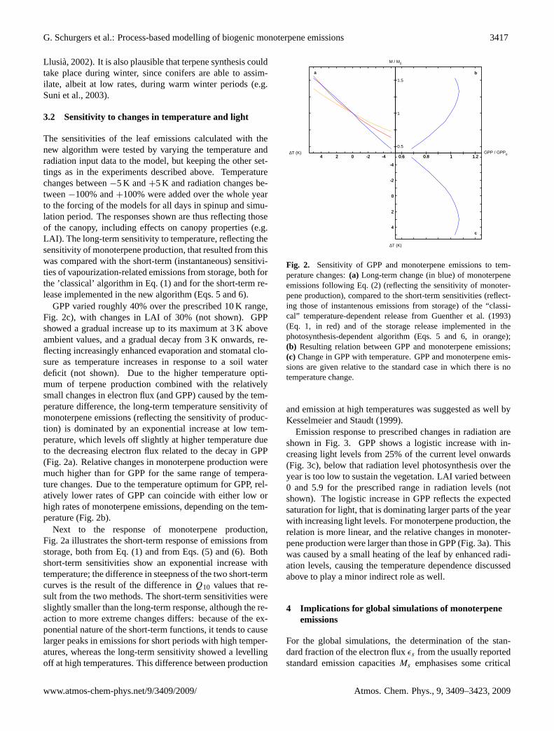
The sensitivities of the leaf emissions calculated with thenew algorithm were tested by varying the temperature andradiation input data to the model, but keeping the other set-tings as in the experiments described above. Temperaturechanges between−5 K and+5 K and radiation changes be-tween−100% and+100% were added over the whole yearto the forcing of the models for all days in spinup and simu-lation period. The responses shown are thus reflecting thoseof the canopy, including effects on canopy properties (e.g.LAI). The long-term sensitivity to temperature, reflecting thesensitivity of monoterpene production, that resulted from thiswas compared with the short-term (instantaneous) sensitivi-ties of vapourization-related emissions from storage, both forthe ’classical’ algorithm in Eq. (1) and for the short-term re-lease implemented in the new algorithm (Eqs. 5 and 6).
GPP varied roughly 40% over the prescribed 10 K range,Fig. 2c), with changes in LAI of 30% (not shown). GPPshowed a gradual increase up to its maximum at 3 K aboveambient values, and a gradual decay from 3 K onwards, re-flecting increasingly enhanced evaporation and stomatal clo-sure as temperature increases in response to a soil waterdeficit (not shown). Due to the higher temperature opti-mum of terpene production combined with the relativelysmall changes in electron flux (and GPP) caused by the tem-perature difference, the long-term temperature sensitivity ofmonoterpene emissions (reflecting the sensitivity of produc-tion) is dominated by an exponential increase at low tem-perature, which levels off slightly at higher temperature dueto the decreasing electron flux related to the decay in GPP(Fig. 2a). Relative changes in monoterpene production weremuch higher than for GPP for the same range of tempera-ture changes. Due to the temperature optimum for GPP, rel-atively lower rates of GPP can coincide with either low orhigh rates of monoterpene emissions, depending on the tem-perature (Fig. 2b).
Next to the response of monoterpene production,Fig. 2a illustrates the short-term response of emissions fromstorage, both from Eq. (1) and from Eqs. (5) and (6). Bothshort-term sensitivities show an exponential increase withtemperature; the difference in steepness of the two short-termcurves is the result of the difference inQ10 values that re-sult from the two methods. The short-term sensitivities wereslightly smaller than the long-term response, although the re-action to more extreme changes differs: because of the ex-ponential nature of the short-term functions, it tends to causelarger peaks in emissions for short periods with high temper-atures, whereas the long-term sensitivity showed a levellingoff at high temperatures. This difference between production
-4-2024∆T (K)
0.5
1
1.5
-4-2024 0.6 0.8 1 1.2GPP / GPP0
M / M0
0.6 0.8 1 1.2
-4
-2
0
2
4
∆T (K)
-4
-2
0
2
4
a b
c
Fig. 2. Sensitivity of GPP and monoterpene emissions to temperature changes: (a) Long-termchange (in blue) of monoterpene emissions following equation 2 (reflecting the sensitivity ofmonoterpene production), compared to the short-term sensitivities (reflecting those of instante-nous emissions from storage) of the ’classical’ temperature-dependent release from Guentheret al. (1993) (equation 1, in red) and of the storage release implemented in the photosynthesis-dependent algorithm (equations 5 and 6, in orange); (c) Change in GPP with temperature; (b)Resulting relation between GPP and monoterpene emissions. GPP and monoterpene emis-sions are given relative to the standard case in which there is no temperature change.
35
Fig. 2. Sensitivity of GPP and monoterpene emissions to tem-perature changes:(a) Long-term change (in blue) of monoterpeneemissions following Eq. (2) (reflecting the sensitivity of monoter-pene production), compared to the short-term sensitivities (reflect-ing those of instantenous emissions from storage) of the “classi-cal” temperature-dependent release from Guenther et al. (1993)(Eq. 1, in red) and of the storage release implemented in thephotosynthesis-dependent algorithm (Eqs. 5 and 6, in orange);(b) Resulting relation between GPP and monoterpene emissions;(c) Change in GPP with temperature. GPP and monoterpene emis-sions are given relative to the standard case in which there is notemperature change.
and emission at high temperatures was suggested as well byKesselmeier and Staudt (1999).
Emission response to prescribed changes in radiation areshown in Fig. 3. GPP shows a logistic increase with in-creasing light levels from 25% of the current level onwards(Fig. 3c), below that radiation level photosynthesis over theyear is too low to sustain the vegetation. LAI varied between0 and 5.9 for the prescribed range in radiation levels (notshown). The logistic increase in GPP reflects the expectedsaturation for light, that is dominating larger parts of the yearwith increasing light levels. For monoterpene production, therelation is more linear, and the relative changes in monoter-pene production were larger than those in GPP (Fig. 3a). Thiswas caused by a small heating of the leaf by enhanced radi-ation levels, causing the temperature dependence discussedabove to play a minor indirect role as well.
4 Implications for global simulations of monoterpeneemissions
For the global simulations, the determination of the stan-dard fraction of the electron fluxεs from the usually reportedstandard emission capacitiesMs emphasises some critical
3418 G. Schurgers et al.: Process-based modelling of biogenic monoterpene emissions
00.511.52Q / Q0
0
0.5
1
1.5
2
2.5
3
00.511.52 0 0.5 1 1.5 2 2.5GPP / GPP0
M / M0
0 0.5 1 1.5 2 2.50
0.5
1
1.5
2
Q / Q0
0
0.5
1
1.5
2
a b
c
Fig. 3. Sensitivity of GPP and monoterpene emissions to changes in radiation: (a) Change inmonoterpene emissions with light; (c) Change in GPP with light; (b) Resulting relation betweenGPP and monoterpene emissions. Radiation level, GPP and monoterpene emissions are givenrelative to the standard case in which there is no radiation change.
36
Fig. 3. Sensitivity of GPP and monoterpene emissions to changesin radiation: (a) Change in monoterpene emissions with light;(b) Resulting relation between GPP and monoterpene emissions;(c) Change in GPP with light. Radiation level, GPP and monoter-pene emissions are given relative to the standard case in which thereis no radiation change.
uncertainties in understanding the processes that determineseasonal and annual emission patterns. The difference be-tween an emission-based and a production-based value ofMs , as discussed in Sect. 2.4, was estimated to be approxi-mately a factor of two, which reflects the difference betweendaylight hours and 24 h as well as the additional light limita-tion of the production and thus emissions. Incidentally, mea-sured emission capacities of broadleaved trees where emis-sions are light-dependent, and the standardized rates hencerepresent the monoterpene production, also tend to be sub-stantial (Table 1), supporting the view that the leaf produc-tion of monoterpenes during daylight hours is larger thanseen when emissions are measured from storage pool release.Ms was therefore doubled compared to the simulations usingEq. (1).
Annual global total terrestrial emissions were29.6 Tg C a−1 for the simulation that assumed monoter-penes to be uniformly emitted from storage (Eq. 1), and31.8 Tg C a−1 for the simulation that was based on pro-duction and storage, and that accounted for the frequentlyobserved emissions without storage in broadleaved veg-etation (Eq. 2). The spatial distribution of the emissionsis surprisingly similar in the two cases (Fig. 4). Theproduction and storage algorithm resulted in larger rates intemperate forest regions in the eastern US, southern Braziland China. In these areas, the applied correction factor oftwo is apparently too large compared to the actual reductionby the light dependence. In dry regions in subtropicalAfrica, Northern India and Australia, where temperaturesare high but photosynthesis rates are relatively low, the
Fig. 4. (a) Global monoterpene emissions (mg C m−2 a−1) as simulated with the temperature-dependent short-term emission algorithm (Eq. 1), and (b) global monoterpene emissions assimulated with the new photosynthesis-dependent algorithm (Eq. 2). Shown are averages for1981–2000.
37
Fig. 4. (a)Global monoterpene emissions ( mg C m−2 a−1) as sim-ulated with the temperature-dependent short-term emission algo-rithm (Eq. 1), and(b) global monoterpene emissions as simulatedwith the new photosynthesis-dependent algorithm (Eq. 2). Shownare averages for 1981–2000.
temperature-dependent algorithm resulted in larger rates.Our estimates of global annual monoterpene emissions are
at the low end of the published global totals. Naik et al.(2004), using the temperature dependence (Guenther et al.,1995) algorithm, reported 33 Tg C a−1, which is comparableto our estimate with the same algorithm. These two exper-iments are comparable in their experimental design as well:both use potential natural vegetation cover, with similar treePFTs in both models while Naik et al. (2004) simulated twoadditional shrub PFTs. However, these estimates are a factorof four lower than the highest published estimates (Guen-ther et al., 1995 report 127 Tg C a−1, Lathiere et al., 2006report 117 Tg C a−1). This emphasises the large uncertaintyin global BVOC emission calculations that can be introducedthrough use of different basal rates, vegetation cover and phe-nology, climatology, temporal resolution, and the use of dif-ferent algorithms (Arneth et al., 2008a).
For the global simulations, storage was applied for theconiferous and herbaceous plant functional types (Table 2),with half of the produced monoterpenes being stored, ap-plying a standard residence timeτs of 80 d. In the ab-sence of of long-term changes in the storage pool size, theparameterization of the storage equations (Eqs. 5 and 6)affects only the the seasonality of the emissions, but notthe annual totals. However, the seasonality of emissionsis an important feature of monoterpene emission simulationwhen it comes to linking these to atmospheric chemistry.
G. Schurgers et al.: Process-based modelling of biogenic monoterpene emissions 3419
Application of monoterpene storage in the model with theparameters as derived in the local simulations caused signif-icant residence times (averaged for all PFTs) mainly at highlatitudes (Fig. 5). Large latitudinal differences between sim-ulations with and without storage occur in spring and autumnat high latitudes. During spring, when environmental con-ditions allow the onset of photosynthesis and monoterpeneproduction, the storage pool is being built up, thereby mov-ing part of the production into this storage pool and reduc-ing the emitted amount. Moving from pole to equator, thedifference between the simulations with and without storageis diminishing due to higher temperatures and the relativelylarger contribution of directly emitting PFTs (Table 2).
5 Conclusions
We present here an analysis of monoterpene emissions thatseeks to investigate the effects of two important processesseparately, namely the production in the chloroplast and theensuing emissions that may or may not be from a storagepool. The analysis aims to provide a basis for better un-derstanding of observed seasonal patterns as well as to takeinto account the increasing evidence of a direct, production-driven emission pattern in broadleaved vegetation.
The short-term sensitivities to temperature changes forboth algorithms were comparable, but also the short-termsensitivity (on volatilization) and the long-term sensitivity(on production) were shown to be remarkably similar, at leastas long as small changes in temperature are considered. Wedid not focus here on how the different monoterpene emis-sion algorithms would be affected in simulations that takeinto account future climate change. It would seem that al-gorithms that include solely a response to increasing tem-perature would be more sensitive under future warming sce-narios compared to those that also include a light-limitation,but the overall effects of climate change on other importantprocesses like changes in leaf area index or vegetation coverwould also need to be considered. What is more, it is un-certain whether the response of monoterpene production toincreasing atmospheric CO2 concentration follows a similarinhibitory pattern as is shown for isoprene in an increasingnumber of plants (Constable et al., 1999; Loreto et al., 2001;Staudt et al., 2001; Baraldi et al., 2004), although the simi-larity in the chloroplastic pathways would suggest a similarresponse.
It is a general problem of BVOC emission modelling thatparameterizations of algorithms that seek to represent ob-served constraints on emissions can only be based on a verylimited number of studies and that true process understand-ing is often lacking (Guenther et al., 2006; Arneth et al.,2008a). Accounting in a global model for entire plant func-tional types to have either similar storage residence time orrelease monoterpenes directly is an inevitable necessity, but itcannot do justice to the natural variation. While most conif-
Fig. 5. Annual cycle of the average residence time (in days) of the monoterpenes in the storagepool, shown are zonal means for the period 1981-2000. All PFTs (including the non-storingPFTs) are weighted according to their leaf area index in order to calculate latitudinal averages.
38
Fig. 5. Annual cycle of the average residence time (in days) ofthe monoterpenes in the storage pool, shown are zonal means forthe period 1981–2000. All PFTs (including the non-storing PFTs)are weighted according to their leaf area index in order to calculatelatitudinal averages.
erous species that have been studied to date release monoter-penes mostly from storage, there are nonetheless species thatemit part of their monoterpenes light-dependently (e.g.Pi-nus pinea, Staudt et al., 1997, 2000). At the same time,some broadleaf monoterpene emitters may also include stor-age organs (e.g. emissions fromEucalyptusspp. have beenshown to depend primarily on temperatures, He et al., 2000).New DGVM model developments that – at least on conti-nental scale – are capable of representing actual tree speciesdistribution, rather than PFTs, can be used to assess the un-certainties associated with these globally applied simplifiedassumptions (e.g. Arneth et al., 2008b). Such a distinc-tion would also allow for a more detailed description of thedifferent types of monoterpenes that are emitted. Currentemission inventories do account for a plant species-specificfractionation of different monoterpenes (e.g. Steinbrecheret al., 2009). However, a temporal variation in the compo-sition of monoterpenes, as observed (Staudt et al., 2000) hasnot been accounted for so far. Additionally, the distinctionbetween monoterpene-storing and non-monoterpene-storingplant functional types has the potential to be extended tomonoterpene types that are stored or non-stored. For in-stance, inPinus pineaseveral studies (Staudt et al., 1997,2000) have shown a clear distinction between monoterpenesthat are stored and thus have mainly temperature-dependentemission (e.g. limonene,α-pinene), and monoterpenes withemissions that react more directly in response to diurnal pat-terns of light or to shading, and that do not exhibit long-termstorage (e.g. trans-β-ocimene, 1,8-cineole). Such a distinc-tion does not only influence the diurnal course of emissions,
3420 G. Schurgers et al.: Process-based modelling of biogenic monoterpene emissions
but affects the annual course as well (Staudt et al., 2000).Eventually, such a model setup could also provide the ba-sis for describing emissions that can occur in response tophysical damage (e.g. by wind, rain or herbivores, Banchioet al., 2005; Pichersky et al., 2006). Such an analysis wouldpresent an important step forward on regional scale whenseasonal emission rates are used in atmospheric chemistrysimulations.
Acknowledgements.This research was supported by grants fromVetenskapsradet and the European Commission via a Marie CurieExcellence grant. We thank Laurent Misson for providing GPPdata from Blodgett Forest, Jaana Back,Ulo Niinemets, Russ Mon-son and Jorg-Peter Schnitzler for discussions on monoterpeneemissions and storage, and Marion Martin for comments on themanuscript. Extensive comments from two anonymous reviewershelped to improve the manuscript considerably.
Edited by: J. Rinne
References
Arneth, A., Niinemets, U., Pressley, S., Back, J., Hari, P., Karl, T.,Noe, S., Prentice, I., Serca, D., Hickler, T., Wolf, A., andSmith, B.: Process-based estimates of terrestrial ecosystem iso-prene emissions: incorporating the effects of a direct CO2-isoprene interaction, Atmos. Chem. Phys., 7, 31–53, 2007,http://www.atmos-chem-phys.net/7/31/2007/.
Arneth, A., Monson, R., Schurgers, G., Niinemets, U., andPalmer, P.: Why are estimates of global isoprene emissionsso similar (and why is this not so for monoterpenes)?, Atmos.Chem. Phys., 8, 4605–4620, 2008a,http://www.atmos-chem-phys.net/8/4605/2008/.
Arneth, A., Schurgers, G., Hickler, T., and Miller, P.: Effects ofspecies composition, land surface cover, CO2 concentration andclimate on isoprene emissions from European forests, Plant Bi-ology, 10, 150–162, doi:10.1055/s-2007-965247, 2008b.
Aumont, B., Madronich, S., Bey, I., and Tyndall, G. S.: Contri-bution of secondary VOC to the composition of aqueous atmo-spheric particles: a modeling approach, J. Atmos. Chem., 35,59–75, doi:10.1023/A:1006243509840, 2000.
Back, J., Hari, P., Hakola, H., Juurola, E., and Kulmala, M.: Dy-namics of monoterpene emissions inPinus sylvestrisduring earlyspring, Boreal Environ. Res., 10, 409–424, 2005.
Banchio, E., Zygadlo, Y., and Valladares, G. R.: Effects of me-chanical wounding on essential oil composition and emission ofvolatiles fromMinthostachys mollis, J. Chem. Ecol., 31, 719–727, 2005.
Baraldi, R., Rapparini, F., Oechel, W., Hastings, S., Bryant, P.,Cheng, Y., and Miglietta, F.: Monoterpene emission responsesto elevated CO2 in a Mediterranean-type ecosystem, New Phy-tol., 161, 1–21, 2004.
Bertin, N., Staudt, M., Hansen, U., Seufert, G., Ciccioli, P., Fos-ter, P., Fugit, J. L., and Torres, L.: Diurnal and seasonal courseof monoterpene emissions fromQuercus ilex(L.) under naturalconditions application of light and temperature algorithms, At-mos. Environ., 31, 135–144, 1997.
Chung, S. H. and Seinfeld, J. H.: Global distribution and climateforcing of carbonaceous aerosols, J. Geophys. Res., 107, 4407,doi:10.1029/2001JD001397, 2002.
Ciccioli, P., Fabozzi, C., Brancaleoni, E., Cecinato, A., Frattoni, M.,Loreto, F., Kesselmeier, J., Schafer, L., Bode, K., Torres, L.,and Fugit, J.-L.: Use of the isoprene algorithm for predictingmonoterpene emission from the Mediterranean holm oakQuer-cus ilexL.: Performance and limits of this approach, J. Geophys.Res., 102, 23319–23328, 1997.
Constable, J., Litvak, M., Greenberg, J., and Monson, R.: Monoter-pene emission from coniferous trees in response to elevated CO2concentration and climate warming, Glob. Change Biol., 5, 255–267, 1999.
Dement, W., Tyson, B., and Mooney, H.: Mechanism of monoter-pene volatilization inSalvia mellifera, Phytochemistry, 14,2555–2557, 1975.
Dindorf, T., Kuhn, U., Ganzeveld, L., Schebeske, G., Ciccioli, P.,Holzke, C., Koble, R., Seufert, G., and Kesselmeier, J.: Sig-nificant light and temperature dependent monoterpene emissionsfrom European beech (Fagus sylvaticaL.) and their potential im-pact on the European volitile organic compound budget, J. Geo-phys. Res., 111, D16305, doi:10.1029/2005JD006751, 2006.
Dudareva, N., Pichersky, E., and Gershenzon, J.: Biochemistry ofplant volatiles, Plant Physiol., 135, 1893–1902, 2004.
Farquhar, G., Von Caemmerer, S., and Berry, J.: A biochemi-cal model of photosynthetic CO2 assimilation in leaves of C3species, Planta, 149, 78–90, 1980.
Fischbach, R., Staudt, M., Zimmer, I., Rambal, S., and Schnit-zler, J.-P.: Seasonal pattern of monoterpene synthase activitiesin leaves of the evergreen treeQuercus ilex, Physiol. Plantarum,114, 354–360, 2002.
Franceschi, V. R., Krokene, P., Christiansen, E., and Krekling, T.:Anatomical and chemical defenses of conifer bark againstbark beetles and other pests, New Phytol., 167, 353–376,doi:10.1111/j.1469-8137.2005.01436.x, 2005.
Gershenzon, J., Maffei, M., and Croteau, R.: Biochemical and his-tochemical localization of monoterpene biosynthesis in the glan-dular trichomes of spearmint (Mentha spicata), Plant Physiol.,89, 1351–1357, 1989.
Gershenzon, J., Murtagh, G., and Croteau, R.: Absence of rapid ter-pene turnover in several diverse species of terpene-accumulatingplants, Oecologia, 96, 583–592, 1993.
Gershenzon, J., McConkey, M., and Croteau, R.: Regulation ofmonoterpene accumulation in leaves of Peppermint, Plant Phys-iol., 122, 205–213, 2000.
Greenberg, J., Guenther, A., Harley, P., Otter, L., Veenen-daal, E., Hewitt, C., James, A., and Owen, S.: Eddy fluxand leaf-level measurements of biogenic VOC emissions frommopane woodland of Botswana, J. Geophys. Res., 108, 8466,doi:10.1029/2002JD002317, 2003.
Grote, R., Mayrhofer, S., Fischbach, R., Steinbrecher, R.,Staudt, M., and Schnitzler, J.-P.: Process-based modelling of iso-prenoid emissions from evergreen leaves ofQuercus ilex(L.),Atmos. Environ., 40, S152–S165, 2006.
Guenther, A., Zimmerman, P., Harley, P., Monson, R., and Fall, R.:Isoprene and monoterpene emission rate variability: model eval-uations and sensitivity analyses, J. Geophys. Res., 98, 12609–12617, 1993.
Guenther, A., Hewitt, C., Erickson, D., Fall, R., Geron, C.,
G. Schurgers et al.: Process-based modelling of biogenic monoterpene emissions 3421
Graedel, T., Harley, P., Klinger, L., Lerdau, M., McKay, W.,Pierce, T., Scholes, B., Steinbrecher, R., Tallamraju, R., Tay-lor, J., and Zimmerman, P.: A global model of natural volatileorganic compound emissions, J. Geophys. Res., 100, 8873–8892,1995.
Guenther, A., Karl, T., Harley, P., Wiedinmyer, C., Palmer, P., andGeron, C.: Estimates of global terrestrial isoprene emissions us-ing MEGAN (Model of emissions of gases and aerosols fromnature), Atmos. Chem. Phys., 6, 3181–3210, 2006,http://www.atmos-chem-phys.net/6/3181/2006/.
Hakola, H., Tarvainen, V., Back, J., Ranta, H., Bonn, B., Rinne, J.,and Kulmala, M.: Seasonal variation of mono- and sesquiterpeneemission rates of Scots pine, Biogeosciences, 3, 93–101, 2006,http://www.biogeosciences.net/3/93/2006/.
Haxeltine, A. and Prentice, I.: A general model for the light-use ef-ficiency of primary production, Funct. Ecol., 10, 551–561, 1996.
He, C., Murray, F., and Lyons, T.: Seasonal variations in monoter-pene emissions fromEucalyptusspecies, Chemosphere, 2, 65–76, doi:10.1016/S1465-9972(99)00052-5, 2000.
Hewitt, C., Monson, R., and Fall, R.: Isoprene emissions from thegrassArundo donaxL. are not linked to photorespiration, PlantSci., 66, 139–144, 1990.
Hickler, T., Smith, B., Sykes, M., Davis, M., Sugita, S., andWalker, K.: Using a generalized vegetation model to simulatevegetation dynamics in Northeastern USA, Ecology, 85, 519–530, 2004.
Hoffmann, T., Odum, J. R., Bowman, F., Collins, D., Klockow, D.,Flagan, R. C., and Seinfeld, J. H.: Formation of organic aerosolsfrom the oxidation of biogenic hydrocarbons, J. Atmos. Chem.,26, 189–222, 1997.
Holzinger, R., Lee, A., McKay, M., and Goldstein, A. H.: Seasonalvariability of monoterpene emission factors for a Ponderosa pineplantation in California, Atmos. Chem. Phys., 6, 1267–1274,2006, http://www.atmos-chem-phys.net/6/1267/2006/.
Jenkin, M. and Clemitshaw, K.: Ozone and other secondary photo-chemical pollutants: chemical processes governing their forma-tion in the planetary boundary layer, Atmos. Environ., 34, 2499–2527, 2000.
Kesselmeier, J. and Staudt, M.: Biogenic volatile organic com-pounds (VOC): an overview on emission, physiology and ecol-ogy, J. Atmos. Chem., 33, 23–88, 1999.
Kesselmeier, J., Bode, K., Schafer, L., Schebeske, G., Wolf, A.,Brancaleoni, E., Cecinato, A., Ciccioli, P., Frattoni, M., Du-taur, L., Fugit, J. L., Simon, V., and Torres, L.: Simultaneousfield measurements of terpene and isoprene emissions from twodominant mediterranean oak species in relation to a North Amer-ican species, Atmos. Environ., 32, 1947–1953, 1998.
Komenda, M. and Koppmann, R.: Monoterpene emis-sions from Scots pinePinus sylvestris: field studies ofemission rate variabilities, J. Geophys. Res., 107, 4161,doi:10.1029/2001JD000691, 2002.
Kuhn, U., Rottenberger, S., Biesenthal, T., Wolf, A., Schebeske, G.,Ciccioli, P., Brancaleoni, E., Frattoni, M., Tavares, T.,and Kesselmeier, J.: Seasonal differences in isoprene andlight-dependent monoterpene emission by Amazonian treespecies, Glob. Change Biol., 10, 663–682, doi:10.1111/j.1529-8817.2003.00771.x, 2004.
Lathiere, J., Hauglustaine, D., De Noblet-Ducoudre, N., Krin-ner, G., and Folberth, G.: Past and future changes in biogenic
volatile organic compound emissions simulated with a globaldynamic vegetation model, Geophys. Res. Lett., 32, L20818,doi:10.1029/2005GL024164, 2005.
Lathiere, J., Hauglustaine, D., Friend, A., De Noblet-Ducoudre, N.,Viovy, N., and Folberth, G.: Impact of climate variability andland use changes on global biogenic volatile organic compoundemissions, Atmos. Chem. Phys., 6, 2129–2146, 2006,http://www.atmos-chem-phys.net/6/2129/2006/.
Lerdau, M., Dilts, S., Westberg, H., Lamb, B., and Allwine, E.:Monoterpene emission from ponderosa pine, J. Geophys. Res.,99, 16609–16015, 1994.
Lerdau, M., Matson, P., Fall, R., and Monson, R.: Ecological con-trols over monoterpene emissions from Douglas-fir (Pseudot-suga menziesii), Ecology, 76, 2640–2647, 1995.
Lerdau, M., Litvak, M., Palmer, P., and Monson, R.: Controls overmonoterpene emissions from boreal forest conifers, Tree Phys-iol., 17, 563–569, 1997.
Lichtenthaler, H., Rohmer, M., and Schwender, J.: Two indepen-dent biochemical pathways for isopentenyl diphosphate and iso-prenoid biosynthesis in higher plants, Physiol. Plantarum, 101,643–652, 1997.
Litvak, M. and Monson, R.: Patterns of induced and constitutivemonoterpene production in conifer needles in relation to insectherbivory, Oecologia, 114, 531–540, 1998.
Llusia, J. and Penuelas, J.:Pinus halepensisandQuercus ilexter-pene emission as affected by temperature and humidity, Biol.Plantarum, 42, 317–320, 1999.
Llusia, J., Penuelas, J., Alessio, G. A., and Estiarte, M.: Seasonalcontrasting changes of foliar concentrations of terpenes and othervolatile organic compound in four domiant species of a Mediter-ranean shrubland submitted to a field experimental drought andwarming, Physiol. Plantarum, 127, 632–649, 2006.
Loreto, F., Ciccioli, P., Cecinato, A., Brancaleoni, E., Frattoni, M.,Fabozzi, C., and Tricoli, D.: Evidence of the photosynthetic ori-gin of monoterpenes emitted byQuercus ilexL leaves by C-13labeling, Plant Physiol., 110, 1317–1322, 1996.
Loreto, F., Fischbach, R., Schnitzler, J.-P., Ciccioli, P., Brancale-oni, E., Calfapietra, C., and Seufert, G.: Monoterpene emissionand monoterpene synthase activities in the Mediterranean ever-green oakQuercus ilexL. grown at elevated CO2 concentrations,Glob. Change Biol., 7, 709–717, 2001.
Loreto, F., Pinelli, P., Manes, F., and Kollist, H.: Impact of ozoneon monoterpene emissions and evidence for an isoprene-like an-tioxidant action of monoterpenes emitted byQuercus ilex, TreePhysiol., 24, 361–367, 2004.
McConkey, M. E., Gershenzon, J., and Croteau, R. B.: Develop-mental regulation of monoterpene biosynthesis in the glandulartrichomes of peppermint, Plant Physiol., 122, 215–223, 2000.
Mihaliak, C., Gershenzon, J., and Croteau, R.: Lack of rapidmonoterpene turnover in rooted plants: implications for theoriesof plant chemical defense, Oecologia, 87, 373–376, 1991.
Misson, L., Panek, J., and Goldstein, A. H.: A comparison of threeapproaches to modeling leaf gas exchange in annually drought-stressed ponderosa pine forests, Tree Physiol., 24, 529–541,2004.
Misson, L., Tang, J. W., Xu, M., McKay, M., and Goldstein, A. H.:Influences of recovery from clear-cut, climate variability, andthinning on the carbon balance of a young ponderosa pine plan-tation, Agr. Forest Meteorol., 130, 207–222, 2005.
3422 G. Schurgers et al.: Process-based modelling of biogenic monoterpene emissions
Misson, L., Gershenson, A., Tang, J., McKay, M., Cheng, W., andGoldstein, A. H.: Influences of canopy photosynthesis and sum-mer rain pulses on root dynamics and soil respiration in a youngponderosa pine forest, Tree Physiol., 26, 833–844, 2006.
Mitchell, T. D. and Jones, P. D.: An improved method of construct-ing a database of monthly climate observations and associatedhigh-resolution grids, Int. J. Climatol., 25, 693–712, 2005.
Naik, V., Delire, C., and Wuebbles, D.: Sensitivity ofglobal biogenic isoprenoid emissions to climate variabil-ity and atmospheric CO2, J. Geophys. Res., 109, D06301,doi:10.1029/2002JD003203, 2004.
New, M., Hulme, M., and Jones, P.: Representing twentieth-centuryspace-time climate variability. Part II: Development of 1901-96monthly grids of terrestrial surface climate, J. Climate, 13, 2217–2238, 2000.
Niinemets, U. and Reichstein, M.: A model analysis of the ef-fects of nonspecific monoterpenoid storage in leaf tissues onemission kinetics and composition in Mediterranean sclero-phyllous Quercusspecies, Global Biogeochem. Cy., 16, 1110,doi:10.1029/2002GB001927, 2002.
Niinemets, U., Seufert, G., Steinbrecher, R., and Tenhunen, J.:A model coupling foliar monoterpene emissions to leaf pho-tosynthetic characteristics in Mediterranean evergreenQuercusspecies, New Phytol., 153, 257–275, 2002.
Otter, L., Guenther, A., Wiedinmyer, C., Fleming, G.,Harley, P., and Greenberg, J.: Spatial and temporal varia-tions in biogenic volatile organic compound emissions forAfrica south of the equator, J. Geophys. Res., 108, 8505,doi:10.1029/2002JD002609, 2003.
Otter, L. B., Guenther, A., and Greenberg, J.: Seasonal and spa-tial variations in biogenic hydrocarbon emissions from southernAfrican savannas and woodlands, Atmos. Environ., 36, 4265–4275, 2002.
Owen, S., Harley, P., Guenther, A., and Hewitt, C.: Light depen-dency of VOC emissions from selected Mediterranean plants,Atmos. Environ., 36, 3147–3159, 2002.
Panek, J.: Ozone uptake, water loss and carbon exchange dynamicsin annually drought-stressedPinus ponderosaforests: measuredtrends and parameters for uptake modeling, Tree Physiol., 24,277–290, 2004.
Penuelas, J. and Llusia, J.: Linking photorespiration, monoterpenesand thermotolerance inQuercus, New Phytol., 155, 227–237,doi:10.1046/j.1469-8137.2002.00457.x, 2002.
Pichersky, E., Noel, J. P., and Dudareva, N.: Biosynthesis of plantvolatiles: nature’s diversity and ingenuity, Science, 311, 808–811, 2006.
Pressley, S., Lamb, B., Westberg, H., Guenther, A., Chen, J., andAllwine, E.: Monoterpene emissions from a Pacific Northwestold-growth forest and impact on regional biogenic VOC emissionestimates, Atmos. Environ., 38, 3089–3098, 2004.
Ruuskanen, T. M., Kolari, P., Back, J., Kulmala, M., Rinne, J.,Hakola, H., Taipale, R., Raivonen, M., Altimir, N., and Hari, P.:On-line field measurements of monoterpene emissions fromScots pine by proton-transfer-reaction mass spectrometry, BorealEnviron. Res., 10, 553–567, 2005.
Schade, G., Goldstein, A. H., and Lamanna, M.: Are monoter-
pene emissions influenced by humidity?, Geophys. Res. Lett.,26, 2187–2190, 1999.
Schuh, G., Heiden, A. C., Hoffmann, T., Kahl, J., Rockel, P.,Rudolph, J., and Wildt, J.: Emissions of volatile organic com-pounds from sunflower and beech: dependence on temperatureand light intensity, J. Atmos. Chem., 27, 291–318, 1997.
Simpson, D., Yttri, K. E., Klimont, Z., Kupiainen, K., Caseiro, A.,Gelencser, A., Pio, C., Puxbaum, H., and Legrand, M.: Modelingcarbonaceous aerosol over Europe: analysis of the CARBOSOLand EMEP EC/OC campaigns, J. Geophys. Res.-Atmos., 112,D23S14, doi:10.1029/2006JD008158, 2007.
Sitch, S., Smith, B., Prentice, I., Arneth, A., Bondeau, A.,Cramer, W., Kaplan, J., Levis, S., Lucht, W., Sykes, M., Thon-icke, K., and Venevsky, S.: Evaluation of ecosystem dynamics,plant geography and terrestrial carbon cycling in the LPJ Dy-namic Global Vegetation Model, Glob. Change Biol., 9, 161–185, 2003.
Smith, B., Prentice, I., and Sykes, M.: Representation of vegetationdynamics in the modelling of terrestrial ecosystems: compar-ing two contrasting approaches within European climate space,Global Ecol. Biogeogr., 10, 621–637, 2001.
Staudt, M. and Bertin, N.: Light and temperature dependence ofthe emission of cyclic and acyclic monoterpenes from holm oak(Quercus ilexL.) leaves, Plant Cell Environ., 21, 385–395, 1998.
Staudt, M. and Seufert, G.: Light-dependent emission of monoter-penes by Holm Oak (Quercus ilexL.), Naturwissenschaften, 82,89–92, 1995.
Staudt, M., Bertin, N., Hansen, U., Seufert, G., Ciccioli, P., Fos-ter, P., Frenzel, B., and Fugit, J.-L.: Seasonal and diurnal patternsof monoterpene emissions fromPinus pinea(L.) under field con-ditions, Atmos. Environ., 31, 145–156, 1997.
Staudt, M., Bertin, N., Frenzel, B., and Seufert, G.: Seasonal vari-ation in amount and composition of monoterpenes emitted byyoungPinus pineatrees – implications for emission modeling, J.Atmos. Chem., 35, 77–99, 2000.
Staudt, M., Joffre, R., Rambal, S., and Kesselmeier, J.: Effect ofelevated CO2 on monoterpene emission of youngQuercus ilextrees and its relation to structural and ecophysiological parame-ters, Tree Physiol., 21, 437–445, 2001.
Steinbrecher, R., Smiatek, G., Koble, R., Seufert, G., Theloke, J.,Hauff, K., Ciccioli, P., Vautard, R., and Curci, G.: Intra- andinter-annual variability of VOC emissions from natural and semi-natural vegetation in Europe and neighbouring countries, Atmos.Environ., 43, 1380–1391, doi:10.1016/j.atmosenv.2008.09.072,2009.
Street, R., Owen, S., Duckham, S., Boissard, C., and Hewitt, C.: Ef-fect of habitat and age on variations in volatile organic compound(VOC) emissions fromQuercus ilexandPinus pinea, Atmos. En-viron., 31, 89–100, 1997.
Suni, T., Berninger, F., Vesala, T., Markkanen, T., Hari, P.,Makela, A., Ilvesniemi, H., Hanninen, H., Nikinmaa, E., Hut-tula, T., Laurila, T., Aurela, M., Grelle, A., Lindroth, A., Ar-neth, A., Shibistova, O., and Lloyd, J.: Air temperature triggersthe recovery of evergreen boreal forest photosynthesis in spring,Glob. Change Biol., 9, 1410–1426, 2003.
Tingey, D., Manning, M., Grothaus, L., and Burns, W.: Influence oflight and temperature on monoterpene emission rates from Slashpine, Plant Physiol., 65, 797–801, 1980.
Tsigaridis, K. and Kanakidou, M.: Global modelling of secondary
G. Schurgers et al.: Process-based modelling of biogenic monoterpene emissions 3423
organic aerosol in the troposphere: a sensitivity analysis, Atmos.Chem. Phys., 3, 1849–1869, 2003,http://www.atmos-chem-phys.net/3/1849/2003/.
Turner, G. W., Gershenzon, J., and Croteau, R. B.: Development ofpeltate glandular trichomes of peppermint, Plant Physiol., 124,665–679, 2000.
Wang, Y.-F., Owen, S. M., Li, Q.-J., and Penuelas, J.: Monoterpeneemissions from rubber trees (Hevea brasiliensis) in a changinglandscape and climate: chemical speciation and environmentalcontrol, Glob. Change Biol., 13, 2270–2282, doi:10.1111/j.1365-2486.2007.01441.x, 2007.
Wiberley, A., Linskey, A., Falbel, T., and Sharkey, T.: Developmentof the capacity for isoprene emission in kudzu, Plant Cell Envi-ron., 28, 898–905, 2005.
Yokouchi, Y., Hijikata, A., and Ambe, Y.: Seasonal variation ofmonoterpene emission rate in a pine forest, Chemosphere, 13,255–259, 1984.