Process Dynamics and Control · 2007-03-05 · Process Dynamics and Control - Digital Control -...

<Lecture Note>

Process Dynamics and Control

- Digital Control -

Korea University

Dept. of Chem. Eng.

Dae Ryook Yang

Department of Chemical Engineering, Korea UniversityDigital Process Control 1

Host

Computer

Front-end

Computer

Front-end

Computer

Interface Interface

Process Process

Part Six : Digital Control Technique

Chap 21. Digital Computer Control

Microprocessor

Analog Controller -------------> Digital Computer Control

Economically justifiable nowadays!

⇒ Choice of correct system - single/multiple computer, microprocessor based

system, ...

* Role for digital computer system in Process Control

Passive application : Data acquisition (manipulation of process data)

Active application : Manipulation of the process by computer

<Distributed data processing>

Complex calculationSupervisory control

Data acquisition

A/D, D/A, Transmitter,....amplifier...

4-20mA, 1-5V, 3-15psig

Process + sensor & actuator

Sensor Transmitter ADC DAC Transmitter Actuator

0-100℃

5-200psig

0-50gpm

. . .

4-20mA

1-5V

0-10V

0.04mV/℃

12bit

(0-4095)

16bit, . . .

→ →

→ Computer →

→ →

4-20mA

1-5V

0-10V

+ Hold

mA

1-5V

0-10V

Valve opening

Inverter output

Displacement


Chap 22. Sampling and Filtering of continuous Measurement

For data acquisition and control with computer based system, Specify

1. Sampling rate

2. S/N ratio, signal conditioning

3. control law

22.1. Sampling and Signal Reconstruction

Sampling Period : Δt (min)

Sampling Rate : f s=1Δt

(cycle / min)

Sampling freq. : ws=2πΔt

(rad / min)

Continuous Signal Sampled Signal

y( t) ----------→ y*(t)

Sampler

* Impulse modulation : representation of sampled signal

digital signal ------------→ continuous signal Signal Reconstruction by DAC + Hold


Zero-order hold : yH= yn-1 for t n-1≤ t < t n

Ho(s)=1-e

- sΔt

s

<disadvantages of ZOH>

1. ZOH starts attenuating at freq.'s considerably below ws

2. ZOH allows high freq.'s to pass although they are attenuated.

3. ZOH provides apparent time delay of one half of sampling period

H(s) =1-e - sΔt

s

( s→jω)=>

H( jω) =2e - jωΔt/2(e j

ωΔt/2-e - jωΔt/2)2jω

=Δt sin(ωΔt/2)

ωΔt/2e - jωΔt/2

HG*(jω)=

1Δt ∑

∞

n=-∞H(jω+ jnω s)G( jω+ jnω s) ≅ e

- sΔt/2G(s)

First-order hold: yH = yn-1 + (t- t n-1

Δt) ( y n-1- y n-2) for t n-1≤ t < t n

H 1(s)=1+Δt s

Δt(1-e

- sΔt

s) 2

→ High order holds do not offer significant advantages for most control problem

→ ZOH is most widely used.

Fractional order Hold: yH = yn-1 + α(t- tn-1

Δt) ( y n-1- y n-2) for t n-1≤ t < t n

Continuous Slewing: yH = yn-2 + (t-tn-1

Δt) ( y n-1- y n-2) for t n-1≤ t < t n

Hc(s)=1Δt

(1-e

- sΔt

s) 2

<Block diagram of digital control system>

* Multirate sampling : use of different sampling period in the same system


22.2. Selection of the Sampling Period

Selection of Δt based on

1. # of measurement

2. view point of process control

<aliasing> --- foldover effect

Sampling rate must be large enough not to loose significant process

information

* Shannon's Sampling theorem :

- Sampling freq. must be more than twice the freq. of sine wave(original signal)

"To be able to recover the continuous signal from its sampled

counterpart, the sampling freq. (ωs) must be at least twice the

highest freq. (ωc) in the signal."

⇒ actual signal has all freq.

⇒ it is impossible to recover the continuous signal from its sampled counterpart.

Aliasing can happen for the sampling of nonsinusoidal signal.

⇒ Use anti-aliasing filter

<Selection of Sampling Period>

* S/N ratio = σ2s

σ2N

(σ2 : variance)

based on process variable type : Flow, level, temp...

based on open-loop system : τ, θ, τmax, settling time, ωc

⇒ Selection of sampling period is less significant nowadays!


22.3. Signal Processing and Data Filtering

Noise Sources : measurement device → filtering

electrical equipment → Shielding, grounding

process itself → filtering

(multiphase flow, mixing, turbulence, . . . )

filter = Transfer function !

<Analog filter>

τFdy(t)dt

+y( t)= x( t)

τF: Filter time constant, y( t) : filtered value, x( t) : measured value

- steady-state gain of the filter = 1

- exponential filter = Low pass filter = RC filter

- Before Sampling, use analog filter to reduced the noise

→ prefiltering → anti-aliasing filter

- if τF < 3 sec, use passive analog filter (R, C....)

if τF > 3 sec, use active analog filter (op amplifier)

- Usually τF < 0.1 τ

max

- τF should be selected so that (lowest noise freq. wN)

wN > wF=2πτF

> w max =2π

τmax

<Digital filters>

* Exponential filter

xn-1,xn..... : measured

yn-1,yn ..... : filtered

Use of backward difference approximation for analog filter

τF

y n-y n-1

Δt+ y n= x n


yn=Δt

τF+Δt

xn+τF

τF+Δt

yn-1

α=1

τF/Δt+1

: filter constant ⇒ τF=

Δt(1-α)α

yn=αxn+(1-α)yn-1 : Weighted summation!

⇒ single exponential smoothing

α=1 : No filtering ( τF=0), α=0 : measurement is ignored ( τ

F=∞),

<Double Exponential Filter>

----> Exp. filter ----> Exp. filter ---->

xn yn yn

yn=γyn+(1-γ) yn-1

yn=γαxn+γ(1-α) yn-1+(1-γ) yn-1

( yn-1=γyn-1+(1-γ) yn-2 => yn-1=1γ yn-1-

1-γγ yn-2

)

=γαxn+(2-γ-α) yn-1 - (1-α) (1-γ) yn-2

Simplification : γ=α

yn= α 2xn+2(1-α) yn-1-(1-α) 2 yn-2

⇒ better filtering for high freq. noise than exponential filter

<Moving average filter>

yn=1J ∑

n

i=n- J+1x i J: moving window size

yn-1=1J ∑

n-1

i=n-Jx i

yn= yn-1+1J

(xn-xn- J) (recursive form) : low pass filter


<Noise spike filter (rate of change filter)>

yn={xn if | xn-yn-1| ≤Δxyn-1-Δx if yn-1-xn >Δxyn-1+Δx if yn-1-xn <-Δx

(Δx : maximum change rate)

⇒ use for power glitch, instrument glitches, . . .

22.4. Comparison of Analog and Digital Filter

1. Digital filters can be easily tuned (programmed) to fit the process. They are also

easily modified.

2. Digital filters require the choice of sampling period

3. Digital filters affect the performance of computer system

4. Analog filters are particularly effective for elimination of high-frequency noise and

aliasing

22.5. Effect of filter selection on control system performance

filter → dynamic element → phase lag added → reduced stability limit

filter constant change → retune the controller!

To compensate the lag → D-mode in PID

Chap 23. Development of Discrete-Time Models

Discretize

Continuous-time model ------------> Discrete-time model

O.D.E difference eqn.

23.1 Finite Difference Model

dy( t)dt

= f(y,x) : y = output, x = input

by finite difference approximation (backward difference),


yn-yn-1

Δt≅ f (yn-1,xn-1) : Calculated from known quantities

⇒ yn=yn-1+ Δt f (yn-1,xn-1) : Recurrence relation

* It can be used for numerical integration (Euler integration)

Use of forward difference

dydt

≅yn+1-yn

Δt [shifting index : n→ (n-1)]

Interpolation formula : dydt

=y(k)+3y(k-1)-3y(k-2)-y(k-3)

6Δt

23.2 Exact Discretization of Linear Systems

For Linear D.E. and piecewise constant input (during the sampling period)

τ dy( t)dt

+y( t)= x( t) ; x( t)= x(0) (constant)y(0)≠0

Laplace Transform : sY(s)- y(0)=-1τ Y( s)+

1τx(0)s

Y(s)=1

s+1/τ[1τx(0)s

+ y (0)]

Inverse L. T. : y(t) =x(0)(1-e- t /τ

)+y(0) e- t /τ

∴ y(Δ t)=x(0) (1-e -Δ t/τ)+y(0) e -Δ t/τ

⋮

y(nΔt)= x ( (n-1)Δ t)(1-e -Δ t/τ)+y ( (n-1)Δ t)e -Δ t/τ

input (constant) initial condition

⇓

yn=e-Δ t/τ

yn-1+(1-e-Δ t/τ

)xn-1 ⇒ Exact Solution!

23.3 Higher-Order System

Linear Differential eq. of order p -> linear Difference eq. of order p

G(s)=Y(s)X(s)

=K(τ as+1)

(τ 1s+1)(τ 2s+1)


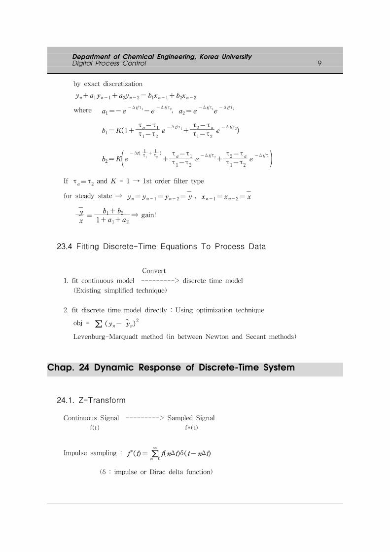
by exact discretization

yn+a 1yn-1+a 2yn-2=b 1xn-1+b 2xn-2

where a1=-e-Δ t/τ1-e

-Δ t/τ2, a2=e-Δ t/τ1e

-Δ t/τ2

b1=K(1+τa-τ

1

τ1-τ

2e

-Δ t/τ1+τ2-τ

a

τ1-τ

2e

-Δ t/τ2)

b2=K(e-Δt(

1τ1+

1τ2)

+τa-τ

1

τ1-τ

2e

-Δ t/τ2

+τ2-τ

a

τ1-τ

2e

-Δ t/τ1)If τ

a=τ2and K = 1 → 1st order filter type

for steady state ⇒ yn=yn-1=yn-2= y , xn-1=xn-2= x

y

x=

b 1+b 21+a 1+a 2

⇒ gain!

23.4 Fitting Discrete-Time Equations To Process Data

Convert

1. fit continuous model ---------> discrete time model

(Existing simplified technique)

2. fit discrete time model directly : Using optimization technique

obj = ∑ (yn- y n)2

Levenburg-Marquadt method (in between Newton and Secant methods)

Chap. 24 Dynamic Response of Discrete-Time System

24.1. Z-Transform

Continuous Signal ---------> Sampled Signal

f(t) f*(t)

Impulse sampling : f *(t)= ∑∞

n=0f(nΔt)δ( t-nΔt)

(δ : impulse or Dirac delta function)


( f(nΔt)=⌠⌡

nΔt+

nΔt-f*(t)dt)

ℒ[ f *(t) ]=F *(s)= ∑∞

n=0f(nΔt)e - nΔt s

e -nΔt s : real translation theorem for δ( t-nΔt)

Let z≜ e sΔt

F(z)≜ Z [ f * (t)]= ∑∞

n=0f(nΔt)z-n

≜ Z [ f( t)]

= Z [ f * (t)]= ∑∞

n=0fnz

-n

: Z-transform

⇒ Z-Transform is a special case of Laplace Transform

: Infinite series, but F(z) can be written in closed form if F( s) is a rational function

* Step function : S(t); f(nΔt) = 1 for all n ≥ 0 ( f 0 = 1 → f( 0+)=1)

F(z)=1+z-1

+z-2

+.......

For |z| > 1, F(z)=1

1-z-1

▶ |z| > 1 ↔ esΔt > 1 ⇒ s > 0 to have finite values!

* Exponential function : f( t)=Ce -at

F(z) = ∑∞

n=0Ce

- anΔtz

-n

if |e -anΔt z-1| < 1, F(z) =C

1-e - aΔt z-1

→ s > -a

(if a < 0, s should be s > -a >0 for e-ate-st to have limit if a<0)

Even for s <-a, the expression will be valid for all s using analytic extension theorem.


Properties of the Z-Transform

1. Linearity

Z [a 1f 1(t)+a 2f 2(t) ]= a 1Z [f 1(t)]+a 2Z [f 2(t)]

2. Real Translation Theorem

Z [ f( t- iΔt)]= z- i F(z) provided that f( t)=0 for t <0

pf)

Z [ f( t- iΔt)] = ∑∞

n=0f (nΔt- iΔt) z-n (Let j=n-i)

= ∑∞

j=- if( jΔt) z - j- i (f(j Δt)=0 for j< 0)

=z - i ∑∞

j=0f( jΔt) z (- j)=z- i F (z)

3. Complex Translation Theorem

Z[e - atf(t)]=F(ze aΔt)

pf)

Z [e - atf( t)] = ∑∞

n=0e - anΔtz-n

= ∑∞

i=0f(nΔt) (ze a

Δt) -n

=F(ze aΔt)

4. Initial Value Theorem

limn→0f(nΔt)= lim

z→∞(1-z-1)F(z) for |z| > 1

5. Final Value Theorem

limn→∞f(nΔt)= lim

z→1(1-z-1)F(z) for |z| > 1 provided f(∞Δt) exists.

pf)

limz→1

(1-z-1

)F(z)= limz→1

(1-z-1

) ∑∞

n=0f(nΔt)z- n

= limz→1

[f(0)+{ f(Δt)-f(0)}z-1+{ f(2Δt)-f(Δt)}z-2

+...}]


=[ f(0)+ f(Δt)- f(0)+ f(2Δt)- f(Δ t)+...+f(∞Δt)- f( (∞-1)Δt)]

= f(∞Δt)= limn→∞f(nΔt)

Ex 24.1 For f(t) = t, F(z) = ?

f(nΔt)=nΔt F(z) = ∑∞

n=0nΔtz -n

=Δt ∑∞

n=0nz

-n

Let S(z) = ∑∞

n=0nz -n,

S(z)-z -1S(z)= z -1+z -2+z -3+.......=1

1-z-1 -1

∴ S(z) =1

(1-z-1

)2 -

1

(1-z-1

)=

z -1

(1-z-1

)2

⇒ F(z) =ΔtS(z)=Δt z -1

(1-z -1) 2

Ex 24.2 Z( cosbt)=? Z(e - at cosbt)=?

Using Euler's identity, cos (nbΔt)= ½(e jnbΔt+e - jnb Δt) where j= -1

F(z) =Z( cosbt)= ∑∞

n=0( cosnbΔt)z-n

=12 ( ∑

∞

n= 0e jnb

Δtz - n+ ∑∞

n= 0e - jnb Δtz - n)

(Z-transformation for exponential functions)

=12 ( 1

1-e jbΔtz-1 +

1

1-e - jbΔtz-1 )

=12

2-2(ejbΔt

+e- jbΔt

2)z -1

1-2(e jb

Δt+e - jbΔt

2)z

-1+z

-2

=1-z -1 cos bΔt

1-2z-1

cos bΔt+z -2

(Note : if b= 2πnΔt

, then cos bΔt = 1 for t=Δt,2Δt.......nΔt

⇒ which results 1

1-z -1 : step function

⇒ fn=1 for all n → aliasing)

Using complex translation,

Z(e- at

cosbt) = F(zeaΔt

)

=1- z - 1e - a ΔtcosbΔt

1-2z- 1e

- a ΔtcosbΔt+ z - 2

e- 2a Δt


6. Modified Z-transform

(Special version of Z-transform for fractional time delays)

θ=(N+σ)Δt , 0<σ< 1, N is a positive integer

Z[f( t-θ)]= ∑∞

n=0f(nΔt-NΔt-σΔt)z-n

Let m=1-σ and k = n-N-1. Then,

Z[f( t-θ)]= ∑∞

k=-N-1f(kΔt+mΔt)z - k-N-1

since f(nΔt)=0 for n <0 → lower limit : k = 0

Z[f( t-θ)]= z-N-1∑∞

k=0f(kΔt+mΔt)z- k

∴ F(z,m)≜z -N-1∑∞

n=0f(kΔt+mΔt)z - k

* m : modified z-transform variable

⇒ Ogata has table for modified z-transform.

theorems for initial value, complex translation, etc are valid

⇒ it requires information between samples

-> Should know f(t)

Ex 24.3

F(z,m) =Zm(e-at) (N=0)

= z -1∑∞

n=0e -a (k+m)Δtz - k

=e -amΔtz -1∑∞

n=0e -akΔtz - k

=e-amΔt

z-1 1

1-e -aΔtz -1

For m=0 (σ=1), F(z,m) =z

-1

1-e - aΔtz -1

→ One unit time delay of e -at

Ex 24.4

F(s)=1

s( s+a) (a> 0); {= 1

a(1s-

1s+a

)}, limn→∞f (nΔt)=?


F(z)=1a(

1

1-z -1 -1

1-e -aΔtz -1 )

limn→∞f (nΔt) =

1a

limz→1

(1-z -1)(1

1-z -1 -1

1-e - aΔtz -1 )]

=1a

limz→1

[1-z-1

z-e- aΔt ]=

1a

24.2. Inversion of Z-Transform

F(z) -----------> f(t) Not unique

F(z) -----------> f *(t) or f *(nΔt)Unique

f *(t)=Z -1[F(z)]

F(z)=r 1

1-p 1z- 1 = r 1(1+ p 1z

- 1+ p 21z- 2+ .. . + pn1 z

- n)

⇒ f(nΔt)= f n= r 1 (p 1)n

Methods : a. Partial fraction expansion

b. Long Division

c. Contour integration

a) Partial fraction expansion

suppose F(z)=V 1(z)

V 2(z)

V 1 : kth order polynomial in z-1 excluding delay z-N

V 2 : mth order monic polynomial in z-1

(No positive power of z in numerator including delay)

F(z) =V 1(z)

(1-p 1z-1

)(1-p 2z-1

)....(1-pmz-1

)

=r 1

(1-p 1z-1)

+r 2

(1-p 2z-1)

+....+rm

(1-pmz-1)


Use of Heaviside's rule with z=1p i

⇒ f(nΔt)= z -1[r 1

(1-p 1z-1

)]+z -1[

r 2

(1-p 2z-1

)]+...+z -1[

rm

(1-pmz-1

)]

= r 1(p 1 )n+r 2(p 2 )

n+.......+rm(pm )

n (r i

(1-p iz-1

)⇒ r i p

ni)

* For simple case of f(nΔt)= r 1 p 1n

Stable region:

① → ② s= jω 0≤ω≤12

ωs

⇒ z=e jωΔt=1.0∡ωΔt, 0≤ω≤

12

ωs (half cycle)

∡0≤∡ωΔt ≤∡(12

ωsΔt) (ω s=2π/Δt) ⇒ 0∘≤ωΔt≤180∘(Upper half cycle)

Imaginary axis → unit circle

1st and 4th quadrant → outside the unit circle


2nd and 3rd quadrant → inside the unit circle

point (0,0) → point (1,0)

negative real axis → segment (0,1)

positive real axis → segment (1,∞)

Re(s) = -∞ → point (0,0)

Im(s) = ±½jωs with positive real→ segment (-1,-∞)

Im(s) = ±½jωs with negative real → segment (-1,0)

- If s= σ+ jω, z= e ( σ+ jω)Δt= eσΔt( cosωΔt+ jsinωΔt)

- For stability, σ≤0(ω≠0) in s-domain for all ω, it spans the inside of the unit circle

- If 0≤p i≤1, then

f(nΔt)= r 1e- q 1nΔt+r 2e

- q 2nΔt+. . .+rme- qmnΔt

where q i=-1Δt

lnp i

- If k>m (deg[V1(z)] > deg[V2(z)]), then partial fraction expansion is not strictly applicable

Ex. 24.5

Z-1[F(z)} = ? when F(z)=0.5z -1

(1-z -1)(1-0.5z -1) with Δt=1

Sol)

F(z) =r 1

1-z-1 +

r 2

1-0.5z-1

r 1=(1-z-1

)F(z)| z= 1=0.50.5

=1

r 2=(1-0.5z-1

)F(z)| z= 0.5=0.5*21-2

=-1

=1

1-z -1 -1

1-0.5z -1

where q 1=-1Δt

ln (1)=0, q 2=-1Δt

ln (0.5)=0.693

f(nΔt)=1-e-0.693nΔt

=1-(0.5)n


b) Long Division

F(z) = ∑∞

n=0f(nΔt)z - n

= f(0)+f(Δt)z -1+f(2Δt)z -2

+.........

F(z)=V 1(z)

V 2(z)=C 0+C 1z

-1+C 2z

-2+.......

Ex 24.6 Solve for Ex24.5 using long division.

0.5z-1+0.75z-2+0.875z-3+0.9375z-4+0.9687z-5+...┌────────────────────────────

1-1.5z-1+0.5z-2 │ 0.5z-1

→ Not in a closed form

c) Contour Integration

f(nΔt)=12πj

⌠⌡ΓF(z)z n-1dz

where Γ should be appropriately specified.

cf) For inverse Laplace transform, f( t)=12πj

limβ→∞

⌠⌡

α+ jβ

α- jβe stF(s)ds

- This method is seldom used in practice.

24.3. The Pulse Transfer Function

- Counterpart of Laplace domain "Transfer Function"

- input : x(nΔt) , X(z)

- output : y(nΔt) , Y(z)

- Convolution integral

y( t)=⌠⌡

t

0g(t-τ)x*(τ)dτ (g(t-τ) : impulse response)


where x *(τ)= ∑∞

k=0x(kΔt)δ(τ-kΔt)

y( t) =⌠⌡

t

0g(t-τ) ∑

∞

k=0x(kΔt)δ(τ-kΔt)dτ

= ∑∞

k=0g( t-kΔt)x(kΔt)

for t=nΔt,

y(nΔt) = ∑∞

k=0g(nΔt-kΔt)x(kΔt)

∴ Y(z) = ∑∞

n=0y(nΔt)z -n= ∑

∞

n=0∑∞

k=0g(nΔt-kΔt)x(kΔt)z -n

(Let i=n-k)

= ∑∞

i=-k∑∞

k=0g( iΔt)z -( i+ k)x(kΔt)

(g(iΔt) =0 for i<0)

= ∑

∞

i=0g( iΔt)z - i

∑∞

k=0x(kΔt)z- k

=G(z)X(z )

∴ G(z) ≜∑∞

i=0g( iΔt)z - i : Pulse Transfer function

Ex. 24.7

X(z)G(z) ?

Y(z)

if G(s)=k

τs+1

Sol)

g(t) =ℒ -1[G(s)]=kτ e

- t /τ

G(z) =kτ ∑

∞

n=0e -nΔt/τ z -n=

k/τ

1-e -Δ t/τz -1

Ex. 24.8 Find the Step response.

G(z)=-0.3225z -1+0.5712z -2

1-0.9744z-1

+0.2231z-2 ( = -0.3225z -1(1-1.771z -1)

(1+az-1

)(1+bz-1

) )


Sol) for unit step input X(Z)=1

1-z -1,

Y(z) =G(z)X(z)=G(z)1

1-z -1

by long division

= -0.3225z -1-0.0665z -2+0.2568z -3+0.5136z -4

+0.6918z -5+0.8082z -6+0.8820z -7+0.9277z -8

(First two coefficients have negative sign → inverse response)

Gain (z=1) = -0.3225+0.57121-0.9744+0.2231

=0.2487

0.0256+0.2231=1

24.4. Relating Pulse Transfer function to difference Equation

A general difference equation :

a 0yn+a 1yn-1+......+amy n-m=b 0xn+b 1x n-1+....bkxn- k

(From real translation theorem : Z[yn-i]=z-iY(z) )

Y(z)(a 0+a 1z-1

+a 2z-2

+...+amz-m

)=X(z)(b 0+b 1z-1

+b 2z-2

+...+bkz- k

)

G(z) =Y(z)X(z)

=b 0+b 1z

-1+b 2z-2....bkz

- k

a 0+a 1z-1

+a 2z-2

....amz-m

( b 0≠0 → immediate effect of input on output)

* Physical Realizability

From above eq'n, a0≠0 → physically realizable

(not depending on future inputs)

* The Zero-Order Hold (ZOH)

H(s)=1-e - sΔt

s


Ex. 24.10

G(s)=1

τs+1 : difference equation model for ZOH plus first-order process

Sol)

H(s)G(s) =1-e - sΔt

s1

τs+1

=( 1s -1

s+1/τ )-e - sΔt ( 1s-

1s+1/τ )

HG(z) =Z[H(s)G(s)]=Z{ℒ -1[H(s)G(s)]}

=(1

1-z -1 -1

1-e -Δ t/τz -1 )-z -1(1

1-z -1 -1

1-e -Δ t/τz -1 )

=z -1 (1-e -Δ t/τ)

1-e -Δ t/τz -1

Let a 1≜e-Δt/τ, Y(z)

X(z)=HG(z)=

(1-a 1)z-1

1-a 1z-1

⇒ yn-a 1yn-1=(1-a 1)x n-1

* HG(z)=Z[H(s)G(s)]= (1-z-1

) Z[G(s)s

]

HG(z)≠H(z)G(z)

(∵ H(z) =Z[1-e - sΔt

s]=(1-z -1)Z[

1s]=

1-z -1

1-z-1 =1 )

(1-z -1)Z[G(s)s

]≠Z [G(s)]

Ex. Prove limΔt→0HG(z)=G( s) for first orfer T.F.

limΔt→0HG(z)= lim

Δt→0

e- sΔt

( 1-e-Δ t/τ

)

1-e -Δ t/τe - sΔt = limΔt→0

-se- sΔt

+(s+1/τ)e ( s+1/τ)Δt

(s+1/τ) e ( s+1/τ)Δt

=-s+s+1/τ

s+1/τ=

1τs+1

=G(s)

c.f.) limΔt→0G(z)= lim

Δt→0

1/τ

1-e-Δ t /τ

e- sΔt =∞≠G(s)


Ex. 24.11

G( s)=Y(s)X( s)

=1s with ZOH → difference equation ?

Sol)

HG(z) =Z[H(s)G(s)]=Z[ (1-e -Δ t s)/s 2]=Δtz -1

1-z-1

( Z[1

s 2]=

Δtz -1

(1-z -1)2)

⇒ yn - yn-1 = Δt xn-1

by long division, yn=Δt ∑n

k=1xk-1

(integrating element)

* High-Order System

G( s)=Y( s)X( s)

=Ke -θ s

(τ 1s+1)(τ 2s+1) with ZOH and time delay(NΔt)

⇒ G(z) =(b 1+b 2z

-1)z -N-1

1+a 1z-1+a 2z

-2

⇒ apparent time delay is one sampling period longer.

24.5. Effect of Pole and Zero locations

- negative pole near unit circle has a pronounced effect

- ringing : alternation in sign of y

(Poles are easy)

- But the zero location is unpredictable, mainly due to sampling effect

⇒ No apparent simple relation

24.6. Conversion between Laplace and Z-Transform

- No ZOH is explicitly considered.

- Pade's approximation

z -1= e - sΔt≅2-sΔt2+sΔt

⇒ s≅2Δt

1-z -1

1+z -1

⇒ Tustin's method (bilinear transformation)


- Power Series expansion

z-1

= e- sΔt

=1-sΔt+s 2 Δt 2

2-.....

⇒ z-1

≅1-sΔt ⇒ s≅1-z -1

Δt (Backward difference formula)

- Approximate Z-Transform

s=1-z -1

Δt

s 2=z ( 1-z-1

Δt )2

s3=

2z

(1+z -1) ( 1-z -1

Δt )3

- Boxer-Thaler

s2=

12

(1+10z-1+z-2) (1-z-1

Δt )2

s3=

2z

(1+z -1) ( 1-z -1

Δt )3

Ex. 24.12

PID Controller : Gc(s)=Kc(1+1

τI s

+τD s) → obtain velocity form digital PID

Sol) Using s≅1-z -1

Δt

Gc(z)=Kc(a 0+a 1z

-1+a 2z

-2)

1-z -1

a 0= 1+ΔtτI+

τD

Δt

a 1=-(1+2τDτI

)

a 2=τD

Δt

let en : error, pn : output from the controller

Gc(z)=P(z)E(z)


(1-z -1)P(z) =Kc(a 0+a 1z-1+a 2z

-2)E(z)

= p n-p n-1=Δpn=Kca 0en+Kca 1e n-1+Kca 2e n-2

∴ Δpn=Kc[ (en-e n-1)+ΔtτIen+

τD

Δt(en-2e n-1+e n-2)]

* Tustin transformation will not give the same form.

Chap. 25 Analysis of Sampled Data Control System

- Block multiplication is different from Laplace transform case!

25.1 Open-Loop Block Diagram Analysis

- Synchronous sampling or process input / output

X*(s)= ∑

∞

n=0x(nΔt)e -nΔt s

X(z)= ∑∞

n=0x(nΔt)z -n

Y(s)=G( s)X*(s)

Y *(s)= [G( s)X *(s)]*=G *(s)X *(s)

[The Proof of this is in Franklin & Powell, p86, using freq.-domain analysis]

Y(z)=G(z)X(z)

* Pulse T.F. of Systems in Series

Y( s)=G 1(s)G 2(s)X*(s)

Y *(s)= [G 1 (s)G 2(s)]*X *(s)

Y(z)X(z)

=Z[G 1(s)G 2(s) ]=G 1G 2(z)

( G 1G 2(z)≠G 1(z)G 2(z) in general)


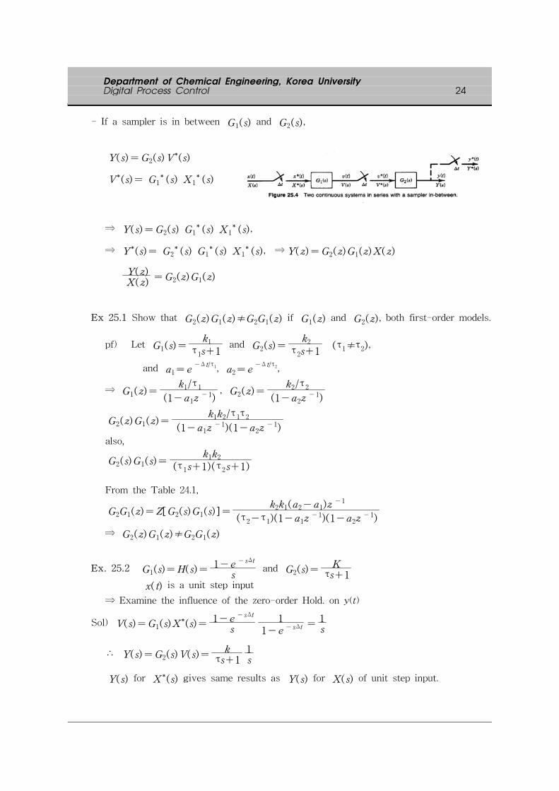
- If a sampler is in between G 1(s) and G 2(s),

Y( s)=G 2(s)V*(s)

V *(s)= G 1* (s) X 1

* (s)

⇒ Y( s)=G 2(s) G 1*(s) X 1

*(s),

⇒ Y *(s)= G 2* (s) G 1

* (s) X 1* (s), ⇒ Y(z)=G 2(z)G 1(z)X(z)

Y(z)X(z)

=G 2(z)G 1(z)

Ex 25.1 Show that G 2(z)G 1(z)≠G 2G 1(z) if G 1(z) and G 2(z), both first-order models.

pf) Let G 1(s)=k 1

τ1s+1

and G 2(s)=k 2

τ2s+1

(τ1≠τ2),

and a1=e-Δ t/τ1, a2=e

-Δ t/τ2,

⇒ G 1(z)=k 1/τ 1

(1-a 1z-1)

, G 2(z)=k 2/τ 2

(1-a 2z-1)

G 2(z)G 1(z)=k 1k 2/τ 1

τ2

(1-a 1z-1)(1-a 2z

-1)

also,

G 2(s)G 1(s)=k 1k 2

(τ 1s+1)(τ 2s+1)

From the Table 24.1,

G 2G 1(z)=Z[G 2(s)G 1(s) ]=k 2k 1(a 2-a 1)z

-1

(τ 2-τ1)(1-a 1z

-1)(1-a 2z-1)

⇒ G 2(z)G 1(z)≠G 2G 1(z)

Ex. 25.2 G 1(s)=H(s)=1-e - sΔt

s and G 2(s)=

Kτs+1

x( t) is a unit step input

⇒ Examine the influence of the zero-order Hold. on y(t)

Sol) V( s)=G 1(s)X*(s)=

1-e- sΔt

s1

1-e - sΔt =1s

∴ Y(s)=G 2(s)V( s)=k

τs+11s

Y(s) for X*(s) gives same results as Y(s) for X( s) of unit step input.


- For the case of sampling between G 1(s) and G 2(s)

Y( s) =G 2(s) G 1* (s)X *(s) = (

kτs+1

) (1-e - sΔt

s) * (

1s)*

=k

τs+1․1․(1+e - sΔt+e -2sΔt+......)

└→ (series of impulse input)

Ex. 25.3 G 1(s)=1s, G 2(s)=

12s+1

, X(s)=1s with ideal sampler ⇒ y( t)= ? for

0≤t≤6

(The last graph for y2 is wrong!)


y 1*(5)=5.91 y 2

*(5)=5.763

V(s) =G 1(s)X*(s)=

1s

1

1-e- sΔt V(s) =G 1(s)X

*(s)=1

( 1-e - sΔt )2

Y(s)=G 2(s)V(s)=1

s(2s+1)1

(1-e- sΔt

)Y(s) =G 2(s)V

*(s)=1

2s+11

(1-e - sΔt)2

=1

s(2s+1)(1+e - sΔt+e -2sΔt+.....) =

1(2s+1)

(1+e - sΔt+e -2sΔt+.....)2

=1

(2s+1)(1+2e - sΔt+3e -2sΔt+4e -2sΔt+...)

* Pulse Transfer Functions of Systems in Parallel

C( s) =C 1(s)+C 2(s)=G 1(s)E*(s)+G 2(s)E

*(s)

= [G 1(s)+G 2(s) ]E*(s)

⇒ C *(s)= [G*1(s)+G

*2(s) ]E

*(s)

⇒ C*(z)= [G 1(z)+G 2(z) ]E

*(z)

∴ C(z)E(z)

=G 1(z)+G 2(z)

- Case of continuous load change

C( s) =C 1(s)+C 2(s)=G 1(s)E*(s)+G 2(s)E( s)

C *(s) = G 1* (s)E *(s)+ [G 2 (s)E( s)]

*

C(z) =G 1(z)E(z)+G 2E(z)

⇒ No pulse transfer function.

25.2 Development of Closed-Loop Transfer Function


i) L(s)=0

B( s)=H( s)Gv(s)Gp(s)Gm(s)P*(s)

⇒ B *(s)= [HGvGpGm]*P *(s)

P*(s) = Gc

*(s)E

*(s)= Gc

*(s) [ R

*( s )-B

*(s)]

= Gc* (s) [ R *( s )- [HGvGpGm]

*P *(s)]

P*(s)=

Gc*(s) R( s )

1+ [HGvGpGm]* Gc

* (s)

C( s)=H( s)Gv(s)Gp(s)P*(s)

C *(s)= [HGvGp]*P *(s)

C*(s)=

[HGvGp]*Gc

*(s) R

*( s )

1+ [HGvGpGm]* Gc

* (s)

R *( s )=KmR*(s)

C*(s)

R *(s)=

[HGvGp]* Gc

* (s)Km

1+ [HGvGpGm]* Gc

* (s)

In Z-Transform notation,

C(z)R(z)

=KmHGvGp(z)Gc(z)

1+HGvGpGm(z)Gc(z)

The characteristic equation for the closed-loop control system,

1+HGvGpGm(z)Gc(z)=0 (determines stability)

If Gm(s)=Km,

C(z)R(z)

=HG(z)Gc(z)

1+HG(z)Gc(z), where HG(z)=HGvGpKm(z)

ii) R(s)=0

For simplicity, let Gm(s)=Km

{B( s)=H( s)Gv(s)Gp(s)KmP

*(s)+GL(s)KmL(s)

B *(s)=Km [HGvGp]*P *(s)+Km [GLL]

*

①


and

{C( s)=H( s)Gv(s)Gp(s)P

*(s)+GL(s)L( s)

C *(s)= [HGvGp]*P *(s)+ [GLL]

*

②

P *(s)=- Gc*B *(s) (∵ R(s) = 0) ③

① and ② → ③ and solve for P *(s)

C *(s)=GLL

*

1+KmHGv G p* (s) Gc

* (s)

C(z)=GLL(z)

1+Km H Gv Gp(z) Gc(z)=

GLL(z)

1+HG(z) Gc(z)

- Because the disturbance L(s) is not a sampled signal, closed-loop pulse T.F. cannot

be found.

- But the characteristic equations for set-point changes and load change are same

⇒ Same stability analysis.

Ex. 25.4 For previous block diagram,

Gp(s)=Kp e

-θS

τps+1

, GL(s)=KL

τLs+1

( τp=τ

L=τ)

Gc(z)=Kc, H(s)=1-e - sΔt

s, Gm=1, Gv=1

θ=NΔt and N is integer

⇒Find C(z) for load change and characteristic equation? ( R(s)=0, L( s)=1s)

Sol)

Z[GL(s)L( s)]=Z[KL

τLs+1

⋅1s]=Z[

KLs

-KLs+1/τ

]

=KL[1

1-z -1 -1

1-az -1 ]=KL(1-a)z

-1

(1-z -1)(1-az -1)

* Let a=e - Δt /τ

Z[H(s)Gp(s)]=Z[1-e - sΔt

s

Kpτs+1

e-θ s

]

=Z[ (e-NsΔt

-e-(N+1)sΔt

)1s⋅

kpτs+1

]


=Kp z-N(1-z -1)Z[

1s⋅

1τs+1

]

=Kp z-N(1-z -1)

(1-a)z -1

(1-z-1

)(1-az-1

)=Kp z

-N-1 (1-a)

(1-az-1

)

∴ C(z)=

KL(1-a)z-1

(1-z) (1-az-1

)

1+z -N-1KcKp(1-a)

1-az-1

=KL(1-a)z

-1

(1-z -1)(1-az -1+z -N-1KcKp(1-a))

=KL(1-a)z

-1

1-(1+a)z -1+az -2+KcKp(1-a)z-N-1-KcKp(1-a)z

-N-2

(Characteristic equation : the order of the equation depends on the time delay)

For Continuous System,

C(s)R( s)

=

Kp e-θ s

τs+1Kc

1+Kp e

-θ s

τs+1⋅Kc

=KcKp e

-θ s

τs+1+KpKc e-θ s

Characteristic equation : τ s+1+KcKp e-θ s=0

jτω+1+KcKpe- jθw

= jτw+1+KcKp( cos θω-jsin θω)=0

1+KcKpcos θω=0 and τω-KcKpsinθω=0

cosθω=-1KcKp

and sinθω=τω

KcKp

⇒ tanθω=-τω ⇒ infinite # of solution (periodic)

(while the discrete characteristic equation has limited # of roots.)

Ex 25.5 For Gc=Kc , Gp=Kp

τps+1

, Gm=Gv=1

What is limn→∞C(nΔt) for R(z) =

1

1-z -1?

sol) HG(z) =Kp(1-a)z

-1

1-az-1

( a=e-Δ t/τp)

C(z)R(z)

=

KcKp(1-a)z-1

1-az-1

1+KcKp(1-a)z

-1

1-az-1

=KcKp(1-a)z

-1

1+[Kc Kp(1-a)-a]z-1


for the stable pole, |z -1| > 1

|z|= |KcKp(1-a)-a| < 1

i) KcKp(1-a)< 1+a ⇒ KcKp<1+a1-a

ii) KcKp(1-a)>-(1-a) ⇒ KcKp>-1 (always satisfied due to negative

feedback)

* KcKp<1+a1-a

→ ∞ as a→1 ( Δt→0)

∴ if Δt→0, Kc can be infinite

(continuous system of 1st order + P-control does not cause stability problem for any Kc)

* KcKp<1+a1-a

→1 as a→0 ( Δt→∞)

For stable processes with a unit step input,

limz→1

(1-z -1)C(z)=KcKp(1-a)

1+KcKp(1-a)-a=

KcKpKcKp+1

As Kc→∞, C(z)→1 which follows R(z)! Otherwise, shows offset. ( C(z) <R(z)).

25.3 Stability of Sampled-Data Control System

* Definition : A linear sampled-data system is stable if the output sequence { y(nΔt)}

is bounded for any bounded input sequence { x(nΔt)}. Otherwise, the

system is said to be unstable. (BIBO stability)

⇒ No mention of the process response during the intersampled period (can be unstable

for continuous system)

It can be detected by changing sampling period or by using modified z-transform.

Asymptotically stable

Weakly stable

Bounded-input Bounded-state (BIBS) stable : stronger than the BIBO stable

Exponentially stable

Marginally stable


* The necessary and sufficient condition for stability of a linear sampled-data

system.

1) ∑∞

n=0|g(nΔt)| <∞ (non-decaying response will be excluded!) or,

2) G(z) has no poles on or outside the unit circle in z-plane.

* Stability Test

1. Modified Routh Stability Criterion

- The bilinear transformation z=1+w1-w

is not exact (z-plane to s-plane), but the

stability boundary is mapped exactly.

- Characteristic equation : Γ(z)=anzn+a n-1z

n-1+.....+a 1z+a 0=0

⇒ Γ(w)= anwn+ a n-1w

n-1+.....+ a 1w+ a 0=0

( a i = real constant, a i≠a i, generally)

Stability condition : ( an>0 w.l.o.g.)

i) a 0 ..... an are positive

ii) all elements in left column of Routh array are positive

⇒ # of sign change = # of unstable poles.

Ex 25.6

┌───────

Τ(z)=2z 3+z 2+z+1=0 │ 1 3

Τ(w)=2 (1+w1-w

)3

+ (1+w1-w

)2

+ (1+w1-w

)+1=0 │ 7 5

│ 16/7 0

⇒ w3+7w

2+3w+5=0 │ 5

⇒ Stable (all elements in the first column are positive)


<Jury Array>

a0 a1 . . . . . an

an an-1 . . . . . a0

b0 b1 . . . bn-1

bn-1 bn-2 . . . b1

⋮

r0 r1 r2 r3

r3 r2 r1 r0

s0 s1 s2

Total : (2n-3) rows

2. Jury's Stability Criteria

- Apply directly to polynomial in z (No # of unstable poles)

Stability Condition ( an >0, a i are real)

1) Γ(z=1)> 0

2) Γ(z=-1)> 0 for even n

Γ(z=-1)< 0 for odd n

3)

|a 0| <an|b 0|> |b n-1||c 0| > |c n-2|⋮|s 0| > |s 2|

(n-1) Constraints

where b k=| |a 0 an- kan ak

ck=| |b 0 bn- kbn b k

… s k=| |r 0 r 3- kr 3 r k

Ex 25.7 Γ(z)=2z4-3z

3+2z

2-z+1=0

i) & ii) Γ(1)=1> 0, Γ(-1)=9> 0 (n = 4, even)

iii) Jury array ① 1 -1 2 -3 2 ⇒ 1 < 2 (ok)

② 2 -3 2 -1 1

③-3 5 -2 -1 ⇒ 3 > 1 (ok)

④-1 -2 5 -3

⑤ 8 -17 11 ⇒ 8 ≯ 11 (violated)

⇒ Unstable

- If either first or last element is zero ⇒ Use special technique

3. Schur-Cohn Criteria

More complicated (About twice as many determinants must be calculated)

Ref. : Ogata. "Discrete-Time Control System", 1987


* Special Case of 0 element in the first column for Routh array

- 0 means a pair of imaginary roots

- replace 0 to ℇ, and proceed the calculation

- if above 0 and below 0 have sign change ⇒ consider as one sign change

s3 + 2s

2 + s + 2 = 0 s

5 + 2s

4 +24s

3 + 48s

2 - 25s - 50 = 0

┌──────── ┌────────

│ 1 1 │ 1 24 -25

│ 2 2 │ 2 48 -50 (→use as aux. polynomial)

│ 0 (→ replace with ℇ) │ 0 0

│ 2 ⇒ P(s) = 2s4 + 48s2 - 50

- if any derived row has all zero elements, use auxiliary polynomials,

⇒ two real roots with opposite sign radially and/or two conjugated imaginary roots

s5 + 2s

4 +24s

3 + 48s

2 - 25s - 50 = (s

2 - 1) (s

2 +25) (s + 2)

┌────────

│ 1 24 -25

│ 2 48 -50 ⇒ P(s) = 2s4 + 48s2 - 50

│ 8 96 ⇐ replace 0-row with dP/ds = 8s3 + 96s

│ 24 -50

│112.7 0

│-50

⇒ 4th order auxiliary polynomial (2 pairs of radially symmetric roots)

+ 1 sign change (one root with positive real)

⇒ a pair of conjugate imaginary roots

+ a pair of radially symmetric roots (one root with positive real)

⇒ Deg (Aux. Polynomial)/2 = no. of pairs of radially symmetric roots

(The order of auxiliary polynomial will always be even!)

* If s= z-σ ( σ= constant)

We can test the roots which lie to the right of the vertical line s=-σ

Date post:	05-Aug-2018
Category:	Documents
Upload:	tranhanh
View:	245 times
Download:	3 times

Process Dynamics and Control · 2007-03-05 · Process Dynamics and Control - Digital Control -...

Documents