Process Physics: Emergent Unified Dynamical 3-Space, Quantum and Gravity:a Review

Reginald T CahillSchool of Chemical and Physical Sciences, Flinders University, Adelaide 5001, Australia

Email: Reg.Cahill@flinders.edu.auNovember 2014

AbstractExperiments have repeatedly revealed the existence of a dynamical structured fractal 3-space, with a speed relative to the Earthof some 500km/s from a southerly direction. Experiments have ranged from optical light speed anisotropy interferometers tozener diode quantum detectors. This dynamical space has been missing from theories from the beginning of physics. Thisdynamical space generates a growing universe, and gravity when included in a generalised Schrodinger equation, and lightbending when included in generalised Maxwell equations. Here we review ongoing attempts to construct a deeper theory ofthe dynamical space starting from a stochastic pattern generating model that appears to result in 3-dimensional geometricalelements, “gebits”, and accompanying quantum behaviour. The essential concept is that reality is a process, and geometricalmodels for space and time are inadequate.

Keywords: Process Physics, Dynamical 3-Space, Gravity, Gravitational Waves, Generalised Schrodinger Equation.

1 IntroductionThe phenomena of space and time are much richer and morecomplex than captured by the prevailing geometrical mod-els, which originated with the earliest works by Galileo andNewton. These geometrical models capture only very lim-ited macroscopic properties, namely Euclidean geometry inthe case of “space”, and the quantification of “time” in its ge-ometrical modelling. In the 20th century the amalgamationof these two geometrical models into the one “space-time”model has resulted in deeper problems, namely the disagree-ment with numerous experiments, which, as one example,reveal the anisotropy of the speed of light, but which is ex-cluded by the space-time model. To develop a deeper unifiedmodel for space, time and quantum matter, it is essential thatthese phenomena are not built into the theory from the verybeginning: rather they should be emergent. One approach isthat of “Process Physics”, (Cahill, 2005a), which bootstrapsa unified treatment of reality from a stochastic self-accessingand self-limiting stochastic network. In that sense the patternsposses a semantic information meaning, namely that the dy-namical system self-recognises and interacts with patterns ina manner determined by the structure of the patterns, ratherthe entities being specified by syntactical rules, as in presentday physics, in which symbols and the rules of manipulationare specified outside of the theory, i.e. “laws of physics’ areimposed. In Process Physics the aim is to have self-generatedphenomena that determine their own interaction behaviours.In doing so we discover that reality has somewhat the appear-ance of a neural network in which entities exist as sustaining

network patterns, which we characterise as “semantic infor-mation”, i.e. information that has a meaning internal to thesystem. Only at a higher level can we extract and summarise,in a limited manner, emergent rules of existence and interac-tion, in the style of conventional physics.

2 Stochastic Pattern Formation: SpaceHere we describe a model for a self-referentially limited neural-type network and then how such a network results in emergentgeometry and quantum behaviour, and which, increasingly,appears to be a unification of space and quantum phenomena.Process Physics is a semantic information system and is de-void of a priori objects and their laws and so it requires a sub-tle bootstrap mechanism to set it up. We use a stochastic neu-ral network, Fig.1, having the structure of real-number valuedconnections or relational information strengths Bij (consid-ered as forming a square matrix) between pairs of nodes orpseudo-objects i and j. In standard neural networks the net-work information resides in both link and node variables, withthe semantic information residing in attractors of the iterativenetwork. Such systems are also not pure in that there is anassumed underlying and manifest a priori structure.

The nodes and their link variables will be revealed to bethemselves sub-networks of informational relations. To avoidexplicit self-connections Bii , 0 which are a part of the sub-network content of i, we use antisymmetry Bij = �Bji toconveniently ensure that Bii = 0, see Fig.1b.

At this stage we are using a syntactical system with sym-bolsBij and, later, rules for the changes in the values of these

1

variables. This system is the syntactical seed for the pure se-mantic system. Then to ensure that the nodes and links are notremnant a priori objects the system must generate stronglylinked nodes (in the sense that the Bij for these nodes aremuch larger than the Bij values for non- or weakly-linkednodes) forming a fractal network; then self-consistently thestart-up nodes and links may themselves be considered asmere names for sub-networks of relations. For a successfulsuppression the scheme must display self-organised critical-ity (SOC) which acts as a filter for the start-up syntax. Thedesignation ‘pure’ refers to the notion that all seeding syntaxhas been removed. SOC is the process where the emergentbehaviour displays universal criticality in that the behaviouris independent of the particular start-up syntax; such a start-up syntax then has no ontological significance.

To generate a fractal structure we must use a non-lineariterative system for the Bij values. These iterations amountto the necessity to introduce a time-like process. Any sys-tem possessing a priori ‘objects’ can never be fundamentalas the explanation of such objects must be outside the system.Hence in Process Physics the absence of intrinsic undefinedobjects is linked with the phenomena of time, involving as itdoes an ordering of ‘states’, the present moment effect, andthe distinction between past and present. Conversely in non-Process Physics the necessity for a priori objects is relatedto the use of the non-process geometrical model of time, withthis modelling and its geometrical-time metarule being an ap-proximate emergent description from process-time. In thisway Process Physics arrives at a new modelling of time, pro-cess time, which is much more complex than that introducedby Galileo, developed by Newton, and reaching its so-calledhigh point but deeply flawed Einstein spacetime geometricalmodel. Unlike these geometrical models process-time doesmodel the Now effect. Process Physics also shows that timecannot be modelled by any other structure, other than a time-like process, here an iterative scheme. There is nothing liketime available for its modelling. The near obsession of theo-retical physicists with the geometrical modelling of time, andits accompanying notion of analytical determinism, has donemuch to retard the development of physics.

The stochastic neural network so far has been realisedwith one particular scheme involving a stochastic non-linearmatrix iteration, see (1). The matrix inversionB�1 then mod-els self-referencing in that it requires, in principle, all ele-ments of B to compute any one element of B�1. As wellthere is the additive Self-Referential Noise (SRN) wij whichlimits the self-referential relational information but, signifi-cantly, also acts in such a way that the network is innova-tive in the sense of generating semantic information, that isrelational information which is internally meaningful. Theemergent behaviour is believed to be completely generic inthat it is not suggested that reality is a computation, rather itappears that reality has the form of a self-referential order-

����1

����2

����3

��� B23 > 0@@I

CCW

AAAU

���

���1

���1

���

����i ���@@I

(a) (b) (c)

����i ���@@I

� �- 2

Figure 1: (a) Graphical depiction of the neural network with linksBij 2 R between nodes or pseudo-objects. Arrows indicate sign ofBij . (b) Self-links are internal to a node, so Bii = 0.

TTTTTT

������TTTT

��

i D0 � 1

D1 = 2

D2 = 4

D3 = 1

rr rr r r rr

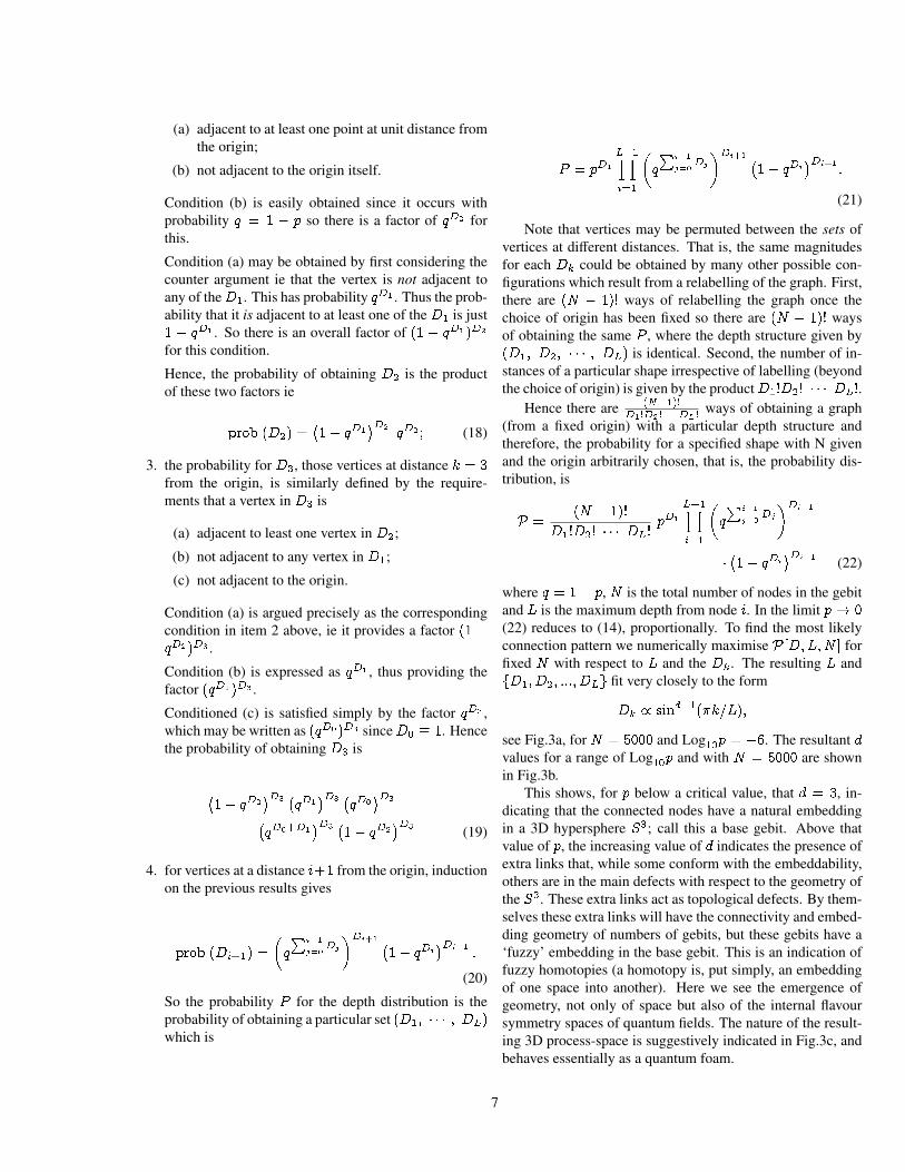
Figure 2: An N = 8 spanning tree for a random graph (not shown)with L = 3. The distance distribution Dk is indicated for node i.

disorder information system. It is important to note that Pro-cess Physics is a non-reductionist modelling of reality; the ba-sic iterator (1) is premised on the general assumption that re-ality is sufficiently complex that self-referencing occurs, andthat this has limitations. Eqn.(1) is then a minimal bootstrap-ping implementation of these notions. At higher emergentlevels this self-referencing manifests itself as interactions be-tween emergent patterns, but other novel effects may alsoarise.

To be a successful contender for the Theory of Everything(TOE) Process Physics must ultimately prove the uniquenessconjecture: that the characteristics (but not the contingent de-tails) of the pure semantic information system are unique.This would involve demonstrating both the effectiveness ofthe SOC filter and the robustness of the emergent phenomenol-ogy, and the complete agreement of the latter with observa-tion.

The stochastic neural network is modelled by the iterativeprocess

Bij ! Bij � a(B +B�1)ij +wij ; i; j = 1; 2; :::; 2N (1)

where wij = �wji are independent random variables foreach ij pair and for each iteration and chosen from someprobability distribution. Here a is a parameter the precise

2

value of which should not be critical but which influences theself-organisational process.

3 Stochastic Networks from QFTIt may be helpful to outline the thoughts that led to (1), aris-ing as it did from the quantum field theory frontier of quarkphysics. A highly effective approximation to Quantum Chro-modynamics (QCD) was developed that made extensive useof bilocal fields and the functional integral calculus (FIC), see(Cahill, 1989,1992, Cahill and Gunner 1998) for reviews ofthis Global Colour Model (GCM). In the GCM the bilocal-field correllators (giving meson and baryon correllators) aregiven by the generating functional

Z[J ] =

ZDB� exp(�S[B] +

Zd4xd4yB�(x; y)J�(x; y)):

(2)Here x; y 2 E4, namely a Euclidean-metric space-time, asthe hadronic correlators are required for vacuum-to-vacuumtransitions, and as is well known the use of the Euclideanmetric picks out the vacuum state of the quantum field theory.The physical Minkowski-metric correlators are then obtainedby analytic continuation x4 ! ix0. Eqn.(2) follows from(approximately) integrating out the gluon variables, and thenchanging variables from the quark Grassmannian functionalintegrations to bilocal-field functional integrations. Here the� index labels generators of flavour, colour and spin. Thisform is well suited to extracting hadronic phenomena as thevacuum state of QCD corresponds to a BCS-type supercon-ducting state, with the qq Cooper pairs described by thosenon-zero mean-field B

�(x; y) determined by the Euler-

Lagrange equations of the action,

�S[B]

�B�(x; y)= 0: (3)

That (3) has non-zero solutions is the constituent-quark/BCS-state effect. This is a non-linear equation for those non-zerobilocal fields about which the induced effective action forhadronic fields is to be expanded.

Rather than approximately evaluating as a functional inte-gral, as done in (Cahill, 1989,1992, Cahill and Gunner 1998),we may use the Parisi-Wu stochastic ‘quantisation’ procedure(Parisi and Wu, 1981), which involves the Langevin iterativeequation

B�(x; y)! B�(x; y)� �S[B]

�B�(x; y)+ w�(x; y); (4)

where w�(x; y) are Gaussian random variables with zeromeans. After many iterations a statistical equilibrium isachieved, and the required hadronic correllators may be ob-tained by statistical averaging: < B�(x; y)B�(u; v)::: >, but

with again analytic continuation back to Minkowski metricrequired. In particular, writing

B�(x; y) = �(x+ y

2)�(x� y; x+ y

2)

then �(x) is a meson field, while �(x;X) is the meson formfactor.

That (4) leads to quantum behaviour is a remarkable re-sult. The presence of the noise means that the full structure ofS[B] is explored during the iterations, whereas in (2) this isachieved by integration over all values of the B�(x; y) vari-ables. The correllators < B�(x; y)B�(u; v)::: > correspondto complex quantum phenomena involving bound states ofconstituent quarks embedded in a BCS superconducting state.However the Euclidean-metric E4-spacetime plays a com-pletely classical and passive background role.

Now (4) has the form of a stochastic neural network (SNN,see later), with link variablesB�(x; y), that is, with the nodesbeing continuously distributed in E4. An interesting questionarises: if we strip away the passive classical E4 backgroundand the superscript indices, so that B�(x; y) ! Bij and weretain only a simple form for S[B], then does this discretisedLangevin equation, in (1), which now even more so resem-bles a stochastic neural network, continue to display quantumbehaviour? It has been found that indeed the SNN in (1) doesexhibit quantum behaviour, by generating a quantum-foamdynamics for an emergent space, and with quantum -‘matter’being topological-defects embedded in that quantum-foam ina unification of quantum space and matter. Indeed the re-markable discovery is that (1) generates a quantum gravity.Note, however, that now the iterations in (1) correspond tophysical time, and we do not wait for equilibrium behaviour.Indeed the non-equilibrium behaviour manifests as a growinguniverse. The iterations correspond to a non-geometric mod-elling of time with an intrinsic arrow of time, as the iterationsin (1) cannot be reversed. Hence the description of this newphysics as Process Physics.

If (1) does in fact lead to a unification of gravity and quan-tum theory, then the deep question is how should we inter-pret (1)? The stochastic noise has in fact been interpreted asthe new intrinsic Self-Referential Noise when the connectionwith the work of Godel and Chaitin became apparent (Cahill,2005a). Hence beneath quantum field theory there is evi-dence of a self-referential stochastic neural network, and itsinterpretation as a semantic information system. Only by dis-carding the spacetime background of Quantum Field Theory(QFT) do we discover the necessity for space and the quan-tum.

4 Stochastic Neural NetworksWe now briefly compare the iteration system in (1) to an At-tractor Neural Network (ANN) and illustrate its basic mode

3

of operation. An ANN has link Jij 2 R and node si = �1variables (i; j = 1; 2; :::N ), with Jij = Jji and Jii = 0. Heres = +1 denotes an active node, while s = �1 denotes aninactive node. The time evolution of the nodes is given by,for example,

si(t) = sign(Xj

Jijsj(t� 1)): (5)

To imprint a pattern its si / �i values are imposed on thenodes and the Hebbian Rule is used to change the link strengths

Jij(t) = Jij(t� 1) + csi(t� 1)sj(t� 1); (6)

and for p successively stored patterns (�1; �2; :::�p) we end upwith

Jij =

pX�=1

��i �

�j ; i , j: (7)

The imprinted patterns correspond to local minima of the ‘en-ergy’ function

E[fsg] = �1

2

XJijsisj ; (8)

which has basins of attraction when the ANN is ‘exposed’ toan external input si(0). As is well known over iterations of(5) the ANN node variables converge to one of the stored pat-terns most resembling si(0). Hence the network categorisesthe external input.

The iterator (1), however, has no external inputs and itsoperation is determined by the detailed interplay between theorder/disorder terms. As well it has no node variables: whethera node i is active is determined implicitly by jBij j > b, forsome, where b is some minimum value for the link variables.Because Bij is antisymmetric and real its eigenvalues occurin pairs: ib;�ib (b real), with a complete set of orthonormaleigenvectors ��; � = �1;�2; ::;�N; (��� = ���) so that

Bjk =X

�=�1;�2;::

ib���j �

��k ; b� = �b�� 2 R; (9)

where the coefficients must occur in conjugate pairs for realBij . This corresponds to the form

B =MDM�1; D =

0BBBBBB@

0 +b1 0 0�b1 0 0 0

0 0 0 +b20 0 �b2 0

::

1CCCCCCA

(10)where M is a real orthogonal matrix. Both the b� and Mchange with each iteration.

Let us consider, in a very unrealistic situation, how pat-terns can be imprinted unchanged into the SNN. This will

only occur if we drop the B�1 term in (1). Suppose the SRNis frozen (artificially) at the same form on iteration after iter-ation. Then iterations of (1) converge to

B =1

aw =

X�

ia�1w���j �

��k ; (11)

where w� and �� are the eigensystem for w. This is analo-gous to the Hebbian rule (6), and demonstrates the imprint-ing of w, which is strong for small a. If that ‘noise’ is now‘turned-off’ then this imprinted pattern will decay, but do soslowly if a is small. Hence to maintain an unchanging im-printed pattern it needs to be continually refreshed via a fixedw. However the iterator with the B�1 term present has a sig-nificantly different and richer mode of behaviour as the sys-tem will now generate novel patterns, rather than simply im-printing whatever pattern is present in w. Indeed the systemuses special patterns (the gebits) implicit in a random w thatare used as a resource with which much more complex pat-terns are formed.

The task is to determine the nature of the self-generatedpatterns, and to extract some effective descriptive syntax forthat behaviour, remembering that the behaviour is expected tobe quantum-like.

5 Emergent Geometry in StochasticNetworks: Gebits

We start the iterations of (1) at B � 0, representing the ab-sence of information, that is, of patterns. With the noiseabsent the iterator behaves in a deterministic and reversiblemanner giving a condensate-like system with a B matrix ofthe form in (10) or (12), but with the matrixM iteration inde-pendent and determined uniquely by the start-up B, and eachb� evolves according to the iterator b� ! b� � a(b� � b�1

� ),which converges to b� = �1. The corresponding eigenvec-tors �� do not correspond to any meaningful patterns as theyare determined entirely by the random values from the start-up B � 0. However in the presence of the noise the itera-tor process is non-reversible and non-deterministic and, mostimportantly, non-trivial in its pattern generation. The itera-tor is manifestly non-geometric and non-quantum in its struc-ture, and so does not assume any of the standard features ofsyntax based non-Process Physics models. Nevertheless, aswe shall see, it generates geometric and quantum behaviour.The dominant mode is the formation of an apparently ran-domised background (in B) but, however, it also manifests aself-organising process which results in non-trivial patternswhich have the form of a growing three-dimensional frac-tal process-space displaying quantum-foam behaviour. Thesepatterns compete with this random background and representthe formation of a ‘universe’.

4

The emergence of order in this system might appear to vi-olate expectations regarding the 2nd Law of Thermodynam-ics; however because of the SRN the system behaves as anopen system and the growth of order arises from the self-referencing term, B�1 in (1), selecting certain implicit orderin the SRN. Hence the SRN acts as a source of negentropyThe term negentropy was introduced by E. Schrodinger in1944, and since then there has been ongoing discussion ofits meaning. In Process Physics it manifests as the SRN.

This growing three-dimensional fractal process-space isan example of a Prigogine far-from-equilibrium dissipativestructure driven by the SRN (Nicholis and Prigogine, 1997).From each iteration the noise term will additively introducerare large value wij . These wij , which define sets of stronglylinked nodes, will persist through more iterations than smallervalued wij and, as well, they become further linked by theiterator to form a three-dimensional process-space with em-bedded topological defects. In this way the stochastic neural-network creates stable strange attractors and as well deter-mines their interaction properties. This information is all in-ternal to the system; it is the semantic information within thenetwork.

We introduce, for convenience only, some terminology:we think of Bij as indicating the connectivity or relationalstrength between two monads i and j. The monads con-cept was introduced by Leibniz, who espoused the relationalmode of thinking in response to and in contrast with Newton’sabsolute space∗.

Bc =

0BBBBBB@

0 +1 0 0�1 0 0 00 0 0 +10 0 �1 0

::

1CCCCCCA; (12)

B =

0BBBBBBB@

g1

g2

g3c1

c2

1CCCCCCCA: (13)

The monad i has a pattern of dominant (larger valuedBij)connections Bi1; Bi2; :::, where Bij = �Bji avoids self-connection (Bii = 0), and real number valued. The self-referential noise wij = �wji are independent random vari-ables for each ij and for each iteration, and with variance �.With the noise absent the iterator converges to one of the con-densate MBcM

�1 where the matrix M depends on the ini-tial B. This behaviour is similar to the condensate of Cooper

∗However we see later that these two concepts are indeed compatible,but only by enlarging the meaning of ‘absolute space’.

pairs in QFT, but here the condensate (indicating a non-zerodominant configuration) does not have any space-like struc-ture. However in the presence of the noise, after an initialchaotic behaviour when starting the iterator from B � 0, thedominant mode is the formation of a randomised condensateC � �Bc +Bb, up to an orthogonality transformation, in-dicating Bc but with the �10s replaced by ��i’s (where the�i are small and given by a computable iteration-dependentprobability distribution M(�)) and with a noisy backgroundBb of very small Bij .

The key discovery is that there is an extremely small self-organising process buried within this condensate and whichhas the form of a three-dimensional fractal process-space,which we now explain. Consider the connectivity from thepoint of view of one monad, call it monad i. Monad i is con-nected via these large Bij to a number of other monads, andthe whole set of connected monads forms a tree-graph rela-tionship. This is because the large links are very improba-ble, and a tree-graph relationship is much more probable thana similar graph involving the same monads but with addi-tional links. The set of all large valued Bij then form tree-graphs disconnected from one-another; see Fig.2. In any onetree-graph the natural ‘distance’ measure for any two mon-ads within a graph is the smallest number of links connectingthem. Let D1; D2; :::; DL be the number of nodes of distance1; 2; ::::; L from monad i (define D0 = 1 for convenience),where L is the largest distance from i in a particular tree-graph, and let N be the total number of nodes in the tree.Then

PLk=0Dk = N ; see Fig.2 for an example.

Now consider the number N (D;N) of different randomN -node trees, with the same distance distribution fDkg, towhich i can belong. By counting the different linkage pat-terns, together with permutations of the monads we obtain

N (D;N) =(M � 1)!DD2

1 DD3

2 :::DDL

L�1

(M �N � 2)!D1!D2!:::DL!: (14)

Here DDk+1

k is the number of different possible linkage pat-terns between level k and level k + 1, and (M � 1)!=(M �N � 2)! is the number of different possible choices for themonads, with i fixed. The denominator accounts for thosepermutations which have already been accounted for by theDDk+1

k factors. We compute the most likely tree-graph struc-ture by maximising lnN (D;N) + �(

PLk=0Dk � N) where

� is a Lagrange multiplier for the constraint. Using Stirling’sapproximation for Dk! we obtain

Dk+1 = DklnDk

Dk�1� �Dk +

1

2: (15)

We may compute the most likely tree-graph structure by max-imisingN (D;N) with respect to fDkg. This equation has anapproximate analytic solution (Nagels, 1985)

Dk =2N

Lsin2(�k=L)

5

These results imply that the most likely tree-graph structureto which a monad can belong has a distance distribution fDkgwhich indicates that the tree-graph is embeddable in a 3- di-mensional hypersphere, S3.

We call these tree-graph B-sets gebits (geometrical bits).However S3 embeddability of these gebits is a weaker resultthan demonstrating the necessary emergence of S3-spaces,since extra cross-linking connections would be required forthis to produce a strong embeddability.

The monads for which the Bij are, from the SRN term,large thus form disconnected gebits, and in (13) we relabelthe monads to bring these new gebits g1; g2; g3; :: to blockdiagonal form, with the remainder indicating the small andgrowing thermalised condensate, C = c1 � c2 � c3 � ::: In(13) the gi indicate unconnected gebits, while the icon rep-resents older and connected gebits, and suggests a compact3-space. The remaining very small Bmn, not shown in (13),are background noise only.

A key dynamical feature is that most gebit matrices ghave det(g) = 0, since most tree-graph connectivity matri-ces are degenerate. For example in the tree in Fig.2 the Bmatrix has a nullspace, spanned by eigenvectors with eigen-value zero, of dimension two irrespective of the actual val-ues of the non-zero Bij ; for instance the right hand pair end-ing at the level D2 = 4 are identically connected and thiscauses two rows (and columns) to be identical up to a mul-tiplicative factor. So the degeneracy of the gebit matrix isentirely structural. For this graph there is also a second setof three monads whose connectivities are linearly dependent.These det(g) = 0 gebits form a reactive gebits subclass, i.e.in the presence of background noise (g1 � g2 � g3 � ::)�1

is well-defined and has some large elements. These reactivegebits are the building blocks of the dissipative structure. Theself-assembly process is as follows: before the formation ofthe thermalised condensate B�1 generates new connections(largeBij) almost exclusively between gebits and the remain-ing non-gebit sub-block (having det � 0 but because here allthe involved Bij � 0), resulting in the decay, without gebitinterconnection, of each gebit. However once the condensatehas formed (essentially once the system has ‘cooled’ suffi-ciently) the condensate C = c1 � c2 � c3 � ::: acts as aquasi-stable (i.e. det(C) =

Qi det(ci) , 0) sub-block of

(13) and the sub-block of gebits may be inverted separately.The gebits are then interconnected (with many gebits presentcross-links are more probable than self-links) via new linksformed by B�1, resulting in the larger structure indicated bythe in (13). Essentially, in the presence of the condensate,the gebits are sticky.

Now (14) is strictly valid in the limit of vanishingly smallprobabilities. For a more general analysis of the connectivityof such gebits assume for simplicity that the large wij arisewith fixed but very small probability p, then the emergent ge-ometry of the gebits is revealed by studying the probability

distribution for the structure of the random graph units orgebits minimal spanning trees with Dk nodes at k links fromnode i (D0 � 1), this is given more generally in the nextsection.

6 Gebit ConnectivityThe probability that a connected random graph with N ver-tices has a depth structureD0; D1; :::; DL is given in (22) andleads to the concept of emergent geometry via the gebit con-cept. Eqn.(22) was first derived by Nagels, 1985.

Consider a set of M nodes with pairwise links arising withprobability p � 1. The probability of nonlinking is thenq = 1 � p. We shall term linked nodes as being ‘adjacent’,though the use of this geometric language is to be justifiedand its limitations determined. The set M will be partitionedinto finite subsets of mutually disconnected components, eachhavingNi nodes which are at least simply connected - that is,each Ni may be described by a non-directed graph.

Consider one of these components, with N = Ni �1, and choose one vertex to be the ‘origin’. We will deter-mine the probable distribution of vertices in this componentas measured by the depth structure of a minimal spanningtree. See Fig.2 for the definition of depth structure. Let Dk

be the number of vertices at a distance k from the origin thenD0 = 1 is the origin, D1 is the number of adjacent verticesor nearest neighbours to the origin, and D2 is the number ofnext nearest neighbours and so on. Then, since N is finite,there is a maximum distance L on the graph and DL is thenumber of vertices at this maximum distance from the origin.There is then the constraint

LXk=0

Dk = N; (16)

and also 8<:

D0 = 1;Dk > 0; 0 � k � L;Dk = 0; k > L.

(17)

To calculate the probability for the distribution

fDk : 0 � k � N;

N�1Xk=0

Dk = Ng

we require:

1. the probability for the number D1 of nearest neigh-bours (i.e. those vertices at unit distance from the ori-gin) is pD1 , which may be written as (1 � q)D1 =(1� qD0

0 )D1 , since D0 = 1;

2. the probability for the next nearest neighbours, D2, isobtained by considering that any vertex at this level is

6

(a) adjacent to at least one point at unit distance fromthe origin;

(b) not adjacent to the origin itself.

Condition (b) is easily obtained since it occurs withprobability q = 1 � p so there is a factor of qD2 forthis.

Condition (a) may be obtained by first considering thecounter argument ie that the vertex is not adjacent toany of theD1. This has probability qD1 . Thus the prob-ability that it is adjacent to at least one of the D1 is just1 � qD1 . So there is an overall factor of (1 � qD1)D2

for this condition.

Hence, the probability of obtaining D2 is the productof these two factors ie

prob (D2) =�1� qD1

�D2

qD2 ; (18)

3. the probability for D3, those vertices at distance k = 3from the origin, is similarly defined by the require-ments that a vertex in D3 is

(a) adjacent to least one vertex in D2;

(b) not adjacent to any vertex in D1;

(c) not adjacent to the origin.

Condition (a) is argued precisely as the correspondingcondition in item 2 above, ie it provides a factor (1 �qD2)D3 .

Condition (b) is expressed as qD1 , thus providing thefactor (qD1)D3 .

Conditioned (c) is satisfied simply by the factor qD3 ,which may be written as (qD0)D3 sinceD0 � 1. Hencethe probability of obtaining D3 is

�1� qD2

�D3�qD1�D3

�qD0�D3

=�qD0+D1

�D3�1� qD2

�D3 (19)

4. for vertices at a distance i+1 from the origin, inductionon the previous results gives

prob (Di+1) =

�q

Pi�1

j=0Dj

�Di+1 �1� qDi

�Di+1:

(20)

So the probability P for the depth distribution is theprobability of obtaining a particular set (D1; � � � ; DL)which is

P = pD1

L�1Yi=1

�q

Pi�1

j=0Dj

�Di+1 �1� qDi

�Di+1:

(21)

Note that vertices may be permuted between the sets ofvertices at different distances. That is, the same magnitudesfor each Dk could be obtained by many other possible con-figurations which result from a relabelling of the graph. First,there are (N � 1)! ways of relabelling the graph once thechoice of origin has been fixed so there are (N � 1)! waysof obtaining the same P , where the depth structure given by(D1; D2; � � � ; DL) is identical. Second, the number of in-stances of a particular shape irrespective of labelling (beyondthe choice of origin) is given by the productD1!D2! � � � DL!.

Hence there are (N�1)!D1!D2! ��� DL!

ways of obtaining a graph(from a fixed origin) with a particular depth structure andtherefore, the probability for a specified shape with N givenand the origin arbitrarily chosen, that is, the probability dis-tribution, is

P =(N � 1)!

D1!D2! � � � DL!pD1

L�1Yi=1

�q

Pi�1

j=0Dj

�Di+1

� �1� qDi�Di+1 (22)

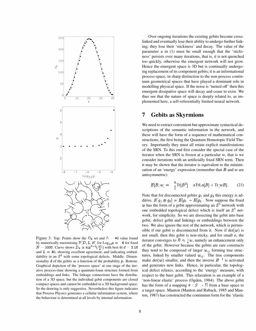
where q = 1� p, N is the total number of nodes in the gebitand L is the maximum depth from node i. In the limit p! 0(22) reduces to (14), proportionally. To find the most likelyconnection pattern we numerically maximise P[D;L;N ] forfixed N with respect to L and the Dk. The resulting L andfD1; D2; :::; DLg fit very closely to the form

Dk / sind�1(�k=L);

see Fig.3a, for N = 5000 and Log10p = �6. The resultant dvalues for a range of Log10p and with N = 5000 are shownin Fig.3b.

This shows, for p below a critical value, that d = 3, in-dicating that the connected nodes have a natural embeddingin a 3D hypersphere S3; call this a base gebit. Above thatvalue of p, the increasing value of d indicates the presence ofextra links that, while some conform with the embeddability,others are in the main defects with respect to the geometry ofthe S3. These extra links act as topological defects. By them-selves these extra links will have the connectivity and embed-ding geometry of numbers of gebits, but these gebits have a‘fuzzy’ embedding in the base gebit. This is an indication offuzzy homotopies (a homotopy is, put simply, an embeddingof one space into another). Here we see the emergence ofgeometry, not only of space but also of the internal flavoursymmetry spaces of quantum fields. The nature of the result-ing 3D process-space is suggestively indicated in Fig.3c, andbehaves essentially as a quantum foam.

7

0 10 20 30 40

k

0

50

100

150

200

250

Dk

-8 -7 -6 -5 -4

Log10p

2

3

4

5

6

d

Figure 3: Top: Points show the Dk set and L = 40 value foundby numerically maximising P[D;L;N ] for Log

10p = �6 for fixed

N = 5000. Curve shows Dk / sind�1(�kL) with best fit d = 3:16

and L = 40, showing excellent agreement, and indicating embed-dability in an S3 with some topological defects. Middle: Dimen-sionality d of the gebits as a function of the probability p. Bottom:Graphical depiction of the ‘process space’ at one stage of the iter-ative process-time showing a quantum-foam structure formed fromembeddings and links. The linkage connections have the distribu-tion of a 3D space, but the individual gebit components are closedcompact spaces and cannot be embedded in a 3D background space.So the drawing is only suggestive. Nevertheless this figure indicatesthat Process Physics generates a cellular information system, wherethe behaviour is determined at all levels by internal information.

Over ongoing iterations the existing gebits become cross-linked and eventually lose their ability to undergo further link-ing; they lose their ‘stickiness’ and decay. The value of theparameter a in (1) must be small enough that the ‘sticki-ness’ persists over many iterations, that is, it is not quenchedtoo quickly, otherwise the emergent network will not grow.Hence the emergent space is 3D but is continually undergo-ing replacement of its component gebits; it is an informationalprocess-space, in sharp distinction to the non-process contin-uum geometrical spaces that have played a dominant role inmodelling physical space. If the noise is ‘turned off’ then thisemergent dissipative space will decay and cease to exist. Wethus see that the nature of space is deeply related to, as im-plemented here, a self-referentially limited neural network.

7 Gebits as SkyrmionsWe need to extract convenient but approximate syntactical de-scriptions of the semantic information in the network, andthese will have the form of a sequence of mathematical con-structions, the first being the Quantum Homotopic Field The-ory. Importantly they must all retain explicit manifestationsof the SRN. To this end first consider the special case of theiterator when the SRN is frozen at a particular w, that is weconsider iterations with an artificially fixed SRN term. Thenit may be shown that the iterator is equivalent to the minimi-sation of an ‘energy’ expression (remember that B and w areantisymmetric)

E[B;w] = �a2

Tr[B2]� aTrLn[B] + Tr[wB]: (23)

Note that for disconnected gebits g1 and g2 this energy is ad-ditive, E[g1 � g2] = E[g1] + E[g2]. Now suppose the fixedw has the form of a gebit approximating an S3 network withone embedded topological defect which is itself an S3 net-work, for simplicity. So we are dissecting the gebit into basegebit, defect gebit and linkings or embeddings between thetwo. We also ignore the rest of the network, which is permis-sible if our gebit is disconnected from it. Now if det(w) isnot small, then this gebit is non-sticky, and for small a, theiterator converges to B � 1

aw, namely an enhancement only

of the gebit. However because the gebits are rare constructsthey tend to be composed of larger wij forming tree struc-tures, linked by smaller valued wij . The tree componentsmake det(w) smaller, and then the inverse B�1 is activatedand generates new links. Hence, in particular, the topolog-ical defect relaxes, according to the ‘energy’ measure, withrespect to the base gebit. This relaxation is an example of a‘non-linear elastic’ process (Ogden, 1984). The above gebithas the form of a mapping � : S ! � from a base space toa target space. Manton (Manton and Ruback, 1985 and Man-ton, 1987) has constructed the continuum form for the ‘elastic

8

energy’ of such an embedding and for � : S3 ! S3 it is theSkyrme energy

E[U ] =

Z ��1

2Tr(@iUU�1@iUU

�1)�1

16Tr[@iUU�1; @iUU

�1]2�; (24)

where U(x) is an element of SU(2). Via the parametrisationU(x) = �(x) + i~�(x):~� , where the �i are Pauli matrices,we have �(x)2 + ~�(x)2=1, which parametrises an S3 as aunit hypersphere embedded in E4 (which has no ontologi-cal significance, of course). Non-trivial minima of E[U ] areknown as Skyrmions (a form of topological soliton), and haveZ = �1;�2; :::, where Z is the winding number of the map,

Z =1

24�2

Z X�ijkTr(@iUU�1@jUU

�1@kUU�1): (25)

The first key to extracting emergent phenomena from thestochastic neural network is the validity of this continuumanalogue, namely that E[B;w] and E[U ] are describing es-sentially the same ‘energy’ reduction process. This requiresdetailed analysis.

8 Absence of a Cosmic CodeThis ‘frozen’ SRN analysis of course does not match the time-evolution of the full iterator (1), for this displays a muchricher collection of processes. With ongoing new noise ineach iteration and the saturation of the linkage possibilities ofthe gebits emerging from this noise, there arises a process ofongoing birth, linking and then decay of most patterns. Thetask is then to identify those particular patterns that survivethis flux, even though all components of these patterns even-tually disappear, and to attempt a description of their modesof behaviour. This brings out the very biological nature of theinformation processing in the SNN, and which appears to becharacteristic of a ‘pure’ semantic information system. Kitto2002 has further investigated the analogies between ProcessPhysics and living systems. The emergent ‘laws of physics’are the habitual habits of this system, and it appears that theymay be identified. However there is no encoding mechanismfor these ‘laws’, they are continually manifested; there is nocosmic code. In contrast living or biological systems could bedefined as those emergent patterns which discovered how toencode their ‘laws’ in a syntactical genetic code. Neverthe-less such biological systems make extensive use of semanticinformation at all levels as their genetic code is expressed inthe phenotype.

9 Entrapped Topological DefectsIn general each gebit, as it emerges from the SRN, has activenodes and embedded topological defects, again with activenodes. Further there will be defects embedded in the defectsand so on, and so gebits begin to have the appearance of afractal defect structure, and with all the defects having variousclassifications and associated winding numbers. The energyanalogy above suggests that defects with opposite windingnumbers at the same fractal depth may annihilate by drift-ing together and merging. Furthermore the embedding of thedefects is unlikely to be ‘classical’, in the sense of being de-scribed by a mapping �(x), but rather would be fuzzy, i.edescribed by some functional, F [�], which would correspondto a classical embedding only if F has a very sharp supremumat one particular � = �cl. As well these gebits are undergo-ing linking because their active nodes (see Cahill and Klinger2000 for more discussion) activate theB�1 new-links processbetween them, and so by analogy the gebits themselves formlarger structures with embedded fuzzy topological defects.This emergent behaviour is suggestive of a quantum spacefoam, but one containing topological defects which will bepreserved by the system, unless annihilation events occur. Ifthese topological defects are sufficiently rich in fractal struc-ture so as to be preserved, then their initial formation wouldhave occurred as the process-space relaxed out of its initialessentially random form. This phase would correspond to theearly stages of the Big-Bang. Once the topological defectsare trapped in the process-space they are doomed to meanderthrough that space by essentially self-replicating, i.e. contin-ually having their components die away and be replaced bysimilar components. These residual topological defects arewhat we call matter. The behaviour of both the process-spaceand its defects is clearly determined by the same network pro-cesses; we have an essential unification of space and mat-ter phenomena. This emergent quantum foam-like behavioursuggests that the full generic description of the network be-haviour is via the Quantum Homotopic Field Theory (QHFT).We also see that cellular structures are a general feature of se-mantic information systems, with the information necessarilydistributed.

10 Functional Schrodinger EquationBecause of the iterator the resource is the large valued Bij

from the SRN because they form the ‘sticky’ gebits which areself-assembled into the non-flat compact 3D process-space.The accompanying topological defects within these gebits andalso the topological defects within the process space require amore subtle description. The key behavioural mode for thosedefects which are sufficiently large (with respect to the num-ber of component gebits) is that their existence, as identifiedby their topological properties, will survive the ongoing pro-

9

cess of mutation, decay and regeneration; they are topologi-cally self-replicating. Consider the analogy of a closed loopof string containing a knot - if, as the string ages, we replacesmall sections of the string by new pieces then eventually allof the string will be replaced, however the relational informa-tion represented by the knot will remain unaffected as onlythe topology of the knot is preserved. In the process-spacethere will be gebits embedded in gebits, and so forth, in topo-logically non-trivial ways; the topology of these embeddingsis all that will be self-replicated in the processing of the dis-sipative structure.

To analyse and model the ‘life’ of these topological de-fects we need to characterise their general behaviour: if suf-ficiently large (i) they will self-replicate if topological non-trivial, (ii) we may apply continuum homotopy theory to tellsus which embeddings are topologically non-trivial, (iii) de-fects will only dissipate if embeddings of ‘opposite windingnumber’ (these classify the topology of the embedding) en-gage one another, (iv) the embeddings will be in general frac-tal, and (iv) the embeddings need not be ‘classical’, ie theembeddings will be fuzzy. To track the coarse-grained be-haviour of such a system led to the development of a newform of quantum field theory: Quantum Homotopic FieldTheory (QHFT). This models both the process-space and thetopological defects.

Figure 4: An representation of the functional [f�g; t] showingdominant homotopies. The ‘magnifying glass’ indicates that thesemappings can be nested. Graphic by C. Klinger.

To construct this QHFT we introduce an appropriate con-figuration space, namely all the possible homotopic mappings��� : S� ! S�, where the S1; S2; ::, describing ‘clean’or topological-defect free gebits, are compact spaces of var-ious types. Then QHFT has the form of an iterative func-tional Schrodinger equation for the discrete time-evolution ofa wave-functional [::::; ��� ; ::::; t]

[::::; ��� ; ::::; t+�t] = [::::; ��� ; ::::; t]�iH[::::; ��� ; ::::; t]�t+ QSD terms: (26)

This form arises as it is models the preservation of seman-tic information, by means of a unitary time evolution; even

in the presence of the noise in the Quantum State Diffusion(QSD, Percival, 1998) terms. Because of the QSD noise (26)is an irreversible quantum system. The time step �t in (26)is relative to the scale of the fractal processes being explicitlydescribed, as we are using a configuration space of mappingsbetween prescribed gebits. At smaller scales we would need asmaller value for �t. Clearly this invokes a (finite) renormal-isation scheme. We now discuss the form of the hamiltonianand the QSD terms.

First (26), without the QSD term, has a form analogousto a ‘third quantised’ system, in conventional terminology(Coleman et al. 2000). These systems were considered asperhaps capable of generating a quantum theory of gravity.The argument here is that this is the emergent behaviour ofthe SNN, and it does indeed lead to quantum gravity, but withquantum matter as well. More importantly we understand theorigin of (26), and it will lead to quantum and then classicalgravity, rather than arise from classical gravity via some adhoc or heuristic quantisation procedure.

Depending on the ‘peaks’ of and the connectivity of theresultant dominant mappings such mappings are to be inter-preted as either embeddings or links; Fig.4 then suggests thedominant process-space form within showing both linksand embeddings. The emergent process-space then has thecharacteristics of a quantum foam. Note that, as indicated inFig.4, the original start-up links and nodes are now absent.Contrary to the suggestion in Fig.4, this process space cannotbe embedded in a finite dimensional geometric space with theemergent metric preserved, as it is composed of nested finite-dimensional closed spaces.

11 Homotopy HamiltonianWe now consider the form of the hamiltonian H. In the previ-ous sections it was suggested that Manton’s non-linear elas-ticity interpretation of the Skyrme energy is appropriate to theSNN. This then suggests that H is the functional operator

H =X�,�

h[�

����; ��� ]; (27)

where h[ ���; �] is the (quantum) Skyrme Hamiltonian func-

tional operator for the system based on making fuzzy themappings � : S ! �, by having h act on wave-functionalsof the form [�(x); t]. Then H is the sum of pairwise em-bedding or homotopy hamiltonians. The corresponding func-tional Schrodinger equation would simply describe the timeevolution of quantised Skyrmions with the base space fixed,and � 2 SU(2). There have been very few analyses of thisclass of problem, and then the base space is usually taken tobe E3. We shall not give the explicit form of h as it is com-plicated, but wait to present the associated action.

10

In the absence of the QSD terms the time evolution in (26)can be formally written as a functional integral

[f�g; t0] =Z Y

�,�

D~���eiS[f~�g][f�g; t]; (28)

where, using the continuum t limit notation, the action is asum of pairwise actions,

S[f~�g] =X�,�

S�� [~��� ]; (29)

S�� [~�] =

Z t0

t

dt00Zdnx

p�g�1

2Tr(@� ~U ~U�1@� ~U ~U�1)+

1

16Tr[@� ~U ~U�1; @� ~U ~U�1]2

�

and the now time-dependent (indicated by the tilde symbol)mappings ~� are parametrised by ~U(x; t), ~U 2 S�. The met-ric g�� is that of the n-dimensional base space, S� , in ��;� :S� ! S�. As usual in the functional integral formalism thefunctional derivatives in the quantum hamiltonian, in (27),now manifest as the time components @0 in the above equa-tion, so now this has the form of a ‘classical’ action, and wesee the emergence of ‘classical’ fields, though the emergenceof ‘classical’ behaviour is a more complex process. Eqns.(26)or (28) describe an infinite set of quantum skyrme systems,coupled in a pairwise manner. Note that each homotopic map-ping appears in both orders; namely ��� and ���.

12 Quantum State DiffusionThe Quantum State Diffusion (QSD) (Percival, 1998) termsare non-linear and stochastic,

QSD =Xj

�<L

yj> Lj � 1

2LyjLj� <L

yj><Lj>

��t+

Xj

(Lj� <Lj>)��j ; (30)

which involves summation over the class of Linblad func-tional operators Lj . The QSD terms are up to 5th order in, as in general

<A>t�Z Y

�,�

D���[f�g; t]�A[f�g; t] (31)

and where ��j are complex statistical variables with meansM(��j) = 0, M(��j��j0) = 0 and M(���j��j0) = �(j �j0)�t. The remarkable property of this QSD term is that theunitarity of the time evolution in (26) is maintained in themean.

13 Emergent ClassicalityThese QSD terms are ultimately responsible for the emer-gence of classicality via an objectification (Percival 1998),but in particular they produce wave-function(al) collapses dur-ing quantum measurements, as the QSD terms tend to ‘sharpen’the fuzzy homotopies towards classical or sharp homotopies.So the QSD terms, as residual SRN effects, lead to the Bornquantum measurement random behaviour, but here arisingfrom the Process Physics, and not being invoked as a metarule.Keeping the QSD terms leads to a functional integral repre-sentation for a density matrix formalism in place of (28), andthis amounts to a derivation of the decoherence formalismwhich is usually arrived at by invoking the Born measure-ment metarule. Here we see that decoherence arises from thelimitations on self-referencing.

In the above we have a deterministic and unitary evo-lution, tracking and preserving topologically encoded infor-mation, together with the stochastic QSD terms, whose formprotects that information during localisation events, and whichalso ensures the full matching in QHFT of process-time toreal time: an ordering of events, an intrinsic direction or ‘ar-row’ of time and a modelling of the contingent present mo-ment effect. So we see that Process Physics generates a com-plete theory of quantum measurements involving the non-local, non-linear and stochastic QSD terms. It does this be-cause it generates both the ‘objectification’ process associ-ated with the classical apparatus and the actual process of(partial) wavefunctional collapse as the quantum modes in-teract with the measuring apparatus. Indeed many of themysteries of quantum measurement are resolved when it isrealised that it is the measuring apparatus itself that activelyprovokes the collapse, and it does so because the QSD pro-cess is most active when the system deviates strongly fromits dominant mode, namely the ongoing relaxation of the sys-tem to a 3D process-space, and matter survives only becauseof its topological form. This collapse amounts to an ongo-ing sharpening of the homotopic mappings towards a ‘clas-sical’ 3D configuration - resulting in essentially the processwe have long recognised as ‘space’. Being non-local the col-lapse process does not involve any propagation effects, that isthe collapse does not require any effect to propagate throughthe space. For that reason the self-generation of space is insome sense action-at-a-distance, and the emergence of sucha quantum process underlying reality is, of course, contraryto the long-held belief by physicists that such action is unac-ceptable, though that belief arose before the quantum collapsewas experimentally shown to display action at a distance inthe Aspect experiment. Hence we begin to appreciate why thenew theory of gravity does not involve the maximum speed cof propagation through space. and why it does not predict theGR gravitational waves travelling at speed c, of the kind longsearched for but not detected.

11

The mappings ��� are related to group manifold param-eter spaces with the group determined by the dynamical sta-bility of the mappings. This symmetry leads to the flavoursymmetry of the standard model of ‘particle’ physics. Quan-tum homotopic mappings or skyrmions behave as fermionicor bosonic modes for appropriate winding numbers; so Pro-cess Physics predicts both fermionic and bosonic quantummodes, but with these associated with topologically encodedinformation and not with objects or ‘particles’.

14 Emergent Quantum Field TheoryThe QHFT is a very complex ‘book-keeping’ system for theemergent properties of the neural network, and we now sketchhow we may extract a more familiar Quantum Field Theory(QFT) that relates to the standard model of ‘particle’ physics.An effective QFT should reproduce the emergence of theprocess-space part of the quantum foam, particularly its 3Daspects. The QSD processes play a key role in this as theytend to enhance classicality. Hence at an appropriate scaleQHFT should approximate to a more conventional QFT, namelythe emergence of a wave-functional system [U(x); t] wherethe configuration space is that of homotopies from a 3-spaceto U(x) 2 G, where G is some group manifold space. ThisG describes ‘flavour’ degrees of freedom. So we are coarse-graining out the gebit structure of the quantum-foam. Hencethe Schrodinger wavefunctional equation for this QFT willhave the form

[U ; t+�t] = [U ; t]� iH[U ; t]�t+QSD terms; (32)

where the general form of H is known, and where a newresidual manifestation of the SRN appears as the new QSDterms. This system describes skyrmions embedded in a con-tinuum space. It is significant that such Skyrmions are onlystable, at least in flat space and for static skyrmions, if thatspace is 3D. This tends to confirm the observation that 3Dspace is special for the neural network process system.

15 Emergent Flavour and ColourAgain, in the absence of the QSD terms, we may express (32)in terms of the functional integral

[U ; t0] =

ZD ~UeiS[

~U ][U ; t]: (33)

To gain some insight into the phenomena present in (32) or(33), it is convenient to use the fact that functional integrals ofthis Skyrmionic form my be written in terms of Grassmann-variable functional integrals, but only by introducing a ficti-tious ‘metacolour’ degree of freedom and associated colouredfictitious vector bosons. This is essentially the reverse of the

xx~~

hhhhhhhhhhhhhhhhjjjj

Figure 5: The is a representation of the origin of quantum non-locality. An entity is attached at two disjoint regions of the [3]-space,with the gebit structure of that space not shown.

Functional Integral Calculus (FIC) hadronisation technique inthe Global Colour Model (GCM) of QCD. The action for theGrassmann and vector boson part of the system is of the form(written for flat space)

S[p; p; Aa�] =

Zd4x

�p �(i@� + g

�a

2Aa�)p�

1

4F a��(A)F

a��(A)

�; (34)

where the Grassmann variables pfc(x) and pfc(x) have flavourand metacolour labels. The Skyrmions are then re-constructed,in this system, as topological solitons. These coloured andflavoured but fictitious fermionic fields p and p correspondto a preon system. As they are purely fictitious, in the sensethat there are no excitations in the system corresponding tothem, the metacolour degree of freedom must be hidden orconfined. We thus arrive at the general feature of the standardmodel of particles with flavour and confined colour degreesof freedom. Then while the QHFT and the QFT representan induced syntax for the semantic information, the preonsmay be considered as an induced ‘alphabet’ for that syntax.The advantage of introducing this preon alphabet is that wecan more easily determine the states of the system by usingthe more familiar language of fermions and bosons, ratherthan working with the skyrmionic system, so long as onlycolour singlet states are finally permitted. In order to estab-lish fermionic behaviour a Wess-Zumino (WZ) process mustbe extracted from the iterator behaviour or the QHFT. Such aWZ process is time-dependent, and so cannot arise from thefrozen SRN. It is important to note that (34) and the action in(33) are certainly not the final forms. Further analysis will berequired to fully extract the induced actions for the emergentQFT.

16 Hilbert SpacesProcess Physics has suggested the origin of quantum phe-nomena and of its Hilbert-space formalism. This phenomenais associated with the time evolution of the conserved topo-logical defects embedded in the process space. However that

12

embedding need not be local, as illustrated in Fig.5. This par-ticular situation corresponds to the Hilbert space ‘sum’

(x) = 1(x) + 2(x); (35)

where 1(x) and 2(x) are non-zero only in the respectiveembedding regions. This is how quantum non-locality man-ifests in conventional quantum theory. So the Hilbert space‘sum’ is the representation of the connectivity shown in Fig.5.Such a non-local embedding is also responsible for the phe-nomenon of quantum entanglement.

17 Quantum Matter and DynamicalSpace

The dynamics and detection of space is a phenomenon thatphysics missed from its beginning, with space modelled as ageometric entity without structure or time dependence. Thathas changed recently with the determination of the speed anddirection of the solar system through the dynamical space,and the characterisation of the flow turbulence: gravitationalwaves. Detections used various techniques and have all pro-duced the same speed and direction (Cahill 2005b - 2014b) .The detected dynamical space was missing from all conven-tional theories in physics: Gravity, Electromagnetism, Atomic,Nuclear, Climate,... The detection of the dynamical space hasled to a major new and extensively tested theory of reality.

Above we presented a “bottom up” theory. Here we presenta “top down” theory that follows from a minimal extension ofthe quantum theory and the gravity theory by introducing thedetected dynamical space.

The Schrodingier equation extension to include the dy-namical space is, Cahill 2006c,

i~@ (r; t)

@t= � ~

2

2mr2 (r; t) + V (r; t) (r; t) +

�i~�v(r; t)�r+

1

2r�v(r; t)

� (r; t) (36)

Here v(r; t) is the velocity field describing the dynamicalspace at a classical field level, and the coordinates r givethe relative location of (r; t) and v(r; t), relative to a Eu-clidean embedding space, and also used by an observer tolocate structures. At sufficiently small distance scales thatembedding and the velocity description is conjectured to benot possible, as then the dynamical space requires an indeter-minate dimension embedding space, being possibly a quan-tum foam, as noted above. This minimal generalisation ofthe original Schrodingier equation arises from the replace-ment @=@t ! @=@t + v:r, which ensures that the quantumsystem properties are determined by the dynamical space,and not by the embedding coordinate system. The same re-placement is also to be implemented in the original Maxwell

equations, yielding that the speed of light is constant onlywrt the local dynamical space, as observed, and which re-sults in lensing from stars and black holes. The extra r�v term in (36) is required to make the hamiltonian in (36)hermitian. Essentially the existence of the dynamical spacein all theories has been missing. The dynamical theory ofspace itself is briefly reviewed below. The dynamical spacevelocity has been detected with numerous techniques, dat-ing back to the 1st detection, the Michelson-Morley experi-ment of 1887, which was misunderstood, and which lead tophysics developing flawed theories of the various phenomenanoted above. A particularly good technique used the NASADoppler shifts from spacecraft Earth-flybys, Cahill 2009b, todetermine the anisotropy of the speed of EM waves. All suc-cessful detection techniques have observed significant fluctu-ations in speed and direction: these are the actually “gravita-tional waves”, because they are associated with gravitationaland other effects. In particular we report here the role ofthese waves in solar flare excitations and Earth climate sci-ence (Cahill, 2014b).

A significant effect follows from (36), namely the emer-gence of gravity as a quantum effect: a wave packet analysisshows that the acceleration of a wave packet, due to the spaceterms alone (when V (r; t) = 0), given by g = d2<r>=dt2,(Cahill, 2006c), gives

g(r; t) =@v

@t+ (v� r)v (37)

That derivation showed that the acceleration is independentof the mass m: whence we have the 1st derivation of theWeak Equivalence Principle, discovered experimentally byGalileo. As noted below the dynamical theory for v(r; t) hasexplained numerous gravitational phenomena.

The experimental data reveals the existence of a dynam-ical space. It is a simple matter to arrive at the dynamicaltheory of space, and the emergence of gravity as a quantummatter effect, as noted above. The key insight is to note thatthe emergent quantum-theoretic matter acceleration in (37),@v=@t+ (v� r)v, is also, and independently, the constituentEuler acceleration a(r; t) of the space flow velocity field,

a(r; t) = lim�t!0

v(r+ v(r; t)�t; t+�t)� v(r; t)

�t

=@v

@t+ (v�r)v (38)

which describes the acceleration of a constituent element ofspace by tracking its change in velocity. This means thatspace has a structure that permits its velocity to be defined anddetected, which experimentally has been done. This then sug-gests, from (37) and (38), that the simplest dynamical equa-tion for v(r; t) is

r��@v

@t+ (v�r)v

�= �4�G�(r; t); r� v = 0 (39)

13

because it then givesr:g = �4�G�(r; t); r�g = 0, whichis Newton’s inverse square law of gravity in differential form.Hence the fundamental insight is that Newton’s gravitationalacceleration field g(r; t) for matter is really the accelerationfield a(r; t) of the structured dynamical space, and that quan-tum matter acquires that acceleration because it is fundamen-tally a wave effect, and the wave is refracted by the accelera-tions of space.

While the above leads to the simplest 3-space dynamicalequation this derivation is not complete yet. One can add ad-ditional terms with the same order in speed spatial derivatives,and which cannot be a priori neglected. There are two suchterms, as in

r��@v

@t+ (v�r)v

�+5�

4

�(trD)2 � tr(D2)

�+::: = �4�G�

where Dij = @vi=@xj . However to preserve the inversesquare law external to a sphere of matter the two terms musthave coefficients � and ��, as shown. Here � is a dimen-sionless space self-interaction coupling constant, which ex-perimental data reveals to be, approximately, the fine struc-ture constant, � = e2=~c. The ellipsis denotes higher orderderivative terms with dimensioned coupling constants, whichcome into play when the flow speed changes rapidly wrt dis-tance. The observed dynamics of stars and gas clouds nearthe centre of the Milky Way galaxy has revealed the need forsuch a term (Cahill and Kerrigan, 2011), and we find that thespace dynamics then requires an extra term:

r��@v

@t+ (v�r)v

�+

5�

4

�(trD)2 � tr(D2)

�+

+�2r2�(trD)2 � tr(D2)

�+ ::: = �4�G� (40)

where � has the dimension of length, and appears to be a verysmall Planck-like length. This then gives us the dynamicaltheory of 3-space. It can be thought of as arising via a deriva-tive expansion from a deeper theory, such as a quantum foamtheory, above. Note that the equation does not involve c, isnon-linear and time-dependent, and involves non-local directinteractions. Its success implies that the universe is more con-nected than previously thought. Even in the absence of matterthere can be time-dependent flows of space.

Note that the dynamical space equation, apart from theshort distance effect - the � term, there is no scale factor, andhence a scale free structure to space is to be expected, namelya fractal space. That dynamical equation has back hole andcosmic filament solutions (Cahill and Kerrigan, 2011, Rothalland Cahill, 2013), which are non-singular because of the ef-fect of the � term. At large distance scales it appears that ahomogeneous space is dynamically unstable and undergoesdynamical breakdown of symmetry to form a spatial networkof black holes and filaments, (Rothall and Cahill, 2013), towhich matter is attracted and coalesces into gas clouds, starsand galaxies.

Figure 6: Representation of the fractal wave data revealing thefractal textured structure of the 3-space, with cells of space havingslightly different velocities and continually changing, and movingwrt the Earth with a speed of �500 km/s, and from a southerly di-rection, namely almost perpendicular to the plane of the ecliptic.This “pink space” is suggestive of the 1/f spectrum of the detectedfluctuations.

The dynamical space equation (40) explains phenomenasuch as Earth bore-hole gravity anomalies, from which thevalue of � was extracted, flat rotation curves for spiral galax-ies, galactic black holes and cosmic filaments, the universegrowing/expanding at almost a constant rate, weak and stronggravitational lensing of light,.... A significant aspect of thespace dynamics is that space is not conserved: it is continu-ally growing, giving the observed universe expansion, and isdissipated by matter. As well it has no energy density mea-sure. Nevertheless it can generate energy into matter.

18 Detecting Dynamical Space Speedand Turbulence with Diodes

The Zener diode in reverse bias mode can easily and reliablymeasure the space speed fluctuations, Fig.7, and two such de-tectors can measure the speed and direction of the space flowand waves, (Cahill, 2013c - 2014b). Consider plane waveswith energy E = ~!. Then (36) with v = 0 and V = 0gives = e�!t+ik�r. When v , 0, but locally uniform wrtto the diode, the energy becomes E ! E + ~k � v. Thisenergy shift can be easily detected by the diode as the elec-tron transmission current increases with increased energy. Byusing spatially separated diodes the speed and direction hasbeen measured, and agrees with other detection techniques.

Although this Zener diode effect was only discovered in2013, (Cahill, 2013c), Zener diode detectors have been avail-able commercially for much longer, and are known as Ran-dom Event Generators, (REG). That terminology was basedon the flawed assumption that the quantum tunnelling fluctua-tions were random wrt an average. However the data (Cahill,

14

Figure 7: Circuit of Zener Diode Gravitational Wave Detector,showing 1.5V AA battery, one 1N4728A Zener diodes operating inreverse bias mode, and having a Zener voltage of 3.3V, and resistorR= 10K. Voltage V across resistor is measured and used to de-termine the space driven fluctuating tunnelling current through theZener diodes. Current fluctuations from two collocated detectors areshown to be the same, but when spatially separated there is a timedelay effect, so the current fluctuations are caused by space speedfluctuations. Using diodes in parallel increases S/N.

2013c) showed that this is not the case. That experimental re-sult contradicts the standard interpretation of “randomness”in quantum processes, which dates back to the Born interpre-tation in 1926. To the contrary the recent experiments showthat the fluctuations are not random, but are directly deter-mined by the fluctuations in the passing dynamical space.

The various detections of the dynamical space alwaysshowed turbulence/wave effects, and we can represent thefractal structure of this space in Fig.6.

19 Neo-Lorentz RelativityThe major extant relativity theories - Galileo’s Relativity(GaR), Lorentz’s Relativity (LR) and Einstein’s Special Rel-ativity (SR), with the latter much celebrated, while the LR isessentially ignored. Indeed it is often incorrectly claimed thatSR and LR are experimentally indistinguishable. It has beenshown that (i) SR and LR are experimentally distinguishable,(ii) that comparison of gas-mode Michelson interferometerexperiments with spacecraft earth-flyby Doppler shift datademonstrate that it is LR that is consistent with the data, whileSR is in conflict with the data, (iii) SR is exactly derivablefrom GaR by means of a mere linear change of space andtime coordinates that mixes the Galilean space and time coor-dinates (Cahill, 2013a). So it is GaR and SR that are equiva-lent. Hence the well-known SR relativistic effects are purelycoordinate effects, and cannot correspond to the observed rel-ativistic effects. The connections between these three rela-tivity theories has become apparent following the discoverythat space is an observable dynamical textured system, andthat space and time are distinct phenomena, leading to a neo-Lorentz Relativity (nLR). The observed relativistic effects are

dynamical consequences of nLR and 3-space. In particular inSR length contraction of rods and time dilation of clocks aresupposedly caused only by motion wrt the observer, whereasin nLR these effects are caused by motion wrt the space lo-cal to the rods and clocks, and apply only to actual rods andclocks. In the case of Maxwell’s EM theory the dynamicalspace is incorporated into the vacuum field equation by mak-ing the change @=@t! @=@t+ v � r (Cahill 2009a).

20 ConclusionsThe discovery that a dynamical space exists by Cahill andKitto 2003 represented a dramatic turning point in our under-standing of reality, since until then physicists had assumedthat space and time, or even spacetime, were successful purelygeometrical modellings of the phenomena of space and time,and denied any notion that a dynamical 3-space exists whichdisplays a flow velocity wrt an observer, and which displaysturbulence/gravitational wave effects. These are now easy tomeasure and characterise, exhibiting a fractal time dependentstructure. This space is fundamental to all phenomena, andwe are now entering a new epoch in physics in which therole of space in all phenomena is now emerging, see for ex-ample the recent discoveries re solar flares and earth climate,(Cahill 2014b). Here we have reviewed two related aspectsof this new physics: first we considered reality to be a self-referencing stochastic network, and showed that there is evi-dence that a dynamical fractal space arises and with quantummatter also arising as topological defects in the space. As wellwe have briefly discussed the consequences of modifying the-ories of the quantum, EM radiation and gravity by includinga dynamical space modelled at the classical level by a veloc-ity field. Of key significance is that in recent years a vari-ety of new 3-space detection technologies have been devised,with the latest being the nanotechnology pn diode detectiondevice, which is incredibly simple, cheap and robust. Thesuccess of that device demonstrated the the standard interpre-tation of “quantum randomness” was incorrect, namely thatthe observed fluctuations were caused by the space passingthrough the diode.

21 References

Cahill, R.T., 1989. Hadronisation of QCD, Aust. J. Phys. 42,171.

Cahill R.T., 1992. Hadronic Laws from QCD, Nucl. Phys. A,543, 63.

Cahill R.T. and Gunner S.M., 1998. The Global Colour Modelof QCD for Hadronic Processes: A Review, Fizika B, 7 171.

Cahill R.T. and Klinger C.M., 2000. Self-Referential Noise

15

and the Synthesis of Three-Dimensional Space, Gen. Rel.and Grav. 32(3), 529.

Cahill, R.T. and Kitto K., 2003. Michelson-Morley Experi-ments Revisited. Apeiron, 10: 104-117.

Cahill R.T., Klinger C.M., and Kitto K., 2000. Process Physics:Modelling Reality as Self-Organising Information, The Physi-cist 37(6), 191.

Cahill, R.T., 2005a. Process Physics: From Information The-ory to Quantum Space and Matter, Nova. Sci. Pub. NY.ISBN 1-59454-300-3.

Cahill, R.T., 2005b. The Michelson and Morley 1887 Ex-periment and the Discovery of Absolute Motion, Progress inPhysics, 3, 25-29.http://www.ptep-online.com

Cahill R.T., 2006a. A New Light-Speed Anisotropy Exper-iment: Absolute Motion and Gravitational Waves Detected,Progress in Physics, 4, 73-92.http://www.ptep-online.com

Cahill, R.T., 2006b. 3-Space Inflow Theory of Gravity: Bore-holes, Black holes and the Fine Structure Constant, Progressin Physics, 2, 9-16.http://www.ptep-online.com

Cahill R.T., 2006c. Dynamical Fractal 3-Space and the Gen-eralised Schrodinger Equation: Equivalence Principle and Vor-ticity Effects, Progress in Physics, 1, 27-34.http://www.ptep-online.com48

Cahill R.T., 2007. Optical-Fiber Gravitational Wave Detec-tor: Dynamical 3-Space Turbulence Detected, Progress inPhysics, 4, 63-68.http://www.ptep-online.com

Cahill, R.T., 2008. Unravelling Lorentz Covariance and theSpace-time Formalism, Progress in Physics, 4, 19-24.http://www.ptep-online.com

Cahill, R.T., 2009a. Dynamical 3-Space: A Review, in EtherSpace-time and Cosmology: New Insights into a Key Physi-cal Medium, Duffy and Levy, eds., Apeiron, 135-200.ISBN 978-0-9732911-8-6

Cahill, R.T., 2009b. Combining NASA/JPL One-WayOptical-Fiber Light Speed Data with Spacecraft Earth-FlybyDoppler-Shift Data to Characterise 3-Space Flow,Progress in Physics, 4, 50-64.http://www.ptep-online.com

Cahill, R.T., 2011. Dynamical 3-Space: Cosmic Filaments,Sheets and Voids, Progress in Physics, 2, 44-51.http://www.ptep-online.com

Cahill, R.T. and Kerrigan D., 2011. Dynamical Space:Supermassive Black Holes and Cosmic Filaments, Progress

in Physics 4, 79-82.http://www.ptep-online.com

Cahill, R.T., 2012. Characterisation of Low Frequency Grav-itational Waves from Dual RF Coaxial-Cable Detector: Frac-tal Textured Dynamical 3-Space, Progress in Physics, 3, 3-10.http://www.ptep-online.com

Cahill, R.T. and Rothall D., 2012. Discovery of UniformlyExpanding Universe, Progress in Physics, 1, 63-68.http://www.ptep-online.com

Cahill R.T., 2013a. Dynamical 3-Space: Neo-LorentzRelativity, Physics International 4(1), 60-72.doi:10.3844/pisp.2013.60.72 Published Online 4 (1)http://www.thescipub.com/pi.toc

Cahill R.T., 2013b. Discovery of Dynamical 3-Space: The-ory, Experiments and Observations - A Review, AmericanJournal of Space Science, 1(2), 77-93.

Cahill R.T., 2013c. Nanotechnology Quantum Detectors forGravitational Waves: Adelaide to London Correlations Ob-served, Progress in Physics, 4, 57-62.http://www.ptep-online.com

Cahill R.T., 2013d. Discovery of Dynamical 3-Space:Theory, Experiments and Observations - A Review,American Journal of Space Science,doi:10.3844 /ajssp.2013.77.93 Published Online 1(2) 2013(http://www.thescipub.com/ajss.toc)

Cahill R.T., 2014a. Review of Gravitational Wave Detec-tions: Dynamical Space, Physics International, 5(1), 49-86.

Cahill R.T., 2014b. Solar Flare Five-Day Predictions fromQuantum Detectors of Dynamical Space Fractal Flow Tur-bulence: Gravitational Wave Diminution and Earth ClimateCooling, Progress in Physics, 10, 236-242.http://www.ptep-online.com

Coleman S., Hartle J.B., Piran T. and Weinberg S. 1981., eds.,Quantum Cosmology and Baby Universes, World Scientific,Singapore, 1991.

Kitto K., 2002. Dynamical Hierarchies in Fundamental Physics,p55, in Workshop Proceedings of the 8th International Con-ference on the Simulation and Synthesis of Living Systems(ALife VIII), E. Bilotta et al., Eds., Univ. New South Wales,Australia.

Manton N.S. and Ruback P.J., 1985. Skyrmions in Flat Spaceand Curved Space, Phys. Lett. B, 181, 137.

Manton N.S., 1987. Geometry of Skyrmions, Comm. Math.Phys., 111, 469.

Michelson A.A. and Morley E.W., 1887. On the RelativeMotion of the Earth and the Luminiferous Ether, Am. J. Sc.34, 333-345.

16

Nagels G., 1985. A Bucket of Dust, Gen. Rel. and Grav., 17,545.

Nicholis G. and Prigogine I., 1997. Self-Organization in Non-Equilibrium Systems: From Dissipative Structures to OrderThrough Fluctuations, J. Wiley and Sons, New York.

Ogden R.W. 1984. , Non-Linear Elastic Deformations, Hal-stead Press, New York.

Parisi G. and Wu Y.,1981. Perturbation Theory without GaugeFixing, Scientia Sinica, 24, 483.

Percival I.C., 1998. Quantum State Diffusion, CambridgeUniv. Press.

Rothall D.P. and Cahill R.T., 2013. Dynamical 3-Space: BlackHoles in an Expanding Universe, Progress in Physics, 4, 25-31. http://www.ptep-online.com

Schodinger, E. 1944. What is Life - the Physical Aspect ofthe Living Cell, Cambridge University Press.

17