Page 1
General rights Copyright and moral rights for the publications made accessible in the public portal are retained by the authors and/or other copyright owners and it is a condition of accessing publications that users recognise and abide by the legal requirements associated with these rights.
• Users may download and print one copy of any publication from the public portal for the purpose of private study or research. • You may not further distribute the material or use it for any profit-making activity or commercial gain • You may freely distribute the URL identifying the publication in the public portal
If you believe that this document breaches copyright please contact us providing details, and we will remove access to the work immediately and investigate your claim.
Downloaded from orbit.dtu.dk on: Aug 20, 2018
Process-product synthesis, design and analysis through the Group Contribution (GC)approach
Alvarado-Morales, Merlin; Gani, Rafiqul
Publication date:2010
Document VersionPublisher's PDF, also known as Version of record
Link back to DTU Orbit
Citation (APA):Alvarado-Morales, M., & Gani, R. (2010). Process-product synthesis, design and analysis through the GroupContribution (GC) approach. Kgs. Lyngby, Denmark: Technical University of Denmark (DTU).
Page 2
Process−Product Synthesis, Design and Analysis through a Group−Contribution
(GC) Approach
Ph.D. Thesis
Merlin Alvarado−Morales
March 2010
Computer Aided Process−Product Center
Department of Chemical and Biochemical Engineering
Technical University of Denmark
Page 3
ii
Preface
This thesis is submitted as a partial fulfillment of the requirements for the PhD
degree at the Technical University of Denmark („Danmarks Tekniske Universitet‟). The
work has been carried out in CAPEC at the Department of Chemical and Biochemical
Engineering („Institut for Kemiteknik‟) from March 2007 to March 2010 under the
sepervision of Prof. Rafiqul Gani, Prof. John M. Woodley and Assoc. Prof. Krist V.
Gernaey. I would like to express my gratitude to Prof. Rafiqul Gani for his guidance,
academic support and interest in my work. Also I am grateful to Prof. John M. Woodley
and Assoc. Prof. Krist V. Gernaey for all the fruitful discussions besides the support
provided during the development of this work.
I would like to thank all the personnel at CAPEC that offered their help and
support whenever it was needed. I would like to thanl the co workers at CAPEC who I
had the oppurtinity to work with and have so many discussion about different topics:
Hugo E. González, Elisa, Kavitha, Martina, Philip, Axel, Jakob, Kamaruddin, Rasmus,
and especially to Ana Carvalho, Paloma, Oscar, and Ricardo for all the great moments
and advantures that we shared together besides the work.
I want to have a special thanks to my lovely family María Luisa Morales, Benito
Alvarado, Moisés Alvarado and Sonia Alvarado who supported me during the
development of this project. Without your support this work would never be completed.
Muchas gracias familia, los amo..!
Lyngby, March 2010
Merlin Alvarado Morales
Page 5
iv
Abstract
This thesis describes the development and application of a framework for
synthesis, design, and analysis of chemical and biochemical processes. The developed
framework adresses the formulation, solution, and analysis of the synthesis/design
problem in a systematic manner. Emphasis is given on the process group contribution
(PGC) methodology within this framework for synthesis/design, which is used to
generate and test feasible design flowsheet candidates based on principles of the
group contribution approach used in chemical property estimation.
The three fundamental pillars of the PGC methodology are the process groups
(building blocks) representing process unit operations, connectivity rules to join the
process groups and flowsheet property models to evaluate the performance of the
flowsheet structures. In order to extend the application range of the PGC methodology, a
set of new process groups together with their specifications have been developed. The
synthesis of the chemical and biochemical processes flowsheets is performed through a
reverse property approach, where the process groups are combined to form feasible
flowsheet structures having desired (targets) properties. The design of the most promising
process flowsheet candidates is performed through a reverse simulation approach, where
the design parameters of the unit operations in the process flowsheet are calculated from
the specifications of their inlet and outlet streams inherited from the corresponding
process groups. The reverse simulation methods supporting the framework are based on
the attainable region (AR) and driving force (DF) concepts, which guarantees a near
optimal performance design with respect to selectivity for reactor units and with respect
to energy consumption for separation schemes.
The framework for synthesis and design of chemical and biochemical processes
together with the models, methods and tools is generic and can be applied to a large range
of problems, either to improve an existing process flowsheet (known as a retrofit
problem) or to design a new process flowsheet. The developed framework and associated
computer aided methods and tools have been tested using a series of case studies and
application examples.
Page 6
v
Resume på dansk
Denne afhandling beskriver udvikling og anvendelse af et rammeværktøj for
syntese, design og analyse af kemiske og biokemiske processer. Det udviklede
rammeværktøj adresserer systematisk formulering, løsning og analyse af syntese/design
problemet. Der er lagt vægt på proces−gruppebidragsmetodikken (process−group
contribution; PGC) indenfor dette rammeværktøj for syntese og design, hvilket er
anvendt til at generere og teste mulige procesdiagram kandidater, baseret på principperne
om gruppebidrag, kendt fra kemisk egenskabsestimering.
De tre fundamentale søjler i PGC−metodikken er: Procesgrupperne
(byggeklodser) der repræsenterer processens enhedsoperationer, kombineringsregler til at
forene procesgrupper og procesdiagram-egenskabsmodeller for at evaluere
diagramstrukturerne. For at udvide anvendelsen af PGC−metodikken, er et sæt af nye
procesgrupper samt deres specifikationer udviklet. Syntese af kemiske og biokemiske
procesdiagrammer er udarbejdet bagvendt, hvor procesgrupperne er kombineret til
mulige kandidat processtrukturer, der opfylder ønskede egenskaber. Design af de mest
lovende procesdiagram kandidater er udarbejdet ved en bagvendt
simuleringsfremgangsmåde, hvor designparametrene for enhedsoperationerne i
procesdiagrammet er beregnet fra specificering af deres ind og udløbsstrømme, nedarvet
fra deres tilsvarende procesgrupper. Denne simuleringsmetode, der understøtter
rammeværktøjet, er baseret på koncepterne om opnåelig region og drivkraft, hvilket
garanterer et næsten optimalt design mht. udvælgelse af reaktorenheder og energiforbrug
i separationsdelen.
Dette rammeværktøj for syntese og design af kemiske og biokemiske processer,
med tilhørende modeller, metoder og andre værktøjer, er generisk og kan finde
anvendelse til et stort udvalg af problemer; enten ved at forbedre eksisterende
procesdiagrammer (retrofit), eller til at designe nye procesdiagrammer. Det udviklede
rammeværktøj og tilhørende computerassisterede metoder og værktøjer er blevet testet
gennem en serie af case studies og anvendelseseksempler.
Page 7
vi
Contents
1 Introduction ......................................................................................................................1
1.1 State of the Art in Chemical and Bioprocess Synthesis and Design ....................2
1.1.1 Heuristic or Knowledge based Methods .......................................................2
1.1.2 Thermodynamic/physical Insight based Methods ........................................5
1.1.3 Optimization Methods .....................................................................................6
1.1.4 Hybrid Methods ...............................................................................................7
1.2 Concluding Remarks .............................................................................................10
1.3 Motivation and Objectives ....................................................................................13
1.4 Structure of the Ph.D. Thesis ................................................................................14
2 Theoretical Background.................................................................................................15
2.1 Introduction ............................................................................................................15
2.2 Definition of Integrated Synthesis, Design and Control Problem ......................15
2.3 Concepts .................................................................................................................15
2.3.1 Driving Force (DF) ........................................................................................15
2.3.2 Attainable Region (AR) ................................................................................17
2.3.3 Process Group (PG)......................................................................................18
2.3.4 Reverse Simulation........................................................................................24
2.4 Discussion ..............................................................................................................39
3 Framework for Design and Analysis ............................................................................41
3.1 Introduction ............................................................................................................41
3.2 Overview of the Framework .................................................................................41
3.2.1 Stage 1 Available Process Knowledge Data Collection ............................42
3.2.2 Stage 2 Modelling and Simulation ..............................................................42
3.2.3 Stage 3 Analysis of Important Issues ..........................................................43
3.2.4 Stage 4 Process Synthesis and Design ........................................................43
3.2.5 Stage 5 Performance Evaluation and Selection ..........................................44
3.3 PGC Methodology Overview................................................................................44
3.3.1 Step 1 Synthesis Problem Definition ..........................................................45
3.3.2 Step 2 Synthesis Problem Analysis .............................................................46
3.3.3 Step 3 Process Group Selection .................................................................46
3.3.4 Step 4 Generation of Flowsheet Candidates ...............................................47
3.3.5 Step 5 Ranking/Selection of Flowsheet Candidates ..................................49
3.3.6 Step 6 Reverse Simulation ...........................................................................49
3.3.7 Step 7 Final Verification ..............................................................................49
3.4 Computer Aided Tools in the Framework ..........................................................50
3.4.1 ICAS Integrated Computer Aided System .................................................50
3.4.1.1 ICAS CAPEC Database Manager (DMB)..............................................50
3.4.1.2 ICAS ProPred: Property Prediction Toolbox .........................................51
3.4.1.3 ICAS TML: Thermodynamic Model Library ........................................51
Page 8
vii
3.4.1.4 ICAS PDS: Process Design Studio .........................................................51
3.4.1.5 ICAS ProCAMD: Computer Aided Molecular Design .........................52
3.4.1.6 ICAS ProCAFD: Computer Aided Flowsheet Design ..........................52
3.4.2 SustainPro ......................................................................................................52
3.5 Discussion ..............................................................................................................53
4 Case Studies....................................................................................................................55
4.1 Introduction ............................................................................................................55
4.2 Bioethanol Production Process .............................................................................55
4.2.1 Stage 1 Base Case Design............................................................................55
4.2.2 Stage 2 Generate Data for Analysis ............................................................58
4.2.3 Stage 3 Analysis of Important Issues ..........................................................58
4.2.4 Stage 4 Process Synthesis and Design ........................................................64
4.2.5 PGC Methodology Application ....................................................................67
4.2.5.1 Step 1 Synthesis Problem Definition ......................................................67
4.2.5.2 Step 2 Synthesis Problem Analysis.........................................................67
4.2.5.3 Step 3 Process Group Selection .............................................................73
4.2.5.4 Step 4 Generation of Flowsheet Candidates ...........................................74
4.2.5.5 Step 5 Ranking/Selection of Flowsheet Candidates ..............................77
4.2.5.6 Step 6 Reverse Simulation .......................................................................81
4.2.5.7 Step 7 Final Verification ..........................................................................87
4.2.6 Discussion ......................................................................................................90
4.3 Succinic Acid Production Process ........................................................................91
4.3.1 PGC Methodology Application ....................................................................93
4.3.1.1 Step 1 Synthesis Problem Definition ......................................................93
4.3.1.2 Step 2 Synthesis Problem Analysis.........................................................94
4.3.1.3 Step 3 Process Group Selection .............................................................96
4.3.1.4 Step 4 Generation of Flowsheet Candidates ...........................................98
4.3.1.5 Step 5 Ranking/Selection of Flowsheet Candidates ..............................98
4.3.1.6 Step 6 Reverse Simulation .................................................................... 100
4.3.1.7 Step 7 Final Verification ....................................................................... 108
4.3.2 Discussion ................................................................................................... 113
4.4 Diethyl Succinate Production Process ............................................................... 114
4.4.1 PGC Methodology Application ................................................................. 115
4.4.1.1 Step 1 Synthesis Problem Definition ................................................... 115
4.4.1.2 Step 2 Synthesis Problem Analysis...................................................... 116
4.4.1.3 Step 3 Process Group Selection .......................................................... 117
4.4.1.4 Step 4 Generation of Flowsheet Candidates ........................................ 118
4.4.1.5 Step 5 Ranking/Selection of Flowsheet Candidates ........................... 118
4.4.1.6 Step 6 Reverse Simulation .................................................................... 121
4.4.1.7 Step 7 Final Verification ....................................................................... 130
4.4.2 Discussion ................................................................................................... 131
5 Conclusions ................................................................................................................. 132
5.1 Achievements ...................................................................................................... 132
5.2 Remaining Challenges and Future Work .......................................................... 135
6 References ................................................................................................................... 136
Page 9
viii
7 Nomenclature .............................................................................................................. 143
8 Appendices .................................................................................................................. 145
8.1 Data for Case Studies ......................................................................................... 146
8.1.1 Pure Component Property Data ................................................................. 146
8.1.2 Prices and Miscellaneous ........................................................................... 147
8.1.3 List of Reactions ......................................................................................... 148
8.1.3.1 Bioethanol Production Process .............................................................. 148
8.1.3.2 Succinic Acid Production Process......................................................... 150
8.1.3.3 Diethyl Succinate Production Process .................................................. 151
8.2 Pre calculated Values Based on Driving Force Approach to Design Simple
Distillation Columns ....................................................................................................... 154
8.3 New Set of Process Groups............................................................................... 156
8.3.1 Solvent Based Azeotropic Separation Process Group ............................ 156
8.3.1.1 Property Dependence ............................................................................. 157
8.3.1.2 Initialization Procedure .......................................................................... 157
8.3.1.3 Connectivity Rules and Specifications ................................................. 158
8.3.1.4 Reverse Simulation ................................................................................ 158
8.3.1.5 Regression of the Energy Index (Ex) Model Parameters ..................... 158
8.3.2 LLE Based Separation Process Group ..................................................... 165
8.3.2.1 Property Dependence ............................................................................. 167
8.3.2.2 Initialization Procedure .......................................................................... 167
8.3.2.3 Connectivity Rules and Specifications ................................................. 167
8.3.2.4 Reverse Simulation ................................................................................ 167
8.3.2.5 Regression of Energy Index (Ex) Model Parameters ........................... 168
8.3.3 Crystallization Separation Process Group ............................................... 168
8.3.3.1 Property Dependence ............................................................................. 168
8.3.3.2 Connectivity Rules and Specifications ................................................. 169
8.3.3.3 Reverse Simulation ................................................................................ 169
8.3.4 Pervaporation Separation Process Group ................................................ 169
8.3.4.1 Property Dependence ............................................................................. 169
8.3.4.2 Connectivity Rules and Specifications ................................................. 169
Page 10
ix
List of Figures
Figure 1.1 Generalized block diagram for downstream separation (Petrides75
). ..............4
Figure 2.1 Driving force as function of composition. .......................................................16
Figure 2.2 Driving force diagram with illustrations of the distillation design parameters
(Bek Pedersen6). ....................................................................................................................17
Figure 2.3 Attainable region for the van de Vusse reaction (van de Vusse91
) ................18
Figure 2.4 a) Representation of a simple process flowsheet; b, c) with process groups.
.................................................................................................................................................19
Figure 2.5 Reverse simulation overview. ..........................................................................24
Figure 2.6 Conventional simulation overview. .................................................................25
Figure 2.7 Driving force diagram for the binary pair methane/ethane. ...........................27
Figure 2.8 Concentration profiles as a function of space time for a PFR. Note that
profiles for CC and CD are not shown. ...................................................................................32
Figure 2.9 Concentration profiles as a function of space time for a CSTR. Note that
profiles for CC and CD are not shown. ...................................................................................33
Figure 2.10 State space diagram. Point O represents the feed point. .............................34
Figure 2.11 State space diagram for PFR. ........................................................................35
Figure 2.12 Determination of AR extension through mixing process (solid line). .......36
Figure 2.13 Determination of AR extension through mixing process (solid line). .......37
Figure 2.14 Resulting AR candidate...................................................................................38
Figure 2.15 Possible configurations for the reactive system. ...........................................39
Figure 3.1 Workflow diagram of the framework for design and analysis. ......................42
Figure 3.2 Workflow diagram of the PGC methodology. ................................................45
Figure 3.3 Process–group flowsheet representation of two configurations in the
separation of a three component mixture into three pure streams. ....................................48
Figure 4.1 Base case: bioethanol production process flowsheet from lignocellulosic
biomass (Wooley et al.98). .....................................................................................................56
Figure 4.2 (a) Total manufacturing cost and (b) Total equipment cost breakdowns. .....59
Figure 4.3 (a) Total manufacturing cost and (b) Total equipment cost breakdowns. .....60
Figure 4.4 (a) Total manufacturing cost and (b) Total equipment cost breakdowns. .....61
Figure 4.5 (a) Total manufacturing cost and (b) Total equipment cost breakdowns. .....62
Figure 4.6 Vapor pressures of glucose and xylose (Oja & Suuberg72
). ...........................68
Figure 4.7 VLE temperature composition phase diagrams for water/ethanol,
water/acetic acid and water/furfural. .....................................................................................70
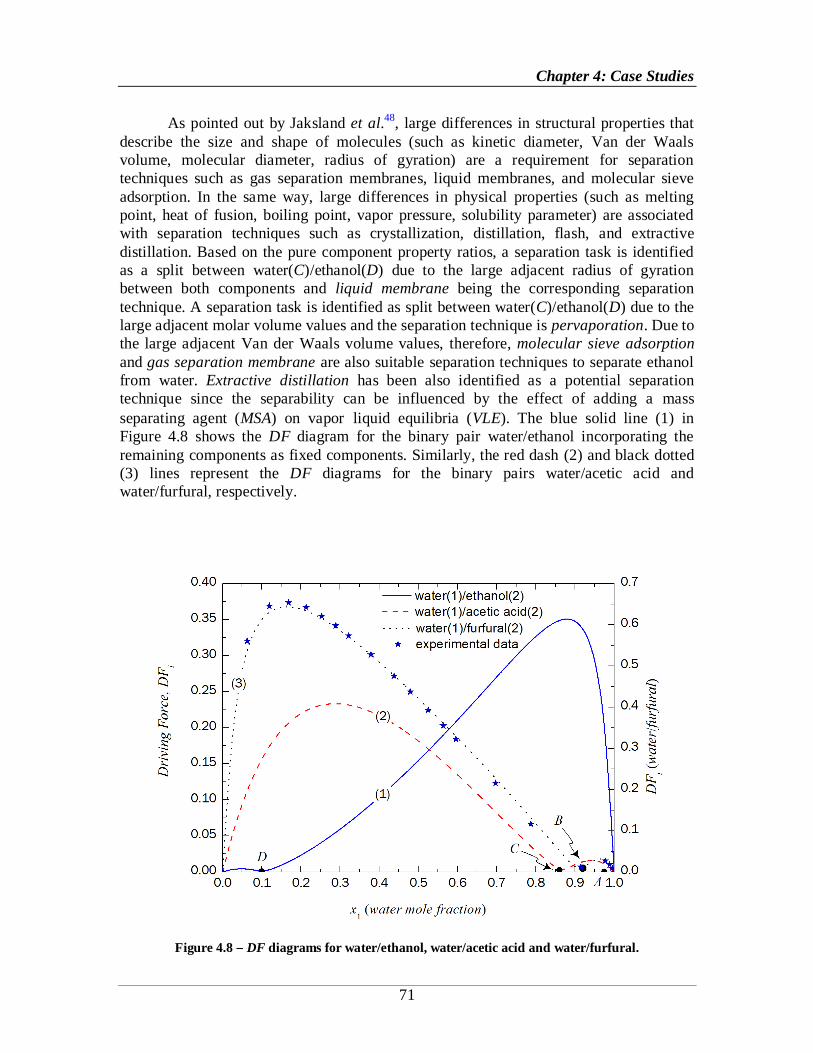
Figure 4.8 DF diagrams for water/ethanol, water/acetic acid and water/furfural. ..........71
Figure 4.9 Process group representation of the downstream separation for bioethanol
process. ....................................................................................................................................75
Figure 4.10 Solvent free DF diagram for ethanol/water mixture separation with
ethylene glycol (EG). .............................................................................................................78
Page 11
x
Figure 4.11 Solvent free DF diagram for ethanol/water mixture separation with
glycerol....................................................................................................................................78
Figure 4.12 Solvent free DF diagram for ethanol/water mixture separation with ionic
liquid ([BMIM]+[Cl] )............................................................................................................79
Figure 4.13 Solvent free DF diagram for ethanol/water mixture separation with ionic
liquid ([EMIM]+[DMP] ). ......................................................................................................80
Figure 4.14 Process flowsheet for the downstream separation using OS as entrainer....82
Figure 4.15 Process flowsheet for the downstream separation using IL as entrainer. ....82
Figure 4.16 DF diagrams for water/acetic acid, water/furfural, furfural/pyruvic acid and
water/formic acid systems......................................................................................................96
Figure 4.17 Process flowsheet for the downstream separation in the SA production
process (Rank 13). ............................................................................................................... 100
Figure 4.18 Process flowsheet for the downstream separation in the SA production
process (Rank 15). ............................................................................................................... 100
Figure 4.19 – LLE ternary phase diagrams for the system succinic acid/water/solvent. 102
Figure 4.20 – DF diagram for the ternary system succinic acid/water/solvent on a solvent
free basis. ............................................................................................................................. 103
Figure 4.21 – Solid liquid phase diagram for the binary system succinic acid/n decyl
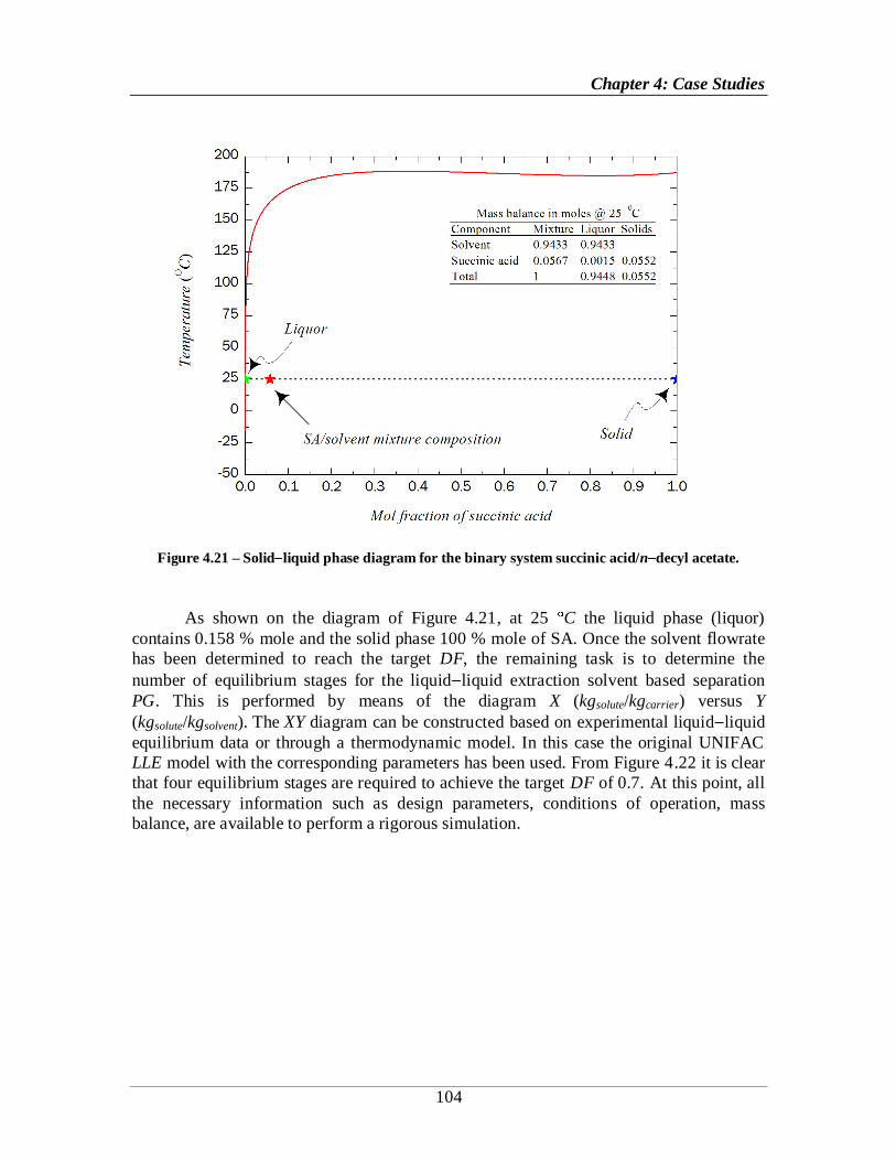
acetate. .................................................................................................................................. 104
Figure 4.22 – Graphical determination of the number of equilibrium stages for the
liquid liquid extraction based separation PG.................................................................... 105
Figure 4.23 – Solid liquid phase diagram for the binary system succinic acid/water(Lin
et al.65; Beyer
9). ................................................................................................................... 109
Figure 4.24 Process flowsheet for the DES production process (Rank 35). ................ 121
Figure 4.25 PFR trajectory in the CSA CDES space diagram where point O represents
the feed point. ...................................................................................................................... 125
Figure 4.26 Determination of AR candidate (extension through mixing solid line). ... 126
Figure 4.27 PFR and CSTR trajectories in the CSA CDES space diagram where point O
represents the feed point. .................................................................................................... 127
Figure 4.28 Determination of AR candidate (extension through mixing solid line). ... 128
Figure 4.29 Reactor configuration with feed by pass. .................................................. 128
Figure 4.30 DF diagram for binary pair ethanol/diethyl succinate. .............................. 130
Figure 8.1 Solvent free DF diagram for ethanol/water mixture separation with ionic
liquid ([EMIM]+[BF4] )...................................................................................................... 160
Figure 8.2 Solvent free DF diagram for 2 propanol/water mixture separation with ionic
liquid ([EMIM]+[BF4] )...................................................................................................... 163
Figure 8.3 Solvent free DF diagram for 2 propanol/water mixture separation with ionic
liquid ([BMIM]+[BF4] ) ..................................................................................................... 164
Figure 8.4 Schematic representation of simple liquid liquid extraction process. ....... 165
Page 12
xi
List of Tables
Table 1.1 Number of possible sequences to separate NC components by NT potential
separation techniques. ............................................................................................................12
Table 2.1 Available process groups. .................................................................................21
Table 2.2 Definition of the components in the (A/BCDE) process group. .....................26
Table 2.3 Reaction network constants and feed concentrations.......................................30
Table 3.1 Initialization of a flash process group with a 5 components synthesis
problem. ..................................................................................................................................47
Table 3.2 List of computer aided tools supporting the framework................................50
Table 4.1 Feedstock composition. ......................................................................................56
Table 4.2 Main characteristic of the base case design (anhydrous ethanol). ..................59
Table 4.3 Main characteristic of the base case design (near azeotropic ethanol). .........60
Table 4.4 Main characteristic of the base case design (non azeotropic ethanol). ..........60
Table 4.5 Main characteristic of the base case design (dilute ethanol). ..........................61
Table 4.6 List of the most sensitive indicators for the open paths (OP´s). ....................63
Table 4.7 New values of the indicators for the new process flowsheet design (with
recycle). ...................................................................................................................................65
Table 4.8 Effluent stream of the SSCF bioreactor (Alvarado Morales et al.1). .............67
Table 4.9 Pure component property ratios along with the separation techniques. ..........69
Table 4.10 Composition of the azeotropes in the process at 1 atm. .................................69
Table 4.11 Selection and initialization of a flash separation process group. .................73
Table 4.12 Final selection of the PG‟s in the synthesis problem. ....................................74
Table 4.13 Flowsheet structures of interest in the synthesis problem. ............................75
Table 4.14 Potential solvent candidates.............................................................................76
Table 4.15 Performance evaluation results for the potential solvent candidates. ...........77
Table 4.16 Ranking of the solvent candidates. ..................................................................81
Table 4.17 Mass balance results for the downstream separation (rank 3). ......................83
Table 4.18 Design parameters for the distillation columns. .............................................84
Table 4.19 Mass balance results for the downstream separation (rank 4). ......................85
Table 4.20 Design parameters for the distillation columns. .............................................86
Table 4.21 Energy consumption from rigorous simulation vs. predicted energy. ..........87
Table 4.22 Mass balance results from rigorous simulation for the downstream
separation (rank 3). .................................................................................................................88
Table 4.23 Mass balance results from rigorous simulation for the downstream
separation (rank 4). .................................................................................................................89
Table 4.24 Components involved in the SA production process. ....................................94
Table 4.25 Pure component property ratios along with separation techniques. ..............95
Table 4.26 Composition of azeotropes in the process at 1 atm. .......................................95
Table 4.27 Final selection of the PG‟s in the synthesis problem. ....................................97
Table 4.28 Flowsheet structures of interest in the synthesis problem. ............................98
Table 4.29 Mass balance results for the downstream separation. ................................. 101
Page 13
xii
Table 4.30 Mass balance results for the downstream separation. ................................. 106
Table 4.31 Design parameters for the distillation column............................................. 108
Table 4.32 Mass balance results from rigorous simulation (rank 13). ......................... 110
Table 4.33 Mass balance results from rigorous simulation (rank 15). ......................... 111
Table 4.34 Physical properties of DCM and DES. ........................................................ 114
Table 4.35 Compounds involved in the synthesis problem. .......................................... 116
Table 4.36 Pure component property ratios along with the separation techniques...... 117
Table 4.37 Composition of the azeotropes in the process at 1 atm. .............................. 117
Table 4.38 Final selection of the PG‟s in the synthesis problem. ................................. 118
Table 4.39 Flowsheet structures of interest in the synthesis problem. ......................... 119
Table 4.40 Parameters for resin catalyzed succinic acid esterification with ethanol. 122
Table 4.41 Mass balance for the reactor process group. .............................................. 129
Table 4.42 Reverse simulation results for the distillation column. ............................... 130
Table 8.1 Required properties for the simulation of the base case design. .................. 146
Table 8.2 List of compounds involved in the synthesis problems. ............................... 146
Table 8.3 Raw material and utility prices. ...................................................................... 147
Table 8.4 Reactions taking place in the pre treatment reactor. .................................... 148
Table 8.5 Reactions taking place in the ion exchange and overliming processes........ 148
Table 8.6 Production SSCF saccharification reactions. ................................................. 148
Table 8.7 Production SSCF fermentation reactions. ...................................................... 149
Table 8.8 Production SSCF contamination loss reaction. ............................................. 149
Table 8.9 Production fermentation reactions in the succinic acid process. .................. 150
Table 8.10 Pre calculated values of the reflux ratio, minimum reflux ratio, number of
stages, product purities, and driving force for ideal distillation. ...................................... 154
Table 8.11 Solvent based azeotropic separation PG overview. .................................... 157
Table 8.12 Separation task for extractive distillation using ionic liquids. ................... 161
Table 8.13 Model parameter results................................................................................ 162
Table 8.14 Model parameter results................................................................................ 162
Table 8.15 NRTL parameters. ......................................................................................... 163
Table 8.16 NRTL parameters. ......................................................................................... 163
Table 8.17 Results from the flowsheet property model vs. rigorous simulation. ........ 164
Table 8.18 LLE based separation PG overview. ............................................................ 166
Table 8.19 Crystallization separation PG overview. ..................................................... 168
Table 8.20 Pervaporation separation PG overview. ...................................................... 169
Page 14
Chapter 1: Introduction
1
1 Introduction
Process flowsheet synthesis and design are challenging tasks, which can generally
be described as follows: given a feed (raw materials) description and product
specifications, identify the process flowsheet that will allow the manufacture of the
desired product matching the given specifications and constraints. In practice, process
synthesis and design implies the investigation of chemical reactions needed to produce
the desired product, the selection of the separation techniques needed for downstream
processing, as well as taking decisions on the precise sequence of the separation unit
operations. The heat/mass integration networks to be included in the flowsheet and
finally the control strategy to be applied need to be considered as well. Furthermore, the
synthesis and design tasks also include the design of the equipment in the process
flowsheet and finally the formulation of recommendations of appropriate operating
conditions for the designed equipments.
Consequently, three types of problems can be formulated in the synthesis and
design of chemical and bioprocesses. First, process synthesis is the determination of the
process topology, i.e., the process flowsheet structure. Second, process design is the
determination of the unit sizes, the system flowrates, and the various operating
parameters of the units for a given flowsheet. Third, process optimization is the
determination of the best overall process flowsheet. Before the best system can be
developed, a suitable measure of the performance of the system must first be established.
This measure becomes the objective function for the optimization problem. These
problems can either be considered sequentially or simultaneously within the process
synthesis and design procedure to determine the final process flowsheet matching the
given specifications and constraints.
There currently exists a large wealth of literature on systematic process synthesis
and design methods for chemical processes. Excellent reviews of process synthesis are
given by Nishida et al.70
, Westerberg94
, Johns50
, and Li & Kraslawski61
. In contrast, the
same abundance of literature does not exist in the bioprocess synthesis field. Bioprocess
synthesis is often performed in a sequential fashion, proceeding from one unit to the next
until product specifications are met, and individual units are subsequently optimized to
improve plant performance. Although this approach may produce economically adequate
processes, alternative designs that are currently not explored in the bioprocess synthesis
procedures may be more profitable. On the other hand, process design in the
bioprocess based industries has made recourse to existing processes and has relied
heavily on the use of expensive pilot plant facilities in which to test out proposed new
process sequences. This has proven to be time consuming and not very systematic. As a
consequence different types of approaches have therefore been developed trying to
overcome these problems.
Page 15
Chapter 1: Introduction
2
Therefore, in this chapter a brief review of the state of the art in the synthesis and
design of chemical processes and bioprocesses is presented. Special emphasis is given to
the development of methods for synthesis and design of bioprocesses. The objectives and
the motivation behind this work as well as the general framework proposed are also
described in this chapter.
1.1 State of the Art in Chemical and Bioprocess Synthesis and
Design
In this section, different approaches to solve the synthesis and design problem,
such as methods that employ heuristics or are knowledge based, methods based on
thermodynamic/physical insights, methods based on optimization techniques, and hybrid
methods that combine different approaches into one method are described.
1.1.1 Heuristic or Knowledge based Methods
The most commonly used synthesis/design approach is the heuristic approach.
The purpose of heuristics is to narrow the list of possible processing steps based on
general experience. There are numerous examples in the literature of the use of heuristics
to solve the synthesis and design problems from the chemical industry. Particularly,
heuristics dealing with synthesis of separation processes in the chemical industry are
fairly well developed. A number of heuristic methods have been reported in the open
literature, and a brief overview is given below.
Sirrola & Rudd83
made an attempt to develop a systematic heuristic approach for
the synthesis of multi component separation sequences. In recent years, a significant
amount of work has been carried out based on this approach. The hierarchical heuristic
method is an extension of the purely heuristic approach. Seader & Westerberg81
developed a method, which combines heuristics together with evolutionary methods for
synthesizing systems of simple separation sequences. Douglas18
proposed a hierarchical
heuristic procedure for synthesizing process flowsheets where a set of heuristic rules are
applied at different levels to generate the alternatives. In this approach shortcut
calculations, based on economic criteria, are performed at every level of process design.
The process synthesis procedure decomposes the design problem into a hierarchy of
decision levels, as follows:
Level 1: Batch vs. Continuous
Level 2: Input Output Structure of the Flowsheet
Level 3: Recycle Structure of the Flowsheet and Reactor Considerations
Level 4: Separation System Specification
Level 5: Heat exchanger Network
Page 16
Chapter 1: Introduction
3
During the design process, an increasing amount of information is available at
each higher level and the particular elements of the process flowsheet start to evolve
towards promising process alternatives. Similarly, Smith & Linnhoff84
proposed an onion
model for decomposing the chemical process design into several layers. The design
process starts with the selection of the reactor and then moves outward by adding other
layers the separation and recycle system.
Barnicki & Fair4,5
developed a task oriented knowledge based expert system for
the separation synthesis problem. The design knowledge of the expert system is
organized into a structured query system, the separation synthesis hierarchy (SSH). The
SSH divides the overall separation synthesis problem into sub problems or “tasks”, which
consist of series of ordered heuristics based on pure component properties and on process
characteristics. The selector module in the knowledge based system then selects the
separation techniques for each task, based on pure component properties and on process
characteristics.
Chen & Fan12
proposed a heuristic synthesis procedure with special emphasis on
stream splitting, where only sharp separations are assumed. More recently, Martin et al.69
presented a systematic procedure based on a philosophical approach. The methodology is
based mainly on the intelligent and practical application of heuristic rules developed by
experience. The holistic methodology decomposes the original problem into four simpler
problems, namely: reaction, localization, separation and integration; the solution resulting
by solving of each problem could modify the solution resulting from problems solved
earlier or later, providing a holistic character to the methodology.
The heuristic approaches have been used in many applications, such as the
synthesis of separation systems (Seader & Westerberg81
; Nath & Motard70
), complete
process flowsheets (Siirola & Rudd83
; Powers76
), waste minimization schemes
(Douglas20
) and metallurgical process design (Linninger66
). Douglas19
illustrated, in
detail, the hierarchical heuristic method using as a case study the synthesis of benzene
through the hydrodealkylation of toluene (commonly known as the HDA process).
With respect to synthesis and design of bioprocesses, an enormous number of
heuristics originally applied for chemical process synthesis/design have also found use in
bioprocesses, namely:
1. Remove the most plentiful impurities first
2. Remove the easiest to remove impurities first
3. Make the most difficult and expensive separation last
4. Select processes that make use of the greatest differences in the properties of the
product and its impurities
5. Select and sequence processes that exploit different separation driving forces
Note that these heuristics were not developed for bioprocesses. Petrides et al.75
proposed a generalized block diagram for downstream bioprocessing shown in Figure
1.1. For each product category, (intracellular or extracellular) several branches exist in
Page 17
Chapter 1: Introduction
4
the main pathway. Selection among the branches and alternative unit operations are based
on the properties of the product, the properties of the impurities, and the properties of the
producing microorganisms, cells or tissues. Bioprocess synthesis thus consists of
sequencing steps according to the five heuristics and the structure of Figure 1.1. The
majority of bioprocesses, especially those employed in the production of high value,
low volume products are likely to operate in batch or fed-batch mode. Continuous
bioseparation processes are utilized in the production of commodity biochemicals, such
as organic acids and biofuels (ethanol, butanol).
Figure 1.1 Generalized block diagram for downstream separation (Petrides
75).
Page 18
Chapter 1: Introduction
5
1.1.2 Thermodynamic/physical Insight based Methods
Thermodynamic/physical insight based methods for synthesis and design are
those that rely on physical/chemical insights to identify feasible process flowsheets,
rather than employing heuristic or optimization methods. The insight based techniques
are thus relying on thermodynamic data of the mixture compounds in the synthesis
problem as well as the design and analysis of feasible solutions to chemical process
flowsheets.
Jaksland et al.48 and Jaksland
49 proposed a methodology for design and synthesis
of separation processes based on thermodynamic insights. Jaksland48
applies
thermodynamic insights combined with a set of rules related to physicochemical
properties rather than heuristics for selecting and sequencing the separation techniques.
This methodology is hierarchical and consists of two main levels. In the first level,
differences in component properties are calculated as ratios for a wide range of
properties. These ratios are used for initial screening among a large portfolio of
separation techniques to identify those that are feasible. In the second level, a more
detailed mixture analysis is performed for further screening. Also for separation
techniques using solvents (for instance, extractive distillation where an entrainer is
needed), these solvents are identified using a molecular design framework adapted from
Gani et al.24
. After this, in the second level suggestions for the sequencing of the
separation tasks with the corresponding separation techniques, as well as determination of
the conditions of operation are made. The methodology assumes that a knowledge base
consisting of information on pure component properties and separation techniques is
available together with methods for prediction of pure component properties (not covered
by the knowledge base) and mixture properties. Therefore, the thermodynamic
insight based methods relies on estimates of the physicochemical properties of the
components in the system.
Based on the definition of driving force (DF), as the difference in
chemical/physical properties between two co existing phases that may or may not be in
equilibrium, Bek Pedersen6, Bek Pedersen & Gani
7 and Gani & Bek Pedersen
25
developed a framework for synthesis and design of separation schemes. The framework
includes methods for sequencing of distillation columns and the generation of hybrid
separation schemes. The DF approach makes use of thermodynamic insights and
fundamentals of separation theory, utilizing property data to predict optimum or near
optimum configurations of separation flowsheets. This approach allows identifying
feasible distillation sequences as well as other separation techniques (different than
distillation).
The use of physicochemical properties information for bioprocess synthesis and
design is not a new concept. Leser & Asenjo67
defined a separation coefficient which is a
function of the physical properties difference between components and may be used to
choose between high resolution purification options. Lienqueo et al.63 developed a
Page 19
Chapter 1: Introduction
6
hybrid expert system which combines expert knowledge and mathematical correlations to
synthesize downstream purification processes for proteins. Physicochemical data on the
protein product and other proteins present (contaminants) are used to select a sequence of
unit operations to achieve the desired level of purity in the system. The selection of
separation processes is based on the quantitative values of the deviation of individual
physicochemical properties between the protein product and the contaminating proteins
(such as electrical charge as a function of pH, surface hydrophobicity, molecular weight,
and affinity) and efficiency of the separation operations to exploit this difference.
1.1.3 Optimization Methods
The problem to be solved using optimization methods can be described as
(Biegler et al.10):
Given a system or process, find the best solution to this process within a specified
set of constraints.
To solve an optimization (synthesis/design) problem, a measure of what is the
best solution is needed. Therefore, an objective function is defined for the problem,
usually a mathematical expression related to the yearly cost or profit of the process. The
result of an optimization problem is the optimal value for a set of (decision) variables,
where some of them may be bounded to lie within a defined set of constraints. A lot of
studies have been carried out on this approach, and it has been widely applied in process
synthesis and design for chemical processes. Grossmann & Daichendt32
and
Grossmann31,33
have published reviews of suitable optimization techniques for process
synthesis.
Lin & Miller64
developed a meta heuristic optimization algorithm, namely, Tabu
Search (TS), to solve a wide variety of chemical engineering optimization problems.
Tabu Search (TS) is a memory based stochastic optimization strategy that guides a
neighborhood search procedure to explore the solution space in a way that facilitates
escaping from local optima. TS starts from an initial randomly generated solution. Then,
a set of neighbor solutions are constructed by modifying the current solution. The best
one among them is selected as the new starting point, and the next iteration begins.
Memory, implemented with tabu lists, is used to escape from locally optimal solutions
and to prevent cycling. At each iteration, the tabu lists are updated to keep track of the
search process. This memory allows the algorithm to adapt to the current status of the
search, so as to ensure that the entire search space is adequately explored and to
recognize when the search space has become stuck in a local region. Lin & Miller64
highlight the approach through three chemical process examples: heat exchanger network
(HEN) synthesis, pump system configuration, and the 10sp1 HEN problem.
Angira & Babu2 developed a novel modified differential evolution (MDE)
algorithm, for solving process synthesis and design problems. The principle of modified
differential evolution (MDE) is the same as differential evolution (DE). The major
Page 20
Chapter 1: Introduction
7
difference between DE and MDE is that MDE maintains only one array. The array is
updated when a better solution is found. These newly found better solutions can take part
in mutation and crossover operation in the current generation itself as opposed to DET
(when another array is maintained and these better solutions take part in mutation and
crossover operations in the next generation) Updating the single array continuously
enhances the convergence speed leading to less function evaluations as compared to DE.
Angira & Babu2 illustrate the use of the MDE algorithm for solving seven test problems
on process synthesis and design.
Raeesi et al.78 presented a mathematical formulation of a superstructure based
solution method, and then used an ant colony algorithm for solving the nonlinear
combinatorial problem. Karuppiah et al.54
applied heat integration and mathematical
programming techniques to optimize a corn based bioethanol process. Karuppiah et al.54
first proposed a limited superstructure of alternative designs including the various process
units and utility streams involved in the ethanol production process. Short cut models for
mass and energy balances for all the units in the system are used. The objective function
is the minimization of the energy requirement for the overall plant. The mixed integer
non linear programming problem is solved through two nonlinear programming
subproblems. Then a heat integration study is performed on the resulting process
flowsheet structure.
Recently, Li et al.61 presented an environmentally conscious integrated
methodology for design and optimization of chemical processes specifically for
separation processes. The methodology incorporates environmental factors into the
chemical process synthesis at the initial design stage. The problem formulation,
considering environmental and economic factors, leads to a multi objective
mixed integer non linear optimization problem which is solved by means of a
multi objective evolutionary algorithm (a non dominated sorting genetic algorithm). Li
et al.61 highlight the application of the methodology through two case studies, the
dimethyl carbonate production process using pressure swing distillation, and an
extractive distillation process.
1.1.4 Hybrid Methods
Since application of heuristic or physical insight based methods does not seek to
obtain optimal flowsheets, while mathematical (structural optimization) techniques are
limited by the availability and application range of the model and/or the superstructure,
hybrid methods use the physical insights of the knowledge based methods to narrow the
search space and decompose the synthesis problem into a collection of related but smaller
mathematical problems. Hybrid methods are usually implemented as step by step
procedures in which the solution of one problem provides input information to the
subsequent steps in which other smaller mathematical problems are solved. Finally, such
a procedure leads to an estimate of one or more feasible process flowsheets. The final
step of hybrid methods is a rigorous simulation for verification of the proposed process
flowsheet.
Page 21
Chapter 1: Introduction
8
Hostrup41
developed a hybrid approach for the solution of process synthesis,
design, and analysis problems. The hybrid approach combines thermodynamic insights
with mathematical programming based synthesis algorithms and consists of three main
phases:
1. Pre-analysis
2. Flowsheet and superstructure generation
3. Simulation and optimization
In this way, Hostrup41
took advantage of optimization techniques to compare the
alternative synthesis routes generated by thermodynamic insights. Some other examples
of flowsheet synthesis frameworks incorporating multiple techniques are Daichendt &
Grossmann14
who combined hierarchical decomposition with mathematical
programming, while Kravanja & Glavič57
integrated pinch analysis with mathematical
programming for the synthesis of heat exchangers networks (HENs).
Based on the principles of the group contribution approach in chemical property
estimation, d‟Anterroches & Gani15
and d‟Anterroches16
developed a framework for
computer aided flowsheet design (CAFD). In a group contribution approach for pure
component/mixture property prediction, building blocks are molecular groups, whereas
for process flowsheets synthesis these building blocks, namely process groups, are unit
operations. The CAFD framework is a combination of two reverse problems; the first
problem involves the synthesis of process flowsheet structures similar to a reverse target
property estimation approach: defining the property targets for the flowsheet structure,
and then the process groups are combined based on a set of connectivity rules generating
thereby a list of feasible flowsheet structures matching the targets. The second, the
reverse simulation approach, is applied to obtain the minimum set of design parameters to
fully describe the process flowsheet from the process groups in the flowsheet structure.
By knowing the state variables of the inputs and outputs of a unit operation (i.e.,
individual molar flow rates, pressure, and temperature), through the reverse simulation
approach the design parameters of the corresponding unit operation are calculated as the
unknown variables from the process model. d‟Anterroches16
illustrates the application of
the framework with a set of case studies related to the chemical industry.
Given the particular characteristics of biological manufacturing processes such as
(Zhou et al.102):
Mixed mode batch, semi batch, continuous, and cyclic operation
Performance affected by biological variability
Highly interactive unit operations
Multiple processing steps and options
Complex feed stream physical properties
Several major obstacles arise when attempting to apply optimization methods to
solve the bioprocess synthesis/design problem. For instance, unit operations commonly
Page 22
Chapter 1: Introduction
9
used for downstream purification generally separate components non sharply, a large
selection of unit operations is available depending on the type of product (intracellular or
extracellular), biological streams are highly dilute and generally contain a large number
of compounds. Clearly, these characteristics lead to a large number of flowsheet structure
candidates and, therefore, a corresponding large search space for the synthesis algorithm.
Synthesis problems of this size are difficult to solve using numerical optimization
approaches.
The use of hybrid approaches has become a more attractive strategy to solve the
synthesis and design problem in bioprocesses. Steffens et al.87 presented a procedure for
synthesis of bioprocesses which combines the thermodynamic insights based method
developed by Jaksland et al.48,49
together with discrete programming techniques to
convert the MINLP synthesis problem into a discrete optimization problem. Stream
characteristics and unit design parameters are discretized so that all searching is
performed on discrete variables leading to a discrete optimization problem. After this,
physical property information is used to screen candidate units thereby reducing the size
of the synthesis problem. In this way, only unit operations which exploit large differences
between components in a bioprocess stream are selected. Steffens et al.87 presented two
case studies to illustrate the use of the synthesis method: the generation of process
flowsheet candidates for the downstream purification process for a protein secreted from
S. cerevisae and for the purification of an animal growth hormone bovine somatotropin
(BST).
Rigopoulos & Linke79
described the application of a general synthesis framework
for reaction and separation process synthesis to the activated sludge process design
problem the biochemical process most widely used for wastewater treatment. This
synthesis framework consists of two basic elements: a) a general modeling framework to
account for all possible design options in form of a superstructure model (includes
generic synthesis units and interconnecting streams), and b) an optimization framework
to systematically search the solution space defined by the superstructure in order to
identify targets of maximal performance and a set of designs that exhibit near target
performances.
More recently, Gao et al.28
developed an agent based system to analyze
bioprocesses based on a whole process understanding and considering the interactions
between process operations. They have proposed the use of an agent based approach to
provide a flexible infrastructure for the necessary integration of process models. The
multi agent system (MAS) consists of a number of agents that work together to find
answers to problems that are beyond the individual capabilities or knowledge of any
single agent. The MAS comprises a process knowledge base, process models, and a set of
functional agents. The proposed agent based system framework can be applied during
process development or once manufacturing process has commenced. During process
development, the MAS can be used to evaluate the design space for ease of process
operation, and to identify the optimal level of process performance. During manufacture
the MAS can be applied to identify abnormal process operation events and then to
provide suggestions to cope with the deviations. In all cases, the function of the system is
Page 23
Chapter 1: Introduction
10
to ensure an efficient manufacturing process. Gao et al.28 present a typical intracellular
protein production process to illustrate the application of the framework.
1.2 Concluding Remarks
In the previous section, a selection of methods reported in the literature for
synthesis and design of chemical and bioprocesses has been described. These methods
can in general be categorized as either heuristic or knowledge based approaches, insight
based approaches, optimization approaches, or hybrid approaches. Some of these
methods can be combined into one framework to solve the synthesis/design problem
either sequentially or simultaneously. That is, a designed process flowsheet can be the
result from the application of an insight based approach and the solution, which is not
necessarily optimal, can be used as a good initial estimate for the formulation of an
optimization problem; or when the process group concept is applied to process synthesis
to generate all possible flowsheet structures, then those most likely to be optimal with
respect to the performance criteria are selected to be further analyzed in detail using an
optimization technique. The hybrid approaches, which combine different approaches into
one method, concentrate the strategy on narrowing the search space in order to reduce the
size of the synthesis problem and to obtain near optimal solutions which deserve to be
analyzed in more detail.
The heuristic methods are often based on a limited number of operational data,
and are thus limited to only specific types of operations. If the methods are broader and
several heuristics are proposed, then they might be contradictory. On the other hand,
since the heuristic rules are based on observations made on existing processes, the
application of heuristic methods deserves careful consideration as they may lead to the
elimination of novel process flowsheets which seem to contradict prevailing experience,
yet have interesting or desirable features. Insights based methods are useful to identify
feasible separation techniques needed to perform a given separation task, as they are
based on properties of the mixture to be separated. Methods based on thermodynamic
insights such as the driving force approach are most likely to predict near optimal
solutions to the synthesis problem. Afterwards the optimization problem becomes a
straightforward task to be solved. However, if experimental data of the pure compounds
or mixture properties are not available in the open literature, the major drawback of these
methods is that they rely on the accuracy of the models and/or methods to estimate the
necessary physical properties.
Mathematical programming techniques are widely used to identify optimal
solutions for the design/synthesis problem. These solutions are based on mathematical
models of the unit operations as well as the mass and energy balances, and the optimality
of the solutions is dependent on the solver being available and the level of accuracy in
each unit operation model. In addition, a superstructure of alternative solutions needs to
be generated prior to solving the problem, and the different alternative solutions (and
combination of these) must be considered when solving the problem. In the case the
Page 24
Chapter 1: Introduction
11
optimization problem consists of only linear equations, the resulting optimization
problem is called Linear Programming (LP), and methods for solving LP problems
effectively are readily available (i.e. the simplex method). Usually, however optimization
problems for process flowsheets contain non linear equations, thereby resulting in
Non Linear Programming (NLP). In order to solve an optimization problem of this
nature certain techniques must be applied, for example reduced gradient approaches or a
Successive Quadratic Programming (SQP) method (Biegler et al.10). However, the
methods for solving NLP problems cannot guarantee that the solution found is globally
optimal, unless the objective function and the feasible region are convex.
An important part of solving a process synthesis problem is to determine which
equipment should be used in the process. If more than one flowsheet structure exists for a
particular unit operation in the process, a decision as to which flowsheet structure to use
must be made. Such decisions/selections among the flowsheet structures can be included
in the optimization problem as a vector of integer (often Boolean) variables, thereby,
implying the use of superstructures. In this case where the optimization problem consists
of linear equations and discrete variables the resulting problem is a Mixed Integer Linear
Programming (MILP) problem. But if the optimization problem consists of non linear
equations and discrete variables the resulting problem is called Mixed Integer
Non Linear Programming (MINLP) problem.
The development of a superstructure involved in the MINLP problem for process
flowsheet synthesis, is in principle, difficult. Even for the separation synthesis part of the
process flowsheet, there is a large number of process flowsheet structures to take into
account. In some cases heuristic rules can often be applied to reduce the size of the
related structural optimization problem. The size of the task/techniques selection and
sequencing problem is determined by the number of compounds (NC) in the mixture to
be separated and the number of potential separation techniques (NT) to be used in the
synthesis problem. For a separation system where all components need to be separated
from each other, Thompson & King90
proposed an expression to calculate the number of
possible sequences based on simple binary sharp splits:
12 1 !
! 1 !
NCNC
NS NTNC NC
(1.1)
Equation (1.1) has been applied for the calculation of the number of possible
sequences considering only one separation technique (NT = 1) for a different number of
compounds in Table 1.1 (column 2). As can be noticed from the Table 1.1, even when
only sharp splits and only one separation technique (i.e. simple distillation) are
considered, the number of process flowsheets in the superstructure rapidly increases with
the number of compounds in the mixture to be separated.
Page 25
Chapter 1: Introduction
12
It is clear that if the superstructure is expanded further to include, for instance,
non sharp separations, multiple processing steps and options implying more than one
separation technique to be used in the separation synthesis problem, then the size and
complexity of the problem will become immense. In addition to that, if the process
reaction is considered where for example non linear reaction models are encountered in
biocatalytic systems, the complexity of the problem will increase as well.
Table 1.1 Number of possible sequences to separate NC components by NT potential separation
techniques.
NC/NT 1 2 7 10
2 1 2 7 10
3 2 8 98 200
4 5 40 1715 5000
5 14 224 33614 140000
6 42 1344 705894 4.2E+006
8 429 54912 3.533E+008 4.29E+009
10 4862 2489344 1.962E+011 4.862E+012
20 1.767E+009 9.266E+014 2.014E+025 1.767E+028
Another important aspect that also needs to be taken into consideration is how
rigorous the models of the individual unit operations are, as it is crucial for the solution of
the optimisation problem that the models in the superstructure are consistent and correct.
Even when methods such as the Generalized Benders Decomposition (GBD) and
the outer approximation methods, are available to solve this type of problems, the
formulation of a superstructure model and solving the corresponding MINLP
optimisation problem directly are very large tasks, both mathematically and
computationally. Therefore, if the superstructure is large and detailed, it is advantageous
to screen out infeasible separation techniques through either heuristics or property
insights methods to decrease the size of the feasible region of the MINLP problem and
exploit it so as to reduce the computational costs and increase the reliability of the
solution.
Page 26
Chapter 1: Introduction
13
1.3 Motivation and Objectives
Considering the current state of the art, it is obvious that there is a lack of
methodologies to solve the synthesis and design problem in bioprocesses compared with
the development in the chemical industry which has been enormous. On the one hand,
heuristic methods are often based on a limited number of operational data and their
application needs to be considered carefully as they may lead to the elimination of novel
process flowsheets as mentioned. On the other hand, methods based on thermodynamic
insights are most likely to predict near optimal solutions. Nevertheless, their major
drawback is that they rely on the accuracy of the models and/or methods to estimate the
necessary physical mixture/pure compound properties if they are not available in the open
literature. Structural optimization frameworks have been developed for separation
synthesis, and the common focus has been primarily towards distillation sequences.
However, it is clear that the separation synthesis problem has a potential danger of
combinatorial explosion that needs to be addressed. The common strategy to be followed
is to use the existing methods and approaches to solve the synthesis problem.
Nevertheless, in some cases, this strategy has not been very successful and the synthesis
problem becomes of special concern when the portfolio of potential separation techniques
to be used in the synthesis/design problem is large as it is the case for bioprocesses. This
is often a long and cumbersome task which demands a huge computational effort.
Clearly, this is a highly undesirable situation and there is a strong need for a
systematic framework for a quick and reliable selection of high performance process
configurations. Therefore, the logical pattern to be followed is the integration of different
approaches and tools in a systematic synthesis and design framework to solve the
synthesis and design problem. This work is focused on the development of a generic
synthesis framework for chemical and biochemical processes that aims to overcome the
above limitations.
By combining different approaches in a systematic manner, a framework for
synthesis, design, and analysis of chemical and biochemical processes has been
developed in this work. The developed framework consists of five stages: 1) available
process knowledge data collection, 2) modelling and simulation, 3) analysis of important
issues, 4) process synthesis and design, and 5) performance evaluation and selection. The
framework exploits the advantages of some of the approaches described previously. For
instance, it employs the thermodynamic insights in identifying feasible separation
techniques which can be represented by a set of process groups. Then the CAFD
technique is employed through the combination of the process groups to generate only
feasible flowsheet structures. The framework is supported by a collection of computer
aided methods and tools which can help to reduce time and computational effort.
Another objective of this work is to extend the range of application of the
process group concept developed by d‟Anterroches16
in order to cover various types of
products and their corresponding processes, in particular the ones related to bioprocess
area. Therefore, a new set of process groups together with their contributions has been
developed.
Page 27
Chapter 1: Introduction
14
1.4 Structure of the Ph.D. Thesis
This thesis is organized as follows:
In Chapter 2 the theoretical background of the concepts employed in this work is
given. Concepts such as process group, driving force, attainable region and reverse
approach are explained in detail as these concepts are the core of the methods that
support the framework.
Chapter 3 gives the full picture of the developed framework for synthesis, design
and analysis of chemical processes and bioprocesses. The framework is presented in
detail together with the computer aided methods and tools supporting the framework.
Chapter 4 highlights the application of the framework through examples and
cases studies of industrial interest. The framework is highlighted with three case studies,
namely, bioethanol production process (downstream separation), succinic acid production
process, and diethyl succinate production process.
Chapter 5 gives the conclusions and lists the main contribution of this work as
well as suggestions for future directions and developments.
Page 28
Chapter2: Theoretical Background
15
2 Theoretical Background
2.1 Introduction
In this chapter the fundamental background needed for the framework for design
and analysis is described. First, a definition of the integrated synthesis, design, and
control problem is given. Then, the concepts of driving force (DF), attainable region
(AR), process group (PG) and reverse simulation are described. The DF or AR concepts
are at the core of the reverse simulation methods used in the framework. Finally,
examples highlighting the application of these concepts are presented.
2.2 Definition of Integrated Synthesis, Design and Control
Problem
Process synthesis, design, and control are three different problems that are usually
solved independently. In order to solve these problems simultaneously, it is necessary to
determine what is the common information (variables) involved in the three problems.
Many process synthesis, design and control problems deal with process variables such as
temperature (T), pressure (P) and/or composition (x). These variables are usually
regarded as intensive variables, which can be measured and based on these, other process
variables such as enthalpies, densities, volumes, and fugacities can be estimated. These
intensive variables therefore provide useful information for process synthesis, design, and
control problems, but have different functions. In process synthesis, effects of intensive
variables on the properties are determined in order to generate the process
flowsheet/configuration. In process design, optimal values of the intensive variables are
determined such that the process satisfies the specified design objectives, while in
process control, the sensitivities of the intensive variables are determined in order to
design the control system structure (i.e. determine what to control and what to
manipulate). Consequently, when the process synthesis, design, and control problems
involve the same set of variables, they can be integrated and solved as a common
problem.
2.3 Concepts
2.3.1 Driving Force (DF)
Page 29
Chapter2: Theoretical Background
16
According to Bek Pedersen6, the definition of the driving force (DF) is the
difference in composition of a compound i in two co existing phases that may or may not
be in equilibrium. As Bek Pedersen6 pointed out, this difference in composition may be
due to the thermodynamic equilibrium between the two phases as in the case of
distillation. Nevertheless, transport mechanisms other than thermodynamic equilibrium,
for instance diffusion or convection, can also promote driving forces, and therefore allow
the separation to take place.
The starting point is the availability of phase composition data, and the graphical
representation of the phase composition data (that is, plot of the DF as a function of
liquid (or vapor) composition) as shown in Figure 2.1. It can be seen that DF is a concave
function with respect to composition with a well defined maximum. Since energy needs
to be added to or removed from the system in order to create and maintain two
co existing vapor liquid phases, the value of the DF is indirectly related to the energy
added or removed. If the DF is large, less energy is involved, while if the DF is small
more energy is involved.
Figure 2.1 Driving force as function of composition.
Based on this concept, Gani & Bek Pedersen24
, Bek Pedersen6, and
Bek Pedersen & Gani7 developed a method for synthesis and design of distillation based
separation processes. With this concept, the size and relative location of the maximum
Page 30
Chapter2: Theoretical Background
17
DF is used as a design parameter for the identification of the number of stages in a
distillation column, the feed stage location, reflux ratio, etc., as illustrated in Figure 2.2.
The BDi,y and ADi,y lines represent operating lines corresponding to minimum reflux,
while BD and AD represent operating lines intersecting on the line Di,y Di,x for a reflux
greater than the minimum. Therefore, by targeting the separation task at the largest DF
value, an optimal (or near optimal) solution in terms of energy consumption is found.
Consequently, designing any type of process based on the largest DF leads to a highly
energy efficient design.
Figure 2.2 Driving force diagram with illustrations of the distillation design parameters
(Bek Pedersen6).
2.3.2 Attainable Region (AR)
Horn39
defines the attainable region (AR) as the region in the stoichiometric
subspace that could be reached by any possible reactor system. The AR is the set of all
possible output concentrations that can be obtained using the allowable fundamental
process, subject to specified constraints, for a system with specified inputs. Fundamental
processes that may be considered are physical and chemical phenomena such as mixing,
reaction, separation, and heat or mass transfer. The only element required to describe the
AR is its boundary. The objective function is usually optimized somewhere on the
boundary of the AR, as the boundary represents extremes in operation and efficiency.
Page 31
Chapter2: Theoretical Background
18
Once the AR has been found, the resulting boundary must be interpreted. The various
surfaces that comprise the boundary represent the various processing units. The
arrangement of these surfaces in the boundary determines the layout of the processing
units within the process.
In Figure 2.3 the AR in the concentration space of compounds of A and B, has
been determined for the van de Vusse91
reaction scheme. It shows that the boundary of
the AR is defined by the by passed CSTR (Constant flow Stirred Tank Reactor)
followed by a PFR (Plug Flow Reactor). More details on the construction of this AR are
provided in section 2.3.4. The important results to note are that once the boundary of the
AR has been constructed and interpreted, the best layout and the best operating conditions
with respect to the objective function can be determined. For instance, the objective
function could be to maximize the production of B given the feed conditions represented
by point O. Cost, partial pressure, temperature, selectivity, and residence time are some
other examples for possible objective functions.
Figure 2.3 Attainable region for the van de Vusse reaction (van de Vusse
91)
2.3.3 Process Group (PG)
Page 32
Chapter2: Theoretical Background
19
The process group concept (d‟Anterroches & Gani14
; d‟Anterroches15
) applies
the principles of the group contribution approach from chemical property estimation to
the synthesis and design of chemical processes. In a group contribution method for pure
component/mixture property prediction, the molecular identity is described by means of a
set of functional groups of atoms bonded together to form a molecular structure. The
process groups represent either a unit operation (such as a reactor, a distillation column,
or a flash), or a set of unit operations (such as, two distillation columns in extractive
distillation, or pressure swing distillation). The bonds among the process groups
represent the streams connecting the unit operations, in an analogous way to the bonds
combining (molecular) functional groups. For example, in Figure 2.4 (a), a simple
process flowsheet composed of a distillation column, followed by an extractive
distillation column to separate a binary azeotropic mixture by using ionic liquids as
entrainer (with the addition of a makeup of solvent), followed by a flash drum and a
stripping column to recover the solvent, could be represented with process groups.
Figure 2.4 a) Representation of a simple process flowsheet; b, c) with process groups.
Consider the process flowsheet in Figure 2.4 (a). The feed mixtures are
represented by two process groups; one inlet process group (iC), and the inlet
Page 33
Chapter2: Theoretical Background
20
process group containing two compounds (iAB). The end products are represented by
two outlet process groups (also process groups with one attachment), (oA), (oB) (a
product of purity ≥ 99.5%), and one outlet process group containing two compounds
(oBC). The two process groups representing a distillation (AB/B) and a solvent based
separation (cycB/C) have at least one inlet and one outlet stream. From the list of
available process groups a feasible flowsheet structure can be created as shown in Figure
2.4 (b/c) where a binary azeotropic mixture is separated with a downstream separation
process in which the feed mixture is concentrated up to its azeotropic point and then by a
special process group, A and B are obtained as pure products (a product of purity ≥
99.5%).
As in group contribution based molecular property prediction (where the same
molecular groups may be used to represent many molecules), the process groups are also
not component dependent, but component property dependent. Therefore, the use of the
same process groups to represent different components having similar properties is also
valid in the case of process flowsheets of a process. Note, however, that the inlet and
outlet streams (bonds) of process groups must maintain the list of components present in
them and that the path of a component through a process group establishes the flowsheet
structure. That is, process groups (A/BC) and (B/C) can be connected to form
[ (A/BC) (B/C) ] without knowing the identities of the components A, B, and C. The
identities of the chemicals (components) are only needed when the properties of the
flowsheet need to be calculated.
Currently, nineteen types of process groups are available. These are listed in
Table 2.1 and they represent the following unit operations: simple distillation column,
solvent based azeotropic distillation using organic solvents, solvent based azeotropic
distillation using ionic liquids, solvent based azeotropic distillation using hyperbranched
polymers, flash separation, kinetic model based reactor, fixed conversion reactor,
pressure swing distillation, polar molecular sieve based separation, molecular sieve
based separation, liquid membrane based separation, liquid adsorption based separation,
gas membrane based separation, crystallization, liquid liquid extraction using organic
solvents, pervaporation, simple solid liquid separation, absorption and ion exchange.
Page 34
Chapter2: Theoretical Background
21
Table 2.1 Available process groups.
Process Groups Unit Operation Process group example
Simple Distillation Column Distillation column (AB/C), (AB/BC)
Solvent Based Azeotropic Separation Extractive distillation (cycA/B)
Flash Separation Flash (fABC/BCD)
Kinetic Model Based Reactor CSTR, PFR, mixer, divider (rABC/nE/pABCD)
Fixed Conversion Reactor CSTR, PFR, mixer, divider (rABC/nE/pABCD)
Pressure Swing Distillation Distillation column, mixer, compressor, valve (swA/B)
Polar Molecular Sieve Based Separation Molecular sieve, regeneration process (pmsABC/D)
Molecular Sieve Based Separation Molecular sieve, regeneration process (msABC/D)
Liquid Membrane Based Separation Membrane (lmemABC/D)
Liquid Adsorption Based Separation Molecular sieve, regeneration process (ladsABC/D)
Gas Membrane Based Separation Membrane (gmemABC/D)
Pervaporation Based Separation Pervaporation (pervABC/D)
Crystallization Based Separation Crystallization (crsABC/D)
Liquid Liquid Extraction Based Separation Extractive column (llABC/S/SC/AB)
Simple Solid Liquid Separation Filter (e.g. belt press filter) (slAB/CD)
Absorption Absorption (abEAB/eF/EABF/EF)
Ion Exchange Separation Ion exchange column (ieABCD/ABC)
Page 35
Chapter2: Theoretical Background
22
Process group combination rules and feasible structure generation
Using the same approach as Computer Aided Molecular Design (Harper35
) it is
possible, through the process group combination rules, to generate flowsheet structures,
to evaluate them and to find the best process flowsheet matching the targets.
For instance, the process group (ABC)(DE) has three attachments: one input and
two outputs. The combination rules are as follows:
Get all the process groups matching the set of components to be
processed by the process group (ABC)(DE). There are only two
combinations: 1 input process group defined as iABCDE or a
process group with (ABCDE) as output such as (oABCDE)(oF) that will
serve as input to the process group (ABC)(DE).
Get all the process groups matching the set of componets for each output
of the process group (ABC)(DE). There are three possible combinations:
2 output process groups defined as oABC and oDE, 1 output
process group defined as oABC and one process group such as (DE) and
which will serve as input to process groups such as (D)(E) and one
process group defined as oDE and one process group such as (ABC), and
which will serve as input to process groups such as (AB)(C) or (A)(BC).
Following these combination rules and based on the definition of each
process group in the flowsheet structure ensures that the flowsheet represents a feasible
flowsheet structure.
Flowsheet property model
Similar to the situation where each molecular group in a given molecular structure
provides a contribution for a given property target (such as normal boiling point, critical
pressure, critical temperature, etc.) each process group provides a contribution to the
property of the flowsheet. This property can be the performance (in terms of energy
consumption, operating cost, profit, etc.,) defined in such a way that once the flowsheet is
described by the process groups, the flowsheet property can be calculated by means of
the corresponding flowsheet property model.
As pointed out by d‟Anterroches & Gani14
, a flowsheet property is the energy
consumption of the process flowsheet, which can be predicted by a process groups based
model where the process flowsheet is represented by process groups. d‟Anterroches15
,
has proposed the following flowsheet property model based on the driving force concept
to estimate the energy consumption for a process flowsheet involving distillation columns
with one feed stream and two product streams.
Page 36
Chapter2: Theoretical Background
23
1 1
1n NG n NG pE Q a
dfx
kk kk
k k ij
(2.1)
where Ex is the energy consumption of the flowsheet (MkJ/h for M moles/h of
feed), Qk the energy consumption of each process group, NG is the number of process
groups, df k
ij represents the maximum driving force of the process group k , ak the
contribution of the process group k . Every unit operation has a position in the flowsheet
where it can attain the theoretical maximum driving force. At any other position, the unit
operation is able to attain a lower driving force than the maximum. The topology factor
pk takes into account this fact and it is a function of the attainable driving force.
1
p Dnt
k i
i
(2.2)
Two important facts can be drawn from this flowsheet property model:
Based on driving force theory, it is clear that any process group
contribution method calculating the energy consumption (as flowsheet
property) will be component independent if it is based on the driving force
as input (known) variable, in the sense that different component binary
pairs may have the same driving force.
From the driving force diagram (see Figure 2.1), it can be observed that
driving forces can be computed for any type of two phase system as long
as the composition data of the two co existing phases are available. This
is true irrespective of whether the separation process is rate based or
equilibrium based since the driving force can be calculated from
measured or estimated composition data. Therefore, modelling/design of
separation processes based on vapor liquid, liquid liquid or solid liquid
driving forces can also be handled by the flowsheet property model in Eq.
(2.1) together with the appropriate parameter ak .
Model parameter estimation
The contributions ak of the process groups of the flowsheet property model in
Eq. (2.1) have been regressed by means of fitting experimental data. For the purpose of
this work, extractive distillation columns separating different azeotropic mixtures into
different product specifications by using novel entrainers such as ionic liquids and
hyperbranched polymers have been simulated through a validated rigorous distillation
column model. These simulation results provide a set of pseudo experimental data on the
feasibility of separation as well as the corresponding energy consumption. For the model
Page 37
Chapter2: Theoretical Background
24
parameter regression, as the driving force and the group identities are known for each
simulated task, the corresponding list of process groups is also known. Therefore, the
process group parameter ak can be estimated through regression by matching the pseudo
experimental values of Ex obtained by simulation. The following procedure is proposed
to obtain the Ex model parameter ak .
Procedure to obtain the Ex model parameters
1. Define the separation task related with the process group.
2. Construct the solvent free DF diagram for different solvent fractions,
either from experimental data or VLE calculations.
3. Perform a set of simulations for different solvent free fractions to generate
pseudo experimental data with respect to the energy consumption of the
process.
4. For each solvent fraction used in step 3, obtain the maximum df k
ij from
the solvent free DF diagram.
5. From Eq. (2.1) obtain ak parameters through the minimization of the
energy consumption of the process as shown in the objective function
given by Eq. (8.13) in the Appendix.
The detailed procedure to obtain the energy index Ex model parameters is
highlighted in the Appendix (section 8.3.1.5).
2.3.4 Reverse Simulation
Using knowledge on the state variables in inputs and outputs of a unit operation
(i.e. individual flow rates, pressure, and temperature), the reverse simulation method is
the procedure by which the design parameters of the corresponding unit operation are
calculated as the unknown variables from the process model. This methods is described
in Figure 2.5 for a simple distillation column example.
Figure 2.5 Reverse simulation overview.
Page 38
Chapter2: Theoretical Background
25
From the inlet and outlet stream definitions and the properties of the mixture in
Figure 2.5(b), the number of stages, the feed stage location and reflux ratio of the column
are back calculated as shown in Figure 2.5(a). As pointed out by d‟Anterroches15
, the
term reverse is used to highlight the difference with respect to conventional simulation.
By using conventional simulation, the design problem is solved by trial and error. Indeed,
when knowing the desired targets of a given unit operation, the design parameters are
modified or optimized to match the targets. In this case the targets are related to values of
product purities or recoveries and/or energy consumption for a separation unit such as
distillation; selectivity and/or residence time for a reaction unit. As shown in Figure 2.6,
for a simple distillation column, an initial set of design parameters is assumed first, and
then simulation is performed and the results are compared with the desired targets. If the
difference with the targets is above the acceptable error, then another set of design
parameters has to be assumed and simulation is performed again, until a satisfactory
match is found. In this section, procedures to apply the reverse simulation to a simple
distillation process group as well as a kinetic model reactor process group are presented
together with their corresponding examples.
Figure 2.6 Conventional simulation overview.
Reverse simulation procedure for the distillation process group based on the
DF concept
The procedure to determine the design parameters of a distillation column in the
distillation process group is as follows:
1. Given a distillation process group with NC components.
2. Order the components by relative volatility and identify the key components.
Page 39
Chapter2: Theoretical Background
26
3. Retrieve the maximum DF between the key components |Di MaxF , and the
composition of the light key at its maximum xD , either from experimental data or
VLE calculations.
4. Select the values of product purities or recoveries for the key components. If they
are not given use 99.5% by default.
5. If the input composition is between the requested purities for the bottom and top
products, then get the ideal number of stages Nideal for the column from the table
of pre calculated values (Table 8.10) in Appendix.
6. Set the feed plate location of the column to be F x idealN = D N1 (plate one is
the top plate of the column).
Example of reverse simulation for the distillation process group
In this section, an example of reverse simulation through the distillation
process group (A/BCDE) for the separation of a five components mixture by simple
distillation is presented. The components and the inlet composition specification are
given in Table 2.2. The relative volatilities have been calculated on the basis of the feed
composition, assuming a system pressure of 27.22 atm using the Peng Robison Equation
of State with interaction parameters set to zero.
Table 2.2 Definition of the components in the (A/BCDE) process group.
Component Flowrate
(kmole/h)
Normal
Boiling Point
(K)
Relative
volatility
Relative
volatility
between
adjacent
components
A Methane 20 111.66 358.57 6.37
B Ethane 46 184.55 56.30 3.92
C Propane 30 231.11 14.36 3.88
D Butane 3 272.65 3.70 3.70
E Pentane 1 309.22 1.00
The key components are A and B, methane and ethane, respectively. From the
driving force diagram in Figure 2.7, | 0.478Di MaxF at 0.798xD . From Table 8.10 of
pre calculated values 10idealN and 0.54minRR . Given xD and idealN , the feed plate
location is 2F x idealN = D N1 . At this stage, the distillation column is fully defined
for further rigorous simulation.
Page 40
Chapter2: Theoretical Background
27
Figure 2.7 Driving force diagram for the binary pair methane/ethane.
Reverse simulation procedure for the kinetic based reactor process group
based on the AR concept
The reverse simulation for the kinetic based reactor process group is based on the
AR concept presented in Section 2.3.2. In this section, only the attainable region analysis
is applied to the kinetic model based reactor process group. The AR concept provides a
systematic geometric method for the synthesis of chemical reactor networks (Glasser &
Hildebrandt,28
; Hildebrandt & Glasser37
). Once the AR diagram has been constructed, the
idea is to use the location of the maximum value of the desired product composition as
the basis for the reactor design to calculate other important variables such as residence
time, temperature, and reactor volume.
The kinetic model based reactor process group provides the following
information which is necessary to proceed with the attainable region analysis.
Nature of the components in the reactions.
Complete definition of the reactions and their corresponding kinetic
models.
The AR based analysis is a procedure which comprises of the following
steps:selection of the fundamental processes, selection of the state variables, definition
and drawing of the process vectors, constructing the AR, interpretation of the boundary,
Page 41
Chapter2: Theoretical Background
28
and finding the optimum for the specified objective function (operating cost, selectivity,
residence time).
1. Selection of the fundamental processes. Fundamental processes
considered in the synthesis of a reaction system are physical and chemical
phenomena such as reaction, mixing, separation, and heat and/or mass
transfer.
2. Selection of the state variables. The state of the system is characterized by
state variables. These describe the fundamental processes, but it may also
include variables from the specified objective function.
3. Definition and drawing of the process vectors. Process vectors give the
instantaneous change in the system state caused by fundamental process
occurring in that unit. For example, if only a reaction process is occurring,
the reaction vector r = r(CA, CB) will give the instantaneous direction and
magnitude of change from the current concentration position. For mixing
processes this vector gives the instantaneous change from the current state
of the system C based upon the added state C* or v(C, C*) = C C*.
4. Constructing the AR. A definite methodology to find the AR for given
fundamental processes is not available, and often a trial and error
procedure is required. Nevertheless, the AR candidate must respect the
following necessary conditions, as demonstrated by the works of
Hildebrandt & Glasser37
and Glasser & Hildebrandt28
. It is necessary that
the attainable region A with feed(s) C0 is such that:
(a) It is convex.
(b) No reaction vector on the boundary of A(∂A) points outwards
from A, that is, the reaction vectors in ∂A point inward, are tangent
to ∂A, or are zero.
(c) No reaction vector in the complement of A can be extrapolated
backwards into A.
(d) No two points on a PFR in the complement of A can be
extrapolated back into A.
It is important to point out that when using the AR technique we are
interested in constructing only the boundary of AR ( AR). Any other
interior point can be achieved by mixing points from the boundary.
Hildebrandt & Glasser37
describe a general approach for constructing the
AR. A brief description of each step is given bellow.
Step 1: Draw the PFR(s) from the feed point(s).
Step 2: Allow mixing between all the points than can be achieved
by the PFR(s). This process is known as finding the convex hull of
the curve(s).
Page 42
Chapter2: Theoretical Background
29
Step 3: Check whether any reaction vectors point out of the
surface of the convex hull. If the reaction vector points outwards
over certain regions, then find the CSTR(s) with feed points in the
convex hull that extend the AR the most. If no reaction vectors
point outwards, then check whether necessary conditions (c) and
(d) are meet. If they are not met, extend the region using the
appropriate reactor.
Step 4: Find the new, enlarged convex hull. If a CSTR lies in the
boundary at this stage, the reaction vectors must point out of the
region, and the PFR with feed points on the CSTR will extend the
region. Extend the region by finding the convex hull with these
PFR´s included.
Step 5: Repeat the last two steps, alternating between PFR‟s and
CSTR‟s, until no reaction vectors point out over the region, and
necessary conditions (c) and (d) are met.
Generally no more than four construction stages are required. The region
that we construct in this way will be attainable, but as we do not have a
complete sufficiency condition as yet, the region may not be the full AR.
We do however know that this region cannot be extended by any
combination of PFR‟s, CSTR‟s, recycle reactors and any differential
combination of reaction and mixing.
5. Interpretation of the boundary. AR analysis will not only demonstrate that
a specific output is achievable, but will also determine the process
required to achieve it, such as, mixing, reaction, separation, and heat or
mass transfer. The advantage of the geometric approach to finding the AR
is that the process layout or the operating sequence can be determined
directly from the geometry of the diagram. For a particular output of
interest there will be a path from the input to achieve the output point.
This path is interpreted in terms of the sequence of fundamental processes
required to follow the path. There is usually only one path to a particular
point on the AR boundary and an infinite number of paths to any point in
the interior on the AR region.
6. Finding the optimum. The final step is to determine the optimum for the
specified objective function. In most instances, the objective function will
be optimized at a point in the boundary due to the the fact that the
boundary points represent extremes in operation. Since the point which
optimizes the objective function has already been determined and
interpreted as a process specification and structure, the result is that the
attainable region analysis determines the best process design (the best
process layout or sequence and the best operating conditions). Also, the
sensitivity of the process design to changes in the objective function can
be tested. Since the region has already been constructed all that is required
Page 43
Chapter2: Theoretical Background
30
is to find the point that optimizes any suitable new objective function. This
point is then interpreted as the new process design.
Example of reverse simulation for the kinetic based reactor process group
In this section an example of reverse simulation for the kinetic based reactor
process group based on the AR concept is presented. The following liquid phase,
constant density, isothermal reaction network is used as example (van de Vusse91
).
1
3
2
k k
kA B C (2.3)
42 kA D (2.4)
The initial characteristics of the reaction network are shown in Table 2.3. The
problem consists of finding the best reactor network that maximizes the amount of
product B for a feed of pure A. The desired product B is formed from A via a reversible
reaction from A, and is consumed by a consecutive irreversible reaction to C, and is also
in competition with the by product D.
Table 2.3 Reaction network constants and feed concentrations.
Parameter Value Units
1k 0.01 1 s
2k 5 1 s
3k 10 1 s
4k 100 3m kmoles
Feed concentrations Value Units 0
AC 1 3kmole m
0 0 0
B C DC C C 0 3kmole m
In this particular example, as fundamental processes mixing, perfectly mixed
reaction (CSTR) and reaction with no mixing (PFR) are considered. The mass balance
equations for a PFR are:
2
1 2 4A
A B A
dCk C k C k C
d (2.5)
Page 44
Chapter2: Theoretical Background
31
1 2 3B
A B B
dCk C k C k C
d (2.6)
3C
B
dCk C
d (2.7)
2
4D
A
dCk C
d (2.8)
The mass balance equations for a CSTR are:
0 2
1 2 4A A A B AC C k C k C k C (2.9)
0
1 2 3B B A B BC C k C k C k C (2.10)
0
3C C BC C k C (2.11)
0 2
4D D AC C k C (2.12)
The state variables for this example are AC and BC . Firstly, BC is a state variable
because it is its value that we wish to optimize. AC is a state variable because, looking at
the right hand side of Eqs. (2.5) (2.12), the behavior of BC is entirely dependent on the
change in AC . is not a state variable because it is the independent variable in the
system.
Before moving further into the analysis, it is useful to determine the dependence
of species concentrations as function of residence time. For a PFR, this is determined by
numerically solving the mass balances in Eqs. (2.5) (2.8), giving the concentration
profiles of AC and BC in Figure 2.8. Similarly, the set of mass balance Eqs. (2.9) (2.12)
can be solved to give the locus for the CSTR as is varied, provided in Figure 2.9.
Page 45
Chapter2: Theoretical Background
32
Figure 2.8 Concentration profiles as a function of space time for a PFR. Note that profiles for CC
and CD are not shown.
Page 46
Chapter2: Theoretical Background
33
Figure 2.9 Concentration profiles as a function of space time for a CSTR. Note that profiles for CC
and CD are not shown.
With this information we can plot a state space diagram B AC C , as shown in
Figure 2.10.
Page 47
Chapter2: Theoretical Background
34
Figure 2.10 State space diagram. Point O represents the feed point.
It may be seen that a PFR gives a somewhat higher concentration of B at AC
around 0.15 ( 0.85), while CSTR gives an optimum concentration of B at AC around
0.3 ( 0.70). Thus, taking into account the performance of ideal reactors it comes out
that a PFR is preferred. Now the question is wether we can find a better reaction system.
The construction of the AR can provide the answer to this question.
4. Constructing the AR
Step 1: Draw the PFR from the feed point. Alternatively, the
trajectory of the reaction in the B AC C space of the PFR can be
drawn directly from the relation:
1 2 3
2
1 2 4
B A B B
A A B A
dC k C k C k C
dC k C k C k C (2.13)
In others words, the tangent to the reaction trajectory of species B and
A in PFR is given by the ratio of the corresponding rates, as shown in
Figure 2.11.
Page 48
Chapter2: Theoretical Background
35
Figure 2.11 State space diagram for PFR.
Step 2: Finding the convex hull of the curve. As the PFR region is
not convex, the full correction to convexity can be obtained by
building what could be called a “convex hull”. This can be done
graphically by means of the segment OX. It can be observed that a
point on the segment OX represents a PFR with by pass, the
position depending on the fraction of feed split (see Figure 2.12).
Page 49
Chapter2: Theoretical Background
36
Figure 2.12 Determination of AR extension through mixing process (solid line).
Summing up, we have obtained a candidate AR. This obeys the
first three conditions, because it contains the feed, and it is convex.
The question is if it also satisfies the fourth condition? The answer
is no. Indeed, we have seen that a CSTR starting from the feed
gives a better selectivity than a PFR. Thus, a CSTR should be
considered firstly.
Step 3: Draw the CSTR from the feed point. It can be seen in
Figure 2.13, when PFR and CSTR trajectories start from the same
feed point, there is a large overlap in the behavior of the two
reactors. However, CSTR gives a better selectivity at lower
conversion, while PFR gives a higher selectivity at higher
conversion. We proceed as before adding a convex hull at the right
of the CSTR region, starting with the feed point. This can be done
by drawing the tangent OP, as indicated in Figure 2.13.
Page 50
Chapter2: Theoretical Background
37
Figure 2.13 Determination of AR extension through mixing process (solid line).
In fact, the vector OP represents a CSTR, due to the relation:
0 2
1 2 4
01 2 3
B B A B A
A B BA A
C C k C k C k C
k C k C k CC C (2.14)
Points on the line represent a CSTR with by pass, where the ratio of
the direct feed and by pass is found by means of the Lever Arm Rule.
Step 4: Finding the new convex hull. From Figure 2.13, it can be seen
that the region at the left of the point P is not convex. We can keep on
extending the region from the point P with a PFR, as indicated in
Figure 2.14. The computation is performed by simply integrating the
differential equations of the PFR but this time input concentrations are
supplied by the exit of the CSTR. The new augmented region is
convex. This time all the four conditions are fulfilled. No other mixed
reactors can be found above the boundary that could give a higher
amount of B. Therefore, the solid line corresponds to the final AR.
Page 51
Chapter2: Theoretical Background
38
Figure 2.14 Resulting AR candidate.
5. Interpretation of the boundary
After obtaining the AR, in fact by only drawing its boundary, the synthesis of the
reaction network is easy. Figure 2.15 shows possible configurations. For instance, up
to 60% conversion a single CSTR with by pass gives the best selectivity. The highest
selectivity of all the reaction systems is obtained with a combination CSTR PFR.
The graphical construction gives the intermediate conversion, and enables us to
determine the size of the two reactors. The CSTR has to be sized to reach a
conversion of 60%, followed by a PFR to complete the reaction up to 78%.
Hence the combination CSTR PFR gives a higher yield in B than that could be
obtained with either a single CSTR or PFR, as well as with other CSTR or PFR
arrangements, in series or parallel. In general, the proposed configuration is the best
combination of the all imaginable combinations of CSTR and PFR reactors. The last
result is important, and illustrates the power of the AR approach. Now we are sure
that a better reactor configuration cannot be obtained, and the search for other
systems is not necessary.
Page 52
Chapter2: Theoretical Background
39
Figure 2.15 Possible configurations for the reactive system.
6. Finding the optimum
The final step is to determine the optimum for the specified objective function. In this
case, the objective function is to maximize the production of B given the feed of 1
kmole/m3 of A. It can be seen easily from Figure 2.15 that a maximum of 1.24x10
4
kmole/m3
of B can be achieved using a CSTR with effluent concentration of A of 0.4
kmole/m3 followed by a PFR with an effluent concentration of A of 0.18 kmole/m3
.
The corresponding residence time of the CSTR and the FPR are 0.037 s and 0.031 s
respectively.
2.4 Discussion
In this chapter, driving force (DF), attainable region (AR), process-group (PG),
and reverse simulation concepts have been described. The idea behind of the reverse
simulation concept is that the solution (target) for a given design problem is known in
advance. As in a reverse simulation method the entire space of feasible solutions to the
design problem is determined a priori. Therefore, it is immediately known if the solution
(our target) exists or not, and if it exists, if it is also feasible or not. In this way the
conventional procedure of trial an error is avoided. Nevertheless, the reverse simulation
Page 53
Chapter2: Theoretical Background
40
method does not guarantee that the design will be the final optimal design, but it does
guarantee that the design will match the constraints and will be a feasible design. With
regard to the PG concept, the range of application relies on having a set of
process groups representing all types of unit operations as well as suitable property
models for each type of unit operation. One important feature of the PG concept itself is
that the PG´s are not component dependent, but component property dependent.
Therefore, the ability to use the same PG with different components having similar
properties is exploited such as it is in a group contribution based molecular property
prediction method. By means of the CAMD techniques, but using PG´s like building
blocks to generate flowsheet structures, the entire solution space is determined.
Afterwards, the solution space is reduced through screening with performance criteria,
and only the most promising flowsheet structures according to the performance criteria
can be selected to be analyzed in more detail.
Page 54
Chapter 3: Framework for Design and Analysis
41
3 Framework for Design and Analysis
3.1 Introduction
In this chapter, first the proposed framework for design and analysis of chemical
and biochemical processes is presented together with its workflow and the various tools
used in the different calculation stages. Each stage is described in detail pointing out the
main goals to be achieved at each calculation stage of the framework. Second, since one
of the supporting methodologies at stage four of the framework is the process group
contribution methodology (PGC) which in turn is supported by various computer aided
tools and methods It is also presented in detail together with its workflow. Third, a
description of ICAS (Gani et al.23; Gani
26), the Integrated Computer Aided System
developed at CAPEC (Computer Aided Process Engineering Center) is also given. This
software package integrates the methods and tools used in the framework to assist the
user in the resolution of product/process engineering problems. A list of the tools used at
different stages of the framework is given together with a brief description of them.
3.2 Overview of the Framework
The proposed framework for design and analysis of chemical and biochemical
processes consists of five stages, and its workflow together with the supporting tools and
methods at each stage is outlined in Figure 3.1. Stage 1 involves a pre analysis of the
product qualities and its characteristics which will define the process needs. The
objective of this stage is to establish a base case design to manufacture the product. In
stage 2, the objective is to evaluate the base case design and generate information for
further analysis. This additional information is generated by performing mass and energy
balances on known production process steps through process simulation. The information
generated in stage 2 is analyzed in stage 3 to identify bottlenecks and/or critical points
where the base case design can be improved. Based on the identification of these
bottlenecks, targets for further improvements are defined. It is worth pointing out that the
starting point is a reference (or known) design of a process. In stage 4 design candidates
are generated that match the targets defined in stage 3. Finally, in stage 5, the most
promising design candidates are verified through rigorous simulation and the most
promising one is selected based on suitable performance criteria. The performance
criteria chosen depends on the goal of the synthesis/design problem to be solved. In the
following sections each one of the five stages of the framework is described in detail.
Page 55
Chapter 3: Framework for Design and Analysis
42
3.2.1 Stage 1 Available Process Knowledge Data Collection
As the starting point is a base case design, in general, the minimum amount of
knowledge needed for the production route should be the data needed to perform the
modelling and simulation in stage 2. Some of the data, if not available from literature or
from experiments, could be generated via predictive software. For example, the
properties of identified chemicals, and conversions of reactants/substrates (if the
corresponding kinetic models are available) could be predicted. These data are important
because they affect the energy and water demand for the process operations. Therefore,
the availability of accurate values for properties such as heats of reaction, vapor
pressures, heats of vaporization, heat of formation to mention some, for example, are
extremely important.
Figure 3.1 Workflow diagram of the framework for design and analysis.
3.2.2 Stage 2 Modelling and Simulation
Page 56
Chapter 3: Framework for Design and Analysis
43
Analysis of any process requires data. In this case, the necessary data are related
to the production steps of each operation. These data could be available in the form of
measured plant data. However, not all necessary data are usually available, especially not
in the process design phase, and even if they do, a check of the data for consistency is
typically necessary. Another option for generating data is to perform mass and energy
balances on the known production steps. This can be easily done through process
simulation if all necessary models are available in the selected process simulator. In this
thesis, we are only dealing with steady state/analysis and therefore, the necessary
modelling/simulation tools correspond to steady state simulation. Several options for
modelling and simulation exist and for reasons of availability and ease of use, the PROII
simulator supported by ICAS tools (Gani et al.23; Gani
26) has been used for process
simulation. PROII (PROII77
) is a steady state simulator, while ICAS tools (Gani et
al.23; Gani
26) is a collection of tools for property prediction (ProPred, for prediction of
missing pure component properties), modelling (MoT, to generate missing models)
thermodynamic property model analysis (TML, for property model analysis and
parameter estimation) and design (PDS, for design of separation processes based on DF).
More details on the ICAS tools (Gani et al.23; Gani
26) are provided in Section 3.4.
3.2.3 Stage 3 Analysis of Important Issues
Based on the generated data, the objective here is to establish the process points
where improvements can be made, without trade off or compromise. The improvements
can be related to reduction of waste, cost, energy consumption, and/or environmental
impact. If the goal is to generate a more sustainable process, the method used is the
indicator based design and analysis of Carvalho et al.11. The corresponding
computational tool is SustainPro, which is able to generate, screen, and then identify
sustainable alternatives in any chemical process by locating the operational,
environmental, economic, and safety related bottlenecks inherent in the process. If the
goal is to improve the performance of a process flowsheet in terms of its operational cost
and/or energy consumption, a techno economic analysis is performed to identify those
process areas with a high potential for improvement.
3.2.4 Stage 4 Process Synthesis and Design
Once the targets have been defined, the objective of stage 4 is to generate design
candidates matching these targets. The focus in this stage is to improve the performance
of a process flowsheet in terms of its energy consumption and/or sustainability. For the
synthesis and design of more efficient processes in terms of energy consumption the
process group contribution (PGC) methodology to generate design candidates is used.
Full description of the PGC methodology is provided in Section 3.3 along with its
workflow.
Page 57
Chapter 3: Framework for Design and Analysis
44
3.2.5 Stage 5 Performance Evaluation and Selection
The most promising design candidates are identified based on suitable
performance criteria. The performance criteria chosen depend on the final goal of the
design problem to be solved. If the performance criteria is the energy consumption of a
process flowsheet, the PGC methodology is used to perform the evaluation with the
corresponding flowsheet property model. For the identification of sustainable design
candidates, the sustainability metrics defined by the Institution of Chemical Engineers by
Azapagic3 can be used.
3.3 PGC Methodology Overview
The PGC methodology relies entirely on the process group concept presented in
Chapter 2. Based on the PG concept d‟Anterroches15,16
proposed the PGC methodology
which consists of the following steps: (1) synthesis problem definition, (2) synthesis
problem analysis, (3) process group selection, (4) generation of flowsheet candidates, (5)
ranking/selection of flowsheet candidates, (6) reverse simulation, (7) final verification. In
the following sections a detailed description of the PGC methodology is provided
together with the different methods and tools supporting the methodology.
Page 58
Chapter 3: Framework for Design and Analysis
45
Figure 3.2 Workflow diagram of the PGC methodology.
3.3.1 Step 1 Synthesis Problem Definition
This step involves two tasks as objectives: i) the definition of the structural
constraints, which are related to the definition of the raw materials (inputs) and desired
products (outputs) of the process flowsheet and ii) the selection of the flowsheet property
model. As inputs and outputs are represented by input and output process groups,
respectively, then the remaining task is to determine the correct sequence of unit process
Page 59
Chapter 3: Framework for Design and Analysis
46
operations represented by process groups that will manufacture the desired product
matching the flowsheet property target as well as the product purity.
3.3.2 Step 2 Synthesis Problem Analysis
The objective here is to generate information for the subsequent steps. This step
involves two tasks: i) reaction analysis and ii) pure component/mixture property analysis.
i) The reaction analysis is performed with the objective of identifying the reaction tasks
needed to produce the desired product. Then, a database search is performed to find the
chemical reaction or set of chemical reactions yielding the desired product. ii) The pure
component/mixture property analysis is performed by means of the thermodynamic
insights based method developed by Jaksland et al.48 and Jaksland
49. This method is
based on the principle that the differences (or property ratios) in the values of properties
among the components of the mixture to be separated can be exploited by the
corresponding separation technique. Therefore, the pure component/mixture property
analysis is performed with the objective of retrieving information related to the feasible
separation technique to be used in the synthesis problem.
3.3.3 Step 3 Process Group Selection
The selection of the process groups is based on analysis of the synthesis problem.
It is worth pointing out that according to the process group concept (see Chapter 2,
Section 2.3.3), a process group is component property dependent. It means that a given
process group can be used for different sets of components as long as the properties are
matched. The procedure to follow is to retrieve the process groups from the PG‟s
database (Table 2.1) which match with the separation techniques identified in the
previous step. This step involves two tasks: i) selection and initialization of reaction
process groups and ii) selection and initialization of separation process groups. The
initialization of a process group is obtained through a procedure where a process group
is associated with a given set of components.
i). Selection and initialization of reaction process groups: From the synthesis
problem analysis, the complete list of reactions, kinetic model parameters or
conversion rates are available. For each reaction (or set of reactions) if the
kinetic model parameters are available, a kinetic model based reactor
process group is selected; otherwise a fixed conversion based reactor
process group is selected. As the corresponding reaction process groups are
selected, they are initialized with the components involved in the chemical
reaction (or set of reactions).
ii). Selection and initialization of separation process groups: The separation
process groups are selected based on the identified separation techniques
during the synthesis problem analysis. For each feasible separation technique
Page 60
Chapter 3: Framework for Design and Analysis
47
identified in the synthesis problem analysis, the corresponding process group
is selected. The selected process group can be initialized with different sets of
components, if each set is matching the property dependence of the
process group.
Consider a mixture of five components labeled as A, B, C, D, and E in the
synthesis problem. Based on their vapor pressure and boiling point ratios, a feasible
separation task is identified between components B and C. The corresponding separation
technique associated to this set of properties is flash separation and the process group
representing this separation technique is the flash separation process group. Therefore,
the flash process group can be initialized with four different sets of components as
shown in Table 3.1. This is based on the assumption of an ideal system, where no binary
azeotropes exist, and assuming that the components are ordered according to decreasing
relative volatility.
Table 3.1 Initialization of a flash process group with a 5 components synthesis problem.
Components in the synthesis problem A, B, C, D, E
Separation task B/C
Property dependence Vapor pressure, boiling point
Separation technique Flash separation between B and C
Matching set of components
5 4 3 2
(ABCDE) (ABCD) (ABC) (BC)
(BCDE) (BCD)
Initialized process groups (fAB/CDE) (fAB/CD) (fAB/C) (fB/C)
(fB/CDE) (fB/CD)
After initialization, each separation process group is ready to be used in the
generation of flowsheet structures. All the initialized flash separation process groups are
grouped in the pool of process groups used during the synthesis of the flowsheet
structures.
3.3.4 Step 4 Generation of Flowsheet Candidates
The objective in step four is to combine the process groups selected in step three
according to a set of connectivity rules and specifications proposed by d‟Anterroches &
Gani15
and d‟Anterroches16
to generate flowsheet structures. Each process group has
outlet specifications, which are guaranteed to be met if the connectivity rules of the
process group are satisfied. The output specifications are based on mass balance rules.
For instance, consider the case of the separation of a mixture of three components labeled
A, B, and C into three pure products using only one separation technique, in this case
simple distillation. This leads to two possible configurations, which are represented
through simple distillation process groups, as shown in Figure 3.3. The feed mixture is
Page 61
Chapter 3: Framework for Design and Analysis
48
represented by an inlet process–group iABC (groups with one attachment). The end–
products (groups with a single attachment) are outlet process–groups, such as, oA, oB, oC
(a pure product with at least 99.5% purity) or oAB, oBC (a mixture product). An
intermediate product (groups with two or more attachments) is defined as a product
resulting from one unit operation such as (AB) or (BC) which in turn serves as an inlet
stream for a subsequent unit operation, such as (A/B) or (B/C), respectively (see Figure
3.3).
Figure 3.3 Process–group flowsheet representation of two configurations in the separation of a
three component mixture into three pure streams.
The process–groups guarantee the recovery of the components in their outlets
during the generation of the flowsheet structures. For instance, the process–group (A/B)
can be connected to the output of process–group (AB/C) independently of the
composition of the mixture of A, B, and C entering the (AB/C) process–group. In this
case, the outputs of the process–group (AB/C) are ensured to be on the one hand a
mixture of A and B, and, on the other hand, a stream with a high purity and recovery of
component C. Summarizing, a process–group is flexible in its inputs and strict in its
outputs. Based on this analysis, the connectivity rules and specifications for the simple
distillation process group are as follow:
The simple distillation process group consists of one inlet and two outlet
process groups.
The inlet connection process group must contain the exact same components
as the ones set during the initialization procedure.
The two outlet connection process groups are ensured to have at least 99.5%
purity in pure streams and above 99.5% recovery of key components if
mixtures. The outlet pressure for both outlets is set to the process group
operational pressure and the temperature is set to the bubble point of the
mixtures. The assumption is made that there is no pressure drop in the
column.
As mentioned above, each process group has its connectivity rules as well as
outlet specifications, which can be found in d‟Anterroches16
. For the new set of
Page 62
Chapter 3: Framework for Design and Analysis
49
process groups developed in this thesis, the complete details are presented in the
Appendix.
3.3.5 Step 5 Ranking/Selection of Flowsheet Candidates
The generated flowsheet structure candidates are tested with respect to their target
property values chosen in step one, using the corresponding flowsheet property model.
Currently, there are available property models to assess the performance in terms of
energy consumption for distillation process groups, flash process groups, solvent based
distillation process groups using three types of entrainers (organic solvents, ionic liquids,
and hyperbranched polymers) and pressure swing distillation. The flowsheet property
model for these process groups is based on the DF theory presented in Section 2.3.1 of
Chapter 2.
3.3.6 Step 6 Reverse Simulation
The reverse simulation step involves two tasks: i) the resolution of the mass
balance through each process group in a process flowsheet and ii) the calculation of the
flowsheet design parameters of the process unit operations through reverse simulation in
the flowsheet structure.
The mass balance is performed through each process–group present in the
generated flowsheet option. The operating conditions such as pressure and temperature of
the outlet streams are given by the process–group definition. For instance, in the case of
distillation process–groups, recovery of the components lighter than the light key is equal
to 100% in the overhead product and the recovery of the components heavier than the
heavy key is equal to 100% in the bottom product. The recovery of the key components is
greater than or equal to 99.5%. The resolution of the mass balance can be performed by
means of any commercial simulator.
The reverse simulation procedure for separation process groups (such as
distillation, extractive distillation, flash) is based on the DF concept and it has been
described in Section 2.3.4 of Chapter two. The kinetics based reactor process group
employs the identified highest point in the AR diagram and using this point
(reactant product concentration) as the reference, calculates all other reactor design
parameters as has been described in Section 2.3.4 of Chapter two.
3.3.7 Step 7 Final Verification
At this step of the methodology, all the necessary information to perform the final
verification through rigorous simulation is available. The use of rigorous simulators like
PROII (PROII77
) to further refine the most promising process flowsheet and to perform
optimization of the design parameters is used in this step.
Page 63
Chapter 3: Framework for Design and Analysis
50
3.4 Computer Aided Tools in the Framework
3.4.1 ICAS Integrated Computer Aided System
In the proposed framework various computer aided tools are used, which are part
of the Integrated Computer Aided System (ICAS) (Gani et al.23; Gani
26). ICAS is a
package of programs and tools communicating with each other to assist an engineer in the
resolution of product/process engineering problems. A list of tools used at different
stages of the framework is given in Table 3.2.
Table 3.2 List of computer aided tools supporting the framework.
Supporting tool Purpose Stage
ICAS CAPEC DBM Retrieval of pure component
and mixture properties. 1
ICAS ProPred Prediction of pure component
properties based on GC methods. 1
PROII Process simulation
and optimization. 2, 4, 5
SustainPro Process analysis
(identification of bottlenecks). 3,4
ICAS TML VLE, LLE calculations. Estimation
of thermodynamic model parameters. 1, 4
ICAS utility toolbox VLE, LLE and SLE diagrams.
Separation efficiency diagrams (DF diagrams). 1, 4
SMSWin VLE, LLE and SLE calculations. 1, 4
ICAS ProCAFD Computer aided tool for process synthesis
and design. 4
ICAS ProCAMD Computer aided tool for molecular and mixture
design; used for solvent design. 4
ICAS PDS Design and synthesis of distillation based
separation schemes. 4
3.4.1.1 ICAS CAPEC Database Manager (DMB)
The framework for design and analysis requires information related to the
physicochemical properties of the compounds for a given synthesis/design problem.
Therefore, use of a database for properties of chemicals is essential. The CAPEC
database includes collected and screened experimental data of pure component properties
for approximately 13200 pure compounds, mixture data and solubility data from the open
Page 64
Chapter 3: Framework for Design and Analysis
51
literature. A very important feature of the CAPEC database manager is that it allows to
the user to add new compounds together with their property data in user defined
databases. Unless otherwise stated, all properties of compounds used in this thesis were
retrieved from the CAPEC database.
3.4.1.2 ICAS ProPred: Property Prediction Toolbox
When the properties of specific compounds either do not exist in the CAPEC
database or experimental data are not available in the open literature, a computational
tool for the prediction of pure component properties is required. Before moving forward,
it is necessary to predict the properties of these compounds before they can be added to
the database and be used in the solution of a given problem. ICAS ProPred is a tool
integrated into ICAS directly for property prediction of pure component properties.
ICAS ProPred is an interactive program, where the user can draw a molecule in a
graphical interface by connecting fragments of molecules such as CH2, CH3, OH, etc,
into feasible molecules. Currently the software can predict properties using four methods
Marrero & Gani68
, Constantinou & Gani13
, Joback & Reid50
, and Wilson & Jasperson97
.
CI MG and Van Krevelen group contribution methods (Satyanarayana & Gani80
) are
used for polymer property prediction. ICAS ProPred was used in this work to calculate
properties of the compounds when they could not be found in the available databases and
other sources did not contain the needed property value.
3.4.1.3 ICAS TML: Thermodynamic Model Library
ICAS TML is used for three purposes. Firstly, it was used for advising which
thermodynamic model should be used in process simulations for given composition
ranges of compounds present in the mixture and the condition ranges (e.g. range of
temperature and pressure). This implementation is based on the methodology presented
by Gani & O‟Connell22
. Secondly, with ICAS TML it is possible to obtain mixture
properties like bubble and dew points, PT flash (multi phase), etc. Last but not least,
when the selected thermodynamic model exhibits unsatisfactory deviations from
experimental data, it is possible to “fine tune” the thermodynamic model parameters
with ICAS TML. In this thesis ICAS TML has been used for two purposes: for the
selection of the thermodynamic model and for estimation of the parameters of the
selected thermodynamic models based on available experimental data.
3.4.1.4 ICAS PDS: Process Design Studio
The Process Design Studio (PDS) is used in this thesis to design the distillation
columns. An important feature of this tool is the analysis of the feasibility of achieving a
specified distillate or bottom product composition from a specific feed, by manipulating
the reflux ratio. In the distillation design part of PDS, given the identity of the mixture
Page 65
Chapter 3: Framework for Design and Analysis
52
compounds, the thermodynamic model, the desired product compositions and reflux, the
program returns the number of stages and the feed stage location. Moreover, ICAS PDS
can also be used to compute binary and ternary azeotropes, phase diagrams, distillation
boundaries, and residue curve maps. In this way, it can be used for preliminary analysis
of a mixture to be separated by distillation. In this thesis, ICAS PDS has been used for
design verification of separation processes.
3.4.1.5 ICAS ProCAMD: Computer Aided Molecular Design
ICAS ProCAMD is based on the multi level computer aided molecular design
technique developed by Harper & Gani37
. It can be used for various types of molecular as
well as the mixture design problems. Each problem can defined in terms of six main
categories, represented by a page in the problem setup menu. The six categories are: (1)
general problem control, (2) non temperature dependent properties, (3) temperature
dependent properties, (4) mixture properties, (5) azeotrope/miscibility calculations and
(6) biodegradation calculations. The generated molecules can be listed and ordered
according to different target (desired) properties, and are highlighted if they are present in
the CAPEC database. In this thesis ICAS ProCAMD has been used only when selection
or replacement of solvent was required in stage four of the framework.
3.4.1.6 ICAS ProCAFD: Computer Aided Flowsheet Design
ICAS ProCAFD is the computational implementation of the computer aided
flowsheet design framework (CAFD) developed by d‟Anterroches and Gani15
. In the
same way that ProCAMD is used to design molecules by combining molecular groups,
ProCAFD generates flowsheet structures by means of the combination of PG’s for a
given problem specification (e.g. defined in terms of available raw materials and desired
products). The generated flowsheet structures are then ranked based on performance
criteria. Finally, the user chooses the most promising one for further analysis. It is
applicable to a wide range of problems as long as the process groups as well as the
flowsheet property model needed to represent and assess the flowsheet structures
respectively are available. In this thesis ProCAFD is used to generate flowsheet structures
in stage four of the framework.
3.4.2 SustainPro
SustainPro is an EXCEL based software developed by Carvalho et al.11
, which is
able to generate, screen, and then identify sustainable alternatives in any chemical
process by locating the operational, environmental, economic, and safety bottlenecks
inherent in the process. The input data needed to use SustainPro are the reference (base
case design) design/operational data of the process (mass flows, energy flows and
costs). The data from PROII (PROII77
) steady state simulations are exported to an excel
Page 66
Chapter 3: Framework for Design and Analysis
53
sheet. This excel sheet is then imported to SustainPro. In addition, the user needs to
provide data for the calculation of safety indices, such as flammability, explosiveness,
and toxicity limits of all the compounds involved in the process. SustainPro first performs
a flowsheet decomposition based on identification of component mass and energy
“paths” (open and closed paths). It then calculates a set of mass and energy indicators
(Carvalho et al.11) that trace the paths of the component “mass flows” and
“energy flows” as they enter and leave the process (they may also be generated or
consumed within the process). Following this, the SustainPro software identifies the
critical points the ones that allow the best improvements in the process through
sensitivity analysis. In this way the target indicators are selected and local sensitivity
analysis is subsequently performed to determine the design and the operational
parameters that influence the targets.
3.5 Discussion
A systematic methodology for synthesis/design and analysis supported by
computer aided methods and tools can help to reduce time and man power resources. In
this chapter, a framework for synthesis and analysis of chemical and biochemical
processes together with the computer aided methods and tools have been presented.
Within this framework, emphasis is given to the PGC methodology, which is used to
generate and test feasible design candidates based on the principle of the
group contribution approach used in chemical property estimation. As pointed out by
d‟Anterroches15
the three fundamental pillars of the PGC methodology are the
process groups (building blocks), connectivity rules to join the process groups and
flowsheet property models to evaluate the performance of the flowsheet structures.
Therefore, through the addition of new process groups the application range of the PGC
methodology can be further extended. With respect to the PGC methodology, some
aspects deserve the following remarks:
The flowsheet property model is truly predictive and component independent,
this means that different component binary pairs may have the same DF.
The combination of the process groups to form flowsheet structures does not
depend on the resolution of the mass and energy balances among the
process groups, since the connectivity rules and specifications for each
process group are a priori defined. This means that after the generation of
flowsheet structures, for the one which is most likely with respect to the
performance criteria, the mass balance needs to be solved only once before
going further to the reverse simulation step.
Finally, as the reverse simulation methods supporting the framework are
based on the AR and DF concepts (see Chapter 2, Section 2.3), this guarantees
a near optimal (if it is not the optimal performance) performance of the design
Page 67
Chapter 3: Framework for Design and Analysis
54
with respect to selectivity for reactor units and with respect to energy
consumption for separation schemes.
The framework and the models, methods and tools are generic and they can be
applied either to improve an existing process flowsheet (retrofit problem) or to find a
completely new entire process flowsheet, as will be illustrated in the following Chapter.
Page 68
Chapter 4: Case Studies
55
4 Case Studies
4.1 Introduction
In this chapter, the application of the framework for design and analysis is
illustrated considering a process for the production of bioethanol from lignocellulosic
biomass. In particular, the design analysis of the downstream separation by means of the
application of the PGC methodology is highlighted. Furthermore, in order to offset the
inherent cost of processing biological materials to produce ethanol, the possibility of
producing co products from glucose is considered. Consequently, succinic acid (SA)
production from glucose fermentation is considered as a second case study. Here, the
design and analysis of the succinic acid downstream separation is illustrated through the
PGC methodology. Finally, through the integration of bioethanol and succinic acid
production processes, the production of a third chemical, diethyl succinate, has also been
identified. The analysis and design of the diethyl succinate production process is
illustrated through the PGC methodology.
4.2 Bioethanol Production Process
The production route for a bioethanol process has been selected, due to current
interest in the use of renewable sources to produce important chemicals (the biorefinery
concept). Furthermore, biofuels have become a priority to reduce the dependence on fossil
fuels. Although the production of bioethanol has increased all over the world in the last few
years through expansion of existing plants and construction of new facilities, the economic
competitiveness of bioethanol as a liquid fuel strongly depends on the energy resources
used during its production. This implies the need to determine the optimal values for the
operating conditions and other operation/equipment related variables for the synthesized
process flowsheet which will be highlighted through the framework for design and
analysis (to be referred to as the framework in this Chapter) presented in Chapter 3.
4.2.1 Stage 1 Base Case Design
The starting point of the framework is to establish a base case design. The base
case design is based on a bioethanol production process from lignocellulosic biomass
which has been documented by the National Renewable Energy Laboratory (NREL).
(Wooley et al.98). The main processing steps are illustrated in Figure 4.1 and a
description of each process area is given below.
Page 69
Chapter 4: Case Studies
56
Figure 4.1 Base case: bioethanol production process flowsheet from lignocellulosic biomass
(Wooley et al.98
).
Feedstock handling: The feedstock, in this case hardwood chips, is delivered to
the feed handling process area for storage and size reduction. Table 4.1 lists the feedstock
composition used in this case study, taken from Wooley et al.98.
Table 4.1 Feedstock composition.
Component %Dry Basis
Cellulose 42.67
Hemicellulose 19.05
Arabinan 0.79
Mannan 3.93
Galactan 0.24
Acetate 4.64
Lignin 27.68
Moisture 47.90
Pre treatment: The purpose of the pre treatment of lignocellulosic materials is to
make the cellulose feedstock more digestible by enzymes. The surrounding hemicellulose
and/or lignin are removed and the cellulose microfiber is modified. The heart of the
pre treatment process area is the pre treatment reactor, which converts most of the
hemicellulose portion of the feedstock to soluble sugars primarily xylose, mannose,
arabinose and galactose by hydrolysis using dilute sulfuric acid and elevated
temperature. The milled wood chips are heated to about 100 °C using low-pressure
steam. Then, steam and sulphuric acid are added to the mixture into the pre-treatment
reactor. The pre treatment reactor temperature is 190 °C, while the pressure is 12.2 atm.
The concentration of sulphuric acid is 0.5% (weight), while the solids concentration in
the outlet stream of the pre treatment reactor is 22% (weight). Hydrolysis under these
conditions also solubilizes some of the lignin in the feedstock. In addition, acetic acid is
released from hemicellulose hydrolysis. Degradation products of pentose sugars
(primarily furfural) and hexose sugars (primarily hydroxymethylfurfural) are also formed.
Following the pre treatment reactor, the hydrolysate consisting of a mixture of liquid
and solid particles is flash cooled. This operation vaporizes a large amount of water, a
Page 70
Chapter 4: Case Studies
57
portion of acetic acid, and much of the furfural and hydroxymethylfurfural. Removing
these heterocyclic aldehydes is beneficial, as they can be toxic to the microorganisms in
the downstream fermentation. The main reactions that occur in the pre treatment reactor
are listed in Table 8.4 in the Appendix.
Detoxification, lime addition, and conditioning: In addition to flash removal of
the aldehydes, the unreacted solid phase is separated from the liquid hydrolysate. The
latter contains sulfuric acid and other inhibitors in addition to the hemicellulose sugars.
Before fermentation, detoxification of the liquid hydrolysate is required to remove the
inhibitors formed during the pre treatment of biomass. Ion exchange is used to remove
acetic acid and sulfuric acid that will be toxic to the microorganisms in the fermentation.
After ion exchange the pH is raised to 10 (by adding lime) and held at this value for a
period of time. Neutralisation and precipitation of gypsum follow the overliming step.
The gypsum is removed via filtration and the hydrolysate is finally mixed again with the
solid fraction (from the solid liquid detoxification separation unit) before being sent to
the SSCF process area. The main reactions that occur in the ion exchange and overliming
processes respectively are listed in Table 8.5 in Appendix.
Simultaneous Saccharification and Co Fermentation (SSCF): Following the
lime addition, a small portion of the detoxified slurry is diverted to the SSCF seed
process area for microorganisms production (Zymomonas mobilis) while the bulk of the
material is sent to the simultaneous saccharification and co fermentation (SSCF) process
area. Two different operations are performed in this process area saccharification
(hydrolysis) of the remaining cellulose to glucose using cellulase enzymes, and
fermentation of the resulting glucose and other sugars to ethanol. The enzyme used in the
saccharification is assumed to be purchased from an enzyme manufacturer. For the
fermentation, the recombinant Zymomonas mobilis bacterium is used, which will ferment
both glucose and xylose to ethanol. A seed inoculum, nutrients, enzyme, and the
detoxified slurry are added to a train of continuous fermentors. The resulting ethanol
broth is collected and sent to the product recovery process area. The reactions and
conversions used in the production SSCF fermentor are given in Tables 8.6 and 8.7 in
Appendix. Saccharification or hydrolysis reactions are listed in Table 8.6; fermentation
reactions are listed in Table 8.7. In the model, these reactions are performed in series,
meaning that any product of the hydrolysis reactions can be consumed as a reactant in the
fermentation reactions. In addition to saccharification and fermentation reactions, loss to
other products occurs (see Table 8.9 in Appendix). This is modeled as a side stream by
passing the SSCF reactor, where the side stream reacts to lactic acid. A total of 7% of the
sugars available for fermentation are considered lost in this way.
Downstream separation and recovery: After the SSCF process area, distillation
and molecular sieve adsorption are used to recover the ethanol from the fermentor
effluent and produce nearly 100 % pure ethanol. Distillation is accomplished in two
distillation columns. The first column (beer distillation column) removes the dissolved
CO2 and most of the water, and the second distillation column (rectification) concentrates
the ethanol to near azeotropic composition. Subsequently, the residual water from the
nearly azeotropic mixture is removed by vapor phase molecular sieve adsorption.
Page 71
Chapter 4: Case Studies
58
With respect to the type of compounds found in the bioethanol production
process, we distinguish two main classes of compounds:
1). Compounds that are involved in vapor liquid equilibria, for example ethanol
and CO2.
2). Compounds that are only present as insoluble solids and therefore their effect
on vapor liquid equilibria may be ignored, for example cellulose and CaSO4.
Table 8.1 in the Appendix gives the minimum physical properties required by
PROII (PROII77
) for simulation of the base case design (see stage 2 in Section 4.2.2
below). Note however, that many of the compounds used here will not be involved in
vapor liquid equilibria, as they stay in the liquid phase under the operating conditions
undergone during the bioethanol production process (for example glucose, xylose, etc.).
However, because of PROII (PROII77
) software requirements, vapor properties will be
needed anyhow. These will be estimated (see stage 2), but in practice, as long as the
vapor pressure is low enough, these compounds never actually show up in the vapor
phase, and the liquid properties of interest are calculated correctly. Table 8.2 in the
Appendix gives an overview of the compounds used in the simulation.
4.2.2 Stage 2 Generate Data for Analysis
The overall process flowsheet was simulated using the PROII (PROII77
)
simulator. Part of the physical property data for simulation was obtained from Wooley et
al.98 and others were estimated using the method of Marrero & Gani
68 for pure
component property estimation. The feedstock composition and operating conditions
were taken from Wooley et al.98 and Hamelinck et al.35
. The information about the main
process conditions used in the simulation is given in Alvarado Morales et al.1. The
description of the chemical and biochemical reactions taking part during the process and
incorporated into the simulation model can be found in Wooley et al.98
and it is also
provided in Tables 8.4 8.8 in the Appendix for completeness. Each part of the process
(feedstock handling, pre treatment, detoxification, lime addition, SSCF, and ethanol
recovery/purification) has been analyzed in detail together with a breakdown of the
operating and capital costs of the different parts of the bioethanol production process.
Once the operational and equipment costs were determined, the manufacturing cost of the
bioethanol production process was calculated.
4.2.3 Stage 3 Analysis of Important Issues
First, process economy and process points where the base case design can be
improved were analyzed. Then, targets for improvement have been defined.
Economic analysis
Page 72
Chapter 4: Case Studies
59
A plant producing 52.7 Mgal/yr of anhydrous ethanol and operating 8406 hours
per year has been used as a base case. The feedstock rate is taken to be 159116 kg/h. The
total annual manufacturing cost was found to be 2.36 USD/gal of anhydrous ethanol and
includes the costs for process equipment, for steam and cooling water and other
miscellaneous costs. The miscellaneous costs include feedstock, electricity, process
water, general and administrative expenses, employee salaries, chemicals, enzyme, and
maintenance. The physical sizing of equipment as well as the cost estimation for most of
the equipment was done following the method given by Biegler et al.10. Table 8 shows
the raw material and utility prices. The results are summarized in Table 4.2, and Figure
4.2 shows the manufacturing cost and the total equipment cost breakdowns. The raw
material and utility prices are provided in Table 8.3 in the Appendix. The process
flowsheet and the corresponding stream summary obtained through simulation can be
found in Alvarado Morales et al.1.
Table 4.2 Main characteristic of the base case design (anhydrous ethanol).
Item Value Units
Ethanol production 52.7 Mgal/year
Purity 99.95 % wt
Operating hours 8406 h/year
Enzyme cost 1.5 USD/kg
Total equipment cost 49.05 MUSD
Total manufacturing cost 124.62 MUSD/year
Total manufacturing cost 2.36 USD/gal
Sell price43
2.96 USD/gal
Profit 0.60 USD/gal
Figure 4.2 (a) Total manufacturing cost and (b) Total equipment cost breakdowns.
Cost of near azeotropic ethanol
Near azeotropic ethanol is an intermediate product (81 % wt) in the dehydration
of ethanol. It is obtained from the second distillation column (rectification column) which
concentrates the ethanol to a near azeotropic composition. To determine the cost of the
intermediate near azeotropic ethanol stream, the dehydration process area was removed
from the lignocellulose to ethanol process model and economics. Mass and energy
Page 73
Chapter 4: Case Studies
60
balances, capital and operating costs were determined for the near azeotropic ethanol
production process. The results are summarized in Table 4.3 and Figure 4.3 shows the
breakdowns of the total manufacturing cost and the total equipment cost.
Table 4.3 Main characteristic of the base case design (near azeotropic ethanol).
Item Value Units
Ethanol production 52.7 Mgal/year
Purity 81 % wt
Operating hours 8406 h/year
Enzyme cost 1.5 USD/kg
Total equipment cost 45.03 MUSD
Total manufacturing cost 120.25 MUSD/year
Total manufacturing cost 2.28 USD/gal
Sell price10
2.50 USD/gal
Profit 0.22 USD/gal
Figure 4.3 (a) Total manufacturing cost and (b) Total equipment cost breakdowns.
Cost of non azeotropic ethanol
Non azeotropic ethanol is an intermediate product (44.5 % wt) in the dehydration
of ethanol. It is obtained from the first distillation column (beer distillation column)
which removes the dissolved CO2 and most of the water. To determine the cost of the
intermediate non azeotropic ethanol stream, the following process areas were removed
from the lignocellulose to ethanol process model and economics: dehydration and
rectification. Mass and energy balances, and capital and operating costs were determined
for the non azeotropic ethanol production process. The main results are summarized in
Table 4.4, and Figure 4.4 shows the breakdowns of the total manufacturing cost and the
total equipment cost.
Table 4.4 Main characteristic of the base case design (non azeotropic ethanol).
Page 74
Chapter 4: Case Studies
61
Item Value Units
Ethanol production 52.7 Mgal/year
Purity 44.84 % wt
Operating hours 8406 h/year
Enzyme cost 1.5 USD/kg
Total equipment cost 42.00 MUSD
Total manufacturing cost 113.93 MUSD/year
Total manufacturing cost 2.16 USD/gal
Sell price USD/gal
Profit USD/gal
Figure 4.4 (a) Total manufacturing cost and (b) Total equipment cost breakdowns.
Cost of dilute ethanol
Dilute ethanol is an intermediate product (5 10 % wt) in the dehydration of
ethanol and it is obtained from the fermentor effluent. In order to determine the cost of
the intermediate dilute ethanol stream, the following process areas were removed from
the lignocellulose to ethanol process model and economics: dehydration, rectification
and beer distillation. Mass and energy balances, and capital and operating costs were
determined for the dilute ethanol production process. The results are summarized in
Table 4.5 and Figure 4.5 shows the breakdowns of the total manufacturing cost and the
total equipment cost.
Table 4.5 Main characteristic of the base case design (dilute ethanol).
Item Value Unit
Ethanol production 52.7 Mgal/year
Purity 5 10 % wt
Operating hours 8406 h/year
Enzyme cost 1.5 USD/kg
Total equipment cost 38.62 MUSD
Total manufacturing cost 104.75 MUSD/year
Total manufacturing cost 1.98 USD/gal
Sell price USD/gal
Profit USD/gal
Page 75
Chapter 4: Case Studies
62
Figure 4.5 (a) Total manufacturing cost and (b) Total equipment cost breakdowns.
Indicator based analysis of process flowsheet
SustainPro software has been applied to the base case design. For the process
flowsheet and the results of the mass and energy balances, SustainPro calculated 3437
open path (OP) indicators. Since the process flowsheet does not have any recycle
streams, there are no closed path (CP) indicators. Table 4.6 lists the indicators for the
OPs with the highest (absolute) indicator values.
Define targets
Analyzing the indicators from Table 4.6, it can be concluded that there is a large
waste of the raw material and utilities. For example, the MVA (material value added)
indicator corresponding to OP 576 indicates that raw material in the form of lignin is
being wasted (due to the MVA indicator has a large negative value). For OP 1807, the
EWC (energy and waste cost) is 8084 while TVA (total value added) is 8192. This
indicates that water in this stream uses a lot of energy (positive EWC) and it is losing its
value (negative TVA) as it enters and leaves the process. The sensitivity analysis step
performed by SustainPro then determined that the OP 1807 has the highest potential to
result in an improvement in terms of TVA (water use) and EWC (energy cost due to use
of water).
Page 76
Chapter 4: Case Studies
63
Table 4.6 List of the most sensitive indicators for the open paths (OP´s).
Path MVA Prob. Path EWC Prob. Path TVA Prob.
OP 3347
Enzyme 41 51 6660.6 High
OP 1854
H2O 41 51 9341.5 High
OP 1854
H2O 41 51 9466.4 High
OP 3204
CSL 41 51 2763.9 High
OP 1838
H2O 17 51 8564.0 High
OP 1838
H2O 17 51 8677.6 High
OP 2339
C2H7NO2 P R2-21 2471.6 Low
OP 1807
H2O 14 51 8084.3 High
OP 1807
H2O 14 51 8191.6 High
OP 576
Lignin 1 51 2146.0 High
OP 1823
H2O 14 51 4964.9 High
OP 3347
Enzyme 41 51 6664.4 High
OP 2321
H8N2O4S P R2 21 1161.4 Low
OP 1583
H2O 1 51 3849.7 High
OP 1823
H2O 14 51 5030.8 High
OP 3395
CaSO4 P R3 33 694.2 Low
OP 1711
H2O 5 51 2366.3 High
OP 1583
H2O 1 51 3897.9 High
OP 3334
Enzyme 14 51 661.2 High
OP 1599
H2O 1 51 2364.3 High
OP 3204
CSL 41 51 3102.4 High
OP 2285
NH3 18 21 625.5 High
OP 1775
H2O 7 51 2240.9 High
OP 2339
C2H7NO2 P R2-21 2471.6 Low
OP 23
Cellulose 1 51 606.9 High
OP 1727
H2O 5 51 1453.2 High
OP 1711
H2O 5 51 2395.8 High
OP 31
Cellulose 1 36 563.2 High
OP 1791
H2O 7 51 1376.2 High
OP 1599
H2O 1 51 2393.8 High
Page 77
Chapter 4: Case Studies
64
4.2.4 Stage 4 Process Synthesis and Design
Two options have been considered: a reduction of water consumption (in order to
reduce the open path MVA values) and alternatives for downstream separation (in order
to improve process energy and operating cost, without increasing the environmental
impact).
Removal of water
The first attempt to generate alternatives was to identify possibilities of reducing
the TVA indicator in OP 1807 by reducing the amount of water leaving the system (that
is, minimizing the fresh water requirements with respect to OP 1807). An obvious
solution for reduction of fresh water is by treating the water and recycling it after the beer
distillation. After adding this recycle and water recovery step, and recalculating the
indicators, SustainPro confirms that the TVA indicator for water has indeed been
improved, thereby improving the sustainability metrics related to waste. Table 4.7 lists
the new values of the OPs for the MVA, TVA, and EWC indicators. Note that because
the amount of water needed for pretreatment, detoxification and SSCF operations has not
been reduced, the EWC indicator has also not been reduced. This indicates that process
improvement with respect to reduction of water will not reduce the energy consumption
of the process. Therefore, the subsequent life cycle assessment categories primarily based
on energy usage do not show significant improvement. The above alternative has been
confirmed through water pinch analysis by Alvarado Morales et al.1.
Page 78
Chapter 4: Case Studies
65
Table 4.7 New values of the indicators for the new process flowsheet design (with recycle).
Path MVA Prob. Path EWC Prob. Path TVA Prob.
OP 1297 new
H2O 61 58 6.1 High
OP 1297
H2O 61 58 288.5 High
OP 1297
H2O 61 58 294.6 High
OP 1807-base
H2O 14 51 107.2 High
OP 1807
H2O 14 51 8084.3 High
OP 1807
H2O 14 51 8191.6 High
Page 79
Chapter 4: Case Studies
66
Downstream separation
As described in the base case design, the product from the fermentation stage in
the bioethanol production process from lignocellulosic biomass is a mixture of ethanol,
cell mass, and water. To obtain anhydrous ethanol, the first step is to recover ethanol
from the product stream of the fermentor. The product from the beer distillation (37 wt.
%) is then concentrated to obtain anhydrous ethanol (more than or equal to 99.5 wt. %).
The downstream separation is therefore defined as the separation task related to obtaining
anhydrous ethanol from an ethanol/water mixture. In the following section, the synthesis,
design, and analysis of the downstream separation is highlighted through the application
of the PGC methodology.
Page 80
Chapter 4: Case Studies
67
4.2.5 PGC Methodology Application
4.2.5.1 Step 1 Synthesis Problem Definition
Given the product stream, which is a multi component mixture from the SSCF
bioreactor in the bioethanol process from lignocellulosic biomass as raw material,
determine a physically feasible process flowsheet that satisfies the product specifications,
as well as estimates for the corresponding conditions of operation. The mixture
information requires the identities of the components to be separated, their composition,
and the temperatureand pressure of the mixture (if available). The product specification is
the minimum acceptable product purity, for example, 99.5 wt.%. The flowsheet
specification is the energy consumption of the process and the design objective (target) is
to minimize this value. The component flowrates in the effluent stream are given in Table
4.8. The structural parameters of the synthesis problem that are fixed at this point are: 1
input PG initialized with the mixture given in Table 4.8 and 1 output PG initialized with
the desired product ethanol.
Table 4.8 Effluent stream of the SSCF bioreactor (Alvarado Morales et al.
1).
Label Components Feed flowrates (kmole/h)
A Oxygen 0.0490
B Carbon dioxide 254.5673
C Ethanol 447.0319
D Water 17218.7289
E CSL 87.2908
F Acetic acid 18.2114
G Furfural 1.5536
H Lactic acid 14.8641
I HMF 0.7697
J Glycerol 0.1526
K Succinic acid 0.4242
L SS (soluble solids) 41.9499
M IS (insoluble solids) 294.9542
4.2.5.2 Step 2 Synthesis Problem Analysis
In order to reduce the complexity of the synthesis problem without affecting the
final flowsheet structure, the following assumptions have been made based on a pure
component property analysis of the components found in the mixture. Firstly, all sugars
present in the effluent stream (such as glucose, xylose, cellobiose, arabinose, mannose,
and galactose) have been lumped into a single pseudo–component, namely, soluble solids
(SS). Similarly, the solids present in the mixture (cellulose, hemicellulose, arabinan,
mannan, galactan, lignin, cellulose, biomass, and Zymomonas mobilis) have been lumped
Page 81
Chapter 4: Case Studies
68
into a single pseudo–component, namely, insoluble solids (IS). Based on the pure
component property analysis, insoluble solids can be removed from the mixture leaving
the fermentor using centrifugation, and then further filtration would be used to remove
any trace solid residues. On the other hand, for compounds such as glucose, and xylose,
as depicted in Figure 4.6 their vapor pressure is sufficiently low such that it is reasonable
to assume that these compounds will not go to the vapor phase product in, for instance,
flash/evaporation operation. Considering that the physical properties of glucose and
xylose are representative of the soluble solids pseudo component, the same conclusion
can be drawn for the other six and five carbon sugars in the mixture, respectively.
Figure 4.6 Vapor pressures of glucose and xylose (Oja & Suuberg
72).
After this analysis, the feasible process separation techniques are identified by
means of the thermodynamic insights based method (Jaksland48,49
). For the mixture to be
separated the first separation task is identified as the split between carbon
dioxide(B)/ethanol(C) due to the large adjacent normal vapor pressure difference between
both components and the corresponding separation technique associated with this
property is flash operation (see Table 4.9).
Page 82
Chapter 4: Case Studies
69
Table 4.9 Pure component property ratios along with the separation techniques.
Property Split Ratio Separation technique
(Jaksland48,49
)
Tb Ethanol/CO2 1.8053(>1.40) Distillation
Flash operation
δ Furfural/Succinic acid 1.6349 Molecular sieve adsorption
Pervaporation
Rg Ethanol/CO2 2.1721(>1.03) Liquid membrane
VM Acetic acid/CO2 1.5461(>1.08) Liquid membrane
Pervaporation
SP Furfural/CO2 1.6211(>1.28)
Absorption
Liquid membranes
Pervaporation
WDV Ethanol/CO2 1.6213 Molecular sieve adsorption
Gas separation membrane
VP CO2/Ethanol 813.3347(>15) Distillation
Flash operation
Further analysis of the mixture reveals the existence of three binary azeotropes,
which are listed in Table 4.10.
Water can be separated from the other components using flash/evaporation as
well, except for the binary pairs listed in Table 4.10 which form azeotropes.
Table 4.10 Composition of the azeotropes in the process at 1 atm.
Binary pair T(K) x1
Water(1)/Ethanol(2) 352.50 0.1372
Water(1)/Acetic acid(2) 371.97 0.8384
Water(1)/Furfural(2) 371.14 0.8940
Figure 4.7 shows the VLE temperature composition phase diagrams for the
binary systems listed in Table 4.10. From Figure 4.7, it can be seen that two of the three
binary azeotropes have a close boiling region.
Page 83
Chapter 4: Case Studies
70
Figure 4.7 VLE temperature composition phase diagrams for water/ethanol, water/acetic acid and
water/furfural.
Page 84
Chapter 4: Case Studies
71
As pointed out by Jaksland et al.48, large differences in structural properties that
describe the size and shape of molecules (such as kinetic diameter, Van der Waals
volume, molecular diameter, radius of gyration) are a requirement for separation
techniques such as gas separation membranes, liquid membranes, and molecular sieve
adsorption. In the same way, large differences in physical properties (such as melting
point, heat of fusion, boiling point, vapor pressure, solubility parameter) are associated
with separation techniques such as crystallization, distillation, flash, and extractive
distillation. Based on the pure component property ratios, a separation task is identified
as a split between water(C)/ethanol(D) due to the large adjacent radius of gyration
between both components and liquid membrane being the corresponding separation
technique. A separation task is identified as split between water(C)/ethanol(D) due to the
large adjacent molar volume values and the separation technique is pervaporation. Due to
the large adjacent Van der Waals volume values, therefore, molecular sieve adsorption
and gas separation membrane are also suitable separation techniques to separate ethanol
from water. Extractive distillation has been also identified as a potential separation
technique since the separability can be influenced by the effect of adding a mass
separating agent (MSA) on vapor liquid equilibria (VLE). The blue solid line (1) in
Figure 4.8 shows the DF diagram for the binary pair water/ethanol incorporating the
remaining components as fixed components. Similarly, the red dash (2) and black dotted
(3) lines represent the DF diagrams for the binary pairs water/acetic acid and
water/furfural, respectively.
Figure 4.8 DF diagrams for water/ethanol, water/acetic acid and water/furfural.
Page 85
Chapter 4: Case Studies
72
In the high concentration region with respect to water, point A represents the feed
composition. As observed in Figure 4.8, it is not possible to obtain pure ethanol directly
in one step by ordinary distillation due to, firstly, the presence of the water/furfural
azeotrope (point B), and secondly due to the water/ethanol azeotrope (point D). In
accordance with the DF theory presented in Chapter two, when the DF decreases the
separation becomes difficult, and the separation becomes infeasible when DF approaches
zero, which is the case at points B, C, and D. Based on this analysis, the use of a hybrid
process to recover ethanol becomes a feasible separation scheme. As we are dealing with
a highly dilute system and due to the presence of binary azeotropes, the mixture can be
concentrated to its azeotropic composition with respect to point B by distillation or flash
operation. Then, the resulting mixture (point B) can be concentrated to approach its
azeotropic composition with respect to point D by ordinary distillation, and afterwards
pure ethanol can be obtained by one of the above mentioned separation techniques.
Page 86
Chapter 4: Case Studies
73
4.2.5.3 Step 3 Process Group Selection
Based on the analysis performed in step 2, we have potentially seven different
separation techniques to be used in the synthesis problem. Since each PG represents a
separation technique, the objective is to match the PG against the separation techniques
identified in the previous step. Due to the large difference in normal vapor pressure
values between carbon dioxide (B) and ethanol (C), the separation technique matching
this task is flash separation and the corresponding PG matching this separation technique
is a flash separation PG. Then, a flash separation PG is selected from the PG database
(Table 2.1), and initialized with the mixture in the synthesis problem as shown in Table
4.11.
Table 4.11 Selection and initialization of a flash separation process group.
Components in the synthesis problem A, B, C, D, E, F, G, H, I, J, K, L
Separation task B/C
Property dependence Vapor pressure, boiling point
Separation technique Flash separation between B and C
Matching set of components
12 (ABCDEFGHIJKL)
11 (ABCDEFGHIJK) (BCDEFGHIJKL)
10 (ABCDEFGHIJ) (BCDEFGHIJK)
9 (ABCDEFGHI) (BCDEFGHIJ)
8 (ABCDEFGH) (BCDEFGHI)
7 (ABCDEFG) (BCDEFGH)
6 (ABCDEF) (BCDEFG)
5 (ABCDE) (BCDEF)
4 (ABCD) (BCDE)
3 (ABC) (BCD)
2 (BC)
Selected PG
12 (fAB/CDEFGHIJKL)
11 (fAB/CDEFGHIJK) (fB/CDEFGHIJKL)
10 (fAB/CDEFGHIJ) (fB/CDEFGHIJK)
9 (fAB/CDEFGHI) (fB/CDEFGHIJ)
8 (fAB/CDEFGH) (fB/CDEFGHI)
7 (fAB/CDEFG) (fB/CDEFGH)
6 (fAB/CDEF) (fB/CDEFG)
5 (fAB/CDE) (fB/CDEF)
4 (fAB/CD) (fB/CDE)
3 (fAB/C) (fB/CD)
2 (fB/C)
As shown in Table 4.11 the flash separation PG is initialized with 20 different
sets of components. As mentioned, this is based on the assumption of an ideal system,
where no binary azeotropes exist between the key components and the components are
Page 87
Chapter 4: Case Studies
74
ordered according to decreasing normal vapor pressures. The same procedure is applied
for the selection and initialization of the other PGs group matching the separation task
with their corresponding separation techniques identified in step 2. Table 4.12 lists the
final selection of the PGs to be used in the generation of flowsheet structures.
Table 4.12 Final selection of the PG’s in the synthesis problem.
Separation technique Process groups
Flash separation
12 (fAB/CDEFGHIJKL)
11 (fAB/CDEFGHIJK) (fB/CDEFGHIJKL)
10 (fAB/CDEFGHIJ) (fB/CDEFGHIJK)
9 (fAB/CDEFGHI) (fB/CDEFGHIJ)
8 (fAB/CDEFGH) (fB/CDEFGHI)
7 (fAB/CDEFG) (fB/CDEFGH)
6 (fAB/CDEF) (fB/CDEFG)
5 (fAB/CDE) (fB/CDEF)
4 (fAB/CD) (fB/CDE)
3 (fAB/C) (fB/CD)
2 (fB/C)
Distillation
10 (CD/DEFGHIJKL)
9 (CD/DEFGHIJK)
8 (CD/DEFGHIJ)
7 (CD/DEFGHI)
6 (CD/DEFGH)
5 (CD/DEFG)
4 (CD/DEF)
3 (CD/DE)
Liquid membrane 2 (lmemC/D)
Molecular sieve 2 (msC/D)
Gas membrane 2 (gmemC/D)
Pervaporation 2 (pervC/D)
Solvent based azeotropic 2 (cycC/D)
4.2.5.4 Step 4 Generation of Flowsheet Candidates
By combining the PGs listed in Table 4.12, 640 flowsheet structures have been
analyzed. Out of these 640 flowsheet structures, 85 are feasible flowsheet structures
satisfying the connectivity rules, and out of these, 5 flowsheet structures are of the
interest to be analyzed in detail, as they are most likely the best with respect to minimum
energy consumption. Table 4.13 provides the list of these flowsheet structures by means
of the SFILES notation (d‟Anterroches15,16
) together with their corresponding energy
consumption index. The flowsheet property model described in chapter 2, section 2.3.3
has been used to estimate Ex, and the parameters have been taken from
d‟Anterroches15,16
. It should be noted that the flowsheet structures have the same energy
Page 88
Chapter 4: Case Studies
75
consumption index. This is explained by the fact that the energy index is only calculated
for the ordinary distillation process groups, while the other PGs do not contribute to the
energy consumption.
Table 4.13 Flowsheet structures of interest in the synthesis problem.
Alternative SFILES string Ex
(MkJ/h/kmole)
1 (iABCDEFGHIJKLM)(slABCDFEGHIJKL/M)
[(fAB/CDFEGHIJKL)[(CD/DFEGHIJKL)[(oDFEGHIJKL)](lmemC/D)
[(oC)](oD)](oAB)](oM)
0.172289
2 (iABCDEFGHIJKLM)(slABCDFEGHIJKL/M)
[(fAB/CDFEGHIJKL)[(CD/DFEGHIJKL)[(oDFEGHIJKL)](msC/D)
[(oC)](oD)](oAB)](oM)
0.172289
3 (iABCDEFGHIJKLM)(slABCDFEGHIJKL/M)
[(fAB/CDFEGHIJKL)[(CD/DFEGHIJKL)[(oDFEGHIJKL)](gmemC/D)
[(oC)](oD)](oAB)](oM) 0.172289
4 (iABCDEFGHIJKLM)(slABCDFEGHIJKL/M)
[(fAB/CDFEGHIJKL)[(CD/DFEGHIJKL)[(oDFEGHIJKL)](pervC/D)
[(oC)](oD)](oAB)](oM) 0.172289
5 (iABCDEFGHIJKLM)(slABCDFEGHIJKL/M)
[(fAB/CDFEGHIJKL)[(CD/DFEGHIJKL)[(oDFEGHIJKL)](cycC/D)
[(oC)](oD)](oAB)](oM) 0.172289
Figure 4.9 depicts the flowsheet structure which makes use of extractive
distillation to obtain ethanol with the desired purity. This flowsheet structure is chosen
for further analysis. There are three options to initialize the solvent based azeotropic
separation PG, by means of organic solvents (OS), ionic liquids (IL) or hyperbranched
polymers (HyPol).
Figure 4.9 Process group representation of the downstream separation for bioethanol process.
Note that the solvent identity is not known at this point and it is also not necessary
to know it. In the case of OS, a CAMD (Computer Aided Molecular Design) problem is
formulated where the target to be matched could either be the solvent free DF or the
solvent fraction, but not both. For OS a target solvent free DF equal to 0.48 is selected
(Alvarado Morales et al.1). The ProCAMD tool (Harper & Gani37
) from the ICAS
Page 89
Chapter 4: Case Studies
76
software has been used to find potential solvent candidates. With respect to IL and HyPol
the potential candidates were found through a search in the open literature and databases
(Seiler et al.82; Jork et al.52
; Wang et al.94, Solvent Innovation
45, and ilthermo
42). Table
4.14 lists the solvent candidates.
Table 4.14 Potential solvent candidates.
Candidate Solvent
Organic solvents (OS)
1 Glycerol
2 Ethylene glycol
3 Triethylene glycol
4 Dipropylene glycol 5 1,2–Propylene glycol
6 1,3–Propylene glycol
7 Diethylene glycol
Ionic liquids (IL)
8 [EMIM]+[BF4]
9 [BMIM]+[Cl]
10 [EMIM]+[EtSO4]
11 [EMIM]+[DMP]
Hyperbranched polymers (HyPol)
12 Polyglycerol
Note that each solvent candidate represents a process flowsheet, meaning that
there will be as many different process flowsheets as potential solvent candidates can be
used to initialize the solvent based azeotropic separation PG in the process flowsheet in
Figure 4.9. Consequently, the performance of each process flowsheet can be evaluated by
means of the solvent performance.
Page 90
Chapter 4: Case Studies
77
4.2.5.5 Step 5 Ranking/Selection of Flowsheet Candidates
As mentioned above, the performance of the downstream separation process
flowsheet can be evaluated through the solvent performance. This is done through the
flowsheet property model together with the corresponding parameters (depending on the
nature of the solvent). A detailed description is given in the Appendix on how to initialize
the solvent based azeotropic separation PG and how to use the property model together
with the parameters to predict the energy consumption index. Table 4.15 shows the
energy consumption index Ex performance for each solvent candidate.
Table 4.15 Performance evaluation results for the potential solvent candidates.
Solvent
candidate xsolvent DFi
Predict energy
(Ex)
(MkJ/h/kmole)
Energy demand,
Seiler et al.82
(MkJ/h/kmole)
1 Glycerol 0.63 0.48 0.0322
2 Ethylene glycol (EG) 0.52 0.48 0.0317 0.0335
3 Triethylene glycol 0.63 0.25 0.0618
4 Dipropylene glycol 0.63 0.17 0.0909
5 1,2–Propylene glycol 0.63 0.12 0.1288
6 1,3–Propylene glycol 0.63 0.12 0.1288
7 Diethylene glycol 0.63 0.22 0.0702
8 [EMIM]+[BF4] 0.375 0.35 0.0352 0.0333
9 [EMIM]+[BF4] 0.45 0.37 0.0299
10 [BMIM]+[Cl] 0.30 0.37 0.0402
11 [BMIM]+[Cl] 0.45 0.42 0.0260
12 [EMIM]+[EtSO4] 0.40 0.31 0.0386
13 [EMIM]+[DMP] 0.40 0.38 0.0318
14 [EMIM]+[DMP] 0.45 0.37 0.0296
15 Polyglycerol 0.035 0.36 0.0762 0.0650
16 Polyglycerol 0.070 0.38 0.0530
Among many other organic solvents, ethylene glycol and glycerol have been
identified as matching the target DF. Ethylene glycol has been selected because it is a
known solvent for extraction of ethanol, while glycerol is a by product from glucose
fermentation. Figures 4.10 and 4.11 plot the DF as a function of solvent amount, for
ethylene glycol and glycerol, respectively. They confirm that the DF target of 0.48 can be
attained with an ethylene glycol fraction of 0.42 and with a glycerol fraction of 0.63.
Page 91
Chapter 4: Case Studies
78
Figure 4.10 Solvent free DF diagram for ethanol/water mixture separation with ethylene glycol
(EG).
Figure 4.11 Solvent free DF diagram for ethanol/water mixture separation with glycerol.
Page 92
Chapter 4: Case Studies
79
The results from Table 4.15 show that two of the solvents reported by Seiler et
al.82 have been independently found in this work, solvent candidates 2 and 8. In the case
of candidate 2 for OS, candidate 8 for IL, and candidate 15 for HyPol the energy
consumption index predicted by the flowsheet property model is almost similar compared
to the ones reported by Seiler et al.82. On the other hand, compared to candidate 8,
through the flowsheet property model, a slightly better option (candidate 9) has been
found. This is explained by the fact that the candidate 9 makes use of a higher DF than
candidate 8, representing in principle a reduction of the enrgy consumption index by 10.2
%.
Experimental evidence has demonstrated that one of the potential IL candidates to
be used as the entrainer in extractive distillation to break the ethanol/water azeotrope is
[BMIM]+[Cl] (Jork et al.52
). Using the optimal DF based design target of 0.37 which
corresponds to an [EMIM]+[BF4] fraction of 0.45 (see Table 4.15, candidate 9) from
the DF diagram in Figure 4.12, it can be observed that the fraction of [BMIM]+[Cl]
needed to reach the target DF of 0.37 is 0.30 and the corresponding energy consumption
for the extraction process is found to be 0.0402 MkJ/h/kmole of feed.
Figure 4.12 Solvent free DF diagram for ethanol/water mixture separation with ionic liquid
([BMIM]+[Cl] ).
Page 93
Chapter 4: Case Studies
80
Now, if a target DF of 0.42 is selected, from Figure 4.12 it can be seen that the
fraction of solvent needed to match this target is found to be 0.45 with a corresponding
energy requirement of 0.026 MkJ/h/kmole of feed, thereby achieving a reduction in terms
of energy consumption compared to [EMIM]+[BF4] as the entrainer. Nevertheless, it
should be noted also that according to Seiler et al.82, ILs containing fluorinated anions
such as [BF4] and [PF6] are expensive and show insufficient stability to hydrolysis for
long term applications. Because of the hydrolysis, they form small amounts of HF,
which is corrosive and toxic. For applications of these IL, industrial requirements such as
the environmentally acceptable disposal of halogen compounds in considerable quantities
also have to be taken into consideration.
According to Wang et al.94, among various ILs reported in literature, the ones
with alkyl substituted imidazolium cation and dialkylphosphates (such as
[EMIM]+[DMP] ) are worth further investigation because of their good stability and
hydrophilicity, less toxicity and corrosiveness and more importantly their ease of
production and lower cost for industrial applications. From the DF diagram (Figure 4.13)
it can be seen that the fraction of [EMIM]+[DMP] needed to reach the target DF of 0.37
is 0.45 and the corresponding energy consumption for the extraction process is found to
be 0.0296 MkJ/h/kmole of feed.
Figure 4.13 Solvent free DF diagram for ethanol/water mixture separation with ionic liquid
([EMIM]+[DMP] ).
Page 94
Chapter 4: Case Studies
81
Among the generated (feasible) design candidates, the best candidate in terms of
energy consumption is predicted by the flowsheet property model and corresponds to
candidate 11 which makes use of [BMIM]+[Cl] with a fraction of 0.45. This candidate
represents in terms of energy consumption a reduction of 21.9 % in comparison to
candidate 8. However, because of environmental issues, it would not be practical to
implement this option. In this case, candidate 14 would be the most promising option to
be considered. Table 4.16 lists the solvent candidates in increasing order according to
their predicted energy consumption, and the most likely candidates with respect to the
performance criteria are highlighted. Systems using the highlighted solvent candidates
are chosen for further investigation via reverse simulation of the process flowsheet
structures.
Table 4.16 Ranking of the solvent candidates.
Rank Solvent
candidate xsolvent DFi
Predicted
energy, Ex
(MkJ/h/kmole)
1 [BMIM]+[Cl] 0.45 0.42 0.0260
2 [EMIM]+[DMP] 0.45 0.37 0.0296
3 [EMIM]+[BF4] 0.45 0.37 0.0299
4 Ethylene glycol (EG) 0.52 0.48 0.0317
5 [EMIM]+[DMP] 0.40 0.38 0.0318
6 Glycerol 0.63 0.48 0.0322
7 [EMIM]+[BF4] 0.375 0.35 0.0352
8 [EMIM]+[EtSO4] 0.40 0.31 0.0386
9 [BMIM]+[Cl] 0.30 0.37 0.0402
10 Triethylene glycol 0.63 0.25 0.0618
11 Diethylene glycol 0.63 0.22 0.0702
12 Polyglycerol 0.035 0.36 0.0762
13 Dipropylene glycol 0.63 0.17 0.0909
14 1,2–Propylene glycol 0.63 0.12 0.1288
15 1,3–Propylene glycol 0.63 0.12 0.1288
4.2.5.6 Step 6 Reverse Simulation
Reverse simulation is performed for the process flowsheet (design) candidates
with the best performance with respect to energy consumption. As mentioned in the
previous step, the performance of the entire process flowsheet can be evaluated through
the solvent performance. As solvent candidates highlighted in Table 4.16 are most likely
design candidates with respect to the performance criteria, they are chosen for reverse
simulation. As the first task of this step is the resolution of the mass balance, the topology
of the entire process flowsheet needs to be defined.
Page 95
Chapter 4: Case Studies
82
As the type and thereby the identity of the solvents are known, the topology of the
process flowsheet in Figure 4.14 with respect to the solvent based azeotropic separation
process group is as follows:
If an organic solvent (OS) is used as entrainer, Figure 4.14 depicts the process
flowsheet.
Figure 4.14 Process flowsheet for the downstream separation using OS as entrainer.
Figure 4.15 depicts the process flowsheet if an ionic liquid (IL) is used as
entrainer.
Figure 4.15 Process flowsheet for the downstream separation using IL as entrainer.
Ranks 3 and 4 are selected to perform the mass balance as well as reverse
simulation.
Page 96
Chapter 4: Case Studies
83
Rank 3 [EMIM]+[BF4]
Mass balance
The mass balance results for the process flowsheet in Figure 4.15 using [EMIM]+[BF4] are given in Table 4.17.
Table 4.17 Mass balance results for the downstream separation (rank 3).
Stream S1 S3 S5 S6 S8 S10 S11
Phase Liquid Liquid Liquid Liquid Vapor Vapor Vapor
T (°C) 30 28.88 78.59 78.32 110 25 82.90
P (atm) 1 1 1 1 0.1 1 0.1
F (kmole/h) 18085.5935 17809.0729 566.0283 434.1901 67.6339 2070.02 2134.3081
Mole fraction
A 0.000003
B 0.014076 0.028400
C 0.024718 0.024747 0.770823 0.9999 0.971500 0.000122
D 0.952069 0.965981 0.229173 0.000008 0 0.030000
E 0.004827 0.004897 0 0 0
F 0.001007 0.001022 0.000002 0 0.000010 0
G 0.000086 0.000087 0 0.000001 0
H 0.000822 0.000835
I 0.000043 0.000043 0.000001
J 0.000008 0.000009
K 0.000023 0.000024
L 0.002320 0.002356
Air 1.000000 0.9699
Solvent (IL) 0.000004 0.000080 0.000015
Page 97
Chapter 4: Case Studies
84
Reverse simulation
The design parameters for the distillation columns are back calculated based on the DF method described in Section 2.3.4 and
given in Table 4.18.
Table 4.18 Design parameters for the distillation columns.
Design
parameter
Distillation
column
Extractive
column
Stripping
column
Number of stage 32 30 8
Feed stage location 17 22 1, 4
Reflux ratio 3.2 0.52
DFmax 0.35 0.48
Page 98
Chapter 4: Case Studies
85
Rank 4 Ethylene glycol (EG)
Mass balance
The mass balance results for the process flowsheet in Figure 4.14 using EG are given in Table 4.19.
Table 4.19 Mass balance results for the downstream separation (rank 4).
Stream S1 S3 S5 S6 S8 S11 Phase Liquid Liquid Liquid Liquid Liquid Liquid
T (°C) 30 28.88 78.59 78.32 42 75
P (atm) 1 1 1 1 0.1 1
F (kmole/h) 18085.5935 17809.0729 566.0283 432.6021 139.8310 613
Mole fraction
A 0.000003
B 0.014076
C 0.024718 0.024747 0.770823 0.998481 0.031202
D 0.952069 0.965981 0.229173 0.000910 0.924866
E 0.004827 0.004897
F 0.001007 0.001022 0.000002 0.000009
G 0.000086 0.000087 0.000003
H 0.000822 0.000835
I 0.000043 0.000043 0.000001
J 0.000008 0.000009
K 0.000023 0.000024
L 0.002320 0.002356
Solvent (EG) 0.0006091 0.043920 1.000000
Page 99
Chapter 4: Case Studies
86
Reverse simulation
The design parameters for the distillation columns are given in Table 4.20.
Table 4.20 Design parameters for the distillation columns.
Design
parameters
Distillation
column
Extractive
column
Recovery
column
Number of stage 32 30 15
Feed stage location 17 22 5
Reflux ratio 3.2 0.52 0.54
DFmax 0.35 0.48 0.59
Page 100
Chapter 4: Case Studies
87
4.2.5.7 Step 7 Final Verification
The process flowsheets have been validated by rigorous simulation by means of
the PROII simulator (PROII77
).
Table 4.21 gives the energy consumption for each process flowsheet obtained by
rigorous simulation. Tables 4.22 4.23 provide the detailed mass balance for the process
flowsheet ranks 3 and 4, respectively.
Table 4.21 Energy consumption from rigorous simulation vs. predicted energy.
Rank Solvent
candidate xsolvent DFi
Predicted
energy, Ex
(MkJ/h/kmole)
Energy
demand
(MkJ/h/kmole)
1 [BMIM]+[Cl] 0.45 0.42 0.0260 0.02985
2 [EMIM]+[DMP] 0.45 0.37 0.0296 0.03338
3 [EMIM]+[BF4] 0.45 0.37 0.0299 0.03340
4 EG 0.52 0.48 0.0317 0.039285
Page 101
Chapter 4: Case Studies
88
Table 4.22 Mass balance results from rigorous simulation for the downstream separation (rank 3).
Stream S1 S3 S5 S6 S8 S10 S11 Phase Liquid Liquid Liquid Liquid Vapor Vapor Vapor
T (°C) 30 28.88 78.59 78.32 110 25 82.90
P (atm) 1 1 1 1 0.1 1 0.1
F (kmole/h) 18085.5935 17809.0729 566.0283 434.1901 67.6339 2070.02 2134.3081
Mole fraction
A 0.000003
B 0.014076 0.028400
C 0.024718 0.024747 0.770823 0.9999 0.971500 0.000122
D 0.952069 0.965981 0.229173 0.000008 0 0.030000
E 0.004827 0.004897 0 0 0
F 0.001007 0.001022 0.000002 0 0.000010 0
G 0.000086 0.000087 0 0.000001 0
H 0.000822 0.000835
I 0.000043 0.000043 0.000001
J 0.000008 0.000009
K 0.000023 0.000024
L 0.002320 0.002356
Air 1.000000 0.9699
Solvent (IL) 0.000004 0.000080 0.000015
Page 102
Chapter 4: Case Studies
89
Table 4.23 Mass balance results from rigorous simulation for the downstream separation (rank 4).
Stream S1 S3 S5 S6 S8 S11 Phase Liquid Liquid Liquid Liquid Liquid Liquid
T (°C) 30 28.88 78.59 78.32 42 75
P (atm) 1 1 1 1 0.1 1
F (kmole/h) 18085.5935 17809.0729 566.0283 432.6021 139.8310 613
Mole fraction
A 0.000003
B 0.014076
C 0.024718 0.024747 0.770823 0.998481 0.031202
D 0.952069 0.965981 0.229173 0.000910 0.924866
E 0.004827 0.004897
F 0.001007 0.001022 0.000002 0.000009
G 0.000086 0.000087 0.000003
H 0.000822 0.000835
I 0.000043 0.000043 0.000001
J 0.000008 0.000009
K 0.000023 0.000024
L 0.002320 0.002356
Solvent (EG) 0.0006091 0.043920 1.000000
Page 103
Chapter 4: Case Studies
90
4.2.6 Discussion
The verification (simulation) results confirm that the ranking of the alternatives
obtained by means of the flowsheet property model to predict the energy consumption
index is truly predictive (see Table 4.21). The PGC methodology provides results that
match those obtained through rigorous simulation, and the mass balance results from the
two sources match. The ability to define (estimate) the design parameters of the unit
operations using the reverse approach also provides an efficient way to obtain the
alternative designs. It should be noted that the comparison of process flowsheet structures
using different types of process groups is limited by the availability of the energy
consumption index model.
Page 104
Chapter 4: Case Studies
91
4.3 Succinic Acid Production Process
To offset the inherent high cost of processing biological materials such as
lignocellulosic biomass, the possibilities of producing co–products with higher market
value should be taken into account when designing bioethanol production processes.
Thus, the objective in this case was to identify specific chemical routes which, starting
from the glucose and/or ethanol platform, enhance the economy of the bioethanol
production process. Based on a market analysis, and also comparing the minimum
number of required processing steps against the selling price, succinic acid (SA) was
identified as a potential product to be produced from the glucose platform. The succinic
acid production process has distinct advantages over the bioethanol production process.
For example, in the bioethanol production process, 2 moles of CO2 are formed per mole
of glucose consumed. The succinic acid production process on the other hand, consumes
CO2 (theoretically 1 mole CO2 per mole succinic acid produced). Therefore, the
introduction of succinic acid as a commodity building block has the potential to reduce
the environmental impact. Furthermore, integrating the succinic acid and ethanol
fermentations with their recovery would decrease the amount of carbon lost as waste CO2
and a third chemical could also be produced through the esterification of succinic acid
with ethanol to yield an organic acid ester, diethyl succinate. Therefore, three commercial
products could be produced: succinic acid, ethanol, and diethyl succinate.
Process description
As the importance of succinic acid for use as a biodegradable polymer has
increased, biological production by fermentation has been in focus as the alternative to
petrochemical based processes. Many different microorganisms have been screened and
studied for succinic acid production. Among them, Actinobacillus succinogenes (Guettler
et al.34; Song & Lee
85), Anaerobiospirillum succiniciproducens (Lee et al.58
; Lee et al.59;
Song & Lee85
), and, Mannheimia succiniciproducens (Lee et al.60; Song & Lee
85; Song et
al.86
) have been found to produce much larger amounts of succinic acid than other
microorganisms, while some by products such as acetic acid, formic acid, lactic acid,
maleic acid, pyruvic acid, fumaric acid, and ethanol are also formed. The accompanying
generation of by products potentially limits the economic advantages of its production
by fermentation at an industrial scale, as the yield of succinic acid is reduced and the downstream processing becomes more complex and expensive.
The downstream processing typically accounts for over 50–80% of the total
production cost in classical fermentation–based processes (Song et al.86). For an
economical recovery process of succinic acid from the fermentation broth, various
separation techniques such as precipitation, distillation, electrodialysis and liquid−liquid
solvent−based extraction have been reported. Electrodialysis is a widely used separation
process, in which ionized compounds are separated from non–ionized compounds by ion
exchange membrane, and is used in wastewater treatment, pharmaceutical production and
food processing.
Page 105
Chapter 4: Case Studies
92
Succinic acid normally exists in the form of ionized–succinate salt in a
fermentation broth, while other chemicals, such as carbohydrates, proteins and amino
acids are mostly non–ionized. Most specialty commodity applications of succinic acid
require the free acid form rather than the salt form. Therefore, the succinic acid
purification process composed of conventional electrodialysis followed by water–
splitting electrodialysis membrane stacks, which removes most of the salt cation and
produces a highly pure acid stream, was developed by Glassner et al30. In order to
remove the residual cationic, anionic and amino acids, cation and anion exchange resins
were integrated into the above process as the final purification step (Glassner et al.30).
Although this process increased the concentration of succinic acid from 51.5 % to 79.6 %
(w/w) and completely removed proteins and salts, the concentration of acetic acid
increased from 13.2 % to 19.9 % (Song et al.86
).
Another purification process employing precipitation of succinic salts was
developed by Datta et al.17. Succinate in the fermentation broth is precipitated as calcium
succinate by adding calcium hydroxide, which can neutralize the fermentation broth at
the same time. Calcium succinate is recovered by filtration, and converted to succinic
acid by adding sulphuric acid. Succinic acid is recovered by filtration, and further
purified by acidic and basic ion exchangers. This process dramatically improved the
purity of succinic acid from 44.5 % in the fermentation broth to 94.2 % (w/w) after the
purification. Unlike the succinic acid recovery process based on the electrodialysis, it
could not completely remove proteins mainly due to the saturation of the ion exchange
sites with the succinate anion.
The above two processes are rather complex, which results in relatively high
purification costs. In addition, these processes typically yield large amounts of solid and
slurry wastes that need to be further treated and properly disposed of, especially calcium
and sodium sulphates that are generated and precipitated by adding acids during the
acidification step (Song et al.86). However, it is impossible to apply only one separation
process for product recovery, concentration, acidification and purification of succinic
acid to its required purity.
The reactive extraction of succinic acid with amine–based extractant, by using
hydrophobic tertiary amines, has been considered as an effective and economical
purification method in recent years because the process is operated at normal temperature
and pressure (Kim et al.55; Huh et al.46
). This process is based on reversible reaction
between the extractant and the extracted carboxylic acid. The selective separation of a
specific acid from the fermentation broth containing mixed salts can be achieved based
on pKa values of the acids and operating pH (Tamada et al.89; Yang et al.99
; Tung &
King91
; Eyal & Canari21
). The use of tri–n–octylamine as an extractant resulted in the
recovery of succinic acid from the binary mixture of succinic acid and acetic acid with
high selectivity and high extraction efficiency (Hong et al.39
). More recently, the
integrated succinic acid recovery process composed of reactive extraction, vacuum
distillation and crystallization was developed by Huh et al.47. It allowed purification of
succinic acid with a purity of 99.8 % (w/w) and a yield of 73.1 % (w/w) from the actual
fermentation broth of M. succiniciproducens. Furthermore, no acetic acid was detected
Page 106
Chapter 4: Case Studies
93
after vacuum distillation. This process is much simpler and more cost–effective than
those mentioned above.
In order to make the biological production of succinic acid by fermentation
process more competitive compared to the petrochemical based process, it is crucial to
develop more efficient fermentative microorganisms and/or more efficient product
recovery schemes. Therefore, this case study highlights the application of the PGC
methodology with the objective to generate novel separation schemes for the downstream
processing for succinic acid recovery from the fermentation broth.
4.3.1 PGC Methodology Application
4.3.1.1 Step 1 Synthesis Problem Definition
Given the product stream, a multi component mixture from a saccharification
bioreactor, determine a physically feasible process flowsheet for the production of
succinic acid from glucose. The mixture information requires the identities of the
components coming out the saccharification bioreactor, their composition, T and/or P of
the mixture (if available). The product specification is the minimum acceptable product
purity, for example ≥ 99.5 % wt. The flowsheet specification is the energy consumption
of the process, and the design objective (target) is to minimize this value. Table 4.24 lists
the inlet stream feed flowrates to the succinic acid process facility (left hand column).
In the saccharification reactor, cellulose is converted to glucose, a process that can
be catalyzed by enzymes. The available glucose in the slurry to be converted into ethanol
and succinic acid is equal to 178 kmole/h (32110 kg/h). In order to know the amount of
glucose that should be converted into succinic acid, a mass balance analysis has been
performed based on a succinic acid production capacity of 1.605 kmole/h (190.34 kgSA/h)
and an annual load equal to 8406 h/yr. This succinic acid production capacity
corresponds to 10% of the current worldwide succinic acid production according to the
BREW Project73
. Considering a yield equal to 0.775 (Song et al.86
), the amount of
glucose needed to produce this amount of succinic acid is equal to 1.3655 kmole/h (246
kg/h). From mass balance calculations, the amount of saccharified slurry containing this
amount of glucose corresponds to 124.5394 kmole/h (2811.6 kg/h). The remaining slurry
is then sent to the bioethanol production plant.
Page 107
Chapter 4: Case Studies
94
Table 4.24 Components involved in the SA production process.
Inlet stream composition to
SA process
Outlet stream components involve in
the SA downstream separation
Component Flowrates
(kmole/h) Label Component
Water 119.9728 A Hydrogen
Acetic acid 0.1271 B Oxygen
Furfural 8.2235E-03 C Carbon dioxide
HMF 5.8968E-03 D Ammonia
Glucose 1.3655 E Water
Xylose 0.6894 F Formic acid
Arabinose 0.0286 G Acetic acid
Mannose 0.1159 H Furfural
Galactose 7.0774E-03 I Pyruvic acid
Cellulose 0.3067 J HMF
Hemicellulose 0.2061 K Succinic acid
Arabinan 8.5897E-03 L Soluble sugars (SS)
Mannan 0.0327 M Insoluble solids (IS)
Galactan 1.9980E-03
Cellulase 0.2201
Lignin 1.4427
4.3.1.2 Step 2 Synthesis Problem Analysis
As the objective is to produce succinic acid from glucose, a search is performed in
the open literature and/or databases to investigate the chemical reactions yielding the
desired product. The biochemical reactions taking place in the fermentor have been taken
from Song et al.86 and they are listed in Table 8.9 in the Appendix. As formic acid,
pyruvic acid, carbon dioxide, hydrogen, ammonia, biomass, and oxygen are found to be
either products and/or reactants in the reactions, the pure component and mixture
property analysis for the downstream separation is therefore performed taking into
account these components. As in the bioethanol process case study, the same assumptions
have been made with respect to soluble sugars and insoluble solids. On the other hand,
some of the compounds such as aldehydes (furfural and HMF) are assumed to be inert as
they do not take part in the reactions. Based on these assumptions, the feasible process
separation techniques for the downstream separation are identified by means of the
thermodynamic insights based method (Jaksland49
) for the mixture involving the
compounds listed in Table 4.24 (right column).
From the ratios of pure component properties in Table 4.25, the first split was
identified as the separation task between ammonia(D)/formic acid(F) and the
corresponding separation techniques associated with these properties are distillation and
flash operation. Based on physical property ratios, liquid membrane, pervaporation, and
Page 108
Chapter 4: Case Studies
95
crystallization separation techniques were found suitable to be used in the synthesis
problem.
Table 4.25 Pure component property ratios along with separation techniques.
Property Split Ratio Separation technique
(Jaksland48,49
)
Tb Ammonia(D)/Formic acid(F) 1.56(>1.40) Distillation
Flash operation
Tm SS(L)/HMF(J)
Succinic Acid(K)/HMF(J)
1.38(>1.27)
1.50(>1.27) Crystallization
Rg Water(G)/Formic acid(F) 3.00(>1.03) Liquid membrane
VM Acetic acid(G)/Formic acid(F)
Water(G)/Formic acid(F)
1.52(>1.08)
2.10(>1.08)
Liquid membrane
Pervaporation
VP Ammonia(D)/Formic acid(F) 175.85(>15) Distillation
Flash operation
The mixture analysis revealed the existence of four binary azeotropes listed in
Table 4.26. Therefore, azeotropic distillation, extractive distillation, and liquid liquid
extraction were also potential separation techniques to be considered.
Table 4.26 Composition of azeotropes in the process at 1 atm.
Binary pair T(K) x1 Water(1)/Formic acid(2) 372.29 0.6343 Min. Boil.
Water(1)/Acetic acid(2) 371.97 0.8384 Min. Boil.
Water(1)/Furfural(2) 371.14 0.8940 Min. Boil.
Pyruvic Acid(1)/Furfural(2) 429.16 0.3403 Min. Boil.
After performing the first separation task, the resulting mixture is a
multi component mixture of organic acids, aldehydes, and water. The nature of this
mixture is analyzed through its DF diagram as depicted in Figure 4.16.
Page 109
Chapter 4: Case Studies
96
Figure 4.16 DF diagrams for water/acetic acid, water/furfural, furfural/pyruvic acid and
water/formic acid systems.
The black solid (1) line in Figure 4.16 represents the DF diagram for the binary
pair water/acetic acid incorporating the remaining components as fixed components.
Similarly, the red dashed (2), blue dash dotted (3), and green dash dotted (4) lines
represent the DF diagrams for the binary pairs water/furfural, furfural/pyruvic acid, and
water/formic acid, respectively. Despite the fact that the binary pair between water and
furfural (red dash line) reaches the highest value of the DF, it is clear that it is not
possible to separate beyond the azeotrope (point B). On the other hand, it can be observed
that the azeotrope between the binary pair furfural/pyruvic acid disappears (blue dash
dotted line) due to the effect of the other components in the mixture. Consequently, the
split between the furfural and pyruvic acid is taken to be the following separation task
and the corresponding separation technique is distillation.
4.3.1.3 Step 3 Process Group Selection
The objective is to match the PGs against the separation techniques. The
corresponding PGs are retrieved from the PG database and matched with the separation
techniques identified in step 2. First, a reaction task has been identified to produce SA.
This reaction task is represented by the fermentation of glucose in a single fermentor to
produce SA as the main product. There are two PGs representing a reaction task, a
kinetic model based reactor and fixed conversion reactor. As the stoichiometry of the
Page 110
Chapter 4: Case Studies
97
reactions, together with the conversion value, are available (Song et al.86), a fixed
conversion reactor PG is selected from the PG database (see Table 2.1).
The inlet stream of the fixed conversion reactor PG is the mixture in Table 4.24
(left hand column) together with the required reactants. The outlet stream is a mixture of
non reacted glucose, inerts (furfural, HMF, others soluble sugars, and insoluble solids),
succinic acid (K), and the corresponding by products resulting from side reactions. To
remove the insoluble solids, a solid liquid separation PG is integrated with the mixture
leaving the fermentor. The same analysis for the downstream separation is performed as
in the bioethanol process case study to select the PGs matching the separation techniques
identified in the step 2. As the separation techniques identified in step 2 are flash,
distillation, pervaporation, liquid membrane, crystallization, liquid liquid extraction,
and, extractive distillation, PGs representing these separation techniques are selected
from the PG database (see Table 2.1). Before going further, liquid liquid extraction is
considered rather than extractive distillation and azeotropic distillation due to the highly
dilute nature of the mixture and to be a separation technique that does not need energy as
input. Table 4.27 provides the final selection of the PGs to be used in the generation of
flowsheet structures.
Table 4.27 Final selection of the PG’s in the synthesis problem.
Fixed conversion reactor 13 (rACDEGHJLM/pABCDFEGHIJKLM)
Simple solid liquid separation 13 (slABCDFEGHIJKL/M)
Flash separation 12 (fABCD/FEGHIJKL) (ABCD/FEGHIJKL) 11 (fABCD/FEGHIJK) (fBCD/FEGHIJKL) (ABCD/FEGHIJK) (BCD/FEGHIJKL) 10 (fBCD/FEGHIJK) (fCD/FEGHIJKL) (BCD/FEGHIJK) (CD/FEGHIJKL)
9 (fCD/FEGHIJK) (fD/FEGHIJKL) (CD/FEGHIJK) (D/FEGHIJKL) 8 (fD/FEGHIJK) (D/FEGHIJK) (FEGH/IJKL)
Distillation 12 (ABCD/FEGHIJKL) 11 (ABCD/FEGHIJK) (BCD/FEGHIJKL) 10 (BCD/FEGHIJK) (CD/FEGHIJKL)
9 (CD/FEGHIJK) (D/FEGHIJKL) 8 (D/FEGHIJK) (FEGH/IJKL)
Pervaporation & liquid membrane 8 (pervE/FGIJHKL) (lmemE/FGIJHKL)
Crystallization 7 (crsKL/JGIFH) 6 (crsKL/JGIF) (crsL/JGIFH) 4 (crsKL/JG) (crsL/JGI) (crsKL/JI)
Liquid liquid extraction 8 (lleFEGHIJKL/S/SK/FEGHIJL)
Page 111
Chapter 4: Case Studies
98
4.3.1.4 Step 4 Generation of Flowsheet Candidates
By combining the PGs listed in Table 4.27, 67 feasible design candidates have
been generated. Out of these 67 design candidates, 18 were found to be best with respect
to the minimum energy consumption (see Table 4.28).
4.3.1.5 Step 5 Ranking/Selection of Flowsheet Candidates
Table 4.28 is providing the list of 18 generated flowsheet structures through the
SFILES notation (d‟Anterroches15,16
). For the purpose of simplification of the SFILES
strings, a backbone fragment has been used. The SFILES string fragment
(iACDEGHIJLM)(backbone) corresponds to:
(iACDEGHIJLM)(rACDEGHIJLM/pABCDEFGHIJKLM)
Table 4.28 Flowsheet structures of interest in the synthesis problem.
Rank Alternative SFILES string Ex
(MkJ/h/kmole)
1 (iACDEGHIJLM)(backbone)(slABCDFEGHIJKL/M)
[(gadJHIKLEGDF/BAC)[(fD/FEGKHIJL)[(pervLJKHIGF/E)[(oE)]
(crsKL/JGIFH)[(oKL)](oJGIFH)](oD)](oBAC)](oM)
0.065095
2 (iACDEGHIJLM)(backbone)(slABCDFEGHIJKL/M)
[(gadJHIKLEGDF/BAC)[(fD/FEGKHIJL)[(lmemLJKHIGF/E)[(oE)]
(crsKL/JGIFH)[(oKL)](oJGIFH)](oD)](oBAC)](oM) 0.065095
3 (iACDEGHIJLM)(backbone)(slABCDFEGHIJKL/M)
[(gadJHIKLEGDF/BAC)[(fD/FEGKHIJL)[(ladLJKHIGF/E)[(oE)]
(crsKL/JGIFH)[(oKL)](oJGIFH)](oD)](oBAC)](oM) 0.065095
4 (iACDEGHIJLM)(backbone)(slABCDFEGHIJKL/M)
[(gadJHIKLEGDF/BAC)[(D/FEGKHIJL)[(pervLJKHIGF/E)[(oE)]
(crsKL/JGIFH)[(oKL)](oJGIFH)](oD)](oBAC)](oM) 0.065095
5 (iACDEGHIJLM)(backbone)(slABCDFEGHIJKL/M)
[(gadJHIKLEGDF/BAC)[(D/FEGKHIJL)[(lmemLJKHIGF/E)[(oE)]
(crsKL/JGIFH)[(oKL)](oJGIFH)](oD)](oBAC)](oM) 0.065095
6 (iACDEGHIJLM)(backbone)(slABCDFEGHIJKL/M)
[(gadJHIKLEGDF/BAC)[(D/FEGKHIJL)[(ladLJKHIGF/E)[(oE)]
(crsKL/JGIFH)[(oKL)](oJGIFH)](oD)](oBAC)](oM) 0.065095
7 (iACDEGHIJLM)(backbone)(slABCDFEGHIJKL/M)
[(fABCD/FEGKHIJL)[(pervLJKHIGF/E)[(oE)](crsKL/JGIFH)[(oKL)]
(oJGIFH)](oABCD)](oM) 0.242613
8 (iACDEGHIJLM)(backbone)(slABCDFEGHIJKL/M)
[(ABCD/FEGKHIJL)[(pervLJKHIGF/E)[(oE)](crsKL/JGIFH)[(oKL)]
(oJGIFH)](oABCD)](oM) 0.242613
9 (iACDEGHIJLM)(backbone)(slABCDFEGHIJKL/M)
[(fABCD/FEGKHIJL)[(lmemLJKHIGF/E)[(oE)](crsKL/JGIFH)[(oKL)]
(oJGIFH)](oABCD)](oM) 0.242613
10 (iACDEGHIJLM)(backbone)(slABCDFEGHIJKL/M)
[(ABCD/FEGKHIJL)[(lmemLJKHIGF/E)[(oE)](crsKL/JGIFH)[(oKL)]
(oJGIFH)](oABCD)](oM) 0.242613
11 (iACDEGHIJLM)(backbone)(slABCDFEGHIJKL/M)
[(fABCD/FEGKHIJL)[(ladLJKHIGF/E)[(oE)](crsKL/JGIFH)[(oKL)]
(oJGIFH)](oABCD)](oM) 0.242613
12 (iACDEGHIJLM)(backbone)(slABCDFEGHIJKL/M)
[(ABCD/FEGKHIJL)[(ladLJKHIGF/E)[(oE)](crsKL/JGIFH)[(oKL)]
(oJGIFH)](oABCD)](oM) 0.242613
Continued on next page
Page 112
Chapter 4: Case Studies
99
Rank Alternative SFILES string Ex
(MkJ/h/kmole)
13 (iACDEGHIJLM)(backbone)(slABCDFEGHIJKL/M)
[(fABCD/FEGKHIJL)[(lleFEGHIJKL/S/SK/FEGHIJKL)[(oFEGHIJL)]
(oSK)](oABCD)](oM) 0.242613
14 (iACDEGHIJLM)(backbone)(slABCDFEGHIJKL/M)
[(ABCD/FEGKHIJL)[(lleFEGHIJKL/S/SK/FEGHIJKL)[(oFEGHIJL)]
(oSK)](oABCD)](oM) 0.242613
15 (iACDEGHIJLM)(backbone)(slABCDFEGHIJKL/M)
[(fABCD/FEGKHIJL)[(FEGH/IJKL)[(oFEGH)](crsKL/JI)[(oKL)](oJI)]
(oABCD)](oM) 0.483227
16 (iACDEGHIJLM)(backbone)(slABCDFEGHIJKL/M)
[(ABCD/FEGKHIJL)[(FEGH/IJKL)[(oFEGH)](crsKL/JI)[(oKL)](oJI)]
(oABCD)](oM) 0.483227
17 (iACDEGHIJLM)(backbone)(slABCDFEGHIJKL/M)
[(pervLJKHIG/FCABDE)(crsKL/JGIFH)[(oKL)](oJGIFH)](oFCABDE)
(oM)
18 (iACDEGHIJLM)(backbone)(slABCDFEGHIJKL/M)
[(lmemLJKHIG/FCABDE)(crsKL/JGIFH)[(oKL)](oJGIFH)](oFCABDE)
(oM)
It should be noted that the flowsheet structures 1 6, 7 14, and 15 16 have the
same energy consumption index, respectively. This is explained by the fact that the
energy index is only calculated for the ordinary distillation and flash separation
process groups, the other PGs do not contribute to the energy consumption. It should be
noted also that the comparison of flowsheet structures using different types of
process groups as it is the case for the flowsheet structures 17 and 18, is limited by the
availability of the energy consumption index property model.
The flowsheet structures 13 and 15 are selected for reverse simulation:
(iACDEGHIJLM)(backbone)(slABCDFEGHIJKL/M)
[(fABCD/FEGKHIJL)[(lleFEGHIJKL/S/SK/FEGHIJKL)[(oFEGHIJL)](oSK)](oABCD)](oM)
(iACDEGHIJLM)(backbone)(slABCDFEGHIJKL/M) [(fABCD/FEGKHIJL)[(FEGH/IJKL)[(oFEGH)](crsKL/JI)[(oKL)](oJI)](oABCD)](oM)
Page 113
Chapter 4: Case Studies
100
4.3.1.6 Step 6 Reverse Simulation
Figures 4.17 4.18 show the representation of the selected flowsheet structures by
means of the corresponding process groups. Figure 4.17 depicts the flowsheet structure
that uses a liquid liquid extraction solvent based separation process group to recover
succinic acid. Note that the solvent identity is not known at this time and therefore the
type of unit operation to recover the solvent is also not known.
Figure 4.17 Process flowsheet for the downstream separation in the SA production process (Rank
13).
Figure 4.18 Process flowsheet for the downstream separation in the SA production process (Rank
15).
Page 114
Chapter 4: Case Studies
101
Rank 13 Liquid liquid extraction
Mass balance
The mass balance results for the process flowsheet in Figure 4.17 are given in Table 4.29.
Table 4.29 Mass balance results for the downstream separation.
Stream S1 S2 S3 S4 S5 S6
Phase Mixed Mixed Solid Liquid Vapor Liquid
T (°C) 38.49 39.00 39.00 39.00 101.45 101.45
P (atm) 1.00 1.00 1.00 1.00 1.00 1.00
F (kmole/h) 127.8127 127.7664 2.4742 125.2922 83.8170 41.3877
Mole fraction
A 0.012621 0.002397 0.002444 0.002699
B 0.000100 0.000102 0.000131
C 0.012620
D 0.000400
E 0.938630 0.952399 0.971206 0.995328 0.924264
F 0.000000
G 0.000994 0.001272 0.001297 0.000965 0.001972
H 0.000064 0.000064 0.000066 0.000075 0.000048
I 0.002397 0.002444 0.000760 0.005860
J 0.000046 0.000046 0.000047 0.000038 0.000065
K 0.012629 0.012878 0.000003 0.038979
L 0.017263 0.009331 0.009516 0.028806
M 0.017360 0.019365 1.000000
Page 115
Chapter 4: Case Studies
102
Reverse simulation of the Liquid liquid extraction PG
As in the previous case study, the solvent is not known up to this point and it is
now found through the ProCAMD software (Harper & Gani37
). The following two
solvents have been identified as potential candidates: n butyl acetate and n decyl
acetate. The verification of the creation of two liquid phases at room temperature is
confirmed through the LLE ternary phase diagram calculation for both solvents by using
ICAS (Gani, et al.23
; Gani26
). Figure 4.19 shows the ternary LLE phase diagrams.
Figure 4.19 – LLE ternary phase diagrams for the system succinic acid/water/solvent.
Note that each solvent candidate represents a process flowsheet, meaning that
there will be as many different process flowsheets as potential solvent candidates can be
used to initialize the liquid liquid based separation PG in the process flowsheet in Figure
4.17. Consequently, as shown in the bioethanol production process, the performance of
each process flowsheet can be evaluated by means of the solvent performance. As there is
no energy consumption in a liquid liquid extraction based separation process, the solvent
performance is assessed with respect to its DF.
Figure 4.20 depicts the DF diagram on a solvent free basis for both solvent
candidates. In this case, n decyl acetate is selected as the extractive agent since it is
immiscible with water and can promote a higher DF than n butyl acetate, as shown in
Figure 4.20. Nevertheless, criteria such as price and/or toxicity must be taken into
account when making the final selection.
Page 116
Chapter 4: Case Studies
103
Figure 4.20 – DF diagram for the ternary system succinic acid/water/solvent on a solvent free basis.
From the DF diagram in Figure 4.20, a target DF of 0.7 is selected, which
corresponds to a value of fs equal to 0.0374. From the mass balance equation (8.21) in
Appendix, it is calculated that the solvent flowrate corresponds to 26.6 kmole/h. From the
specifications of the liquid liquid extraction solvent based separation PG (see
Appendix), the recovery of the component to be extracted (succinic acid) is assumed to
be equal to or greater than 99.5%, in addition the conditions of operation are room
temperature (298.15 K) and 1 atm. The addition of solvent to the SA/water mixture
causes the separation of water from the mixture obtaining a mixture of SA/solvent from
which SA is obtained as precipitate. Afterwards, the recovery of SA from the mixture
SA/solvent can be performed by filtration. This has been verified through the solid liquid
phase diagram for the system SA/n decyl acetate, depicted in Figure 4.21.
Page 117
Chapter 4: Case Studies
104
Figure 4.21 – Solid liquid phase diagram for the binary system succinic acid/n decyl acetate.
As shown on the diagram of Figure 4.21, at 25 C the liquid phase (liquor)
contains 0.158 % mole and the solid phase 100 % mole of SA. Once the solvent flowrate
has been determined to reach the target DF, the remaining task is to determine the
number of equilibrium stages for the liquid liquid extraction solvent based separation
PG. This is performed by means of the diagram X (kgsolute/kgcarrier) versus Y
(kgsolute/kgsolvent). The XY diagram can be constructed based on experimental liquid liquid
equilibrium data or through a thermodynamic model. In this case the original UNIFAC
LLE model with the corresponding parameters has been used. From Figure 4.22 it is clear
that four equilibrium stages are required to achieve the target DF of 0.7. At this point, all
the necessary information such as design parameters, conditions of operation, mass
balance, are available to perform a rigorous simulation.
Page 118
Chapter 4: Case Studies
105
Figure 4.22 – Graphical determination of the number of equilibrium stages for the liquid liquid
extraction based separation PG.
Page 119
Chapter 4: Case Studies
106
Rank 15 Distillation
Mass balance
The mass balance results for the process flowsheet in Figure 4.18 are given in Table 4.30.
Table 4.30 Mass balance results for the downstream separation.
Stream S1 S2 S3 S4 S5 S6 S7
Phase Mixed Mixed Solid Liquid Vapor Liquid Liquid
T (°C) 38.49 39.00 39.00 39.00 100 100 100
P (atm) 1.00 1.00 1.00 1.00 1.00 1.00 1.00
F (kmole/h) 127.8127 127.7664 2.4742 125.2922 83.8170 41.3877 36.3632
Mole fraction
A 0.012621 0.002397 0.002444 0.002699
B 0.000100 0.000102 0.000131
C 0.012620 0
D 0.000400
E 0.938630 0.952399 0.971206 0.995328 0.924264 0.998600
F 0.000000
G 0.000994 0.001272 0.001297 0.000965 0.001972 0.000943
H 0.000064 0.000064 0.000066 0.000075 0.000048 0.000052
I 0.002397 0.002444 0.000760 0.005860 0.000375
J 0.000046 0.000046 0.000047 0.000038 0.000065 0.000041
K 0.012629 0.012878 0.000003 0.038979
L 0.017263 0.009331 0.009516 0.028806
M 0.017360 0.019365 1.000000
Continued on next page
Page 120
Chapter 4: Case Studies
107
Stream S8 S9 S10
Phase Liquid Liquid Solid
T (°C) 100.00 25 25
P (atm) 1.00 1.00 1.00
F (kmole/h) 5.0246 3.4112 1.6134
Mole fraction
A
B
C
D
E 0.386400 0.569047
F
G 0.009487 0.013972
H
I 0.045600 0.067155
J 0.000243 0.000359
K 0.321100 1.000000
L 0.237299 0.349467
M
Page 121
Chapter 4: Case Studies
108
Reverse simulation of the distillation process group
In order to provide an energy efficient distillation column as well as a
near optimum design, the design parameters for the distillation column are
back calculated based on the DF method described in section 2.3.4. Based on the output
specification and on the maximum DF for the binary pair furfural/pyruvic acid (as shown
in Figure 4.16), the results from the reverse simulation for the distillation column is given
in Table 4.31
Table 4.31 Design parameters for the distillation column.
Design parameter Value
Number of stages 20
Feed stage location 9
Purity light key (furfural)
Recovery light key (furfural) > 0.995
Purity heavy key (pyruvic acid) Recovery heavy key (pyruvic acid) > 0.995
Reflux ratio 0.10
DFmax 0.60
According to the DF diagram in Figure 4.16, the top product contains water and
furfural with some traces of acetic acid, pyruvic acid. Besides of the heavier compounds
which are soluble sugars, HMF, and succinic acid, the bottom product contains water,
pyruvic acid, and traces of acetic acid, that need to be removed. In the case of HMF its
vapor pressure at 368.1 K (94.95 °C) has been determined experimentally (Verevkin et
al.93) to be equal to 40.04 Pa (0.000394 atm). Therefore, it is reasonable to assume a
recovery for HMF in the bottom productof equal to or greater than 99.5%.
4.3.1.7 Step 7 Final Verification
The process flowsheets depicted in Figures 4.17 4.18 have been validated by
rigorous simulation using the PROII simulator (PROII77
). Tables 4.32 4.33 provided
the detailed mass balance for each design process flowsheet. The conditions of operation
for the crystallization process have been verified trough the solid liquid phase diagram.
The input stream is the bottom stream from the distillation column whose temperature is
equal to 130.24 °C. Therefore, in order to obtain a succinic acid recovery of more than
99.5 %, it is necessary to cool by as much as 25 °C as shown in Figure 4.23.
Page 122
Chapter 4: Case Studies
109
Figure 4.23 – Solid liquid phase diagram for the binary system succinic acid/water(Lin et al.
65;
Beyer9).
Page 123
Chapter 4: Case Studies
110
Table 4.32 Mass balance results from rigorous simulation (rank 13).
Stream S1 S2 S3 S4 S5 S6
Phase Mixed Mixed Solid Liquid Vapor Liquid
T (°C) 38.49 39.00 39.00 39.00 101.45 101.45
P (atm) 1.00 1.00 1.00 1.00 1.00 1.00
F (kmole/h) 127.8127 127.7664 2.4742 125.2922 83.8170 41.3877
Mole fraction
A 0.012621 0.002397 0.002444 0.002699
B 0.000100 0.000102 0.000131
C 0.012620
D 0.000400
E 0.938630 0.952399 0.971206 0.995328 0.924264
F 0.000000
G 0.000994 0.001272 0.001297 0.000965 0.001972
H 0.000064 0.000064 0.000066 0.000075 0.000048
I 0.002397 0.002444 0.000760 0.005860
J 0.000046 0.000046 0.000047 0.000038 0.000065
K 0.012629 0.012878 0.000003 0.038979
L 0.017263 0.009331 0.009516 0.028806
M 0.017360 0.019365 1.000000
Page 124
Chapter 4: Case Studies
111
Table 4.33 Mass balance results from rigorous simulation (rank 15).
Stream S1 S2 S3 S4 S5 S6 S7
Phase Mixed Mixed Solid Liquid Vapor Liquid Liquid
T (°C) 38.49 39.00 39.00 39.00 101.45 101.45 99.92
P (atm) 1.00 1.00 1.00 1.00 1.00 1.00 1.00
F (kmole/h) 127.8127 127.7664 2.4742 125.2922 83.8170 41.3877 36.3632
Mole fraction
A 0.012621 0.002397 0.002444 0.002699
B 0.000100 0.000102 0.000131
C 0.012620 0
D 0.000400
E 0.938630 0.952399 0.971206 0.995328 0.924264 0.998600
F 0.000000
G 0.000994 0.001272 0.001297 0.000965 0.001972 0.000943
H 0.000064 0.000064 0.000066 0.000075 0.000048 0.000052
I 0.002397 0.002444 0.000760 0.005860 0.000375
J 0.000046 0.000046 0.000047 0.000038 0.000065 0.000041
K 0.012629 0.012878 0.000003 0.038979
L 0.017263 0.009331 0.009516 0.028806
M 0.017360 0.019365 1.000000
Continued on next page
Page 125
Chapter 4: Case Studies
112
Stream S8 S9 S10
Phase Liquid Liquid Solid
T (°C) 130.24 25 25
P (atm) 1.00 1.00 1.00
F (kmole/h) 5.0246 3.4112 1.6134
Mole fraction
A
B
C
D
E 0.386400 0.569047
F
G 0.009487 0.013972
H
I 0.045600 0.067155
J 0.000243 0.000359
K 0.321100 1.000000
L 0.237299 0.349467
M
Page 126
Chapter 4: Case Studies
4.3.2 Discussion
It has been demonstrated through the succinic acid production process, how the
PGC methodology is able to generate completely new process flowsheets. The generation
of a novel process flowsheet relies on the availability of process groups representing
novel process unit operations. For instance, other interesting potential options using
liquid liquid based separation process groups involve ionic liquids as extractant agents.
Nevertheless, this option relies on either the possibility of finding ionic liquids matching
the solubility target, or through a CAMD technique to design those candidates matching
the target. In the same way, the crystallization process group can be initialized with ionic
liquids to be used in the generation of flowsheet structures. Therefore, the application
range of the process groups to be used in the generation of flowsheet structures can be
extended as long as the components involved in the separation task fulfill the property
dependence requirements of the corresponding process group.
Page 127
Chapter 4: Case Studies
114
4.4 Diethyl Succinate Production Process
Biobased chemical production is a growing multibillion dollar industry converting
renewable resources into valuable products. A $15 billion market could be based on
succinate for producing bulk chemicals such as 1,4 butanediol (a precursor to
“stronger than steel” plastics), ethylenediamine disuccinate (a biodegradable chelator),
adipic acid (nylon precursor), and diethyl succinate (a green solvent for replacement of
methylene chloride, solvent for cleaning metal or for paint stripping) (Zeikus et al.100).
Some of the methylene chloride usages are listed below:
Methylene chloride is predominantly used as a solvent in paint strippers and
removers; as a process solvent in the manufacture of pharmaceuticals, and
film coatings; as a metal cleaning and finishing solvent in electronics
manufacturing; and as an agent in urethane foam blowing.
Methylene chloride is also used as a propellant in aerosols for products such
as paints, automotive products, and insect sprays.
It is used as an extraction solvent for spice oleoresins, hops, and for the
removal of caffeine from coffee. However, due to concern over residual
solvent, most decaffeinators no longer use methylene chloride.
Methylene chloride is also approved for use as a postharvest fumigant for
grains and strawberries and as a degreening agent for citrus fruit.
Therefore, diethyl succinate (DES) has the enormous potential to be used as a
suitable replacement for methylene chloride applications. Recently, Gani et al.27
addressed the design problem of a replacement solvent for methylene chloride in a
reactive system. Methylene chloride properties were used as benchmark by Gani et al.27.
The replacement solvent should match the performance and properties of methylene
chloride but should have more favourable environmental, health, and safety properties.
Based on these guidelines, Gani et al.27
specified the following solvent target properties:
180 <Tm(K)<260, 260<Tb(K)<410, 17<SP(MP1/2)<25, 0.5<logKOW<4. The potential
solvent candidate should be partially miscible with water and be neutral with respect to
reaction chemicals. The following solvents matching the constraints above were
identified by Gani et al.27: ethyl acetate, isopropyl acetate, ethyl propionate, toluene, and
methylcyclopentane. Table 4.34 lists the target physical properties of methylene chloride
and the ones for DES.
Table 4.34 Physical properties of DCM and DES.
Property DCM DES
Tb(K) 312.75 489.65
Tm(K) 178.25 252.35
SP(MP1/2) 20.37 19.4185
logKOW 1.26
Page 128
Chapter 4: Case Studies
115
From Table 4.34 it can be cocluded that DES could also be considered as a
potential candidate for replacement of methylene chloride for the reactive system studied
by Gani et al.27. In addition to the potential applications of diethyl succinate mentioned
above, succinate esters are excellent fuel oxygenates. For instance, incorporation of
diethyl succinate in diesel results in a reduction in particulate emissions depending on the
grade of the fuel. The diethyl succinate is fully miscible with diesel and requires no
co solvents or additional additives.
Process description
A conventional process for diethyl succinate production involves a stirred batch
or continuous reactor with sulfuric acid as a homogeneous catalyst. Because the extent of
reaction is thermodynamically limited, intermediate product removal and multiple
reaction stages are required to achieve complete succinic acid conversion. Many of the
difficulties when using homogeneous catalysts can be eliminated through the use of
heterogeneous catalysts such as ion exchange resins or supported clays. The
heterogeneous catalyst allows easy mechanical separation of the catalyst from the
reaction media by decantation or filtration, reduces or eliminates corrosion problems, and
facilitates continuous process operation (Kolah et al.56).
Another option is the use of reactors coupled with a membrane based separation,
such as pervaporation, to enhance the conversion of reactants for thermodynamically or
kinetically limited reactions via selective removal of one or more species from the
reaction mixture. Benedict et al.8 proposed a reaction pervaporation system to carry out
esterification of lactic acid and succinic acid with ethanol to produce ethyl lactate and
diethyl succinate. The efficiency of the reaction pervaporation system is tested by
attainment of near total utilization of the stoichiometrically limiting reactant within a
reasonable time by stripping water, a reaction product. Protocols for recovery of ethyl
lactate and diethyl succinate from pervaporation retentate are discussed by the authors
Benedict et al8.
4.4.1 PGC Methodology Application
4.4.1.1 Step 1 Synthesis Problem Definition
Given the raw materials, determine a physically feasible process flowsheet for the
production of diethyl succinate (DES). Diethyl succinate is produced by an esterification
reaction between ethanol and succinic acid, producing water as a by product. The
product specification is the minimum acceptable product purity, for example ≥ 99.5 % wt.
The flowsheet specification is the energy consumption of the process, and the design
objective (target) is to minimize this value.
Page 129
Chapter 4: Case Studies
116
4.4.1.2 Step 2 Synthesis Problem Analysis
As the objective is to produce diethyl succinate, a search is performed in the open
literature and/or databases to investigate the chemical reactions yielding the desired
product. The chemical reactions below taking place in the reactor have been taken from
Kolah et al.56 and they described the pathways involved in the esterification of succinic
acid with ethanol. The reaction information also contains the kinetic parameters. As
diethyl succinate is produced from succinic acid via the intermediate formation of
monoethyl succinate, this component has to be taken into account for the pure
component/mixture analysis.
1
1 ,1
SA EtOH MES Weqx
k
k K (4.1)
2
2 ,2
MES EtOH DES Weqx
k
k K (4.2)
According to the reaction analysis the components involved in the synthesis
problem are listed in Table 4.35.
Table 4.35 Compounds involved in the synthesis problem.
Label Compound
A Ethanol
B Water
C Diethyl succinate (DES)
D Monoethyl succinate (MES)
E Succinic acid (SA)
Table 4.36 shows the ratios of pure component properties involved in the
synthesis problem.
Page 130
Chapter 4: Case Studies
117
Table 4.36 Pure component property ratios along with the separation techniques.
Property Split Ratio Separation technique
(Jaksland48,49
)
Tm Water/SA
DES/SA
1.69(>1.27)
1.83(>1.27) Crystallization
Rg Ethanol/Water 3.67(>1.03) Liquid membrane
VM
Ethanol/Water
SA/Ethanol
MES/Water
MES/EtOH
3.24(>1.08)
1.66(>1.08)
7.52(>1.08)
2.32(>1.08)
Liquid membrane
Pervaporation
SP
Water/Ethanol
Water/SA
MES/Water
1.83(>1.28)
1.63(>1.28)
2.23(>1.28)
Liquid membrane
Pervaporation
VP Water/DES
EtOH/DES
388(>15)
970(>15)
Distillation,
Flash operation
From the analysis of the mixture, flash/evaporation, distillation, liquid membrane,
and pervaporation, have been identified to be feasible separation techniques to perform
the separation of water and ethanol from the other components in the synthesis problem.
Crystallization has been identified to be a feasible separation technique to perform the
separation of succinic acid from DES and MES.
The mixture analysis reveals the existence of two binary azeotropes listed in
Table 4.37. Therefore, azeotropic distillation, extractive distillation, and liquid liquid
extraction might also be potential separation techniques to be considered in the synthesis
problem.
Table 4.37 Composition of the azeotropes in the process at 1 atm.
Binary pair T(K) x1
Water(1)/Ethanol(2) 352.50 0.1372 Min. Boil.
Water(1)/DES(2) 371.65 0.9478 Min. Boil.
4.4.1.3 Step 3 Process Group Selection
From the synthesis problem analysis, the stoichiometry of the reaction together
with the kinetic parameters is known. The reactor is represented with a kinetic model
based reactor process group. The inlet stream of the process group is a mixture of
ethanol, succinic acid, and catalyst; and the outlet stream is a mixture of non reacted
ethanol and succinic acid, as well as methyl succinate, diethyl succinate, and water
together with the catalyst.
Page 131
Chapter 4: Case Studies
118
The same analysis for the downstream separation is performed as in the previous
case studies to select the PGs matching the separation techniques identified in step 2. As
the separation techniques identified in step 2 are flash, distillation, pervaporation, liquid
membrane, crystallization, PGs representing these separation techniques are selected
from the PG database (see Table 2.1). Table 4.38 lists the final selection of the PGs to be
used in the generation of flowsheet structures
Table 4.38 Final selection of the PG’s in the synthesis problem.
Kinetic model based reactor 5 (rAEpABCDE)
Flash separation 5 (fAB/CDE) 4 (fA/CDE), (fAB/CD) 3 (fB/CD) (fA/CD) 2 (fB/C)
Distillation 5 (AB/CDE) 4 (A/CDE) (AB/CD) 3 (B/CD) (A/CD) 2 (B/C)
Pervaporation & liquid membrane 5 (pervCDEA/B) (lmemCDEA/B) 4 (pervCDE/A) (lmemCDE/A) (pervCDA/B) (lmemCDA/B)
3 (pervCD/E) (lmemCD/E) (pervCD/B) (lmemCD/B) (pervCD/A) (lmemCD/A) 2 (pervC/D) (lmemC/D) (pervC/B) (lmemC/B) (pervC/E) (lmemC/E)
Crystallization 5 (crsE/DBCA) 4 (crsE/DCA), (crsA/DBC/A) 3 (crsED/C) (crsDC/A) 2 (crsE/C)
4.4.1.4 Step 4 Generation of Flowsheet Candidates
Given the SA and ethanol raw materials to be converted into DES and
by products, using 5 separation techniques and a reactor process group represented by
37 process groups, these structures are ranked using the minimum energy consumption
criterion, 40 feasible flowsheet structures are generated.
4.4.1.5 Step 5 Ranking/Selection of Flowsheet Candidates
Table 4.39 provides the list of 40 generated easible flowsheet structures using the
SFILES notation (d‟Anterroches15,16
).
Page 132
Chapter 4: Case Studies
119
Table 4.39 Flowsheet structures of interest in the synthesis problem.
Rank Alternative SFILES string Ex
(MkJ/h/kmole)
1 (iAE)(rAE/pABCDE)(fAB/CDE)[(crsE/DC)[(oE)](oDC)](oAB) 0.090842
2 (iAE)(rAE/pABCDE)(fAB/CDE)[(lmemE/DC)[(oE)](oDC)](oAB) 0.090842
3 (iAE)(rAE/pABCDE)(fAB/CDE)[(pervE/DC)[(oE)](oDC)](oAB) 0.090842
4 (iAE)(rAE/pABCDE)(AB/CDE)[(crsE/DC)[(oE)](oDC)](oAB) 0.090842
5 (iAE)(rAE/pABCDE)(AB/CDE)[(lmemE/DC)[(oE)](oDC)](oAB) 0.090842
6 (iAE)(rAE/pABCDE)(AB/CDE)[(pervE/DC)[(oE)](oDC)](oAB) 0.090842
7 (iAE)(rAE/pABCDE)(pervCDEA/B)[(fA/CDE)[(crsE/DC)[(oE)]
(lmemC/D)[(oC)](oD)](oA)](oB) 0.050955
8 (iAE)(rAE/pABCDE)(pervCDEA/B)[(fA/CDE)[(crsE/DC)[(oE)]
(pervC/D)[(oC)](oD)](oA)](oB) 0.050955
9 (iAE)(rAE/pABCDE)(pervCDEA/B)[(fA/CDE)[(lmemCD/E)[(oE)]
(lmemC/D)[(oC)](oD)](oA)](oB) 0.050955
10 (iAE)(rAE/pABCDE)(pervCDEA/B)[(fA/CDE)[(lmemCD/E)[(oE)]
(pervC/D)[(oC)](oD)](oA)](oB) 0.050955
11 (iAE)(rAE/pABCDE)(pervCDEA/B)[(fA/CDE)[(pervCD/E)[(oE)]
(lmemC/D)[(oC)](oD)](oA)](oB) 0.050955
12 (iAE)(rAE/pABCDE)(pervCDEA/B)[(fA/CDE)[(pervCD/E)[(oE)]
(pervC/D)[(oC)](oD)](oA)](oB) 0.050955
13 (iAE)(rAE/pABCDE)(pervCDEA/B)[(lmemCDE/A)[(crsE/DC)[(oE)]
(lmemC/D)[(oC)](oD)](oA)](oB)
14 (iAE)(rAE/pABCDE)(pervCDEA/B)[(lmemCDE/A)[(crsE/DC)[(oE)]
(pervC/D)[(oC)](oD)](oA)](oB)
15 (iAE)(rAE/pABCDE)(pervCDEA/B)[(lmemCDE/A)[(lmemCD/E)[(oE)
](lmemC/D)[(oC)](oD)](oA)](oB)
16 (iAE)(rAE/pABCDE)(pervCDEA/B)[(lmemCDE/A)[(lmemCD/E)[(oE)
](pervC/D)[(oC)](oD)](oA)](oB)
17 (iAE)(rAE/pABCDE)(pervCDEA/B)[(lmemCDE/A)[(pervCD/E)[(oE)]
(lmemC/D)[(oC)](oD)](oA)](oB)
18 (iAE)(rAE/pABCDE)(pervCDEA/B)[(lmemCDE/A)[(pervCD/E)[(oE)]
(pervC/D)[(oC)](oD)](oA)](oB)
19 (iAE)(rAE/pABCDE)(pervCDEA/B)[(pervCDE/A)[(crsE/DC)[(oE)]
(lmemC/D)[(oC)](oD)](oA)](oB)
20 (iAE)(rAE/pABCDE)(pervCDEA/B)[(pervCDE/A)[(crsE/DC)[(oE)]
(pervC/D)[(oC)](oD)](oA)](oB)
Continued on the next page
Page 133
Chapter 4: Case Studies
120
Rank Alternative SFILES string Ex
(MkJ/h/kmole)
21 (iAE)(rAE/pABCDE)(pervCDEA/B)[(pervCDE/A)[(lmemCD/E)[(oE)]
(lmemC/D)[(oC)](oD)](oA)](oB)
22 (iAE)(rAE/pABCDE)(pervCDEA/B)[(pervCDE/A)[(lmemCD/E)[(oE)]
(pervC/D)[(oC)](oD)](oA)](oB)
23 (iAE)(rAE/pABCDE)(pervCDEA/B)[(pervCDE/A)[(pervCD/E)[(oE)]
(lmemC/D)[(oC)](oD)](oA)](oB)
24 (iAE)(rAE/pABCDE)(pervCDEA/B)[(pervCDE/A)[(pervCD/E)[(oE)]
(pervC/D)[(oC)](oD)](oA)](oB)
25 (iAE)(rAE/pABCDE)(pervCDEA/B)[(crsE/DCA)[(A/CD)[(oA)]
(lmemC/D)[(oC)](oD)](oE)](oB) 0.064713
26 (iAE)(rAE/pABCDE)(pervCDEA/B)[(crsE/DCA)[(A/CD)[(oA)]
(pervC/D)[(oC)](oD)](oE)](oB) 0.064713
27 (iAE)(rAE/pABCDE)(pervCDEA/B)[(crsE/DCA)[(fA/CD)[(oA)]
(lmemC/D)[(oC)](oD)](oE)](oB) 0.064713
28 (iAE)(rAE/pABCDE)(pervCDEA/B)[(crsE/DCA)[(fA/CD)[(oA)]
(pervC/D)[(oC)](oD)](oE)](oB) 0.064713
29 (iAE)(rAE/pABCDE)(pervCDEA/B)[(crsE/DCA)[(lmemCD/A)[(oA)]
(lmemC/D)[(oC)](oD)](oE)](oB)
30 (iAE)(rAE/pABCDE)(pervCDEA/B)[(crsE/DCA)[(lmemCD/A)[(oA)]
(pervC/D)[(oC)](oD)](oE)](oB)
31 (iAE)(rAE/pABCDE)(pervCDEA/B)[(crsE/DCA)[(pervCD/A)[(oA)]
(pervC/D)[(oC)](oD)](oE)](oB)
32 (iAE)(rAE/pABCDE)(pervCDEA/B)[(crsE/DCA)[(pervCD/A)[(oA)]
(pervC/D)[(oC)](oD)](oE)](oB)
33 (iAE)(rAE/pABCDE)(pervCDEA/B)[(crsE/DCA)[(crsDC/A)[(oA)]
(pervC/D)[(oC)](oD)](oE)](oB)
34 (iAE)(rAE/pABCDE)(pervCDEA/B)[(crsE/DCA)[(crsDC/A)[(oA)]
(pervC/D)[(oC)](oD)](oE)](oB)
35 (iAE)(rAE/pABCDE)(pervCDEA/B)[(A/CDE)[(crsE/DC)[(oE)]
(lmemC/D)[(oC)](oD)](oA)](oB) 0.050955
36 (iAE)(rAE/pABCDE)(pervCDEA/B)[(A/CDE)[(crsE/DC)[(oE)]
(pervC/D)[(oC)](oD)](oA)](oB) 0.050955
37 (iAE)(rAE/pABCDE)(pervCDEA/B)[(A/CDE)[(lmemCD/E)[(oE)]
(lmemC/D)[(oC)](oD)](oA)](oB) 0.050955
38 (iAE)(rAE/pABCDE)(pervCDEA/B)[(A/CDE)[(lmemCD/E)[(oE)]
(pervC/D)[(oC)](oD)](oA)](oB) 0.050955
39 (iAE)(rAE/pABCDE)(pervCDEA/B)[(A/CDE)[(pervCD/E)[(oE)]
(lmemC/D)[(oC)](oD)](oA)](oB) 0.050955
40 (iAE)(rAE/pABCDE)(pervCDEA/B)[(A/CDE)[(pervCD/E)[(oE)]
(pervC/D)[(oC)](oD)](oA)](oB) 0.050955
It should be noted that the flowsheet structures 1 6, 7 12, 25 28, and 35 40 have
the same energy consumption index, respectively. This is explained by the fact that the
energy index is only calculated for the ordinary distillation and flash separation
process groups, while the other PGs do not contribute to the energy consumption. It
should be noted also that the comparison of flowsheet structures using different types of
process groups as it is the case for the flowsheet structures 13 24 and 29 34, is limited
by the availability of the energy consumption index property models. The flowsheet
structure 35 is selected for reverse simulation.
(iAE)(rAE/pABCDE)(pervCDEA/B)[(A/CDE)[(crsE/DC)[(oE)] (lmemC/D)[(oC)](oD)](oA)](oB)
Page 134
Chapter 4: Case Studies
121
Figure 4.24 depicts the representation of the selected flowsheet structure by
means of the corresponding process groups.
Figure 4.24 Process flowsheet for the DES production process (Rank 35).
4.4.1.6 Step 6 Reverse Simulation
Since the flowsheet structure of the diethyl succinate production is now available
(Figure 4.24), the next steps are the resolution of the mass balance between the
process groups and the reverse simulation, i.e. the determination of the design
parameters of the unit operations. In this case study, the reverse simulation procedure of
the kinetic based reactor process group is highlighted. The mass balance is performed
through each process group in the process flowsheet structure. Operating conditions such
as, pressure and temperature of the output streams are given by the process group
specifications. In the case of the kinetic based reactor process group, the mass balance
calculations rely on the availability of the attainable region diagram. In the following
sections, the analysis by means of the attainable region concept for the set of
esterification reactions (eqs. 4.1 4.2) is presented following the procedure outlined in
chapter 2, section 2.3.4. The mass balance for the process flowsheet structure in Figure
4.24 is presented followed by the reverse simulation of the kinetic based reactor
process group.
Page 135
Chapter 4: Case Studies
122
Attainable Region Analysis
The initial characteristics of the reaction network given by eqs. 4.1 4.2 are
provided in Table 4.40.
Table 4.40 Parameters for resin catalyzed succinic acid esterification with ethanol.
Parameter Value Units 0
1k 5.3E07 soln catkg kg s
0
2k 8.0E07 soln catkg kg s
A,1E 66000 kJ kmole
A,2E 70000 kJ kmole
eq ,1xK 5.3
eq ,2xK 1.2
The rate of formation of each species in the reaction mixture has been taken from
Kolah et al.56. In this particular example the fundamental processes are reaction and
mixing. As mentioned in Chapter 2, there are two limits on mixing in a reactor: a plug
flow reactor (PFR) in which a slug of fluid does not undergo any axial mixing along the
reactor length, and a continuously stirred tank reactor (CSTR), in which each volume
element undergoes complete mixing.
The mass balance equations for the PFR are:
SA soln MES Wcat 1 1 SA EtOH
soln eq ,1x
dC MW C Cw k C C
d K (4.3)
MES soln DES Wcat 2 2 MES EtOH
soln eq ,2
soln MES Wcat 1 1 SA EtOH
soln eq ,1
x
x
dC MW C Cw k C C
d K
MW C Cw k C C
K
(4.4)
DES soln DES Wcat 2 2 MES EtOH
soln eq ,2x
dC MW C Cw k C C
d K (4.5)
Page 136
Chapter 4: Case Studies
123
EtOH soln MES Wcat 1 1 SA EtOH
soln eq ,1
soln DES Wcat 2 2 MES EtOH
soln eq ,2
x
x
dC MW C Cw k C C
d K
MW C Cw k C C
K
(4.6)
W soln MES Wcat 1 1 SA EtOH
soln eq ,1
soln DES Wcat 2 2 MES EtOH
soln eq ,2
x
x
dC MW C Cw k C C
d K
MW C Cw k C C
K
(4.7)
The mass balance equations for the CSTR are:
0
SA SA soln MES Wcat 1 1 SA EtOH
soln eq ,1x
C C MW C Cw k C C
K (4.8)
0
MES MES soln DES Wcat 2 2 MES EtOH
soln eq ,2
soln MES Wcat 1 1 SA EtOH
soln eq ,1
x
x
C C MW C Cw k C C
K
MW C Cw k C C
K
(4.9)
0
DES DES soln DES Wcat 2 2 MES EtOH
soln eq ,2x
C C MW C Cw k C C
K (4.10)
0
EtOH EtOH soln MES Wcat 1 1 SA EtOH
soln eq ,1
soln DES Wcat 2 2 MES EtOH
soln eq ,2
x
x
C C MW C Cw k C C
K
MW C Cw k C C
K
(4.11)
Page 137
Chapter 4: Case Studies
124
0
W W soln MES Wcat 1 1 SA EtOH
soln eq ,1
soln DES Wcat 2 2 MES EtOH
soln eq ,2
x
x
C C MW C Cw k C C
K
MW C Cw k C C
K
(4.12)
CSA and CDES are selected as state variables. Firstly, CDES is a state variable
because it is this value that we wish to optimize. CSA is a state variable due to it is the
limiting reactant in this case, and is the independent variable (time). The following step
is then the construction of the AR.
Constructing the Attainable Region
Step 1: Draw the PFR trajectory from the feed point. The trajectory of the
reaction in the CSA CDES space diagram of the PFR can be drawn by means of the
following relation and it is depicted in Figure 4.25:
DES W2 2 MES EtOH
eq ,2DES
SA MES W1 1 SA EtOH
eq ,1
x
x
C Ck C C
KdC
dC C Ck C C
K
(4.13)
Page 138
Chapter 4: Case Studies
125
Figure 4.25 PFR trajectory in the CSA CDES space diagram where point O represents the feed point.
Where 0
SA SA SAC CC and 0
DES DES SAC CC
Step 2: Finding the convex hull of the curve. This is done graphically by means
of the segment OA. Form Figure 4.26, it can be seen that a point on the segment OA
represents a PFR with by pass.
Page 139
Chapter 4: Case Studies
126
Figure 4.26 Determination of AR candidate (extension through mixing solid line).
Step 3: Draw the CSTR trajectory from the feed point. The trajectory of the
reaction in the CSA CDES space diagram of the CSTR can be drawn by means of the
following relation and it is depicted in Figure 4.27.
DES W2 2 MES EtOH
eq ,20 0
DES DES SA SA
MES W1 1 SA EtOH
eq ,1
x
x
C Ck C C
KC C C C
C Ck C C
K
(4.14)
Page 140
Chapter 4: Case Studies
127
Figure 4.27 PFR and CSTR trajectories in the CSA CDES space diagram where point O represents
the feed point.
Figure 4.27 shows the PFR and CSTR trajectories starting at the same feed point
(O) and ending both at the equilibrium point (A). For a given conversion value, the CSTR
gives a better selectivity than the PFR until the point (A) is reached. The equilibrium
point A corresponds to maximum conversion of SA (the abscissa axis does directly
represent conversion). As the CSTR region is not convex, the full correction of the
convexity is obtained by building the convex hull. We proceed as before, adding a
convex hull at the right of the CSTR trajectory, starting at the feed point. This is done by
drawing the tangent OA as depicted in Figure 4.28.
Step 4: Finding the convex hull of the curve. This is done graphically by means
of the segment OA. Form Figure 4.28, it can be seen that a point on the segment OA
represents a CSTR with by pass. The new augmented region is convex. No other mixed
reactors can be found above the boundary that could give a higher amount of DES.
Page 141
Chapter 4: Case Studies
128
Figure 4.28 Determination of AR candidate (extension through mixing solid line).
Interpretation of the boundary: After obtaining the AR candidate, the synthesis
of the reaction network is straightforward. Figure 4.28 shows the possible configurations.
The effluent concentration at point (A) is achieved in a CSTR. If the desired effluent is to
the right of point (A) on the boundary, a CSTR operating at point (A) with feed by pass
is used to reach the point.
Finding the optimum: The final step is to determine the optimum for the
specified objective function. Let us considere that we would like to stop the reaction at a
80 % conversion of SA (point B). From Figure 4.28 it can be seen that the maximum
concentration of DES at a 80 % conversion of SA by using a single CSTR (point B*)
corresponds to 0.43 kmole/m3. If, for example, one operated the CSTR with feed by pass
point (B**) the maximum concentration of DES at a 80 % conversion of SA corresponds
to 0.567 kmole/m3. The reactor configuration that gives this outlet concentration is a
CSTR with feed by pass depicted in Figure 4.29.
Figure 4.29 Reactor configuration with feed by pass.
Page 142
Chapter 4: Case Studies
129
By means of a mass balance, the feed mixing fraction to attain the outlet
concentration at point (B**) is determined. From the AR analysis CSTR design
parameters such as residence time and volume are available.
Mass balance
The mass balance is now performed through the process groups in the flowsheet
structure. Through the Lever Arm Rule it is found that the feed mixing fraction to reach
the desired concentration is equal to 0.176. The mass balance for the reactor
process group is provided in Table 4.41.
Table 4.41 Mass balance for the reactor process group.
Feed point
(O)
Equilibrium point
(A)
Operating point
(B**) 3
SAC kmole m 1 0.0268 0.197
3
ETOHC kmole m 5 3.34 3.63
3
MESC kmole m 0 0.285 0.235
3
DESC kmole m 0 0.688 0.567
3
WC kmole m 0 1.66 1.368
In the case of the pervaporation process group, it is assumed that the membrane
exhibits very high selectivity for permeation of water. Therefore the recovery of water on
the permeate side is assumed to be equal to or greater than 99.5 %. For the rest of the
process groups in Figure 4.24 the mass balance specifications are defined.
Reverse simulation of the reactor process group
The inlet temperature of the CSTR reactor is 351 K, the temperature at which the
AR analysis has been performed. From the AR analysis, the residence time ( ) to reach the
outlet concentration at the operating point (B**) is directly available and corresponds to
= 780 min. From the reaction stoichiometry the molar flowrate is constant in the reactor.
The actual flowrate in the outlet of the reactor is equal to 0.4 m3/h in a liquid state at T =
351 K and P = 1 atm. This implies that a reactor with a volume equal to 5.1 m3 is needed.
Reverse simulation of the distillation process group
In order to provide an energy efficient distillation column as well as near
optimum design, the design parameters for the distillation column are back calculated
based on the DF method described in section 2.3.4.
Page 143
Chapter 4: Case Studies
130
Figure 4.30 DF diagram for binary pair ethanol/diethyl succinate.
Based on the output specification and on the maximum DF for the binary pair
DES/ETOH as shown in Figure 4.30, the reverse simulation results for the distillation
column are given in Table 4.42.
Table 4.42 Reverse simulation results for the distillation column.
Design parameter Value
Number of stages 10
Feed stage location 9
Purity light key (ethanol) > 0.995
Recovery light key (ethanol) > 0.995
Purity heavy key (DES)
Recovery heavy key (DES) > 0.995
Reflux ratio 0.54
DFmax 0.85
4.4.1.7 Step 7 Final Verification
Page 144
Chapter 4: Case Studies
131
The final verification has been performed by using the PROII (PROII77
)
simulator. With respect to the distillation column, it was not possible to obtain pure
ethanol by using only one distillation column. A three step distillation was needed,
where the first step is performed at atmospheric pressure and the next two steps are
performed under vacuum. In the first step, ethanol, (the more volatile component) is
exclusively recovered as distillate. In the second step, the remaining ethanol and a small
portion of diethyl succinate are obtained as distillate. The distillate from the third step is
exclusively diethyl succinate. Therefore, the crystallization and liquid membrane based
separation units were not necessary.
4.4.2 Discussion
By first solving the mass balance based on the process group specifications, and
then calculating the design parameters of the unit operations through the reverse
simulation methods, the process flowsheet design can be performed independently for the
unit operations of each process group. As long as the design of the unit operations
satisfies the specifications of the process groups, the mass balance is satisfied and does
not need to be performed again with the design of each unit operation. In particular, the
results of this case study show that the reverse simulation of the reactor process group
based on the AR analysis provides the ideal reactor configuration together with all the
necessary design parameters, such as, temperature, residence time, and sizing of the
reactor unit.
Page 145
Chapter 5: Conclusions
132
5 Conclusions
5.1 Achievements
In this thesis, a framework for process synthesis/design and analysis has been
developed. The framework has been presented together with a set of computer aided
methods and tools which support in the systematic search for the solution of the integrated
synthesis/design problem. The framework for process synthesis/design and analysis is
composed of five main stages. i) The definition of a base case design where a
pre analysis of the product qualities and its characteristics define the process needs. ii)
Modelling and simulation which implies the generation of data related to the production
steps of each process operation. iii) Analysis of important issues based on the generated
data, the objective is to establish the process points (targets) where improvements can be
made. iv) Process synthesis and design once the targets have been defined the objective
is to generate design candidates that match these targets. The focus in this stage is to
improve the performance of a process flowsheet in terms of its energy consumption. For
the synthesis and design of more efficient processes in terms of energy consumption this
achieved by applying the process group contribution (PGC) methodology v)
Performance evaluation and selection finally the most promising design candidates are
identified based on suitable performance criteria. The performance criteria chosen depend
on the final goal of the design problem to be solved. The main achievements/advantages
of the developed framework are analyzed below.
The framework is a step by step procedure, which allows a systematic
analysis of the process/product needs and consequently an easier application.
The user of the framework is guided from the collecting data (stage 1) to the
generation of flowsheet candidates matching the targets (stage 4) and ending
with the final verification (stage 5).
Systematic model based methods and tools (ProPred, ProCAMD, ProCAFD,
PDS, TML, databases) support the framework at every stage which can help
to reduce time and man power resources. For instance, if the objective is the
replacement of a solvent due to environmental concerns, the ProCAMD tool is
used to design molecules in such a way that the environmental impact is
minimized in the process. If the objective is to design more efficient
separation processes in terms of energy consumption, then the PDS tool is
used for the design of the unit operations based on the DF approach.
Page 146
Chapter 5: Conclusions
133
The framework together with the models, methods and tools is generic and
can be applied to a large range of problems, either to improve an existing
process flowsheet (known as retrofit problem) or to design a new process
flowsheet.
Emphasis is given on the PGC methodology in stage 4 within this framework,
which is used to generate and test feasible design flowsheet candidates based on
principles of the group contribution approach used in chemical property estimation.
Where the three fundamental pillars of the PGC methodology are the process groups
(building blocks), connectivity rules to join the process groups and flowsheet property
models to evaluate the performance of the flowsheet structures. With respect to the PGC
methodology, some aspects deserve the following concluding remarks:
The process group database has been extended with groups (mainly for
solvent based separations), thereby, extending the application range of the
PGC methodology.
Based on the DF theory, it is clear that any process group contribution
method calculating the energy consumption (as flowsheet property) is
component independent if it is based on the DF as input (known) variable, in
the sense that different component binary pairs may have the same DF.
As the DF can be computed for any type of two phases system as long as the
composition data of the two co existing phases are available, the application
range of the flowsheet property model has been extended to predict the energy
consumption for solvent based separation processes. In particular for those
solvent based separation processes using organic solvents, ionic liquids, and
hyperbranched polymers as entrainers.
For each type of solvent, a set of parameters ak has been developed; thereby
the corresponding solvent based separation process group can be initialized
with three different solvents depending on the problem specifications.
Based on the DF theory, modelling/design of separation processes based on
vapor liquid, liquid liquid or solid liquid driving forces can also be handled
by the flowsheet property model together with the corresponding set of
parameters ak .
Page 147
Chapter 5: Conclusions
134
The combination of the process groups to form flowsheet structures does not
depend on the resolution of the mass and energy balances as the connectivity
rules and specifications are a priori defined from the built in mass/energy
balances of the process groups. This means that during the generation of
flowsheet structures, no detailed simulation is performed, and only a mass
balance is needed at the end of the generation step before going further to the
reverse simulation step.
Finally, as the reverse simulation methods supporting the methodology are
based on the AR and DF concepts, this guarantees a near optimal (if it is not
the optimal) performance design with respect to selectivity for reactor units
and with respect to energy consumption for separation schemes. Reverse
simulation procedures for liquid liquid extraction solvent based separation
and solvent based azeotropic separation (using ionic liquids as well as
hyperbranched polymers) process groups, respectively, have been developed.
Page 148
Chapter 5: Conclusions
135
5.2 Remaining Challenges and Future Work
The developed framework significantly narrows down the search space from
many possible process flowsheets to just few so that the most promising design flowsheet
candidates can be further investigated in detail. However, a posteriori analysis of the
most promising flowsheet design candidates can include issues related to heat/mass
integration and/or environmental impact, or life cycle assessment. Nevertheless,
flowsheet property models that can handle these “flowsheet properties” (for instance,
environmental impact) need to be developed.
An issue that has not been dealt within this thesis, and which is highly relevant for
bioprocesses is how one deals with batch processes. It is well known that batch processes
are most likely to be found in the bioprocesses field, for example used by bio based
pharmaceutical industries. It would be obvious to extend the framework, (particularly the
process group concept) to also incorporate batch operations. The PG concept could be
extended to generate a set of the most promising batch sequences and then being further
discriminated, based on scheduling considerations.
Another issue is with respect to the difficulty to compare different types of
flowsheet structures having a diversity of process unit operations as in a bioprocess. This
opens the possibility to a challenging problem of the extension of the current flowsheet
property model. The flowsheet property model should be able to predict the performance
of the entire process flowsheet involving different types of process groups as well as
units with different mode of operation (continuous and batch process).
Finally, the issue of controllability analysis should be considered within the
framework. In this respect the DF and AR concepts come up as suitable tools to provide a
framework for the simultaneous solution of design and control problems in an integrated
manner. The operation and control of a separation process is the easiest when operated at
maximum DF. With respect to AR, the same principle can be applied in operating a
reactor. The AR and DF concepts can be extended to the determination of the optimal
design control structure and perhaps even the design of the controllers, based on the
analysis of the derivatives of the AR and DF with respect to the candidate control
variables (sensitivity analysis).
Page 149
References
6 References
[1] Alvarado Morales, M., Terra, J., Gernaey, K. V., Woodley, J. M., & Gani, R.
(2009). Biorefining: Computer aided tools for sustainable design and analysis of
bioethanol production. Chemical Engineering Research and Design, 87(9),
1171 1183.
[2] Angira, R., & Babu, B. V. (2006). Optimization of process synthesis and design
problems: A modified differential evolution approach. Chemical Engineering
Science, 61(14), 4070 4721.
[3] Azapagic, A., (2002). Sustainable Development Progress Metrics IChemE
Sustainable Development Working Group. (IChemE Rugby, UK).
[4] Barnicki, S. D., & Fair, J. R. (1990). Separation Systems Synthesis: A
Knowledge Based Approach. 1. Liquid Mixture Separations. Industrial &
Engineering Chemistry Research, 29 (3), 421 432.
[5] Barnicki, S. D., & Fair, J. R. (1992). Separation Systems Synthesis: A
Knowledge Based Approach. 2. Gas/Vapor Mixtures. Industrial & Engineering
Chemistry Research, 31 (7), 1679 1694.
[6] Bek Pedersen, E. (2002). Synthesis and Design of Distillation based Separation
Schemes. PhD. Thesis, CAPEC, Department of Chemical Engineering, Technical
University of Denmark.
[7] Bek Pedersen, E., & Gani, R. (2004). Design and synthesis of distillation systems
using a driving force based approach. Chemical Engineering and Processing,
43(*), 251 262.
[8] Benedict, D. J., Parulekar, S. J., & Tsai, S P. (2006). Pervaporation assisted
esterification of lactic and succinic acids with downstream ester recovery. Journal
of Membrane Science, 281, 435 445.
[9] Beyer, K. D., Friesen, K., Bothe, J. R., & Palet, B. (2008). Phase Diagrams and
Water Activities of Aqueous Dicarboxylic Acid Systems of Atmospheric
Importance. AIChE Journal, 112(46), 11704 11713.
[10] Biegler, L. T., Grossmann, I. E., & Westerberg, A. W. (1997).Systematic Methods
of Chemical Process Design. Prentice Hall PTR, One Lake Street, Upper Saddle
River, New Jersey 07458.
[11] Carvalho, A., Matos, H., & Gani, R. (2008). Design of sustainable chemical
processes: systematic retrofit analysis and generation & evaluation of alternatives.
Process Safety and Environmental Protection, 86(5), 328 346.
[12] Chen, Y., & Fan, L. T. (1993). Synthesis of complex separation schemes with
stream splitting. Chemical Engineering Science, 48(7), 1251 1264.
[13] Constantinou, L., & Gani, R. (1994). New group contribution method for estimating
properties of pure compounds. AIChE Journal, 40(10), 1697 1710.
[14] Daichendt, M. M., & Grossmann, I. E. (1997). Integration of Hierarchical
Decomposition and Mathematical Programming for the Synthesis of Process
Flowsheets. Computers and Chemical Engineering, 22(1 2), 147–175.
Page 150
References
137
[15] d‟Anterroches, L. & Gani, R. (2005). Group contribution based process flowsheet
synthesis, design and modelling. Fluid Phase Equilibria, 228 229(), 141 146.
[16] d‟Anterroches, L. (2005). Process Flow Sheet Generation & Design through a
Group Contribution Approach. PhD. Thesis, CAPEC, Department of Chemical
Engineering, Technical University of Denmark.
[17] Datta, R., Glassner, D. A., Jain, M. K., & Vick Roy, J. R. (1992). Fermentation and
purification process of succinic acid. US Patent 5,143,834.
[18] Douglas, J. M. (1985). A hierarchical decision procedure for process synthesis.
AIChE Journal, 31(3), 353 362.
[19] Douglas, J. M. (1988). Conceptual Design of Chemical Processes. McGraw Hill,
New York.
[20] Douglas, J. M. (1992). Process synthesis for waste minimization. Industrial &
Engineering Chemistry Research, 31(1), 238–243.
[21] Eyal, A. M., & Canari, R. (1995). pH Dependence of Carboxylic Acid Extraction by
Amine Based Extractants: Effects of pKa, Amine Basicity, and Dilute Properties.
Industrial & Engineering Chemistry Research, 34(5), 1789 1798.
[22] Gani, R., & O‟Connell, J. P. (1989). A Knowledge based system for the selection of
thermodynamic models. Computers and Chemical Engineering, 13(4/5), 397–404.
[23] Gani, R., Hytoft, G., Jaksland, C., & Jensen, A. K. (1997) Integrated Computer
Aided System for Integrated Design of Chemical Processes. Computers and
Chemical Engineering, 21(10), 1135–1146.
[24] Gani, R., Nielsen, B., & Fredenslund, A. (1991). A Group Contribution Approach to
Computer Aided Molecular Design. AIChE Journal, 37(9), 1318–1332.
[25] Gani, R., & Bek Pedersen, E. (2000). Simple New Algorithm for Distillation
Column Design. AIChE Journal, 46(6), 1271 1274.
[26] Gani, R. (2002). ICAS Documentation. CAPEC, Department of Chemical
Engineering, Technical University of Denmark.
[27] Gani, R., Arenas Gómez, P., Folić, M., Jiménez Gonzáles, C., & Constable, D. J. C.
(2008). Solvents in organic síntesis: Replacement and multi step reaction systems.
Computers and Chemical Engineering, 32(10), 2420–2444.
[28] Gao, Y., Kipling, K., Glassey, J., Willis, M., Montague, G., Zhou, Y., &
Titcher Hooker, H. J. (2010). Application of agent based system for bioprocess
description and process improvement. Biotechnology Progress, 26(3), 706 716.
[29] Glasser, D., & Hildebrandt, D. (1997). Reactors and Process Synthesis. Computers
and Chemical Engineering, 21(SS), S775–S783.
[30] Glassner, D. A., & Datta, R. (1992). Process for the production and purification of
succinic acid. US Patent 5,143,834.
[31] Grossmann, I. E. (1985). Mixed–integer programming approach for the synthesis of
integrated process flowsheets. Computers and Chemical Engineering, 9(5), 463–
482.
[32] Grossmann, I. E., & Daichendt, M. M. (1996). New trends in optimisation based
approaches for process synthesis. Computers and Chemical Engineering, 20(6–7),
665–683.
[33] Grossmann, I. E. (2002). Review of nonlinear mixed–integer and disjunctive
programming techniques. Optimization and Engineering, 3, 227–252.
Page 151
References
138
[34] Guettler, M. V., Rumler, D., & Jain, M. K. (1999). Actinobacillus succinogenes sp.
nov., a novel succinic–acid–producing strain from the bovine rumen. International
Journal of Systematic Bacteriology, 49(1), 207–216.
[35] Hamelinck, C. N., van Hooijdonk, G., & Faaij, A. P. C., (2005). Ethanol from
lignocellulosic biomass: techno economic performance in short , middle and
long term. Biomass and Energy, 28(4), 384 410.
[36] Harper, P. M. (2000). A Multi Step and Multi Level Framework for Computer
Aided Molecular Design. PhD. Thesis, CAPEC, Department of Chemical
Engineering, Technical University of Denmark.
[37] Harper, P. M., & Gani, R. (2000). A multi step and multi level approach for
computer aided molecular design. Computers and Chemical Engineering, 241(2–7),
677–683.
[38] Hildebrandt, D., & Glasser, D. (1990). The Attainable Region and Optimal Reactor
Structures. Chemical Engineering Science, 45(8), 2161–2168.
[39] Hong, Y. K., Hong, W. H., & Chang H. N. (2000). Selective extraction of succinic
acid from binary mixture of succinic acid and acetic acid. Biotechnology Letters,
22(), 871–874.
[40] Horn, F. (1964). Attainable and Non–Attainable Regions in Chemical Reaction
Technique. In: Proceedings of the Third European Symposium on Chemical
Reaction Engineering. 293–303.
[41] Hostrup, M. (2001). Integrated Approach to Computer Aided Process Synthesis.
PhD. Thesis, CAPEC, Department of Chemical Engineering, Technical University
of Denmark.
[42] http://ilthermo.boulder.nist.gov/ILThermo/mainmenu.uix
[43] http://www.icis.com
[44] http://www.mbi.org
[45] http://www.solvent innovation.de
[46] Huh, Y, S., Hong, Y. K., Hong, W. H., & Chang, H. N. (2004). Selective extraction
of acetic acid from the fermentation broth produced by Mannheimia
succiniciproducens. Biotechnology Letters, 26(), 1581-1584.
[47] Huh, Y, S., Jun, Y. –S., Hong, Y. K., Song, H., Lee, S. Y., & Hong, W. H. (2006).
Effective purification of succinic acid from fermentation broth produced by.
Mannheimia succiniciproducens. Process Biochemistry, 41(6), 1461–1465.
[48] Jaksland, C. A., Gani, R., & Lien, K. M. (1995). Separation process design and
synthesis based on thermodynamic insights. Chemical Engineering Science, 50(3),
511–530.
[49] Jaksland, C. A. (1996). Separation Process Design and Synthesis Based on
Thermodynamic Insights. PhD. Thesis, CAPEC, Department of Chemical
Engineering, Technical University of Denmark.
[50] Joback, K. G., & Reid, R. C. (1987). Estimation of pure component properties from
group contributions. Chemical Engineering Communications, 57(1), 233 243.
[51] Johns, W. R. (2001) Process Synthesis: Poised for a wider role. Chemical
Engineering Progress, April, 59 65.
[52] Jork, C., Seiler, M., Beste, Y.A., & Arlt, W. (2004). Influence of ionic liquids on the
phase behavior of aqueous azeotropic system. Journal of Chemical & Engineering
Data, 49(4), 852–857.
Page 152
References
139
[53] Kamm. B., Gruber, P. R., & Kamm, M. (2006). Biorefineries Industrial Processes
and Products. Status Quo and Future Directions. Vol. 2. WILEY VCH Verlag
GmbH & Co. KGaA, Weinheim.
[54] Karuppiah, R., Peschel, A., Grossmann, I. E., Martín, M., Martinson, W., & Zullo,
L. (2008). Energy Optimization for the Design of Corn Based Ethanol Plants.
AIChE Journal, 54(6), 1499 1525.
[55] Kim, A. S., Hong, Y. K., & Hong, W. H. (2004). Effect of salts on the extraction
characteristics of succinic acid by predispersed solvent extraction. Biotechnology
and Bioprocess Engineering, 9(3), 207 211.
[56] Kolah, A. P., Asthana, N. S., Vu, D. T., Lira, C. T., & Miller D. J. (2008). Reaction
Kinetics for the Heterogeneously Catalyzed Esterification of Succinic Acid with
Ethanol. Industrial & Engineering Chemistry Research, 47(15), 5313 5317.
[57] Kravanja, Z., & Glavič, P. (1997). Cost targeting for HEN through simultaneous
optimization approach: a unified pinch technology and mathematical programming
design of large HEN. Computers and Chemical Engineering, 21(8), 833–853.
[58] Lee, P. C., Lee, W. G., Kwon, S., Lee, S. Y., & Chang, H. N. (1999). Succinic acid
production by Anaerobiospirillum succiniciproducens: effects of the H2/CO2 supply
and glucose concentration. Enzyme Microbial Technology, 24(8/9), 549 554.
[59] Lee, P. C., Lee, W. G., Lee, S. Y., & Chang, H. N. (2001). Succinic acid production
with reduced by product formation in the fermentation of Anaerobiospirillum
succiniciproducens using glycerol as a carbon source. Biotechnology and
Bioengineering, 72(1), 41 48.
[60] Lee, P. C., Lee, S. Y., Hong, H. S., & Chang, H. N. (2002). Isolation and
characterization of a new succinic acid-producing bacterium, Mannheimia
succiniciproducens from bovine rumen. Applied Microbiology and Biotechnology,
58(5), 663 668.
[61] Li, C., Zhang, X., Zhang, S., & Suzuki, K. (2009). Environmentally conscious
design of chemical processes and products: Multi optimization method. Chemical
Engineering Research & Design, 87(2), 233 243.
[62] Li, X., & Kraslawski, A. (2004). Conceptual process synthesis: past and current
trends. Chemical Engineering and Processing, 43(5), 589 600.
[63] Lienqueo, M. E., Leser, E. W., & Asenjo, J. A. (1996). An Expert System for the
Selection and Synthesis of Multistep Protein Separation Processes. Computers and
Chemical Engineering, 20(SA), S189–S194.
[64] Lin, B., & Miller, D. C. (2004). Tabu search algorithm for chemical process
optimization. Computers and Chemical Engineering, 28(11), 2287–2306.
[65] Lin, H.M., Tien, H. Y., Hone, Y. T., & Lee, M. J. (2007). Solubility of selected
dibasic carboxylic acids in water, in ionic liquid of [Bmim][BF4], and in aqueous
[Bmim][BF4] solutions. Fluid Phase Equilibria, 253(2), 130 136.
[66] Linninger, A. A. (2002). Metallurgical process design a tribute to Douglas‟s
conceptual design approach. Industrial & Engineering Chemistry Research, 41(16),
3797–3805.
[67] Leser, E. W., & Asenjo, J. A. (1992). Rational design of purification processes for
recombinant proteins. Journal of Chromatography Biomedical Applications, 584(1),
43 57.
Page 153
References
140
[68] Marrero, J., & Gani, R. (2001). Group contribution based estimation of pure
component properties. Fluid Phase Equilibria, 183 208(1 2), 183 208.
[69] Martin, R., Rincon, G., & Blanco, B. (2006). Process Synthesis: A Holistic
Approach. Rev. Fac. Ing. UCV. 21(1), 49 55.
[70] Nath, R., & Motard, R. L. (1978). Evolutionary synthesis of separation processes.
In: Proceedings of the 85th
National Meeting of AIChE, Philadelphia.
[71] Nishida, N., Stephanopoulos, G., & Westerberg, A. W. (1981). A Review of Process
Synthesis. AIChE Journal, 27(3), 321 351.
[72] Oja, V., & Suuberg, E. M. (1999). Vapor Pressures and Enthalpies of Sublimation
of D Glucose, D Xylose, Cellobiose, and Levoglucosan. Journal of Chemical &
Engineering Data, 44(1), 26 29.
[73] Patel, M. K. (2006). Medium and Long term Opportunities and Risks of the
Biotechnological Production of Bulk Chemicals from Renewable Resources, The
Potential of the White Biotechnology. The BREW Project, Utrecht University,
Netherlands.
[74] Peters, M. S., Timmerhaus, K.D., West, R. E. (2003). Plant Design and Economics
for Chemical Engineers. 5th
Ed., McGraw Hill, Boston.
[75] Petrides D. P. (1994). BioPro Designer: An Advanced Computing Environment for
Modeling and Design of Integrated Biochemical Processes. Computers and
Chemical Engineering, 18(SS), S621–S625.
[76] Powers, G. J. (1972). Heuristic synthesis in process development. Chemical
Engineering Progress, 68(8), 88.
[77] PROII User‟s Guide (2006). Simulation science Inc., Brea, USA.
[78] Raeesi, B., Reza Pishvaie, M., & Rashtchian, D. (2008). Optimization of a process
synthesis superstructure using an ant colony algorithm. Chemical Engineering
Technology, 31(3), 452 462.
[79] Rigopoulos, S. & Linke, P. (2002). Systematic development of optimal activated
sludge process designs. Computers and Chemical Engineering, 26(*), 585–597.
[80] Satyanarayana, K., & Gani, R., (2007). ICAS Documentation, Internal Report
PEC07–32, CAPEC, Department of Chemical and Biochemical Engineering,
Technical University of Denmark.
[81] Seader, J. D., & Westerberg, A. W. (1977). A combined heuristic and evolutionary
strategy for synthesis of simple separation sequences. AIChE Journal, 23(6), 951–
954.
[82] Seiler, M., Jork, C., Kavarnou, A., Arlt, W., & Hirsch, R. (2004). Separation of
azeotropic mixtures using hyperbranched polymers or ionic liquids. AIChE Journal,
50(10), 2439 2454.
[83] Siirola, J. J., & Rudd, D. F. (1971). Computer aided synthesis of chemical process
designs. Industrial & Engineering Chemistry Fundamentals, 10(3), 353–362.
[84] Smith, R., & Linnhoff, B. (1988). The design of separators in the context of overall
processes. Trans. IChemE. ChERD, 66, 195.
[85] Song, H., & Lee, S. Y. (2006). Production of succinic acid by bacterial
fermentation. Enzyme and Microbial Technology, 39(3), 352 361.
[86] Song, H., Huh, Y. S., Lee, S. Y., Hong, W. H., & Hong, Y. K. (2007). Recovery of
succinic acid produced by fermentation of a metabolically engineered Mannheimia
succiniciproducens strain. Journal of Biotechnology, 132(4): 445 452.
Page 154
References
141
[87] Steffens, M. A., Fraga, E. S., & Bogle, I. D. L. (2000). Synthesis of Bioprocesses
Using Physical Properties Data. Biotechnology and Bioengineering, 68(2), 218–230.
[88] Sunder, M. S., & Prasad, D. H. L. (2003). Phase Equilibria of Water + Furfural and
Dichloromethane + n Hexane. Journal of Chemical & Engineering Data, 48(2),
221–223.
[89] Tamada, J. A., Kertes, A. S., & King, C. J. (1990). Extraction of Carboxylic Acids
with Amine Extractants. 1. Equilibria and Law of Mass Action Modeling. Industrial
& Engineering Chemistry Research, 29(7), 1319 1326.
[90] Thompson, R., & King, C. (1972). Systematic Synthesis of Separation Systems.
AIChE Journal, 18(), 941 .
[91] Tung, L. A., & King, C. J. (1994). Sorption and Extraction of Lactic and Succinic
Acids at pH>pKa1. 2. Regeneration and Process Considerations. Industrial &
Engineering Chemistry Research, 33(12), 3224 3229.
[92] van de Vusse, J. G. (1964). Plug–flow reactor versus tank reactor. Chemical
Engineering Science, 19(12), 994–996.
[93] Verevkin, S. P., Emel‟yanenko, V. N., Stepurko, E. N., Ralys, R. V., & Zaitsau, D.
H. (2009). Biomass Derived Platform Chemicals: Thermodynamic Studies on the
Conversion of 5 Hydroxymethylfurfural into Bulk Intermediates. Industrial &
Engineering Chemistry Research, 48(22), 10087 10093.
[94] Wang, J F., Li, C X., Wang, Z H., Li, Z J., & Jiang, Y B. (2007). Vapor pressure
measurement for water, methanol, ethanol, and their binary mixtures in the presence
of an ionic liquid 1 ethyl 3-methylimidazolium dimethylphosphate. Fluid Phase
Equilibrium, 255(2), 186 192.
[95] Westerberg, A. W. (1989). Synthesis in Engineering Design. Computers and
Chemical Engineering, 13(4 5), 365 376.
[96] Willke, Th., & Vorlop, K. D. (2004). Industrial bioconversion of renewable
resources as an alternative to conventional chemistry. Applied Microbiology and
Biotechnology, 66(2), 131 121.
[97] Wilson G. M., & Jasperson, L. V., (1996). Critical Constants, Tc, Pc, estimation
based on zero, first and second order methods. AIChE spring meeting, New Orleans,
LA.
[98] Wooley, R., Ruth, M., Sheehan, J., Ibsen, K., Majdeski, H., & Galvez, A. (1999).
Lignocellulosic Biomass to Ethanol Process Design and Economics Utilizing
Co Current Dilute Acid Prehydrolysis and Enzymatic Hydrolysis Current and
Futuristic Scenarios. National Renewable Energy Laboratory
(NREL)/TP 580 26157, Golden Colorado USA.
[99] Yang, S. T., White, S. A., & Hsu, S. T. (1991).Extraction of Carboxylic Acids with
Ternary and Quaternary Amines: Effect of pH. Industrial & Engineering Chemistry
Research, 30(6), 1335 1342.
[100] Zeikus, J. G., Jain, M. K., & Elankovan, P. (1999). Biotechnology of succinic acid
production and markets for derived industrial products. Applied Microbiology and
Biotechnology, 51(5): 545 552.
[101] Zhang, L., Han, J., Deng, D., & Ji, J. (2007). Selection of ionic liquids as
entrainers for separation of water and 2 propanol. Fluid Phase Equilibria, 255,
179 185.
Page 155
References
142
[102] Zhou, Y. H., & Titchener Hooker, N. J. (1999). Visualizing Integrated
Bioprocess Designs Through “Windows of Operation”. Biotechnology and
Bioengineering, 65(5), 550 557.
Page 156
Nomenclature
143
7 Nomenclature
[BMIM]+[BF4]
1 butyl 3 methylimidazolium tetrafluoroborate
[BMIM]+[Cl] 1 butyl 3 methylimidazolium chloride
iC concentration of component i (kmole/m3)
DES diethyl succinate
EA,i energy of activation for reaction i (kJ/kmole)
[EMIM]+[BF4] 1 ethyl 3 methylimidazolium tetrafluoroborate
[EMIM]+[DMP] 1 ethyl 3-methylimidazolium dimethylphosphate
[EMIM]+[EtSO4] 1 ethyl 3 methylimidazolium ethylsulfate
EG ethylene glycol
EtOH ethanol
Ex Energy consumption index (MkJ/kmole/h)
F flowrate (kg/h, kmole/h)
fs solubility (kgi/kgS, kmolei/kmoleS)
HMF 5 (hydroxymethyl) furfural
IL ionic liquid
ik rate constant for catalyzed reaction i (kgsoln/kgcats)
0
ik pre exponential factor for catalyzed reaction i (kgsoln/kgcats)
eq,iK mole fraction based reaction i equilibrium constant
MES monoethyl succinate
solnMW reaction solution molecular weight (kg/kmole)
P pressure (atm)
R gas constant (kJ/kmoleK)
Rg radius of gyration (nm)
RR reflux ratio
RRmin minimum reflux ratio
S solvent flowrate (kg/h, kmole/h)
SA succinic acid
SSCF simultaneous saccharification and co fermentation
SP solobility parameter (kJ/m3)0.5
T temperature (°C, K)
Tb normal boiling point (°C, K)
Tm normal melting point (°C, K)
Vm molar volume (m3/kmol)
VP normal vapor pressure (atm, Pa)
W water
WDV Van der Waals volume (m3/kmol)
catw catalyst concentration (kgcat/kgsoln)
Page 157
Nomenclature
144
F
iX mass ratio of solute i to component j in the feed
R
AX mass ratio of solute i to component j in the raffinate
jx mole fraction of component i
Greek letters
i intraparticle effectiveness factor for reaction i
soln reaction solution density (kg/m3
)
residence time (s)
dipole moment E-30
(Cm)
Page 158
Appendices
145
8 Appendices
Page 159
Appendices
146
8.1 Data for Case Studies
8.1.1 Pure Component Property Data
Table 8.1 Required properties for the simulation of the base case design.
Liquid/gases Conventional solids
Critical temperature Heat of formation
Critical pressure Heat capacity
Vapor pressure Density
I.G: heat of formation
I.G. heat capacity
Heat of vaporization
Density
Table 8.2 List of compounds involved in the synthesis problems.
PROII Library User defined
Ethanol Glucose
Water Xylose
Acetic acid Arabinose
Lactic acid Mannose
Succinic acid Galactose
Glycerol Cellobiose
Furfural Xylitol
Ethylene glycol HMF
Sulfuric acid Cellulose
Ammonia Mannan
Ammonium acetate Galactan
Ammonium sulphate Arabinan
Calcium hydroxide Hemicellulose
Calcium sulfate Lignin
Carbon dioxide Z. mobilis
Oxygen Cellulase
Biomass
IL
Page 160
Appendices
147
8.1.2 Prices and Miscellaneous
Table 8.3 Raw material and utility prices.
Raw material Cost Units Year
Feedstock 0.0300 USD/kg 200753
Diesel 1.2000 USD/kg 199998
Sulfuric acid 0.0850 USD/kg 200643
Calcium hydroxide 0.0740 USD/kg 200643
Ammonia 0.7450 USD/kg 200843
Nutrients (CSL) 0.1654 USD/kg 199998
Water 0.0003 USD/kg 200272
Utility Cost Units Year
LP steam 0.0075 USD/kg 200274
HP steam 0.0094 USD/kg 200274
Cooling water 0.0002 USD/kg 200274
Electricity 0.1300 USD/kWh 200274
Page 161
Appendices
148
8.1.3 List of Reactions
8.1.3.1 Bioethanol Production Process
Taken from Wooley et al.98.
Table 8.4 Reactions taking place in the pre treatment reactor.
Reaction Conversion Modeled
6 10 5 2 6 12 6C H O + H O C H O Cellulose 0.065
6 10 5 2 12 22 11C H O + 1 2 H O 1 2 C H O Cellulose 0.007
5 8 4 2 5 10 5C H O + H O C H O Hemicellulose 0.750
5 8 4 4 3 2C H O C H OCHO + 2H O Hemicellulose 0.100
6 10 5 2 6 12 6C H O + H O C H O Mannan 0.750
6 10 5 6 6 3 2C H O C H O + 2H O Mannan 0.150
6 10 5 2 6 12 6C H O + H O C H O Galactan 0.750
6 10 5 6 6 3 2C H O C H O + 2H O Galactan 0.150
5 8 4 2 5 10 5C H O + H O C H O Arabinan 0.750
5 8 4 4 3 2C H O C H OCHO + 2H O Arabinan 0.100
2 4 2 3C H O CH COOH Acetate 1.000
Table 8.5 Reactions taking place in the ion exchange and overliming processes.
Reaction Conversion Modeled
2 4 3 4 42H SO + 2NH NH SO Sulfuric acid 1.000
3 3 3 4CH COOH + NH CH COONH Acetic acid 1.000
2 4 4 22H SO + Ca OH CaSO 2H O Calcium hydroxide 1.000
Table 8.6 Production SSCF saccharification reactions.
Reaction Conversion Modeled
6 10 5 2 12 22 11C H O + 1 2 H O 1 2 C H O Cellulose 0.012
6 10 5 2 6 12 6C H O + H O C H O Cellulose 0.800
12 22 11 2 6 12 6C H O + H O 2C H O Cellobiose 1.000
Page 162
Appendices
149
Table 8.7 Production SSCF fermentation reactions.
Reaction Conversion Modeled
6 12 6 3 2 2C H O 2CH CH OH + 2CO Glucose 0.920
6 12 6 3 1.8 0.5 0.2 2 2C H O +1.2NH 6C O N 2.4H O + 0.3O Glucose 0.027
6 12 6 2 3 8 3 2C H O + 2H O 2C H O O Glucose 0.002
6 12 6 2 2 2 2C H O + 2CO 2HOOCCH CH COOH O Glucose 0.008
6 12 6 3C H O 3CH COOH Glucose 0.022
6 12 6 3C H O 2CH CHOHCOOH Glucose 0.013
5 10 5 3 2 23C H O 5CH CH OH +5CO Xylose 0.850
5 10 5 3 1.8 0.5 0.2 2 2C H O + NH 5C O N 2H O + 0.25O Xylose 0.029
5 10 5 2 3 8 3 23C H O 5H O 5C H O + 2.5O Xylose 0.002
5 10 5 2 5 12 5 2C H O + H O C H O 0.5O Xylose 0.006
5 10 5 2 2 2 23C H O +5CO 5HOOCCH CH COOH 2.5O Xylose 0.009
5 10 5 32C H O 5CH COOH Xylose 0.024
5 10 5 33C H O 5CH CHOHCOOH Xylose 0.014
Table 8.8 Production SSCF contamination loss reaction.
Reaction Conversion Modeled
6 12 6 3C H O 2CH CHOHCOOH Glucose 1.000
5 10 5 33C H O 5CH CHOHCOOH Xylose 1.000
5 10 5 33C H O 5CH CHOHCOOH Arabinose 1.000
6 12 6 3C H O 2CH CHOHCOOH Galactose 1.000
6 12 6 3C H O 2CH CHOHCOOH Mannose 1.000
Page 163
Appendices
150
8.1.3.2 Succinic Acid Production Process
Taken from Song et al.86.
Table 8.9 Production fermentation reactions in the succinic acid process.
Reaction Conversion Modeled
6 12 6 2 2 2 22C H O 2CO 2H 2HOOC CH COOH + 2H O Glucose 0.59
6 12 6 3C H O 3CH COOH Glucose 0.02
6 12 6 2 2C H O 6H O 6HCOOH + 6H Glucose
6 12 6 3 2C H O 2CH CO COOH + 2H Glucose 0.28
6 12 6 3 1.8 0.5 2 2 2C H O 1.2NH 6CH O N + 2.4H O + 0.3O Glucose 0.11
Page 164
Appendices
151
8.1.3.3 Diethyl Succinate Production Process
Mole Fraction based Kinetic Model
The kinetic model was taken from Kolah et al.57. The rate of formation of each
species in the reaction mixture is described by eqs. 8.1 8.6 below:
SA MES Wcat 1 1 SA EtOH
eq ,1x
dx x xw k x x
dt K (8.1)
MES DES Wcat 2 2 MES EtOH
eq ,2
MES Wcat 1 1 SA EtOH
eq ,1
x
x
dx x xw k x x
dt K
x xw k x x
K
(8.2)
DES DES Wcat 2 2 MES EtOH
eq ,2x
dx x xw k x x
dt K (8.3)
EtOH MES Wcat 1 1 SA EtOH
eq ,1
DES Wcat 2 2 MES EtOH
eq ,2
x
x
dx x xw k x x
dt K
x xw k x x
K
(8.4)
W MES Wcat 1 1 SA EtOH
eq ,1
DES Wcat 2 2 MES EtOH
eq ,2
x
x
dx x xw k x x
dt K
x xw k x x
K
(8.5)
Page 165
Appendices
152
A,0 exp i
i i
Ek k
RT (8.6)
Substituting
soln
soln
i i
MWx C (8.7)
for each species into eqs. 8.1 8.5, gives:
SA soln MES Wcat 1 1 SA EtOH
soln eq ,1x
dC MW C Cw k C C
dt K (8.8)
MES soln DES Wcat 2 2 MES EtOH
soln eq ,2
soln MES Wcat 1 1 SA EtOH
soln eq ,1
x
x
dC MW C Cw k C C
dt K
MW C Cw k C C
K
(8.9)
DES soln DES Wcat 2 2 MES EtOH
soln eq ,2x
dC MW C Cw k C C
dt K (8.10)
EtOH soln MES Wcat 1 1 SA EtOH
soln eq ,1
soln DES Wcat 2 2 MES EtOH
soln eq ,2
x
x
dC MW C Cw k C C
dt K
MW C Cw k C C
K
(8.11)
Page 166
Appendices
153
W soln MES Wcat 1 1 SA EtOH
soln eq ,1
soln DES Wcat 2 2 MES EtOH
soln eq ,2
x
x
dC MW C Cw k C C
dt K
MW C Cw k C C
K
(8.12)
Page 167
Appendices
154
8.2 Pre calculated Values Based on Driving Force Approach to
Design Simple Distillation Columns
Taken from Bek Pedersen6.
Table 8.10 Pre calculated values of the reflux ratio, minimum reflux ratio, number of stages,
product purities, and driving force for ideal distillation.
FDi Max XLK, Dist XLK, Bot RRmin RRminC Nideal
0.045
0.995 0.005 9.89 14.83 96
0.98 0.02 9.56 14.36 71
0.95 0.05 8.90 13.35 54
0.90 0.10 8.22 12.33 41
0.065
0.995 0.005 7.33 11.00 67
0.98 0.02 7.10 10.65 50
0.95 0.05 6.64 9.96 38
0.90 0.10 6.64 8.58 29
0.101
0.995 0.005 4.50 6.74 44
0.98 0.02 4.35 6.52 33
0.95 0.05 4.05 6.08 25
0.90 0.10 3.56 5.33 19
0.146
0.995 0.005 2.92 4.41 31
0.98 0.02 2.84 4.26 23
0.95 0.05 2.63 3.95 18
0.90 0.10 2.29 3.44 14
0.172
0.995 0.005 2.35 3.53 27
0.98 0.02 2.26 3.40 20
0.95 0.05 2.09 3.13 15
0.90 0.10 1.80 2.70 12
0.195
0.995 0.005 2.06 3.09 24
0.98 0.02 1.89 2.97 18
0.95 0.05 1.82 2.74 14
0.90 0.10 1.57 2.35 11
0.225
0.995 0.005 1.73 2.60 21
0.98 0.02 1.67 2.50 16
0.95 0.05 1.53 2.30 12
0.90 0.10 1.37 1.97 9
0.268
0.995 0.005 1.37 2.06 18
0.98 0.02 1.31 1.97 13
0.95 0.05 1.20 1.80 10
0.90 0.10 1.02 1.52 8
Continued on the next page
Page 168
Appendices
155
FDi Max XLK, Dist XLK, Bot RRmin RRminC Nideal
0.382
0.995 0.005 0.82 1.23 13
0.98 0.02 0.78 1.17 10
0.95 0.05 0.70 1.05 8
0.90 0.10 0.57 0.86 6
0.478
0.995 0.005 0.54 0.81 10
0.98 0.02 0.51 0.76 8
0.95 0.05 0.44 0.67 6
0.90 0.10 0.34 0.51 5
Page 169
Appendices
156
8.3 New Set of Process Groups
In this section, a detailed description of the new set of process group is presented.
An overview of each process group is given together with its main characteristics such
as property dependence (the physical/chemical/structural property associated with the
separation technique represented by the corresponding process group is given);
initialization procedure (how the process group is set up to be used in a synthesis
problem); connectivity rules (the connectivity rules and specifications inherent to the
process-group are described); reverse simulation (the procedure to obtain the design
parameters of the process group is described); and the Ex flowsheet property model. In
particular, with respect to the Ex property model, the procedure to obtain the Ex model
parameters is described and highlighted by means of the solvent based azeotropic
separation process group. Then, the predictive nature of the property model is tested by
means of an application example.
8.3.1 Solvent Based Azeotropic Separation Process Group
The solvent based azeotropic separation process group is representing the
separation of an azeotropic mixture by means of extractive distillation. In general, two
typical configurations to separate two components A and B forming an azeotrope using a
solvent S, depending on the nature of the azeotrope, are possible. If the feed is a
minimum boiling azeotrope, a solvent, with a lower volatility than the key components
of the feed mixture, is added to a tray above the feed stage and a few trays below the top
of the column so that (1) the solvent is present in the downwards flowing liquid phase to
the bottom of the column, and (2) little solvent is stripped and lost to the overhead vapor.
If the feed is a maximum boiling azeotrope, the solvent enters the column with the feed.
The bottoms of the extractive distillation column are processed further to recover the
solvent for recycle and complete the separation. For the recovery of the solvent a variety
of process unit operations are feasible depending on the type of solvent. The solvent
recovery in extractive distillation by using organic solvents as entrainer is mostly carried
out using another distillation column. Unlike this conventional process, the recovery of
non volatile entrainers (such as ionic liquids or hyperbranched polymers) can be carried
out by means of a stripping column, appropriate thin film evaporators, dryers, or even
crystallizers when applicable. An overview of this process group is available in Table
8.11.
Page 170
Appendices
157
Table 8.11 Solvent based azeotropic separation PG overview.
Name Solvent based azeotropic separation
Specific properties
Solvent free driving force
Relative volatility
Azeotrope
Heat of vaporization
Boiling point
Solubility parameter
Unit operations
distillation column
flash separation, stripping column
thin film evaporators, dryer, crystallizer
Representation example (cycA/B)
Reverse simulation Partially available
8.3.1.1 Property Dependence
The solvent based azeotropic separation PG can be used within a synthesis
problem if the following property dependence is satisfied.
1. The mixture to be separated is a binary mixture.
2. The mixture is an azeotropic mixture.
3. The solvent free maximum driving force between the key components is within
the range of the solvent based azeotropic separation PG.
4. The relative volatility of the key components must be within the range of the
relative volatility of the process group.
8.3.1.2 Initialization Procedure
When initializing the solvent based azeotropic separation PG with an azeotropic
mixture, two options are possible. Either the binary mixture and the corresponding
solvent are known and they match the property dependence, or the binary mixture
matches the property dependence but no corresponding solvent is known. For the first
scenario, the solvent based azeotropic separation PG is initialized with the binary mixture
and the solvent. For the second scenario, as no solvent is known, the following procedure
is applied to find a matching solvent. Firstly, a database search is performed to look for a
potential solvent candidate. If no solvent is found, a CAMD problem is formulated with
the targets being either the solvent free driving force or solvent fraction, but not both. If
more than one potential solvent candidate is found criteria such as toxicity can be applied
to keep the one with the lowest environmental impact.
Page 171
Appendices
158
8.3.1.3 Connectivity Rules and Specifications
The solvent based azeotropic separation PG has one inlet and two outlets
process groups when it is initialized with organic solvents. When non volatile solvents
are used, the PG has one inlet and three outlets process groups. Therefore, the uptake of
the solvent as well as the stripping medium are not considered to be inlets of the PG. The
composition of the outlets is the one with the highest purity between 99.5% purity or
above of the azeotrope.
8.3.1.4 Reverse Simulation
The reverse simulation of the solvent based azeotropic separation process group is based
on the DF approach presented in section 2.3.4.
8.3.1.5 Regression of the Energy Index (Ex) Model Parameters
In this section the procedure to obtain the energy index model parameters of the
solvent based azeotropic separation PG is described. Then, the procedure is illustrated
considering the use of ionic liquids (IL), organic solvents (OS) and hyperbranched
polymers (HyPol). Then, the predictive nature of the flowsheet property model is tested
by some application examples.
Procedure to obtain the Ex model parameters
1. Define the separation task related to the process group.
2. Construct the solvent free DF diagram for different solvent fractions, either from
experimental data or VLE calculations.
3. Perform a set of simulation tasks for different solvent fractions to generate pseudo
experimental data with respect to energy consumption.
4. For each solvent fraction used in step 3, obtain df k
ij from the solvent free DF
diagram.
5. From Eq. (2.1) obtain the ak parameters through the minimization of the energy
consumption of the process as shown in the objective function given by Eq.
(8.13).
2
1
NPexp cal
j j
j
min E EFobj (8.13)
Values for exp
jE are generated through simulation and cal
jE a df k
k ij . As ak as
df k
ij are function of the solvent fraction.
Page 172
Appendices
159
Example to obtain the Ex model parameters
1. Define the separation task.
The separation task reads as follows: a preconcentrated saturated liquid feed (200
kmole/h) consisting of 70 mol % ethanol and 30 mol % water, is to be separated using
extractive distillation in such a way that the ethanol purity of the distillate (140 kmole/h)
amounts to 99.8 mol % and a minimum energy is used. Ionic liquid (IL) is used as
entrainer. For the recovery of the IL, from an energetic viewpoint, one of the most
promising regeneration schemes is the one which makes use of a flash drum and an
atmospheric striping column. The flash drum allows the preconcentration of the IL, and
then the remaining water fractions are separated from the IL using an adiabatic stripping
column without reboiler and condenser. Dry air is used as the stripping medium.
Subsequently the regenerated entrainer is recycled to the main column. Some of the
conditions of operation have been taken from Seiler et al.82.
2. Construct the solvent free DF diagram.
The ionic liquid [EMIM]+[BF4] was used as entrainer in the extractive distillation
process to break the azeotrope ethanol/water. The VLE for the system ethanol/water/IL
was modeled by the common nonrandom two liquids (NRTL) model, due to the
simplicity of this approach, and the IL was treated like a nondissociating component. The
assumption of an ideal vapor phase was made. Once VLE data were generated by means
of the NRTL model, the solvent free DF diagram is computed by the following set of
equations:
' '
i i iFD y x (8.14)
'
1
ii S
j
j
yy
y
(8.15)
'
1
ii S
j
j
xx
x
(8.16)
In equations 8.15 and 8.16 the summation is made for all the solvents present in
the mixture. Figure 8.1 depicts the solvent free DF diagram for the
ethanol/water/[EMIM]+[BF4] system.
Page 173
Appendices
160
Figure 8.1 Solvent free DF diagram for ethanol/water mixture separation with ionic liquid
([EMIM]+[BF4] ).
Page 174
Appendices
161
3. Perform a set of simulation tasks.
PROII (PROII77
) was used to perform the set of simulations to generate pseudo
experimental data with respect to the energy consumption of the process. Table 8.12
summarizes the separation task and gives an overview of the fixed separation parameters
and the process variables used in the simulation task.
Table 8.12 Separation task for extractive distillation using ionic liquids.
Fixed Parameters Process Variables
Extractive column Extractive column
Operating Pressure (Pa) 1.013 x 10⁵ Reflux ratio
Theoretical Stages 28 Entrainer fraction
Feed
Flow rate (kmole/h) 200
xethanol 0.7
xwater 0.3
Condition Boiling liquid
Feed stage 22
Entrainer stage 3
Tentrainer (K) 348.15
Distillate
Flowrate (kmole/h) 140
xethanol 0.998
xentrainer <0.0001
Entrainer recovery Entrainer recovery
Flash drum
Operating Pressure (Pa) 104
Operating Temperature (K) 383.15
Stripping column
Theoretical Stages 8
Operating Pressure (Pa) 1.013 x 10⁵
Feed stage 1
Air flow/entrainer flow (kgair/kgentrainer) 0.7 Air flow
Air Temperature (K) 293.15
4. For each solvent fraction obtain df k
ij from the DF diagram.
For each entrainer (solvent) fraction used in the set of simulation tasks obtain df k
ij
from the solvent free DF diagram in Figure 8.1.
5. Obtain the ka model parameters.
Page 175
Appendices
162
Obtain the akparameters by solving the equation 8.13 through fitting regression.
Table 8.13 provides the parameters for each solvent fraction.
Table 8.13 Model parameter results.
Ionic Liquids
Sx df k
ij ak
0.28 0.3409 0.02150426
0.30 0.3433 0.01483252
0.33 0.3483 0.01355022
0.375 0.3542 0.01249599
0.40 0.3583 0.01197764
0.45 0.3682 0.01102273
0.50 0.3785 0.01070385
0.60 0.3996 0.01090200
0.70 0.4239 0.01181313
The same procedure has been applied to obtain the parameters when using organic
solvents and hyperbranched polymers as entrainers. Table 8.14 provides the parameters
for each type of solvent.
Table 8.14 Model parameter results.
Organic solvents Hyperbranched polymers
Sx df k
ij ak Sx df k
ij ak
0.279204 0.41837 0.0180 0.035 0.36 0.0234
0.29883 0.42339 0.0170 0.070 0.38 0.02014
0.332557 0.43182 0.0170
0.374181 0.44189 0.0160
0.399162 0.44811 0.0160
0.449136 0.45997 0.0160
0.472813 0.46529 0.0150
0.499127 0.47096 0.0150
0.522938 0.47568 0.0150
Testing the model parameters
In this section, the application of the flowsheet property model along with the
parameters is illustrated considering the following systems:
1. 2 Propanol/Water/[EMIM]+[BF4]
2. 2 Propanol/Water/[BMIM]+[BF4]
Page 176
Appendices
163
1. Construct the solvent free DF diagram for each system.
Parameters for the NRTL model were retrieved from Zhang et al.101. Tables 8.15
and 8.16 give the NRTL model binary interaction parameters for each system and Figures
8.2 and 8.3 depict their corresponding solvent free DF diagram.
Table 8.15 NRTL parameters.
Component i Water 2 Propanol 2 Propanol
Component j [EMIM]+[BF4] Water [EMIM]
+[BF4]
Aij (K) 1174.8 9.3204 1231.4
Aji (K) -646.57 830.02 -92.591
ij 0.3 0.3 0.3
Figure 8.2 Solvent free DF diagram for 2 propanol/water mixture separation with ionic liquid
([EMIM]+[BF4] ).
Table 8.16 NRTL parameters.
Component i Water 2 Propanol 2 Propanol
Component j [BMIM]+[BF4] Water [BMIM]
+[BF4]
Aij (K) 1125.138 9.3204 1262.689
Aji (K) -546.692 830.02 -304.222
ij 0.3 0.3 0.3
Page 177
Appendices
164
Figure 8.3 Solvent free DF diagram for 2 propanol/water mixture separation with ionic liquid
([BMIM]+[BF4] )
2. Set the solvent free DF target.
Let us select a solvent free DF target equal to 0.43. From Figure 8.2, it can be
seen that the DF target can be attained with an [EMIM]+[BF4] fraction of 0.30. From
Figure 8.3, it can be seen that it is not possible to reach the target of 0.43. However,
reducing the target driving force to 0.30, the fraction of [BMIM]+[BF4] needed to attain
this target is 0.45. From Table 8.13 the corresponding ak parameters for each solvent
fraction are retrieved, and then through the flowsheet property model, the energy
consumption can be determined. The following step to be performed is the reverse
simulation to determine the mass balance and the design parameters of the
process group. After reverse simulation, all necessary information is available to perform
rigorous simulation. This is done by means of the PROII (PROII77
) simulator and the
results are shown in Table 8.17.
Table 8.17 Results from the flowsheet property model vs. rigorous simulation.
Sx df k
ij ak Predict energy, Ex
(MkJ/h/kmole)
Energy demand,
(MkJ/h/kmole)
0.30 0.43 0.01483252 0.034494 0.035085
0.45 0.30 0.01102273 0.036742 0.041878
Page 178
Appendices
165
8.3.2 LLE Based Separation Process Group
Considering the simplest liquid liquid extraction process which involves only
ternary systems, the liquid liquid extraction solvent based separation process group is
defined as follows.
The feed consists of two miscible components, the carrier C, and the solute A.
Solvent, S, is a pure compound. Components C and S are at most only partially soluble in
each other. Solute A is soluble in C and completely or partially soluble in S. During the
extraction process, mass transfer of A from the feed to the solvent occurs, with less
transfer of C to the solvent or S to the feed. However, complete or nearly complete
transfer of component A to the solvent is seldom achieved in just one stage. Therefore a
number of stages are necessary in one or two sections of countercurrent cascades to
achieve the desired compositions.
Let us consider the case when the solvent S is totally immiscible with the
component C of the mixture. Therefore the content of compound C in the raffinate is
constant. By doing this consideration, the recovery of the component in the extract phase,
solute A, is assumed equal to or greater than 99.5%. Due to the fact that the solvent S and
compound C are not miscible at all, the recovery of the component C in the raffinate
phase is assumed equal to or greater than 99.5% as depicted in Figure 8.4.
Figure 8.4 Schematic representation of simple liquid liquid extraction process.
Performing a mass balance of the compound to be extracted, in this case the
solute, A, we have:
F F S E F R
C A A A C Ax F X SY SY x F X (8.17)
Rearranging the eq. 8.17, we obtain:
Page 179
Appendices
166
F F R E S
C A A A Ax F X X S Y Y (8.18)
F E S
C A A
F R
A A
x F Y Y
S X X (8.19)
0S
AY , bacuse the solvent S is a pure component.
F F R
C A A
E
A
x F X XS
Y (8.20)
We can define fs as the solubility in kg A/kg S. Therefore, E
Afs Y , and the eq.
8.20 can be written as:
F F R
C A Ax F X Xfs
S (8.21)
In eq. 8.21, two variables are unknown, the solubility fs and the solvent flowrate
S. The other variables such as F , F
Cx , F
AX , and R
AX are specified based on the problem
definition. Therefore, in order to solve eq. 8.21, either the solubility fs is specified or the
solvent flowrate S, but not both. The overview of this process group is available in Table
8.18.
Table 8.18 LLE based separation PG overview.
Name LLE based separation
Specific properties
Solvent free driving force
Solubility parameter
Azeotrope
Unit operations liquid liquid extraction column
mixer settlers
Representation example (lleAB/S/SB/A)
Reverse simulation Available
Page 180
Appendices
167
8.3.2.1 Property Dependence
The LLE solvent based separation PG can be used with a mixture of NC
components and the solvent within a synthesis problem if the following property
dependence is satisfied.
1. The solubility parameter ratio between solute and solvent is greater than 1.1 and
the solubility parameter ratio between carrier (co solute) and solvent is lower
than 1.1.
8.3.2.2 Initialization Procedure
When initializing the LLE solvent based separation PG two scenarios are possible.
Either the mixture and the corresponding solvent are known, and the solvent is matching
the target property dependence, or the mixture and the corresponding value of the target
property are known, but no corresponding solvent is known.
For the first scenario, the liquid liquid extraction solvent based separation is
initialized with the mixture and the corresponding solvent. In this way the solvent
flowrate S is calculated.
For the second scenario, as no solvent is known, the following procedure is
applied.
First a database search in the most common solvent database is performed to seek
for a potential solvent candidate.
If no solvent is found, a CAMD problem formulation is setup with the targets
being to match the solubility fs or the solvent flowrate S. If more than one solvent
is found, the WAR algorithm can be applied to keep the solvent with the lowest
environmental impact.
8.3.2.3 Connectivity Rules and Specifications
The LLE solvent based separation PG has two inlet and two outlets
process groups. The recovery of the component to be extracted (solute) is assumed to be
equal to or greater than 99.5%. The conditions of operation are assumed to be at room
temperature (298.15 K) and 1 atm.
8.3.2.4 Reverse Simulation
Once the solvent has been identified, the solvent flowrate is calculated through
the eq. 8.21 for a given target solubility, and then the number of equilibrium stages can
Page 181
Appendices
168
be determined easily by using the diagram X (kg A/kg C) versus Y (kg A/kg S) as is
illustrated in chapter 4, section 4.3.1.6. The procedure to perform reverse simulation is
outlined below.
1. Construct the solvent free DF diagram.
2. At the maximum solvent free DF, determine the solubility fs.
3. Through the eq. 8.21, determine the solvent flowrate S.
4. Construct the diagram X (kg A/kg C) versus Y (kg A/kg S).
5. Locate the operation line.
6. Determine the number of equilibrium stages.
8.3.2.5 Regression of Energy Index (Ex) Model Parameters
As a liquid liquid solvent based extraction process does not involve energy
consumption, the maximum solvent free driving force dfk
ij is used as performance
criteria. In this case as the solvent free driving force dfk
ij increases, it means that less
amount of solvent is required to perform the separation task.
8.3.3 Crystallization Separation Process Group
The crystallization process group represents a crystallizer. The overview of this
process group is given in Table 8.19.
Table 8.19 Crystallization separation PG overview.
Name Crystallization process group
Specific properties Melting point
Heat of fusion @ melting point
Unit operations Crystallizer
Representation example (crsABC/S)
Reverse simulation Available
8.3.3.1 Property Dependence
The crystallization separation process group can be used with a mixture of NC
components if the following property dependence is satisfied.
1. The binary ratio for the melting point between the key components must
be greater than 1.20.
Page 182
Appendices
169
8.3.3.2 Connectivity Rules and Specifications
The crystallization separation process group consists of one inlet process group
and two outlet process groups. The components to be crystallized are those components
having a higher melting point than the key components. The recovery of the crystallized
components is assumed to be equal to or greater than 99.5 %.
8.3.3.3 Reverse Simulation
The reverse simulation of the crystallization separation process group is based on
the DF concept presented in section 2.3.4, chapter 2.
8.3.4 Pervaporation Separation Process Group
The pervaporation separation process group represents a liquid vapor separation.
The overview of this process group is given in Table 8.20.
Table 8.20 Pervaporation separation PG overview.
Name Pervaporation process group
Specific properties
Molar volume
Solubility parameter
Partial pressure
Unit operations Pervaporation unit
Representation example (pervABC/DE)
Reverse simulation Partially available
8.3.4.1 Property Dependence
The pervaporation separation process group can be used with a mixture of NC
components if the following property dependence is satisfied.
1. The binary ratio for the molar volume between the key components must
be greater than 3.20.
2. The binary ratio for the solubility parameter between the key components
must be greater than 1.90.
8.3.4.2 Connectivity Rules and Specifications
Page 183
Appendices
170
The pervaporation separation process group consists of one inlet process group
and two outlet process groups, the permeate side and the retentate side. The recovery of
the components at the permeate side is assumed to be equal to or greater than 99.5 %.