Processing and interpretation of 3C-3D seismic data ... · Three-dimensional (3-D) seismic images...

3C-3D Interpretation: Numerical Model

CREWES Research Report – Volume 7 (1995) 44-1

Processing and interpretation of 3C-3D seismic data:Clastic and carbonate numerical models

Glenn A. Larson1 and Robert R. Stewart

ABSTRACT

Three-dimensional (3-D) seismic images have become an essential tool in seismicexploration. The interpretation tools and practices for conventional (acoustic) 3-D havebeen developed over the past 20 years. Converted-wave seismic images canaccompany a conventional acoustic survey and provide a powerful adjunct to a morecomplete interpretation. A 3-D converted-wave survey is acquired using a numericalmodel. The model contains a clastic and a carbonate setting. Extra elastic-waveinformation (e.g. Vp/Vs values, P-P and P-S amplitude maps) allows furthercharacterization of the clastic anomaly. The elastic-wave data successfully identifies athickening wedge of porosity at the top of the reef in the carbonate model.

INTRODUCTION

The goal of this paper is to implement P-S interpretation techniques in a 3-Dgeometry. Modelling can anticipate effects in real data by making various assumptionsor parameter changes in the synthetic case (Sheriff, 1991). Numerical modelling isuseful in understanding and anticipating problems in field acquisition design, seismicprocessing, and interpretation. This is especially important before entering into anexpensive field program.

Interpretation techniques for converted-wave seismic data have been previouslydeveloped in the 2-D realm. At Carrot Creek, Alberta, Nazar (1991) and Harrison(1992) implement the techniques of S1 and S2 polarization separation, P-S and P-PAVO analysis, Vp/Vs ratios, and amplitude analysis for a 2-D converted-wave dataset.Miller et al. (1994) interpret 2-D converted-wave seismic from the Lousana Field incentral Alberta. P-P and P-S synthetics are correlated with the field data, and Vp/Vsratios are profiled in order to characterize a Nisku target.

3-D interpretation of conventional P-P seismic data have also been well established(e.g. Brown, 1991). Concepts such as mapping of attributes and structure, time slicedevelopment, 3-D visualization, and 3-D AVO have become routine practices. Al-Bastaki et al. (1994) characterize a carbonate target using a 3-D shear-source dataset.3-D interpretation techniques can now be applied to converted-waves. This paper willenhance the converted-wave interpretation techniques previously developed in 2-D. Wewill integrate 3-D attribute mapping from converted-wave seismic data with theconventional seismic volume that is acquired with the same source effort.

1 Amoco Canada Petroleum Company Ltd., 240 - 4th Avenue SW, Calgary, Alberta.

Larson and Stewart

44-2 CREWES Research Report – Volume 7 (1995)

MODEL DESCRIPTION

Clastic Model

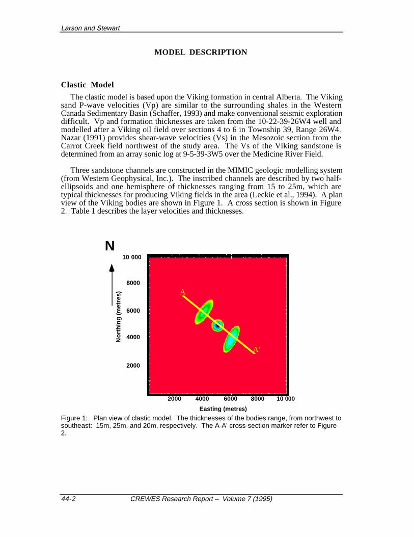
The clastic model is based upon the Viking formation in central Alberta. The Vikingsand P-wave velocities (Vp) are similar to the surrounding shales in the WesternCanada Sedimentary Basin (Schaffer, 1993) and make conventional seismic explorationdifficult. Vp and formation thicknesses are taken from the 10-22-39-26W4 well andmodelled after a Viking oil field over sections 4 to 6 in Township 39, Range 26W4.Nazar (1991) provides shear-wave velocities (Vs) in the Mesozoic section from theCarrot Creek field northwest of the study area. The Vs of the Viking sandstone isdetermined from an array sonic log at 9-5-39-3W5 over the Medicine River Field.

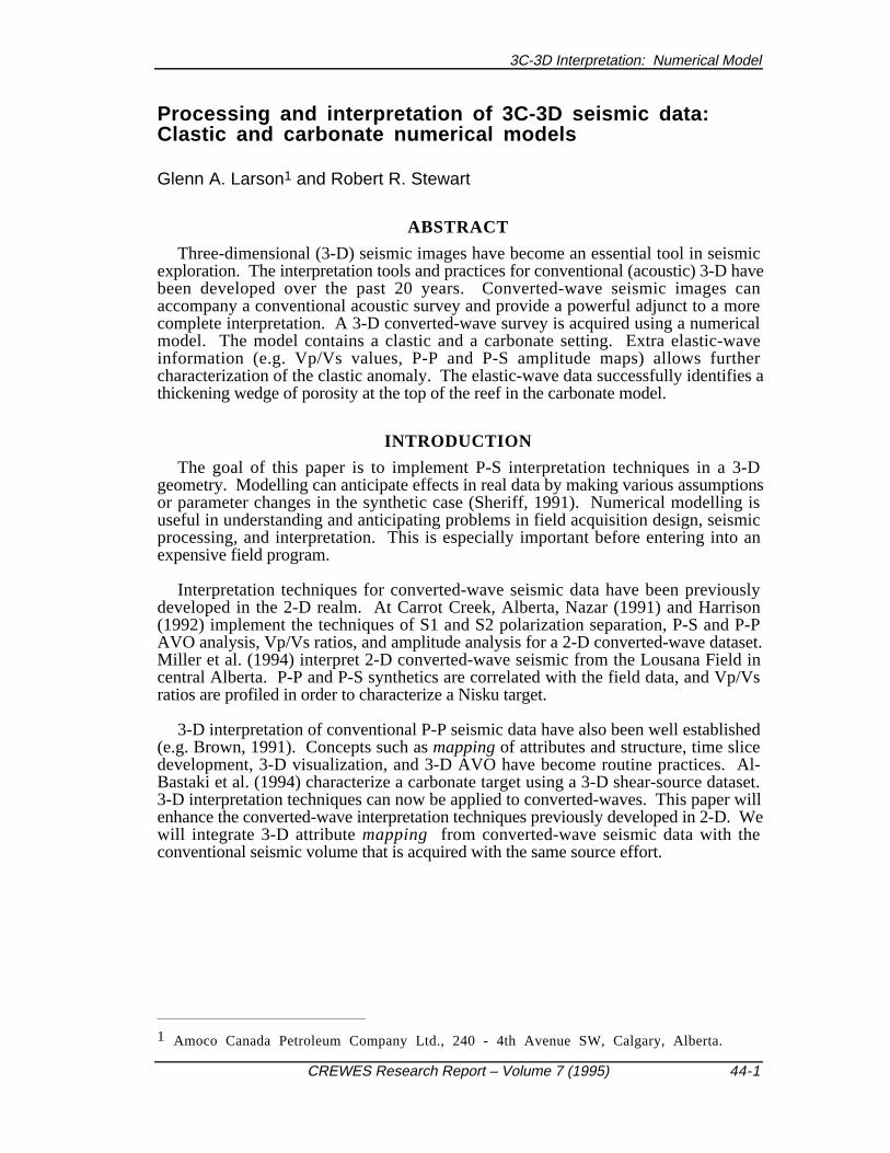
Three sandstone channels are constructed in the MIMIC geologic modelling system(from Western Geophysical, Inc.). The inscribed channels are described by two half-ellipsoids and one hemisphere of thicknesses ranging from 15 to 25m, which aretypical thicknesses for producing Viking fields in the area (Leckie et al., 1994). A planview of the Viking bodies are shown in Figure 1. A cross section is shown in Figure2. Table 1 describes the layer velocities and thicknesses.

Easting (metres)

2000

8000

60004000 10 0008000

2000

6000

4000

10 000N

A

A'

No

rth

ing

(met

res)

Figure 1: Plan view of clastic model. The thicknesses of the bodies range, from northwest tosoutheast: 15m, 25m, and 20m, respectively. The A-A' cross-section marker refer to Figure2.



1 km 800m800m

15m 25m 20m

Surface

1486m

1530m

1370m

1560m

1580m

SecondWhiteSpecksBase ofFish Scales

Joli Fou

Mannville

Viking Shale

TopLayer

Not to Scale

A A'

VikingSand

Figure 2: Cross-section of clastic model.

Layer Depth(m) Vp(m/s) Vs(m/s) Vp/Vs

Top Layer 0 3500 1750 1.87

Second WhiteSpecks (2WS) 1370 3350 1876 1.79

Base of FishScales (BFS) 1486 3280 1574 2.08

Viking Sand 1530 4166 2541 1.64

Viking Shale 1530 4000 2000 2.0

Joli Fou 1560 2771 1330 2.08

Mannville 1580 4100 2457 1.7

Table 1: Clastic model layer velocities and thicknesses

Carbonate model

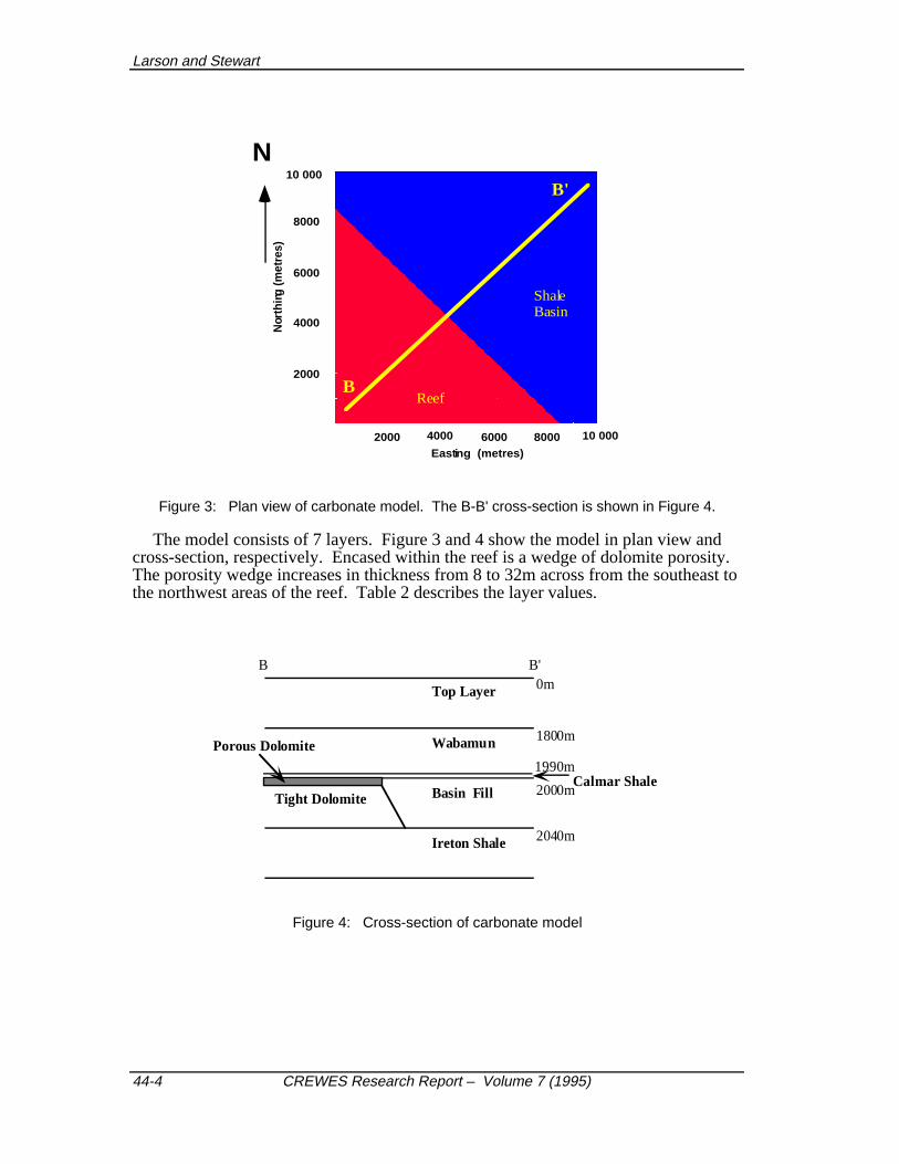
The carbonate model is a stratigraphic trap consisting of a shelf transition fromdolomite to shale. The thicknesses and Vp values for the Wabamun, Nisku, and Iretonare taken from the 10-22-39-26W4 well. The Vs values are calculated from Vp/Vsvalues taken from the Miller et al. (1994) study of the Lousana field southeast of the10-22-39-26W4 location.

Larson and Stewart


Easting (metres)2000

8000

60004000 10 0008000

2000

6000

4000

10 000

N

B

B'

Reef

ShaleBasin

Nor

thin

g (m

etre

s)

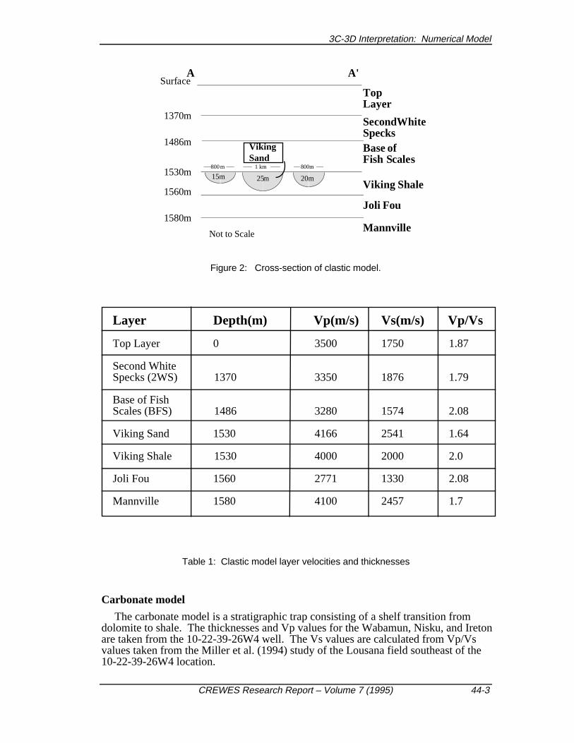
Figure 3: Plan view of carbonate model. The B-B' cross-section is shown in Figure 4.

The model consists of 7 layers. Figure 3 and 4 show the model in plan view andcross-section, respectively. Encased within the reef is a wedge of dolomite porosity.The porosity wedge increases in thickness from 8 to 32m across from the southeast tothe northwest areas of the reef. Table 2 describes the layer values.

Tight Dolomite

Porous Dolomite

Basin FillCalmar Shale

Top Layer

Wabamun

Ireton Shale

0m

1800m

1990m

2000m

2040m

B B'

Figure 4: Cross-section of carbonate model



Layer Depth(m) Vp(m/s) Vs(m/s) Vp/Vs

Top Layer 0 3480 1740 2.0

Wabamun 1800 5995 3177 1.9

Calmar Shale 1990 5400 2592 2.1

Porous Dolomite 2000 5340 3043 1.75

Basin Fill 2000 6400 3200 2.0

Tight Dolomite 2008-2032 7090 3970 1.8

Ireton 2040 5500 2640 2.1

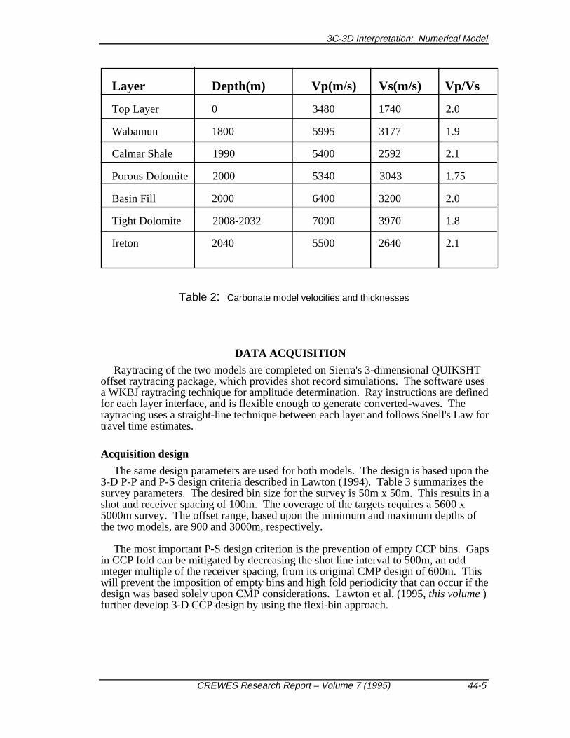
Table 2: Carbonate model velocities and thicknesses

DATA ACQUISITION

Raytracing of the two models are completed on Sierra's 3-dimensional QUIKSHToffset raytracing package, which provides shot record simulations. The software usesa WKBJ raytracing technique for amplitude determination. Ray instructions are definedfor each layer interface, and is flexible enough to generate converted-waves. Theraytracing uses a straight-line technique between each layer and follows Snell's Law fortravel time estimates.

Acquisition design

The same design parameters are used for both models. The design is based upon the3-D P-P and P-S design criteria described in Lawton (1994). Table 3 summarizes thesurvey parameters. The desired bin size for the survey is 50m x 50m. This results in ashot and receiver spacing of 100m. The coverage of the targets requires a 5600 x5000m survey. The offset range, based upon the minimum and maximum depths ofthe two models, are 900 and 3000m, respectively.

The most important P-S design criterion is the prevention of empty CCP bins. Gapsin CCP fold can be mitigated by decreasing the shot line interval to 500m, an oddinteger multiple of the receiver spacing, from its original CMP design of 600m. Thiswill prevent the imposition of empty bins and high fold periodicity that can occur if thedesign was based solely upon CMP considerations. Lawton et al. (1995, this volume )further develop 3-D CCP design by using the flexi-bin approach.

Larson and Stewart


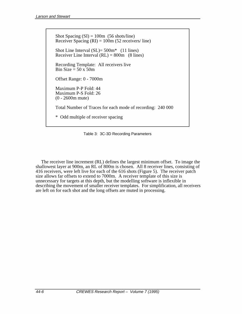
Shot Spacing (SI) = 100m (56 shots/line)Receiver Spacing (RI) = 100m (52 receivers/ line)

Shot Line Interval (SL)= 500m* (11 lines)Receiver Line Interval (RL) = 800m (8 lines)

Recording Template: All receivers liveBin Size = 50 x 50m

Offset Range: 0 - 7000m

Maximum P-P Fold: 44Maximum P-S Fold: 26(0 - 2600m mute)

Total Number of Traces for each mode of recording: 240 000

* Odd multiple of receiver spacing

Table 3: 3C-3D Recording Parameters

The receiver line increment (RL) defines the largest minimum offset. To image theshallowest layer at 900m, an RL of 800m is chosen. All 8 receiver lines, consisting of416 receivers, were left live for each of the 616 shots (Figure 5). The receiver patchsize allows far offsets to extend to 7000m. A receiver template of this size isunnecessary for targets at this depth, but the modelling software is inflexible indescribing the movement of smaller receiver templates. For simplification, all receiversare left on for each shot and the long offsets are muted in processing.



Easting (metres)

2000

8000

60004000 10 0008000

2000

6000

4000

10 000N

No

rth

ing

(met

res)

Receiver Line Axis

Shot

Lin

e A

xis

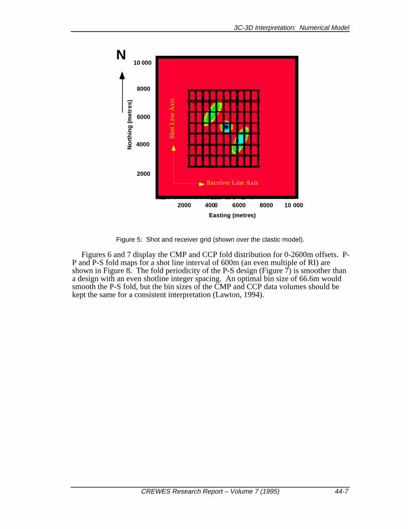
Figure 5: Shot and receiver grid (shown over the clastic model).

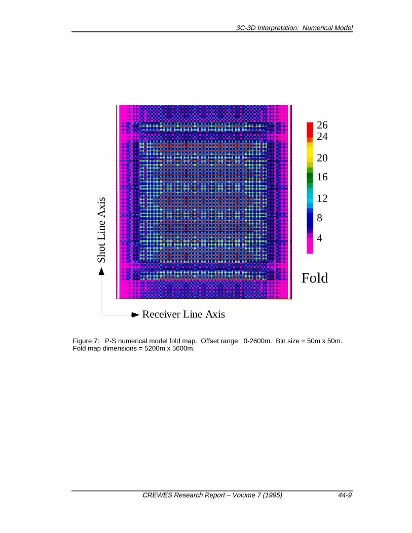
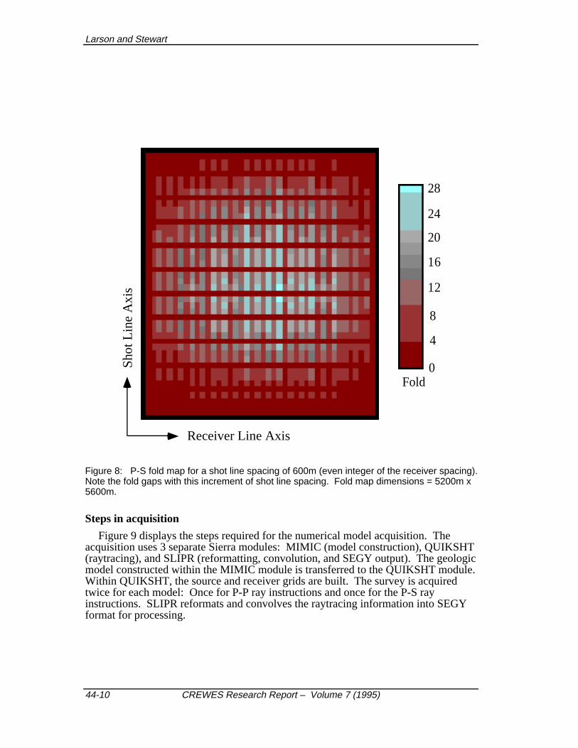
Figures 6 and 7 display the CMP and CCP fold distribution for 0-2600m offsets. P-P and P-S fold maps for a shot line interval of 600m (an even multiple of RI) areshown in Figure 8. The fold periodicity of the P-S design (Figure 7) is smoother thana design with an even shotline integer spacing. An optimal bin size of 66.6m wouldsmooth the P-S fold, but the bin sizes of the CMP and CCP data volumes should bekept the same for a consistent interpretation (Lawton, 1994).

Larson and Stewart


Fold

14

8

10

12

6

4

2

Receiver Line Axis

Shot

Lin

e A

xis

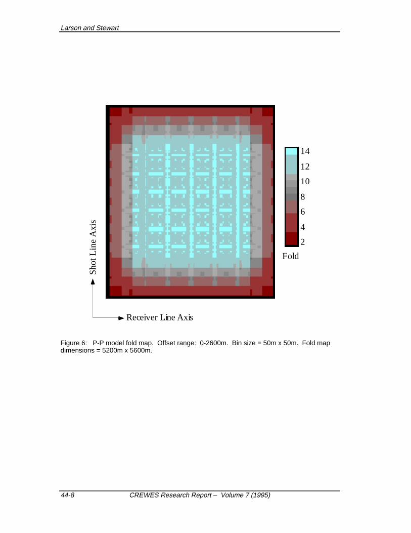
Figure 6: P-P model fold map. Offset range: 0-2600m. Bin size = 50m x 50m. Fold mapdimensions = 5200m x 5600m.



Fold

26

20

4

8

12

24

16

Receiver Line Axis

Shot

Lin

e A

xis

Figure 7: P-S numerical model fold map. Offset range: 0-2600m. Bin size = 50m x 50m.Fold map dimensions = 5200m x 5600m.

Larson and Stewart


0

4

8

12

16

20

24

28

Fold

Receiver Line Axis

Shot

Lin

e A

xis

Figure 8: P-S fold map for a shot line spacing of 600m (even integer of the receiver spacing).Note the fold gaps with this increment of shot line spacing. Fold map dimensions = 5200m x5600m.

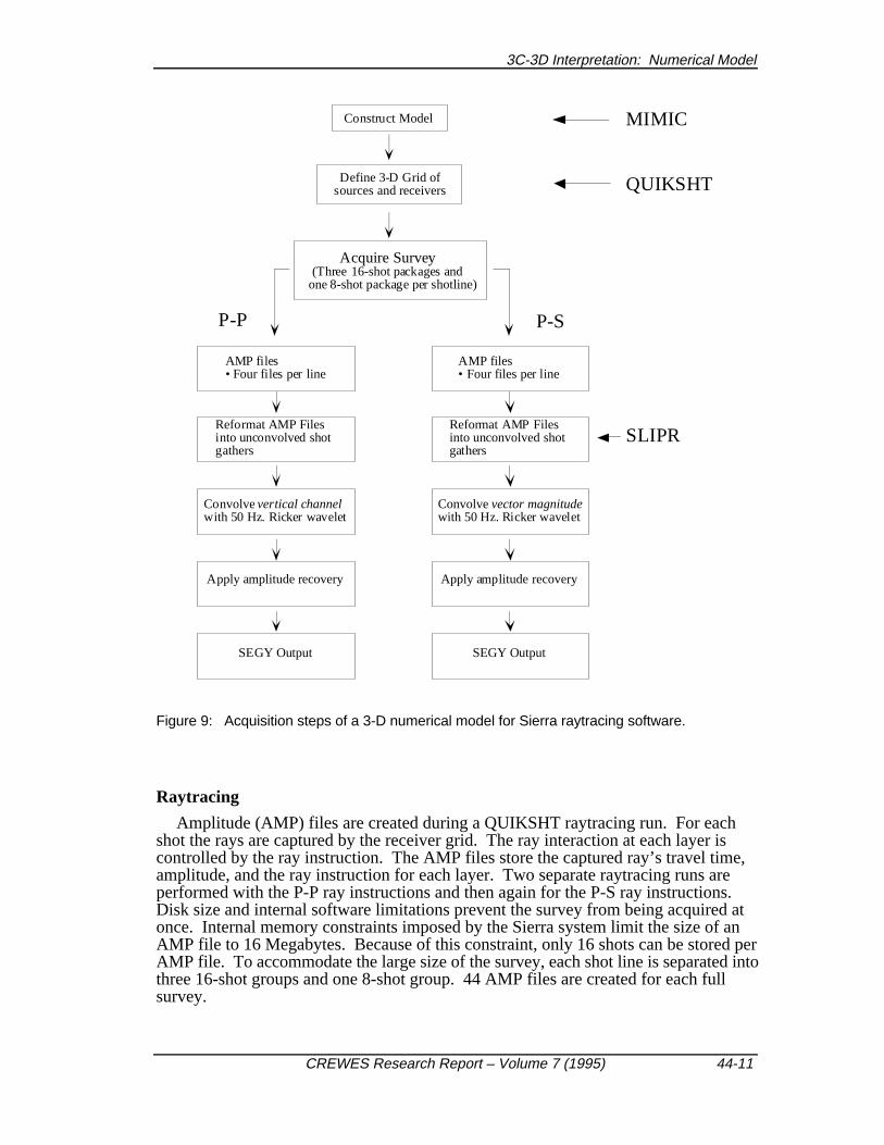
Steps in acquisition

Figure 9 displays the steps required for the numerical model acquisition. Theacquisition uses 3 separate Sierra modules: MIMIC (model construction), QUIKSHT(raytracing), and SLIPR (reformatting, convolution, and SEGY output). The geologicmodel constructed within the MIMIC module is transferred to the QUIKSHT module.Within QUIKSHT, the source and receiver grids are built. The survey is acquiredtwice for each model: Once for P-P ray instructions and once for the P-S rayinstructions. SLIPR reformats and convolves the raytracing information into SEGYformat for processing.



Construct Model

Define 3-D Grid ofsources and receivers

Acquire Survey(Three 16-shot packages and

one 8-shot package per shotline)

AMP files• Four files per line

Reformat AMP Filesinto unconvolved shotgathers

Convolve vertical channelwith 50 Hz. Ricker wavelet

Apply amplitude recovery

SEGY Output

AMP files• Four files per line

Reformat AMP Filesinto unconvolved shotgathers

Convolve vector magnitudewith 50 Hz. Ricker wavelet

Apply amplitude recovery

SEGY Output

MIMIC

QUIKSHT

SLIPR

P-P P-S

Figure 9: Acquisition steps of a 3-D numerical model for Sierra raytracing software.

Raytracing

Amplitude (AMP) files are created during a QUIKSHT raytracing run. For eachshot the rays are captured by the receiver grid. The ray interaction at each layer iscontrolled by the ray instruction. The AMP files store the captured ray’s travel time,amplitude, and the ray instruction for each layer. Two separate raytracing runs areperformed with the P-P ray instructions and then again for the P-S ray instructions.Disk size and internal software limitations prevent the survey from being acquired atonce. Internal memory constraints imposed by the Sierra system limit the size of anAMP file to 16 Megabytes. Because of this constraint, only 16 shots can be stored perAMP file. To accommodate the large size of the survey, each shot line is separated intothree 16-shot groups and one 8-shot group. 44 AMP files are created for each fullsurvey.

Larson and Stewart


Reformatting and convolution

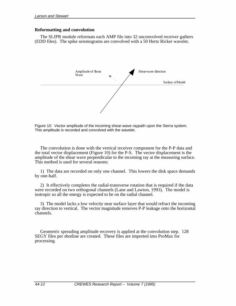
The SLIPR module reformats each AMP file into 32 unconvolved receiver gathers(EDD files). The spike seismograms are convolved with a 50 Hertz Ricker wavelet.

Shear-wave directionAmplitude of ShearWave

Surface of Model

Figure 10: Vector amplitude of the incoming shear-wave raypath upon the Sierra system.This amplitude is recorded and convolved with the wavelet.

The convolution is done with the vertical receiver component for the P-P data andthe total vector displacement (Figure 10) for the P-S. The vector displacement is theamplitude of the shear wave perpendicular to the incoming ray at the measuring surface.This method is used for several reasons:

1) The data are recorded on only one channel. This lowers the disk space demandsby one-half.

2) It effectively completes the radial-transverse rotation that is required if the datawere recorded on two orthogonal channels (Lane and Lawton, 1993). The model isisotropic so all the energy is expected to be on the radial channel.

3) The model lacks a low velocity near surface layer that would refract the incomingray direction to vertical. The vector magnitude removes P-P leakage onto the horizontalchannels.

Geometric spreading amplitude recovery is applied at the convolution step. 128SEGY files per shotline are created. These files are imported into ProMax forprocessing.



PROCESSING

Pre-processing

Prior to geometry assignment, the individual shot line SEGY files are combined intoa full 3-D survey. The final Sierra output presents 1408 separate SEGY files each forthe P-P and P-S surveys. Each file consists of 16 or 8 shot gathers sorted for eachreceiver line. To create one large file suitable for 3-D processing the following stepsare taken:

1) The SEGY files are input by shot line. For each shot line, the FFID (field fileidentification number) header words are renumbered sequentially.

2) The shotlines are sorted by FFID and channel number. Each new shotlineensemble is written and merged together to form 56 shot gathers consisting of 416receivers.

3) Repeat steps 1 and 2 for the remaining shot lines.

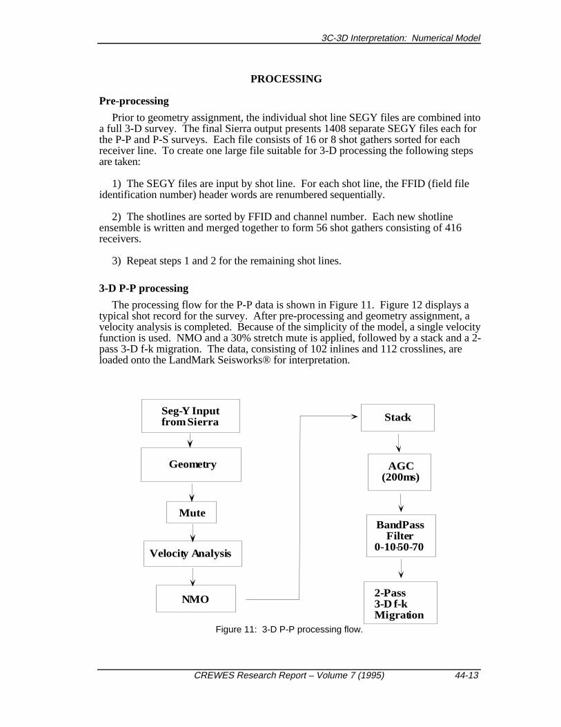
3-D P-P processing

The processing flow for the P-P data is shown in Figure 11. Figure 12 displays atypical shot record for the survey. After pre-processing and geometry assignment, avelocity analysis is completed. Because of the simplicity of the model, a single velocityfunction is used. NMO and a 30% stretch mute is applied, followed by a stack and a 2-pass 3-D f-k migration. The data, consisting of 102 inlines and 112 crosslines, areloaded onto the LandMark Seisworks® for interpretation.

Mute

Velocity Analysis

NMO

Stack

Geometry

Seg-Y Inputfrom Sierra

2-Pass3-D f-kMigration

AGC(200ms)

BandPassFilter

0-10-50-70

Figure 11: 3-D P-P processing flow.

Larson and Stewart


700

800

900

1000

1200

1300

Receiver Line 2 Receiver Line 3 Receiver Line 4

Tim

e (m

s)

2WS

Viking

Mannville

1400

1500

1100

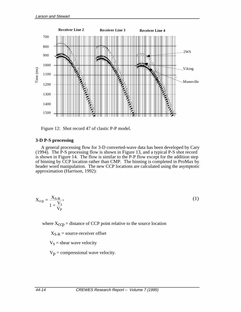
Figure 12: Shot record 47 of clastic P-P model.

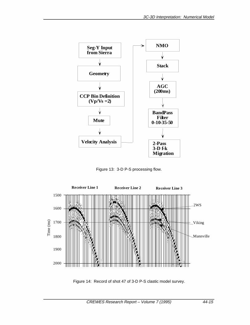
3-D P-S processing

A general processing flow for 3-D converted-wave data has been developed by Cary(1994). The P-S processing flow is shown in Figure 13, and a typical P-S shot recordis shown in Figure 14. The flow is similar to the P-P flow except for the addition stepof binning by CCP location rather than CMP. The binning is completed in ProMax byheader word manipulation. The new CCP locations are calculated using the asymptoticapproximation (Harrison, 1992):

Xccp = XS-R

1 + VsVP

, (1)

where Xccp = distance of CCP point relative to the source location

XS-R = source-receiver offset

Vs = shear wave velocity

Vp = compressional wave velocity.



Geometry

CCP Bin Definition(Vp/Vs =2)

Seg-Y Inputfrom Sierra

Mute

Velocity Analysis

NMO

Stack

2-Pass3-D f-kMigration

AGC(200ms)

BandPassFilter

0-10-35-50

Figure 13: 3-D P-S processing flow.

1500

1600

1700

1800

1900

2000

Receiver Line 1 Receiver Line 2 Receiver Line 3

Tim

e (m

s)

2WS

Viking

Mannville

Figure 14: Record of shot 47 of 3-D P-S clastic model survey.

Larson and Stewart


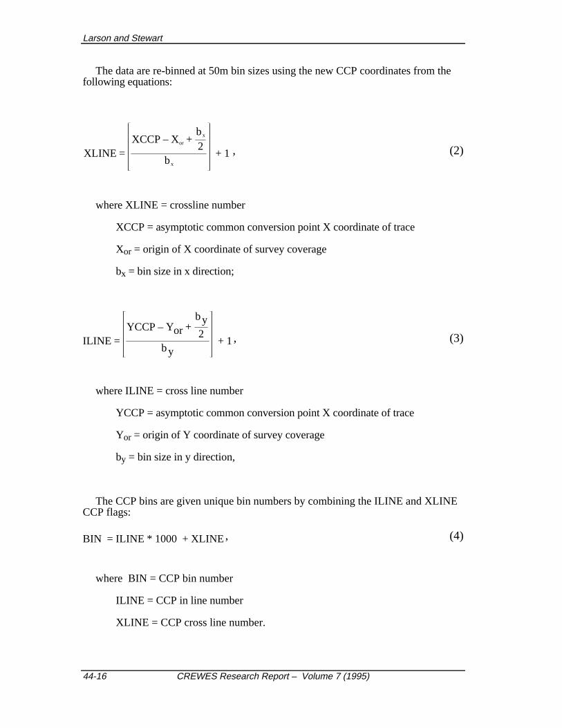
The data are re-binned at 50m bin sizes using the new CCP coordinates from thefollowing equations:

XLINE =XCCP – Xor +

bx

2bx

+ 1 , (2)

where XLINE = crossline number

XCCP = asymptotic common conversion point X coordinate of trace

Xor = origin of X coordinate of survey coverage

bx = bin size in x direction;

ILINE =YCCP – Yor +

by2

by+ 1 , (3)

where ILINE = cross line number

YCCP = asymptotic common conversion point X coordinate of trace

Yor = origin of Y coordinate of survey coverage

by = bin size in y direction,

The CCP bins are given unique bin numbers by combining the ILINE and XLINECCP flags:

BIN = ILINE * 1000 + XLINE , (4)

where BIN = CCP bin number

ILINE = CCP in line number

XLINE = CCP cross line number.



The trace header values of CDP_X, CDP_Y, and the CDP bin numbers are replacedwith the corresponding CCP values. With this replacement, converted-wave velocityanalysis, stacking, and migration are completed with the standard CMP processeswithin ProMax.

The NMO correction does not incorporate the improved P-S NMO correction ofSlotboom (1992) because of the high offset-to-depth ratio and because the correctionhas yet to be implemented in the ProMax processing system. A 10-20-35-50 Ormsbyzero phase bandpass filter is applied to the P-S data. The filter lowers the bandwidthwith respect to the P-P volume (0-10-50-60 Ormsby filter) to anticipate a lower fieldresponse for shear data. For the deeper carbonate model, the P-S volume is filteredsomewhat lower with a 0-20-35-40 Ormsby bandpass filter. This is done to anticipatea reduction in frequency bandwidth at greater depth (Miller et al, 1994). The P-S stackis migrated with 95% of the RMS velocities from the velocity analysis (Harrison andStewart, 1993). The migration is a 2-pass 3-D f-k method.

INTERPRETATION

Clastic model interpretation

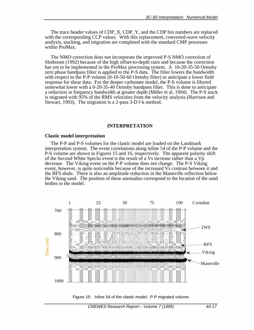
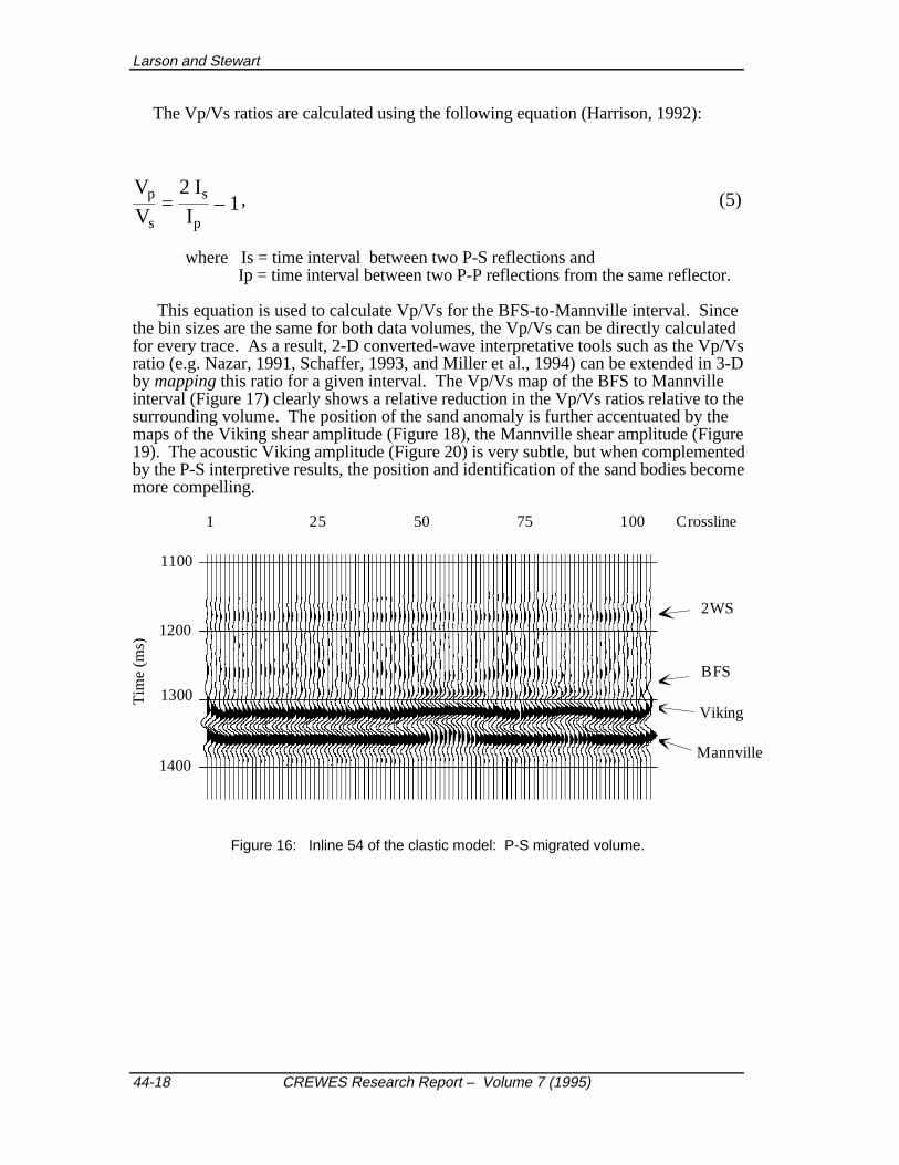
The P-P and P-S volumes for the clastic model are loaded on the Landmarkinterpretation system. The event correlations along inline 54 of the P-P volume and theP-S volume are shown in Figures 15 and 16, respectively. The apparent polarity shiftof the Second White Specks event is the result of a Vs increase rather than a Vpdecrease. The Viking event on the P-P volume does not change. The P-S Vikingevent, however, is quite noticeable because of the increased Vs contrast between it andthe BFS shale. There is also an amplitude reduction in the Mannville reflection belowthe Viking sand. The position of these anomalies correspond to the location of the sandbodies in the model.

700

800

900

1000

1 25 75 100 Crossline50

Mannville

Viking

BFS

2WS

Tim

e (m

s)

Figure 15: Inline 54 of the clastic model: P-P migrated volume.

Larson and Stewart


The Vp/Vs ratios are calculated using the following equation (Harrison, 1992):

Vp

Vs=

2 Is

Ip– 1 , (5)

where Is = time interval between two P-S reflections andIp = time interval between two P-P reflections from the same reflector.

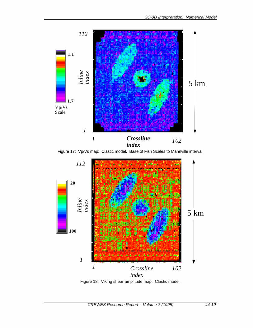
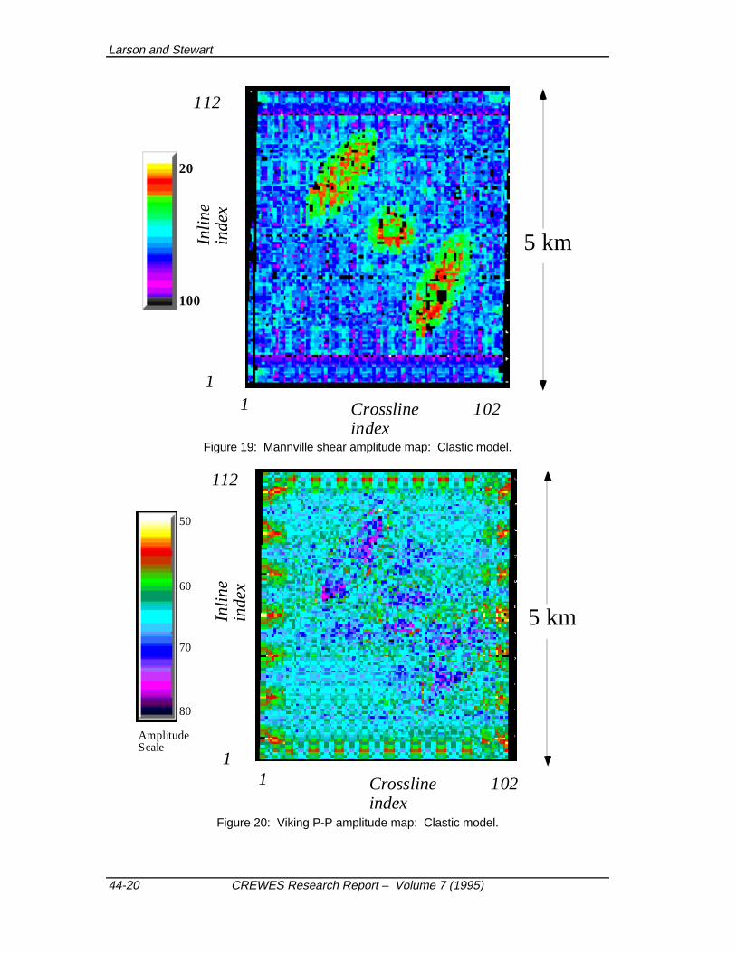
This equation is used to calculate Vp/Vs for the BFS-to-Mannville interval. Sincethe bin sizes are the same for both data volumes, the Vp/Vs can be directly calculatedfor every trace. As a result, 2-D converted-wave interpretative tools such as the Vp/Vsratio (e.g. Nazar, 1991, Schaffer, 1993, and Miller et al., 1994) can be extended in 3-Dby mapping this ratio for a given interval. The Vp/Vs map of the BFS to Mannvilleinterval (Figure 17) clearly shows a relative reduction in the Vp/Vs ratios relative to thesurrounding volume. The position of the sand anomaly is further accentuated by themaps of the Viking shear amplitude (Figure 18), the Mannville shear amplitude (Figure19). The acoustic Viking amplitude (Figure 20) is very subtle, but when complementedby the P-S interpretive results, the position and identification of the sand bodies becomemore compelling.

1 75 100 Crossline50

Mannville

Viking

BFS

2WS

1100

1200

1300

1400

Tim

e (m

s)

25

Figure 16: Inline 54 of the clastic model: P-S migrated volume.



1.1

1.7Vp/VsScale

5 km

Crosslineindex

1 102

1

112

Inli

nein

dex

Figure 17: Vp/Vs map: Clastic model. Base of Fish Scales to Mannville interval.

5 km

20

100

Crosslineindex

1 102

1

112

Inli

nein

dex

Figure 18: Viking shear amplitude map: Clastic model.

Larson and Stewart


5 km

20

100

Crosslineindex

1 102

1

112

Inli

nein

dex

Figure 19: Mannville shear amplitude map: Clastic model.

5 km

Crosslineindex

1 102

1

112

Inli

nein

dex

50

80

60

70

AmplitudeScale

Figure 20: Viking P-P amplitude map: Clastic model.



From this example, the value of S-waves in imaging the clastic model is high. Theexclusive use of acoustic seismic data would not be capable of unambiguously imagingthe sand bodies. Detection of small changes in Vp/Vs in a map view with the power of3-D pattern recognition can reveal subtler features than a 2-D profile can. The inclusionof shear data volumes for this isotropic model has doubled the amount of interpretabledata and has enhanced the interpretation. It has also added confidence to theinterpretation.

Carbonate model interpretation

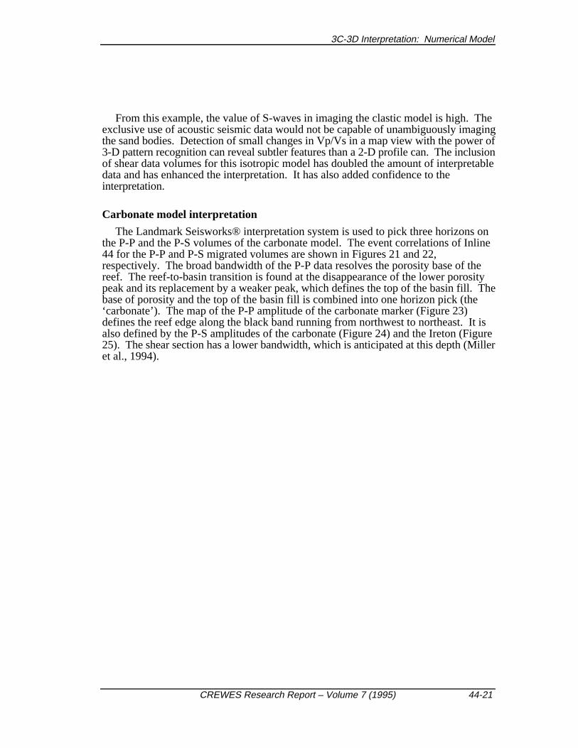
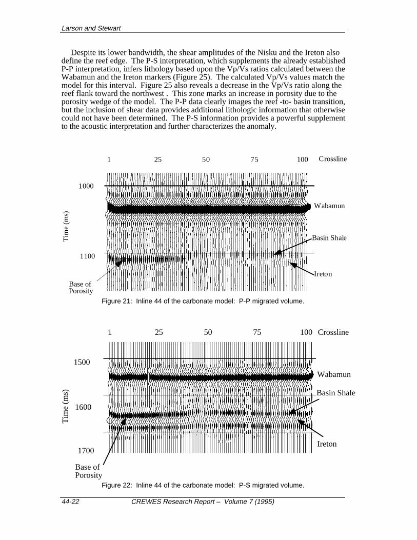
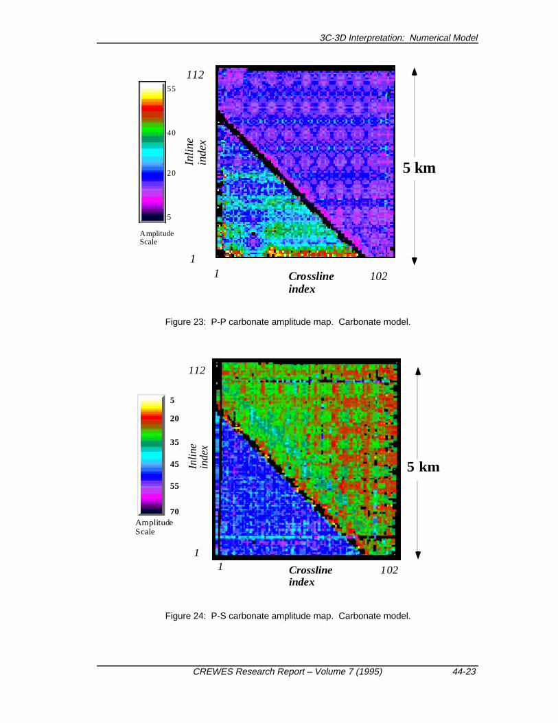
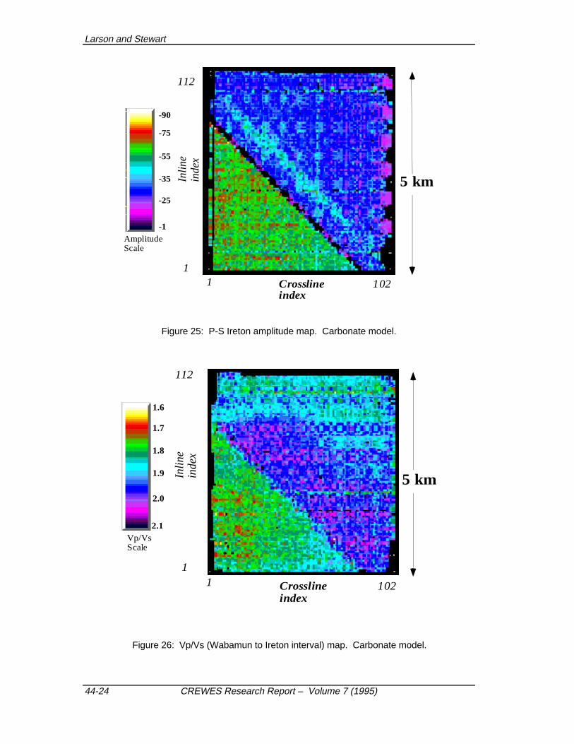
The Landmark Seisworks® interpretation system is used to pick three horizons onthe P-P and the P-S volumes of the carbonate model. The event correlations of Inline44 for the P-P and P-S migrated volumes are shown in Figures 21 and 22,respectively. The broad bandwidth of the P-P data resolves the porosity base of thereef. The reef-to-basin transition is found at the disappearance of the lower porositypeak and its replacement by a weaker peak, which defines the top of the basin fill. Thebase of porosity and the top of the basin fill is combined into one horizon pick (the‘carbonate’). The map of the P-P amplitude of the carbonate marker (Figure 23)defines the reef edge along the black band running from northwest to northeast. It isalso defined by the P-S amplitudes of the carbonate (Figure 24) and the Ireton (Figure25). The shear section has a lower bandwidth, which is anticipated at this depth (Milleret al., 1994).

Larson and Stewart


Despite its lower bandwidth, the shear amplitudes of the Nisku and the Ireton alsodefine the reef edge. The P-S interpretation, which supplements the already establishedP-P interpretation, infers lithology based upon the Vp/Vs ratios calculated between theWabamun and the Ireton markers (Figure 25). The calculated Vp/Vs values match themodel for this interval. Figure 25 also reveals a decrease in the Vp/Vs ratio along thereef flank toward the northwest . This zone marks an increase in porosity due to theporosity wedge of the model. The P-P data clearly images the reef -to- basin transition,but the inclusion of shear data provides additional lithologic information that otherwisecould not have been determined. The P-S information provides a powerful supplementto the acoustic interpretation and further characterizes the anomaly.

1000

1100

Tim

e (m

s)


Ireton

Basin Shale

Wabamun

Base ofPorosity

25

Figure 21: Inline 44 of the carbonate model: P-P migrated volume.

1500

1600

1700


Ireton

Basin Shale

Wabamun

Tim

e (m

s)

Base ofPorosity

25

Figure 22: Inline 44 of the carbonate model: P-S migrated volume.



5 km

Crosslineindex

1 102

1

112

Inli

nein

dex

55

5

40

20

AmplitudeScale

Figure 23: P-P carbonate amplitude map. Carbonate model.

5

70AmplitudeScale

5 km

Crosslineindex

1 102

1

112

Inlin

ein

dex35

55

20

45

Figure 24: P-S carbonate amplitude map. Carbonate model.

Larson and Stewart


-90

-1AmplitudeScale

5 km

Crosslineindex

1 102

1

112

Inlin

ein

dex-55

-25

-75

-35

Figure 25: P-S Ireton amplitude map. Carbonate model.

1.6

2.1Vp/VsScale

5 km

Crosslineindex

1 102

1

112

Inlin

ein

dex1.8

2.0

1.7

1.9

Figure 26: Vp/Vs (Wabamun to Ireton interval) map. Carbonate model.



TUNING EFFECTS UPON VP/VS RATIO CALCULATIONS

The Vp/Vs values for the BFS-to-Mannville interval of the clastic model are lowerthan the modelled values. Wavelet tuning effects may be partially responsible for thisunderestimation. The Vp/Vs calculations are based upon the interpreted time structuresof the BFS and Mannville, and they may be affected by wavelet tuning within the JoliFou shale.

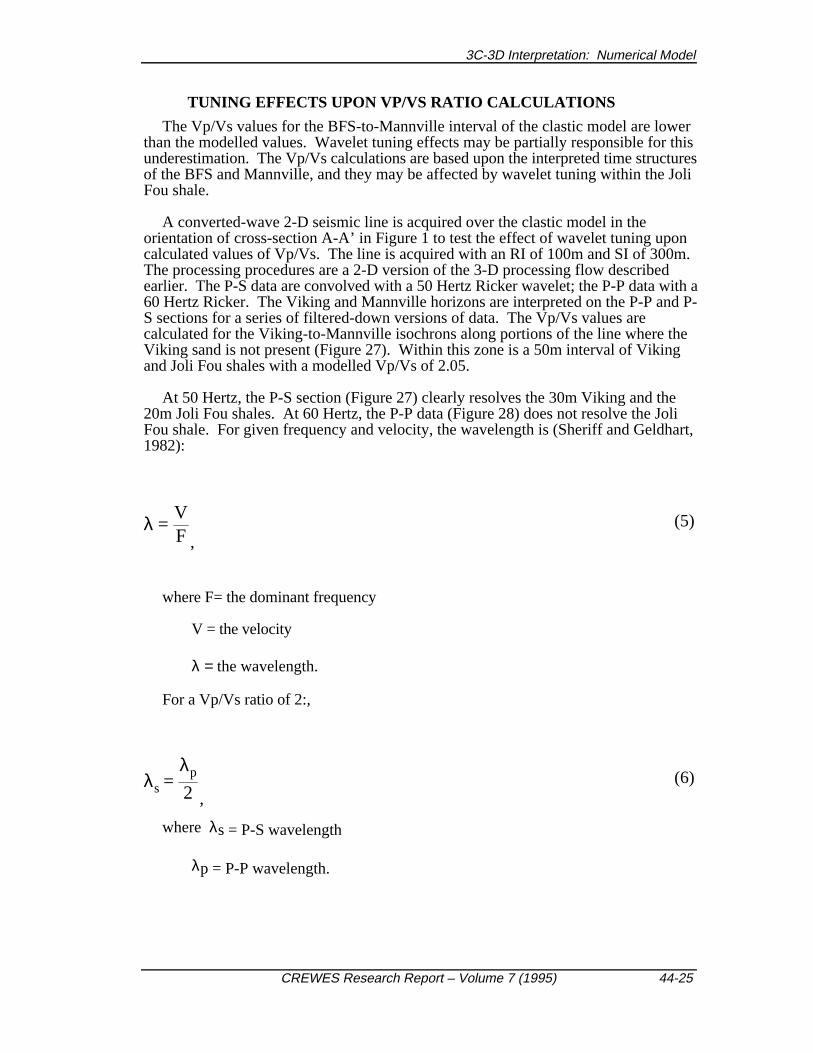
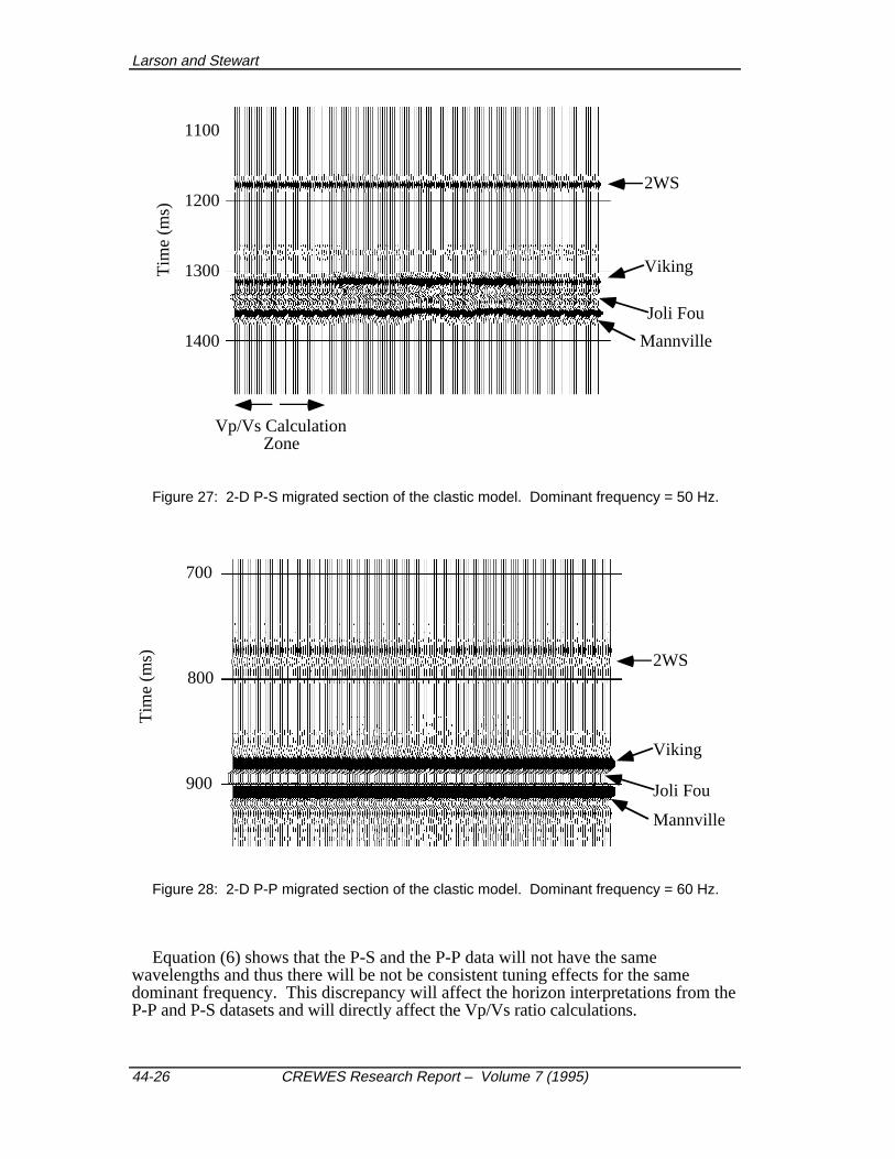
A converted-wave 2-D seismic line is acquired over the clastic model in theorientation of cross-section A-A’ in Figure 1 to test the effect of wavelet tuning uponcalculated values of Vp/Vs. The line is acquired with an RI of 100m and SI of 300m.The processing procedures are a 2-D version of the 3-D processing flow describedearlier. The P-S data are convolved with a 50 Hertz Ricker wavelet; the P-P data with a60 Hertz Ricker. The Viking and Mannville horizons are interpreted on the P-P and P-S sections for a series of filtered-down versions of data. The Vp/Vs values arecalculated for the Viking-to-Mannville isochrons along portions of the line where theViking sand is not present (Figure 27). Within this zone is a 50m interval of Vikingand Joli Fou shales with a modelled Vp/Vs of 2.05.

At 50 Hertz, the P-S section (Figure 27) clearly resolves the 30m Viking and the20m Joli Fou shales. At 60 Hertz, the P-P data (Figure 28) does not resolve the JoliFou shale. For given frequency and velocity, the wavelength is (Sheriff and Geldhart,1982):

λ =

VF ,

(5)

where F= the dominant frequency

V = the velocity

λ = the wavelength.

For a Vp/Vs ratio of 2:,

λs =

λp

2 ,(6)

where λs = P-S wavelength

λp = P-P wavelength.

Larson and Stewart


Vp/Vs CalculationZone

1100

1200

1300Tim

e (m

s)

Viking

Mannville

2WS

Joli Fou

1400

Figure 27: 2-D P-S migrated section of the clastic model. Dominant frequency = 50 Hz.

700

800

900

Tim

e (m

s)

Viking

Mannville

2WS

Joli Fou

Figure 28: 2-D P-P migrated section of the clastic model. Dominant frequency = 60 Hz.

Equation (6) shows that the P-S and the P-P data will not have the samewavelengths and thus there will be not be consistent tuning effects for the samedominant frequency. This discrepancy will affect the horizon interpretations from theP-P and P-S datasets and will directly affect the Vp/Vs ratio calculations.



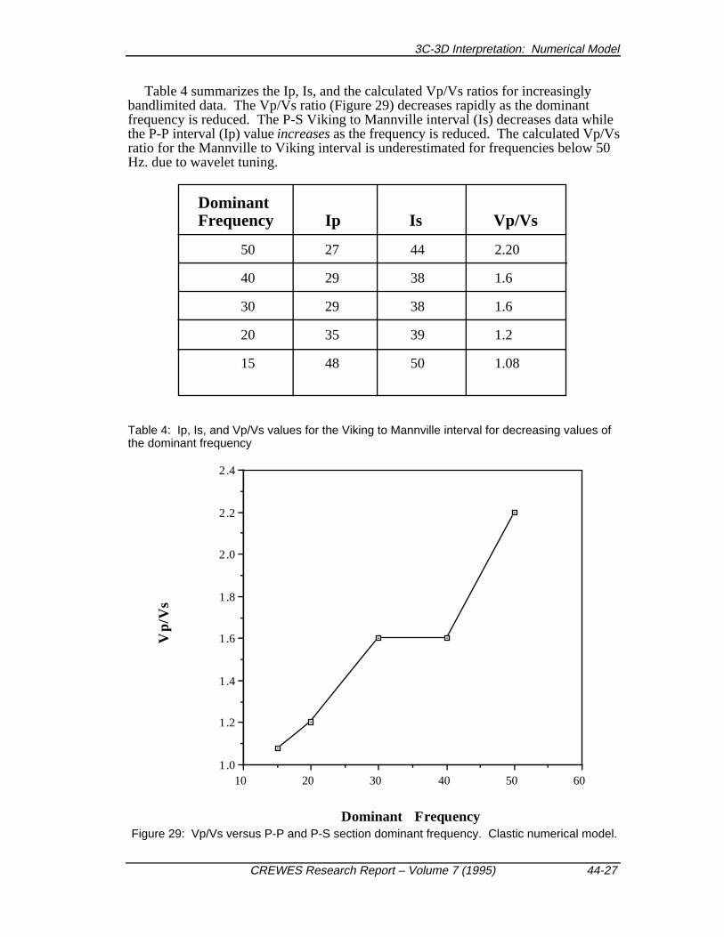
Table 4 summarizes the Ip, Is, and the calculated Vp/Vs ratios for increasinglybandlimited data. The Vp/Vs ratio (Figure 29) decreases rapidly as the dominantfrequency is reduced. The P-S Viking to Mannville interval (Is) decreases data whilethe P-P interval (Ip) value increases as the frequency is reduced. The calculated Vp/Vsratio for the Mannville to Viking interval is underestimated for frequencies below 50Hz. due to wavelet tuning.

DominantFrequency Ip Is Vp/Vs

50 27 44 2.20

40 29 38 1.6

30 29 38 1.6

20 35 39 1.2

15 48 50 1.08

Table 4: Ip, Is, and Vp/Vs values for the Viking to Mannville interval for decreasing values ofthe dominant frequency

6050403020101.0

1.2

1.4

1.6

1.8

2.0

2.2

2.4

Dominant Frequency

Vp

/Vs

Figure 29: Vp/Vs versus P-P and P-S section dominant frequency. Clastic numerical model.

Larson and Stewart


DominantFrequency Ip Is Vp/Vs

50 29 44 2.03

40 29 38 1.6

30 29 38 1.6

20 29 39 1.7

15 29 50 2.4

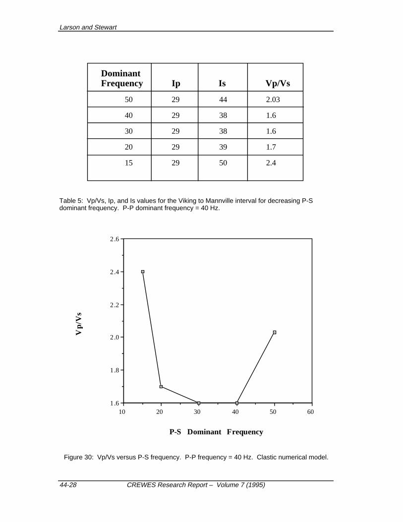
Table 5: Vp/Vs, Ip, and Is values for the Viking to Mannville interval for decreasing P-Sdominant frequency. P-P dominant frequency = 40 Hz.

6050403020101.6

1.8

2.0

2.2

2.4

2.6

P-S Dominant Frequency

Vp

/Vs

Figure 30: Vp/Vs versus P-S frequency. P-P frequency = 40 Hz. Clastic numerical model.



Figure 30 displays the calculated Vp/Vs versus the dominant frequency of the P-Swavelet for a constant P-P frequency of 40 Hz. As the P-S frequency decreases, theVp/Vs ratio is underestimated by 20% in the 20 to 40 Hertz range, but is overestimatedfor very low frequencies. Tatham and McCormack (1989) recommend narrowintervals to calculate Vp/Vs ratios, but for low frequencies, these calculations may becompromised by tuning. Wavelet effects in Vp/Vs ratio calculations have been notedby Miller et al. (1994). Wavelet tuning has a serious effect upon the absolute value ofthe Vp/Vs ratio, but the relative changes of Vp/Vs should remain intact, if the wavelet isconsistent throughout both datasets.

CONCLUSIONS

The two isotropic models show that the use of 3-D P-S data provides supplementaryinformation to the acoustic 3-D survey. In the sand model, the shear is indispensable indelineating the Viking sands. In the reef model, the P-P data can adequately image thereef-to-basin transition. Comparative time intervals between the P-P and the P-S dataresult in Vp/Vs maps that can provide lithologic and thickness indicators. Combiningthis information in a 3-D measurement with the acoustic survey provides a moredetailed interpretation; one which could not be achieved with acoustic data exclusively.

Differences in wavelet tuning between the P-P and the P-S wavelets may alter theabsolute value of the Vp/Vs ratio maps. The relative difference, however, shouldremain intact and allow consistent mapping.

ACKNOWLEDGMENTS

Landmark Graphics Corporation generously donated their Seisworks3Dinterpretation software and the ProMax3D processing system. Western Geophysical,Inc. is thanked for its MIMIC modelling system donation. Shaowu Wang provideduseful processing discussion and assistance. Sue Miller gave insightful suggestions onconverted-wave interpretation.

REFERENCES

Al-Bastaki, A.R., Arestad, J.F., Bard, K., Mattocks, B., Rolla, M.R., Sarmiento, V., Windells, R.,1994, Progress report on the characterization of Nisku carbonate reservoirs: Joffre field, south-central Alberta, Canada, in: Reservoir characterization project - phase 5 report, ColoradoSchool of Mines.

Brown, A.R., 1991, Interpretation of three-dimensional seismic data: AAPG Memoir 42, AmericanAssociation of Petroleum Geologists.

Cary, P.W., 1994, 3-D converted-wave seismic processing: CREWES Research Report, 6, 31-1 - 31-10.

Harrison, M.P., 1992, Processing of P-SV surface-seismic data: anisotropy analysis, dip moveout, andmigration: PhD. dissertation, The University of Calgary.

Harrison, M., and Stewart, R.R., 1993, Poststack migration of P-SV seismic data: Geophysics, 58,1127-1135.

Lawton, D.C., 1994, Acquisition design of 3-D converted-waves: CREWES Research Report, 6, 23-1- 23-23.

Lawton, D.C., Stewart, R.R., Cordsen, A., and Hrycak, S., Advances in 3C-3D design for converted-waves: CREWES Research Report, 7, this volume.

Larson and Stewart


Leckie, D.A., Bhattacharya, J.P., Bloch, J., Gilboy, C.F., Norris, B, 1994. CretaceousColorado/Alberta group. In: Geological Atlas of the Western Canada Sedimentary Basin.G.D. Mossop and I. Shetson (comps.). Calgary, Canadian Society of Petroleum Geologistsand Alberta Research Council, chpt. 20.

Miller, S.L.M, Harrison, M.P., Lawton, D.C., Stewart, R.R., and Szata, K.J., 1994, Analysis of P-Pand P-SV seismic data from Lousana, Alberta: CREWES Research Report, 6, 7-1 - 7-24.

Nazar, B.D., 1991, An interpretive study of multicomponent seismic data from the Carrot Creek area ofwest-central Alberta: M.Sc. thesis, The University of Calgary.

Schaffer, A., 1993, Binning, static correction, and interpretation of P-SV surface-seismic data: M.Sc.thesis, The University of Calgary.

Sherrif, R.E., 1991, Dictionary of geophysical terms, SEG.Sheriff, R.E., and Geldart, L.P., 1982, Exploration Seismology, vol.1. Cambridge University Press.Slotboom, R.T., 1990, Converted-wave (P-SV) moveout estimation: 60th Ann. Internat. Mtg. Soc.

Expl. Geophys., Expanded Abstracts, 1104-1106.Tatham, R.H. and McCormack, M.D., 1991, Multicomponent seismology in petroleum exploration:

Investigations in geophysics - 6, Society of Exploration Geophysicists.

Date post:	21-May-2018
Category:	Documents
Upload:	trankien
View:	217 times
Download:	0 times

Processing and interpretation of 3C-3D seismic data ... · Three-dimensional (3-D) seismic images...

Documents