198
Didier Faivre

Didier Faivre
2
Digital rate options and applications to exotic swapsComplex Products : digital, steepner, ratchet…Bermuda swaptionsCallablesAppendixes :Standard Deviations vs VolatilitiesSABRCorrelation issuesLGMRisk-Management of exotics
3
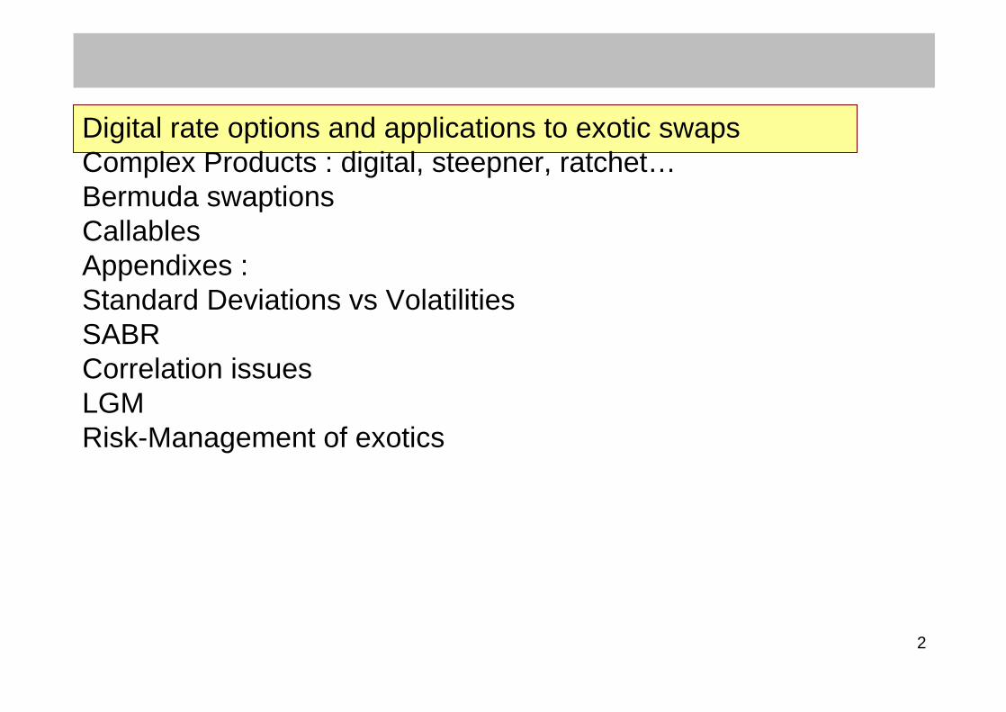
Digital options: the payoff is binary, nil or fixed, in view of a barrier on an underlying security
Example : digital on 3-month Euribor/ Strike (K)
MechanismAt maturity of each 3 month period:
If Euribor < K the buyer receives 0If Euribor > K The buyer receives : Notional × « Pay out » ×NJE/360
Profit/Loss chart:
Euribor
Profit
KPay out
Premium
Digital rate options

4
Profit/Loss chart:
S
Premium
Profit
Euribor
Pay out
Digital rate options

5
example: sell a digital option with payoff equal to 2 % if the 3-month interest rate is higher than 4 %
possible hedging modality: buy a call at 3 % and sell a call at 5 % with same initial nominal amount of the digital option (the approximation of a digital option by using a call spread).
Digital rate options

6
3-month rate
Intrinsic value
barrier
0 5 %
premium
3 % 4 %
digital Call spread
Digital rate options

7
The barrier is suitably replicated by reducing the spread of 200to 20 bp (buying a call at 3.9% and selling a call at 4.10% for the bank selling the digital).
The equalisation of the payoff therefore implies multiplying thenominal amount by 10.
A digital option therefore corresponds to a leverage effect on an options spread.
Digital rate options
8
Digital rate options
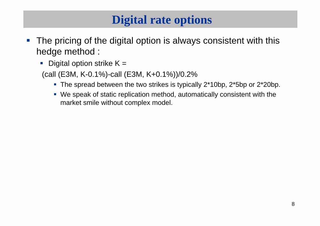
The pricing of the digital option is always consistent with thishedge method :
Digital option strike K =(call (E3M, K-0.1%)-call (E3M, K+0.1%))/0.2%
The spread between the two strikes is typically 2*10bp, 2*5bp or 2*20bp.We speak of static replication method, automatically consistent with the market smile without complex model.
9
Digital rate options
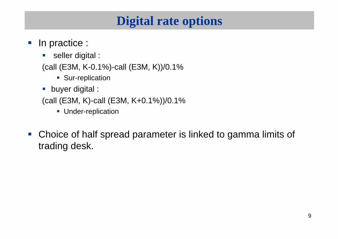
In practice :seller digital :
(call (E3M, K-0.1%)-call (E3M, K))/0.1%Sur-replication
buyer digital : (call (E3M, K)-call (E3M, K+0.1%))/0.1%
Under-replication
Choice of half spread parameter is linked to gamma limits of trading desk.

10
Digital rate options
3-month rate
Intrinsic value
0
KK-0.1 %
1+premium
1%1.0
3 KME
K+0.1 %
1%1.0
3 KME
Sur-replicationUnder-replication
premium

11
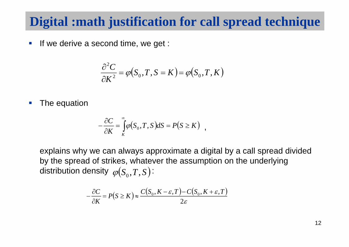
Digital :math justification for call spread technique
Let have and underlying with initial value and density
The price of a call (with premium paid at maturity T) is :
Then
0S
dSSTSKSTKSCK
,,,, 00
STS ,,0
KK
KK
dSSTSdSSTSKSTSKKSTSK
dSSTSKdSSTSSKK
C
,,,,,,,,
,,,,
0000
00
12
Digital :math justification for call spread technique
If we derive a second time, we get :
The equation
,
explains why we can always approximate a digital by a call spread dividedby the spread of strikes, whatever the assumption on the underlyingdistribution density :
KTSKSTSK
C,,,, 002
2
KSPdSSTSK
C
K
,,0
STS ,,0
2
,,,, 00 TKSCTKSCKSP
K
C

13
Digital :math justification for call spread technique
Indeed, it’s important to see the previous demonstration is general and doesn’t rely on any assumption on .
If we now use the (Lognormal) B&S framework, we get :
In pratice, prices of digital using the call-spread method or the analyticalB&S formula (lognormal or normal), leads to very different prices.
2dNKSPK
C

14
Digital rate options
Other pay-off :Let’s note :
bpKK
bpKK
bpKK
bpKK
KK
uprightup
upleftup
downrightdown
downleftdown
updown
10
10
10
10
15
Digital rate options
We have the following replication formulas :
leftup
rightup
rightup
leftup
up
leftdown
rightdown
rightdown
leftdown
down
KK
K,MECallK,MECallKMEdigitloor"digital "f
KK
K,MECallK,MECallKMEdigitap"digital "c
3313)2
333 )1
leftup
rightup
rightup
leftup
leftdown
rightdown
rightdown
leftdown
updown
leftup
rightup
rightup
leftup
leftdown
rightdown
rightdown
leftdown
updown
KK
KMECallKMECall
KK
KMECallKMECall
KKMEdigitt"digital"ou
KK
KMECallKMECall
KK
KMECallKMECall
KKMEdigitn"digital "i
,3,3,3,31
,3)4
,3,3,3,3
,3 )3

16
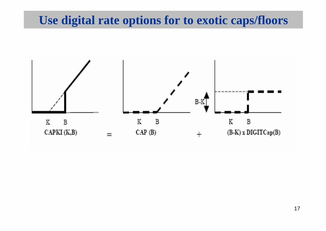
Use digital rate options for to exotic caps/floors
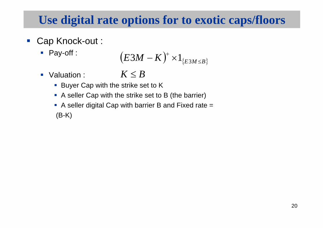
Cap Knock-in :Pay-off :
Valuation :Buyer Cap with the strike set to B (the barrier)A buyer digital “Cap” with barrier B and Fixed rate =
(B-K)
KB
KME BME313
17
Use digital rate options for to exotic caps/floors
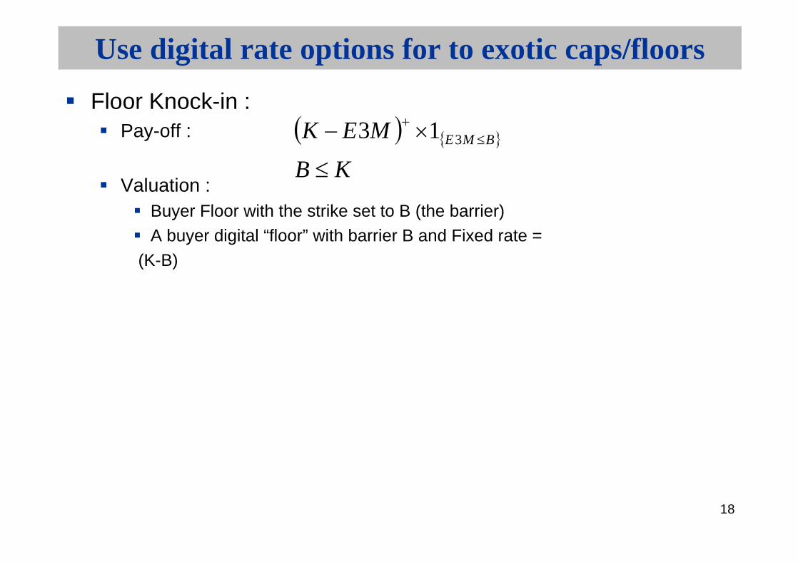
18
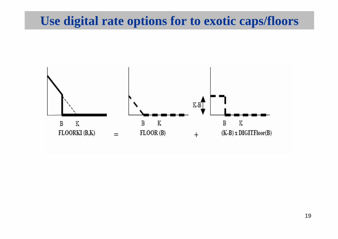
Use digital rate options for to exotic caps/floors
Floor Knock-in :Pay-off :
Valuation :Buyer Floor with the strike set to B (the barrier)A buyer digital “floor” with barrier B and Fixed rate =
(K-B)
KB
MEK BME313
19
Use digital rate options for to exotic caps/floors
20
Use digital rate options for to exotic caps/floors
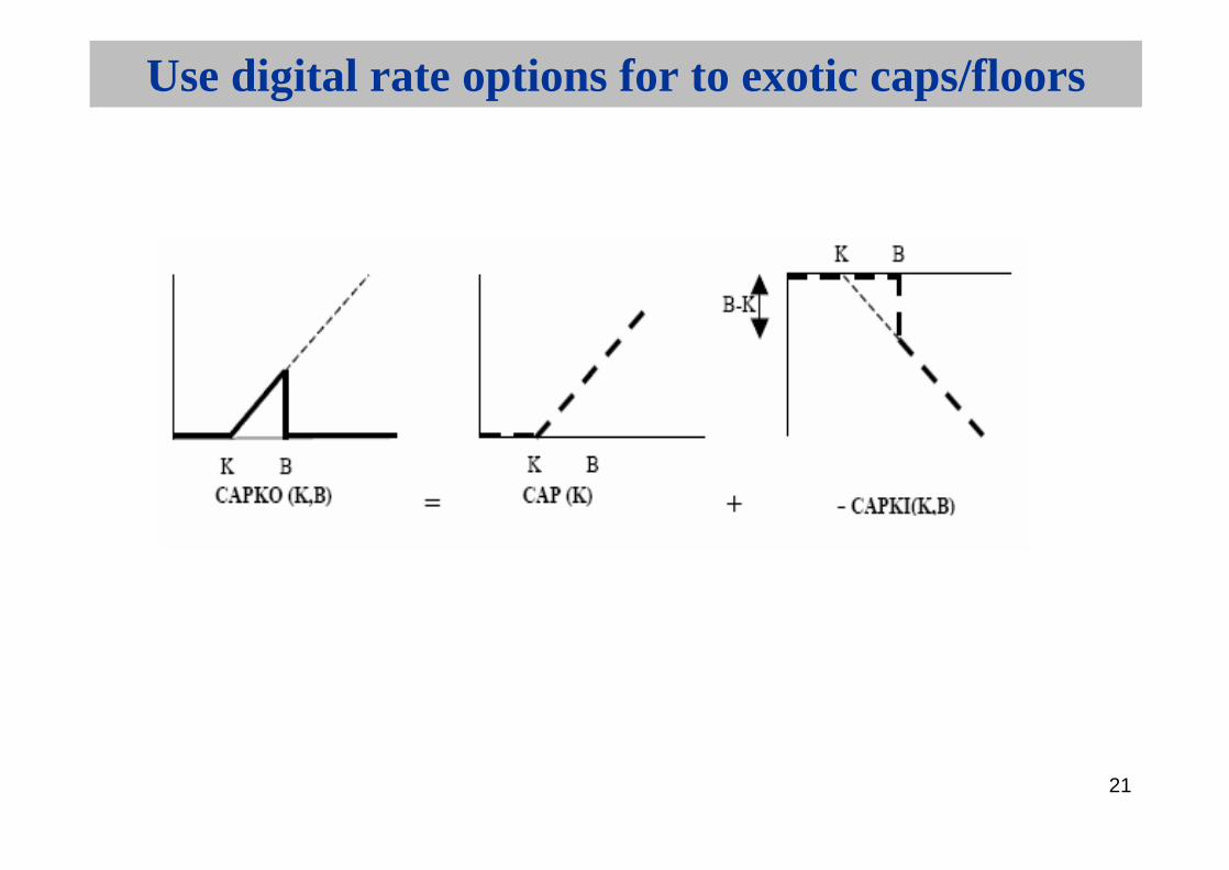
Cap Knock-out :Pay-off :
Valuation :Buyer Cap with the strike set to KA seller Cap with the strike set to B (the barrier)A seller digital Cap with barrier B and Fixed rate =
(B-K)
BK
KME BME313
21
Use digital rate options for to exotic caps/floors

22
Use digital rate options for swap KO
Swap KOBank pays
r if index1 < B, index2 + m otherwise
Replication of receiver swap KO:Receiver fixleg rate rPayer floatleg on index2Buyer cap Knock-In on index1
Buyer cap strike B on index1Buyer digital Cap barrier B on index1 and Fixed rate (B+m)-r

23
Digital rate options : application to exotic swaps
24
Digital rate options : application to exotic swaps
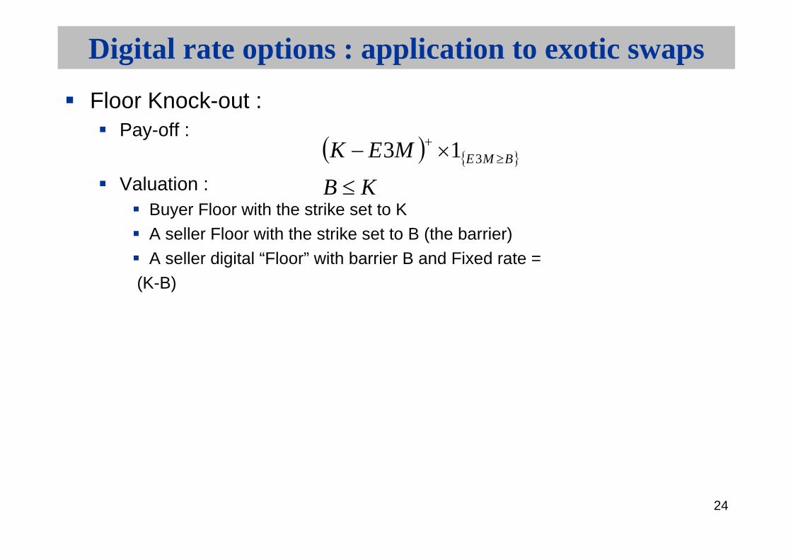
Floor Knock-out :Pay-off :
Valuation :Buyer Floor with the strike set to KA seller Floor with the strike set to B (the barrier)A seller digital “Floor” with barrier B and Fixed rate =
(K-B)
KB
MEK BME313

25
Digital rate options and applications to exotic swapsComplex Products : digital, steepner, ratchet…Bermuda swaptionsCallablesAppendixes :Standard Deviations vs VolatilitiesSABRCorrelation issuesLGMRisk-Management of exotics

26
Products based on digital on spread
Example 1 (4Y swap):Client receives 4.65%Pays Euribor3M +n/N*4.65%
n : number of days on the interest period where spread CMS10Y-CMS2Y < BN : number of days on the interest period
4Y swap at pricing date (march 2005) : 3%B = 0.9% year 1, 0.85% year2, 0.8% year3, 0.75% year1
Example 2 (15Y amortizing swap) : Client receives Euribor3MPays 1.9% If CMS10Y-CMS2Y > 0.70%, 4.95% otherwise
In both case :fixing of CMS is in arrearsClient is long digitals on CMS10Y-CMS2Y spread that pays above strike
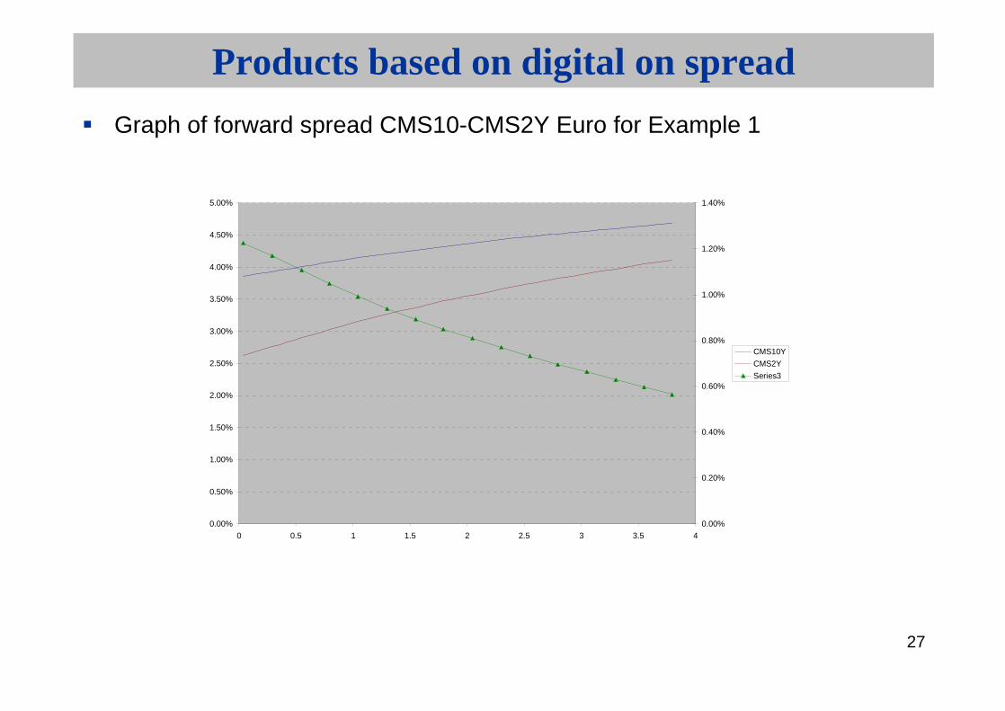
CMS10Y-2Y spread around 120/110 bp at pricing date
27
Products based on digital on spread
Graph of forward spread CMS10-CMS2Y Euro for Example 1
0.00%
0.50%
1.00%
1.50%
2.00%
2.50%
3.00%
3.50%
4.00%
4.50%
5.00%
0 0.5 1 1.5 2 2.5 3 3.5 4
0.00%
0.20%
0.40%
0.60%
0.80%
1.00%
1.20%
1.40%
CMS10Y
CMS2Y
Series3

28
Products based on digital on spread
Analysis :Both products were for debt liability managementStructured Swap enables the client to switch to fixed/float with enhanced rate if CMS10Y-CMS2Y spread stays above some barriers :
Client view on slope 10Y-2Y curve against the forward slopeRational : low spread = low growth + high inflation, high spread = higher growth + low inflationIssuance of debt + population ageing
Both product can be seen as vanilla swap + digitalAnalysis of the digitals
Sensitivity to the curve slopeFlattening of the curve implies higher probability of paying higher rates for the client, so client looses money on the swap
To analyze sensitivity to volatilities and correlation, let’s move to a basic model
29
Products based on digital on spread
The idea isWe know the basics of greeks on a single underlying digital, assuming this underlying normal or lognormalWhatever the model, it should have similar behaviour with respect to the parameters (volatilities or standard deviation + correlation)
Basic model to analyze a digital on CMS10Y-CMS2Y with maturity T :
Step 1 : Calculate CMS10Y(0,T) and CMS2Y(0,T) at date TStep 2 : calculate implied volatilities or better, implied standard deviation for ATM swaptions on 10Y and 2Y of maturity T
30
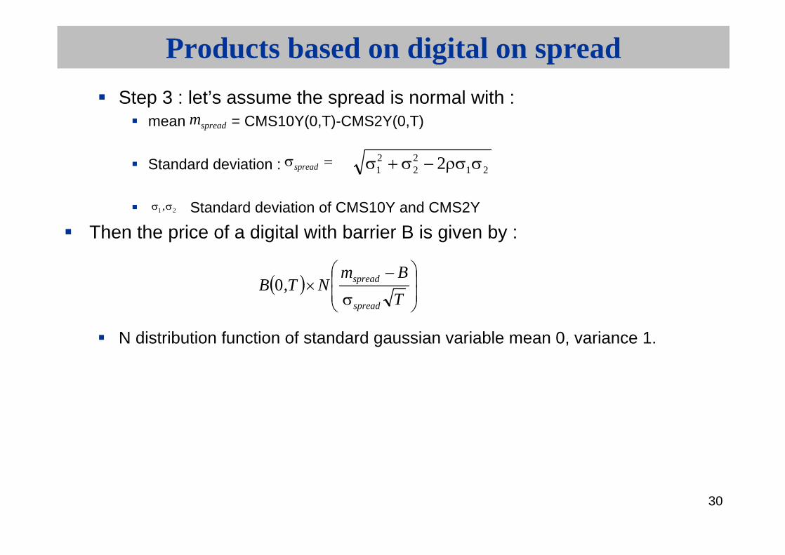
Products based on digital on spread
Step 3 : let’s assume the spread is normal with :mean = CMS10Y(0,T)-CMS2Y(0,T)
Standard deviation :
Standard deviation of CMS10Y and CMS2Y
Then the price of a digital with barrier B is given by :
N distribution function of standard gaussian variable mean 0, variance 1.
2122
21 2
21 ,
T
BmNT,B
spread
spread0
spreadm
spread

31
Products based on digital on spread
Basics behaviour of a digital with respect to the volatility (lognormal model) or the standard deviation (normal model) :
vega one year digital
-4
-3
-2
-1
0
1
2
3
60 70 80 90 100 110 120 130 140
spot
veg
a

32
Products based on digital on spread
To see the sensitivity to the standard deviation of each CMS, let’scalculate the derivative of the spread variance with respect to eachstandard deviation :
So even these derivatives are not obvious ; nevertheless, if the two standard deviation are close (usually it’s true) correlation not too high
Then, the standard deviation of the spread is increasing function of eachCMS standard deviationAnyway if both standard deviations increase, the standard deviation of the spread increaseStandard deviation of the spread is decreasing function of the correlation
2
12
2
2
1
21
1
2
1212 spreadspread ,
33
Products based on digital on spread
Digital vega of digital is positive out of the money, negative in the moneySo sensitivity of digital with respect to correlation and eachstandard deviation depends on moneyness
If you are long a digital that pays above the barrier, you are short volatility if forward spread above the strike, so long correlationIf you are long a digital that pays above the barrier, you are long volatilityif forward spread below the strike, so short correlation
Conclusion : The global sensitivities will depend mainly on each digital moneynessand marginally on the discount factors
to understand the various sensitivities always try first to go back to basics, i.e black& Scholes type models…

34
Products based on digital on spread
2005 story :Both Investors and liability management clients long digital that pays above the strikeFor investors, strikes generally below initial forwards spreads (long correlation)For Liability management, strikes generally above initial forwards spreads (short correlation)More risky position for liability management than for investors
LM clients buy digital out the money,Investors buy digital in the money
More products sold to investors, so banks were initially short correlation on digitals

35
Steepener
Typical steepener :Client receives 4*Max(CMS10Y-CMS2Y;0)Client long spread optionClient gains if slope increaseProducts stable with respect to a translation of the curveClient long the volatility of the spread, so short correlation
Banks can offset their short position on correlation due to digital by selling steepener

36
Other Complex products
RatchetsDefinition
The strike of the option or the coupon will depend on the preceding fixing. Common indexation is the following:
Coupon (i) = Notional * max (or min) [E6M(i) + T1; Coupon(i-1) + T2]First coupon is E6M observed at the start date + T1
Example :
Maturity 3Y; index E3M.Customer receives E3MCustomer pays E3M - 25 bps on the first coupon and then Max(E3M-25; Coupon(i-1))

37
Ratchets PricingVery path-dependent products.Main issue is to address the exposure to volatility at a strike that is not yet known. Vega exposure is more on local volatilities than on straight B&S volatilities.Need stochastic volatility model for pricing (same for vol bonds)
Ratchets Pricing useDifferent types that can match various strategies.In general, they are used when customer has a view on market beingeither stable or oriented with a strong, long-term trend. In case of strongmarket moves, they can lead to heavy losses.
Other Complex products

38
Ratchets second type (current version)Also different types that can match various strategies.
Example: Client pays E3M -0.30%+M, with margin M zero on the first year and afterwards previous margin + Max (0, 2%-E3M) It is a risky product.Similar to be short of floorlets strike 2% with cumulative effect in term of risk
There is no need of stochastic vol model, because the product is a series of puts, but one needs proper modeling for long delay adjustment. Ratchet cap or floor are both level and slope curves products
Other Complex products
39
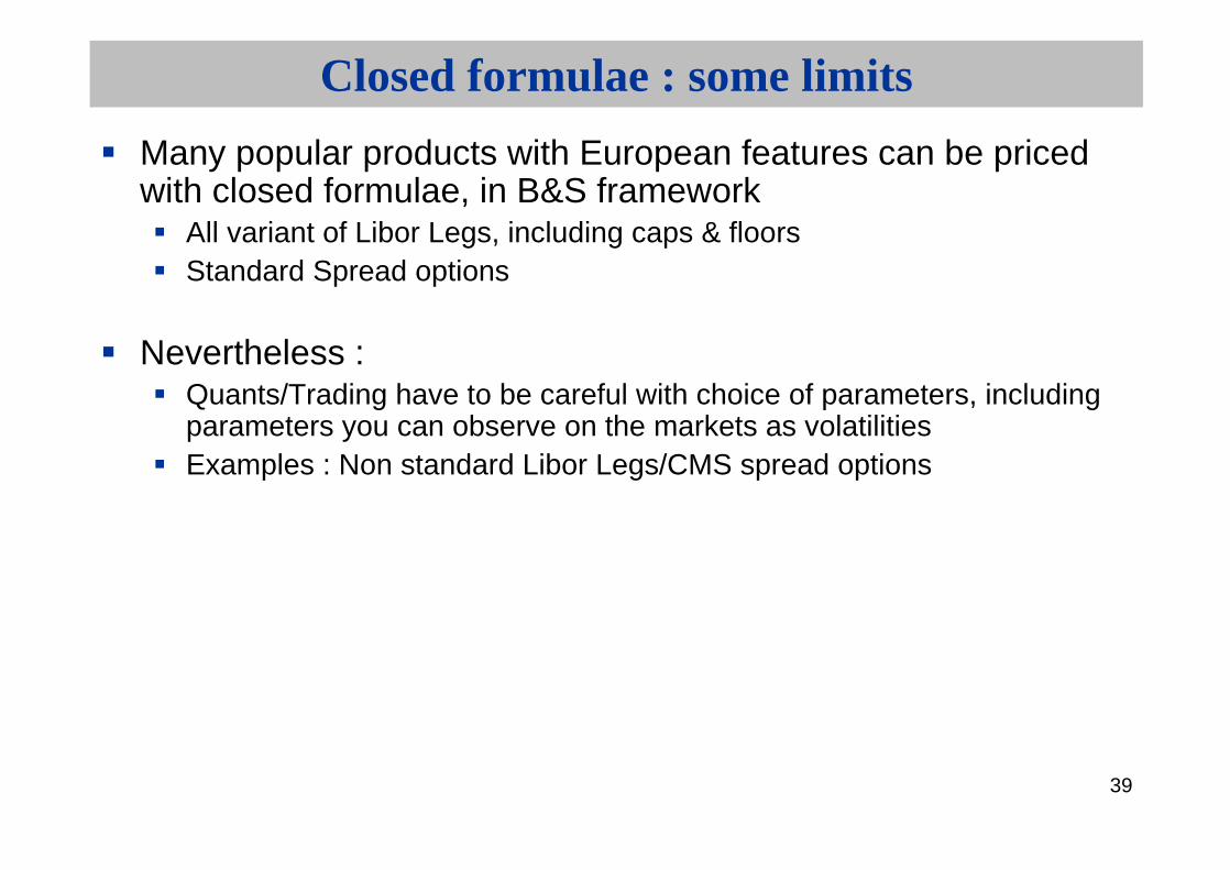
Closed formulae : some limits
Many popular products with European features can be priced with closed formulae, in B&S framework
All variant of Libor Legs, including caps & floorsStandard Spread options
Nevertheless :Quants/Trading have to be careful with choice of parameters, includingparameters you can observe on the markets as volatilitiesExamples : Non standard Libor Legs/CMS spread options
40
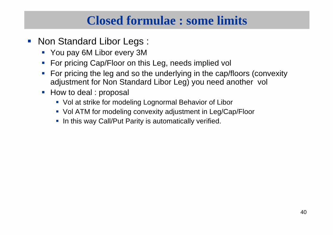
Closed formulae : some limits
Non Standard Libor Legs :You pay 6M Libor every 3MFor pricing Cap/Floor on this Leg, needs implied volFor pricing the leg and so the underlying in the cap/floors (convexity adjustment for Non Standard Libor Leg) you need another volHow to deal : proposal
Vol at strike for modeling Lognormal Behavior of LiborVol ATM for modeling convexity adjustment in Leg/Cap/FloorIn this way Call/Put Parity is automatically verified.

41
Closed formulae : some limits
CMS spread optionPay-off :Easy to calculate and compute closed formulae if both CMS assumed lognormal or normalWhich volatilities/standard deviations do take ?Main idea :
Volatilities must depend upon so that specific degenerated cases are consistently treated.We know the price of the spread option if maturity, one of the volatilities or one of the weights is zero.
maturitiesdifferent of being,)()( 2,12211 iCMSKTCMSmTCMSm
Kmm ,, 21
42
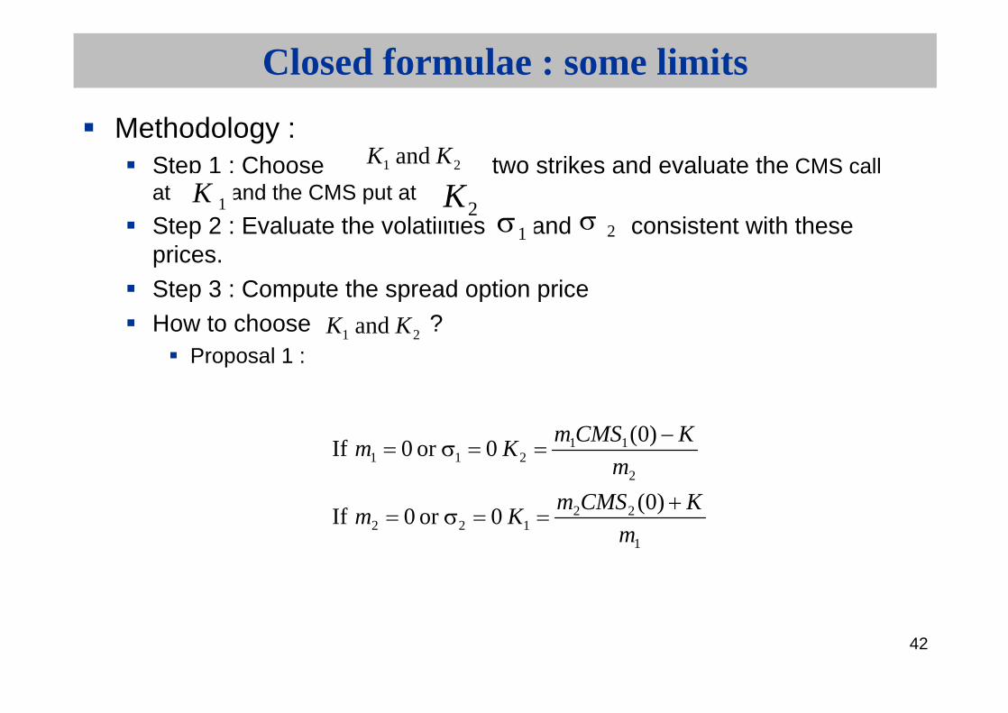
Closed formulae : some limits
Methodology : Step 1 : Choose two strikes and evaluate the CMS call at and the CMS put at
Step 2 : Evaluate the volatilities and consistent with these prices.Step 3 : Compute the spread option priceHow to choose ?
Proposal 1 :
21 and KK
1K2K
1 2
21 and KK
1
22122
2
11211
)0( 0or 0 If
)0( 0or 0 If
m
KCMSmKm
m
KCMSmKm

43
Closed formulae : some limitsProposal 2 :
with s standard deviations now
Best choice according to 2 dimensionnal gaussian law metricThis way stable pricing between normal or lognormal choice
2
112
1
221
)0(
)0(
m
KCMSmK
m
KCMSmK
)(),min(2)()(
),min(
)(),min(2)()(
),min(
2211211212
2221
211
221222222
2211211212
2221
211
22111111
KCMSmCMSmmmTTTmTm
mTTTmCMSK
KCMSmCMSmmmTTTmTm
mTTTmCMSK

44
Complex products
Bermuda Swaptions
Market conditions
The more competition you have between the included swaptions, the more expensive the bermuda.
- flat curve- in a steep curve:
The value of the bermuda is close to the value of the first swaption.This value can be increased thanks to a step up rate.
45
Other Complex products
FlexicapsThe buyer decides to be hedged on a limited number of fixings (1/2 usually).Either he decided himself when he wants the protection: liberty cap.Either it is automatic when the fixing is in the money: autocap.
46
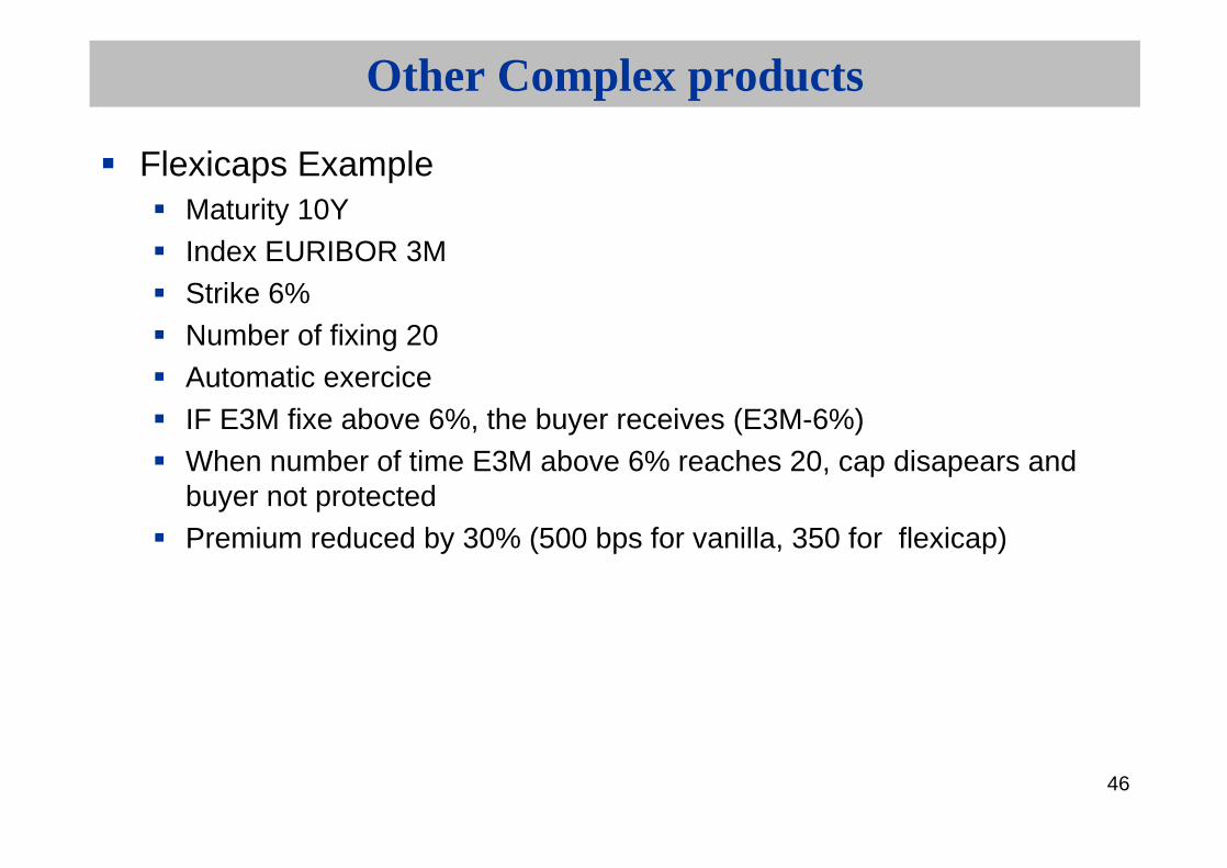
Other Complex products
Flexicaps ExampleMaturity 10YIndex EURIBOR 3MStrike 6%Number of fixing 20Automatic exerciceIF E3M fixe above 6%, the buyer receives (E3M-6%)When number of time E3M above 6% reaches 20, cap disapears and buyer not protectedPremium reduced by 30% (500 bps for vanilla, 350 for flexicap)
47
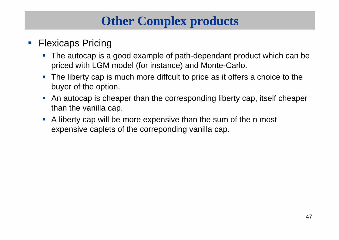
Other Complex products
Flexicaps PricingThe autocap is a good example of path-dependant product which can be priced with LGM model (for instance) and Monte-Carlo.The liberty cap is much more diffcult to price as it offers a choice to the buyer of the option.An autocap is cheaper than the corresponding liberty cap, itself cheaper than the vanilla cap.A liberty cap will be more expensive than the sum of the n most expensive caplets of the correponding vanilla cap.

48
Other Complex products
Flexicaps Use
Premium reductionA good product for a borrower who thinks a monetary crisis can occur but who believes these unlikely will not last for too long ( thanks to central banks).

49
Other Complex products
Flexicaps & Market conditions
Some conditions make them more attractive than vanilla caps:- a flat curve - high volatility- high correlation between forwards (if caps volatility are close to swaptions volatilities for example)
These parameters make them more likely to be in the money at the same time.
50
Other Complex products
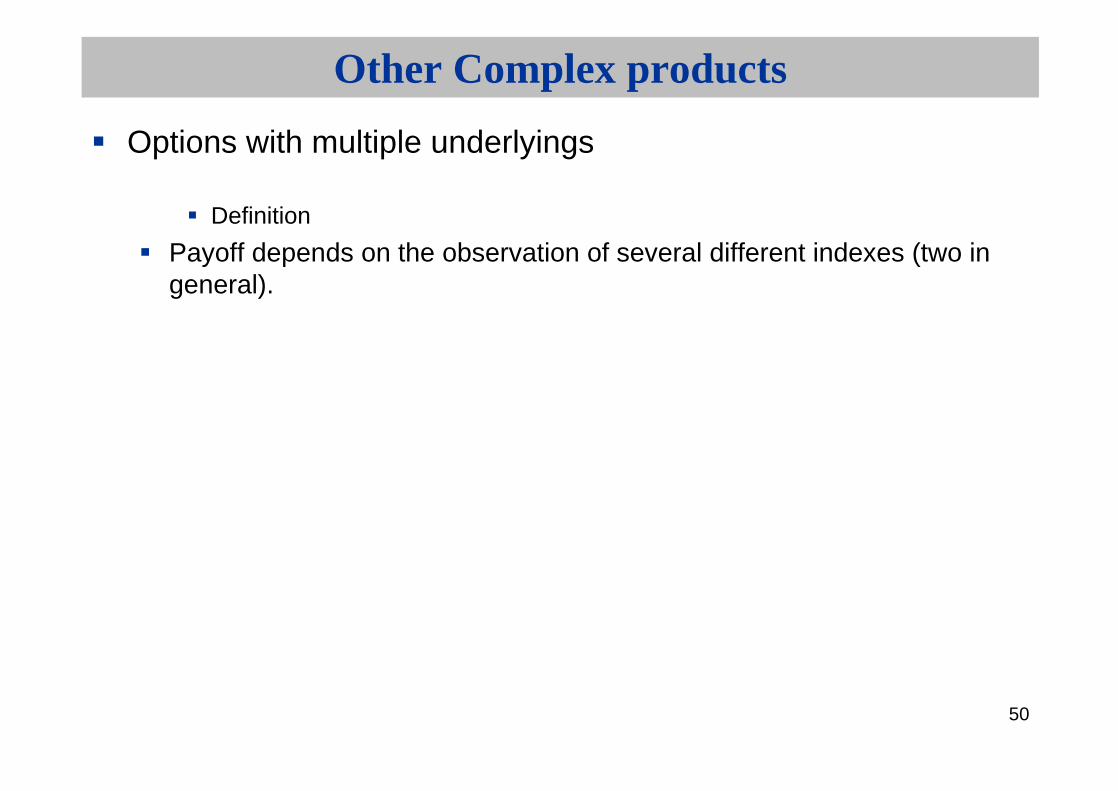
Options with multiple underlyings
Definition
Payoff depends on the observation of several different indexes (two in general).

51
Other Complex products
Options with multiple underlyings ExamplesThey can appear as the conditions of a range :
Range on a spread (customer bets on difference between Libor GBP and E3M being stable)Range with 2 conditions (bet on E3M staying within a range and 10Y swap, within another)
Or as options themselves :Call/Put on the spread on two short-term rates in two currenciesCall/Put on the spread between Long & Short Term rates in one currency (option on the slope of the curve)
Or as European Digitals : A Cap 5% on E3M Knock-Out on CMS10 being above 7% (fixing by fixing)

52
Other Complex products
Options with multiple underlying PricingThese products are priced with closed-formed formulas derived from B&S framework. Though, their pricing involves an crucial additional parameter : the correlation between the two indices.This correlation parameter can be determined as an implicit output of LGM model (for 2 indices of a same currency), or from historical data (for 2 currencies). Very few market prices can sometimes provide the implicit correlation priced by the market.

53
Other Complex products
Options with multiple underlying Use
Options with 2 indices in different currencies are mostly speculation tools as they can leverage a convergence strategy (ex : Forward Range on Stibor - Euribor)Options with 2 indices in the same currency can be used as speculation products too, but also as a balance sheet hedge tool. They are often used in EMTN on spreads, where coupon needs to befloored.

54
Other Complex products
Global Cap DefinitionA Global Cap is a protection on the total amount of interest paid on a debt.This can be seen as an option on the average of E3M
Example
Maturity 5Y; index E3M; strike 5.50%Premium = 160 bp, compared to 215 for vanilla cap (25% premium reduction)In 5 years, if the average of E3M has been below 5.50%, owner of the cap doesn’t receive any payoff, even if some fixings have been above 5.50%If the average of the fixings has been 6%, owner of the option will receive at maturity 0.50% * 5 *365 /360.
55
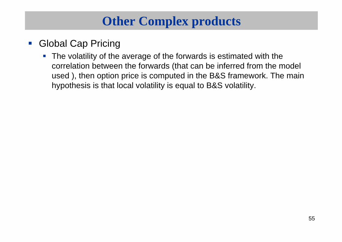
Other Complex products
Global Cap PricingThe volatility of the average of the forwards is estimated with the correlation between the forwards (that can be inferred from the model used ), then option price is computed in the B&S framework. The main hypothesis is that local volatility is equal to B&S volatility.
56
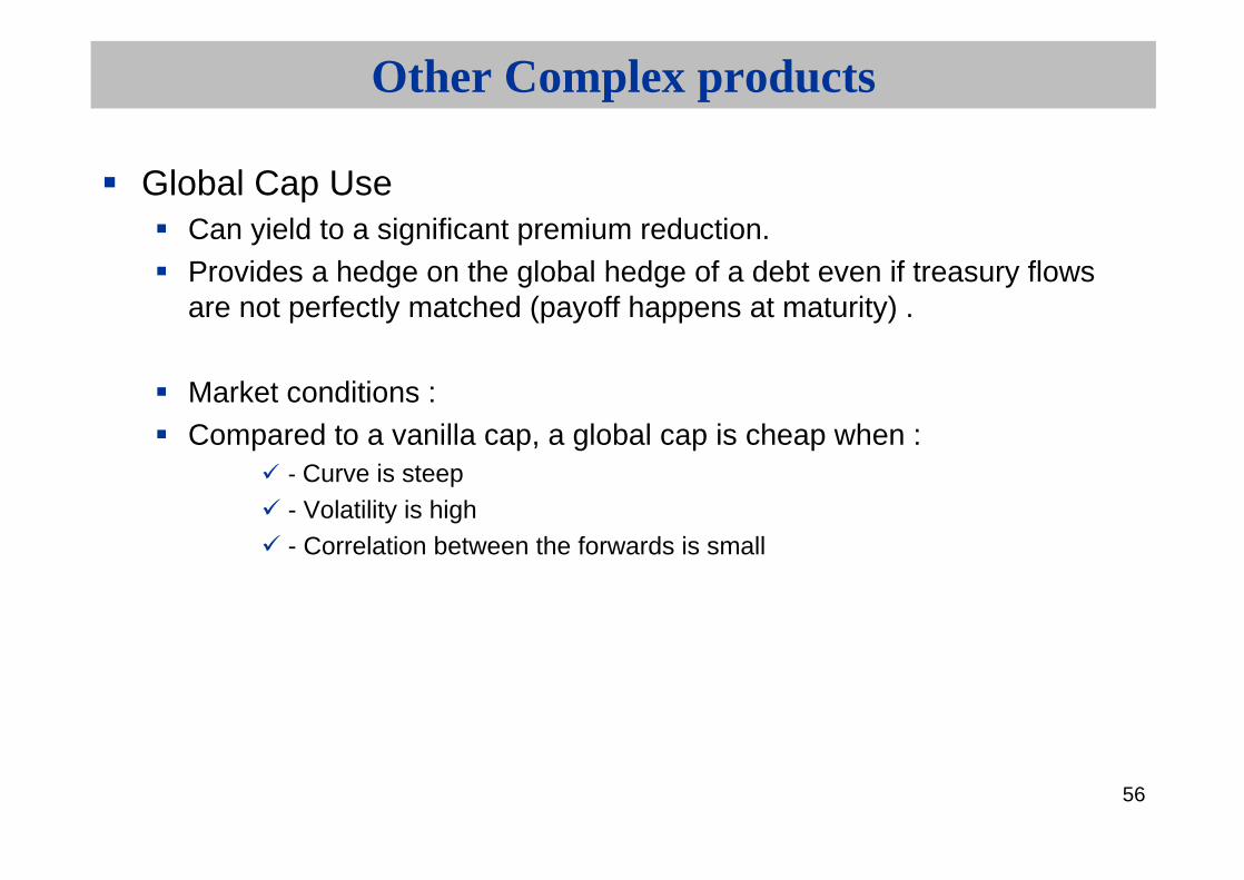
Other Complex products
Global Cap UseCan yield to a significant premium reduction.Provides a hedge on the global hedge of a debt even if treasury flows are not perfectly matched (payoff happens at maturity) .
Market conditions :Compared to a vanilla cap, a global cap is cheap when :
- Curve is steep
- Volatility is high- Correlation between the forwards is small

57
Other Complex products
Maturity CapAllows an financial institution to propose a floating rate loan while guaranteeing its customer that he won’t pay back his loan over more than a given period of time. In case capital has not been completely paid back after a given date, the seller of the option pays the remaining part of the debt.

58
Other Complex products
Example : Constant annuities are computed on a 15Y basis with a rate at 5.80%. If floating rates increase, each annuity will pay back less capital than forecasted (actually it can even not be enough to pay interest). The loan can then continue over an unlimited period of time. The ability to cap the maturity can be a marketing advantage.

59
Other Complex products
Maturity CapExample: Loan of 1MEUR on a 15Y basis at 5.80% semi-annually. Constant 6-month annuity is 50 365 EUR.The guarantee loan won’t go over 18 years is worth 150 bps flat, on 20 years it is worth 110 bps.

60
Digital rate options and applications to exotic swapsComplex Products : digital, steepner, ratchet…Bermuda swaptionsCallablesAppendixes :Standard Deviations vs VolatilitiesSABRCorrelation issuesLGMRisk-Management of exotics

61
Bermudas under LGM
Bermudan swaption: option to enter in a swap at severalexercise dates.
Bermuda Swaptions Utilization :
Bermuda swaptions are useful to hedge a callable paper or loan. They can also be packaged with a swap to get a callable swap. It gives a better rate than the boosted rate with a vanilla option.

62
Bermuda swaptions
Bermuda Swaptions
Pricing
PDE (Partial differential equation) or tree. At each nod of the tree, there will correspond an exercise date, the value of the option will be the max between the swap value and the value of the option itself.
Minimum value: a bermuda swaption is more expensive than the most expensive swaption included.Max value: the corresponding cap/floor. In our example, the bermuda is cheaper than the 9Y floor into 1Y 4.80%.

63
Bermudas under LGM
Calibration: One wants to be consistent with the market price of all underlyingswaptions, and especially with the most expensive ones.
Calibrate the diagonal of swaptions with strike the strike of the bermudan option.
64
Bermudas under LGM
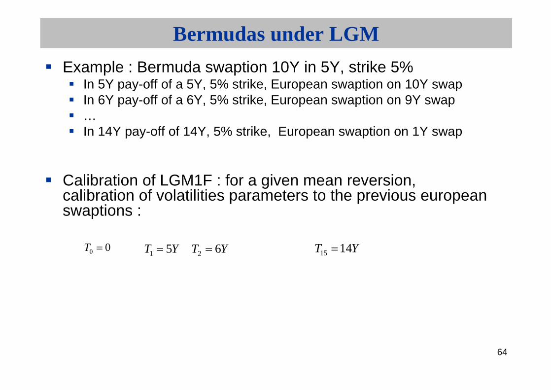
Example : Bermuda swaption 10Y in 5Y, strike 5%In 5Y pay-off of a 5Y, 5% strike, European swaption on 10Y swapIn 6Y pay-off of a 6Y, 5% strike, European swaption on 9Y swap…In 14Y pay-off of 14Y, 5% strike, European swaption on 1Y swap
Calibration of LGM1F : for a given mean reversion, calibration of volatilities parameters to the previous europeanswaptions :
00T YT 51 YT 62 YT 1415

65
Bermudas under LGM
constant between and constant between and
And so on…
Calibration of LGM2F is similar as again all parametersexcept volatilities are choosen and not part of the calibration.
1 0T 1T
2
1T2T

66
Bermudas under LGM
Exotic risk: To identify the part of « exotic » risk in the product (i.e. the riskorthogonal to the diagonal of swaptions), we use the followingdecomposition:
Bermuda = Most Expensive swaption + switch option
The most expensive swaption is, viewed from today, the one that is the most likely to be exercised.The switch option accounts for the future possibility to delay (or bring
forward) exercise, if it turns to be more interesting to do so.

67
Bermudas under LGM
Effect of mean reversion on bermuda prices
The switch option value is determined by the way the remainingswaptions are evaluated within the model, from each exercise date.
In other words, the parameters of interest are the model forwardvolatilities of remaining swap rates, computed from each exercise date. The larger the mean reversion, the larger these forward volatilities and thus the larger the price of the switch option.
68
Bermudas under LGM
The larger the mean reversion, the larger the price of the bermudanswaption.

69
Bermudas under LGM
Example : CASA USD deal as of 25/03/2003Deal characteristics : 30Y, no call 9Y. The bank pays fixed rate 6.65% quaterly 30/360 and receives LIBOR USD + 125 BP.
Notional = 650 Mios USD.Bermudan option price (3% mean reversion) :
5.51 % / 35.8 Mios USDCallable Swap (3% mean reversion) :
3.16 % / 20.5 Mios USD
mean reversion option structure
0.01 5.17% 2.82%
0.03 5.51% 3.16%
0.05 5.85% 3.50%

70
Bermudas under LGM
Most expensive (expiry = 9Y / term 21Y) = 4.34 % / 28.2 Mios USDSwitch option = bermudan option – most expensive = 1.17 % / 7.63 MiosUSDVega (1% parallel shift = 0.59 % / 3.87 Mios USD
71
Bermudas under LGM
Question: how to determine the mean reversion?
Market (e.g. on USD, for bermudas of short maturities).Statistical: use statistical methods to estimate the mean reversion fromthe short rate process itself (forget !) Historical vol of FRAs: compare historically the volatility of differentFRAs (e.g. 1Y vs. 20Y).

72
Bermudas under LGM
Long swaption vs. short swaption: each day, calibration to a long swaption. Choose the mean reversion so that, in average, short swaptions are well priced by the model.LGM forward vol vs. market vol: each day, calibrate to a diagonal of swaptions and, from the expiry of the most expensive, compare LGM forward vols of remaining swaptions, to the market (normal) volatilities of swaptions with same underlying / time to maturityBack testing: consider a Bermuda. Each day, and for several values of mean reversion, vega hedge the bermuda, delta hedge the overallposition and study the average / std deviation of daily P&L.

73
Bermudas under LGM
Historical study: long swaptions vs. short swaptions (or cap)Consider a set of historical datas (yield curves, vol curves)For each date, calibrate LGM to the diagonal of swaptions and determine the mean reversion such that the cap with same strike is well priced by the model
USD : mean reversion breakeven to match 10Y 5.00% Cap
2.00%
3.00%
4.00%
5.00%
6.00%
7.00%
May-03 Jul-03 Aug-03 Oct-03 Nov-03
EUR : mean reversion breakeven to match 10Y 4.50% Cap
2.00%
4.00%
6.00%
8.00%
10.00%
12.00%
Mar-03 May-03 Jun-03 Aug-03 Oct-03 Nov-03

74
Historical study: LGM forward vol vs. market volConsider a set of historical datas (yield curves, vol curves).At each date:
Calibrate the model to the diagonal of swaptions.
From the expiry date of the most expensive swaption, compute the normal LGM forward vols of all remaining swaptions.
Bermudas under LGM

75
Bermudas under LGM
Compare them to (normal) market volatilities of swaptions with same underlying & time to maturity.
Breakeven = mean reversion value such that the average of LGM forward vols matches the average of market normal vols.
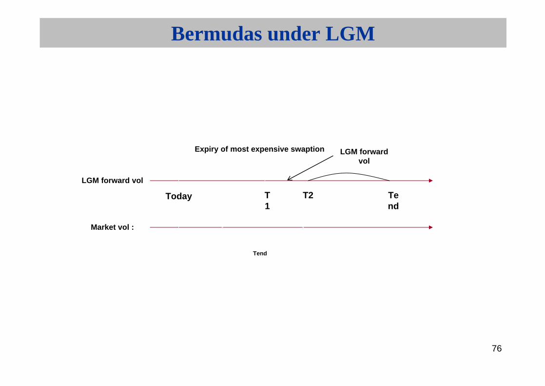
76
Bermudas under LGM
Today T1
T2 Tend
Expiry of most expensive swaption LGM forwardvol
T2 – T1 Tend – T2
LGM forward vol:
Market vol :
77
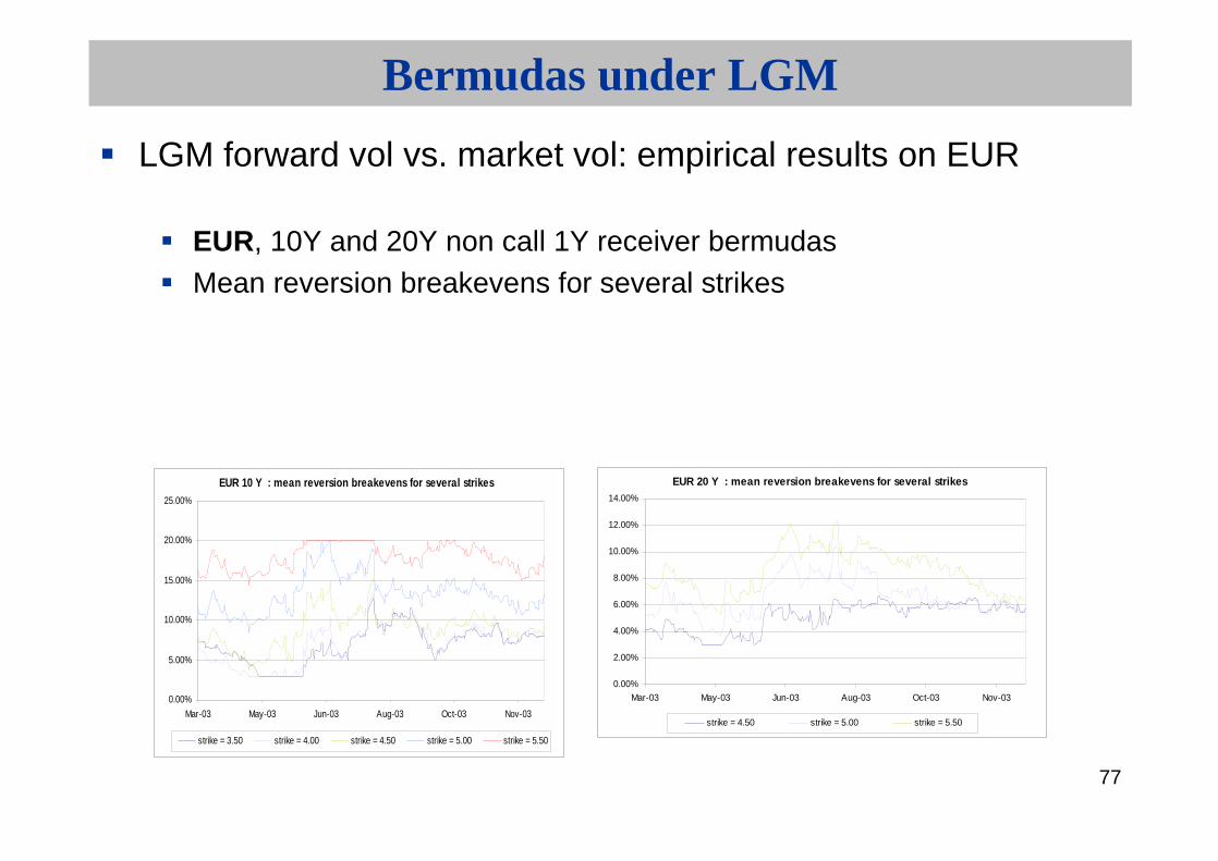
Bermudas under LGM
LGM forward vol vs. market vol: empirical results on EUR
EUR, 10Y and 20Y non call 1Y receiver bermudasMean reversion breakevens for several strikes
EUR 10 Y : mean reversion breakevens for several strikes
0.00%
5.00%
10.00%
15.00%
20.00%
25.00%
Mar-03 May-03 Jun-03 Aug-03 Oct-03 Nov-03
strike = 3.50 strike = 4.00 strike = 4.50 strike = 5.00 strike = 5.50
EUR 20 Y : mean reversion breakevens for several strikes
0.00%
2.00%
4.00%
6.00%
8.00%
10.00%
12.00%
14.00%
Mar-03 May-03 Jun-03 Aug-03 Oct-03 Nov-03
strike = 4.50 strike = 5.00 strike = 5.50

78
Bermudas under LGM
LGM forward vol vs. market vol: empirical results on USD
USD, 10Y and 20Y non call 1Y receiver bermudasMean reversion breakevens for several strikes
USD 10 Y : mean reversion breakevens for several strikes
5.00%
10.00%
15.00%
20.00%
25.00%
May-03 Jul-03 Aug-03 Oct-03 Nov-03
strike = 4.00 strike = 4.50 strike = 5.00 strike = 5.50 strike = 6.00
USD 20 Y : mean reversion breakevens for several strikes
5.00%
10.00%
15.00%
20.00%
25.00%
May-03 Jul-03 Aug-03 Oct-03 Nov-03
strike = 4.50 strike = 5.00 strike = 5.50 strike = 6.00

79
Bermudas under LGM
LGM forward vol vs. market vol: some conclusionsResults:
Slightly high mean reversion breakevens (up to 15 – 20%), especially on USDStrike dependent (especially for 10Y bermudas)Depends on maturity

80
Bermudas under LGM
What to conclude?Avoid being massively short of forward vol. If it is the case, be
conservative (i.e. use a mean reversion greater than 15%), or better, use a stochastic volatility model.
What if doing the same study with LGM 2 Factors?

81
Bermudas under LGM
Risk management back testingConsider a set of historical datas (yield curves, vol curves)Consider a bermuda. For each date of the data set, compute the vegahedge, delta hedge the overall position and compute the P&L at the end of the day.Repeat the operation for several values of mean reversion and compare the results it terms of average and standard deviation of the daily P&L.Try to identify robustness properties on the mean reversion.

82
Bermudas under LGM
25Y non call 5YAverage of daily P&LEUR historical datas
-20
-10
0
10
20
30
-5% 0% 5% 10% 15% 20% 25%
mean reversion
Ave
rag
e o
f d
aily
P&
L
15Y non call 3Y (2 call dates)Average of daily P&L
Simulated datas
-1.5
-1
-0.5
0
0.5
1
0% 5% 10% 15% 20% 25%
mean reversion
Ave
rag
e o
f d
aily
P&
L

83
Bermudas under LGM
LGM 1 Factor vs. LGM 2 FactorsQuestion: is a one factor model appropriate to price and risk manage bermudas? In other words: to what extent decorrelation between rates affects the price of a bermuda ?To understand the effects involved, let us consider a receiver bermuda with only 2 exercise dates:
TodayT2
Tend
Exercise in T1 Delay exercise toT2

84
Bermudas under LGM
The payoff of the bermuda at date T1 looks like:
85
Bermudas under LGM
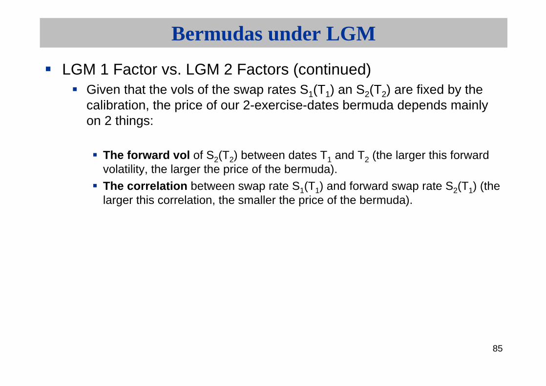
LGM 1 Factor vs. LGM 2 Factors (continued)Given that the vols of the swap rates S1(T1) an S2(T2) are fixed by the calibration, the price of our 2-exercise-dates bermuda depends mainlyon 2 things:
The forward vol of S2(T2) between dates T1 and T2 (the larger this forwardvolatility, the larger the price of the bermuda).The correlation between swap rate S1(T1) and forward swap rate S2(T1) (the larger this correlation, the smaller the price of the bermuda).
86
Bermudas under LGM
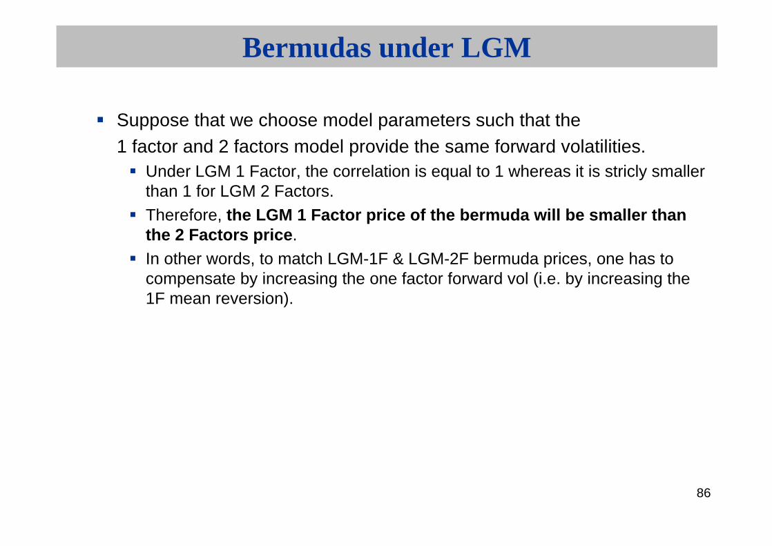
Suppose that we choose model parameters such that the 1 factor and 2 factors model provide the same forward volatilities.
Under LGM 1 Factor, the correlation is equal to 1 whereas it is stricly smallerthan 1 for LGM 2 Factors. Therefore, the LGM 1 Factor price of the bermuda will be smaller thanthe 2 Factors price.In other words, to match LGM-1F & LGM-2F bermuda prices, one has to compensate by increasing the one factor forward vol (i.e. by increasing the 1F mean reversion).
87
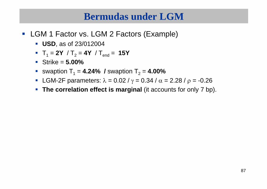
Bermudas under LGM
LGM 1 Factor vs. LGM 2 Factors (Example)USD, as of 23/012004T1 = 2Y / T2 = 4Y / Tend = 15YStrike = 5.00%swaption T1 = 4.24% / swaption T2 = 4.00%LGM-2F parameters: = 0.02 / = 0.34 / = 2.28 / = -0.26The correlation effect is marginal (it accounts for only 7 bp).

88
Bermudas under LGM
LGM-2F bermuda price = 5.17% , therefore switch option = 0.93% LGM-2F correlation S1(T1) / S2(T1) = 0.977LGM-1F mean reversion that matches 2F forward vol = 4.00%LGM-1 bermuda price for this mean reversion = 5.10%The conclusion holds for more than 2 exercise dates. On all exampleswe considered, the discrepancies remain below 10 bp.Basically, what matters is what happens around the most expensiveswaptions.

89
Conclusion / Summary
Bermuda = swaption + exotic risk (switch option)Exotic risk depends on forward volatilityUnder LGM, forward volatility depends on mean reversionMean reversion is chosen historically, using several approachesLGM one factor is appropriate for bermudasTypical mean reversion 1.5% to 5%, nearly market implied parameter

90
Amortizing bermudan swaptions
Standard diagonal calibration on vanilla swaptions is not satisfactory.Idea:
Swap with variable notional = basket of vanilla swaps with various end dates.

91
Amortizing bermudan swaptions
Example : a 3Y annual amortizing swap with notionals 2 mios EUR on first year, 1.5 mios EUR on second year, and 1 mios EUR on third year, is the sum of three vanilla swaps (3Y with notional 1 + 2Y with notional 0.5 + 1Y with notional 0.5) .
The idea is the following:For each exercise date, compute the basket of (forward) vanilla swaps equivalent to the (forward) amortizing swap.For each exercise date, consider the corresponding basket of swaptions (with same coefficients as in the basket of swaps), with strike the strike of the bermudan, and calibrate the model to the market price of this basket.
92
Amortizing bermudan swaptions
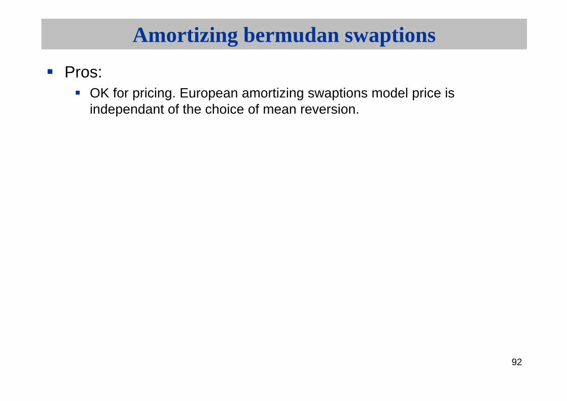
Pros:OK for pricing. European amortizing swaptions model price isindependant of the choice of mean reversion.

93
Amortizing bermudan swaptions
For hedging, the gamma replication may be inacurrate : as the swaptions of the basket have fixed strikes, there might be a mismatch between the gamma of the basket of swaptions and the gamma of the amortizingswaption, especially when the amortizing swaption turns to be ATM.
94
Bermuda swaptions aproximation
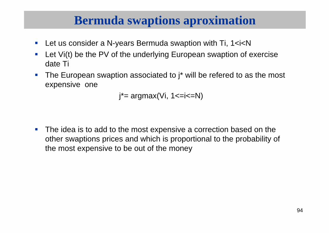
Let us consider a N-years Bermuda swaption with Ti, 1<i<NLet Vi(t) be the PV of the underlying European swaption of exercisedate TiThe European swaption associated to j* will be refered to as the mostexpensive one
j*= argmax(Vi, 1<=i<=N)
The idea is to add to the most expensive a correction based on the other swaptions prices and which is proportional to the probability of the most expensive to be out of the money
95
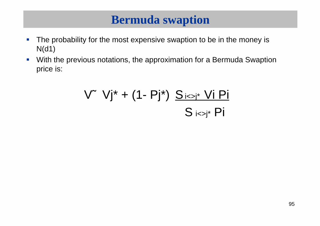
Bermuda swaption
The probability for the most expensive swaption to be in the money isN(d1)With the previous notations, the approximation for a Bermuda Swaptionprice is:
V˜ Vj* + (1- Pj*) S i<>j* Vi PiS i<>j* Pi

96
Digital rate options and applications to exotic swapsComplex Products : digital, steepner, ratchet…Bermuda swaptionsCallablesAppendixes :Standard Deviations vs VolatilitiesSABRCorrelation issuesLGMRisk-Management of exotics

97
Callables products
Bank pays 0.2% + (CMS20Y-CMS2Y)YENReceives Libor YEN6MCallable every 6 months after one yearAt every call date, after exchange of current cash flow
Bank PV = PV future cash flow + call option>=0Cancel option = Max(cancel at the current date, all future call)This is the decision rule between immediate cancel and keep the product Callable structures enable to create the possibility of pick-up for the client whicj is short the call option
98
Exotic products: definition
The main exotic feature of IR exotic products is their illiquidity: a lack of inter-bank market for the most exotic.
Most of them use non quoted parameters such as correlation.
These risks need a specific approach (“worst case”).
99
Exotic products: strategy
Importance of marketing: you need to identify a risk or an opportunity for a customer.
Being able to handle large volumes on vanilla products.
Strong interest of using historical data (for marketing and risk purposes) and a strong analysis of illiquid Greeks on illiquid risks.
Simulation of portfolio on different scenarios (VaR).

100
Exotic products : interest
To find the product which match the exact need and expectations of the customer.
In order to decrease the variance of a portfolio by accepting a lack in the expected return (more important bid/offer than the vanilla products).
And to minimize the future hedging cost.

101
Exotic products : non-hedgeable risk
Three kind of risk can be hedge with vanilla products :Parameters such as correlation between CMS, quanto correlationMean reversion if models use like for BermudaCorrelation between forward rates, model depending
No obvious solutionMeasure your risk wih good mappingLimit controlBuy and sell risk to stay within limits
102
Digital rate options and applications to exotic swapsComplex Products : digital, steepner, ratchet…Bermuda swaptionsCallablesAppendixes :Standard Deviations vs VolatilitiesSABRCorrelation issuesLGMRisk-Management of exotics

103
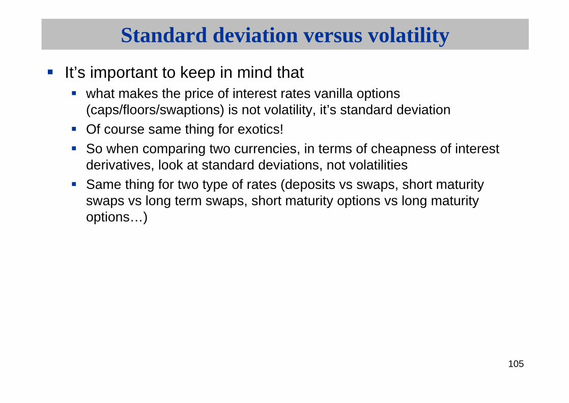
Standard deviation versus volatility
The diffusion process of a rate (short rate, zero-coupon, swap, whatever..) is typically :
dr = (…)dt + s dz (« normal models »), or dr/r = (…)dt + s ’dz (« lognormal models »)
It’s important to see the difference between s and s ’ : s is a standard deviation (often called volatility in working papers!)s ’ is a volatilty !

104
Standard deviation versus volatility
Central banks of developed countries tend to move short rates by 25 or 50 bp a few times in a year, whatever the level of short/long term rates
So standard deviation is typically 0.50% to 1.30%Volatility is very well approximated (ATM) by : s ’ = s /r(0)
r(0) initial value of r at date 0 Standard deviation is more stable across time for one currencySo volatility tends to increase when rates go down, tends to decrease when rates go-up
105
Standard deviation versus volatility
It’s important to keep in mind that what makes the price of interest rates vanilla options (caps/floors/swaptions) is not volatility, it’s standard deviationOf course same thing for exotics!So when comparing two currencies, in terms of cheapness of interest derivatives, look at standard deviations, not volatilitiesSame thing for two type of rates (deposits vs swaps, short maturity swaps vs long term swaps, short maturity options vs long maturity options…)
106
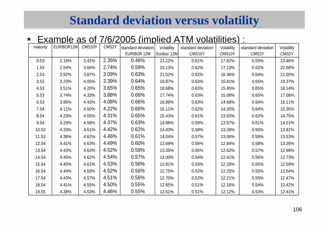
Standard deviation versus volatility
Example as of 7/6/2005 (implied ATM volatilities) :maturity EURIBOR12M CMS10Y CMS2Y
0.53 2.16% 3.41% 2.35% 0.46% 21.22% 0.61% 17.82% 0.55% 23.46%
1.53 2.54% 3.66% 2.74% 0.59% 23.13% 0.62% 17.13% 0.62% 22.58%
2.53 2.92% 3.87% 3.09% 0.63% 21.52% 0.62% 16.36% 0.64% 21.00%
3.53 3.23% 4.05% 3.39% 0.64% 19.87% 0.63% 15.81% 0.65% 19.37%
4.53 3.51% 4.20% 3.65% 0.65% 18.68% 0.63% 15.45% 0.65% 18.14%
5.53 3.74% 4.33% 3.88% 0.66% 17.74% 0.63% 15.08% 0.65% 17.08%
6.53 3.95% 4.43% 4.08% 0.66% 16.89% 0.63% 14.68% 0.64% 16.11%
7.54 4.11% 4.50% 4.22% 0.66% 16.11% 0.62% 14.30% 0.64% 15.35%
8.54 4.23% 4.55% 4.31% 0.65% 15.43% 0.61% 13.93% 0.62% 14.75%
9.54 4.29% 4.58% 4.37% 0.63% 14.86% 0.59% 13.57% 0.61% 14.21%
10.53 4.33% 4.61% 4.42% 0.62% 14.43% 0.58% 13.28% 0.60% 13.81%
11.53 4.38% 4.62% 4.46% 0.61% 14.04% 0.57% 13.06% 0.59% 13.53%
12.54 4.41% 4.63% 4.49% 0.60% 13.69% 0.56% 12.84% 0.58% 13.26%
13.54 4.43% 4.63% 4.52% 0.59% 13.35% 0.55% 12.62% 0.57% 12.98%
14.54 4.45% 4.62% 4.54% 0.57% 13.00% 0.54% 12.41% 0.56% 12.73%
15.54 4.45% 4.61% 4.53% 0.56% 12.81% 0.53% 12.29% 0.55% 12.59%
16.54 4.44% 4.59% 4.52% 0.56% 12.75% 0.52% 12.25% 0.55% 12.54%
17.54 4.43% 4.57% 4.51% 0.56% 12.70% 0.52% 12.21% 0.55% 12.47%
18.54 4.41% 4.55% 4.50% 0.55% 12.65% 0.51% 12.16% 0.54% 12.42%
19.55 4.38% 4.53% 4.46% 0.55% 12.61% 0.51% 12.12% 0.53% 12.41%
standard deviation CMS2Y
Volatility CMS2Y
standard deviation EURIBOR 12M
Volatility Euribor 12M
standard deviation CMS10Y
Volatility CMS10Y

107
Standard deviation versus volatility
0.00%
0.50%
1.00%
1.50%
2.00%
2.50%
3.00%
3.50%
4.00%
4.50%
5.00%
0 5 10 15 20 250.00%
5.00%
10.00%
15.00%
20.00%
25.00%
EURIBOR12M
CMS10Y
CMS2Y
standard deviation EURIBOR 12M
standard deviation CMS10Y
standard deviation CMS2Y
Volatility Euribor 12M
Volatility CMS10Y
Volatility CMS2Y
108
Standard deviation versus volatility
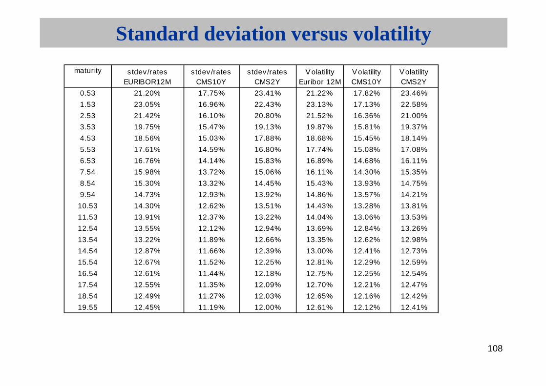
maturity
0.53 21.20% 17.75% 23.41% 21.22% 17.82% 23.46%
1.53 23.05% 16.96% 22.43% 23.13% 17.13% 22.58%
2.53 21.42% 16.10% 20.80% 21.52% 16.36% 21.00%
3.53 19.75% 15.47% 19.13% 19.87% 15.81% 19.37%
4.53 18.56% 15.03% 17.88% 18.68% 15.45% 18.14%
5.53 17.61% 14.59% 16.80% 17.74% 15.08% 17.08%
6.53 16.76% 14.14% 15.83% 16.89% 14.68% 16.11%
7.54 15.98% 13.72% 15.06% 16.11% 14.30% 15.35%
8.54 15.30% 13.32% 14.45% 15.43% 13.93% 14.75%
9.54 14.73% 12.93% 13.92% 14.86% 13.57% 14.21%
10.53 14.30% 12.62% 13.51% 14.43% 13.28% 13.81%
11.53 13.91% 12.37% 13.22% 14.04% 13.06% 13.53%
12.54 13.55% 12.12% 12.94% 13.69% 12.84% 13.26%
13.54 13.22% 11.89% 12.66% 13.35% 12.62% 12.98%
14.54 12.87% 11.66% 12.39% 13.00% 12.41% 12.73%
15.54 12.67% 11.52% 12.25% 12.81% 12.29% 12.59%
16.54 12.61% 11.44% 12.18% 12.75% 12.25% 12.54%
17.54 12.55% 11.35% 12.09% 12.70% 12.21% 12.47%
18.54 12.49% 11.27% 12.03% 12.65% 12.16% 12.42%
19.55 12.45% 11.19% 12.00% 12.61% 12.12% 12.41%
stdev/rates EURIBOR12M
stdev/rates CMS10Y
stdev/rates CMS2Y
V olatility Euribor 12M
Volatility CMS10Y
Volatility CMS2Y
109
Standard deviation versus volatility
8.00%
10.00%
12.00%
14.00%
16.00%
18.00%
20.00%
22.00%
24.00%
26.00%
0 5 10 15 20 25
stdev/rates EURIBOR12M
stdev/rates CMS10Y
stdev/rates CMS2Y
Volatility Euribor 12M
Volatility CMS10Y
Volatility CMS2Y

110
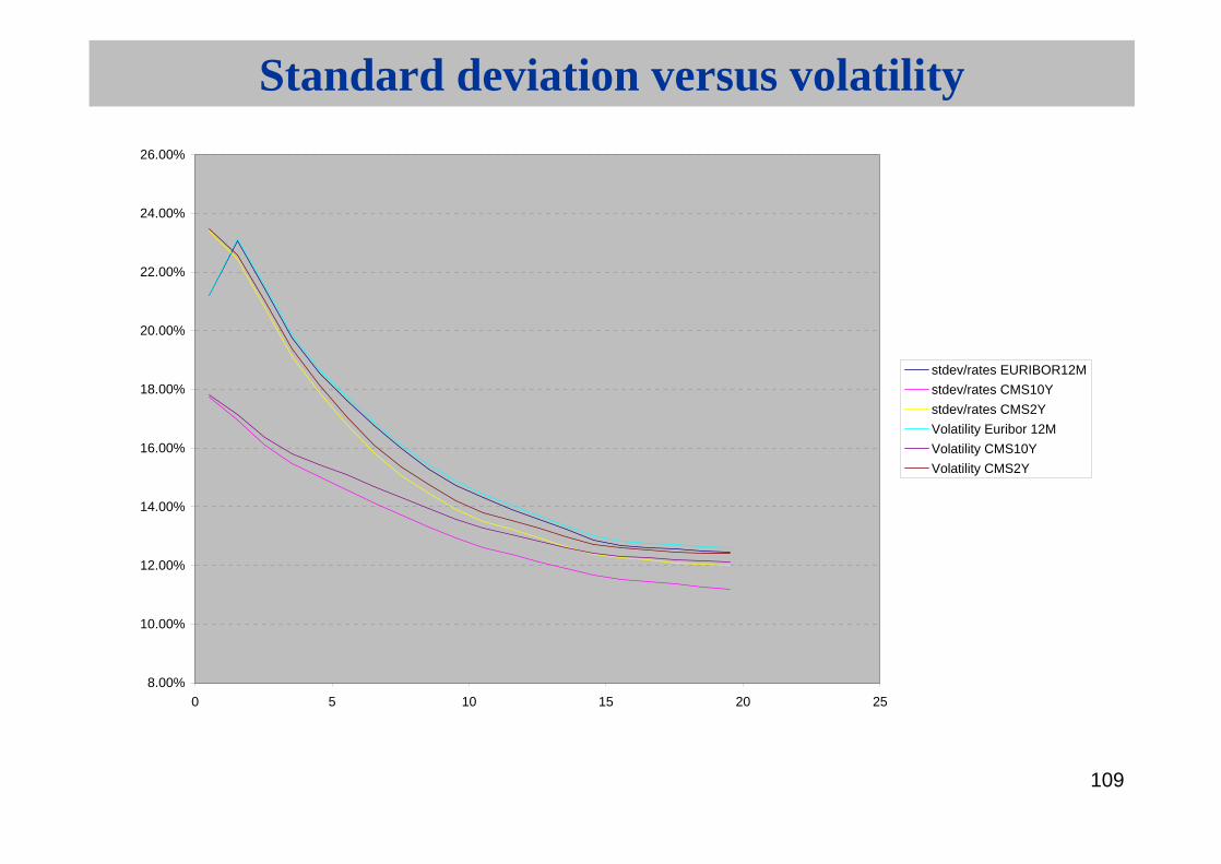
Standard deviation versus volatility
Remark : the approximation s ’ = s /r(0) is less good for CMS than for EURIBOR12M because implied volatilities were calculated before convexity adjustment.
111
Standard deviation versus volatility
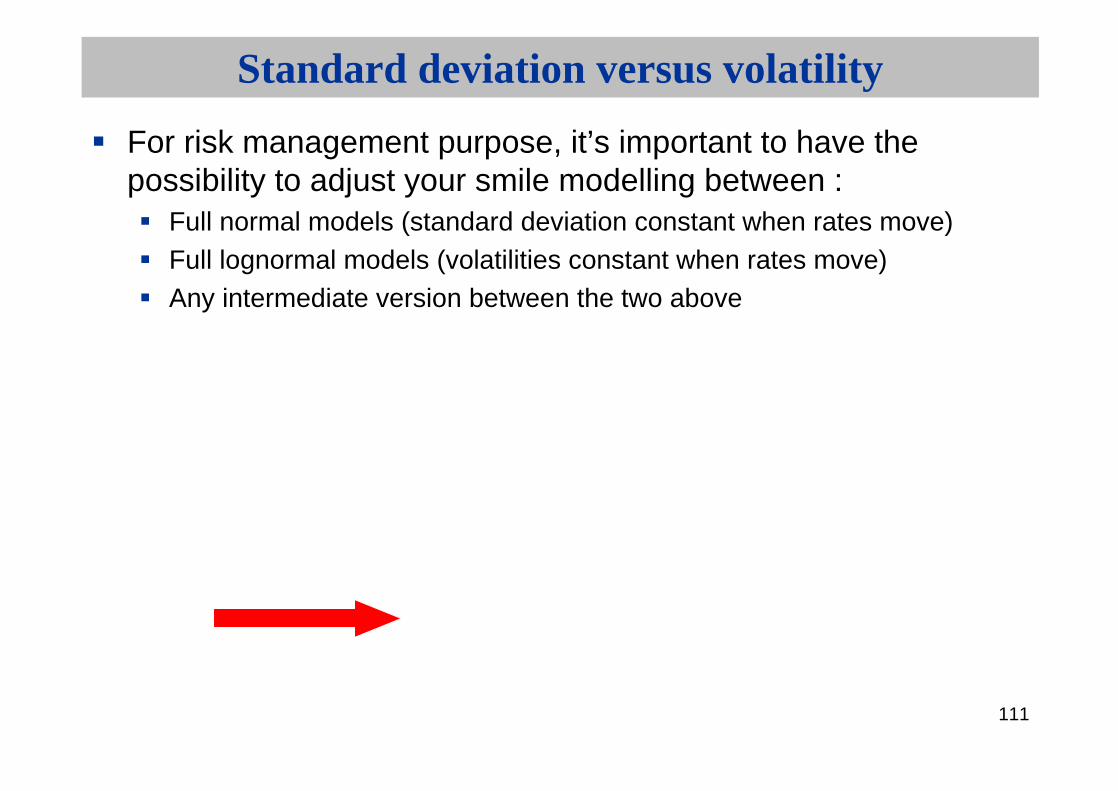
For risk management purpose, it’s important to have the possibility to adjust your smile modelling between :
Full normal models (standard deviation constant when rates move)Full lognormal models (volatilities constant when rates move)Any intermediate version between the two above
SABR model is a good choice

112
Digital rate options and applications to exotic swapsComplex Products : digital, steepner, ratchet…Bermuda swaptionsCallablesAppendixes :Standard Deviations vs VolatilitiesSABRCorrelation issuesLGMRisk-Management of exotics

113
SABR
SABR: Stochastic, Alpha, Beta, RhoDynamic of underlying :
with F forward rate or swap rate
dtdZdW
dZd
dWFdF
,
114
SABR
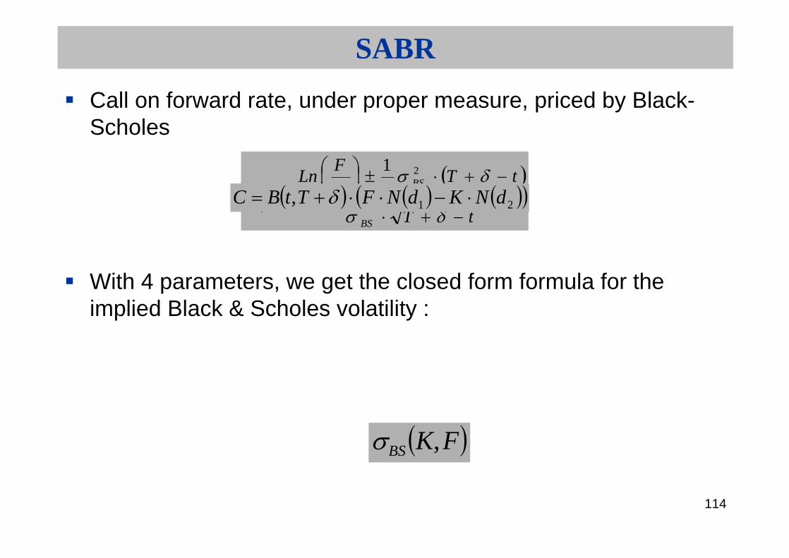
Call on forward rate, under proper measure, priced by Black-Scholes
With 4 parameters, we get the closed form formula for the implied Black & Scholes volatility :
tT
tTK
FLn
dBS
BS2
2,1
2
1
21, dNKdNFTtBC
FKBS ,

115
SABR
and
TFKFK
xy
x
K
F
K
FFK
FKBS
22
2
11
22
44
22
2
1
24
32
4
1
24
11
log19201
log24
11
,
1
21log
log
2
2
1
xxxxy
K
FFKx

116
SABR
At the money formula:
One can choose between parametrisation or replace by the ATM –normal or lognormal volatility.
TFFF
F,FBS2
2
122
22
1 24
32
4
1
24
11
,,,
117
SABR: the parameters
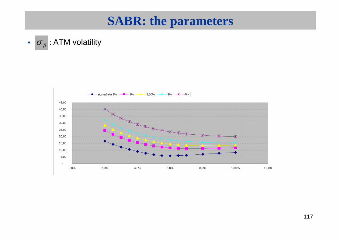
: ATM volatility
-
5,00
10,00
15,00
20,00
25,00
30,00
35,00
40,00
45,00
0,0% 2,0% 4,0% 6,0% 8,0% 10,0% 12,0%
sigmaBeta 1% 2% 2,50% 3% 4%

118
SABR: the parameters
BetaFor Beta=1, lognormal model.For beta = 0, normal model
Enables to know how ATM vol moves when forward moves.
F
dFd
ATM
ATM 1

119
For beta = 1, ATM vol doesn’t move when forward moves
SABR: the parameters
Beta = 1
20,00
20,50
21,00
21,50
22,00
22,50
23,00
23,50
24,00
24,50
25,00
0,0% 2,0% 4,0% 6,0% 8,0% 10,0% 12,0%
Fwd 3%
Fwd 4%
Fwd 5%
120
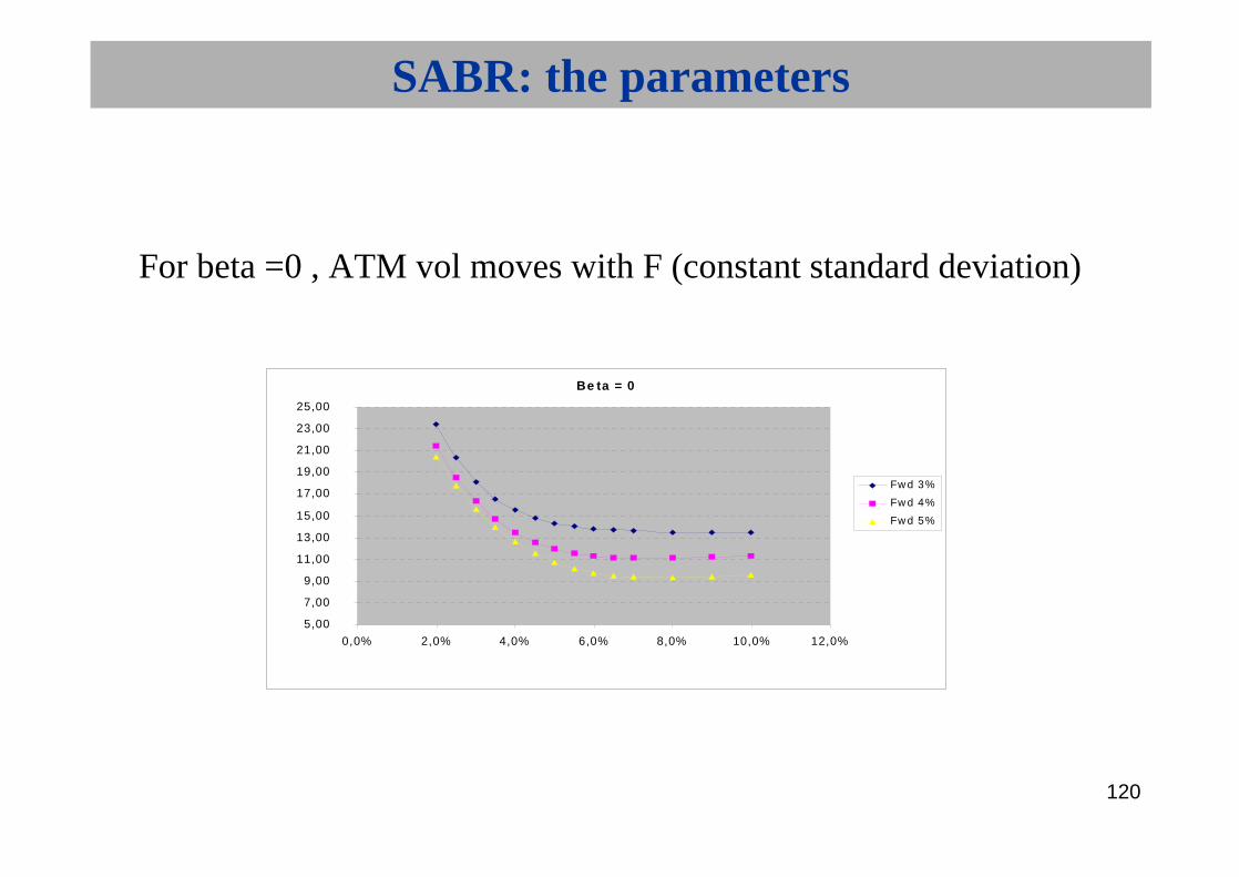
For beta =0 , ATM vol moves with F (constant standard deviation)
SABR: the parameters
Be ta = 0
5,00
7,00
9,00
11,00
13,00
15,00
17,00
19,00
21,00
23,00
25,00
0,0% 2,0% 4,0% 6,0% 8,0% 10,0% 12,0%
Fw d 3%
Fw d 4%
Fw d 5%
121
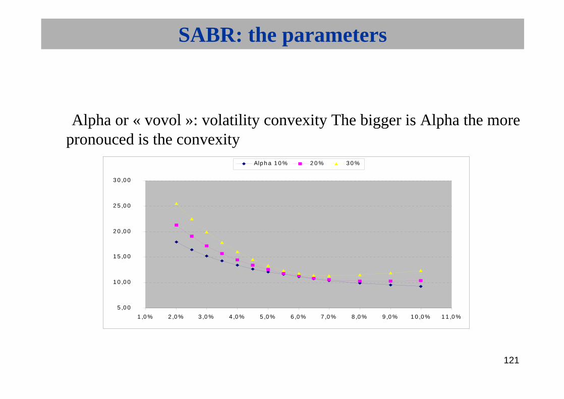
• Alpha or « vovol »: volatility convexity The bigger is Alpha the morepronouced is the convexity.
SABR: the parameters
5 ,0 0
1 0 ,0 0
1 5 ,0 0
2 0 ,0 0
2 5 ,0 0
3 0 ,0 0
1 ,0 % 2 ,0 % 3 ,0 % 4 ,0 % 5 ,0 % 6 ,0 % 7 ,0 % 8 ,0 % 9 ,0 % 1 0 ,0 % 1 1 ,0 %
Alp h a 1 0 % 2 0 % 3 0 %

122
• Rho : correlation between the volatility and the underlying causes whatwe call a Vanna skew : it’s the slope of the tangent line At the Money.
SABR: the parameters
10,00
12,00
14,00
16,00
18,00
20,00
22,00
24,00
26,00
28,00
30,00
1,0% 2,0% 3,0% 4,0% 5,0% 6,0% 7,0% 8,0% 9,0% 10,0% 11,0%
Rho 0,1 0 -0,2

123
SABR: risk management
Delta:
Different from classic delta ! Choose Beta to have stable hedge, so predict smile dynamic (trader work and skill !).Vega: it’s the sensivity of the price to change in the volatility.
F
BS
F
BS
F
C BS
BS
124
SABR: risk management
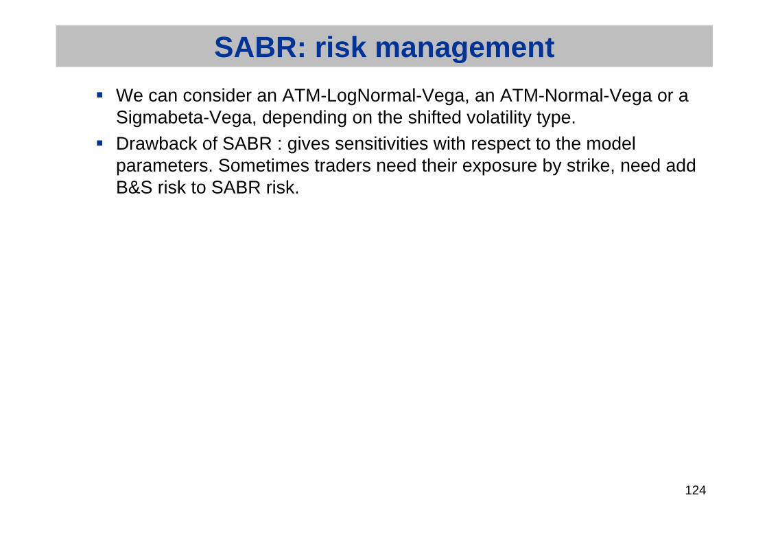
We can consider an ATM-LogNormal-Vega, an ATM-Normal-Vega or a Sigmabeta-Vega, depending on the shifted volatility type.Drawback of SABR : gives sensitivities with respect to the modelparameters. Sometimes traders need their exposure by strike, need add B&S risk to SABR risk.

125
SABR: risk managementVolga:
Hedged with strangles. If long vovol, buy straddle, sell strangle.
Vanna: qui ressemble à
hedged with collars.
C
F
C2 C

126
SABR : calibration
SABR model should provide a good fit to the observed implied volatility curves. Since SABR parameters have different and complementary effects on the smile, the calibration become easier and intuitive. Nevertheless, an exception has to be made for Beta and Rho. Indeed, those parameters have the same impact on the smile, and more precisely they both impact its skew.
Flndlnd ATM 1
127
SABR : calibration
To avoid over-parameterisation, the Beta is not calibrated but fixed from the smile rollNumerical calibration for other parameters

128
SABR : example : EUR 28/10/05S I G M A 1 M 3 M 6 M 1 Y 2 Y 3 Y 4 Y 5 Y 6 Y 7 Y 8 Y 9 Y 1 0 Y 1 5 Y 2 0 Y 2 5 Y 3 0 Y
1 M 1 . 2 3 % 1 . 1 8 % 1 . 3 0 % 2 . 0 3 % 2 . 5 5 % 2 . 5 4 % 2 . 5 3 % 2 . 5 2 % 2 . 4 4 % 2 . 3 7 % 2 . 3 3 % 2 . 2 9 % 2 . 2 6 % 2 . 1 0 % 2 . 0 5 % 2 . 0 0 % 1 . 9 7 %3 M 1 . 4 8 % 1 . 4 3 % 1 . 6 5 % 2 . 3 0 % 2 . 5 7 % 2 . 6 1 % 2 . 5 8 % 2 . 4 7 % 2 . 3 9 % 2 . 3 4 % 2 . 3 0 % 2 . 2 7 % 2 . 2 4 % 2 . 1 0 % 2 . 0 5 % 2 . 0 1 % 1 . 9 8 %6 M 1 . 9 3 % 1 . 8 8 % 2 . 1 2 % 2 . 3 4 % 2 . 5 8 % 2 . 5 4 % 2 . 5 0 % 2 . 4 6 % 2 . 3 9 % 2 . 3 3 % 2 . 2 9 % 2 . 2 7 % 2 . 2 5 % 2 . 0 9 % 2 . 0 4 % 1 . 9 9 % 1 . 9 7 %9 M 2 . 4 1 % 2 . 3 6 % 2 . 4 0 % 2 . 4 8 % 2 . 5 7 % 2 . 5 6 % 2 . 5 2 % 2 . 4 6 % 2 . 3 8 % 2 . 3 1 % 2 . 2 9 % 2 . 2 7 % 2 . 2 6 % 2 . 1 4 % 2 . 0 6 % 2 . 0 2 % 1 . 9 9 %1 Y 2 . 4 9 % 2 . 4 4 % 2 . 4 4 % 2 . 6 6 % 2 . 6 0 % 2 . 5 8 % 2 . 5 3 % 2 . 4 6 % 2 . 4 2 % 2 . 3 9 % 2 . 3 5 % 2 . 3 2 % 2 . 2 8 % 2 . 1 5 % 2 . 0 8 % 2 . 0 4 % 2 . 0 1 %2 Y 2 . 6 9 % 2 . 6 4 % 2 . 6 4 % 2 . 6 3 % 2 . 5 6 % 2 . 5 3 % 2 . 4 6 % 2 . 4 0 % 2 . 3 8 % 2 . 3 5 % 2 . 3 2 % 2 . 3 0 % 2 . 2 7 % 2 . 1 8 % 2 . 1 1 % 2 . 0 6 % 2 . 0 3 %3 Y 2 . 6 2 % 2 . 6 0 % 2 . 6 0 % 2 . 5 9 % 2 . 5 3 % 2 . 4 7 % 2 . 4 2 % 2 . 3 7 % 2 . 3 5 % 2 . 3 1 % 2 . 3 0 % 2 . 2 8 % 2 . 2 6 % 2 . 1 9 % 2 . 1 2 % 2 . 0 8 % 2 . 0 4 %4 Y 2 . 5 9 % 2 . 5 7 % 2 . 5 7 % 2 . 5 5 % 2 . 4 9 % 2 . 4 4 % 2 . 3 9 % 2 . 3 3 % 2 . 3 2 % 2 . 3 0 % 2 . 2 8 % 2 . 2 6 % 2 . 2 4 % 2 . 1 8 % 2 . 1 3 % 2 . 0 8 % 2 . 0 4 %5 Y 2 . 5 6 % 2 . 5 4 % 2 . 5 4 % 2 . 5 1 % 2 . 4 3 % 2 . 3 8 % 2 . 3 2 % 2 . 3 0 % 2 . 2 8 % 2 . 2 4 % 2 . 2 5 % 2 . 2 3 % 2 . 2 2 % 2 . 1 7 % 2 . 1 2 % 2 . 0 7 % 2 . 0 3 %
7 Y 2 . 4 5 % 2 . 4 4 % 2 . 4 4 % 2 . 3 9 % 2 . 2 9 % 2 . 2 6 % 2 . 2 1 % 2 . 2 0 % 2 . 1 9 % 2 . 1 6 % 2 . 1 7 % 2 . 1 6 % 2 . 1 5 % 2 . 1 1 % 2 . 0 6 % 2 . 0 2 % 1 . 9 8 %
1 0 Y 2 . 3 0 % 2 . 2 9 % 2 . 2 9 % 2 . 2 7 % 2 . 1 5 % 2 . 1 3 % 2 . 1 0 % 2 . 0 7 % 2 . 0 7 % 2 . 0 7 % 2 . 0 7 % 2 . 0 7 % 2 . 0 7 % 2 . 0 1 % 1 . 9 5 % 1 . 9 1 % 1 . 8 8 %
1 5 Y 2 . 0 6 % 2 . 0 4 % 2 . 0 4 % 2 . 0 2 % 1 . 9 4 % 1 . 9 2 % 1 . 9 1 % 1 . 8 9 % 1 . 8 9 % 1 . 9 0 % 1 . 9 0 % 1 . 9 0 % 1 . 9 1 % 1 . 8 5 % 1 . 7 9 % 1 . 7 4 % 1 . 7 2 %
2 0 Y 1 . 8 4 % 1 . 8 3 % 1 . 8 3 % 1 . 8 1 % 1 . 7 6 % 1 . 7 7 % 1 . 7 7 % 1 . 7 7 % 1 . 7 8 % 1 . 7 9 % 1 . 8 0 % 1 . 8 1 % 1 . 8 2 % 1 . 7 6 % 1 . 6 8 % 1 . 6 5 % 1 . 6 4 %
2 5 Y 1 . 7 6 % 1 . 7 4 % 1 . 7 4 % 1 . 7 2 % 1 . 6 9 % 1 . 7 0 % 1 . 7 1 % 1 . 7 2 % 1 . 7 3 % 1 . 7 4 % 1 . 7 5 % 1 . 7 6 % 1 . 7 7 % 1 . 7 1 % 1 . 6 6 % 1 . 6 4 % 1 . 6 3 %
3 0 Y 1 . 6 8 % 1 . 6 7 % 1 . 6 7 % 1 . 6 4 % 1 . 6 2 % 1 . 6 4 % 1 . 6 6 % 1 . 6 8 % 1 . 6 9 % 1 . 7 0 % 1 . 7 1 % 1 . 7 2 % 1 . 7 3 % 1 . 7 0 % 1 . 6 6 % 1 . 6 5 % 1 . 6 4 %
A L P H A 1 M 3 M 6 M 1 Y 2 Y 3 Y 4 Y 5 Y 6 Y 7 Y 8 Y 9 Y 1 0 Y 1 5 Y 2 0 Y 2 5 Y 3 0 Y
1 M 1 5 . 0 0 % 1 5 . 0 0 % 1 5 . 0 0 % 2 6 . 3 3 % 4 9 . 0 0 % 5 7 . 6 7 % 6 6 . 6 7 % 7 5 . 0 0 % 7 5 . 0 0 % 7 5 . 0 0 % 7 5 . 0 0 % 7 5 . 0 0 % 7 5 . 0 0 % 7 0 . 0 0 % 6 5 . 0 0 % 6 5 . 0 0 % 6 5 . 0 0 %
3 M 1 7 . 5 0 % 1 7 . 5 0 % 1 7 . 5 0 % 2 8 . 3 3 % 5 0 . 0 0 % 5 8 . 3 3 % 6 6 . 6 7 % 7 5 . 0 0 % 7 5 . 0 0 % 7 5 . 0 0 % 7 5 . 0 0 % 7 5 . 0 0 % 7 5 . 0 0 % 7 0 . 0 0 % 6 5 . 0 0 % 6 5 . 0 0 % 6 5 . 0 0 %
6 M 2 0 . 0 0 % 2 0 . 0 0 % 2 0 . 0 0 % 2 9 . 2 2 % 4 7 . 6 7 % 5 4 . 2 2 % 5 9 . 7 8 % 6 5 . 3 3 % 6 4 . 8 7 % 6 4 . 4 0 % 6 3 . 9 3 % 6 3 . 4 7 % 6 3 . 0 0 % 5 9 . 8 3 % 5 6 . 6 7 % 5 6 . 6 7 % 5 6 . 6 7 %
9 M 2 3 . 0 0 % 2 3 . 0 0 % 2 3 . 0 0 % 3 0 . 7 8 % 4 6 . 3 3 % 5 0 . 1 1 % 5 2 . 8 9 % 5 5 . 6 7 % 5 4 . 7 3 % 5 3 . 8 0 % 5 2 . 8 7 % 5 1 . 9 3 % 5 1 . 0 0 % 4 9 . 6 7 % 4 8 . 3 3 % 4 8 . 3 3 % 4 8 . 3 3 %
1 Y 3 4 . 0 0 % 3 4 . 0 0 % 3 4 . 0 0 % 3 8 . 0 0 % 4 6 . 0 0 % 4 6 . 0 0 % 4 6 . 0 0 % 4 6 . 0 0 % 4 4 . 6 0 % 4 3 . 2 0 % 4 1 . 8 0 % 4 0 . 4 0 % 3 9 . 0 0 % 3 9 . 5 0 % 4 0 . 0 0 % 4 0 . 0 0 % 4 0 . 0 0 %
2 Y 3 9 . 5 0 % 3 9 . 5 0 % 3 9 . 5 0 % 4 0 . 2 9 % 4 1 . 8 8 % 4 2 . 7 1 % 4 2 . 5 4 % 4 2 . 3 8 % 4 1 . 3 8 % 4 0 . 3 8 % 3 9 . 3 8 % 3 8 . 3 8 % 3 7 . 3 8 % 3 7 . 6 3 % 3 7 . 8 8 % 3 7 . 8 8 % 3 7 . 8 8 %
3 Y 4 1 . 5 0 % 4 1 . 5 0 % 4 1 . 5 0 % 4 0 . 5 8 % 3 8 . 7 5 % 3 9 . 4 2 % 3 9 . 0 8 % 3 8 . 7 5 % 3 8 . 1 5 % 3 7 . 5 5 % 3 6 . 9 5 % 3 6 . 3 5 % 3 5 . 7 5 % 3 5 . 7 5 % 3 5 . 7 5 % 3 5 . 7 5 % 3 5 . 7 5 %
4 Y 4 0 . 5 0 % 4 0 . 5 0 % 4 0 . 5 0 % 3 8 . 8 8 % 3 5 . 6 3 % 3 6 . 1 3 % 3 5 . 6 3 % 3 4 . 1 3 % 3 4 . 9 3 % 3 4 . 7 3 % 3 4 . 5 3 % 3 4 . 3 3 % 3 4 . 1 3 % 3 3 . 8 8 % 3 3 . 6 3 % 3 3 . 6 3 % 3 3 . 6 3 %
5 Y 3 7 . 0 0 % 3 7 . 0 0 % 3 7 . 0 0 % 3 5 . 8 3 % 3 3 . 5 0 % 3 2 . 8 3 % 3 2 . 1 7 % 3 1 . 5 0 % 3 1 . 7 0 % 3 1 . 9 0 % 3 2 . 1 0 % 3 2 . 3 0 % 3 2 . 5 0 % 3 2 . 0 0 % 3 1 . 5 0 % 3 1 . 5 0 % 3 1 . 5 0 %
7 Y 3 2 . 0 0 % 3 2 . 0 0 % 3 2 . 0 0 % 3 1 . 9 3 % 3 1 . 8 0 % 3 1 . 4 0 % 3 1 . 0 0 % 3 0 . 6 0 % 3 0 . 5 4 % 3 0 . 4 8 % 3 0 . 4 2 % 3 0 . 3 6 % 3 0 . 3 0 % 2 9 . 9 0 % 2 9 . 5 0 % 2 9 . 5 0 % 2 9 . 5 0 %
1 0 Y 2 8 . 5 0 % 2 8 . 5 0 % 2 8 . 5 0 % 2 8 . 7 5 % 2 9 . 2 5 % 2 9 . 2 5 % 2 9 . 2 5 % 2 9 . 2 5 % 2 8 . 8 0 % 2 8 . 3 5 % 2 7 . 9 0 % 2 7 . 4 5 % 2 7 . 0 0 % 2 6 . 7 5 % 2 6 . 5 0 % 2 6 . 5 0 % 2 6 . 5 0 %
1 5 Y 2 5 . 5 0 % 2 5 . 5 0 % 2 5 . 5 0 % 2 6 . 3 5 % 2 8 . 0 6 % 2 7 . 8 1 % 2 7 . 5 6 % 2 7 . 3 1 % 2 6 . 8 0 % 2 6 . 2 9 % 2 5 . 7 8 % 2 5 . 2 6 % 2 4 . 7 5 % 2 4 . 5 6 % 2 4 . 3 8 % 2 4 . 3 8 % 2 4 . 3 8 %
2 0 Y 2 5 . 0 0 % 2 5 . 0 0 % 2 5 . 0 0 % 2 5 . 6 3 % 2 6 . 8 8 % 2 6 . 3 8 % 2 5 . 8 8 % 2 5 . 3 8 % 2 4 . 8 0 % 2 4 . 2 3 % 2 3 . 6 5 % 2 3 . 0 8 % 2 2 . 5 0 % 2 2 . 3 8 % 2 2 . 2 5 % 2 2 . 2 5 % 2 2 . 2 5 %
2 5 Y 2 4 . 5 0 % 2 4 . 5 0 % 2 4 . 5 0 % 2 4 . 9 0 % 2 5 . 6 9 % 2 4 . 9 4 % 2 4 . 1 9 % 2 3 . 4 4 % 2 2 . 8 0 % 2 2 . 1 6 % 2 1 . 5 3 % 2 0 . 8 9 % 2 0 . 2 5 % 2 0 . 1 9 % 2 0 . 1 3 % 2 0 . 1 3 % 2 0 . 1 3 %
3 0 Y 2 4 . 0 0 % 2 4 . 0 0 % 2 4 . 0 0 % 2 4 . 1 7 % 2 4 . 5 0 % 2 3 . 5 0 % 2 2 . 5 0 % 2 1 . 5 0 % 2 0 . 8 0 % 2 0 . 1 0 % 1 9 . 4 0 % 1 8 . 7 0 % 1 8 . 0 0 % 1 8 . 0 0 % 1 8 . 0 0 % 1 8 . 0 0 % 1 8 . 0 0 %
R H O 1 M 3 M 6 M 1 Y 2 Y 3 Y 4 Y 5 Y 6 Y 7 Y 8 Y 9 Y 1 0 Y 1 5 Y 2 0 Y 2 5 Y 3 0 Y
1 M 3 3 . 0 0 % 3 3 . 0 0 % 3 3 . 0 0 % 3 3 . 6 7 % 3 5 . 0 0 % 3 0 . 0 0 % 2 5 . 0 0 % 2 0 . 0 0 % 1 8 . 0 0 % 1 6 . 0 0 % 1 4 . 0 0 % 1 2 . 0 0 % 1 0 . 0 0 % 5 . 2 5 % 0 . 5 0 % 0 . 5 0 % 0 . 5 0 %3 M 3 3 . 0 0 % 3 3 . 0 0 % 3 3 . 0 0 % 3 3 . 6 7 % 3 5 . 0 0 % 3 0 . 0 0 % 2 5 . 0 0 % 2 0 . 0 0 % 1 8 . 0 0 % 1 6 . 0 0 % 1 4 . 0 0 % 1 2 . 0 0 % 1 0 . 0 0 % 5 . 2 5 % 0 . 5 0 % 0 . 5 0 % 0 . 5 0 %6 M 3 3 . 0 0 % 3 3 . 0 0 % 3 3 . 0 0 % 3 2 . 5 6 % 3 1 . 6 7 % 2 7 . 0 0 % 2 2 . 3 3 % 1 7 . 6 7 % 1 1 . 3 0 % 9 . 6 0 % 7 . 9 0 % 6 . 2 0 % 8 . 1 7 % 1 . 2 5 % - 0 . 3 0 % - 3 . 5 0 % - 1 . 3 0 %9 M 3 3 . 0 0 % 3 3 . 0 0 % 3 3 . 0 0 % 3 1 . 4 4 % 2 8 . 3 3 % 2 4 . 0 0 % 1 9 . 6 7 % 1 5 . 3 3 % 1 1 . 3 0 % 9 . 6 0 % 7 . 9 0 % 6 . 2 0 % 6 . 3 3 % 1 . 2 5 % - 1 . 2 0 % - 3 . 5 0 % - 3 . 2 0 %1 Y 3 1 . 0 0 % 3 1 . 0 0 % 3 1 . 0 0 % 2 9 . 0 0 % 2 5 . 0 0 % 2 1 . 0 0 % 1 7 . 0 0 % 1 3 . 0 0 % 1 1 . 3 0 % 9 . 6 0 % 7 . 9 0 % 6 . 2 0 % 4 . 5 0 % 1 . 2 5 % - 2 . 0 0 % - 3 . 5 0 % - 5 . 0 0 %2 Y 2 3 . 0 0 % 2 3 . 0 0 % 2 3 . 0 0 % 2 2 . 5 8 % 2 1 . 7 5 % 1 7 . 4 2 % 1 3 . 0 8 % 8 . 7 5 % 7 . 3 8 % 6 . 0 0 % 4 . 6 3 % 3 . 2 5 % 1 . 8 8 % - 0 . 9 0 % - 3 . 8 0 % - 5 . 0 0 % - 6 . 3 0 %3 Y 2 0 . 5 0 % 2 0 . 5 0 % 2 0 . 5 0 % 1 9 . 8 3 % 1 8 . 5 0 % 1 3 . 8 3 % 9 . 1 7 % 4 . 5 0 % 3 . 4 5 % 2 . 4 0 % 1 . 3 5 % 0 . 3 0 % - 0 . 8 0 % - 3 . 1 0 % - 5 . 5 0 % - 6 . 5 0 % - 7 . 5 0 %4 Y 2 0 . 0 0 % 2 0 . 0 0 % 2 0 . 0 0 % 1 8 . 4 2 % 1 5 . 2 5 % 1 0 . 2 5 % 5 . 2 5 % 0 . 2 5 % - 0 . 5 0 % - 1 . 2 0 % - 1 . 9 0 % - 2 . 7 0 % - 3 . 4 0 % - 5 . 3 0 % - 7 . 3 0 % - 8 . 0 0 % - 8 . 8 0 %5 Y 2 0 . 0 0 % 2 0 . 0 0 % 2 0 . 0 0 % 1 7 . 3 3 % 1 2 . 0 0 % 6 . 6 7 % 1 . 3 3 % - 4 . 0 0 % - 4 . 4 0 % - 4 . 8 0 % - 5 . 2 0 % - 5 . 6 0 % - 6 . 0 0 % - 7 . 5 0 % - 9 . 0 0 % - 9 . 5 0 % - 1 0 . 0 0 %7 Y 2 0 . 0 0 % 2 0 . 0 0 % 2 0 . 0 0 % 1 6 . 1 5 % 8 . 4 4 % 3 . 8 9 % - 0 . 7 0 % - 5 . 2 0 % - 5 . 5 0 % - 5 . 8 0 % - 6 . 2 0 % - 6 . 5 0 % - 6 . 8 0 % - 8 . 3 0 % - 9 . 8 0 % - 1 0 . 3 0 % - 1 0 . 8 0 %
1 0 Y 1 8 . 5 0 % 1 8 . 5 0 % 1 8 . 5 0 % 1 3 . 3 7 % 3 . 1 0 % - 0 . 3 0 % - 3 . 6 0 % - 7 . 0 0 % - 7 . 2 0 % - 7 . 4 0 % - 7 . 6 0 % - 7 . 8 0 % - 8 . 0 0 % - 9 . 5 0 % - 1 1 . 0 0 % - 1 1 . 5 0 % - 1 2 . 0 0 %1 5 Y 1 3 . 0 0 % 1 3 . 0 0 % 1 3 . 0 0 % 9 . 4 4 % 2 . 3 3 % - 0 . 3 0 % - 3 . 6 0 % - 8 . 0 0 % - 7 . 2 0 % - 7 . 4 0 % - 7 . 6 0 % - 7 . 8 0 % - 9 . 9 0 % - 1 1 . 3 0 % - 1 2 . 6 0 % - 1 3 . 1 0 % - 1 3 . 5 0 %2 0 Y 7 . 0 0 % 7 . 0 0 % 7 . 0 0 % 5 . 1 8 % 1 . 5 5 % - 0 . 3 0 % - 3 . 6 0 % - 9 . 0 0 % - 7 . 2 0 % - 7 . 4 0 % - 7 . 6 0 % - 7 . 8 0 % - 1 1 . 8 0 % - 1 3 . 0 0 % - 1 4 . 3 0 % - 1 4 . 6 0 % - 1 5 . 0 0 %2 5 Y 3 . 0 0 % 3 . 0 0 % 3 . 0 0 % 2 . 2 6 % 0 . 7 8 % - 0 . 3 0 % - 3 . 6 0 % - 1 0 . 0 0 % - 7 . 2 0 % - 7 . 4 0 % - 7 . 6 0 % - 7 . 8 0 % - 1 3 . 6 0 % - 1 4 . 8 0 % - 1 5 . 9 0 % - 1 6 . 2 0 % - 1 6 . 5 0 %3 0 Y 1 . 0 0 % 1 . 0 0 % 1 . 0 0 % 0 . 6 7 % 0 . 0 0 % - 0 . 3 0 % - 3 . 6 0 % - 1 1 . 0 0 % - 7 . 2 0 % - 7 . 4 0 % - 7 . 6 0 % - 7 . 8 0 % - 1 5 . 5 0 % - 1 6 . 5 0 % - 1 7 . 5 0 % - 1 7 . 8 0 % - 1 8 . 0 0 %
B E T A 1 M 3 M 6 M 1 Y 2 Y 3 Y 4 Y 5 Y 6 Y 7 Y 8 Y 9 Y 1 0 Y 1 5 Y 2 0 Y 2 5 Y 3 0 Y1 M 0 . 4 0 . 4 0 . 4 0 . 4 0 . 4 0 . 4 0 . 4 0 . 4 0 . 4 0 . 4 0 . 4 0 . 4 0 . 4 0 . 4 0 . 4 0 . 4 0 . 43 M 0 . 4 0 . 4 0 . 4 0 . 4 0 . 4 0 . 4 0 . 4 0 . 4 0 . 4 0 . 4 0 . 4 0 . 4 0 . 4 0 . 4 0 . 4 0 . 4 0 . 46 M 0 . 4 0 . 4 0 . 4 0 . 4 0 . 4 0 . 4 0 . 4 0 . 4 0 . 4 0 . 4 0 . 4 0 . 4 0 . 4 0 . 4 0 . 4 0 . 4 0 . 49 M 0 . 4 0 . 4 0 . 4 0 . 4 0 . 4 0 . 4 0 . 4 0 . 4 0 . 4 0 . 4 0 . 4 0 . 4 0 . 4 0 . 4 0 . 4 0 . 4 0 . 41 Y 0 . 4 0 . 4 0 . 4 0 . 4 0 . 4 0 . 4 0 . 4 0 . 4 0 . 4 0 . 4 0 . 4 0 . 4 0 . 4 0 . 4 0 . 4 0 . 4 0 . 42 Y 0 . 4 0 . 4 0 . 4 0 . 4 0 . 4 0 . 4 0 . 4 0 . 4 0 . 4 0 . 4 0 . 4 0 . 4 0 . 4 0 . 4 0 . 4 0 . 4 0 . 43 Y 0 . 4 0 . 4 0 . 4 0 . 4 0 . 4 0 . 4 0 . 4 0 . 4 0 . 4 0 . 4 0 . 4 0 . 4 0 . 4 0 . 4 0 . 4 0 . 4 0 . 44 Y 0 . 4 0 . 4 0 . 4 0 . 4 0 . 4 0 . 4 0 . 4 0 . 4 0 . 4 0 . 4 0 . 4 0 . 4 0 . 4 0 . 4 0 . 4 0 . 4 0 . 45 Y 0 . 4 0 . 4 0 . 4 0 . 4 0 . 4 0 . 4 0 . 4 0 . 4 0 . 4 0 . 4 0 . 4 0 . 4 0 . 4 0 . 4 0 . 4 0 . 4 0 . 47 Y 0 . 4 0 . 4 0 . 4 0 . 4 0 . 4 0 . 4 0 . 4 0 . 4 0 . 4 0 . 4 0 . 4 0 . 4 0 . 4 0 . 4 0 . 4 0 . 4 0 . 4
1 0 Y 0 . 4 0 . 4 0 . 4 0 . 4 0 . 4 0 . 4 0 . 4 0 . 4 0 . 4 0 . 4 0 . 4 0 . 4 0 . 4 0 . 4 0 . 4 0 . 4 0 . 41 5 Y 0 . 4 0 . 4 0 . 4 0 . 4 0 . 4 0 . 4 0 . 4 0 . 4 0 . 4 0 . 4 0 . 4 0 . 4 0 . 4 0 . 4 0 . 4 0 . 4 0 . 42 0 Y 0 . 4 0 . 4 0 . 4 0 . 4 0 . 4 0 . 4 0 . 4 0 . 4 0 . 4 0 . 4 0 . 4 0 . 4 0 . 4 0 . 4 0 . 4 0 . 4 0 . 42 5 Y 0 . 4 0 . 4 0 . 4 0 . 4 0 . 4 0 . 4 0 . 4 0 . 4 0 . 4 0 . 4 0 . 4 0 . 4 0 . 4 0 . 4 0 . 4 0 . 4 0 . 43 0 Y 0 . 4 0 . 4 0 . 4 0 . 4 0 . 4 0 . 4 0 . 4 0 . 4 0 . 4 0 . 4 0 . 4 0 . 4 0 . 4 0 . 4 0 . 4 0 . 4 0 . 4
Vertical axis : maturity of option, Horizontal axis: underlying
129
SABR: conclusion and drawback
Good parametrisation of market smileEasy numerical calibrationParameters interpretation in term of risk-management
Main drawback : each underlying modeled separately :so can be inconsistent for some exotic productsmain application of risk-management is for vanilla products.

130
Digital rate options and applications to exotic swapsComplex Products : digital, steepner, ratchet…Bermuda swaptionsCallablesAppendixes :Standard Deviations vs VolatilitiesSABRCorrelation issuesLGMRisk-Management of exotics

131
Correlations issues
Example of correlation matrix : in red tenor, expiry = maturity of the options expiry 1y
3m 6m 1y 2y 5y 10y 15y 20y 30y3m 1.00 0.90 0.74 0.67 0.46 0.43 0.41 0.38 0.376m 0.90 1.00 0.79 0.71 0.49 0.44 0.42 0.38 0.381y 0.74 0.79 1.00 0.87 0.83 0.76 0.73 0.68 0.622y 0.67 0.71 0.87 1.00 0.89 0.86 0.79 0.72 0.695y 0.46 0.49 0.83 0.89 1.00 0.92 0.91 0.85 0.84
10y 0.43 0.44 0.76 0.86 0.92 1.00 0.93 0.90 0.8815y 0.41 0.42 0.73 0.79 0.91 0.93 1.00 0.92 0.9220y 0.38 0.38 0.68 0.72 0.85 0.90 0.92 1.00 0.9530y 0.37 0.38 0.62 0.69 0.84 0.88 0.92 0.95 1.00
expiry 2y3m 6m 1y 2y 5y 10y 15y 20y 30y
3m 1.00 0.92 0.79 0.73 0.57 0.54 0.53 0.50 0.506m 0.92 1.00 0.83 0.76 0.60 0.56 0.54 0.51 0.511y 0.79 0.83 1.00 0.89 0.85 0.79 0.77 0.73 0.662y 0.73 0.76 0.89 1.00 0.89 0.86 0.81 0.76 0.725y 0.57 0.60 0.85 0.89 1.00 0.92 0.91 0.88 0.87
10y 0.54 0.56 0.79 0.86 0.92 1.00 0.93 0.91 0.8915y 0.53 0.54 0.77 0.81 0.91 0.93 1.00 0.93 0.9320y 0.50 0.51 0.73 0.76 0.88 0.91 0.93 1.00 0.9530y 0.50 0.51 0.66 0.72 0.87 0.89 0.93 0.95 1.00
expiry 5y3m 6m 1y 2y 5y 10y 15y 20y 30y
3m 1.00 0.96 0.88 0.85 0.76 0.75 0.74 0.72 0.726m 0.96 1.00 0.91 0.87 0.79 0.77 0.76 0.74 0.741y 0.88 0.91 1.00 0.93 0.87 0.85 0.83 0.82 0.752y 0.85 0.87 0.93 1.00 0.89 0.87 0.85 0.82 0.785y 0.76 0.79 0.87 0.89 1.00 0.94 0.93 0.91 0.91
10y 0.75 0.77 0.85 0.87 0.94 1.00 0.95 0.93 0.9215y 0.74 0.76 0.83 0.85 0.93 0.95 1.00 0.95 0.9420y 0.72 0.74 0.82 0.82 0.91 0.93 0.95 1.00 0.9630y 0.72 0.74 0.75 0.78 0.91 0.92 0.94 0.96 1.00

132
Correlations issues
expiry 7y3m 6m 1y 2y 5y 10y 15y 20y 30y
3m 1.00 0.97 0.90 0.88 0.81 0.80 0.79 0.78 0.786m 0.97 1.00 0.93 0.89 0.83 0.82 0.81 0.80 0.791y 0.90 0.93 1.00 0.93 0.88 0.86 0.85 0.84 0.792y 0.88 0.89 0.93 1.00 0.89 0.87 0.85 0.84 0.815y 0.81 0.83 0.88 0.89 1.00 0.94 0.93 0.92 0.92
10y 0.80 0.82 0.86 0.87 0.94 1.00 0.95 0.94 0.9315y 0.79 0.81 0.85 0.85 0.93 0.95 1.00 0.96 0.9520y 0.78 0.80 0.84 0.84 0.92 0.94 0.96 1.00 0.9630y 0.78 0.79 0.79 0.81 0.92 0.93 0.95 0.96 1.00
expiry 10y3m 6m 1y 2y 5y 10y 15y 20y 30y
3m 1.00 0.98 0.91 0.90 0.83 0.82 0.81 0.80 0.806m 0.98 1.00 0.94 0.91 0.85 0.84 0.83 0.82 0.821y 0.91 0.94 1.00 0.94 0.88 0.87 0.86 0.85 0.822y 0.90 0.91 0.94 1.00 0.89 0.87 0.86 0.85 0.835y 0.83 0.85 0.88 0.89 1.00 0.94 0.93 0.93 0.93
10y 0.82 0.84 0.87 0.87 0.94 1.00 0.95 0.94 0.9315y 0.81 0.83 0.86 0.86 0.93 0.95 1.00 0.96 0.9520y 0.80 0.82 0.85 0.85 0.93 0.94 0.96 1.00 0.9630y 0.80 0.82 0.82 0.83 0.93 0.93 0.95 0.96 1.00
133
Correlations issues
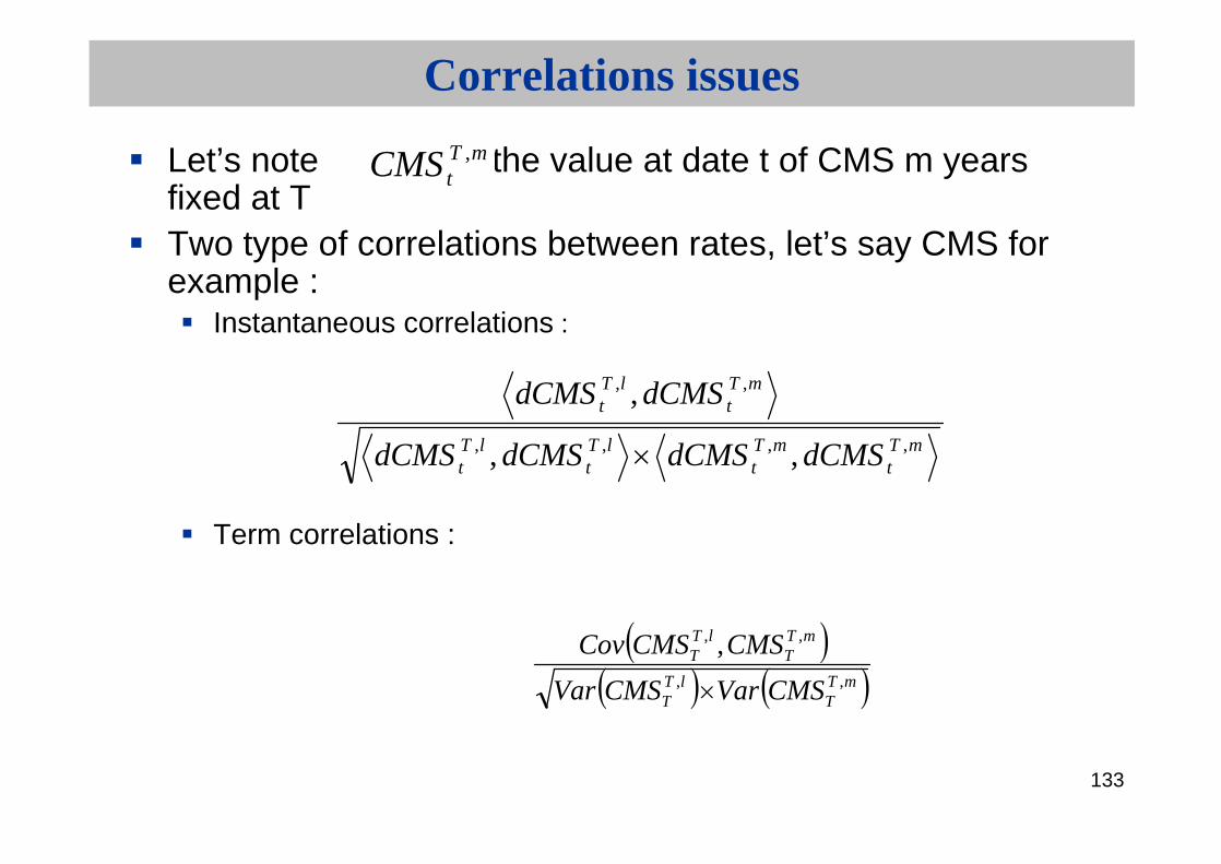
Let’s note the value at date t of CMS m yearsfixed at TTwo type of correlations between rates, let’s say CMS for example :
Instantaneous correlations :
Term correlations :
mTtCMS ,
mTt
mTt
lTt
lTt
mTt
lTt
dCMSdCMSdCMSdCMS
dCMSdCMS
,,,,
,,
,,
,
mTT
lTT
mTT
lTT
CMSVarCMSVar
CMSCMSCov,,
,, ,
134
Correlations issues
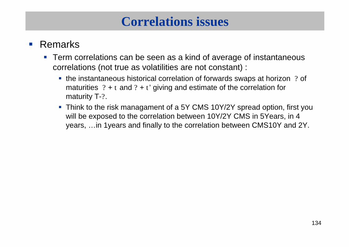
RemarksTerm correlations can be seen as a kind of average of instantaneouscorrelations (not true as volatilities are not constant) :
the instantaneous historical correlation of forwards swaps at horizon ? of maturities ? + t and ? + t ’ giving and estimate of the correlation for maturity T-?.Think to the risk managament of a 5Y CMS 10Y/2Y spread option, first youwill be exposed to the correlation between 10Y/2Y CMS in 5Years, in 4 years, …in 1years and finally to the correlation between CMS10Y and 2Y.

135
Correlations issues
For derivatives pricing/risk management (example : spreadoptions pricing), of course only term correlations are relevant.
136
Correlations issues
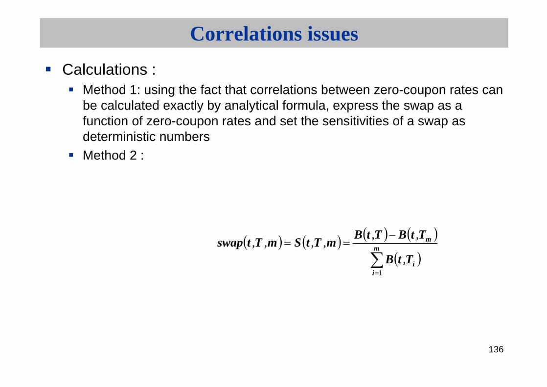
Calculations : Method 1: using the fact that correlations between zero-coupon rates canbe calculated exactly by analytical formula, express the swap as a function of zero-coupon rates and set the sensitivities of a swap as deterministic numbersMethod 2 :
m
ii
m
TtB
TtBTtBmTtSmTtswap
1
,
,,,,,,

137
Correlations issues in LGM2F
A sketch of calculations :
22
11 tt dWTtBTtdWTtBTtTtdB ,,,,,
22
11 tmmtmmm dWTtBTtdWTtBTtTtdB ,,,,,
222
111
tmm
tmmm
dWTtBTtTtBTt
dWTtBTtTtBTtTtBTtBd
,,,,
,,,,,,

138
Correlations issues in LGM2F
2
1
12
22
1
1
11
11
tm
ii
m
iii
m
mm
tm
ii
m
iii
m
mm
dWTtB
TtBTt
TtBTtBTtBTtTtBTt
dWTtB
TtBTt
TtBTtB
TtBTtTtBTt
mTtSmTtdS
,
,,
,,
,,,,
,
,,
,,
,,,,
,,
,,

139
Correlations issues in LGM2F
Formula :
Tt
mm
T Tt
mt
m
dtett
ff
dtet
fdtet
fmTSLnVar
0
21
0 0
22
2222
2
212
2
,
Tt
nmnm
T Tt
nmt
nm
dtett
ffff
dtet
ffdtet
ffnTSLnmTSLnCov
0
21
0 0
22
222
2
21,,,
140
Correlations issues in LGM2F
By setting again some stochastic numbers as constant, we getagain the correlationsThe two methods give exactly the same results !

141
Correlations issues in LGM2F
If you take two independants brownians motions, and look atterm correlations between two CMS (for instance CMS2Y and CMS10Y, a canonical example for spreads products)
these correlations tend to degenerate very quick to a value very close to 1By choosing a correlation between the two brownians very negative
(typically -0.8), you can address this problem

142
Correlations issues in LGM2F
Example with constant volatilities, just for illustration purpose :
T1 2
0.15
0.34
T2 10
correl -0.8
sigma1 0.65%
sigma2 1.17%
Correl swaps 2Y/swap10Y
0.8200
0.8400
0.8600
0.8800
0.9000
0.9200
0.9400
0.9600
0.9800
1.0000
0.25 2.25 4.25 6.25 8.25 10.25 12.25 14.25 16.25 18.25
LGMwithout correl
LGMwith correl

143
Digital rate options and applications to exotic swapsComplex Products : digital, steepner, ratchet…Bermuda swaptionsCallablesAppendixes :Standard Deviations vs VolatilitiesSABRCorrelation issuesLGMRisk-Management of exotics

144
IR models : reminder on Models of the short rate
Vasicek model (1977),
z standard brownian motion
s standard deviation of the short rateb long term level of r, a mean reversionAnalytical formulas for today and any future date yield curve
Analytical formulas for european options on coupon bearing bondsPossibility of negative rates (normal model)
tdzdtrbadr )(

145
IR models : reminder on Models of the short rate
Cox Ingersoll (1985),
Rates are always nonnegative
As the short rate increase, its standard déviation increases
tdzrdtrbadr )(

146
IR models : reminder on Models of the short rate
Main drawback of these models : modeling only the dynamic of the short rate :
Yield curve today and in the future depends only on the short rate today
Models parameters
Impossibility to fit the yield curve today !Risk of mispricing !

147
How to solve this problem ?
Hull & White extended version of Vasicekmodel (1990) :
dr=(?(t)-ar)dt+sdzClosed formulas for all vanilla derivatives (caps, swaptions, europeanbond options)?(t) enables to fit exactly the today yield curveEasy Tree implementation for american, some callable products
148
How to solve this problem ?
Ho & Lee (1985 ) and Heath-Jarrow Morton (1987-1992 )Ho & Lee is essentially a discrete version of HJMSee Jamshidian (1991) for discrete version
Focus on HJM, and in fact LGM

149
HJM framework : a few equations…
Main idea : Use the market yield curve as a starting point and model its dynamic over time, under the constraint that no arbitrage is possibleThe general equation of the model + the absence of arbitrage opportunities leads to the existence of a risk-neutral probability Q under which the dynamics of zero-coupon prices is :
tt dWTtdtrTtB
TtdB),,(
),(
),(
notor tsindependan
average, 0 have components motion,brownian sionalmultidimenW
ies volatilitlocal ofvector ,
t
Tt
150
HJM framework : a few equations…
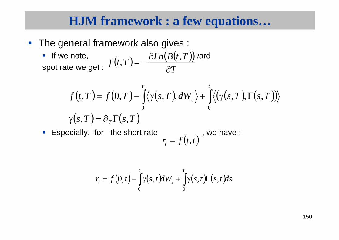
The general framework also gives :If we note, the forward
spot rate we get :
Especially, for the short rate , we have :
T
TtBLnTtf
,,
TsTs
TsTsdWTsTfTtf
T
tt
s
,,
,,,,,,0,00
ttfrt ,
dststsdWtstfrt
s
t
t
00
,,,,0
151
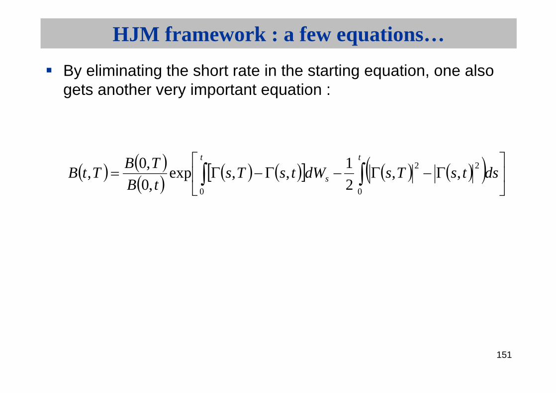
HJM framework : a few equations…
By eliminating the short rate in the starting equation, one alsogets another very important equation :
t t
s dstsTsdWtsTstB
TBTtB
0 0
22,,
2
1,,exp
,0
,0,

152
LGM framework
HJM is a very general framework : for practical implementation and use, need more specifications
LGM (Linear Gaussian Markov model)
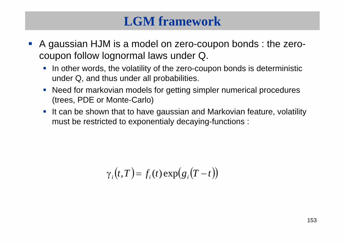
153
LGM framework
A gaussian HJM is a model on zero-coupon bonds : the zero-coupon follow lognormal laws under Q.
In other words, the volatility of the zero-coupon bonds is deterministic under Q, and thus under all probabilities.Need for markovian models for getting simpler numerical procedures (trees, PDE or Monte-Carlo)It can be shown that to have gaussian and Markovian feature, volatility must be restricted to exponentialy decaying-functions :
tTgtfTt iii exp)(,

154
LGM framework
In practice, a good choice for volatilities is :
called mean-reversion parameters, are positive constant
as the instantaneous volatilities, piecewise constant
tTexpt
with
T,t,,T,tT,t
kk
kk
n
1
1
k
k
155
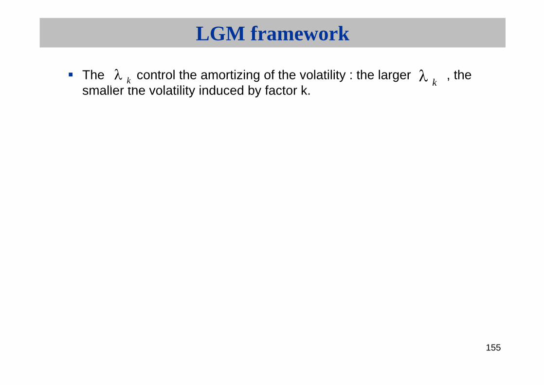
LGM framework
The control the amortizing of the volatility : the larger , the smaller the volatility induced by factor k.
k k
156
LGM-1F model features
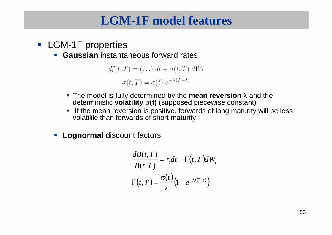
LGM-1F propertiesGaussian instantaneous forward rates
The model is fully determined by the mean reversion and the deterministic volatility (t) (supposed piecewise constant)If the mean reversion is positive, forwards of long maturity will be lessvolatilile than forwards of short maturity.
Lognormal discount factors:
tT
tt
et
Tt
dWTtdtrTtB
TtdB
1,
,),(
),(

157
LGM-1F model features
LGM-1F propertiesGaussian short rate, mean reverting
Forward Libor are shifted lognormal (constant = 1/coverage shift)

158
LGM-1F model features
Reconstruction formula for zero-coupon bonds :the whole dynamics of the curve can be summarized by a single
gaussian state variable :
See previous slide to see that is a gaussian variable.
Remark that :
tfrX tt ,0
tX

159
LGM-1F model features
Then :
Fundamental equation for all numerical methods.This is why we speak of Linear models : zero-coupon bonds canalways be seen as exponential of Linear sum of Gaussian state variables (whatever the number of factors)So zero-coupon rates are Linear sum of these state variables
duee
TtdsestT
t
tutTt
st 1, ,)(
0
22

160
LGM-1F model : vanilla pricing
Analytical formula for vanilla productsStraitghtforward B&S formula for caps & floors as Libor are shiftted Lognormal

161
LGM-1F model : vanilla pricing
For swaptions, let’s define call bond option as a derivative of pay-off :
T is the maturity of the option, is the start date of calibration product
0T
0,,,1
0, where
,,
10
10
i
n
n
iii
cni
TTTTK
TTKBTTBc

162
LGM-1F model : vanilla pricing
The pricing of call and put Bond option is analytical in LGM1F :
)(
)( and ,
)(
:by defined and
,,0
,0
,,,0,,0,,,,
,,,0,,0,,,,
0,
0,
1 0,
0,
0
0
10110
10110
00
0
xB
xBKK
xB
xBc
Kx
TT
ee
TB
TBF
TKFBSputcTBcTKTTPutBO
TKFBScallcTBcTKTTCallBO
TT
TTi
n
i TT
TTi
i
TTTTbsi
ii
n
ii
bsiiinini
n
ii
bsiiinini
ii
i
163
LGM-1F model : vanilla pricing
We use the reconstruction formula for these calculations, especially for the last equations.

164
LGM-1F model : vanilla pricing
Then a payer swaption can be seen as a modified put option :
Payer swaption
Receiver swaption is obtained as a call bond option with sameparameters.
1~
1
1-,1,for
)(,~
,,,,, 1,100
K
Kc
niKc
cTKTTPutBOKTTTswaptionpayer
nn
ii
niniene
165
LGM-1F model : calibration
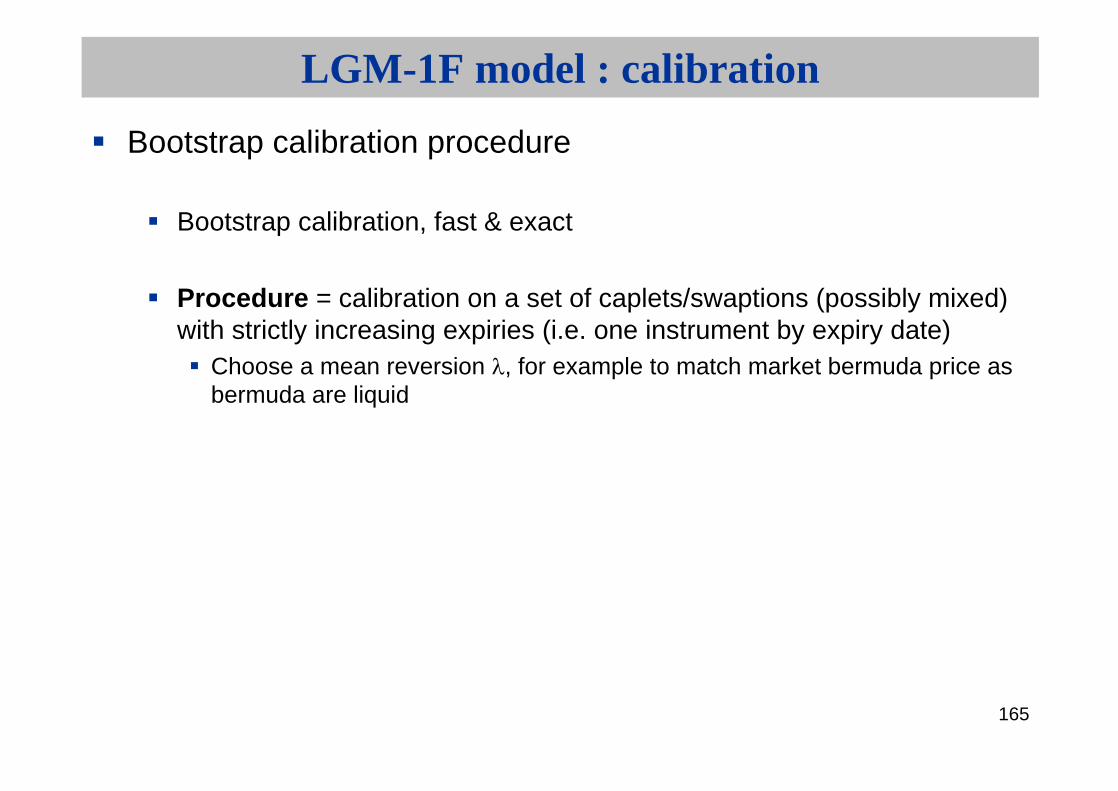
Bootstrap calibration procedure
Bootstrap calibration, fast & exact
Procedure = calibration on a set of caplets/swaptions (possibly mixed) with strictly increasing expiries (i.e. one instrument by expiry date)
Choose a mean reversion , for example to match market bermuda price as bermuda are liquid

166
LGM-1F model : calibration
'T2
1 i2
…..
1T2T 3T ……
'T1
00T
3
i = so called instantaneous volatility between 1iT and iT , used to match the price of option
of maturity iT on underlying of maturity 'iT
instrument (libor for caplet or swap for a swaption ) for option of maturity iT , starts at iT ,
ends at 'iT
167
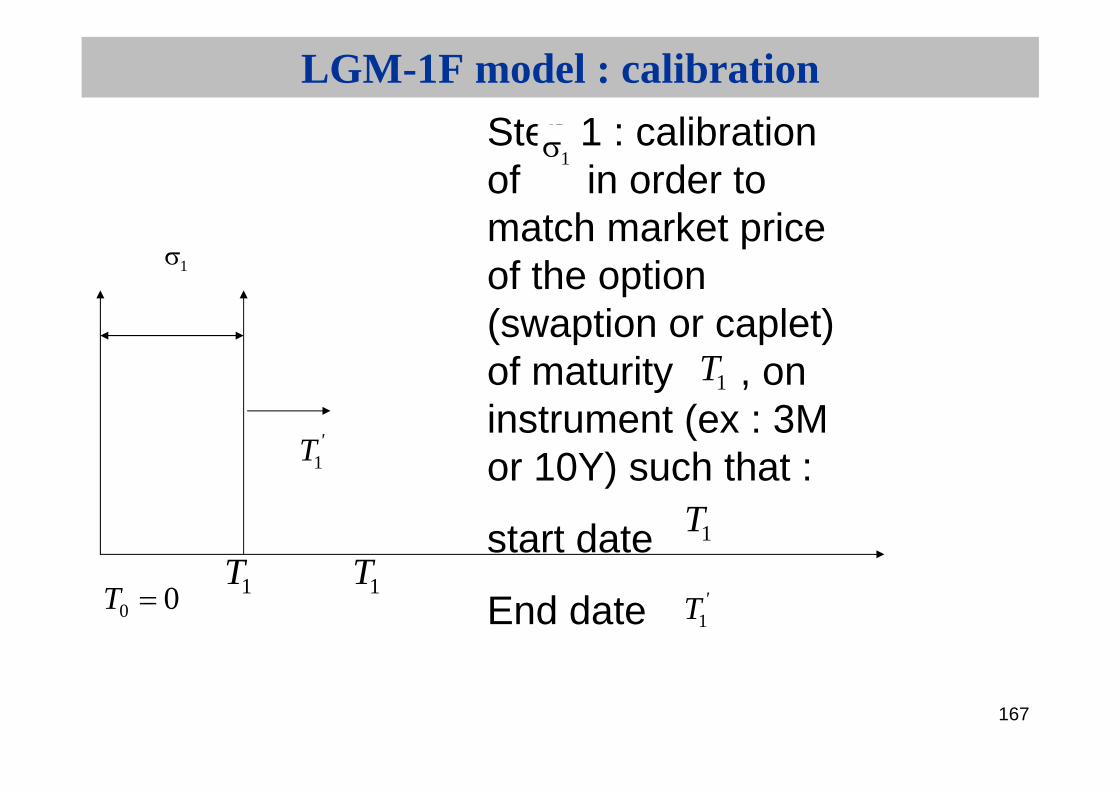
LGM-1F model : calibration
1T
1
1T
'T1
00T
Step 1 : calibration of in order to match market price of the option (swaption or caplet) of maturity , on instrument (ex : 3M or 10Y) such that :
start date
End date
1T
1T
'T1
1

168
LGM-1F model : calibration
2
2
'T2
1T 2T00T
Step 2 : calibration of in order to match market price of the option (swaption or caplet) of maturity ,on instrument such that :
start date
End date
2T
'T2
2T

169
LGM-1F model : calibration
Each instrument provides the variance of the state variable up to its expiry date
The short rate volatility (t), supposed piecewise constant, is then deduced iteratively
170
LGM-1F model calibration
One can iterate the above process to calibrate the mean reversion to a basket of instruments (e.g. to a cap)Depending on the product, we can use a diagonal of swaption (9Y in 1Y, 8Y in 2Y, …1Y in 9Y), for instance for bermudean swaptions ; the strike being the strike of bermudean swaptionsThe set of the calibration is choosen for each exotic product
171
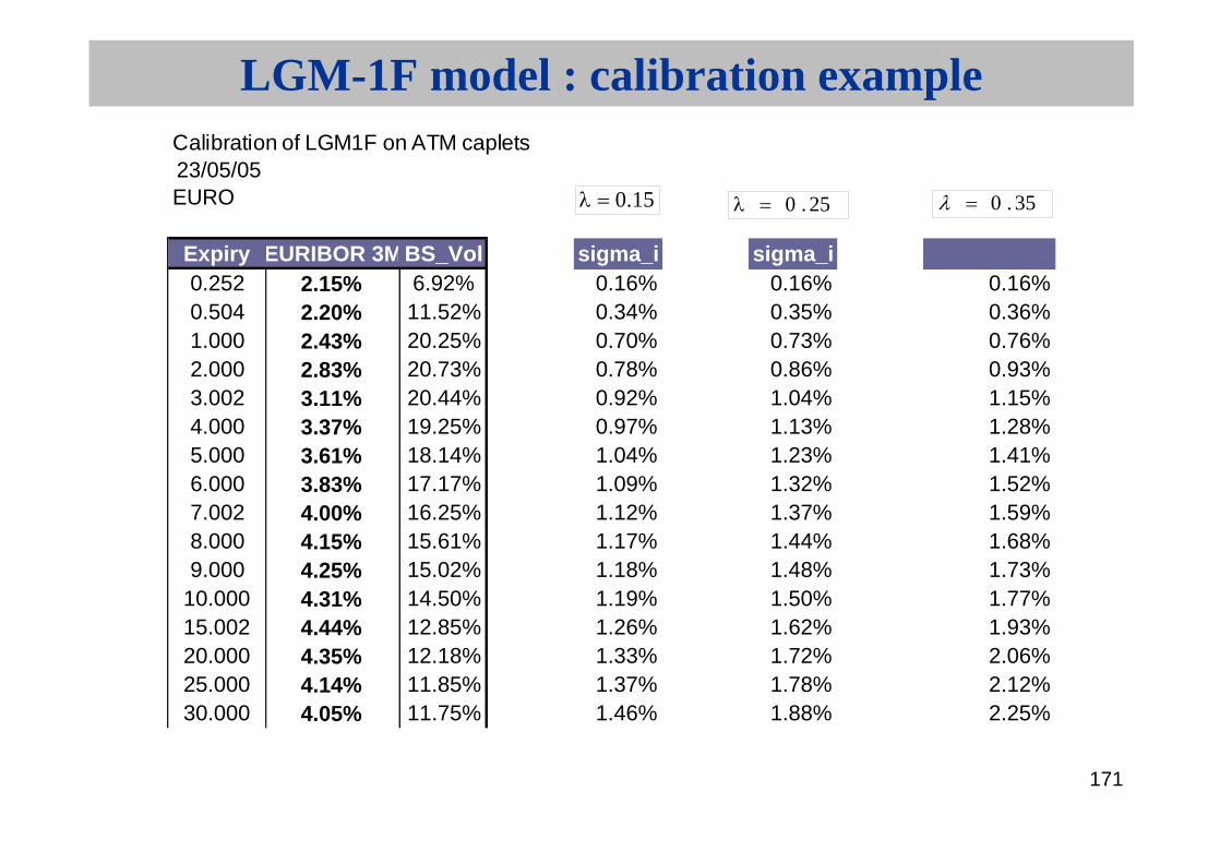
LGM-1F model : calibration exampleCalibration of LGM1F on ATM caplets23/05/05EURO
Expiry EURIBOR 3MBS_Vol sigma_i sigma_i0.252 2.15% 6.92% 0.16% 0.16% 0.16%0.504 2.20% 11.52% 0.34% 0.35% 0.36%1.000 2.43% 20.25% 0.70% 0.73% 0.76%2.000 2.83% 20.73% 0.78% 0.86% 0.93%3.002 3.11% 20.44% 0.92% 1.04% 1.15%4.000 3.37% 19.25% 0.97% 1.13% 1.28%5.000 3.61% 18.14% 1.04% 1.23% 1.41%6.000 3.83% 17.17% 1.09% 1.32% 1.52%7.002 4.00% 16.25% 1.12% 1.37% 1.59%8.000 4.15% 15.61% 1.17% 1.44% 1.68%9.000 4.25% 15.02% 1.18% 1.48% 1.73%
10.000 4.31% 14.50% 1.19% 1.50% 1.77%15.002 4.44% 12.85% 1.26% 1.62% 1.93%20.000 4.35% 12.18% 1.33% 1.72% 2.06%25.000 4.14% 11.85% 1.37% 1.78% 2.12%30.000 4.05% 11.75% 1.46% 1.88% 2.25%
15.0 25.0 35.0

172
LGM-1F model : calibration example
LGM1F and market smiles as of 23/5/2005calibration on ATM 3M caplets
8.00%
13.00%
18.00%
23.00%
28.00%
33.00%
38.00%
43.00%
48.00%
0 0.02 0.04 0.06 0.08 0.1 0.12 0.14
LGM 1Y
LGM 3Y
LGM 5Y
market 1Y
market 3Y
market 5Y
173
LGM-1F model features
Effect of mean reversion on non calibrated instrumentsResult:
If calibration to a short underlying (e.g. a caplet), the price of a long underlying instrument (e.g. a 15Y-term swaption) of same expiry willdecrease as the mean reversion increases
Analogously, if calibration to a long swaption, the price of a caplet of same expiry will increase as lambda increases.

174
LGM-1F model features
Effect of mean reversion on non calibrated instruments (continued)
Example :calibrate to a caplet (expiry = 2Y, term = 1Y), and graph the cumulative vol of B(t,2Y+x) / B(t, 2Y) on [0, 2Y] for various values of mean reversion .calibrate to a long swaption (expiry = 2Y, term = 20Y), and graph the cumulative vol of B(t,2Y+x) / B(t, 2Y) on [0, 2Y] for various values of meanreversion .

175
LGM-1F model features
Calibration on capletCumulative vol of B(t, T+x) / B(t,T)
0.00%
5.00%
10.00%
15.00%
20.00%
0 5 10 15 20
x (years)
lambda = 0.05
lambda = 0.10
Calibration on a 20Y-term swaptionCumulative vol of B(t, T+x) / B(t,T)
0.00%
5.00%
10.00%
15.00%
20.00%
25.00%
0 5 10 15 20
x (years)
lambda = 0.01
lambda = 0.10

176
LGM-1F model features
Effect of mean reversion on forward volatilitiesAssume that we have calibrated to the swaption (Tstart, Tend) (see below). Then the cumulative volatility of the model remains the same for any value of the mean reversion.

177
LGM-1F model features
But because of the exponential shape of the volatility, the forward volatility increases as the mean reversion increases. In the LGM-1F framework, the mean reversion controls the “repartition” of the volatility through time.
Today = T0 Tf Tstart
Tend
mid-curve vol Forward vol

178
LGM-1F model features
Effect of mean reversion on forward volatilities (continued)
Calibration on a 20Y caplet. The graph below represents the instantaneous vol of B(t, 20Y) / B(t, 21Y) for several values of mean reversion.
0.000
0.005
0.010
0.015
0.020
0.025
0.030
1 2 3 4 5 6 7 8 9 10 11 12 13 14 15 16 17 18 19 20
years
vol
( i
--->
i+
1)
lambda = 0.05
lambda = 0.1
lambda = 0.2
lambda = 0.5

179
LGM1F and negative rates
Negatives rates ?
We give the probabilities of 2Y, 5Y, 10Y zero-coupon rates being negative, on the Euro, US, Japan swap market, in march2002.

180
LGM1F and negative rates
Euro 2-year rate
0.0%
0.1%
0.2%
0.3%
0.4%
0.5%
0.6%
0.7%
0.8%
0 4 8 12 16 20Maturity
3.0%
3.5%
4.0%
4.5%
5.0%
5.5%
6.0%
6.5%
7.0%
P(R < 0) under risk-neutral measure Forward ZC Rate (right scale)
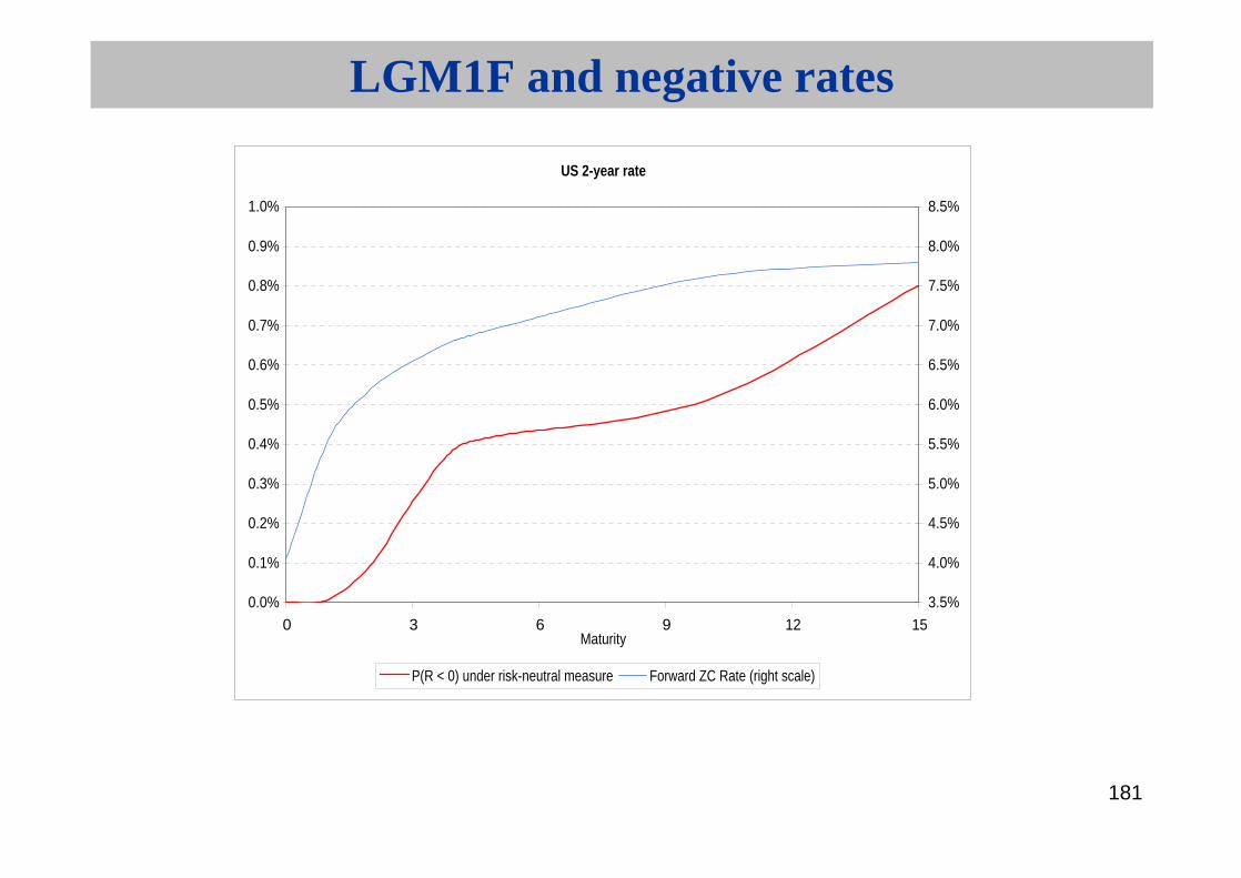
181
LGM1F and negative rates
US 2-year rate
0.0%
0.1%
0.2%
0.3%
0.4%
0.5%
0.6%
0.7%
0.8%
0.9%
1.0%
0 3 6 9 12 15Maturity
3.5%
4.0%
4.5%
5.0%
5.5%
6.0%
6.5%
7.0%
7.5%
8.0%
8.5%
P(R < 0) under risk-neutral measure Forward ZC Rate (right scale)

182
LGM1F and negative rates
Japanese 2-year rate
0.0%
5.0%
10.0%
15.0%
20.0%
25.0%
30.0%
35.0%
0 2 4 6 8 10Maturity
0.0%
0.5%
1.0%
1.5%
2.0%
2.5%
3.0%
3.5%
P(R < 0) under risk-neutral measure Forward ZC Rate (right scale)

183
LGM1F and negative rates
Euro 5-year rate
0.0%
0.1%
0.2%
0.3%
0.4%
0.5%
0.6%
0.7%
0.8%
0 4 8 12 16 20Maturity
3.0%
3.5%
4.0%
4.5%
5.0%
5.5%
6.0%
6.5%
7.0%
P(R < 0) under risk-neutral measure Forward ZC Rate (right scale)

184
LGM1F and negative rates
US 5-year rate
0.0%
0.1%
0.2%
0.3%
0.4%
0.5%
0.6%
0.7%
0.8%
0.9%
1.0%
0 3 6 9 12 15Maturity
3.5%
4.0%
4.5%
5.0%
5.5%
6.0%
6.5%
7.0%
7.5%
8.0%
8.5%
P(R < 0) under risk-neutral measure Forward ZC Rate (right scale)

185
LGM1F and negative rates
Japanese 5-year rate
0.0%
0.5%
1.0%
1.5%
2.0%
2.5%
3.0%
3.5%
4.0%
4.5%
5.0%
0 2 4 6 8 10Maturity
0.0%
0.5%
1.0%
1.5%
2.0%
2.5%
3.0%
3.5%
4.0%
4.5%
5.0%
P(R < 0) under risk-neutral measure Forward ZC Rate (right scale)
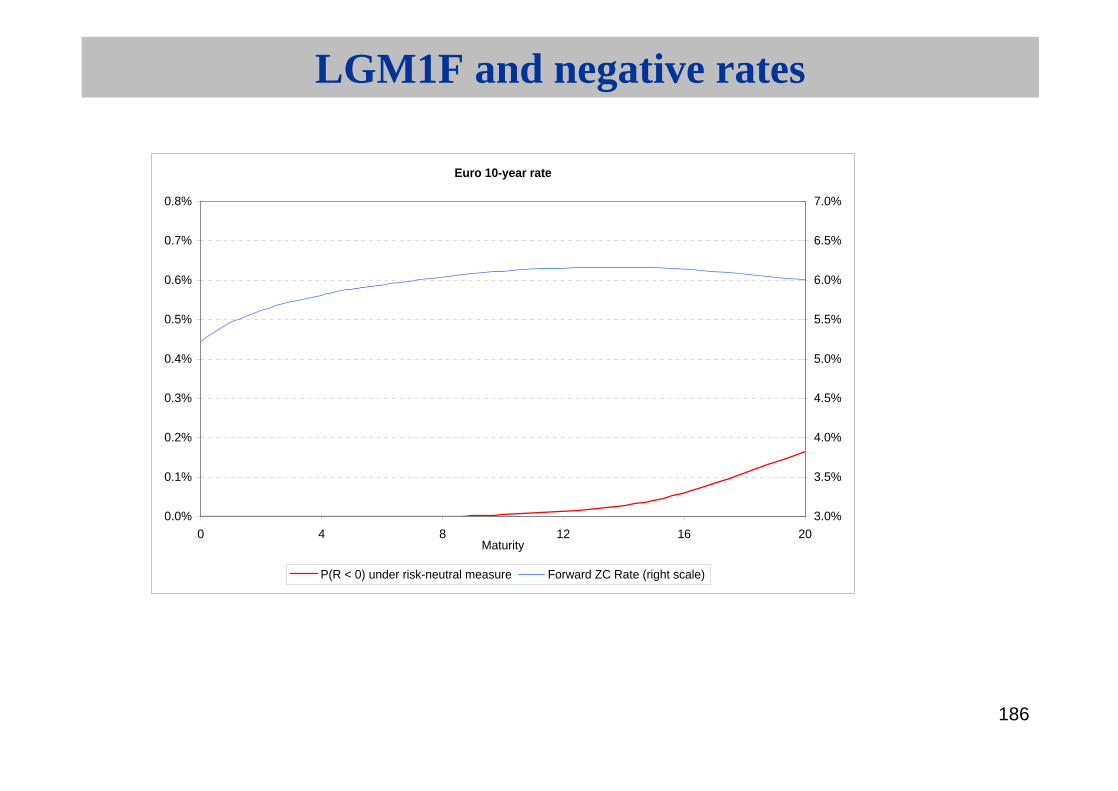
186
LGM1F and negative rates
Euro 10-year rate
0.0%
0.1%
0.2%
0.3%
0.4%
0.5%
0.6%
0.7%
0.8%
0 4 8 12 16 20Maturity
3.0%
3.5%
4.0%
4.5%
5.0%
5.5%
6.0%
6.5%
7.0%
P(R < 0) under risk-neutral measure Forward ZC Rate (right scale)
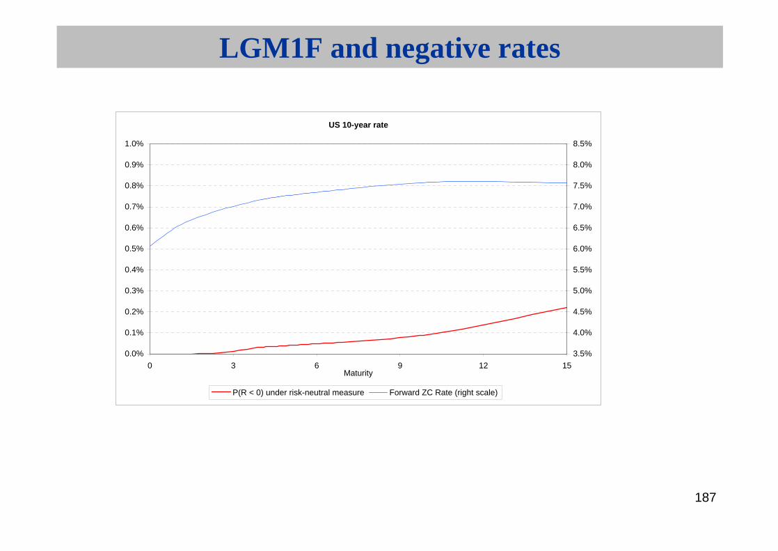
187
LGM1F and negative rates
US 10-year rate
0.0%
0.1%
0.2%
0.3%
0.4%
0.5%
0.6%
0.7%
0.8%
0.9%
1.0%
0 3 6 9 12 15Maturity
3.5%
4.0%
4.5%
5.0%
5.5%
6.0%
6.5%
7.0%
7.5%
8.0%
8.5%
P(R < 0) under risk-neutral measure Forward ZC Rate (right scale)

188
LGM1F and negative rates
Japanese 10-year rate
0.0%
0.5%
1.0%
1.5%
2.0%
2.5%
3.0%
3.5%
4.0%
4.5%
5.0%
0 2 4 6 8 10Maturity
0.0%
0.5%
1.0%
1.5%
2.0%
2.5%
3.0%
3.5%
4.0%
4.5%
5.0%
P(R < 0) under risk-neutral measure Forward ZC Rate (right scale)

189
LGM1F and negative rates
Negative probabilities not very important, except 2Y Yen on short termBe careful nevertheless for very long productsStandard deviation in 2005 similar than in 2002Long term swaps lower in USD, even more in EURShort term swaps lower in EUR, higher in USDYen curve mostly unchanged

190
Digital rate options and applications to exotic swapsComplex Products : digital, steepner, ratchet…Bermuda swaptionsCallablesAppendixes :Standard Deviations vs VolatilitiesSABRCorrelation issuesLGMRisk-Management of exotics

191
Risk-Management for exotics : principles
Vanilla risk ManagementEach underlying (tenor + option maturity : 10Y in 2Y, 10Y in 6Y, 3m in 5Y…) has specific SABR parametersSo some limits for exoticsNevertheless, SABR beta has generally the same value for all underlying
Exotics Risk-managementCalibration of a model for each exotic
Choice of proper vanilla products for calibrationThe vanilla products are for example limits of the exotics in some cases (typicalexample : bermuda swaptions calibrated on diagonal)
Adequation choice of the model for each exotics (number of factors)Some rules (conservative risk-management/pricing) for exotics parameters likemean reversion

192
Risk-Management for exotics : principles
To calculate the greeks (vs interest rates buckets or volatilities)For each exotic,the specific model for is recalibrated on the same set of vanilla products when a market parameters (buckets or volatilities) isbumpedBefore recalibration, new prices of vanilla products are calculated, usingconstant SABR parameters
That’s why so important to have speed and exact calibration method (to avoid excess time calculation) and numerical noiseParameters that are not part of calibration, like mean reversions in a LGM model are kept constant in all the processSABR beta :
The SABR Beta is especially important as it sets the intermediate rule betweenfull normal (beta = 0) and full lognormal model (beta = 1)
SABR Beta, generally common value for all underlying, says how ATM volatilitiesmoves when rates moves
This creates very important consistency feature between Vanilla risk-management and Exotics risk-management

193
■Difference between CPI and DRI■ CPI: consumer price index■ DRI: daily reference index.
■Various indexes traded:
323
1
mm
m
mjCPICPIx
NBD
jCPIDRJ
Index and DRI
INDEX FRENCH XTOB EUR XTOB EUR ITXTOB SP US
BLOOMBERG FRCPXTOB CPTFEMU CPTFIEU ITCPI SPIPC CPURNSA
REUTERS OATINFLATION01 OATEI01 HICPFIX
PUBLISHER INSEE EUROSTAT EUROSTAT ISTAT INDE BLS
01/06/05 01/09/05
July117.20
Inflation : a few definitions

194
INFLATION SWAP CURVES
•The bid/offer spread is between 1 and 8 bp according to the maturity and the market configuration.
•The market size is about 50M €
•European inflation incl. tobacco is less liquid and can not be dealt between two French counterparts ( Evin Law).
Zero coupon curves
1.9
2.1
2.3
2.5
2.7
2.9
3.1
3.3
3.5
1Y 3Y 5Y 7Y 9Y 11Y
13Y
15Y
17Y
19Y
21Y
23Y
25Y
27Y
29Y
FRF EUR EUR ITL ESP

195
INFLATION SWAP CURVESForward curves
1.8
2.0
2.2
2.4
2.6
2.8
3.0
3.2
3.4
3.6
EUR EUR XTOB France Spain Italy
EUR 2.290 2.321 2.270 2.238 2.204 2.218 2.264 2.232 2.248 2.272 2.290 2.312 2.338 2.368 2.393 2.416 2.441 2.469 2.498 2.528 2.553 2.573 2.589 2.626 2.656 2.657 2.680 2.671 2.594
EUR XTOB 2.130 2.159 2.111 2.099 2.107 2.135 2.161 2.122 2.141 2.168 2.186 2.210 2.240 2.275 2.309 2.339 2.366 2.390 2.412 2.429 2.444 2.458 2.473 2.514 2.546 2.547 2.570 2.561 2.484
France 2.036 2.128 2.176 2.152 2.153 2.179 2.206 2.159 2.191 2.256 2.295 2.323 2.342 2.353 2.359 2.371 2.384 2.399 2.415 2.429 2.451 2.471 2.494 2.544 2.575 2.562 2.534 2.526 2.535
Spain 3.330 3.194 3.029 2.947 2.921 2.886 2.812 2.704 2.695 2.709 2.704 2.709 2.720 2.738 2.761 2.782 2.798 2.809 2.815 2.816 2.817 2.823 2.835 2.877 2.903 2.898 2.928 2.937 2.890
Italy 2.410 2.459 2.421 2.389 2.349 2.353 2.387 2.342 2.336 2.330 2.323 2.329 2.347 2.375 2.400 2.420 2.439 2.457 2.475 2.493 2.508 2.517 2.523 2.551 2.557 2.535 2.555 2.563 2.521
1 2 3 4 5 6 7 8 9 10 11 12 13 14 15 16 17 18 19 20 21 22 23 24 25 26 27 28 29
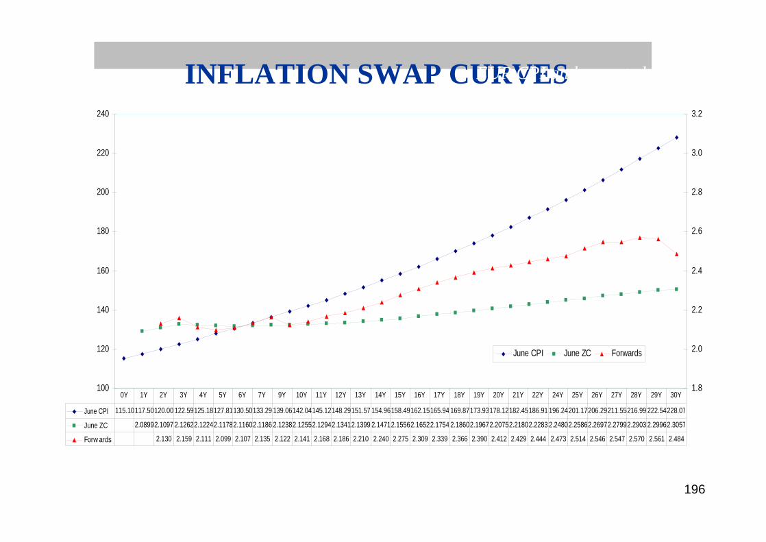
196
INFLATION SWAP CURVESEUR CPI and expectedforwards
100
120
140
160
180
200
220
240
1.8
2.0
2.2
2.4
2.6
2.8
3.0
3.2
June CPI June ZC Forwards
June CPI 115.10117.50120.00 122.59125.18127.81130.50133.29 139.06142.04145.12148.29151.57 154.96158.49162.15165.94 169.87173.93178.12182.45186.91 196.24201.17206.29211.55216.99 222.54228.07
June ZC 2.08992.1097 2.12622.12242.11782.11602.1186 2.12382.12552.12942.13412.1399 2.14712.15562.16522.1754 2.18602.19672.20752.21802.2283 2.24802.25862.26972.27992.2903 2.29962.3057
Forw ards 2.130 2.159 2.111 2.099 2.107 2.135 2.122 2.141 2.168 2.186 2.210 2.240 2.275 2.309 2.339 2.366 2.390 2.412 2.429 2.444 2.473 2.514 2.546 2.547 2.570 2.561 2.484
0Y 1Y 2Y 3Y 4Y 5Y 6Y 7Y 9Y 10Y 11Y 12Y 13Y 14Y 15Y 16Y 17Y 18Y 19Y 20Y 21Y 22Y 24Y 25Y 26Y 27Y 28Y 29Y 30Y
197
Inflation swaps
■ NB:■ There is no calculation basis on the inflation leg. It is an index
performance between two unadjusted dates.■ The calculation basis on the fixed leg is 30/360 on unadjusted dates.■ To make it simple, on the interbank market of European inflation swaps,
the DIR is not interpolated but dealt on m-2 or m-3

198
■ The flows are the following:
against euribor 3M
■For example the fixed rate (real rate) is equal to 1.01% on French inflation ex-tobacco at 10 years.
1;InitialDIR
TDIRMaxmaturityat 0 Rate Fixed*
InitialDIR
iDIR
The « OATi format » swap
Inflation swaps


