33
PRODUCTION AND ESTIMATION CHAPTER # 4
| Date post: | 29-Dec-2015 |
| Category: |
Documents |
| Upload: | emery-watkins |
| View: | 216 times |
| Download: | 0 times |
PRODUCTION AND ESTIMATION
CHAPTER # 4

Introduction
Production is the name given to that transformation of factors into goods.
Production refers to all of the activities involved in the production of goods and services, from borrowing to setting up or expanding production facilities, to hiring workers, purchasing raw materials, running quality control, cost accounting and so on rather than referring merely to the physical transformation of inputs into outputs of goods and services.

Inputs
E.g. land, labour and capital Fixed inputs: The inputs which cannot be
changed readily during the time period under consideration, perhaps at very great expense. E.g. plant and some specialized equipment ( IBM took several years to build a new factory to produce computer chips to go into its own computers).
Variable input: inputs which can be changed on a very short notice e.g, raw material and unskilled labour.
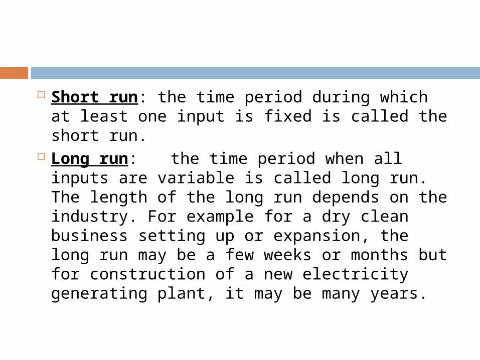
Short run: the time period during which at least one input is fixed is called the short run.
Long run: the time period when all inputs are variable is called long run. The length of the long run depends on the industry. For example for a dry clean business setting up or expansion, the long run may be a few weeks or months but for construction of a new electricity generating plant, it may be many years.

Production Table and Production Function
A production table shows the output resulting from various combinations of factors of production or inputs.
Marginal product is the additional output that will be forthcoming from an additional worker, other inputs remaining constant.
Average product is calculated by dividing total output by the quantity of the input.
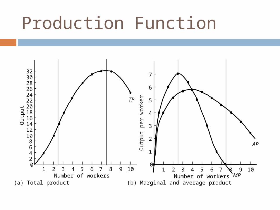
Production function – a curve that describes the relationship between the inputs (factors of production) and outputs.
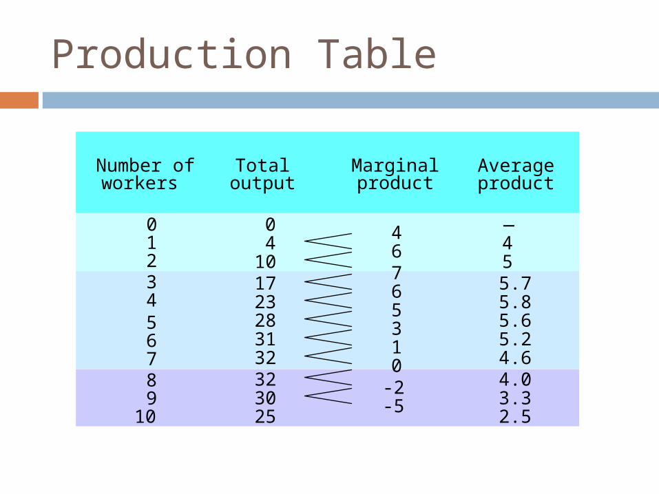
Production Table
Number of workers Total output Marginal
productAverage product
46765310
-2-5
123456789
10
0455.75.85.65.24.64.03.32.5
—4
101723283132323025
0
Out
put
32 30 28 26 24 22 20 18 16 14 12 10 8 6 4 2 0
1 2 3 4 5 6 7 8 9 10Number of workers
TP
Out
put p
er w
orke
r
1 2 3 4 5 6 7 8 9 10Number of workers
7
6
5
4
3
2
1
0
MP(a) Total product (b) Marginal and average product
AP
Production Function
At first MP rises with workers
Initially, By adding more workers the output increases at a greater rate because of specialization.
MP of each worker added is larger than previous worker.
This is because of law of Increasing Marginal Returns.

then, MP falls with more workers
If we keep on increasing number of workers with the same amount of capital, eventually the MP will fall.
MP of next worker will be smaller than MP of previous workers.
This is because of law of decreasing marginal returns

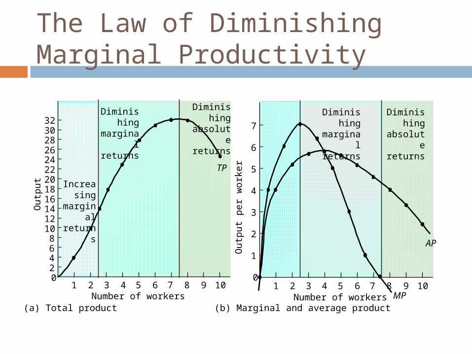
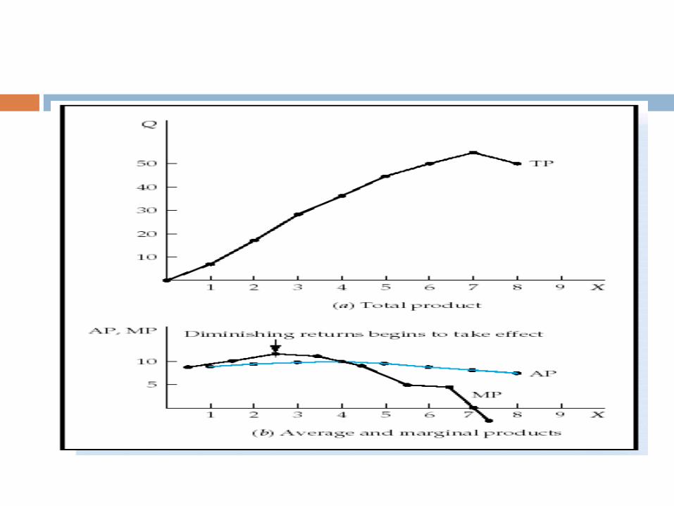
The Law of Diminishing Marginal Productivity Law of diminishing marginal productivity –
As more and more of a variable input is added to an existing fixed input, after some point the additional output one gets from the additional input will fall.

The Law of Diminishing Marginal Productivity
Number of
workers Total
outputMargina
l product
Average product
Increasing marginal returns
Diminishing marginal returns
Diminishing absolute returns
46765310
-2-5
123456789
10
0455.75.85.65.24.64.03.32.5
—4
101723283132323025
0
Out
put
Diminishing marginal returns
Diminishing absolute
returns32 30 28 26 24 22 20 18 16 14 12 10 8 6 4 2 0
1 2 3 4 5 6 7 8 9 10
Increasing marginal
returns
Number of workers
TP
Out
put p
er w
orke
r
1 2 3 4 5 6 7 8 9 10Number of workers
7
6
5
4
3
2
1
0
MP
Diminishing marginal returns
Diminishing absolute
returns
(a) Total product (b) Marginal and average product
AP
The Law of Diminishing Marginal Productivity

The Law of Diminishing Marginal Productivity This law is also called the flower pot law.
• If it did not hold true, the world’s entire food supply could be grown in a single flower pot.
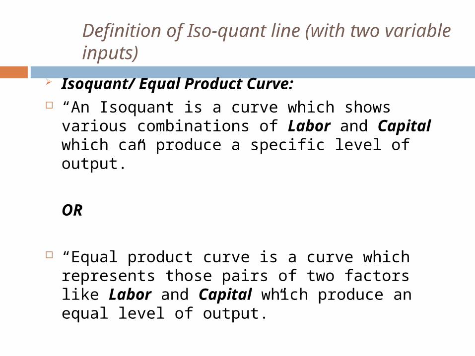
Definition of Iso-quant line (with two variable inputs)
Isoquant/ Equal Product Curve: “An Isoquant is a curve which shows various
combinations of Labor and Capital which can produce a specific level of output.”
OR
“Equal product curve is a curve which
represents those pairs of two factors like Labor and Capital which produce an equal level of output.”

Isoquant line (cont’d):
Here the production depends upon Labor and Capital. Accordingly the production function will be as; Q = f (L, K) CombinationsOf factors
L K Total
output
ABCDE
16 1 500 Meters 12 2 500 Meters 9 3 500 Meters7 4 500 Meters 6 5 500 Meters

Isoquant line (cont’d):
Diagrammatical representation:
1 2 3 4 5
3
6
9
12
15
Y
X
IQ
Labor
Capital

PRINCIPLE OF DIMINISHING MRTS

Marginal Rate of Technical substitution (MRTS) The rate at which the factor can be
substituted at the margin without changing the level of output.
OR It can also be stated like “the loss of
certain units of Factors X which will just be compensated by an additional units of Factor Y at that point”.

Diminishing MRTS
Combinations FactorX(Labor)
FactorY(Capital)
MRTS OutputMeters
A 16 1 ------ 500
B 12 2 4:1 500
C 9 3 3:1 500
D 7 4 2:1 500
E 6 5 1:1 500

ISO-QUANT MAP
Y
X
IQ 1 500m
IQ 3 700m
IQ 2 600m
Labor
0
Capital
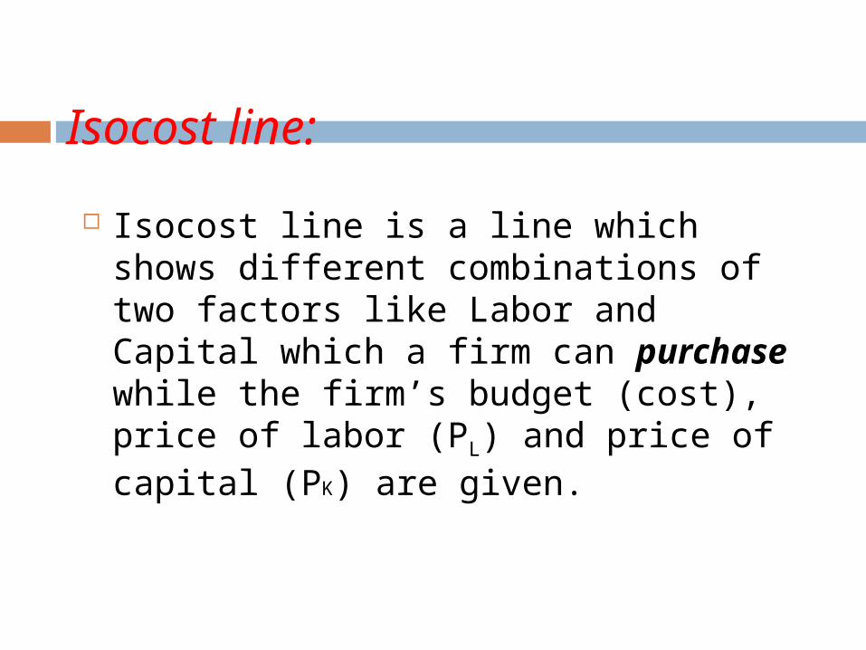
Isocost line:
Isocost line is a line which shows different combinations of two factors like Labor and Capital which a firm can purchase while the firm’s budget (cost), price of labor (PL) and price of capital (PK) are given.

Cont`d
The Iso-cost curves are also called outlay lines, price lines or factor cost lines.
Each price line represents the different combinations of two inputs that a firm can buy for a given sum of money at the given prices of each output.
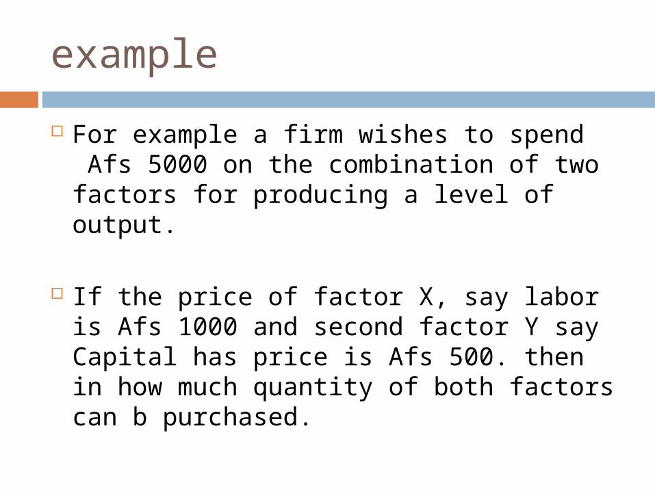
example
For example a firm wishes to spend Afs 5000 on the combination of two factors for producing a level of output.
If the price of factor X, say labor is Afs 1000 and second factor Y say Capital has price is Afs 500. then in how much quantity of both factors can b purchased.
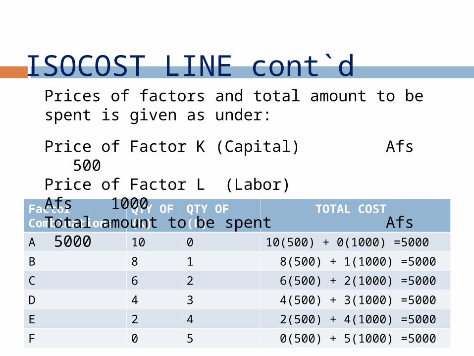
ISOCOST LINE cont`d
Factor Combinations
QTY OF (K)
QTY OF (L)
TOTAL COST
A 10 0 10(500) + 0(1000) =5000
B 8 1 8(500) + 1(1000) =5000
C 6 2 6(500) + 2(1000) =5000
D 4 3 4(500) + 3(1000) =5000
E 2 4 2(500) + 4(1000) =5000
F 0 5 0(500) + 5(1000) =5000
Prices of factors and total amount to be spent is given as under:
Price of Factor K (Capital) Afs 500Price of Factor L (Labor) Afs 1000Total amount to be spent Afs 5000

Graphical presentation Iso Cost line.
Y
X
10
8
6
4
2
0 1 2 3 4 5
A
B
C
D
E
F
Iso Cost line
Factor K
Factor L
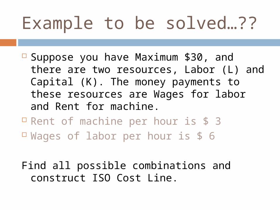
Example to be solved…??
Suppose you have Maximum $30, and there are two resources, Labor (L) and Capital (K). The money payments to these resources are Wages for labor and Rent for machine.
Rent of machine per hour is $ 3 Wages of labor per hour is $ 6
Find all possible combinations and construct ISO Cost Line.

Least Cost Combination for Producer`s Equilibrium.
Least cost combination refers to the combination of factors with which a firm can produce a specific quantity of output at the lowest possible cost.

Cont`d
Least cost combination of factors for any level of output is that where the Isoquant curve is tangent to an Isocost curve.For this we have following assumptions
1 There are only two factors X & Y.2 The prices of factors X & Y are constant.3 The total money to spend is given.
Producer equilibrium can be obtained at the point where:
1 Iso-quant is tangent to the Isocost line or in other words slopes of both curves are the same,
2 Iso-quant must be convex to origin.
Producer Equilibrium

Producer Equilibrium Least cost combination for producer`s
equilibrium. Y
X
R
Capital
Labor
0
C
S
T
A B
A
B
C
a
f
Equilibrium point
IQ

Thanks


