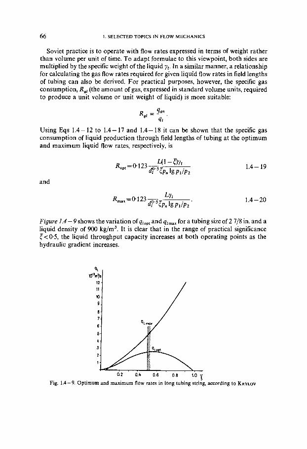
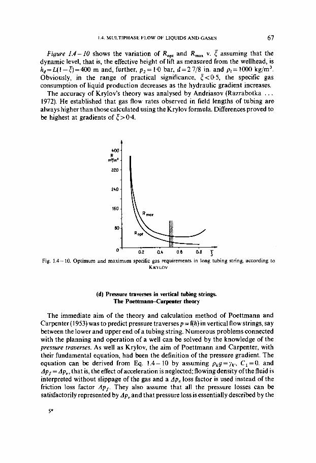
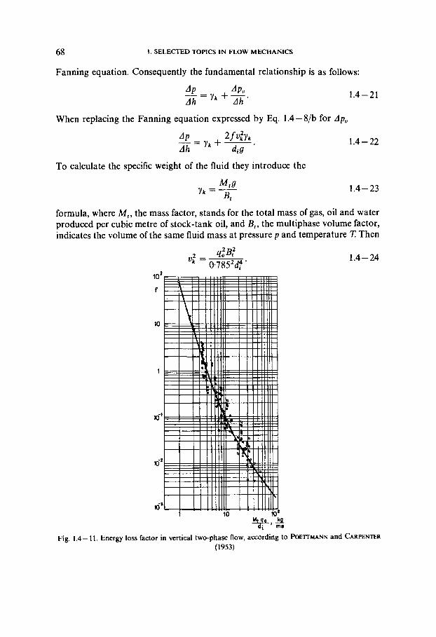
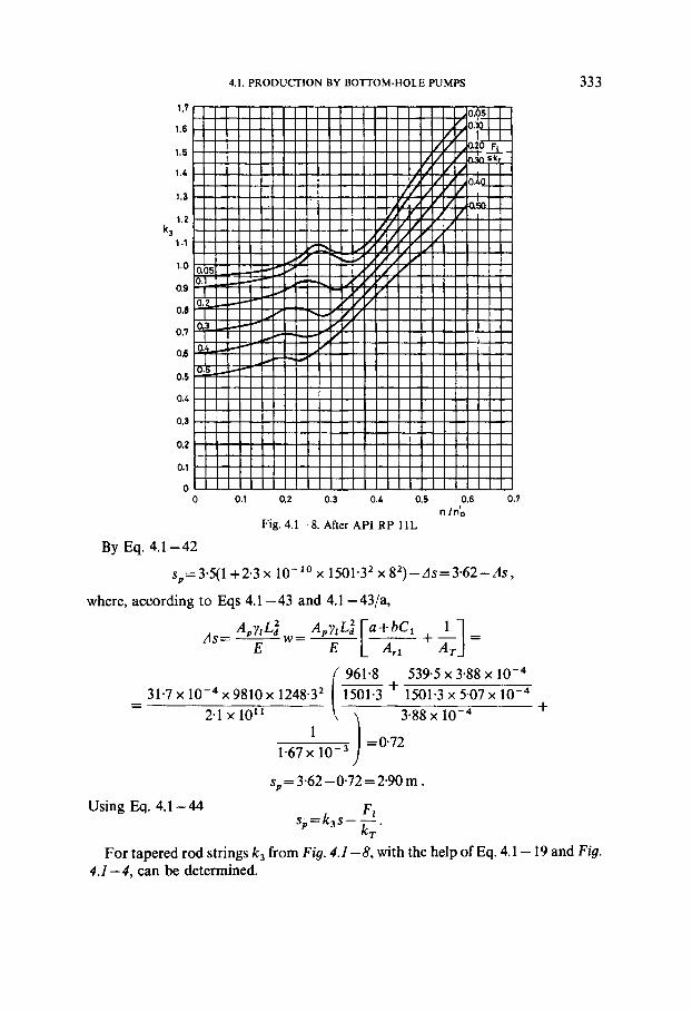
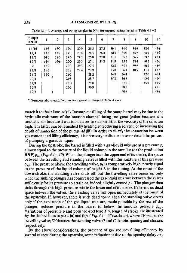
Developments in Petroleum Science, 18 A PRODUCTION AND TRANSPORT OF OIL AND GAS Second completely revised edition PART A Flow mechanics and production by A. P. SZILAS Professor of Petroleum Engineering Petroleum Engineering Department Mi,skolc Technical Univer.sity,/or Heavy Industries, Hungary ELSEVIER Amsterdam-Oxford-New York-Tokyo 1985
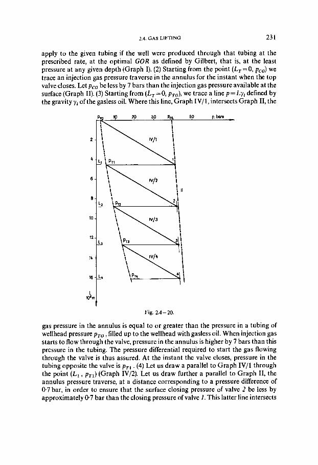
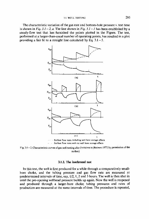
Transcript
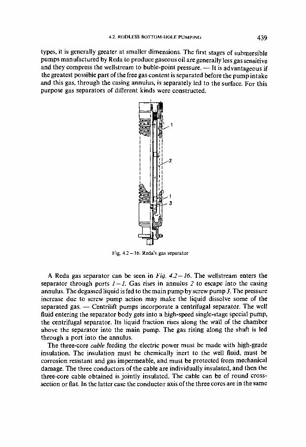
Developments in Petroleum Science, 18 A
PRODUCTION AND TRANSPORT OF OIL AND GAS Second completely revised edition
PART A Flow mechanics and production
by A. P. SZILAS Professor of Petroleum Engineering Petroleum Engineering Department Mi,skolc Technical Univer.sity,/or Heavy Industries, Hungary
ELSEVIER
Amsterdam-Oxford-New York-Tokyo 1985
Joint edit~on published by
Elsevier Science Publishers, Amsterdam, The Netherlands and Akadkmiai Kiad6, the Publishing House of the Hungarian Academy of Sciences, Budapest. Hungary
First English edition 1975 Translated by B. Balkay
Second revised and enlarged edition 1985 Translated by B. Balkay and A. Kiss
The distribution of this book is being handled by the following publishers
for the U.S.A. and Canada
Elsevier Science Publishing Co., Inc. 52'Vanderbilt Avenue, New York, New York 10017, U.S.A.
for the East European Countries, Korean People's Republic, Cuba. People's Republic of Vietnam and Mongolia
Kultura Hungarian Foreign Trading Co., P.O.Box 149, H-1389 Budapest, Hungary
for all remaining areas Elsevier Science Publishers Molenwerf 1. P.O.Box 21 1, 1000 AE Amsterdam, The Netherlands
Library of Congress Cat.logiog Data
Szilas, A. PHI. Production and transport of oil and gas.
(Developments in petroleum science; 18A-) Translation of KGolaj i s foldgbtermeles. 1. Petroleum engineering. 2. Petroleum-Pipe lines.
3. Gas, Natural-Pipe lines. I. Title. 11. Series. TN870.S9413 1984 62T.338 84-13527 ISBN W 9 9 5 9 8 - 6 (V. 1) ISBN w 9 9 5 6 4 - 1 (Series)
0 Akadhniai Kiado, Budapest 1985
Printed in Hungary
Preface
TO THE SECOND EDITION
The material of the first edition is considerably revised in this second two-volume edition. The changes can be ranged in three groups: I wished to take into account the latest developments in the world oil industry and incorporate the latest research of my Institute; I have modified some chapters to make it easier for readers to cope with the material; the field of trade, as indicated in the title is more consciously determined, and therefore the content and length of some chapters - primarily in the second volume - are changed.
It would be a great pleasure if through this work I could contribute to the acceptance of the "production and transport of oil and gas" as a specific field of science and technology of oil and gas "mining".
I should like to express my sincere gratitude to my co-workers who participated in the preparation of this work. First of all, I wish to emphasize the assistance of Mr. Gabor Takacs and his always helpful contributions. The high quality work on the figures was done by Mrs. ~ v a Szota. Ms. Piroska Polyinszky, the editor, took upon herselftheexacting task ofproof-reading the text. Last but not least I wish to express my special thanks to my wife, Mrs. Elisabeth Szilas. She showed patience and goodwill towards my having spent years on the rewriting of my book and she was my untiring helper in preparing the manuscript.
The Author
Preface TO THE FIRST EDITION
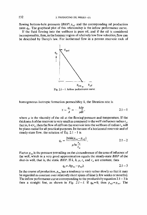
Oil and gas production in the broad sense of the word can be subdivided into three more or less separate fields of science and technology, notably (1) production processes in the reservoir (reservoir engineering), (2) production of oil and gas from wells, and finally (3) surface gathering, separation and transportation. The present book deals with the second and the last of the three topics.
Chapter 1 reviews those calculations concerning flow in pipelines a knowledge of which is essential to the understanding and designing of single-phase and multi- phase flow in wells and in surface flow lines.
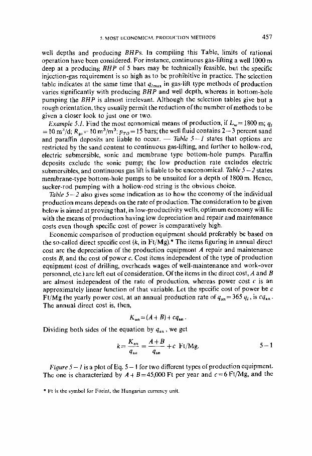
In compiling Chapters 2-5 , which deal with oil and gas wells and in the treatment of those subjects, I have followed the principle that the main task of the production engineer is to ensure the production of that amount of liquid and/or gas prescribed for each well in the field's production plan, at the lowest feasible cost of production. The technical aim outlined above can often be attained by several different methods of production, with several types of production equipment and, within a given type, with various design and size of equipment; in fact, using a given type of equipment, several methods of operation are possible. Of the technically feasible solutions, there will be one that will be the most economical; this, of course, will be the one chosen.
I have attempted to cover the various subjects as fully as possible, but have nevertheless by-passed certain topics which are treated in other books, such as the dynamometry of sucker rod pumps and gas metering. A discussion of these topics in sufficient depth would have required too much space.
Chapter 6 deals with the main items of surface equipment used in oil and gas fields. In this case, I have also aimed at conveying a body of information setting out the choice of the technically and economically optimal equipment.
Equipment is not discussed in Chapters 7 and 8 which treat the flow of oil and gas in pipelines and pipeline systems. The reason for this is that comparatively short pipelines are encountered within the oil or gas field proper, and the relevant production equipment is discussed in Chapter 6; on the other hand, it seemed reasonable to emphasize the design conception which regards the series-connected hydraulic elements of wells, on-lease equipment and pipelines as a connected hydraulic system with an overall optimum that can be and must be determined. It
12 PREFACE
should be emphasized, however, that this method of designing also requires a knowledge of rheology.
Naturally, in the treatment of each subject I have attempted to expose not only the "hows" but also the "whys" and "wherefores" of the solutions outlined. It is a regrettable phenomenon, and one which I have often found during my own production experience and in my work at the University, that the logical consistency as well as the economy of the solution adopted will tend to suffer because the design or production engineer is just following "cookbook rules" without understanding what he is actually trying to do. An understanding of the subject is a necessary critical foundation, and this is a prime reason of textbooks and handbooks.
In denoting physical quantities and in choosing physical units I have followed the SI nomenclature. In choosing the various suffixes to the symbols used in this book, the wide range of the subjects covered has necessitated some slight deviations from the principle of "one concept - one symbol". I sincerely hope that such compromises, adopted for the sake of simplicity, will not create any difficulties for the reader.
In compiling the present volume and in its preparation for publication I have been assisted by many of my co-workers at the Petroleum Engineering Department of the Miskolc Technical University of Heavy Industries. I am deeply grateful for their cooperation, without which the present book, a compendium of three decades' production and teaching experience, could hardly have been realized. Among them I wish to give special credit to Ferenc Patsch, Jr., who played a substantial part in the writing of Chapter 8, to Gabor Takhcs and Tibor Thth, both of whom gave a great deal of help in the calculation and correction of the numerical examples in Chapters 1-7, and to Mrs. E. Szota for her painstaking work concerning the figures.
The Author
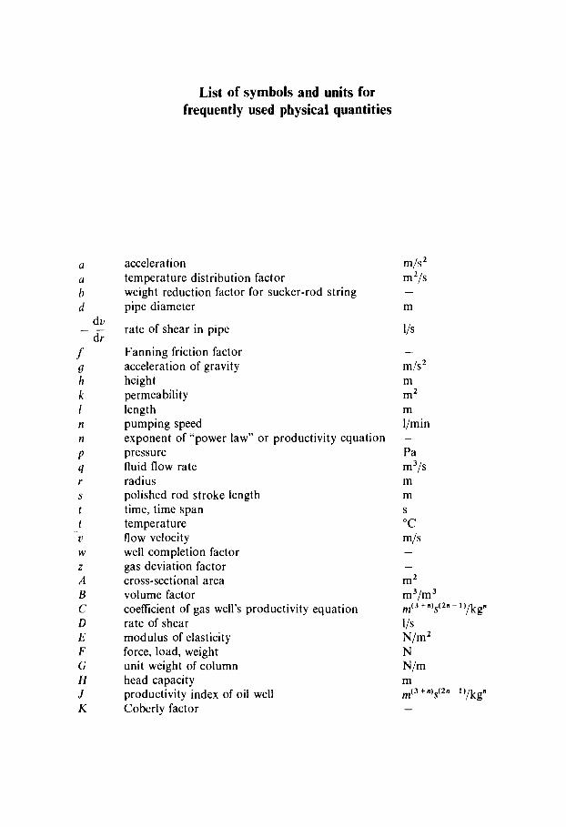
List of symbols and units for frequently used physical quantities
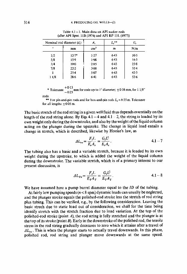
acceleration temperature distribution factor weight reduction factor for sucker-rod string pipe diameter
rate of shear in pipe
Fanning friction factor acceleration of gravity height permeability length pumping speed exponent of "power law" or productivity equation pressure fluid flow rate radius polished rod stroke length time, time span temperature flow velocity well completion factor gas deviation factor cross-sectional area volume factor coefficient of gas well's productivity equation rate of shear modulus of elasticity force, load, weight unit weight of column head capacity productivity index of oil well Coberly factor
LJST OF SYMBOLS
Sub- script
length, depth torque molar mass mass factor dimensionless number power universal molar gas constant volumetric ratio of fluids dimensionless slippage velocity temperature volume work, energy angle of inclination, angular displacement specific weight cross-sectional fraction efficiency dynamic factor for sucker-rod pumping ratio of specific heats Weisbach friction factor thermal conductivity factor dynamic viscosity kinematic viscosity dimensionless pressure gradient density normal stress, strength geothermal gradient shear stress angular velocity, cycle frequency
allowable stress bubble point pressure critical pressure diameter of valve port fluid flow rate pressure drop to friction flowing bottom-hole pressure of well gas rate inside cross-sectional area of pipe
LIST OF SYMBOLS 15
k m m max min n a a opt P P r S
S
mixture UP
motor Pm mass urn maximal Fmax minimal Fmin
standard state P" outside do oil 40 optimal dopt plunger A , Pump rod
LP A,
polished rod Fs superficial (only for symbols v, first letter) us,
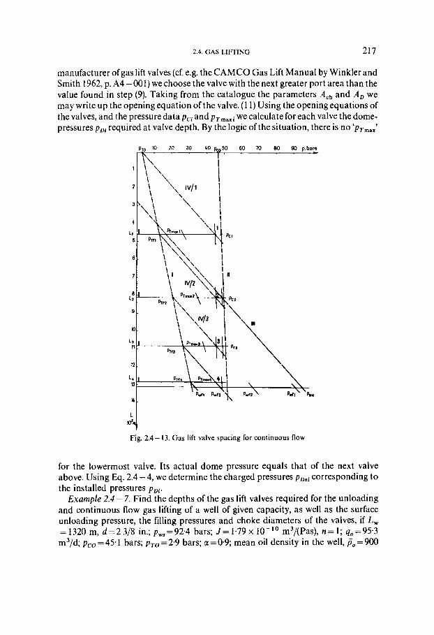
slippage (only for symbol v,, second subscript) multiphase Bt well Lw water q w casing PC valve dome TD depth PL tubing PT surface, wellhead PTO
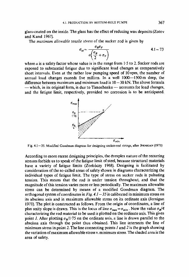
OTHER SYMBOLS
mixture flow velocity motor power mass flow velocity maximum load minimum load standard pressure outside diameter of pipe oil flow rate optimal pipe diameter plunger's cross-sectional area pump setting depth cross-sectional area of rod polished rod load
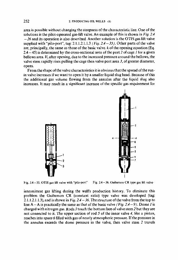
superficial gas velocity
gas slippage velocity multiphase volume factor well depth water rate casing pressure valve dome temperature pressure at depth L tubing pressure surface tubing pressure
A difference (before symbol) A p pressure difference - average (above symbol) P average pressure
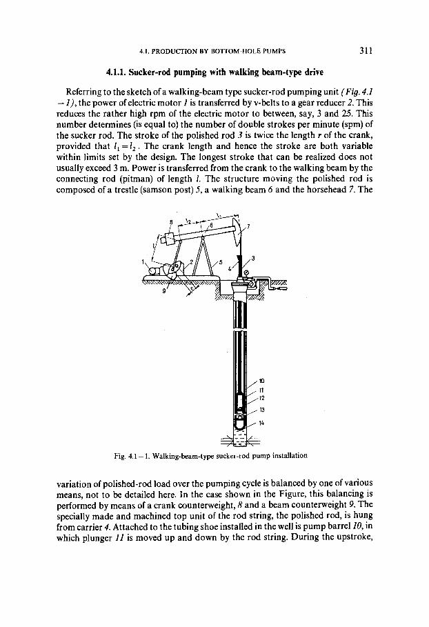
CHAPTER 1
SELECTED TOPICS IN FLOW MECHANICS
1.1. Fundamentals of flow in pipes
Pressure drop due to friction of an incompressible liquid flowing in a horizontal pipe is given by the Weisbach equation:
v21p A p f = I-,
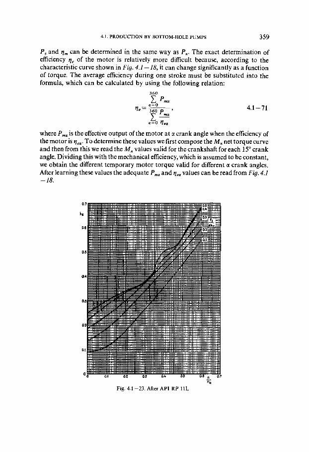
2di
where v = q/A. If the Reynolds number
is less than about 2000-2300, then flow is laminar, and its friction factor I is, after Hagen and Poiseuille,
For turbulent flow in a smooth pipe, for NRe < lo5, the Blasius formula gives a fair approximation:
Likewise for a smooth pipe and for Nu,> lo5, the explicit Nikuradse formula is satisfactory:
A.=0-0032+0.221~R;0'~~~. 1.1 -5
The Prandtl-Karman formula
is valid over the entire turbulent region but its implicit form makes it difficult to manipulate. In rough pipes, for the transition zone between the curve defined by Eq.
18 1. SELECTED TOPICS 1N FLOW MECHANICS
1.1 - 6 and the so-called boundary curve (cf. Eq. 1.1 - 12) the Colebrook formula gives
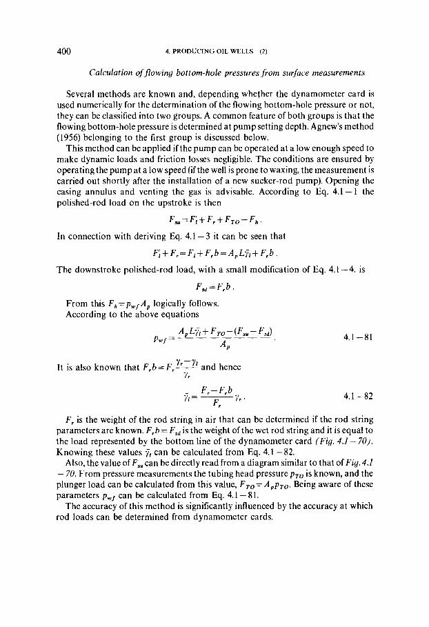
Also for rough pipes, but for the zone beyond the boundary curve, Prandtl and Khrman give the relationship
Although Eqs 1.1 - 7 and 1.1 - 8 provide results sufficiently accurate for any practical purpose, other formulae are often used to determine the pressure drop of turbulent flow in rough pipes, in order to avoid the cumbersome implicit equations. Explicit formulae can be derived from the following consideration.
If we have an idea of the relative roughness to be expected, then we can characterize the relationship A v. NRe by a formula which differs from Eq. 1.1 -6 only in its constants. Consider e.g. the formula of this type of Drew and Genereaux (Gyulay 1942):
Short sections of the graph of this function can be approximated fairly well by an exponential function
A=aN,;b, 1.1 - 10
where a and b are constants characteristic of the actual value of relative roughness and of the NRe range involved. The drawback of formulae of type 1.1 - 10 is that they do not provide a satisfactory accuracy beyond a NRe range broader than just two orders of magnitude. A relationship that is somewhat more complicated but provides a fair approximation over a broader N,, range is the Supino formula
where A,, is the friction factor of smooth pipe, to be calculated using Eq. 1.1 -4 or 1.1 - 5. The graphs of Eqs 1.1 - 3 and from 1.1 - 6 to f . l - 8 are illustrated in the Moody diagram shown as Fig. 1.1 - 1. The dashed curve in the diagram is the boundary curve that separates the transition zone from the region of full turbulence. In the transition zone 1 depends both on the relative roughness k/di and on NRe ,
Fig. 1.1 - 1 . Friction factor in pipes, according to Moody
whereas in the region of full turbulence it is a function of k/di alone. The equation of the boundary curve is
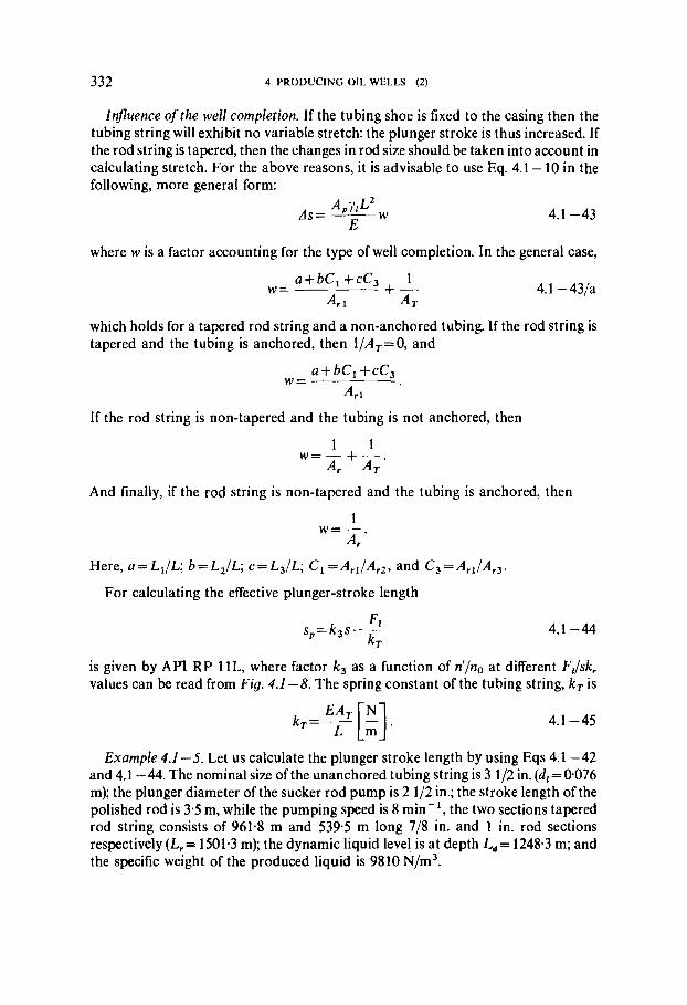
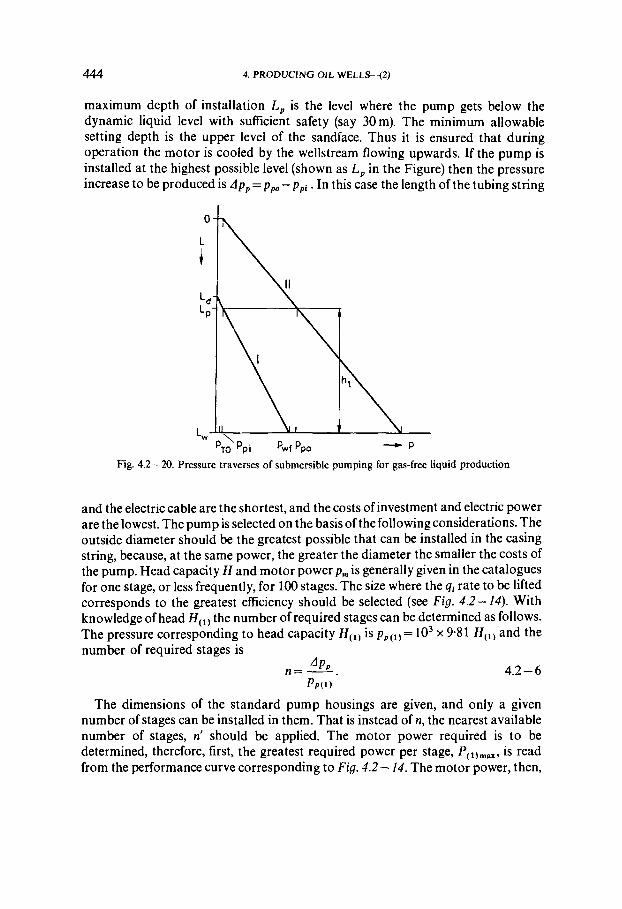
Example 1.1- I. Let us find the friction pressure drop of oil flowing in a horizontal pipeline I = 25 km long, if di =0.300 m, q = 270 m3/h. At the temperature and pressure prevailing in the fluid, v=2.5 cSt and p=850 kg/m3. The pipeline is made of seamless steel pipe, for which k/di=0.00017. Converting the data of the problem to SI units, we have 1 = 25,000 m, di = 0.3 m, q = 0.075 m3/s, v = 2-5 x m2/s, p=850 kg/m3, k/di=0.00017. Flow velocity is
and
2*
20 I . SELECTED TOPICS IN FLOW MECHANICS
Flow is turbulent because 1.27 x 10' is greater than the critical Reynolds number, N,, , = 2300. The Moody diagram (F ig . 1.1 - I ) reveals that for k/di=0.00017, flow is in the transition zone where Eq. 1 . 1 - 7 holds. It enables us to read off directly that, for the case in hand, A=0.018. If a more accurate value is required (which is, however, usually rendered superfluous by the difficulty of accurately determining relative roughness), the value of 1 thus read off the diagram may be put into the right-hand side of Eq. 1.1 -7 and the definitive value of 1 can be found using that equation. The procedure is rather insensitive to the error of reading off the diagram. In the case in hand,
and hence,
Let us calculate the friction factor also from Eq. 1 . 1 - 1 1 , using a A,, furnished by Eq. 1.1-5:
Using in further computation the value 1=0.018 we get by Eq. 1 . 1 - 1 for the flowing pressure drop
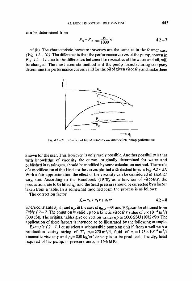
The pressure drop of flow in spaces of annular section can be determined as follows. In Eq. 1 . 1 - 1 , substitute di by the equivalent pipe diameter, d,. In a general way,
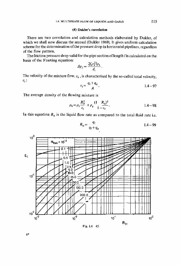
wetted cross section d,=4 x
wetted circumference '
For an annular space, then,
where d l is the ID of the outer pipe and d 2 is the OD of the inner pipe; Eq. 1 . 1 - 1 thus modifies to
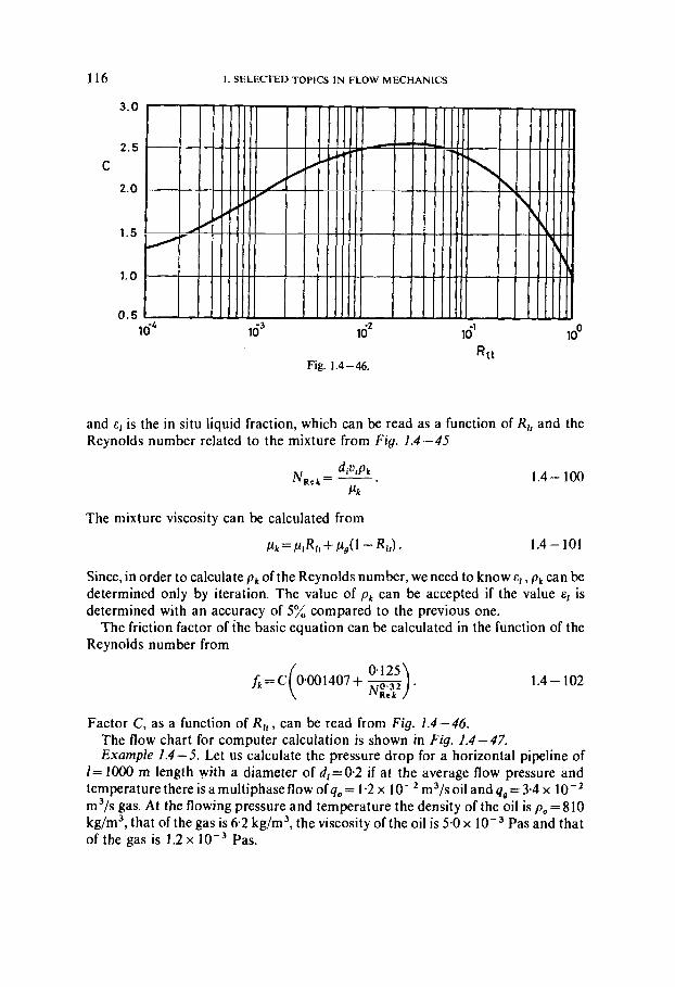
1 .1 . FUNDAMENTALS OF FLOW IN PIPES
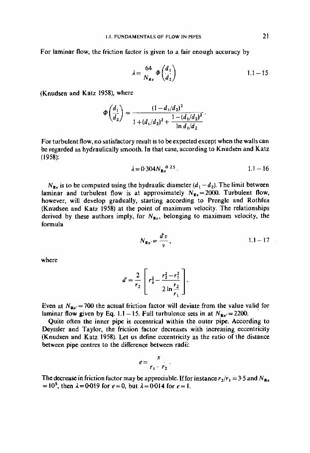
For laminar flow, the friction factor is given to a fair enough accuracy by
(Knudsen and Katz 1958), where
For turbulent flow, no satisfactory result is to be expected except when the walls can be regarded as hydraulically smooth. In that case, according to Knudsen and Katz (1 958):
3, = 0 . 3 0 4 ~ , - , 0 ' ~ ~ . 1.1 - 16
NRe is to be computed using the hydraulic diameter (dl -d2). The limit between laminar and turbulent flow is at approximately N R , = 2 0 0 0 . Turbulent flow, however, will develop gradually, starting according to Prengle and Rothfus (Knudsen and Katz 1958) at the point of maximum velocity. The relationships derived by these authors imply, for N, , , belonging to maximum velocity, the formula
where
Even at N R e , = 7 0 0 the actual friction factor will deviate from the value valid for laminar flow given by Eq. 1.1 - 15. Full turbulence sets in at N,,. = 2200.
Quite often the inner pipe is eccentrical within the outer pipe. According to Deyssler and Taylor, the friction factor decreases with increasing eccentricity (Knudsen and Katz 1958). Let us define eccentricity as the ratio of the distance between pipe centres to the difference between radii:
The decrease in friction factor may be appreciable. If for instance r2 / r l = 3.5 and N R e =lo5, then I=0.019 for e=0, but E.=0.014 for e=1.
I . SELECTED TOPICS IN FLOW MECHANlCS
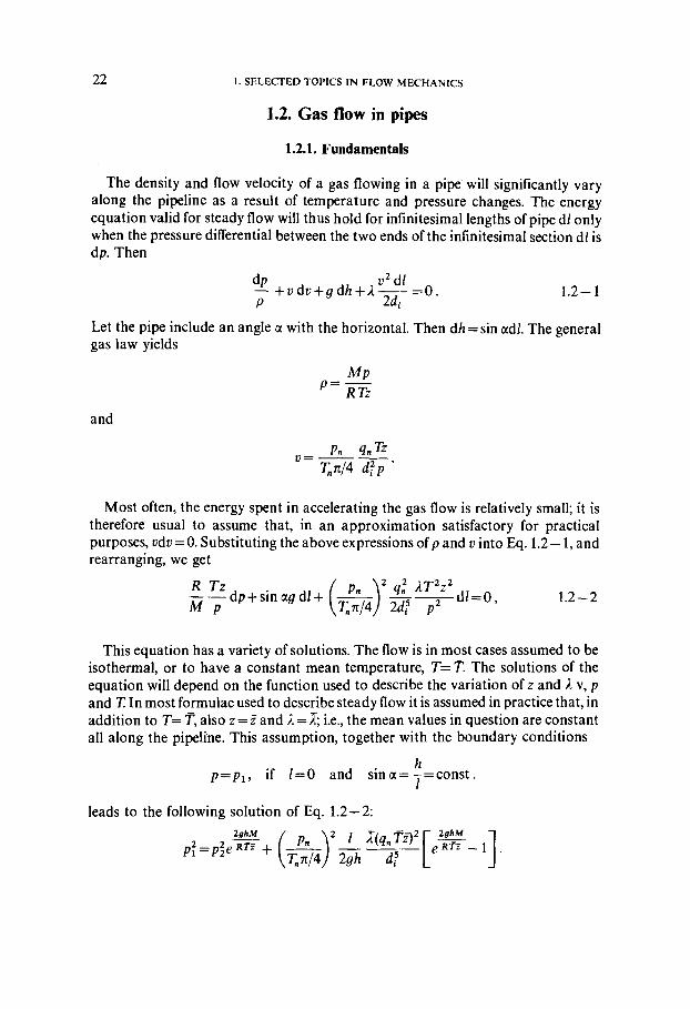
1.2. Gas flow in pipes
1.2.1. Fundamentals
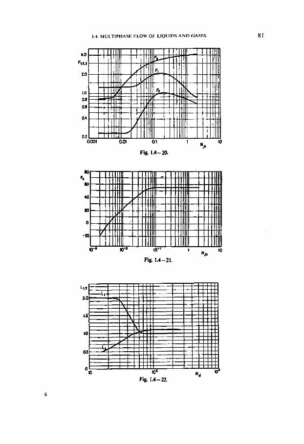
The density and flow velocity of a gas flowing in a pipe will significantly vary along the pipeline as a result of temperature and pressure changes. The energy equation valid for steady flow will thus hold for infinitesimal lengths of pipe dl only when the pressure differential between the two ends of the infinitesimal section dl is dp. Then
Let the pipe include an angle a with the horizontal. Then dh = sin adl. The general gas law yields
and
Most often, the energy spent in accelerating the gas flow is relatively smaI1; it is therefore usual to assume that, in an approximation satisfactory for practical purposes, vdu = 0. Substituting the above expressions of p and v into Eq. 1.2 - 1, and rearranging, we get
This equation has a variety of solutions. The flow is in most cases assumed to be isothermal, or to have a constant mean temperature, T= T. The solutions of the equation will depend on the function used to describe the variation of z and A v, p and 7: In most formulae used to describe steady flow it is assumed in practice that, in addition to T= T, also z = Z and A = 2 i.e., the mean values in question are constant all along the pipeline. This assumption, together with the boundary conditions
h p=p, , if 1=0 and sina=-=const. 1
leads to the following solution of Eq. 1.2-2:
1.2. GAS FLOW IN PIPES
R is 8315; let g=9.8067; then
and hence,
X is expressed in a variety of ways. One of the most widely used formulae was written up by Weymouth:
It gives rather inaccurate results in most cases. Substituting this I for Xin 1.2 -4 we get
In a gas pipeline laid over terrain of gentle relief, the elevation difference h between the two ends of the pipeline can be neglected; Eq. 1.2-2 then yields for the horizontal pipeline, assuming, as in Eq. 1.2 - 4, T= T, z = 2, I = X and 1 = 0 if p = p , :
Substituting R=8315 and the numerical value of n/4, we get
Introducing the value of I given by Weymouth's Eq. 1.2-5 we arrive at the widely used formula
Solving for gas flow rate, we get
Example 1.2 - I . Using Eq. 1.2 - 9 let us find the gas flow rate in a horizontal pipeline if T, = 288-2 K, p, = 1.013 bars, d; =0.1 m, p , = 44.1 bars, p2 = 2.9 bars, T
24 I . SELECTED TOPICS I N FLOW MECHANICS
= 275 K, M = 18.82 kdkmole, 1 = 15 kms. In order to find i; let us first calculate by Eq. 1.2 - 26 an approximate mean pressure p in the pipeline:
(2.9 x 10⁵)~ I =29-5 x 10' Pa. 44.1 x 10⁵+2.9x lo5
According to Diagram 8-1 - 1 p, = 46.7 bars, T, = 207 K, and the reduced parameters p, = 0-63 and T, = I .33 (cf. Eqs 8.1 - 3 and 8.1 - 4). Figure 8.1 - 2 yields Z=0.90. The gas flow rate sought,
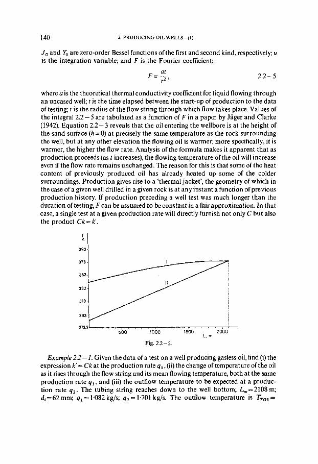
Example 1.2-2. Using Eq. 1.2-6, find the input pressure in the pipeline of the foregoing Example provided the output end of the pipeline is situated higher by h= 150 m than its input end.
In Eq. 1.2 - 3,
and hence
Consequently,
p , = 4.44 M Pa = 44.4 bars .
In the foregoing Example we have had p , =44.1 bars. An input pressure higher by 0 3 bar is thus required to overcome the elevation difference of 150 m if the gas flow rate of 2.383 m3/s is to be maintained.
Equation 1.2-7 becomes a more accurate tool of computation if il is taken from Eq. 1 . 1 - 10 rather than from the Weymouth formula. The Reynolds number figuring in Eq. 1 . 1 - 10 is
where
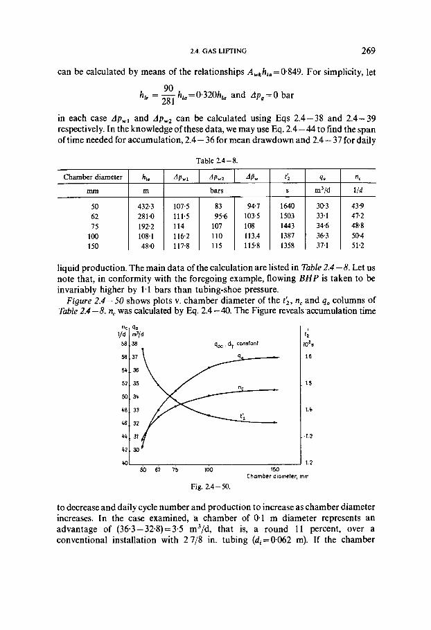
1.2. GAS FLOW IN PIPES
and-the general gas law yields
- M p p q iT P = and q=+.
PZn T,
Substituting the expressions for v, P and q into the fundamental equation and assuming that zn= 1 in a fair approximation, we get
Re- 1 p,qnM N
7c diT , j i - R 4
Substituting this into Eq. 1.1 - 10 and replacing the result into Eq. 1.2-7 we obtain the following general relationship for the calculation of q,:
The various formulae used in practice to express A are all of the form 1.1 - 10. For a given roughness, the numerical values of the constants a and h depend on the pipe diameter. A given set of constants will yield friction factors of acceptable for a given N,, range only. For instance,
where, obviously, a =0.121 and b =0.15. Substitution into 1.2 - 11 yields
Example 1.2 - 3. Find the gas flow rate in a horizontal pipeline using Eq. 1.2 - 13 and the data of Example 1.2 - 1. Using the known values p, = 0.63 and T, = 1.33, we read off Diagrams 8.1 - 6 and 8.1 - 7:
p = 1 0 p Pas.
Hence,
26 I . SELECTED TOPICS I N FLOW MECHANICS
The values furnished by the two formulae are seen to differ rather widely:
3.00 - 2.38 & =
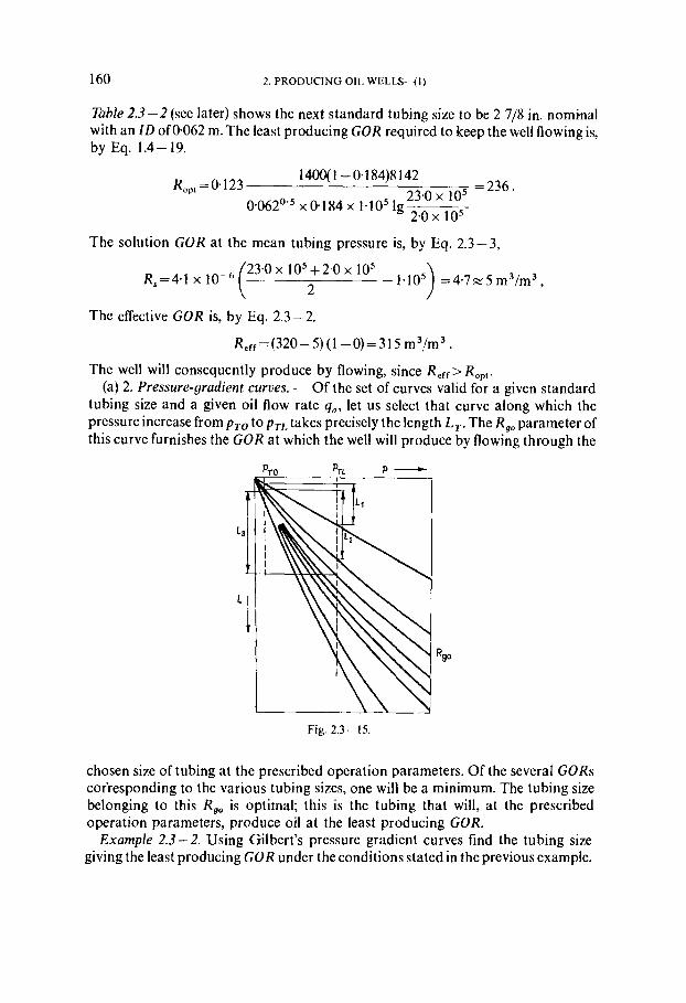
3-00 100 = 20.7 percent .
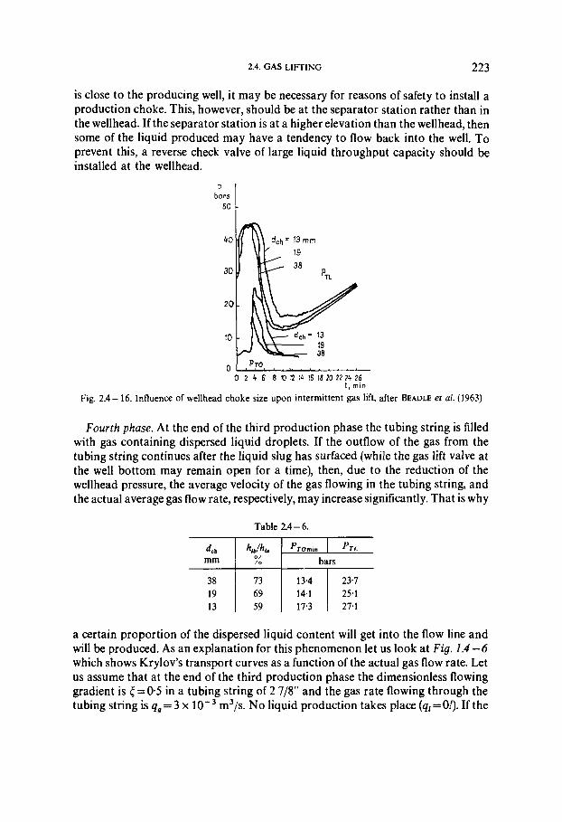
A careful consideration of the suitability of any formula selected for use is essential. A useful basis for such considerations is a series of tests carried out at the Institute of Gas Technology (Uhl 1967a). These tests have revealed a considerable difference between pipe in the laboratory and in the field. Its main cause is the considerable flow resistance due to pipe fittings, bends and breaks and weld seams in actual pipelines, which tend to bring about a modification of the Moody diagram.
The region of turbulent flow can be characterized by two types of equation. The first of these is the modified 'smooth-pipe' Equation 1.1 -6, valid for relatively low Reynolds numbers:
where 5 is a resistance factor accounting for the fittings, bends, breaks and weld seams per unit length of pipe, and A,, is the friction factor for smooth pipe, which can be calculated for any given value of NR,. At high Reynolds numbers, the relative roughness k / d , has a decisive influence on the friction factor. The latter can be calculated to a satisfactory degree of accuracy using Eq. 1.1 - 8. The two equations respectively characterize the transition and fully turbulent regions. The transition between them is appreciably shorter, more abrupt than in the case of the curves illustrating the Colebrook Formula 1.1 -7. The question as to which of the two equations (1.2- 14 or 1.1 -8) is to be used in any given case can be decided by finding the value of N,, that satisfies both equations simultaneously:
Determining the value of 5 requires in-plant or field tests. Approximate values are given in a diagram by Uhl (1967b).
We have so far assumed the mean values T, .5 and 1 to be constant all along the flow string. There are however, formulae that account also for changes of .T z and A along the string (Aziz 1962-1963). Among them, the calculation method of Cullender and Smith permits us to determine accurately the pressure drop of flow in a vertical string. The temperature is estimated from operational data. The calculation is based likewise on Eq. 1.2-2. which can be written to read
1.2. GAS FLOW IN PIPES 27
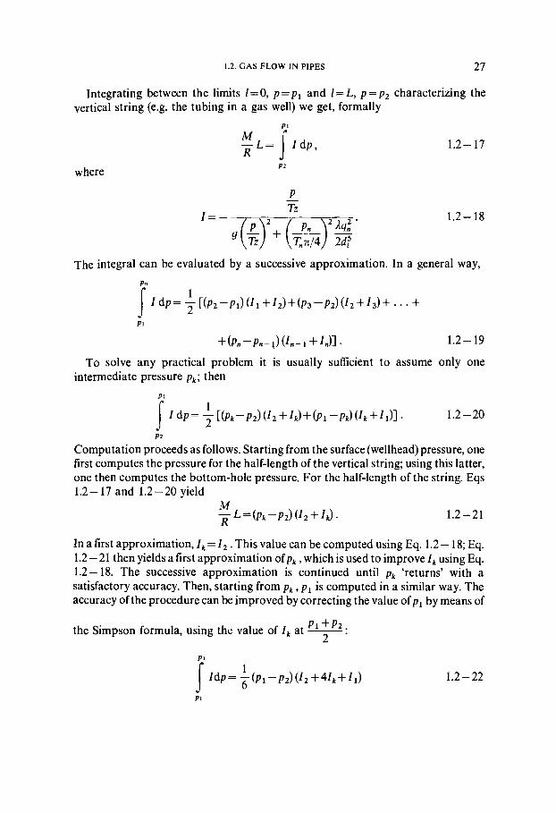
Integrating between the limits 1=0, p=p, and l = L , p=p2 characterizing the vertical string (e.g. the tubing in a gas well) we get, formally
PZ where
The integral can be evaluated by a successive approximation. In a general way,
To solve any practical problem it is usually sufficient to assume only one intermediate pressure p,; then
i 1 I dp= [ ( P ~ - P z ) ( ~ z + ~ ~ ) + @ I - P ~ ) ( ~ + ~ I ) ~ . 1.2-20
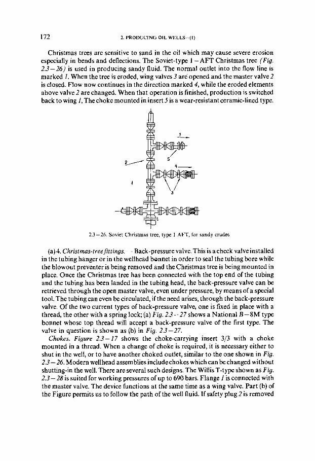
PZ
Computation proceeds as follows. Starting from the surface (wellhead) pressure, one first computes the pressure for the half-length of the vertical string; using this latter, one then computes the bottom-hole pressure. For the half-length of the string. Eqs 1.2-17 and 1.2-20 yield
In a first approximation, I, = I , . This value can be computed using Eq. 1.2 - 18; Eq. 1.2 -21 then yields a first approximation ofp, ,which is used to improve I, using Eq. 1.2-18. The successive approximation is continued until pk 'returns' with a satisfactory accuracy. Then, starting from p, , p, is computed in a similar way. The accuracy of the procedure can be improved by correcting the value of p, by means of
PI + P 2 . the Simpson formula, using the value of I, at - 2 .
28 I . SELECTED TOPIC'S I N FLOW MECHANICS
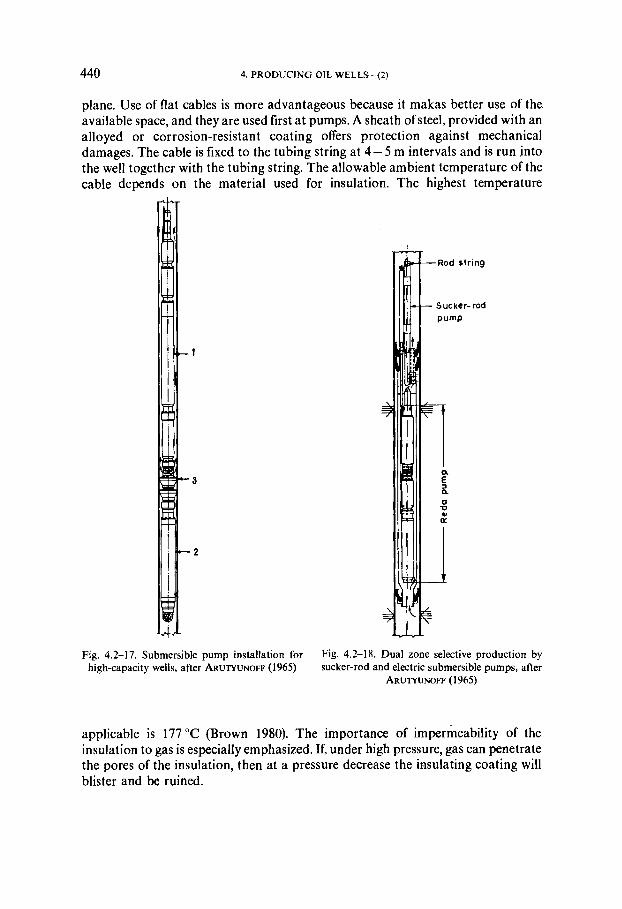
The friction factor may be computed from whichever formula is deemed most suitable; T, is an arithmetic or logarithmic mean estimated from operational measurements.
1.2.2. Pressure drop of gas flow in low-pressure pipes
The pressure drop of low-pressure gas flow can be calculated by means of the formulae discussed above but there exist simpler formulae that are just as satisfactory in most cases. Let p,= 1.01 3 bars, T,= 288.2 K, (p , + p,) x 2p,= 2-026 bars, f = I and ( p , -p,)=Ap. Substituting into 1.2-9 we get
A similar formula, which was used in American practice as.early as the last century, is that of Pole (Stephens and Spencer 1950); it yields with coefficients expressed in
M the SI system, and with y,= ---
28.96 '
Example 1.2-4. Find the gas flow rate in a pipeline if di=0.0266 m, 1 =420 m Ap = 2943 Pa, T= 288 K, M = 18-82 kg/kmole. By Eq. 1.2 - 23,
and by Eq. 1.2 -24,
1.2.3. Pressure drop of gas flow in high-pressure pipes
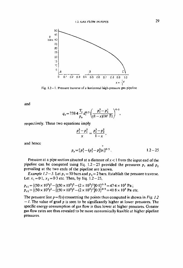
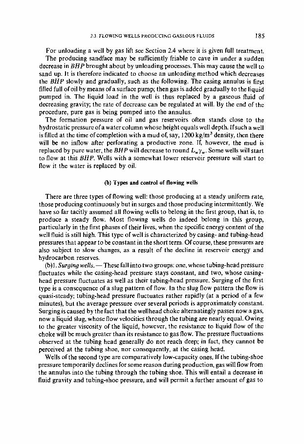
The gas pressure at various sections of pipelines, located at arbitrary distances from the input end, can be determined by the above formulae, e.g. approximately by Eq. 1.2-8. A pressure traverse can thus be established. An approximate pressure traverse can also be derived more simply, by assuming that the mean value z = 5 of the compressibility factor is constant all along the pipeline (Smirnov and Shirkovsky 1957). For the pipeline sections AB and BC in Fig. 1.2- 1, Eq. 1.2 -9 yields
1.2. GAS FLOW IN PIPES
P bors
w = h 1
Fig. 1.2- 1. Pressure traverse of a horizontal high-pressure gas pipeline
and
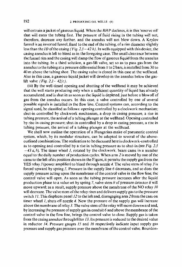
respectively. These two equations imply
and hence
Pressure at a pipe section situated at a distance of x< 1 from the input end of the pipeline can be computed using Eq. 1.2-25 provided the pressures p , and p, prevailing at the two ends of the pipeline are known.
Example 1.2-5. Let p , = 50 bars and p2 = 2 bars. Establish the pressure traverse. Let x, =0-1, x2 = 0.3 etc. Then, by Eq. 1.2 - 25,
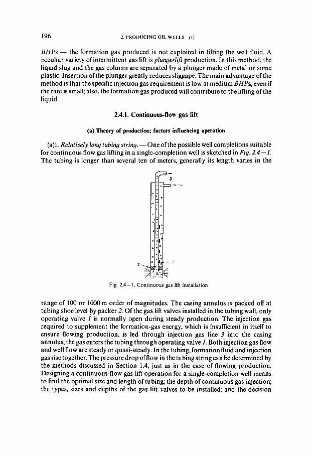
pxl = ((50 x 10')' - [(50 x -(2 x 10⁵)2]0.1)0'5 =47.4 x 10' Pa ; px2 = ((50 x 10')'-[(50 x 10')'-(2 x 10⁵)2]0.3)0.5 =41.8 x 10' Pa etc.
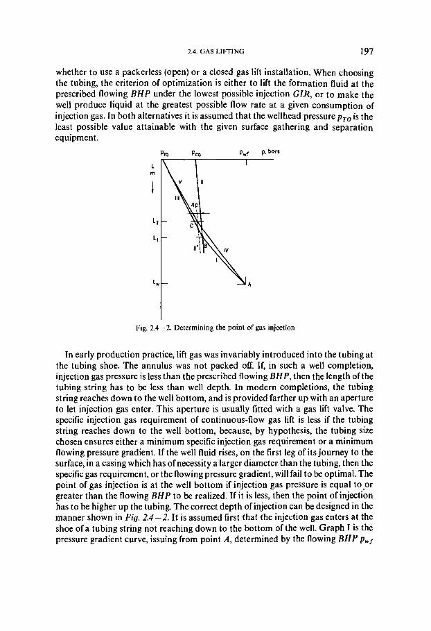
The pressure line p=f(x) connecting the points thus computed is shown in Fig. 1.2 - 1. The value of grad p is seen to be significantly higher at lower pressures. The specific energy consumption of gas flow is thus lower at higher pressures. Greater gas flow rates are thus revealed to be more economically feasible at higher pipeline pressures.
I . SELECTED TOPICS IN FLOW MECHANICS
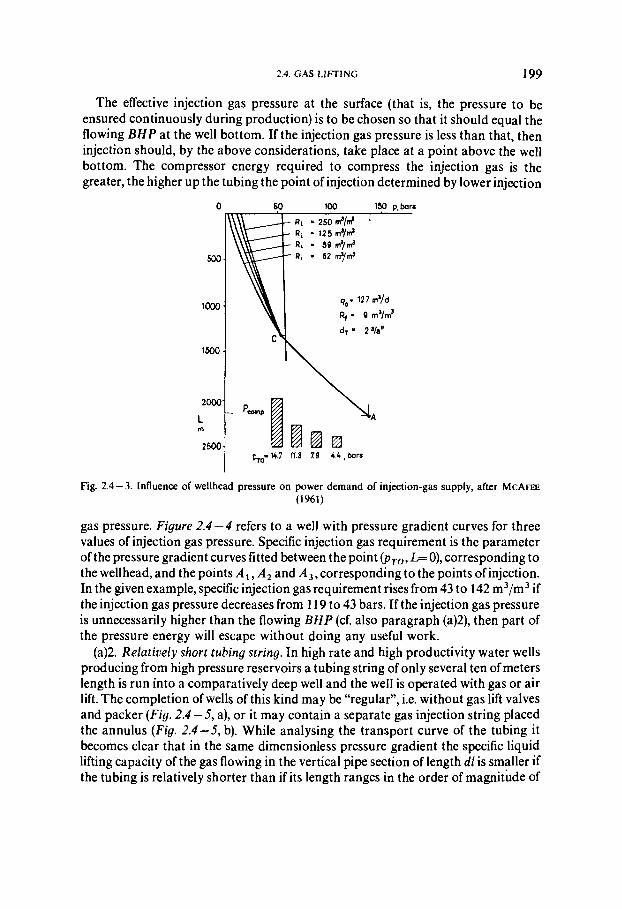
1.2.4. Mean pressure in gas pipes
The mean pressure in a gas pipeline is: 1
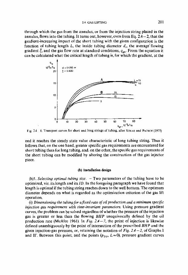
Substituting for px the approximate value given by Eq. 1.2 - 25 and solving for p, we obtain
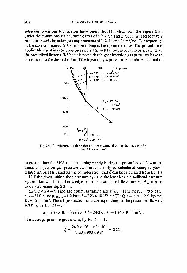
Example 1.2 - 6. Find the volume, in standard cubic metres of the gas contained in a pipeline if p, = 1.01 3 bars, T, = 288.2 K, p, = 50 bars, p2 = 25 bars, di = 0.1541 m, 1 = 36.2 km, T= 277.2 K, and M = 17.38 kg/kmole. Assuming z, = 1, the combined gas law gives
and
By Eq. 1.2-26, the mean pressure in the pipeline is
From diagram 8.1 -2, we read Y=089. Substitution of the values thus found into Eq. 1.2-27 yields
1.3. Flow of nowNewtonian fluids in pipes
1.3.1. Classification of fluids in rheology
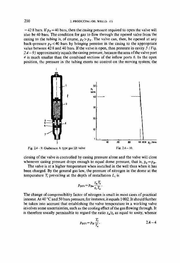
Fluids fall by their rheological properties into the following groups. (a) Purely viscous or time-independent fluids, whose viscosity is independent of the duration of shear. The group includes Newtonian fluids, whose viscosity is constant at a given pressure and temperature, as well as non-Newtonian fluids in the strict sense, whose apparent viscosity is a function of shear stress. (b) Time-dependent fluids, whose
1.3. FLOW OF NON-NEWTONIAN FLUIDS IN PIPES 3 1
apparent viscosity depends in addition to the shear stress also on the duration of the shear. (c) Viscoelastic liquids, whose apparent-viscosity is a function of both the shear stress and the extent of deformation. (d) Complex rheological bodies, &ibiting several of the properties of groups (a), (b) and (c).
By non-Newtonian fluids in the broader sense one means all fluids except the Newtonian ones. The oil industry most often has to deal with fluids of groups (a) and (b). Flow properties are characterized by flow curves or sets of such. Flow curves illustrate the variation of shear stress v. shear rate.
(a) Purely viscous fluids
To describe the flow curves of purely viscous fluids several mathematical models of phenomenological character may be used. The most widespread of them is the model created by Herschel], Porst, Moskowitsch and Houwink.
If T, = 0, then
D is the absolute value of the rate of shear. For a laminar flow in a pipe
This relation is the so-called power law of Ostwald and De Waele, which can be used to characterize the behaviour of some pseudoplastic (1 > n > 0) and dilatant (n> 1) fluids. At n = 1, this relationship simplifies to the equation
in the case of Newtonian fluids. If, in Eq. 1.3- 1, T,#O and n = I , then
This relationship is characteristic of plastic fluids, also called Bingham plastics. Let us note that in the subsequent equations factor p' of Eq. 1.3 - 1 turns up as a
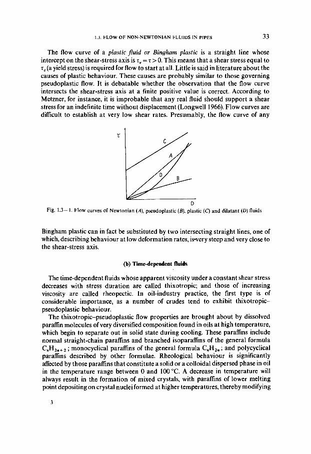
flow factor, denoted p', in 1.3 -2; as dynamic viscosity, denoted p, in 1.3 - 3; and finally as plastic or differential viscosity, denoted p", in 1.3 - 4. Flow curves of the types of fluid listed above are shown in Fig. 1.3- 1. The flow 'curve' of a Newtonian fluid is the straight line A, starting from the origin of coordinates.
Beside the "power law" shown in Eq. 1.3-2 other formulae are also used to model mathematically the flow curve of the pseudoplastic fluids. The more important formulae are shown in Table 1.3-1. The significance of the different descriptions generally lies only in the fact that between the related points T and D of
32 I . SELECTED TOPICS I N FLOW MECHANICS
Table 1.3- 1. Commonly used formulae for rheological models
Author Equation References
Herschell-Bulkley 7 - r , = a x D K Govier-Aziz (1 973)
Casson r 0 , 5 = a . g 0 . 5 + h Casson (1959)
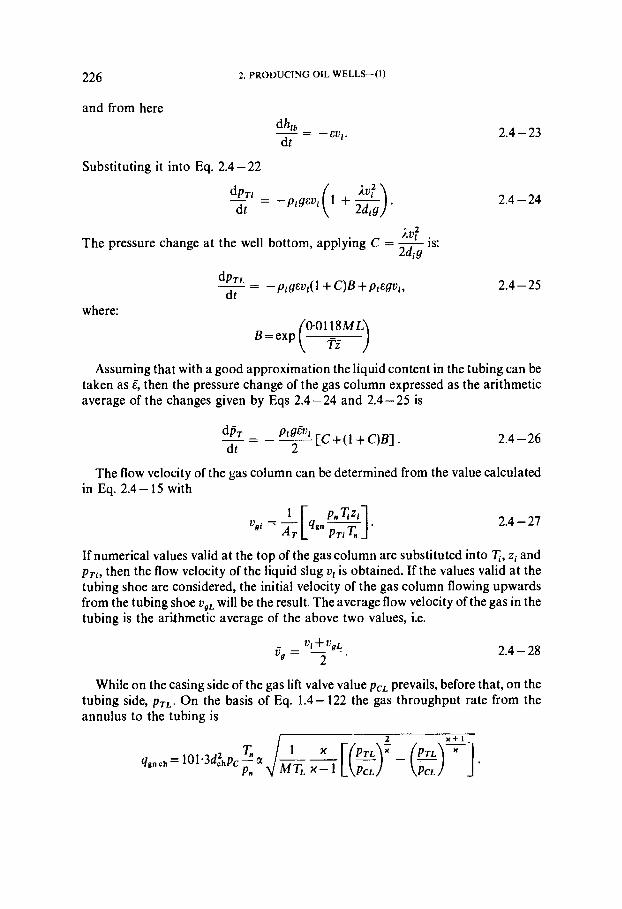
Prandtl-Eyring . = a x sinh1(;) Skelland (1967)
Powell-Eyring Skelland (1967)
Ellis
Sisko
Meter
Skelland (1967)
p = a + h x D ' " - " Sisko (1958)
Po-/& p = p m + ----- Meter-Bird (1964)
1 +(T/T,, ,)("-"
Note: descriptions of the parameters used in the above equations can be found in the references cited.
the given crudes, in certain cases one curve, and in other cases the other curve, calculated by different methods, can be applied with the proper accuracy in a longer run. The best known is the Ostwald-de Waele formula, shown in Eq. 1.3 - 3, which is a "power law" formula and which will also be used in the present study to interpret the pseudoplastic flow curves.
The characteristic behaviour ofpseudoplasticfluids, orfluids of structural viscosity, may be due to several causes. One simple interpretation of this behaviour is that in a liquid phase (serving as a dispersing medium) a solid dispersed phase of asymmetric particles is contained and shear will impress upon these randomly orientated particles a preferred orientation, with their major axes in the direction of shear. This preferred orientation will reduce the apparent viscosity. The term apparent
Z viscosity (pa) means for any non-Newtonian fluid the ratio - valid at a given shear
D rate. The typical flow curve, B in Fig. 1.3-1, likewise starts from the origin of coordinates, but its slope decreases as the deformation rate increases.
The flow curve of dilatant fluids, D in Fig. 1.3-1, is concave upward. The apparent viscosity thus increases as the shear rate increases. Dilatant behaviour is often encountered in wet sand whose properties were also studied by Reynolds himself. Increase of shear results in a progressive volume increase (dilatation) of the dispersed system because some of the moving sand grains enter into direct contact without a lubricating liquid film between them; so the apparent viscosity of the system increases. Dilatant behaviour is rare in crude oils, and even those few oils of this type have flow curves of insignificant curvature, so that the error due to regarding them as Newtonian and their flow curves as linear when calculating pressure drops is also insignificant (Govier and Ritter 1963).
1.3. FLOW OF NON-NEWTONIAN FLUIDS IN PIPES 33
The flow curve of a plastic fluid or Bingham plastic is a straight line whose intercept on the shear-stress axis is z,= r >O. This means that a shear stress equal to 7, (a yield stress) is required for flow to start at all. Little is said in literature about the causes of plastic behaviour. These causes are probably similar to those governing pseudoplastic flow. It is debatable whether the observation that the flow curve intersects the shear-stress axis at a finite positive value is correct. According to Metzner, for instance, it is improbable that any real fluid should support a shear stress for an indefinite time without displacement (Longwell 1966). Flow curves are difficult to establish at very low shear rates. Presumably, the flow curve of any
D Fig. 1.3- 1 . Flow curves of Newtonian (A), pseudoplastic (B), plastic (C) and dilatant (D) fluids
Bingham plastic can in fact be substituted by two intersecting straight lines, one of which, describing behaviour at low deformation rates, iwery steep and very close to the shear-stress axis.
(b) Time-dependent fluids
The time-dependent fluids whose apparent viscosity under a constant shear stress decreases with stress duration are called thixotropic; and those of increasing viscosity are. called rheopectic. In oil-industry practice, the first type is of considerable importance, as a number of crudes tend to exhibit thixotropic- pseudoplastic behaviour.
The thixotropic-pseudoplastic flow properties are brought about by dissolved paraffin molecules of very diversified composition found in oils at high temperature, which begin to separate out in solid state during cooling. These paraffins include normal straight-chain paraffins and branched isoparaffins of the general formula C,H,,+, ; monocyclical paraffins of the general formula C,H2,; and polycyclical paraffins described by other formulae. Rheological behaviour is significantly affected by those paraffins that constitute a solid or a colloidal dispersed phase in oil in the temperature range between 0 and 100 "C. A decrease in temperature will always result in the formation of mixed crystals, with paraffins of lower melting point depositing on crystal nuclei formed at higher temperatures, thereby modifying
34 I . SELECTED TOPICS IN FLOW MECHANICS
the crystal form of the original nucleus. The macroscopic structure of the separated paraffins may vary appreciably also with the rates of cooling. Rapid cooling produces a multitude of small independent crystal grains. Slow cooling gives rise to tabular, acicular and ribbon-like crystals which may aggregate to form a three- dimensional network. The shearing impact while cooling may contribute to the development of the network. The three-dimensional paraffin network may be significantly modified by.the asphaltene and maltene content of the oil, whereas other solids affect it to lesser extent. Asphaltene particles may serve as nuclei for parafin crystals, thus affecting the initial form of the paraffin structure. The maltenes have two main rheological effects: on the one hand, they keep the as- phaltenes in solution by their peptizing influence, and on the other, they may inhibit the formation of larger parafin crystals and thereby the formation of a coherent three-dimensional network by being adsorbed on paraffin crystals (Milley 1970).
Among the interpretations for the phenomenon of crude oil thixotropy the best known is the kinetic consideration by Govier and Ritter (Govier and Aziz 1973) founded on the analogy of the first- and second-order chemical reactions. Its essence is that the paraffin network, having already formed, breaks down as a result of shear effect under isothermal conditions but, simultaneously, the crystals in favoured places will try to unite. The system can resist shear effect best in an undisturbed condition with the resistance decreasing as the network breaks down. After time A t the realization frequency of bonds dividing and uniting under the effect of shear will be the same and apparent viscosity typical of flow properties is stabilized. The phenomenon is well characterized by isochronous flow curves, which, from among several values of shear stress obtained at a constant rate of shear, link those having the same duration of shear (F ig . 1.3-2). This theory furnished a good basis for solving several problems of the project concerning stabilized and partly transient flow in the pipeline. It is also used in the following parts of this work. During the latest research work of the author, however, it has become clear that this hypothesis cannot account for some flow occurrences, especially hysteresis. It is the gridshell theory that seems adequate to interpret these phenomena. The essence of this theory is as follows.
Under the effect of differences in velocities of the laminar flow established in an annular or circular space, crude oil decays into coaxial cylinders of thickness Ar. This is determined by the cross-sectional dimensions of paraffin-filaments. Along the generatrix of the annular cylinders, shells no shear effect is produced, only tangentially to the normal cross-section. The shape "pattern" of the lattice in an annular cylinder shell with good approximation corresponds to the cylinder-section of the original spacelattice, called shell-basis. To the shell-basis paraffin filaments are connected temporarily or durably in such way that at least one of their end is loose; they protrude from the shell-basis touching the neighbouring shell-basis, which rotates at a different rate. Under the effect of friction, one part of the divergent particles loses contact with the shell-basis, the other part bends on touching but remains linked to it. Phenomena, which could not be accounted for earlier, can be interpreted by the grid shell theory. Some significant and explainable features are:
1.3. FLOW OF NON-NEWTONIAN FLUIDS IN PIPES 3 5
the existence of stabilized hysteresis curve; there is no (or only very limited) space lattice regeneration during motion; in the course of relaxation anisotropic parafin network develops; the structural change of the oil and therefore the change of flow- ing behaviour due to shearing is irreversible under some circumstances; the flowing properties of the oil are influenced by shearing history (Szilas 1982, 1984).
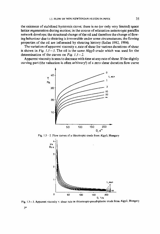
The variation of apparent viscosity v, rate of shear for various durations of shear is shown in Fiy. 1.3-3. The oil is the same Algyo crude which was used for the determination of the curves on Fig. 1.3-2.
Apparent viscosity is seen to decrease with time at any rate of shear. If the slightly curving part (the valuation is often arbitrary!) of a zero shear duration flow curve
I 0
t , rnin
1
Fig. 1.3-2. Flow curves of a thixotropic crude from Algyo, Hungary
P a s I
0 50 100 150 200 D, 11s
Fig. 1.3 - 3. Apparent viscosity v. shear rate in thixotropic-pseudoplastic crude from AlgyB, Hungary
36 I . SELECTED TOPICS I N FLOW MECHANICS
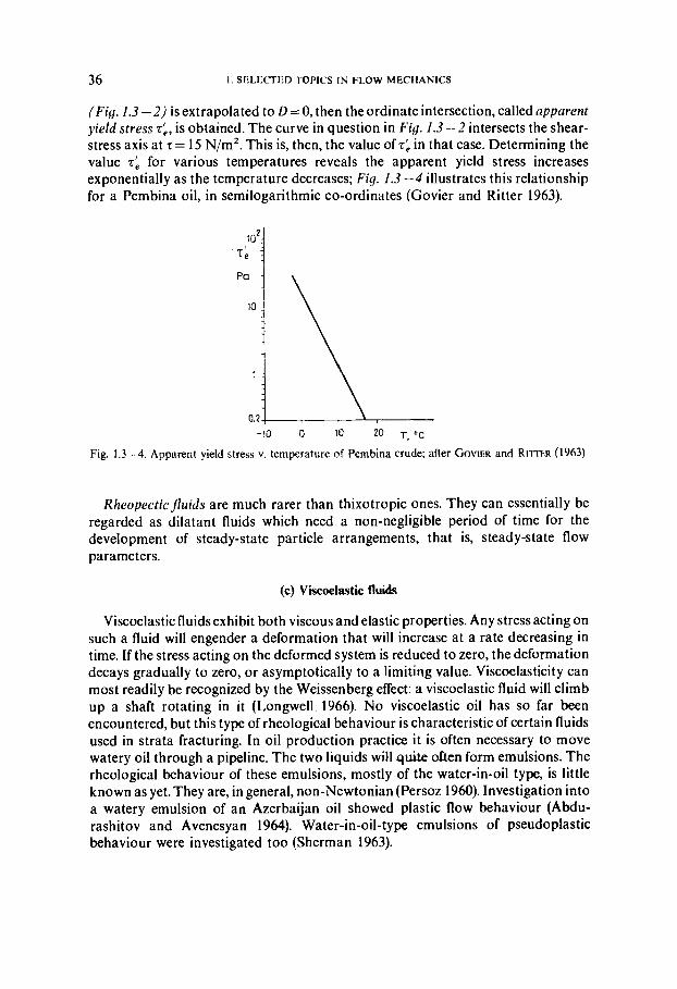
( F i g . 1.3 -2) is extrapolated to D = 0, then the ordinate intersection, called apparent yield stress zk, is obtained. The curve in question in Fig . 1.3 -2 intersects the shear- stress axis at z = 15 N/m2. This is, then, the value of z: in that case. Determining the value 2; for various temperatures reveals the apparent yield stress increases exponentially as the temperature decreases; Fig. 1.3-4 illustrates this relationship for a Pembina oil, in semilogarithmic co-ordinates (Govier and Ritter 1963).
-10 0 10 20 T, O c
Fig. 1.3-4. Apparent yield stress v. temperature of Pembina crude; after GOVIEK and RITTEK (1963)
Rheopect ic fluids are much rarer than thixotropic ones. They can essentially be regarded as dilatant fluids which need a non-negligible period of time for the development of steady-state particle arrangements, that is, steady-state flow parameters.
(c) Viscoelastic fluids
Viscoelastic fluids exhibit both viscous and elastic properties. Any stress acting on such a fluid will engender a deformation that will increase at a rate decreasing in time. If the stress acting on the deformed system is reduced to zero, the deformation decays gradually to zero, or asymptotically to a limiting value. Viscoelasticity can most readily be recognized by the Weissenberg effect: a viscoelastic fluid will climb up a shaft rotating in it (Longwell 1966). No viscoelastic oil has so far been encountered, but this type of rheological behaviour is characteristic of certain fluids used in strata fracturing. In oil production practice it is often necessary to move watery oil through a pipeline. The two liquids will quite often form emulsions. The rheological behaviour of these emulsions, mostly of the water-in-oil type, is little known as yet. They are, in general, nowNewtonian (Persoz 1960). Investigation into a watery emulsion of an Azerbaijan oil showed plastic flow behaviour (Abdu- rashitov and Avenesyan 1964). Water-in-oil-type emulsions of pseudoplastic behaviour were investigated too (Sherman 1963).
1.3. FLOW OF NON-NEWTONIAN FLUIDS IN PIPES
1.3.2. Velocity distribution in pipes
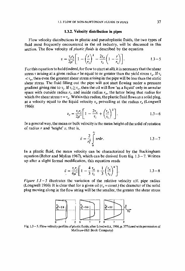
Flow velocity distributions in plastic and pseudoplastic fluids, the two types of fluid most frequently encountered in the oil industry, will be discussed in this section. The flow velocity of plastic fluids is described by the equation
For this equation to hold (indeed, for flow to start at all), it is necessary that the shear stress T arising at a given radius r be equal to or greater than the yield stress z,. If zi <T,, then even the greatest shear stress arising in the pipe will be less than the static shear stress. The fluid filling out the pipe will not start flowing under a pressure gradient giving rise to zi. If ti l z , , then the oil will flow 'as a liquid' only in annular space with outside radius r i , and inside radius re , the latter being that radius for which the shear stress z = z , . Within this radius, the plastic fluid flows as a solid plug, at a velocity equal to the liquid velocity v , prevailing at the radius r, (Longwell 1966):
In a general way, the mean or bulk velocity is the mean height of the solid of rotation of radius r and 'height' v, that is,
ri
vrdr.
0
In a plastic fluid, the mean velocity can be characterized by the Buckingham equation (Reher and Mylius 1967), which can be derived from Eq. 1.3-7. Written up after a slight formal modification, this equation reads
Figure 1.3-5 illustrates the variation of the relative velocity v /I . pipe radius (Longwell 1966). It is clear that for a given oil ( z , = const.) the diameter of the solid plug moving along in the flow string will be the smaller, the greater the shear stress
0 1 2 0 1 2 0 I 2
Fig. 1.3 - 5. Flow-velocity profiles of plastic fluids; after LONGWELL, 1966, p. 377 (used with permission of McGraw-Hill Book Company)
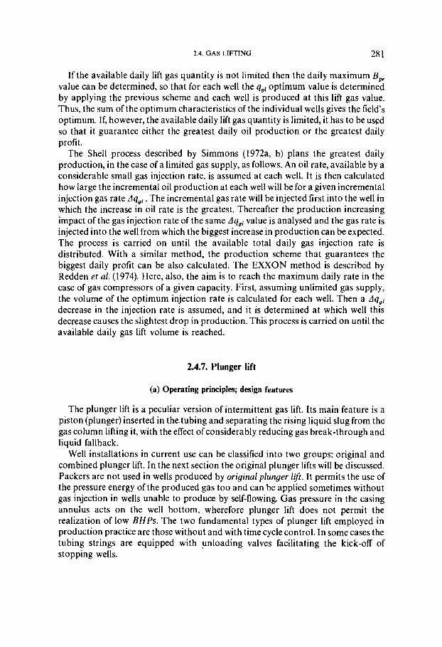
38 I . SELECTED TOPICS I N FLOW MECHANICS
at the pipe wall, that is, the greater the pressure gradient that keeps the fluid flowing. On the other hand, at a given pressure gradient and .ri engendered by it, the velocity distribution will approximate that of a Newtonian fluid the better, the 'less plastic' the fluid in flow, that is, the less the 7, value characterizing it.
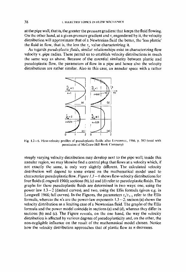
As regards pseudoplasticfluids, similar relationships exist in characterizing flow velocity v. pipe radius. These permit us to establish velocity distributions in much the same way as above. Because of the essential similarity between plastic and pseudoplastic flow, the parameters of flow in a pipe and hence also the velocity distributions are rather similar. Also in this case, an annular space with a rather
Fig. 1.3-6. Flow-velocity profiles of pseudoplastic fluids; after LONGWELL, 1966, p. 383 (used with permission of McGraw-Hill Book Company)
steeply varying velocity distribution may develop next to the pipe wall; inside this annular region, we may likewise find a central plug that flows at a velocity which, if not exactly the same, is only very slightly different. The calculated velocity distribution will depend to some extent on the mathematical model used to characterize pseudoplastic flow. Figure 1.3 - 6 shows flow-velocity distributions for four fluids (Longwell 1966); sections (b), (c) and (d) refer to pseudoplastic fluids. The graphs for these pseudoplastic fluids are determined in two ways: one, using the power law 1.3-2 (dashed curves), and two, using the Ellis formula (given e.g. in Longwell 1966; full curves). In the Figures, the parameters r i ,~ , , , refer to the Ellis formula, whereas the n's are the power-law exponents 1.3 -2; section (a) shows the velocity distribution as a limiting case of a Newtonian fluid. The graphs of the Ellis formula and the power model coincide in sections (a) and (d), whereas they differ in sections (b) and (c). The Figure reveals, on the one hand, the way the velocity distribution is affected by various degrees of pseudoplasticity and, on the other, the non-negligible influence on the result of the mathematical model chosen. Notice how the velocity distribution approaches that of plastic flow as n decreases.
1.3. FLOW OF NON-NEWTONIAN FLUIDS IN PIPES
1.3.3. The generalized Reynolds number
Let the shear stress in a fluid flowing in a pipe exceed the true or apparent static shear stress even in the centre line of the pipe; in this case, the flow will have no 'solid core', and the bulk velocity of flow will be correctly characterized by the general Eq. 1.3-7; from this equation the Wilkinson equation can be derived (Reher and Mylius 1967): li
It is verifiable that the expression on the left-hand side is, in Newtonian fluids, equal to the shear rate at the pipe wall, that is,
For pseudoplastic fluids, a formula describing the relation between the terms 8614 and (-duldr), had been derived by Rabinowitsch and Mooney. This formula was written by Metzner and Reed (1955) in the form
Substituting the expression for (-dvldr) into Eq. 1.3-2 we get
where
For laminar flow in a horizontal pipeline Eqs 1.1 - 1 to 1.1 -3 hold, provided NR, = N,,,, and putting v = 6. The general relationships
and
are also valid. Using these equations and Eqs 1.3 -2 and 1.3 - 11 of pseudoplastic flow, we may write up the generalized Reynolds number, derived by Metzner and Reed (1955), as
40 I . SELECTED TOPICS I N FLOW MECHANICS
By the above considerations, Eq. 1.3 - 15 is valid for pseudoplastic fluids obeying a power law, in which case p' and n are constant and are given numerically in the equation of the flow curve. Replacing p' in Eq. 1.3 - 15 by the expression in Eq. 1.3 - 13, we get
This formula is used if the rheological properties of the fluid have been determined by means of a capillary viscosimeter, or by field tests on a pipeline, or are known on the basis of a r i = f(8fi/di) curve. According to Eq. 1.3 - 12
if the fluid obeys the power law, then k and n are constants and their numerical values are known. The formula can, however, also be used if the fluid deviates from the power law. In this case it is sufficient to assume that Eq. 1.3 - 12 is the equation of the tangent to the r i = f(8E/di) curve plotted in an orthogonal bilogarithmic system of co-ordinates; n is the slope of the tangent and k is the ordinate belonging to the value (Soldi)= 1. The tangent should touch the curve at the point whose abscissa (8C/di) corresponds to the actual values of q and d i . If the flow behaviour is characterized by a zi = f(86/di) curve, then N,,,, can be derived even more simply by the following consideration (LeBaron Bowen 1961).
The apparent viscosity at the inner pipe wall is
T i p = - and p=vp. 86 - di
Substituting these expressions into Eq. 1.1 -2, we get
This relationship is of a general validity for all non-Newtonian fluids including pseudoplastic fluids deviating from the power law (where, obviously, NR,= N,,,,,). To find the Reynolds number by this equation, read the .ri belonging to the (Soldi) value corresponding to the intended 6 and di off an experimentally established zi=f(85/di) curve and substitute the appropriate data into Eq. 1.3- 18.
13.4. Transition from laminar to turbulent flow
The transition from laminar to turbulent flow in non-Newtonian fluids depends, in addition to the Reynolds number, also on a number of other factors affected by the rheological properties of the fluid. No general equation has been derived so far,
1.3. FLOW OF NON-NEWTONIAN FLUIDS IN PIPES 4 1
but individual research workers have published valuable partial results. Ryan and Johnson have introduced a stability parameter which has permitted them to write up the critical Reynolds number for pseudoplastic fluids obeying the power law as follows:
where
Assuming that NRe,=2100 in Newtonian fluids, the critical Reynolds number of pseudoplastic fluids varies in the range 2100 to 2400, depending on the exponent n of the power law (Longwell 1966).
Fig. 1.3-7. Laminar and turbulent flows in pipelines; after I<FBAKON BOWEN (1961)
Dodge and Metzner (1959) have found N,,,, to fall more or less into the domain of transition of Newtonian fluids and to increase slightly as n decreases. According to these authors, e.g., NRep,= 3100 at n=0.38.
According to Mirzadzhanzade et al. (1969), the development of turbulency depends to a significant extent on the particle size and concentration of the dispersed phase, as well as on the specific weight difference between the dispersing medium and the dispersed phase.
As the mathematical criteria established till now are far from unequivocal, it is expedient in doubtful cases to determine experimentally the type of flow prevailing under the intended flow conditions. The graphs in Fig . 1.3 - 7 have been determined experimentally (LeBaron Bowen 1961). Graph A characterizes laminar flow independently of pipe diameter. The set of Graphs B includes characteristic curves for turbulent flow in pipes of various diameters. The less the diameter, the greater the abscissa (86/di) at which flow becomes turbulent.
I . SELECTED TOPICS I N FLOW MECHANICS
1.3.5. Calculation of friction loss
(a) Laminar flow of pseudoplastic fluids
By Eq. 1.3 - 12, the shear stress developing at the pipe wall in a fluid flowing in a pipe is, at given values of k and n, a function of 80/di only. This consideration permits, with the possession of experimental data obtained by means of a capillary extrusion viscosimeter of capillary diameter d,, or in a flow test on a pipe, the direct calculation of the friction losses for any other pipe diameter.
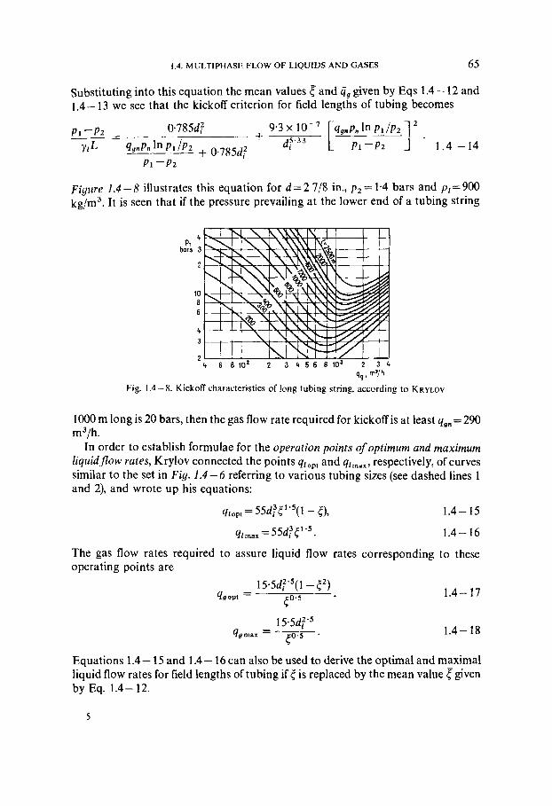
Example 1.3 - I . The variation of 7i = di grad 0. 86/di for a given oil is plotted 4
in Fig. 1.3 -8 on the basis of pipeline experiments. Find the pressure gradient in a pipe of d, =0.308 m, when q =200 m3/h at the given flow parameters.
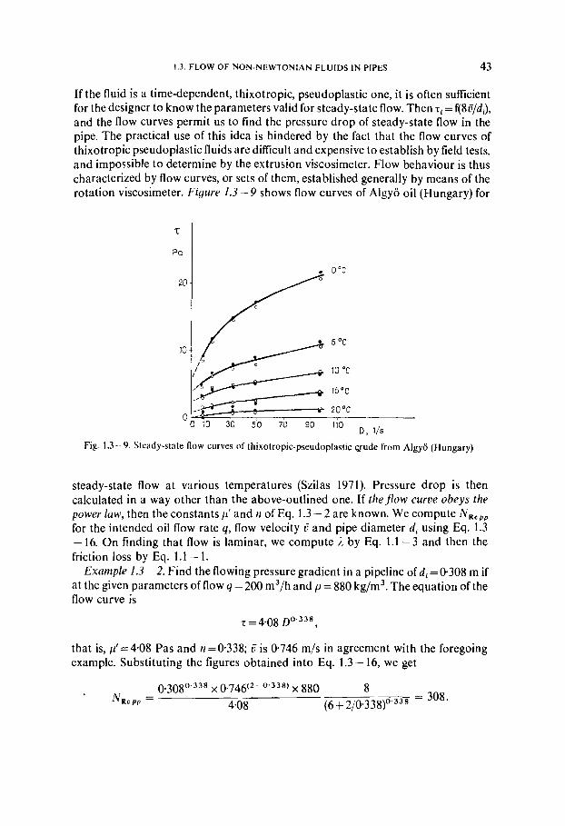
If the fluid is a time-dependent, thixotropic, pseudoplastic one, it is often sufficient for the designer to know the parameters valid for steady-state flow. Then .ri=f(86/di), and the flow curves permit us to find the pressure drop of steady-state flow in the pipe. The practical use of this idea is hindered by the fact that the flow curves of thixotropic pseudoplastic fluids are difficult and expensive to establish by field tests, and impossible to determine by the extrusion viscosimeter. Flow behaviour is thus characterized by flow curves, or sets of them, established generally by means of the rotation viscosimeter. Figure 1.3 - 9 shows flow curves of Algyo oil (Hungary) for
Fig. 1.3 - 9. Steady-state flow curves of thixotropic-pseudoplastic crude from Algyo (Hungary)
steady-state flow at various temperatures (Szilas 1971). Pressure drop is then calculated in a way other than the above-outlined one. If theflow curve obeys the power law, then the constants p' and n of Eq. 1.3 -2 are known. We compute N R e P p for the intended oil flow rate q, flow velocity 17 and pipe diameter di using Eq. 1.3 - 16. On finding that flow is laminar, we compute 1 by Eq. 1.1 -3 and then the friction loss by Eq. 1.1 - 1.
Example 1.3 -2. Find the flowing pressure gradient in a pipeline of di =0.308 m if at the given parameters of flow q = 200 m3/h and p = 880 kg/m3. The equation of the flow curve is
that is, pf=4.08 Pas and n=0.338; I7 is 0.746 m/s in agreement with the foregoing example. Substituting the figures obtained into Eq. 1.3 - 16, we get
44 I . SELECTED TOPICS IN FLOW MECHANICS
Flow is laminar, it is therefore justified to use Eq. 1.1 -3, which yields
Now by Eq. 1.1 -1,
A P / v2p grad p, = - = i- = 0.208 0.7462 x 880
1 = 165 N/m3 = 1.65 bar/km.
2di 2 x 0.308
If the flow curve does not obey the power law, then in Eq. 1.3- 16 p' means the ordinate intercept, at D = 1, of the tangent to the flow curve plotted in an orthogonal bilogarithmic system of coordinates, and n means the slope of said tangent. To find the deformation rate for which p' and n hold at the intended velocity 17 and pipe diameter d i , we may use Eq. 1.3 - 11 by Reed and Metzner (Govier and Ritter 1963). Calculation may proceed as follows: assuming several values of D, we determine the value of n belonging to each, using, on the one hand, Eq. 1.3 - 11 and, on the other, the tangents to the flow curves plotted in orthogonal bilogarithmic co-ordinates. The two functions are then plotted in a diagram. The desired value of n is given by their point of intersection. p' is furnished by the ordinate intercept at D = 1 of the tangent to the flow curve valid for the deformation rate belonging to this particular value of n.
(b) Turbulent flow of pseudoplastic fluids
The former formulae to define the pressure drop of turbulent flows were obtained either for smooth pipe, e.g. Dodge and Metzner (1959), Shaver and Merri11(1959), Tomita (Govier and Aziz 1973), or for rough pipes where, however, the roughness of the experimental pipes are "incorporated" in the constants in the formulae. This latter possibility was chosen by Clapp (Govier and Aziz 1973). The Bobok- Navratil-Szilas equation (later BNS)
was analytically derived and the friction factor is not only the function of the Reynolds number and the exponent of the power law, but also the function of the relative roughness k/di (Szilas et al. 1981). The formula can be interpreted as a generalized Colebrook formula and is valid for the turbulent transition zone. Its accuracy was tested by a series of experiments performed in a pipeline transporting pseudoplastic crude. It was found that in the Reynolds number ranges of lo4- 10'
1.3. FLOW OF NON-NEWTONIAN FLUIDS IN PIPES
L 1 2 4. Dodge-Metzner i 1.2
I - ;
5. CLAPP j 1- -1,48 + - Lg N 6 - 7 2:7 [ RePP (+) ] + ~ ( s n
0,30
Oa20
0,lO
0. 0
- 5 1 6. BNS; k l d i = 3 . 1 0
7. Shaver-Merrill j h =
- n = 0,60 $ = 000117 ~ s " l r n
2
9 = 820 kglm3
di = 0,3 m
-
-
- 7 100 200 300
9 [m3/h1
Fig. 1.3- 10. Pressure gradients of pseudoplast~c fluid flow after Szlu\s et al. (1981)
46 I . SELECTED TOPICS IN FLOW MECHANICS
the average absolute error was 4.1 percent, while the standard deviation, a, was 0.81 percent. In the experimental pipeline n varied between 0.5 and 1.0 and the temperature of the crude decreased from 43°C to 9°C.
As an example, Fig. 1.3 - I0 shows several curves (Apf/Al)di = f(q,),, calculated by using well-known methods from the literature. The same Figure shows pressure gradient-flow rate curves obtained with the BNS method for three different k/di relative roughness values of practical importance. It is clearly seen that the application of different equations leads to significantly differing values.
In the fully turbulent region N R , x w and then Eq. 1.3-21 is simplified to the Prandtl-Kannan formula, Eq. 1.1 -8. In this region the friction factor is not influenced by the flow parameters of the fluid and thus by the non-Newtonian flow behaviour. The boundaries of the fully turbulent region however will be different in cases of Newtonian and non-Newtonian crudes.
(c) Thixotropic pseudoplastic fluids
Figure 1.3-2 shows that the flow curve belonging to any shear duration of a thixotropic-pseudoplastic oil looks like the flow curve of a time-independent pseudoplastic oil. The flow curve belonging to infinite shear duration is consequently suitable for determining the flow parametefs of steady-state flow, and hence also the friction loss, in the way outlined in the previous paragraphs. In practice it is often found that after a shear duration in the order of 10 minutes the flow curve approximates quite closely the values to be expected at infinite duration of shear. In designing relatively long pipelines for pressure drop, accuracy is little influenced by the fact that the pressure gradient is slightly higher in a short section near the input end than the steady-state value in the rest of the pipeline. When, however, relatively short pipelines are to be designed for pressure drop, the error due to use of the steady-state pressure gradient may be quite considerable. A procedure for computing pressure drops under transient structural and flow conditions has been developed by Ritter and Baticky (1967).
(d) Plastic fluids
By the considerations in Section 1.3- 5(a), the pressure drop of a plastic fluid in laminar flow can also be determined in the way outlined in Example 1.3- 1, provided the graph of the function zi = f(8z7/di) has been determined experimentally, by means of an extrusion viscosimeter or by field tests. In the possession of a flow curve characterizing the behaviour of the fluid, the pressure drop can be calculated by. the following consideration. It has been shown by Hedstrom that the friction coefficient of plastic fluids is a function of two dimensionless numbers (Hedstrom 1952). One is a Reynolds number which involves the plastic viscosity p" in the place of the simple viscosity:
1.3. FLOW OF NON-NEWTONIAN FLUIDS IN PIPES
The other dimensionless number is named the Hedstrom number
This number accounts first and foremost for the fact that the 'soIid core' of the flow reduces the cross-section free for 'liquid' flow (LeFur and Martin 1967). - For flow
Fig. 1.3- 11. Friction factor of plastic fluids, according to HEDSTR~M (1952)
in a pipeline, the friction factor can be read from Fig. 1.3- 11 if N,,, and N,, are known (API 1960). The curve marked Tholds for turbulent flow; the rest hold for laminar flow. Let us add that the curve for turbulent flow refers to a smooth pipe and therefore gives approximate results only.
10 20 30 D, 1/e
Fig. 1.3 - 12.
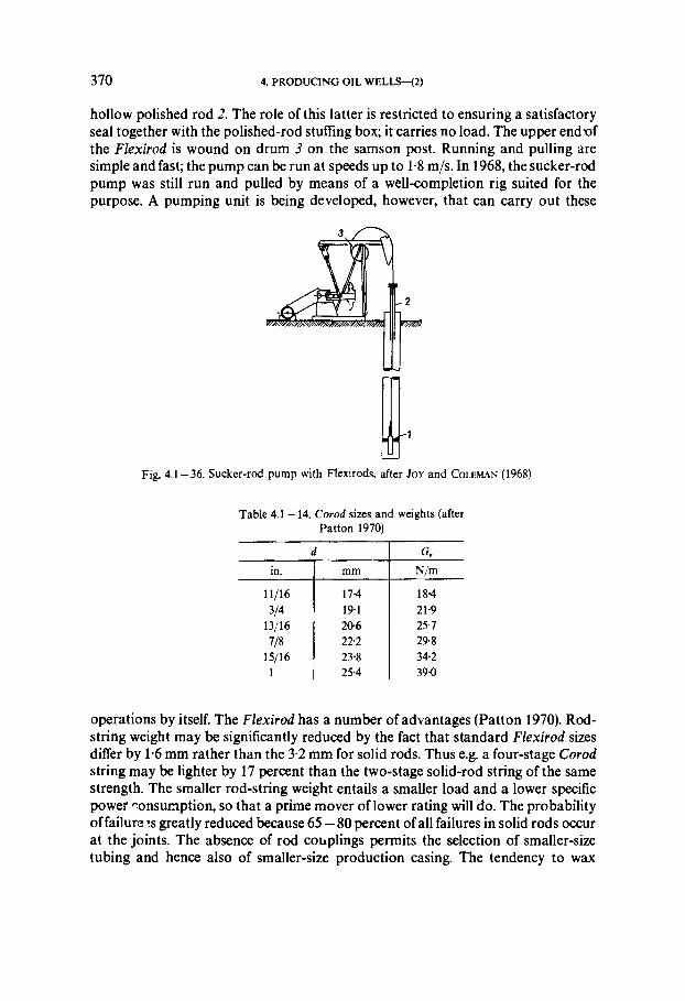
Example 1.3-3. Find the friction pressure gradient in the fluid characterized by flow curve in Fig. 1.3 - 12, if q = 200 m3/h, di =0.308 m and p = 880 kg/m3. - The flow curve yields .re = 8.6 Pa and, for instance at (- dv/dr) = 20 l/s, T = 1 1.4 Pa. Hence
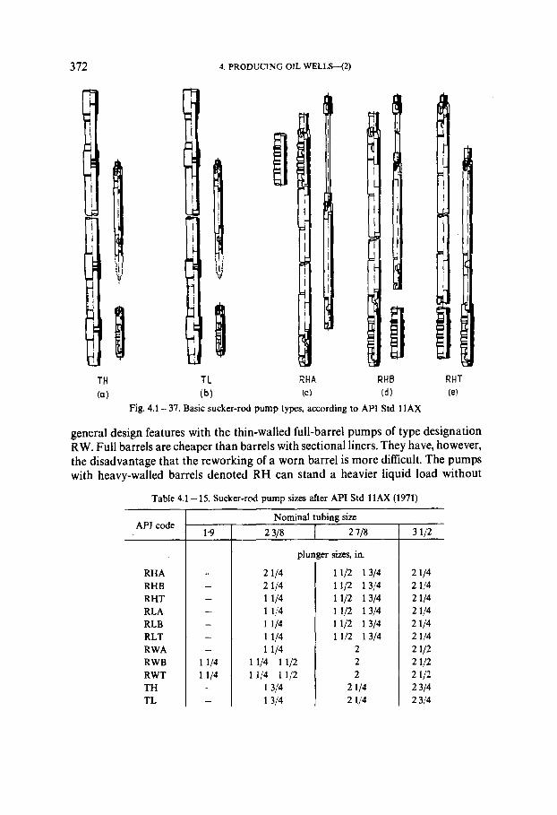
The basic condition of determining a representative flow curve is to ensure that the flow behaviour of the tested sample is the same as the fluid which will flow in the designed pipeline. In case of artificially made non-Newtonian fluids, e.g. in the case of fluids applied for hydraulic formation fracturing, the preparation of the samples are prescribed by special rules (API 1960).
The taking, transport, storage and preparation of thixotropic-pseudoplastic crude samples must be made with special care. Three main difficulties must be considered: (I) the dispersed phase settles out in the dispersion medium; (2) the light hydrocarbon components are evaporating while storing; (3) the flow behaviour characteristics can be significantly influenced by the temperature and shear history (Szilas 1971).
For the measurement of flow curves extrusion or rotary viscometers are generally applied.
(a) Measurements with extrusion viscometers
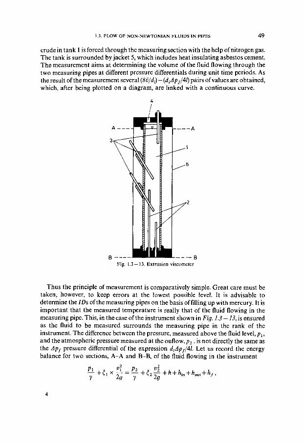
The extrusion viscometer is the type of capillary or discharge viscometer where the fluid to be measured flows in the measuring section not because of gravity but due to the pressure differential occurring at the two ends of the measuring pipe section. Many types and models of extrusion viscometers are known. In the following section (after Le Baron Bowen 1961) we shall speak of a model suitable to measure pseudoplastic crudes.
The length of tank 1 of the extrusion viscosimeter shown on Fig. 1.3-13 is 610 mm, its inside diameter is 76 mm and it can be used with an allowed internal overpressure of 10 bars. Two stainless steel measuring pipes of different lengths (2) are mounted in the tank. Their IDS are 1.6 mm and 3.2 mm, respectively. They are fixed to the bottom of the tank. The temperature is measured with three thermometers, 3, each having a measuring accuracy of 0.1 "C. Through hole 4 the
1.3. FLOW OF NON-NEWTONIAN FLUIDS IN PIPES 49
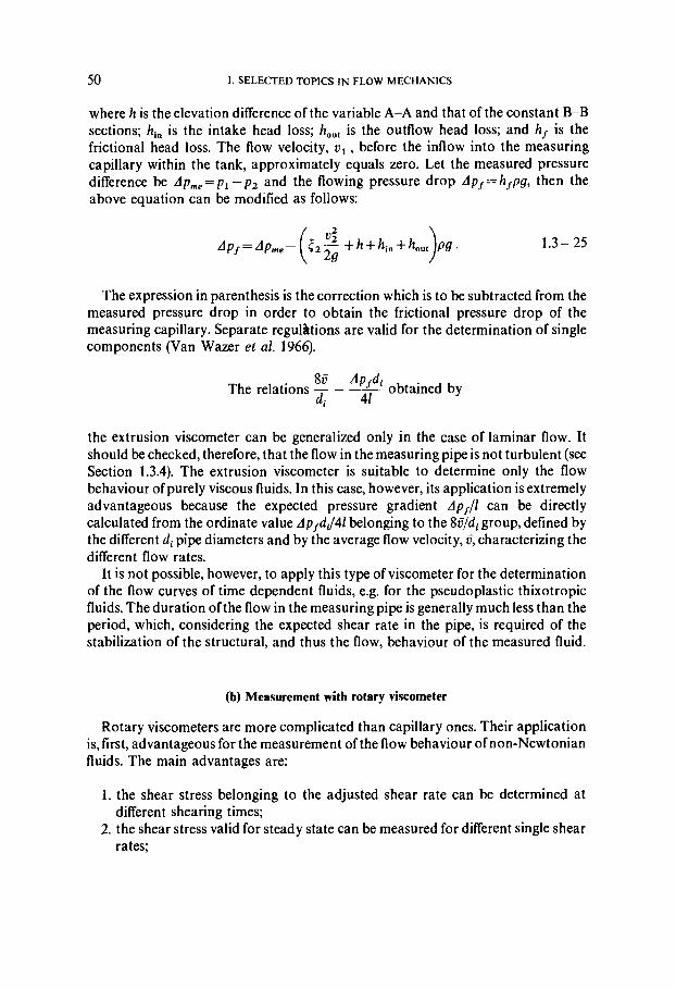
crude in tank 1 is forced through the measuring section with the help of nitrogen gas. The tank is surrounded by jacket 5, which includes heat insulating asbestos cement. The measurement aims at determining the volume of the fluid flowing through the two measuring pipes at different pressure differentials during unit time periods. As the result of the measurement several (@Idi) - (diAp f/41) pairs of values are obtained, which, after being plotted on a diagram, are linked with a continuous curve.
Fig. 1.3 - 13. Extrusion viscometer
Thus the principle of measurement is comparatively simple. Great care must be taken, however, to keep errors at the lowest possible level. It is advisable to determine the IDS of the measuring pipes on the basis of filling up with mercury. It is important that the measured temperature is really that of the fluid flowing in the measuring pipe. This, in the case of the instrument shown in Fig. 1.3 - 13, is ensured as the fluid to be measured surrounds the measuring pipe in the rank of the instrument. The difference between the pressure, measured above the fluid level, p,, and the atmospheric pressure measured at the ouflow, p2 , is not directly the same as the Apf pressure differential of the expression diApf/41. Let us record the energy balance for two sections, A-A and B-B, of the fluid flowing in the instrument
50 I . SELECTED TOPICS IN FLOW MECHANICS
where h is the elevation difference of the variable A-A and that of the constant B-B sections; hi, is the intake head loss; h,,, is the outflow head loss; and h, is the frictional head loss. The flow velocity, v , , before the inflow into the measuring capillary within the tank, approximately equals zero. Let the measured pressure difference be Ap,,=p, -p2 and the flowing pressure drop ApJ-hfpg, then the above equation can be modified as follows:
The expression in parenthesis is the correction which is to be subtracted from the measured pressure drop in order to obtain the frictional pressure drop of the measuring capillary. Separate regulbtions are valid for the determination of single components (Van Wazer et al. 1966).
The relations - !-!@ obtained by di 41
the extrusion viscometer can be generalized only in the case of laminar flow. It should be checked, therefore, that the flow in the measuring pipe is not turbulent (see Section 1.3.4). The extrusion viscometer is suitable to determine only the flow behaviour of purely viscous fluids. In this case, however, its application is extremely advantageous because the expected pressure gradient ApJ/l can be directly calculated from the ordinate value ApJd,/41 belonging to the 8C/di group, defined by the different di pipe diameters and by the average flow velocity, 6, characterizing the different flow rates.
It is not possible, however, to apply this type of viscometer for the determination of the flow curves of time dependent fluids, e.g. for the pseudoplastic thixotropic fluids. The duration of the flow in the measuring pipe is generally much less than the period, which, considering the expected shear rate in the pipe, is required of the stabilization of the structural, and thus the flow, behaviour of the measured fluid.
(b) Measurement with rotary viscometer
Rotary viscometers are more complicated than capillary ones. Their application is, first, advantageous for the measurement of the flow behaviour of non-Newtonian fluids. The main advantages are:
1. the shear stress belonging to the adjusted shear rate can be determined at different shearing times;
2. the shear stress valid for steady state can be measured for different single shear rates;
1.3. FLOW OF NON-NEWTONIAN FLUIDS IN PIPES 51
3. the shear stress of the same sample can be determined at different shear rates. Thus due to the above features the instrument is suitable to determine the flow behaviour of time dependent fluids;
4. the shear rate of the fluid sample in the viscometer only varies slightly, so it is possible to obtain the shear stress valid at the given shear rate. (In the case of the extrusion viscometer the shear rate and the shear stress vary considerably along the radius of the measuring pipe. The value of the measured shear stress is valid on the pipe wall.)
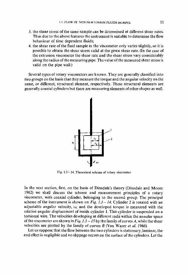
Several types of rotary viscometers are known. They are generally classified into two groups on the basis that they measure the torque and the angular velocity on the same, or different, structural element, respectively. These structural elements are generally coaxial cylinders but there are measuring elements of other shapes as well.
Fig. 3.3- 14. Theoretical schema of rotary viscometer
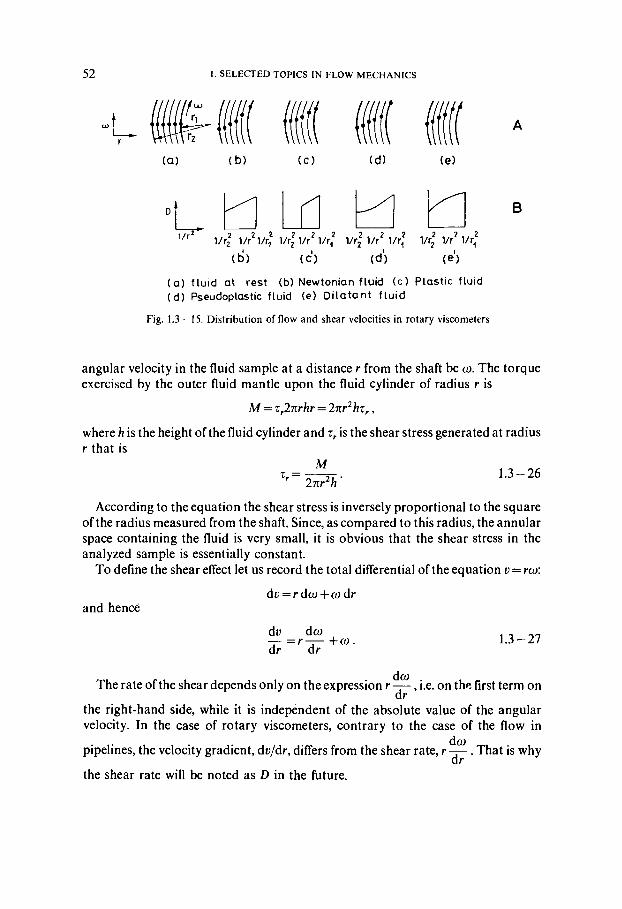
In the next section, first, on the basis of Dinsdale's theory (Dinsdale and Moore 1962) we shall discuss the scheme and measurement principles of a rotary viscometer, with coaxial cylinder, belonging to the second group. The principal scheme of the instrument is shown on Fig. 1.3- 14. Cylinder 2 is rotated with an adjustable angular velocity, o, and the developed torque is measured with the relative angular displacement of inside cylinder 1. This cylinder is suspended on a torsional wire. The velocities developing at different radii within the annular space ofthe viscometer are shown in Fig. 1.3 - 15 by the family ofcurves A, while the shear velocities are plotted by the family of curves B (Van Wazer et al. 1966).
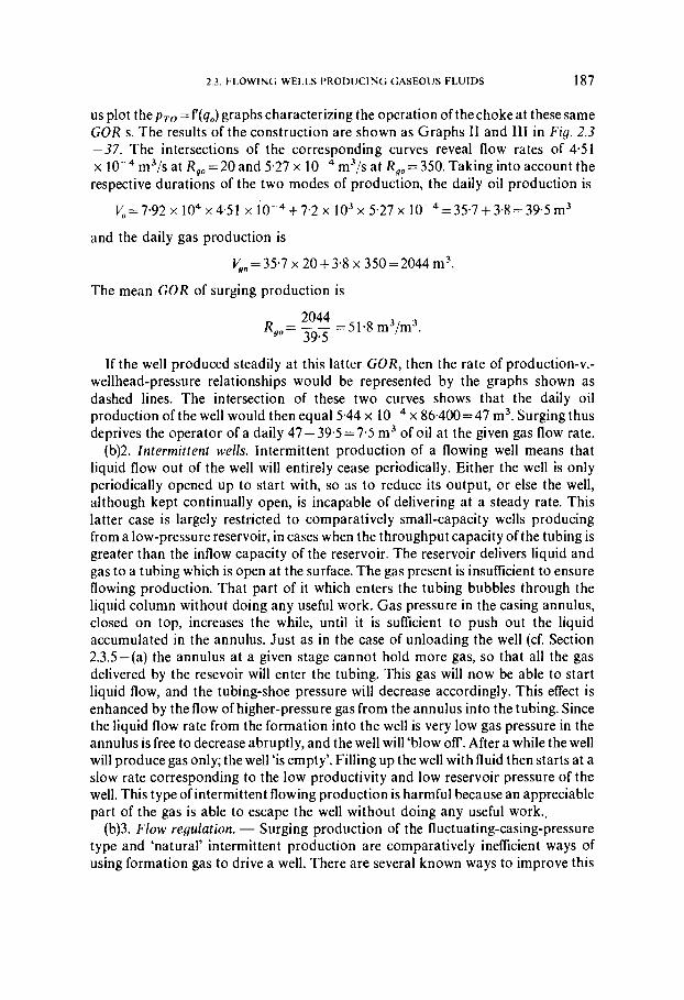
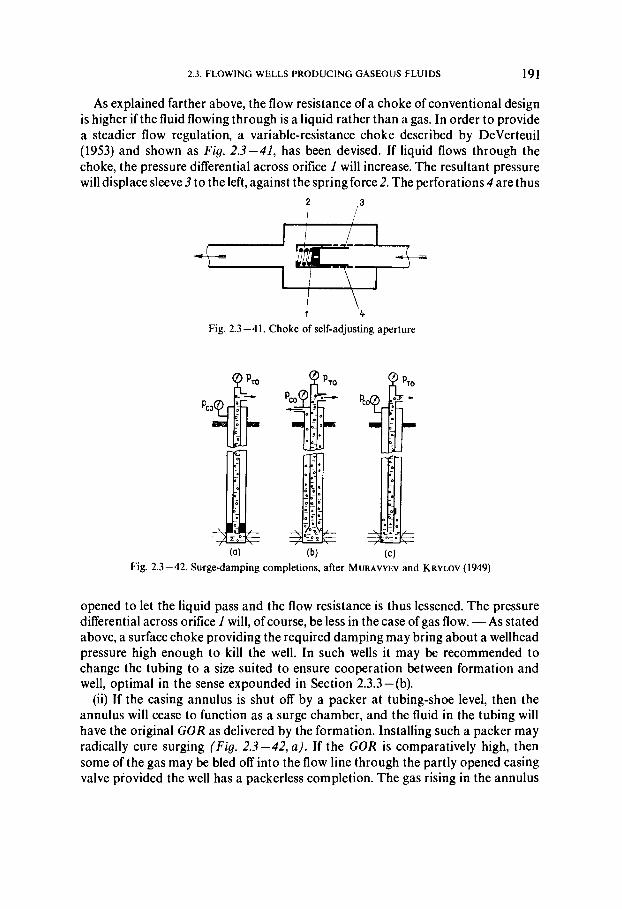
Let us suppose that the flow between the two cylinders is stationary, laminar, the end effect is negligible and no slippage occurs on the surface of the cylinders. Let the
52 I . SELECTED TOPICS I N FLOW MECHANICS
(a) f l u ~ d at res t (b) Newtonian fluid ( c ) Plastic fluid ( d ) Pseudoplastic fluid (e) Dilatant fluid
Fig. 1.3- 15. Distribution of flow and shear velocities in rotary viscometers
angular velocity in the fluid sample at a distance r from the shaft be w. The torque exercised by the outer fluid mantle upon the fluid cylinder of radius r is
where h is the height of the fluid cylinder and rr is the shear stress generated at radius r that is
According to the equation the shear stress is inversely proportional to the square of the radius measured from the shaft. Since, as compared to this radius, the annular space containing the fluid is very small, it is obvious that the shear stress in the analyzed sample is essentially constant.
To define the shear effect let us record the total differential of the equation u =ro:
d v = r d o + w d r and heno5
d o The rate of the shear depends only on the expression r - , i.e. on the first term on
dr the right-hand side, while it is independent of the absolute value of the angular velocity. In the case of rotary viscometers, contrary to the case of the flow in
d o pipelines, the velocity gradient, duldr, differs from the shear rate, r - . That is why
dr the shear rate will be noted as D in the future.
1.3. FLOW OF NON-NEWTONIAN FLUIDS IN PIPES
For Newtonian fluids Z, = pD, and thus by applying Eqs 1.3 - 26 and 1.3 - 27
and then
We assume that no slippage occurs on the pipe walls, i.e. if r = r , , then w =O; and at r = r , the angular velocity, w, equals the angular velocity of the rotating cylinder. These are the boundary conditions with which we solve the equation, from which the torque
where C is an instrument constant depending on the geometrical parameters of the instrument.
The equation is also valid if the internal cylinder is rotated with an angular velocity, o , and the outer cylinder is suspended on a torsional wire, or if the rotated cylinder is also a structural element suspended on the torsional wire.
The average shear rate and average shear stress can be determined either as an arithmetic or as a geometric mean. In the first case, considering Eq. 1.3 -26, the mean shear stress is
and f= pD, respectively, and on the basis of Eqs 1.3 - 28 and 1.3 - 29 the arithmetic mean of the shear rate is
* A
The geometric mean values are
and
respectively. The above equations are valid, generally, only for the fluids of Newtonian
behaviour. If, however, the annular space between the two cylinders is small enough, they can be applied for non-Newtonian fluids as well. A measuring instrument of this type is, for example, the Haake type rotary viscometer discussed below, which is
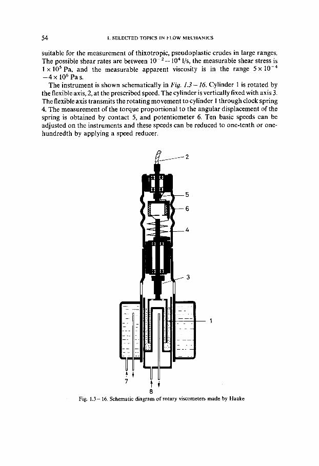
54 1. SELECTED TOPICS IN FLOW MECHANICS
suitable for the measurement of thixotropic, pseudoplastic crudes in large ranges. The possible shear rates are between lo-'- lo4 I/s, the measurable shear stress is 1 x 10⁵Pa, and the measurable apparent viscosity is in the range 5 x - 4 x lo6 Pas.
The instrument is shown schematically in Fig. 1.3 - 16. Cylinder 1 is rotated by the flexible axis, 2, at the prescribed speed. The cylinder is vertically fixed with axis 3. The flexible axis transmits the rotating movement to cylinder 1 through clock spring 4. The measurement of the torque proportional to the angular displacement of the spring is obtained by contact 5, and potentiometer 6. Ten basic speeds can be adjusted on the instruments and these speeds can be reduced to one-tenth or one- hundredth by applying a speed reducer.
Fig. 1.3 - 16. Sch 8
~ematic diagram of rotary viscometers made by
1.4. MULTIPHASE FLOW OF LIQUIDS AND GASES
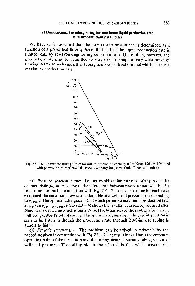
1.4. Multiphase flow of liquids and gases
1.4.1. Flow in vertical pipe strings
(a) Introduction
Research into the laws governing two-phase vertical flows has long been pursued. Versluys (1930) was the first to give a general theory. Numerous new theories have been published since, and, although research cannot be regarded as complete, we are today in possession of formulae of satisfactory accuracy for the flow regions important in practice. These formulae are based on various theoretical approaches, and in solving various problems or explaining various phenomena encountered in oil and gas production the formula that is frequently changes. The reasons why the relationships describing two-phase vertical flow so complicated are (a) that the specific volume of the flowing fluid varies appreciably as a function of pressure and temperature, (b) slippage losses arise in addition to friction losses, (c) flow is affected by a great number of parameters and (d) liquid and gas may assume a variety of flow patterns. The problems of flow will be discussed below with the main emphasis on wells producing a gaseous liquid.
(A) The specific volume of gas gradually increases as it surges upwards, owing to the decrease of the pressure acting on it. This is due, on the one hand, to the expansion of the free gas entering at the tubing shoe and, on the other, to the escape of more and more dissolved gas from the flowing oil under the decreasing pressure. Both effects are mitigated by the decrease in temperature. The specific volume of oil will decrease slightly owing to the escape of gas and to the decrease in temperature and increase slightly owing to the decrease in pressure.
(B) Two-phase vertical flow involves two types of energy loss: friction loss and slippage loss. Friction loss is an energy loss similar to that which arises in single- phase turbulent flows. The velocity distribution over the cross-section of the flow string, which considerably affects friction is, however, significantly influenced by the flow pattern. In the course of upward flow, moreover, the friction factor may vary considerably because the relative gas content of the fluid in contact with the pipe well and the flow velocity both increase monotonously. Hence, even if the only loss to be reckoned with were due to friction, we should be faced with much more of a problem than in the case of single-phase flow. The energy loss of flow is, however, further complicated by the phenomenon of slippage. Slippage loss is due primarily to the great difference in specific weight between the gas and the liquid. The gas bubble entering the flow string at the tubing shoe will leave the liquid element entering with it far behind.
Slippage loss can be considered zero, when the velocity of the elements of the rising liquid are exactly the same as that of the gas bubbles in it. Let the cross-section of the pipe be " A . Now the total mass of the fluid filling 1 m of this pipe will be
56 I . SELECTED TOPICS I N FLOW MECHANICS
From this equation the average density of the liquid-gas mixture is:
= pdl -&,I + P,E , . 1.4- 1
Example. When p, = 1000 kg/m3, p,= 10 kg/m3 and E, =0.66, the density of the mixture will be p, = 1000 (1 -0.66)+ 10 x 0.66 = 347 kg/m3.
Let us suppose now that the velocity v, of the gas is increased to k x v, with both the gas-flow rate (4,) and the liquid flow rate (q,) being kept constant. Since
it is quite obvious that such increase in velocity will necessarily result in a decrease of the gas-filled volume of the section from E, to ~ ~ / k .
The average density of the mixed gas-liquid flow will then be described by
Taking the figures of the above example and assuming that k is equal to 1.2 the average density of the mixture will be
that is, the phenomenon of slippage resulted in an increase of the density, and, thus, also in an increase of the mass of the fluid column, that fills the tubing. To lift this excess mass needs, of course, additional energy during production. Slippage loss is great in the case of relatively low gas-flow rates in relatively large diameter tubings.
Let the liquid flow rate through section A of the flow string situated at a given depth be q, and let the effective gas flow rate be q,. Let a fraction E, of the section be filled with liquid and the rest, ( 1 - E , ) = E , by gas. The flow velocity of the liquid is
and that of the gas is
The slippage velocity, proportional to the slippage loss is, then
(C) The pressurz gradient of flow, also called the flow gradient, is affected by a host of independent variables. Ros (1961) has listed 12 such factors ( I D of tubing; relative roughness of pipe well; inclination of the tubing to the vertical; flow velocity, density,
1.4. MULTIPHASE FLOW OF LIQUIDS AND GASES 57
viscosity of both liquid and gas; interface tension; wetting angle; acceleration of gravity). There are further factors, e.g. flow temperature, whose influence can at best be estimated.
(D) The spatial arrangement relative to each liquid and gas and the filling-out of space by the individual phases, may take a variety of forms. The typical
Fig. 1.4 -
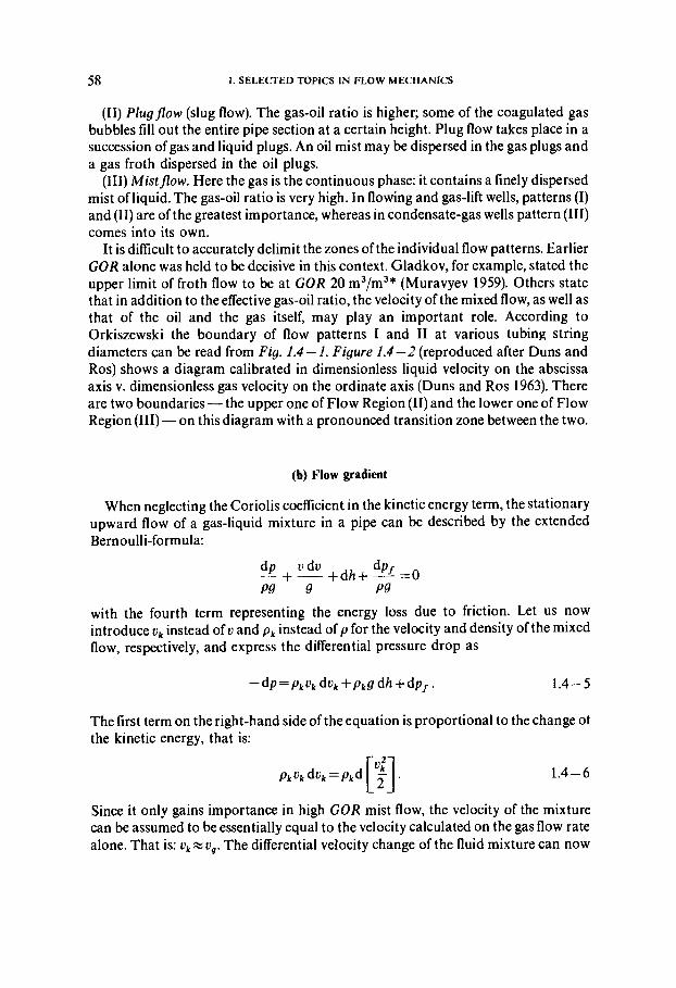
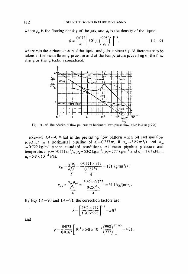
Fig. 1.4-2. Boundaries of flow patterns and the transition region after DUNS and Ros (1963)
arrangements are called flow patterns. There is no full agreement in literature as to the classification of flow patterns. The following classification seems to be the most natural.
(I) Frothflow. The continuous liquid phase contains dispersed gas bubbles. The number and size of gas bubbles may vary over a fairly wide range, but the gas-oil ratio is usually less than in the other flow patterns. If the gas bubbles move more or less parallel to the centre line of the pipe, the flow is called bubble flow, whereas in froth flow in the strict sense of the term, the bubbles are in turbulent motion.
58 I. SELECTED TOPICS IN FLOW MECHANICS
(11) Plugflow (slug flow). The gas-oil ratio is higher; some of the coagulated gas bubbles fill out the entire pipe section at a certain height. Plug flow takes place in a succession of gas and liquid plugs. An oil mist may be dispersed in the gas plugs and a gas froth dispersed in the oil plugs.
(111) Mistflow. Here the gas is the continuous phase: it contains a finely dispersed mist of liquid. The gas-oil ratio is very high. In flowing and gas-lift wells, patterns (I) and (11) are of the greatest importance, whereas in condensate-gas wells pattern (111) comes into its own.
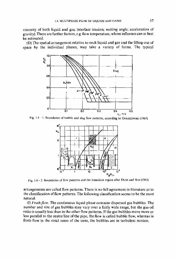
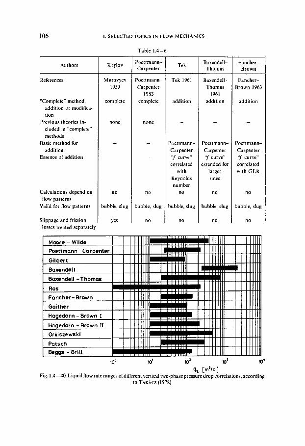
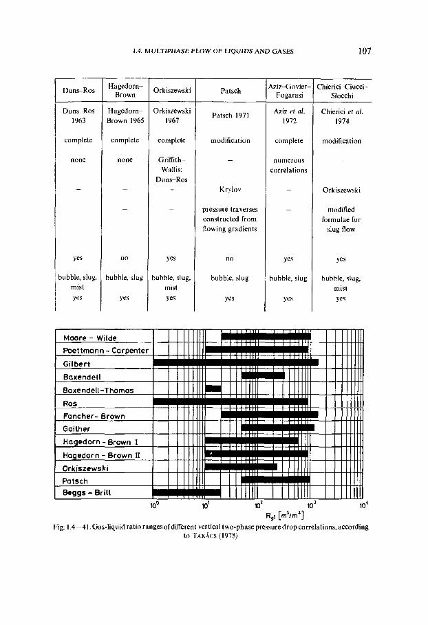
It is difficult to accurately delimit the zones of the individual flow patterns. Earlier GOR alone was held to be decisive in this context. Gladkov, for example, stated the upper limit of froth flow to be at GOR 20 m3/m3* (Muravyev 1959). Others state that in addition to the effective gas-oil ratio, the velocity of the mixed flow, as well as that of the oil and the gas itself, may play an important role. According to Orkiszewski the boundary of flow patterns I and I1 at various tubing string diameters can be read from Fig. 1.4- I. Figure 1.4-2 (reproduced after Duns and Ros) shows a diagram calibrated in dimensionless liquid velocity on the abscissa axis v. dimensionless gas velocity on the ordinate axis (Duns and Ros 1963). There are two boundaries - the upper one of Flow Region (11) and the lower one of Flow Region (111) -on this diagram with a pronounced transition zone between the two.
(b) Flow gradient
When neglecting the Coriolis coefficient in the kinetic energy term, the stationary upward flow of a gas-liquid mixture in a pipe can be described by the extended Bernoulli-formula:
dp vdu dpf - + - +dh+ - = O PS 9 PS
with the fourth term representing the energy loss due to friction. Let us now introduce vk instead of o and pk instead of p for the velocity and density of the mixed flow, respectively, and express the differential pressure drop as
The first term on the right-hand side of the equation is proportional to the change ot the kinetic energy, that is:
Since it only gains importance in high GOR mist flow, the velocity of the mixture can be assumed to be essentially equal to the velocity calculated on the gas flow rate alone. That is: v, w o,. The differential velocity change of the fluid mixture can now
1.4. MULTIPHASE FLOW OF LIQUIDS A N D GASES
be calculated from Boyle's law by total differentiation:
d(pu,)=pdv,+v,dp=O
and hence
Based on this
where
or, more exactly, taking Eq. 1.4-6.in to consideration also:
This is essentially the ratio of acceleration pressure drop to total pressure drop along the differential dh length of tubing.
Friction loss along the differential length of tubing can be calculated from the Weisbach formula (called the Fanning equation in the English-speaking world):
where
or taking Fanning's formula into account:
Let us now substitute the terms of Eqs 1.4-7 and 1.4-8 into 1.4-5. Now
When developing the above equation into the difference form, the signs will partly change as follows (Szilas 1980):
Ap=C1Ap+pkgAh+C2dh.
When expressing C , in the difference form of Eq. 1.4-8, that is C , Ah= Apf, and
60 I . SELECTED TOPICS I N FLOW MECHANICS
substituting it into the above formula, the pressure gradient will be
This is the equation from which all of the fundamental gradient formulae we discuss in the followings can be deduced. The essential difference between the formulae proposed by different authors lies in the method of calculating p, (slippage included) and Ap,. In addition to this there is also some disagreement concerning the role of acceleration; some authors are of the opinion that it can be neglected (C, =O); while others, although taking it into account, use slightly different ways of approximation to estimate it.
(c) Production characteristics of the tubing string of Krylov's theory
Krylov's theory (Muravyev and Krylov 1949) is based on laboratory experiments. The experimental piping consisted of 18 to 20 m long standard-size tubing pipes. Both ends of the pipes were fitted with quick-closing valves and pressure gauges. Krylov assumed that these lengths of pipe could be regarded as infinitesimal. The direct aim of his experiments was to establish the constants of Eq. 1.4- 11. Krylov performed his experiments with water and air and corrected for the friction loss of the liquid by assuming the viscosity of oil to be five times that of water.
He has worked out his theory for froth-flow and plug-flow. In these flow regions acceleration is negligible, that is, in Eq. 1.4- 10 C, =O. Let us now substitute p,g by y, in the same formula and divide both sides of the equation by 7, and we obtain:
The expression on the left side stands for the dimensionless pressure-gradient while the second term on the right-hand side represents the dimensionless friction-loss gradient. In the following we denote the former by 5 and the latter by 5,. In the new notation
Yk l= - + 5 J . 1.4- 11 7
Based on laboratory experiments and theoretical considerations Krylov character- ized yk as:
and
1.4. MULTIPHASE FLOW OF LIQUIDS AND GASES 61
Assuming 5 and di to be constant Eq. 1.4 - 11 may be used to construct a ql = f(q,)<,, diagram characteristic of the operation of an infinitesimal length of tubing ( F i g . 1.4 -3). The relationship ql=f(qg)5,i for tubing strings of field length is of a similar form. The gas flow rate is expressed in terms of standard cubic meters per unit of
Fig. 1.4-3. Transport curve of vertical tubing string, according to KRYLOV
time. A curve of this type had earlier been described by Shaw who did not, however, succeed in giving a mathematical expression for it (Shaw 1939).
Consider now the simplified model shown in Fig. 1.4-4. Liquid flows from a constant-level reservoir tank 1 to the lower end of tubing 2, where its pressure is p , .
Fig. 1.4-4.
The conduit 3 delivers gas likewise at a pressure p , , but at an arbitrarily variable rate to tubing 2. The liquid rises in the flow string and flows out of the wellhead at a rate as high as can be carried by the gas flow. Since the pressures at the lower and upper end of the tubing string and the length of the tubing are constant, the mean pressure gradient will also be constant and so the operation of the tubing string will be characterized as shown in Fig. 1.4-3. If gas is delivered to the tubing string at a
62 I . SELECTED TOPICS IN FLOW MECHANICS
rate lower than qgl then the gas will turn the liquid column of original height h in the tubing into a froth and raise its level to, say, hi. The level will reach the tubing head when the gas flow rate attains q, , . The operating point q,, of the tubing, "the operating point of kickoff', will be determined by the gas flow rate q,, and the liquid flow rate q, =O. At gas flow rates below qgl , the entire energy of the gas delivered into the tubing will be consumed by slippage. With increasing gas flow rates the well will be kicked off at q,, and liquid flow rate will gradually increase until the gas flow rate
Fig. 1.4-5. Power consumption of vertical two-phase flow
attains a value q,,. Meanwhile, the specific gas consumption of the gas lift gradually decreases. The operating point belonging to the gas flow rate q,, is called "the operating point of most economical gas lift". The liquid flow ratc belonging to this operating point is optimal, q,,,,. The inverse slope of the position vector to any point of the graph equals q,/q,, the specific gas consumption. The slope of the position vector is greatest at q,,,,; that is, specific gas consumption is least at that point. A gas flow rate increased from qg2 to q,, entails an increased liquid flow rate, but at the expense of an increased specific consumption, which renders operation less than optimally economical. The maximum liquid throughput capacity q,,,, of the tubing is attained at a gas flow rate q,,. The operating point belonging to this value is "the operating point of maximum liquid throughput". If the gas flow rate is increased above q,, both the liquid flow rate and the economy of operation will decline. At the gas flow rate q,, liquid transport ceases.
The shape of the q, = f(qg)t,i diagram characterizing the liquid throughput capacity of the tubing string is determined by the relative magnitudes of the friction and slippage losses. This state is illustrated in Fig. 1.4-5, showing P, the energy consumption rate v. the gas flow rate. The length of the flow string L, the respective pressures p , and p , at its lower and upper ends, and the density of the liquid p,, are considered constant. The variation of the total energy with the gas flow rate is shown by line 1. Curve 3 is geometrically similar to the q, =f(qg)<, , diagram of Fig.
1.4. MULTIPHASE FLOW OF LIQUIDS A N D GASES 63
1.4-3, showing the useful energy output. At a given q, the ordinate difference between line 1 and curve 2 represents friction loss; the ordinate difference between curves 2 and 3 represents slippage loss, whereas the ordinate of curve 3 represents the useful energy consumption. The Figure reveals the ratio of slippage loss to total energy consumption to be most important at comparatively low gas-oil ratios, whereas friction loss becomes predominant at comparatively high GORs. According to Andriasov the friction loss gradient reaches it maximum at <=0.4
qp , m3/s
Fig. 1.4-6. Transport curves of tubing string for various flow gradients, according to KRYLOV
Fig. 1.4-7. Transport curves of tubing strings for various tubing sizes, according to KRYLOV
64 I . SELECTED TOPICS I N FLOW MECHANICS
with 16 percent as related to 5. The ratio of friction loss to total energy consumption increases with decreasing 5 values (Razrabotka . . . 1972).
Figure 1.4-6 presents several transportation curves computed using Eq. 1.4- 1 1 for constant values of 5 usually encountered in practice. It can be seen that the greater the value of 5 (a) the less the gas flow rate at which the well is kicked off, (b) the greater both the optimal and the maximal liquid flow rate, and (c) the less - in view of the slopes of the position vectors to the operating points - the specific gas consumption of a given liquid flow rate.
Figure 1.4- 7 shows three graphs for standard tubing sizes at 5 =0.5. It can be seen that the greater the tubing diameter d, , (a) thegreater the gas flow rate required for kickoff, and also (b) the greater the liquid throughput capacity of the tubing at both the optimum and the maximum operating points of the curve.
Equation 1.4- 1 1 is valid for infinitesimal lengths of tubing. In order to extend it to field lengths Krylov substituted for 5 and q, mean values valid for field lengths of tubing. When forming the means he assumed that (a) the pressure traverse of the tubing string is linear, (b) the density of the liquid, as referred to temperature and pressure, is constant, (c) gas solubility in the liquid equals zero, (d) the flow and, consequently, the volume change of the gas is isothermal, (e) flow temperature equals the standard temperature, and (f) the volume change of the gases can be characterized by the perfect gas laws.
If the pressure traverse is linear, then the mean pressure gradient, expressed in metres of liquid column, is
Let the gas flow rate through the tubing be q,, m3/s of standard state gas. It can be derived from the above assumptions that at the mean pressure prevailing in the tubing string, the mean gas flow rate is
Substituting the value of <as given by Eq. 1.4 - 12 and the value of gg as given by 1.4 - 13 into Eq. 1.4- 1 1 , we obtain Krylov's formula for field lengths of tubing, which can, by certain rearrangements and simplifications, be brought to a form suitable for practical calclllations. In Soviet oil production practice, however, relations derived from the three critical operating points of the tubing string are preferred to this formula.
At the operating point of kickoffq,=O. Putting this value into Eq. 1.4- 1 1 we get, as the kickoff criterion for an infinitesimal length of tubing,
1.4. MULTIPHASE FLOW OF LIQUIDS AND GASES 65
Substituting into this equation the mean values % and q, given by Eqs 1.4 - 12 and 1.4 - 13 we see that the kickoff criterion for field lengths of tubing becomes
Figure 1.4 - 8 illustrates this equation for d = 2 718 in., p, = 1.4 bars and p,= 900 kg/m3. It is seen that if the pressure prevailing at the lower end of a tubing string
Fig. 1.4- 8. Kickoff characteristics of long tubing string, according
1000 m long is 20 bars, then the gas flow rate required for kickoff is at least qgn = 290 m3/h.
In order to establish formulae for the operation points of optimum and maximum liquidflow rutes, Krylov connected the points q,,,, and q,,,,, respectively, of curves similar to the set in Fig. 1.4 -6 referring to various tubing sizes (see dashed lines 1 and 2), and wrote up his equations:
3 1.5 41 max = 55di 5 - 1.4- 16
The gas flow rates required to assure liquid flow rates corresponding to these operating points are
Equations 1.4 - 15 and 1.4 - 16 can also be used to derive the optimal and maximal liquid flow rates for field lengths of tubing if 5 is replaced by the mean value f given by Eq. 1.4 - 12.
66 1. SELECTED TOPICS IN FLOW MECHANICS
Soviet practice is to operate with flow rates expressed in terms of weight rather than volume per unit of time. To adapt formulae to this viewpoint, both sides are multiplied by the specific weight of the liquid y,. In a similar manner, a relationship for calculating the gas flow rates required for given liquid flow rates in field lengths of tubing can also be derived. For practical purposes, however, the specific gas consumption, R,, (the amount of gas, expressed in standard volume units, required to produce a unit volume or unit weight of liquid) is more suitable:
Using Eqs 1.4 - 12 to 1.4 - 17 and 1.4- 18 it can be shown that the specific gas consumption of liquid production through field lengths of tubing at the optimum and maximum liquid flow rates, respectively, is
and
R,,, = 0-1 23 LY, d P " r ~ n lg ~ 1 1 ~ 2 '
Figure 1.4 - 9 shows the variation of q,,,, and q,,,, for a tubing size of 2 7/8 in. and a liquid density of 900 kg/m3. It is clear that in the range of practical significance e<0.5, the liquid throughput capacity increases at both operating points as the hydraulic gradient increases.
3 Fig. 1.4-9. Optimum and maximum flow rates in long tubing string, according to K R Y ~
1.4. MULTIPHASE FLOW OF LIQUIDS AND GASES 67
Figure 1.4-10 shows the variation of R,,, and R,,, v. assuming that the dynamic level, that is, the effective height of lift as measured from the wellhead, is hd= L(1- 0 = 400 m and, further, p, = 1.0 bar, d = 2 718 in. and p, = 1000 kg/m3. obviously, in the range of practical significance, 9~0.5, the specific gas consumption of liquid production decreases as the hydraulic gradient increases.
The accuracy of Krylov's theory was analysed by Andriasov (Razrabotka . . . 1972). He established that gas flow rates observed in field lengths of tubing are
higher than those calculated using the Krylov formula. Differences proved to be highest at gradients of g> 0.4.
Fig. 1.4- 10. Optimum and maximum specific gas requirements in long tubing string, according to KRYLOV
(d) Pressure traverses in vertical tubing strings. The Poettmann-Carpenter theory
The immediate aim of the theory and calculation method of Poettmann and Carpenter (1953) was to predict pressure traverses p = f(h) in vertical flow strings, say between the lower and upper end of a tubing string. Numerous problems connected with the planning and operation of a well can be solved by the knowledge of the pressure traverses. As well as Krylov, the aim of Poettmann and Carpenter, with their fundamental equation, had been the definition of the pressure gradient. The equation can be derived from Eq. 1.4- 10 by assuming p,g= y,., C, =O. and Apf = dp, , that is, the effect of acceleration is neglected; flowing density of the fluid is interpreted without slippage of the gas and a Ap, loss factor is used instead of the friction loss factor Ap,. They also assume that all the pressure losses can be satisfactorily represented by Ap, and that pressure loss is essentially described by the
68 I . SELECTED TOPICS IN FLOW MECHANICS
Fanning equation. Consequently the fundamental relationship is as follows:
When replacing the Fanning equation expressed by Eq. 1.4 - 8/b for A p ,
To calculate the specific weight of the fluid they introduce the
formula, where M,, the mass factor, stands for the total mass of gas, oil and water produced per cubic metre of stock-tank oil, and B,, the multiphase volume factor, indicates the volume of the same fluid mass at pressure p and temperature 7: Then
Fig 1.4- 11. Energy loss factor in vertical two-phase flow, according to POETTMANN and CARPENTER (1953)
1.4. MULTIPHASE FLOW OF LIQUIDS AND GASES 69
substitution of the expression for yk and v; into Eq. 1.4- 22 and the introduction of notation
results in
Poettmann and Carpenter determined values off for numerous flowing and gas-lift wells and plotted them v. a "viscosity-less Reynolds number", that is, (dipto,). Expressing pk by yJg and replacing yk by Eq. 1.4 -23 and uL by Eq. 1.4 - 24 we obtain 1.27 go M,/di as the independent variable.
The f v. M,qo/di diagram (that is, the loss curve) based on data obtained from test wells and calculated using the above formulae, is shown as Fig. 1.4 - 11. Since the
12 'C
11
10
9
8
7
6
5
4
3
2
1
lo-' 1 90 Mt 8 kg/s
Fig. 1.4-12.
70 I . SELECTED TOPICS I N FLOW MECHANICS
loss factor f is the function of (qoM,) and d,, the factor C, as defined by Eq. 1.4-25, must depend on the same quantities. In order to calculate the pressure gradient Poettmann and Carpenter constructed sets of AplAh = @(q, M,, y,),, nomograms on the basis of Eq. 1.4 - 26. When transposing their calculation procedure to SI units it seemed simpler to prepare only C = @'(go MI),, diagrams, using Eq. 1.4-25 (see Fig. 1.4 - 12), and to calculate the pressure traverse using Eq. 1.4 - 26 in the knowledge of C.
Poettmann and Carpenter proposed constructing the pressure traverse by means of graphical integration. With some slight modifications the procedure is as follows. Knowledge of the pressure either at the wellhead or at the lower end of the tubing
Fig. 1.4- 13. Graphical construction of pressure traverse curve
string is a prerequisite of the calculations. When starting from a known bottom pressure we select a sequence of decreasing pressures, for each of which the actual flowing specific weight yk = M,g/B, has to be computed. For the di tubing string size C can be read off at the abscissa point qo M,, calculated for the total length of tubing. Then the pressure gradient Ap/Ah is calculated for each of the selected pressures using formula 1.4 - 26 and the inverses of the values in differential form of dhldp, are plotted against pressure. Integrating graphically with respect tb p we obtain the variation of lift-height "h" v. pressure, or, conversely, the pressure traverse of the
1.4. MULTIPHASE FLOW OF LIQUIDS AND GASES 71
tubing string (see Fig. 1.4-13). The pressure traverse can also be constructed starting from a known wellhead pressure.
In order to determine y, we have to know B, for various pressures. The multiphase volume factor can be established using the following equation:
Fig. 1.4 - 14.
Fig. 1.4 - 15. P
The variation of B,, the volume factor of oil, and of gas solubility, R,, the amount of gas dissolved in a unit volume of oil against pressure at the mean flowing temperature, can be established by means of diagrams based on laboratory experiments. The curves B, = @(p) and Rs= @'(p) can often be substituted in a fair approximation by straight lines (Figs 1.4- 14 and 1.4- 15). Deviations will not be significant except at low pressures. In the notations used in the graphs
and R, = R , + n,p.
72 I . SELECTED TOPICS I N FLOW MECHANICS
The multiphase mass factor
Example 1.4 - 1. Construct the pressure traverse if q, = 42.4 m3/d; R,, = 164 m3/m3; Rw,=0~00m3/m3; L;; 1150m;d=2 718 in.; di=O-062m;p, =53 bars; T=324 K; p0,=830 kg/m3; p,,= 1.1 kg/m3; pw,= 1000 kg/m3; R,,= 10 m3/m3; n, =0.75 (m3/m3)/bar; Bo,= 1.14 m3/m3; n,= 1.47 x l o 3 (m3/m3)/bar; T,=232 K; p,=45.5 bars; p, =0.981 bar and T, = 288 K. 3, is calculated using Eq. 1.4- 27 at the pressure values 53,45,35,25 and 20 bars. The principal intermediate results of the calculation are listed in Table 1.4- 1. By Eq. 1.4-28
Mi= 830+ 164 x 1.1 = 1010 kg/m3 and
q0M,=4.91 x x 1010=0.496 kg/s.
Diagram 1.4- 12 now yields C = 1.45 x lo3. Graph I in Fig. 1.4- 13 is the differential curve dhldp = qp) . Graph I1 represents the function h = @(p) resulting from the graphical integration of Graph I. The starting point of this graph is defined by the co-ordinates Land p, valid at the lower end of the tubing string. According to the diagram, the flowing wellhead pressure will be 26.8 bars. If the pressure required to transport the well fluids through the flow line is less than that, the well will flow.
Table 1.4 - 1.
Remark: M,=830+ 164 x 1.1 = 1010 kg/m3, q ,Mt =4.91 x x 1010=0.496 kgis, C = 1.45 x lo3
Rs m3/m3
50.0 44.0 36.4 28.9 25.1
R-R,
m3/m3
114 120 128 135 139
4 m3/m3
2.10 2.66 3.74 5.76 7.52
P bars
53 45 35 25 20
C - Pk
kg/m3
4.77 5.56 7.1 1
10.00 12.50
P
bars
53 45 35 25 20
z
-
0.855 0.875 0900 0.935 0.950
Bt
m3/m3
3.32 3.87 4.93 694 8.69
~ R P m3/m3
40.0 34.0 26.4 18.9 15.1
T ~ . -
1.40 1 4 0 1.40 1.40 1.40
d~ dh
10-Zbar/m
3.03 2.6 1 2.07 1.52 1.26
P k
kg/m3
304 26 1 204 145 116
"UP
m3 m3
8.10 6.89 5.35 3.83 3.06
pw -
1.16 0.99 0.77 0.55 0.44
dh - d~
m/bar
33.0 38.2 48.3 65.7 79.3
B0
m3/m3
1.22 1.21 1-19 1.18 1.17
1.4. MULTIPHASE FLOW OF LIQUIDS AND GASES 73
It was Poettmann and Carpenter (1953) who first emphasized the significance of pressure traverse and introduced the method of constructing pressure traverses by using the concept of pressure gradient. Deviations of the calculated pressure gadients from those observed in oil wells are considered to be the results of (a) the second term of the right-hand side of Eq. 1.4-22 - the "flowing loss" - being described as of a purely frictional nature (Ap,/Ah have been taken as proportional to the square of flow velocity). Remarkable deviations may arise, therefore, in systems where slippage predominates over friction. These cases are, thus, inadequately characterized. (b) The loss factor (f) is supposed to be constant for the total length of tubing. Experience shows, however, that specific volume of the fluid, as well as the actual ratio of liquid to gas and sometimes also the flow pattern, may be subject to change along the tubing string and thus the loss factor cannot be constant either. (c) Flowing losses are assumed to be independent of viscosity and this necessarily leads to inaccuracies especially when the flowing viscosity of the oil is high.
(e) Gilbert's set of curves
According to Gilbert (1955) it is superfluous to determine pressure traverses by calculation. Gilbert has constructed sets of curves based on flow experiments in oil wells: it is sufficient to choose the flow curve suited to the problem in hand. He performed his experiments on wells producing oil of 825 -964 kg/m3 density, but deemed his curves approximately suitable for liquids of other densities also. The Gilbert procedure presupposes, then, that the pressure gradient depends largely on the tubing diameter d,, the flow rate q,, the gas-oil ratio R,, and the pressure p. Figures A - I to A - 10 in the Appendix show Gilbert's pressure gradient curves. The first five Figures refer to tubing of 2 318 in. diameter; the last five to tubing of 2 718 in. diameter. Each sheet carries a set of h = @(p),,,,,. curves for various flow rates. The curve with the least mean gradient is indicated by an arrow. In addition to the gradient curves, which are shown here in SI units, Gilbert has also published similar sets of gradient curves for the standard tubing sizes of 1.6, 1.9 and 3.5 in. The required pressure gradient curve can be selected as follows. From the set of sheets corresponding to the tubing size d in question 1 selects the two sheets with the 9,'s bracketing the actual q, in the problem. If the sheets show no gradient curve for the desired R value, the curve should be constructed by interpolation on tracing paper placed on the sheet. The gradient curve for the desired value of q, is interpolated between the two gradient curves belonging to the two bracketing values of q,, both of which are traced ori the same sheet of tracing paper. This operation results in the h = @(p),i,,,,, curve shown in Fig. 1.4 - 16. The ordinate h' corresponding to a pressure p, at the lower end of the tubing is read from this curve. At a distance L from that point one finds the wellhead pressure p,; the curve section between the points A and B is the actual pressure gradient curve.
Example 1.4-2. Solve example 1.4- 1 by Gilbert's method. The data of the problem are: p, = 53 bars; q, = 42.4 m3/d; R = 164 m3/m3; L= 11 50 m; d = 2 718 in. Select sheets A - 8 and A - 9 corresponding to d = 2 718 in. and the bracketing q,
74 1. SELECTED TOPICS IN FLOW MECHANICS
equal to 31.7 and 63.5 m3/d, respectively. On a sheet of tracing paper, interpolate curves for R = 164 between the curves for R = 150 and R = 200 on both sheets; then interpolate between the two traces to obtained the pressure gradient curve carresponding to q, =42-4 m3/d. According to the co-ordinate system on the sheet which is visible through or can be transferred to the tracing paper, the h' value
p,= 53 p. bars
"I Fig. 1.4- 16. Determining wellhead pressure using pressure traverse curves
belonging to 53.0 bars is 2100 m. The wellhead pressure is, consequently, 17-6 bars, read at 2100- 1150=950 m. Flow in the tubing string will be characterized by the pressure traverse between 53.0 and 17.6 bars (see Fig. 1.4- 16).
It was on the basis of the pressure gradient curves that Gilbert prepared his diagram which, transposed into SI units, is shown here as Fig. 1.4 - 17. It shows the liquid flow rates of a 2 7/8 in. tubing string of 2438 m length at a wellhead pressure of 1 bar for a variety of gas-oil ratios. The diagram thus essentially shows the relationship between p,, q, and R; with L, d and p2 kept constant. Thinking back to Krylov's theory we may visualize the vertical co-ordinate axis calibrated in the pressure gradient rather than in p,, since in the relationship F=(p , -p,)/Ly,, p, is the only independent variable. The p , = @(q,), curves reveal that to any value of specific gas consumption there is a liquid flow rate q, at which the tubing-bottom pressure p , (or the pressure gradient 8 is a minimum. The total energy loss increases above this minimum by the increase in friction loss at higher flow rates and by the increase in slippage loss at lower ones, so that p, (or 8 will be greater than the minimum. The points p, are connected by curve 1. On the other hand, the curves p, =8'(R),, reveal that to any liquid flow rate q, there belongs a specific gas
1.4. MULTIPHASE FLOW OF LIQUIDS AND GASES 75
consumption R at which p , (or 0 is least. The points pi,, are connected by curve 2. The total energy loss increases above this minimum owing to an increased slippage loss at lower, and to an increased friction loss at higher, relative gas concentrations.
Gilbert's pressure gradient curves permit the rapid solution of numerous ~ractical problems. There is, however, the disadvantage that pressure changes
Fig. 1.4- 17. Characteristic surface of vertical two-phase flow after GILBERT (1955)
tannot be established to a satisfactory accuracy unless the properties of the liquid and gas and the temperature conditions of the well in question closely resemble those studied by Gilbert (1955). Despite all these problems ease and rapidity are undeniable merits of Gilbert's method, which is, therefore, of remarkable practical significance. Theoretical solution of a wide variety of problems connected to hoth flowing- and gas-lift wells was previously permitted by this method only. Based on the Poettmann-Carpenter theory several sets ofcurves resembling those of Gilbert's
76 I . SELECTED TOPICS IN FLOW MECHANICS
had been computed and constructed for oil and water of various physical properties. For an example consider the diagrams of the Garrett Oil Co. (Handbook . . . 1959), a curve of which is shown in Fig. 1.4 - 18 in the original American units. It clearly demonstrates the conceptual fault of the Poettmann-Carpenter theory: due to inappropriate description of slippage losses these curves do not exhibit an optimal
L 0 feet
loo0
2000
3000
Goo0
5000
6000
7000
m
K X ) 8 0 0 1 2 0 0 ) 6 0 0 2 0 0 0 Z M O P. ps9
Fig. 1.4- 18. Family of pressure traverse curves; from US1 Handbook of Gas Lift, 1959, p. 825 (by permission of Axelson, Inc., Longview, Texas, USA)
gas-oil ratio. The greater the gas-oil ratio of the mixed fluid flow, the smaller the pressure gradient, Although today Gilbert's sets of curves have no practical significance, at least not in planning, theoretically they are sound enough to be used hereinafter freely, the more so since computerized numerical methods are generally unsuited for didactic representation of theoretical interrelations.
(f) Ros' and Duns' theory
Ros' and Duns' theory is based on laboratory experiments (Ros 1961; Duns and Ros 1963). The diagram of the experimental apparatus is shown in Fig. 1.4-19. Pump 1 delivers liquid from tank 2 to the experimental pipe 3,4,5. The gas conduit on the right-hand side, indicated by an arrow, delivers air to this same pipe. The
1.4. MULTIPHASE FLOW OF LIQUIDS AND GASES 77
experimental pipe consists of three sections: the inflow section 3, the measuring section 4, and the outflow section 5. The liquid, separated in separator 6 is recirculated to tank 2; the air escapes in the direction of the upper arrow. Liquid level and pressure in the separator are regulated by devices 8 and 7, respectively. Liquid throughput is measured by instrument 9, gas throughput by instrument TO.
t
Fig. 1.4 - 19. Ros' experimental set-up, after Ros (1961)
Pressures in pipe section 4 are measured by manometer 1 1 and differential pressure gauge 12; flow temperature is measured by thermometer 13. A radioactive tracer is admixed to the liquid: the counter 14 serves to determine the radiation level in pipe section 4; from its reading, the liquid-gas saturation affected by slippage can be calculated.
The pressure gradient is much greater in the initial section of an experimental pipe than higher up. Ros used an inflow section of 25 m in length before his measuring pipe section of 10 m length. He found pressure gradients in the inflow section exceeded, by as much as three times, the gradients in the measuring section.
~ iv i s ion of both sides of Eq. 1.4- 10 by p,g results in
The left-hand side now stands for the dimensionless pressure-gradient 5. Multiplication and division by Ah of the first term of the denominator on the right- hand side results in
~k g d h P ~ s A ~
78 I . SELECTED TOPICS IN FLOW MECHANICS
which represents the static pressure of the fluid mixture column Ah, expressed in liquid column height units as related to the pipe length. The expression is also called
- is the dimensionless friction the dimensionless mass gradient tm. - - ~1 S A h
, where ( q k p k ) is the mass-flow gradient. According to Eq. 1.4 - 7/a C, = - P
rate 4 k P k 1
O k P k = 7 = z ( ~ l ~ I + ~ g ~ g ~ = ~ s l ~ l + ~ s , ~ q .
When substituting this expression into the above equation and substituting o , by the approximate term us, we find that
c, = ( ~ s I P I + ~ s g ~ g ) ~ . P
Substitution of the deduced relations into Eq. 1.4-29 results in
rm + 4f ( = 1.4-30
1 - ( 4 1 P I + csq P,) !h P
Apart from the somewhat different notation this is the so-called Ros' gradient formula.
Ros has shown that the flowing pressure gradient is a function of twelve variables, as listed in Table 1.4-2. These variables do not include pressure and temperature, because the gradient is to be established a t the actual values of these two parameters. Applying the rules of dimensional analysis, one can derive 10 dimensionless factors
Table 1.4-2.
(I) Pipe parameters
(11) Liquid and gas parameters
(111) Parameters of interaction between liquid and gas
Designation I Symbol I Dimension
of variable
L L -
ML-' M L - 3
M L - I T - ' ML-'T- '
L T - I
L T - I
M T - ~
L T - ~
I. D. Roughness of wall Deflection of hole from vertical
Liquid density Gas density Liquid viscosity Gas viscosity Flow velocity of liquid over entire cross-sectional area A, Flow velocity of gas over entire cross-sectional area A,
Surface tension Wetting angle
Acceleration of gravity
di k cp
1'1
PS PI
PS
Vsl
u a
1.4. MULTIPHASE FLOW OF LIQUIDS AND GASES 79
from the 12 variables. Of these only five play significant roles according to Ros. With some slight modifications these five factors are:
N,,, liquid flow velocity number N,, = v,,
Rgl, in-situ gas-oil ratio R 91 =!k Vsl
Nd, pipe diameter number N, =di J ~ l g I o
N,, liquid-viscosity number N,=P~ -4/m N,, gas-liquid density number N , = pdp,.
Ros' and Duns' proposed different way of computation of the pressure gradient are expressed by Eq. 1.4- 30. Three flow regions are distinguished, I, I1 and 111 in Fig. 1.4-2. Flow in Regions I and I1 is of the slug or foam type. Both are characterized by gas bubbles dispersed in the continuous liquid phase. In Region 111, on the contrary, gas is the continuous phase containing fineiy dispersed drops of fluid; the flow is of the mist-flow type. Transition from Region I1 to Region 111 is gradual - that is there is a well-marked transition zone between the two. Pressure changes due to energy consumption on acceleration within Flow Regions I and I1 are slight enough to be negligible in almost every practical application, that is C, = 0 and thus the dimensionless pressure gradient
(01. The mass gradient 5,. - Ros terms <, the static gradient. It is more appropriate, in the present author's opinion, to call it the mass gradient, because it is affected also by slippage losses which presuppose flow, i.e. a dynamic state. Interpretation of the mass gradient according to the above concept is as follows.
Let the bulk density of a liquid-gas mixture filling a pipe-string of Ah length be p,. The pressure difference between the two ends of the pipe-string will then be
Let us now rewrite this Equation using p, as expressed in Eq. 1.4 - 1, replacing 6, by (1 -E,) and dividing both sides by p,. The left-hand side will now stand for the dimensionless mass gradient:
To calculate the mass gradient E, has to be known. Introducing notations qg/A = v, and qJA =us, Eq. 1.4 - 4 can be rewritten in the form
It should be noted that us, and us, have no physical meaning, they can also be called
80 I . SELECTED TOPICS I N FLOW MECHANICS
the virtual or the superficial gas or liquid flow velocity. According to Ros and Duns the dimensionless form of the slippage velocity can be expressed as
If S is known the v,, can be calculated using Eq. 1.4 - 34, next E, can be calculated by Eq. 1.4-33 and finally 5, by Eq. 1.4- 32. To compute S for flow Regions I, I1 and I11 Ros and Duns proposed the following methods:
S in Flow Region 1
By Fig. 1.4-2 Flow Region I is of the slug or foam type and
By Figs 1.4-20 and 1.4-21 the quantities F,,,,,,, are parameters depending on N , , the properties of the liquid. Consequently,
S= w,; N,; R,,; N,,) ,
that is, S is a function of four dimensionless quantities. In the case of annular flow, N d depends on the wetted circumference:
7
Region I extends between R,, N,,, = O and
R,,N,, ,= L, + L z N , , .
By Fig. 1.4-22 L, and L 2 both depend on N , , the dimensionless tubing diameter. In the case of annular flow, Eq. 1.4- 35 should also be used here.
S in Flow Region 11
Flow here is of the slug or foam type.
Quantities F , , , , , in this case, also, depend, by Figs 1.4-23 and 1.4-24, on the liquid properties; that is, S is, as above, a function of the four dimensionless factors. Flow Region I1 extends from the upper boundary of Region 1 to the boundary
Special attention should be paid to heading. The total pressure gradient is to be determined by interpolation .between the gradients valid in Regions I and I1 in the way described in Section 1.4.1 - (g)3.
1.4. MULTIPHASE FLOW OF LIQUIDS A N D GASES
Fig. 1.4-20.
Fig. 1.4-21.
Fig. 1.4-22. u
I . SELECTED TOPICS IN FLOW MECHANICS
Fig. 1.4-23.
S in Flow Region If1
In the case of mist flow, the high-velocity gas entrains the small drops of oil so fast that there is practically no velocity difference between the phases, that is, v,,=O. Substitution into Eq. 1.4- 33 results in
V S I
Having determined E, , i t is easy to calculate t;, using Eq. 1.4-32.
1.4. MULTIPHASE FLOW OF LIQUIDS A N D GASES 83
There is a zone of transition between Flow Regions I1 and 111. The lower boundary of Region 111 does not coincide with the upper boundary of Region 11: it is defined by the relationship
R g 1 N l , = 7 5 + 8 4 N ~ ; 7 5 . 1.4- 39
(f)2. The friction gradient t,. - Friction loss in Flow Regions I and I1 is due to shear in the continuous liquid phase. A relationship suited for calculating this effect is the "Fanning form" of Eq. 1.4 - 8:
GP, Ap, = 4f - Ah. 1.4-40 2di
The presence of gas results in accelerated flow of the liquid phase. The bulk velocity through the cross-section AT is
Let the volume of an infinitesimal length of tubing be (1 + R,,). Let the volume of the oil be unity, and that of the gas be R,,. The mass of liquid in this length of tubing is p,, that of the gas is R,,p,, and hence the total mass is ( p , + R,,p,). The total fluid density in the tubing is, then,
because the mass of the gas is usually a negligible fraction of the total fluid mass. Substituting the above equations for vk and pk into Eq. 1.4-40 we get
Dividing both sides of this equation by the specific weight of the liquid phase, (p,g) , and substituting u,,, us, and di by the appropriate dimensionless factors we find that
Experiments have furnished the friction factor formula.
84 1. SELECTED TOPICS IN FLOW MECHANICS
Factor f depends largely on f, , which can be read off a slightly modified Moody diagram as a function of the Reynolds number for the liquid (F ig . 1.4-25).
In the case of annular flow di is to be substituted by (dci+dTa) and
Fig. 1.4
fl ,
0.04 0.03
0.02
0.01 0.008 0.006
0.001
0.002 10 2 lo3 104 105 lo6 10'
N uet
-25. Friction factor of vertical two-phase flow, after DUNS and Ros (1963)
Fig. 1.4- 26.
Figure 1.4-25 differs from the Moody diagram for single-phase flow in that the transitional zone between the laminar and turbulent regions is different, simpler. Factor f, depends at a given tubing size primarily on the in-situ gas-liquid ratio and can be read off Fig. 1.4 -26 as a function of the dimensionless expression f, R,, N i l3 . Its value is close to unity at low values of R,,, but decreases appreciably at higher R,,s. Factor f, is another correction factor, whose value depends on the viscosity of
1.4. MULTIPHASE FLOW OF LIQUIDS AND GASES 85
the liquid, and, once again, on the gas-liquid ratio RgI . It can be calculated from the equation
At R,, values currently in practice this factor has no particular significance except when liquid dynamic viscosity exceeds 50 mPas. The relationship holds for Flow Regions I and 11, that is, from RgI N I , = 0 to R,, N , , = 50 + 36NI, . In Region 111, the continuous phase is the gas; friction loss is, therefore, due to friction between the gas and the pipe wall. Since
V&P, Apf A p f = 4 f - A h and 5 -- 2di * - A ~ P I ~
the friction gradient, expressed in terms of liquid column height, is
and using dimensionless factors
Factor f equalsf, and its value can be read from the Moody diagram at the Reynolds number referring to the gas, that is,
In mist flow the roughness of the pipe does not enter into direct play; it is "sensed" through the intermediary of a liquid film covering the pipe wall. This film can be strongly rippled and thus exert a considerable hydraulic resistance, being responsible for a major part of the friction loss. The intensity of this effect is a function of the roughness k. Previously it was assumed that the liquid film was of constant thickness but we are aware today that the situation is much more complicated than that. The liquid ripples on the pipe wall are generated by the upward drag of the gas on the liquid film covering the wall. This phenomenon can be characterized by the Weber number
The value of Nw, can be read from Fig. 1.4-27 in the function of expression 2 2
PgvsgC(l . With this knowledge k can be calculated from Eq. 1.4-52. P P 2 In mist flow and at high values of v,, the ripple effect is weak but never less than
the roughness of the pipe, that is, about x d i . On the other hand, on transition
86 I . SELECTED TOPICS IN FLOW MECHANICS
to Region 11, in slug-type flow the waviness of the film may be quite considerable, owing to the breaking of each ripple as it collides with the next ripple above. k/di may then attain values up to 0.5. If k/di < 0.05 thenf, may be read from the Moody diagram. If, on the other hand, k / d i > 0.05, then the following formula should be used:
A strong rippling of the liquid adhering to the pipe wall may be an appreciable obstacle to gas flow. As a further refinement of the calculation method, di may be
V,Z,di2 substituted by ( d i - k), u, by ---- and k may be determined by iteration.
( d i - kI2
Fig. 1.4- 27.
(03. The totalflowing gradient and its application. - A significant quantity of specific energy used for accelerating the rising well stream in the tubing and thus a significant pressure drop can be expected first in case of mist flow and near the surface. Consideration of this phenomenon is made possible by Eq. 1.4-30.
The calculation of flowing gradients in the transition flow regime is made according to Section g(3).
Ros and Duns propose a solution for the calculation of the pressure drop of the mixed stream even for the case when the liquid contains water but the water content does not exceed 10%. Practice suggests that the error of the definition is rather considerable and that is why the problem will not be discussed here. An important finding of the authors is that in joint occurrence of oil and water in the mist flow pattern (calculation tegion 111) emulsion can develop, especially in the liquid film along the pipe wall. Even if the largest part of the oil and water separate spontaneously from each other, a small quantity ofdispersed oil (< 1%) may remain in the water and make it opaline and milky. The parameters of this water, influencing the flowing gradient, differ from those of pure water and thus may cause great errors in computation.
1.4. MULTIPHASE FLOW OF LIQUIDS A N D GASES 87
The pressure traverse curve, on the basis of the pressure gradients calculated for assumed pressures, can be computed, theoretically, in the same way as in the poettmann-Carpenter method (Secfion 1.4.1 - (d)). In everyday practice, how- ever, due to the large labour requirements of the computation the pressure traverse curve is computed by applying numerical integration with the help of computers. In order to obtain a clear understanding of the computing method the following example is solved by graphic integration.
Example 1.4-3. Let us define the pressure traverse curve on the basis of Ros' theory if the production data are:
(I) q, =42.4 m3/day; R,, = 164 m3/m3; a =0.030 N/m; y = 9.81 m/s2; k = 5 x d , ; p l = 5 x Pas; L=1150m; di=0.062 m; p,=53.0 bar; T=324 K; pOn=830 kg/m3, p,,= 1 . 1 kg/m3; R,,= 10 m3/m3; n,=0.726 m3/(m3 bar); B,,= 1-14 m3/m3; n, = 1.47 x 10⁻³ m3/(m3 bar); p, = 45.5 bar; T,= 232 K; p , =0.981 bar; Tn= 288 K.
(11) Rgl=400 m3/m3, all the other data being the same as in I. The pressure gradient is computed from Eq. 1.4- 30. The basic factors of the variables of the equations depending on pressure p are pl ,
p,, us,, and o,,. These factors can be defined in more than one way, e.g. from the following equations, if the liquid is waterless oil:
dp Remark: - dh = i y , ; ($Irn = [ m i l and ($) = ,
r Parts A, B, and C list intermediate results of (I), part D lists inverse gradients of (11) in Example 1.4- 3.
dp - ‘-Ih f
bar/m
3.5 4.1 5.1 6.1 7.0 9.9
The main intermediate results of the computation can be seen from Table 1.4-3. Due to the graphical solution the gradients are shown as differentials. The variation of the inverse gradients in the function of pressure is shown on Fig. 1.4-28. The curves h=f(p) obtained by graphic integration are also shown.
Fig. 1.4-28.
dp - dh
lo-* bar/m
3.837 3.824 3.396 2.861 2.551 1.881
dh -
dp
m/bar
26.06 26.15 29.45 34.95 39.20 53.16
I . SELECTED TOPICS IN FLOW MECHANICS
(g) Orkiszewski's theory
To elaborate his method Orkiszewski (1967) made use of several correlations. His analysis on the basis of the measured data of 148 wells (a large part of the data were taken from the literature) showed that no single correlation or calculation method existed which was accurate enough to be applied in practice for all cases. As an improvement, compared to the Duns-Ros theory, he also wished to match the calculation regions with the flow patterns. That is why he selected theories he considered the most suitable for the different flow patterns, and, in order to increase the accuracy in certain cases, he also improved the computational relations. To describe the bubble or froth flow he applied the Griftith-Wallis correlation without any change. For description of the slug flow pattern the same correlation served as the basis but was improved. To simulate the mist flow he applied the Ros-Duns correlation and, principally the computation of the transition zone is also performed by applying this correlation with some formal changes.
The flowing gradient can be derived on the basis of the following considerations. Let us substitute the expression for mass flow q,, = pkvkA into Eq. 1.4 - 7/a and q,/A instead of v, and then
and the pressure gradient
The boundaries of the flow and proper calculation regions can be calculated from the equations of Table 1.4-4. $ can be defined by the following equation:
..2
Table 1.4-4
Bubble Slug
Flow pattern
Transition
Designation
Mist
Continuous liquid phase with dispersed gas bubbles Liquid and gas slugs
(g) 1. Bubbleflow, calculation region I . - From equations 1.4 - 1 and 1.4 - 4 and from (1 - cl) = E~ ; (ql + q,) = q, , the cross-sectional fraction of the gas phase can be derived:
o,, is considered to be constant by the author, its value is 0.24m/s. With this knowledge 6, from Eq. 1.4 - 60 and p, from Eq. 1.4 - 1
can be directly determined. The pressure gradient due to friction can be calculated from the Weisbach
formula valid for liquid flow:
where v, , the real liquid flow velocity, can be defined from Eq. 1.4-2.1 is read, by the author, from the Moody diagram at the actual Reynolds number:
~ ~ d i u l NRe= -- . 1.4-62 P1
(g) 2. Slugflow, calculution region 11. - Liquid and gas slugs rise, respectively, above each other in the tubing string. The gas slippage and the increase in flowing density of the mixture columns can be interpreted in the following manner.
Let us suppose that slugs or column of two incompressible fluids of different density are rising in the tubing and following each other. The quasi-stationary flow rate of the fluid of greater density is q, ,while that of the fluid of lower density is q, . A steady (q, + q,) fluid stream rises to the surface and its flow velocity is (q,+q,)/A. If the velocity of the two fluid streams is the same then during a longer period, e.g. one day, the ratio of the lengths of the fluid slugs rising in the tubing will match the ratio of the fluid volumes produced at the surface. Knowing the densities of the two fluids, the producing volume ratio, q,/q, , will clearly define the average density of the fluid rising in the tubing. If, however, a density difference occurs between the two fluids, the flow velocity will also differ, the fluid of lower density, g, will attempt to break through the fluid slug of greater density, so that the top of slug g will penetrate into the bottom of slug I , this latter will fall back relatively along the pipe wall and will increase the height of the slug below, when it reaches it. The size and material of slug g remains the same. The I slugs become shorter at the bottom at the same rate that they become longer at the top. It means that their total length remains the same, but their material changes. The greater the rising velocity of the fluid of smaller density, compared to that of the fluid of greater density, the shorter the time required to raise the g slugs in the tubing and this means that, proportionally, the number and total length of the 1 slugs present in the tubing at the same time will be smaller. It suggests
92 1. SELECTED TOPICS I N FLOW MECHANICS
that the greater the slippage velocity of the fluid g, the greater the flowing pressure effecting the tubing shoe. It can be clearly seen that no change occurs in the above conclusion if the fluid of greater density is real liquid, while that of the smaller density is (compressible) gas.
0.40
C3
0.30
0.20
0.10
0 0 10 20 30 40 50
N ~ e g s
Fig. 1.4-29. Factor C, , according to OKKISZEWSKI (1967)
On the basis of former literary sources Griffith and Wallis assume that the actual rising velocity of the liquid slugs is
while that of the gas slugs is
These assumptions lead to the conclusion that the mixture density is
According to Grifith and Wallis the gas slippage velocity is
vgs=c3c4 JZ? where C3 can be read from Fig. 1.4 - 29.
and C4 from Fig. 1.4-30 in the function of
Pldivt N i t e l = -
PI
1.4. MULTIPHASE FLOW OF LIQUIDS AND GASES 93
The total flow velocity, v,, is a fictitious physical quantity which is used by some authors for the approximate calculation of the mixture flow velocity, v,:
In addition to the diagrams for the determination of C, and C, for a greater range of validity are given by the author.
1.5 c,, 1.4
1.3 1.2 1.1
1.0 0 1000 2000 3000 4000 5000 6000
N ~ e t Fig. 1.4-30. Factor C , , according to ORKISZEWSKI (1967)
Orkiszewski (1967) found that in slug flow the Griffith-Wallis correlation is of sufficient accuracy only at low flow rates. That is why he extended the formula of Eq. 1.4- 65 and introduced the liquid distribution factor, T. By this he wished to express that liquid flows not only in well distinguishable slugs from the gas, but also in the form of liquid film covering the pipe wall as well as in the form of mist dispersed in the gas phase. According to Orkiszewski the mixture density is
To characterize T he derived a formula from the data published by Hagedorn and Brown (1965), which if the liquid is water
and if it is oil
The values for ai and n can be found in Table 1.4-5. The pressure drop due to friction in Orkiszewski's opinion is
It is remarkable that to determine pko Eqs 1.4-65 and 1.4-69 are not used in their derived form but they are reduced so that q, = q,, , i.e. the total fluid mass flow
1. SELECTED TOPICS IN FLOW MECHANICS
Table 1.4-5.
The continuous liquid phase is water
< 3 1-38 2.523 x lo-' -0.782 0.232 -0.428 0 r2 -0.213 x 0,
k ( 1 O 3 ~ , + 1) * a s = -(0.516+lg v,) 1.547 x -- + 0.722+0.63 Igd, ~
d!'s71 I
n
is considered to be equal with the liquid mass flow. The friction factor 1 can be read in the function of N,,, expressed with Eq. 1.4- 68 from Fig. 1.4 - 25.
(g) 3. Transition and mistflow putterns, calculation region 1 1 1 . - To detine the p, and Ap,/Ah valid for the transition zone Orkiszewski basically uses the weighted averages suggested by Ros and Duns. The formulae for calculation with dimensionless factors
and similarly
01
A p , 75 + 84NP,'75 - Rg,N,, -- - [*I t Ah 75 + 84Nf;75 -(50 + 36N,,) Ah ,,,,
In Orkiszewski's opinion the value of the frictional gradient is more accurate in the transition zone if, in the case ofmist flow, the superficial gas velocity is calculated with the following equation:
a2 a3 a, u, Limit of applicability
1.4. MULTIPHASE FLOW OF LIQUIDS AND GASES 95
The calculation of the friction pressure drop, with regard to liquid film wetting the pipe wall, is performed as described in Section 1.4.1 -(f). Orkiszewski has only introduced the following computative simplification:
From the curve shown in Fig. 1.4 - 27 he expressed the relative roughness kld , . If the abscissa value N SO.005 then
k 34 - = -- di ~ , ~ , 2 , d i
and if N >0.005, then k 174.86 - - - di ~g~ ,Zgd i
9
where
(g) 4. Determining pressure traverses. - T o determine the pressure traverse curve starting from the wellhead or bottom-hole pressures p i , pressure sequence is taken with Api steps. In order to secure proper accuracy the Api pressure step is selected to be ca. 10% of the given pi pressure value. Ah is expressed from Eq. 1.4 - 58 and for each Ap, the depth increment Ahi is calculated. The sum of the depth increments Ah, , compared to the starting depth, give the depth sequence Li =L,+ CAhi and the corresponding values pi - Li give the pressure traverse curve.
Assume A p; u Estrmate ~ h ; r-l
Colculofe in-situ 1 *] Colculote Ah,
iterative uslng Eq 1 4-58 procedure
I Compute a fur- I ther step
Fig. 1.4-31. Flowchart for calculating a Ahi=f(Api) increment for the determination of vertical two- phase pressure drops
I. SELECTED TOPICS I N FLOW MECHANICS
Determine &
Determine &
Calculate NRegr i NRI, - Calculate r l-5
Calculate C1
( c ) Fig. 1.4-32. Flowchart of mixture density and frictional pressure drop calculations by the Orkiszewski
correlation for (a) bubble-, (b) slug- and (c) mist flow patterns
The flow chart of the calculation of one step is shown in Fig. 1.4-31. Due to the effect of the temperature (which is a pre-determined function of depth) on the in situ flow parameters the determination of Ah, is done by iteration. If the assumed Ah: matches the Ahi value calculated from Eq. 1.4- 58 with a prescribed accuracy then, finishing the iteration, the next step can be calculated.
1.4. MULTIPHASE FLOW OF LiQUiDS A N D GASES 97
The flow chart, serving as the basis of a computer program, can be seen in Fig. 1.4 -32, a, b, c. Figure 32, c also refers to the mist flow correlation treated by Ros.
Figure 1.4 -33 is valid for the fluids of oil field Algyo and shows a sheet of family curves defined by computer on the basis of the Orkiszewski theory. An optimal gas- liquid ratio similar to the gradient curves of Gilbert type can also be seen here.
Accuracy tests show that the correlation or the computational method, respectively, yield a relatively good results in water cut oil as well.
p, bars
Fig. 1.4-33. Family of gradient curves for the Algyo (Hungary) oilfield, constructed by Orkiszewski method
I . SELECTED TOPICS IN FLOW MECHANICS
(h) Other correlations
The theories described so far were selected to introduce the main stations of the development of the multiphase vertical flow theories, and, at the same time, the different ways of the application. In addition to the above-described theories there are several others which can be rather accurate for certain cases, which is why their application may be justified. In the following part these correlations will be discussed briefly.
Experlrnents In ( 0 ) vertical annulus, and (o )flowlines
y , g Fig. 1.4-34. Energy loss factor, after BAXENDELL and THOMAS (1961)
(h) 1. 7he improvement of the Poettmann-Carpenter method. - Baxendell and Thomas attempted to extend the applicability of the Poettmann-Carpenter correlation by extending the "Jcurve" for larger mass flow rates (Fig. 1.4-34). They made their experiments in the La Paz field, Venezuela, with producing wells using 2 7/8 in. and 3 1/2 in. diameter tubing (Baxendell and Thomas 1961).
Tek recognized one of the mistakes of the Poettmann-Carpenter theory. i.e. when determining the loss factor the gas and liquid fraction of the well stream is not taken into account (Tek 1961). That is why he wanted to make the method more accurate by giving the loss factor curve on the basis of field measurement data in the function of a particular expression ( F i g . 1.4 -35) . This expression, containing the Reynolds numbers on the basis of the characteristics of the gas stream, N, , , , and those of the liquid stream, N,,, , and the gas-liquid mass flow rate-ratio, R, , is the following:
where Rm a = - 1
and b = - 1+R, e O . l R , '
1.4. MULTIPHASE FLOW OF LIQUIDS AND GASES
3,O 4,O 5,O 6,O a b
lg ( NRe, NRe,)-0,l R,
Fig. 1.4-35. Energy loss factor, after TEK (1961)
10'
f
1 o0
10'
lo0 10' lo2 10'
4vg [kglmsl Fig. 1.4-36. Energy loss factor, after FANCHER and BROWN
100 1. SELECTED TOPICS IN FLOW MECHANICS
For the same reasons Fancher and Brown (1963) modified Poettmann- Carpenter's f curve so that the expressio-n (di up) remained for the independent variable, but more f curves were given for the different gas-oil ratios. R,, . The curves were determined by measurements in a well ofca. 2400 m depth with tubing of 2 3/8" nominal diameter (Fig. 1.4 - 36).
(h) 2. More accurate methods to calculate pk . - Other researchers tried to define pk of the basic Eq. 1.4- 10 more accurately than Ros, Duns and Orkiszewski. To characterize the mixture density Eq. 1.4- 1 is used, that is
pk = pI ( l -cg) + P,E, and then pk = PIE, + pg(l - E,) , respectively.
The procedures applied by the different authors vary because of the different approaches they used to calculate E,. Except for Patsch they use the Weisbach or Fanning equations (Eq. 1.4-8) with some modifications to determine the friction pressure drop. The derived relations are valid for bubble, froth and slug flow patterns, respectively.
The second theory of Hagedorn and Brown (1965). Rearranging Eq. 1.4- 10 we obtain the following relation
Let us express Apl /Ah from Eq. 1.4-8 interpreted as a difference-equation and let the mixture flow velocity
qoM, 4, 24,2M: vk = 7, then - = -- di a Ah 1'23pkd?
Let us interpret C, from the difference form of Eq. 1.4- 7 /b . Substituting it into Eq. 1.4-78 we obtain the basic Hagedorn-Brown equation expressed in SI units.
To calculate the pk mixture density we use Eq. 1.4 - 1. To determine E, , experiments were performed in surface experimental setups and relations were derived from these experiments. No flow patterns and calculation regions are differentiated but a uniform calculation method is applied for bubble and slug flow patterns. If we know factors @, and $, E, can be read from Fig. 1.4-37. @, can be calculated from equation as follows
1.4. MULTIPHASE FLOW OF LIQUIDS AND GASES 101
where C N , can be obtained from Fig. 1.4-38 as the function of N , . Factor +can be determined as the function of @, from Fig. 1.4-39 where
To determine the friction factor in Eq. 1.4-8 of the friction pressure drop, the Moody-diagram is used so that the Reynolds number is
~ d i ~ k NRe = - , where Pk
and the average viscosity of the mixture can be determined from
The kinetic term (the third member of the right-hand side of Eq. 1.4-78) is calculated on the basis of the velocities valid for the input and output cross-sections of the examined pipe section, that is
Av; = u:, - o ? ~ . Patsch (1969, 1971) extended Krylov's theory. With the interpretation
< = Ap/Ahp ,g Eq. 1.4 - 1 1 can be expressed in the form
Similarly to the "western methods" Patsch considered this basic equation as a difference equation, which, by numerical integration, can be solved in the same way as the basic gradient equations of other correlations. p, is calculated from Eq. 1.4 - 1, differently to Krylov.
From u,~ , A = us, A it follows that the cross-sectional fraction of the gas phase is equal to the ratio of the superficial, us,, and actual, v , , flow velocities of the gas, i.e.
1.4. MULTIPHASE FLOW OF LIQUIDS AND GASES 103
From measurement data obtained in flowing wells in the Algyo oilfield the values of E, and o, were calculated for different mixture flow velocities. v,=vs,+vsq by applying the Ros-Duns method. It was found that for the bubble and slug flow patterns studied
vq = 1.026 (us, + us,) + 0.28
and that is why
It should be noted, however, that the viscosity of the oil for the given cases was 1 cPas, i.e. less than 10 cP.
An advantage of this method is that it is a good approach of the Ros-Duns method for the flow patterns mentioned and the required computer time is no more that 5 percent of the Ros-Duns process.
The basic equation applied by Aziz-Gooier-Fogarasi (1972) in their calculation method is essentially the same as Eq. 1.4-78. To calculate the mixture density they use Eq. 1.4- 1. To calculate^, in the different flow patterns they tried to apply the vgs gas slippage velocity relations which characterize the best of the physical phenomena. These equations were taken from different studies by different authors. On the basis of earlier studies of Govier-Radford and Duns a particular flow pattern map is also used. Here bubble, slug, froth, and annular-mist flow patterns are differentiated. The calculation method is performed for the first two flow patterns. Following Zuber and Findlay Eq. 1.4 - 83 is generalized in the following form:
where o,,, is the rising velocity of the gas bubble in a stationary, static liquid column. According to Zuber and Findlay for turbulent flow C = 1.2. For bubble flow pattern
and in Wallis' opinion for the slug flow pattern
where
Here the liquid viscosity number is
104 I . SELECTED TOPICS IN FLOW MECHANICS
and the Eotvos number is
if Ni, then m > 250 10
18-250 69 (N1,)-0.35 < 18 25
It should also be noted that to determine E, in the latter flow pattern another calculation method, judged to be ofequal rank, was also elaborated by the authors.
To determine the friction gradient Eq. 1.4-8 was used, so that the Reynolds number was calculated from
The value of the critical Reynolds number is 2100. Above this value the flow is turbulent and the friction factor is calculated from the Colebrook equation.
Chierici, Ciucci and Slocchi (1974) start from the Orkiszewski method and find that in slug flow the Griffith-Wallis equations would not have had to be modified by the liquid distribution factor T , and extrapolation of Eq. 1.4-66 for extended ranges to calculate bubble rise velocity is also erroneous. For greater Reynolds numbers valid for higher mixture streams they suggest the application of Nicklin's results which can be well fitted to the original Griffith and Wallis curves.
(i) Concluding remarks
Table 1.4-6 gives a general picture of the main characteristics of the different vertical two-phase flow correlations. Figures 1.4 - 40 and 1.4 -41 (after Takics 1978) show liquid and gas flow rates applied in the experiments of the authors of the different theories. From these data some conclusions can be drawn concerning the application ranges. Table 1.4- 7 [also after Takacs's (1978) study (Tables 1 and 2)] shows the values and standard deviations of the average errors of the pressure drop predictions of ten flow correlations. From this summary it is clearly seen that no unanimous order of rank can be stated concerning the accuracy of the correlations examined. That is why before planning the production of a given oilfield ,it is always rational to select the most accurate pressure drop calculation model on the basis of a comparison with control measurements. In the case of two or more models or calculation methods having the same accuracy the model or method requiring the least computer time should be selected.
Though in view of the above-stated facts the establishment of an objective hierarchy of the theories is hardly possible, there are ways to establish an approximate evaluation. Table 1.4-8 was made using the data of Table 1.4- 7. The columns of this table show that, according to the number of evaluations how many
1.4. MULTIPHASE FLOW OF LIQUIDS A N D GASES 105
times was the average error of the correlation the smallest (column l), the largest (column 2), its standard deviation the smallest{column 4) and the largest (column 5); it also shows the arithmetic average error of the different theories (column 3) and their standard deviation (column 6). Considering the numbers in columns 1 and 4 to be positive and those in 2 and 5 to be negative we obtain summarized numbers in column 8. Progressing from the greatest number towards the smallest one we get an order of accuracy (column 9). In two theories having the same score the one which was evaluated by more authors is ranked to be more accurate (column 7). In column 10 order is established according to absolute values of the average errors, while in column 11 it is established according to the standard deviation. In column 12 the products of the data of columns 9, 10 and 11 can be seen and in column 13 these products are arranged according to magnitude. From this we can see that the Orkiszewski theory seems to be the most accurate and the Poettmann-Carpenter theory the least. This evaluation, of course, cannot be considered to be an order of rank of the full value and objectivity because the evaluations of the different authors examined here referred to wells of different numbers and parameters.
Even correlations considered to be the best it frequently occurs that the differences between the measured and computed values are significant. In the opinion of the author the main reasons of this phenomenon are the following:
- measurement errors - paraffin or scale deposits in the tubing string - ignorance concerning the pipe wall roughness - neglected tubing inclination - non-realistic consideration of the temperature - inaccurate consideration of the physico-chemical and thermodynamical
properties of the well stream - the impact of the water and emulsion contents of the well stream - the non-Newtonian flow behaviour of the oil - changes of the flow parameters of the non-Newtonian oils in the course of
cooling - the supersaturation of the liquid with gas.
In addition to this last reason we have to add that this error first occurs with wells, where the tubing shoe pressure is greater than, or equal to the bubble point pressure, that is, there is a one-phase well stream at the tubing shoe and the gas begins to escape somewhere up the tubing. Experiments show that gas begins to leave the solution during flow at a pressure less than the pressure measured as bubble point pressure in laboratory conditions for steady state, because a certain amount of time is required for equilibrium to develop. That is why even differences of 10 bars can occur between bubble point pressures measured in the laboratory and the starting pressures of the gas separation in tubing string conditions.
Further research should be aimed at the elimination of errors and uncertainties due to the above factors.
I . SELECTED TOPICS IN FLOW MECHANICS
Table 1.4- 6.
losses treated separately
Authors
References
"Complete" method, addition or modifica- tion
Previous theories in- eluded in "complete" methods
Basic method for addition
Essence of addition
Calculations depend on flow patterns
Valid for flow patterns
Slippage and friction
lo0 lo' lo2 10'
9, [m31dl Fig. 1.4-40. Liquid flow rate ranges of different vertical two-phase pressure drop correlations, according
Krylov
Muravyev 1959
complete
none
-
-
no
bubble, slug
Yes
Poettrnann- Carpenter
Poettmann Carpenter
1953 complete
none
-
-
no
bubble, slug
no
Tek
Tek 1961
addition
-
Poettmann- Carpenter "f curve" correlated
with Reynolds number
no
bubble, slug
no
Baxendell- Thomas
Baxendell- Thomas
1961 addition
-
Poettmann- Carpenter "j curve"
extended for larger rates
no
bubble, slug
no
Fancher - Brown
Fancher- Brown 1963
addition
-
Poettmann- Carpenter "f curve" correlated with GLR
no
bubble, slug
no
1.4. MULTIPHASE FLOW OF LlQUlDS AND CASES 107
Moore - Wilde 1 I ! ! ! ! I ! ! ! '-
Duns-Ros
Duns-Ros 1963
complete
none
-
-
Yes
bubble, slug, mist
Yes
Fig. 1.4 -41. Gas-liquid ratio ranges ofdifferent vertical two-phase pressure drop correlations, according to TAKACS (1978)
Hagedorn- Brown
Hagedorn- Brown 1965
complete
none
-
-
no
bubble, slug
yes
Orkiszewski
Orkiszewski 1967
complete
Griffith- Wallis:
Duns-Ros -
-
Yes
bubble, slug, mist
Yes
Patsch
Patsch 1971
modification
-
Krylov
pressure traverses constructed from flowing gradients
no
bubble, slug
Yes
Aziz-Govier- Fogarasi
Aziz rf al. 1972
complete
numerous correlations
-
-
yes
bubble, slug
yes
Chierici-Ciucci- Slocchi
Chierici et al. 1974
modification
-
Orkiszewski
modified formulae for
slug flow
Yes
bubble, slug, mist
Yes
I . SELECTED TOPICS IN FLOW MECHANICS
Table 1.4-7.
References: 1 Orkiszewski 1967; 2 Espanol 1968; 3 Aziz et al., 1972; 4 McLeod et al., 1972; 5 Lawson and Brill, 1974; 6 Vohra et al., 1974; 7 Browne 1975; 8 Takics 1975; 9 Vincze 1973.
Correlations
Poettmann- d Carpenter a
n Baxendell- d Thomas u
n Fancher- d Brown u
n Hagedorn- d Brown 11. u
n Duns-Ros d
u
n Orkiszewski d
u
n Patsch d
a n
Aziz et al. d a n
Chierici et al. d u
n Beggs-Brill d
u
n
With the help of the pressure gradient two relations of graphic type can be determined for the performance of tubing, the transport curve and the pressure traverse curve. The main advantage of the transport curve determined by Krylov is that by using simple equations derived from the curve the diameter of the tubing for the least specific gas requirement and the maximum flow rate can be easily calculated. The disadvantage is that for the determination of the transport curves only the Krylov gradient-equation is discussed in the literature and the accuracy of this equation has not been improved during the last three decades.
The other type of curve characteristic of the performance of tubing is the pressure traverse curve. This curve has several well known applications. An advantage is that following the new theories the determination of a more accurate "basic curve" is possible. It is usually applied with the help of a "prefabricated" family of curves or "pressure lines" occasionally calculated numerically by computers. In the literature the family of curves calculated by the Poettmann-Carpenter and the Hagedorn- Brown method and determined by Gilbert's measurements are discussed (US1 1959, Winkler and Smith 1962; Brown 1967,1977,1980 and Gilbert 1955). In the present work Gilbert's family of curves, transcribed into SI units, are described and applied, since they are the most probable in character (Appendix, Figs 1 - 10). Contrary to the other gradient curves cited they have an optimum gas-oil ratio, and the gradient curve belonging to this optimum is the steepest. In the other published families of curves, the steepness of the pressure traverse curves continuously increase parallel to the increase of the specific gas volume (Fig. 1.4-28).
1.4.2 Flow in horizontal and inclined pipelines
(a) Introduction
The methodical study of the rules of the common flow of gas and liquid through horizontal pipelines began in 1939. The results of the study were published by Lockhart and Martinelli in 1949. The comparatively simple equations obtained on the basis of laboratory experiments prove to be sufficiently accurate for certain cases even today. Since then several experts examined the flow phenomena. The number of publications reflecting their achievements amounted to hundreds in certain years. In recent years several evaluations have been published concerning the accuracy of the more important theories and calculation methods (Brown 1977; Mandhane et al. 1977). In spite of the fact that results were calculated with a large number of measurement data (e.g. as Mandhane's comparison of the values of the 10,500 frictional pressure drops stored in the data bank in Calgary), no unambiguous final conclusions concerning the accuracy of the theories can be drawn. A special problem is that the pipeline is not generally laid horizontally but follows the hilly terrain, i.e. it consists of sections ofdifferent inclinations. Pipe inclination has a great impact on pressure loss. This impact can be calculated mcrc or less accurately only on the basis of the more recent researches. With regard to the above limitations we shall'discuss here only a few theories and calculation methods. The first is of historical significance and was selected because of its simplicity (Lockhart- Martinelli). The second was selected because of relative accuracy was proven by several authors (Dukler 11). As well as its relative accuracy the third one was selected because it makes it possible to consider the impact of hilly terrain, and, what is more, it can be used for modelling the flow occurring in vertical, or near-vertical, deviated wells (Beggs-Brill), too.
1.4. MULTIPHASE FLOW OF LIQUIDS A N D GASES 11 1
At common flow of gas and liquid in a horizontal pipeline the actual friction pressure drop is greater than the sum of the pressure drops calculated separately for the two different phases. The reasons of this phenomenon follow.
The friction pressure drop of the flowing liquid is inversely proportional to a more than the first power of the flow area. The gas phase occupies a section of the pipe volume and thus reduces the cross-sectional area available to liquid flow. A similar situation concerns the flowing pressure loss of the gas phase. In some gas- liquid flow patterns the gas-liquid interface is not smooth but "rough". This interface, somewhat similar to the rough pipewall, also increases the friction pressure drop. In all sections of the pipeline the liquid level often changes during flow and these level changes consume energy.
(b) Flow patterns
Gas and liquid flowing together in a horizontal pipe may assume a variety of geometrical arrangements and these arrangements, similar to those developing in vertical flow, are called flow patterns. Several authors made flow pattern maps, and these maps are different to some extent. Since, in our opinion, there is no optimum solution, we shall not go into detail concerning the various concepts of the different
Froth
p-gqq Plug Annular
Stratified Mist
Dimtion of flow -- Wavy
Fig. 1.4-42. Two-phase flow patterns in horizontal pipelines, according to Alves, after BAKEK (1954)
authors but shall deal with the widespread Alves-Baker-Holmes theory. Alves states (Baker 1954) that the flow pattern can be of bubble, slug, stratified, wavy, annular, or mist type ( F i g . 1.4-42).
To predict the flow pattern prevailing under any given condition one may resort, for example, to the Baker diagram (Fig. 1 - 4 - 4 3 ) , The abscissa is calibrated in the effective liquid-gas ratio in terms of the expression o,,i$/v,,, whereas the ordinate is calibrated in gas mass velocity, given by the expression v,,/,l. 1 and are pressure and temperature correction factors (after Holmes), by which the base factors derived for the flow of water and air at atmospheric pressure and 20 "C temperature can be adapted to the prevailing conditions (Baker 1954).
112 I . SELECTED TOPICS II*I FLOW MECHANICS
where p, is the flowing density of the gas, and p, is the density of the liquid.
where a, is the surface tension of the liquid, and p, is its viscosity. All factors are to be taken at the mean flowing pressure and at the temperature prevailing in the flow string or string section considered.
Fig. 1
Example 1.4-4. What is the prevailing flow pattern when oil and gas flow together in a horizontal pipeline of di=0.257 m, if q,,=3.89 m3/s and p,, =0.722 kg/m3 under standard conditions. A( mean pipeline pressure and temperature, q, =0.0121 m3/s, p,= 53.2 kg/m3, p, = 777 kg/m3 and a, = 1.67 cN/m, p, = 5.8 x 1 0--4 Pas.
By Eqs 1.4-90 and 1.4-91, the correction factors are
and
1.4. MULTIPHASE FLOW OF LIQUIDS AND GASES
The value of the ordinate in the graph of Fig. 1.4-43 is, then
and the value of the abscissa is
Plotting the calculated values in Fig. 1.4-43 reveals the flow pattern under these conditions to be of the slug type.
(c) The calculation method of Lockhardt and Martinelli
The fundamental relationships obtained from the experimental data are
and
Ap, is the friction pressure drop, assuming that only gas is flowing in the given pipeline. Also, Ap, is the pressure drop if only liquid is flowing in the pipeline (Lockhardt and Martinelli 19491.
Fig. 1.4-44. Cha5acteristic factors of horizontal two-phase flow according to Lockhart and Martinelli, after SCHLICH~NG (1970)
To determine @,and @, Lockhardt and Martinelli plotted the diagram shown on Fig. 1.4 - 44. Equations 1.4- 92 and 1.4 -93 may be freely chosen. Depending on the choice @, or @, can be read as a function of
114 I. SELECTED TOPICS IN FLOW MECHANICS
The Figure shows four graphs for each of @# and @, . These are to be chosen according to whether the flow of the gas and liquid, taken separately, is laminar or turbulent. The Reynolds number is to be calculated for each phase as if the other phase were not present. The appropriate graph is then chosen as follows:
The condition of laminar flow for both the liquid and the gas is that the respective Reynolds numbers, NR,, and N,,, , be less than 1000. The condition of turbulent flow is that these numbers be greater than 2000. The method of Lockhardt and Martinelli takes no account of the prevailing flow pattern. Subsequent in- vestigations have shown, notwithstanding, that the calculation gives fairly good approximate results, especially if the viscosity of the liquid is in the 5OcP range and if the liquid phase contains no free water (Schlichting 1970).
Several researchers have modified and improved the method of Lockhardt and Martinelli, but of these we shall only mention Schlichting's method, which, according to the author, has the advantage that it can be applied among rather wide ranges of liquid viscosity (10-60,000 cP), if the gas-liquid ratio involving the standard gas volume does not exceed 100. In his opinion, even with comparatively large, 80%, free water contents, the standard deviation does not exceed +20%. The suggested application ranges of the theory are shown in Fig. 1.4-43 by the area enclosed by the dashed line (Schlichting 1970).
The basic equation of the calculation is
where
and
The pressure drop of the pipe flow can be determined by dividing the total length, 1, into several sections of A1 length. The pressure drop, Ap,, , is determined for each section and, from these, first the pressure traverse along the pipe length and then the output pressure can be taken.
1.4. MULTlPHASE FLOW OF LIQUIDS AND GASES
(d) Dukler's correlation
There are two correlation and calculation methods elaborated by Dukler, of which we shall now discuss the second (Dukler 1969). It gives uniform calculation scheme for the determination of the pressure drop in horizontal pipelines, regardless of the flow pattern.
The friction pressure drop valid for the pipe section of length 1 is calculated on the basis of the Fanning equation:
2 f k ~ k 2 1 ~ k A p , = ------- . di
The velocity of the mixture flow, v, , is characterized by the so-called total velocity,
The average density of the flowing mixture is
In this equation R,, is the liquid flow rate as compared to the total fluid rate i.e.
116 I . SELECTED TOPICS I N FLOW MECHANICS
and el is the in situ liquid fraction, which can be read as a function of R,, and the Reynolds number related to the mixture from Fig. 1.4-45
The mixture viscosity can be calculated from
Since, in order to calculate pk of the Reynolds number, we need to know E, , p, can be determined only by iteration. The value of p, can be accepted if the value E, is determined with an accuracy of 5% compared to the previous one.
The friction factor of the basic equation can be calculated in the function of the Reynolds number from
Factor C, as a function of R,, , can be read from Fig. 1.4-46. The flow chart for computer calculation is shown in Fig. 1.4-47. Example 1.4-5. Let us calculate the pressure drop for a horizontal pipeline of
I = 1000 m length with a diameter of di=0.2 if at the average flow pressure and temperature there is a multiphase flow ofq, = 1.2 x lo-' m3/s oil and qg= 3.4 x m3/s gas. At the flowing pressure and temperature the density of the oil is p, = 810 kg/m3, that of the gas is 6.2 kg/m3, the viscosity of the oil is 5.0 x Pas and that of the gas is 1 . 2 ~ lo-' Pas.
1.4. MULTIPHASE FLOW OF LIQUIDS A N D GASES
By Eq. 1.4- 97
The viscosity of the mixture by Eq. 1.4- 101 is
Set Ap, I A s s u m AI, s
parameters at 1 Pi; . , I
Assume t ;
Calculate qL N R ~ ~ c
Calculate A t i ii
Fig. 1.4-47. Flowchart for calculating a A/,= f(Api) increment for the determination of horizontal two- phase pressure drop by the Dukler correlation, according to T A K ~ (1978)
118 I . SELECTED TOPICS IN FLOW MECHANICS
Let the assumed value of E , be 0.35 and then, according to Eq. 1.4-98,
and according to the data obtained above the Reynolds number from Eq. 1.4- 100 is
Knowing all this, first approximation of the in situ liquid fraction, according to Fig. 1.4 -45, is ~,=0.410. After several iteration steps its final value is 0.417. The mixture density valid for this value is p,= 138.0 kg/m3 and NRek = 3-07 x lo4. According to Fig. 1.4-46 C =2.04 and so the friction factor from Eq. 1.4--102 is
Correspondingly, with Eq. 1.4 - 8/b, the flowing pressure drop is
(e) The theory of Beggs and Brill
Their experiments were performed on surface equipment of workshop scale. This facilitated the measurement of the parameters not only in horizontal pipe sections but in sections inclined upwards and downwards at different angles (Beggs and Brill 1973; Brown 1977). With somewhat different boundaries they also determined the Alves-type flow patterns. For calculation purposes they classified these patterns into three combined and one transitional regions. These regions are:
I. segregated, including the stratified, wavy and annular; 11. transitional;
111. intermittent, including the plug and slug; and IV. distributed, including the bubble and mist regions.
The boundaries of the regions are shown in the following summarizing table:
segregated R,, <0.01 and NFr<Ll or R,, 2 0.01 and NFr < L2
or R,, 2 0.4 and L3 < NFr 5 L4 IV. distributed R,, < 0-4 and NFr 2 Ll
or R,, >= 0.4 and NFr > L,
1.4. MULTIPHASE FLOW OF LIQUIDS AND GASES
The flow parameters are the Froude number,
the flowing liquid content, R,, , which according to Eq. 1.4-99 is
41 R,, = --- 41 + 49
and the uk mixture velocity, which according to Eq. 1.4-97 expressed by v, is
The equations of the boundaries:
The basic equation of the calculation is the modified, generalized form of Eq. 1.4 - 10, valid for vertical pipes, and obtained by s~bst i tut ingp~g of the right-hand side with p,g sin a, where a is the pipe axis angle with the horizontal, and by writing A1 sin a instead of Ah, where A1 is the axial length of the pipe and Ah is the elevation difference of the pipe ends. So the pressure gradient along the pipe axis is
* p / pkg sin a + - A P A1
where the friction gradient can be calculated according to the 1.4-8 Weisbach equation
and C1 according to Eq. 1.4- 7/a PkUkusg C , = -
P if vk = vt and v, = v,, .
If the pipeline is horizontal and the energy loss on acceleration i.e. the acceleration pressure gradient, is small or negligible then Eq. 1.4 - 108, considering Eq. 1.4 - 8, can be reduced to
The gas slippage velocity and Eq. 1.4- 1 is considered in Eq. 1.4- 108 while calculating the mixture density pk only in the mass gradient term, i.e. pkg sin a, and in
120 I . SELECTED TOPICS IN FLOW MECHANICS
calculating C, with Eq. 1.4- 7/a, but it is not considered with the friction gradient calculated from Eq. 1.4- 109. In this latter case
The viscosity is similarly calculated by Eq. 1.4 - 101. The Reynolds number can be calculated according to Eq. 1.4- 100, that is,
The friction factor for horizontal pipe flow is
where
and
n is undefined in the 1 < m < 1.2 region and that is why it is calculated from
The in situ liquid content of Eq. 1.4- 113 can be calculated from the following equation assuming that the pipeline is horizontal, i.e, its angle with the horizontal equals O":
Depending on the flow patterns, factors a, b and c can be found in Table 1.4-9. In the transition flow pattern, el , should be calculated from
where
and
The in situ gas content is significantly influenced by pipe inclination. Figure 1.4 -48 shows curves E , = f(a),,, determined by the experimental data of Beggs and Brill (1973). It can be clearly seen that at about +50° the curves have extremums. The authors think that this is due to the density and viscosity of the liquid phase. When
1.4. MULTIPHASE FLOW OF LIQUIDS AND GASES 121
the inclination of the pipe from the horizontal increases, the flow velocity of the liquid decreases due to the gravitational force and for the same reason the gas slippage velocity and the in situ liquid contents increase. If the angle of inclination goes on increasing, the liquid may block the total cross section, and this results in a decrease in the difference between the velocities of the liquid and gas and this reduces e l . In downhill pipelines the flow patterns are segregated in almost every
Table 1.4-9.
Flow patterns
Segregated Intermittent Distributed
case. Simultaneous with an increase in inclination the liquid flow velocity increases and the in situ liquid content decreases. With additional growth of the angle the flow pattern gradually becomes annular. The greater the interface of the liquid and the pipewall, the smaller the flow velocity of the liquid and c, will increase. On the basis of the curves shown in Fig. 1.4-48 the authors have determined a correction
-90 -70 -50 -30 - 1 0 0 10 30 50 70 90 d O
Fig. 1.4-48.
equation. With the help of this correction, and using the E,, factor determined for horizontal pipelines, the in situ liquid fraction valid for pipelines of a inclination can be calculated.
h a = &lo d' . 1.4- 117
The inclination factor,
and
C = (1 - R,,) In (dR; Ni;, Ng,) . 1.4- 119
I . SELECTED TOPICS IN FLOW MECHANICS
Table 1.4 - 10.
Factors d, e, f and g are shown in Table 1.4 - 10, depending on the flow pattern, and whether the pipe axis is inclined for uphill, or downhill flow.
In a vertical pipeline or = 90" and
Flow patterns
Segregated uphill Intermittent uphill
Distributed uphill
Downhill for all cases
Exumple 1.4-6. Let us determine the flowing pressure drop of a horizontal pipeline and a pipeline of 30" uphill inclination if the diameter of the pipeline and the parameters of the flowing fluid are the same as in Example 1.4-5. a,= = 2.5 x 10- N/m, mean line pressure p = 6 x lo5 Pa.
According to Eq. 1.4-97, o, is the same as it was in Example 1.4- 5, i.e. it is 1.464 m/s, and R,, , on the basis of Eq. 1.4 - 99 and it also agrees with the value given in the former Example, i.e. it is 0.2609.
According to Eq. 1.4- 103, the Froude number is
In accordance with Eqs 1.4-104-107 the boundaries of the flow patterns and calculation regions are
L, = 316 x 0.2609°'302 =210.6 L2 =04009252 x 0.2609-2'4684 =002550 L3=O~10~O~2609-1'4516=O~7031 L4=0.5 x 0 . 2 6 0 9 ~ " ~ ~ = 4 - 2 7 3 x lo3 .
d
0.01 1 2.96
It is clearly seen that in our case the flow takes place in flow region 111, i.e. it is intermittent, since
If we consider the constants of Table 1.4 - 9, according to Eq. 1.4 - 1 15
(no correction)
4.70 1 -0.3692
According to Eq. 1.4- 110 the mixture density is
C=O I)= I el= f(a)
0.1244 1 -0.5056
f
3.539 -0.4473
9
- 1.614 0.0978
1.4. MULTIPHASE FLOW OF LIQUIDS AND GASES
By Eq. 1.4- 100 the Reynolds number is
From Eqs 1.4-113 and 1.4-112 m and n are
and
The friction factor, according to Eq. 1.4 - 1 1 1 , is e0.3736
Iko= [2 lg ( >I = 0.0306.
4.815 x lo4 4.5223 lg 4.8 15 x 1 O4 - 3.82 15
In a horizontal pipeline the flowing pressure drop, from Eq. 1.4- 109, is
The C factor, in accordance with Eq. 1.4- 119, for inclined uphill flow is (the constants can be read from Table 1.4- 10)
It should be noted, however, that the dimensionless liquid velocity number was calculated from
I
where v,, is
and so
According to Eq. 1.4 - 1 18 the inclination factor is $ = 1 + 0.1541 [sin (1.8 x 30) -0.333 sin3 (1.8 x 30)] = 1.097. It means that the in situ liquid fraction, according to Eq. 1.4- 117, is
124 I . SELECTED TOPICS IN FLOW MECHANICS
and taking it into consideration according to Eqs 1.4- 1 13,112 and 1 1 1 m = 1.282, n = 0.3630 and 1, = 0.0303. The pressure drop from Eq. 1.4 - 108 is
1.4622 x 215.9 368.7 x 9.8 1 sin 30 + 0.0303
0.2 A p = . 368.7 x 1-464 x 1 a08
1000= 1.84 x lo6 Pa.
(f) Conclusion
For the determination of the pressure drop of the horizontal two-phase flow Dukler's second correlation, discussed here, and the method of Beggs and Brill were found to be the most accurate.
The following information concerning the expected accuracy was determined on the basis of data from 296 comparative experiments (Vohra et al. 1975). From them the average percentage error of the friction factor with the Dukler method is -9.4 and the standard deviation is 32.4. The same parameters with the theory of Beggs and Brill are - 12.0 and 31.4, respectively. These average values are not small and the parameters, possible in certain cases, are even greater. In Vohra's opinion, with a liquid content of under ten percent, the accuracy of each calculation method significantly deteriorates.
-
Fig. 1.4-49.
Calculation is to be done for incremental lengths. It is desirable that the pressure drops of the given increments should not exceed 1 bar. The accuracy of the calculation of the pressure drop is less if the pipeline is designed to be laid on a hilly terrain. Here it should also be considered that the inclination of the increment calculated by one length should be approximative constant. Formerly it was thought (Baker 1954) that in pipelines laid on hilly terrains the pressure drop caused by the terrain could be estimated from the following formula:
where with a flow velocity of vk < 3 m/s, k=0.5, and at greatel velocities k =0.38. h, . . . h, are the heights of terrain elevations interpreted in Fig. 1.4-49. The equation is approximate to a great extent. It underlines, however, one of the characteristics in which the two-phase flow differs from the one-phase flow, and,
1.4. MULTIPHASE FLOW OF LIQUIDS AND GASES 125
especially, from the liquid flow: the hydrostatic pressure in the uphill and downhill pipe sections do not compensate each other. In a rough estimate the hydrostatic pressure in the downhill pipe sections is negligible. With the Beggs-Brill correlation, however, it can be calculated with a better approximation.
1.4.3. Flow of compressible mediums through a choke
(a) Flow of gases
The velocity of gas flowing through a choke can be calculated using the well- known de Saint Venant equation, assuming that the gas is perfect and the flow is frictionless and adiabatic (see e.g. Binder 1958):
,
Subscript 1 refers to the state on the upstream side of the choke and subscript 2 to the state on its downstream side. For an adiabatic change of state
The mass of gas flowing through per unit of time is
and the gas flow rate referred to the standard state is
The combined gas law implies
?'I M Pel =-
P" M R TI
and p,, = - RT, '
Substituting these expressions into Eq. 1.4- 121, introducing the discharge coefficient a, and solving for the gas flow rate through the choke assuming standard conditions, we get
In SI units fl? = 101.3. 4
126 I . SELECTED TOPICS IN FLOW MECHANICS
The validity of Eqs 1.4- 121 and 1.4- 122 is limited by the critical pressure ratio (p2/p,), at which the flow velocity attains the speed of sound. It is at this pressure ratio that the velocity (and the flow rate) of gas flowing through the choke isgreatest:
For the purpose of calculating choke diameters, it is preferable to rewrite Eq. 1.4 - 122 in the form
where I
Equations 1.4 - 122 to 1.4 - 125 are used as follows. First, the critical pressure ratio is calculated by Eq. 1.4 - 123. If the given pressure ratio p2/p, is less than that in Eq. 1.4 - 123, it is necessary to replace it in Eqs 1.4 - 122 and 1.4 - 125 by the critical ratio. If the given pressure ratio is greater than that in Eq. 1.4- 123, the equation can be used without restriction. Table 1.4- 11 gives (p,/p,), and C values for some K values.
Table 1.4-11.
Let us add that the adiabatic gas exponent K is relatively insensitive to temperature variations as well as to molecular weight within the range subtended by the gaseous hydrocarbons. It is, therefore, satisfactory in practice to calculate with the constant value K = 1.25.
In Fig. 1.4-50 the expression qg/p,, which can be expressed from Eq. 1.4 - 122, is shown as a function of p,/pl for different d,, choke diameters. It can clearly be seen that with values smaller than that of the critical ratio (in given K, M, Tand a values) the qg/pl ratio depends only on the choke diameter. In that case at a given choke diameter qg/p, = k is constant. According to the formula q, = kp,, the flow rate, in cases of less than critical pressure ratio, depends only on the pres- sure upstream of the choke, and is in direct proportion to it.
1.4. MULTIPHASE FLOW OF LIQUIDS AND GASES 127
The above correlations are also valid, with a good approximation, for gases with comparatively small liquid content, too.
Example 1.4- 7. Find the gas flow rate, assuming standard conditions, through a choke of diameter d,, = 10 mm, if M = 20 kg/kmole; K = 1.25; a = 0.85; p, = 1.00 bar; T,= 288 K; p , = 35 bars; TI = 333 K and, further, let (i) p2 = 28 bars, and (ii) p2 = 14 bars.
p2 'PI
Fig. 1.4-50. _
By Eq. 1.4-123
Now in the case of (i)
which is greater than the critical pressure ratio. Hence by Eq. 1.4- 122
128 I . SELECTED TOPICS IN FLOW MECHANICS
In the case of (ii), however,
which is less than the critical value 0.555. By the above considerations
288 q,= 101.3 x 0.Ol2 x 35 x lo5 ------ x 0.85 x
1 x 105
(b) Two-phase flow of gases and liquids
The equation
was developed by Gilbert (1955) primarily to derive the upstream pressure of a fluid flowing through a choke mounted in a wellhead assembly. It is valid if
Example 1.4-8. Find the upstream pressure by Eq. 1.4- 126 if q0=98 m3/d; R = 11 5 m3/m3; d,, = 8 mm; and p2/pl =0.59.
3.59 x 104 x 1.134 x 10-3 x 1 1 5 0 . ~ ~ ~ PI = o.o(j81.89 = 5.00 x 1 O6 Pa = 50.0 bar.
The Gilbert equation is based on the tacit assumption that at the pressure and temperature prevailing on the upstream side, q, and R agree with the values, assuming to standard conditions. It further includes the assumption of a standard choke geometry whose discharge coefficient (in SI units) is incorporated in the constant 3.59 x lo4.
The properties of the fluid flowing through the choke are taken into account to a more satisfactory degree by the Ros-Poettmann-Beck equation (Poettmann and Beck 1963), likewise valid at below-critical pressure ratios:
1.4. MULTIPHASE FLOW OF LIQUIDS AND GASES 129
Since qkm=q0M, , and the authors suggest the value of 0-5 for the dispersion coefficient f l and 1.03 for the discharge coefficient C, the above equation can be used in the simpler form
Here, R , = V , ~ , / V , ~ ~ and the substitution of Eqs 1.4-56 and 1.4-57 results in
Factor R is the gas-oil ratio, assuming to standard conditions. Subscript 1 refers to the temperature on the upstream side of the choke, estimated to be 303 K by the authors.
Po 1 Rm1 =
P o l +RIP , ,
is the oil fraction of the flowing mass. pol and p,, can be calculated by means of formulae 1.4 - 54 and 1.4- 55. The specific volume of oil upstream of the choke is
Example 1.4- 9. Find the rate of oil flow through a choke of diameter d,, = 8 mm, if R = 115 m3/m3; R,, =20 m3/m3; pon=815 kg/m3; p,,=0.910 kg/m3; p, = 5 0 bars; p, = 2-0 bars; p, = 1.0 bar; T, = 303 K ; T, = 288 K; BO1 = 1.06 and z, = 0.875.
By Eqs 1.4-54 and 1.4- 55 815
Pol = 1.06 = 769 kg/m3
130 I . SELECTED TOPICS IN FLOW MECHAN~CS
By Eq. 1.4-28 M,=815+115x0~910=920 kg/m3.
Substitution of the values thus obtained into Eq. 1.4- 128 yields
that is, the oil flow rate through the choke is, according to the calculation method illustrated here, by 20% higher than the 98 m3/d (1.134 m3/s) value given in Example 1.4-8, where Eq. 1.4- 126 has been used.
An empirical relationship for the two-phase flow of gas-water mixtures which gives more accurate values than the preceding theory, especially in the case of small- bore chokes (1.6 mm < dch < 5.6 mm), effective gas-liquid ratios exceeding unity and water flow rates less than 127 m3/d has been determined by Omana et al. (1969). The actual pressure ratio must not exceed 0.546, the critical ratio. In the pertinent experiments, the pressure upstream of the choke was varied over a range of 28 to 69 bars (Omana et al. 1969). The relationship is
where Nqw is the liquid volume rate number:
N , is the density or mass ratio number: Pg 1 N =-
P Pwl
and N, , is the upstream pressure number
R is the gas-liquid ratio
where us,, and us,, can be obtained from Eqs 1.4-56 and 1.4-57. N , is the diameter number:
According to the authors, the standard deviation at the flow parameters investigated by them was 44.4% for the Gilbert method, 29.0% for the Ros method, and 1.15% for the method, calculated with Eq. 1.4- 132, proposed by them.
CHAPTER 2
PRODUCING OIL WELLS - (1)
The fluid entering the well from the reservoir is endowed with an energy content composed, among others, of position, pressure, kinetic and thermal energies. If the available energy of the fluid is sufficient to lift it through the well to the surface, then the well will produce by flowing. Flowing wells are by far the most economical, because the well production equipment required is cheap and simple and keeping up the flow requires no extraneous source of energy. Economy therefore demands the selection of well completion and production parameters that will ensure flowing production as long as possible. In the case ofcontinuous-flow production, this aim is achieved by a carefully designed combination of tubing size and wellhead pressure. This task looks simple enough but is complicated in reality by the fact that, in its passage to the stock tank, the fluid will traverse a number of hydraulical systems of differing parameters: the reservoir, the well, the choke and the flow line. Any change of flow parameters in any one of these components will affect all the other flow parameters, too. It is desirable that the tubing string, run in on completion of the well, be optimally dimensioned. Changing the tubing in a flowing well is a time- consuming, costly operation. The production parameters of a well should therefore be ascertained even before completion. Relevant information may be gathered from geophysical well logs, the production maps of an already producing field, and, last but not least, the results of well testing operations.
2.1. Well testing; inflow performance curves
In steady-state flow the amount and composition of fluid entering and leaving the well per unit of time are identical. The reservoir and the well constitute a series- connected two-component hydraulical system. The interface between the two components, that portion of the wellbore surface where the fluid enters the wellbore through pores and perforations, is called the sand surface. The interface is most often situated at the bottom of the wellbore. On the interface the pressures prevailing in the two components of the hydraulic system are equal. The production capacity of the well is characterized by the relationship between various steady-state
132 2. PRODUCING OIL WELLS-41)
flowing bottom-hole pressures ( B H P ) pwf and the corresponding oil production rates go. The graphical plot of this relationship is the inflow performance curve.
If the fluid flowing into the wellbore is pure oil, and if the oil is considered incompressible, then, in the laminar region of relatively low flow velocities, flow can be described by Darcy's law. For isothermal flow in a porous reservoir rock of
Pws_ P w f
Fig. 2.1 - 1. Inflow performance curve
homogeneous isotropic formation permeability k, the filtration rate is
90 kdp v = - = A -- pdl '
where p is the viscosity of the oil at the flowingpressure and temperature. If the thickness h of the reservoir is very small as compared to the well's influence radius r e , that is, h -g re, then the flow of oil from the reservoir into the wellbore of radius i., will be plane-radial for all practical purposes. In the case of a horizontal reservoir and of steady-state flow, the solution of Eq. 2.1 - 1 is
Factor p,, is the pressure prevailing on the circumference of the area of influence of the well, which in a very good approximation equals the steady-state B H P of the shut-in well, that is, the static BHP. If k, h, p, re and r , are constant, then
In the course of production, p,, has a tendency to vary rather slowly so that it may be regarded as constant over relatively short spans of time (a few weeks or months). The inflow performance curve corresponding to the productivity equation 2.1 - 3 is then a straight line, as shown in Fig. 2.1-1. If qo=O, then pw,=pws. The
2.1. WELL TESTING 133
theoretically attainable production rate q, at p w f = O is the potential yield of the well. If the reservoir is comparatively thick, flow may closely approach the spherical-radial type. In this case the productivity equation and the inflow performance curve are of the same form as Eq. 2.1 - 3 and the graph in Fig. 2.1 - 1, respectively, all other flow parameters being equal.
Fig. 2.1 -2. Plotting the inflow perfomance curve for a gaseous fluid
In wells producing a two-phase gas-oil mixture, the flowing BHP is often less than the saturation pressure. The pores of the formation will then contain some free gas as well as a liquid phase. The production of the well is then characterized, according to Muskat and Everdingen, instead of Eq. 2.1 -2, by the following equation (Frick 1962):
Pw. Pwr
The integrand is a function of pressure, because a decrease in pressure will liberate gas in the formation, and decrease the permeability with respect to oil, k,. If the composition of the oil did not change, then its viscosity p, would decrease as the pressure decreases; however, the liberation of gas will result in an increase of liquid viscosity. On decrease of pressure, the oil formation volume factor B, is decreased by degassing, but increased by the volume increase of the oil. The aggregate result of all these changes is a graph illustrating Eq. 2.1 - 5, which more or less closely resembles the Graph f(p) of Fig. 2.1-2. With the knowledge of this Graph, the
134 2. PRODUCING OIL WELLS-<I)
inflow performance trend for depletion type reservoirs can be established by the following consideration. The integral curve of Graph f(p) is determined by graphic integration for initial pressure p,, and various final pressures pwri. The integral curve defines Graph F(p), along which pressure p,, varies at a given p,,. While testing a given well, the expression
remains constant and can be denoted by the constant J'. The solution of Eq. 2.1 - 4 is, then,
40 = J'F@,,)pWs; 2.1 -6
that is, the variation of the daily production of the well will have a curvature much like the heavy curve in Fig. 2.1 -2. The indicator curve of a well producing gaseous oil from the reservoir described above will, then, be concave from below. Curves convex from below are bound to be the results of careless measurements, e.g. if in the course of well testing the stabilization of the individual flow rates is not given sufficient time. In the case of sandstone reservoirs, Eq. 2.1 - 6 can be approximated well enough by the formula
where n < l . In agreement with the notation used in Eq. 2.1-3, J1=J here. Comparison of Areas 1 and 11 below the Graph f@) reveals the daily oil production at a given pressure difference (p,,-p,,) to be less if the reservoir pressure p,, is lower. This implies that, even if all other parameters are equal, the decrease of reservoir pressure during the life of the well will entail a gradually decreasing production rate even if the draw-down remains constant. This decrease can be temporarily forestalled by increasing the drawdown (p,-p,,), that is, by decreasing the flowing BHP faster than the reservoir pressure decreases.
Fractured limestone reservoirs are described by relationships other than Eq. 2.1 - 7. For instance, the inflow performance curve for a slightly compressible reservoir fluid becomes (Ban 1962)
where a and b are formation constants. The inflow performance curves of wells are usually determined in practice by producing the wells against a variety of wellhead pressures by means of a number of production chokes of different sizes. To each wellhead pressure a different BHP will correspond. After the wellhead pressure has stabilized, the flowing BHP and the oil production rate are measured. Tests are usually carried out at three to five operating points. The static and flowing BHPs are usually measured by means of a down-hole, or reservoir, pressure gauge. The method itself belongs to the domain of reservoir engineering. If the casing annulus is not closed off at the tubing shoe and the flowing BHP is less than the saturation
2.1. WELL TESTING 135
pressure of the fluid produced, it might be advantageous to calculate the pressure pw, at the tubing shoe from the casinghead pressure pc0. A relationship suitable for calculation can be derived from Eqs 1.2 - 3 and 1.2 - 4, putting h = L, and q, = 0. Then 0.00118LWM
P w f = P c o e =% * 2.1 -9
On well testing, steady-state gas production rates q,, referred to standard conditions are also determined at each individual bottom-hole pressure. Figure 2.1 -3 shows characteristic curves plotted from well-testing results. The producing
P4, bars Fig. 2.1 -3. Characteristics derived from well-test results
gas-oil ratio curve R,, = q,/q, has been plotted from pairs of q,, and q, belonging to each individual flowing bottom-hole pressure; R,, is seen to have a minimum in this particular case. Such minima do appear quite often. This is a result of certain reservoir mechanical phenomena. If there is no prescription as to the flowing BHP at which to produce the well, it may be expedient to operate it at R,,, and the corresponding oil production rate q,, because it is at this point that the amount of formation gas required to lift one m3 of oil is least. When changing chokes in the course of well testing, attention should be paid to the following. (i) One cannot attain lower wellhead pressures than the input pressure of the flow line. (ii) If in the coyrse of well testing a choke is replaced with a smaller-size one, the restarting of
136 2. PRODUCING OIL WELLS { I )
production may trigger certain irregularities in wells with an open casing annulus. The annulus tends to fill up with gas duringsteady-stateproduction. The pressureof the gas column at the level of the tubing shoe equals the shoe pressurep,, of the fluid rising in the tubing string. When flow starts through the smaller-bore choke, the shoe pressure increases to a value pkL>pTL. For the casing-annulus pressure to attain this increased value at shoe level, part of the fluid coming from the reservoir must flow into the annulus, and compress the gas column in it, with a liquid annulus developing above tubing bottom level. Subsequently, the fluid coming from the reservoir will start to let off gas into the casing annulus. This latter being closed on top, its gas pressure will increase, driving some of the oil from the above-mentioned liquid annulus into the tubing. The tubing will thus receive significantly more liquid and less gas than under steady-state conditions, so that the fluid produced will have a much lower GOR. Its gas content may be insufficient to ensure flowing production, so that the well may die. This type of trouble may often be prevented by gradually increasing the BHP; notably, by producing the well through some intermediate sizes of choke before introducing the small-bore one.
Vogel (1968) has pointed out that for wells producing from reservoirs with solution gas drive the following equation describes the fluid inflow into the well, provided the flowing bottom-hole pressure is less than the bubble-point pressure:
A great advantage of this equation is that the inflow performance relationship (IPR) can be determined with the help of one related pair of values, p,,--q,, and the average reservoir pressure, p,, which, in a fair approximation, equals the static bottom-hole pressure, p,,. The higher the qo/qoma, in the course of the well test, the more accurate the equation obtained. In Vogel's opinion the accuracy of the equation, paralleled with reservoir depletion, may decrease, but the error concerning well rate estimations may not exceed 20%. Experience shows that the equation can be well applied for wells producing from reservoirs with drives other than the solution gas drive, too, if multiphase flow in the reservoir exists. The application is extremely promising for wells producing from low permeability rocks, where the stabilization of the different well flow rates takes longer. Example 2.1 - 1. The measurement data obtained at the well test are: q0 = 20.2 m3/d, pWf= 35.0 bar, and pw,= 71.0 bar. Let us calculate (a) the potential production rate, q,,,,; (b) the go =f(pWf),,, inflow performance relationship, and (c) the expected production rate at pwf = 60.0 bars.
Substituting the given values in Eq. 2.1 - 10
2.2. FLOWING WELLS PR3DIJCING GASLESS OIL
and from here
The inflow performance relationship (IPR):
0.2 x 3.31 x 0.8 x 3.31 x q,=3.31 x x 1.0- ----
7 1 x 1 0 ~ '"I - ( 7 1 ~ 1 0 ~ ) ~ '"'=
The expected production rate at a flowing bottom-hole pressure of 60 bars is
On the basis of the well test the characteristic curve of the well can be determined by applying Eqs 2.1 - 7, 2.1 - 8 or 2.1 - 10. With this information, it is possible to determine (i) the optimum tubing size that will result in flowing production for the longest possible time, (ii) the most favourable artificial lifting method for a rate which cannot be produced by self flowing, and (iii) to predict several reservoir parameters affecting production, relying also on the results of other type of reservoir oriented well tests.
2.2. Flowing wells producing gasless oil
The GOR of an oil-well fluid may be so low that no gas is liberated during flow through the well: flow is then single-phase. The operating parameters of the well are comparatively simple to calculate (Szilas 1955). The BHP is
where A p f is friction loss in the tubing, and Ap; is friction loss in the casing between the well bottom and the tubing shoe. Let us specify that well depth L, will mean the depth below the wellhead on the top of the sandface; p,, is composed of the hydrostatic pressure of the fluid entering the flow line through the wellhead assembly, plus the energy flow pressure drop in it
where A p , , is the pressure loss in the choke, Ap,, is the pressure loss in the wide- open (chokeless) wellhead assembly; A p , is the friction loss in the flow line and in the fittings of the tank station; p, is the hydrostatic pressure acting upon the wellhead, composed of the hydrostatic pressures of the oil in the flow line and in the tank. The resistance to flow of a chokeless wellhead assembly is usually negligible. Hence, in an approximation satisfactory for practical purposes.
138 2. PRODUCING OIL W E L L S ~ I )
Figure 2.2- 1 shows the variation of pressure as described by Eq. 2.2 - 2 applied to a well at Nagylengyel, Hungary. Graph I is an inflow performance curve character- istic of the inflow of oil into the wellbore, a plot of production rate v. flowing BHP, pwf. Graph I1 is the internal pressure-loss curve of the well, a plot of the hydrostatic pressure of the oil column flowing in the well plus the friction loss, v. rate of production. These two Graphs, representative of the interaction of reservoir and well, resemble the graphs of a centrifugal pump lifting fluid through a vertical flow string. The inflow performance curve, depending on the physical properties and saturation conditions of the formation, corresponds to the head capacity curve depending on structural and geometrical features of the centrifugal pump, whereas
179
178
177 100 200 330
qm1 t , ld Fig. 2.2- I . Pressure utilization curves of a well producing gasless crude, after SZILAS (1955)
the internal pressure-loss graph of the well corresponds to the resistance curve of the riser fed by the pump. In the case under consideration, the form of Graph I1 is considerably influenced by the fact that an increased production rate will increase the mean temperature of the oil flowing through the tubing, thus reducing its mean gravity and viscosity. This is why Lwy, the hydrostatic pressure of the liquid column in the well, decreases as the production.rate increases, and friction losses do not increase as rapidly with the production rate as should be expected in isothermal flow. Figure 2.2-1, based on operation parameters, provides some useful information concerning operation of the well: the intersection of Graphs I and 11, point A, is the operating point of the maximum liquid production rate q,. This
2.2. FLOWING WELLS PRODUCING GASLESS OIL 139
'wide-open' flow rate will be obtained at the gauge pressure p,, = 0, that is, when the wellhead offers no resistance and oil flows from the tubing into the open through a wide-open valve. If, on the other hand, a given tank station is joined to the well by a given flow line, the maximum flow rate will be the lower value q,. The corresponding operating point is B, with Ap,, =0, that is, with no choke in the wellhead assembly. The Figure reveals the increase in production rate that can be attained by minimizing the flow resistance of the surface equipment (increase of flowline diameter; heating or thermal insulation of flow line; sinking into the ground of tanks, etc.). The diagram can often be used to predict performance at a future date. If the well produces, for instance, from a fractured, carbonic rock, the productivity index J will often have a tendency to stay approximately constant. This means that Graph I will have an unchanged slope; it will merely shift to a smaller intercept p,,. Reservoir pressure will equal the p,! valid at q, = 0. If the pressure-loss curves are assumed to stay unchanged, then est~mates will be on the safe side because the mean fluid gravity belonging to a given flow rate will decline in time owing to the warming up of the rock surrounding the wellbore. The pressure-loss diagram can be constructed by calculating the factors in Eq. 2.2-2 for a given well at a number of different production rates, in the following way.
The expression L,-jfor the hydrostatic pressure of the fluid filling the well can be determined in a number of ways, one of which follows. We have to know the mean temperature of the oil flowing in the well. A formula for calculating the temperature ofwater flowing in wells has been derived by Boldizshr (1958). Most water wells have no tubing, and the water rises in the casing string. Boldizsar has assumed the hot water to lose heat to a thermally homogeneous surrounding. Oil flowing in the tubing of oil wells is surrounded by a jacket of oil filling the casing annulus. The present author has therefore added a heat-transfer correction factor C to BoldizsLr's formula, to account for the heat passing from the flowing fluid to the host rock through piping, oil and cement. The C factor of a given well is constant over a rather wide flow rate range. Its value can be determined by field tests. Boldizsar's corrected formula is, then,
where A T , is the temperature difference between the flowing fluid and the original temperature of the rock at a height h above the well bottom; A, is the thermal conductivity coeficient of the rock surrounding the well; and k is a dimensionless rock-heating coefficient, whose value is furnished by the integral
1 40 2. PRODUCING OIL W E L L S ~ I )
Jo and Yo are zero-order Bessel functions of the first and second kind, respectively; u is the integration variable; and F is the Fourier coefficient:
where a is the theoretical thermal conductivity coefficient for liquid flowing through an uncased well; t is the time elapsed between the start-up of production to the data of testing; r is the radius of the flow string through which flow takes place. Values of the integral 2.2 - 5 are tabulated as a function of F in a paper by Jager and Clarke (1942). Equation 2.2-3 reveals that the oil entering the wellbore is at the height of the sand surface (h = 0) at precisely the same temperature as the rock surrounding the well, but at any other elevation the flowing oil is warmer; more specifically, it is warmer, the higher the flow rate. Analysis of the formula makes it apparent that as production proceeds (as t increases), the flowing temperature of the oil will increase even if the flow rate remains unchanged. The reason for this is that some of the heat content of previously produced oil has already heated up some of the colder surroundings. Production gives rise to a 'thermal jacket', the geometry of which in the case of a given well drilled in a given rock is at any instant a function of previous production history. If production preceding a well test was much longer than the duration of testing, F can be assumed to be constant in a fair approximation. In that case, a single test at a given production rate will directly furnish not only C but also the product Ck = k'.
Fig. 2.2 - 2.
Example 2.2 -1. Given the data of a test on a well producing gasless oil, find (i) the expression k'= Ck at the production rate q, , (ii) the change of temperature of the oil as it rises through the flow string and its mean flowing temperature, both at the same production rate q,, and (iii) the outflow temperature to be expected at a produc- tion rate q,. The tubing string reaches down to the well bottom; L,=2108m; di=62 mm; q, = 1.082 kgjs; q, = 1.701 kgjs. The outflow temperature is TTol =
2.2. FLOWING WELLS PRODUCING GASLESS OIL 141
= 273.2 + 68.9 = 342.1 K at the production rate q , ; p288 = 929 kg/m3; 0, = 4.24 x K/m; I,,= 1.838 W(mK). Ground temperature next to the wellhead equals
the annual mean temperature, (273.2 + 1 1) = 284.2 K . (i) The mean flowing temperature T= TT1 required to determine the mean specific
heat is estimated at 273.2 + 88 = 361.2 K . Following Cargoe:
The difference between the outflow temperature and the ground temperature next to the wellhead is
AT,, = 342.1 - 284.2 = 57.9 K
Substitution of the values obtained into Eq. 2.2-3 results in
1.082 x 2.06 x 103 x 4.24 x k ' l . 8 3 8 X 2 1 0 8
57.9 = 1 -e-(1.082~2.06x 1 0 3 ) . k' 1.838
This resolves to I
k'=0.5418.
(ii) Substituting the above value of k' into Eq. 2.2 - 3 and assuming that the mean specific heat is approximately the same also at other flow rates, we get
A T , =95.1(1 -e-4.47 1 . The relationship will furnish the temperature differences AT,, at various elevations h above the well bottom. Adding to this value the original rock temperature T, at any elevation we get the flowing temperature at the height h. The variation of rock temperature v. depth can be calculated in the knowledge of T, =284.2 K and o, = 4.24 x K/m. Figure 2.2 -2 is a plot v. depth of the rock and oil temperatures thus determined. By planimetering the surface under the curve TT = f(h), the mean flowing temperature is established as TT, = 361.2 K .
(iii) By Eq. 2.2- 3, the outflow temperature difference at the flow rate 9 , is
1.701 x 2.06 x l o3 x 4.24 x 0 . 5 4 1 8 x 1 .838 x 2 1 0 8 AT,, = 1 - e - 1 .701 ~ 2 . 0 6 ~ 1 0 ~ =67.3 K .
0.5418 x 1.838 I The outflow temperature of the oil is TTO2 = 284.2 + 67.3 = 351.5 K . If desired, the mean specific heat can be calculated more accurately, by means of an iteration procedure. Whether this is necessary is to be decided individually in each case.
The mean density can be calculated using Eq. 2.2- 7
~ = p 2 s 8 - ~ T ( ? - - 2 8 8 . 2 ) + ~ p f i . 2.2 - 7
erT and a, can be obtained from laboratory tests; a, can also be determined from the shut-in data of the well (Szilas 1959). The friction loss A p f can be determined either
142 2. PRODUCING OIL WELL-I)
by field tests or by calculation. The letter is based on Eq. 1.1 - 1;
Substituting
and assuming the flow to be laminar, that is, Eqs 1.1 -2 and 1.1 - 3 to hold, we obtain for pressure loss due to friction in the tubing the relationship
If the tubing string is not run through to the well bottoni, then the above relationships can also be used to calculate Ap; friction loss in the casing section between the well bottom and the tubing shoe, di then denotes the ID of the production casing.
A p f and Ap; can be determined quite accurately by a relatively simple well testing procedure. Notably, if the flowing well is abruptly shut in, the impulse content of the liquid column held by the flow string will give rise to a pressure surge in the
bars I
4 . . . . , . . . , , , . . , ' , , ' s , s , ' ~ . r r , z f r , ' , . ~
o 10 20 30 t, s
Fig. 2.2-3. Pressure build-up at a wellhead after sudden shut-off, after SZILAS (1959)
wellhead, which will normally decay in a span of time on the order of 10 s.(Fig. 2.2 -3). The wellhead tubing pressure will increase from the steady-state flowing pressure pTo to pTz and the casing head pressure from pco to pcz. Because of the abrupt shut-in, the BHP will not change from the steady-state flowing value and the temperature of the oil in the well will likewise remain unchanged. We may, then. write up that, before shut-in,
and after the decay of the pressure surge,
2.2. FLOWING WELLS PRODUCING GASLESS OIL
Subtracting the first equation from the second and rearranging, we get
that is, the pressure surge in the tubing head equals the total pressure loss due to friction of oil flow in the well before shut-in. The pressure balance between the well bottom and the casing-head gives, on the other hand,
and after the decay of the pressure surge,
Subtraction of the first equation from the second gives
that is, the pressure surge in the casing head equals that part of the friction loss of oil flow in the well before shut-in which arises between the well bottom and the tubing shoe. Let us note that 7, ,7, and 7, respectively denote the mean gravities of the oil in the casing between the well bottom and the bottom of the tubing string, in the tubing, and in the casing annulus. Subtraction of Eq. 2.2 - 10 from Eq. 2.2 - 9 results
that is, the difference between the pressure differences in the tubing head and casing head equals that part of the friction loss of oil flow in the well before shut-in which is due to friction in the tubing string.
Example 2.2-2. Find the flowing pressure at the tubing shoe of a flowing well producing gasless oil. Given L, = 2016 m; d, = 0.062 m; q, = 1.505 kg/s; p,,, =951 kg/m3; aT=0.58 kg/m3K; a,=9.384 x lo-' kg/mN; T=367-0 K ; F=4.10 x 10 - m2/s; pTo = 4.0 bars; pT, = 7.5 bars; pco = 6.4 bars; pa = 6.5 bars. Equation
2.2 - 8 gives a friction loss
The friction loss as calculated from wellhead pressures measured during the abrupt shut-in test (Eq. 2.2- 1 1 ) is
The mean flowing density required to calculate the hydrostatic pressure of the liquid column flowing through the tubing depends by Eq. 2.2- 7 also on mean pressure; p is therefore to be determined by successive approximation. Let us first assume that p=O. Then Eq. 2.2-7 gives the approximate mean density
1 44 2. PRODUCING OIL WELLS+!)
The approximate mean pressure is
Using this value, we get as the mean decsity
p=905.3 +9.834 x x 9.52 x 106=914-7 kg/m3; pwJ=2016 x 914.7 x9.81 f3 .4 x 105+4.0x lo5=
= 1.883 x lo7 Pa= 188.3 bars.
The more accurate mean pressure calculated using this BHP does not appreciably affect the final result any more.
By the procedures outlined above, the pressure-loss, Graph I1 and the inflow performance curve I, characterizing flow through the sand surface (Fig. 2.2- l ) , can be determined for a given well. As established above, the ordinate difference between Graphs I and I1 equals at any production rate q, the corresponding wellhead pressure p,,. The pressures Ap,,, p, and p, can be calculated.
The efficiency of production of the well can be found by dividing the useful work W2 expended in lifting one kg of oil from the well bottom to the surface by the total energy expenditure W, , that is,
We have assumed for simplicity that the tubing string reaches down to the well bottom. Replacing Ap, by the expression in Eq. 2.2-8, we obtain
The specific energy available at the well bottom is, then, exploited the more efficiently, the greater the ID of the tubing string. By this consideration, it would be most expedient to have wells untubed and to produce them through the casing. A further advantage of this solution is, of course, the saving due to dispensing with the tubing. The method is not, however, applicable if (i) the well produces sandy oil which may lead to casing erosion, (ii) produces a corrosive fluid, (iii) the well is to be produced at a relatively low rate. This last case may be justified e.g. by the following consideration. Figure 2.2-4 shows pressure utilization graphs for a variety of tubing sizes. One of the graphs refers to simultaneous production through a 2 718411. tubing plus the casing annulus. Tangents to the pressure utilization curves parallel
2.2. FLOWING WELLS PRODUCING GASLESS OIL 145
to the performance line define a set of operating points connected by the dashed line. One and the same wellhead pressure p,, may belong to two different produc'tion rates q,, and q,, on either side of the dashed line. (Cf. also Fig. 2.2-5.) The well in question cannot be produced at rates between q,=O and the qk , belonging to the point of tangency, through the tubing in question. Production will be unsteady,
Fig. 2.2-4. Pressure utilization curves of a well producing gasless crude, after SZILAS (1955)
0 q;, qm2 - qm
Fig. 2.2-5. Unstable operation interval of a well producing gasless crude, after SZILAS (1955)
fluctuating, and the well may even die. Running a smaller-size tubing will shift the upper limit of the unstable zone to the left in Fig. 2.2-4; that is, the well will permit also of a lower-rate production. Understanding this phenomenon of well behaviour is of considerable practical importance because reservoir engineering con- siderations (e.g. the prevention of water coning) may indeed demand a reduction of the production rate. Insertion of a smaller-bore choke may then result in fluctuation or eventual dying of the well. To remedy this, pumping is often started, although by
146 2. PRODUCING OIL WELLWI)
the above considerations steady flow could be achieved simply by running in a smaller-size tubing. In another possible case, a well with a relatively small-sjze tubing is to be produced above the operating point of maximum flow rate. The flowing cross-section can then be increased by bringing the casing annulus into play, provided the casing is not menaced by erosion and/or corrosion.
Figure 2.2-4 has been plotted in a rather approximate fashion. The relationship T=f(q,) varies somewhat with the tubing size, and hence a slightly different L,y= f'q,) function should result for each tubing size. We have, however, refrained from an accurate calculation of these. The approximate curves have been calculated by extending also to other tubing sizes the temperature v. production-rate graph, plotted for the tubing size at which the well test has been carried out. The friction loss of production through the casing annulus can be calculated by means of Eq. 1.1 - 14 and 1.1 - 15.
2.3. Flowing wells producing gaseous fluids
2.3.1. Interaction of well and formation
(a) Krylov's theory
Figure 2.3 - I is a plot of the oil production rate, q, , and of the gas production rate referred to standard conditions, qgn , v. the flowing BHP p,, , as provided by a well test. The tubing in the well in question has been run to the well bottom; that is, p,, = p,, . In adapting the Figure we have used the approximation 1 at E 1 bar. Figure 2.3-2 shows pairs of values q,-q,, belonging to given values of p,, plotted in a coordinate system calibrated in q, and qgn . At a flowing BHP of 55 bars, for instance, go= 1.16 x m3/s and qg,=0.77 m3/s. Krylov joined the corresponding pairs q, -qgn by a curve calibrated in terms of flowing BHP. This curve is then the characteristic performance curve for inflow from one formation, plotted in a q,, v. q, coordinate system. Krylov's general flow equation (Muravyev and Krylov 1949) for long tubing strings (not detailed in the present book) permits us to determine throughput curves for the tubing string. These curves resemble the qg,-q, curves
Fig. 2.3- 1. Inflow curves from well tests
2.3. FLOWING WELLS PRO1)UCING GASEOUS FLUIDS 147
referring to the throughput of infinitesimal lengths of tubing (cf. Fig. 1.4-3). The set of curves in Fig. 2.3 - 2 refers to the conditions L, = I000 m, d = 2 718 in., and pTo = 2 bars. Instead o f t , we use as a parameter p,, , the only variable in its expression. The graphical solution of the set ofequations represented by the inflow performance curve and a throughput capacity curve of the flow string furnished that flowing
Fig. 2.3 -2. Characteristics of well-formation interaction for a given tubing size, according to K K Y L ~ V
Fig. 2.3- 3. Characteristics of well-formation interaction for various tubing sizes according to KRYLOV
B H P , pWf =49.3 bars, at which the inflow rates into the well. q,, = 1.21 m3/s for gas and q,=2-45 x m3/s for oil, just equal the production rate which can be delivered to the surface through the given tubing, at the given wellhead pressure and at the tubing shoe pressure of 49.3 bars.
Performing the construc.tion with L, and d unchanged but for various values of wellhead pressure pTo , we get the Graphs p,, = const. on the left-hand side of Fig. 2.3-3. It is apparent that if the original wellhead pressure of 30 bars is decreased first to 20, then to 10 bars by the insertion of larger-bore chokes, then the flowing B H P will decrease accordingly, and the oil and gas flow rates will increase. The flowing B H P decreases by a smaller amount than the wellhead pressure, because the
148 2. PRODUCING OIL W E L L S ~ I )
increased mass flow rate, mean specific volume and flow velocity will increase the total flowing energy loss and hence the mean flowing pressure gradient. Such situations are fairly frequent especially in medium-capacity wells, most of whose energy loss in the tubing is due to friction even at the least production rates, slippage being relatively insignificant. If the wellhead pressure is decreased to 2 bars, the flowing B H P will increase and the rate of production will decrease. This is due to the circumstance that, as outlined above, the increase in flowing pressure gradient entails an increase in B H P greater than the decrease in wellhead pressure. This situation is restricted to very high-capacity wells. A different tubing size will have a different throughput capacity curve. In the example above, illustrated by Fig. 2.2 -3, the flowing BHP will decrease to 35.7 bars for a wellhead pressure of 2 bars if the tubing size is changed to 4 1/2 in. It is thus apparent that when using a 2 7/8-in. size tubing, increasing the choke bore will not improve the production rate beyond a comparatively small increase (corresponding to p,, = 47.6 bars at p,, = 10 bars). If a greater production is required, a larger size tubing must be run in.
So far we have studied the interaction of well and reservoir at certain constant values of wellhead pressure. The system analysed was a series-connected two- component hydraulic system whose components had different flow characteristics. In production practice, the desired wellhead pressure is attained, as is well known, by the insertion of suitably dimensioned reduction orifices (chokes in common parlance). A method for establishing the common operating points of the three- component hydrodynamic system composed of the reservoir, the tubing and the choke was developed by Gilbert.
(b) Gilbert's theory
Graph I in Fig. 2.3-4 is an inflow performance graph characterizing the inflow of fluid from the reservoir. Let us consider various flow rates q, and let us mark off the BHP's p,, belonging to each of these on the abscissa axis. Let us assume that the length of the tubing string is L, and that the producing gas-oil ratio, R,,, is a constant independent of the production rate. Starting from various tubing-shoe pressures p,, = p,, , and using Gilbert's pressure-gradient curves, the curves in Fig. 2.3-4, a, each illustrating pressure v. elevation in the tubing string at a given production rate, can be constructed (Gilbert 1955). The intercept k O gives the wellhead pressure p,, to be expected at the production rate considered. Transferring the pressures p,, thus obtained to Fig. 2.3-4, b, we get a set of corresponding pairs p,,-q, . Joining these pairs results in Graph I1 of wellhead pressure v. production rate. Flowing production is seen to bc restricted to the interval between A and B. Let us determine now the production rate with a given choke diameter d,, in place. Assuming that pressures p, and p , , respectively upstream and downstream of the choke, give a ratio less than critical, we can calculate the upstream pressure e.g. using Eq. 1.5 - 126. If d,, and R,, are constant, the wellhead pressure varies directly as the production rate. This relationship is illustrated by the straight-line, Graph 111, in Fig. 2.3 -4, b. The actual choke graph is
2.3. FLOWING WELLS PRODUCING GASEOUS FI.UIDS 149
seen to deviate somewhat from a straight line near the origin of coordinates. Graph 111 intersects Graph I1 at the points D and E. These are in principle the operating points characterizing the reservoir-tubing-choke system. Are both operating points feasible?
Figure 2.3-5 shows Graphs I1 and 111 of the preceding Figure in somewhat more detail. Let us assume that the well will, at the operating point E, produce at a rate go,
Fig. 2.3-4. Well-formation interaction, after GILBERT (1955)
for a wellhead pressure p,,, . In practice, flow will not be quite steady but quasi- steady, meaning that flow parameters will vary in time but their mean values will stay constant. If the production rate increases temporarily from qoE to (go, + AqbE), then the stability of flow requires that a pressure (p,,,- Ap,,,) should stabilize itself at the wellhead. At this increased flow rate, however, the pressure upstream of the choke will increase by Eq. 1.5- 126 to (p,,,+ Ap',,,). The higher wellhead pressure entails a higher B H P and hence a reduction of inflow. - If, on the other hand, the production rate decreases temporarily by a value Aqb',, then, in accordance with the operating point at E", the pressure upstream of the choke will be less than the value needed to keep up flow at this reduced rate. The lower wellhead pressure entails a decrease in B H P and a consequent increase in inflow; E is thus revealed as a stable operating point, because after slight fluctuations of the production rate, the operating parameters will swing in spontaneously to their original values. Now if the well produces at the rate q, , , then a temporary increase of the flow rate will give rise to a pressure upstream of the choke that is insufficient to
'stabilize the flow. The decrease in wellhead pressure will reduce the B H P and
150 2. PRODUCING OIL WELLS X I )
increase the production rate until the value q,, corresponding to the stable operating point is attained. If, on the other hand, the flow rate decreases below the original q,, , then a process opposite to the one just described will become operative: flow will decrease to zero; the well will die. Operating point D is therefore unstable. By the above considerations, then, a given choke bore fixes one production rate at
qoo q 0
qo,
Fig. 2.3 - 5. Stable and unstable operating points of a well producing'gaseous crude, after GILBERT (1955)
Fig. 2.3-6. Influence of choke diameter upon the stability of operation of a well producing gaseous crude, after GILBERT (1955)
one stable operating point. The point in question is the common operating point of the formation-well-choke system. Let us now find out whether a stable production rate can be assigned to every choke size.
Figure 2.3-6 shows the operating points E, regarded as stable, determined for various values of R,, and various choke bores. Concentrating on the curve for R,, =284 we find that a rather acute-angled intersection would develop, e.g., when using a 2.8-mm choke. The restoring pressure differential, forcing the system back to
2.3. FLOWING WELLS PRODUCING GASEOUS FLUIDS 151
the stable operating point is thus much less than in the case shown as Fig. 2.3-5. The resorting force being weak, the control process is sluggish and the flow rate will not yet have swung in to a stable value when it is deviated again by another fluctuation. The well will thus operate under the permanent risk of dying. In a general way, the restoring pressure differential will be insufficient unless the choke
curve intersects the curves of formation plus well to the right of their respective peaks. Figure 2.3 - 6 shows that the choke diameter required to ensure stable flow is the greater, the greater the producing GOR, Rgo and the production rate q,.
By the above consideration, the peak of every Graph I1 will define a least production rate feasible in agiven formation-plus-well system. If a lower production rate is desired, a smaller-size tubing string will have to be run in. It is further apparent that, given pTo,,, , the greater the producing GOR, R,, , the greater the rate at which a well can be produced through a given tubing size. The common operating point of formation plus well at a prescribed wellhead pressure pTo can be determined according to Nind in two ways, both simpler than the above procedure, already outlined in connection with Fig. 2.3 -4 (Nind 1964). In Fig. 2.3- 7, Graph I is the inflow performance curve. Graph I1 is the pTo=f(qo) curve introduced in connection with Fig. 2.3 -4. This curve can be plotted also by selecting the pressure gradient curve belonging to a given triplet of d, q, and R,, , finding the value of pT, belonging to q, read off Graph I, and then determining the wellhead pressure pTo of the well of depth L, in the manner discussed in Section 1.4.1 -(e). In Fig. 2.3- 7, this value of pTo is plotted v. the assumed value of q, ; Graph I1 joins several points plotted in the same manner. The intersection with Graph 11 of a line parallel to the abscissa axis, passing through the prescribed wellhead pressure pT, , provides the production rate q,, looked for. In the second procedure, the first step is likewise to find the pressure gradient curve belonging to the given triplet of d, q, and R,, . Then, starting from the prescribed pressure pro, the tubing-shoe pressure to be expected at the depth L, is read off. A plot of several pairs (q,, p,,) yields Graph 111 (the function pTw=f'(q,)) in Fig. 2.3-7. The production rate q,, defined by the intersection of Graphs I and 111 is the same as that furnished by the foregoing procedure.
2. PRODUCING OIL W E L L S g I )
(c) Influence of the flow line
Removing the wellhead choke and neglecting the pressure drop due to passage through the Christmas-tree assembly, we find that the least feasible wellhead pressure equals the least required pressure at the inflow end of the flow line. If the flow line is laid over a level terrain, the pressure traverse of multiphase flow along the flow line can be characterized by gradient curve sets p =f(f),,,,,R,, constructed or calculated, similar to those used to characterize flow in vertical strings in Section
Fig. 2.3-8. Interaction of well and flow line, after BRILL et al. (1966)
1.4.1. The set of curves characterizing the flow line may be determined in principle by any one of the calculation methods described in Section 1.4.2, provided the method in question is deemed to be accurate enough. Sets of curves of this type have been demonstrated by Brill et al. (1966). In possession of said curves, the common operating point of the formation-well-flowline system, and the maximum production rate of a given well through a given flow line, can respectively, be determined as follows. Assuming R,, to be constant, one can plot the wellhead pressures of a well of given parameters v. the production rate in the manner of Graph I1 in Fig. 2.3- 7. The resulting curve has likewise been marked Graph I1 in Fig. 2.3 - 8. Using Brill's curves, one can construct the curves p,, = f(q,), valid for flow lines of a given length and a variety of pipe diameters (Graphs IVa-e. The intersection of Graphs I1 and IVe predicts the wellhead pressure and the production rate q,,,, for the corresponding size of line pipe. Line pipe sizes increase in the direction of the arrow. The greater the diameter of the horizontal flow line, the less the wellhead pressure, and the greater the production rate that can be realized in the given setup.
(d) Flowing pressure drops from the reservoir to the separator
The pressure of the well stream from the outer boundary of the drainage area to the separator is continuously decreasing while it flows through a "production spoke" made up of elements of different hydraulic characteristics connected in series. A principal draft of such a possible path is shown in Fig. 2.3-9. The boundary of the drainage area (7) is indicated as is the well bottom (6). The pressure
2.3. FLOWING WELLS PRODUCING GASEOUS FLUIDS 153
loss between the two is characterized by the inflow performance relationship (see Section 2.1). Between points 6 and 5 the wellstream flows in the casing, while between points 5 -4/b and 4/a- 3, respectively, it flows in the tubing. The flowing pressure drop for all three vertical pipe sections can be calculated as discussed in Section 1.4.1. A bottom hole choke is placed between 4/a and 4/b and a surface choke between points 3 and 2. The pressure loss occurring in these sections can be
Fig. 2.3-9. Schema of "production spoke"
calculated according to Section 1.4.3. Between points 2 and 1 there is a flowline and the calculation of pressure loss of the wellstream is described in Section 1.4.2. Independent of the flow rate the pressure in the separator is a constant value. In the "production spoke" changes in direction and different fittings can also be found. Though their flow resistance can also be calculated, their relative magnitude is small, and generally they are neglected.
Figure 2.3- 10 shows the pressure drop of the previously described "production spoke" as a function of the liquid flow rate. The gas-liquid ratio, R,, can be different for different values of q, = q. Due to didactic reasons the ordinate axis is positive in the downward direction. Practically, the construction starts from p , which is independent of the flow rate. To the separator pressure p , the flowing pressure drops of three flow lines of different diameters were added. The curve belonging to diameter dl3 is shown by the solid line, while the curves belonging to the other two diameters is shown by dashed lines. Then, starting from the reservoir pressure p , the producing bottom-hole pressure was calculated and is shown by curve p , . Curve p , is obtained by plotting the pressure drop of the wellstream flowing vertically in the casing at different flow rates. In the calculation of the pressure drop
154 2. PRODUCING OIL WELLS---(I)
in the tubing the effect of bottom hole choke 4 is also taken into consideration. Subtracting the pressure drops from the p , values curve p3 is obtained. In the previous Figure it can be seen that the pressure drop A p 3 , , can be produced by a surface choke of such diameter that the.pressure reducing effect of it equals the desired A p 3 , , pressure drop value for the given q. Three tubings of different diameters are assumed on the Figure. The curve corresponding to d, , is represented
Fig. 2.3- 10. Pressure distribution in a "production spoke"
by the solid line while the two others are by dashed lines. The highest possible oil rate that can be realized by the tubing and flow line of the given diameters is determined by the point of intersection of curves p, and p3(Ap3 , , =0). In our case the maximum rate will be lowest if flow line d13 and tubing d, , are applied, and highest if the diameters of the flow line and the tubing are d l , and d T 3 , respectively (q , . , ) . Similar system analysis was elaborated by K. Brown et al. (Proano 1979).
2.3.2. Time course of production parameters
The need to procure lifting equipment at the correct time and to predict the power requirements of artificial lifting makes it important to predict the flowing life of a well.
Reservoir engineering calculations permit us to determine the variation v. time of the total oil production Vo the producing gas-oil ratio R,, and productivity index J
2.3. FLOWING WELLS PRODUCING GASEOUS FLUIDS 155
of a well typical of a larger group of wells in a field, as well as the time variation of the reservoir pressure p,,. Figure 2.3-11 is diagram prepared in this fashion.
Figure 2.3 - 12 shows the inflow performance curves of the same well as the seven instants of time indicated in Fig. 2.3- 11. The IP curves are straight lines as we have assumed the exponent n of the performance equation to equal unity (Graph I). Graph I 1 illustrated the function pWf = f(q,),,, characterizing the liquid throughput
Fig. 2.3 - 1 1
capacity of the tubing string. This graph can be plotted by assuming a number of gas-oil ratios occur sometime during the flowing life of the well. Keeping each R,, constant and using pTOmi,, the flowing BHP is determined for various production rates by means of pressure gradient curves (see Graph 111 in Fig . 2.3-7). The reservoir and the well will cooperate if the GOR, as delivered by the reservoir to the flow string, equals the production GOR required to lift the fluid to the surface. The common operating points are joined by the curve marked with xs. The end point of this curve marks the end of the flowing life of the well. Tracing the IP line corresponding to the end point and reading off its intercept at q,=O, we get the reservoir pressure expected at the end of the flowing life, 146.7 bars. Figure 2.3- 11 shows this pressure will be attained approximately 251 days after start of production; this will be the flowing life of the well at the given tubing size.
There is a more general solution for the determination of the flowing life of wells. For design and estimation it is essential to obtain the reservoir engineering design, which, for further production planning for each well (key wells), gives data on how the quantity and composition of the wellstream lifted daily and the producing
156 2. PRODUCING OIL WELLS-(I)
bottom-hole pressure changed during the production life. From this information obtained at different intervals, e.g. for January 1 each year, the producing wellhead pressure can be determined. Joining these points the set of curves A on Fig. 2.3- 13 is obtained. Each of them shows the change of the wellhead pressure, with time, for a different, assumed tubing diameter. Line B shows the expected pressure of the gathering system on the wellhead. The intersections of curves A with line B show how long the well is able to yield the daily rate prescribed in the reservoir engineering design by flowing in tubings of different diameters. Because of the errors
P bars
0 2 4 6 8 10 12 14 16 18
q,, , 10-' m3/s
Fig. 2.3- 12. Determination of flowing life, according to WOODWARD (GILBERT 1955)
t , yeors
Fig. 2.3- 13. Determining the flowing life of wells, according to SZILAS (1979)
2.3. FLOWING WELLS PRODUCING GASEOUS FLUIDS 157
that can be expected both in reservoir engineering planning and in the simulation of the well production separate estimation has to be made regarding the accuracy of this time point determination (Szilas 1979).
In order to produce the rates prescribed by the reservoir engineering design with the planned tubing at different periods of the production history, surface chokes of
bars
Fig. 2.3 - 14. Estimation of production rate (after NINI), 1964, p. 142; used with permission of McGraw- Hill Book Company Inc., New York-Toronto-London)
Table 2.3- 1 .
the right diameters must be applied and the chokes must be changed from time to time; In the next section the influence of an unchanged wellhead choke upon the production rate will be illustrated (Nind 1964).
Reservoir-engineering estimations, similar to those described in connection with Fig. 2.3 - 11 permit the tracing of the set of inflow performance curves plotted in Fig. 2.3 - 14, a -d. The first procedure described in connection with Fig. 2.3 - 7 can be used to construct tubing throughput capacity curves ( A - C). Each curve marked with a capital letter corresponds to the line marked with the same lowercase letter. The points of intersection of the corresponding curves indicate the production rate of the well through a choke of diameter d,, = 12.7 mm at the time when reservoir pressure assumes the value defined by the IP curve. The figures will also furnish
At a,A At b,B At c,C At d,D
Pw.
bars
173 138 103 90
40
10-'m3/s
7.8 1 5.15 2.94 0
qo/qopo,
%
50.7 46.7 35.5 0
158 2. PRODUCING OIL WELLS--([)
potential production rates at various values of reservoir pressure. In the knowledge of that value, the actual production rates q, can be expressed as percentages of the potential production rates. The relevant parameters are listed in Table 2.3 - 1. It is apparent that a decline in reservoir pressure will entail a decrease in the ratio of feasible to potential production rates, because at a lower reservoir pressure the energy required to keep the fluid flowing through the tubing string is a greater fraction of the total pressure required to move the reservoir fluid from the periphery of the zone of influence to the wellhead (Nind 1964).
2.3.3. Designing flowing wells for optimum performance parameters
There is no consensus as to what the term optimum performance exactly means. However, once this or that interpretation of the term has been accepted, questions as to optimal well structure or production can be unambiguously answered. The parameters in question include the diameter d and length L of the tubing, and the well-head pressure p,,. Of these, the choice of d and L is more critical, because once production has been started up, the tubing string can be changed only after shutting in the well; the change thus involves considerable cost and downtime. Let us assume, without justification for the time being, that the optimum tubing length equals the well depth L,, with the tubing shoe flush with the upper limit of the sandface. We shall now concentrate on finding optimum tubing sizes under the following interpretations of the term optimum performance. (i) Tubing size is optimal if at a prescribed rate it delivers oil at a minimum producing GOR. (ii) According to Krylov (Muravyev and Krylov 1949, p. 270) the tubing size is optimal if it is large enough to let the start-up flow rate (which is usually maximal) pass, and assures flowing production for the longest possible time. (iii) According to Nind (1964, p. 84), the tubing size is optimal if it ensures a maximum flow rate out of the well at a given wellhead pressure p,,. (iv) Tubing size is optimal if it ensures production at a minimum formation GOR.
The idea underlying each one of these interpretations is the choice of a tubing size that causes the least flowing pressure drop under the conditions envisaged. This is why the tubing should be run invariably down to the well bottom (which, in practice, means the top of the sandface). If the tubing were shorter, the well fluid flow between the well bottom and the tubing shoe in the casing, that is, in a string of larger-than-optimum diameter, and the flowing pressure gradient would con- sequently be greater than optimal.
It would be a self-defeating attempt to try to uniformize the interpretation of optimum performance. Depending on the circumstances, now one, now another definition may turn out to be most useful. In the following we shall therefore outline methods for finding optimum tubing sizes for each of the above-mentioned criteria. We shall give both 'East-European' and 'Western' solutions to each of the problems.
2.3. FLOWING WELLS PRODUCING GASEOUS FLUIDS
(a) Dimensioning the tubing string for minimum GOR, with time-invariant flow parameters
Given a prescribed bottom-hole pressure pT,=pw,, the minimum realizable wellhead pressure pTomin, the oil and gas flow rates q, and q, to be produced at the prescribed BHP, the length L , of the tubing string, and the physical properties of the liquid and gas; let us find the tubing size which at the prescribed rate will produce at a minimum producing GOR.
The standard tubing size closest to the calculated value. is to be chosen. Substitution of this size into Eq. 1.4- 19 yields the minimum producing GOR required for flowing production. If this is less than the effective GOR available, Ref, , the well will produce by flowing. In the contrary case, no flowing production is feasible through either the calculated tubing or tubing of any other size. The notion of effective GOR has to be introduced because part of the gas flow measured downstream of the separator is still dissolved in the oil while it rises in the tubing string. On the other hand, R,,, as suggested by its name 'gas-oil.ratiol, refers to oil, and the well may produce also some water, and the gas must lift this water, too. According to Krylov, the effective GOR is
where R,, is the GOR as determined after separation, referred to the temperature and pressure prevailing in the separator; Rs is the solution GOR in the tubing string at the mean pressure prevailing in it, provided that pressure in the string is a linear function of length:
and R , is the water-oil ratio of the liquid produced. Example2.3 - I . Find (i) the tubing size requiring the least producing GOR and (ii)
decide whether the well will flow if q, = 63.5 m3/d, Rgo = 320 m3/m3; R , = 0; p, = 830 kg/m3; n -4.1 x m2/N; L,= 1400m; pTL=23.0 bars; pTomin=2.0 bars; - p, = 1.0 bar. - Since y = pg = 830 x 9.81 = 8142 N/m3, the mean pressure gradient is, by Eq. 1.4-12.
23.0 x l o 5 - 2.0 x lo5 '= 1400x8142 =0.184.
The tubing size looked for is, by Eq. 2.3- 1 ,
160 2. PRODUCING 011. WELLS- 4 1 )
Table 2.3-2 (see later) shows the next standard tubing size to be 2 718 in. nominal with an ID of 0062 m. The least producing GOR required to keep the well flowing is, by Eq. 1.4 - 19.
The solution GOR at the mean tubing pressure is, by Eq. 2.3-3,
The effective GOR is, by Eq. 2.3-2.
The well will consequently produce by flowing, since Re,,> R,,,. (a) 2. Pressure-gradient curves. - Of the set of curves valid for a given standard
tubing size and a given oil flow rate yo, let us select that curve along which the pressure increase from p,, top,, takes precisely the length L,. The R,, parameter of this curve furnishes the GOR at which the well will produce by flowing through the
P ---+
w Fig. 2.3- 15. R90
chosen size of tubing at the prescribed operation parameters. Of the several GORs corresponding to the various tubing sizes, one will be a minimum. The tubing size belonging to this R,, is optimal; this is the tubing that will, at the prescribed operation parameters, produce oil at the least producing GOR.
Example 2.3-2. Using Gilbert's pressure gradient curves find the tubing size giving the least producing GOR under the conditions stated in the previous example.
2.3. FLOWING WELLS PRODUCING GASEOUS FLUIDS 161
Figure A - 4 (see Appendix) holds for a flow rate of q, = 63.5 m3/day and at d = 2 318 in., while Fig. A - 9 at d = 2 718 in Figure 2.3 - 15 shows one of the possible ways of choosing the suitable pressure-gradient curve. Let us place a sheet of tracing paper over the set of Gilbert curves, and draw parallels to the ordinate axis through the prescribed pressure values p,, and p,,. The two parallels with define sections~of length Li on the individual curves L=f(p),. Interpolation or the use of an auxiliary diagram will permit selection of the curve on which the prescribed pressure drop takes precisely a length L, equal to the given tubing length. The dense set of steep curves at low pressures allows a rather approximate estimation only. The procedure permits us, notwithstanding, to pick out d,,,. Analysis based on the pressure gradient curves in Fig. A -4 (see Appendix) -eveals that no flowing production is possible through a tubing string of 2 318 in. size. According to Fig. A - 9 (see Appendix), however, a tubing string of 2 718 in. size will permit flowing production at a producing GOR of a round 300 m3/m3. A curve for 3 112-in. tubing published by Gilbert (1955), but not reproduced in the Appendix to this book, gives a specific gas consumption of a round 320 m3/m3.
Comparison of the solutions found respectively in paragraphs (a) 1 and (a) 2 reveals that although the results concerning the producing GOR are rather far apart, both procedures give the standard tubing of 2 718 in. as the optimum size.
(b) Dimensioning the tubing string for minimum GOR, with time-variable flow parameters
The composition of the fluid and the rate of production will vary over the flowing life of any well. The production will generally decline apart from certain fluctuations, and so will, most often, also the flowing B H P . Figure 1.4- 7shows how a decrease in oil flow rate will at a given producing GOR permit flowing production through a smaller-size tubing. The decline of the flowing B H P will entail an increase in producing GOR according to both Fig. 1.4 - 6 and Section 2.3.2. The producing GOR of a well may vary in time according to a variety of functions. In the case of a dissolved-gas drive, for instance, the producing GOR of the well will at first increase rather sharply over a comparatively low initial value, and the gradually decline below it. Other flowing-life histories are also possible, though.
An interaction of the factors outlined above very often results in a situation where progressively smaller tubing diameters would be required in order to ensure a minimal producing GOR. The solution usually chosen is to run the least tubing size that still permits the initial, comparatively high production rate to flow through. Production efficiency will therefore be rather poor initially. This is, however, no particular disadvantage since a considerable specific-energy content remains available at the well bottom.
(b)l. Krylov's equations. - Let us substitute the initial GOR into Eq. 1.4 - 20 and find the wellhead pressure p,, ensuring a maximum liquid flow rate for a number of standard tubing sizes d. Now we may calculate q, ,,, by means of Eq. 1.4 - 16, using the chosen ds and the corresponding pressure gradients c. The tubing size to be
162 2. PROI>UCING OIL WELLS-+I)
chosen is the least size of throughput capacity equal to or greater than the envisaged initial production rate.
Example 2.3-3. Given q0=95.3 m3/day (= 1.10 x m3/s); RgO=255 m3/m3; R,=O; = 830 kg/m3; n, =4.1 x mZ/N; LT = 1400 m; p,,= 51.0 bars; pTOmin = 2.0 bars; p, = 1.0 bar; find the tubing size ensuring the longest flowing life of the well. Assuming the mean wellhead pressure to be 10 bars, the effective GOR is stated by Eq. 2.3-2 to be
Let us first find p,, at the d values 0.0409 m, 0.0506 m and 0.062 m by successive approximations using Eq. 1.4 - 20, or by means of an auxiliary diagram, and then
find fusing Eq. 1.4- 12 and q,,,, using Eq. 1.4- 16. The results of the calculation are listed in Table 2.3 -2. -The tubing to be chosen is 2 318-in. nominal whose ID is 0.0506 m, since 1.55 x > 1-1 x This is the least tubing size of throughput capacity greater than the initial production rate envisaged.
(b)2. Pressure gradient curves. - Let us find the pressure gradient curve valid for the given q, and R,, among the curve sets for various tubing sizes. Starting from the ordinate corresponding to the prescribed bottom-hole pressure p,,, let us measure along the curve in question the tubing length L T and read off the curve of the wellhead pressure pTo to be expected. The well will produce by flowing through any size tubing for which p T O > p T o m i n . The least of these sizes is to be chosen.
Example 2.3-4. Solve the preceding example using Gilbert's pressure gradient curves. The examination is to be extended to nominal tubing sizes of 1.9,2 318 and 2 718 in. By Fig. A - 10 (see Appendix), pTo is 19.5 bars for the 2 718411. size tubing (see Fig. A - 5 , Appendix), it is 17.5 bars for 2 318 in. and, by a set of Gilbert curves not reproduced in this book, no flowing production is possible through tubing of 1.9-in. size at a GOR of R,,=255. Since pTOmi, is less than the wellhead pressure of pTo = 17.5 bars, to be expected with a tubing size of 2 3/8 in., the optimum tubing size is 2 3/8 in. Comparison of the two solutions shows that, in the case considered, results are more or less identical: there is agreement in that 2 318-in. tubing will ensure the longest flowing life of the well, but procedure (b)2 furnishes a higher wellhead pressure than procedure (b) 1.
2.3. FLOWING WELLS PRODUCING GASEOUS FLUIDS 163
(c) Dimensioning the tubing string for maximum liquid production rate, with time-invariant parameters
We have so far assumed that the flow rate to be attained is determined as a function of a prescribed flowing B H P , that is, that the liquid production rate is limited, e.g., by reservoir-engineering considerations. Quite often, however, the production rate may be permitted to vary over a comparatively wide range of flowing BHPs. In such cases, that tubing size is considered optimal which permits a maximum production rate.
Fig. 2.3- 16. Finding the tubing size of maximum production capacity (after NIND, 1964, p. 129; used with permission of McGraw-Hill Book Company Inc., New York-Toronto-London)
(c)l. Pressure gradient curves. Let us establish for various tubing sizes the characteristic p,,= f(q,) curve of the interaction between reservoir and well by the procedure outlined in connection with Fig. 2.3- 7. Let us determine for each case examined the maximum flow rates attainable at a wellhead pressure corresponding topTOmln. The optimal tubing size is that which permits a maximum production rate at a given p,, = pTOmin. Figure 2.3 - 16 shows the resultant curves, reproduced after Nind, transformed into metric units. Nind (1964) has solved the problem for a given well using Gilbert's sets ofcurves. The optimum tubing size in the case in question is seen to be 1.9 in., although the production rate through 2 318-in. size tubing is almost as high.
(c)2. Krylov's equations. - The problem can be solved in principle by the procedure given in connection with Fig. 2.3 -3 . The result looked for is the common operating point of the formation and the tubing string at various tubing sizes and wellhead pressures. The tubing size to be selected is that which ensures the
1 64 2. PRODUCING OIL W E L L ~ I )
maximum production rate. The solution based on Krylov's general theory of the operation of a tubing string is rather cumbersome, it is therefore not discussed in the present book.
(d) Dimensioning the tubing string for minimum formation GOR, with time-invariant parameters
We have stated in connection with Fig. 2.1-3 that the curve describing the specific gas production of a well at different rates of total production possesses a minimum. Production at this operating point has the advantage of ensuring the most economical exploitation of the gas energy contained in the reservoir. The tubing is to be chosen so as to permit production at the operating point of R,,,. This principle of dimensioning is of a more or less pure theoretical interest as the data available at the time of well completion do not usually provide the R,,=f(q,) function to the accuracy required by this mode of designing. If; on the other hand, the tubing size run into the well is too large or too small, the operating point of Rmi, will have to be established by extrapolation from a production test performed through a tubing unsuited for the purpose. The extrapolated data is rather unreliable, on the one hand and the advantages to be expected of a tubing of different size on the other, seldom exceed the drawbacks involved in exchanging the tubing string.
Note. We have so far assumed that the entire string is made up of tubing of constant size. In earlier production practice, so-called telescopic strings, considered to cause less flowing pressure loss, were often employed. Such strings were composed of standard sizes of tubing, gradually increasing upward. The solution has, of course, a number of drawbacks: dewaxing, introduction of down-the-hole instruments, the unloading of the well by swabbing become cumbersome if not impossible; in a selective completion, the casing-size requirement would depend on the maximum tubing size employed, etc. As far as the present author is aware, no telescopic tubing is employed anywhere today.
2.3.4. Wen completions
The actual techniques of well completion involving a drilling or well completion rig will not be described here. Completions will be discussed only to such depth as is required for an understanding of production aspects.
(a) Wellhead equipment
The fluid entering the well across the sandface and rising through the tubing to the surface passes through the wellhead equipment on its way to the flow line. It is the wellhead equipment that holds in place the casing strinds) reaching to the surface, and the tubing string(s). Its three main parts are the casing head(s) I , the tubing head 2 and the Christmas-tree assembly 3, shown in Fig. 2.3-17, which
2.3. FLOWING WELLS PRODUCING GASEOUS FLUIDS 165
presents the wellhead equipment of a well producing a single zone, and incorporating two casing strings. The lowermost casing head is screwed onto the male thread of the largest-size casing string (the surface pipe) and supports the next casing string. The next casing head is connected with the lowermost casing head; it supports the third casing string. This is, in the present case, the so-called production casing. It is within this last casing string that the tubing string is run. The tubing head is connected with the so-called Christmas-tree assembly which incorporates all the valves and other equipment required to shut off, regulate and direct the flow of the well fluid. According to API Spec. 6A (11th Ed., October, 1977) the wellhead assemblies must be manufactured from steel with a tensile. strength of 483 - 690 MPa and a yield strength of 248 - 517 MPa. Threaded connections may be applied only at those wellhead assemblies where the maximum working pressure does not
Fig. 2.3- 17. Wellhead assembly of single completion
166 2. PRODUCING OIL WELLS+])
exceed 138 bars. The maximum working pressures of the standard flanged assemblies are 138,207, 345,690, 1035 and 1380 bars. The above-mentioned API specification does not deal with wellheads whose maximum working pressures exceed 1380 bars. In the industry, however, wellheads of 2070 bars were already applied. The connections can be of flanged, studded or threaded types. he studded types require less room and are more fire resistant. Clamp-on connections are also
Fig. 2.3 - 18. OCT C-29 type casing head
known; their advantages are that they require a comparatively small space and can be quickly mounted (Snyder and Suman 1978).
(a)l. Casing heads. - As already stated in connection with Fig. 2.3-17, the lowermost casing head is usually screwed onto the end of the outermost casing string. The second casing string is held in a tensioned state by the slips of the casing hanger. The annulus between the two casing strings can be packed off either by a resilient seal or by welding the casing top to the casing head. Figure2.3 - 18 shows a modern resilient-seal lowermost casing head, type C - 29 of OCT Co. The casing, slightly slackened after drawing, is caught by slips 2 slipping into conical bowl 1. The weight of the casing string energises the oil-resistant rubber packing to provide the positive packoff required. As a result, lower slips 4 will also engage the casing automatically. This solution with two sets of slips is preferable to the entire casing weight being supported by a single set, because casing deflection and deformation is less and the hanging capacity of the casing head is nevertheless higher. The next casing head is fixed with nuts and bolts to the flange of the first casing head, and the next casing string is hung in much the same way. The two casing heads are provided with a polished-in ring gasket usually of soft iron, fitting into groove 5.
Ring gaskets corresponding to API Std 6A are shown in Fig. 2.3- 19. R and RX type gaskets are applied at comparatively lower pressures (345 and 690 bars), while BX type gaskets are used for higher pressures (690- 1380 bars). A vertical bore is also drilled into RX and BX type gaskets for the purpose of allowing through the fluid jammed between the gaskets and the groove, and thus reducing the fluid
2.3. FLOWING WELLS PRODUCING GASEOUS FLUIDS 167
pressure in the groove. The polishing of the ring gasket and the subsequent transportation and assembly require great care. Even slight knocks may lead to deformation which entails the escape of gas, possibly throughout the life of the well. In the course of usage the ring gasket becomes deformed and that is why its reuse is not recommended. The tubing head is fixed to the uppermost casing head.
Fig. 2.3 - 19. Ring gaskets after RPI Std 6A (1977)
(a)2. Tubing heads. -The permissible working pressures according to API Std 6A of standard tubing heads are round 69,140,207,345,690 and 1035 bars. In choosing a tubing head, the following criteria should be observed according to Foster (Frick 1962): (i) the geometry and permissible working pressure of the lower flange should equal those of the casing-head flange with which it is to be connected; (ii) the size and geometry of the tubing head should permit the passage of tools of size corresponding to the ID of the producing casing string, (iii) the seating of tubing hangers for single or multiple completions, (iv) the mounting of such valves as correspond to the pressure rating of the tubing head; (v) the top flange should ensure the required fit to the Christmas tree and should be provided by lock screws which ensure the sealing of the tubing hanger even with the Christmas tree not in place; (vi) the permitted working pressure should be equal to or greater than the maximum shut-in pressure to be expected at the wellhead.
No comment concerning (i), (ii), (v) and (vi) above seems indicated. ad (iii). Several types of tubing hanger are in use. One type of latch-around hanger
(the National H - 7), shown as Fig. 2.3 -20, is composed of two hinged halves. Each
168 2. PRODUCING OIL WELLHI)
of the halves consists of one top and one bottom steel half-mandrel with a resilient half-ring seal sandwiched between the two. Once the hanger is seated in the tubing- head bowl, and secured in place by the tubing-head lock screws ( I in Fig. 2.3 -21), the top mandrel will compress the sealing element so as to provide pack-off between tubing and tubing head. The advantage of the latch-around hanger is that if the well kicks off while the tubing is being run, it can be immediatly latched around the
Fig. 2.3 - 20. National H-7 tubing hanger
Fig. 2.3 -21. National H-6 tubing hanger
tubing and seated in the bowl of the tubing head, with the top upset of the landed tubing compressing the hanger. Circulation can then be started in the tubing. At comparatively low pressures, the tubing can even be stripped through the hanger between upsets. After the well has quietened down and the entire tubing string has been run in, the Christmas tree (see p. 147) can be attached to the top tubing thread, in which case the hanger will merely function as a blow-out preventer without having to support the tubing weight. One make of boll-weevil hanger of the stuffing- box type (National H - 6) emplaced in a tubing head is shown as Fig. 2.3 - 21. Boll- weevil hangers are cheaper than latch-around ones. If the well kicks off, however, seating it is more complicated, as the mandrel 2 can be installed on disconnected tubing ends only. Packoff is provided by two O-ring seals or a plastic seal between the tubing head and the bowl, and by plastic seal 3 between the hanger and the
2.3. FLOWING WELLS PRODUCING GASEOUS FLUIDS 169
tubing. The tubing can be moved under pressure in the hanger between upsets. The hanger is held in place by the lock-down screws I.
Mandrel hangers. The tubing string is hung from a mandrel attached to the top thread of the tubing string. The National H - 1 type mandrel hanger is shown as Fig. 2.3 -22. Packoff against the tubing-head bowl is ensured by two plastic O-ring seals (I). The tubing cannot be moved after the seating of the mandrel. If the well kicks off
Fig. 2.3-22. National H-1 tubing hanger Fig. 2.3 - 23. OCT dual tubing hanger and seat
during the running or pulling of the tubing string, seating requires a fairly long time. This type of hanger is used in connection with 'quiet' wells.
A safe construction, used on high-pressure wells, is the Cameron LD tubing head. It functions as a blowout preventer during well completion and as a tubing head during production. It is fundamentally a split-packoff preventer which provides a seal towards the tubing and at the same time supports its upset. After seating, this upset reaches up into the Christmas tree where another safety seal of the high- pressure hydraulic grease-gun type is installed. Other types of hanger used with comparatively low-pressure wells are also known.
Selective completion of wells producing several formations raise the following additional requirements as to tubing hangers: the tubing-head bowl should permit the hanging not only of the maximum designed number of tubing strings, but also of a smaller number; even only one if that be required. The orientated emplacement of hangers should be feasible. It should not be necessary to remove the blowout preventer before all the tubing strings have been run. Several types are known. In the multiple-bore mandrel hanger, the mandrel is a cylindrical body with a separate bore for each tubing string. The individual strings are run with separate guides. This is the simplest and most easily installed hanger but has the drawback of being limited to applications where accessories jutting beyond the tubing-joint outline, such as gas-lift valves, are not required.
In the multiple-segment hanger, there is a separate hanger of cylinder-segment shape for each tubing string. Each segment occupies its part of the bowl when landed. This solution permits the use also of accessories jutting beyond the tubing- joint outline. Figure 2.3-23 shows an OCT make double hanger and seat of a combination type. The hanger on the left is of the mandrel type; that on the right is of the boll-weevil type. The hanger on the left has O-ring seals, that on the right has resilient rings. The arrangement of the tubing strings is readily visible in Fig. 2.3
170 2. PRODUCING OIL WELLS- 41)
-24, showing a Cameron type tubing head flange with tubing hangers for a triple completion. Orientated seating and fixation are ensured by the holes I and screws 2; 3 is a resilient seal disk; 4 is a back-pressure valve, of which one only is shown although three are used (see also the Christmas-tree assembly).
ad (iv). Side outlets on tubing heads permit access to the annulus between the production casing and the tubing. These outlets are to be provided with outlet valves. Modern types of equipment use full-opening gate or plug valves. The outlets are designed so as to permit the changing of leaky valves under pressure, using a valve-changing tool. The change is feasible only if the opening device of the valve is not damaged. The changing tool is fundamentally a length of pipe in whose interior a well-packed rod can be rotated. This pipe is fixed to the outlet of the valve. At the end of the rod there is a detachable male-threaded plug which fits into a female thread provided for this purpose in the side outlet. Changing a valve is performed as follows. The leaky valve is closed and the changing tool is installed. The valve is
Fig. 2.3 - 24. Cameron tubing-head flange and hangers for triple completion
opened, and the rod is turned until the plug seats itself in the appropriate bore. The rod is then detached from the plug, and the changing tool and the leaky valve are both removed. A good valve is now installed with the changing tool mounted on it. The plug is retrieved; the valve is closed and finally the changing tool is removed. Side outlets are provided with threads (for working pressures of usually up to 140 bars), studs (usually above 207 bars) and extended flanges (for any, but usually high, pressures); 4 in Fig. 2.3-21 shows a threaded outlet.
2.3. FLOWING WELLS PRODUCING GASEOUS FLUIDS 171
(a)3. Christmas-tree assembly. - A Christmas tree is an assembly of valves, fittings and other accessories with a purpose of regulating production. The element in direct contact with the tubing string is the flange or bonnet. Numerous types are available. All have the common trait of being sealed together with the tubing head by a metal ring gasket. The main types differ in their connection with-the master valve, which may be of the male or female thread or flange type. The bonnet shown in Fig. 2.3-21 is of the male thread type. For master valves with a male lower thread, an adapter may be inserted. Christmas-tree valves are also made of high- strength alloy steels. The two current types are gate and plug valves. Both have either flanged or threaded connections. Gate valves are more widely used. These may be of the wedging or non-wedging types. For simplicity, we shall concentrate on gate valves in the following. The master valve 311 in Fig. 2.3- 17 should be of the full-opening type, with a clearance equal to or greater than the ID of the tubing. On high-pressure wells, two series-connected master valves are often used. Figure 2.3 -17 shows such an assembly. The wing valve 312 in Fig. 2.3- 17 may be of the restricted-opening type, with a nominal size somewhat less than that of the master valve, provided it does not significantly raise the flowing pressure drop of the fluid produced. Christmas-tree valves are required to close safely even if the well fluid is gaseous or pure gas. Recently, monoblock-type Christmas trees incorporating the
functions of several valves and spools have become popular. Such blocks are, of course, much easier to install. Design differ e.g. according to the number of tubing strings used in the completion, or to the rated working pressure. Figure 2.3-25 shows a Cameron B type valve block for a dual completion; 1 is the master valve of one tubing string; 2 is its wing valve and 3 is its swabbing valve. The corresponding items for the other tubing string are numbered 4 ,5 and 6, respectively. Connections towards the flow lines, pressure gauges and lubricator flanges are of the stud type.
172 2. PRODUCING OIL WELLWI)
Christmas trees are sensitive to sand in the oil which may cause severe erosion especially in bends and deflections. The Soviet-type 1 -AFT Christmas tree (F ig . 2.3-26) is used in producing sandy fluid. The normal outlet into the flow line is marked 1. When the tree is eroded, wing valves 3 are opened and the master valve 2 is closed. Flow now continues in the direction marked 4, while the eroded elements above valve 2 are changed. When that operation is finished, production is switched back to wing 1, The choke mounted in insert 5 is a wear-resistant ceramic-lined type.
2.3 -26. Soviet Christmas tree, type 1 AFT, for sandy crudes
(a) 4. Christmas-treefit t ings. - Back-pressure valve. This is a check valve installed in the tubing hanger or in the wellhead bennet in order to seal the tubing bore while the blowout preventer is being removed and the Christmas tree is being mounted in place. Once the Christmas tree has been connected with the top end of the tubing and the tubing has been landed in the tubing head, the back-pressure valve can be retrieved through the open master valve, even under pressure, by means of a special tool. The tubing can even be circulated, if the need arises, through the back-pressure valve. Of the two current types of back-pressure valve, one is fixed in place with a thread, the other with a spring lock; (a) Fig. 2.3 -27 shows a National B - 8M type bonnet whose top thread will accept a back-pressure valve of the first type. The valve in question is shown as (b) in Fig. 2.3-27.
Chokes. Figure 2.3-17 shows the choke-carrying insert 313 with a choke mounted in a thread. When a change of choke is required, it is necessary either to shut in the well, or to have another choked outlet, similar to the one shown in Fig. 2.3 - 26. Modern wellhead assemblies include chokes which can be changed without shutting-in the well. There are several such designs. The Willis T-type shown as Fig. 2.3 - 28 is suited for working pressures of up to 690 bars. Flange 1 is connected with the master valve. The device functions at the same time as a wing valve. Part (b) of the Figure permits us to follow the path of the well fluid. If safety plug 2 is removed
2.3. FLOWING WELLS PRODUCING GASEOUS FLUIDS 173
and screw 3 loosened, then by rotating choke cylinder 5 about pin 4 it is possible to bring any choke in the cylinder flush with channel 6. A cylinder may incorporate five chokes and a blind plate. Any one of these can be installed without interrupting production.
(a 1 (b) Fig. 2.3 -27. National B-8M bonnet and backpressure valve
Fig. 2.3-28. Willis T-type wellhead choke
(b) Well safety equipment
Surface safety valve. This device is mounted on the Christmas tree or in the flow line. When installed on the Christmas tree, it is usually mounted between the wing valve and the choke. It will close when pressure builds up above or drops below a predetermined level. Overpressure protection is necessary if an increase in pressure may damage the flow line or other surface equipment. Such overpressure may be
174 2. PROIWCING OIL WELLS ( I )
due e.g. to a hydrate plug or a closed valve in the flow line. Underpressure protection is necessary because a flow-line break, for instance, may deliver well fluid into the open and constitute a fire and explosion hazard. Safety valves are usually set so that the high-pressure limit is about 10 percent above normal flowing pressure and the low-pressure limit is from 10 to 15 percent below it. Safety valves may be arranged so as to be controlled by fluid levels and shut down e.g. when the level in a tank rises above a permissible maximum. They can also be used to cut the well off from the separator. In this latter arrangement, the closing of the valve at the output end of the flow line will entail a pressure surge in the line, which will close the valve. This solution may be favourable when producing a high-pressure intermittent well, because even when the well is shut-in, pressure in the flow line will be comparatively low and, moreover, it will not be necessary to take the trouble of going out to the well to shut it down. If the output-end valve is opened, the pressure will drop in the flow line and the safety valve will open. There are several current surface safety valve designs. The main types are: (i) actuated and controlled by pressure within the valve body; (ii) actuated by pressure within the valve body and controlled by pressure from an external source; (iii) actuated and controlled by pressure from an external source; (iv) actuated by pressure from an internal or external source and controlled by some electrical signal.
The Cameron B-type automatic safety valve shown as Fig. 2.3-29 belongs in type (i) above; that is, it is both actuated and controlled by pressure within the valve body. A substantial advantage of this design is that the device can be installed on a standard Cameron valve body. The valve operates as follows. The liquid or gas pressure prevailing in the valve body is communicated by power piston 1 through the manually operated piston valve 2 to the pilot valve 3. If the pressure is between preset limits, the pressure in the valve body 4 tends to force gate 5 and piston 1 upward into the open position. If the internal pressure exceeds a preset maximum, then the pressure acting on the pilot valve 3 overcomes the spring force 6 and the pilot valve moves up. Channel 7 delivers pressure to the top of power piston 1, and, depressing it, forces the valve gate to close. When the pressure drops again to the preset value, the pilot valve sinks to its previous position and the valve opens by a reverse of the above process. If the pressure in the valve drops below a preset minimum, then the upward pressure of the fluid acting on pilot valve 3 will be less than the force of spring 8, and the pilot valve will move downward. Now again channel 7 will deliver pressure to the top end of power piston 1 which will thereupon close the gate. Opening is automatic once the pressure builds above the preset minimum. By moving handle 9 the automatic safety valve can be manually operated, too.
Tubing safety valves (storm chokes). Installed in the tubing string, the storm choke is open under normal operating conditions; it will shut the well in when damage to the wellhead permits flow above a predetermined rate or the pressure in the tubing drops below a predetermined value. Storm chokes were originally used on offshore and townsite locations, but they are to be recommended in any situation where the wellhead is liable to be damaged. Several types of storm choke are known. All can be
2.3. FLOWING WELLS PRODUCING GASEOUS FLUIDS 175
run and retrieved by wire line. Some can be seated on a special landing nipple, others can be landed on slips at any point of the tubing. Some types are triggered by a pressure differential in excess of a predetermined value, others by a pressure drop below a predetermined value. The latter type includes the OTIS-H type storm choke. shown as Fig. 2.3-30. Chamber 1 is charged with gas to a predetermined pressure prior to installation. If the pressure of the surrounding medium decreases below the
pressure in the chamber plus the force of spring 2, then cylinder 3 moves up and turns ball valve 4. The latter then obstructs the aperture of the valve. This solution has the considerable advantage that the valve seat is not exposed to erosion because in the open state it is covered by the ball. This type of storm choke can be used up to pressure differentials of 700 bars.
The above-described type of storm choke is called the direct-control type because it is the pressure or the pressure gradient of the immediate surroundings that
176 2. PRODUCING OIL WELLS-41)
triggers closure. The situation may require, however, the use of a valve controlled by wellhead pressure, transmitted to the safety valve by a pressure conduit outside the tubing. The advantage of this solution is that the amount of well fluid that can escape into the atmosphere prior to closure is less than in the case of direct control.
The flapper type Camco B valve is a subsurface safety valve that is retrievable with wireline and can be hydraulically controlled from the surface. The surface
Fig. 2.3-31. Camco B flapper type subsurface safety valve in (a) closed and open positions (b)
pressure is transmitted by the actuating fluid through a control line situated in the casing that leads to the seating nipple. If the surface pump, of pneumatic drive, operates at the prescribed working pressure the flapper valve is open. A pressure drop in the control line closes the valve. This operation can be provoked by a too low or too high flow line pressure, or some failure of the surface system, e.g. the rise of the pressure of the separator, or that of the liquid level, to a higher than allowed value.
2.3. FLOWING WELLS PRODUCING GASEOUS FLUIDS I77
Figure 2.3-31 shows the subsurface safety valve of CAMCO-B type. In (a) the flapper valve 1 can be seen in a closed state. The wireline retrievable complete unit 2 is placed in a seating nipple of the right profile. The control line 3 is connected to this unit. If the control fluid on the surface is not under pressure the flapper valve is held closed by spring 4 and the well pressure. When there is sufficient control line pressure the hydraulic cylinder, 5, travels downward and with a snap-action the flapper opens without any intermediate longlasting throttling. In the fully open state (b) the flapper and the valve port are completely blocked from the wellstream.
It is advisable to check the operation of the subsurface safety valves every month. Medley (1978) wrote about the results of 3472 checkings of this kind. Three types of subsurface safety valves are used by the AMOCO company in its gas wells on the North Sea: bypass, ball and flapper. The flapper type proved to be the most suitable. The results of the analysis are valid for application in oil wells as well.
Safety valve (storm choke) installed in the casing annulus. A storm choke can be installed also in the casing annulus. The OTIS company, for instance, offers a device of this type for the protection of underground gas storage facilities but similar devices are widely used in numerous oil and gas wells, too, particularly where the wellhead is liable to be damaged by acts of sabotage or violence.
(c) Underground well equipment
Modern principles of production do not permit the exploitation of several zones through one and the same well, except if a multiple completion permits to produce the individual formations selectively, that is, with no communication between any two formations. Figure 2.3-32 shows equipment permitting the separate production of two zones in a dual completion. Table 2.3 -3 summarizes the typical features of each piece of equipment after Turner (1954). The alphabetic order of the
Table 2.3 - 3. Comparison of selectively producing dual well completions
drawings is the order of increasing drawbacks on a relative scale. The feasibility or otherwise of using a solution is indicated by a plus or minus sign, respectively. Of the two signs in row 2.4, the upper one refers to the upper formation, and vice versa. Let us add a few explanatory details. Crossover piece I in part (a) of the Figure is shown in blow-up. The fluid rising from the lower zone passes plug 3 in piece A. The upper zone is produced through the casing annulus. When the tubing is pulled, flapper valve 4 closes. Plug 3 can be pulled by means of a wire-line tool. If the flow of fluid through the casing annulus is shut in at the surface, the fluid from the upper zone will enter the tubing through port 2 and rise to the surface through the tubing. This solution permits the unloading by pumping of the upper formation as well as its acidizing and fracturing. Solution (c') is a variant of type (c). If flowing production from the upper zone ceases, a pump can be built in. In order to improve the output of the pump, the tubing shoe can be anchored to the long string. The lower zone can be produced by means of a pump, too, if the need arises. Crossover choke I in solution (d) permits, as contrary to case (a), the production of the lower formation through the casing annulus and the upper one through the tubing. The choke can be changed by means of wire-line tools. It can be exchanged for piece permitting the same production pattern as in (a). Also, it is possible to shut in one zone and produce the other through the casing. This flexibility is an advantage because the comparatively large cross-section of the casing annulus will permit flowing production of relatively
1 First cost
2 Maintenance cost 2.1 Running and pulling 2.2 Formation treatment
2.2.1 Acidizing 2.2.2 Fracturing
2.3 Downhole well testing 2.4 Dewaxing
3 Casing protection 3.1 By liquid-column pressure 3.2 By inhibitor
high-capacity zones only. A zone must not be produced through the casing annulus if the well fluid is corrosive or if sand erosion is liable to occur. Parafin removal is a problem in any casing annulus; often it can be performed only after pulling the tubing. Still, the dual completion requiring the slimmest well is the one with a single string of tubing. Coaxial double tubing requires a larger cross-section and two parallel strings of tubing an even larger ,one. But the adaptability of the well
Fig. 2.3 -33. Christmas tree of midi (slim- hole) complet~on, after BONSALL (1960)
Fig. 2.3 - 34. Dual midi completion, after BONSALL (1960)
structure to various tasks of production increases in this same order. A dual completion usually costs from 66 to 83 percent of the cost of two single-completion wells producing the same two formations (Prutzman 1955). A greater saving is likely to be realized at greater depth. In the last decade, equipment permitting the separate production of more and more formations has been designed and built. Equipment for octuple completions is available today.
Midi installations. The term midi as used here is an ~bbreviation for minimum diameter. The term refers to very small-diameter wells, usually cased with 2 7/8-in. tubing pipe. Quite often there is no separate tubing string; this is why these were originally call 'tubing-less completions'. This term, however, does not express the significant feature. A possible wellhead assembly for a midi well is shown as Fig. 2.3 -33 (Bonsall 1960). A tubingless midi well is convenient provided the well fluid will not harm the casing. The well diameter puts a restriction on production capacity. At
180 2. PRODUCING OIL WELLS - ( I )
the designing stage, it is important to know the intended future production rates of the well and the periods over which these are supposed to be kept up, as well as the estimated variation with time of the BHP during the producing life of the well. In a given case, a 1500 m deep midi well has turned out to be cheaper by 28 percent than a conventional well of the same depth (Bonsall 1960). Dual-completion midi wells are often used to advantage when two zones are to be produced selectively. The structure shown as Fig. 2.3-34 after Bonsall is a well drilled to a diameter of 200 mm to total depth, with two strings of 2 718 in. diameter tubing size cemented in. In the case considered by Bonsall, this solution was cheaper by 18 percent than a conventional dual completion.
(d) Tubing
From a production viewpoint, the tubing plays a prime role in a well completion. The tubing has to provide the most favourable flowing cross-section to the fluid rising from the well bottom. It must protect the casing from corrosive and erosive well fluids and, if a packer is used, also from excessive pressure. Accordingly, quality requirements facing tubing pipe are fairly stringent. It is often required to stand pressure differentials of several hundred bars, and its threads must provide a hermetic metal-to-metal seal. Quality requirements have been raised significantly by the spread of multiple completions. Because of the need to run several strings of tubing in a casing of the least possible diameter, tubing joints should have the least possible excess OD (flush joints). This has led to the use of higher-strength steels and
Table 2.3-4/a. Main dimensions of API plain tubing (after API Spec. 5A, SAC and 5AX)
Table 2.3-4/b. Main dimensions of API external upset tubing (after A P I Spec. 5A, SAC and 5AX)
Nominal size
Calculated mass per length
kg/m
1.68 2.50 3.38 4.05 6.60 8.56 9.1 8
12.57 13.12 18.65 15.58 18.23
Table 2.3 - 4/c. Main dimensions of API integral tubing (after API Spec. 5.4 and 5AX)
Nominal I OD 1 1 C a I ~ ; ~ ; ; ~ ~ ~ ~ a s s size
to the devising of threaded joints providing a higher thread strength and a better seal. The risk of leaks and of breakdowns has been reduced by the use of integral joints to replace the coupling rings of the past. Table 2.3 -4a, b and c gives the main specifications of the tubings of non-upset end, external upset end and integral types, according to API Spec. 5A, 5AC and 5AX. The strength requirements, on the basis of the same standards, are shown in Table 2.3-5.
It is worth adding that nominal tubing size prior to 1950 meant the approximate ID in inches. Since 1950, the API standard regards as the nominal diameter the precise OD in inches.
Some standard and non standard joints, the latter with special threads, are shown in Fig. 2.3-35.
Tubing is sometimes provided with an internal lining, most often as an anticorrosion measure. Glass linings are most widespread in the Soviet Union
182 2. PRODUCING OIL WELLS ( I )
API p l a ~ n H y d r ~ l 'CS-CD'
API external upset Groyloc
-
Monnesmann Alton Bedford
Fig. 2.3-35. Tubing joints
(Zotov and Kand 1967); plastic is popular in the USA. The Hydril make tube shown in Fig. 2.3 -35 is of this type. Little or no paraffin will settle on plastic- or glass-lined tubing walls. The lower roughness of the pipe wall results in an increased liquid and gas throughput capacity. Using this type of tubing it is necessary to ensure that the unlined thread at the joint be protected from contact with the well fluid. This can be ensured by correct design or by the insertion of a plastic seal ring.
At relatively small depths and pressures tubings made entirely of plastics are also used. The Dowsmith Company, for instance, produces tubings of fiberglass reinforced epoxy resin. The (tentative) API Spec. 5AR lists 13 standard tubings
Table 2.3-5. Strength of API tubing (after API Spec. 5A, SAC and SAX)
Steel grade
Tensile strength Yield strength Remarks a,, MPa
1 min. ( max. I I I
For corrosive well streams
414 518 690 828
656 518 62 1 API Spec. SAC API Spec. SAC
725 API Spec. 5AC
276 380 552 725
-
552 759 932
API Spec. 5A API Spec. 5A API Spec. 5A API Spec. 5AX
2.3. FLOWING WELLS PRODUCING GASEOUS FLUIDS 183
within the nominal size ranges 1.660-4.5 in. The density of the applied plastics is 2008 kg/m3, i.e. it is hardly more than one-quarter the density of steel. The specification mentioned above deals with strength requirements as well. The standard tubings must meet ten different strength requirements. The long term static pressure strength of the tubings made of CT-80 material is 55.2 MPa, and this value is significantly lower than the value of tensile strength in standard steel tubings (see Table 2.3 - 5).
23.5. Producing a well
(a) Starting up a well
A new well after perforating a zone or an older well that has been shut in for some time, will often fail to start flowing when switched to the tank battery. The liquid column filling the well must then be unloaded by means of an external energy source. Several suitable procedure are known; all have the aim of reducing the liquid column pressure acting on the well bottom to below the reservoir pressure, or, more precisely, to a value equal to or temporarily less than the required BHP for continuous flowing production. Unloading may be effected by swabbing, gas lift, the impression of liquid and gas together, and, especially in new wells, by exchanging the mud column in the well by a lower-gravity one.
Swabbing. One of the widely used types of tubing swabs is the Guiberson type shown as Fig. 2.3-36. During operation the swab depends from a wire line wound onto the relatively high-rpm winch of a hoist. The swab sinks easily into the fluid, because the OD of the wire-protected rubber cups 1 is less in the unloaded state than the ID of the tubing. Also, check valve 2 in the interior of the swab is open. The swab is lowered to a depth of 10- 100 m below the fluid surface and then pulled up. While it is being pulled, the weight of the fluid makes the sealing cups press against the tubing wall and closes the check valve. Most of the liquid column above the swab is delivered to the surface, usually into a temporary storage tank placed beside the wellhead, or to the tank battery. At the beginning of swabbing, the casing annulus is open at the wellhead. Let us assume that there is no packer closing the annulus at the bottom, either. When the flow of air through the open valve into the annulus ceases, this means that the reservoir has started to deliver fluid to the well. The annulus is then shut down. Further swabbing will gradually decrease the BHP. The fluid delivered by the reservoir would, if unhampered, flow into both the tubing and the annulus, in the proportion of their respective cross-sectional areas. Gas cannot now, however, escape from the annulus, as it is closed in on top. Volume and pressure of gas in the annulus will gradually increase; as a result, the liquid accumulated earlier in the annulus will be pushed into the tubing. During this period, then, only a fraction of the gas delivered by the reservoir will enter the tubing, roughly equal to the ratio of the cross-sectional areas of the tubing and the annulus, whereas the liquid flow rate in the tubing will be greater than the flow rate out of the reservoir. The GOR of the fluid in the tubing will therefore be significantly less than the GOR of
184 2. PRODUCING OIL WELLS+I)
the fluid delivered by the reservoir. At the instant when all the liquid has been pushed out of the annulus, this latter is occupied by a gas column whose pressure at tubing-shoe level is p,,. The tubing-shoe pressure of the fluid column in the tubing is likewise p,; All further fluid delivered by the reservoir enters the tubing in the original composition. This is when flowing production usually starts. Now the tubing-shoe pressure in the tubing decreases and, as a result, some gas will pass from
Fig. 2.3 - 36. Guiberson tubing swab
the annulus into the tubing via the tubing shoe. The annulus 'blows down'; its pressure decreases, and the GOR in the tubing increases. The decrease in BHP entails an increase in the rate offlow into the well, which in turn entails an increase in the gravity of the fluid in the tubing, and an increase in flowing BHP. Once more, fluid composed of both liquid and gas will enter the casing annulus. The liquid column will be rather short, however. The entire process repeats itself at a lower intensity, and may go on repeating itself a few times at declining pressure amplitudes; thereafter the well will produce at a uniform rate. In this state, the casing annulus will be filled with gas in its entire length, and the tubing will produce a fluid composed of gas and liquid. The flowing pressure at tubing-shoe level, p,,, will equal the casing-head pressure p,, plus the static pressure p,, of the gas column in the annulus.
2.3. FLOWING WELLS PRODUCING GASEOUS FLUIDS 185
For unloading a well by gas lift see Section 2.4 where it is given full treatment. The producing sandface may be sufficiently friable to cave in under a sudden
decrease in BHP brought about by unloading processes. This may cause the well to sand up. It is therefore indicated to choose an unloading method which decreases the B H P slowly and gradually, such as the following. The casing annulus is first filled full of oil by means of a surface pump; then gas is added gradually to the liquid pumped in. The liquid load in the well is thus replaced by a gaseous fluid of decreasing gravity; the rate of decrease can be regulated at will. By the end of the procedure, pure gas is being pumped into the annulus.
The formation pressure of oil and gas reservoirs often stands close to the hydrostatic pressure of a water column whose height equals well depth. If such a well is filled at the time of completion with a mud of, say, 1200 kg/m3 density, then there will be no inflow after perforating a productive zone. If, however, the mud is replaced by pure water, the B H P will decrease to round Lwyw. Some wells will start to flow at this BHP. Wells with a somewhat lower reservoir pressure will start to flow it the water is replaced by oil.
(b) Types and control of flowing wells
There are three types of flowing well: those producing at a steady uniform rate, those producing continuously but in surges and those producing intermittently. We have so far tacitly assumed all flowing wells to belong in the first group, that is, to produce a steady flow. Most flowing wells do indeed belong in this group, particularly in the first phases of their lives, when the specific energy content of the well fluid is still high. This type of well is characterized by casing- and tubing-head pressures that appear to be constant in the short term. Ofcourse, these pressures are also subject to slow changes, as a result of the decline in reservoir energy and hydrocarbon reserves.
(b)l. Surging wells. -These fall into two groups: one, whose tubing-head pressure fluctuates while the casing-head pressure stays constant, and two, whose casing- head pressure fluctuates as well as their tubing-head pressure. Surging of the first type is a consequence of a slug pattern of flow. In the slug flow pattern the flow is quasi-steady; tubing-head pressure fluctuates rather rapidly (at a period of a few minutes), but the average pressure over several periods is approximately constant. Surging is caused by the fact that the wellhead choke alternatingly passes now a gas, now a liquid slug, whose flow velocities through the tubing are nearly equal. Owing to the greater viscosity of the liquid, however, the resistance to liquid flow of the choke will be much greater than its resistance to gas flow. The pressure fluctuations observed at the tubing head generally do not reach deep; in fact, they cannot be perceived at the tubing shoe, nor consequently, at the casing head.
Wells of the second type are comparatively low-capacity ones. If the tubing-shoe pressure temporarily declines for some reason during production, gas will flow from the annulus into the tubing through the tubing shoe. This will entail a decrease in fluid gravity and tubing-shoe pressure, and will permit a further amount of gas to
186 2. PRODUCING OIL WELLS+I)
enter the tubing from the annulus. During this process, the well produces fluid at a decreasing GOR. The process continues until the decrease in BHP and the consequent increase of liquid inflow rate into the well bring about an increase of fluid gravity in the tubing. The pressure of the gas that has stayed behind in the annulus is less than the now increasing tubing-shoe pressure in the tubing wherefore a column of liquid will rise in the annulus. The gas delivered by the reservoir into the
Fig. 2.3 - 37. Specific gas demand of continuous and intermittent flowing production, after NIND, 1964, p. 172 (used with permission of McGraw-Hill Book Company Inc., New York-Toronto-London)
annulus cannot escape through the closed casing head; its pressure increases until it can push out all the liquid in the annulus through the tubing. In this phase the well will produce a fluid of low CUR. Hence, the well will continually produce both gas and oil, but the GOR is subject to appreciable fluctuations. The rates of change of the flow parameters are comparatively slow, a production cycle usually is of the order of some hours. This second type of surging is harmful because the energy of gas delivered by the reservoir is utilized at a lower efficiency than in the case of continuous flow. This state of facts is illuminated by the following example (after Nind, transposed into SI units).
Example 2.3 -5. Given L, = 1220 m; d = 2 318 in. (di = 0.0506 m); flow of fluid into the well is represented by the I P curve I in Fig. 2.3-37; the well produces through a choke of diameter d,, =9.5 mm; the production GOR of the well is Rgo= 20 m3/m3 over 22 hours and then 350 m3/m3 over 2 hours. Find the rate of production of the well and the mean GOR; also, calculate the production rate of the well assuming, however, steady continuous flow through the same choke at the same daily gas consumption.
Using Gilbert's pressure gradient curves let us plot the p,,=f(qo) graphs describing the interaction of reservoir and well at Rgo= 20 and Rg,= 350 m3/m3, respectively, applying the procedure described in Section 2.3. Using Eq. 1.4 - 126 let
2.3. PLOWING WELLS PROI>IJCING GASEOUS FLUIDS 187
us plot the p,, = f (9,) graphs characterizing the operation of the choke at these same GOR s. The results of the construction are shown as Graphs I1 and 111 in Fig. 2.3 -37. The intersections of the corresponding curves reveal flow rates of 4.51 x 1 0 m3/s at R,, = 20 and 5.27 x m3/s at R,,= 350. Taking into account the respective durations of the two modes of production, the daily oil production is
and the daily gas production is
V,, = 35.7 x 20 + 3.8 x 350 = 2044 m3.
The mean GOR of surging production is
If the well produced steadily at this latter GOR, then the rate of production-v.- wellhead-pressure relationships would be represented by the graphs shown as dashed lines. The intersection of these two curves shows that the daily oil production of the well would then equal 5.44 x lop4 x 86.400=47 m3. Surging thus deprives the operator of a daily 47- 39.5= 7.5 m3 of oil at the given gas flow rate.
(b)2. Intermittent wells. Intermittent production of a flowing well means that liquid flow out of the well will entirely cease periodically. Either the well is only periodically opened up to start with, so as to reduce its output, or else the well, although kept continually open, is incapable of delivering at a steady rate. This latter case is largely restricted to comparatively small-capacity wells producing from a low-pressure reservoir, in cases when the throughput capacity of the tubing is greater than the inflow capacity of the reservoir. The reservoir delivers liquid and gas to a tubing which is open at the surface. The gas present is insufficient to ensure flowing production. That part of it which enters the tubing bubbles through the liquid column without doing any useful work. Gas pressure in the casing annulus, closed on top, increases the while, until it is sufficient to push out the liquid accumulated in the annulus. Just as in the case of unloading the well (cf. Section 2.3.5-(a) the annulus at a given stage cannot hold more gas, so that all the gas delivered by the resevoir will enter the tubing. This gas will now be able to start liquid flow, and the tubing-shoe pressure will decrease accordingly. This effect is enhanced by the flow of higher-pressure gas from the annulus into the tubing. Since the liquid flow rate from the formation into the well is very low gas pressure in the annulus is free to decrease abruptly, and the well will 'blow off. After a while the well will produce gas only; the well 'is empty'. Filling up the well with fluid then starts at a slow rate corresponding to the low productivity and low reservoir pressure of the well. This type of intermittent flowing production is harmful because an appreciable part of the gas is able to escape the well without doing any useful work.,
(b)3. Flow regulation. - Surging production of the fluctuating-casing-pressure type and 'natural' intermittent production are comparatively inefficient ways of using formation gas to drive a well. There are several known ways to improve this
188 2. PRODUCING OIL WELLWI)
efficiency. These fall into the following groups: (i) methods reducing the liquid throughput capacity of the well, (ii) methods preventing the abrupt entrance of large volumes of gas from the annulus into the tubing, and (iii) methods which, by periodical shut-in and unloading of the well, will prevent the production of gas without liquid. We shall discuss some of the more important solutions below.
(i) The wellhead choke is replaced by a smaller-bore one. The greater resistance to flow of the new choke will reduce the rate of flow of the well fluid. The continuous liquid throughput capacity of the well approaches, or indeed attains, the rate of continuous inflow from the reservoir. Figure 2.3-38 shows diagrams of the gas flow rates of a well at two different rates of liquid flow. Production is seen to have steadied considerably owing to the replacement of a 15.8 mm choke by a 6.5 mm
Fig. 2.3-38. Orifice meter charts of one well for two different size chokes
2.3. FLOWING WELLS PRODUCING GASEOUS FLUIDS 189
one. The drawback of reducing the choke bore is that it entails a higher wellhead pressure and a consequent lower work potential of the gas; it might kill the well if the GOR is small. The risk of killing the well is considerably reduced if the choke is installed at the tubing shoe rather than in the wellhead. The choke is then called a bottom-hole choke. According to Soviet literature, the damping effect upon surging will be much the same, irrespective of whether the choking, i.e. the pressure drop, is brought about at the wellhead or at the tubing shoe. The work potential of the gas will be much greater, however. For instance, let the useful energy output per m3 of stock tank oil of gas in a flowing well approximately equal isothermal work, that is, R p , In pTL/pT0; this may be expressed as c Ig pTL/pT0 if the GOR is constant. Let the prescribed flowing BHP be 44 bars and the minimum feasible wellhead pressure, pTOmin = 2 bars. Let us assume that a pressure drop of 9 bars is required to squelch surging. If this drop is brought about at the wellhead, then wellhead pressure will increase to 2 + 9 = 11 bars. The isothermal work expended by the gas in the tubing will then equal c lg 4.4 x 10⁶/1.1 x 106=0.6c. Using a bottom-hole choke, on the other hand, we may bring about the required pressure drop at the tubing shoe, which reduces the BHP from 44 bars to 35 bars at the lower end of the tubing. Wellhead pressure will then be 2 bars and no further choke will be required in the wellhead. The work potential of the gas is, then, c Ig 3.5 x 10⁶/2 x lo6 = 1.24c, that is, the same relative amount of gas can do round twice as much work. The work potential of the gas is increased further by the fact that at the lower mean flowing pressure more gas will escape from solution and hence the effective GOR will increase. A further advantage of a bottom-hole choke is that it reduces the pressure acting during production upon the wellhead assembly. Also, especially in high- pressure gas wells, the pressure drop at the wellhead choke reduces gas temperature below the hydrate point: gas hydrates will form and, obstructing the choke, will kill the well. At the depth where the bottom-hole choke is installed, on the other hand, the ambient temperature is likely to be much higher, so that no hydrate will form. If cooling due to expansion is still too great, it is expedient to install several bottom- hole chokes one above another, and so to distribute the required expansion.
There are several known types of bottom-hole choke. The non-removable type is practically a pressure-reducing insert in the tubing that can be removed only by pulling the tubing. Its operation is cumbersome and therefore not recommended. There are several types of removable bottom-hole choke that can be installed and retrieved by means of wire-line tools. Some have to be seated in a special landing nipple; others can be seated at any point of the tubing. Of the latter, some have seals energised by a pressure differential in the tubing; others provide packoff if triggered mechanically. Figure 2.3 -39 shows the rather well-known OTIS-B type removable bottom-hole choke. It can be installed and retrieved under pressure. A lubricator is installed on the wellhead and the choke is lowered through it to the required depth by wire line with a suitable landing tool. If now the well is started up at a comparatively high production rate, then the well fluid will energise the resilient seal cups. Also, the slips will grab the tubing wall and thus fix the choke in place. The landing tool is then recovered by means of the wire line. Recovery is by a pulling tool
190 2. PRODUCING OIL W E L L S X I )
run in likewise on a wire line: a jerk on the pulling tool engaging the fishing neck of the choke will disengage the slips. In the absence of flow, the resilient cups will be slack, too, so that the bottom-hole choke can now be pulled. This type of choke is not recommended for pressure differentials in excess of 120 bars. For greater differentials, a bottom-hole choke of a design permitting mechanical locking should be used. I
Removable bottom-hole regulator. I t serves much the same purpose as a removable bottom-hole choke. The difference is that the regulator maintains a constant pressure differential irrespective of the wellhead pressure. It is usually combined in use with a rather small-bore wellhead choke. The constant damping is provided by the regulator; the prescribed wellhead pressure can be set by means of the wellhead choke. Figure 2.3 -40 shows the OTIS-E type bottom-hole regulator. Valve I is pressed by a rather weak spring load against the choke seat 2, provided the latter is in the lower, that is, closed end position. If in the open state of the valve the pressure differential across the valve is greater (less) than the pressure represented by the spring 3, then seat 2 will rise (fall). Thus the flow resistance between valve I and seat 2 will decrease (increase). The regulator can be used to maintain pressure differentials up to a round 100 bars. It may be seated at the desired depth in one of several landing devices not shown in the Figure.
2.3. FLOWING WELLS PRODUCING GASEOUS FLUIDS 191
As explained farther above, the flow resistance of a choke of conventional design is higher if the fluid flowing through is a liquid rather than a gas. In order to provide a steadier flow regulation, a variable-resistance choke described by DeVerteuil (1953) and shown as Fig. 2.3-41, has been devised. If liquid flows through the choke, the pressure differential across orifice 1 will increase. The resultant pressure will displace sleeve 3 to the left, against the spring force 2. The perforations 4 are thus
I 1
\ 4
Fig. 2.3-41. Choke of self-adjusting aperture
(a) (b) (c) Fig. 2.3-42. Surge-damping completions, after MURAVYEV and K R Y L ~ V (1949)
opened to let the liquid pass and the flow resistance is thus lessened. The pressure differential across orifice I will, of course, be less in the case of gas flow. -As stated above, a surface choke providing the required damping may bring about a wellhead pressure high enough to kill the well. In such wells it may be recommended to change the tubing to a size suited to ensure cooperation between formation and well, optimal in the sense expounded in Section 2.3.3 -(b).
(ii) If the casing annulus is shut off by a packer at tubing-shoe level, then the annulus will cease to function as a surge chamber, and the fluid in the tubing will have the original GOR as delivered by the formation. Installing such a packer may radically cure surging ( F i g . 2.3 - 42, a ) . If the GOR is comparatively high, then some of the gas may be bled off into the flow line through the partly opened casing valve provided the well has a packerless completion. The gas rising in the annulus
192 2. PRODUCING OIL WELLS 41)
will entrain a jacket of gaseous liquid. When the BHP declines, it is this 'reserve oil' that will enter the tubing first. The pressure of fluid rising in the tubing will not, therefore, decrease any further, and the annulus will not blow down. A Krylov funnel is an inverted funnel, fixed to the end of the tubing, of a rim diameter slightly less than the ID of the casing (Fig. 2.3 - 42 h). In wells equipped with this device, the casing annulus is left to bleed as in the foregoing case. The small clearance between the funnel rim and the casing will damp the flow of gaseous liquid from the annulus into the tubing. In a third solution, a gas-lift valve, set so as to pass gas from the annulus to the tubing at a pressure differential from 1 to 2 bars, is installed from 30 to 40 m above the tubing shoe. The casing valve is closed in this case at the wellhead. Also in this case, a gaseous-liquid jacket will develop in the annulus below the gas- lift valve ( F i g . 2.3 - 42/c).
(iii) By the well-timed opening and shutting of the wellhead it may be achieved that the well starts producing only when a sufficient quantity of liquid has already accumulated, and is shut in as soon as the liquid is depleted, just before a blowoff of gas from the annulus occurs. In this case, a valve controlled by one of several possible signals is installed in the flow line. Control systems can, according to the signal used, be classified as follows: opening controlled by a clockwork mechanism; shut-in controlled by clockwork mechanism, a drop in casing pressure, a rise in tubing pressure, the arrival of a tubing plunger at the wellhead. Opening controlled by rise in casing pressure; shut-in controlled by a drop in casing pressure, a rise in tubing pressure, the arrival of a tubing plunger at the wellhead.
We shall now outline the operation of a Hungarian make of pneumatic control system, which, by its modular structure, can be adapted to several of the above- outlined combinations. The realization to be discussed here is clockwork-controlled as to opening and controlled by a rise in tubing pressure as to shut-in (see Fig. 2.3 - 43 a, h). The timer wheel 1, rotated by the clockwork, bears cams in a number equal to the daily number of production cycles. When arm 2 is moved by one of the cams to the left of its position shown in the Figure, it permits the supply gas from the YES relay 3 (power amplifier) to bleed through no7zle 4. The valve stem of relay 3 is forced upward by spring 5. Pressure in the supply line 6 decreases, and so does the supply pressure acting upon the membrane of the control valve in the flow line; the control valve will open. As soon as the tubing pressure increases after the liquid production phase to a value set by spring 7, valve stem 9 of pressure detector 8 will move upward; as a result, supply pressure above the membrane of the NO relay 10 will decrease. The valve stem of the relay rises and delivers supply gas to the pressure switch 11. This displaces panel 12 to the left and, disengaging arm 2 from the cam on timer wheel 1, shuts off nozzle 4. Now the pressure of the supply gas will increase above the membrane of relay 3. The valve stem of the relay will more downward and, by increasing the pressure of supply gas in conduit 6 and above the membrane of the control valve in the flow line, brings the control valve to close. Supply gas is taken from the casing annulus through filter 13. Its pressure is reduced to the desired value in reductor 14. Pressure gauges 15 and 16 respectively indicate input supply gas pressure and supply gas pressure over the membrane of the control valve. Bourdon-
2.3. FLOWING WELLS PRODUCING GASEOUS FLUIDS 193
gauge recorder 17 records the pressure in the casing head. The fact that the gas accumulated in the casing annulus is prevented from escaping will give rise to a rather high B H P and, in turn, to a relatively low inflow rate. The greater the permitted pressure drop in the casing annulus, the greater will be the amount of gas escaping without doing useful work, but the less will be the mean B H P and the
- -10)
---a) -Cl
Fig. 2.3 -43. Pneumatic control of flowing wells employed in Hungary: dashed line is high-pressure casing gas, broken line is low-pressure power gas, solid line is highpow pressure power gas
greater the daily liquid production. Optimal operation parameters should be determined starting from reservoir engineering limitations and economic considerations.
(c) Well check-ups
In the course of production, it is imperative to run periodical checks on the condition of the well and also on the parameters of liquid and gas production. Checking the well should cover the following.
When the drilling contractor hands over the well, it is necessary to check (i) whether the well completion and the fittings conform to the prescriptions set down
194 2. PRODUCING OIL WELLS+])
in the order, (ii) whether the tubing run in the well conforms to the agreement reached after well testing, (iii) whether the wellhead equipment provides the required packoff without a leak. The pressures as well as the internal gas and liquid contents in the wellhead assembly should be checked; (iv) whether the hand-over protocol contains all essential data concerning well completion and testing.
Checks on a producing well include the periodical or continuous recording and evaluation of certain operating parameters. The parameters fall into two groups: those that should be recorded at least once a day and those to be recorded at longer intervals. The first group includes the pressures in the tubing and casing head, and the daily duration of production. The wellhead assembly and the flow regulation equipment should be checked for good condition. The recording of wellhead pressures sheds light on a number of important circumstances. Any essential change in the rate of flow and composition of the well fluid is reflected by pressure changes at the tubing shoe (and hence, if the annulus is open below, at the casing head), and at the tubing head. The general rule is that if in a well having a casing annulus open below, p,, and p,, vary in the same direction, then the cause of the change is to be sought for outside the well completion. If both pressures increase, this may be due e.g. to an increase in reservoir energy, or an obstruction of the choke, or deposition of wax in the flow line. Decrease of both pressures may be due e.g. to a decrease in reservoir energy, or lowered flow resistance of the choke as a result of erosion. If the two pressures vary in opposition, the cause will usually reside in the well completion. If p,, decreases while p,, increases, then the flow resistance of the tubing has increased, e.g. owing to deposits of scale or wax. The production of individual wells is measured only at rather long intervals. It is but the production of a group of wells producing e.g. into the same stock tank that is recorded. If the total production shows a drop, remedial operations cannot be started unless the individual well responsible for the drop has been pinpointed. Looking up the pressure records will at once reveal anomalous behaviour in the responsible well. It is this well that has to be subjected to a closer scrutiny.
The second group (that of the parameters to be checked at longer intervals) includes the following. (i) The oil, gas and water productions as well as the sand and/or mud production of the well are measured at intervals of 5 - 10 days. (ii) It is expedient to run well tests with several chokes at least once a year or after any significant change in well production. The results may indicate the desirability of exchanging the wellhead choke, or indeed, the tubing, for a more suitable size. (iii) Formation pressure is measured 3 - 6 months apart. The data recorded at the group of well under consideration are processed into an isobar map which provides useful information as to the stage of depletion of the field. (iv) Usually in connection with item (iii), it is usual to record a BHP buildup curve, which permits the establishment of several parameters of the zone of influence of the well. (v) A fluid sample is taken under pressure from every well newly brought in, and periodically from key wells of the field, and tested for composition and physico-chemical properties in order to gather the information required for a satisfactory planning and management of production. (vi) On the occasion of every scraping operation, the position and
2.4. GAS LIFTING 195
thickness of the wax, sand and scale deposits in the tubing are to be determined. This is how the optimal frequency and method of scraping operations can be determined. Scale can often be eliminated only be changing the tubing. Observations permit us to predict optimum tubing-change intervals. (vii) At intervals depending on the composition and sand content of the well fluid, it is necessary to check whether the bore of the production choke has worn down beyond a certain limit, and to change it if need be.
2.4. Gas lifting
Gas lift is a means of artificial production by which the producing well is supplied from the surface with high-pressure injection gas, whose pressure energy is used to help lift the well fluid. There are two main types of gas lift, that is continuous-flow and intermittent. Continuous-flow gas lift can be regarded as an obvious con- tinuation of flowing production. In order to supplement the formation-gas energy, insufficient in itself to ensure flowing production, a steady stream of injection gas is at the surface introduced into the casing annulus. The injection gas usually enters the tubing through a deeply installed gas lift valve, to aerate the well fluid derived from the formation. This means of production has the considerable advantage that it uses the total quantity of produced formation gas to lift liquid. It is most economical where flowing B H P and well capacity are both high, because this tends to keep specific injection gas requirement low. The Gilbert pressure-gradient curves given in the Appendix reveal, for example, that if a well 2000 m deep produces a daily 95.3 m3 of liquid through 2 718 in. tubing, and the flowing BHP is 50 bars, then at 1 bar wellhead pressure the specific injection gas requirement is 140 m3/m3. If the flowing B H P were only 30 bars at the same rate of production, the specific injection gas requirement would be 350 m3/m3. At a flowing B H P of 30 bars and a daily liquid production rate of 7.9 m3, the specific gas requirement would be 480 m3/m3. During production life, the production rate and the flowing B H P of gas- lifted well will usually tend to decline gradually, which'entails a gradual increase in specific gas requirement. The simplest well completion for intermittent gas lift is the same as that for continuous-flow gas lift. The fundamental trait of intermittent gas lift is that the injection gas is introduced in to the tubing slugwise rather than continuously, notably at the instants when enough liquid has accumulated in the tubing. The gas slug, acting more or less like a piston, lifts the liquid slug to the surface. The specific gas requirement over a day of production equals in a fair approximation the specific gas requirement of each individual production cycle. The gas requirement ofintermittent gas lift is lower at low rates and Iow BHP's than that of continuous-flow gas lift; also, it hardly decreases with decreasing B H P as long as the amount of liquid lifted per cycle remains unchanged. For instance, the specific injection gas requirement of a 2000m deep well of modern completion, producing a daily 7.9 m3 of liquid at a B H P of 5 bars, is about 300 m3/m3. The drawback of intermittent gas lift is that-particularly in its modern forms of low specific injection gas requirement, which permit production also at low producing
196 2. PRODUCING OIL WELLS--~I)
BHPs - the formation gas produced is not exploited in lifting the well fluid. A peculiar variety of intermittent gas lift is plungerlift production. In this method, the liquid slug and the gas column are separated by a plunger made of metal or some plastic. Insertion of the plunger greatly reduces sliggape. The main advantage of the method is that the specific injection gas requirement is low at medium BHPs, even if the rate is small; also, the formation gas produced will contribute to the lifting of the liquid.
2.4.1. Continuous-flow gas lift
(a) Theory of production; factors influencing operation
(a)l. Relatively long tubing string. - One of the possible well completions suitable for continuous flow gas lifting in a single-completion well is sketched in Fig. 2.4 - 1. The tubing is longer than several ten of meters, generally its length varies in the
Fig. 2.4- 1. Continuous gas lift installation
range of 100 or 1000 m order of magnitudes. The casing annulus is packed off at tubing shoe level by packer 2. Of the gas lift valves installed in the tubing wall, only operating valve 1 is normally open during steady production. The injection gas required to supplement the formation-gas energy, which is insufficient in itself to ensure flowing production, is led through injection gas line 3 into the casing annulus; the gas enters the tubing through operating valve I. Both injection gas flow and well flow are steady or quasi-steady. In the tubing, formation fluid and injection gas rise together. The pressure drop offlow in the tubing string can be determined by the methods discussed in Section 1.4, just as in the case of flowing production. Designing a continuous-flow gas lift operation for a single-completion well means to find the optimal size and length of tubing; the depth of continuous gas injection; the types, sizes and depths of the gas lift valves to be installed; and the decision
2.4. GAS LIFTING 197
whether to use a packerless (open) or a closed gas lift installation. When choosing the tubing, the criterion of optimization is either to lift the formation fluid at the prescribed flowing B H P under the lowest possible injection GLR, or to make the well produce liquid at the greatest possible flow rate at a given consumption of injection gas. In both alternatives it is assumed that the wellhead pressure p,, is the least possible value attainable with the given surface gathering and separation equipment.
Fig. 2.4-2. Determining the point of gas injection
In early production practice, lift gas was invariably introduced into the tubing at the tubing shoe. The annulus was not packed off. If, in such a well completion, injection gas pressure is less than the prescribed flowing B H P , then the length of the tubing string has to be less than well depth. In modern completions, the tubing string reaches down to the well bottom, and is provided farther up with an aperture to let injection gas enter. This aperture is usually fitted with a gas lift valve. The specific injection gas requirement of continuous-flow gas lift is less if the tubing string reaches down to the well bottom, because, by hypothesis, the tubing size chosen ensures either a minimum specific injection gas requirement or a minimum flowing pressure gradient. If the well fluid rises, on the first leg of its journey to the surface, in a casing which has of necessity a larger diameter than the tubing, then the specific gas requirement, or the flowing pressure gradient, will fail to be optimal. The point of gas injection is at the well bottom if injection gas pressure is equal to-or greater than the flowing B H P to be realized. If it is less, then the point of injection has to be higher up the tubing. The correct depth of injection can be designed in the manner shown in Fig. 2.4-2. It is assumed first that the injection gas enters at the shoe of a tubing string not reaching down to the bottom of the well. Graph I is the pressure gradient curve, issuing from point A, determined by the flowing BHP p , ~
198 2. PRODUCING OIL WELLS 41)
prescribed for the well bottom situated at a depth L,. This combination ofdata will prevail if the well fluid, characterized by a liquid inflow rate q, and a formation GOR R, flows in a casing of diameter d:, Graph I1 shows the injection gas pressure v. depth in the casing annulus. At the point of intersection B of Graphs I and 11, the pressure of injection gas attains the pressure of the well fluid rising in the casing; the ordinate of this point determines the length L, of the tubing; Graph 111 is the pressure traverse in the tubing at a liquid flow rate q, and a combined formation- plus-injection GOR (R, + R,). This graph is selected from a set of curves referring to the given q, and the tubing size d,, by finding the curve along which pressure decreases from p,, to p,, over a length L,. Subtraction of R, from the R,, value belonging to this curve yields the specific injection gas requirement R,. Let the tubing string reach down to the well bottom and let the injection gas pass from the casing annulus into the tubing through a gas lift valve. Graph IV is the pressure traverse of flow below the point of injection. Passage through the gas lift valve involves a pressure drop A p . Hence, a Graph 11' is to be traced parallel to, and at a distance A p from, Graph 11. The point of intersection C of Graphs IV and 11' indicates the depth L, at which the injection valve is to be installed. The pressure traverse valid for the flow of formation fluid plus injection gas (Graph V) is chosen in the same way as the curve issuing from the point B in the previous case. Flowing pressure at depth L, in the tubing is higher than what it would have been in the previous case, when the well fluid rose in the casing to a depth L,. This means that, for rising to a depth L,, the well fluid has consumed less pressure energy. Consequently, lifting it to the surface consumes less injection gas energy, too. In the following we shall analyse the influence of wellhead pressure and injection gas pressure upon the economy of continuous-flow gas lift (McAfee 1961).
The aim to be pursued is to make the wellhead pressure p,, as low as possible. Causes for a high wellhead pressure may include a flow line too long or laid over a hilly terrain, or of a diameter too small or reduced by deposits; some fitting causing a significant local rise in flow resistance; an abrupt break of direction; or a separator installed far above the well; or too high a separator pressure. The influence of wellhead pressure upon the specific requirement of injection gas is shown in Fig. 2.4 -3. Let wellhead pressure of 4.4,7.9, 11.3 and 14.7 bars prevail in succession in the well characterized in the Figure. Starting from point C, let us select from the set of curves, in the manner described in connection with Fig. 2.4-2 above, the pressure gradient curves belonging to said wellhead pressures at the given oil flow rate q, and tubing size d. Each curve is marked with the corresponding specific injection gas requirement. At the bottom of the Figure, the energy required to compress the injection gas is shown on a comparative scale; absolute values are not shown either here or in the next few figures. When calculating the compressors' power consumption, the intake pressure was taken to be 2.7 bars in each case. It seen that the power consumption of compression is almost three times as high at a wellhead pressure of 14.7 bars than at one of 4.4 bars. Production is, then, the more economical, the less the flowing wellhead pressure.
2.4. GAS LIFTING 199
The effective injection gas pressure at the surface (that is, the pressure to be ensured continuously during production) is to be chosen so that it should equal the flowing BHP at the well bottom. If the injection gas pressure is less than that, then injection should, by the above considerations, take place at a point above the well bottom. The compressor energy required to compress the injection gas is the greater, the higher up the tubing the point of injection determined by lower injection
0 50 100 150 o ban
Fig. 2.4- 3. Influence of wellhead pressure on power demand of injection-gas supply, after MCAFEE (1961)
gas pressure. Figure 2.4-4 refers to a well with pressure gradient curves for three values of injection gas pressure. Specific injection gas requirement is the parameter ofthe pressure gradient curves fitted between the point (p,,, L;= 0), corresponding to the wellhead, and the points A,, A, and A,, corresponding to the points of injection. In the given example, specific injection gas requirement rises from 43 to 142 m3/m3 if the injection gas pressure decreases from 119 to 43 bars. If the injection gas pressure is unnecessarily higher than the flowing BHP (cf. also paragraph (a)2), then part of the pressure energy will escape without doing any useful work.
(a)2. Relatively short tubing string. In high rate and high productivity water wells producing from high pressure reservoirs a tubing string of only several ten ofmeters length is run into a comparatively deep well and the well is operated with gas or air lift. The completion of wells of this kind may be "regular", i.e. without gas lift valves and packer (Fig. 2.4 -5, a), or it may contain a separate gas injection string placed the annulus (Fig. 2.4-5, b). While analysing the transport curve of the tubing it becomes clear that in the same dimensionless pressure gradient the specific liquid lifting capacity of the gas flowing in the vertical pipe section of length dl is smaller if the tubing is relatively shorter than if its length ranges in the order of magnitude of
200 2. PRODUCING OIL WELLS { I )
100 or 1000 m. As an example Fig. 2.4 - 6 shows two families of curves. The group of curves A were calculated by applying Krylov's equations, while curves B, though using the same parameters, were determined by laboratory experiments using short tubing. The reasons for the discrepancies are discussed below.
In the inflow section of each tubing the flowing gradient is greater, due to the intake losses and the "greater than average" slippage losses, than it would be with
150 p, bars
Fig. 2.4 - 4. Influence of gas lift pressure on power Fig. 2.4-5. Gas lift installations with demand of injection-gas supply, after MCAFEE (1961) short tubing strings
the same production rate and state parameters some 10 meters above the tubing shoe, among "steady state" flow conditions. The slippage losses are greater because after the intake the gas bubbles are more heterogeneous in size and distribution than with steady flow. The modified Eq. 1.4 - 1 1 for short tubing (Szilas and Patsch 1975) states
Y k t = C - + <I, 2.4 - 1
Y l
where C, the correction factor based on small scale laboratory experiments performed with water and air, is
The constants of the equation, K, , K,, K,, K4, which are functions ofd, and f , are determined for a certain well completion. The general application of this equation requires test data from of other well completions also. Both the intake losses and the intake gas bubble distribution are significantly influenced by the shape of the piece
2.4. GAS LIFTING 20 1
through which the gas from the annulus, or from the injection string placed in the annulus, flows into the tubing. It turns out, however, even from Eq. 2.4-2, that the gradient-increasing impact of the short tubing with the given configuration is the function of tubing length L, the inside tubing diameter d , , the average'flowing gradient t, and the gas flow rate at standard conditions, q,,. From the equation it can be calculated what the critical length of tubing is, for which the gradient, at the
10-3>/s 1 ct = 0.090 tn 20 1 = 0.600
qg, , l ~ - ' r n ~ / s
Fig. 2.4-6. Transport curves for short and long strings of tubing, after SZILAS and PATSCH (1975)
end it reaches the steady state value characteristic of long tubing string. Thus it follows that, on the one hand, greater specific gas requirements are encountered for short tubing than for long tubing, and, on the other, the specific gas requirements of the short tubing can be modified by altering the construction of the gas injector piece.
(b) Installation design
(b)l. Selecting optimal tubing size. - Two parameters of the tubing have to be optimized, viz. its length and its ID. In the foregoing paragraph we have found that length is optimal if the tubing string reaches down to the well bottom. The optimum diameter depends on what is regarded as the optimization criterion of the gas lift operation.
(if Dimensioning the tubing for afixed rate of oil production and u minimum specific injection gas requirement with time-invariant parameters. Using pressure gradient curves, the problem can be solved regardless of whether the pressure of the injection gas is greater or less than the flowing BHP unequivocally defined by the oil production rate (McAfee 1961). In Fig. 2.4-7, the point of injection is likewise defined unambiguously by the point of intersection of the prescribed BHP and the given injection-gas pressure, or, retaining the notation of Fig. 2.4-2, of Graphs I and 11'. Between this point, and the points (p,,, L = O), pressure gradient curves
202 2. PRODUCING 011, WELLS+])
referring to various tubing sizes have been fitted. It is clear from the Figure that, under the conditions stated, tubing sizes of 1.9,2 318 and 2 718 in. will respectively result in specific injection gas requirements of 142,44 and 36 m3/m3. Consequently, in the case considered, 2 718 in. size tubing is the optimal choice. The procedure is applicable also if injection gas pressure at the well bottom is equal to or greater than the prescribed flowing BHP, if it is noted that higher injection gas pressures have to be reduced to the desired value. If the injection gas pressure available, pi, is equal to
, bors -
Fig. 2.4-7. Influence of tubing size on power demand of injection-gas supply, after M r A m (1961)
or greater than the BHP, then the tubing size delivering the prescribed oil flow at the minimal injection gas pressure can rather simply be calculated using Krylov's relationships. It is based on the consideration that fcan be calculated from Eq. 1.4 - 12 if the given tubing-shoe pressure p,, and the least feasible wellhead pressure pTo are known. In the knowledge of the prescribed oil flow rate go, do,, can be calculated using Eq. 2.3 - 1.
Example 2.4 - 1. Find the optimum tubing size if L, = 1 153 m; p,, = 79.5 bars; pwJ= 24.0 bars; pTOmi, = 1-2 bar; J =2.23 x 10- l o m3/(Pas); n = 1; p,= 900 kg/m3; Rf= 15 m3/m3. The oil production rate corresponding to the prescribed flowing BHP is, by Eq. 2.1 - 3,
The average pressure gradient is, by Eq. 1.4- 12,
2.4. GAS LIFTING
and the optimum tubing size is furnished by Eq. 2.3- 1 as
The ID of the next standard tubing size is 0.062 m: its nominal size is 2 718 in. The total specific gas requirement is, by Eq. 1.4 - 19,
1 153(1-0.224)900 x 9.81 R,,, = 0,123 = 131 m3/m3,
0.062°95 x 0.224 x 1.01 x l o5 lg 24.0 x l o5 1-2 x 10⁵
and the specific injection gas requirement is
Ri=131-15=116 m3/m3.
(ii) Dimensioning the tubing for the maximum oilflow rate feasible at a given specific injection gas consumption with time-invariant parameters. Let us solve the problem under the assumption that the injection-gas pressure at the well bottom equals the flowing BHP. Let us trace the inflow performance curve of the well in a bilinear orthogonal system of coordinates calibrated in q, v. pwf . Using a set of pressure gradient curves, let us plot in this Figure the throughput capacity v. pressure curves (q, v. pwf) of various tubing sizes. This is done by choosing from a set of curves valid for a given tubing size d and q, = const. the curve belonging to the prescribed GOR, R,,. The value of pwf , that is, the value to which tubing pressure increases from a prescribed wellhead pressure p,, over a tubing length L,, is then read off the curve. The values thus obtained are plotted against the oil production rate. The plots belonging to one and the same tubing size are connected with continuous lines. The points ofintersection of the inflow performance curve, characterizing inflow into the well, with the throughput capacity curves of the individual tubing sizes, give the rate q, at which the well will produce oil at the prescribed specific gas requirement and wellhead pressure. The tubing size to be chosen is that which ensures the highest oil flow rate.
Example 2.4-2. Find the standard tubing size at which a well 2000 m deep, producing an oil that can be characterized by one of Gilbert's set of curves, will produce at the highest rate, if p,, =4.0 bars and Ri= 200 m3/m3. Let the formation gas production be negligible. Tubing available includes the sizes 2 318, 2 718, and 3 112 in., all three in sufficient length to reach down to the well bottom. The inflow performance curve is given as Graph 1 in Fig. 2.4-8/a. The throughput capacity curves are the three top graphs in Fig. 2.4 -8 /a , respectively marked 2 3/8,2 718 and 3 112 in. at Ri = 200. The graphs have been plotted using Columns 1,2 and 3 of Table 2.4- I, whose values have in turn been read off Gilbert's pressure gradient curves. The data for 3 112-in. tubing have been taken from a set of curves presented in Gilbert's original work but not reproduced in this book. As revealed by the points of
2. PRODUCING OIL W E L L M I )
Fig. 2.4 - 8/a.
I I
X) 40 60 80 100 q, , mS/d
Fig. 2.4 - 8/b.
intersection of the inflow performance curve (Graph 1) and of the throughput capacity graphs, the well will deliver a daily 73 m3 of oil through a tubing of 2 3/8 in. size and further 70 m3 through 2 7/8 and 67.5 m3 through 3 112 in. size tubing. That is, at a prescribed specific injection gas consumption Ri = 200 m3/m3, it is the 2 318 in. tubing that ensures the highest rate of production.
2.4. GAS LIFTING
1600
1400
1200
1000
800
600
COO
200
I I 1 2 3 4 t. years
Fig. 2.4 - 8/c.
Fig. 2.4 - 8/d.
(iii) Dimensioning the tubing for the maximum feasible liquid production rate, with time-invariant parameters. It is assumed that injection gas pressure at the well bottom equals the flowing B H P . Let us trace the inflow performance curve of the well in a bilinear orthogonal q, v. p, coordinate system. Using sets of pressure gradient curves, let us plot in this same Figure throughput capacity curves (q, v. pwf) corresponding to the least feasible flowing B H P for various tubing sizes. The values
206 2. PRODUCING OIL WELLS (I)
to be plotted are established by finding among the pressure gradient curves referring to a given tubing size d and various values of q, =const. that curve which has the steepest slope, that is, the one which gives the least pressure at any depth below the surface. Reading off the pressures to which the prescribed wellhead pressure p,, increases over a tubing length L, (that is, the producing BHPs, pWf), let us plot the values thus found against the production rate. The points belonging to a given tubing size are connected with a continuous line. The points of intersection of the inflow performance curve with the throughput capacity curves belonging to the various tubing sizes permit to find the maximum rates of production feasible by continuous flow gas lift through each of the tubing sizes examined. The pressure gradient curves permit us to determine the minimal specific gas requirements of lifting Rpmin the maximum rates of production through each tubing size. Let us point out that this construction cannot be performed with the pressure-traverse curves based on the Poettmann-Carpenter equations, because in any set of curves belonging to a given pair of values d and q,, the slope of the curve invariably increases with the increase of R,,, the production GOR. This situation, which is contrary to observation, is due to certain lacks of the theory expounded in Section 1.4.1 (d).
Example 2.4-3. For the well characterized in the foregoing example, let us find out, first, which of the tubing sizes 2 3/8,2 718 and 3 112 in. will ensure the greatest rate of production, and second, the specific injection gas requirement of that rate of production. The throughput capacity curves derived from the pressure gradient curves are shown as the lowermost three graphs marked respectively 2 3/8,2 718 and 3 112 in. at R,,,, in Fig. 2.4-8/a. The curves have been plotted using the data in Columns 1, 2 and 4 of Table 2.4-1, which have in turn been read off Gilbert's pressure gradient curves. Also in this case, the data for 3 112 in. tubing have been taken from Gilbert's original work. The points of intersection of the inflow performance curve with the throughput capacity curves give the maximum daily production by means of continuous flow gas lift as 75 m3 for 2 318 in., 82.5 m3 for 2 718 in., and 89.5 m3 for 3 112 in. tubing. The continuous curves in Fig. 2.4-8/b illustrate the q, v. R,,,, relationships for the three tubing sizes. These curves have been plotted using data in Columns 2 and 5 of Table 2.4 - 1. The curves can be used to read off the specific injection gas requirement Rpmi, also for any intermediate value of q,. Accordingly, the 75 m3 maximum daily production obtained in the foregoing paragraph requires 300 m3/m3 of injection gas. The 82.5 m3 produced through 2 718 in. tubing requires 460 m3/m3, and the 89.5 m3 through 3 112 in. tubing requires 670 m3/m3.
(iv) Dimensioning of the tubing string, with time-variant parameters. The inflow performance curve of the well will vary during the life of the well, and it is usually possible to predict its variation by reservoir engineering considerations. Solving the problems outlined above'for various instants of time, each instant characterized by its own inflow performance curve, it is possible to derive the changes in time also of the production parameters.
2.4. GAS LIFTING
Table 2.4 - 1.
Example 2.4 -4. The inflow performance curves of a well 2000 m deep at intervals of 2.5,5,9, 145,225 and 42.5 months after designing are shown as Graphs 1-6 in Fig. 2.4-8/a. The flow of the well fluid can be characterized by a set of Gilbert curves. Let the formation gas production of the well be negligible. The least feasible wellhead pressure is pTOmi, = 4.0 bars. Tubing is available in the standard sizes 2 318, 2 718 and 3 112 in. Assuming continuous-flow gas lift over the period of time envisaged, let us answer the following questions: what is the maximum feasible daily oil production rate, q,,,,; which of the tubing sizes will ensure the maximum oil flow rate q,,,, at Ri=200 m3/m3; what additional supply of injection gas is required to
d in.
1
2318
2718
3 1/2
Table 2.4 - 2.
40
m3/d
2
7.9 15.9 31.7 62.5 95.3
7.9 15.9 31.7 62.5 95.3
7.9 15.9 31.7 62.5 95.3
Serial number
1 2 3 4 5 6
P w ~ 2 0 0
bars
3
50 4 1 42 45 48
65 58 51 50 49
81 69 59 53 52
Pwfmin
bars
4
22 28 32 42 47
15 20 25 3 1 36
11 13 78 23 27
Rpmin
m3/m3
5
890 632 445 321 262
1570 1120 765 578 42 1
2320 1590 1130 805 644
40 mas
2 318 in. 1 2 718 in. I 3 112 in.
m3/d
1
75.0 62.0 50.5 39.0 26.0 12.0
%lob
2 318 in.
rn3/d
7
72.5 60.0 480 35.0 22.0 -
R p i n
2 318 in. ( 2 718 in. I 3 112 in.
m3/m3
2
82.5 69.0 5 5.0 42.5 29.0 14.0
4
300 320 350 400 520 750
3
89.5 74.5 60.5 46.0 31.5 16.0
5
460 510 580 660 820
1220
6
670 730 820 940
1120 1620
2. PRODUCING OIL W E L L S 41)
Table 2.4 - 3.
produce the additional amount of oil between q,,,, and q,,,, through any given size of tubing?
The throughput capacity curves in Fig. 2.4-8/a have been plotted as explained in points (ii) and (iii); Fig. 2.4-8/b provides the R,,, values belonging to the various points of time, as explained in point (iii). The values of q,,,,, R,,,, and qO2,,, read off the graphs, are listed in Table 2.4-2. The greatest feasible oil production rate and the corresponding specific injection gas requirement are plotted v. time in Fig. 2.4-8/c. It is apparent that 3 112 in. size tubing will permit the greatest oil production rate throughout the producing life of the well. However, this production, exceeding the maximum feasible production through 2 318 in. tubing by 30 percent, is realized at the considerable expense of a 120-percent increase in GOR. Columns 1 - 4 of Table 2.4 - 3 reveal how far the maximum production rate q,,,, attainable through each of the tubing sizes available exceeds the pruduction rate q,,,, through 2 318 in. tubing at a GOR of 200, Table 2.4-2 refers to 2 318 in. tubing. The differences between the corresponding entries in Columns 1 and 7 of Table 2.4 -2 are carried into Column 1 of Table 2.4-3. These values after graphical smoothing are carried into Column 2. In Columns 5 - 7, q,,,, is the product of q,,,, and R,, taken from Table 2.4-2; Column 8 lists the values of q,,,,, the products of the values q, ,,, and R, = 200 taken from Table 2.4 -2; Columns 9 - 11 list Aq, - -qgm,x-qe200; Columns 13- 15 give the ratios of the corresponding entries in Columns 9 - 11 and 2 - 4, respectively, that is, AR, = Aq,/Aq,. These data indicate the specific amount of injection gas required to produce oil at any rate higher than what can be produced through 2 318 in. tubing at Ri = 200, Figure 2.4 -8/d is a plot of the data in columns 2,3,4,13, 14 and 15 of Table 2.4 - 3 and Column 7 of Table 2.4-2. It is seen that the production of more oil requires an additional 2000 -4000 m3/m3 of injection gas over a significant part of the life of the well.
(b)2. Gas lift valve spacing. - The valve string design calculations of both the continuous and intermittent gas lift production differ to some extent partly because of the different valve types applied, and partly because of the different methods elaborated by the different experts. It is impossible to discuss all the methods here.
Serial number
1 2 3 4 5 6
q g mar 40
3 112 in. 2 318 in. 2 718 in. 3 112 in. 2 318 in.
read-off ( corrected 2 718 in.
lo3 m3/d m3/d 7
60.0 54.4 49.6 43.2 35.3 25.9
5
22.5 19.8 17.7 15.6 13.5 9.0
6
38.0 35.2 31.9 28.0 238 17.1
1
1.5 2.0 2.5 4.0 4.0
12.0
3
10-0 9.0 7.0 7.5 7.0
14.0
2
2.0 2.0 2.5 3.0 4 2
12.0
4
17.0 14.5 12.5 11.0 9.5
16.0
2.4. GAS LIFTING 209
In the present section we shall speak of two design methods that can be applied for casing-pressure operated gas lift valves. In Section 2.4.3, while discussing the more important valve types, we mention the characteristics to be taken into consideration when designing the valve string. Various spacing methods are discussed in manuals dealing with gas lifting (e.g. Brown 1980, Vol. 2a; Winkler and Smith 1962; and some catalogues).
(i) Operation and dimensioning ofpressure-controlled gas lift valves. Section 2.4.3 deals in detail with the valves used in modern gas lift operations. Designing production equipment presupposes, however, a knowledge of at least the fundamentals of valve operation. We shall therefore discuss at this point, slightly apart from our main trend of ideas, the operation ofa casing pressure-controlled gas lift valve. Figure 2.4-9 shows a schematic section of a Guiberson A-type gas lift valve (later called basic valve, BV). Dome 1 is charged with nitrogen gas. Its pressure pD depresses the bellows 2 of effective cross-sectional area AD and also the valve ball 3 fixed to it. If the valve is in the closed position, as shown in the Figure then the pressure acting to open it is composed of the back pressure p, acting upon the cross- sectional area A,, of the valve port 4 and the pressure p, acting upon the cross- sectional area ( A D - A,,). The suffixes have been chosen in this way because the valve is usually installed so that the pressure in the tubing acts as back-pressure and the pressure in the casing annulus as gas pressure. The condition for the valve to open is
A , , P T + ( A D - A , ~ ) P c = A D P D . 2.4-3
Let us express pc from this equation; let e.g. A,,= 3.17 x m2 and AD=4.73 x m2; then
48 200
2 318 in.
8
14.5 12.0 9.6 7.0 4.4 -
The relationship is illustrated for p, =40 bars in Fig. 2.4 - 10. The casing pressure required to open the valve is seen to depend on the pressure acting on the tubing side of the valve. If p,= 1 bar, then the casing pressure required to open the valve is pc
4,
2 318 in.
A R , 2 318 in.
read-off 1 corrected 2 718 in. 3 112 in. 2 718 in.
lo3 m3/d
3 112 in.
9
8.0 7.8 8.1 8.6 9.1 9.0
10' m3/m3
12
3.2 3.9 3.2 2.2 2.3 0-8
10
23.5 23.2 22.3 21.0 19.4 17.1
1 1
45.5 42.4 40.0 36.2 30.9 25.9
13
4.0 3.9 3.2 2.9 2.2 Q8
14
2.4 2.6 3.2 2.8 2.8 1.2
15
2.7 2.9 3.2 3.3 3.3 1.6
210 2. PRODUCING OIL WELLS-(! )
=42-8 bars. If p , =40 bars, then the casing pressure required to open the valve will also be 40 bars. The condition for gas to flow through the opened valve from the casing to the tubing is, of course, p c > p , . The valve can, then, be opened at any back-pressure p , <40 bars by bringing pressore in the casing to the appropriate value between 42.8 and 40 bars. If the valve is open, then pressure in cavity 5 (Fig. 2.4 - 9) approximately equals the casing pressure, because the area of the valve port 4 is much smaller than the combined sections of the inflow ports 6. In the open position, the pressure in the tubing exerts no control on the moving system; the
Fig. 2.4-9. Guiberson A type gas lift valve Fig. 2.4- 10.
closing of the valve is controlled by casing pressure alone and the valve will close whenever casing pressure drops enough to equal dome pressure, that is, p c = p , .
The valve is at a higher temperature when installed in the well than when it has been charged. By the general gas law, the pressure of nitrogen in the dome at the temperature prevailing at the depth of installation Li is
The change of compressibility factor of nitrogen is small in most cases of practical interest. At 40 "C and 50 bars pressure, for instance, it equals 1.002, It should further be taken into account that establishing the valve temperature in a working valve involves some uncertainties, such as the cooling effect of the gas flowing through. It is therefore usually permissible to regard the ratio z Jzi as equal to unity, whence
2.4. GAS LIFTING 21 1
In order to control the valve by regulating injection gas pressure on the surface, we have to know the injection gas pressure pci at the depth of installation Li of the valve, provided the casing-head pressure is pco. Equation 1.2-4 with the assumption q,=O yields for the pressure at depth of the gas column
Let p , = p,,, p2 =pco, h = L,; the pressure of injection gas is p,, on the surface; at the depth L, where the gas lift valve is installed, it is
Let us add that T can be regarded as the arithmetic average of mean annual temperature on the surface and of formation temperature at valve depth. 2 is the compressibility factor of the injection gas in the casing annulus, at the mean pressure p, and temperature T prevailing there. Accuracy will not be unduly impaired by assuming B,- 3r v,, = UP, .
Example 2.4-5. Find the dome charge pressure p,, at 20 "C temperature, the closing pressure as measured on the casing head, p,,, and the choke diameter d,, of a pressure-controlled gas lift valve of opening equation pc= 1 .072~~-0 .072pT, provided the depth of installation of the valve is Li=670 m; temperature at that depth, 7;: = 30 "C; pressure in the casing annulus at that depth, pci = 40.5 bars; mean annual temperature at the surface, Tco= 11.0 "C; maximum possible back-pressure during unloading after closing of valve, p,,,,, = 29.6 bars; back-pressure during continuous production, pTJi = 16.7 bars; M = 21.0 kg/kmole; x = 1.25; gas flow rate through valve during continuous operation, q,, = 0.5 m3/s; discharge factor, a = 0.9; p,, = 1.01 bar; T, = 288.2 K . Dome pressure in the valve installed in the well equals, by the opening equation,
pDi = 0 . 9 3 3 ~ ~ ~ + 0.067pTi,,, = 0.933 X 40.5 X 10' + 0.067 X 29.6 X lo5 = = 39.7 x 10' Pa.
Dome pressure in the valve at 20 "C temperature is
293.2 p,,, = 39.7 x 10' - -
303.2 - 38.4 x lo5 Pa.
Closing pressure of the valve is equal to dome pressure. Its surface value can be calculated using Eq. 2.4- 5. Calculation requires the knowledge of T and 5.
2=0-87 at T=293.7 K and p3rpDi=39.7 bars. Hence, casing-head pressure on closing of the valve is
0,00118 X 6 7 0 X 2 1 . 0 p,, = 39.7 x 10' e 0 . 8 7 x 293.7 = 37.2 x 10' Pa.
212 2. PRODUCING OIL W E L L S { l )
The choke diameter of the valve can be calculated using Eq. 1.4 - 124. The pressure ratio during production is
Table 1.4- 11 gives (p2/pl),=0.555 for x = 1.25. Since 0.412<0-555, we may use C = 0-465. By Eq. 1.4 - 124, where, by the logic of the situation, d, , = dChi , TI = and p1 = p c i , we may calculate the choke diameter:
=0.00904 m; that is, about 9 mm.
(ii) Unloading a well. In a well, shut in or dead for one of a variety of reasons, or intentionally filled up with liquid from the surface, production can be started up only by removing a substantial portion of the liquid column from the well. This operation, called unloading, is carried out in gas lift wells by means of the injection gas. The simplest way of doing it would be to expel through the tubing the liquid filling the well by injecting gas into the casing annulus. This would, however, typically require quite a high injection gas pressure, with a number of attendant drawbacks such as the necessity of installing on the surface a separate high-pressure unloading network conduit; the abrupt pressure buildup during unloading may cause caving and a sand inrush at the sandface; etc. In modern practice the well is unloaded in several steps, by means of a number of gas lift valves installed along the tubing string. Figure 2.4- I 1 shows the main phases of unloading a well provided with three gas lift valves. The Figure shows a so-called semi-closed installation which has the casing annulus packed off bu t has no standing valve at the tubing
(a1 ( b) Ic (dl
Fig. 2.4- 1 1 . Unloading with gas lift valves
2.4. GAS LIFTING 213
shoe. In modern well completions, the gas lift valves are provided with reverse check valves, so that no oil might enter the casing annulus during production. This shortens the time required for unloading. After first installation, however, also the casing annulus will be filled with liquid. We shall in the following assume this to be the case. Our considerations can be transferred unchanged to so-called open completions, where the casing annulus is not packed off at the tubing shoe. Let us assume that the dome pressure of each valve is less by 1 bar than that of the next valve above. In the phase shown as Fig. 2.4- 11, a, the well is practically filled with liquid, e.g. to the static level determined by formation pressure.
Unloading begins by introducing into the casing annulus injection gas at the maximum pressure required to open the top gas lift valve. We have seen in connection with Fig. 2.4- 10 that, at this gas pressure, the top valve will open even if the pressure in the tubing opposite it is zero. In the case considered, however, at the time when injection gas begins to flow into the annulus, there is a gasless liquid column of considerable pressure both in the annulus and in the tubing between the level of the first gas lift valve and the static-pressure level of the liquid. The top valve can consequently open even at the beginning of gas injection. The two lower valves will also have opened up, because their dome pressures are less than that of the uppermost valve, and the opening pressures acfing upon them are greater than that acting upon the uppermost valve I . In the phase shown as Fig. 2.4 - 11, b valve I is already uncovered. The depth of this valve is designed so that, at the time the gas attains the valve, there will be at valve depth a pressure differential of say 3-4 bars between annulus and tubing, in order to make gas flow through the valve. After the beginning of gas flow through the valve, the liquid column in the tubing is gradually aerated and the well delivers a gaseous fluid through the tubing head. Tubing pressure opposite valve I decreases. As a result, the liquid level in the annulus keeps sinking, because at the levels of the lower gas lift valves the pressures in the annulus and in the tubing must be practically balanced. Tubing pressure opposite valve I decreases to a constant value, and the liquid level in the annulus sinks to a corresponding constant depth. Valve 2 is installed slightly above that depth, similarly to valve I, in such fashion that gas flow may be started by an initial pressure differential A p . From this instant on, gas injected into the casing head may enter the tubing through two valves. Ifnow the surface gas injection rate is less than the rate of gas flow into the tubing through the two valves, then pressure in the annulus will start to decrease. As soon as it attains the dome pressure p,, of valve I, this valve will close. Gas will continue to flow into the tubing through valve 2 only. This initial stage is shown in Fig. 2.4 - 11, c. The liquid level sinks largely in the way just described to the depth of valve 3. As soon as injection gas can enter the tubing through valve 3, valve 2 closes under the influence of the annulus pressure's decrease to pD2. The well will now be produced by continuous gas lift by the injection gas entering through valve 3. The opening and closing casing pressures of the gas lift valves are set so as to decrease down the hole, in order to ensure that, by applying the correct injection gas pressure, it may be possible to produce the well by injection through any one of the three valves. One thing to avoid is, however, that a valve
214 2. PRODUCING OIL WELLWI)
should reopen once it has closed and gas flow has started through the next valve below. In order to prevent this, the maximum tubing pressure opposite any valve is calculated for the case that injection gas enters the tubing through the next valve below. In the knowledge of this tubing pressure and the casing pressure, already fixed, the dome pressure can be calculated using the opening equation of the valve.
Fig. 2.4- 12.
Example 2.4-6. Find the back pressure at which the valve characterized in the previous example will open after closing. If the valve is in the closed state, then injection gas will enter the tubing through one of the valves below. The most unfavourable case as far as the opening safety of the valve is concerned is when the lower valve in question is the next valve below, because it is in that case that tubing pressure may be highest. The casing pressure is already less than the initial value, say by a value Ap = 0.7 bar. Using the opening equation of the valve, we may calculate the tubing pressure at which the valve will open if its dome pressure is 39.7 bars and the casing pressure is 40.5 -0-7 = 39-8 bars:
p,, = 14.88 x 39.7 x lo5 - 13-88 x 39.8 x 10' = 38.3 x lo5 Pa.
That is, a tubing pressure of at least 38.3 bars is required to open the valve. If the tubing pressure opposite the valve considered cannot exceed 29.6 bars after its closure, then the valve will stay closed, through whichever lower valve the gas will enter the tubing.
(iii) Valve depths; choke sizes. Calculating the depth of the top valve may involve one of two procedures, depending on whether the static liquid level prior to unloading is comparatively high or low. 'Comparatively high' means that the pressure of gas injected into the annulus will make liquid flow through the tubing head even before gas could enter from the annulus into the tubing. 'Comparatively low' means that the oil rising in the tubing has not yet attained the wellhead at the
2.4. GAS LIFTING 215
instant when injection starts into the tubing from the annulus through the tog gas lift valve. Figure 2.4- 12 is a schematic drawing of the upper part of a well, partly filled with a liquid of gravity y,. At the initial instant, liquid level is at a depth L, below the surface in both the tubing and the annulus. If gas of pressure p,, is injected into the annulus, then, provided no backflow into the formation takes place during the brief period of unloading, the liquid level will sink by a height h, and rise in the tubing to a level I. Let the cross-sectional area of the annulus be AT,, that of the tubing, A,. The relationship between the level changes in the annulus and in the tubing is h(AT,/A,) = hRA. At the end of the U-tubing, the pressure at the liquid level (level 2) will be pc in both the annulus and the tubing. We may write up for the tubing that, if wellhead pressure is pTo, and the weight of the gas column is neglected, then
PC = hYl+ hRAY, + p,,, and hence,
The tubing is called 'long' if at the initial instant its liquid-unfilled length L, is longer than the column height hRA of the liquid U-tubed from the annulus into the tubing, that is, if
L,>hR,.
Let us substitute h by the expression in Eq. 2.4-6. The condition for 'long' tubing is, then,
Ls > PC-PTO 2.4 - 7 (& + l )Yl .
If the tubing is 'long', then the depth of the top gas lift valve is given by theequation
In order to provide the pressure differential necessary to make the valve pass gas from the annulus into the tubing, the 10 metres are subtracted. As in the case under consideration a static balance of pressures would require the sinking of the liquid level in the annulus by a further 10 m, a liquid column of height 10RA is still missing from the tubing. The initial pressure differential is, then,
If the tubing is 'short', or the static level is uncertain, or the well has been filled with liquid from the surface, then the top valve is to be installed at depth
216 2. PRODUCING OIL WELLS-(])
This equation is based on the consideration that, at the instant when injection starts, the effective pressure in the tubing at valve depth (p,-Ap,) is equal to the hydrostatic pressure L,y, of the liquid column reaching to the wellhead in the tubing, plus the wellhead pressure p,,; Ap, is the pressure drop of injection gas across the gas lift valve. In the latter case, the depth of the top valve can be established also by a graphical construction. The depths of the remaining valves can also be established by several means. The procedure to be described below is a graphical one, modified after Winkler (Winkler and Smith 1962). It is assumed that, even at the initial stages of unloading, the BHP drops below the formation pressure, so that the formation will deliver fluid to the well at a gradually increasing rate. The steps of designing are as follows. (1) Starting from the point (L =0, p,,), the pressure gradient curve (Graph I), valid for the size of tubing under consideration, is plotted for a continuous-flow gas lift operation into a bilinear orthogonal system of coordinates (p v. L in Fig. 2.4- 13). (2) Graph I1 (static pressure of gas column in annulus v. depth) is plotted, starting from the point (L=O, p,,). (3) Graph 111 (pressure of gasless oil v. depth) is plotted in the knowledge of y,,, starting from the point (L,, p,J. (4) A Graph IV/l, parallel to Graph 111, is drawn through the point (L =0, p,,). At the point where it intersects Graph 11, the gas pressure in the annulus will equal the pressure in a tubing filled with oil to the wellhead at a wellhead pressure of p,,. Let us draw a parallel to Graph 11, at a distance of Ap=3.4 bars above the point of intersection. The point of intersection I of this last parallel with Graph IV/1 determines the depth L, of the top valve I. The pressure differential Ap = 3.4 bars ensures, on the one hand, that the valve will pass gas when uncovered and equals, on the other hand, the pressure drop to be expected across the valve when gas flows through it at the maximum designed rate. (5) In the case ofcontinuous flow gas lift, a pressure p,,, will prevail in the tubing at depth L, . During unloading, it is safe at any event to reduce tubing pressure to this value, because the well will at a flowing BHP of p,,, still produce less liquid than during continuous flow. Let us trace a parallel to Graph I11 through the point (L,, p,,,) (Graph IV/2). Now let us draw parallels to the casing-pressure traverse, one at a distance of one bar, and another at a distance of a further 3.4 bars. The reason for the first one-bar reduction is to set the opening pressure of valve 2 one bar below that of valve I. The casing- pressure traverse reduced by 4.4 bars is intersected by Graph IV/2 at point 2. It is the ordinate of this point that defines the depth of valve 2. (6) The remaining valve depths are determined as for valve 2 above. The only difference is that casing pressure is reduced by a further one bar for each valve. (7) Let us determine for all valves but the last one the maximum tubing pressure that may arise during unloading. This value is obtained with a fair margin of safety by drawing for any valve a straight line connecting the point marked 2-4 of the next valve below and the point (G-0, p,,). p,,,, is defined by the point of intersection of this line with a horizontal line drawn at the depth of the valve under consideration. (8) Using Eq. 2.4 - 5, we calculate the unloading tubing-head pressures pcoi corresponding to the pressures pci. (9) Introducing the values pCi and p,,, into Eq. 1.4- 124 we calculate the least possible choke diameters d,,, of the valves. (10) Using the catalogue of a
2.4. GAS LIFTING 217
manufacturer of gas lift valves (cf. e.g. the CAMCO Gas Lift Manual by Winkler and Smith 1962, p. A4 -001) we choose the valve with the next greater port area than the value found in step (9). Taking from the catalogue the parameters A,, and AD we may write up the opening equation of the valve. (1 1) Using the opening equations of the valves, and the pressure data p,, and pTmaXi we calculate for each valve the dome- pressures pDi required at valve depth. By the logic of the situation, there is no 'p,,,,'
Fig. 2.4- 13. Gas lift valve spacing for continuous flow
for the lowermost valve. Its actual dome pressure equals that of the next valve above. Using Eq. 2.4 - 4, we determine the charged pressures pDni corresponding to the installed pressures pDi.
Example 2.4- 7. Find the depths of the gas lift valves required for the unloading and continuous flow gas lifting of a well of given capacity, as well as the surface unloading pressure, the filling pressures and choke diameters of the valves, if L, = 1320 m, d = 2 318 in.; p,, = 92.4 bars; J = 1.79 x 10- l o m3/(Pas), n = 1; yo = 95.3 m3/d; p,, = 45.1 bars; p,, = 2.9 bars; a = 0.9; mean oil density in the well, Do = 900
2. PRODUCING OIL WELL-I)
Table 2.4-4
kg/m3; M,=21.0 kg/kmole; surface gas temperature, assumed to equal the mean annual temperature, T, = 1 1 "C; geothermal gradient, o,=0.04 K/m. Formation gas production negligible. Valves to be used are: CAMCO Type 5-20.
The suitable Gilbert pressure gradient curve set will yield the curve valid for a tubing size d = 2 318 in. at q, = 95.3 m3/d and R,, = 262 m3/m3. Let us copy this curve onto Fig. 2.4- 13, so that it starts at pTO = 2.9 bars. This will be our Graph I. The flowing BHP will be 30.8 bars. The results of the graphical construction in Fig. 2.4 - 13 and the calculation according to steps ( 1 ) - (8) above are listed in Table 2.4 -4 . The results of the calculations according to steps (9)-(11) above are listed in Table 2.4 - 5. Let us add that the entries in Column 1, the least BHP (pwf ,) to be expected while the individual valves pass gas during unloading, have been determined graphically by the method illustrated in Fig. 2.4-13. The rates of production corresponding to these BHPs and listed in column 2 have been calculated by means of the relationship
q,, = 1.79 x 10-"(92.4 x lo5 -pwf i ) .
These rates of production are required only for calculating the injection gas requirement which in turn serves to calculate the choke diameter. The accuracy of the procedure will not be unduly impaired if the actual rate of production is replaced by the rate marked on the Gilbert gradient curve that stands closest to the actual rate. The values in question are entered in Column 3; Column 4 lists the GORs required according to the pressure gradient curves produce liquid at the rate in question if the tubing pressure at valve depth during continuous flow gas lift is pTfi; Column 5 gives the products of the corresponding entries of Columns 2 and 4. The pTfi and p,, data underlying the entries in Column 6 have been read off Fig. 2.4 - 13. The correction whose results are given in Column 7 is necessary because of overstepping the critical pressure ratio. The values of C have been determined by Eqs 1.4 - 123 and 1.4 - 125. The d,,, values of Column 9 have been calculated by means of Eq. 1.4- 124; Column 1 1 lists the choke diameters of the valves, type 5-20, as established from the manufacturer's catalog. The opening equations of the valves chosen are (according to data found in the CAMCO Gas Lift Manual, by Winkler
Number of valve
1 2 3 4
and Smith 1962, p. A4-001), for the 3/16 in. valve, p, = - 0040 p,; for the 0.962
T
"C
29.4 43.6 54.5 62.7
5/16 in. valve, p, = - 0.1 16pT. Columns 12 and 13 contain the charged 0.896
L m
466 815
1088 1293
PPO bars
45.1 44.1 43.4 42.4
pressures at depth and on the surface, corresponding to the values calculated in step ( 1 1).
PC bars
46.9 47.6 47.8 47.6
PTJ bars
12.8 20.3 25.9 30.2
Pr,,, bars
26.1 34.0 37.6 -
Tab
le 2
.4- 5.
40
PTY/PC
c dc
h 4
, PW
I 40
G
ilber
t R~
qpm
PTI~PC
CO
rT.
calc
. dc
, ch
osen
PD
Pm
Num
ber
of v
alve
ba
rs
m3/
s m
3/s
m3/
m3
10-Z
m3/
s -
-
-
mm
in
. in
. ba
rs
bars
1 2
3 4
5 6
7 8
9 10
11
12
13
1 88
.4
7.04
9.
14
250
1.76
02
72
0555
04
65
1.57
1/
16
3/16
46
.1
439
2 64
.7
49.6
73
.5
150
4
2. PRODUCING OIL WEI.LS { I )
2.4.2. Intermittent gas lift
(a) Theory of production; factois affecting operation
The simplest completion used in intermittent gas lift operation is shown in Fig. 2.4 - 14. The casing annulus is filled through regulating device 1 (called the surface controller) with injection gas at a predetermined pressure. Valve 2 is usually pressure-controlled; its operation is similar to that of the unloading valve shown in Fig. 2.4 - 9. The annulus is packed off at the tubing shoe by means of packer 3. There is a standing valve 4 in the tubing string. By suitably regulating the casing pressure from the surface, it is possible to make the operating valve open only when a liquid column of sufficient height has built up above it. Four distinct phases of fluid lifting can be distinguished. Three of them can be considered as phases of liquid slug lifting while the fourth is the mist production phase.
First phase. Start of flow. The pressure difference (p , -p , ) makes gas flow from the casing through the gas lift valve into the tubing. If the valve is a snap-acting one and the operating parameters are suitably chosen, then the lifted liquid slug will soon enough (in 10 sec or so) attain a constant (terminal) velocity. This is the end of the first phase. The opening pressure of the valve is
where ApC is the valve spread, depending on the valve characteristic and the tubing pressure (cf. Section 2.4.3-(a)4). At the same time, the tubing pressure opposite the valve is
where h,, is the length of the liquid column accumulated above the gas lift valve; p,, the static pressure of the gas column above the liquid slug, is negligible in most cases.
Second phase. The liquid slug moves up the tubing at the practically constant velocity 21,. This phase ends when the top of the slug surfaces. The length of the liquid slug will gradually decrease during the lift period, because of the break-through of injection gas and the fallback (in the form of mist and of a liquid film covering the tubing wall) ofthe aerated tail ofthe liquid slug. According to White e t al. (1963), in a tubing of a given size, the velocity of gas slippage u,, is independent of the velocity v, ofthe liquid slug, and is controlled only to some extent by the physical parameters of the liquid. Fiyure2.4- 15 shows gas slippage velocity in a 2 318-in. size tubing with a 12.6 mm bore choke to be about 0.6 m/s if the liquid is oil, and 1.1 m/s if it is salt water. The velocity of the liquid slug, v , , depends on the velocity of the gas column lifting it. The latter varies as shown in Fig. 2.4- I5 v. the pressure ratio p,--p, for a given tubing size d, and valve port size d,,.
The length of the surfacing liquid slug will decrease from the h,, value accumulated at the bottom of the hole to the h,, value. The liquid column of height h,, corresponding to the difference of the two values remains dispersed in the gas slug flowing upwards under the liquid slug.
2.4. GAS LIFTING 22 1
Third phase. The third phase begins at the moment the liquid slug is surfacing and lasts while it leaves the wellhead assembly. In this production phase the length ofthe liquid slug in the tubing (assuming a constant rising velocity) decreases much quicker than in the previous phase since it gets shorter, not only because of the gas breakthrough at the bottom but also because of its leaving through the wellhead at the top.
I b: - -- -
- -
Fig. 2.4- 14. Intermittent gas lift installation
Fig. 2.4 - 15. Liquid slug and slippage velocities v. p,/p,. after WHITE (1964)
Maximum liquid recovery
One of the conditions of economic intermittent gas lift is that the greatest possible fraction of the liquid column accumulated at the bottom of the hole and lifted up should get to the surface in the form of a solid liquid slug. To achieve this aim the time required to lift the slug to the surface should be minimized.
Given a certain gas injection rate, this can be ensured in the first phase of production by accelerating the liquid column to its terminal velocity v, within the shortest possible time. The valve should be snapacting (see paragraph 2.4.3-(a)l), that is, after its opening, gas should be able to flow at once through the entire cross- section of the valve. In the second and third phases of production, the liquid velocity should not decrease. In the interest of this, (i) the injection of gas into the tubing should be shut off when the volume and pressure of gas in the tubing are already sufficient to keep lifting the liquid slug of decreasing hydrostatic pressure at unchanged speed, (ii) the wellhead should present the least possible resistance to flow.
It was mentioned that the decrease per unit pressure drop of both the volume and the hydrostatic pressure of the liquid slug may be much greater in the third than in
2. PRODUCING OIL WELLS-I)
the second phase. The probability that the expansion of the gas in the tubing will lift the liquid slug without decrease of velocity is thus greater in the third phase than in the second. It is therefore expedient to examine whether the injection of gas into the tubing can be stopped at the beginning of the third phase. Let a gas pressure p, prevail %low the liquid slug of hydrostatic pressure h,y, = p, at the instant when the gas lift valve closes. Let us assume that a pressure ratio p,,/pT is sufficient to provide the required slug velocity. Subtracting the same pressure drop, Ap, from both the denominator and the numerator of this ratio, whose value is less than unity, we obtain another pressure ratio,
which is necessarily less than pJpT. Thus the length per unit gas pressure of the liquid column lifted will decrease, or, in other words, the pressure gradient lifting the liquid slug will increase. The slug velocity cannot, therefore, decrease if its pressure decreases by at least as much as that of the gas column lifting it. At the beginning of the third phase, let the tubing volume filled with gas of pressure p , be Vl =(L,-h,,)AT. At the end of this phase, when the slug has just passed the wellhead, let the gas-filled volume be V,=(L,- h,,)AT; gas pressure will thus be (assuming, for simplicity, a perfect gas and isothermal expansion)
The pressure drop in the gas will be
If this pressure drop is less than the hydrostatis pressure of the liquid slug of length h,, lifted out of the well, that is, if A p s h,,y,, then, by the above consideration, the slug velocity will not decrease. From this viewpoint, then, injection gas supply is correctly controlled if the gas lift valve closes at the instant when the top of the liquid slug surfaces. If, on the other hand, Ap> h,,y,, then the gas lift valve should close after the onset of the third phase. This may be the case when the hJLT ratio is comparatively great.
Except if unavoidable, do not install a production choke in the well-head, nor any other wellhead equipment of high resistance to flow. Experiment -has revealed (Beadle et al. 1963) that, the smaller the choke bore, the higher will be the maximum producing BHP, and the less liquid will be produced. The experimental data, plotted by the authors in graph form (Fig. 2.4- 16) make it obvious that, the less the choke diameter, the greater will be the pressure at both ends of the tubing, and the slower will these pressures decrease. Some production parameters describing the case illustrated are compiled in Table 2.4-6. - Let us add that, if the liquid volume produced per cycle is high and the valve dome pressure p, is great, and the separator
2.4. GAS LIFTING 223
is close to the producing well, it may be necessary for reasons of safety to install a production choke. This, however, should be at the separator station rather than in the wellhead. If the separator station is at a higher elevation than the wellhead, then some of the liquid produced may have a tendency to flow back into the well. To prevent this, a reverse check valve of large liquid throughput capacity should be installed at the wellhead.
Fig. 2.4 -
0 1 , P T o , , , ., , , , , , , ,
0 2 4 6 8 XI 12 14 16 18 20 72 24 26 t , mln
Influence of wellhead choke size upon intermittent gas lift, after BEADLE et al. (1963)
Fourth phase. At the end of the third production phase the tubing string is filled with gas containing dispersed liquid droplets. If the outflow of the gas from the tubing string continues after the liquid slug has surfaced (while the gas lift valve at the well bottom may remain open for a time), then, due to the reduction of the wellhead pressure, the average velocity of the gas flowing in the tubing string, and the actual average gas flow rate, respectively, may increase significantly. That is why
Table 2.4 - 6.
a certain proportion of the dispersed liquid content will get into the flow line and will be produced. As an explanation for this phenomenon let us look at Fig. 1.4-6 which shows Krylov's transport curves as a function of the actual gas flow rate. Let us assume that at the end of the third production phase the dimensionless flowing gradient is [ = 0.5 in a tubing string of 2 718" and the gas rate flowing through the tubing string is q,= 3 x m3/s. No liquid production takes place (q, =O!). If the
224 2. PRODUCING OIL WELLS-41)
gas rate increases to 18 x m3/s, the flow gradient at the operating point 9, = O will be reduced to 0.15. It is easy to see that this, considering the increased frictional pressure drop, is possible only if the liquid volume, contained in the tubing, decreases significantly. Based on the above understanding a great part of the liquid production may result from this production phase.
Only approximate relations are known for the calculation offlow parameters of intermittent gas lifting. Comparatively accurate equations were elaborated by Neely et al. on the basis of their experiments performed in the Shell Oil Company's test well in Conroe field (Neely et al. 1973) for the calculation of the gas rate flowing through the gas lift valve, the velocity of the liquid slug lifted with gas, the dispersed liquid volume, the liquid volume surfacing in slug form, and the changes of the flowing bottom-hole pressure. Their results will be discussed below.
Let the first aim of the computation be the determination of the gas flow rate under the liquid slug (the interpretation of the symbols is shown in Fig. 2.4 - 17).
Fig. 2.4 - 17.
When the top of the liquid slug surfaces, the space filled up with gas equals the difference between the total inside tubing capacity and the total slug volume; i.e.
V= AT(& h,,). 2.4- 13 Its standard state is
V while flowing changes in both the function of the lifting time and pressure and then
2.4. GAS LIFTING 225
With a good approximation the average gas column pressure is the arithmetic average of the pressure under the slug pTl and the pressure, at depth, of valve p,, that is
where the pressure at the top of the gas column
and
and it means that with good approximation the pressure at the well bottom is the sum of the pressure of the "dry" gas column and the imagined hydrostatic pressure of the dispersed liquid fallen back into the column of height h,,. The surfacing liquid slug length can be calculated from the relative liquid content of the gas column
that is
hla - CL hlb = ---
1-c ' where after Neely et al.,
E = 16.1 1
(&)0.546 . Due to the lifting of the liquid slug with velocity v , the volume of the gas column
increases with volume dVduring time dt, that is
from which the differential quotient of Eq. 2.4- 15 is
To determine the last term of Eq. 2.4- 15 let us first differentiate pTl defined in Eq. 2.4- 17 with respect to time, assuming that v , is constant
We obtain the interpretation of the differential of the right-hand side if the liquid volume d v fallen back during the rise dt of the liquid slug is determined as
226 2. PRODUCING OIL WELLSO)
and from here
Substituting it into Eq. 2.4-22
nv; The pressure change at the well bottom, applying C = - is:
24-s
where:
Assuming that with a good approximation the liquid content in the tubing can be taken as E; then the pressure change of the gas column expressed as the arithmetic average of the changes given by Eqs 2.4 - 24 and 2.4 - 25 is
The flow velocity of the gas column can be determined from the value calculated in Eq. 2.4- 15 with
If numerical values valid at the top of the gas column are substituted into T , zi and p,,, then the flow velocity of the liquid slug v, is obtained. If the values valid at the tubing shoe are considered, the initial velocity of the gas column flowing upwards from the tubing shoe u,, will be the result. The average flow velocity of the gas in the tubing is the arithmetic average of the above two values, i.e.
While on the casing side of the gas lift valve value p,, prevails, before that, on the tubing side, p,,. On the basis of Eq. 1.4- 122 the gas throughput rate from the annulus to the tubing is
2.4. GAS LIFTING
The liquid volume h,,A, produced in the first three production phases is obviously given by the calculated surfacing liquid slug length. From the above equations the afterflow gas volume can also be determined. Since the calculation includes several iterations it is advisable to use a computer. The flowchart of Fig. 2.4 - 18 shows the process ofcomputation. Later, for the calculation of production per cycle and the specific gas requirement, a simpler, more approximate process will be described, where computation can be performed with a pocket-calculator.
Fig. 2.4- 18. Flowchart of Neely's calculation method
228 2. PRODUCING OIL WELLNI)
According to Muravyev and Krylov (1949), the basic consideration in designing an intermittent gas lift installation is the economical exploitation of pressure energy. Production is optimal if the specific injection gas requirement is a minimum. This occurs when the sum of slippage and friction losses are least as related to the total energy consumption. Total losses do not depend on the length of the liquid column to be lifted. True, a greater length h,, of the liquid slug entails a greater friction loss, but the liquid fallback will decrease by the same amount. Total loss of energy is significantly influenced, however, by the mean flow velocity of the liquid slug. There is an optimal rate of injection q,,,, at which total loss is least. This is, according to Krylov, the goal to be attained.
In our opinion the operating mode which enables us to produce the liquid volume prescribed by the reservoir engineering plan at the least specific cost should be implemented.
(b) Intermittent gas lift design
The complicated, transient nature of flow in an intermittent gas lift installation precludes an exact prediction of operating parameters. There are, however, several procedures permitting approximate estimations. We shall now discuss first the Winkler and Smith relationships (Winkler and Smith 1962), with certain modifications. These relationships provide a rapid first approach to a problem. If the conditions are not overly unfavourable (such as a small production choke or considerable emulsification), then the length of the liquid column lost owing to fallback is
1.6 X 10⁻⁴hlaLT<hl,<2'3 X 1O4hlaLT. 2.4 - 29
Let e.g. h,, = 100 m and L, = 1500 m; then
and
Of an accumulated liquid column of 100 m length, a column of length h,, =(h,, - h,,) = 76 (or 65) m can be lifted out of the well. The desirable lift velocity of the liquid slug is 5 m/s; the approximate lift duration is, consequently,
In a well 1500 m deep, for instance, t , = 0-2 x 1500 = 300 s. The specific injection gas requirement is, for a conventional installation,
The specific injection gas requirement may be greater than this if, at the given L, , the casing pressure p, is comparatively low and the tubing diameter d is comparatively great. In chamber installations,
2.4. GAS LIFTING 229
For instance, in a well 1500 m deep, a specific injection gas requirement between 180 and 360 m3/m3 may be expected if the installation is conventional, and between 180 and 270 m3/m3 in a chamber installation.
The surface closing pressure of the so-called operating valve, the valve controlling the intermittent lift in the well, is, for wells 900-2400 m deep,
p,, = 2.3 x 10³Li (Pa).
and the available line pressure at the wellhead should exceed this by 7 - 10 bars. For example, the wellhead closing pressure of the operating valve in a well 1500 m deep should be
p,,= 2.3 x lo3 x 1500= 3.45 x lo6 N/m2 = 34.5 bars,
and the -available line pressure at the wellhead should be at least
34.5 x lo5 + 7 x lo5 = 41.5 x lo5 N/m2 =413 bars.
At the opening of the operating valve, the ratio of the casing and tubing pressures, Pci and p ~ i , is
If we aim at realizing production parameters optimal in the sense of Muravyev and Krylov (1949), then the gas injection rate should be
In this case, the column length lost due to fallback is
and the pressure drop due to friction is
Intermittent gas lift design means in principle the choice of a well completion that will lift oil at the desired rate at the lowest possible specific cost. In the case of a single completion, the installation may be either a conventional one, or one with a downhole chamber (Figs 2.4- 14 and 2.4-51, respectively). We shall discuss below the design of a conventional intermittent gas lift installation. The statements to be made apply with slight modifications also to chamber installations. To find the most favourable tubing size, the procedure to be described below is to be performed for several tubing sizes; that size is to be chosen which gives the least specific cost of production or the least specific injection gas requirement for a given injection-gas line pressure. Taking the given gas line pressure and choosing a certain tubing size
230 2. PRODUCING OIL WELLWI)
we design the unloading valves in much the same way as for a continuous-flow well. The differences in design principles are: (i) Valves should be instant-closing and opening (snap-action), or surface controlled by a time cycle controller (see Section 2.4.3 -(a)l). (ii) Their gas throughput capacity should be comparatively large. In order to prevent a significant fall-back of liquid, the following valve port sizes are recommended by Brown (1967): 10- 14 mm for 1.9 in. tubing size, 13 - 17 mm for 2 318 in., 14- 20 mm for 2 718 in. tubing size. Figure 2.4- 19, likewise
Fig. 2.4- 19. Liquid recovery v. wellhead choke area, after BROWN, 1967 (by permission of Prentice-Hall, Inc., Englewood Cliffs, New Jersey, USA)
after Brown, shows the recovery of the starting slug length v. the valve port area, under given conditions. (iii) The least back-pressure in the tubing, liable to come about during unloading, is determined by assuming that the well produces the desired rate by continuous flow. (iv) It is to be decided whether we want the upper valves to open once the liquid slug has passed them (multipoint injection) or not (single-point injection). In the latter case, the dome pressure of the operating valve is to be reduced accordingly. The choice of multipoint v. single-point injection shall be discussed later on.
If the valves are casing pressure controlled, then determining dome pressures of the unloading valves is usually based on one of the following alternatives (Brown 1967): surface closing pressures decreased downward by 0.7 bar per valve; all surface closing pressures are identical; surface closing pressures increased downward; the opening pressures at 1 bar back pressure, as measured in a valve tester, are equal for all valves; the surface opening pressures of all valves are equal: they decrease downward by 0.7 - 1.7 bar per valve. In the case when the surface closing pressures decrease downward by 0.7 bar per valve and injection is of the single-point type, design proceeds in the following steps.
(1) In a bilinear-orthogonal system of coordinates, p v. L, shown in Fig. 2.4-20, starting from a point ( L O , p,,), we trace the pressure gradient curve which would
2.4. GAS LIFTING 23 1
apply to the given tubing if the well were produced through that tubing at the prescribed rate, at the optimal GOR as defined by Gilbert, that is, at the least pressure at any given depth (Graph I). (2) Starting from the point ( L , =0, pco) we trace an injection gas pressure traverse in the annulus for the instant when the top valve closes. Let pco be less by 7 bars than the injection gas pressure available at the surface (Graph XI). (3) Starting from (L,=O, p,,), we trace a line p = Ly, defined by the gravity y , of the gasless oil. Where this line, Graph IV/l, intersects Graph XI, the
Fig. 2.4 - 20.
gas pressure in the annulus is equal to or greater than the pressure in a tubing of wellhead pressure p,, , filled up to the wellhead with gasless oil. When injection gas starts to flow through the valve, pressure in the annulus is higher by 7 bars than this pressure in the tubing. The pressure differential required to start the gas flowing through the valve is thus assured. At the instant the valve closes, pressure in the tubing opposite the valve is p,, . (4) Let us draw a parallel to Graph IV/1 through the point (L, , p,,) (Graph IV/2). Let us draw further a parallel to Graph 11, the annulus pressure traverse, at a distance corresponding to a pressure difference of 0.7 bar, in order to ensure that the surface closing pressure of valve 2 be less by approximately 0.7 bar than the closing pressure of valve I. This latter line intersects
232 2. PRODUCING OIL WELLS { I )
Graph IV/2 at the point 2. The ordinate of this point defines the depth of valve 2. (5) The depth of the remaining valves are established similarly to valve 2. The annulus pressure is decreased by a further 0.7 bar per valve. (6) Let the dome pressure of the lowermost valve be less by 3.6 bars than that of the next valve above. The maximum pressure p,,, permissible opposite the lowermost valve at the instant of its opening is established on the assumption that its value should be about two thirds of the dome pressure in said valve. (7) Using the opening equation of the lowermost valve, let us calculate the casing pressure pcoi required to open it. As a result of the procedure under (6), the ratio pC,JpToi will be greater than 1.5. (8) If the upper valves are not to be opened by the rising liquid slug, we have to check whether the opening casing pressures of these valves are not, in the extreme case that is most conducive to their opening, less than the actual casing pressures opposite them. Let us assume that, in the said extreme case, the pressure in the tubing equals the opening casing'pressure of the lowermost valve, minus a gas-flow pressure drop of, say, 3.4 bars. If under the influence of this tubing pressure p, , and a casing pressure p, equal to the opening pressure of the lowermost valve, the unloading valve directly above the operating valve will not open, then the dome pressure of the operating valve has been correctly chosen. It is moreover clear that the valves farther up will not open, either. However, if the lowermost unloading valve does open, then the dome pressure of the operating valve is to be reduced and the checking procedure repeated. (9) Using Eq. 2.4-4, we determine the charged dome pressures phi of each individual valve. (10) Using Eq. 2.4 - 5 we determine, on the assumption that pDi = pCLi the surface closing pressures of the individual valves. (1 1) We determine the daily liquid production of the well. Flow in the drawdown area of an intermittent well is invariably transient. The production cannot in the general case be predicted with certainty. For purposes of an estimate, the liquid into the well is considered incompressible. The productivity equation No. 2.1 -7 valid for steady-state flow can then be applied. Let us further assume that the exponent n of the productivity equation equals unity; then
Assuming an installation similar to the one in Fig. 2.4- 14, we may record that liquid flowing into the well at a rate q, over a period of time dt results in an increase of liquid volume by A, dh in a tubing of cross-sectional area AT; that is,
At the instant considered, bottom-hole pressure is
where p, is the pressure of the gas column above the liquid slug, and
2.4. GAS LIFTING 233
Since p,, is constant, and p, can also be considered approximately constant,
Substitution of the expressions of q, and dh, into Eq. 2.4-33 yields, after rearranging and writing an integration,
Figure 2.4 - 21 shows the variation of p,, v. time (full line). The limits of integration are identified in the Figure. Solution of this equation yields the increased bottom- hole pressure at the instant t; as
J Y I ~ ~ --
Pwf2 = P ~ ~ - ( P ~ ~ - P ~ , ) ~ A T .
0 t l t z t-
Fig. 2.4-21. Bottom-hole pressure v. time in intermittent gas lift well
The equation can be transformed to yield the drawdown
by writing
Clearly, the mean drawdown over the period of accumulation of the liquid is most expediently expressed as a logarithmic average, namely
If- as happens rather often - the production period t , is short as compared to the accumulation period ti (Fig. 2.4-21), then Ap, applies in a fair enough
234 2. PRODUCING OIL WELLWI)
approximation to the full intermittent cycle, and the daily liquid production turns out to be
Drawdown at the beginning of the accumulation period is, ifpwfl is taken according to Eq. 2.4-34;
At the beginning of the accumulation period, the liquid column above the valve may be higher than h,, because, e.g. in the case of an insert chamber installation, liquid will flow into the well even during the production period. This is not usually taken into account in calculations. The less tl/t; , the less the 'increment of h,,'. Regardless of that, h,, can be estimated only, e.g. using Eqs 2.4-29 and 2.4-31. Probably, our result will be more accurate if the calculation is perfermed by appfiing the method of Neely et al. (1973), shown on the flowchart of Fig. 2.4 - 18, and by using a computer. Relationships for establishing h,, =(h,, - h,,) have been derived by White et al. (1963) who have also prepared nomograms based on their equations. These provide the ratio hIb/hI, for various values of p,JpTi and h,JLT. One such diagram is shown as Fig. 2.4-22. Drawdown at the end of the accumulation period is estimated at
A ~ w 2 = ~ w s - ~ I ~ Y I - ~ T o - ~ ~ ~ - 2.4 - 39
So far we have tacitly assumed the operating valve to be installed at the bottom of the well. If it is higher up, then the bottom-hole pressure will be higher than the above-calculated value by the pressure of the liquid column between the well bottom and the valve. (12) The injection gas requirement can now be calculated. The gas used up in any production cycle equals the quantity of gas fed by the well to the flow line after the lifting of a liquid slug of length h,,. By our considerations connected with Eq. 2.4- 12, let us assume that the operating valve closes at the instant when the top of the liquid slug has surfaced. The pressure under the liquid slug then equals the wellhead pressure pro plus the hydrostatic pressure of the liquid column of length h,, in a fair approximation.
(In reality this pressure is enlarged by the frictional pressure drop of the liquid slug, but to simplify the calculations it was neglected. More accurate calculation is possible by applying the method of Neely which has already been cited.) The tubing pressure opposite the operating valve is at the same instant equal to the dome (that is, closing) pressure of the valve, minus the pressure drop of gas flow through the valve, Ap. The mean pressure of the gas column is, then,
and the gas-filled volume of the tubing is
VT=(LT-hla)AT.
2.4. GAS LIFTING
L 1
Fig. 2.4-22. Finding the liquid recovery of intermittent gas lift wells, after WHITE (1964)
By the combined gas laws, the standard-state volume of the gas in the gas in the tubing is
We have tacitly assumed above - in a tolerable approximation of the actual situation - that the gravity of the liquid is independent of temperature and pressure and that no gas dissolves in the liquid. The gas-filled volume in the tubing after the period of production is
The mean pressure of the gas column is
The standard volume of the remaining gas is
236 2. PRODUCING OIL W E L L S ~ I )
Gas volume used per cycle is, then.
If- as is frequently the case - the wellhead pressure p,, is comparatively low, then sufficient accuracy can be achieved by putting V$, equal to zero. Let further zn = 1; then,
The specific injection gas requirement is the ratio of the gas volume used for one intermittent cycle and the liquid volume produced, that is,
The theoretical specific gas requirement of daily liquid production is equal to this value. In practice, the actual specific requirement may be greater, e.g. if the tubing and/or casing string is leaking or the operating valve closes only after the top of the liquid slug has left the well. Daily injection-gas requirement is
(13) Determining the daily number of cycles. Daily cycle number is
By the considerations at the beginning of Section 2.4.2-(b), the duration of the lift period, estimated from the slug velocity, is
t , =0.2L, By Eq. 2.4 - 35,
(14) By the above line of thought, well production, injection gas requirement and daily cycle number can at best only be estimated. Another circumstance to be reckoned with is that the performances of well and formation will change in time. The unloading valves and especially the operating valve must therefore operate satisfactorily not only at the calculated production parameters but also at slightly different ones. It is expedient to consider the calculated production parameters as belonging to the maximum possible starting slug length accumulating prior to opening. If the actual length h,, of the liquid slug to be lifted is less than that, then the opening casing pressure of the operating valve will turn out higher. It may increase until it attains the opening pressure, valid during the rise of the liquid slug, of the next valve above. This is the opening pressure that determines the least length of the liquid column to be produced.
2.4. GAS LIFTING 237
Example 2.4-8. Design an intermittent gas lift installation by the procedure just discussed for a well completion as shown in Fig. 2.4 - 14, if L, = 1640 m; d = 2 718 in.; p,, = 122.1 bars; J = 3-7 x 10- ' ' m3/(Pas) p,, = 2.0 bars; pi = 45.1 bars; estimated oil production rate, q, = 30 m3/d; M , = 21.7 kglkmole; p, = 850 kg/m3; Tco = 11.0 "C; a, = 3.88 x lo-' K/m; p, = 1.01 bar; T,, = 15 "C. The opening equa- tion is pc= 1.17 pD-0.17pT for all of the casing pressure controlled gas lift valves.
In the order of the steps outlined above, the solution is found as follows. (1) We take as a basis that Gilbertian set of curves for 2 718411. tubing which holds for the liquid production rate q, closest to the expected production. The value in question is qo=31.7 m3/d. The least tubing pressure at any depth is ensured by a GOR of 765 m3/m3. The corresponding section of the curve having this parameter is copied onto Fig. 2.4-20 (Graph I). (2) Let
pD,=pi-7 x 105=45.1 x lo5-7 x 105=38.1 x lo5 Pa.
Starting from this pressure and using Eq. 2.4- 5, we calculate the casing pressure v. depth curve (Graph 11). (3) Using a pressure gradient corresponding to a density of 850 kg/m3, we draw a pressure traverse for gasless oil in the tubing, starting from the point defined by the coordinates (L = 0, p,, = 2.0 bars; Graph IV/L). (4) and (5) Let us determine graphically the depths of valves from 1 to 4. Column 1 of Table 2.4-7
Table 2.4 - 7.
lists the valve depths read off Fig. 2.4 -20; Column 2 gives the dome pressures at the respective depths of installation. (6):
38.1 x 10⁵ P T ~ = = 25.4 x lo5 Pa.
1.5 (7)
pc4=1.17x38.1 x l o 5 - 0 - 1 7 ~ 2 5 . 4 ~ 105=40.2x 10Pa. (8) Let
pT3 =40.2 x lo5 -3.4 x lo5 = 36.8 x 10' Pa.
PD. T
"C
6
28.5 45.2 60.5 73.5
The least casing pressure required to open valve 3 is, then,
pc,= 1-17 x 41.7 x lo5-0.17 x 36.8 x lo5 =425 x 10' P a ,
PDo L PT PD Serial
number
1 2 3 4
bars PC
7
38.2 36.9 36.0 3 1.6
P ~ m i n
m
1
452 882 1275 1627
8
38.1 37.7 36.9 32.7
bars
2
39.9 40.9 41.7 38.1
3
36.8 25.4
4
42.5 40.2
5
13.7
2. PRODUCING OIL WELL-I)
and since
valve 3 will not open when the liquid slug has passed it, (9) Column 6 of Table 2.4 - 7 gives the temperature at the depth of each valve; Column 7 lists the charged dome pressures calculated by means of Eq. 2.4-4, (10) The surface closing pressures calculated using 2.4- 5 are shown in Column 8 of Table 2.4- 7. (1 1) At the instant when the liquid slug starts to rise, tubing pressure opposite valve 4 is pT,=prf2 = 25.4 bars. Using Eq. 2.4 - 34 and assuming p, = 0, we have
The length of the liquid column lost by fallback is, by Eq. 2.4 - 29, and for a constant equal to 2 x
h,,=2x 1 0 - 4 ~ 2 8 1 x 1610=90m. By Eq. 2.4-31,
Let us choose the less favourable hl, = 90 m. By Eq. 2.4 - 34, and assuming p, = 0, we have with reference to the bottom of the tubing
The pressure of the liquid column between the well bottom and valve 4 is, provided density is 850 kg/m3 here also,
ALyl=(1640- 1627)850 x 9.81 = 1.1 x lo5 Pa .
Referring this to the well bottom, we get
p,, =pTfl + ALyl=9.5 x lo5 + 1.1 x lo5 = 10.6 x lo5 P a , and
p,, =pTf2 + ALy,= 25.4 x lo5 + 1.1 x lo5 = 26.5 x 10' Pa . Hence
Ap,, = 122.1 x lo5 - 10-6 x 10' = 11 1-5 x lo5 P a , and
Ap,, = 122.1 x lo5-26.5 x lo5 =95-6 x lo5 Pa .
By Eq. 2.4- 36, the mean drawdown is
11 1.5 x lo5 - 95.6 x lo5 Ap, = = 103-3 x lo5 P a .
111.5 x lo5 In
95.6 x 10'
2.4. GAS LIFTING
By Eq. 2.4-37, the daily liquid production is
(12) The value of figuring in Eq. 2.4 -40
= 26-2 x lo5 Pa , and
VT=(1627-90)30.2 x 10-4=4.64m3; hence,
4.64 x 26.2 x 10' x 288.2 315.5 x 0.92 x 1.01 x 105
= 119 m3.
By Eq. 2.4-41,
R, = 119
191 x 30.2 x = 206 m3/m3.
By Eq. 2.4-42, q,, = 206 x 33-0 = 6796 m3/d .
(13) Determining the daily cycle number. We have, first,
and by Eq. 2.4-44,
Substitution of these values into Eq. 2.4-43 yields
(14) Let us find the least liquid column length h,,i, that can be lifted from valve 4 without the valves above opening: the critical valve to check is, of course, the lowermost unloading valve. The opening equation of valve 3 is
p,, = 1.17 x 41-7 x 10' -o.17pT3, and that of valve 4 is
pc4= 1-17 x 38.1 x 1 0 ' - 0 . 1 7 ~ ~ ~ .
If, in order to be on the safe side, we neglect the weight of the gas column in both the annulus and the tubing, it is clear that valve 3 will just not open if
240 2. PRODUCING OIL WELLS { I )
Further, by hypothesis, PT3 = ~ ~ ~ - 3 . 4 X lo5
The above four equations permit us to calculate the maximum permissible opening casing pressure:
and the corresponding minimum tubing pressure at opening is
pT4 = 13.7 x 1 O5 Pa.
The minimum starting slug length is
2.4.3. Gas lift valves
(a) Pressure-controlled valves
Opening and closing the valves mounted on the connection of the gas injection and production pipes in a well can be achieved in several various ways. In the world petroleum industry several valves operating on the basis of rather different principles and designs were applied in the last decades. Since World War I1 almost all the other types have gradually been replaced by pressure-controlled valves. Their application is advantageous for the following reasons, amongst others: simple construction, low costs of equipment required both on the surface and downhole, their design and setting is well calculable, and the operation of some of them is well modifiable according to the varying production requirements.
The first type of the pressure controlled gas lift valve is the kick-off valve (later called a basic valve) shown in Fig. 2.4-9, the opening of which is controlled by the tubing and by the casing pressure prevailing in the valve setting depth, while its closing is controlled solely by the casing pressure. Several other valve types and designs have developed having in common that the opening, closing and, sometimes, the flow area are determined by the pressures upstream and downstream of the valve. In certain valve types, however, the influencing impact of the tubing pressure and casing pressure may differ. With the different valve designs the prescribed production rate can be realized economically within large ranges, either by applying continuous or intermittent gas lift methods.
The nomenclature of the available gas lift valves is not uniform and un- ambiguous. The present author has tried to formulate a "tag-code" which facili- tates evaluation of the valve types available today. The digits in the system are 1,2, or, exceptionally, 3. The meaning of the tag changes according to the order of the digits and their position within the tag. As an explanation here is the following code:
2.4. GAS LIFTING
-- ---
If both answers are possible, the value of the digit is 3.
Position of the digit from left to right
1 Is the valve snap-action type? 2 Is i t of metal bellows type? 3 Is it a gas charged valve? 4 Is the gas passage area
alTected by tubing pressure'! 5 Does the valve spread? 6 Has it got special opening
and/or closing features? 7' Is it retrievable by wireline
or by pumpdown?
According to the above interpretation the tag 2.1.1.2.1.2.2. for instance means that the valve in question is not snap-acting, it is of the metal bellows type, the dome is gas-charged, the gas passage are is not influenced by the tubing pressure, it has spread, it has got no special opening and/or closing features, and it is retrievable only with the tubing. These features are characteristic of the basic valve shown in Fig. 2.4-9.
(a)l. Opening and closing of the valve. - The basic valve can be used as an operating valve as well. Let us examine the process of opening and closing.
According to Eq. 2.4-3 the opening of the valve for a given dome pressure is influenced by both the casing pressure and tubing pressure. If, e.g. in a valve of a given make, A D = 6-2 x m2 and A,, = 5.7 x lo-' m2 then
Let p, = 24.0 bars, then a back-pressure of p, = 5.0 bars requires a casing pressure of 25.9 bars to balance the forces acting from above and below the inner valve. The opening, in fact, takes place when p, or p, rise slightly above the values just stated. The pressure acting upon the closing surface A,, of the rising inner valve is p,= 5.0 bars before opening, and, in a fair approximation, p, = 25.9 bars after opening. The increment force suddenly hitting the inner valve in the course of opening is, then,
Value of the digit
This force makes the inner valve rise to a height h', that is, to open "instantaneously". The rise of the inner valve compresses the bellows. This generates, on the one hand, a spring force A F , in the metal and, on the other, a pressure rise ApD in the gas dome, corresponding to a force increase AF,. The inner valve will reach its highest possible position in the valve under consideration- that is, the valve will fully open - if the opening force A F , is greater than the force increase A F , = AF,$ A F D resulting from the rise of the valve in the highest position,
1
Yes Yes Yes
Yes yes
Yes
Yes
2
no no no
no no
no
no
242 2. PRODUCING OIL WELLWI)
h. If AF, < AF, the valve does not open fully, and its gas throughput capacity will be less than in the fully open position.
Example 2.4 -9. Let A D = 6 - 2 cm2 and A,, =0.57 cm2. Let us assume a total valve stem travel of h = 3 mm, a force A F S = 2 0 N resulting from the load rate of the bellows at full opening, and AF,=47 N, resulting from the pressure rise on the dome at 24 bars dome pressure. Let us record the condition of full opening.
o 10 1'5 io Zj 30 P, ,bars
Fig. 2.4-23.
The relationship d F , = A,,& - p,) is shown on Fig. 2.4 - 23 for dome pressures of 24 bars (Graph I), 28 bars (Graph 11) and 32 bars (Graph 111). Full opening at p, = 2 4 bars gives rise to AF, =20+47=6? N. Let us draw a line parallel to the abscissa axis through this ordinate value. It intersects Graph I at C. Clearly, the valve will not open fully unless the tubing pressure drops below the abscissa of C, that is, 13.5 bars. The corresponding points of intersection and limit pressures for 28 and 32 bars are B at 16.4 bars and A at 19 bars, respectively.
Reduction of valve travel to, say, 1.5 mm, or increasing the dome volume of the valve, entails a decrease of AF,. For instance, at p, = 24 bars, the limit pressure will be at C' instead of C. The full instant-operating pressure limit has, consequently, assumed a greater value.
The example reveals that full opening depends not only on valve design but also on dome pressure and, in the case of intermittent lift, also on the daily cycle number. If the cycle number in a given well is decreased, the pre-opening pressure p , will increase, entailing a decrease of AF,. It may thus happen that the gas throughput capacity of the valve, satisfactorily predicted at high cycle numbers, will be insufficient at a comparatively lower cycle number. Intermittent lift requires valves that will open fully under the operating conditions expected. Let us note that valve opening in testers is often checked at atmospheric back-pressure only. This is the most favourable of all possible conditions as far as full instant opening is concerned.
2.4. GAS LIFIYNG 243
Closure is unaffected by tubing pressure, the valve will close when casing pressure decreases to equal dome pressure (Section 2.4.1 -(b)2). Keeping the valve stem in upper (fully open) position requires an excess opening force AFop=AF, - AF,. Snap-acting valves are when both opening and closing of the valve takes place rapidly, "in a moment".
( 0 ) (b) ( C l
Fig. 2.4-24. McMurry-type inner valve
Example 2.4- 10. Continuing the foregoing example let p,=24 bars and h = 3 mm. Then, e.g. at a pressure of 10-0 bars, AFpp = 87 - 67 = 20 N. When the casing pressure starts do decrease, as the liquid slug rtses, the valve will stay in the upper limit position until the decreasing pressure attains the value AFodA,, that is, 2016.2 x 10-4=0.32 x lo5 N/m2in the present example. Any further drop is casing pressure will lower the valve stem with a consequent decrease in gas throughput cross-section. Closing occurs when the casing pressure has dropped to equal the dome pressure. The basic valve is, then, instant-opening but not instant-closing. Instant opening is not, however, quite guaranteed by the play of forces just described, either.
The valve stem may start to rise so smoothly that a small initial rise, h', may establish itself for a while, because the resistance to flow of the geometry (d,,nh') may be so great as to prevent any but the slightest pressure rise in the tubing below the valve. This transitory balance can, of course, be upset by a slight shock or vibration. During this aborted opening, injection gas will enter the tubing to no avail.
Instant (snap-action) opening can be ensured in several ways. (i) In the valve shown in Fig. 2.4 -9 the check valve 7 can be pressed by a weak spring (not shown) against the valve port. The check valve will consequently open only when pressure below valve 4 has risen to a higher value, boosting the instant-opening action. (ii) Instant opening is facilitated also by the McMurry-type valve (Fig. 2.4 -24). Part a of the Figure shows the closed valve. An increase in casing pressure lifts the valve stem 1 to the position shown in part b, without opening the valve closed by needle 2. Once the increase in casing pressure has lifted the valve stem above a limit position
244 2. PRODUCING OIL WELLS+!)
depending on the force arising in spring 3, the spring will jerk the inner valve into the position shown in part c.
In the Szilas-type gas lift valve (tag 1.1.1.2.1.1.2), instant closure is ensured by a permanent magnet (1) installed in the dome (Fig. 2.4-25) (Szilas 1962). The magnet will let go of jacket 2 fixed to the valve stem only when the casing pressure has decreased to equal the closing pressure. The force needed to part the jacket from the magnet can be set by adjusting an air gap: AF, = A F , = AF, + AF,.
Fig. 2.4-25. Szilas-type magnetic gas 11ft valve Fig. 2.4-26. Merla WF gas lift valve
Instant closing and opening of intermittent valves is most often ensured by pilot valves. As an example consider the Merla WF type operating valve shown in Fig. 2.4 - 26 (tag: 1.1.2.2.1.2.3). When the main valve is closed, pilot 1 is under the influence of a tubing pressure p , acting on area A,, of port 2 and a casing pressufe pp, entering through inlets 3 acting on the effective area (A,-A,A. Not charged with gas, its effect is substituted with the force of a spring (Section 2.4.3 -(a)2). Operation of the pilot is thus the same as that of the valve in Fig. 2.4-9. The pilot will open if the algebraic sum of the forces acting on it from the direction of the tubing and the casing exceeds the "bellows pressure force". Once the pilot valve has opened, the casing pressure entering through port 2 will act on the top face of main valve 5. The resultant force will depress and thereby open the main valve and permit injection gas to enter the tubing through inlets 7 and port 6. As soon as the casing pressure decreases to equal the "bellows pressure", the pilot will close. Gas of pressure p,,
2.4. GAS LIFTING 245
trapped in space 8, will space towards the tubing through the bleed bore of the main valve stem, and pressure in space 8 will decrease to pT. Spring 9 then lifts the main valve into the closed position. In addition to safe instant opening and closing, pilot- operated intermitting valves have the considerable advantage that the opening equation and, consequently, the spread are independent of valve port area A,,.
(a)2. Main structural parts of gas l i f t valves. - The bellows are an essential part of gas lift valves so their deformation and damage must be avoided. A conical stem is situated inside the bellows of the basic valve shown in Fig. 2.4-9. In the annular
space between the stem and the bellows lube oil of low vapour pressure can be found. If great external pressure is exercised on the bellows, the conical shoulder will be pressed to the rim of the inlet leading to the dome, and the reaction force generated in the liquid closed in the annular space prevents deformation of the bellows. If the state of the bellows is checked on the surface the structural part enclosing hole 5 must be unscrewed. The nut on the extension piece of the steel stem, protects the bellows from being spreaded by the internal pressure. External dirt may settle among the convolutions of the bellows. This may hinder the movement of the bellows and the valve will not open as prescribed.
In the Garrett valve of tag 2.1.1.2.1.2.3, shown in Fig. 2.4 -27, dome pressure acts on the outside of the bellows. Valve stem I contains a cavity with high-viscosity lube oil. The space between the bellows and the outer surface of the perforated valve stem is filled with a similar oil. Mud, sand grains, scale and rust entering the valve can, at most thus reach only the lowermost convolution of the bellows. In normal operation, no well fluid rises higher than port 4, being prevented from doing so by check valve 5. Still, some inflow of well fluid is possible during installation, and the
246 2. PRODUCING OIL WELLS -(I)
injection gas may also contain some dirt. The bellows cannot be contaminated of the middle part of the valve is constructed as shown in part b of the Figure. The valve stem is provided with an O-ring type seal. The space above the seal is also filled with high-viscosity oil. In some constructions, the bellows are made of several elements so as to minimize deformation (Fig. 2.4 - 25) or leans against a perforated jacket.
From the point of view of valve spacing and control the fact that the valve's operational temperature cannot be exactly predicted is disadvantageous. To
Fig. 2.4 - 28. Merla L gas lift valve
eliminate these disadvantages spring-loaded bellows valves were constructed. A valve of this kind is the Merla L type, having the tag 2.1.2.1.2.1.3, shown in Fig. 2.4 -28. The valve stem is pressed on the valve port not only by the dome pressure but also by the F, force af the spring I . Equation 2.4- 3 of the opening pressure is thus modified to
P D A D + F s = P T A , ~ + P C ( A D - A ~ ~ ) . 2.4 - 45 Let
P D AD + Fs= P D S A D ,
where p,, is the joined, imaginary "dome pressure" of the dome and spring. Let us denote, furthermore, the ratio of the valve port area and the effective cross section area of the dome A, J A D by k then the equation of opening can be expressed in the following form:
1 1-k PT= ~ P D s - ~ P c . 2.4 - 46
Very frequently the dome is filled, respectively, only with air or gas of zero overpressure. In these cases the "dome pressure" is created solely by spring force.
2.4. GAS LIFTING 247
Still, the important role of the bellows remains unchallenged; without the bellows the casing pressure would act on surface A,, and not on (A, -A,J .
The spring force is hardly influenced by changes occurring in temperature, that is why the opening conditions of the valve at the setting depth remain practically the same as in the surface valve tester. The setting of the dome pressure to the right value which is to be effectuated after the well spacing design is a field problem. In valves without springs this setting means that the dome is charged with gas of prescribed
Fig. 2.4-29. Gas lift valve tester
pressure, taking the ambient temperature into consideration. To determine p,, in spring-loaded valves a special valve tester is required. Figure 2.4 - 29 is a sketch of the Merla-type equipment. With its help p,, can be directly determined assuming that the opening equation, Eq. 2.4-45, is also valid at closing at very low gas flow rates, too. Clearly, if p , = p c then p c = p D , . For the experiment, gas lift valve I is placed into test chamber 2. While valve 3 is open, valve 4 is closed. If pressure rises in the gas chamber, at a certain pressure, valve 2 opens and passes gas on the side closed by valve 4. Then valve 3 is closed and valve 4 is slightly opened; the pressure slowly bleeds down in the equipment and equalizes on the two sides of gas lift valve 1. When the gas lift valve closes, pc = p,= p,,. From the moment of closing the pc pressure of gauge 5 remains constant, and the p , pressure of gauge 6 gradually bleeds down to atmospheric value.
Another consequence of the "spring load instead of gas charge" is that with the rising and sinking of the valve stem there is a nearly linear relation between the pressure prevailing in ;he space surrounding the bellows and the valve travel height. On the basis of engineering gas law it is obvious that this relation regarding to gas charged domes is of nearly hyperbolic character. The control of the gas throughput capacity was made possible in equipment with springs (Section 2.4.3 -(a)4).
The k constant of the opening equation can only be approximately determined from the geometrical data of A,, and A,. The main reason for this is that the bearing perimeter of the valve needle or valve ball differs from the perimeter of the valve port. Figure 2.4-30 shows a possible construction. It can be seen that the cross sectional area, on the bottom of which the tubing pressure is exercised, is greater than the area of valve port of d,, diameter. Thus, the value of k must be taken into consideration at designing according to the manufacturer's catalogue.
The shape of the valve stem and port may be different. Conical stem and/or conical port is generally used if the valve is used for throttling control. If we want to
248 2. PRODUCING OIL WELLWI)
obtain a great and generally constant gas throughput area immediately after the start of the opening, then the valve port is of a vertically entering edge type and the stem ends in a ball.
Also, a check valve belongs to each gas lift valve. Its purpose is to prevent any liquid flow from the tubing into the annulus. When first unloading or working over dirty water or mud, formation treatment treating fluid (e.g. fracturing fluid,
Fig. 2.4 - 30. Fig. 2.4 -31. Macco check valve
hydrochloric acid) may enter the tubing. If these fluids flow through the gas lift valves, they will erode and corrode them and the life of the valves will decrease. After thedying ofa well due to operational troubles the well fluid would enter not only the tubing but the annulus packed off at the bottom as well. The unloading process would last longer, would require more gas, and the well fluid containing solid contamination would cause erosive damage.
The check calves applied in bellows type gas lift valves are balls or closing elements of other shapes with spherical closing surface. Closure is also facilitated by gravitation or by spring force. Figure 2.4 -31 shows the MACCO spring-loaded check valve. In certain cases the drawings of gas lift valves do not include check valves. This is only for simplification of the figures. Check valves are applied practically in each case sometimes even two in series for the sake of greater reliability
(a) 3. Pressure controlled gas l i f t valves without bellows. -The OTIS C type valve, shown in Fig. 2.4-32 (tag: 2.2.1.2.2.2.2) is not mounted in the usual mandrel but threaded between two lengths of tubing as a sort of special sleeve (see Fig. 2.4 -41). The nitrogen-charged dome I is of annular section. If dome pressure exceeds casing pressure, internal overpressure makes the elastic sleeve 2 close the injection gas inlet slots 3. The similarly elastic reverse check valve 4 prevents the well fluid from flowing through, or entering into, the valve. If casing pressure exceeds dome pressure, sleeve 2 assumes the position shown in part (b) of the Figure, and injection
2.4. GAS LIFTING 249
gas can flow from the annulus through slots 3, annular passage 5 and bores 6 into the tubing. The only moving parts are the two sleeves made of a rubber or plastic.
A feature of the valve is that the opening and closing casing pressures are the same, practically equal to the dome pressure, and they are independent of the tubing pressure. The valve is thus opening at a somewhat greater casing pressure than the charged pressure. A further condition of the beginning of gas injection is that the
Section A-A I I
(a) ( b)
Fig. 2.4-32. OTIS C type gas lift valve
casing pressure should be greater than the tubing pressure. The opening, or greater than opening, casing pressure holds the valve open.
The valve is advantageous because its inside and outside diameters are the same as the inside diameter of the tubing string and the outside diameter of the joint, respectively. Its gas passage area is greater than that of gas lift valves with bellows. A disadvantage of this type is that it can be run and retrieved only with the tubing string. There are also OTIS valves which are wireline or pumpdown retrievable. These must be run inside the tubing, and thus their inner diameter is smaller than that of the tubing string.
A flexible sleeve type gas lift valve has been patented by Szilas, the spread of which is time-dependent (tag: 2.2.1.2.1.1.2). The valve forms a part of an assembly comprising 01 a packer and bleed port used for chamber lift (Section 2.4.4-(b)).
250 2. PRODUCING OIL WELLS+I)
The OTIS CF type valve sh wn in cut-away form Fig. 2.4-33 (tag: 2.2.1.1.2.1.2) 9 opens and closes upon the impact of the tubing pressure and the decrease of the casing pressure, respectively. The annular dome 2 is surrounded by the flexible sleeve I. The inner valve 3 is intended to be opened by the tubing pressure acting from below and by spring 5, and is intended to be closed by the casing pressure acting from above. If the casing pressure is larger than the charged pressure of dome
Fig. 2.4-33. OTIS CF type gas lift valve
2, sleeve 1 opens. If, then, the opening forces acting upwards from below are greater than the force from the casing pressure acting downwards, inner valve 3 opens, and the rate of opening depends on the tubing pressure. A gas rate corresponding to the size of the opening will then be passed from the annulus into the tubing through radial slots 6. Gas passage stops if inner valve 3, due to the decreased tubing pressure, or sleeve 1, due to the decreased casing pressure, closes.
(a) 4. Main types of gas liji valves with bellows, operational parameters. - The first type of gas lift valve controlled by the casing pressure is the basic valve, i.e. the unloading valve shown in Fig. 2.4 - 9 that can be used as an operating valve as well. The equation characterizing its opening given with Eq. 2.4-46 is
2.4. GAS LIFTING 25 1
In this valve type k = A,dA, is very small, e.g. 1 : 16. Line I of Fig. 2.4-34 graphically shows this relation characteristic of the opening. Pressures p , and p, are equal in each point of line 11. In area I above it gas passage is impossible since casing pressure is lower than tubing pressure. Area 2 is bounded by line I1 at the left and by a vertical line passing through the p , = p , pressure at the right. Here gas flow through the valve is also impossible because the valve closes if the casing pressure is
'CI 'c? 'CI 'C
Fig. 2.4 - 34.
lower than the dome pressure. The valve can first be applied for intermittent lift. Its range of operation is area 3. Opening is done with the casing pressure controlled from the surface. This opening casing pressure depends on the height h and the corresponding pressure p , of the liquid column at which the gas injection into the tubing should begin. If this value is p,, then p,, casing pressure is required for opening. If the liquid is lifted to the surface by the gas passed into the tubing then the casing pressure is decreased to equal the valve dome pressure by surface control, and thus the valve closes. Due to the steep valve characteristics, by a comparatively small change of the casing pressure liquid slugs of considerably different legths can be lifted to the surface in one cycle.
The difference between the opening and closing pressures, p,, and p , = p , , respectively, is the spread of the.valve. The greater the value of this, the more gas bleeds down in intermittent operation from the annulus during one production cycle. This gas volume can be both useful and harmful from the point of view of production. It is useful if the surface gas supply system is unable to provide sufficient gas rate during the short production period and then the additional gas volume determined by the spread and the annular space volume is at hand. It is harmful if more gas bleeds down from the annulus than the quantity required for the lifting the liquid slug.
From the point of view of the efficiency of the intermittent production the largest possible gas passage area is advantageous. Due to the impact of the same, however, the steepness of the characteristic line of the valve decreases, thus the spread required for producing the liquid slug of the same height increases. Thus it is expedient to develop a valve construction where the enlargement of the gas passage
252 2. PRODUCING OIL WELLS (I)
area is possible without changing the steepness of the characteristic line. One of the solutions is the pilot-operated gas-lift valve. An example of this is shown in Fig. 2.4 -26 and its operation is also described. Another solution is the OTIS gas lift valve supplied with "pilo-port", tag: 2.1.1.2.1.1.3 (F ig . 2.4-35). Other parts of the valve are, principally, the same as those of the basic valve. k of the opening equation (Eq. 2.4 - 45) is determined by the cross-sectional area of the port 2 of cage 1 for a given bellows area. If, after opening, due to the increased pressure around the bellows, the valve stem rapidly rises pulling the cage then valve port area 3, of greater diameter, opens.
From the shape of the valvecharacteristics it is obvious that the spread of the run- in valve increases if we want to open it by a smaller liquid slug head. Because of this the additional gas volume flowing from the annulus after the liquid slug also increases. It may result in a significant increase of the specific gas requirement for
Fig. 2.4-35. OTIS gas lift valve with "pilo-port'' Fig. 2.4-36. Guiberson CR type gas lift valve-
intermittent gas lifting during the well's production history. To eliminate this problem the Guiberson CR (constant ratio) type valve was developed (tag: 2.1.1.2.1.1.3), and is shown in Fig. 2.4-36. The structure of the valve from the top to line A -A is practically the same as that of the basic valve (Fig . 2.4 - 9) . Dome 1 is charged with nitrogen gas. Rods 3 touch the bottom face of valve stem 2 but they are not connected to it. The upper section of rod 5 of the inner valve 4, like a piston, reaches into space 6 filled with gas of nearly atmospheric pressure. If the pressure in the annulus exceeds the dome pressure in the valve, then valve stem 2 travels
2.4. GAS LIFTING 253
upwards while the part under it remains where it was. For this remaining part we can write
where AA is the difference between the area of valve port 7 and the effective area of the lower bellows, and A,, is the area of valve port 7. Rearranging the above equation we obtain
i.e. if the casing pressure exceeds the dome pressure, then the proportion of the opening casing pressure to the tubing pressure depends solely on the structural parameters of the valves, and is independent of the casing pressure p, . The valve always closes at dome pressure. An advantage of the CR type valve is that if the length of the liquid slug h to be lifted changes for a given well, the proportion pc/pT determining the rising velocity of the liquid slug remains the same. Design errors or changes in the casing pressure p, due to the well parameters hardly influence the optimum specific gas requirement.
Initially valves controlled by casing pressure were used not only for intermittent but also for continuous flow, as operating valves. It turned out that its application for gas passage control is disadvantageous. If, temporarily, the pressure of the rather gassy wellstream decreases at valve depth, then, because of the increase of the pressure difference between the two sides of the valve, the gas flow through the port of constant area also increases. With greater tubing pressure, however, the gas rate entering into the wellstream decreases. The control, due to the operation of the valves acts in the opposite direction, as is desired. To eliminate these disadvantages there are valves sensitive to tubing pressure.
In the literature different names are used. Pressure operated valves are mentioned as well as fluid operated ones. For us it appears to be more logical if both types are called pressure operated valves. The valves belonging to the first type will be named as valves operated by casing pressure. The second group includes valves sensitive to tubing pressure.
The family of valves sensitive to tubing pressure includes two different groups. Essentially, the first group comprises those basic valves which are reversely installed as shown in Fig. 2.4-37. The lift gas enters through port 2 under the check valve from the annulus and flows into the tubing through the annular space surrounding holes 3. Certain types are equipped not only with dome and bellows but with springs compensating for the "gas dome pressure". The MACCO RM type valve, tag: 2.1.2.1.2.2.3, can serve as an example. The condition of opening is
PDSAD= PT(AD-A,IJ +PC&
and from this, by substituting AcJAD= k
2 54 2. PRODUCING OIL W E L L W I )
Valve characteristics of this kind are shown in Fig. 2.4-38. It is obvious that the valve characteristics are very flat, and for a given p,, the value of the tubing pressure required for opening is determined, e.g. for p,, it is p,, . Within the valid range of casing pressures this opening tubing pressure hardly changes. Opening takes place if the tubing pressure reaches the value calculated by applying Eq. 2.4 - 48. Gas passes from the annulus through the valve into the tubing. At the valve port of area A,, a
Fig. 2.4-37. Reversely installed gas lift valve
pos Fig. 2.4 - 38.
pressure drop of Ap occurs and so the pressure in the valve and on its tubing side, with a fair approximation, will increase from p,, to p>, = p c - Ap. This value is about one and a half times as great as the former value. Due to the significant increase in the compressive load effecting the bellows the valve stem rises to the highest structural position. If, because of the surfacing of the liquid slug, the tubing pressure decreases the valve ball begins descending. If the casing pressure is the same as it was at the opening, the valve will close at the same value the tubing pressure was at the opening. If, however, in the position before the closure some pressure drop
2.4. GAS LIFTING 255
occurs in the valve port due to the passage of gas from the annulus, then, because of the actual casing pressure drop, the closing tubing pressure will be somewhat larger than the opening value (p,, , p,,). This difference, however, is negligible.
The Merla L-type valve, having the tag 2.1.2.1.2.1.3 (F ig . 2.4 - 28), belongs to the other group of valves sensitive to the tubing pressure. On the one hand it differs from the basic valve in that the cross-sectional area of gas intake from the annulus into
Opening
Fig. 2.4 - 39.
the valve is significantly smaller than the valve port area from the valve into the tubing. This means that in the open state, to a fair approximation, the tubing pressure prevails in the valve space surrounding the bellows. On the other hand, the "dome pressure" is secured by a spring and the total valve travel is relatively great.
The opening equation of these type of valves is theoretically, the same as that of the basic valve, and it can be characterized by Eq. 2.4-45. The same line, however, characterizes the closing pressure as well. Factor k of the valve is comparatively large (112 - 1/5), and that is why the characteristic curve of the valve is rather steep. Characteristic curves of this valve type are shown in Fig. 2.4-39. Graph I of the lower diagram shows the relation p,-p, characteristic of the opening condition. Graph I1 is the curve of "equal pressures". At the intersection of the two straight lines the'casing pressure and the tubing pressure just equal the dome pressure, pDs. Let us assume that the casing pressure equals p,,. At this pressure the valve with a tubing pressure value p,, reaches the value required for opening but the valve stem does not rise, and the value of gas throughput, in accordance with point D of the upper diagram, equals 0. If the tubing pressure reaches a greater value, then, due to the outer force pressing on the bellows, the valve stem rises higher and more gas is
256 2. PRODUCING OIL WELLS ( I )
passed through. Between the tubing pressure values corresponding to points C and D, the gas flow rate passed through the valve q, changes linearly with the tubing pressure, and is at its maximum at point C. At the tubing pressure p,, corresponding to point B, the valve stem has reached its highest position. If the tubing pressure is even greater, then according to the principles of the flow behaviour through chokes, the gas throughput capacity decreases. At point A the
Fig. 2.4-40. OTIS RS type gas lift valve
casing and tubing pressures are equal, thus the passage of gas stops. The "partial opening", also marked in the lower section of the Figure, is the useful throttling portion. It is used for controlling continuous gas lifting. Thus the correct control, exercised by the gas lift valve, is made possible, so that with reduced tubing pressure less, while with increased tubing pressure more, gas should be passed into the tubing string. The Figure also shows that with smaller casing pressure p,, the tubing pressure range, for which the valve is open, decreases, since p,, becomes larger and p,, smaller, respectively. It should be noted that, seemingly inversely to the above explanation, in practice the pressures p,, are called closing tubing pressures. It becomes obvious considering the effective operational range lies between points D and C.
Special operational features characterize the OTIS RS type high-spread valve (spreadmaster) shown in Fig. 2.4 - 40 (tag: 1.1.1.1.1.1.3). Pilot valve I operates in the same way as the basic valve. If, with constant casing pressure, the tubing pressure, determined by the opening equation, acts upon pilot valve port 2, then the pilot valve opens, and gas of greater casing pressure gets into space 3 under the valve, instead of gas of the former tubing pressure. The main valve 4 acts as a differential
2.4. GAS LIFTING 257
valve, which, on the one hand, is intended to be closed by the casing pressure exercised upon area 5, and, on the other, is intended to be opened by the joint forces exercised upon area 6 of the tubing pressure and the force of spring 7. If the tubing pressure is high enough the valve opens and gas will be passed into the tubing. Travel of the main valve stem 4, and thus the gas throughput capacity depends on the tubing pressure around it. Gas passage may be stopped with a reduction of the
( 0 ) (b) (c)
Fig. 2.4 - 41. Conventional gas lift valve mandrels
casing pressure, when pilot valve 1 closes, and by reducing the tubing pressure, when main valve 4 closes. The valve, with tapered valve stem, is suitable for throttling control, and with ball stemhead, or with pilo-port 8 (see also explanation of Fig . 2.4 -35) for snap opening and closing.
The literature often uses the classification "balanced" or "unbalanced" for the valves, respectively. Valves are called balanced when the opening and closing tubing pressures are the same. In case of unbalanced valves the opening and closing pressures are different. Characterizing the valves in this way seems to be outdated.
(a)5. Installation of gas l i f t valves; wireline retrievable valves. - Valves operate within special mandrels run as part of the tubing String. The valves are either threaded into the mandrels or they are fixed with small packing elements. In the first case the installation of the valve into the mandrel takes place on the surface, prior to running the tubing. The valve can be retrieved only together with the tubing, or, in general, together with the pipe section including the valve mandrel.
Figure 2.4 -41 shows different outside mounted gas lift mandrels. It is assumed in each case that the valves are installed "straight", i.e. the annulus casing pressure acts on the surface (AD- A,,). In a the valve is fixed to a full-bore tubing ID mandrel. In the valve passes the gas lift gas from the annulus into the tubing string. b differs from a because the valve is recessed into the tubing. In this way the space requirement is less, but the flow area in the tubing is restricted by the mandrel. Run in of an instrument below the valve is not generally possible. In c the gas in conveyed to the valve through an injection line of small diameter, and the well is produced through the annulus. The annulus can be that of the casing but an annular space between the tubing and the injection line can play the same role. A "reversed" installation is shown in Fig. 2.4-37.
258 2. PRODUCING OIL WELLS 41)
Changing a wireline-retrievable valve is much less costly. Most of today's valves are manufactured in two variants: one wireline-retrievable and the other for outside mounting. A wireline-retrievable OTIS valve is shown in Fig. 2.4-42 (tag: 2.2.1.2.2.2.1). Its operation is the same as that of the OTIS C type valve described in Section 2.4.3 -(a)3. Gas flows into the valve through inlets I. It is fixed in its seat by packing 6, which also provides packoff between tubing and annulus. Running and
Section A-A
Fig. 2.4 - 42. OTIS wireline-retrievable Fig. 2.4-43. Running and retrieving a Camco gas lift valve gas lift valve, after WIELAND (1961)
retrieving a CAMCO type retrievable valve is illustrated in Fig. 2.4-43 (Wieland 1961). a shows the running operation. Valve I is installed by means of a wire-line tool, the main components of which are the running tool 5. the knuckle joint 2 and the kickover tool, which consists of three centring arms (3) fixed to a sleeve at each end. On running, spring 4 pushes the centring arms up, so that the upper sleeve comes to rest against the knuckle joint. The valve is first run past the valve mandrel and then pulled slightly back. Pulling makes the upper sleeve slide down bar 6, and get caught in the position shown in the Figure. On furhter lowering the valve is deflected by the centring arms in the eccentric mandrel so as to slide precisely into the mandrel bore. A slight jerk will disengage the running tool. Retrieval is shown in b. Retrieving tool 7 differs from the running tool in that its length is increased by
2.4. GAS LIITING 259
spacer bar 8. In this case also, the tool is run past the valve first and then pulled up a small way. The kick-over tool then gets caught in the lowermost possible position, and further lowering of the tool directs the pulling tool exactly towards the fishing neck of the valve. The valve gets caught and can be retrieved.
Figure 2.4-44 shows three types of mandrels for retrievable valves. In a injection gas flows from the annulus into the tubing. In b the gas enters a chamber (cf. Section
(0 (b) (c
Fig. 2.4-44. Wireline retrievable gas lift valve mandrels
2.4.4-(b). In c the well is produced through the tubing by means of gas supplied through a separate gas conduit.
(a)6. Application of gas l i f t valves. -Gas lift valves are applied for unloading and for intermittent and continuous gas lifting. A valve string can be applied for unloading even if the well is not produced by gas lift, e.g. gas lift can be applied in flowing wells, which, due to shutdown because of measurements, or due to dying after operational troubles, do not start without an outside energy supply. If, however, the normal production is done with gas lift, then, in most cases, it is advisable to perform unloading through a string of unloading valves as well. Frequently, the type of kick-off valve is the same as that of the operating valve.
Gas lift valves can also be applied for the selective production of one or more zones of the same well. If a well is continuously produced from one zone, then the application of an operating valve sensitive to tubing pressure is the most economical. According to Section (a)4 this valve type automatically controls its gas throughput capacity. If the specific gas content of the wellstream flowing in from the formation into the wellbore increases, the density of the rising wellstream and, thus,
260 2. PRODUCING OIL WELLS ( I )
the tubing pressure at the depth of the valve decreases. Due to the decreasirig pressure the valve will pass and inject less gas rate into the wellstream. Theoretically, the control of the gas lift from the surface is simple: a gas supply system on the surface must be provided that guarantees the prescribed constant pressure of gas lift injection in the annulus. If valves sensitive to tubing pressure are also used as kick- off valves, energy used for the compression of gas can also be saved. Thus, in order to
Plc p~ '12 '1
( a ) ( b )
Fig. 2.4-45. Unloading a gas lifted well with Merla L type valves
close the valves we do not have to drop the casing pressure, and so for working the operating valve the available injection pressure can be fully utilized. The selection and spacing of these valves, however, is somewhat more complicated than the valves controlled by casing pressure (Section 2.4.1 -(b)). To explain this phenomenon we demonstrate the unloading process taking place e.g. applying valves of Merla L type. Figure 2.4-45 shows the operation of two upper valves of the same type installed in the well. Unloading begins when the gas flow rate passing through the upper valve produces a sufficient tubing pressure decrease to attain pTI, the so- called transfer pressure. Then the liquid level is depressed below the second valve and gas injection starts through that valve also. Due to the impact of the gas injection through the two valves the tubing pressure at the depth of the upper valve
2.4. GAS LIFTING 261
decreases, at p, the valve closes, and injection goes on only through valve 2. It is essential that the operational characteristics of the valves should be properly selected. Each valve alone should be able to pass a sufficient gas flow rate to reach the transfer pressure and, then, due to opening of the lower valve, the closing pressure p,. Figure 2.4-45, b represents the process shown in a for wrongly selected valve characteristics. The maximum gas rate q, passes through the lower valve but the tubing pressure at the depth of the upper valve is reduced only to a p,, value that is greater than p,.
If the gas content of the wellstream is constant or changes only slowly and evenly, then valves not sensitive to tubing pressure, e.g. valves controlled by casing pressure or OTIS C type valves, can also be applied. From time to time the necessary modification of the injection pressure must be carried out on the surface.
Several valve types are suitable for intermittent l g t . A basic condition is that at full opening of the valve the gas passage area should be large; the valve must ensure that for a given casing pressure it opens when the prescribed volume of fluid (with the right liquid column height and pressure) is accumulated in the tubing, and closes when the energy of gas contained in the tubing under the liquid slug is sufficient enough to lift the slug to the surface. These requirements can be achieved in several ways, in principle, and the possible solutions can be classified into two groups depending on whether a surface intermitter is used or not.
The role of the intermitter situated on the surface generally near to the wellhead, is that from time to time, corresponding to the prescribed production rate, it would inject a sufficient rate of gas into the annulus to lift the prescribed liquid slug during the prescribed time (cf. also Section 2.4.4-(a)). Due to an increase in the casing pressure the valve opens and generally, due to a decrease, it closes. Installations of this kind do not require snap-acting gas lift valves.
If no surface intermitter is used, injection of gas in the casing is controlled by pressure regulator and choke (cf. also Section 2.4.5 -(a)). A common feature of the solutions belonging to this group is that the gas lift valve automatically opens when a liquid slug of sufficient height has accumulated in the tubing. Closing is produced by a drop in the tubing pressure after the surfacing of the liquid slug, or by a drop in the casing pressure. For this purpose the application of snap-acting valves is expedient. The valve may be either casing pressure controlled or sensitive to tubing pressure. The opening of valves controlled by casing pressure also depends on the tubing pressure (see Fig. 2.4 - lo), and a drop in the casing pressure is required only for closure. The characteristic line of tubing-pressure sensitive valves for opening is similar to that of the valves controlled by casing pressure, only they are less steep (see Figs 2.4-38 and 2.4-39). They may be less sensitive to changes in casing pressure and that is why, theoretically, it is possible to control their opening and closing by it, but due to their "insensibility" it is not advisable. At wells equipped with valves of this type the casing pressure is constant. If the tubing pressure reaches the value of the opening pressure required for the given casing pressure, the valve opens. Due to the gas rate, injected from the annulus, the tubing pressure increases, the liquid will be lifted to the surface by the injected gas and then, when the tubing
262 2. PRODUCING OIL WELLS { I )
pressure drops to a value practically equal to the opening pressure, the valve closes. Valves sensitive to tubing pressure, can first be applied in cases of high opening tubing pressure, i.e. if a liquid slug of sufficient pressure and height has accumulated in the tubing. The length of the liquid column to be lifted cannot be changed in already installed valves. If the flow resistance of the wellhead and flow line is great, the dccrease of the tubing pressure will be slow after the surfacing of the liquid slug,
Fig. 2.4-46. Gas lift valve spacing procedure for (a) continuous and (b) intermittent installations using Merla R valves
thus the gas lift valve remains open for an unnecessarily long time and gas lift gas consumption will be relatively large.
The valve string above the operating valve controllcd by casing pressure is designed so that in the course of lifting the slug none of the valves of the string above the operating valve should open. With relatively small casing pressure and sufficiently high available surface injection rates multipoint gas injection may prove to be economical (see also Section 2.4.4 -(a)).
Spacing of the kick-off valve strings is various according to valve types and deviates from the process discussed in the previous sections concerning casing- pressure controlled valves. Figure 2.4-46 shows the main pressure traverses of the unloading valve string sensitive to tubing pressure, a is for continuous flow, while b refers to intermittent lift. In a curve p , shows the pressure traverse for normal continuous operation. Points p,, show the closing pressure of the valves (see also
2.4. GAS LIFTING 263
Fig. 2.4 -45). It is ovbious that the effective casing pressure need not be decreased downwards, whereas it was necessary in spacing casing-pressure controlled valves. p,,,, is the maximum injection pressure valid in the annulus. The closing pressure curve of the valves, p,,, drawn starting from A, is parallel to this. This point corresponds to the least flowing tubing pressure assumed on the tubing shoe. It is obtained so that to the gathering system pressure on the surface, p,,, the Ap, pressure of the gassy liquid column fallen back into the tubing (which can be calculated, e.g. from Eq. 2.4- 19 with the interpretation Ap,= h,,p,g) and the A p , pressure drop that can be determined, knowing the inflow fluid parameters, from two phase flow gradient curves, are added. These latter parameters are shown in a less than L, tubing depth in the Figure. In the example shown the intermittent lift is performed with the help of multipoint injection. The valves, one after the other, open as the liquid slug passes them and later close due to a drop in tubing pressure.
(b) Otber types of gas lift valves
As stated in Section 2.4.3 -(a), gas lift valves operating on a variety of principles have been used in early production practice (Brown 1967). Of these, only the so- called differential type gas lift valve is used to any advantage today. Its main feature is that it will operate even if casing pressure remains constant. It opens when the
Fig. 2.4-47. Krylov-Issakov differential type kick-off valve
pressure differential across it is small and closes when it is great. It can be used as an unloading valve, or in a chamber installation as a bleed valve (Section 2.4.4-(b)).
As an example consider the Krylov-Issakov U-1-M type differential unloading valve (Muravyev and Krylov 1949), shown open in Fig. 2.4-47. Tubing pressure
264 2. PRODUCING OIL WELLS 11)
acting on the area A, of valve I and the pull F, of spring 2 act to open the valve, whereas casing pressure acting through the valve port upon a smaller area A, on the pear-shaped valve acts to close it. The closing condition is
A ~ P , + F , ~ A , P , ,
and the opening condition of the closed valve is
since in the closed valve the casing and the tubing pressure act on equal surfaces A , . The nearly constant spring force and the fact that tubing pressure invariably acts on a given surface A,, whereas casing pressure acts on the smaller A , in the open state and on the greater A, in the closed state, make the opening pressure differential Apo, small and the closing pressure differential Ap,, great. In the U-1-M valve,
The maximum closing pressure differential of this unloading valve is 34 bars, and hence its greatest opening pressure differential is 4.4 bars. Values less than these can be set by reducing the spring force by means of nut 3.
2.4.4. Types of gas lift installation
(a) Conventional installation
(a)l. Single completion. - The simplest completion used in continuous-flow production is the so-called open completion with a single string of tubing and with no fittings in the well. Injection gas is supplied to the casing annulus and well fluid is produced through the tubing. If the liquid production rate envisaged is quite high, casing flow may be employed, with gas supplied through the tubing and fluid produced through the annulus. A condition for this arrangement is that the well fluid must not erode or corrode the casing and there must be no paraffin deposits. Injection gas is admixed to the well fluid either at the tubing shoe or through a continuous gas lift valve installed in the tubing wall. Figure 2.4-1 shows a semiclosed installation. The annulus is packed off at the well bottom by means of packer 2. Injection gas passes from the annulus into the tubing through valve I . The closed annulus prevents surging of the second type (cf. Section 2.3.5 -(b)l). Another advantage is that if the well is shut off or dies, the annulus does not get filled with liquid and has not to be unloaded. - Intermittent gas lift normally requires a closed completion. A solution is shown in Fig. 2.4 - 14. The annulus is packed off by means of packer 3. In the phase of accumulation, the load on the well bottom is composed of the weight of the liquid column and of the gas column above it, plus the tubing- head pressure. In the production phase, standing valve 4 will close as soon as injection gas raises pressure above the standing valve higher than what prevails below it. Back-pressure retarding the inflow offormation fluid into the well varies as shown by the continuous line in Fig. 2.4-21. The mean flowing BHP is seen to be
2.4. GAS IJFTING 2 65
fairly low. The Figure reveals also the influence of the standing valve. The dashed line shows the variation of pressure above the closed standing valve. In the absence of such a valve, the B H P would vary according to this line (assuming there is no backflow of fluid into the formation). The increase in mean flowing B H P would reduce the daily inflow of liquid into the well.
The gas injection to the tubing may be single-point or multipoint. Single-point injection means that gas is fed to the tubing through a single intermitting valve, usually the lowermost one, In multipoint injection, the unloading valves above the operating valve open one after another as the rising slug passes them, delivering additional volumes of injection gas to the tubing. Multipoint injection is capable of delivering a copious supply of gas to the tubing section below the slug even if casing pressure is comparatively low. The result is a high slug velocity and reduced fallback. Its advantages predominate in comparatively deep wells with large-size tubing, low injection gas pressure, and in wells where fluctuations in flowing B H P preclude designing for optimal-depth single-point injection. The critical require- ment of the method is an adequate supply of injection gas from the surface as, in the absence of such, casing pressure will drop soon enough to close the gas lift valve or valves so that the entire liquid slug will fall back and kill production.
The above-outlined differences in well completion entail certain typical features of the two production methods. (i) Injection gas pressure at the tubing shoe is less than or equal to flowing B H P in the case of continuous flow and greater than the mean flowing B H P in intermittent production. (ii) In continuous flow, all the gas delivered by the formation can be used to lift fluid; in intermittent production, formation gas hardly affects the specific injection gas requirement. (iii) In an intermittent installation, specific injection gas requirement in a given well producing a given fluid remains constant as long as the initial length h of the liquid slug to be lifted remains the same; the specific injection gas requirement does not necessarily increase as formation pressure declines. This will remain the case un ti1 the decline of formation pressure or the desire to increase production makes it necessary to reduce initial slug length. In a continuous flow installation, decline of formation pressure will even at a constant formation GOR entail a gradual increase in specific injection gas requirement.
(a)2. Dual completions. (Largely after Winkler and Smith 1962.) - There are two types of installation, that is (i) both tubing strings are supplied with injection gas from a common conduit or casing annulus; (ii) there are two separate injection-gas supplies in the well. Both solutions in Fig. 2.4-48 belong to the first group. In solution (a), the well is provided with two concentrically disposed tubing strings. Gas enters into the tubing annulus I. The lower zone produces through tubing 2, the upper one through casing annulus 3. This solution was popular in early dual- completion practice, as it could be realized with the current types of packer and wellhead equipment then available. Nowadays the completion shown in part (b) of the Figure is preferred, as it can be adapted much more readily to a wide range of production conditions. Valves are usually of the wireline-retrievable type. This permits a fast valve change if design turns out to be wrong or inflow characteristics
266 2. PRODUCING OIL WELLHI)
change. Valve choice may be based on various criteria depending on the inflow characteristics and the production method (continuous or intermittent) to be preferred.
A basic requirement is the selection of such valves, which, beside controlling the production in one zone, do not or only negligibly influence production in the other zone.
Fig. 2.4-48. Dual gas lift completion (I)
Both zones continuousflow. At both tubing strings the gas lift valves to be applied can be casing-pressure operated, or, tubing-pressure sensitive, or valves of different character to the two above-mentioned types. If both zones are equipped with casing-pressure operated valves, the pressure of injection gas entering the casing annulus is to be stabilized at the surface. The lower-zone valve has a great gas throughput with a low flowing pressure drop. The continuous valves of the upper zone are choked so as to give a pressure drop of 7 - 8 bars. The greater the pressure differential over these valves, the less the change in gas throughput per unit change in tubing pressure (see Eq. 1.4- 122). Production is consequently more uniform. Injection gas flow through the lower-zone valve is regulated by means of slight changes in surface pressure. This hardly affects gas flow through the upper-zone valve.
Both zones intermittent lift. The design is rather simple. Several types of gas lift valves can be used. The gas injection period of the two zones if possible should not be at the same time, because, then, the gas demand of the surface gas lift line is very great and it could cause a drop in the line pressure to an undesired level. The applicable valve types: (a) casing-pressure operated valves on both tubing strings; (b) tubing-pressure sensitive valves on both tubing strings; (c) valves sensitive to tubing pressure at both tubing strings, which, however, close on casing pressure; and (d) casing-pressure operated valves on one string while tubing pressure-sensitive valves are installed on the other string. The production of both zones with casing-pressure operated valves is recommended if the flowing bottom-hole pressure of both zones is so low, or, the producing wellhead pressure is so high, that it is impossible to apply
2.4. GAS LIFTING 267
tubing-pressure sensitive valves for any zone. The opening pressures of the two operating valves are different. When the valve of lower opening pressure opens, and the corresponding zone, say A, produces, the other operating valve remains closed. When, however, the other operating valve with higher opening casing pressure opens, thus securing the production of the other zone, say B, the surface intermitter will close the flow line of zone A. The tubing string of this zone is also filled with gas
Fig. 2.4-49. Dual gas lift completion
but the gas cannot leave the string. When production from zone B ceases the flow line ofzone A automatically opens and thus the gas stored in the string bleeds down. The volume of this excess gas will be less if the opening pressure of the operating valve of the zone with the lower cycle number is higher.
Tubing-pressure sensitive valves can be used if formation pressure is relatively high, the flowing pressure drop in the wellhead assembly is low, and if the liquid slug length to be lifted and the liquid production per cycle are not intended to change. Only keeping the casing pressure constant is required on the surface.
One zone continuous-flow, other intermittent l i f t . The selection of valves for such wells is a much more complicated process than in the previous cases. No valve is suitable for both continuous and intermittent lift in dual installation. After the installation the mode of the production cannot be changed. The right selection of
268 2. PRODUCING O ~ L WELLS 41)
the choke size of the operating valve of the continuous flow zone is especially essential. Several methods are available. The case is rather simple if the upper zone is of higher productivity and is continuously produced, while the lower zone is of lower productivity and operated intermittently (Davis and Brown 1973). The operating valve of the continuous zone, for instance, is sensitive to the tubing pressure and can be closed with a drop in casing pressure, while the operating valve of the intermittent zone is a casing-pressure operated type with no spread. This latter valve's closing pressure is the higher. The intermittent cycle frequency is controlled with a surface intermitter, through a change in casing pressure. If casing- pressure operated valves are used in both zones, then the pressure drop through the port of the continuous zone's operating valve should be 7 - 8 bars, and the operating casing pressure should be lower than the opening pressure of the intermittent valve. For the intermitting producing zone it is often advantageous to apply tubing- pressure sensitive valves. This method is relatively immune to errors in design. The operating casing pressure on the surface, independent of the depth of the gas injection, is the same.
In the solution shown as Fig. 2.4-49, the two zones may be produced independently, either by continuous flow or intermittent lift. The well contains three strings of tubing. The lower zone receives injection gas through annulus I, the upper one through annulus 2. The larger amount of piping required makes this completion costlier than the foregoing one; also, a given size of production casing will take smaller sizes of tubing. Dual completions will permit the production of one zone by flowing and another by gas lifting. The completion required in this case is a simplified version of the above-described ones. Dual completions will prove advantageous also in the case when one zone produces gas and the other produces oil by gas lift. In favourable cases, gas from the gas zone may be used to gas lift the other zone. Several completions are possible, depending primarily on which zone is deeper and also on whether the gas can be produced through the annulus, or requires a separate tubing string.
(b) Chamber installation
A chamber is essentially a larger-diameter piping attached to the tubing shoe, intended to facilitate intermittent lift. A chamber installation at a given specific injection gas requirement gives rise to a lower flowing BHP and hence to a higher rate of production than a conventional one. Its advantages become apparent primarily if the flowing BHP is low and casing size is large. A chamber installation with its larger diameter makes the same volume of oil represent less head against the formation than a conventional installation.
Example 2.4 - 11. In a well characterized by the data given in Example 2.4- 8, let the liquid accumulate in chambers of diameters ranging from 50 to 150 mm; the tubing itself is invariably of 2 718 in. size. Find the time required for 0.849 m3 of oil to accumulate, as well as the mean flowing BHP over this period, and the daily liquid production rate. The values of h,, corresponding to the various chamber diameters
2.4. GAS LIFTING 269
can be calculated by means of the relationships A,,h,, =0.849. For simplicity, let
90 h - - h,, =0.320hla and Ap, = 0 bar " - 281
in each case Ap,, and Ap,, can be calculated using Eqs 2.4-38 and 2.4-39 respectively. In the knowledge ofthese data, we may use Eq. 2.4 -44 to find the span of time needed for accumulation, 2.4 - 36 for mean drawdown and 2.4 - 37 for daily
Table 2.4 - 8.
liquid production. The main data of the calculation are listed in Table 2.4 -8 . Let us note that, in conformity with the foregoing example, flowing BHP is taken to be invariably higher by 1.1 bars than tubing-shoe pressure.
Figure 2.4-50 shows plots v. chamber diameter of the t i , n, and q, columns of Table 2.4 -8 . n, was calculated by Eq. 2.4 -40. The Figure reveals~accumulation time
4
1Jd
43.9 47.2 48.8 50.4 51.2
4 0 1 . . , I 1.2 50 62 75 100 150
Chamber diameter, mm
40
m3/d
30.3 33.1 34.6
' 36.3 37.1
nc
I/d 58.58
58
5 4 .
52..
50 .
48..
96..
44..
42..
Fig. 2.4 - 50.
t ; s
1640 1503 1443 1387 1358
qo m3/d
qOc , dr constant
3 7
36
35
34
33
32
31
30
to decrease and daily cycle number and production to increase as chamber diameter increases. In the case examined, a chamber of 0.1 m diameter represents an advantage of (36.3-32.8)=3.5 m3/d, that is, a round 11 percent, over a conventional installation with 2 718 in. tubing (di=0.062 m). If the chamber
Chamber diameter
mm
50 62 75
100 150
h,
m
432.3 281.0 192.2 108.1 48.0
AP, , I AP,, I AD.+
bars
94.7 103.5 108 113.4 115.8
107.5 111.5 114 116.2 117.8
83 95.6
107 110 115
270 2. PRODUCING OIL WELLS < I )
diameter could be increased to 150 mm, this would increase daily production only by a further 0.8 m3, that is, by 2.4 percent of the initial production. If the mean flowing BHP is to be reduced in an installation of given chamber diameter, then - other production parameters being equal - it is necessary to decrease the production per cycle, yo,. This, however, entails an increase in specific injection gas requirement.
( 0 ) (b) (C) (d ) (e l Fig. 2.4-51. Chamber installations, largely after WINKLER and SMITH, 1962 (used with permission of
CAMCO, Inc., Houston, Texas)
Figure 2.4-51 shows five modern versions of chamber installations. The common features of all five are that (i) gas injection is controlled by a surface time cycle controller, (ii) at the top of the chamber there is a bleed port or bleed valve to get rid of the formation gas accumulated between production cycles: (iii) the chamber practically reaches down to the well bottom, and (iv) injection gas fed to the chamber top enters the tubing only after having displaced the entire liquid volume.
A surface time cycle controller is required in each case because no liquid will rise opposite valve 1, so that the pressure there will be no higher at the end of accumulation than at its beginning. Valve 1 is opened by periodical injection of gas from the surface, and remains open until casing pressure drops below its closing pressure. Bleed port 2, or bleed valve 3, lets the formation gas accumulated in the top part of the chamber escape into the tubing, thus permitting most of the chamber to be filled by liquid. If the formation gas were not bled off, the volume of liquid producible per cycle would be less and the specific injection gas requirement would be greater. Bleed port sizes at low GOR are 2 - 3 mm. Bleed ports have the drawback that they will bleed also during the liquid production phase. This increases gas
2.4. GAS LIFTING 27 1
requirements somewhat. This drawback is eliminated by the use of bleed valves which can be closed by a pressure differential of about 2 bars, that is, by the pressure buildup of starting production. Standing valve 4 prevents the pressure rise during production from reacting on the formation. Cases (a) and (b) in Fig. 2.4-51 are packer chamber installations. They can be used if the well is cased to bottom. The so-called bottle-chamber or insert-chamber solutions (c) and (d) are employed when the sand face is uncased. The ID of the chamber being less than the ID of the production casing, it does not boost production as much as a packer-chamber installation in a cased-to-bottom completion would. In (e), the well bottom is not sealed off during production. This results in a larger chamber diameter than in an insert chamber, but entails a higher mean BHP; also, pressure surges at the end of the production phase may trigger sand inrushes or a cave-in of the sand face.
2.4.5. Injection-gas supply
(a) Surface control of wells
All the control of a continuous-flow well consists in supplying injection gas at a suitable pressure and rate through a suitable choke to the casing annulus. In the knowledge of injection-gas line pressure and prescribed casing pressure and gas injection rate, the choke bore can be calculated using Eq. 1.4- 124.
Fig. 2.4- 52. Surface control of intermittent lift installations
We have to assure a constant gas pressure upstream of the choke. Having casing- pressure controlled gas lift valves, various types of control are used in intermittent lift installations. The most widespread two types are shown in Fig. 2.4 -52. In (a), pressure regulator I ensures in the line section upstream of a motor valve controlled by a clock-driven time cycle pilot a constant line pressure slightly higher than the maximum opening pressure of the intermitting valve. At pre-set intervals and over pre-set spans of time, time cycle pilot 2 opens motor valve 3 and lets gas pass into the well. Such control does not requires instant-action gas lift valves. Sector (a) of the two-pen pressure-recorder chart in Fig. 2.4-53 shows the change v. time of casing- and tubing-head pressures. The scale of tubing-head pressures is greater than that of casing-head pressures. Figure 2.4- 54 shows a two-pen pressure chart with traces of pco = f(t) and p,, = f ( t ) recorded by a fictive instrument whose period of rotation
272 2. PRODUCING OIL WELLS ( I )
precisely equals one production cycle. The time cycle pilot opens at the instant marked 1 and closes at 2. The top of the liquid slug surfaces at 3; the top of the lift gas (that is, the bottom ofthe liquid slug) surfaces at 4. Between 4 and 5, the well delivers first a mist, then pure gas to the flow line. Time cycle pilots of a variety of types are employed. Their common feature is a rotating timing wheel provided with a suitable number of timing pins controlling the opening of the injection-gas line. The closing of the line is controlled either by the pins, or by the tubing pressure build-up caused by the surfacing of the slug. The clock-driven cycle controller for wells produced by
Fig. 2.4-53. Wellhead pressures of intermittent liR wells under various surface controls
Fig. 2.4 - 54. Wellhead pressure chart of intermittent lift well, controlled by clockdriven time cycle pilot, during one production cycle
2.4. GAS LIFTING 273
intermittent natural flow, described in connection with Fig. 2.3-43, can by a change of assembly be made suitable for controlling gas lift wells also. Figure 2.4 -55 shows a comparatively simple time cycle pilot that controls both the opening and the shut-off of the injection gas flow (Wieland 1961). Motor valve 1 is closed in the state shown in the Figure. The pressure of injection gas flowing through the supply line 2 is reduced in reductors 3 to round 2 bars. Supply gas acts upon the diaphragm through the open valve 4, depressing it to close the motor valve. If a pin 6 on clock-driven wheel 5 lifts arm 7, then needle 8 obstructs orifice 9 and opens an
Fig. 2.4- 55. Clock-driven time cycle pilot, after WIELAND (1961)
annular orifice 11 where the supply gas depressing diaphragm 10 bleeds off. Supply gas now lifts diaphragm 10 making it open the attached valve 12 and close 4. Supply gas depressing the diaphragm of the motor valve bleeds off through orifice 13. The push down to close motor valve is now opened by a spring (not shown), opening the line to the passage of injection gas. When timing wheel 5 has rotated far enough to let fall arm 7 back into the position shown in the Figure, it is easy to see that the motor valve will again close. The duration of the open phase may be adjusted by raising more or fewer timing pins 6 on wheel 5.
In the control shown as Fig. 2.4-52/b pressure regulator 1 provides a constant gas pressure pi upstream of choke 2. According to whether the choke bore is comparatively large or small, there are two different types of control. (i) Comparatively large-bore choke. Valves installed in the well are snap-acting, unbalanced. Regulator 1 provides upstream of the choke a pressure corresponding to the opening casing pressure required at the prescribed initial length h,, of the liquid slug. The annulus is filled through the choke comparatively fast to the required injection gas pressure, whereupon the regulator shuts off the injection gas line. Production starts when a liquid slug of the required length h,, has built up above the operating valve. The diameter of the surface choke is to be chosen so as to be, on the one hand, large enough to deliver to the annulus enough gas of sufficient pressure during the accumulation period and, on the other, not larger than necessary, so as to avoid a slow drop of casing pressure to the closing pressure of the intermitting valve in the production phase. A two-pen pressure-recorder chart of the tubing- and casing-head pressure changes during the cycle thus controlled is shown
274 2. PRODUCING OIL WELLWI)
in part (b,) of Fig. 2.4-53. (ii) Bore of choke comparatively small. Intermittent valves installed in the well snapacting unbalanced. The regulator provides upstream of the choke a pressure in excess of the maximum required casing pressure. There is an uninterrupted flow of injection gas into the casing annulus and a corresponding uninterrupted pressure rise during the phase of accumulation. The intermitting valve opens when the resultant of casing pressure and of the likewise rising tubing pressure provides the force necessary to open it. A typical two-pen pressure-recorder chart of this type of operation is shown as part (b,) of Fig. 2.4 - 53.
The most positive control permitting to attain a minimum of specific injection gas requirement is provided by the clock-driven time cycle pilot. It is, however, rather substantially costlier than the choke-type controller. It is most expedient to supply wells with injection gas through individual lines from a common constant-pressure source. The total injection gas volume used by the wells and supplied by the source is continually measured; those of the individual wells can be measured periodically or on a spot check basis.
(b) Analyzing and trouble-shooting gas lift installations
Measurements performed to analyse the operation of a gas lift well are of two kinds: (i) subsurface measurements and (ii) surface measurements. The first group includes pressure and temperature surveys and liquid level soundings. The most important measurement in the tubing of a continuous flow gas lift well is the pressure bomb survey. It can be performed in any well produced through the tubing rather than the annulus and may be expected to provide highly useful information. The survey is performed by lowering a pressure bomb into the tubing through a
Fig. 2.4-56. Checking gas lift valve operation by pressure bomb survey (after BROWN, 1967; by permission of the author)
2.4. GAS LIFTING 275
lubricator installed on the well-head. Pressures are measured at a number ofpoints, including a point directly below each valve. In wells with a fast-rising fluid, it may be impossible to lower the bomb against the well flow. This difficulty tends to arise in the top tubing section where low pressure makes the fluid expand and accelerate. The well is then shut off to permit insertion and lowering to a certain depth of the bomb; after reopening, the survey is started at some distance from the surface. Figure 2.4 -56 is the record of a pressure bomb survey. The pressure traverse is seen to exhibit two breaks. Injection gas enters the tubing through two valves, 2 and 3, contrary to design. This may have several causes, e.g. (i) a dimensioning error (closing pressure of valve 2 less than flowing pressure of gas flowing through valve 3), (ii) dome pressure of valve 2 has decreased and cannot close valve, (iii) valve 2 is not suitably packed off in its seat. The Figure further reveals injection gas pressure opposite valve 3 to be higher than necessary. If wellhead pressure p,, can be decreased, or casing pressure p,, can be raised above the opening pressure of valve 4, or if the valves can be re-spaced so that the depth of valve 4 is less, then the point of gas injection will be at valve 4. This will reduce flowing BHP and increase the rate of production. In an intermittent well, it is inexpedient or indeed impossible to run a wire-line pressure-bomb survey. The liquid slug may rise fast enough to sweep up the bomb, snarl up or tear the wire line. If a survey cannot be dispensed with, then the instrument should be lowered in the accumulation period and efficient precautions are to be taken to ensure its remaining below the operating valve during the production period. A temperature survey of the tubing string will permit the location of the depth of injection, as expansion will reduce temperature below the ambient value. Undesirable injection of gas may be due to imperfectly sealed tubing joints, a tubing leak, or a valve that has failed to close. Liquid level soundings usually are of a subordinate importance. If required, liquid levels may be sounded by means of an acoustic survey.
Surface measurements to check gas lift wells include measurements of casing and tubing pressures, mainly with recording pressure gauges; metering liquid and gas production; metering injection gas volumes; and pressure measurements.
The continuous recording of casing and tubing pressures is of a particular importance in intermittent wells. The recorder charts will show up correct operation and permit the diagnosis of a variety of malfunctions, such as: (i) A casing pressure drop between production cycles usually indicates a tubing or casing leak or improper valve closure. If the leak is between the tubing and the annulus, then gas will rise in the tubing also in the accumulation period. (ii) If wellhead pressure rises very high during production, then the choking beyond the wellhead has to be reduced. (iii) If casing pressure is normal, and tubing pressure exhibits no periodic increase, then the valve or the tubing is obstructed. (iv) If the tubing pressure build- up duiing production is small and very short, then cycle frequency is too great, and vice versa. (v) If the opening and closing casing pressures have changed, then the injection gas has started to enter the tubing through a different valve, or dome pressure in the operating valve has changed. (vi) The pressure charts will reveal when the well is able to produce also without injection.
276 2. PRODUCING OIL WELLS { I )
The pressure recorder is instailed next to the well but not on the wellhead, because the surfacing of the liquid slug may entail vibrations affecting the record. Recording tubing and casing pressures in continuous-flow gas lift wells will likewise provide useful information. The continuous recording of wellhead pressures is not usually necessary, however. Figure 2.4-57 shows wellhead pressure recorder charts of three malfunctioning wells (somewhat modified after Brown 1967). In (a), it is
Fig. 2.4-57. Wellhead pressure charts of malfunctioning intermittent lift wells, after BROWN, 1967, constructed by using parts of flow diagrams 14-14(12) and 14-14(23) (by permission of the author)
primarily the casing pressure diagram that reveals two valves to be in simultaneous operation. The tubing pressure diagram shows the production period to be too long. The cause of the fault is an inadequate supply of injection gas to the tubing through the intended operating valve and.too low a cycle frequency. In (b), the well produces at too high a cycle frequency. The rapid drop in both casing and tubing pressure shows liquid production per cycle to be too small. The high cycle frequency entails too high a specific injection gas requirement. In part (c) of the Figure, the time cycle controller is out of kilter.
As well as the production tests discussed above the inflow performance of the well has to be analysed regularly. It may occur, however, that between two measurements of routine type some unfavourable change is experienced in production. For the sake of determining the problem occurring in the quickest possible time, some easily measurable well parameters must be taken every day. As the measured values exceed the allowed range, a detailed checking of the defective well is required. The regularly measured data are the wellhead and casing-head pressures, the total and specific lift gas volumes, and the water content of the
2.4. GAS LIFTING 277
wellstream. A check-up programme is described by Mayhi11 (1974). On the basis of the detailed well analysis the characteristics of the wells are calculated and plotted by computer. According to analyses the most frequent causes of troubles on the surface are: high pressure drop in the wellhead assembly; erroneously designed or installed flow line; obstructed gas lift valve ports, wellhead chokes and flow lines due to deposits. Frequent reasons of well errors: errors in tubing size dimensions and valve spacing; heading; leaks in the tubing and casing; changes in the well inflow performance.
(c) Gas supply system
Injection and lift gas is supplied by a gas well or by a compressor station. If the gas production rate of the well and/or the injection gas requirements of the gas lift wells tend to fluctuate, then in order to ensure a smooth supply of gas to the compressor station and an adequate covering of the fluctuating well demands the setting up of a suitable surface supply system is required.
Fig. 2.4 - 58. Gas lift system, slightly modified after WINKLER and SMITH-(^^^^; used with permission of CAMCO, Inc.)
Figure 2.4-58 shows a so-called closed rotative gas lift system in which said functions are discharged by various facilities. The Figure is essentially an outline of possible options, and it is not usually necessary to realize all of them. Oil and gas produced from a number of wells, including a flowing group K , , a continuous-flow gas lift group K, , an intermittent lift gas lift group K , , and a pumped group K , are delivered to test separator 1 and production separator 2. Oil is collected in stock tank 3, where it is gauged and treated to a certain extent before removal. Low- pressure gas from the wells is led to compressor station 4, or into sales line 7. Gas intended for injection enters the intakes of the compressors through conduit 5, whereas conduit 6 supplies the compressor engines with fuel. The station compresses gas for repressuring and for gas lifting. The latter is fed through line 8 to the gas lift distribution centres 10, whereas the former passes through line 9 to the repressuring wells K,,. The well groups K 2 and K , are supplied from the
278 2. PRODUCING OIL WELLS -(I)
distribution centres 10. Gas production from a number of flowing, continuous-flow gas lift, and pumped wells is likely to give a fairly smooth gas supply to the compressors. Further smoothing can be achieved by using a high-capacity pipeline or a number of unproductive wells as a buffer gas tank P l . Regulators Vl and V2 regulate the pressure of gas entering the compressors. If pressure drops too low in lines 5 and 6, valve V . automatically supplies make-up gas from the low-pressure gas well K g , to the compressors. If that will not help, valve V5 throttles or shuts off the sales line. If pressure in the low-press.ure system grows too high, then pressure in the sales line is increased first by means of valve V5 ; when this has reached a permissible maximum, the excess gas is flared through back-pressure regulator B , and vent 11. The gas storage capacity of high-pressure line 12 is augmented by a buffer tank P 2 similar to P , . When pressure decreases in this line, valve V, automatically connects it with the repressuring line, or alternatively, valve V, opens up automatically the high-pressure gas well K g , . If the pressure in the system mounts too high, then by by-pass pressure relief regulator B2 bleeds off the excess pressure into the low- pressure system.
2.4.6. Gas lift well optimization in case of unlimited production rate
One of the main characteristics of gas lifting is that production is only apparently simple. It is easy to produce the well by gas lift. The production of the required rate at the minimum possible cost, however, requires careful preparation. The require- ments: sound theoretical knowledge, up-to-date equipment, systematic measure- ments and modification of the production parameters on the basis of them. In the
4; qL, m3/d
Fig. 2.4-59. Optimizing a gas lifted well, I; after SIMMONS (1972a)
opinion of the author the duty of the production engineer is the realization of the reservoir engineering plan at the minimum cost. This aim, on the basis of Subsection 2.4, can be achieved. Economy is evaluated on the basis of other concepts as well. Some experts and companies intend to use the available gas lift gas volume to reach the maximum rate of oil from one well, from a given group of wells, or to reach the highest income. In the next section, following Simmons (1972 a, b) and Redden et al.
2.4. GAS LIFTING 279
(1974), methods of this kind are discussed. It should be noted that the wells analysed operate with continuous gas lift.
7he optimum production of one well. Graph I of Fig. 2.4-59 is the inflow performance curve. The family of curves I1 are the transport curves belonging to different gas-liquid ratios at given tubing sizes, wellhead pressures, and wellstreams. The values, shown by the points of intersection, represent the liquid rates q, of the
qgi Fig. 2.4-60. Optimizing a gas lifted well, 11; after SIMMONS (1972b)
well is, at different specific gas supply R,, . Considering that (R,, - Rf) = Ri , the daily lift gas requirement of production is
qgi=41 x Ri . Figure 2.4-60 represents curve qo = Kggi) determined by the points of intersection
of Fig. 2.4 -59. It is assumed tacitly that q, = go, i.e. the well produces only waterless oil, although we can suppose a certain definite water content as well, and then yo = q, -q,. The curve obtained is very similar to the Krylov-type transport curves characteristic of the two-phase flow in the tubing. In principle, however, it differs from the Krylov-type curves because it is characteristic of the interaction of the well and reservoir.
Let us assume that production and economy of the production of the above mentioned well, for incremental gas lift volumes of 2.83 x lo3 m3/d (100 x lo3 cftld), is determined. Let us indicate the increase in daily oil production as Ago, and the joint value (income) of the produced oil and dissolved gas by Bin; the cost of compression of the lift gas and that of saltwater disposal should be indicated by B,,,; let the difference between the income and the costs be denoted by AS, the cumulated value by B,, , and the profit by B, . Table 2.4-9 gives a summary of the results published by Simmons.
The greatest profit can be expected if Bin just equals B,,, , i.e. B,,=O. In accordance with this the oil rate will fall between 49.29 and 49.42 m3/d.
During the producing life the production rate of the well changes. Generally it decreases. Thus the optimum gas injection rate is also changing with time. Let us assume that the change of the well inflow performance with time is known.
2. PRODUCING OIL WELLS - { I )
Table 2.4-9.
Evaluation corresponding to the above table for different times is to be performed. The expected daily profit values of the total producing life are discounted to the same initial date. Figure 2.4-61 represents profit as a function of the gas injection rate. Both the abscissa and ordinate values are given as a percentage, compared to the characteristics of the point belonging to the greatest profit. Itsis visible that at least 99% of B,,,,, can be guaranteed if the gas injection rate is in the 75- 125% range of the optimum value. It means, however, not that it is not worth optimizing, but that no more gas than the optimum value must be injected into the well. If more gas is injected then, on the one hand, the profit decreases slightly and, on the other, the gas requirement will rise to an uneconomical level.
B P ~ 9 9
Bpr max 9 8
40 60 80 100 120 140 160 180
ssl yo q g k max
Fig. 2.4-61. Optimizing gas lifted wells, after SIMMONS (1972a, b)
In the oilfield there are generally, several gas lifted wells producing together, that is why optimization schemes are developed which determine the optimum gas lift volume distribution for all the gas lifted wells of the field. There are several schemes for this.
2.4. GAS LIFTING 28 1
If the available daily lift gas quantity is not limited then the daily maximum B , value can be determined, so that for each well the qgi optimum value is determined by applying the previous scheme and each well is produced at this lift gas value. Thus, the sum of the optimum characteristics of the individual wells gives the field's optimum. If, however, the available daily lift gas quantity is limited, it has to be used so that it guarantee either the greatest daily oil production or the greatest daily profit.
The Shell process described by Simmons (1972a, b) plans the greatest daily production, in the case of a limited gas supply, as follows. An oil rate, available by a considerable small gas injection rate, is assumed at each well. It is then calculated how large the incremental oil production at each well will be for a given incremental injection gas rate Aq,, . The incremental gas rate will be injected first into the well in which the increase in oil rate is the greatest. Thereafter the production increasing impact of the gas injection rate of the same Aq,, value is analysed and the gas rate is injected into the well from which the biggest increase in production can be expected. The process is carried on until the available total daily gas injection rate is distributed. With a similar method, the production scheme that guarantees the biggest daily profit can be also calculated. The EXXON method is described by Redden et al. (1974). Here, also, the aim is to reach the maximum daily rate in the case of gas compressors of a given capacity. First, assuming unlimited gas supply, the volume of the optimum injection rate is calculated for each well. Then a Aqgi decrease in the injection rate is assumed, and it is determined at which well this decrease causes the slightest drop in production. This process is carried on until the available daily gas lift volume is reached.
2.4.7. Plunger lift
(a) Operating principles; design features
The plunger lift is a peculiar version of intermittent gas lift. Its main feature is a piston (plunger) inserted in the.tubing and separating the rising liquid slug from the gas column lifting it, with the effect of considerably reducing gas break-through and liquid fallback.
Well installations in current use can be classified into two groups: original and combined plunger lift. In the next section the original plunger lifts will be discussed. Packers are not used in wells produced by original plunger l i f t . It permits the use of the pressure energy of the produced gas too and can be applied sometimes without gas injection in wells unable to produce by self-flowing. Gas pressure in the casing annulus acts on the well bottom, wherefore plunger lift does not permit the realization of low BHPs. The two fundamental types of plunger lift employed in production practice are those without and with time cycle control. In some cases the tubing strings are equipped with unloading valves facilitating the kick-off of stopping wells.
232 2. PRODUCING OIL WELLS+])
The operation of the first type essentially agrees with that of the plunger lift patented by Hughes in 1927. It is shown in Fig. 2.4-62. In normal operation, injection gas - if required -enters the annulus through line 11 and open valve 3. Let us assume that plunger 1 with its valve 2 closed sits on the bottom shock absorber. There is above it a short liquid column in the tubing. When the pressure force of gas accumulating in the annulus and acting upon the plunger exceeds the
u Fig. 2.4 - 62. Hughes' plunger lift
weight of the plunger plus the weight of the liquid and gas column above it, the plunger rises. Liquid flows through the wellhead perforations of the tubing and the open valve 5 into flow line 10. Valves 4,6, and 7 are closed. The plunger cannot rise beyond the bumper spring 12. Pressure drop under the plunger makes valve 2 open and lets the plunger descend. Impact on downhole bumper spring 9 closes valve 2; this makes the plunger ready to rise again. This type of plunger lift is uneconomical in low-capacity wells because (i) the plunger starts to rise directly after impact on the downhole bumper spring and to lift such fluid as has accumulated during one full cycle of its travel. Thus if the length of this column is small, only a small portion of gas energy expended will do useful work, since plunger weight is the same irrespective of the weight of liquid above it. (ii) Between plunger and tubing - particularly those of the early rigid-seal type - there may be a substantial gap permitting the fallback of an appreciable fraction of the liquid slug. The relative
2.4. GAS LIFTING 283
amount of this fallback is high if the slug is small. Finally, (iii), during the fall of the plunger, gas can escape from the tubing without having done useful work.
The economic benefits of plunger lifting can be extended into the low-capacity range of wells by using a plunger lift controlled by a cycle controller. The well completion itself resembles that in Fig . 2.4-62. The surface equipment is shown in Fig. 2.4 -63. Injections gas -if required - flows during normal operation into the
Fig. 2.4-63. Surface equipment of plunger lift installation controlled by a time cycle controller
annulus through line I and open valve 2. Valves 3 and 8 are closed; valves 11,6 and 7, as well as choked valve 5, are open. The opening and closing of motor valve 9 is controlled by cycle pilot 13. There are two widespread types of control, that is (i) opening is initiated by a clockwork mechanism, (ii) opening is initiated by a rise in casing pressure. Closing is controlled in both cases by the surfacing of the plunger. Regardless of the type of control, the result is the same, namely, a decrease of cycle frequency, by letting the plunger rise only when enough liquid has accumulated in the tubing above it. Lubricator 12 contains a mechanical or magnetic sensor detecting the proximity of the plunger; it is equipped to send a pneumatic or hydraulic signal to cycle pilot 13 which thereupon instructs motor valve 9 to shut off the flow line. The volume of liquid lifted per cycle can be varied over a fairly wide range; also, no gas can escape from the well during the plunger's descent.
In order to ensure a better seal between the plunger and the tubing wall, plastic- seal plungers are increasingly employed. The plunger in Fig . 2.4-64 is a construction of the National Co. Split-ring seals I are pushed outward by springs 2. The maximum displacement of the split rings is limited by ribs 3. Valve 4 stays shut during ascent owing to the pressure differential across the plunger; it is fixed in place by hasp 5. The valve opens after surfacing and is kept in the open position by magnet 6. The sealing element of the Merla plunger in Fig. 2.4-65 is the plastic sleeve I . Friction against the tubing makes it close opening 2 on ascent and open it on descent. The plastic seal rings 3 can move sidewise independently of each other. During ascent, the small pistons 4, actuated by the higher pressure within the plunger, push the rings eccentrically against the tubing wall. Section A-A shows in
284 2. PRODUCING OIL WELLS+])
an axial view how the aggregate deformation of the rings manages to obstruct the entire aperture of the tubing. Numerous other solutions are known.
Plunger lift represents an advantage when producing waxy oils and those liable to form stable emulsions. Wax deposits in the tubing are scraped off by the plunger as they are formed; mixing leading to the formation of a stable emulsion is limited, because gas and liquid are comparatively well separated during their upward travel.
Plunger lift is used also in gas wells producing also water and/or condensate; the latter, settling at the well bottom, result in an increase of BHP. Plunger lift with or' without cycle control removes the liquid as it forms and keeps the BHP at a low value. In certain cases, gas is produced through the annulus, whereas liquid is produced by plunger lift through the tubing.
(b) Designing the plunger-lift operation
Evaluating operating data of 145 wells, Beeson, Knox and Stoddard (1958) have written up relationships describing the operation of cycle-controlled plunger lifts using expanding positive-seal plungers. Table 2.4- 10 lists some of the typical data
2.4. GAS LIFTING
Table 2.4 - 10.
of the wells analysed. The fundamental equations derived by the authors using the correlation method are, transposed into SI units, as follows. For 2 3/8 in. tubing:
d=23/8in.
10-3LT Rg4 = - (3.018 x i w 3 L T + 1.043 x 10⁻⁵pTomin +25.92)+ 117.6;
Yoc
d = 2 7/8 in.
Pcomax-Pcomin=3'545 X 1 0 5 q 0 , + 7 7 . 6 1 ~ T + 2 X 1 0 - Z ~ T O m i n + 6 . 8 2 7 X lo4. 2.4 - 53
For 2 7 /8 in. tubing:
In the above equations, pcOmax is the maximum and pcomi, the minimum casing pressure, pTOmin is the least tubing-head pressure during normal production. Rgo is the total specific gas volume required for production. goma, is the maximum daily production achieved by plunger lifting a given well, it can be calculated from mean data concerning the ascent and descent of the plunger. The authors have found that the mean velocity of plunger ascent is 5 m/s until the liquid plug surfaces. Descent velocity in pure gas is about twice this value. Velocities are less during the evacuation of the liquid, on the one hand, and during descent through liquid, on the other. The minimum cycle frequency determined purely by the ascent and descent times of the plunger - that is, assuming that the pIunger immediately rebounds from the downhole bumper spring without any rest period - is, for 2 3/8 in. tubing.
Tubing length Production Production per
cycle Oil density WOR
Symbol
L, 4.
~ O C
PO R ,
Unit
m m 3/d
m3 kg/m3 %
min
1038 1.6
0-03 797
0
max
3574 17.5
0.86 910
89
min
930 0.7
0.02 780
0
mean
2534 7.1
0.32 857
13
max
3537 10.0
0.46 850
87
mean
2035 5.1
0.1 1 835
17
286 2. PRODUCING OIL WELLS (I)
and for 2 718 in. tubing, tc = 0.295LT + 2267qOc.
The maximum possible daily production by plunger lift can be calculated by substituting the above expressions into the equation
which yields, for 2 318 in. tubing,
and for 2 718 in. tubing,
86"qOC m3/d. 40 max = 0.295LT + 2267qOc
Using their own fundamental equations, the authors have prepared nomograms and proposed procedures for operation design. In the following I shall outline a process based on the same fundamental relationships, but somewhat different from the Beeson-Knox-Stoddard method, and in better keeping with our own design principles.
The mean flowing BHP is, in a fair approximation,
where C is the weight correction factor, of dimension Pa/(Pa m), of a gas column of height of 1 m. Let the daily inflow from the formation be described by the relationship
Let us substitute, assuming a 2 318 in. tubing, the expression of pcOmax from Eq. 2.4 - 51 and the expression of (pcomax -pcomin) from Eq. 2.4 - 53. Rearranging, we obtain the relationship go = 86,400[Jpws - J(l + CL,) (0.99pTomin + 148.7LT + 4.307 x lo5) - - J(1 + CL,) (2577LT+3.198 x 10⁶)q,,] m3/d. 2.4 - 59
In the same manner, using Eqs 2.4- 54 and 2.4- 56, we may derive for 2 718 in. tubing
Example 2.4- 12 serves to elucidate the application of these relationships. Let d, = 2 718 in.; di =0%2 rn; pTomin = 2.0 bars; L, = 1440 m; J , = 7.26 x 10-l2 m S / s ~ ; p,,=53.9 bars and C=8.64 x l/m. Let us calculate the operating conditions
2.4. GAS LIFTING 287
to be expected at p,,=25.5 bars. The tubing is run to bottom. In Fig. 2.4-66, line q,, =f(q,,) is calculated using Eq. 2.4-60. Let us plot the maximum feasible production v. cycle production using Eq. 2.4-58 and specific injection gas requirement, using Eq. 2.4- 55. On the left-hand side of the diagram, the line q,, =f(p,,) characterizing inflow is plotted. It is seen that at a flowing B H P of 25.5 bars, daily production will be 1.8 m3. The cycle production corresponding to point
Fig. 2.4-66. Design of plunger lift operation
of intersection B , is 0.55 m3; the specific injection gas requirement corresponding to point of intersection C is 200 m3/m3; and finally, the-value of q0,,,=28.6 m3/d corresponding to point of intersection D indicates that the designed production is technically feasible. Let J , = 7.26 x 10- l 1 m3/(Pas), other well parameters being equal. Inflow into the well is characterized by the line q,, = f(p,,). Production, at the same flowing B H P of 25.5 bars, is 17.8 m3; q,,,, and R,, remain constant at 28-5 m3/d and 200 m3/m3, respectively. Figure 2.4 -66 reveals that the flowing B H P can only be decreased by increasing the specific injection gas requirement. For instance, to establish a flowing B H P of 14,7 bars an increase of gas injection from 200 to 535 m3/m3 is required in the low-productivity well, causing only a very slight rise in production, from 1.8 to 2.0 m3/d. A flowing B H P of 14.7 bars cannot be realized by plunger lift in the higher productivity well since a daily inflow of 24.5 m3 is higher than the technically feasible q,,,,= 16.5 m3/d.
The above procedure, as has been shown, permits us to check whether a prescribed flowing B H P can be realized by means of plunger lift, and if so, what specific injection gas requirement is to be expected.
2. PRODUCING 01L W E L L S { I )
(c) Combined plunger lifts
Combined plunger lifts are a combination of equipment of original plunger lifting and of intermittent gas lifting using pressure-operated gas lift valves. McMurry's design shown in Fig. 2.4 -67 is of this kind. Standing valve 1 is situated on the well bottom to prevent liquid backflow into the formation during production.
Intermitting valve 2 is installed on the tubing under bumper 3. Devices in the tubing are wireline-retrievable. This arrangement can be considered as an intermittent gas lift installation where the fallback of the liquid slug lifted is significantly decreased by the plunger. An advantage is here too that the paraffin deposited on the tubing wall is scraped off by the plunger during operation. Due to the closed installation the flowing bottom-hole pressure is lower than in the case of the original plunger lift, and it is also lower than at intermittent gas lift without a chamber, since the length of the.liquid fallback, and thus the attainable average flowing bottom-hole pressure, is smaller. The production cycles are controlled by the methods applied for intermittent gas lifting (e.g, by surface intermitters) and not by periodically closing and opening the flow line. The end of the production cycles is transmitted by a signal from the surfacing plunger.
2.4. GAS LIFTING 289
Figure 2.4-68 shows a combined plunger lift made by McMurry that is able to reach low flowing bottom-hole pressures. The lift gas is led through motor valve 2 controlled by time cycle intermitter I and through pipe string 3 into chamber 4. The pressure in annulus 5, and thus on the well bottom will be very small because the formation gas will be sucked away by a surface vacuum pump, through pipe 6. Standing valve 7 prevents the gas lift pressure from acting on the well bottom. The tubing string is run with unloading valves only. Specific gas requirements may be increased by the capacity of the gas injection string.
CHAPTER 3
PRODUCING GAS WELLS
A gas well is a flowing well producing predominantly gaseous hydrocarbons. The gas may contain subordinate amounts of liquid hydrocarbons and water. Condensate, that is, the hydrocarbons produced in gas form but liquid under surface conditions, is a colourless or pale liquid composed of low-molecular-weight hydrocarbons. GOR is in the order of ten thousand at least. Gas wells may therefore be regarded also as oil wells with a high(sometimes infinite) GOR. Our statements in Section 2.3 hold in many respects also for gas wells. In this chapter we shall aim at presenting those features of gas wells which differ from those of flowing oil wells. The first subject to be tackled will be a productivity analysis of gas wells; the compressibility of gas being much greater than that of most well fluids composed of oil and gas, the flow of gas in the reservoir is governed by relationships other than those discussed in connexion with the performance of oil wells. The often very high pressure, high temperature and possible corrosivity of gas raise the need of completing wells with a view to these features.
3.1. Well testing, inflow performance curves
At a steady state, the gas rate, flowing from the formation into the well can be characterized by the following LIT (laminar-inertial-turbulent) equation (Theory and practice. . . 1975),
where c , and c2 are numerical constants, ji is the viscosity of the gas and k is the actual permeability of the formation at average pressure and at temperature T s is the Van Everdingen constant skin factor, and D is the variable skin, or IT factor, depending on the production rate. Assuming that ji, 2, 7: k, h, re , r,, s and D can be
3.1. WELL TESTING 29 1
considered as constants in the case of a given well, the above equation can be expressed in the following, simplified, form
The equation is valid for the following conditions: the flow in the formation is isothermal; the effects of gravity are negligible; the flow is of single-phase type; the reservoir rock is homogeneous and of isotropic character, while the porosity is constant; permeability is independent of pressure; the viscosity and compressibility factor of the fluid is constant, and the compressibility and pressure gradients are small; the radial, cylinder-symmetrical flow model is valid.
The hypothesis, assuming the viscosity and compressibility are constant, may lead to significant errors in wells in which the gas, from the formation of low permeability, is entering with a relatively high flow velocity. In these cases the result obtained from
is more promising. Here $ is the pseudopressure, which, according to the definition given by Al Hussainy, is
$,,and $,, are the pseudopressures corresponding top,, and p,,, respectively. aqgn is the pseudopressure drop determined by the laminar flow and well parameters where the dynamic effect bqin, comprising the turbulent flow, is also considered. The equation can be applied so that the Il /-p curve corresponding to the given gas composition and formation temperature is constructed and then the $ correspond- ing to the given p pressure can be directly read.
In practice the Rawlins-Schellhardt equation, although simpler than the LIT equation it is properly accurate, can be used in many cases; it considers the 2 compressibility factor and ji viscosity changing with the average pressure of the gas flowing in the formation, and the dynamic-turbulent effects, by using constants C and n
This relationship, which is borne out fairly well by actual fact, is usually plotted in a bilogarithmic system of coordinates, in which case the inflow performance curve is a straight line. (Fig. 3.1 - 1 shows the inflow performance curve of the Hungarian gas well OK - 17.) The value of n is in the range from 0.5 to 1.0. If it is outside this range, then the well test has been incorrectly run and has to be repeated. Wrong results will be obtained also if liquid accumulates in the well during the test or, if the steady-flow method has been employed and the flow could not stabilize while testing at each individual operating point. The above relationship will be strictly valid for any given
292 3. PRODUCING GAS WELLS
gas well if the fluid flowing in the reservoir contains no liquid phase. It is a fair approximation, however, also of conditions in gas and oil wells with high GORs. While testing such wells, special care must be taken to avoid the formation of liquid slugs in the well during the test. In wells producing wet gas it is indicated to produce at a high rate for several hours (up to 24) in order to clean the well. Of the several calculation methods developed to calculate the least gas flow rate that will still
Fig. 3.1 - 1. Inflow performance curve of gas well OK-17, Hungary
prevent the condensation of liquid at the well bottom and the formation of a liquid slug, we shall discuss here the theory and calculation method of Turner, Hubbard and Dukler (1969).
No liquid will settle at the bottom of a well if the velocity vgmin of the gas flow is equal to or greater than the fall velocity of the largest liquid drop (more precisely, than its steady-state or terminal velocity). The fall velocity of smaller dropletsis less, so that at the velocity ugmin defined by this hypothesis the entire dispersed phase will be lifted to the surface by the gas flow. The diameter of the largest drop, which is assumed to be spherical for simplicity, is determined by its kinetic energy and surface tension. On the basis of these, the fall velocity of the largest drops has been derived so as to equal, by hypothesis, the minimum gas velocity:
where C is a constant whose numerical value is provided by the theoretical considerations referred to. For a hydrocarbon condensate, o = a< approximately equals 0.02 N/m and p, = p, = 721 kg/m3. For water, a = a, = 0.06 N/m and p, = p , = 1007 kg/m3. Substituting these into Eq. 3.1 -6, and increasing the constant C by 20 percent to be on the safe side, we obtain for condensate
1.71(67-4-5 x lo-' p)0.25 Vgc min = (4.5 1 0 - ~ p)0'5 9 3.1 -7
3.1. WELL TESTING
and for water
For gas of temperature T and of pressure p flowing through a section of area A at a velocity v,, the general gas law (cf. the derivation of Eq. 1.2- 10) gives
Replacing o, by the expression for vgcmin furnished by Eq. 3.1 - 7 for wells producing gas plus hydrocarbon condensate, or by the expression for vgwmi, furnished by Eq. 3,l- 8 for wells also producing water, we get q,, = qgnmin as the least gas flow rate that will still prevent the formation of a liquid slug in the well. The above relationships hold of course for production through the annulus as well as through the tubing. Gas flow velocity in steady-state flow in a given well is slowest at the tubing shoe, where pressure is greatest; qgnmin is therefore to be determined using the parameters valid there.
Example 3.1 -1. Find the least rate of production preventing liquid slug formation in a well producing also water, in which the slowest gas flow is at the shoe of the tubing through which the gas is Eing produced. d,= 2 7/8 in. (di= 0.062 m). p,, = 100 bars; T,, = 330 K; p, = 1.01 bar; T, = 288.2 K; M , = 21 kg/kmole (p, =46 bars and T, = 224 K). By Eq. 3.1 - 8,
p ioox lo5 p = - = T 330 =2-18 and T,= - = - =1.47
p, 4 6 ~ lo5 Tc 224
Fig. 8.1 -2 furnishes a z =0.83. By Eq. 3.1 -9.
The results of well tests are affected also by the circumstance that the temperature of the flowing gas is modified by the test. If e.g. a flowing gas well is shut in, the the wellhead pressure will first increase, but may subsequently decrease as the well cools off. Testing should therefore be camed out so as to change the temperature of the gas stream little or not at all. This can be achieved by producing the well for a longer period at a comparatively high rate before testing, in order to bring about a comparatively wide warm zone around the well. The temperature of gas rising in a gas well is influenced by a number of factors even if flow is steady (cf. Section 8.2). Little is known to the present author about the accuracy of the various relevant calculation methods published in literature.
294 3. PRODUCING GAS WELLS
It is best to determine the B H P of the shut-in well by means of a pressure bomb and to calculate the flowing BHPs out of the wellhead pressures, because in wells producing wet gas the formation of a liquid slug after shut-off cannot be avoided. The quantity of accumulated liquid is not known. The lengths and consequently the hydrostatic pressures acting on the well bottom of the gas and liquid column in the well are consequently unknown, too. During production, on the other hand, gas velocities prevailing in the tubing may be high enough to sweep up the conventional wireline-operated pressure bomb. If the ID of the tubing is large enough as compared with the OD of the pressure bomb, and gas velocities are rather low, there can be no objection to subsurface pressure surveys.
Equation 3.1 -5 can be established by several well testing methods. Three methods are widely used: the steady-flow test, the isochronal test and the Carter method. The steady-flow test is used only if reservoir permeability is rather high, as otherwise testing at any operating point may take days and even weeks; flow conditions will not stabilize any sooner. The two other tests are, on the other hand, best suited precisely for the testing of this type of well; flow during these tests is invariably transient. Equation 3.1 -5 valid for steady flow is usually established after suitable processing of the data furnished by these one-day or even shorter tests.
3.1.1. The steady-flow test
This test is called, with some ambiguity, also the back-pressure or multipoint test. It fundamentally consists in measuring stabilized open flow of the well with four chokes of different diameter built in succession, and the flowing B H P recorded or calculated for each choke. The static B H P is determined out of shut-in data. After the stabilization of flow and B H P with a given choke in place, the test can be resumed immediately after changing the choke. This is the feature which gave the test its name. In wells of comparatively low flowing temperatures producing dry gas, succesive flow rates should increase as this reduces test duration as compared with the opposite sequence. If the well is in addition of comparatively small capacity, then wellhead pressure is to be reduced by at least 5 percent in the first stage and by at least 25 percent in the fourth. The operating points will thus be far enough apait, which improves the accuracy of establishing the performance curve. If the.capacity of the well is comparatively high, one has to be contented with a smaller terminal pressure reduction. - If the well produces liquid, too, or if the flowing temperature is comparatively high, then the flow rate should be highest in the first stage. This results in any liquid accumulated in the well being swept out without the intercalation of a 'purifying interval' in the first case; in the second, the advantage of this measure lies in the faster stabilization of temperatures around the well. It is best to carry out the first test 2-4 hours after opening the well. During subsequent production, pressures and outflow temperatures are recorded at intervals of 30 minutes, until they become stabilized. Then the rate of production is measured.
3.1. WELL TESTING 295
The characteristic variation of the gas rate and bottom-hole pressure v. test time is shown in Fig. 3.1 -2, a. The line shown in Fig. 3.1 - I has been established by a steady-flow test that has furnished the points plotted in the Figure. The test, performed at a larger-than-usual number of operating points, has resulted in a plot providing a fair fit to a straight line calculated by Eq. 3.1 - 5.
( C ) t
- - - Surface flow rates including well-bore storage effects ---- Surface flow rates with no well-bore storage effects
Fig. 3.1 - 2. Characteristic curves of gas well testing after FETKOVICH (BROWN 1977; by permission of the author)
3.1.2. The isochronal test
In this test, the well is first produced for a while through a comparatively small- bore choke, and the tubing pressure and gas flow rate are measured at predetermined intervals of time, say, 112, 1,2 and 3 hours. The well is then shut in until the pre-opening wellhead pressure builds up again. Now the we11 is reopened and produced through a larger-bore choke; tubing pressures and rates of production are measured at the same intervals of time. The procedure is repeated,
296 3. PRODUCING GAS WELLS
usually with two larger-bore chokes. During production, flow must not be hampered by any operation. By restarting each phase of the test from the initial wellhead pressure, distortions of the flow pattern in the flow area of the well by previous stages of testing can be avoided. The piezometric surface visualized above the horizontal plane passing through the well bottom is rather simple, its shape being determined solely by the circumstances of flow in the current phase of the test.
The instantaneous radius of influence of a given gas well has been shown to depend solely on the dimensionless time N, and not on the rate of production (Cullender 1955). Dimensionless time is
Hence, if several test of equal duration are successively performed at different terminal rates of flow, the radius of influence will be the same for each, provided each test is started from a state of static equilibrium in the formation.
- p;f ran
10' qpn, m3h
Fig. 3.1 - 3. Isochronal well performance curves
Each set of points [ ( p ~ , - p ~ f ) , q g , ] belonging to a given test duration (isochronal points) defines a well performance curve that can be described by Eq. 3.1 - 5 . The exponent n of the equation is the same for all parameters N,, and the coefficient, denoted C' to indicate transient flow, decreases with the duration of the test.
Figure 3.1 -2, b shows the characteristic change in the gas production rate and bottom-hole pressure during testing. Figure 3.1 - 3 shows the performance curves of such a test. In bilogarithmic representation, the curves take the form of parallel lines, shifting towards lower rates of production as time goes by. The equation of the performance curve for stabilized flow can in principle be established in two ways. (i) By producing the well at one of the chokes until the rate of production stabilizes. Substitution of the q,, and pWf values thus obtained into Eq. 3.1 - 5 permits us to calculate the value of C. (ii) The performance equation for stabilized flow is determined from the isochronal curve. This latter calculation is based on the consideration that the radius of influence re of the well will monotonely increase with time until it attains the radius pertaining to steady-state flow. On the
3.1. WELL TESTING 297
circumference of the circle defined by the radius rb reservoir pressure will be p, =pws, and the B H P , pwf, will remain unchanged. The increase of r: consequently entails a decrease in the mean pressure gradient of flow within the formation, which in turn reduces the rate of inflow into the well, q,,. When rk=r,, flow into the well has stabilized. The factor C' derived from production data over a space of time t is to be multiplied by a reduction factor c; the factor C for stabilized flow is then given as C =c x C' (Hurst et al. 1963). The reduction factor can be calculated out of the data of B H P build-up v. time when the well is shut in after a test phase of duration t, because the rate of pressure build-up is determined by the same parameters as the relationship between the factors C and C'. According to the authors cited,
Pw1- Pwf c = 3
Pws - Pwf
where p,, is B H P after shut-in of the same duration as the preceding test; pwf is flowing B H P prior to shut-in; and pws is the static B H P .
Example 3.1-2. Establish a performance equation for stabilized flow if the 8- hour isochronal performance equation is
q,, = 3.08 1 x 10- 12(p%, - p$ f)0'80.
The static reservoir pressure determined from the pressure-build-up curve is pws = 173.3 bars; B H P prior to shut-in is pwf= 149.4 bars; B H P measured 8 hours after shut-in is p,, = 170.4 bars. - By Eq. 3.1 - 11,
and hence,
Equation 3.1 - 5 of stabilized performance now becomes
q,, = 2.708 x 10- 12(p;, - P$f)0'80.
In the Carter method, short test runs with just two different bore chokes are sufficient if the rate of production remains unchanged throughout the test (Carter et al. 1963). Description of the method can be dispensed with as it is more closely related by its nature to the subject of reservoir engineering: also, as far as well performance is concerned, it represents no improvement over the isochronal method.
3. PRODUCING GAS WELLS
3.1.3. Transformation of the performance equation derived from the steady-flow
test into an isochronal performance equation
When performing a steady-flow test, it may happen that production through a given choke does not attain a steady state. This may be due, e.g., to a wellhead pressure change so slow as to 6e mistaken for zero by the observer, although, given time, it would build up to a significant value. The line connecting operating points thus established is of course wrong, and the exponent n of the performance equation will deviate from the true value. Points incorrectly determined for the above reaaJn can be converted by calculation into the points of an isochronal graph. The significance of the correction resides in the fact that in certain cases it may be an advantage to test the well without intercalated shut-ins. If e.g. the well produces some liquid, a liquid column may accumulate on the well bottom during shut-in and fail to be removed by subsequent low-rate production. The flowing B H P can then be measured only by a pressure survey, which may sometimes prove quite difficult. In the following I shall describe Clark's method (Katz 1959) of transforming steady- flow performance equations into isochronal.
The first point [(p;, -p$,,), q,,,] determined by the steady-flow test is adopted as the first point of the isochronal graph. The other points of the steady-flow test have to be transformed into isochronal points valid at the instants ti; t , is the duration of test production through the first choke. Transformation is performed by dividing by the correction factor K i the values A p i i = (p;, - ptJi) pertaining to flow rates qgni determined by the steady-flow test. The subscript number indicates the serial numbers of the successive phases of the steady-flow test, each belonging to a different choke size. The correction factor is given by the equation
where N , is the dimensionless BHP at various instants of dimensionless time, N , . If N, > 100, then N,, can be calculated using the equation
1 N,, = - (In N , + 0.80977) , 3.1 - 13
2
where, by Eq. 3.1 - 10,
In the case under consideration, the parameter t in Eq. 3.1 - 10 denotes time passed since the beginning of the steady-flow test.
The characteristic change of the gas production rate and that of the flowing bottom-hole pressure as a function of time is shown in Fig. 3.1 -2, c.
3.1. WELL TESTING 299
Example 3.1 - 3 (after Mihily Megyeri). Data measured on the well Algyo - 11 (Hungary), established by steady flow interrupted-before complete stabilization, are listed in Table 3.1 - 1. The following physical parameters were found to remain constant in a good enough approximation throughout the entire test: kg= 1.432 x 10-l4 m2; pg= 1.895 x loa5 Pi s; @=0.223; cg=4.61 x I/bar; r,=0.084 m. Establish the isochronal performance equation for t = 7 h. The equation of the line defined by the plot of the (q,,, A&/) data established by the test is
Now by Eq. 3.1 - 10,
Using this equation, find N, for various values of t, and then, using Eq. 3.1 - 13, calculate the corresponding values of N,, and K i using Eq. 3.1 - 12. Divide the
Table 3.1 - 1
a-' 1 4 9 , dJ8
Fig. 3.1 -4.
Serial number
1 2 3 4
dc,
mm
10 8 6 4
4e
m3/s
1.532 1.322 0.864 0373
Apt,
lo2 bar2
262.1 195.4 116.7 53.77
t
h
7 14 21 28
3. PRODUCING GAS WELLS
Table 3.1 - 2.
values of Aptf by the appropriate correction factors. The results are listed in Table 3.1 -2. The equation of the line fitted to the points thus established is
2 0.754 q,, = 2.054 x 10- "(pts - p,j) . The isochronal performance graphs established by referring data of a steady flow test to t = 7 h are plotted in a bilogarithmic system of coordinates shown as Fig. 3.1 -4.
3.2. Well completion; dimensioning the tubing
A gas well may be regarded as a flowing gaseous oil well whose well fluid contains little or no liquid. Well completions may thus be identical in principle with those of flowing oil wells. The changed importance of certain production parameters may, however, make it reasonable to change the completion quite considerably. In dimensioning the tubing it is necessary to see that pressure drop due to flow resistance is comparatively low and the wellhead pressure of the flowing gas is the least permissible value or even less. Pressure drop in a general way is the less, the greater the tubing size. Maximum feasible tubing size is limited by the ID of the production casing, together with any other strings of tubing conduits and other equipment in the well. The pressure drop of gas rising in the tubing will have to be calculated differently according as the gas produced is dry or wet. To a gas comparatively rich in liquid, one may apply Ros' theory (Section 1.4.1 - ( f ) ) . For dry gas or gas very low in liquid, the considerations in Section 1.2 will apply.
Curve I of Fig. 3.2 - 1 shows the inflow curve of a gas well also producing liquids, while curve I1 shows the wellhead pressure curves valid at different tubing sizes. The cuwes can be determined as discussed in Section 2.3.1 -(b). The maximum point of the wellhead pressure curves is called flow point by Green, and the gas rate belonging to it is the smallest rate that can be achieved using the given tubing size (Green 1978). In wells producing dry gas, or if the flow in the tubing string is single phase, no flow point of this kind exists, but, through the tubing string, the smallest possible rate can be produced. The operating curves, characteristic of wells producing dry gas, are discussed in the next example.
3.2. WELL COMPLETION 301
Example 3.2 - I. Find the optimum tubing size if q,, = 500,000 m3/d; L, = 2000 m; flowing BHP declines during production from 190 bars to 90 bars. The least permissible wellhead pressure is pTOmi, = 69 bars. The standard-state density of the gas produced is p,,=0.881 kg/m3. The mean flowing temperature is estimated at 86.1 "C. Wellhead pressures p,, belonging to several BHPs and tubing sizes are calculated using Eq. 1.2-4; 3, is expressed by means of Eq. 1.2- 12.
qgn Fig. 3.2 - I . Wellhead pressure curves for gas wells, after GREEN (1978)
The results have been plotted in Fig. 3.2-2. The surface ( p W f , d,, p,,) is intersected by a plane parallel to the base plane and passing through pTOmi,,=69 bars in the line A-B. Clearly, up to a flowing BHP of 140 bars, the prescribed gas flow rate can be achieved through 2 718 in. tubing. At a flowing BHP of 90 bars, however, a wellhead pressure of 69 bars will be ensured by 4 112 in. tubing only. The pressure energy expended in producing q,, = 500,000 m3 of gas per day is the greater the less the flowing BHP.
The threads of the tubing string should provide a perfect seal. This is facilitated by special male and female threads (cf. Fig. 2.3 -39, or by the use of plastic seal rings. The sealing of the male-female couplings can be improved e.g. by the use of teflon powder. This will flow under pressure and fill out the minor unevennesses of the thread. When designing the well completion it is necessary to bear in mind the need for (i) protecting tubing from damage due to temperature and pressure changes, corrosion and erosion, (ii) an automatic shut-off of the gas flow in case of damage to the wellhead, (iii) the avoidance of the accumulation of a liquid slug on the well bottom during production; (iv) also, temperature and pressure changes during production must not result in a loading of the string to yield or collapse. (v) It should be possible to perform workovers, repairs and shut-offs simply and safely. The wellhead equipment is similar to that described in Section 2.3.4. A useful review of modern high-pressure gas-well completions has been given by Speel (1967).
Figure 3.2-3 shows sketches of some typical completions. Solutions (a) and (d) are single completions, to be used when the well is produced exclusively through the tubing. The dimensioning of tubing for this type of completion has been discussed early in this section. A tubing of size exceeding the maximum prescribed by the
302 3. PRODUCIN(> GAS WELLS
criterion of total fluid removal can be used if the well is equipped for plunger lifting (Bennett and Auvenshine 1957). During production, the plunger is out ofthe way in a tubing attachment (lubricator) installed on the Christmas tree (cf. Section 2.4.7). A motor valve under time-cycle control shuts off the flow line between, say 2 and 8 times a day. The plunger then sinks to the bumper spring installed at the tubing bottom. The controller now reopens the flow line and formation gas lifts up the
Fig. 3.2-2. Influence of tubing size and bottom-hole pressure upon wellhead pressure of a gas well
plunger together with the liquid column above it. The solution shown in Fig. 3.2-3, b can be used when the casing is not expected to suffer damage during production (Ledet et al. 1968). The annulus of comparativ~ly large cross-section will produce dry gas because the flow section is greater than the maximum permitted by the criterion of total fluid removal; any liquid will accumulate at the well bottom. Periodic opening of the tubing head will permit gas pressure in the annulus to remove the liquid through the comparatively small-size tubing. The large cross- section of the annulus restricts flowing pressure drop in the gas. The accumulating liquid is 'blown off rather often, so as to preclude appreciable increases in BHP. This completion permits the production of gas at a fast rate. Intermittent production of liquid may be controlled e.g. by the opening and closing of the tubing outlet. The economical removal of liquid accumulated in the tubing, which now plays the role ofa 'dewatering string', can be facilitated e.g. by gas lift valves installed close to the tubing shoe, a plunger lift operated in the tubing, sucker-rod pumping or the addition of foam-producing chemicals (Nichols 1968). In the first solution, the gas lift valve opens as soon as a liquid column of sufficient length has accumulated above it. It may be of the differential, or tubing-pressure-operated type, or, in the Baker-Merla system, it may be controlled by a retarder. The second solution is
3.2. WELL COMPLETION 303
similar to the plunger-lift installation described in the foregoing section. The main difference is that gas is produced through the annulus and the tubing serves for dewatering only. The sucker-rod installation is quite conventional. The most important thing to be kept in mind is the choice of corrosion-resistant pumps and rods. This solution might be economical in wells producing both gas and water at comparatively high rates but at a comparatively low flowing BHP. Foam-
(a) (b) (c) (d l e Fig. 3.2-3. Typical gas well completions, after SPEEL (1967)
producing chemicals are fed in batches to the well during periodical shut-offs. Their thorough mixing with water and gas is ensured by suitable means. Foaming water can be removed efficiently from the well by gas pressure. This method is most economical in comparatively high G WR wells (Kutuvaya et al. 1978). In the solution shown in Fig. 3.2-3, c, well fluid is produced by continuous open flow through both the annulus and the tubing. Also in this case, the casing must not be damaged by the well fluid. In the large cross-section ensured by the combination of the two conduits, pressure drop due to flow resistance is comparatively small. Gas flow rate in the casing will tend to be below-critical. Periodical shut-offs of the casing head will push the liquid accumulated in the annulus into the tubing whence it is removed by gas pressure. In the solution shown as Fig. 3.2-3, d, the annulus is packed off at the tubing shoe and filled with liquid above the packer. The solution has two purposes: one, to protect the casing string from gas pressures higher than the hydrostatic pressure of the liquid column, as well as from gas corrosion, and two, to permit the fast killing of the well (by opening the valve in the packer, the well bottom can be flooded with the liquid stored in the annulus). The liquid in the annulus is of low- viscosity, non-corrosive to the tubing or casing, and unaffected in its properties by the pressures and temperatures prevailing in the well. Low viscosity results in ease of pumping, fast flooding of the well bottom when the well is to be killed, and easy aeration by inflowing gas. Density of the liquid is chosen in dependence on formation pressure. Several types of liquid are used. Slightly alkaline fresh water or fresh water with a dissolved inhibitor will often do. Higher-density liquids include CaCl, or ZnC1, dissolved in fresh water; densities may range up to 1900 kg/m3. The
304 3. PRODUC~NG GAS WELLS
pH of these solutions is rather low, however; their corrosive tendencies have to be kept in check by the addition of an inhibitor.
Figure 3.2 -3, e shows a high-pressure gas well producing two zones. The annulus above the upper packer is filled with liquid. Figure 3.2-4 shows the wellhead equipment used in the GFR for a well of this type (Werner and Becker 1968).
Fig. 3.2 -4. Christmas tree of high-pressure dual gas well completion, after WERNER and BECKER (1968)
Formation pressure in the reservoir traversed by the well is 379 bars at a depth of 2500 m. Production casing string I is of 9 5/8 in. size. Tubing 2 are of' '/2 in. size each. The outer annulus of 18 5/8 in. size can be opened to the surface tJ means of a bleed valve; the annulus between the 13 3/8 in. casing string and the production casing can be opened by means of valve pairs 4. There is a blow-out preventer 5 closing on the tubing attached to the casing head, surmounted by the tubing head 6. The Christmas tree assembly 7 is of the monoblock type. Each string of tubing is provided with a pair of main valves 8, one wing valve 9 and one lubricating valve 10.
3.3. CORROSION OF GAS WELLS
3.3. Corrosion of gas wells; deposits in pip's
In gas wells corrosion hazard usually comes from inside, in the form of CO, , organic acids, H,S and corrosive formation waters as the main agents.*
The effect of CO, is described by the following reaction equations:
CO,, inactive in itself, becomes corrosive if the well fluid contains water. Dissolved in water, CO, turns into carbonic acid. Corrosion is possible if the partial pressure of CO, is between 0.5 and 2 bars, while above pressures of 2 bars the presence of CO, will surely lead to corrosion. Greater pressure and temperature and high production rate facilitate corrosion.
Hazardous corrosion is caused by H,S if there is also water present in the wellstream and the partial pressure of the gas is greater than 0.01 bar (1 kPa). Corrosion is also possible, however, without the presence of water between 0.1 and 1 kPa. The reaction equation is
The iron sulphide thus formed is a dark powder or scale, having a higher electrode potential than iron. In the presence of water, a galvanic cell comes into existence; a current starts from the Fe pole towards the FeS pole; the resulting electrolytical corrosion may cause punctures. Two further kinds of damages can also be caused by H,S: one of them is the so-called hydrogen embrittlement, the other is sulphide stress cracking. The reason for hydrogen embrittlement is that due to the reaction the atomic hydrogen that developes diffuses into the undeteriorated steel and, entering the crystal lattice of the iron, significantly decreases its elasticity. For sulphide stress cracking there are several explanations. One is that the hydrogen atoms in steel combine into hydrogen molecules, causing very high local pressures up to lo6 to lo8 bars, which may burst or fracture the pipes. According to Casner and Smith hydrogen adsorbs on the surface of fracture or erroneous lattice; this reduces the tension of the fracture in the immediate neighbourhood but facilitates the progress of the fracture. As well as this hydrogen migrates into the three- dimensional stress region joining the fracture front, and thus further fractures and the progress of fracture is facilitated (Smith 1977). The sedimented sulfide scale settles on the well equipment and aggravates, or sometimes even stops, the operation of some assemblies, e.g. the operation of the safety valve or gas lift valve.
It has been pointed out that the extent of the fracture and bursting is greater in pipes made of steels of higher strength, and loaded with greater tensile stress. This
* In Anglo-American practice the gas containing H,S is called sour gas, while the gas with no H,S content is called sweet gas.
306 3. PRODUCING GAS WELLS
phenomenon is called stress corrosion. Figure 3.3 - 1 represents time up to corrosion-controlled fracture v. rigidity of the pipe (expressed in terms of Rockwell hardness) and tension referred to yield strength (Hudgins, 1970). To reduce corrosion, on the one hand, pipe materials that are CO, and H,S resistant must be applied, and, on the other, the tensile strength and yield strength of the material must be relatively small. Of the API pipe materials shown in Table 2.3 -5 it can be seen that the yield strength of steels C-75, L-80 and C-95, recommended for wells with corrosive streams, is smaller than that of the greatest strength P-105 steel used in non-corrosive wellstreams. The tensile strength generated in the tubing proportionally increases with the length and specific weight of the tubing. To reduce this impact several different methods are used. Soviet petroleum engineers use completion with the tubing shoe resting on a seat fixed to the casing string (Nomisikov et al. 1970). The tubing shoe must not be fixed to the packer or tubing anchor if the tubing string is long and a significant temperature variation can be expected due to the opening and shutdown of the well. Due to temperature drop a stress rise may occur in the tubing string fixed at both ends that may cause the string to break. For wells of this type the Packer-Bore-Receptacle method is used (Texas Iron Works) where, through the special plastic coated bore of the packer, the lower end of the tubing can freely move vertically for several meters, while the tubing and annulus are carefully sealed from each other. The seal element is equipped with multi-unit seals of acid and heat resistant material. With suspended tubing strings, fixed only at the top, tensile stress can be reduced by applying so-called telescopic tubing that is adjusted to the wellstream velocity and the diameter gets gradually smaller from the top towards the bottom (Hamby et al. 1976).-Significant erosion
Fig. 3.3 - 1 . Incidence of corrosion failure v. pipe hardness and tension referred to yield strength, after HUDGINS (1970)
and corrosion can be facilitated by the inner profile of the conventional tubing couplings. In the annular space between the two tubing faces that are not in direct connection, great turbulence may emerge that can lead to harmful pitting above the coupling (Gazs6 1980). This damage source will be eliminated by using integral tubing joints of internally smooth cross-section (Vaghi et al. 1979). Coating the inside of the tubing with plastics may prove an efficient solution to prevent corrosion.
3.3. CORROSION OF GAS WELLS 307
Corrosion can be successfully reduced by applying suitable inhibitors. Its advantage is that it protects not only the inner surface of the tubing but also the equipment attached to it (e.g. valves), and, furthermor.e, the adjoining wellhead assembly and the inner surfaces of the gathering and separating systems situated on the surface. I is advisable that the inhibitor should be selected under laboratory conditions, while keeping the wellstream and well parameters in question always in mind. Its injection into the well can be achieved in several ways. It can be continuously injected into the annulus. In this case it gets into the wellstream either through the open annulus at the bottom, or through a special pipe string, avoiding the packer, it gets into the injector valve and then into the wellstream. An often successful way of protection is if the inhibitor, as a solvent, in the form of batch treatment, is injected into the formation, and from there together with the wellstream it gets into the well. In the Schonkirchen reservoir, 5600 m deep, in an 8 - 10 week interval 8- 12 m3 of diesel oil with a ten percent inhibitor content is injected into the producing wells and this provided proper protection (Gazsb 1980). The "inhibitor coating" ofthe inside pipe wall is worn by the wellstream. The greater the wellstream velocity the shorter the life of the inhibitor coating. For this reason it is expedient to select a tubing size in which the flow velocity does not exceed 10 - 15 m/s.
In gas wells the presence or formation of three solid components must be taken into consideration, these are hydrocarbon hydrates, sand and elementary sulphur. In steam-saturated gases at high pressures and low temperatures solid hydrocarbon hydrates may form (e.g. see Katz 1959). Due to the cooling caused by gas expansion in the wellhead choke, sedimentation of this kind may be expected in the wellhead assembly and in the front section of the flow line. The separating solid hydrates may obstruct the gas stream totally, thus its formation must be prevented. Methods of prevention: the gas must be heated by a heat exchanger upstream of the production choke; if the gas in the flow line gets so cold that at flowing pressure hydrates may form again, then some chemicals to prevent the formation of hydrates are added at the wellhead, e.g. ethylene, glycol or alcohol. This injection can be performed together with the addition of the corrosion inhibitor. A favourable case for the presentation of the formation of hydrates is a large production rate, when the surface temperature of the gas is so high that no hydrates form even after expansion. The bottom-hole choke is also favourable (see Section 2.3.5-(b)3), In such well completions a large part of gas expansion occurs at the well bottom. Thus the gas will not cool to the temperature required for the formation of gas hydrates.
The sandface of the well must be formed so that no significant quantity of sand can get into the well. At very high production rates, however, it should be remembered that even from properly consolidated sandstone reservoirs some sand may be swept up by the wellstream. Due to the high pressure gradient emerging around the wellbore in the formation sand grains separating from the reservoir rock may cause grave erosion. The highest rate that can be produced from the well without sand grains must be determined by experiment. Presence of sand can be indicated in several ways. An instrument for this is a small pipe containing
308 3. PRODUCING GAS WELLS
compressed gas, which is installed in the flow line after the wellhead. Its pressure is indicated by a gauge. The wall of the small pipe that faces the gas flow direction is a rather thin membrane that can be punched by sand grains flowing at a high velocity. Due to this the pressure of the gauge decreases to the flow line pressure.
The wellstream of gas wells may also contain atomic sulphur, which, settling on the tubing well, may reduce the flow area or may even plug the tubing. It can be prevented if sulphur solvent is injected into the wellstream at the bottom. In GFR for instance monoethylamine is applied and Hofbauer et al. (1976) discusses the harmful side effect of this method, i.e. corrosion may emerge.
Fig. 3.3-2. Gas treating facilities for gases containing H,S, after HAMBY et al. (1976)
In natural gas with an H2S content the corrosive impact is damaging not only but it can also cause poisoning by getting into the atmosphere. The value bearable by human beings is 10 - 20 ppm. A concentration of 250 ppm, i.e. 0.025% of the H2S content, may cause immediate death. Smith (1977) describes an equation which can help determine, among assumed conditions, at what distance and to what extent the gas stream of a given concentration is resolved, and how dangerous it is.
Basically, the different danger levels due to H2S content is the main reason for the continuous checking of wells producing gas with an H2S content. If there is a danger of corrosion, then each part of the wellhead assembly must be checked with greater- than-avarage care. Only metal-to-metal seals may be used as main sealing elements, but teflon seals are used in addition. API Spec. 5AX lists the up-to-date non- destructive testing methods of the tubing. The condition of well equipment must be regularly checked, even during production. Testing includes caliper surveys of the tubing, measurement of the inhibitor and iron contents of the liquid in the wellstream, and the installation and checking of corrosion probes. Wells of the deepest hydrocarbon producing formation in Europe, i.e. the wells of the Malossa
3.3. CORROSION OF GAS WELLS 309
field in Italy, produce wet gas of 0.59% C 0 2 and 0.4-0.6 ppm H2S content. The pressure, temperature, rate of the wellstream and composition of the water sample is regularly checked. The wells can be checked directly and from a distance by applying TV cameras in a check-up cabin. The wellstream is automatically shut down if the tubing pressure is higher or smaller than the allowable value, or, if the surface treating facilities fail (Vaghi et al. 1979). Figure 3.3 - 2 (after Hamby 1976), is a sketch of the surface treating facilities used in the Thomasville gas field of the Shell company. The wellstream contains 27 - 46% H2S, 3 - 9% C 0 2 and 45 - 65% CH, . No condensate can be found in the wellstream, but it is saturated with steam and together with 1 million m3 gas it produces 1.4- 1.8 m3 water. Well 1 through flow line 2 produces through the tubing, while flow line 3 may produce through the annulus. The wellstream is heated in heat exchanger 4, and in normal operation it flows through line 5 and measuring instrument 6, or, bypassing the latter, into line 7, and from here into the central gas treating station. If, however, it is necessary, it gets into the liquid knock-out 9 through sefety valves 8, and from there into flare 10 where it can be flared. The separated water, through line 11, gets'into pit 12. From tank 14 pump 13 sucks corrosion inhibitor through filter 15 and pumps it into the well annulus through line 16. From tank 18 pump 17 sucks alcohol, inhibiting the formation of hydrocarbon hydrates, which is injected into the system through lines 19 and 20. Valve 21 is equipped with a rupture disc. In case of overpressure of the flow line the gas, through line 22, flows into the flare. Killing fluid can be pumped into the tubing through line 23.
CHAPTER 4
PRODUCING OIL WELLS - (2)
4.1. Production by bottom-hole pumps
Production by bottom-hole pumps is a mechanical technique.,The fluid entering the well from the formation is lifted to the surface by a pump installed below the producing fluid level. The prime mover of the pump is installed either on the surface, or in the well; in the latter case, it is integral with the pump. The bottom-hole pump unit comprises all the mechanisms and equipment serving the purposes of production. Numerous types of bottom-hole pump have been developed from the mid-nineteenth century onward. According to Coberly, in the decade starting with 1859, deep wells were drilled with wireline rigs whose bit-lifting horsehead was used after well completion also for sucker-rod pumping (History . . . 1961). The bottom- hole pumps of today can be subdivided as follows.
7he sucker-rod pump is a plunger pump performing a reciprocating motion. Its prime mover is installed on the surface. The reciprocating motion of the surface drive is communicated to the pump by a string of sucker rods. The rotating motion of the motor shaft can be transformed into reciprocating motion in various ways. If a crank and a flywheel are used, the installation is called a crank-type or walking- beam-type sucker-rod pump. In long-stroke hydraulic pumps, a hydraulic means of transformation is adopted; the installation is called a hydraulic sucker-rod pump. If the transformation is by wireline and pulley, the installation is called a derrick-type sucker-rod pump.
In rodless bottom-hole pump installations, the bottom-hole pump may be of plunger or centrifugal or some other type. Hydraulic pumps are driven by a hydraulic engine integral with them, driven in its turn by a power fluid to which pressure is imparted by a prime mover situated on the surface. This type is called a hydraulic (rodless) bottom-hole pump. Centrifugal pumps integral with an electric motor, and lowered to the well bottom, are called submersible pumps. Further rodless bottom-hole pumps include electric membrane pumps and sonic pumps.
Of the sucker-rod type of pump, the walking-beam type is most widespread. According to data for 1974, 85% of the 48,800 artificially lifted wells of the Soviet Union and 85% of the 474,000 artificially lifted wells of the United States are produced by walking-beam type rod pumping (Grigoraschenko 1974; Kastrop 1974). We shall therefore concentrate in our following discussion on the peculiarities of walking-beam type sucker-rod pumps.
4.1. PRODUCTION BY BOTTOM-HOLE PUMPS
4.1.1. Sucker-rod pumping with walking beam-type drive
Referring to the sketch of a walking-beam type sucker-rod pumping unit (Fig. 4.1 - I), the power of electric motor 1 is transferred by v-belts to a gear reducer 2. This reduces the rather high rpm of the electric motor to between, say, 3 and 25. This number determines (is equal to) the number of double strokes per minute (spm) of the sucker rod. The stroke of the polished rod 3 is twice the length r of the crank, provided that I, = I , . The crank length and hence the stroke are both variable within limits set by the design. The longest stroke that can be realized does not usually exceed 3 m. Power is transferred from the crank to the walking beam by the connecting rod (pitman) of length I. The structure moving the polished rod is composed of a trestle (samson post) 5, a walking beam 6 and the horsehead 7. The
variation of polished-rod load over the pumping cycle is balanced by one of various means, not to be detailed here. In the case shown in the Figure, this balancing is performed by means of a crank counterweight, 8 and a beam counterweight 9. The specially made and machined top unit of the rod string, the polished rod, is hung from carrier 4. Attached to the tubing shoe installed in the well is pump barrel 10, in which plunger 11 is moved up and down by the rod string. During the upstroke,
312 4. PRODUCING OIL WELL-2)
travelling valve 12 is closed, and the plunger can lift the fluid filling the annular space between tubing and rod. At the same time, standing valve 13 is open, so that fluid may enter the barrel through filter 14. During the downstroke, the travelling valve is open and the standing valve is closed: the plunger sinks in the fluid filling the barrel.
(a) Loads on the rod string and their effects
Several methods have been developed for calculating the polished-rod load. One of the reasons for this is that a rigorous treatment would be very complic'ated; it would have to account for a large number of factors, some of which are or but approximately known or totally unknown at the time of designing. The various procedures of calculation are based on various simplifying assumptions. The deviation between calculated and actual data is often quite large with each procedure; this reveals the limits of sirnulability to be rather narrow, and suggests that comparatively simple relationships may be as satisfactory for design purposes as the most complicated ones. What is to be expected of such a procedure is that, firstly, it should describe to a fair degree of accuracy the variation of polished-rod load v. travel, thus providing insight into operating conditions and their control, and secondly, that it should give results sufficiently accurate to permit the correct choice of the pumping unit to be used on the well under consideration.
One modern method of calculation is that contained in API RP 11L, first published in 1967. Check measurements on 77 wells showed the mean calculated value of F,,,, to exceed the mean measured value by as little as 1.41 percent (Griffin 1968). The greatest depth of installation of the bottomhole pump in the check wells was 3150 m. This method requires the use of auxiliary diagrams given in the standard. In the following we shall discuss a different procedure based on a consideration by Muravyev and Krylov (1949) which, although presumably less accurate, is deemed to give better insight into operating conditions. We shall, however, solve some problems also by the new API method.
(a) 1. Rod load for solid-rod strings. - Rod load is maximum in the top unit of the string, that is, in the polished rod. It is subject to considerable variation during the double-stroke pumping cycle. Instantaneous load is a function of a large number of factors. These can be static and dynamic. The static polished-rod load during the upstroke is
F,, is usually small enough to be negligible. In the case of continuous production, the producing fluid level is very often quite close to the bottomhole pump, in which case F, can also be neglected; we shall do so in the sequel. If, however, the producing fluid level is high, F, may play a significant role. A high producing level is frequently encountered in intermittent-life wells, but sometimes also in continuous-lift ones. It occurs as a transitory phenomenon at the start of pumping in almost every well produced by a bottom-hole pump. During continuous production, then, the static
4.1. PRODUCTION BY BOITOM-HOLE PUMPS 313
upstroke load in most wells produced by sucker-rod pumps is, in a fair approximation,
F,,=F;+F,.
Since liquid load equals the weight of the liquid of gravity y, above the pump operating at depth L,
and
hence
If there were no rod string in the tubing, the weight of one metre of liquid column would be G, = A,y, ; weight per metre of the sucker rod in air G, = A,yr, and its wet weight, immersed in the liquid, reduced by buoyancy, is G:= A&,-y,) . Now
where b is the weight reduction factor
and static load can be expressed also as
F,, = F, + F,b = GIL + GbL.
During the downstroke, the static polished-rod load equals the net wet weight of the rod string, that is,
F,, = G~LF GbL. 4.1 -4
The rod string immersed in the liquid is invariably stretched by its own weight. Its stretch is, by Hooke's law,
The ratio Gr/Ar is nearly constant for standard sucker rods (round 8.33 x lo4 ~ / r n ~ as an average of the data in Table 4.1 - I ) . In general, yr=7.7 x lo4 N/m3 and E, = 2.06 x 10" N/m2. Assuming y, = 8826 N/m3 and substituting the numerical values into Eq. 4.1 - 5, we get
4. PRODUCING OIL WELLS-42)
Table 4.1 - 1. Main data on API sucker rods (after API Spec. 11B (1974) and API RP 11L (1977))
* Tolerance + mm for rods up to 1" diameter; + 0 3 8 mm, for 1 1/8" -0.25
rods. ** For pin-and-pin rods and for box-and-pin rods L,=6.35 m. Tolerance
for all lengths + 0.05 m.
G,
Nlm
10.5 16-5 23.8 32.4 42.3 53.6
The basic stretch of the rod string in a given well fluid thus depends essentially on the length of the rod string alone. By Eqs 4.1 - 4 and 4.1 -2, the string is loaded by its own weight only during the downstroke, and also by the weight of the liquid column acting on the plunger during the upstroke. The change in liquid load entails a change in stretch, which is described, likewise by Hooke's law, as
Nominal rod diameter (d,)
The tubing also has a basic and a variable stretch, because it is loaded by its own weight during the upstroke, to which is added the weight of the liquid column during the downstroke. The variable stretch, which is of a primary interest to our present discussion, is
A,
an2
1-27 1.98 2.85 3.88 5.07 6-41
1/2 518 314 718
1 1 1/8
We have assumed here a pump barrel diameter equal to the ID of the tubing. At fairly low pumping speeds (n < 8 spm) dynamic loads can usually be neglected,
and the plunger stroke equals the polished-rod stroke less the stretch of rod string plus tubing. This can be verified, e.g., by the following consideration. Leaving the basic strech due to static load out of consideration, we shall for the time being identify stretch with the stretch fraction due to load variation. At the top of the polished-rod stroke (point A), the rod string is fully stretched and the plunger is at the top ofits stroke (point B). Early in the downstroke of the polished rod, the tensile stress in the rod string gradually decreases to zero which it attains after a travel of ALr, . This is when the plunger starts to actually travel downwards. In this phase, polished rod, rod string and plunger move downwards at the same speed.
&** m
6.43 6.43 6.43 6.43 6.43 6.43
mm
12.7' 15.9 19G 22.2 25.4 28.6
4.1. PRODUCTION BY BOTTOM-HOLE PUMPS 315
Meanwhile, the weight of the liquid column has been transferred by the closure of the standing valve to the tubing string. This makes the pump barrel fixed to the tubing shoe sink by ALTO against point B. Hence, the plunger will start to move relative to the barrel only when the plunger has 'overtaken' the lowered barrel. By a similar consideration, the stroke reduction for the upstroke is
where we have assumed Er= E T = E and sf is the stroke length of the plunger. In reality, changes in the load and length of rod and tubing strings occur at the same time and not following each other. Introducing the expression G, = A,y, , we find that
Example 4.1 - 1. Find the basic stretch of the rod string and the stroke reduc- tion. The dynamic load is negligible. The plunger diameter of the RWT type bot- tom-hole pump is d, = 63.5 mm; d, = 22.2 mm; L, = 1200 m; y, = 8826 N/m3; E =2.06 x 10'' N/m2. The basic stretch of the rod string is, by Eq. 4.1 -6,
The values of A, are listed in Table 4.1 - 2. By Table 4.1 - 1 A, is 3.88 cm2. The tubing required for a RWT pump of 63.5 mm diameter is of 3 112 in. size by Table 4.1 - 15, A T = 16.71 cm2. The stroke reduction is by Eq. 4.1 -9
At comparatively high pumping speeds (n > 8 spm) and great depths (L> 1000 m), the dynamic factors cannot be neglected any more when calculating the polished- road load. Dynamic loads may be due to various causes. Some of them can be calculated to a fair approximation (e.g., the transformation of motor-shaft rotation into a vertical alternating motion of the rod string). The play of forces transferred from shaft to polished rod can be given a mathematical formulation valid for a large number of cases. Other loads can be described at least approximately (e.g., those due to the free vibrations of the rod string); finally, there are loads that defy mathematical treatment, such as a crooked hole, highly viscous oil, a gas-rich well fluid passing through the bottom-hole pump, a sandy well fluid, and intermittent flowing of the well. For practical purposes, it will usually do to take into account the force transfer relations of the drive unit, while estimating the other factors or determining them by measurement during production. In a fair enough approxi-
Tab
le 4
.1 -
2.
Perc
enta
ge l
engt
hs o
f ro
d si
zes
mak
ing
up
tape
red
stri
ng a
fter
AP
I R
P 1
1L (1
977)
6
1 1 7
18
1 314
1 5
18
%
1
518,
112
% o
f 5/
8" r
ods
44.6
49
.5
56-4
64
.6
73.7
73
.4
93.5
-
-
-
Si
of p
lung
er
22
2
23.9
26
.7
29.6
2
314
I 518
I 1
12
%
A, 5.7
7.9
11-4
15
.5
20
3
25.7
31
.7
38.3
53
.5
71.3
d~
.
22
4
24.2
27
.4
30
4
5
718,
314
% o
f 71
8" r
ods
28
5
30
6
33.8
37
.5
41.7
4
63
50
.8
56.5
68
.7
82.3
3
314,
518
% o
f 3
/4 ro
ds
34.4
37
.3
41.8
46
.9
52.0
58
.4
65.2
72
.5
88.1
in
1 1/
16
1 11
4 1
112
1 31
4 2
2114
2
112
2 31
4 3
114
3 3/
4
33.5
26
.9
17.3
7.
4
33.3
37
.2
42.3
47
.4
mm
27.0
31
.8
38.1
44
.5
50
8
57.2
63
.5
69.9
82
.6
95.3
22.4
24
.3
26.8
29
.5
33.1
35
.9
40
4
45.2
4
718
1 314
1 5
18
%
33.0
27
.6
29-2
1
05
45.6
4Q
8 33
.3
25.1
16
.3
7.2
27
4
29.4
33
.3
37.8
42
.4
26.9
27.4
29
.8
33.3
37
.0
41.3
45
.8
11
1 1/
8, 1
% o
f 1
118"
rod
s
21.2
22
.2
23.8
25
.7
27.7
30
1 32
.7
35.6
42
.2
49.7
6
57
8
1, 7
18
% o
f 1"
rod
s
24.3
25
.7
27.7
30
.3
33.2
36
.4
39.9
43
.9
51.6
61
.2
83.6
10
Size
of
plun
ger
7
1 11
8 1
9
A,
cm2
5.7
7.9
11.4
15
.5
20.3
25
7 31
.7
38.3
53
.5
71.3
8
28
*P
1 1/
8 1
%
19.6
20
.0
60.3
2
08
21
.2
58.0
22
.5
23
9
54.5
24
.5
25.0
50
.4
26.8
27
.4
45.7
2
94
3
02
4
04
32
.5
33.1
34
.4
36.1
35
.3
28.6
42
.9
41.9
15
.2
1
in.
11/1
6 1
114
1 11
2 1
3/4
2 2
114
2 11
2 2
314
3 1/
4 3
314
4 31
4
%
22.6
2
39
54
.3
24.3
24
.5
51.2
26
.8
27.0
46
.3
29.4
30
-0
40.6
32
.8
33.2
33
.9
26.9
36
.0
27.1
4
06
39
.7
19.7
44
.5
43.3
12
.28
718
7/8
314
718
mm
27.0
31
.8
38.1
W
5
50
8
57.2
6
35
69
.9
82.6
95
.3
102.
7
314
%
19.1
19
.2
19.5
42
.3
20.5
2
05
20
7 38
.3
22.4
22
5 22
.8
32.3
24
.8
25.1
25
.1
25.1
27
.1
27.9
27
.4
17.6
29
.6
307
29
8
98
318 4. PRODUCING OIL WELLS-2)
mation valid for many cases, the upper bearing of the pitman (Fig. 4.1 -1) reciprocates along a straight vertical line, we call it simple harmonic motion. If this assumption is adopted, then force transfer can be discussed on the analogy of crosshead-type engine drives. The maximum positive acceleration of the upper pitman bearing - or, if the walking-beam arms are of equal length, of the horsehead - takes place at the onset of the polished rod's upstroke; then,
If the walking-beam arms are of unequal length, then the expression in the brackets is to be multiplied by the ratio of working centres, 1 , / 1 2 . The acceleration at any instant; including the maximal, travels down the rod string at the speed of sound and attains the plunger after a span of time t = Llv, . The plunger will start to lift the liquid column only after that span of time t. Hence, the greatest total dynamic load appears not at the instant when the polished rod starts to rise, but slightly later. In the relationships to be discussed below we shall usually take into consideration the dynamic load on the rod string only because, according to Muravyev, the acceleration of the liquid column can be neglected: the rod string is in the process of stretching when the maximal acceleration is travelling along it, and this fact serves to damp the displacement of the fluid. Acceleration will propagate 4- 5 times more slowly in a gaseous fluid than in rod steel: also, the liquid exerts a drag on the tubing wall during its rise. The maximum dynamic load is
where
is the so-called dynamic factor. Increasing the pumping speed may raise the acceleration of the rod string aboCe the acceleration of gravity, and this may cause operating troubles. In practice, therefore, the maximum allowable dynamic factor is 05. Substituting into this formula the values w =(nn)/30*, r = s / 2 and r / l=0 .25 (this value may change!) we get
and the maximum dynamic load turns out to be
* n is expressed here and elsewhere in Section 4.1 in l/min.
4.1. PRODUCTION BY BOTTOM-HOLE PUMPS 319
The maximum polished-rod load is to be anticipated after the plunger has started to rise; when both static and dynamic loads are maximal, then
This latter formula is in a fair agreement with actual fact for rod-string lengths of 1000 - 1200 m. Satisfactory agreement is confined in any well to comparatively low pumping speeds. In practice, numerous other relationships are used to calculate maximum polished-rod load. Let us enumerate some of these. Charny's formula (Muravyev and Krylov 1949):
where p=(wL)/v, and v, is the speed of sound (5100m/s). The Slonegger of API formula (Eubanks et al. 1958) is
It gives satisfactory results primarily for low pumping speeds and shallow wells. If the rod string is long, the formula gives a value lower than the actual load. The relationship most resembling Eq. 4.1 - 15 is the Mills formula (Eubanks et al. 1958):
The free vibrations of the rod string may in unfavourable cases - at high pumping speeds in particular - give rise to significant excess dynamic loads. The sudden load changes at the upper and lower ends of the plunger stroke propagate at the speed of sound up the rod string to the point of suspension of the polished rod, and back again after reflection. The frequency of the longitudinal vibration depends solely on the length of the rod string (assuming the speed of sound in the steel to be constant at v, = 5100 m/s):
It should be noted, according to more recent research (API RP 1 1L (1977)) that due to the impact of the long and slim rods and the rod couplings the sound velocity is smaller than the above value, i.e. it is 4970 m/s. However in further calculations we will use the value of 5100 m/s.
If the frequency of the free vibration equals, or is a multiple of, the pumping speed, then the free vibrations, damped otherwise, are reinforced by further pulses arriving in phase, and loads may significantly increase. Pumping speeds, giving integer cycle ratios are called synchronous speeds.
320 4. PRODUCING OIL WELL-2)
The above is rigorously valid only if there is only one sudden load change per stroke. This is the case especially when gaseous oils are being pumped: loading iS then sudden, whereas oflloading is gradual and comparatively slow. If the oil produced by sucker-rod pump is gasless, no synchronous vibration takes place as a rule, because the longitudinal waves generated by the two sudden load changes per stroke usually attenuate each other. In practice it is usual not to take intc
12
1.1
11) kl 0.8
as
0 7
a6
05
a4
0 3
0 2
O'O o o ar a2 a3 a4 o 5 o 6
Fig. 4.1 -2. After API RP 11L i t
consideration the load increment due to synchronous vibration, but if the dynamometer card reveals the presence of such, then the pumping speed is changed sufficiently to displace the frequencies so that the vibrations attenuate each other (no 9 n).
The calculation procedure published in API RP- 11 has been developed by experiments on mechanical and subsequently on electrical analog models. The maximum and minimum polished-rod loads can be calculated by the slightly modified formula
F ,,,, = F r b + k 1 s k r . 4.1 -20 and
Factors k , and k2 at different F,/sk, values can be read as function of n/n, from Fig. 4.1 -2 and Fig. 4.1 -3, respectively. kr= EAr/L is the spring constant of the rod string, and for tapered strings can be calculated from
4.1. PRODUCTION BY BOTTOM-HOLE PUMPS 32 1
no of the n/no parameter for straight sucker rod strings can be obtained from Eq. 4.1 - 19. According to API R P 11L free vibration frequency nb for tapered strings is greater than the value calculated from Eq. 4.1 - 19. The increase, in percentages, for the tapered strings listed in Table 4.1-2 are shown in Fig. 4.1-4. The corrected frequency ratio is
n n n no 100
n In,
Fig. 4.1 -3. After API RP 1 lL
Example 4.1 -2. Let us calculate the maximum polished rod load by using Eqs 4.1 - 20 and 4.1 - 15, if the liquid level in the casing annulus during production is at L, = 1372 m; pump running depth is L, = 1525 m; d,= 1.5 in.; n = 16 l/min; s = 1.37 m; the rod string is tapered, it consists of 33.8% 7/8 in. and 66.2% 314 in. rods; y, = 8826 N/m3; E,=2.06 x 10" N/m2.
The weight of the rod string is
322 4. PRODUCING OIL WELLS-2)
According to Eq. 4.1 - 22
The liquid load on the total plunger area is
F, - - - 1.38 x lo4 - 0.24
sk, 1.37 x 4.23 x lo4 -
According to Eq. 4.1 - 19
0 50 100 130
d,, mm Fig. 4.1 - 4. After API RP 1 1 L
4.1. PRODUCTION BY BOTTOM-HOLE PUMPS
and thus
From Fig. 4.1 - 2 k , = 0.47 and so, according to Eq. 4.1 - 20,
According to Eq. 4.1 - 15
The difference between the F,,,, values calculated by of the two methods is
The load FJr due to rod and fluid friction can also be regarded as dynamic. Its value may be significant in crooked wells or if the oil is of high-viscosity or tends to freeze at well temperature. This friction cannot be described mathematically, so that it does not figure in our fundamental formulae. Its presence may be detected from the dynamometer cards. It is negligible in most cases.
(a)2. Rod load for hollow-rod strings (largely after McDannold (1960)). - In sucker-rod pumping using hollow rods; the bottom-hole pump barrel is usually fixed to the production casing, and the production rises through the hollow rods. The casing annulus is not packed off in most cases. On the upstroke, the liquid rises and accelerates together with the rod string. Maximum polished-rod load is calculated by means of a slightly modified Eq. 4.1 - 18:
where G;L is the weight of the liquid held by the hollow rod string; it is, as opposed to the liquid load F, for the solid-rod string, independent of the plunger diameter. The minimum polished rod load on the downstroke is
In practice, A,, may equal A,, but it may also be greater or less (Fig. 4.1 -5). If A,, =A,, then the second term on the right-hand side of the above equation is zero. If A,,> A,, then the rod string has to carry the additional weight of a 'liquid annulus', that is, F,,,, is greater than in the preceding case. At the same time, 6 appears with a negative sign in the third pair of parentheses, because the liquid annulus moving together with the rod string also decelerates together with it. If A,i< A,, then the pressure acting from below on the surface ABCD reduces the rod-string load, and the sign of 6 is positive in the third ,pair of parentheses. F / , is the friction of the unmoving fluid column against the internal surface of the sinking string. Relative displacement between well fluid and rod string takes place during the downstroke
324 4. PRODUCING OIL WELL-2)
only, and hence, so does liquid production. Thus, when calculating the friction loss, the relative rate of flow has to be calculated from twice the daily rate of production. In order to account for variations in crank speed, the velocity thus obtained is further multiplied by 1.57. Taking production as a basis, the corrected production used to give the friction loss is
(0) (b) (C
Fig. 4.1 -5. Bottom-hole pumps with hollow rods, after MCDANNOLD (1960)
Putting 6 =0 in Eqs 4.1 -23 and 4.1 -24, we get the static loads for the up- and downstroke as
The greatest difference is due to the change in liquid load:
But since A,,y,d- G,L, this simplifies to
The stroke reduction due to the change in liquid load is
A F L A L2 A S = P = k . EA, EA,
(a)3. Rod string design. - We shall consider solid-rod strings in what follows below. The maximum stress in the polished rod is obtained by dividing the maximum polished-rod load given by Eq. 4.1 - 15 by the cross-section of the
4.1. PRODUffION BY BOTTOM-HOLE PUMPS
polished rod. Employing the substitution Fr= GrL, we get
The maximum stress must be less than the maximum allowable stress a,, given by Eq. 4.1 -73. In practice, rod strings are frequently tapered, that is, composed of standard rod sizes increasing from the plunger up. The reason for this is obvious: the string section directly attached to the plunger, that is, the lowermost rod, is loaded by the liquid column only, whereas the sections farther above are loaded also by the weight of the rods below them. The criterion mentioned in connection with Eq. 4.1 -27, i.e. that the maximum stress must be less than the maximum allowable stress must hold separately for any rod of the string. Keeping this in mind, one of two design procedures is employed:
(i) Rods of the least standard size are attached to the plunger. The string is made up of this size rod until the maximum stress arising attains the allowable maximum. To this string section, rods of the next greater standard size are attached; the length of this second section is determined by the repeated application of the same criterion. If the two sections do not add up to the required total length, then the string is continued with rods of the next greater standard size. Putting in Eq. 4.1 - 27 amax =an1, Ar = All, Gr = Grl and L;. I , , we get
and hence
The length of the nth section counted from below can be calculated analogously:
The maximum stress in the top end of the last - uppermost - string section designed by this procedure is usually less than the allowable maximum, or the actual stress at the top of any of the string sections farther below.
(ii) Another procedure of tapered string design is to ensure that the maximum stress at the top of each string section be equal. This principle yields for a two- section tapered string
326 4. PRODUCING OIL WELLS-(2)
Let us assume that Ar2/Ar , z G r 2 / G r l = C . 1 , is obtained as
Knowing 1 , 12=G11.
On the basis of similar considerations for three sections tapered rod string
and 1 3 = G l I - I 2 .
In the above equations
Example 4.1 -3. Let us design a rod string with equal stresses in the top of each taper section using sucker rods of 25.4; 22-2 and 19.0 mm diameters. d,= 44.5 mm, L, = 1500 m, y, = 8826 N / m 3 and 6 = 0. Eqs 4.1 - 32,4.1- 33 and 4.1 - 34 are used.
and according to Table 4.1 - 1 Grl = 42-3.
The length percentages of the individual string sections (ISS-s), calculated upwards from the bottom, are: 25.9, 29.1 and 44.9.
4.1. PRODUCTION BY BOTTOM-HOLE PUMPS 327
(iii) The basic principles of the design methods discussed above were improved by West (1973), who thinks that when designing tapered rod strings the aim is not that the maximum stresses (equalling the allowable, or smaller) should be equal but that the ratio of the maximum and allowable stresses should equal each other in the top section of each taper. The allowable tensile stress was determined by the author on the basis of the modified Goodman diagram, discussed in API RP 11BR (cf. Section 4.1.1 -(d)l), from which
0, o,, = - + 0.56250,~~ 4 4.1 -35
can be read. Since, along the length of the rod string, omin decreases towards the. bottom, the
lower a rod section is, the smaller is the a,, allowable stress. If, then, using the former design method, the maximum stress is the same in the top section of each taper, then rod loading increases towards the bottom and is highest at the lowest taper section. Equation 4.1 - 18 (after Mills) is used by the author to calculate a,,,, which neglects the buoyancy force. In West's opinion this is permitted, since the equation also neglects the friction of the rod string in the inner tubing wall, and the two neglected loads are acting in opposite directions and nearly cancel each other. Thus the maximum load in the top section of ISS i (numbering starts from the bottom) is
Considering also the facts discussed in Section 4.1.1 -(a)4 it is easy to see that the minimum rod load is
Let us assume that
is valid in the top section of each ISS. Here f is a service factor depending on the wellstream composition. If the composition is non-corrosive f = 1, if it contains brine f = 0.65 and if H,S can also be found in it f = 0.5. Ratio R is equal to or smaller than 1. Since a = F / A , from Eqs 4.1 - 35 to 4.1 - 38 it follows that
where A,, is the cross-sectional area of the uppermost ISS. According to the principle, the above value, calculated for the whole rod string, must be set equal to
328 4. PRODUCING OIL WELLS(2 )
the R f= a,, Ja,, values calculated in the top section of each taper length. Thus the length of the ith (calculated from the bottom) taper is
F,,,(,- 1 ) - R f Ai - + 0.5625Fmin(i- 1 )
L . = 11
Gri[0.5625R [ ? f ( 1 - 6) - ( I + 6)] I. 4.1 -40
Design starts at the bottommost ISS where FmaX(,,= LdG, and Fmin(,,=O. The algorithm of the calculation: considering the required rod sizes G,, is previously assumed and f is selected. From Eq. 4.1 - 39 R is calculated. If R > 1, other value for G, must be selected. If R 5 1, then, on the basis of R determined with the help of Eq. 4.1 -40, the taper lengths are calculated. If ZLri# L, then a new design, considering the calculated G,, is required.
Example 4.1 -4. The data of the former example are valid and, furthermore, a,,, = 580 MPa, f = 1 and L, = L,. Let us now design a three sections tapered rod string by applying West's method.
Let G, = 31.2 N/m. (This value was selected arbitrarily by estimation, but we could start from the value 31.9 N/m shown in column 7 of Table 4.1 -4.)
The liquid load is
According to Eq. 4.1 - 39
On the basis of Eq. 4.1 -40 the length of the bottom ISS is
where, according to Eqs 4.1 - 36 and 4.1 - 37, respectively, F,,,(,, = LdG, = 2.05 x lo4 N and Fmin(,, =O thus
5.80 x 10' 2.05 x lo4-0.674 x 2.85 x
4 Lr1 = = 498 m. 23.8 CO.5625 x 0.674(1- 0 ) - ( 1 + 0)]
According to similar considerations, for the second ISS
F,,,,,,= LdG, + L,, G,, =2.05 x 10⁴+498 x 23.8 =3.23 x lo4 N ,
Fminc2,= Lrl Grl =498 x 23.8 = 1-19 x lo4 N ,
4.1. PRODUCTION BY BOTTOM-HOLE PUMPS 329
For the third ISS
( 5.80 x lo8
4 . 8 6 ~ lo4-0.674 5 . 0 7 ~ + 0.5625 x 282 x lo4 4
Lr3 = 42.310.5625 x 0.674(1- 0)-(1 + 0)] =443m.
Checking the calculations
The average specific rod string weight is
Repeating the calculation using R = 0.685, finally, Lr, = 528, L,, = 517 and Lr3 =455, i.e. the percentages of the ISS lengths upwards from the bottom are 35.2,34.5 and 30.3. Thus the rod string designed by applying West's method is lighter than the rod string calculated in Example 4.1 - 3.
The discussed method was improved by Neely (1976), and the table of API RP 11L (1977), from which Table 4.1 -2 and 4.1-4 of the present work has been developed by formal and unit transcription, was constructed according to his considerations. In the course of rod string design Neely considers the impact of the buoyant force upon the static loads and also that dynamic loads in the rod string decrease from the wellhead towards the bottom.
(a)4. Effective plunger stroke. - The difference between plunger stroke and polished-rod stroke is correctly given by Eq. 4.1 - 10 only if dynamic loads can be neglected, the rod string is untapered, and the tubing shoe is not fixed to the casing string.
Influence of dynamic loads. As mentioned above, assuming harmonic motion of the polished rod, the acceleration of the rod string varies at any instant of the cycle; this effect has to be accounted for at comparatively high pumping speeds and great well depths. The magnitude of the acceleration is greatest at the lower stroke end (where its sign is positive) and at the upper stroke end (where its sign is negative). The changes in dynamic load due to this circumstance result in a greater rod-string stretch at the lower stroke end and a smaller one at the upper stroke end than if the
330 4. PRODUCING OIL WELLS-(2)
basic plus variable static load were only considered. Hence, the plunger or pump shoe passes beyond the end points to be expected under purely static loads: the stroke is somewhat lengthened. This is the phenomenon known as overtravel. The stretch due to rod-string weight and dynamic loads, at the lower stroke end is, by Eqs 4.1-5, 4.1-11 and 4.1-12,
AL, = AL,,+ AL,,, ; where
Stretch at the upper stroke end is
where
The difference in stretch between the lower and upper stroke end is
Putting G,/A,= 8.5 x lo4 N/m3, r =s/2 m, o=(nn)/30, E = 2.06 x 10" N/m2 and g=9.81 m/s2, we get
AL, - AL, =2.3 x 10⁻¹⁰L2n2s. 4.1 -41
The formula of Coberly (Zaba and Doherty 1956), differing from the above only in the coefficient, was probably derived by a similar consideration. In SI units, it reads
Hence, taking into account the changes in acceleration due to the motion, assumed to be harmonic, of the polished rod, and the consequent changes in dynamic load, the plunger stroke becomes
The expression in the parentheses, called the Coberly coefficient, is denoted by K; the above formula may accordingly be written as
The plunger-stroke formula Eq. 4.1 - 42 is just an approximation in most cases. The main causes of deviation between fact and formula are that, firstly, the angular velocity w of the crank is not constant; secondly, the upper end of the pitman travels
4.1. PRODUCTION BY BOTTOM-HOLE PUMPS 33 1
along a circular arc rather than a straight vertical line; and thirdly, there arise complicated vibrations caused by interference, slight shocks and drag.
If the dynamometer card is near ideal (which may well be the case if the pumping speed is low), s, is easier to determine; it can be directly read from Fig. 4.1 -6. The actual plunger stroke can also be determined from the dynamometer card. Several graphical methods are known, the one to be discussed below is due to Falk (Szilas
Fig. 4.1 - 6. Fig. 4.1 -7. Determination of plunger stroke with Falk's method
and Falk 1959). The procedure expresses the probable plunger travel in terms of polished-rod travel. The stretch of the rod string under the load can be calculated using Eq. 4.1 - 7. Plot this relationship to the scale of the dynamometer card in Fig. 4.1 - 7 (line I). Then draw a parallel to I through the starting point of the chart corresponding to the wet weight F,b of the rod string (line 1'). The intercept a of the line parallel to the axis of abscissae through any point of the chart gives the stretch under the load at that point. Now let uscalibrate the ordinate axis on the same scale as the abscissa axis, and plot plunger travel v. polished-rod travel. In the absence of stretch, this diagram would be a straight line of unity slope (line 11). By adding to each point of this line the corresponding stretch a with the correct sign, we obtain a diagram illustrating the probable plunger travel. The ordinate difference between the lowermost and uppermost point of this diagram gives s,, the plunger stroke. It is advisable at intervals to check the calculated value by the method just described.
When pumping high-viscosity oil, the oil surrounding the top sections of the rod string may be cold enough to freeze. The oil may then 'grip' the rod string when the polished rod starts on its upstroke: load will then build up steeply for a while before the plunger actually starts moving. It is in particular the top faces of the rod couplings that have to be ploughed through the 'solid' oil above them, which means that a force exceeding the static shear force of the oil is needed to start the string moving. Hence, the load will concentrate for a while in a certain section of the rod string, rather than being distributed over the entire string. The known methods of determining plunger travel will of course fail in this case. On the other hand, friction between fluid and tubing wall does not in itself limit the applicability of these methods.
332 4. PRODUCING OIL WELLS-{2)
Influence of the well completion. If the tubing shoe is fixed to the casing then the tubing string will exhibit no variable stretch: the plunger stroke is thus increased. If the rod string is tapered, then the changes in rod size should be taken into account in calculating stretch. For the above reasons, it is advisable to use Eq. 4.1 - 10 in the following, more general form:
A,?, L~ A S = -
E w 4.1 -43
where w is a factor accounting for the type of well completion. In the general case,
which holds for a tapered rod string and a non-anchored tubing. If the rod string is tapered and the tubing is anchored, then l/AT=O, and
If the rod string is non-tapered and the tubing is not anchored, then
And finally, if the rod string is non-tapered and the tubing is anchored, then
Here, a = L,/L; b= L,/L; c = L3/L; C , = Arl/Ar,, and C3 = Arl/Ar3.
For calculating the effective plunger-stroke length
is given by API RP 1 lL, where factor k, as a function of nr/n, at different F,/sk, values can be read from Fig. 4.1 -8. The spring constant of the tubing string, k , is
Example 4.1 -5. Let us calculate the plunger stroke length by using Eqs 4.1 -42 and 4.1 -44. The nominal size of the unanchored tubing string is 3 1/2 in. (di =0.076 m); the plunger diameter of the sucker rod pump is 2 112 in.; the stroke length of the polished rod is 3.5 m, while the pumping speed is 8 min-', the two sections tapered rod string consists of 961.8 m and 539.5 m long 718 in. and 1 in. rod sections respectively (Lr= 1501.3 m); the dynamic liquid level is at depth L,= 1248.3 m; and the specific weight of the produced liquid is 9810 N/m3.
4.1. PRODUCTION BY BOTTOM-HOLE PUMPS
1.7
1.6
1.5
1.4
1.3
1.2 k3
1.1
1.0
as
0.8
0.7
0.6
0.5
0.4
0.3
0.2
0.1
0 0 0.1 0,2 0.3 0.4 0.5 0.6 0.7
n /nb Fig. 4.1 -8. After API RP l l L
By Eq. 4.1 - 42
where, according to Eqs 4.1 - 43 and 4.1 - 43/a,
Using Eq. 4.1 - 44 Fl s ,=k,s- -. k T
For tapered rod strings k, from Fig. 4.1 -8. with the help of Eq. 4.1 - 19 and Fig. 4.1 - 4, can be determined.
3 34 4. PRODUCING OIL WELLS-2)
According to Eq. 4.1 - 22
Applying Eq. 4.1 - 19
n From Fig. 4.1 -4 at d , = 2 112 in. and with rod strings of 1 in. -718 in. A -
"'7
= 7.7%, i.e. after correction
From Fig. 4.1 -8 k , =0.87. The spring constant of the tubing string is
EAT 2.1 x 10" x 1.67 x kT= -- - - =2.34 x lo5
=P 1501.3 and so
That is, for this given case practically the same result can be obtained by using any of the two above-discussed calculation methods.
(a)5. Buckling of the tubing. - Research in recent years has shown that the variable liquid load causes unanchored tubing not only to stretch, but also to buckle during the upstroke (F ig . 4.1 -9). This may entail several types of trouble. For instance, significant friction may arise between the buckled tubing and the rods tensioned by the liquid load: the rods and tubes may undergo excessive wear and may break or puncture. The interpretation of multiple buckling in the tubing was given by Lubinski and Blenkarn in 1957. According to them, the liquid load acting on the plunger generates an upward force F = A , A p in the tubing: this is the force giving rise to buckling. The length of the buckled tubing section is determined by finding the depth at which the tubing weight plus the weight of the liquid column equals the buckling force F. This is the critical tubing length (assuming that the fluid level in the annulus is flush with the top of the bottom-hole pump):
4.1. PRODUCTION BY BOITOM-HOLE PUMPS 335
Length I , measured from the tubing shoe determines the neutral point of the tubing, Up to that point, the tubing will undergo multiple buckling; above it, the tubing will not buckle even during the upstroke. As mentioned above, multiple buckling of the tubing may cause a variety of troubles: (i) friction between tubing and rod string increases the polished-rod load and hence the energy consumption of pumping; (ii) wear of the rod string against the tubing and of the tubing against the casing may
Fig. 4.1 -9. Tubing buckling during pumping, after LUBINSKI and BLENKARN (1957)
cause punctures or breaks in any of these strings; (iii) repeated buckling of the tubing may entail wear or failure of the threaded couplings; (iv) lateral stress on the plunger entails its rapid, uneven wear. - In order to eliminate these harmful effects, it is usual to anchor the lower end of the tubing string to the casing (cf. Section 4.1.1 - (d)3).
(b) Operating points of sucker-rod pumping
(b)l. Production capacity of pumping. - The theoretical production capacity of pumping is given by
It is assumed that the volumetric eficiency is unity. The analysis of theoretical production capacity is facilitated by considering the volume produced per stroke:
336 4, PRODUCING OIL WELLS 4 2 )
Let us replaces, by its Expression 4.1 -42 and, in the latter, let us substitute As by its Expression 4.1 - 43. Then
V= A,sK - ---- E
W .
Let us find the plunger giving maximum production for a given polished rod stroke s and a given pumping speed n. Differentiating the above equation with respect to A,, we obtain
Production is maximum when dV/dA, =0, that is,
By Eq. 4.1 -43 the second term on the left-hand side of this equation equals 2As, and thus the theoretical production capacity is maximum when
sK sK = 2As; that is, As = - .
2
Substituting this into Eq. 4.1 -43, we obtain for the cross-sectional area of the plunger providing the maximum theoretical production capacity
It is observed that, as opposed to surface reciprocating positive-displacement pumps, the theoretical production capacity of the bottom-hole pump at a given polished-rod stroke is not a linear function of the plunger's cross-sectional area, because increasing the latter increase the liquid load and hence also stroke reduction; that is, the plunger stroke s, of the pump will be reduced. Table 4.1 -3
Table 4.1 -3. Theoretical values of A,,,, , in cm2, for d,=22.2 mrn, and y,= 8826 N/m3
L
m
500 750
loo0 1250 1500 1750 2000 2500 3000
sK, m 2.5 0.5
90.2
3.0 1.25
40.1 22.5 14.4 10.0 7.4 5.6 3.6 2.5
0.75
100.4 56.4 36.1 25.1 18.4 14.1 9.0 6.3
1.5 1.0
60.2 33.9 21.7 15.0 11.1 8.5 5.4 3.8
1.75
80.3 45.2 28.9 20.1 14.7 11.3 7.2 5.0
Higher than feasible
2.0
67.7 43.4 30.1 22.1 16.9 10.8 7.5
72.3 50.2 36.9 28.2 18.1 12.5
86.7 60-2 44.2 33.9 21.7 15.0
79.0 50.6 35.1 25.8 19.7 12.6 8.8
90.3 57.8 40.1 29.5 22.6 14.4 10.0
4.1. PRODUCTION BY BOTTOM-HOLE PUMPS 337
lists values of A,,,,, calculated using Eq. 4.1 -48, v. sK and L, for y,= 8826 N/m3 and d, = 22-2 mm.
(b)2. Volumetric efficiency of pumping. - The fluid volume actually produced is less than the theoretical capacity furnished by Eq. 4.1 -46. The ratio of the effective production q, to the theoretical q,, gives the volumetric efficiency of bottom-hole pumping as
Volumetric efficiency is a product of the efficiency factor q,, characterizing the measure to which the pump barrel is filled with an ideal liquid, and of the efficiency factor q,,, characterizing the measure of leakage in the 'channel' leading the liquid to the flow line, that is,
Here,
and q i - q z - q 3 - q 4 =
' l ob = , 41 41
where 9 , is the amount of fluid sucked into the barrel; q , is slippage past the plunger; 9, is leakage through the tubing into the casing annulus; and q, is slippage past the check valve in the surface conduit connecting the annulus with the tubing, all in m3/d units at stock-tank conditions. This interpretation of volumetric efficiency in bottom-hole pump deviates from the one for surface reciprocating positive- displacement pumps. This difference is due to the fact that, in such a surface pump, it is justified to assume that the cylinder is sucked full of liquid, and liquid only, during each stroke. The bottom-hole pump barrel does not get filled up with liquid oneach stroke. The slippage loss of a surface pump can easily be determined, whereas in a bottom-hole pump it is not usually possible to separate the slippage loss from the various leakage flows and, moreover, 9 , cannot be measured either.
Filling effiiency qv,. The fact that q 1 < q, may be due to a variety of causes. (i) The theoretical capacity of the pump exceeds the rate of inflow from the formation into the well. The liquid level in the annulus then stabilizes approximately at pump level. (ii) Inflow of oil into the pump barrel is slower than the upward travel of the plunger, so that during the upstroke the liquid 'has not got enough time' to fill the barrel, (iii) Together with the oil, the formation often delivers gas to the well, and if no measures are taken to separate and remove it, it will enter the pump barrel and occupy part of the barrel space. (iv) Even if the well fluid contains no free gas at the pressure pi and temperature 7;: of entry into the pump barrel, the volume of stock-tank oil produced per unit time is less by volume factor Bi than the volume of oil at pi and T .
ad (i). The filling factor can be determined by dynamometric measurements or level recording in the annulus. The capacity of the pump is to be reduced so as to
338 4. PRODUCING OIL WELL-2)
Table 4.1 -4. Average rod string weights in N/m for tapered strings listed in Table 4.1 -2
* Numbers above each column correspond to those of Table 4.1 -2.
match it to the inflow. ad (ii). Incomplete filling of the pump barrel may be due to the hydraulic resistance of the 'suction channel' being too great (either because it is sanded up or because it was too narrow to start with); or the viscosity of the oil is too high. The latter can be remedied by heating, introducing a solvent, or increasing the depth of immersion of the pump. ad (iii). In order to clarify the connexion between gas content and filling efficiency, it is necessary to discuss in some detail the process of pumping a gaseous liquid.
During the upstroke, the barrel is filled with a gas-liquid mixture at a pressure pi almost equal to the pressure of the liquid column in the annulus (or the production BHP) pwf (Fig. 4.1 - 10). When the plunger is at the upper end of its stroke, the space between the travelling and standing valve is filled with this mixture at this pressure pwf. The pressure above the travelling valve, p, is comparatively high, nearly equal to the pressure of the liquid column of height L in the tubing. At the onset of the down-stroke, the standing valve shuts off, but the travelling valve opens up only when the sinking plunger has compressed the gas-liquid mixture between the valves sufficiently for its pressure to attain or, indeed, slightly exceed p,. The plunger then sinks through this high-pressure mix to the lower end ofits stroke. If there is no dead space between the valves, the standing valve will open immediately at the onset of the upstroke. If, however, there is such dead space, then the standing valve opens only if the expansion of the gas-liquid mixture, made possible by the rise of the plunger, reduces pressure in the barrel to below the annulus pressure pwf. Variations of pressure p and polished-rod load F v. length of stroke are illustrated by the dashed lines in parts (a) and (b) of Fig. 4.1 -67 (see later), where 7V means the travelling valve; SVdenotes the standing valve; 0 and C denote opening and closure, respectively.
By the above considerations, the presence of gas reduces filling efficiency by several causes: during the upstroke, some reduction is due to the opening delay Asf
of the standing valve, expressed in terms of plunger travel, due in its turn to the significant expansion of fluid in the dead space. This results in a reduction of the effective barrel volume. Moreover, part of the effective barrel volume is occupied by gas rather than liquid. A further reduction in the effective downstroke volume is due to the opening delay As, of the travelling valve expressed in terms of plunger travel. Filling efficiency is a function primarily of the gas content of the fluid entering the
Fig. 4.1 - 10.
pump, the proportion of dead space to the stroke volume of the pump, and the pressure ratio p,/pwf. Let us assume that the free gas sucked in at the'pressure pwf is uniformly distributed in the oil, and that compressibility of the oil and changes in dissolved-gas content are negligible. With the plunger at the upper end of its stroke, we have
v,,+v,,Rw,=Vp+4
where is the volume of oil in the space between the two valves; Rwf is the specific gas volume in the same space, at the pressure p,,; Vp is the total stroke volume of the plunger; 4 is the dead-space volume. Solving for V,,, we have
340 4. PRODUCING OIL WELLS--(2)
With the plunger at the lower end of its stroke, we may write
where V,, is the volume of oil in the dead space, and RL is the specific gas volume in the dead space at the pressure p,. Hence
Assuming that the filling efficiency is affected by the presence of gas only, introducing q, = (K/,, - 6 , ) n and q, = V'n into Eq. 4.1 - 5 1 and dividing by n, we obtain the relationship
Introducing K, and E2 as expressed by Eqs 4.1 - 53 and 4.1 - 54, we get
Let VJVp= k and Rwf /RL= k'; then,
l+k k tloa = - -
1 + R,, 1 + R,,/k'
Consequently, the filling efficiency is a function of the effective GOR of the liquid sucked into the barrel, of the relative dead-space volume, k and of the pressure- dependent change in GOR, k'. Figure 4.1 - 11 illustrates the relationship 4.1 - 55 for
Fig. 4.1- 11. tj as a function of k' at R , = 0 1 with k as a parameter va
RL =0.1. It is apparent that the smaller the relative dead-space volume k, the higher the filling efficiency. The latter is increased also by the decrease of k'. Since k' = Rwf/R, , which, in a given well, equals CpJpWf , k' will be small if pJpwf is small.
4.1. PRODUCTION BY BOTTOM-HOLE PUMPS 34 1
At a given p,, this can be attained by increasing the depth of immersion below the producing liquid level. If the gas content of well fluid contained in the dead-space pt pressure p, is so high that its expansion due to a pressure reduction to p,,.xpi is greater than the pump stroke volume, then a so-called gas lock comes to exist, and the sucker-rod pump ceases to produce any liquid. In the formulation of Juch and Watson (1969),
Volume eficiency qob. Part of the liquid lifted by the plunger may (i) slip back through the clearance between plunger and barrel, between valve balls and seats, and past the seating cone of a rod pump. This leakage 9, increases as the pump wears, and may attain quite high values. When pumping a sandy well fluid, the fit between barrel and plunger, quite close originally, will deteriorate more rapidly and thus the slippage loss will rapidly increase too. The same clearance will result in a greater slippage loss if oil viscosity is less. (ii) The number and size of leaks in the tubing wall may be significant particularly if the tubing is old. These leaks are due to erosion and to a lesser extent to corrosion. Erosion may be due to contact with the moving rod string, or to repeated stresses at a coupling. The very large number of periodic bucklings, stretchings and contractions will cause wear on the coupling threads and this effect may be enhanced by erosive solid particles or corrosive fluids entering between the threads. A considerable leak may come to exist also if the threads are not cleaned adequately before make-up. These leaks may permit a significant flow 9, of well fluid into the casing annulus. Leakage through the tubing can be measured rather simply after the running of a new close-fitted sucker-rod pump in which slippage past the plunger may be neglected: the tubing is filled with oil to its open top, and topped up once per minute. If leakage exceeds a certain allowable value, the tubing string must be pulled and pressure-tested length by length. Leakage due to worn threads may be minimized by inverting couplings or by rethreading. Leakage along the threads may be significant even if the tubing pipe is new, if the torque used in make-up is insufficient or if the thread compound is not of the right quality. (iii) The casing annulus of wells pumped by means of bottom-hole pumps is usually connected with the flowline through a conduit incorporating a check valve, so as to permit the gas entering the well to bypass the bottom-hole pump. If the check valve does not close tight, some liquid will leak through it into the annulus. In the arrangement shown as Fig. 4.1 - 12, pressure gauge 4 will register an increase in pressure after shut-off of the casing valve 3 if the check valve 2 leaks liquid into line I.
(b)3. Operating point of maximum liquid production. -According the Section (b)l the plunger size for maximum liquid production at a given polished rod stroke and pumping speed can be calculated from Eq. 4.1 -48. For the first approach the maximum production capacity available with a given pumping unit is obtained if production is carried out with this determined plunger size, with the longest possible stroke at the highest pumping speed. Realization is limited by the allowable and
342 4. PRODUCING OIL WELLS (2)
dynamic loads of the sucker rod string, and by the allowable structural capacity of the pumping unit. Based on the above the three parameters of the maximum liquid production, the plunger diameter d,, the polished-rod stroke s, and the pumping speed n can be determined assuming that the rod loads and the plunger stroke length are calculated with the pumping motion assumed to be harmonic. A better model for the actual motion of the plunger as a function of the surface parameters is
Fig. 4.1 - 12. Wellhead connections to flow line at a well produced by sucker-rod pump
given by API RP 11L. By this method, however, it is not possible to develop a direct equation for determining the plunger size ensuring maximum liquid production during one pumping cycle. That is why in order to determine the operating point of maximum liquid production, the principle declared above must be modified to some extent. The operating points determined by all the realizable s, n, d, combinations should be calculated. That of the maximum liftingcipacity has to be selected. While using this method the tapered sucker rod string is designed by West's method (Section 4.1.1 -(a)3). An operating point must not be realized if the allowable strength of the sucker rod of given grade is exceeded by the calculated maximum rod stress, if the allowable load of the pumping unit is exceeded by the calculated maximum polished-rod load, and if the calculated net peak torque exceeds its highest allowable value, Ma, . Figures 4.1 - 13a and 4.1 - 13b show the flow chart. of the calculation.
Example 4.1 -6. Let us determine the parameters of the theoretical maximum liquid production capacity if the setting depth of the pump is L,= 1550 m; the tubing string is anchored; the possible plunger sizes are 2 314 in., 2 114 in. and 1 314 in. and the stroke lengths are 1.8 m, 1.4 m and 1.0 m; the pumping speeds are 20,15 and 10 I/min; the rod string is composed of API C grade rods (a,=621 MPa); and the allowable structural capacity of the pumping unit is 10' N. The rod string has to be made up of rods of 718 in., 314 in. and 518 in.
Calculation is performed according to the flowchart of Fig. 4.1 - 13a and b by computer. The parameters of possible versions are collected in Table 4.1 -5. It is visible the maximum liquid production within the given load ranges is given by the fourth version, where d, = 1 314 in., s = 1.4 m and n = 20 l/min, the theoretical liquid production capacity is 51.4 m3/d.
4.1. PRODUCTION BY BOTTOM-HOLE PUMPS
Calculate F,,,
OL@ J ' Jmax
Choose pumplng mode .with max. n
Calculate sp;qt L I Fig. 4.1 - 13. Flowchart of a computer program to calculate maximum liquid production with sucker rod
pumping, according to TAKACS
(b)4. Operating point of optimum liquid production. - If the required liquid production is less than the possible maximum value, then, generally, several d , - s -n pumping modes can facilitate its realization. No uniform criteria are settled concerning the determination of the optimum operating point. The minimum polished-rod load; the minimum polished-rod power; the minimum net torque; the maximum lifting efficiency, or the most favourable value obtained from a group of the above-enumerated factors can be set as the criteria. Following Byrd (1977) (with
4. PRODUCING OIL WELL-2)
Table 4.1 -5.
some modification) the required liquid production is optimally lifted to the surface if the economic index
NO. of case
1 2 3 4 5 6 7 8 9
is of maximum value. Parameter J thus attributes equal importance to the net torque M,,,; to the maximum polished-rod load F,,,, and to the hydraulic power P,,. According to Byrd the most favourable operating and investment costs are assured at the highest value of J.
The hydraulic power of fluid lifting is
Calculated on the basis of API RP 11 L, API Bul 1 lL3 comprises the operating characteristics of some 60,000 operating points, assuming that the pump volumetric efficiency is 100%, the liquid pumped is water, the well is pumped off, and the tubing string is anchored. From the Tables of Bul l l L 3 it can be determined at what pumping parameters the required production from a given depth and rod string combination can be realized. For the selection of the optimum operating point use of this design book is advisable.
In our opinion the optimum operating point of a given pumping unit is that at which the required production rate is lifted to the surface by applying the minimum polished-rod power, since in this case the production costs are smallest. While making up our calculation scheme we made use of the equations of API RP 11L. The flow chart of the main programme, prepared on this basis, is shown in Fig. 4.1 - 14a and b. Its essence is that all d , - s - n parameter combinations are determined at which the production capacity of the pumping unit equals the required q, rate, the rate can be realized with the given equipment, and the allowable loads upon the rod string and pumping unit are not exceeded. The subroutine, calculating q=q,, is shown in Fig. 4.1 - I5a and b. To numerically solve the relevant function the interval halving method is used. As a result, the required production rate is produced by the
Fig. 4.1 - 14. Flowchart of optimum pumping mode calculations, according to TAKAG
sucker rod pump at a pumping speed of n,. The calculation scheme neglects the fact that the pumping speed can be set only to discrete values. The actual pumping speed set must be the next greater one to the calculated value. To accelerate the calculation process design of the tapered rod string was disregarded, and in each case taper lengths corresponding to API R P 11L and to Table 4.1 -2, prepared on the above basis, were assumed.
Example 4.1 - 7. Let us determine the parameters of the optimum operating point if the dynamic fluid level is L,= 800 m; a fluid rate of 15 m3/d with p,= 1000 kg/m3
Calculate q E5.l
Colculate s p l s - Calculate s p l s
n l = n Calculate q
not be ochieved!
R E T U R N a
4.1 - 15. Flowchart of a subroutine to calculate the pumping speed required to produce a given rate, according to T A K ~ C S
density is to be produced from a depth of L,= 1100 m; the tubing string is not anchored; the expected volumetric efficiency is 80%; and the rod string is made of rods of 314 in. and 718 in. The nominal diameters of the possible plungers are dp= 1-5 in., 1-76 in., 2.0 in., 2.25 in,, 2.5 in., 2.75 in. and 3.25 in.; the possible polished rod stroke lengths are s =0.45 m, 0-75 m, 1.07 m and 1.37 m; while the possible pumping speed is in the range n= 5- 12 l/min.
The daily liquid production, considering the volumetric efficiency, can be calculated from Eq. 4.1 -46, which, with some formal modification, is
4.1. PRODUCTION BY BOTTOM-HOLE PUMPS
Calculate s p l s
Calculate q &
R E T U R N b Fig. 4.1 - 1 5(b)
Table 4.1 - 6.
Results of the calculation are summarized in Table 4.1 -6. The most favourable required production rate is lifted by version 6, when d,= 2.25 in., s= 1.37 m, and n =5.2 or rather 6.0 l/min. In this case the polished-rod power, 1.93 kW, is the smallest. Determination of M,,, is discussed in Section 4.1.l(c).
No.
1 2 3 4 5 6 7 8 9
10
n
l/min
9.4 7.3 9.8 6.0 8.4 5.2 7.4 7.0
s
m
1.37 1.37 1.07 1.37 1.07 1.37 1.07 1.07 1.07
1 1.07
d ,
in
1.5 1.75 1.75 2.0 2.0 2.25 2-25 2.50 2.75
1 3.25
FSm..
kN
40.5 42.6 43.7 46.1 47.2 50.6 51.0 56.0
mm
38.1 44.5 44.5 50.8 50.8 57.2 57.2 63.5 69.3
1 82.6 6 9 1 614
1 8.4 76.7
M,,.,
kNm
78.7 86.6 74.6 99.5 81.0
112.2 89.8 98.7
Ps
kW
2.24 1.99 2.09 1.96 2.02 1.93 2.06 209
106 1 12.4
2.22 1 2.86
4. PRODUCING OIL WELLS-42)
(c) Pumping units and prime movers
In order to select the correct surface unit, one has to know the maximum polished-rod load anticipated, the maximum polished-rod stroke and pumping speed to be used, as well as the maximum driveshaft torque required. Standard GOST 5866-66, which was introduced in the Soviet Union in 1967, contains the
Fig. 4.1 -
4.1. PRODUCTION BY BOTTOM-HOLE PUMPS 349
main parameters of 20 different types of pumping unit. Of these, 9 are so-called basic models and 1 1 are modified models. The basic models (cf. Fig. 4.1 - 25) have equal walking-beam arms, whereas all modified models except 7 SK 12 - 2.5 - 4000 have different arms, with the arm on the horsehead side longer by 40 - 50 percent. Hence, the stroke of the modified model is longer than that of the corresponding basic model, and its allowable polished-rod load is less. The basic models have higher depth capabilities whereas the modified models offer higher production capacities. For production rates below 150 m3/d, the drive required can be chosen by reference to Fig. 4.1 - 16. Part (a) refers to the basic models, part (b) to the modified ones. Further to be used in selection is Table 4.1 - 17. Columns 1 and 7 carry the markings of the individual models. The first number after the letters SK is the maximum allowable polished-rod load in Mp ( 1Mp=9.81 kN in the SI system), the second number is the maximum polished-rod stroke in metres, the third is the maximum torque of the slow shaft of the gear reducer in kp m (1 kp .rn=9.81 Nm in the SI system). Correlation between the Table and Fig. 4.1 - 16 is established by means of the Roman numerals in Columns 6 and 9. In constructing the Figure, it has been assumed that y, = 8826 N/m3, q, = 0.85 and a,, = 1.1 8 x 10' N/mZ.
Example 4.1 -8. 50 m3/d of liquid is to be pumped by sucker-rod pump from a depth of 1500 m. Which is the basic model to be selected? Figure4.l- 16 a and Table 4.1 - 7 reveal the best suited model to be 7 SK - 12 - 2.5 -4000, marked VII. Figure 4.1 - 16 also helps to find the approximate value of the optimum plunger diameter. The fields outlined in full line and marked with Roman numerals are subdivided by dashed lines into smaller fields marked by Arabic numerals. Each of these corresponds to a plunger diameter, listed in Columns 10 and 11 of Table 4.1 - 7. In the above example, optimum plunger diameter is 43 mm, corresponding to mark 4.
In the standard sizes of the surface pumping units given by API Std 11E (1971, Supplement, 1972 Dec.) classification is also given according to M,,,, F,,, and s,,,, with the difference that the first number of the code is M,,, in lo2 lb. inch; the second is F,,, in 10' lb, while the third is s,,, in in. units. The code numbers of the Standard are shown in Table 4.1 -8. There are three basic pumping units and their schematic drafts are shown in Fig. 4.1 - 17. Table 4.1 -8 and the equations of API Std 11L cited in the present work refer to the so called conventional units shown in Fig. 4.1 - 17, a. In the pumping unit shown in c the acceleration, and due to this, the dynamic loads and the peak torque are smaller than it units of conventional type. Lukin MARK I1 is the most popular equipment of this type. Type b is the air balanced pumping unit and one of its versions is shown in Fig. 4.1 - 26. Further API calculation methods, discussed below, are also valid for conventional pumping units.
Tab
le 4
.1 -7
. D
ata
of S
ovie
t suc
ker-
rod
pum
ping
uni
ts (
afte
r G
OS
T 5
866)
Bas
ic t
ypes
(a)
coun
ter-
w
eigh
t C
ombi
ned
Cra
nk
coun
ter-
w
eigh
t
Typ
e co
de
Fiel
d of
ap
plic
atio
n (a
) in
the
Fig.
4.1
- 16
6
I I1
111
IV v V
I V
II
VII
I IX
Spee
d sp
m
I/min
Mod
ified
typ
es :
b) M
ax.
speed
sPm
l/m
in
8 15
15
15
15
14
12
11
11
13
11 8
Pow
er o
f el
ectr
ic
mov
er kW
Suck
er-r
od p
ump
Fiel
d of
1
appl
icat
ion
Dia
m.
Cod
e in
the
I mm
I Fi
g. 4
.1 - 16
Wei
ght
of
surf
ace
pum
ping
un
it k
N
Cou
nter
ba
lanc
ing
I I1
111
IV v V
I V
II
VII
I IX
V
III X
28
32
38
43
55
65
68
82
93
1 2 3 4 5 6 7 8 9
4.1. PRODUCTION BY BOTTOM-HOLE PUMPS
Table 4.1 -8. Standard pumping unit sizes after API Std 11E (1971) and its Sup. 1. (1972)
The pumping unit can be driven by gas or by electric engine. Due to several advantageous properties the latter is used if electric energy is available. In the following the electric drive will be discussed.
Generally a three-phase, squirrel-cage induction motor is applied as prime mover. An example of the characteristic curves of an electric motor is shown in Fig. 4.1 -18. Here the current consumption, 1, the useful motor power, P,, the tj
efficiency of the electric motor, the power factor, cos cp, and the speed, n, are shown as a function of the torque, M. The selection of the motor, i.e. the determination of its
M Fig. 4.1 - 18. Characteristics of an electric prime mover
0.8
0.7
k 4
0.6
0.5
0.4
0.3
0.2
0.1
0 0 0.1 0.2 0.3 0.4 0.5 0.6 0.7
nlno Fig. 4.1-19. After API RP 11L
4.1. PRODUflION BY BOTTOM-HOLE PUMPS 353
nominal power with the knowledge of the polished-rod power, Ps, can be carried out with the help of the following relation:
pa fc P,= - ' l m
where fc is the cyclic load factor (CLF) and qm is the mechanical efficiency of the pumping unit.
P, on the basis of API RP 1 1L is
where k , can be read from Fig. 4.1 - 19 as a function of the relations n'ln, and FJsk,. The polished-rod power can be calculated more exactly using the dynamometer diagram of an operating well, when
where A, is the area of the diagram expressed in m2, and f, is the conversion factor in Nm/m2.
Fig. 4.1 -20. Cyclic load factors for different motor current patterns, after EICKMEIER (1973)
In Eq. 4.1 - 59 CLF is interpreted in the following way. The current consumption of the motor significantly varies in the course of one stroke. Following Eickmeier (1973) we can see three curves of this type on Fig. 4.1 -20. In each case the average current, and the rms current, i* are defined. The first is proportional to the useful output of the motor while the latter is proportional to the heating of the engine. At
354 4. PRODUCING OIL WELLS---(2)
variable load, represented in the Figure, too i* > I. The quotient of the above two values is the CLF
i* f C = T . 4.1 -62
To prevent the motor from heating above the permitted temperature an engine of f, times higher nominal power must be selected instead of a motor of P, output, which would be valid and satisfactory with constant loading. The flatter 1 curve, the smaller the fc value. There are two ways to obtain a flatter curve (because of this an engine of smaller power can be applied): (i) good counterbalancing results in more constant polished-rod load and more constant torque required from the motor in one pumping cycle, (ii) with a motor which has a flatter current curve.
The polished-rod load, F,, creates a torque on the crankshaft defined by the geometry of the pumping unit
where f, is the so-called torque factor (see later), which, in the course of a complete stroke, i.e. during a complete revolution of the crank, significantly changes. In order to use the bulk of the potential energy of the rod string occurring at the downstroke, to lift fluids in the course of the upstroke, a so-called counterweight, or counterweights, are applied to the pumping unit. As counterweights we can use a so- called beam counterweight mounted on the end of the walking beam opposite the polished rod (see Fig. 4.1 -25) or a rotary counterweight consisting of two pieces attached to each side of the crank. The counterweights also exercise torque on the gear reducer shaft. The torque of the counterweight can be changed in beam counterweights by the size and number of the applied discs, respectively; and in the case of rotary counterweights it can be changed by moving the counterweights on the crank. Due to the dynamic characteristics of the pumping unit the rotary counterweight is the more efficient of the two types. The beam counterweight is generally applied as an addition to the rotary one. From now on we shall discuss only problems concerning rotary counterweights.
Let the effective counterweight, reduced to the polished-rod attachment point with proper approximatibn, be equal to the sum of the total buoyant rod weight and half of the fluid load. Assuming only static loads, in both the upstroke and the downstroke only a force equal to the value of half the fluid load exer'cises torque on the crankshaft. In reality even dynamic loads influence, sometimes significantly, the most advantageous position of the counterweights, which are not easy, and sometimes is impossible, to determine. That is why API RP 1 1 L takes only static loads into consideration when determining the effective counterweight to be applied
After mounting the counterweight, calculated on the basis of the above relation, a dynamometer diagram must be drawn in the course of steady-state operation and from this the torque curve must be plotted for the crankshaft. The final setting of the
4.1. PRODUCTION BY BOTTOM-HOLE PUMPS 355
counterweight must be determined so that the maximum torque is the same in the course of the upstroke and downstroke of the rod string. The effective counter- weight, reduced to the place of suspension of the polished rod, is
in the conventional pumping unit, where F: is the actual weight of the rotating counterweight and F, is the so-called structural unbalance. It is equivalent to the
Fig. 4.1 -21.
Fig. 4.1 -22. Crankshaft torques for one pumping cycle, after API Std 11E (1971)
force that should be applied on the polished rod so that the walking beam is in a horizontal position when the pitman is disconnected from the crank. It can be a positive or negative value depending on the direction of the torque it creates. This value should be furnished by the manufacturer of the pumping equipment. Further factors are explained by Fig. 4.1 - 21.
Figure 4.1 -22 illustrates how the M,, generated by the polished-rod load F,, and torque M,, caused by counterweight force F,, change in the given case. The net torque effecting the crankshaft in any position is the difference of the two torques, i.e.
356 4. PRODUCING OIL WELLS+2)
M , = M,- M,. The figure also shows the change of M , as a function of the crank angle, a. The shape of the M , curve is determined by the pumping unit geometry and the change in the loads of the polished rod and counterweight. API Std 11E (1971) requires the manufacturer to give the f, factor for each 15" of crank position and also offers methods for its calculation for each pumping unit type. In the conventional pumping unit the net crankshaft torque for a angle is
where a is the crank angle from the starting, vertical, position (12 hour position). F, can be read from the dynamometer diagram and Fu is considered constant.
In the case of a given M , curve the larger slip the applied electrornotor has the smaller the amplitudes of the I curve (assumed to be of equal size and direction). The slip of the three-phase squirrel cage induction motor is
where n, is the synchronous speed of the magnetic flux created in the armature gap of the motor by the alternating current supplied through the stator and n is the actual speed of the crank of the electromotor. Table 4.1 -9 (after Howell and Hogwood 1962) shows how f, changes with s slip with counterweights of different types and at different average polished-rod velocities.
Table 4.1 -9. Values offc according to Howell and Hogwood (1 962)
* NS, normal slip motor. HS, high slip motor.
Average polished
rod velocity (2xsxn)
m/min
38.1 38.1 s 50.8 50.8 t 63.5 63.5 t 76.2
To determine the nominal power of the motor we also need to know, according to Eq. 4.1 - 59, the mechanical efficiency of the pumping unit, q,,. According to Day and Bird (Brown 1980) the transmitted power is reduced by the friction of the rope and bearing by about 3%, by the gear reducer by about 4%, and by the V-belt drive by about 3%. It means that the mechanical efficiency can be taken as 0.9 and this value is, with good approximation, constant.
f c rotary beam
counterweights
*NS I HS motor
1.10 1.20 1.30 1 40
NS I HS
motor
1.05 1.10 1.15 1.20
1.10 1.20 1.40 1.55
1.05 1.10 1.25 1.35
4.1. PRODUCTION BY BOTTOM-HOLE PUMPS 357
Example 4.1 -9. Let us determine the nominal power of the electromotor on the above basis if L= 1200 m, d, = 44.5 mm; the rod string is two sections tapered 32.9% 718 in., 67.1% 314 in., s = 1.4 m; n = 9 I/min; y, = 8826 N/m3; q , = 0.9; fc = 1.25.
The fluid load
Fl -- - 1.64 x 104 =0.22.
sk, 1.4 x 5.36 x lo4
According to Eq. 4.1 - 19
n 9 n SO- =- - - 0.14, and, consequently, from Fig. 4.1 -4, A - = 8%. The corrected
no 63.8 no
From Fig. 4.1 - 19 k, =0.21, and thus the polished-rod power by Eq. 4.1 - 60 is
According to Eq. 4.1 -59 the nominal power of the motor is
To determine the nominal power of the prime mover the relation elaborated by AZNII is used in the Soviet Union (Kulizade 1960):
where C, is the factor depending on the type of pumping unit, which for the earlier Soviet types assumes the q , value shown in Table 4.1 - 10 to be 0.96. Factor C2 can be calculated from the following relation, modified to a certain extent:
358
where
4. PRODUCING OIL W E L L W 2 )
Example 4.1 - 10. Let us determine the nominal power of the motor taking the data of the previous example into consideration. The type of pumping unit should be SKN 5-1812; the volumetric efficiency is qv=0.85. The tubing is anchored.
Table 4.1 - 10. Values of C,
* The first number is F,, in Mp; the first or first two digits after the hyphen indicate s,,, in dm; the last two digits indicate n,,, in min-'.
From Table 4.1 - 10 the C, factor is 0-100. Let us calculate s, from Eq. 4.1 -43 by using the API method. When solving the previous problem we already calculated that F,/sk, =0.22 and n/nb = 0.15. On the basis of these data from Fig. 4.1 -8 k , =0.83 and that is why
c, 0.020 0035 0.100 0.160 0.220
s p = 1.4 x 0-83= 1-16 m . By Eq. 4.1 - 69
=2.33 x
According to Eq. 4.1 -68
The useful motor power obtained is greater than the value calculated previously using the API method.
The input electric power consumed by the pumping unit is
4.1. PRODUCTION BY BOITOM-HOLE PUMPS 359
P, and qm can be determined in the same way as P,. The exact determination of efficiency q, of the motor is relatively more difficult because, according to the characteristic curve shown in Fig. 4.1 - 18, it can change significantly as a function of torque. The average efficiency during one stroke must be substituted into the formula, which can be calculated by using the following relation:
where P,, is the effective output of the motor at a crank angle when the efficiency of the motor is qea. TO determine these values we first compose the M , net torque curve and then from this we read the M, values valid for the crankshaft for each 15" crank angle. Dividing this with the mechanical efficiency, which is assumed to be constant, we obtain the different temporary motor torque valid for different a crank angles. After learning these values the adequate P,, and r,~, values can be read from Fig. 4.1 - 18.
- no
Fig. 4.1 -23. After API RP 11L
360 4. PRODUCING OIL W E L L S 4 2 )
Data of the standard gear reducers can be found in Table 4.1 - 11 (after the API Std 11E, 1971). The code number means the maximum allowable net torque expressed in lo3 Ib in. unit. In certain sizes the useful power of motors that can be employed, together with the gear reducer, is also given (after Eickmeier 1973).
The greatest so-called net peak torque, M,,,,, generated during one stroke, which must be smaller than the maximum allowable torque of the gear reducer, is of
Table 4.1 - 1 1 . Main data of standard gear reducers with applicable motors after API Std. 11E (1971) and after Eickmeier* (1973)
great significance. Its numerical value can be directly read from the M , curve composed on the basis of the dynamometer diagram. With an accuracy satisfactory enough for the selection of equipment it can also be calculated by using API RP 11 L (1977).
and
Gear reducer
M ,
where k6 can be read from Fig. 4.1 -23 as a function of the expressions F,/sk, and n/nb. k , , depending on expressions FJsk, and n/n:, can be determined from Fig. 4.1 -24. k, can be calculated with Eq. 4.1 -22. According to Griftin (1976) there was, on average, 8.5% difference between the measured and calculated values of the net peak torque in the 124 conventional pumping units he examined. 68.4% of the measured values were within the range of + I@/, difference. Only 8.4% of the values calculated by the Mills formula are placed there.
Example 4.1 - 11. Let us calculate the net peak torque if the characteristic data of pumping are the same as in the previous example.
Since, previously k , = 5.36 x lo4 N/m, F,/sk, = 0.22 and nlnb = 0.1 5, from Fig. 4.1 -24 k, =0.35.
Considering that F, = 1200(0.329 x 32.4 + 0.671 x 23-8) = 3-20 x lo4 N and
then, by Eq. 4.1 - 72/a,
Fig. 4.1 - 23 furnishes k, = 0-22 and thus, according to Eq. 4.1 - 72,
0 0.1 0.2 0.3 0.4 0.5 0.6 n - "0
Fig. 4.1 - 24. After API RP 11 L
One of the frequently used pumping units is the SKN type, which belongs to the conventional type, shown in Fig. 4.1 -25. It has a combined crank-and-beam balance. Some pumping units feature either the crank or the beam type balance only. In the airbalanced unit shown in Fig. 4.1 -26 on the other hand, the role of the balancing counterweight is assumed by compressed air in a cylinder. Compressed air at 4- 5 bars pressure is provided by a compressor driven by the pumping unit.
362 4. PRODUCING OIL W E L L S d 2 )
Practice sometimes employs special pumping units, of which we should consider here: (i) the hydraulic drive shown in Fig. 4.1 -27; the walking beam is moved by piston 1, connected to the beam by a bearing; the piston is driven by power liquid provided through line 2 by an electrically driven pump; the piston is controlled by
Fig. 4.1 - 25. SKN type sucker-rod pumping unit
4.1. PRODUCTION BY BOTTOM-HOLE PUMPS 363
toggle 3. (ii) Figure 4.1 -28 shows the PK-5 type Soviet make pumping unit with an accessory gas compressor; rod 2 of the piston moving in cylinder 1 is connected by a bearing to walking beam 3; the double-acting compressor sucks gas from pipe 4 and pumps it into flow line 5; this reduces the BHP; the unit is therefore suited for attaining especially low BHPs; suction pressure is 0.9 bar, maximum discharge pressure is 5 bars. At a pumping speed of 10 spm, the unit marked PK-5-350 moves
350m3 per day of gas. (iii) A motion transformer significantly different from the conventional ones is incorporated in the Soviet-make pumping unit SBN 5-3015. The polished rod is suspended from wire rope 1 (Fig. 4.1 -29). Drive crank 2 is rigidly fixed to counterweight crank 3. The structural steel consumption of this solution is much less than that of the conventional ones. The maximum polished- rod stroke is 3.0 m; pumping speeds can be varied from 5 to 15 spm; the maximum allowable torque on the slow shaft of the gear reducer is 2.26 x lo4 Nm. The total weight of the pumping unit is 92 kN.
4. PRODUCING OIL WELL-2)
(d) Wellhead and subsurface equipment
Wellhead designs for wells produced by means of sucker-rod pumps differ from those of flowing and gas-lift wells. A frequently adopted arrangement is shown in Fig. 4.1 - 12 (see earlier). The casing- and tubinghead often agree with those used in other types of wells. On the tubinghead, however, a polished-rod stufing box is installed. The packoff provided by this device prevents the leakage of liquid from the tubing along the moving polished rod. One possible polished-rod stufing box
design is shown in Fig. 4.1 -30. If the oil-resistant rubber packings 1 get worn, and well fluid starts to leak out, the packings can be compressed and the seal improved by screwing down ear nut 2. The top section of the rod string is the so-called polished rod. It is carried by a carrier bar fixed to a hanger cable depending from the horsehead. Its suspension from the carrier bar may follow any one of several designs. The suspension must permit the height of the polished rod relative to the horsehead to be adjusted, in order to correctly adjust the plunger stroke within the pump barrel. In the Soviet Union, suspensions using the Galle chain (F ig . 4.1 -31) are most popular. Adjustment is performed by changing the number of chain links. Adjustment is usually performed by an Axelson type polished-rod clamp that can, by tightening the bolts, be fixed at any height on the polished rod (Fig . 4.1 -32). The polished rod is cold-drawn from high-strength alloy steel. Corrosion-resistant
4.1. PRODUCTION BY BOTTOM-HOLE PUMPS 365
alloys are used where well fluids are corrosive. The diameter of the polished rod is usually greater by 10 mm than that of the sucker-rod directly attached to it.
(d) 1. Sucker rods. Standards for the dimensions of sucker rods were introduced in several countries. Generally API Spec. Std 11B (cf. Table 4.1 -I) is followed. Since these standards differ only slightly from each other, calculations, tables and diagrams included in them concerning the dimensioning of the rods can be, in most
Fig. 4.1 - 32. Axelson's polished-rod clamp
( b)
Fig. 4.1 -33. API sucker-rod couplings
cases, used directly. The sucker rods can be of box-and-pin end type (Fig. 4.1 -33, a) or ofpin-and-pin end type. In the latter case they are joined with couplings (Fig. 4.1 -33, b). The length of rods is standardized, too; the 4 lengths, prescribed by the API standard are shown in Table 4.1 - 1.
Since the late 1950s sucker-rod pins, the thread of which is machined oversize first and then reduced by rolling, have been used (McCurdy and Elkins 1967). Later, rod coupling was prepared by applying the same method. It was found that the build-up of harmful stresses and corrosion had decreased. Due to both reasons, the number of rod breaks in rod strings equipped with couplings of this type is significantly smaller than in the conventionally made sucker rods (Crosby 1969b).
366 4. PRODUCING OIL WELLS-(2)
By the term sucker rod, a solid rod is most often meant in practice. However, the increasing number of wells producing sandy and heavy crudes, and of small- diameter wells, has led to the development of hollow sucker rods. At first, strings were simply made up of standard external-upset tubing of 1 - 1 114 in. size. Failures in this type of string were very frequent, however, and they usually took place at the last joint. As a result of some high-pressure development work, however, hollow rod strings made in 1960 could already operate pumps installed up to 2265 m depth.
Fig. 4.1 - 34. Varco's hollow rod
Today hollow rods are made by several manufacturers. These are usually pin- threaded at both ends and joined by appropriate couplings. Figure 4.1 -34 shows the end and coupling design in longitudinal section of a Varco make hollow sucker rod. Table 4.1 - 12 lists some of the main parameters of Varco make hollow rods. In the Soviet Union, successful experiments have been carried out with hollow rods
Table 4.1 - 12. Main data of Varco hollow rods
Data
O.D. I.D. Steel cross-section Capacity per unit length API thread on rod end Overall rod length Rod weight per unit length Maximum allowable load
for rod made of N-80 steel
Unit
mm mm cm2
I/m in. m N/m
kN
Symbol
do di A, v - L, G,
F,,,
Nominal size, in. 1 1/8
28.6 15.9 4.43 0198 1
914+005 36.5
107
314
26.7 209 2.15 0344
7/8 9.14k0-05 18.7
53.0
1
33.4 26.6 3.19 0557 1
9.14k0-05 27.3
8041
4.1. PRODUCTION BY BOTTOM-HOLE PUMPS 367
glass-coated on the inside. The glass has the effect of reducing wax deposits (Zotov and Kand 1967).
The maximum allowable tensile stress of the sucker rod is given by
where a is a safety factor whose value is in the range from 1.5 to 2. Sucker rods are exposed to substantial fatigue due to significant load changes at comparatively short intervals. Even at the rather low pumping speed of 10 spm, the number of annual load changes exceeds five million. In a well 1000-1500m deep, the difference between maximum and minimum load is 10- 30 kN. The above formula - which, in its original form, is due to Timoshenko - accounts for load changes, and the fatigue limit, respectively, provided no corrosion is to be anticipated.
'J'rnin
Fig. 4.1 -35. Modified Goodman diagram for designing sucker-rod strings, after JeRNlGAN (1971)
According to more recent designing principles, the Complex nature of the recurring stresses forbids us to speak of the fatigue limit of steel, because structural materials have a variety of fatigue limits (Zork6czy 1968). Designing is facilitated by consideration of the so-called areas of safety shown in diagrams characterizing the individual types of fatigue limit. The type of stress on sucker rods is pulsating tension. This means that the rod is under tension throughout, and that the magnitude of this tension varies more or less periodically. The maximum allowable stress can be determined by means of a modified Goodman diagram. The orthogonal system of coordinates in Fig. 4.1 -35 is calibrated in minimum stress on its abscissa axis and in maximum allowable stress on its ordinate axis (Jernigan 1971). The plot is constructed as follows. From the origin of coordinates, a line of plus unity slope is drawn. This is the locus of line a,,, = a,,, . Now the value ad4 characterizing the rod material to be used is plotted on the ordinate axis. This gives point 1. After plotting aB/1.75 on the ordinate axis, a line is drawn parallel to the abscissa axis through the point thus obtained. This line intersects the line of minimum stress in point 2. The line connecting points 1 and 2 is the graph showing the variation of maximum allowable stress v. minimum stress. The shaded area is the area of safety.
368 4. PRODUCING OIL WELL-2)
Corrosion. The number of wells producing strongly corrosive fluids is com- paratively small, but there is almost no well in which corrosion is nil. Corrosion is due primarily to formation water, and to a lesser extent to accessory gases such as hydrogen sulphide, oxygen and carbon dioxide. Corrosion results in pitting of the rod surface. The pits may, on the one hand, start cracks and, on the other, entail stress concentration. The stress in the section of a deep pit may be ten times as much as in a full, uncorroded cross-section. The harmful concentration of stress and the reduction of the cross-section is further enhanced by the fact that the corrosion pits are deformed by the variable stress on the rods. A greater tensile stress will distend the pits. A pit so distended may catch a particle of metal or a sand grain. In the stress decrease phase, this particle prevents the relaxation of the material around the pit and, serving as a wedge, causes cracking in the surrounding metal. Cracks thus formed tend to propagate until the rod breaks under a stress exceeding the lowered endurance of the material. The extent of corrosion thus depends in addition to the given rod material and corroding medium also to a significant extent on time and the stress variation range. This is why it is impossible to successfully simulate in the laboratory conditions affected by a number of secondary factors acting over incomparably longer spans of time. This, however, is not usually necessary, because only rod materials resistant to the kind of.corrosion anticipated may be used anyway.
A variety of steels are used to make sucker rods. All steels contain Fe in a proportion above 90 percent. To this are added alloying elements increasing the hardness, strength and/or corrosion resistance of the steel. As to composition, rod steels fall into two groups. If the manganese content is less than 0.5 percent, and there are no alloying elements other than Si and C, and traces of P and S as contaminants, the material is called a carbon steel. It is termed an alloy steel if it contains other alloying elements as well, such as Ni, Cr, Cu, Mo, V and B. The presence of C in steel considerably increases strength, hardness and the suitability for tempering. However, it also increases brittleness and lowers corrosion resistance. M,. This is a deoxidant that reduces brittleness in the presence of sulphur. Otherwise, if added in small amounts, it plays a role similar to that of carbon. Si. A very effective deoxidant. It serves first of all to reduce the grain size of high-strength steels. Ni. A hardener in solid solution in ferrite. It does not form carbides the way some other alloying elements do. It inhibits corrosion brittleness caused by hydrogen sulphide gas in corrosion pits. Cr. This element forms carbides and considerably improves the temperability of steel. It does not provide protection against hydrogen brittleness, but considerably improves resistance to corrosive agents other than hydrogen sulphide. Cu. Added in comparatively small amounts, it improves resistance to atmospheric corrosion. Mo. Enables the steel to be heat- treated to improve its strength. I! Similar to Mo; moreover, it promotes the formation of a fine-grained texture. B. Similar to Mo and V.
Table 4.1-13 shows composition and strength parameters of various rod materials. Irrespective of strength criteria, rod steel should be chosen for corrosion resistance according to the following main viewpoints:
Table 4.1 - 13. Chemical and mechanical properties of sucker rods (after Frick 1962)
avg = average t = typical
No
I 2
3 4 5 6 7 8 9
10
Manufacturer
Axelson Oilwell
Bethlehem National Continental-Emsco Norris Continental-Emsco Axelson Continental-Emsco Oilwell
Grade of rod
60 N
X Mayari
62 5
40 Reliance
77 Hi-Ten
Y
AlSl specilication
C 1036 C 1036
Special
Special A 4621 Mod A4621 3310 Special Special 80820
Medium surrounding the md 7he rod is to he made of
Mildly corrosive Carbon steel Contains HzS Ni - Mo steel Strongly corrosive brine Ni - Cr steel
In order to prevent or limit sucker-rod corrosion, inhibitors are sometimes employed. The inhibitor dosed into the annulus flows down to the well bottom where it mixes with the well fluid. The protective action of organic inhibitors is usually due to the fact that their heteropolar molecules, adhering with one end to the metal surface, form an impermeable film that keeps the corrosive medium from direct contact with the steel. Inorganic inhibitors neutralize the corrosive agent by entering into a chemical reaction with it. Inhibitors have the drawback that their application is a never-ending job. Their advantage is that they protect from corrosion not only the sucker rods but all the steel surfaces in contact with the well fluid.
Rods are particularly prone to joint failure if an insufficient make-up torque is used. According to Walmsley and Helman, in a rod of 22.2 mm diameter, failures occur predominantly at the joints if make-up torque is less than 206 Nm. In the torque range from 206 to 540Nm, joint failure is about as probable as failure elsewhere along the rod, whereas at 540 Nm the number of joint failures decreases rather steeply. Thus ifjoint failures occur fairly often, it is advisable to employ power sucker-rod tongs ensuring correct and uniform make-up torque at all joints. The Soviet made ASK type automatic power-tongs belong to this group. It is driven by a 1 kW electromotor with a maximum make up torque of 1080 Nm.
As a result of cooperation between Bethlehem Steel and DuPont de Nemours, a flexible rod built under the trade name Flexirod or Corod has been applied since 1961 in experimental installations. The flexible rod, whose description was published in 1968, is made up of 37 strands, each of a round 2 mm diameter and of 1655 MN/mZ tensile strength, and encased in nylon 0.25 mm thick (Joy and Coleman 1968). The wirerope thus made up is encased in an outer nylon jacket about 0.6 mm thick. The effective breaking load of the rope is 186 kN. In 1970. the flexible sucker-rod was introduced into commercial production (Patton 1970). It may be of the same material as the solid rod; flexible rods have been made of C (AI.SI 1036Md) and K (465 1) steels. The wirerope is composed of wires 183 - 366 m long, but-welded, heat-treated, rolled into an elliptic form, and again heat-treated. The main dimensions are given in Table 4.1 - 14. The full length of line is then quality- controlled bv ultrasonic means, shot-peened, plastic jacketed and wound on a drum of around 5.5 m diameter for transport to the wellsite. At the well, it is transferred to a special well-completion derrick by means of a sheave-like rodguide. Figure 4.1 -36 is the sketch of a pumping unit equipped with a Flexirod (Joy and Coleman 1968). Pump I is of a special, so-called differential type. It is liquid-loaded also during the downstroke, so that the Flexirod is tensioned throughout (cf. also Fig. 4.1 -40). The on of the Flexirod which emerges to the surface is encased in a
370 4. PRODUCING OIL WELL-2)
hollow polished rod 2. The role of this latter is restricted to ensuring a satisfactory seal together with the polished-rod stuffing box; it carries no load. The upper endof the Flexirod is wound on drum 3 on the Samson post. Running and pulling are simple and fast; the pump can be run at speeds up to 1.8 m/s. In 1968, the sucker-rod pump was still run and pulled by means of a well-completion rig suited for the purpose. A pumping unit is being developed, however, that can carry out these
Fig. 4.1 - 36. Sucker-rod pump with Flexirods, after JOY and COLEMAN (1968)
operations by itself. The Flexirod has a number of advantages (Patton 1970). Rod- string weight may be significantly reduced by the fact that standard Flexirod sizes differ by 1-6 mm rather than the 3.2 mm for solid rods. Thus e.g. a four-stage Corod string may be lighter by 17 percent than the two-stage solid-rod string of the same strength. The smaller rod-string weight entails a smaller load and a lower specific power consumption, so that a prime mover of lower rating will do. The probability of failure !s greatly reduced because 65 - 80 percent of all failures in solid rods occur at the joints. The absence of rod collplings permits the selection of smaller-size tubing and hence also of smaller-size production casing. The tendency to wax
G,
N/m
18.4 21.9 25.7 29.8 34.2 39.0
d
in.
11/16 3/4
13/16 718
15/16 1
mm
174 19.1 206 22.2 23.8 25.4
4.1. PRODUCTION BY BOTTOM-HOLE PUMPS 37 1
deposition is considerably reduced because first deposits usually form on the shoulders of the rod couplings. Friction of the rod string against the tubing is likewise reduced. It simplifies the use of plastic-lined tubing, which reduces both tubing corrosion and friction loss in the well fluid. However, an efficient joining of broken Flexirod ends at the wellsite is not easy.
Experiments were made in wells of 1939 m greatest depth with sucker-rod strings made of glass-reinforced plastics (Watkins 1978). The rod weight, together with the steel sinker bars, is about one-third of the weight of the rods made entirely of steel. The bottom-hole stroke reduction due to the greater rod stretch is made up for by the greater overtravel at the dead points. Its application, in spite of its relatively high price, seems to be advisable at wells where the danger of corrosion is significant, and/or where steel rod strings frequently break due to great rod loads.
(d)2. Bottom-hole pumps. - Fundamental types. Sucker-rod pumps may be tubing pumps or rod pumps.
The tubing pump owes its name to the fact that the pump barrel is run with the tubing and cannot be removed without pulling it. The barrel is screwed onto the lowermost length of tubing. In most types of tubing pump, the plunger is run on the rod string, but in some solutions the barrel is run with the plunger in place, and the rod string is fixed to it subsequently. The standing valve can be installed with or without the plunger, but it is invariably removed together with, and often by means of, the plunger. In the case of the rod pump, both the plunger and the barrel can be run or pulled with the rod string. The barrel is scated on and fixed to a conical seat previously installed at the tubing shoe.
The tubing pump has the advantages over the rod pump that it will accommodate a larger-diameter plunger in a given tubing size, and it is simpler and therefore cheaper. The advantages of the rod pump are, on the other hand, that it is not necessary to pull the tubing when changing the pump, and so pump changes are cheaper; the plunger is not run 'naked' so that its surface will not be damaged on running and pulling; dead space is less, which is an advantage when pumping gaseous fluids; certain designs are more trouble-free provided the sand content of the fluid is low.
Several fundamental types of bdth tubing and rod pumps are known. These may be classified according to various viewpoints. The fundamental types shown in Fig. 4.1 -37 have been taken from API Std 11 -AX (1971), and slightly modified. Unequivocal specification ~f a sucker-rod pump includes the nominal size of the tubing, the (basic) plunger diameter, the API standard designation of the pump (found in Table 4.1 - 15), the lengths of barrel and plunger, and the overall structural length. Plunger diameters of standard sucker-rod pumps are listed in Table 4.1 - 16. The parts (a) and (b) of the Figure featuring pumps of TH and TL type show the plunger and standing valve and barrel. There is an insert between standing valve and barrel. It is needed because the various types of standing-valve puller mounted on the plunger or the standing-valve cage (not shown in the Figure) also require some space. This entails, however, a certain unavoidable dead space. The heavy- walled full-barrel rod pumps shown in parts (c), (d) and (e) of the Figure agree in
372 4. PRODUCING OIL W E L L H 2 )
T H T L RHA RUB RHT (a 1 (b) (c ) (d I (e!
Fig. 4.1 -37. Basic sucker-rod pump types, according to API Std 1lAX
general design features with the thin-walled full-barrel pumps of type designation RW. Full barrels are cheaper than barrels with sectional liners. They have, however, the disadvantage that the reworking of a worn barrel is more difficult. The pumps with heavy-walled barrels denoted RH can stand a heavier liquid load without
Table 4.1 - 15. Sucker-rod pump sizes after API Std 11AX (1971)
deformation, and can therefore be used at greater depths. The rod pumps shown in parts (c) and (0 of the Figure are provided with top holddown. This is an advantage especially when pumping a sandy crude, for it prevents the settling of sand between the outer barrel wall and the tubing. In the solutions shown as (d) and (g), the bottom holddown permits such settling of sand. It has, however, the advantage that, after pulling the plunger and standing valve of a well previously pumped by means of a tubing pump, it can be installed and operated without letting the producing fluid level rise. In both cases, fixation to the tubing is more elastic, owing to the conic seating surface of the holddown, than it would be in the case of a tubing pump. Also, in crooked wells, the pump has less tendency to seize in the tubing. In the types RHT
Table 4.1 - 16. API standard designations of sucker-rod pumps
and RLT, the plunger is fixed to the seating nipple and the pump barrel is travelling together with the rod string. Because of the smaller standing-valve inlet, these types are better suited for lower-viscosity oils. They are less sensitive to sand than the stationary-barrel types with bottom holddown, because turbulency about the barrel
Fig. 4.1 - 38. US1 Axelson TL type sucker-rod pump
Fig. 4.1 - 39. US1 Axelson RLA type sucker-rod pump
limits the settling of sand during operation. They are favourable also when pumping a gaseous fluid. Let us add that it is usual to install above rod pumps a ring-type check valve that prevents the settling of sand risen through the tubing in the event of a stoppage.
For structural details let us consider the TL type tubing pump shown in Fig. 4.1 - 38 and the RLA type rod pump shown in Fig. 4.1 -39, both of US1 Axelson make. In Fig. 4.1-38, standing valve I is simply dropped into the well prior to installing
4.1. PRODUCTION BY BOTTOM-HOLE PUMPS 375
the pump; falling down the tubing, it finds its own place. It is pulled together with the barrel by latching onto extension 3 of the standing-valve cage the self-latching standing-valve puller 2 on the plunger. In Fig. 4.1 -39, the pump barrel is equipped with mandrel 1, to be seated in a nipple in the tubing string. Hold-down under operating conditions is provided by the pressure differential acting on the three seating cup rings marked 2. The pump can be pulled with a definite jerk; another pump can be installed without damaging the structure.
Fig. 4.1 -40. Differential sucker-rod pump, after HOOD (1968)
Besides the fundamental types just described there are other, special pumps. The casing pump is a rod pump whose seating nipple is fixed to the casing by means of an anchor packer. The completion involved is of the tubingless type. This solution is restricted to gasless wells where the annulus is not required for producing gas. The absence of the tubing may make this solution highly economical. Telescopic or three- tube sucker-rod pumps are rod pumps with the middle tube fixed to the tubhg, whereas the other two coaxial tubes fitting the stationary one on its inside and outside move together with the rod string. Contrast between the concepts of plunger
376 4. PRODUCING OIL WELL-2)
and barrel is obscured here. Because of the considerable tube lengths usual in this type of pump, a relatively greater operating clearance may be permitted between moving parts than in the more conventional pumps. The three-tube pump is used to advantage in producing well fluids containing fine sand whose grains are smaller than the operating clearances. The dflerential sucker-rod pump (Fig. 4.1 - 40) is used in conjunction with Flexirod-type rod strings (Hood 1968). It has the advantage that, during the down-stroke, a downward-directed force acts on the plunger, which permits it to sink at sufficient speed. The differential pump has two plungers. The
Fig. 4.1 -41. Oilwell's Neilsen design pump barrel with steel band
true plunger lifting the well fluid is the lower one marked I. It operates on the upstroke, in the same way as a conventional sucker-rod pump. On the down-stroke, standing valve Vl closes, whereas travelling valves V2 and V3 open. Through orifice 2 the effective cross-sectional area of plunger 3 is subjected to the comparatively small annulus pressure from below, but to the pressure of the liquid column in the tubing from above. The plunger is forced downward by a force proportional to the pressure differential. Sucker-rod pumps of special design will be discussed in more detail in paragraphs 4.1.1 - (d)4 - 5.
Main structural parts. The pump barrel may be a one-piece barrel made of a cold- drawn steel tube or of cast iron, or a barrel composed of a number of liners, called liner barrel. The liner barrel usually contains several cylindrical liners, each of 1 ft length (or 300 mm according to a Soviet standard), very carefully honed on the inside and at the shoulders. The liners are placed in a close-fitting jacket and held together by two flush collars. Liners are made of wear- and corrosion-resistant alloy steels. The insides of some liners are specially treated, nitrated or provided with a hard chrome plating. The advantages of the one-piece barrel are that, for a given nominal size (a given tubing diameter), the plunger may be of greater diameter, and that it is cheaper. The sectional-liner barrel has, on the other hand, the advantages that any length of barrel may be made up of short, precisely honed liners, whereas it is difficult to accurately hone a long one-piece barrel; the short liners enable machining to closer tolerances, which is important especially at the high lift
4.1. PRODUCTION BY BOTTOM-HOLE PUMPS 377
pressures encountered in deep wells; a worn barrel is comparatively cheaper to rehone. Let us point out that high pressures will tend to misalign liners if these are simply placed end to end, and this may cause operating trouble. On the other hand, e.g. in the Neilsen type barrel made by Oilwell (Fig. 4.1 -41), liners I are locked together by steel bands 2 that prevent their misalignment even at great depths. In order that a worn barrel may be reworked and reused, it is usual to provide undersize barrels. After a certain amount of wear, the barrel is rehoned and fitted with the standard size plunger. Soviet suckerrod pumps are furnished with
Fig. 4.1 -42. Oilwell's Neilsen design O-ring type pump plunger
undersize and oversize barrels, both differing in diameter by 1 mm from the standard size. Undersize barrels differing in diameter from the standard API size by 0.04 in. or 1.02 mm are marked '-40'. Standard pump barrel lengths are usually multiples of 1 ft (0.305 m), or 0.300 m in countries using the metric system. Standard API barrel lengths include sizes between 1.52 and 13.4 m. Barrels of the biggest sizes may pose a handling problem on the surface and also on running in the well. It is usual to make these big barrels in two halves (each of which may be of the sectional liner type), and join them together on running by means of a special coupling.
Two types of plunger are distinguished: metal plungers and soft-packed ones; the latter are provided with rubber or plastic cups. Metal plungers are made of an alloy steel chosen for strength and resistance to wear and corrosion, and matched to the barrel material. They are case-hardened or provided e.g. with a hard chrome plating. Most plungers are machined in one piece. The low breaking strength of certain alloys necessitates making up of several piece plungers to be exposed to high loads. Figure 4.1-42 shows a Neilsen type O-ring plunger made by Oilwell. Plungers may be plain or grooved. The latter may have the advantage that, when pumping a sandy fluid, sand grains will get caught in the grooves rather than scoring the plunger and barrel full length. If, on the other hand, the plunger is operated so as
378 4. PRODUCING OIL WELL-2)
to stroke out of the barrel, its grooves may pick up and carry solid sand particles into the barrel. The advantages of grooved barrels are therefore debatable. The plunger diameter equals the barrel diameter except for a very narrow clearance. In the Soviet Union, three clearance groups are distinguished (20-70, 70- 120 and 120- 170 pm). In the US, there are five nominal clearance groups increasing in 0.001-in. steps from 0.001 in. to 0-005 in. (that is, from 25 to 127 pm). The corresponding plungers are termed - 1, - 2, - 3, -4 and - 5 fits, respectively. The correct choice of the plunger-barrel combination best suited for a given well is very essential, in order to minimize slippage past the plunger under the excessive pressure differential building up between plunger ends during the upstroke. Slippage loss can be estimated by the formula
(Oil Well Supply, Bulletin, 1957), where Ap is the pressure differential across the plunger in Pa; Ad is the diametral clearance (difference in diameters) in m; and h, is plunger length, in m.
Example 4.1 - 12. Find the daily slippage loss past the plunger in oil of 120 and 1.2 cP viscosity, respectively (1 cP = 10- Pas), if d, = 57.1 mm; Ap = 200 bars; Ad = 0.1 mm; and h, = 1.22 m. For the 120-cp oil, Eq. 4.1 - 74 gives
which equals 1.28 x lo-' x 86,400=0.011 m3/d. For the 1-2-cp oil, the slippage is 100 times this value, that is, 1.1 m3/d.
The correct choice of plunger fit requires consideration of well-fluid viscosity. As a rule of thumb, the - 1 fit is used with oils of low viscosity (1 -20 cP), whereas the - 5 fit may ensure a satisfactory operation even about 400cP. Too tight a fit should be avoided, because sand grains suspended in the fluid, which would cause a smaller-clearance plunger to seize, may pass through a larger clearance. Let us point out that oil slipping past the plunger is warmed by friction, so that its viscosity tends to be less than that of the bulk well fluid. If the plunger and barrel are not made of the same material differential thermal expansion at the setting depth should be taken into account. The plunger may even seize up if the clearance is too small.
In soft-packed plungers, the diameter of the metal body is significantly less than that of the barrel bore, and packing is provided by valve cups, rings, etc. Such plungers are used at depths less than 1500 m. They have the advantage of longer life when producing a sandy fluid, because the sealing surfaces are hardly worn by the sand. They are usually cheaper than metal-to-metal plungers. In Fig. 4.1 -43 a, packing is provided by valve cups 1 made of oil-resistant rubber. On the upstroke, the liquid weight on the plunger presses the cups against the barrel, whereas on the downstroke the contracting cups hardly touch the barrel wall. This design is used at
4.1. PRODUCTION BY BOTTOM-HOLE PUMPS
(a (b) (c) Fig. 4.1 -43. Oilwell's soft-packed plunger types
comparatively low sand contents. A considerable drawback is .that cups will fail all of a sudden, without any preliminary warning, so that repair jobs cannot be scheduled in advance. In (b), packing is provided by valve rings 2 made of oil resistant synthetic rubber. Progressive wear can be detected well enough. Type (c) is a combination of cup and ring-type plungers. It can be used for cleaning up wells following a sand fracturing operation. This type also permits to detect wear. In addition to these types of Oilwell make, other types of soft-packed plungers are also known. A special type to be mentioned is the combined plunger where the packing is provided by a close .metal-to-metal fit along part of the body and by valve cups along the rest. They are used at comparatively great depth.
Valve balls and seats are made of wear- and corrosion-resistant metal, occasionally case-hardened. Figures 4.1 -38 and 4.1 -39 illustrate some popular types. The ball is confined in its motion by a cage of 3 or 4 ribs. The Figuretalso shows the mode of attaching the seat in the sucker-rod pump. Let us add that, in a tubing pump, the standing valve may simply be fixed by adhesion between mating tapers. In this case, the conical seat is lined with plastic or white metal, which also has favourable adhesive properties.
(d)3. 7hbrbing anchor. -In order to increase plunger stroke, a device designed to fix the tubing shoe to the casing used to be employed even in early practice. Since, however, the theory concerning the multiple buckling of the tubing (cf. paragraph 4.l.l(a)5) has become widely known, the operation of the anchor was also submitted to a more detailed analysis. The anchor used in earlier practice was usually of the compression type (Fig. 4.1 -44): it is a device resembling a hook-wall packer,
380 4. PRODUCING OIL WELLS-42)
without the sealing elements. It can be set at the desired depth by releasing the J- hooks (1,2). Now spring 3 can press up slips 5 on cone 4, and these will grip the inside of the casing. Since the slips are arranged so as to slide freely upwards and seize against the casing downwards, this holddown will fix the tubing shoe in the highest position occurring after its release. The tubing may therefore undergo multiple buckling during both the up- and the downstroke (Fig. 4.1 -45). Now
1
Fig. 4.1 -44. Compression anchor Fig. 4.1-45. Buckling of tubing during sucker-rod pumping, with a compression anchor installed,
after LWBINSKI and BLENKARN (1975)
during the upstroke, the rod string is pulled straight by the load on the plunger. This reduces to some extent the buckling of the tubing (part (a) of the Figure). This is the type of buckling discussed in the section referred to above. During the downstroke, the tubing will stretch, but since the downward movement of the tubing shoe is prevented by the compression anchor, the tubing will buckle again (part (b) of the Figure). The rod string, not loaded by fluid, is not stretched; it can therefore follow the curves of the tubing. The buckling of the latter is, however, limited by the casing. Thus even though the compression anchor prevents the movement of the pump barrel, it does not prevent wear and damage of the rod string, tubing and possibly casing, nor overloads due to friction (Lubinski and Blenkarn 1957).
The above circumstances have made it desirable to have an anchor which attaches the tubing shoe to the casing in the deepest position occurring, that is, in the fully stretched state. If a compression anchor is installed upside down, a tension
4.1. PRODUCTION BY BOITOM-HOLE PUMPS 38 1
anchor results. This type of anchor keeps the tubing from both buckling and shortening, and so limits stroke reduction, on the one hand, and eliminates, on the other, the sources of damage associated with the compression anchor. In the tension-anchor types first employed in practice, a short upward travel was needed to make the slips grip the casing wall, and this could result in casing wear or puncture. In order to prevent this, measures were subsequently taken to avoid the anchor's climbing down into the deepest possible position under the gradually increasing loads; notably, the anchor was set in a prestretched state of the tubing. The necessary prestretch is to be determined by calculation. Prestretching increases the tensile stress on the tubing, and this stress will further increase at times of pumping stoppage, when the tubing cools down. If the stress exceeds the allowable value, the tubing may undergo a permanent deformation and even break. In order to prevent this, the tension anchor is provided with a safety device that disengages the slips in overstress situations. This, of course, puts an end to anchor action. Figure 4.1 -46 shows a Baker type tubing anchor that can be set at any depth. Once the tubing is run to the desired depth, it is rotated to the left from 3 112 to 4 turns. This makes the expander wedges 1 approach each other (Fig. 4.1 -47); these then press the slips 2 against the casing wall. These slips are serrated so as to prevent both upward and downward movement. Calculating the necessary amount of prestretch is facilitated
by tables and diagrams. The Guiberson type hydraulic tubing anchor (Fig. 4.1 -48) is provided with a number of holddown buttons moving in a number of radial cylinders. Whenever tubing pressure exceeds casing pressure, the holddown buttons bear against the inside of the casing. Correct operation requires prestretching also in this case. No prestretching is required if an automatic tension anchor is used. This differs in principle from the basic type (the compression anchor installed upside
down) only in that the upward serrations of the slips immediately grip the casing wall after release; no upward movement at all is required to seat the slips. Hence, this type of anchor automatically sets the tubing in the deepest position. As no prestretching is required, the stretch during operation in the tubing is the least possible. Figure 4.1 -49 shows the Guiberson type HM - 2 hydromechanical automatic tension anchor. Once tubing pressure exceeds casing pressure by about 14 bars after the onset of pumping, cylinder 1 is moved downward by the pressure differential across it, against the force of spring 2. This permits spring 4 to press slips 3 downwards, so that, forced outwards by cone 5, they come to bear against the inside of the casing. Overstress breaks a shear ring, and the slips may then disengage. If prior to retrieval the pressure differential between tubing and annulus is equalized
4.1. PRODUCTION BY BOTTOM-HOLE PUMPS 383
by pulling the standing valve or by any other means, then cylinder 1 is pushed up by spring 2 and the slips disengage as above. Table 4.1 - 17 lists some operating data on wells provided at first with no anchor, or an anchor that failed to operate properly, and then reworked to install a correctly operating tension anchor (Taylor 1960).
(d)4. Equipment for producing high-viscosity and high pour-point crudes. - Producing oils of several thousand cSt viscosity (waxy crudes) by means of sucker-
Table 4.1 - 17. Effects of correctly functioning tubing anchors (after Taylor 1960)
rod pumps requires special measures, because (i) high friction losses against the tubing and flow line result in an increased polished-rod load during the upstroke; (ii) comparatively narrow travelling-valve inlets may, during the downstroke, represent a hydraulic resistance high enough to prevent the rod string from sinking during the time available: the carrier bar overtakes the polished rod; (iii) flow resistance of the standing valve may prevent the barrel from filling with liquid during the upstroke; (iv) the valve ball moves sluggishly in the narrow cage, and the valve will not open or close on time; (v) during pumping stoppages, the viscosity of the oil in the tubing increases, so that, on restarting the well, the rated polished-rod and prime-mover load have to be exceeded significantly; (vi) consider able friction between barrel and plunger may lift the barrel off its seat.
These same difficulties will arise when pumping crudes of high pour-point at well temperature, but their comparative significance will be different, because high- viscosity crudes tend to be naphthene-based, and their viscosity is then comparatively insensitive to temperature. They will not jell even at 0 O C , but may be pretty viscous even at high temperatures. Typical jelling crudes are parafin-based,
Diam. in.
2 718
2 718
2 318
2 718
2 718
2 718
2 318
Tubing
Length m
823
3473
2179
1826
1737
1890
2743
Main operating characteristics
Prior to Subsequent to
repair
Production 95 m3/d, substantial'wear on rod and tubing strings
Many joints had to be changed each quarter
Production 5.6 m3/d
Production 34 m3/d, 2-3 rod break- ages per month
Tubing perforated, had to be pulled every 6 weeks
Rod string had to be pulled every other month
Marked wear on rod string in de- flected hole
Production 11 1 m3/d, no wear at all
No joint failure
Production 10 m v d
Production 46 m3/d no rod breakage
No tubing trouble over 15 months
No rod string change necessary, pro- duction increased by 20%
Wear reduced by half
384 4. PRODUCING OIL WELL-2)
on the other hand. Their apparent viscosity may be very high near the pour point, but it will usually decrease rather steeply under a temperature rise as small as 5 - 10 "C. It is more difficult to start a well producing a crude of high pour point than a high-viscosity one because the starting polished-rod load, proportional to the static shear stress, tends to be very high. Friction in continuous operation may, on the other hand, be less than in the case of a high-viscosity crude. If the waxy crude enters the well together with some gas, then removing the latter through the annulus may cause a special kind of operating trouble if formation pressure is comparatively high and well temperature is comparatively low. This is due to the following phenomenon. Pumping will inevitably stop at times during continuous production, and regularly during intermittent production. The fluid level will then rise in the annulus. If it attains a height where the temperature is low enough to make the oil jell, then a 'packer' develops in the annulus and stays there even after pumping has been restarted. It will not let the gas produced flow out through the casinghead, so that the gas in question is deflected into the sucker-rod pump together with the oil. This reduces the volumetric efficiency of pumping and, indeed, may result in full gas lock, in which case the pump produces no liquid at all. If production is reduced but not halted, the expansion of gas in the tubing enhances the cooling of the well fluid and thus increases the polished-rod load. All these conditions may considerably augment gas pressure below the jelled oil plug in the annulus, so that the gas may break through the plug, shooting it to the surface or into the flow line with a loud report. This irregular shock load is harmful to both the well and the pumping installation. - In mixed-base oils, the flow properties described are transitional, too. Measures which permit the pumping of high viscosity crudes without the above pitfalls can be subdivided in two groups: installing pumps that operate satisfactorily even if the viscosity of the well fluid is high; and decreasing the viscosity of oil entering the pump.
Valves of conventional sucker-rod pumps will perform better if the clearance between cage ribs and valve ball is at least 2 mm and the cage height is less than usual. Pumps with large valve ports are to be preferred. Cia Shell de Venezuela and US1 Venezolana have developed a modified sucker-rod pump whose flow resistances are less than those of the API types (Juch and Watson 1969). A sketch of pump design is given in Fig. 4.1 -66. A semi-empirical formula was derived to provide the flowing pressure drop of water-cut oil of 800 cP viscosity in pumps of 2 318 - 4 112-in. size:
Ap = 6897 + (Apl + ~ q , ) q , d , 3'82 4.1 -75
where the constants A a ~ d B for the new, streamlined, and the conventional, API type pumps are listed in Table 4.1 - 18.
Example 4.1 -13. Fiud the flowing pressure drop of water-cut oil, 800 cP viscosity, in a 2 3/4-in. size API sucker-rod pump (d, = 69.9 mm), if q, = 100 m3/day. - By Eq. 4.1 - 75,
Ap=6897+(1709 x0.8+ 11.28 x lo4 x 1.16 x l o 3 ) . 1.16 x x 0-0699-3'82 = 5.2 x lo4 Pa = 0 5 2 bar.
4.1. PRODUCTION BY BOTTOM-HOLE PUMPS 385
The force pressing the sucker-rod pump into its seat,in the tubing must exceed the friction force between plunger and barrel during the upstroke. The latter can be estimated (Juch and Watson 1969) by the formula
Table 4.1 - 18.
11.28 x 10"
Example 4.1 - 14. Find the friction force arising between barrel and plunger if dp= 1 314 in.; hp= 1.22 m; p,= lo4 cP; up= 1-4 m/s (to be expected at about n= 12 m i n l and s,= 1.8 m); Ad= 1.3 x m. By the above formula
The Pleuger type clad-valve pump, designed for the sucker-rod pumping of heavy crudes, can be employed up to 5200 cSt viscosity. In Fig. 4.1 -50, sleeve 2 performs a reciprocating motion along pump tube I. During the upstroke, rod string 3 moves upwards; clap valve 4 covers the seat machined in the plane A - A and closes. Shoulder 5 then presses against crosspiece 6 lifting sleeve 2 together with the fluid in it. The rising fluid lifts check valve 7 which permits one strokeful of the oil in the tubing to enter the flow line. During the downstroke, check valve 7closes, clap valve 4 opens, and sleeve 2 re-enters the liquid. This type of pump comes in three sizes: their parameters are given in Table 4.1 - 19. It has been used in the German oilfields since 1956 (Briiggemann and de MonyC 1959). The viscosity of oil entering the well may be decreased by heating or by dilution with low-viscosity oil. Heating may be of one of three types: hot-water, electrical or gas-burner.
Figure 4.1-51 shows a well completion suitable for hot-water heating (Walker 1959). Water is heated at the surface, usually in gas-burner boilers, and fed to the well bottom through pipe 1, usually of 1-in. diameter. This pipe is fitted with heat- exchange plates 2 in a height corresponding to from one-half to three-quarters of the perforated well section. In order to limit undesirable heat losses, pipe I is usually heat-insulated on the inside or outside. If this is not the case, it is recommended to insert an insulating ring at each coupling, in order to prevert direct contact between hot-water pipe, tubing and casing.
The electric heater can be placed either below the pump (bottom-hole heater), or farther up the tubing, so as to envelop the rod string (tubing heater). The first solution is to be preferred if waxy deposits are to be anticipated even at the well bottom, or if the oil is too viscous even at the original formation temperature of the well bottom. The tubing heater is usually installed at a height where wax would start
386 4. PRODUCING OIL WELL-2)
to deposit in the absence of heating. Figure 4.1 -52 shows an electric bottom-hole heater (Howell and Hogwood 1962). The electric current is led in cable 1 to the six steel clad heater elements. It may return via another cable strand or in the tubing
Table 4.1 - 19. Data of Pleuger clap-valve pumps (Briiggemann and de Monyk 1959)
Fig. 4.1-50. Pleuger's clapvalve bottom-hole Fig. 4.1-51. Bottom-hole heating with hot water, pump, after BRUGGEMANN and de MoM(1959) in a well produced by sucker-rod pump, after
WALKER (1959)
steel. When designing the heating system one should keep in mind that the oil must not be heated above its coking temperature. The heater elements must therefore invariably be covered with oil. Their surface temperature must not exceed that ofthe oil by more than 40'"C and must not exceed 150 "C in any case. Heating temperature
Max. load
kN
25 39 118
Effective valve
surface
cm2
26.4 38.5 78.5
Capacity
m3/d
14 20 64
Speed
I/min
4 4 4
O' D'
in.
3 4 5 112
Stroke length
m
1.2 I .2 1.8
4.1. PRODUCTION BY BOTTOM-HOLE PUMPS 387
is a function largely of the rate of production, duration of heating and loss of heat to the formation. The heat supply required is given by
where q is the liquid production rate; ATis the temperature increase desired; and q, the efficiency of heating, depends on the heat loss to the surroundings; it equals 0.5 at
Fig. 4.1 - 52. Electric bottom-hole heating in a well produced by sucker-rod pump. (Figure taken from Howel and ~ o ~ w o o d , Petroleum Publishing Company, Box 1260 Tulsa, Oklahoma 74101; 1962)
a rough estimate. The choice of the cable requires special care. It must be protected from both mechanical damage and corrosion. PVC sheets may be used only up to round 80 "C. Up to 93 "C, cables insulated with asbestos and lacquered textile in a lead sheath are employed. At even higher temperatures, copper-insulated cables are recommended. In some well fluids, however, these may be damaged by corrosion. Figure 4.1 -53 compares the economics of the above two kinds of heating under given operating conditions (modified after Walker 1959). The cost of delivering one thermal unit at the well bottom increases in the case of hot-water heating with depth and with the price of gas used to heat the water. The cost of electric heating is practically independent of depth and is a function of power cost alone. For instance, if power is bought or produced at 83 Forint per GJ, electric heating at a depth of 600
388 4. PRODUCING OIL WELL-2)
m roughly equals hot-water heating if the cost of gas is 0.318 Ft per m3. In California, 1959, about 1700 wells were produced with the aid of one type of heating or another.
Bottom-hole heating may also involve direct gas burning. Figure 4.1 -54 is a sketch of a well completion incorporating a sucker-rod pump provided with a gas burner (Brandt et al. 1965). Burner 1 is installed below the pump. The fuel is a mixture of natural gas and air or propane and air. It is fed to the burner through pipe 2. Combustion products are led through pipe 3 to the annulus, which lets them off
,fW- E 90- 5 so- - g 70- E 60- '8 Q - - :: 40- :: so- 's X 20. s 10.
--irx3z Well depth
Fig. 4.1 -53. Economics of bottom-hole
Electric power price 8s F ~ / G J
63 FtlQ3
200 400 600 rn Well depth
heating methods, after WALKER
Fig. 4.1 - 54. Gas-fired bottom-hole heating In a well produced by sucker-rod pump after BRANDT et al. (1965)
4.1. PRODUCTION BY BOTTOM-HOLE PUMPS 389
into the atmosphere. The fuel feed and the gas-to-air ratio are adjusted by a surface control device. Gas arrives through conduit 4, air through conduit 5 to the pressure- control valves 6, that feed them to the pressure balancing valve 7 which ensures that gas and air entering the chokes are of equal pressure. The feed rate is controlled by the pressure differential between control valves 6 and the back-pressure valve 9, interacting with the flow resistance of the system. The correct gas-to-air ratio can be ensured by the proper choice of the chokes 8. Details of the gas burner are shown in part (A) of the Figure. The fuel attains the two opposed burner nozzles through filter 10 and check valve 11. The filter is required to hold back solid impurities which could plug the screen installed to prevent flashbacking. The screen is of 0.1 mm mesh size. The combustion chamber is ceramic-lined. This protects the wall of the heater from direct contact with the flame, on the one hand, and prevents coking of the oil, on the other. The length of the stepped burner chamber is round 2.4 m; its minimum diameter is 19 mm. Ignition of the fuel is ensured by glow plug 14, fed with current through cable IS. Incorporated in the heater is a thermometer 16, in series with the glow plug (no temperature measurement is possible during ignition). In the application of this type of heater, it must not be forgotten that some liquid condensate may form during the rise of the combustion product. Flow will thus become two-phase. At comparatively low rates, it may be of the slug type, and the BHP required to keep it up is therefore fairly high. This has an adverse effect on production. At higher flow rates, flow is of the annular type, and the pressure gradient required to maintain it is less, and so is, therefore, also the BHP. Hence, this type of heating will not usually be applicable in wells producing at rates lower than 0.2 m3/day. The upper limit in wells producing a fluid of low WOR is about 32 m3/day. Applicability is restricted by higher water contents. The method can be used even at depths exceeding 1500 m.
Two possible designs of the submerged pump and of the well completion permitting the addition of a viscosity-reducing solvent are shown in Figs 4.1 -55 and 4.1 -56 (Walker 1959). In Fig. 4.1 -55, a sucker-rod pump is attached to a hollow rod string. Low-viscosity oil is pumped to the well bottom through the hollow rods and through port I on the sucker-rod pump. The diluted oil rises to the surface through annulus 2 between the rod string and the tubing. Figure 4.1 -56 shows a solution popular in Venezuela. Low-viscosity oil is pumped into the annulus between tubing and rod string. Through perforations I it enters thecasing annulus where it rises to the surface after mixing with the heavy crude. This method is excluded if the rod string sinks too sluggishly on the downstroke o r if the oil is gaseous.
The solutions outlined above are suited in general also for the pumping of high pour-point crudes. If the annulus risks freezing up during pumping stoppages, the well must be filled up with low-viscosity, nonfreezing oil directly after stoppage or before restarting. Interrupting such wells may be something of a problem.
(d)5. Production equipment for sandy crudes. -The purpose of a sand anchor is to separate the sand in the well fluid before it enters the pump barrel. In the sand anchor shown in pig. 4.1 -57, the fluid enters the pump through tube 1 and annular
390 4. PRODUCING OIL WELL-2)
space 2. The cross-section of annulus 2 is chosen so that the rise velocity of the well fluid in it is less than the settling velocity of the sand. The sand collects in chamber 3. Since the chamber can be emptied only after pulling it together with the tubing, this solution is uneconomical except if the sand content in the well fluid is rather low. In certain other designs, the sand in the chamber can be dumped onto the well bottom by a sudden jerk on the tubing string. Such equipment may prolong cleaning
Fig. 4.1-55. Bottom-hole pump suited for solvent Fig. 4.1-56. Well completion suited for solvent injection, after WALKER (1959) injection, after WALKER (1959)
intervals, but the cleaning operation itself will be more complicated. The importance of a sand trap is not too great in most cases. The essential thing is to produce the well without damaging the sand face, and if some sand is produced nevertheless, to evacuate it continuously to the surface with the least possible harm to the production equipment. The hollow sucker rod has in the first place been developed to facilitate the production ofsandy crudes. In the solution shown as Fig. 4.1-58, a tubing pump is fixed to the tubing shoe. Fluid lifted on the upstroke reaches flow line 3 through hollow rod string 1 and branchoff 2. Hollow rods have the advantage that (i) fluid flows faster in the narrower hollow-rod space than in the rod-to-tubing annulus, which reduces the likelihood of sand grains settling out during continuous production, (ii) if pumping is stopped, the sand in the hollow rods cannot fall between barrel and plunger. The check valve in the hollow rod string
4.1. PRODUCTION BY BOTTOM-HOLE PUMPS
Fig. 4.1 - 57. Sand anchor
Fig. 4.1-59. Bottom-hole design with hollow-rod pump seated on an anchor
Fig. 4.1-58. Completion with tubing, produced with hollow-rod pump
further prevents sand settling during stoppages from reaching the pump. In completions such as these, a tubing used to be run because the plunger used to be of larger diameter than the ID of the hollow rods (cf. Fig. 4.1 -5, c), and the upward force acting during the upstroke caused buckling and early failure in the hollow rods. This hazard was the more grave, the deeper the well. In order to increase the depth of applicability, the annulus between tubing and hollow rod string used to be filled with water (Fig. 4.1 - 58).
Fig. 4.1 - 61. Canadian-type Christmas Fig. 4.1 - 62. gas anchor tree for hollow-rod pumping
In more recent types of hollow rod (cf. paragraph 4.l.l(d)l), the risk ofjoint failure is rather slight. The depth of installation can be increased significantly even if the pump is not loaded by an outside fluid column. The pump can be seated on an anchor fixed to the casing, as shown in Fig. 4.1 -59. There are more recent solutions also for wellhead assemblies. In the Borger type wellhead equipment (Fig. 4.1 -60), hollow-rod string 1 is surrounded by cylinder 2, polished on the outside, which assumes the role of the polished rod. The rod-string head is connected to the flow line by a flexible conduit. In the Canadian type wellhead completion (Fig. 4.1 -61), plunger 2 mounted on hollow rod string 1 moves in cylinder 3, which is polished on the inside. Hollow-rod string and flow line are connected by conduit 4. The wellhead equipment much resembles the one for a solid-rod sucker-rod pump completion. Modern hollow sucker-rod strings are to be preferred to.solid ones for several reasons in addition to the ease of pumping sandy crudes: (i) Solid-rod string plus tubing is replaced by the cheaper hollow-rod string. (ii) Owing to the greater metallic cross section of the hollow rod string, stretch is less than in a 518-in. size solid rod, and the absence of tubing eliminates tubing stretch; hence, stroke reduction due to changes in liquid load tends to be less. (iii) If plunger size is large enough, F,,, may be less even if rod-string weight is greater (cf. Eqs 4.1 - 15 and 4.1 - 23). (iv) Requiring less space, this solution is at a distinct advantage in multiple completions and midi wells. (v) If the well-fluid is non-gaseous, it can be produced
4.1. PRODUCTION BY BOTTOM-HOLE PUMPS 393
through the casing-to-rod annulus, in which case the hollow rod string can be used as a feed line for inhibitors or low-viscosity oil, or to house electric heaters. (vi) The rod string does not have to be pulled if paraffin deposits form. Such deposits can be prevented by a paraphobic lining or coating.
Nevertheless, hollow rods have certain drawbacks as well. (i) In unfavourable cases, the hollow rod string will rub against the inside of the casing. To reduce
Fig. 4.1 -63 . Multi-body gas anchor Fig. 4.1 -64. Gas anchor for slim holes, after SCHMOE (1959)
friction, plastic rod-guides are employed. (ii) At high production rates, fluid friction may be significant in the narrow cross-section of the rod. Of course, the well may be produced through the casing annulus if the fluid is non-gaseous, non-corrosive and non-erosive to the casing, and no significant deposits of paraffin are to be anticipated. (111) If plunger diameter is small, F,,, may be greater than for a solid rod string.
(d)6. Production equipment for gaseous and water-cut oil. - Free gas entering the sucker-rod pump reduces its volumetric efficiency (Section 4.1.1 - (b)2). For this reason, it is best to separate as much gas as possible from the liquid entering the well even before it enters the sucker-rod pump and to deflect it into the annulus for delivery to the flow line. The device separating the gas from the fluid at the well bottom is called a gas anchor. The simplest design is the so-called single-body gas anchor (Fig . 4.1 -62). Well fluid enters the anchor through ports 1 from where it moves downward in annulus 2. The annulus is dimensioned so that the rise velocity of the gas bubbles is greater than the rate of downward flow of the fluid. Gas may thus collect and escape through the entry ports and rise up in the casing annulus. According to S. Virnovsky (Muravyev and Krylov 1949), the cross-sectional area A,
394 4. PRODUCING OIL WELL-2)
of the gas-anchor annulus (in m2) should be for high viscosity oil
A,= 1.3 x 10⁴A,snv for low-viscosity oil
Aa = 1 2 ~ ~ s n 3 for water
A, =0.12Aps.
A typical port diameter is 2 mm. The third formula is to be used if the well fluid contains more than 80 percent water. The length of the gas anchor is to be chosen so
Fig. 4.1 -65. Sonic gas anchor
that the gas bubbles entering its annulus may rise to the top ports during one full stroke cycle of the pump. A typical gas anchor length equals 20 times the jacket diameter. If the A, furnished by the above formulae cannot be realized owing to the well being too slim, two- or three-body gas anchors can be used (Fig . 4.1 -63). In this case, A, in the above formula means the sum of the cross-sectional areas of the gas passages in the individual anchor bodies. Installing a gas anchor of suficient diameter may be difficult or impossible in slim wells. The design shown in Fig. 4.1 -64 may be used even in such cases (Schmoe 1959). Well fluid and gas flow past the
4.1. PRODUCTION BY BOROM-HOLE PUMPS 395
packer and into the annulus through conduit I. Oil enters the sucker-rod pump through port 2. Experience has shown this device to operate satisfactorily even at GORs up to 2000. Failures may be due, firstly, to the choking of the comparatively slim conduits and, secondly, to packing breakdown. In light oils, the vibration gas anchor (Fig. 4.1 -65) is often used with success. This is a multi-body gas anchor in whose annular space gas separation is promoted by disk baffles mounted on spiral
R I Fig. 4.1 - 66. Modified bottom-hole pump, after JUCH and WATSON (1969)
springs. Well-fluid flow keeps the springs and baffles in continuous vibration. Quite often, the gas anchor will not remove all the free gas from the liquid entering the pump. In such cases, a sucker-rod pump design whose volumetric efficiency is not too seriously affected by the gas should possibly be chosen. Of the conventional types, rod pumps are at an advantage because dead space below the lower end of the plunger stroke is comparatively small.
Seyeral special 'gas-insensitive' sucker-rod pumps are also known. Let us consider one of the more advanced designs. It has been mentioned in Section 4.1.1 -(d)4 that novel, modified sucker-rod pumps have been designed for heavy crudes (Fig. 4.1 -66). Both the tubing pump marked Tand the rod pump denoted R are provided with a ring valve 1 made of brass, which in effect turns the pump into a two-stage one. Operation is analysed with reference to Fig. 4.1 -67 (for which see also p. 396). Part (a) shows various plunger positions; Part (c) shows the variation of polished-rod load v. stroke length in the conventional pump (dashed line) and the
396 4. PRODUCING OIL WELLS 42)
novel design (full line). In Part (b), the dashed line shows pressure in the space below the plunger v. stroke length in a conventional pump. The upper part of the full-line diagram shows pressure change in the compression space between plunger and ring valves; the lower part shows the same for the space between plunger and standing valves. The advantage of the modified design when pumping gaseous fluids is that (i)
Fig. 4.1 -67. Operation of modified bottom-hole pump (JUCH and WATSON 1969)
the plunger valve opens earlier and more smoothly during the downstroke; (ii) the rod string is in tension throughout, which reduces the risk of its buckling and reduces or eliminates the liability of fluid pound (Section 4.1.1 -(f)2); (iii) on the upstroke, the standing valve opens earlier, so that more fluid can enter the barrel. Earlier opening improves the volumetric efficiency of the pump. Gas in high- viscosity oil is particularly deleterious to volumetric efficiency, because the
4.1. PRODUCTION BY BOTTOM-HOLE PUMPS 397
considerabie pressure drop on entrance into the barrel permits more gas to separate. Laboratory experiments have shown that even if the gas will separate rather readily, compression during the downstroke will not cause it to redissolve in the crude to any significant extent (Juch and Watson 1969).
The presence of water when producing oil with a sucker-rod pump causes two kinds of harm: (i) it reduces volumetric efficiency, because the lower viscosity of water permits faster slippage past the plunger, and (ii) it reduces lubrication, which makes the barrel and plunger wear faster. These difficulties are partly obviated in the oil-lubricated pump of ARMCO.
Fig. 4.1 -68. ARMCO oil-lubricated bottom-hole pump for wet oil
During production, liquid may enter both the central bore 1 and the annulus 2 of the pump (Fig. 4.1 -68). The upper part of the annulus is filled with oil, whereas its lower part contains water or watery oil. During the downstroke, part of the oil enters space 1 directly; the rest enters space 2. Part of the latter also attains space 1 through port 3. During the upstroke, chamber 4 is under suction pressure, whereas groove 5 is under the discharge pressure of the pump. Pressures being equal between the groove and the space above the plunger, no oil seeps from the former into the latter. There is, however, a sizeable pressure differential between the groove and the space below the plunger; this makes the oil seep downwards and lubricate the plunger with oil throughout. During each downstroke, oil lost from space 2 is made up from the well fluid.
4. PRODUCING OIL WELL-2)
(e) Well testing
One of the most important instruments of testing wells produced with sucker-rod pumps is the dynamometer, and the most frequent production control procedure is the recording and analysis of dynamometer cards. Essentially a plot of polished-rod load v. stroke, the card permits determination of numerous parameters of operation of the sucker-rod well. We shall not, however, enter into details concerning this instrument and its applications, as these are discussed in sufficient detail in numerous papers and even books dedicated to this single topic (e.g. Zaba and Doherty 1956; Belov 1960; Slonegger 1961; Craft et al. 1962). Let us discuss below the potential testing of wells and the means required to perform it.
Determining performance curves of pumped wells by means of Eqs 2.1 - 7 or 2.1 - 10 is in a general way more of a problem than in flowing or gas-lifted wells, because no bottom-hole pressure bomb can be installed in the tubing without pulling the sucker-rod string. Far this reason, special methods for measuring BHPs have been developed. In wells with a production casing of large enough size, a tubing string of small enough OD, and featuring an open completion, the BHP can be measured by a pressure bomb run in the annulus. The measurement requires a special wellhead completion (Reneau 1953), and a special running winch. This procedure is fraught with the risk of the wireline carrying the bomb winding itself around the tubing; it must therefore be run and pulled very carefully in order to avoid breaking it. Figure 4.1 - 69 shows a Halliburton type power-driven measuring assembly and the running of the pressure bomb. The winch is provided with a hydraulic torque convertor and a depth and load recorder. If the bomb gets caught by a coupling during its pulling, or the wireline gets wrapped around the tubing, the hydraulic power transfer will gradually build up the load in the wireline to the allowable limit and no further. During a wait of a few minutes, the bomb will usually disengage itself and pulling can be continued. The assembly permits measurement of BHPs in 3 or 4 wells per day, each 1500-2000 m deep. The application of this method is often forbidden by well size and completion type.
Pressure gauges installed in the well. It may be economical to permanently install pressure gauges below the tubing shoes of key wells. Pressures so measured are transmitted to the surface via an electric cable. In the Maihak type device (one of whose variants is used in process control: cf. Section 4.1.1 - (f)l), the measuring element is an elastic wire, one of whose ends is fixed, the other being attached to a membrane whose deformation is proportional to pressure. Tension in the wire, and hence its frequency of vibration, are proportional to membrane deformation. The frequency of vibration triggered in the wire is transmitted to the surface. Another design incorporates a Bourdon tube which turns a disk proportionally to the pressure sensed. The position of the disk is electrically sensed and transmitted to the surface. Such methods have the drawback of being comparatively expensive, which prohibits their use in just any well; also, running and pulling the measuring system requires an excess effort.
Calculation offlowing bottom-hole pressures from surjhce measurements
Several methods are known and, depending whether the dynamometer card is used numerically for the determination of the flowing bottom-hole pressure or not, they can be classified into two groups. A common feature of both groups is that the flowing bottom-hole pressure is determined at pump setting depth. Agnew's method (1956) belonging to the first group is discussed below.
This method can be applied if the pump can be operated at a low enough speed to make dynamic loads and friction losses negligible. The conditions are ensured by operating the pump at a low speed (if the well is prone to waxing, the measurement is carried out shortly after the installation of a new sucker-rod pump). Opening the casing annulus and venting the gas is advisable. According to Eq. 4.1 - 1 the polished-rod load on the upstroke is then
In connection with deriving Eq. 4.1 - 3 it can be seen that
The downstroke polished-rod load, with a small modification of Eq. 4.1 -4. is
From this F, = p W J A, logically follows. According to the above equations
A,L% + F T , - (F.vu - F s d ) Pw, =
A,
and hence It is also known that F,h = Fr --- Y r
F, is the weight of the rod string in air that can be determined if the rod string parameters are known. F,h = F,, is the weight of the wet rod string and it is equal to the load represented by the bottom line of the dynamometer card (Fig. 4.1 - 70). Knowing these values f i can be calculated from Eq. 4.1 - 82.
Also, the value of F,, can be directly read from a diagram similar to that of Fig. 4.1 - 70. From pressure measurements the tubing head pressure p,, is known, and the plunger load can be calculated from this value, FTo= Appro. Being aware of these parameters pw, can be calculated from Eq. 4.1 - 8 1.
The accuracy of this method is significantly influenced by the accuracy at which rod loads can be determined from dynamometer cards.
4.1. PRODUCTION BY BOTTOM-HOLE PUMPS 40 1
The essence of the methods belonging to the second group is that they determine the flowing bottom-hole pressures on the basis of
The casing-head pressure p,, is measured by surface pressure gauges. The pressure of the gas column can be determined by Eq. 2.4-5, i.e.
The dynamic liquid level Ld in the casing annulus is determined by means of an acoustic survey. Figure 4.1 - 71 shows the principle of measurement (Muravyev and Krylov 1949). Upon the casing head the "gun", i.e. sound source 1, is mounted. The
Fig. 4.1 - 70.
Fig. 4.1 -71. Acoustical survey (MURAVYEV and KRYLOV 1949)
reflection of the sound wave generated pneumatically or by exploding some cordite is sensed by microphone 2. This is a tungsten filament bent in the shape of the letter w to which current is fed by a low-voltage cell. Changes in microphone current due to the incident sound waves are transmitted by amplifier 3 to pen recorder 4, which traces them on paper strip 5. This latter is moved at a constant speed by an electric
402 4. PRODUCING OIL WELLS--(2)
motor. The speed of sound is different in different gases at different pressures. For calibration purposes, so-called marker couplings, of larger-than-usual diameter, are installed at various known depths in the tubing string. Reflections from these couplings permit us to calculate the speed of sound and, hence, the depth of the fluid level.
For the determination of the average specific weight of the liquid column in the annulus several methods are known. According to the Walker method (Nind 1964) two different p,, pressures are adjusted on the casinghead by choking the gas passage from the annulus. It is obvious that the average specific weight of the liquid, assumed to be the same in both cases is
Pcol+ P g 1 - Pcoz - Pgz k= Ld2 - Ldl
Godbey and Dimon (1977) measure the gas volumetric flow rate produced through the casing head, and from the data, by applying Wallis' equations to the foamy liquid column in the annulus, the cross sectional fraction of the gas phase is
if v,, is less than, or equal to, 0.61 m/s; if the superficial gas velocity is greater than this value, then
According to Eq. 1.4- 1 and the relation .J, = p , g if we know the gas fraction then
There are other methods that calculate the flowing bottom-hole pressure also by Eq. 4.1 - 83, but adjust such a casing-head pressure p,, by choking, while the speed of pumping remains unchanged, so that the liquid level sinks to the pump depth, then (L, - L,)% = 0. According to Nind's method (1 964) this can be determined only by continuous dynamometer survey. When the diagram begins to get "pistol- shaped" (Section 4.1.1 -(f)2) the casing pressure is decreased by some tenths of bars and for 1 or 2 hours the production is continued at a steady rate. Thus it is guaranteed that the operating parameters are stabilized, and the fluid level should really be at the pump setting depth. Deax (1972) records the tubing- and casing-head pressures during the period of the choked casing-head gas passage. A sudden increase in the tubing-head pressure indicates that the fluid level in the annulus is depressed to the pump. Then, the p,, surface casing pressure can be read. These latter methods can be applied on wells of relatively greater gas-oil ratios.
4.1. PRODUCTION BY BOTTOM-HOLE PUMPS
(f) Operating conditions
Correctly choosing the operating point of a sucker-rod pump installation, and adjusting it to the changes taking place during the pumped life of the well, is a highly important task. Power consumption of 474 electrically driven sucker-rod pump installations was investigated in the Soviet Union (Milinsky et al. 1970). Well depths ranged from 800 to 1100 m, daily production rates from 10 to 80 m3. Some of the results are shown in Fig. 4.1 - 72. It is seen that the difference between input power Pi,, and output power Po,, is spent to cover the electric loss P,, the surface mechanical loss P,, , the subsurface mechanical loss P,, and the volumetric loss P,. The volumetric and electric losses are seen to assume a high significance occasional1 y.
"v pm2pm1 PC 25-75 5-15 5-25 20-50 % % % O/o
Fig. 4.1 -72. Power consumption of sucker-rod pump, after MILINSKY et al. (1970)
(01. Continuous v. intermittent operation. - It often happens that, after continuously producing a well of comparatively high rate with a pump of the correct capacity, a decline in well capacity entails a gradual decrease in volumetric efficiency; if the capacity of the sucker-rod pump installation is not adjusted to the gradually growing deficiency of well fluid, a gradual increase in the specific power cost of production will result (Szilas 1964). In order to forestall this, the production rate of the pump is to be reduced so as to match the daily inflow rate. This can be realized in one of two ways: either by maintaining continuous pumping, and reducing pump capacity to the desired value, or by maintaining the capacity and reducing the duration of pumping per day. If both variants are feasible, the more economical one is to be chosen. In order to decide whether continuous or intermittent pumping is more economical, let us assume as a first approximation that (i) the mode of operation does not affect the daily inflow rate of fluid into the well; (ii) the liquid flowing through the sucker-rod pump is gasless; (iii) volumetric efficiency is unity.
If the daily production rates of the two modes have been correctly chosen, then they should equal each other as well as the daily inflow rate. The main difference between the two modes is in this case that the same volume of liquid is pumped over 24 h in the continuous mode, and during a number of hours t < 24 in the intermittent mode. Power consumption is greater in the intermittent mode, which, involving a higher spm, gives rise to higher dynamic loads. On the left-hand side of Fig. 4.1 - 73 (assuming a given well and a given rate of production) daily power consumption v. daily pumping time has been plotted for two values of polished-rot stroke.
4. PRODUCING OIL WELL-2)
Fig. 4.1 -73. Daily power consumption of intermittent and continuous pumping at q,=2500 kgid; k 1200 m; y = 8826 N/m3; d , = 3 1.8 mm; after SZILAS (1964)
Volumetric efficiency has been assumed to equal unity. Pumping speeds have been determined using the relationship implied by Eqs 4.1 -46 and 4.1 -49,
r .
with the substitution 4' = qt~J60 [NISI
giving
Daily power consumption is provided by
wherein the P input power of the motor, with an approximation of sufficient accuracy for comparison, is derived from Eq. 4.1 - 68; t is daily pumping time in s.
The Figure reveals daily power consumption to be the higher the shorter the daily pumping time. In the case examined, power consumption hardly increases while pumping time decreases from 24 to 12 h. A further reduction in pumping time, however, entails quite a steep rise in power consumption. The figure further shows that, all other parameters being constant, power consumption is higher at shorter polished-rod strokes. Since a daily pumping time of 24 h means continuous operation, the power consumption of a correctly dimensioned continuous pumping operation is less for a given volumetric efficiency than that of the intermittent operation.
The volumetric efficiencies of the two modes of operation are, however, different in the general case, because: (i) the production capacity of the pump decreases in
4.1. PRODUCTION BY BOTTOM-HOLE PUMPS 405
time owing to wear of the moving parts; now, in order to deliver the required production, the initial capacity must exceed the rate of inflow. When wear kas reduced capacity to the level of the prescribed production rate, the theoretical capacity must be increased. Repeated capacity increases may be brought about by increasing the pumping speed of continuous operation, or the daily pumping time of intermittent operation. If the prime mover of continuous pumping is an electric motor, changing the pumping speed requires changing of the v-belt sheave. Noticing the decrease of production capacity below a given threshold and changing the sheave requires human intervention; also, except for a short while between changes, mean volumetric efficiency is invariably less than unity. In an automated intermitting operation (see below), the automatic control of daily pumping time permits to continuously adjust production capacity to inflow. (ii) By what has been expounded in Section 4.1.l(b)2, the decrease in volumetric efficiency due to the gas content of the well fluid is the greater, the less the BHP and the depth of immersion. In continuous operation, immersion is equal to or less than in intermittent operation. The decrease of volumetric efficiency due to the presence of gas may be more unfavourable in continuous operation.
On the basis of the above considerations, we have plotted on the right-hand side of Fig. 4.1 - 73 the daily power consumption furnished by Eq. 4.1 - 89 v. volumetric efficiency. The diagram enables us to decide which of the modes is the more economical, provided daily production is equal in the two cases. For instance, we find with reference to the diagram that, in the given well, at a polished-rod stroke ofs = laom, the daily power consumption of continuous pumping at a volumetric efficiency of q,=0.88 equals that of intermittent pumping for lOh/d, at unity efficiency. In other words, if the volumetric efficiency ofcontinuous pumping is 0.88, then intermittent pumping is more economical, as regards specific power consumption, at daily pumping times exceeding 10 h. In reality, the volumetric efficiency of intermittent pumping is less than unity, too; the above consideration applies to ideal intermittent pumping. We have assumed so far that the daily production rate is not affected by the mode of production. In reality, this condition obtains only: if (i) the well bottom is below the sand face (the well ends in a 'sump'): both modes will produce at the same rate if the fluid level cannot rise past the sand face; (ii) if the allowable pumping rate of the well is rather low so that the pump is deep below the fluid level, with the producing level comparatively high. The mean producing fluid level of intermittent pumping may be adjusted to equal that of continuous production. Thus inflow and daily production rates can be equalized.
In cases other than the above, the prcducing fluid level usually stabilizes near the pump in continuous operation. In the intermittent mode, the producing fluid level is invariably higher, and the daily production rate is that much lower. The efficiency of intermittent production is lowered by the missing production. The necessarily higher pumping speeds of intermittent operation cause more wear and tear in the pumping installation, since lifting a given liquid volume from a given depth requires in a fair approximation the same total number of strokes at given values of polished- rod stroke and plunger diameter. In intermittent pumping. this number of strokes is
406 4. PRODUCING OIL WELLS <2)
realized within a shorter span of time. The wearing parts of the pump therefore cover the same aggregate 'friction path', but at a faster average speed in the intermittent case. Now wear is about proportional to the square of the relative speed of the moving parts. Dynamic stresses are also stronger, and failures are more frequent. We may, then, state that if the volumetric efficiency of continuous pumping is comparatively high, it is usually preferable to operate in the continuous mode. Intermittent pumping is justified if it significantly improves volumetric eficiency. If this is the case, automation of the intermittent installation is to be recommended.
0 20 40 60 80 100 120
S d , Cm
Fig. 4.1 -74. Dynamometer cards indicating fluid deficiency, after MARTIN (1961)
(f) 2. Fluid pound. - If the production capacity of a sucker-rod pump exceeds the inflow rate of well fluid into its barrel, then the barrel will not fill up completely with fluid during the plunger stroke. At the beginning of the downstroke, the plunger loaded with the weight of the fluid column in the tubing plus the weight of the rod string suddenly hits the fluid in the barrel after a more or less free drop. This is a dynamic shock as well as a change in static load, and the dynamic forces acting on the plunger are transmitted to the rod string and also to the surface pumping unit. If the forces involved are significant, the phenomenon is called fluid pound. It is particularly harmful to the surface gear reducer and may, even in an apparently well-designed unit, shorten life and lead to early tooth cracking and breakage.
The force of a plunger hitting a gasless well fluid is approximately, according to Juch and Watson (1969),
Gear-reducer load can be readily analysed by examining crankshaft torque. Figure 4.1 - 74 shows severaldanymometer cards illustrating the 'fluid-deficient' operation of a sucker-rod pump. Curves I, 2 and 3 represent possible cases of fluid pound in one and the same well. Determining from these diagrams the peripheral forces on the crankshaft for various shaft positions a, and calculating torques therefrom, we obtain the diagrams in Fig . 4.1 - 75. The torque is seen to change significantly and repeatedly during each stroke cycle. Assuming a gear reducer of M,,=6.4 kNm maximum allowable torque, we see this to be exceeded during the downstroke in cases I and 2. No overloading occurs in case 3. The situation would apparently improve if a larger effective counterbalance were used. Fluid deficiency is not, however, a permanent situation, and thus the balancing required will change from
4.1. PRODUCTION BY BOTTOM-HOLE PUMPS 407
one stroke cycle to the next. A phenomenon of special interest is the negative torque. Figure4.1- 76, a shows a normal case, that is, the gear tooth on the highspeed shaft pushing the gear tooth on the crankshaft. The negative torque (Fig. 4.1 - 76, b) inverts the role of the teeth. Hence, more than once in a stroke cycle, an abrupt snapover of the crankshaft's teeth from the pushed into the pushing position will occur. If the gears are overloaded, this may take the form of a clash cracking or breaking the engaged teeth. Peak loads and load fluctuations may exceed those shown in Fig. 4.1 - 75 by as much as 50 percent, owing to the dynamic effects left out
-3 Upstroke Downstroke I C - 4 -9
Fig. 4.1 -75. Variation of net crankshaft torque over one stroke, after MARTIN (1961)
Fig. 4.1 -76. Influence of negative torque upon gears, after MARTIN (1961)
of consideration here. Hence, in sucker-rod pump installations where the occurrence of fluid pound is anticipated, it is preferable to follow the API procedure of derating the gear reducer by a factor of two. The phenomenon of fluid pound tends to shorten the life of sucker-rod components, and also of the rod string, primarily because it hastens fatigue. It is liable to cause trouble especially at high pumping speeds.
408 4. PRODUCING OIL WELL-2)
(0 3. Automatic control. - First, in intermittent pumping, but very often also at continuous production, it must be ensured that the sucker rod pump will operate only as long as the pump barrel is fully filled with liquid during the upstroke, or, in cases of liquid deficiency, pumping will stop. Previously, for intermittent pumping, time cycle intermitters were used. However, no long-lasting results can be reached by applying this method. There are several solutions for automatic control:
Automatic '5formation control" of intermittent pumping
Formation control essentially consists of installing on the well bottom a sensor that signals, on the one hand, when the fluid level has attained a predetermined height during a pumping stop and, on the other, when the well has been pumped off. Electric signals control the start-up and stopping of the pumping unit's prime mover.
2 - I Fig. 4.1 -77. Maihak's SR-1 controller, after DE MOP-& (1959)
Figure 4.1 - 77 is a diagram of a regulating device built by Maihak AG, and denoted the SR-1 (de MonyC 1959). Transmitter 1, installed at the tubing shoe, incorporates pressure sensor 2 (a steel wire, one of whose ends is attached to a membrane whose position is pressure dependent). Mounted next to the wire is an electromagnet. At predetermined intervals, automatic trigger 3, installed on the surface, feeds low-voltage pulses to the electromagnet coil. The magnet pulls in and releases the sensor wire, which starts to vibrate at a frequency depending on its constant physical parameters, on the one hand, and on its tensioning by the membrane, on the other. The electric vibrations induced in the coil by the vibrating wire are fed through a cable attached to the tubing to amplifier 4, and by the latter to discriminator 5. This latter incorporates two wires whose natural frequencies are adjusted, by means of tuning screws 6, to the least and greatest prescribed pressure. When the down-hole transmitter wire is vibrating at the natural frequency of one of the two discriminator wires, the discriminator ignites one of the series-connected thyratrons 7. The winding of the relay in the anode circuit of the thyratron in question receives a current which opens or closes the main winding circuit of the
4.1. PRODUCTION BY BOTTOM-HOLE PUMPS 409
prime mover. The control permits us to start pumping when the fluid level has risen to a predetermined value and to stop when the well has been pumped off. Of the further units shown in the diagram 8 is a counter, 9 is a recorder and 10 is an adjusting device.
"Pump-off' control
Formation control is rather costly. Several methods have been developed that sense the pumped-off condition on the basis of surface recordings. These methods are based either on the measurement of the current input of the electromotor or on the measurement and evaluation of the polished-rod load. "Pump-off' control is the common name for these methods. Westerman (1977) gives an excellent summary of these processes. The principal methods applied even today are shown in Fig. 4.1 -78. The control methods using the current input are shown in A. The current input proportional to the net crankshaft torque is continuously measured, and is plotted as function of the polished-rod displacement, crank angle, or time, respectively. If, at the downstroke, the plunger descends into a pump barrel only partially filled with liquid, the second peak in the current and the the area below the consumption curve, respectively, are smaller. The dashed line shows the case of a fully filled barrel and the solid line that of a partially filled barrel. As a sign of the fluid deficiency, or pump-off, according to the method shown in Fig. 4.1 - 78, A l l ,
Fig. 4.1 -78. "Pump of' control methods after WESTERMAN (1977)
41 0 4. PRODUCING OIL WELLS--<2)
the decrease in peak current is indicated; Fig. A/2 shows the decrease in current demand at a given point; Fig. A/3 shows the decrease of the average motor current during a complete pumping cycle; while the method presented in Fig. A/4 considers a less than normal value of the current consumption on the downstroke. The control shown in Figure 4.1 - 7818 is based upon the measurement of the rod load as a function of the polished rod displacement or the crank angle, respectively. Figure B/1 shows a method, where the rod load is measured and checked at a certain point in the downstroke. At (a) the pump is full, while at (b) the actual measured value, greater than prescribed at a given polished-rod position, refers to pump-off. The method shown in B/2 considers the difference in the rate ofchange of the rod load for normal and pumped-off conditions. The basis of control at method B/3 is the diagram area valid during the downstroke. Method B/4 interprets the size of the area under a taken line.
The measured input currents and polished-rod loads, respectively, v. the polished-rod displacement, crank angle or time are transmitted into a minidom- puter. The special duty POC computer has the required computing capability, and either, as the result of evaluation, automatically shuts the well down or signals to the pumper or supervisor. In certain cases hierarchical systems are applied, where the dynamometer card can be transmitted to a controlling computer station, which exceeds the evaluation of the POC computer and can do other tests, such as failure analysis. Such a method is described by Hunter et al. (1978).
Westermann (1977) points out that pump-off control leads to very significant savings in operating costs. As compared to the conventional control methods, in wells of intermittent operation, the pumping time is decreased by 30-35%, the operating costs by 10- 35%, and the energy consumption by 10- 35%. Beside this, the rates lifted increase, the use of manpower can be improved, and an earlier recognition of operational failures with an improved possibility of their correction is possible.
4.1.2. The long-stroke sucker-rod pump
If the production capacity of the sucker-rod pump is to be increased, the options are to increase plunger size, polished-rod stroke and/or pumping speed. A larger plunger size will improve capacity only up to the theoretical maximum, as expounded in Section 4.1.1 - (b) 1. Increasing pumping speeds is primarily limited by the maximum allowable dynamic load (Eq. 4.1 - 12). Increasing the polished-rod stroke requires either a significant increase in the dimensions and weight of the surface pumping unit - the weight according to Table 4.1 - 7 of the Soviet unit 9 SK is 3 14 kN for a stroke of 4.2 m and a maximum polished-rod load of 196 kN - or a departure from the usual walking-beam drive.
4.1. PRODUCTION BY BOTTOM-HOLE PUMPS 41 1
(a) Hydraulic drive
The hydraulic drive permits a significant increase in stroke without too great an increase in structural weight. Figure 4.1 - 79 shows a hydraulic pumping unit. Its main components are hydraulic cylinder 1, towering above the wellhead, housing the piston that moves the polished rod; screw pump2; drive motor and gear reducer 3; balance tank 4, filled with power fluid and gas; a drainage pump; condensate tank 5, and air accumulator 6. Operation of the system is explained on the example of an Axelson make hydraulic drive (Fig. 4.1-80). On the upstroke (part a), pump 1
A
2' 5'
Fig. 4.1 - 79. Hydraulic long-stroke drive
sucks liquid from the balance tank 4 and forces it under the piston in the cylinder. At the upper end of the stroke (part b), pressure above the control valve 2 suddenly increases and forces the valve into the lower position. Reversing valve 3 now rises and changes the direction of fluid flow. On the downstroke, the pump sucks fluid from under the cylinder and forces it into the gascushioned balancing tank. The fluid collecting in the condensate tank is likewise delivered to tank 4 by screw pump 6. When the piston has attained the lower end of the stroke, the control valve rises, the reversing valve sinks and another upstroke begins. Stroke can be adjusted by changing the point where power-fluid conduit 7 enters the cylinder. Pumping speed is determined by the combined duration of the up- and downstroke. The first can be regulated by the rate of flow of power fluid under the piston, the second by correctly choosing the flow resistance in the path of fluid backflow.
412 4. PRODUCING OIL WELLS i 2 )
Table 4.1 -20 lists the main parameters of Pelton-made long-stroke hydraulic pumps. I t is seen that the weight ofeven a unit of 9.1 m stroke and 178 kN maximum polished-rod load is only 133 kN, round 42 percent of the walking-beam type unit mentioned above. The longer stroke entails a larger maximum plunger size (cf. Eq. 4.1 -48), which further increases production capacity. The longer stroke of the hydraulic drive has extended also the depth range of sucker-rod pumping. Figure 4.1 -81 shows the maximum production capacities at various depths of the units listed
Fig. 4.1 - 80. Operation of Axelson's hydraulic drive
Fig. 4.1 -81. Maximum delivery of Pelton's long-stroke hydraulic sucker-rod pumps
4.1. PRODUCTION BY BOTTOM-HOLE PUMPS 413
in Table 4.1 - 20 (p, = 1000 kg/m3, d, = 25.4 mm, rl, = 1). The diagram marked FP shows approximate maximum production rates attainable with walking-beam type pumping units. Comparison of diagrams FP and HP reveals a considerable improvement in production capacity. The longer stroke decreases the relative stroke reduction, if ensures a more efficient stroke transfer. In the case of a rod string 2560 m long and a plunger of 1 314-in. size, e.g., stroke reduction is 60 percent of
I b
S
Fig. 4.1 -82.
polished-rod stroke if the latter equals 1-9 m, and 15 percent if it is 9.1 m. The volumetric-efficiency reduction due to the presence of free gas is also less because the Asls ratio (cf. Section 4.1.1 -(b)2) is more favourable at longer strokes. The better utilization of power is revealed also by the dynamometer card. Figure 4.1 -82 shows a typical card of a long-stroke hydraulic unit with s = 9.1 m and n = 2 min- '. Load is seen to be practically constant during both the up- and the downstroke; the shape of the diagram is near-ideal. The other diagram shown for comparison is that of a walking-beam-type unit (shaded), with s = 1.8 m and n= 1 0 m i n l . The average upstroke speed is typically the same in both systems. In the walking-beam unit, the load changes significantly over the up- and downstroke; the diagram deviates strongly from the ideal. In the smooth-running hydraulic drive, dynamic load on the rod string is less; rod life is prolonged; wear of the pump plunger and barrel is reduced; the pump has to be changed less often. Despite the above advantages, long-
Table 4.1 -20. Typical data of Pelton hydraulic long-stroke sucker-rod pumping units
stroke hydraulic pumps went out of use early in the nineteen-fifties, because the reliability of the drive was found to be unsatisfactory and its maintenance too costly (Metters 1970).
(b) Mechanical drive
The considerable advantages of long-stroke pumping units with hydraulic drive has urged research and design teams to develop a mechanical drive simpler and more reliable than the hydraulic (Metters 1970; Ewing 1970). One of the products of the resulting development work is the Oilwell rig marked 3534. At the top of a derrick, about 16 m high, shown in Fig. 4.1 -83 there are two drums turning on the same shaft. The grooves holding the wire-rope windings are of a special design: on
the cylindrical part of the drums, groove radii are constant, whereas they decrease along a spiral on the conical drum portion. One drum takes the wire-rope hanging the rod string; the other takes the wire-rope from which depends a counterweight moving up and down in the derrick. The drum shaft is rotated through a gear reducer by an electric motor, likewise installed at the derrick top. This type of drive permits a very economical utilization of motor power. Figure 4.1 -84 shows three positions during the upstroke. In part (a), rope 1 connected to the rod string is in contact with rod-guide 2; its lever arm is zero. The lever arm of counterweight 3 equals the drum radius. Early in the upstroke, an acceleration results purely from the difference in lever arms. As soon as this acceleration peaks out, the motor cuts in
Fig. 4.1 - 84. Operation of mechanical long-stroke drive, after EWING, 1970 (presented at the 41st Annual California Regional Meeting of the Society of Petroleum Engineers of AIME, in Santa Barbara,
California, October 28-30, 1970)
Fig. 4.1 -85. Winding and unwinding of suspension rope, after EWING, 1970 (presented at the 41st Annual California Regional Meeting of the Society of Petroleum Engineers of AIME, in Santa Barbara,
California, October 28-30, 1970)
416 4. PRODUCING OIL WELLS {2)
and further accelerates the rod string. After having attained a pre-determined top speed, the rod string continues to rise at that speed, while, according to part (b) ofthe Figure, the lever arms of rod string and counterweight are equal. About 1.8 m before the end of the upstroke, the lever arm of the counterweight begins to decrease, so that the relative torque of the rodstring side increases. The prime mover switches off and the rod string arrives with a smooth deceleration at the upper stroke end, shown in part (c) of the Figure. This solution provides uniform lift speed over 80 percent of the upstroke. Figure 4.1 -85 shows the arrangement and suspension of the wire-
L, m
Fig. 4.1 - 86. Maximum delivery of Oilweil's long-stroke mechanical-drive sucker-rod pumps
Table 4.1 -21 Typical data of Oilwell 3534 long-stroke mechanicaldrive pumping units
* Counterbalance effect
Type code
3534-75
3534-100
Fm., kN
156
156
Fcm.,
kN*
1 1 1
111
Sm.,
m
10.4
10.4
n,.,
I/min
5
5
P
kW
56
75
Weight
kN
145
156
4.1. PRODUCTION BY BOTTOM-HOLE PUMPS 417
rope in the spiral groove on the drum in various situations. The data of the drive unit, which has so far been developed in two sizes, are contained in Table 4.1 -21. The capacity of the units is given in Fig. 4.1 -86 on the assumption of a 90-percent volumetric efficiency. The Figure also shows recommended plunger sizes. The Flexirod has been combined to advantage with the long-stroke mechanical sucker- rod pump drive (Snyder 1970).
4.1.3. Selective sucker-rod pumping of multiple completions
The drive towards reduced production costs has, from the nineteen-fifties on, promoted sucker-rod pumping techniques which permit the selective production of two, more seldom three zones opened in one and the same well. The relevant pumping methods fall into three groups: selective pumping by tandem sucker-rod pumps, by double-horsehead pumps, and by two separate sucker-rod pumps.
(a) Tandem sucker-rod pumps
The tandem pump is a pair of sucker-rod pumps, one below another, driven by a common rod string (see Boyd 1960). Each pump receives a separate inflow from a separately developed zone, and the products of each pump is delivered separately to the surface. Dual-zone arrangements fall into four groups, whose basic principles are outlined in Fig. 4.1 -87. In solution (a) pump 3 producing zone I delivers its fluid through conduit 5 and annulus 6. Zone 2 is produced by pump 4 through tubing 7. This solution is cheaper than the rest of the options. It has the drawback that gas in the individual zone fluids cannot be separated before entering the pumps, and thus pumping at a favourable volumetric eficiency is restricted to gasless or low-GOR wells. Solution (b) differs from the above in that the flaid of the lower zone is led by the conduit 5 up to the surface, which makes the annulus available for removing the gas of the upper zone. Thus the upper zone can be produced at a satisfactory volumetric eficiency even if it is gaseous. This solution is costlier than the one in (a). In soiution (c) the fluid of zone 1 is produced through conduit 5 by pump 3, whereas the gas of this same zone reaches the surface through conduit 6. Both zones can be produced at a satisfactory volumetric eficiency, even if their fluids are gaseous. This solution is costlier than both foregoing ones. Solution (d) is a variant of solution (c), with the liquid and gas of zone I being produced through a pair of coaxial tubing strings, which will fit into a production casing of somewhat smaller size. In all solutions, one of the principal aims is to make running and pulling as simple and troublefree as possible. The combined costs of pump changing, work-overs and paraffing removal are about twice higher than the corresponding costs in a conventional single completion. Design details of solution (b) are shown in Fig. 4.1 -88. In wells less than 1800 m deep, completed with a production casing of at least 5 112-in. size (125.7 mm ID), conventional tubing sizes can be used. Tubing 1 is of 2 3/8-in. size: it takes a rod string made up of 7/8- and 314-in. size rods. Tubing 2 is of
4. PRODUCING OIL WELL-2)
(a) (b) ( C ) (d) Fig. 4.1 - 87. Selective production of two formations with tandem sucker-rod pumps, after BOYD (1960)
Fig. 4.1 -88. "b" arrangement, after BOYD (1960)
Tab
le 4
.1 -2
2.
Ope
ratin
g da
ta o
f se
lect
ive
prod
ucti
on o
f tw
o zo
nes
with
tan
dem
suc
ker-
rod
pum
ps (
afte
r B
oyd
1960
)
Dat
a of
low
er p
ump
Dat
a of
upp
er p
ump
Max
. st
roke
m
1.37
1.88
1.88
1.63
4.88
4.88
Set
ting
de
pth
m
1344
1739
1309
2583
2590
3198
Mot
or
pow
er
kW
11
11
11
29
52
52
Max
. to
rque
MN
m
13
18
18
26
73
73
Wat
er
cont
ent
%
25
25
16
26 5 19
Pum
p sp
acin
g
m
2 1
2 1
568 3 1
30
30
Gro
ss
pr*u
c-
tion
m3/
d
10.8
14.0
15.9
4.9
3.5
2.9
Nom
- in
al
size
in. 2 2 2 2 2 2
Setti
ng
dept
h
m
1365
1760
1877
2614
2620
3228
prod
uc-
tion
m3/
d
1.4
13.9
2.4
5.7
5.7
24,3
Nom
- in
al
size
in. 2 2 2 2 2 2
Wat
er
'Ont
ent %
47
65
23
25
-
20
Bar
rel
- Len
gth
m
4.9
4.9
3.7
4.9
4.9
85
'8.5
.
ID
mm
38.1
38.1
38.1
38.1
38.1
38.1
Bar
rel
Len
gth
m
3.7
4.9
3.7
4.9
3.7
4.9
3.7
4.9
7.9
9.1
7.9
9.1
ID
mm
31.7
31.7
31.7
31.7
31.7
31.7
420 4. PRODUCING OIL WILLLS (2)
1-in. size and can be run separately. It can be attached by means of hold-down 3 to cross-over piece 4. in whose bore packer 5 ensures a leakproof pack-OK In wells deeper than 1800 m, the higher fluid load demands a stronger rod string. The string is usually composed of rods of 1, 7/8 and 314-in. size. in the section of I-in. rods, 2 718-in. size tubing is required. Since in deeper wells the casing is thicker-walled, too, the normal 1-in. size tubing will not pass, so that special tubes with slim
Fig. 4.1 - 89. Selective productton of three formations with tandem sucker-rod pumps, after Boyv (1960)
couplings have to be used. The main operating parameters of wells fitted with tandem sucker-rod pumps of this type are given in Table 4.1 - 22. The two zones are likely to have different fluid inflow rates. The pumping speeds of the two pumps in tandem are equal, and their strokes differ only inasmuch as stretching of rod strings and tubings is different. The only parameter that can be varied to affect production capacity is the plunger diameter, and even that only within rather narrow limits set by well completion and pump design. The pump producing the lower-capacity zone is therefore often oversized with respect to the rate of inflow. The plunger entering the unfilled barrel may give rise to fluid pound harmful to the entire installation (ef. Section 4.1.1 -(f)2). As a prevention, the operating point is sometimes designed with the lower-capacity zone in mind. It is sometimes necessary to stop pumping one zone while continuing to produce the other. In solution (b), this is achiebed for the upper zone by letting the oil produced flow back in the annulus. To solve the same problem for the upper zone, sucker-rod pumps provided with a special
4.1. PRODUCTION BY ROTTOM-HOLE PUMPS 42 1
travelling valve arc uscd. As long as the tubing head is open, the pump produces in the usual fashion. If, howcver, the tubing head is shut off, increased pressure keeps the travelling valve permanently open, thus idling the pump. All the described solutions have the advantage of permitting the selective pumping of two zones at comparatively low cost. Their main drawbacks are that (i) the capacities of the two pumps cannot be varied independently, except within rather narrow limits; (ii) if inflow from one zone is too sparse, or a gas lock develops in the pump barrel for any other rcason, fluid pound may occur and result in rod-string failures; (iii) the production of both formations must be stopped for pump changing.
It was in 1959 hat a tandem pump was first used to selectively produce three formations. The principle of the solution is shown in Fig. 4.1 -89. The production casing is of 5 112-in. size; hollow-rod string 9 moves in 2-in. tubing 8. Tubing 7 is of 1- in. size. The fluid of zone I enters pump 4 and reaches the surface through tubing 7. Zone 2 is produced by pump 5 through tubing annulus 8. The liquid of top zone 3 is produced by pump A through holjow-rod string 9; and the gas from this zone rises through annulus 10.
(b) Doublehorsehead pumping units
The well completion features two independent strings of tubing, two rod strings and two suckcr-rod pumps. The producing zones are separated by a packer. The surface pumping unit is of the walking-beam type with a special horsehead hanging both strings of rods. Both pumps are thus driven by the same prime mover. The main advantage of the solution as compared to the tandcm pump is that pumping one zone can be stopped quite independently of the other one. It is, however, much more expensive, as it needs more pipe and more rods.
(c) Tvo pumping units
The most elastic method of selectively producing two zones is undoubtedly the one involving two entirely independent sucker-rod pumping units. One relevant Salzgitter arrangement is shown in Fig. 4.1 -90 (Graf 1957). The annulus is packed off above zone 1. The bore of the packer is provided with a check valve. The entire fluid of zone 1 is produced by pump 3 through tubing 5. The fluid from zone 2 is produced by pump 4 through tubing 6, whereas the gas from zone 2 is removed through annulus 7. This arrangement will, of course, work satisfactorily only if the fluid of the lower zone is comparatively gasless.
In practice, 2 3/8-in. tubing is run in a 7-in. production casing. The tubing is of the plain-end type, as external-upset tubes would not go in the casing. In wells close to 2000m deep, however, the tubing producing the upper zone may under unfavourable conditions (low fluid level in the annulus, high water content, tubing filled with liquid, rod-string load transferred to tubing e.g. during setting) be exposed to a very high tensile stress, so that pipe made of high-strength steel N 80 is employed. In order to facilitate running or pulling, the edges of the couplings are
422 4. PRODUCING OIL WELLS--(2)
turned down on both tubing strings. One possible wellhead design is shown in Fig. 4.1 -91. Both tubings are hung in the tubing-head by means of mandrel hangers provided with O-ring seals. Tubing axes are deflected far enough to make the least distance between horseheads equal 40 mm. Carrier bars and polished-rod clamps are designed so as to prevent the rod-string equipment from getting entangled. Repair and maintenance costs of producing a single well with two independent
Fig. 4.1 -90. Selective sucker-rod pumping with independent pumps
pump installations exceed but slightly the cost of producing two separate wells with independent sucker-rod pumps. The saving is thus essentially the investment cost of one well. This well completion has its advantages even if one zone is flowing, and only the other one has to be pumped. Running and pulling is performed under protection of a blowout preventer, especially if the upper zone is flowing.
In the Soviet Union, twin wells drilled side by side are produced in the way illustrated by Fig. 4.1 - 92 (after German and Gadiev 1960). The pumping unit has a single gear reducer for two separate crank-balanced walking beams. The two cranks are at right angles. This arrangement keeps the torque almost constant, and thus the utilization of prime mover and gear reducer are more efficient than in the conventional set-up. Its drawback is that both zones have to be produced together. Pneumatically balanced double walking beam units based on the same idea are also being built. In principle, this solution can also be employed to selectively produce one and the same well.
4.1. PRODUCTION BY BOTTOM-HOLE PUMPS
Fig. 4.1 -91. Wellhead design for selective pumping with two independent sucker-rod pumps, after GRAF (1957)
Fig. 4.1 -92. Soviet drive unit suited for the production of bunched wells
4. PRODUCING OIL WELLS+2)
(d) Sucker-rod pumping of slim holes
In wells of comparatively small capacity, slim-hole or midi (minimum diameter) completions are often advantageous. Such wells are cased with tubing-size pipes (3 112- and preferably even 2 718-in. size). This permits to grout into a bore-hole of suitable size several casings of say, 2 718 in. size, each of which is to tap one of several zones. The midi completion can thus be regarded as selective only in the sense that the slim casings, perfectly independent actually, are run in a single common borehole. A survey (Crosby 1969b) found that completion of midi wells produced by mechanical means cost less by 21 percent than that of normal-size wells; 9 percent of the 21 was due to cheaper tubing and wellhead equipment.
(0) (b) (C) (d) Fig. 4.1 -93. Bottom-hole arrangements for sucker-rod pumping of slim holes, after CORLEY and RIKE
(1959) and CROSBY (1969b)
Figure 4.1 -93 has been compiled after Crosby (1969b) and Corley and Rike (1959). In solution (a), a rod pump fixed to the casing is used. The maximum nominal size of the pump 2 going into the 2 718-in. size tubing 1 is 2 in. Size of rod 3 is not restricted. Production capacity is comparatively large. This arrangement has the drawback that it can be employed only if the GOR of the well fluid is rather low, and the casing is not exposed to corrosion or erosion. Special rod couplings causing no wear on the casing are to be preferred. Solutions (b) and (c) employ hollow rods, usually of 1 114-in. size. Both have the advantage that gas can be produced separately and the volumetric efficiency of pumping is thus better than in (a). In (b), a travelling-barrel pump 1 is used; it is held down by an anchor 2 that does not pack off the annulus. Liquid rises in the hollow rods 3; gas rises in annulus 4, between casing and hollow-rod string. Solution (c) employs a special pump 1 fixed to anchor packer 2 that packs off the annulus. It is the gas that rises in the hollow rods and the
4.2. RODLESS BOTTOM-HOLE PUMPING 425
liquid that rises in the annulus. The advantage of the arrangement is that, here, the liquid flows in the channel of lower flow resistance. Both solutions have the drawback of lower production capacity than (a), also the rod string may cause considerable wear of the casing. Solution (d) is essentially a conventional rod-string arrangement reduced in size. Tubing 2 of 1 114- or 1 112-in. size is run in casing I . Rods 4 are of 112- or 518-in. size. Maximum pump size is 1 114 in. The production capacity of this solution is comparatively small and the completion is comparatively expensive. Its advantage is that the gas can be separated while still in the well, and the rod string will not rub against the casing. The tubing is usually fixed to the casing by means of anchor 5.
4.2. Rodless bottom-hole pumping
All types of sucker-rod pump have the common feature that rod stretch due to the changing fluid load, and hence stroke reduction, increases with depth. As a result, the production capacity of sucker-rod pumps decreases significantly at greater depth. Setting depth is further limited by maximum allowable rod stress. As is shown also in Fig. 4.1 -86, the maximum setting depth of the sucker-rod pumps used today is about 3000 m, and the maximum feasible production rate out of that depth is about 80 m3/d. In a rodless bottom-hole pump, not only is the pump at the well bottom, but so is most often also the pump-drive unit. Production capacity in such an arrangement is less depth-dependent than in the sucker-rod pump. The allowable setting depth is greater in some of the types. Lacking a rod string that could rub against the tubing, the rodless pump is at an advantage in inclined wells.
4.2.1. Hydraulic bottom-hole pumps
The common feature of hydraulic bottom-hole pumps is that the pump unit anchored to the tubing shoe incorporates a hydraulic engine whose piston reciprocates in the vertical; to the other end of its piston rod, one or two pump plungers are rigidly attached.* The piston is moved by a power fluid supplied to it from the surface through a separate conduit. The pressure of the power fluid in the surface pumping unit is, in the case of a single plunger,
A, is the cross-sectional area of the plunger, A, is that of the piston; ApI is the fluid friction loss in the entire flow string. The power-fluid supply rate required to drive the pump is
* We shall consistently term 'piston' the piston in the engine and 'plunger' the piston in the pump.
426 4. PRODUCING OIL WELLS-(2)
where q is the overall efficiency of the bottom-hole pump installation (0.65 on an average), and q, is the liquid production rate. If the piston diameter is larger than the plunger diameter, that is, A J A , > 1, then, firstly, by Eq. 4.2- 1, a lower power-fluid pressure p will do at a given well depth L, and secondly, by Eq. 4.2-2, poier-fluid supply rate q,, must exceed liquid production rate q,. Such arrangements are chosen for deep wells of low productivity. If, on the other hand, A,,JA,< 1, then a higher p is
required for the same well depth, and the power-fluid supply rate will be less than the liquid production rate. This arrangement is therefore to be preferred in wells of smaller depth and higher productivity.
The overall efficiency of the pumping installation is significantly reduced by hydraulic losses. These fall into two groups: friction loss and slippage. Friction loss is composed of the sliding-fit friction of the mechanical parts and of the fluid friction of flow. A precondition of operations planning is to know beforehand the friction losses of both the power fluid and the well fluid. Calculation of these is somewhat hampered by the fact that the temperatures of both fluids are affected by well depth as well as by the duration and rate of pumping. At the temperatures prevailing in the well, flow properties of both the power fluid and the well fluid may be regarded as
4.2. ROD1,ESS BOTTOM-HOLE PUMPING 427
Newtonian. Calculation is usually performed with the aid of simplified formulae, diagrams or nomograms (Coberly 1961).
(a)]. Double-acting hydraulic pumps. The double-acting hydraulic bottom-hole pump is the earliest type of rodless plunger pumps. Kobe make double-acting pumps were first employed commercially in 1932 (Coberly 1961). Figure 4.2-1 shows a standard Kobe bottom-hole pump. Piston 1 is forced downwards by power fluid fed to it through conduit 2. At the lower end of the stroke, engine valve 3 rises so that the power fluid can now force the piston upwards. The spent power fluid flows through annulus 4 to port 5 and rises to the surface through casing annulus 6. Plunger 7, rigidly attached to the piston, sucks fluid from space 8 and delivers it into annulus 4. In this set-up, the well fluid mixes with the power fluid in annulus 4 and rises together with it through casing annulus 6 . Figure 4.2-2 shows a so-called B- type Kobe pump for producing high-capacity wells. This is a more recent design, improved by the use of more modern means of sealing. This permits piston and plunger sizes to be greater for a given overall pump diameter. The pump operates essentially in the same way as the standard pump. Seal rings are marked 1.
There are various combinations of pump and well completion, including, on the one hand, (i) bottom-hole insert or tubing pumps run on a pipe string, and (ii) free pumps, and, on the other (i) open systems in which the exhaust fluid from the engine is mixed with the discharge from the pump, and (ii) closed systems. Figure 4 .2-3 shows designs of open-system completions. The common feature of these is that the spent power fluid and the well fluid get mixed in the well, and rise in one and the
same flow channel. In solutions (a) and (b), the pump can be run and pulled on a nlacaroni tubing string; (a) has the advantage over (b) that it permits the produciio2 of also gaseous fluids; its drawback is that it needs more pipe; (c) and (d) are.free- pump types; (d) is shown in more detail in Fig. 4.2 -I. The power fluid attains the pump through a large-diameter tubing, and the spent power fluid plus the wclY fluia rise through a smaller-size tubing in (c) and through the casing annulus in (ci). The
Fig. 4.2-4. Closed type completion involving Kobe's bottom-hole pump
pump is installed by placing it into the tubing at the wellhead and letting it sink to its setting depth. For recovery, power-fluid flow is reversed; the fluid underflowing the pump then raises the unit to the surface. In types (c) and (d), the standing valve is permanently open in normal operation. It is assisted in staying open by a magnet placed above the ball. The valve closes if the power-fluid circulation is reversed for the purpose of pump recovery. The free pump is thus very easy to change; changing it requires none of the usual work-over operations. The advantage of solution (c) over (d) is that it can also be used to produce gaseous well fluids; its drawback is that it needs more pipe, which makes it more expensive.
The closed system differs from the types just described in that the power fluid and well fluid are kept separate during their upward travel. In the solution shown as Fig. 4.2-4, the spent power fluid rises through annulus 1, whereas the well fluid riser through tubing 2. The solution shown is just an example; there is a variety of o the~ solutions including closed systems with free pumps. Table 4.2- 1 gives sizes and operating parameters of some typical Kobe pumps after catalogues issued in 1968 -69. The production capacity of the pump installation can be further increased by installing two pumps in one well and operating them in tandem. In the Reno field, USA, three 2 118 x 2 112 pumps (set up as in Fig. 4.2-3, b) are used to produce 540 m3/d of oil from a depth of 4604 m. In 1968, this was the rodless hydraulic bottom- hole pump operating at the greatest depth (Hollis 1968). It is essential that the power fluid be pure; if parafin deposition is to be anticipated, it should also be warm. The
Tab
le 4
.2-
1. S
izes
and
ope
rati
ng p
aram
eter
s 3f
Kob
e pu
mps
Smal
l bor
e
Sta
ndar
d si
ngle
pu
mp
end
Sta
ndar
d do
uble
pu
mp
end
'B'
sing
le p
ump
end
'B' d
oubl
e pu
mp
end
Pum
p si
ze*
Len
gth
m
Str
oke
m
Are
a ra
tio
Rat
ed
spm
The
oret
ical
ca
paci
ty
m3/
d
* The
fig
ures
den
ote:
tub
ing
ID x
pis
ton
OD
x fi
rst
pum
p ID
x s
econ
d pl
unge
r O
D
** C
an b
e op
erat
ed b
elow
rar
ed s
peed
430 4. PRODUCING OIL WELLS42)
power fluid most often employed is simply a purified and heated well fluid. Earlier, each well used to be equipped with a separate heater-treater. The elasticity and economy of this system was unsatisfactory, however; power-fluid treatment is more and more centralized nowadays, and central pump stations tend to be installed in most fields using this production method. The power-fluid distribution system much resembles the lift-gas distribution systems of gas-lifted wells. Figure 4.2-5
Fig. 4.2- 5. Closed power-fluid system, after BOWERS (1970)
shows a closed power-fluid system after Bowers (1970). Power fluid is pumped by triplex pumps 1 through distribution line 2 to wells 3. Spent fluid returns through lines 4 to the intake manifold of the triplexes. Tank 6 stores makeup to the pump intake. The devices marked 7 are gas boots. In the Wasson field of Western Texas, a closed system using water as the power fluid is employed in order to reduce the fire hazard in this rather densely populated region. The power water returning from the well is filtered on a glass filter: the water thus cleaned of solid contaminations and mixed with an inhibitor is then recycled. Operating costs have turned out to be lower than in systems using power oil, but pump life is shorter. The overall main- tenance costs of power-oil and power-water systems are about equal (Bowers 1970).
The tubing strings installed in the well are cleaned by means of a plug of suitable form, made of a special material; the plug is pumped down to the bottom-hole pump, where it dissolves in the hot oil. Scraping the annulus is performed in certain wells by mounting scraper blades on the outside of the tubing, and rotating it occasionally during operating stoppages. If the power oil is hot enough, no parrafin will deposit out of it, nor out of the well fluid. The system actually employed is selected on the basis of economic considerations. No paraflin deposition will occur if the pipes are provided with a paraphobic plastic lining.
4.2. RODLESS BOTTOM-HOLE PUMPING 43 1
(a)2. Single-acting bottom-hole pumps. - The operating principle of the single- acting hydraulic pump is the same as that of the sucker-rod pump. The plunger lifts the well-fluid column in the tubing on the upstroke, and sinks in the fluid sucked into the barrel during the downstroke. The only difference is that the plunger is moved by a hydraulic engine installed directly above the pump, rather than by a rod string driven from the surface. Single-acting pumps were called into life in order to
improve upon the poor 'volumetric efficiency of short-stroke double-acting pumps when pumping fluids even of comparatively slight gas content. Single-acting pumps are usually simpler in design than double-acting ones, and are consequently less sensitive to sand, too. The stroke and plunger size of a single-acting pump are usually greater, but its pumping speed is less than that of the double-acting pump. The operating parameters of the two types of pump thus exhibit a fairly wide overlap. Plunger sizes are d ,>2 in., stroke range is s=0.4- 1.7 m, and pumping speeds range from 6 - 30 min - ' . .
A typical single-acting pump is the Byron-Jackson-make Hydralift, shown as Fig. 4.2-6. During. the downstroke (Section a), travelling valve 2 of plunger I is open; standing valve 3 is closed. Reversing valve 5 in piston 4 is open, so that power- fluid pressure may act on the top of the piston also through conduit 6 and bore 7. Since the top area of the piston is greater than its bottom area, the resultant of the
432 4. PRODUCING OIL W E L L S ( 2 )
pressure forces acting on the piston is down the plunger will, of course, copy piston motion. On attaining the lower end of the stroke, reversing valve 5 moves into the lower position (part b of the Figure). Power-fluid pressure now makes the piston rise. The power fluid above the piston enters through bore 8 above the plunger, from where, after mixing with the well fluid, it flows into tubing 9. During the upstroke, the standing valve is open and the travelling valve of the plunger is closed. The
Fig. 4.2-7. Variation of power-fluid pressure at wellhead, after W m ~ s (1961)
Fig. 4.2- 8. fJydraulic dynamometer, after Wmos (1961)
Hydralift, just as the Kobe pump, can be tubing-run or used as a free pump (cf. Fig. 4.2-3,c). Nominal pump sizes are from 2 to 5 112 in.; the stroke is 1.53 m; production capacity ranges from 24 to 2400 m3/d; maximum setting depth is 4600 m. The operation of the single-acting hydraulic pump is supervised by means of the hydraulic dynamometer recording pressure changes of the power fluid near the wellhead (Woods 1961). These changes permit the determination of first of all the duration of the upstroke (2 in Fig . 4.2- 7) and downstroke 1 and the detection of fluid deficiency. The principle of the hydraulic dynamometer is illustrated in Fig. 4.2-8. The two faces of piston 1 are exposed to equal fluid pressures. That is, the piston can be adjusted to middle height in cylinder 2 at any pressure. Chamber 3 contains nitrogen gas, whose pressure equals that of the power fluid. Pressure changes affect the volume of the nitrogen, which displaces the piston downwards if
4.2. RODLESS BOTTOM-HOLE PUMPING 433
pressure builds up and upwards if it decreases. The force transmitted by piston rod 4 onto gauge ring 5 varies accordingly. The deformation of the ring, proportional to the force, is amplified and recorded by servo mechanism 6.
(a)3. Selective bottom-hole pumping of several zones. - In the solution shown as Fig. 4.2- 9, a, pumps are installed in separate tubings run side by side. The power fluid is fed through conduit 2 to pump 1 producing the lower zone and through
(0) (b) Fig. 4.2-9. Selective production of several formations with hydraulic bottom-hole pumps; well
completions
conduit 4 to pump 3 producing the upper zone. The exhaust of pump I rises through annulus 5 and that of pump 3 through annulus 6. The well fluids are mixed and rise together with the respective exhausts. Gas is removed through tubing 7 from the lower zone and through annulus 8 from the upper zone. In the tandem arrangement shown as Fig. 4.2-9, b, the two pumps are mounted in a single body, end to end along a vertical axis. The fluid of the upper zoneenters the upper pump through port I, and leaves through port 2 into tubing 3. The engine driving the upper pump receives power fluid through port 4 and exhausts it through port 5 into annulus 6. The oil from the lower zone is sucked in by the lower pump through port 7 and pumped through port 8 likewise into annulus 6. The engine driving the lower pump, supplied with power fluid through conduit 9 and port 10, exhausts it through port 11 into the annulus. This solution has the advantage over the preceding one of requiring less space, but it cannot be used in wells producing a gaseous fluid. Other solutions are, of course, also possible. For instance, the completion in Fig. 4.2-9, a
434 4. PRODUCING OIL W E L L S 4 2 )
can be modified to be used with a free pump. The slim powerfluid conduits are dispensed with; power fluid reaches the engines through large-size tubings. The liquid from the upper zone is produced separately. The liquid from the lower zone merges with the exhausts of both engines before rising through the annulus. There are two packers; the gas produced from the two zones cannot be separated.
4.2.2. Electric centrifugal submersible pumps
The inventor of the electric centrifugal submersible pump is A. Arutyunoff, whose pumps manufactured by the Reda Company have been in commercial use since 1927 in a variety of oilfields (History . . . 1961). The importance of the submersible pump is illustrated by the fact that in the Soviet Union, where this means of production had first been introduced in the nineteen-fifties, 3400 wells were produced by electric submersible pumps in 1967, which is about 9 percent of all wells produced by mechanical means. The combined output of these pumps was 58 million tons of crude in 1967, about 49 percent of the total amount of crude produced by artificial production methods (Zaitsev 1968).
(a) Components of the submersible pumping unit
The unit is made up, generally, of three major component: an electric motor, a so- called protector connected to it, and a multistage centrifugal pump. In pumps producing a gaseous well fluid, a gas separator is inserted between the protector and pump. The most typical arrangement is shown in Fig. 4.2-10. Motor 1 is the bottom unit and above it there are the protector 2 and the centrifugal pump 3 attached to the tubing string. The electromotor is fed by current from the surface transmitted by cable fixed to the tubing string.
The motor driving the pump is a three-phase, dipole, squirrel-cage asynchronous type. Its performance curves are similar to those of the prime mover of sucker-rod pumps (see Fig. 4.1 - 18). The main difference is that due to the limited well cross- section the diameter of the motor of the submersible pump is much smaller, and power is increased by the increase in length. The cooling of the motor is facilitated by circulating lube oil in it. The heat generated is taken over and carried away by the wellstream around the motor. For efficient cooling the flow velocity of the liquid should be at least 0-3 m/s, since overheating significantly decreases motor life. The usual speed of the motors generally used in the U.S., is 3500 l/min, at a frequency of 60 Hz, while at 50 Hz frequency, more generally used in Europe, it is 2915 l/min. The power of the motor significantly changes with the speed
i.e. the power of the same motor at 50 Hz is only 58% of the value, valid at 60 Hz. The motors can be constructed as one unit up to about 10m in length. For greater
4.2. RODLESS BOTTOM-HOLE PUMPING 435
performance tandem motors can be applied. The power of the motor depends considerably on the diameter, and thus necessarily on the internal diameter of the producing casing string of the well. At a frequency of 60 Hz the greatest applicable motor power in a casing of 114 mm (4 112 in.) internal diameter is 95 kW; if the diameter is 140 mm (5 112 in.), 178 mm (7 in.) and 219 mm (8 518 in.) the power of prime mover 179, 447 and 760 kW, respectively.
Fig. 4.2- 10. Electric centrifugal submersible pump (MURAVYEV and KRYLOV 1949)
Figure 4.2 - 11 illustrates the dipole, three-phase squirrel-cage asynchronous motor of ECN type applied in the Soviet Union (Bogdanov 1968). The motor built around shaft 1 is split into a number of short sections, separated by bearings to prevent buckling of the comparatively long shaft. Stator windings 3 are separated by non-magnetic bearing support stator lamellae 4. Lube oil is circulated by turbine 5 in the motor's interstices and through bore 6. Power is supplied to the motor through cable 7 and lead 8. The OD of the motor is 103 - 123 mm; its length is 4.2 - 8.1 m; its normal operating speed is 3000 rpm.
The protector has several tasks. In rotation of normal direction it generates a reaction force of opposite direction but of equal size to the axial forces that are developing in the pump. It prevents displacing the lube oil of prescribed dielectric character by well fluid. It renders change in its lube oil storing capacity if the volume of the oil varies v. temperature. It ensures that ambient pressure prevails in the
4. PRODUCING OIL WELLS-{Z)
Fig. 4.2-1 1 . Motor of ECN electric submersible Fig. 4.2-12. Protector of ECN electric submers- pump, after BOGDANOV (1968) ible pump, after BOGDANOV (1968)
motor, increasing its operating life and safety. The oil chambers of the protector may be open (e.g. as in the Byron Jackson and Centrilift types), or sealed off. The protector unit of the Soviet ECN pumps (Bogdanov 1968), shown in Fig. 4.2- 12, belong to this latter group. Its role is to feed lube grease from chamber 1 to the pump and lube oil from chamber 2 to the motor. The pressure required to perform these tasks is applied by coil spring 3 and the fluid acting on plunger 5 through port 4. Grease is pressed into the bottom bearings of the pump. As the grease can also reach the bottom of chamber 2, through slits along the shaft, it keeps the motor lube oil under pressure, too.
The pump is a multistage centrifugal type of axial intake and radial outflow. The number of possible stages exceeds 500. The significant axial force must be balanced, otherwise, due to friction of the diffuser and impeller wheels, bthe life of the equipment will be shortened. Balancing can be done by applying either so-called
4.2. RODLESS BOITOM-HOLE PUMPlNG 437
fixed or floating impellers. In the first case balancing takes place in the protector (see above). The advantages of this method are the small wear and long life, though the possible head capacity, for structural reasons, is limited. That is why, in modern units, the other method is used. The impellers may axially shift on the pump shaft while the emerging axial forces are partially taken up by the rotary seal rings mounted into the impellers. The liquid film developing on these rings prevents direct
Fig. 4.2- 13. One stage of Centrilift centrifugal submersible pump. after BOLEY (1967)
contact of the impeller and diffuser: the impeller "floats". To reach a further decrease in pressure difference balancing holes of small diameters are drilled into the impeller. A section of one stage of a Centrilift pump of this type is shown in Fig. 4.2 - 13. Pump stages are made of corrosion- and erosion-resisting materials. This can be a steel alloy, bronze or plastic. Favourable results were achieved in the Soviet Union with stages made of P-68 plastic. Its weight is only some 9% of the weight of bronze wheels (Bogdanov 1968). The performance curve of one stage of a Centrilift pump is shown in Fig . 4.2- 14. According to the q,- H characteristic, head capacity declines gradually from an initial value as output increases. The centrifugal pump of this type, unlike several other types of centrifugal pumps, applied on the surface has no unstable portion. If it is intended to run into a well from which a required rate must be produced, though the inflow performance is changing, or only approx- imately known, then it is advisable to select a head curve with steep characteristics. With this kind of curve the producing rate is less dependent on the dynamic fluid level. For economic energy consumption the pump's operating point should be at the maximum of the efficiency curve, or the required producing rate should differ from the value belonging to the greatest eficiency by not more than 15 -20% (cf. range shown in Fig. 4.2 - 14). The pump's greatest possible efficiency depends on the type and construction, and, within a given type, on the throughput capacity. Figure 4.2-15 (after Arutyunoff 1965) shows the efficiency curves of Reda pumps of different capacity. It can be seen that at comparatively high production rates even an efficiency of 75% can be achieved while at rates of up to 1500 m y d the greater the capacity of the pump, the more favourable its maximum efficiency. Divine (1979) proves that the production rate of a submersible pump for a given head can be changed most economically by changing the electric frequency, and, due to this, by
438 4. PRODUCING OIL WELLS-42)
modifying the pumping speed. The costs of the necessary surface control unit are recorvered within 8 months.
The head capacity and efiiciency of the submersible pump are decreased if free gas is present in the wellstream. Up to a 0.1 volume ratio the impact of the gas can hardly be recognized, at greater values, however, the impact of the gas upon the performance is increasingly significant. "Gas sensitivity" differs according to pump
Fig. 4.2- 15. Efficiency of Reda's electric submersible pumps
4.2. RODLESS BO'ITOM-HOLE PUMPING 439
types, it is generally greater at smaller dimensions. The first stages of submersible pumps manufactured by Reda to produce gaseous oil are generally less gas sensitive and they compress the wellstream to buble-point pressure. - It is advantageous if the greatest possible part of the free gas content is separated before the pump intake and this gas, through the casing annulus, is separately led to the surface. For this purpose gas separators of different kinds were constructed.
Fig. 4.2 - 16. Reda's gas separator
A Reda gas separator can be seen in Fig. 4.2-16. The wellstream enters the separator through ports 1-1 . Gas rises in annulus 2 to escape into the casing annulus. The degassed liquid is fed to the main pump by screw pump 3. The pressure increase due to screw pump action may make the liquid dissolve some of the separated gas. - Centrilift pumps incorporate a centrifugal separator. The well fluid entering the separator body gets into a high-speed single-stage special pump, the centrifugal separator. Its liquid fraction rises along the wall of the chamber above the separator into the main pump. The gas rising along the shaft is led through a port into the annulus.
The three-core cable feeding the electric power must be made with high-grade insulation. The insulation must be chemically inert to the well fluid, must be corrosion resistant and gas impermeable, and must be protected from mechanical damage. The three conductors of the cable are individually insulated, and then the three-core cable obtained is jointly insulated. The cable can be of round cross- section or flat. In the latter case the conductor axis of the three cores are in the same
440 4. PRODUCING OIL WELLS (2)
plane. Use of flat cables is more advantageous because it makas better use of the available space, and they are used first at pumps. A sheath of steel, provided with an alloyed or corrosion-resistant coating offers protection against mechanical damages. The cable is fixed to the tubing string at 4- 5 m intervals and is run into the well together with the tubing string. The allowable ambient temperature of the cable depends on the material used for insulation. The highest temperature
Fig. 4.2-17. Submersible pump installation for Fig. 4.2-18. Dual zone selective production by high-capacity wells, after ARUTYUNOFF (1965) sucker-rod and electric submersible pumps, after
ARUTYUNOFF (1 965)
applicable is 177 "C (Brown 1980). The importance of impermeability of the insulation to gas is especially emphasized. If, under high pressure, gas can penetrate the pores of the insulation, then at a pressure decrease the insulating coating will blister and be ruined.
4.2. RODLESS BOTTOM-HOLE PUMPING 44 1
Above the pump, generally, a ball type check valve is installed. This has two important tasks: it prevents the liquid filling the tubing string after production shutdown and flowing backwards through the pump, thus running the pump in the opposite direction. This running mode would significantly damage the pump. The other task is to prevent the settling of sand from the tubing into the- pump after shutdown in sand-laden wellstreams.
Above the check valve a drain valve is mounted. During pulling it can be opened and the possibility of pulling the "wet" string to the surface eliminates.
Electric submersible pump installations, differing from that shown in Fig. 4.2 -10, are also known. The pump, shown in Fig. 4.2-17, is used in wells with a nominal size production casing of 4 1/2", if a considerably high, but gasless liquid rate is intended to be produced (Arutyunoff 1965). Motor I is above pump 2 and pack-off 3 is inserted between the protector and the pump. This makes it possible for the annulus cross-section area, which is greater than the cross section of the tubing, to be used for lifting the fluid, and the outside diameter of the pump should be greater than in the conventional arrangement. In favourable cases the pumping capacity and the production rate of the well, respectively, can be multiplied. This reversed arrangement can be justified at greater casing diameters, too, e.g. if the sandface is surrounded by a casing of smaller diameter. The pump is set into a pipe section of greater diameter and the suction pipe descends to the sand face. The liquid rate has to be sufficient for the cooling of the motor. Cable suspended submersible pump construction and installation is also known (Brown 1980). With these methods no tubing string is usually applied. The cable is to be of especially high tensile strength.
Submersible pumps can also be applied in cases of selective production from one well. Generally, only the high productivity zone is produced by a submersible pump, while the other zone is produced by flowing or other lifting methods. Greater annular area is provided for the zone produced by the submersible pump. This is shown in Fig. 4.2 - 18 (Arutyunoff 1965), where the lower zone is produced through the annulus by submersible pump, while the upper zone by sucker-rod pump through the tubing string.
(b) Well testing
Economical planning of submersible pump operation requires a fairly accurate idea of the operating point anticipated and a pump to match that operating point. A pump thus chosen will produce at a rate corresponding to optimum efficiency. In high capacity wells, however, production testing often requires the use of submersible pumps, too. It may happen, therefore, that the first-run pump will be suited for a well test only, and that the definitive pump may only be installed after analysis of the test results. A production test may be performed as follows.
After a wait long enough to let the static level establish itself in the well, the tubing is filled with oil taken from the well; the wellhead is shut off and the pump is started. The pump builds up pressure equal to its maximum head capacity H , above the
4. PRODUCING OIL WELLS--(2)
Fig. 4.2- 19. Well testing with electric submersible pumps
liquid column in the annulus (Fig. 4.2- 19), resulting in a pressure p, , on the closed wellhead. We may now write
PTO Ho=hl + -. 4.2 - 3 Y I
The well is then reopened and produced at a rate q, . Once this rate is stabilized, the well is abruptly shut off and the wellhead pressure is measured. Assuming that the production level is not significantly changed during the short shut-off time, we may write, in a fair approximation
If the well depth is Lw and the mean gravity of the liquid column in the well is fi, then formation pressure is
and
where h , and h, may be taken from the above equations. With knowledge of the stabilized rate of production q,, and using the relationship q,= J(pw,-p,,),. the productivity index can be calculated. J and pws are known, so that the productivity equation characterizing the inflow of liquid into the well may be written. It is assumed that the exponent n of the productivity equation equals unity. If this is not the case, then the production test must be repeated and n calculated from the result. If the inflow characteristics of the well could not be accurately established beforehand, then, in order to operate the pump at a more economical pumping point, production may be corrected slightly in some cases by suitably choking the well output (Muravyev 1959).
4.2. RODLESS BOTTOM-HOLE PUMPING 443
With modern equipment a pressure transducer as well as the submersible pump is installed in the well, this makes reading and recording the measured pressures possible on the surface. Communication is realized through the current transport- ing electric cable (Brown 1980).
(c) Selection of a pumping unit and the design of its operation
Let us assume, that the quantitative and qualitative parameters of the well inflow are known, the liquid rate to be produced, q, , and the flowing bottom-hole pressure belonging to it, p,,, are given.
The values to be determined are - the setting depth of the pump, - the type and dimensions of the pump, and - the parameters of the electric cable and transformer.
There can be five solutions for the first two parts of the problem depending on the composition of the wellstream: (i) it is gasless water, perhaps with a small oil content; (ii) it is gasless oil; (iii) it is water-cut oil; (iv) it is gas-cut water, and (v) it is oil containing gas and water.
The water and oil content of the liquid may influence the density and viscosity of the wellstream. The determination of the density according to the weighted average is simple. The average viscosity of the liquid mixture, however, often cannot be accurately determined. Due to mixing oil and water emulsion emerges. The small oil content mentioned at (i) means only a small percentage, and it leads to no apparent changes in the flow parameters of the water. If the water content is less than 50 - 70% then "water in oil" type emulsion develops, the viscosity ofwhich, at a greater water content, can be many times that of the oil. The viscosity, within this range, usually increases with water content. In water contents higher than 50- 70% "oil in water" generally develops, and its viscosity hardly exceeds that of the water. Sufficiently accurate design methods exist for cases (i), (ii) and (iv). Due to more uncertain determination of the viscosity, the results will be less accurate in cases (iii) and (v).
ad (i). Graph I of Fig . 4.2-20 illustrates the change of hydrostatic pressure of the liquid column v. well depth at the required flowing bottom-hole pressure p,,,, . The pressure of the fluid column at height h from the well bottom is p = hp,g. Graph 11 is the pressure traverse of the flow in the tubing string at the required q, rate and PTO
wellhead pressure. The equation of the pressure graph is
where Ap , , frictional pressure drop, can be determined by the Weisbach or Fanning equation discussed in Section 1 - 1. Accuracy is sufficient if the density and viscosity are calculated at the average temperature of the flowing liquid. In order to achieve the required production rate q, and the flowing bottom-hole pressure p,, , the pump of q, = q, capacity can be installed at any point of the well section of h height. The
444 4. PRODUCING OIL WELLS-42)
maximum depth of installation L, is the level where the pump gets below the dynamic liquid level with sufficient safety (say 30 m). The minimum allowable setting depth is the upper level of the sandface. Thus it is ensured that during operation the motor is cooled by the wellstream flowing upwards. If the pump is installed at the highest possible level (shown as L, in the Figure) then the pressure increase to be produced is A p , = p,-ppi . In this case the length of the tubing string
Fig. 4.2 - 20. Pressure traverses of submersible pumping for gas-free liquid production
and the electrlc cable are the shortest, and the costs of investment and electric power are the lowest. The pump is selected on the basis of the following considerations. The outside diameter should be the greatest possible that can be installed in the casing string, because, at the same power, the greater the diameter the smaller the costs of the pump. Head capacity H and motor power p , is generally given in the catalogues for one stage, or less frequently, for 100 stages. The size where the q, rate to be lifted corresponds to the greatest efficiency should be selected (see Fig. 4.2- 14). With knowledge of head H(,, the number of required stages can be determined as follows. The pressure corresponding to head capacity H(, , is p,(,,= lo3 x 9-81 H(, , and the number of required stages is
APP n= -. 4.2 - 6 Ppt l )
The dimensions of the standard pump housings are given, and only a given number of stages can be installed in them. That is instead of n, the nearest available number of stages, n' should be applied. The motor power required is to be determined, therefore, first, the greatest required power per stage, P(,,,,,, is read from the performance curve corresponding to Fig. 4.2 - 14. The motor power, then,
4.2. RODLESS BOTTOM-HOLE PUMPING
can be determined from
ad (ii). The characteristic pressure traverses are the same as in the former case ( F i g . 4.2 - 20). The difference is that the performance curves of the pump, shown in Fig . 4.2- 14, due to the differences between the viscosities of the water and oil, will be changed. The most accurate method is if the pump manufacturing company determines the performance curves valid for the oil of given viscosity and make them
Fig. 4.2-21. Influence of liquid viscosity on submersible pump performance
known for the user. This, however, is only rarely possible. Another possibility is that with knowledge of viscosity the curves, originally determined for water and published in catalogues, should be modified by some calculation method. The result of a modification of this kind are the curves plotted with dashed lines in Fig. 4.2-21. With a fair approximation the effect of the viscosity can be considered in another way, too. According to the Handbook (1978), as a function of viscosity, the production rate to be lifted, q,, and the head pressure should be corrected by a factor taken from a table. In a somewhat modified form the process is as follows:
The correction factor f,=ao+alv+a2v2 4.2 - 8
where constants a,, a, and a,, in the case of q,,, = 60 and 70%, can be obtained from Table 4.2 - 2. The equation is valid up to a kinetic viscosity value of 3 x m2/s (300 cSt). The original tables give correction values up to 5000 SSU (1082 cSt). The application of these factors is intended to be illustrated by the following example.
Example 4.2- 1 . Let us select a submersible pumping unit if, from a well with a production casing string of 7", q, = 270 m3/d, fluid of v, = 1.73 x m2/s kinematic viscosity and p,=850 kg/m3 density is to be produced. The bp, head required of the pump, in pressure units, is 15.6 MPa.
4. PRODUCING OIL WELLS+2)
Table 4.2- 2.
Selecting a pump of 70% greatest volumetric efficiency the correction factors are
The corrected production rate is
qcor=fqxq,=1,15 x270=311 m3/d
The performance curves of the selected pump are shown in Fig. 4.2- 14. Clearly, the efficiency of the pump is greatest at q,,,,. The head developed by one stage of the pump with water is 8.2 m, i.e. its pressure increase is
According to Eq. 4.2-6 the number of required stages is
The brake power of the motor is
According to Fig. 4.2- 14 the highest value of P ( , , selected is 0.410 W, and on this basis
ad (iii). In the case of water-cut oil the process differs from (ii), because viscosity can only be approximately determined. Legg (1979) suggests that with a water content of 20 - 40% the viscosity of the liquid should be selected to be 2 - 3 times greater than the in situ viscosity of the oil. When calculating the motor power the density of the heavier mixture component, i.e. that of water, is considered. Thus the
4.2. RODLESS BOTTOM-HOLE PUMPING 447
motor will not be overloaded even during temporary separation of the two liquids in the tubing string.
ad (iv). In gassy liquids, including oil, the flowing bottom-hole pressure may be higher or lower than the bubble point pressure. If it is greater liquid enters the pump, and, due to the increased pressure it will leave the pump in an "even more" liquid state. When its pressure during the upward rise decreases to equal the bubble point pressure, gas starts to escape, and the pressure traverse takes its shape according to the laws of two-phase flow; it can be calculated according to Section 1.4. A gasless
Fig. 4.2-22. Pressure traverses of submersible pumping for gaseous liquid production
liquid column will be available in the annulus. The design and selection of the pump is, therefore, the same, with some modification, as stated for (iii). The situation is more complicated, however, if the flowing bottom-hole pressure is lower than the bubble-point pressure. The lower section of Fig. 4.2-22 represents the change of the volume factor compared to the bubble-point value as a function of pressure in cases of a smaller and a greater gas-oil ratio (curves IV and IV', respectively). The bubble point is at the unity value of the ordinate. In the upper section of the Figure the pressure traverses valid during the operation of the electric centrifugal pump installed at depth L, can be seen. I is the pressure traverse of the fluid flowing in the production casing from the well bottom to the pump intake. From the original Rq, gas rate R, q, gets into the pump, and then into the tubing string, while (R - R,)q, gets into the annulus. The wellstream flows into the pump with pressure p,,, and
448 4. PRODUCING OIL WELLS (2)
leaves with a pressure greater than bubble-point pressure p,,. The actual fluid volume lifted by the individual stages of the pump decreases from the bottom upwards. In cases of a pressure smaller than p, two phases flow, while at greater only liquid. Along Graph I1 the flow under and above pressure p , is of one- and two- phase type, respectively. The pressure traverse can be calculated as discussed in Section 1.4. The gas rate (R - R,)q, getting into the annulus aerates the oil column there. Liquid level is at depth L,. Curves 11', 111' and IV' show the case when a portion greater than the produced gas rate Rq, is led into the pump and tubing string, respectively, and only a smaller portion gets into the annulus. It can clearly be seen that the pressure increase required of the pump (p,, - p,,), the fluid volume to be lifted, and thus the type and dimension of the pump can be significantly influenced by the pump setting depth. The deeper the pump is installed, the greater the proportion of produced gas separated and directed into the annulus, and the smaller the throughput capacity pump required. However, the deeper the pump is installed, the more costly the current supply. Technically and economically several versions must be designed, and of these versions the one with the smallest production cost should be selected. Design is generally made by computers. Such a method is discussed by Hall and Dunbar (1971). A computing method requiring no iteration is given by Legg (1979). In this method Legg starts from the discharge pressure, p,,, of the pump and determines how many pump stages and what types are required in order to decrease the wellstream pressure to equal the bubble-point pressure, p,. Then the pump stages of. gradually increasing liquid capacity corresponding to increasing specific volume are computed and selected.
After determining the parameters of the pumping unit, the proper size and type of cable to be used must be selected. The motor power and current consumption have to be calculated, in the knowledge of the developing voltage drop, starting from the voltage required at the motor. Thus the required secondary voltage of the surface transformer can also be obtained. Manuals of manufacturing companies also give the specific voltage drops of electric cables of different types.
(d) Economy of the operation
Figure 4.2-23 illustrates the percentage of the prospective power consumption and various losses of electric submersible centrifugal pumping. The power diagram is determined for a pumping well producing 80 m3/d of oil with 1800 m of head. The significance of cable losses is visible.
Figure 4.2 - 24 represents the cost of pumping one ton of liquid with a Reda pump v. rate ofproduction. It is proved that with the liquid production rate each cost item, i.e. the total specific production cost, also decreases. The most significant item is the cost of electric power consumption. Figure 4.2-25 shows the changes in the specific production costs of the Reda pumps at different rates depending on well depths. According to the diagram the specific cost of the production increases almost linearly v. depth at any given rate of production. The greater the production rate, the smaller the production rate at a given depth.
4.2. RODLESS BO'lTOM-HOLE PUMPING
A Electric power B Running and pulling C Reoairs and maintenance
"I \ E Wages F Depreciation
Fig. 4.2 - 23. Power consumption of electric Fig. 4.2-24. Production cost componen:s submersible pumping, after BOLEY (1967) of Reda's submersible pumps
Fig. 4.2-25. Comparison of operating costs of Reda's submersible pumps
4. PRODUCING OIL W E L L W 2 )
4.2.3. Other types of rodless bottom-hole pumps
Bottom-hole pumps operating on a number of principles and designs different from the above-discussed ones have been patented all over the world. For instance, in the US alone, 165 patents for bottom-hole pumps were applied between 1935 and 1960 (History . . . 1961). Comparatively few of these have ever found commercial use, however. Let us now describe some of the more important designs. 7he sonic pump of Bodine was first tested in operation in 1953 (History . . . 1961); its commercial applications are mentioned in literature from the late fifties on (Sonic. . . 1958). Its principle is illustrated in Fig. 4.2 - 26. The tubing is hung from hanger plate 2 resting on coil springs 1. Check valves. usually made of plastic, are installed at each tubing joint, or at least at a large number of these. Mounted on the hanger plate are two eccentric weights 4 suitable for exciting vibrations. Cogwheels 5 keyed onto the excenter shafts ensure the synchronous rotation of the two eccentric weights. One of the shafts is driven by a motor. The opposite rotation of the two shafts generates centrifugal forces whose resultant is a reciprocating vertical force. As a result, the hanger plate starts vibrating at a frequency equal to the rpm of the shafts. The vibration propagates in the tubing at the speed of sound, resulting in periodic stretching and contraction in the individual sections between check valves. On stretching, the open valves submerge in the liquid, whereas on shrinking they
Fig. 4.2-26. Sonic pump (Petroleum Engineer 1958) Fig. 4.2 - 27. Pleuger's diaphragm pump (BR~~GGEMANN and DE Mo& 1959)
4.2. RODLESS BOTTOM-HOLE PUMPING 451
close and lift the liquid column. Vibration frequency is 600- 1200 min- '; amplitude is 7.6- 19 mm. The acceleration of fluid lifted by the check valves is 5- 10 times greater than that of gravity, and thus the fluid will go on rising even when the valve is already sinking on the next half-wave. Frequency is chosen so as to equal or to be a multiple of the resonance frequency of the tubing. Tubing size is 2 3/8-4 1/2 in., which permits daily rates of production of 30- 160 m3/d. In experimental wells of 4 m3/d production have been attained, too. In order to avoid transverse vibrations resulting in the tubing's rubbing against the casing, centralizers 6, made of plastic, are mounted at intervals of about 3 m on the outside of the tubing. In the Soviet Union, sonic pumps have been experimented with since the middle fifties. Theoretical relationships describing pump operation have been developed, including a relationship of production capacity v. the excited frequency (Kruman and Geibovich 1970). The overall efficiency of the sonic pump may attain 0.7. It has the considerable advantage of being almost insensitive to sand; it can produce fluids containing up to 80 percent solids. It has the drawback that packing off the casing head is a problem at high pressures, so that producing a gaseous fluid is a rather sensitive job. Neither the tubing nor the annulus is accessible to well testing or dewaxing. Efficiency presumably drops steeply at low rates of production.
In the oil fields of the German Federal Republic, the Pleuger type membrane pump (Briiggemann and de MonyC 1959) has been employed since 1953. The principle of the pump is explained by Fig. 4.2-27. A pair of bevel gears mounted on rotor 2 of electric motor I drives eccentric disk 3 which generates a reciprocating motion in plunger 4. The latter, by the intermediary of the liquid in sealed space 5, drives membrane 6. The space above the membrane is bounded by intake valve 7 and check valve 8. The well fluid reaches intake valve through sheath screen 9. The membrane sucks fluid on the downstroke and lifts in into tubing 10 on the next upstroke, while the intake valve is closed. The motor space ends in bellows 11. The space between this latter and the pump jacket is filled with oil. The entire space is under the pressure corresponding to the setting depth. Above the check valve, a tube several metres long, fitted with a conical cap on its top, is installed to prevent sand settling out of the pumped fluid from settling in the check valve. - Plunger size in commercially used membrane pumps is 29-38 mm; pumping speed is about 700 spm; a pump of 136 mm OD may produce 10-20 m3/d against a head of 30 - 100 bars. Temperature and viscosity of the pumped fluid must not exceed 70 "C and 300 cSt, respectively. This pump has the advantage that none of its sensitive component parts is in direct contact with the well fluid, so that life is comparatively long even if the fluid is sandy. The tubing section is open, so that testing and dewaxing is easy enough.
In Baku, in the Soviet Union, the EDN-1000 type diaphragm pump of somewhat different construction is used. The nearly trouble-free operation and the simplicity in repair are considered to be great advantages (Govberg 1978).
The bottom-hole jet pump is one type of rodless bottom-hole pump. It has been used in full-scale oil production since 1973. A diagram of the type most preferred in practice is shown as Fig. 4.2-28. A flow q, of high-pressure liquid is supplied
452 4. PRODUCING OIL WELLS (2)
through tubing I to nozzle 2, from where it flows at a decreased pressure and increased velocity into the throat 3. According to Raabe (1970), this liquid jet entrains the well fluid q entering through the sand face into the direction of arrow 4 essentially as a result of its apparent turbulent shear drag. The well fluid joins the high-pressure liquid after the passage of the annular aperture 5. The power and well fluids, mixed together, flow from the throat into diffusor 6. Velocity is reduced there
Fig. 4.2-28. Kobe's liquid-jet Fig. 4.2-29. Zones of operation of Kobe's liquid-jet pump pump, after WILSON (1973)
and pressure is increased sufficiently to let the fluid rise to the surface. -The Kobe- make liquid-jet bottom-hole pumps have numerous advantages: the bottom-hole equipment includes no moving parts; the pump has a broad depth range of application; exchange and repairs are simple; the pump is insensitive to the quality of power fluid; it permits the production of corrosive and abrasive fluids as well as fluids of a high GOR; it demands little supervision in operation. The wearing parts are primarily the nozzle and the throat. The first is worn largely by the solids contained in the high-pressure liquid, the latter by cavitation. In order to minimize cavitation it is indicated to install the pump as deep below the dynamic level as possible. The desirable depth of immersion is 0.2-0.25 times well depth. The efficiency of the pump (the ratio of input work and useful work) depends considerably on the rate of production. In one instance, it was 12- 15 percent for a
4.2. RODLESS BOTTOM-HOLE PUMPING 453
rate of 64 m3/d and 40 - 57 percent for 159 m3/d. Figure 4.2-29 presents as an example the operating chart of a Kobe-make liquid jet pump. The diagram shows the variation of power fluid requirement v. the desired rate of production for the given well dimensions for various dynamic level depths. The line bordering the diagram on the top is where cavitation becomes so intense as to preclude the use of the pump. There is some cavitation also within the upper shaded zone, but still within tolerable limits if a rather significant throat wear can be accepted. Operation is most favourable in the stippled zone on the right-hand side.
A solenoid-driven electromagnetic pump is described by Ioachim (1965). The pump is of the reciprocating-plunger type. Below the single-acting plunger, on a rod fixed to it, there are several iron cores surrou~ided by a solenoid coil. If the coil is fed current from the surface, then the iron cores will raise the plunger and the fluid column above it. Current is interrupted at the upper end of the stroke; the plunger then sinks back under its own weight. The device is comparatively simple and rather insensitive to sand.
Chapter 5
Choice of most economical production methods
The rational installation of production equipment requires the selection of such means of production and its operation at such operating point or points as make producing the well under consideration a t the prescribed rate as cheap as possible. In the above chapters, discussing the various means of production, the reader finds calculation procedures and comparative tables which set the choice of finding the most economical operation techniques and the optimum-size production equip- ment. Thus e.g. in the case of flowing production, more economical than any mechanical means, the main aim of well design and production planning is to find the tubing size at which flowing production at a prescribed BHP can be maintained for the longest possible time. In the Chapter on gas lift, calculation procedures are aimed at establishing the least specific injection gas requirement in continuous or intermittent operation that will produce the well at the desired rate and at the desired BHP. The minimum consumption of injection gas marks the most economical operating point of the production equipment under consideration. In sucker-rod pumping, the most economical operating point is that resulting in the least fluid load. The advantages and disadvantages of the various well completions compatible with this or that means of production, to be pondered against economy, have been discussed at the appropriate places.
The above-mentioned procedures permit comparisons of economy only within one and the same group of production equipment. The procedure to be outlined below is suited, on the other hand, for choosing between different types of equipment.
Table 5 - 1 states the economic advantages of the eleven main types of production methods at various well fluid characteristics, in inclined wells and at low well productivities. It points out, for instance, that the production of gaseous well fluid is an advantage in flowing production, in continuous gas lift and plunger lift, is immaterial in intermittent gas lift and unfavourable to various degrees in the various types of bottom-hole pumping. (The type of pump envisaged in the group of rodless hydraulic bottom-hole pumps is invariably the double-acting hydraulic pump.)
Table 5-2 provides information on the maximum production capacity of the various types of equipment, grouped in the same way as in Table 5 - 1, at various
Tab
le 5
- 1.
Sel
ectio
n of
pro
duct
ion
met
hods
(I)
? 3
$
4 :: S B ii F 9 ;a
0
0
C
0
-1 0 z 5 z 0
Rof
itab
le
+ -
E In
diff
eren
t D
isad
vant
ageo
us
A
Det
rim
enta
l B
In
appl
icab
le
C
Cha
ract
eris
tics
Wel
l st
ream
para
fino
us
visc
ous
emul
sify
ing
gase
ous
sand
y
Incl
ined
wel
l
Stri
pper
wel
l
flow
ing
A B B + A -
-
Gas
lift
ing
n-
ti
nuou
s
A
C
B + A -
B
Pum
ping
inte
r-
mit
tent
A
C
A -
B -
A
Suck
er r
od p
umpi
ng
plun
ger
lift -
C
A + B - A
Rod
less
pum
ping
long
st
roke
un
it
B
B -
A' B A
C
hy-
drau
lic
A B A
B
C
B
wal
king
bea
m t
ype
solid
ro
ds
B B A B B A
B
subm
ers-
ib
le cen-
trif
ugal
A
C
A
A -
-
C
hollo
w
rods
A B
A B
A
A
B
soni
c
C
C
B c -
A
A
mem
- br
ane
pum
p
A
C
A B A -
A
Tab
le 5
-2.
Sele
ctio
n of
pro
duct
ion
met
hods
(11)
q~
rn-x
, m
3/d
(with
in r
easo
nabl
e ec
onom
ic l
imits
)
0 0
1 0
- 50
2
50
- 10
0 3
100-
200
4 20
0-30
0 5
300-
400
6 >
400
x m
axim
um v
alue
at
6 in
. cas
ing
bars
5
20
50
Pum
ping
Lw
m
1000
2000
3000
1000
2000
3000
1000
2000
3000
Suck
er r
od p
umpi
ng
Flow
ing
1 1 0 5
3 2 6 6 4
Rod
less
pum
ping
long
st
roke
ty
pe
6 4 2
6 4 2 6 4 3
wal
king
ty
p
Gas
lift
ing
mem
- br
ane
Pum
p
1 0 0 1 0 0 1 0
0
hydr
aulic
6 6 6 6 6 6 6 6 6
solid
rod
s
3 1 0 3 2 0 3 2
0
hollo
w r
ods
3 1 0 3 2 0 3 2
0
plun
ger
lift 1 0 0 3 3 2 3 3 2
con-
ti
nuou
s
0
0
0 5
3 2 6 6 4
subm
ers-
ib
le c
en-
trif
ugal
*
6 6 5 6 6 5
6 6 5
inte
r-
mit
tent
1 1 0 2 1 1 2 2 1
soni
c
3 ? ? 3 ? ? 3 ? ?
5. MOST ECONOMICAL. PRODUCTION METHODS 457
well depths and producing BHPs. In compiling this Table, limits of rational operation have been considered. For instance, continuous gas-lifting a well 1000 m deep at a producing BHP of 5 bars may be technically feasible, but the specific injection-gas requirement is so high as to be prohibitive in practice. The selection table indicates at the same time that q,,,, in gas-lift type methods of production varies significantly with producing BHP and well depth, whereas in bottom-hole pumping the BHP is almost irrelevant. Although the selection tables give but a rough orientation, they usually permit the reduction of the number ofmethods to be given a closer look to just one or two.
Example 5.1. Find the most economical means of production, if L,= 1800 m; q, = 10 m3/d; R,, = 10 m3/m3; p,,= 15 bars; the well fluid contains 2- 3 percent sand and paraffin deposits are liable to occur. - Table 5-1 states that options are restricted by the sand content to continuous gas-lifting, and further to hollow-rod, electric submersible, sonic and membrane type bottom-hole pumps. Paraffin deposits exclude the sonic pump; the low production rate excludes electric submersibles, and continuous gas lift is liable to be uneconomical. Table 5 -2 states membrane-type bottom-hole pumps to be unsuited for a depth of 1800 m. Hence, sucker-rod pumping with a hollow-rod string is the obvious choice.
Table 5-2 also gives some indication as to how the economy of the individual production means depends on the rate of production. The consideration to be given below is aimed at proving that, in low-productivity wells, optimum economy will lie with the means of production having low depreciation and repair and maintenance costs even though specific cost of power is comparatively high.
Economic comparison of production equipment should preferably be based on the so-called direct specific cost (k, in Ft/Mg).* The items figuring in annual direct cost are the depreciation of the production equipment A repair and maintenance costs B, and the cost of power c. Cost items independent of the type of production equipment (cost of drilling, overheads wages of well-maintenance and work-over personnel, etc.) are left out of consideration. Of the items in the direct cost, A and B are almost independent of the rate of production, whereas power cost c is an approximately linear function of that variable. Let the specific cost of power be c Ft/Mg the yearly power cost, at an annual production rate of qan= 365 q, , is cqan . The annual direct cost is, then,
K a n = ( A + B ) + c q , , . Dividing both sides of the equation by qan , we get
Figure 5 - 1 is a plot of Eq. 5 - 1 for two different types of production equipment. The one is characterized by A + B = 45,000 Ft per year and c = 6 Ft/Mg, and the
* Ft is the symbol for Forint, the Hungarian currency unit.
458 5. MOST ECONOMICAL PRODUCTION METHODS
other by A + B= 7500 Ft/y and c = 40 Ft/Mg. Equipment 1 is seen to be more economical at rates of production above 3 Mg/d, and vice versa. The relationships imply that, at low rates of production, gas lift for instance is more economical than bottom-hole pumping.
Fig. 5-1.
Equation 5 - 1 merely serves to provide a comparison in principle of two types of equipment. In real-life situations, choice between two options is made possible by the procedure illustrated by Fig. 5 -2. In part (a), Graphs 1,2 and 3 of Fig. 5 - 1 are plotted in a bilogarithmic system of coordinates. Graphs 1 and 2 refer to walking- beam type sucker-rod pumps, Graph 3 to an intermittent gas lift. The ordinate difference between Graphs 1 and 3 defines a certain cost fraction. If this fraction is spent on compressing injection gas, and the amount of gas thus co'mpressed is just sufficient to produce the well, then the specific cost of the crude thus produced is precisely equal to that produced by the sucker-rod pump. Dividing the ordinate differences 1-3 belonging to various rates of production by the corresponding specific costs of compression (corrected for losses), we obtain the specific injection- gas consumption R,, that will result in a cost equal to that of sucker-rod pumping. Part (b) of the Figure is a plot of R,, v. q, in the range from 1 - 10 Mg/d (Graph 4). Let us plot in this system of coordinates the actual or anticipated specific injection-gas consumption of production v. daily production rate q, (Graph 5). The ordinate difference between graphs 4 and 5 at various rates of production indicates the injection-gas saving in m3 per Mg of crude against the hypothetical gas-lift
5. MOST ECONOMICAL PRODUCTION METHODS 459
operation equal in cost to sucker-rod pumping. Multiplying this hypothetical saving by the corresponding annual production rate q,, and the specific cost of compression, and plotting the resulting values, we obtain a graph of annual cost saving Ak/y v. daily rate of production (Graph 6). In the case assumed in the Figure, intermittent gas-lift production of a well is more economical at rates below 8.6 Mg/d, and sucker-rod pumping is more economical above it. In a well producing
Fig. 5-2. Economy v. rate of production in sucker-rod pumping and intermittent gas lift, after SZILAS (1957)
2 Mg/d, 45,00OFt/y is saved by changing over from sucker-rod pumping to intermittent gas lift. In operations planning Fig. 5 - 2 is to be prepared for various well depths or well groups of various depths.
In the above section it was implicitly assumed that the daily production parameters of the well do not change with time. In reality, however, each parameter of production changes: the flowing bottom-hole pressure and the daily production rate generally decrease with time. The production costs change as functions of the
460 5. MOST ECONOMICAL PRODUCTION METHODS
above factors. Figure 5-3 for example, shows how, for a well of given depth and inflow performance, the production costs change with the daily production rate and flowing bottom-hole pressure in cases of continuous gas lifting and electric submersible pumping, respectively (Szilas and Takacs 1979). Along the intersection of the surface characteristic of the two lifting methods, shown by a dashed line, the production costs of the two methods are the same. The cost of production with a
q [m3/dl - Fig. 5 -3. Production cost comparison of gas lifting and submersible pumping
submersible pump at relatively large daily rates and low BHPs is low while vice versa at gas lifting. Strictly spoken, when selecting the most economic lifting method for a well the expected total life of the well must be considered (see Chapter 6.7.4 and Szilas 1979).
APPENDIX
Fig. A-1. Fig. A-2.
APPENDIX
Fig. A-3. Fig. A-4.
Po Mf-8 Fig. A-B
P, Fig. A-6
APPENDIX
- Fig. A-7.
P, ban
Fig. A-9.
Fig. A-8.
- '0 50 100 160 200 250 PI bore
Fig. A-10.
REFERENCES
ABDURASHITOV, S. A. & AVENESYAN, V. G. (1964): Eksperimentalnoe issledovanie fizicheskikh svoistv emulsionnykh neftei. Izu. Neft i Gaz, 1.
ADONIN, A. N. (1969): Vybor novogo oborudovaniya i rezhima otkachki dlya glubinnonasosnykh skvazhin. Neftyanoe khozyaistvo, 8.
AGNEW, B. G. (1956): Dynamometer stars in a new role. Oil and Gas Journal, Oct. 22nd. AMEZCUA, J. D. (1980): Comparative analysis of pumpoff control systems for field applications. SPE
9362. API RP 39 (1960): Recommended practice standard procedure fo the evaluation of hydraulic fracturing
fluids, 7. ARUTYWNOFF, S. (1965): Modem aspects of electrical submergible pumps. ASME preprint 54-PET-28. Az~z, X. (1962-1963): Ways to calculate gas flow and static head. Petroleum Engineer, Nov.-Aug. Az~z , K., GOVIFX, G. W. & FOGARASI, M. (1972): Pressure drop in wells producing oil and gas. Journal of
Canadian Petroleum Technology, July-Sept. BAKER;, 0. (1954): Simultaneous flow of oil and gas. Oil and Gas Journal, July 26th. BAN, A. (1962): Miyanie sooistv gornykh porod na doizhenii o nikh zhidkosti. Gostoptekhizdat, Moscow. BAXENDELL, P. B. & THOMAS, R. (1961): Calculation of pressure gradients in highrate oil wells. Journal of
Petroleum Technology, 10. BEADLE, G., HARLAN, J. & BROWN, K. E. (1963): Evaluation of surface back-pressure for continuous- and
intermittent-flow gas lift. Journal of Petroleum Technology, 3. BEAUREGARD, E. M. & FERGUSON, P. L. (1980): HOW plunger lift affects production. Petroleum Engineer
lnt., July. BEESON, C. M., KNOX, D. G. & STODDARD, J. H. (1958): The plunger lift method of oil production. 7he
Petroleum Engineer, June, July, Aug. BEGGS, H. D. & BRILL, J. P. (1973): A study of two-phase flow in inclined pipes. Journal of Petroleum
Technology, 5. BELOV, I. G. (1960): Issledooanie raboty glubinnykh nasosov dinamografom. Gostoptekhizdat, Moscow. BENNET, E. N. & AWENSHINE, W. L. (1957): Dewatering of gas wells. API Drilling and Production
Practice, Dallas. BENNEIT, P. (1980): Artificial lift concepts and timing. Petroleum Engineer Int., May. BINDER, R. C. (1958): Advancedfluid mechanics. Vol. I. Prentice-Hall, Inc., Englewood Cliffs, N. J. BOGDANOV, A. A. (1968): Pogruzhenenie tsentrobezhnie elektronasosy dlya dobichi ntfti. NEDRA,
Moscow. BOLDIZAR, T. (1958): The distribution of temperature in flowing wells. American Journal of Science, Vol.
256, 4. BOLEY, W. (1967): Einsatzplanung und Betriebserfahrung mit elektrischen Tauchkreiselpumpen. Erdoel-
Erdgas-Zeitschrift, 11. BONSALL, J. G. (1960): Slim-hole completions reduce well costs 35%. Oil and Gas Journal, July 18th. BOYD, M. C. (1960): Tandem rod pumps prove practical and economical in deep dual wells. World Oil,
REFERENCES 465
BOWERS, J. N. (1970): Shell tries hydraulic lift for high-volume wells in West Texas. Oil and Gas Journal. Jan. 19th.
BRANDT, H., POYNTER, W. G. & HUMMEL, J. D. (1965): Stimulating heavy oil reservoirs with downhole air-gas burners. World Oil, Sept.
BRILL, D. P., DOERR, T. C. & HAGEWRN, A. R. (1966): Practical use of recent research in multiphase vertical and horizontal flow. Journal of Petroleum Technology, 4.
BROWN, K. E. (1967): Gas lift theory and practice. Prentice-Hall. Inc., Englewood Cliffs, N. J. BROWN, K. E. (1977): The technology of artificial I# methods. Vol. 1. PPC Books, Tulsa. BROWN, K. E. (1980): The technology of artificial lift methods. Vol. 2a. Petroleum Publishing Co., Tulsa. BROWNE, E. J. P. (1975): Practical aspects of predicting errors in two phase pressure-loss .calculations.
Journal of Petroleum Technology, 4. B R ~ E M A N N , F., & de Mo&, G. (1959): Neuerungen auf dem Gebiet der Erd6lf"orderung mittels
Tiefpumpen. Erdoel Zeitschrift, 5. BYRD, J. P. (1977): Pumping deep wells with a beam and sucker rod system. SPE 6436. CARTER, R. D., MILLER, S. C. & RILLEY, H. G. (1963): Determination of stabilized gas well performance
from short flow tests. Journal of Petroleum Technology, 6. CASSON, N. (1959): AJow equation for pigment-oil suspensions of the printing ink type. Rheology of disperse
systems. Pergamon Press, New York, N. Y. CHIERICI, G. L., CIUCCI, G. M. & S ~ C H I , G. (1974): Two-phase vertical flow in oil wells-prediction of
pressure drop. Journal of Petroleum Technology, 8. COBERLY, C. J. (1961): 7heory and application of hydraulic oil well pumps. KOBE Inc., Huntington Park,
California. CORLEY, C. J. & RIKE, J. L. (1959): How to save with tubingless completions. Oil and Gas Journal, April
20th. CRAFT, B. C. HOLDEN, W. R. & GRAVES, E. 3. (1962): Well design: Drilling and production. Prentice-Hall
Inc., Englewood Cliffs, N. J. CROSBY, G. E. (1969a): Miniaturized completions can be artificially lifted. Petroleum Engineer, Febr. CROSBY, G. E. (1969b): Fully rolled thread: breakthrough in rod couplings. Petroleum Engineer, June. CULLENDER, M. H. (1955): The isochronal performance method of determining the flow characteristics of
gas wells. Pans. AIME, Vol. 204. DAVIS, J. B. & BROWN, K. E. (1973): Optimum design for dual gas lift. Petroleum Engineer, July. DEAX, D. W. (1972): A simple low-cost method for determining the productivity index of high pumping
wells. Journal of Petroleum Technology, 12, p. 1417. DEVERTEUIL, L. R. (1953): The exercise of control of flowing wells and of input to gas lift installations by
means of a differential flow control valve. Journal of the Institute of Petroleum, Vol. 39. DINSDALE, A. & MOORE, F. (1962): Viscosity and its measurement. Chapman and Hall Ltd, London,
Reinhold P. C., New York. DIVINE, D. L. (1979): Application and economics of variable speed submersibles. World Oil, 6, p. 133. DODGE, D. W. & METZNER, A. B. (1959): Turbulent flow of non-newtonian systems. A. I. Ch. E. Journal,
June. DUKLER, A. E. (1969): Gas-liquid flow in pipelines. I. Research results. AGA API, New York, Houston. DUNS, JR., H. & ROS, N.C. J.(1963): Vertical flow of gas and liquid mixtures in wells. Sixth WPC Congress,
Section 11/22. EICKMEIER, J. F. (1973): Pumping well optimization techiques. 7he Journal of Canadian Petroleum
Technology, Apr.-June. ESPANOL, J. H. (1968): Comparison of three methodsfor calculating a pressure traverse in vertical multiphase
flow. M . S. Thesis, The University of Tulsa. EUBANKS, J. M., FRANKS, B. L., LAWRENCE, D. K., MAXWELL, T. E. & MERRYMAN, C. J. (1958): Pumping
well problem analysis. Joe Chastain, Midland, Texas. EWING, R. D. (1970): Long stroke pumping unit. SPE preprint 3186. FANCHER, G. H. & BROWN, K. E. (1963): Prediction of pressure gradients for multiphase flow in tubing.
Society of Petroleum Engineers Journal, 3. FINCHER, L. & GRIFFIN, F. D. (1980): Sucker rod pumping offshore. ASME 80-Pet-18.
466 REFERENCES
FRICK, T. C'. (1962): Petroleum production handbook. Mdjraw-Hill B. C. Inc., New York-Torontu- London.
CANDY, G. R. (1978): How EPNG produces deep high-pressure gas wells. Oil and Gas Journal, June 26th. G A Z ~ , E. (1980): Experiences in the deep, sour Schonkirchen gas field. BKLKBolaj Ps Foldgaz, 7. (in
Hungarian) GEIMAN, M. A. & GADIEV, S. M. (1960): Glubinnonasosnye privodi dlya ekspluatatsii kustovykh
dvukhstvolnikh skvazhin. Azerbaidzhanskoe Neftyanoe Khozyaistvo, 7. GILBERT, W. E. (1955): Flowing and gas-lift well performance. API Drilling and Produc-tion Practice,
Dallas. GODBEY, J. K. & DIMON, C. A. (1977): The automatic liquid level monitor for pumping wells. Journal o/
Petroleum Technology, 8, p. 1019. GOVRERG, A. S. (1978): 0 rezultatakh opytnoi ekspluatatsii pogruzhnogo diafragrnennogo nasosa.
Neftepromisloooe Delo, 4, p. 9. GOVIER, G. W. & AZIZ, K. (1973): 7heflow ofcomplex mixtures in pipes. Van Nostrand Reinhold Co., New
York, 792 p. G o v ~ w , G. W. & RITTER, R. A. (1963): Pipeline flow characteristics of crude oils. Sixth WPC, Congress.
Section VI1/1. GRAF, H. G . (1957): Vereinfachte Sammelstelle im Oelfeld. Erdoel Zeitschrift, 2. GREEN, W . R. (1978): Analyzing the performance of gas wells. Proc. of the 25th Southwestern Petroleum
Short Course, Texas. GRIFFIN, F. D. (1968): New API design calculation for sucker rod pumping systems. API preprint 875-
22F. GRIFFIN, F. D. (1976): An update on pumping unit sizing as recommended by API-RP-11 L. ?he Journal oJ
Canadian Petroleum Technology, Jan.-March. GRIGORASHCHENKO, G. 1. (1974): Osnovnye napravlenii razvitiya tekhniki i tekhnologii dobychi nefti.
Neftyanoe Hozyaistoo, 7, pp. 28-33. GYULAY, Z. (1942): Design and construction ofoil pipelines. Mernoki Tovabbkepzo Intezet, Budapest (in
Hungarian). HAGEDORN, A. R. & BROWN, K. E. (1965): Experimental study of pressure gradients occuring during
continuous two-phase flow in small-diameter vertical conduits. Journal of Petroleum Technology, 4. HALL, 0 . P. JR. & DUNBAR, C. E. (1971): Computer helps select best lifting equipment. Oil and Gas
Journal, May 10. HAMBY, T. W., BROUSSARD, L. P. & TAYLOR, D. B. (1976): Producing Mississippi's deep, high-pressure
sour gas. Journal of Petroleum Technology, 6, p. 629. Handbook oJgas l f t (1959). USI. Garrett Oil Tools. U. S. Industries. Handbook for oiljield subsurface electrically drioen pumps (1978). (2nd ed.) Centrilift Inc., Tulsa. HEDSTROM, B. 0 . A. (1952): Flow of plastics materials in pipes. Ind. and Eng. Chem., 3. History of petroleum engineering (1961). American Petroleum Institute (API), Dallas and Houston. HOFBAUER, K., SANDK~~HLER, H. & SIMONS, D. (1976): Uberlegungen zur Verbesserung von
Bohrlochausriistungen in Hochdruckgasbohrungen. Gemeinschaftstagung ~ G E W I D G M K oom 4. bis 6. Okt. in Sl Salzburg.
HOLLENBECK, A. L. (1980): An alternate approach to high volume, a long stroke pumper. SPE 9216. HOLLIS, R. G. (1968): Deep, high-volume hydraulic pumping Reno-field. API Preprint 801-44A. HOOD, L. E. (1968): The flexible sucker rod - an innovation in pumping. API preprint 801-44F. HOWELL, J. K. & HDGWOOI), E. E. (1962): Electr$ed oil production. The Petroleum Publishing Co., Tulsa,
Oklahoma. HUDGINS, CH. M. (1970): Hydrogen sulfide corrosion can be controlled. Petroleum Engineer, Dec. HUNTER, J. D., HURBEL, R. S. & REITER, C. R. (1978): Denver unit well surveillance and pump-off control
system. Journal of Petroleum Technology, 11, p. 1319. HURST, W., GOODSON, W. C. & LEESE, R. E. (1963): Aspects of gas deliverability. Journal of Petroleum
Technology, 6. IOACHIM, G. (1965): Extracria perrolului +i gazelor. Editura Technica, Bucharest. JAGER, J. C. & CLARKE, M. (1942): Proc. Roy. Soc. (Edinburgh), 61.
REFERENCES 467
JERNIGAN, W. F. (1971): New producers aid optimum design of high-volume pumping systems. Oil and Gas Journal, June 28th, pp. 63-67.
JOY, R. F. & COLEMAN, G. H. (1968): Flexible sucker rod in the works. Oil and Gas Journal, July 15th. JUCH, A. H. & WATSON, R. J. (1969): New concepts in sucker-rod pump design. Journal of Petroleum
Technology, 3. KANU, E. P. (1981): Systems analysis hikes well performance. Petroleum Engineer lnt., 5. KASTROP, J. E. (1974): World demand puts pressure on production equipment. Petroleum Engineer, July
15, p. 5. KATZ, D. L. et al. (1959): Handbook of natural gas enqineering. McGraw-Hill B. C. Inc., New York-
Toront+London. KNUDSEN, J. G. & KATZ, D. L. (1958): Fluid dynamics and heat transfer. Mdraw-Hill B. C . Inc., New
York-Toronto-London. KRUMAN, B. B. & GEIBOVICH, A. A. (1970): Otkachka vyazkikh zhidkostei s pomochyu vibratsionovo
nasosa. Neftyanoe Khozyaistvo, 8. KULIZADE, K. N. (1960): Elektroohorudooanie v neftedohiche. Aznyeftnyesr, Baku. KUTUVAYA, A. A., OBUKHOVA. Z. P., MIROSANICHENKO, 0. A. & KUZNETSOV, V. P. (1978): Zashchita
oborudovaniya skvazhin ot uglekislotoi korrozii. Gazovaya Promishlennost, 12,40. LAWSON, J. D. & BRILL, J. P. (1974): A statistical evaluation ofmethods used to predict pressure losses for
multiphase flow in oil well tubing. Journal of Petroleum Technology, 8. LEA, J. F. (198ia): Effect of gaseous fluids on subersible pump performance. SPE 9218. LEA, J. F. (1981b): Gas separator performance for submersible pump operation. SPE 9219. LEBARON BOWEN, R. (1961): Scaleup for non-newtonian fluid flow. Chem. Eng., June-Sept. LEDET, CHA. A., LEUTWYLER, K. & TURNER, R. G. (1968): Dewater gas wells automatically. Petroleum
Engineer, Dec. LEFUR, E. & MARTIN, M. (1967): Transport en conduite de liquids non newtoniens. Revue de Plnstitute
Fran~ais du Pitrole, 7-8. LEGG, L. V. (1979): Submersible pump selection 4. Part ofseries Oil and Gas Journal, July 9th, July 23rd,
Aug. 6th, Aug. 27th. r LOCKHART, R. W. & MARTINELLI, R. C. (1949): Proposed correlation of data for isothermal two-phase,
two-component flow in pipes. Chemlcal Engr. Progress, Vol. 45, No. 1, 1. LONGWELL, P. A. (1966): Mechanics offluidflow. McGraw-Hill B. C. Inc., New York-Toront~London-
Sidney. LUBINSKI, A. & BLENKARN, K. A. (1957): Buckling of tubing in pumping wells, its effects and means for
controlling it. Petroleum Pansaction, AIME, Vol. 210. MANDHANE, J. M., GREGORY G. A. & AZIZ, K. (1977): Critical evaluation of friction pressuredrop
prediction methods for gas liquid flow in horizontal pipes. Journal of Petroleum Technology, 10. MARTIN, J. S. (1961): Stop pounding that pumping well. Petroleum Engineer, May. MAYHILL, T. D. (1974): Simplified method for gas-lift well problem identification and diagnosis. SPE
5151. MCAFEE, R. V. (1961): The evaluation of vertical-lift performance in producing wells. Journal of
Petroleum Technology, 4. MCCURDY, R. C. & ELKINS, L. E. (1967): Impact of new technology on the U.S. petroleum industry 1946-
1965. Prepared by the National Petroleum Council, Washington. MCDANNOLD, G. R. (1960): How to determine pumping loads with hollow sucker rods. Oil and Gas
Journal, Aug. 1st. McL~oo, W. E. ANDERSON, D. L. & DAY, J. J. (1972): A comparison of vertical two-phase computation
techniques. ASME preprint 72-Pet-38. MEDLEY, E. L. (1978): Experience with surface controlled sub-surface safety valves. European Offshore
Petroleum Conference and Exhibition, Eur. 32, p. 257. METER, D. M. & BIRD, R. B. (1964): Tube flow of non-newtonian polymer solutions. American Institute of
Chemical Engineers Journal, 10. METTERS, E. W. (1970): A new concept in pumping unit technology. SPE preprint 3193. METZNER, A. B. & REED, J. C. (1955): Flow of non-newtonian fluids - correlation of the laminar,
transition, and turbulent-flow regions. A. I . Ch. E. Journal, 12.
468 REFERENCES
MILINSKY, V. M., KHARLAMENKO, V. I., LUTFULLIN, A. KH. & BUSKUNOV, A. A. (1970): Puti snizheniya energeticheskikh zatrat glubinnonasosnykh ustanovok. Neftyanoe Khozyaistvo, 8.
MILLEY, GY. (1970): Research report of the Petroleum Engineering Dept., Miskolc (in Hungarian). MIRZADZHANZADE, A. H., MINGARAEV, R. S., ZAJTSEV, Yu. V., GURBANOV, R. S. & RASIZADE, YA. M.
(1969): Non-Newtonian fluid flow in pipes. BKL Kdolaj 2s Foldgriz 3 (in Hungarian). MONYB, G. DE (1959): Regelung des Tiefpumpenantriebes durch den dlzufluss. Erdiil und Kohle, 1. MURAVYEV, I. M. (1959): Spravochnik po dobyche nefiy (Vol. 11.). Gostoptekhizdat, Moscow. MURAVYEV, I. M. & KRYUIV, A. P. (1949): Ekspluatatsiya neftyanykh mestorozhdenii. Gostoptekhizdat,
Moscow. NEELY, A. B. (1976): Sucker rod string design. Petroleum Engineer, 3, p. 58. NEELY, A. B. (1979): Pump-off control system boosts production, cuts costs. World Oil, 6. NEELY, A. B., MONTGOMERY, J. W. & VOGEL, D. V. (1973): A field test and analytical study of intermittent
gas lift. SPE 4538. NICHOLS, R. (1968): Dewatering gas wells. API preprint 851-42-A. NIND, T . E. W. (1964): Principles of oil well production. McGraw-Hill B. C. Inc., New York-Toront*
London. NOMISIKOV, Yu. P., KHALICHIN, A. G. & SAMILEV, M. A. (1970): Oborudovanie skvazhiny
rekomenduemoe dlya mestorozhdenii soderzhashchikh serovodorodov. Gazovay Promyshlennost, 10. Oil well supply (1957): Selection and application of subsurface pumps. Bulletin 6-956. OMANA, R., HOUSSI&RE, JR. C., BROWN, K. E., BRILL, J. P. & THOMSON, R. E. (1969): Multiphase flow
through chokes. SPE preprint 2682. ORKISZEWSKI, J. (1967): Predicting two-phase pressure drops in vertical pipe. Journal of Petroleum
Technology, 6. PAPAY, J. (1 970): Steady temperature distributions in producing wells and pipelines. KBolaj es Fiildgaz, 11
(in Hungarian). PATSCH, F. (1969): Corrections to and general solution of Krylov's vertical two-phasepow correlations. MS
Thesis. Technical Univ. of Miskolc (in Hungarian). PATSCH, F. (1971): Calculation of pressure distribution in vertical two-phase flow. BKL KJolaj 2s
Fiildgciz, 12 (in Hungarian). PATTON, L. D. (1970): Continuous rod design. Petroleum Engineer, Aug. PERSOZ, B. (1960): Introduction a Pitude de la rhiologie. Dunod, Paris. PLACE, M. C. (1979): Corrosion control - deep sour gas production. SPE 8310. P~ETTMANN, F . H. & BECK, R. L. (1963): New charts developed to predict gas-liquid flow through chokes.
World Oil, March. POETTMANN, F. H. & CARPANTER, P. G. (1953): The multiphase flow of gas, oil and water through vertical
flow strings. API Drilling and Production Practice, Dallas. PROANO, E., MACH, J. M. & BROWN, K. (1979): System analysis as applied to producing wells. Congresso
Panamericano de Ingenieria del Petroleo, Mexico, 3, No. 3, p. 1. PRUTZMAN, F. G. (1955): Problems and economics of dual completions. The Petroleum Engineer, July. RAABE, J . (1970): Pumpen. Hydraulische Maschine und Anlagen (Teil3). VDI-Verlag GmbH, Dusseldorf. Razrabotka neftyanykh mestorozhdenii i dobycha nefti (1972). Nedra, Moscow, Vyp. 99, 232 p. REDDEN, J. D., SHERMAN, T. A. G. & BLANN, J. R. (1974): Optimizing gas-lift systems. SPE preprint 5150. REHER, E. D. & MYLIUS, E. (1967): Eine Obersicht iiber einige Methoden zur Berechnung des
Druckverlustes beim Transport zeitunabhaengiger nicht-Newton'scher Fliissigkeiten in Rohrleitun- gen. Chem. Techn., 3.
RENEAU, G. (1953): Design and development ofimproved annular survey equipment and techniques. API Drilling and Production Practice, Dallas.
RITTER, R. A. & BATICKY, J. P. (1967): Numerical prediction of the flow characteristics of thyxotropic liquids. Society of Petroleum Engineers Journal, Dec.
RITTER, R. A. & GOVIER, G. W. (1965): The development and evaluation of theory of thyxotropic behaviour. Canadian Journal of Chemical Engineering, 48.
ROS, N. C. J. (1961): Simultaneous flow of gas and liquid as encountered in well tubing. Journal of Petroleum Technology, 10.
SAUL, H . E. & DETTERICK, J. A. (1979): Utilization of fiberglass sucker rods. SPE 8246.
REFERENCES 469
SCHLICHTING, P. (1 970): Der Transport von Oel-Wasser-Gas Gemischen in Erdoelfernlei tungen. Erdoel- Erdgas Zeitschrift, 6.
SCHMOE, W. P. (1959): Bottom hole separators increase production. World Oil, April. Selection and application of subsurface pumps (1957). Oil Well Supply. Bulletin No. 6-956. SHAVER, R. G. & MERRILL, E. W. (1959): Turbulent flow of pseudoplastic polymer solutions in straight
cylindrical tubes. A. 1. Ch. E. Journal, 6. SHAW, S. F. (1939): Gas-lift principles and practices. Gulf Publ. Co., Houston, Texas. SHERMAN, P. (1963): Changes in the rheoIogical properties of emulsions on aging, and their dependence
on the kinetics of globule coagulations. 1. Phys. Chem., 12. SIMMONS, W. E. (1972a): Optimizing continuous flow gas lift wells. Part I. Petroleum Engineer, Aug., pp.
4648. SIMMONS, W. E. (1972b): Optimizing continuous flow gas l i t wells. Part 11. Petroleum Engineer, Oct., pp.
68-69. %KO, A. W. (1958): The flow of lubricating greases. Industrial and Engheering Chembtry, 50, pp. 1789-92. SKELLAND, A. H. P. (1967): Non-newtonianflow and heat transfer. John Wiley and Sons, Inc., New York. S~NEGCER, J. C. (1961): Dynagraph Analysis of Sucker Rod Pumping. Gulf Publ. Co., Houston, Texas. SMIRNOV, A. S. & SHIRKOVSKY, A. I. (1957): Dohycha i transport gaza. Gostop;ekhizdat, Moscow. SMITH, J. E. (1977): A history of the development of Rule 36. Journal of Petroleum Technology, Oct., p.
1227. SNYDER, R. E. (1970): New pumping methods boost oil production. World Oil, May. SNYDER, R. E. & SUMAN, G. 0. JR. (1978): High pressure well completion. Part 2. World Oil, 9, p. 47. Sonic pump bows in (1958): Petroleum Engineer, 9. SPEEL, L. (1967): High pressure gas well completions. Seventh W P C Proceedings, Vol. 3. STEPHENS, M. M. & SPENCER, 0. F. (1950): Natural gas engineering. The Pennsylvania State College,
Pennsylvania. SZILAS, A. P. (1955): Betriebsverhaeltnisse gasfreies Oel fordernder Sonden. Mitteilungen der Fakultiiten
f i r Bergingenieure und Geo-lngenieure ( X V l l l ) , Techn. Universitatsfakultaten, Sopron. SZILAS, A. P. (1957): Choosing the most economical production equipment. Bdnyaszati Lapok, 6 (in
Hungarian). SZILAS, A. P. (1959): Bestimmung des Druckkoeffizienten aus den Betr~ebsdaten der &sonde.
Mitteilungen der Fakultaten f ir Bergingenieure und Geo-lngenieure ( X X ) , Techn. Universitatsfakultaten, Sopron.
SZILAS, A. P. (1962): Intermittierende Gaslift- und Plungerliftforderung - zwei rationelle Forderverfah- ren Wr geringproduktive Sonden. Freiherger Forschungshefte A233.
SZILAS, A. P. (1964): Kontinuierlicher oder intermittierender Betrieb von Pumpsonden? Erdoel- Zeitschrift, 3.
SZILAS, A. P. (1971): Determining flow curves for pressure drop calculation of thixotropic-pseudoplastic crudes. BKL KJolaj b Foldgaz, 4, p. 97 (in Hungarian).
SZILAS, A. P. (1979): Optimum system of oil field production equipment. Congresso Panamericano de lngenieria del Petroleo. Mexico, 3, No. 3, p. 3.
SZILAS, A. P. (1980): Basic equation of up-iodate vertical two-phase flow correlations. Publications of the Technical University, Miskolc, Vol. 29 (in Hungarian).
SZILAS, A. P. (1982): Interpretation of oil thixotropy using a grid-shell structure. BKL Kciolaj i s Fiildgciz, 1 (in Hungarian).
SZILAS, A. P. (1984): Grid shell theory. a new concept to explain thixotropy. Rheologica Acta, 1. SZILAS. A. P. & FALK, R. (1959): Production of oil and natural gas. Mining Handbook, Vol. 2. Miiszaki
Kiad6, Budapest (in Hungarian). SZILAS. A. P. & PATSCH, F. (1975): Flow in geothermal hot water wells. Geothermics, 1-4. SZILAS, A. P. & TAKACS, G. (1979): Optimum lift method in forced production. Bulletin ONGC (India),
Vol. 16, No. 2, Dec., p. 139. SZILAS, A. P., BOBOK, E. & NAVRATIL, L. (1981): Determination of turbulent pressure loss of non-
newtonian oil flow in rough pipes. Rheologica Acta, 5. TAKACS, G. (1975): Computer selection of optimum vertical two-~hase correlation. MS Thesis. Technical
University of Miskolc (in Hungarian).
470 REFERENCES
TAKJ.CS, G. (1978): Evaluation of ten methods for prediction of pressure drop in oil wells. Erdoel-Erdgas Zeitschrift, 4.
TAYLOR, C. J. (1960): How and why tubing anchors reduce operating costs of rods. Canadian Oil and Gas Journal, 6.
TEK, M. R. (1961): Multiphase flow of water, oil and natural gas through vertical flow strings. Journal of Petroleum Technology, 10.
7heory and practice of the testing ofgas wells (1975). (3rd Ed.) Energy Resources Conservation Board, Calgary, Canada.
Trrum~rs, D. & VANDEVIER, J. E. (1979): Progress in the development of submersible pump power cables. SPE 8244.
TURNER, M. C. (1954): When do duel completion pay? 7he Oil and Gas Journal, May 17th. TURNER, R. G., HUBBARD, M. G. & DUKLER, A. E. (1969): Analysis and prediction of minimum flow rate
for the continuous removal of liquids from gas wells. Journal of Petroleum Technology, 11. UHL, A. E. (1967a): Steady flow in gas pipe lines. Part 3. Pipe Line Industry, 1. UHL, A. E. (1967b): Steady flow in gas pipe lines. Part 4. Pipe Line Industry, 3. USI, Handbook of gas l i f t (1959): Garrett Oil Tools, US Industries Inc., New York. VAGHI, G. C., TORRICELLI, L., PULGA, M., GIACCA, D., CHIERICHI, G. L. & BILGERI, D. (1979): Production
in the very deep Malossa field. Italy. 10th World Petroleum Congress, Bucharest, SP 2. VAN W A Z ~ J. R., LYON$ J. W., KIM, K. Y. & COLWELL, R. E. (1966): Mscosity andpow measurement.
Interscience Publishers, New York-London-Sydney. VERSLUYS, J. (1930): Mathematical development of the theory of flowing wells. Trans. AIME (Petroleum
Decelopment and Technology) 86, p. 192. VINCZE, T. (1973): Research report. OGIL-OKGT, Budapest (in Hungarian). VOGEL, J. V. (1968): Inflow performance relationship for solution gas drive wells. Journal of Petroleum
Technology, 1. VOHRA, I. R. ROBINSON, J. R. & BRILL, J. P. (1974): Evaluation of three new methods for predicting
pressure losses in vertical oil-well tubing. Journal of Petroleum Technology, 9. VOHRA, I. R., HERNANDEZ, F., MAROANO, N. & BRILL, J. P. (1975): Comparison of liquid-holdup and
friction-factor correlations for gas-liquid flow. Journal of Petroleum Technology, 5. WALKER, E. W. (1959): Heavy crude is more attractive now. Oil and Gas Journal, Sept. 28th. WATKINS, D. L. (1978): Fiberglass sucker rods in beam-pumped oil wells. Journal of Petroleum
Technology, 5, p. 731. WERNER, K. & BECKER, J. (1968): Zweizonenforderung in Hochdruck-Gasbohrungen. Erdol und Kohle,
Erdgas, Petrochemie, 12. WEST, P. T. (1973): Improving sucker rod string design. Petroleum Engineer, July, p. 68. WESTERMAN, G. W. (1977): Pump-off controllers match pump capacity to production. 7he Oil and Gas
Journal, Nov. 21st, p. 131. WHITE, G. L. (1964): Friction pressure reducers in well stimulation. Journal of Petroleum Technology, 8. WHITE, G. W., O'CCONNELL, B. T., DAVIS, R. C. & STACHA, L. A. (1963): An analytical concept of the static
and dynamic parameters of intermittent gas lift. Journal of Petroleum Technology, 3.- WIELAND, D. R. (1961): Wire-line installations are a boost to gas lift. Oil and Gas Equipment, 8. WILSON, P. M. (1973): Deep well tests show jet pump advantage. World Oil, May. WINKLER, H. W. & SMITH, S. (1962): CAMCO gas lift manual. Camco Inc., Houston, Texas. Woous, J. B. (1961): How to improve your hydraulic pumping operations. World Oil, Jan. ZABA, J. & DOHERTY, W. T. (1956): Practical petroleum engineers handbook. (4th ed.) Gulf Publ. CO.,
Houston, Texas. ZAITSEV, Yu. B. (1968): Tekhnika i tekhnologiya podema nefti iz skvazhin i puty ikh dalneishego
sovershenstvovaniya. Neftepromyshloooe Delo, 8. Z O R K ~ Z Y , B. (1968): Metallograjia Ps anyagoizsgdlat (Metallography and material testing).
Tankonyvkiado, Budapest. ZOTOV, A. G. & KAND, A. G. (1967): Nagruzki is napryazheniya v polykh nasosnykh stangakh iz
osteklovannykh trub. Izv. r U . Z . Nefti i Gaz, 8.
economic comparison of production methods 457 efficiency - of electric submersible pump 437 - of gasless oil production 144 -, volumetric of pumping 337 elastic seal plunger 284 electric - centrifugal submersible pump 434 - heater 385 - prime mover of sucker rod pumping 351 electromagnetic pump 453 eiementary sulfur 307 energy-loss factor 68, 98, 99 external upset tubing 181 extrusion viscometer 48
filling efficiency of pumping 337 Flexirod 369 flow - curve 33, 48 -- of plastic fluids 46 -- of pseudoplastic fluids 42 - in pipes, fundamentals 17 - parameters of intermittent gas lifting 224 - patterns 57, 90 -- in horizontal and inclined pipes 110 -- in vertical pipe 55 - regulation of flowing production -- by choke 125 -- by surge-damping 191
opening and shutting of the tubing 192 flowir~g - bottom-hole pressure 132, 137, 400 - life 156 - production's efficiency 144 flowing wells producing - gaseous fluids 146, 158, 185, 455 - gasless oil 137 fluid pound 406 friction coeflicient (factor) for flow in pipes 17-25,
44, 47, 83, 1 16, 120 froth flow 57, 112 fundamental gradient formula 60
- completion 300 - corrosion 305 --, dimensioning of 300 --, minimum flow velocity in 292 - testing 290 gas-lift --, continuous 196,455 -, intermittent 220, 455 - valve 209, 240 -- operation checking 274 -- spacing 217, 231, 260, 262 -- tester 247 -- , wireline retrievable 258 -- with bellow 250 -- without bellow 248 gas-lift well - dual completion 265 -, gas supply system of 277 - optimization 278 - single completion 264 - unloading (kick off) 212, 260 - with chamber installation 268 Goodman diagram 367 gradient curve (pressure traverse curve) 70, 74 - sets of (family of) 73, 76, 97, 461
Halliburtons pressure measuring assembly 399 hazardous gas well corrosion 305 heading 80 heat transfer correction factor 139 hilly terrain 121, 124 hollow rod 366 - pump 391 hydraulic - bottom-hole pumps 425 -- , double acting 427 -- , single acting 43 1 - dynamometer 432 - long stroke drive 41 1 - power of sucker-rod pumping 344 - pump drive 41 1
inflow performance curve (IPC) 13 1, 146,290 inhibitor 307, 369 injection gas supply 271 - system 277 integral tubing 181 interaction of well with - flow line 152 - formation 146 intermittent - flowing wells 187 - gas lift 220, 455 - pumping 403,408
SUBJECT INDEX
isochronal - test 295 - well performance curves 296
Kobe's hydraulic pump 426
laminar flow 17, 21, 42, 1 14 liquid-jet pump 452 loads on the rod string 312 long stroke pumping 410 longitudinal vibration of rod string 319
malfunctioning of gas lift wells 276 mass gradient 79 maximum - a!lowable net torque 360 - allowable tensile stress 367 -- liquid production rate
- - at continuous gas lifting 203, 205, 206 - -- for a given polished-rod stroke 336 - - for sucker-rod pumping 343 - - of gaseous oil at flowing 163 -- of gasless oil at flowing 138 - - liquid throughput 62 mechanical drive long stroke pumping 319 mechanical efficiency of pumping unit 353, 356 metal-bellow type gas-lift valve 209, 241 midi (slim-hole) completion 179 minimum - flow velocity in gas wells 292 - polished-rod load 320 mist flow 58, 82, 112, 118 monoblock type Christmas-tree 171 Moody-diagram 19 motor of - submersible centrifugal pump 434 - sucker rod pumping unit 351 multi-body gas anchor 395 multiple completion 171, 177, 265, 41 7, 440 multiphase flow 55 - average density of 56, 92, 115, 119 - in horizontal pipe line 110 - in inclined pipe line 118 - in vertical tubing 55 -, mass factor of 68 -, volume factor of 71
nominal power of the motor 356
oil-lubricated bottom-hole pump 397 open completion of wells at - gas lift 264 - rodless hydraulic pumping 335 operating points of - Krylov curve 62 - sucker-rod pumping 335
optimum - gas lift performance of wells at - - gas lifting 278