169
Production Planning Solution Techniques Part 1 MRP, MRP-II Mads Kehlet Jepsen Production Planning Solution Techniques Part 1 MRP, MRP-II – p.1/31

Production Planning SolutionTechniques Part 1 MRP, MRP-II
Mads Kehlet Jepsen
Production Planning Solution Techniques Part 1 MRP, MRP-II – p.1/31

Overview
Production Planning Solution Techniques Part 1 MRP, MRP-II – p.2/31
Overview
Material Requirement Planning(MRP)
Production Planning Solution Techniques Part 1 MRP, MRP-II – p.2/31
Overview
Material Requirement Planning(MRP)
MRP Procedure
Production Planning Solution Techniques Part 1 MRP, MRP-II – p.2/31
Overview
Material Requirement Planning(MRP)
MRP Procedure
Issues with MRP
Production Planning Solution Techniques Part 1 MRP, MRP-II – p.2/31
Overview
Material Requirement Planning(MRP)
MRP Procedure
Issues with MRP
Manufacturing Resource Planning MRP II
Production Planning Solution Techniques Part 1 MRP, MRP-II – p.2/31

Overview
Material Requirement Planning(MRP)
MRP Procedure
Issues with MRP
Manufacturing Resource Planning MRP II
Time driven Rough-Cut Capacity Planning
Production Planning Solution Techniques Part 1 MRP, MRP-II – p.2/31

Overview
Material Requirement Planning(MRP)
MRP Procedure
Issues with MRP
Manufacturing Resource Planning MRP II
Time driven Rough-Cut Capacity Planning
Heuristic for Time driven Rough-Cut Capacity Planning
Production Planning Solution Techniques Part 1 MRP, MRP-II – p.2/31
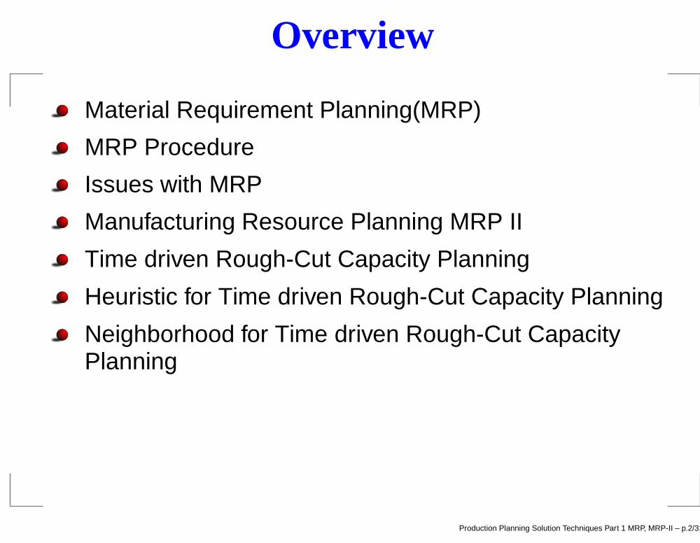
Overview
Material Requirement Planning(MRP)
MRP Procedure
Issues with MRP
Manufacturing Resource Planning MRP II
Time driven Rough-Cut Capacity Planning
Heuristic for Time driven Rough-Cut Capacity Planning
Neighborhood for Time driven Rough-Cut CapacityPlanning
Production Planning Solution Techniques Part 1 MRP, MRP-II – p.2/31
Material Requirement Planning(MRP)
Production Planning Solution Techniques Part 1 MRP, MRP-II – p.3/31

Material Requirement Planning(MRP)
Originally system was based on reorder point.
Production Planning Solution Techniques Part 1 MRP, MRP-II – p.3/31
Material Requirement Planning(MRP)
Originally system was based on reorder point.
Reorder point is suited for independent demand.
Production Planning Solution Techniques Part 1 MRP, MRP-II – p.3/31

Material Requirement Planning(MRP)
Originally system was based on reorder point.
Reorder point is suited for independent demand.
But not for dependent demand.
Production Planning Solution Techniques Part 1 MRP, MRP-II – p.3/31
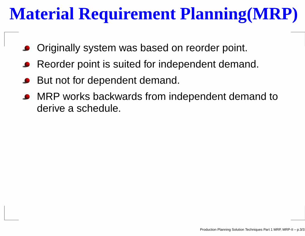
Material Requirement Planning(MRP)
Originally system was based on reorder point.
Reorder point is suited for independent demand.
But not for dependent demand.
MRP works backwards from independent demand toderive a schedule.
Production Planning Solution Techniques Part 1 MRP, MRP-II – p.3/31
Material Requirement Planning(MRP)
Originally system was based on reorder point.
Reorder point is suited for independent demand.
But not for dependent demand.
MRP works backwards from independent demand toderive a schedule.
MRP is called a push system since it pushes items inthe production chain.
Production Planning Solution Techniques Part 1 MRP, MRP-II – p.3/31

Overview of MRP
Production Planning Solution Techniques Part 1 MRP, MRP-II – p.4/31
Overview of MRP
External orders is called Purchase orders.
Production Planning Solution Techniques Part 1 MRP, MRP-II – p.4/31
Overview of MRP
External orders is called Purchase orders.
Internal orders is called Jobs.
Production Planning Solution Techniques Part 1 MRP, MRP-II – p.4/31
Overview of MRP
External orders is called Purchase orders.
Internal orders is called Jobs.
Time is divided into buckets.
Production Planning Solution Techniques Part 1 MRP, MRP-II – p.4/31
Overview of MRP
External orders is called Purchase orders.
Internal orders is called Jobs.
Time is divided into buckets.
The bill of material(BOM) describes relationship
Production Planning Solution Techniques Part 1 MRP, MRP-II – p.4/31
Overview of MRP
External orders is called Purchase orders.
Internal orders is called Jobs.
Time is divided into buckets.
The bill of material(BOM) describes relationship
The routing describes the work processes.
Production Planning Solution Techniques Part 1 MRP, MRP-II – p.4/31
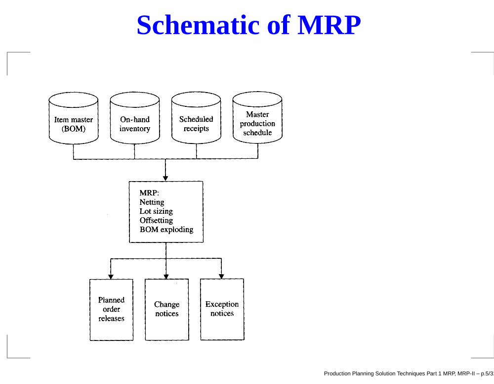
Schematic of MRP
Production Planning Solution Techniques Part 1 MRP, MRP-II – p.5/31
MRP Inputs and Outputs
Production Planning Solution Techniques Part 1 MRP, MRP-II – p.6/31

MRP Inputs and Outputs
Master Production Schedule:
Production Planning Solution Techniques Part 1 MRP, MRP-II – p.6/31
MRP Inputs and Outputs
Master Production Schedule: Item, Quantity and duedates.
Production Planning Solution Techniques Part 1 MRP, MRP-II – p.6/31
MRP Inputs and Outputs
Master Production Schedule: Item, Quantity and duedates.
Erp Database:
Production Planning Solution Techniques Part 1 MRP, MRP-II – p.6/31
MRP Inputs and Outputs
Master Production Schedule: Item, Quantity and duedates.
Erp Database: BOM, Routing, lot-sizing rule(LSR),lead time(PLT) and On-Hand Inventory.
Production Planning Solution Techniques Part 1 MRP, MRP-II – p.6/31
MRP Inputs and Outputs
Master Production Schedule: Item, Quantity and duedates.
Erp Database: BOM, Routing, lot-sizing rule(LSR),lead time(PLT) and On-Hand Inventory.
Scheduled Receipts: Out standing orders and Jobs.Work in process.
Production Planning Solution Techniques Part 1 MRP, MRP-II – p.6/31

MRP Inputs and Outputs
Master Production Schedule: Item, Quantity and duedates.
Erp Database: BOM, Routing, lot-sizing rule(LSR),lead time(PLT) and On-Hand Inventory.
Scheduled Receipts: Out standing orders and Jobs.Work in process.
MRP outputs: Planned order release, Change noticesand Exception reports.
Production Planning Solution Techniques Part 1 MRP, MRP-II – p.6/31
MRP Procedure
Production Planning Solution Techniques Part 1 MRP, MRP-II – p.7/31
MRP Procedure
T is the number of time periods.
Production Planning Solution Techniques Part 1 MRP, MRP-II – p.7/31
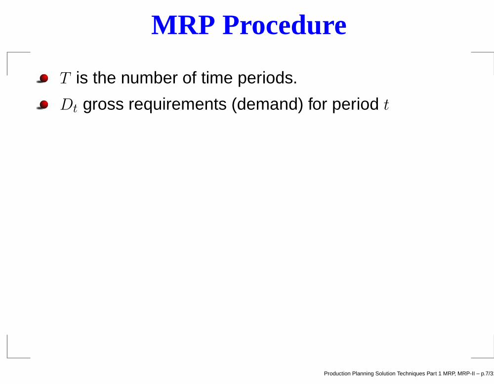
MRP Procedure
T is the number of time periods.
Dt gross requirements (demand) for period t
Production Planning Solution Techniques Part 1 MRP, MRP-II – p.7/31

MRP Procedure
T is the number of time periods.
Dt gross requirements (demand) for period t
St quantity currently scheduled to complete in period t
Production Planning Solution Techniques Part 1 MRP, MRP-II – p.7/31

MRP Procedure
T is the number of time periods.
Dt gross requirements (demand) for period t
St quantity currently scheduled to complete in period t
It Projected on-hand inventory in period t
Production Planning Solution Techniques Part 1 MRP, MRP-II – p.7/31

MRP Procedure
T is the number of time periods.
Dt gross requirements (demand) for period t
St quantity currently scheduled to complete in period t
It Projected on-hand inventory in period t
Nt net requirements for period t
Production Planning Solution Techniques Part 1 MRP, MRP-II – p.7/31
MRP Procedure: Netting
Production Planning Solution Techniques Part 1 MRP, MRP-II – p.8/31
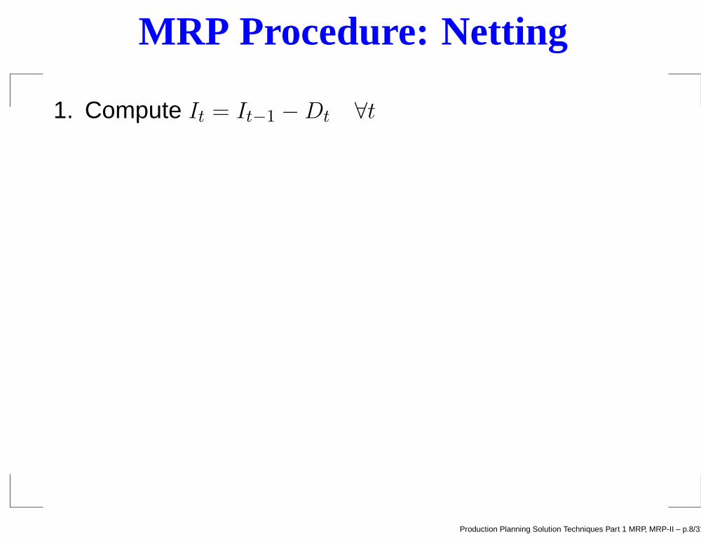
MRP Procedure: Netting
1. Compute It = It−1 − Dt ∀t
Production Planning Solution Techniques Part 1 MRP, MRP-II – p.8/31
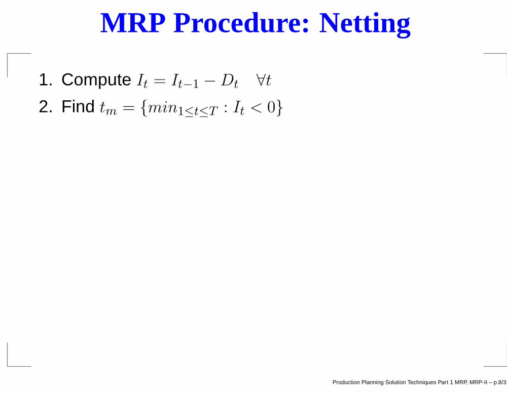
MRP Procedure: Netting
1. Compute It = It−1 − Dt ∀t
2. Find tm = {min1≤t≤T : It < 0}
Production Planning Solution Techniques Part 1 MRP, MRP-II – p.8/31
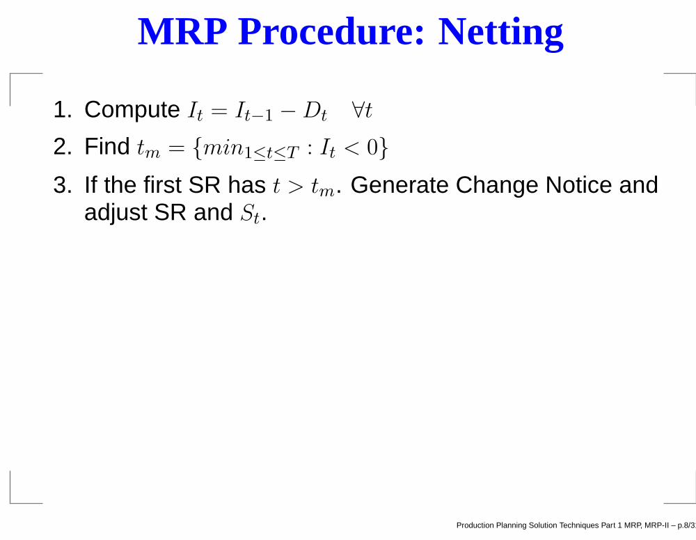
MRP Procedure: Netting
1. Compute It = It−1 − Dt ∀t
2. Find tm = {min1≤t≤T : It < 0}
3. If the first SR has t > tm. Generate Change Notice andadjust SR and St.
Production Planning Solution Techniques Part 1 MRP, MRP-II – p.8/31
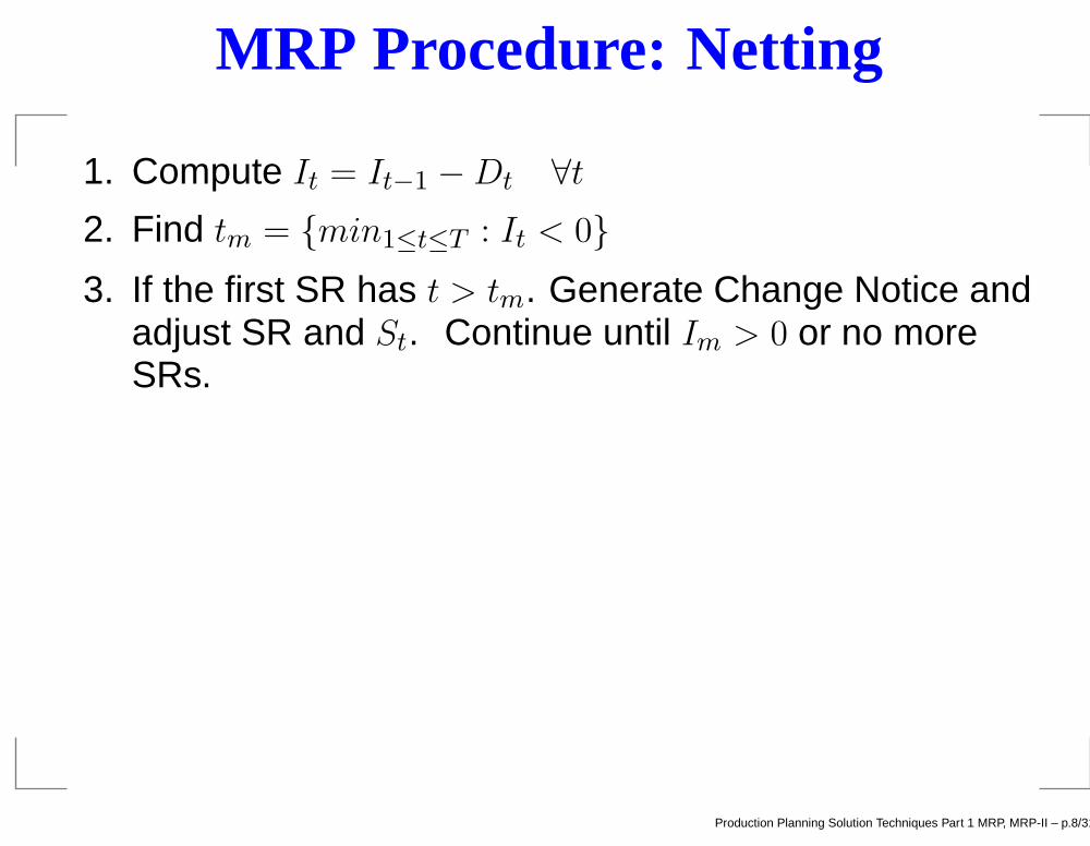
MRP Procedure: Netting
1. Compute It = It−1 − Dt ∀t
2. Find tm = {min1≤t≤T : It < 0}
3. If the first SR has t > tm. Generate Change Notice andadjust SR and St. Continue until Im > 0 or no moreSRs.
Production Planning Solution Techniques Part 1 MRP, MRP-II – p.8/31
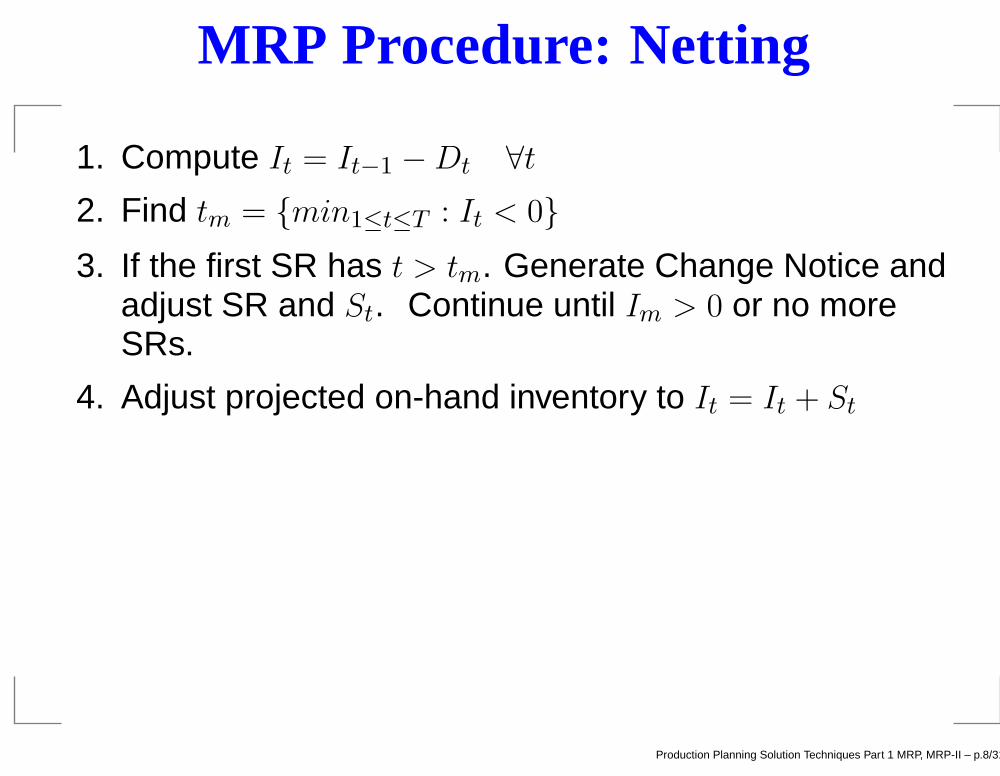
MRP Procedure: Netting
1. Compute It = It−1 − Dt ∀t
2. Find tm = {min1≤t≤T : It < 0}
3. If the first SR has t > tm. Generate Change Notice andadjust SR and St. Continue until Im > 0 or no moreSRs.
4. Adjust projected on-hand inventory to It = It + St
5. Find t∗ = {t|It < 0}
Net requirement follows as:
Nt =
0 t < t∗
−It t = t∗
Dt t > t∗
Production Planning Solution Techniques Part 1 MRP, MRP-II – p.8/31
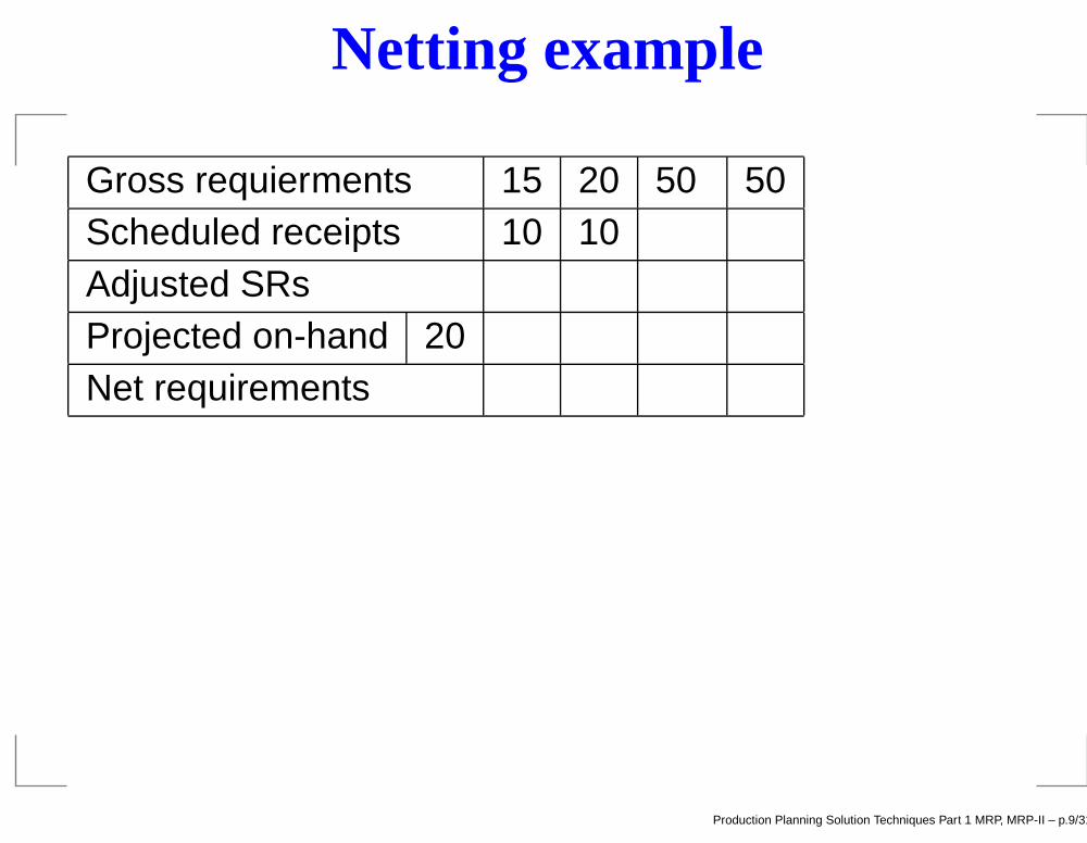
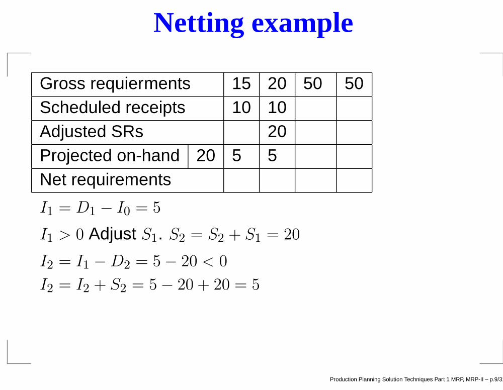
Netting example
Gross requierments 15 20 50 50Scheduled receipts 10 10Adjusted SRsProjected on-hand 20Net requirements
Production Planning Solution Techniques Part 1 MRP, MRP-II – p.9/31
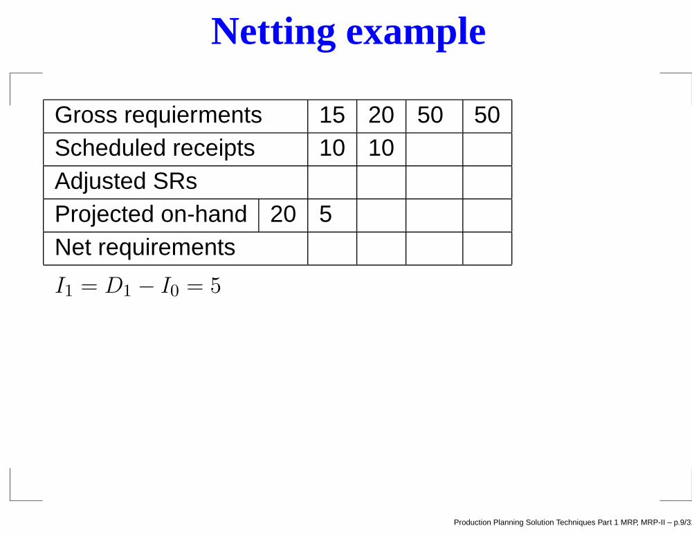
Netting example
Gross requierments 15 20 50 50Scheduled receipts 10 10Adjusted SRsProjected on-hand 20 5Net requirements
I1 = D1 − I0 = 5
Production Planning Solution Techniques Part 1 MRP, MRP-II – p.9/31
Netting example
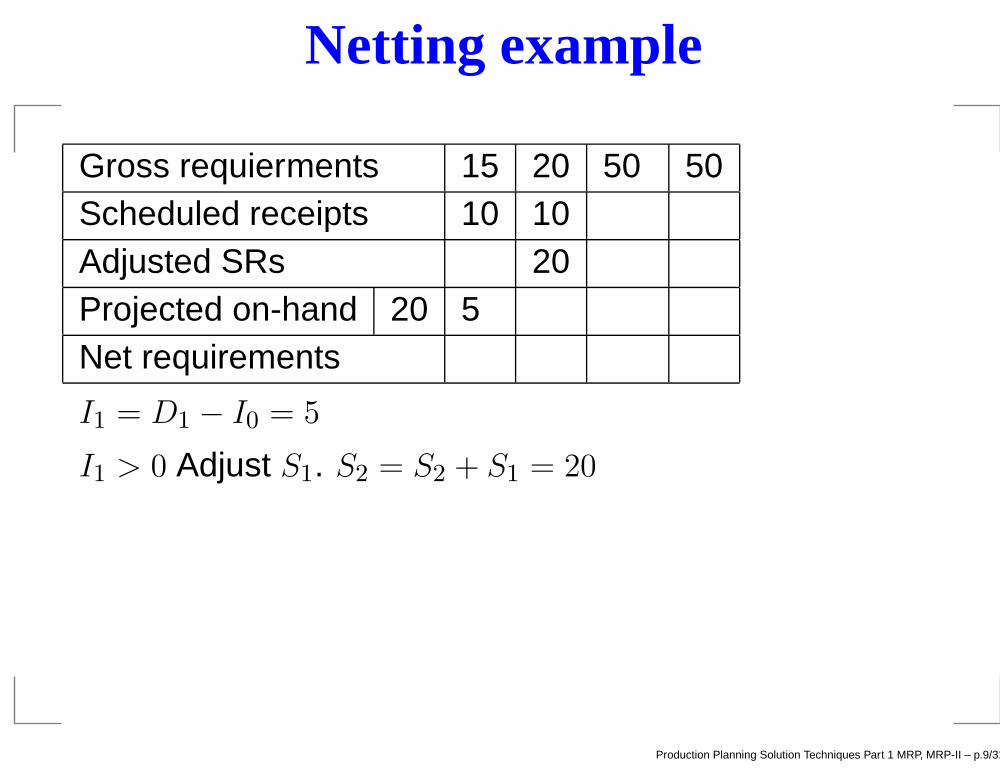
Gross requierments 15 20 50 50Scheduled receipts 10 10Adjusted SRs 20Projected on-hand 20 5Net requirements
I1 = D1 − I0 = 5
I1 > 0 Adjust S1. S2 = S2 + S1 = 20
Production Planning Solution Techniques Part 1 MRP, MRP-II – p.9/31
Netting example
Gross requierments 15 20 50 50Scheduled receipts 10 10Adjusted SRs 20Projected on-hand 20 5 5Net requirements
I1 = D1 − I0 = 5
I1 > 0 Adjust S1. S2 = S2 + S1 = 20
I2 = I1 − D2 = 5 − 20 < 0
I2 = I2 + S2 = 5 − 20 + 20 = 5
Production Planning Solution Techniques Part 1 MRP, MRP-II – p.9/31

Netting example
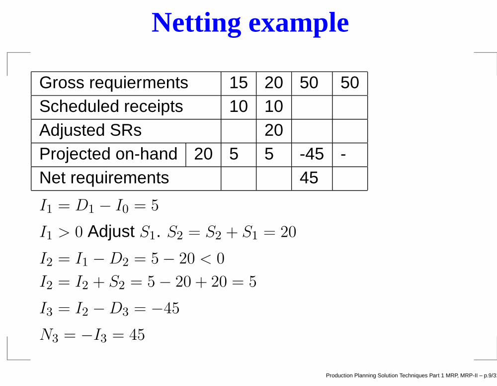
Gross requierments 15 20 50 50Scheduled receipts 10 10Adjusted SRs 20Projected on-hand 20 5 5 -45 -Net requirements
I1 = D1 − I0 = 5
I1 > 0 Adjust S1. S2 = S2 + S1 = 20
I2 = I1 − D2 = 5 − 20 < 0
I2 = I2 + S2 = 5 − 20 + 20 = 5
I3 = I2 − D3 = −45
Production Planning Solution Techniques Part 1 MRP, MRP-II – p.9/31
Netting example
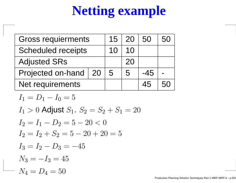
Gross requierments 15 20 50 50Scheduled receipts 10 10Adjusted SRs 20Projected on-hand 20 5 5 -45 -Net requirements 45
I1 = D1 − I0 = 5
I1 > 0 Adjust S1. S2 = S2 + S1 = 20
I2 = I1 − D2 = 5 − 20 < 0
I2 = I2 + S2 = 5 − 20 + 20 = 5
I3 = I2 − D3 = −45
N3 = −I3 = 45
Production Planning Solution Techniques Part 1 MRP, MRP-II – p.9/31
Netting example
Gross requierments 15 20 50 50Scheduled receipts 10 10Adjusted SRs 20Projected on-hand 20 5 5 -45 -Net requirements 45 50
I1 = D1 − I0 = 5
I1 > 0 Adjust S1. S2 = S2 + S1 = 20
I2 = I1 − D2 = 5 − 20 < 0
I2 = I2 + S2 = 5 − 20 + 20 = 5
I3 = I2 − D3 = −45
N3 = −I3 = 45
N4 = D4 = 50Production Planning Solution Techniques Part 1 MRP, MRP-II – p.9/31
MRP Procedure continued
Production Planning Solution Techniques Part 1 MRP, MRP-II – p.10/31
MRP Procedure continued
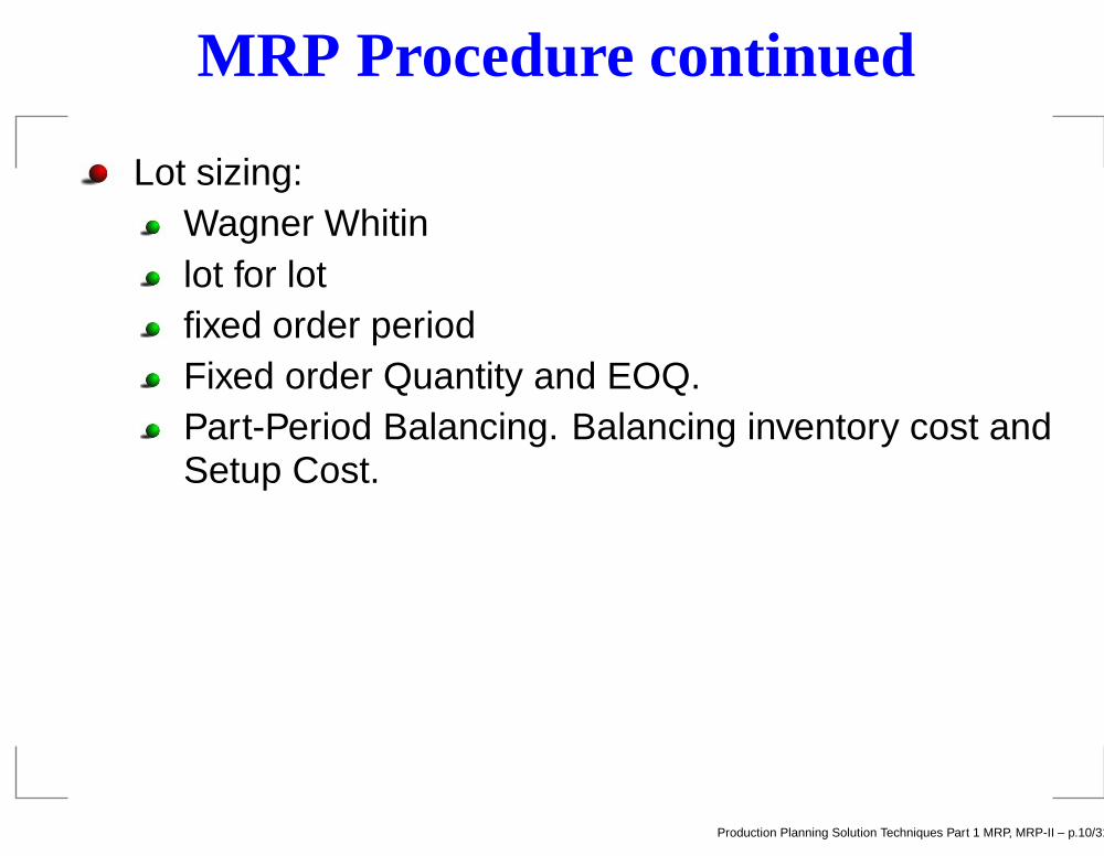
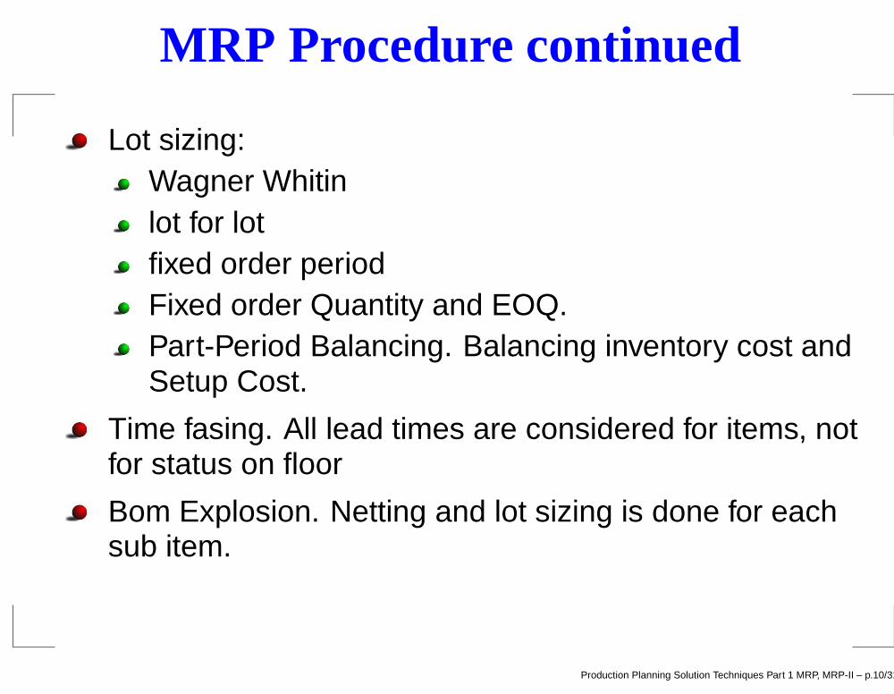
Lot sizing:
Production Planning Solution Techniques Part 1 MRP, MRP-II – p.10/31

MRP Procedure continued
Lot sizing:Wagner Whitin
Production Planning Solution Techniques Part 1 MRP, MRP-II – p.10/31
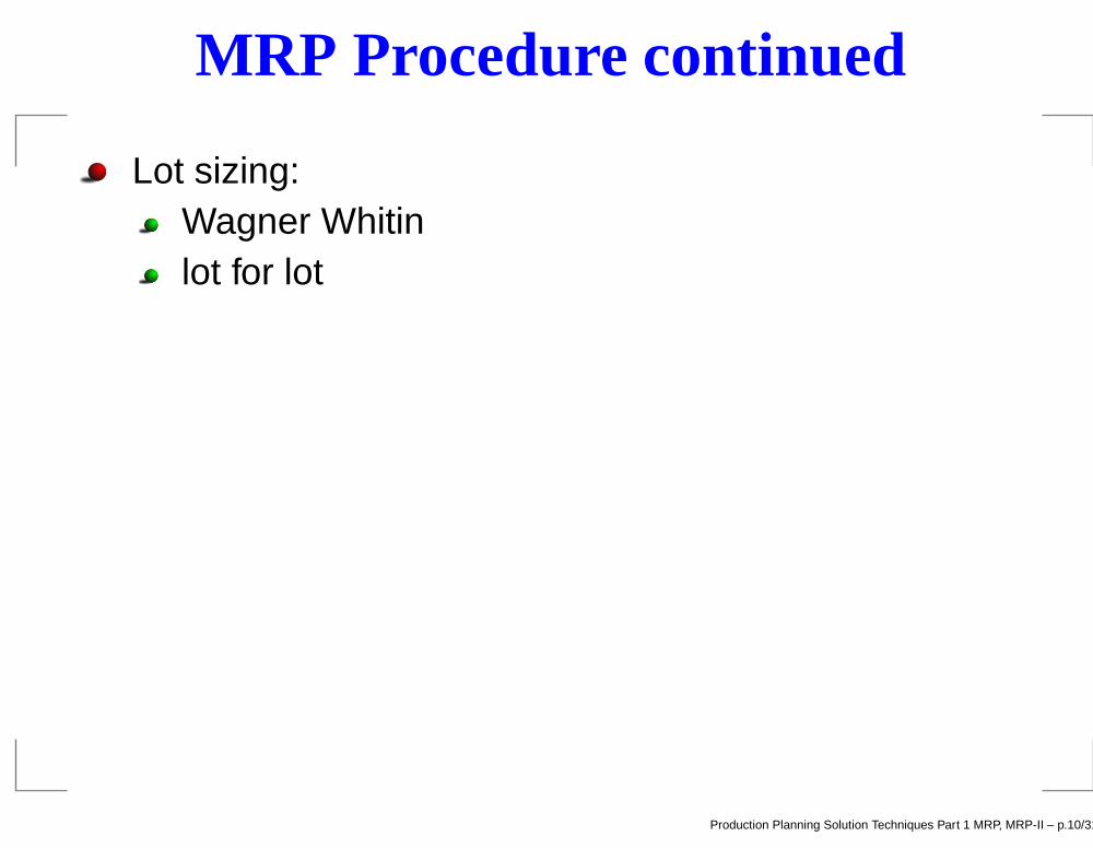
MRP Procedure continued
Lot sizing:Wagner Whitinlot for lot
Production Planning Solution Techniques Part 1 MRP, MRP-II – p.10/31
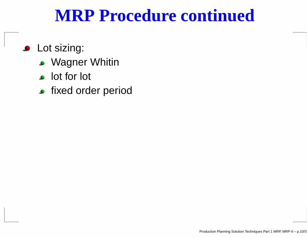
MRP Procedure continued
Lot sizing:Wagner Whitinlot for lotfixed order period
Production Planning Solution Techniques Part 1 MRP, MRP-II – p.10/31
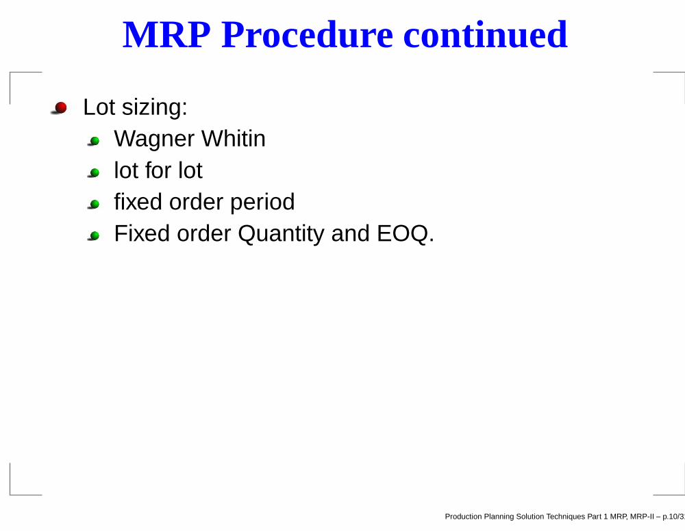
MRP Procedure continued
Lot sizing:Wagner Whitinlot for lotfixed order periodFixed order Quantity and EOQ.
Production Planning Solution Techniques Part 1 MRP, MRP-II – p.10/31
MRP Procedure continued
Lot sizing:Wagner Whitinlot for lotfixed order periodFixed order Quantity and EOQ.Part-Period Balancing. Balancing inventory cost andSetup Cost.
Production Planning Solution Techniques Part 1 MRP, MRP-II – p.10/31

MRP Procedure continued
Lot sizing:Wagner Whitinlot for lotfixed order periodFixed order Quantity and EOQ.Part-Period Balancing. Balancing inventory cost andSetup Cost.
Time fasing. All lead times are considered for items, notfor status on floor
Production Planning Solution Techniques Part 1 MRP, MRP-II – p.10/31
MRP Procedure continued
Lot sizing:Wagner Whitinlot for lotfixed order periodFixed order Quantity and EOQ.Part-Period Balancing. Balancing inventory cost andSetup Cost.
Time fasing. All lead times are considered for items, notfor status on floor
Bom Explosion. Netting and lot sizing is done for eachsub item.
Production Planning Solution Techniques Part 1 MRP, MRP-II – p.10/31
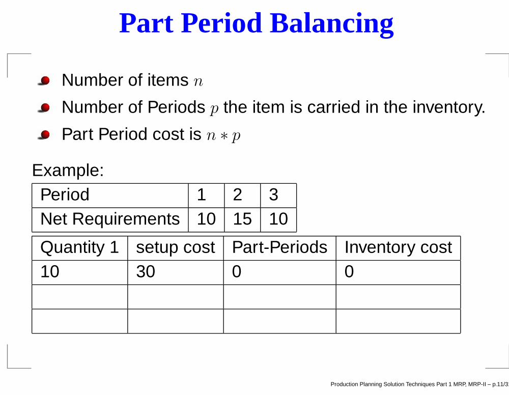
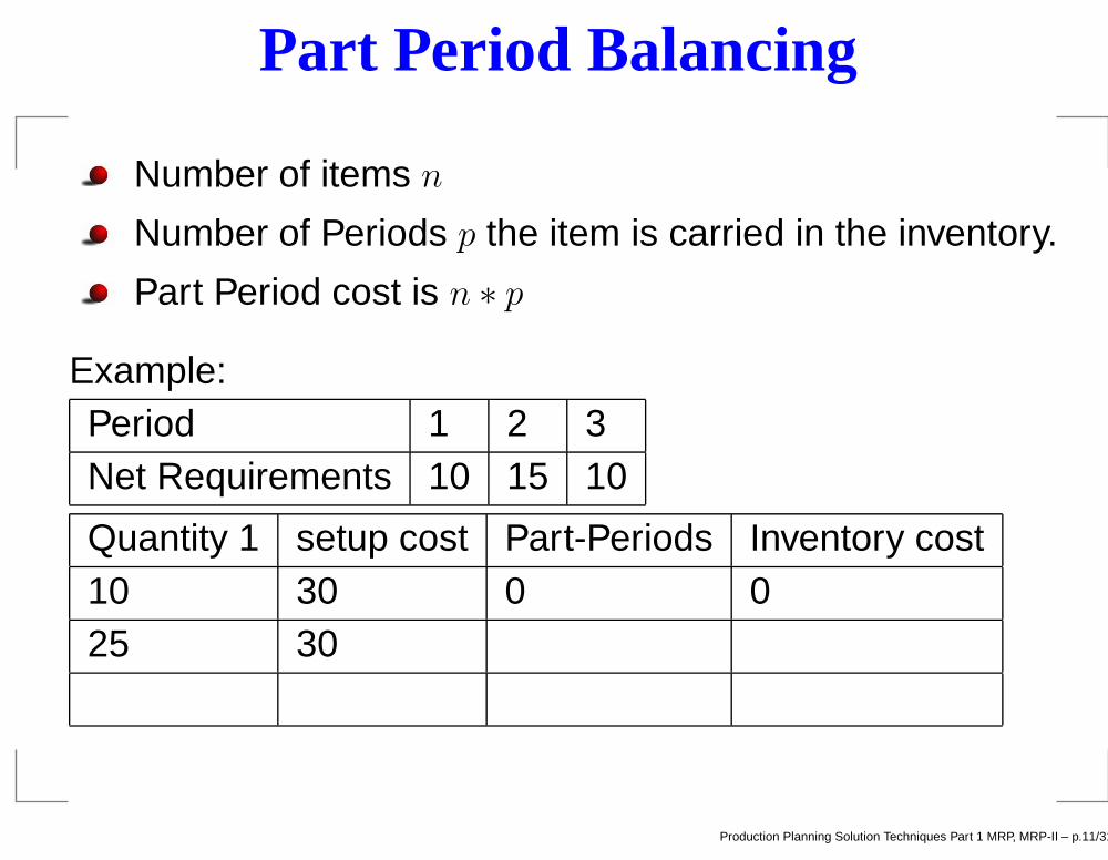
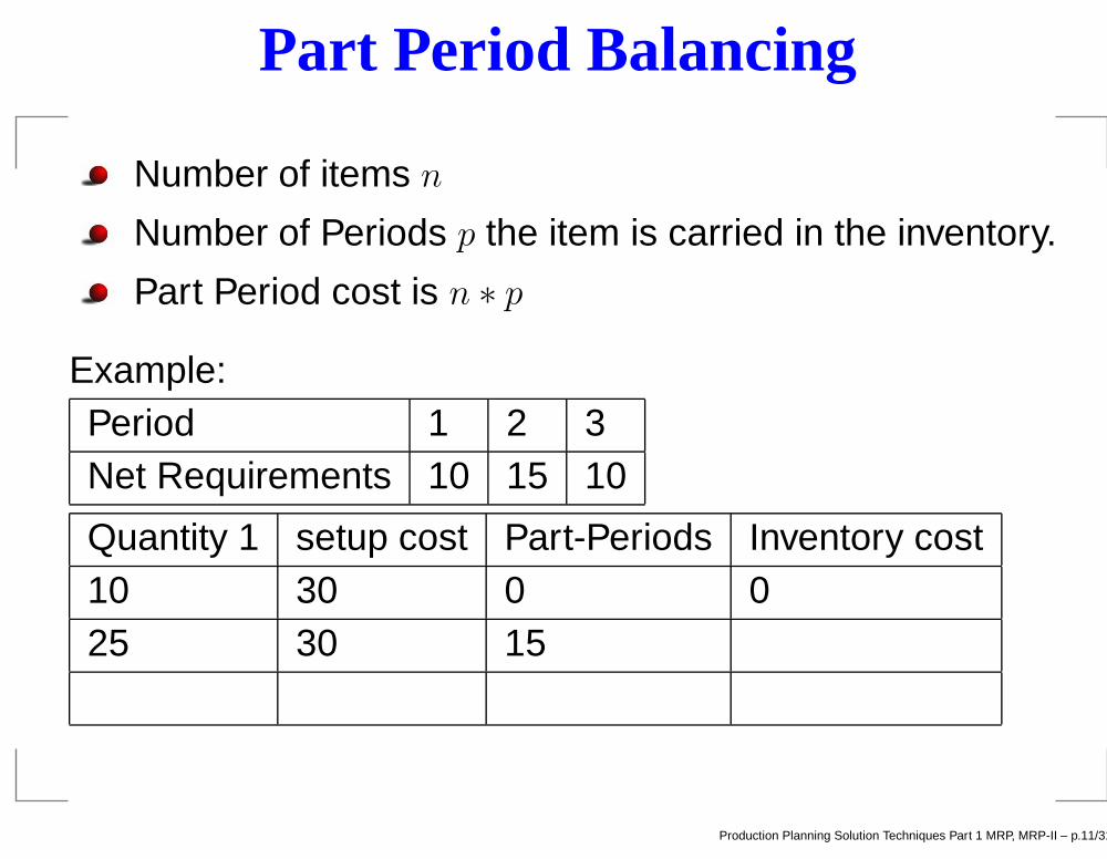
Part Period Balancing
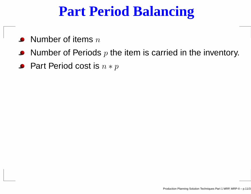
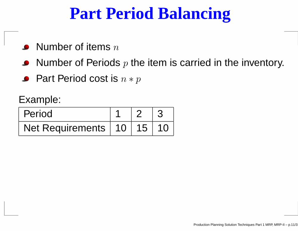
Number of items n
Number of Periods p the item is carried in the inventory.
Part Period cost is n ∗ p
Production Planning Solution Techniques Part 1 MRP, MRP-II – p.11/31
Part Period Balancing
Number of items n
Number of Periods p the item is carried in the inventory.
Part Period cost is n ∗ p
Example:Period 1 2 3Net Requirements 10 15 10
Production Planning Solution Techniques Part 1 MRP, MRP-II – p.11/31
Part Period Balancing
Number of items n
Number of Periods p the item is carried in the inventory.
Part Period cost is n ∗ p
Example:Period 1 2 3Net Requirements 10 15 10
Quantity 1 setup cost Part-Periods Inventory cost10 30 0 0
Production Planning Solution Techniques Part 1 MRP, MRP-II – p.11/31

Part Period Balancing
Number of items n
Number of Periods p the item is carried in the inventory.
Part Period cost is n ∗ p
Example:Period 1 2 3Net Requirements 10 15 10
Quantity 1 setup cost Part-Periods Inventory cost10 30 0 025
Production Planning Solution Techniques Part 1 MRP, MRP-II – p.11/31
Part Period Balancing
Number of items n
Number of Periods p the item is carried in the inventory.
Part Period cost is n ∗ p
Example:Period 1 2 3Net Requirements 10 15 10
Quantity 1 setup cost Part-Periods Inventory cost10 30 0 025 30
Production Planning Solution Techniques Part 1 MRP, MRP-II – p.11/31
Part Period Balancing
Number of items n
Number of Periods p the item is carried in the inventory.
Part Period cost is n ∗ p
Example:Period 1 2 3Net Requirements 10 15 10
Quantity 1 setup cost Part-Periods Inventory cost10 30 0 025 30 15
Production Planning Solution Techniques Part 1 MRP, MRP-II – p.11/31

Part Period Balancing
Number of items n
Number of Periods p the item is carried in the inventory.
Part Period cost is n ∗ p
Example:Period 1 2 3Net Requirements 10 15 10
Quantity 1 setup cost Part-Periods Inventory cost10 30 0 025 30 15 15
Production Planning Solution Techniques Part 1 MRP, MRP-II – p.11/31

Part Period Balancing
Number of items n
Number of Periods p the item is carried in the inventory.
Part Period cost is n ∗ p
Example:Period 1 2 3Net Requirements 10 15 10
Quantity 1 setup cost Part-Periods Inventory cost10 30 0 025 30 15 1535
Production Planning Solution Techniques Part 1 MRP, MRP-II – p.11/31

Part Period Balancing
Number of items n
Number of Periods p the item is carried in the inventory.
Part Period cost is n ∗ p
Example:Period 1 2 3Net Requirements 10 15 10
Quantity 1 setup cost Part-Periods Inventory cost10 30 0 025 30 15 1535 30
Production Planning Solution Techniques Part 1 MRP, MRP-II – p.11/31

Part Period Balancing
Number of items n
Number of Periods p the item is carried in the inventory.
Part Period cost is n ∗ p
Example:Period 1 2 3Net Requirements 10 15 10
Quantity 1 setup cost Part-Periods Inventory cost10 30 0 025 30 15 1535 30 35
Production Planning Solution Techniques Part 1 MRP, MRP-II – p.11/31

Part Period Balancing
Number of items n
Number of Periods p the item is carried in the inventory.
Part Period cost is n ∗ p
Example:Period 1 2 3Net Requirements 10 15 10
Quantity 1 setup cost Part-Periods Inventory cost10 30 0 025 30 15 1535 30 35 35
Production Planning Solution Techniques Part 1 MRP, MRP-II – p.11/31
Issues with MRP
Production Planning Solution Techniques Part 1 MRP, MRP-II – p.12/31
Issues with MRP
Assume constant lead times. To take care of variationSafety Stock and Safety Lead time is used.
Production Planning Solution Techniques Part 1 MRP, MRP-II – p.12/31

Issues with MRP
Assume constant lead times. To take care of variationSafety Stock and Safety Lead time is used.
Capacity Infeasibility, there is no capacity check.
Production Planning Solution Techniques Part 1 MRP, MRP-II – p.12/31

Issues with MRP
Assume constant lead times. To take care of variationSafety Stock and Safety Lead time is used.
Capacity Infeasibility, there is no capacity check.
Long Planned Lead time due to variation in deliverytime.
Production Planning Solution Techniques Part 1 MRP, MRP-II – p.12/31

Issues with MRP
Assume constant lead times. To take care of variationSafety Stock and Safety Lead time is used.
Capacity Infeasibility, there is no capacity check.
Long Planned Lead time due to variation in deliverytime.
System Nervousness. Plans that are feasible canbecome infeasible.
Production Planning Solution Techniques Part 1 MRP, MRP-II – p.12/31

Questians or comments to MRP
Are there any questians or comments ?
Production Planning Solution Techniques Part 1 MRP, MRP-II – p.13/31

Manufacturing Resource Planning
Production Planning Solution Techniques Part 1 MRP, MRP-II – p.14/31
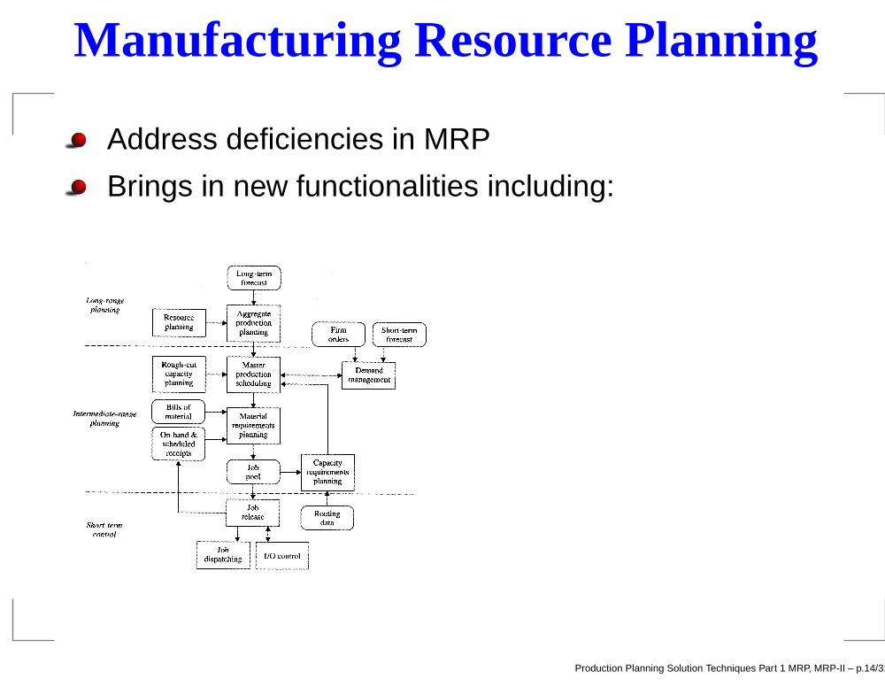
Manufacturing Resource Planning
Address deficiencies in MRP
Production Planning Solution Techniques Part 1 MRP, MRP-II – p.14/31

Manufacturing Resource Planning
Address deficiencies in MRP
Brings in new functionalities including:
Production Planning Solution Techniques Part 1 MRP, MRP-II – p.14/31
Manufacturing Resource Planning
Address deficiencies in MRP
Brings in new functionalities including:
Production Planning Solution Techniques Part 1 MRP, MRP-II – p.14/31
Long-Range Planning
Production Planning Solution Techniques Part 1 MRP, MRP-II – p.15/31
Long-Range Planning
Forecasting seeks to predict demands of the future.
Production Planning Solution Techniques Part 1 MRP, MRP-II – p.15/31

Long-Range Planning
Forecasting seeks to predict demands of the future.
Resource Planning. Determines long time capacityneed. Is used to decide is knew facilities must be buildor old facilities must be expanded.
Production Planning Solution Techniques Part 1 MRP, MRP-II – p.15/31
Long-Range Planning
Forecasting seeks to predict demands of the future.
Resource Planning. Determines long time capacityneed. Is used to decide is knew facilities must be buildor old facilities must be expanded.
Aggregate Planning. Determines how inventory is build.Do we use overtime or do we carry inventory over along period.
Production Planning Solution Techniques Part 1 MRP, MRP-II – p.15/31
Intermidiate Planning
Production Planning Solution Techniques Part 1 MRP, MRP-II – p.16/31
Intermidiate Planning
Demand management Converts long-term forecast intoactual customer orders and forecast of anticipatedorders.
Production Planning Solution Techniques Part 1 MRP, MRP-II – p.16/31

Intermidiate Planning
Demand management Converts long-term forecast intoactual customer orders and forecast of anticipatedorders.
Available to promise Secures that an order can be meetat a given due date. This can be done by using forwardloading.
Master Production Schedule Generates an anticipatedproduction schedule.
Production Planning Solution Techniques Part 1 MRP, MRP-II – p.16/31
Intermidiate Planning
Demand management Converts long-term forecast intoactual customer orders and forecast of anticipatedorders.
Available to promise Secures that an order can be meetat a given due date. This can be done by using forwardloading.
Master Production Schedule Generates an anticipatedproduction schedule.
Rough-cut Planning Provides a schedule where thecapacity on critical resources is meet.
Production Planning Solution Techniques Part 1 MRP, MRP-II – p.16/31

Intermidiate Planning
Demand management Converts long-term forecast intoactual customer orders and forecast of anticipatedorders.
Available to promise Secures that an order can be meetat a given due date. This can be done by using forwardloading.
Master Production Schedule Generates an anticipatedproduction schedule.
Rough-cut Planning Provides a schedule where thecapacity on critical resources is meet.
Capacity Requirements Planning Does not preformactual capacity check. CRP assumes infinite capacityon resources. Basically it just calculates finish datesbased on fixed lead times.
Production Planning Solution Techniques Part 1 MRP, MRP-II – p.16/31

Short-term control
Production Planning Solution Techniques Part 1 MRP, MRP-II – p.17/31
Short-term control
Job release Converts jobs to scheduled receipts.Resolves conflicts if several high-level items uses samelow-level item.
Production Planning Solution Techniques Part 1 MRP, MRP-II – p.17/31

Short-term control
Job release Converts jobs to scheduled receipts.Resolves conflicts if several high-level items uses samelow-level item.
Job dispatching Maintains queue in front of eachworkstation and try to maintain due date.
Production Planning Solution Techniques Part 1 MRP, MRP-II – p.17/31
Short-term control
Job release Converts jobs to scheduled receipts.Resolves conflicts if several high-level items uses samelow-level item.
Job dispatching Maintains queue in front of eachworkstation and try to maintain due date.
Shortest process time Chooses the shortest job
Production Planning Solution Techniques Part 1 MRP, MRP-II – p.17/31
Short-term control
Job release Converts jobs to scheduled receipts.Resolves conflicts if several high-level items uses samelow-level item.
Job dispatching Maintains queue in front of eachworkstation and try to maintain due date.
Shortest process time Chooses the shortest jobEarliest due date dispatches job with nearest duedate
Production Planning Solution Techniques Part 1 MRP, MRP-II – p.17/31
Short-term control
Job release Converts jobs to scheduled receipts.Resolves conflicts if several high-level items uses samelow-level item.
Job dispatching Maintains queue in front of eachworkstation and try to maintain due date.
Shortest process time Chooses the shortest jobEarliest due date dispatches job with nearest duedateLeast slack Choose job where, the due date minusremaining process time is lowest.
Production Planning Solution Techniques Part 1 MRP, MRP-II – p.17/31
Short-term control
Job release Converts jobs to scheduled receipts.Resolves conflicts if several high-level items uses samelow-level item.
Job dispatching Maintains queue in front of eachworkstation and try to maintain due date.
Shortest process time Chooses the shortest jobEarliest due date dispatches job with nearest duedateLeast slack Choose job where, the due date minusremaining process time is lowest.Least slack per remaining operation Divide slackwith number of operation remaining on routing.
Production Planning Solution Techniques Part 1 MRP, MRP-II – p.17/31

Questians or comments to MRP II
Are there any questians or comments ?
Production Planning Solution Techniques Part 1 MRP, MRP-II – p.18/31

Rough-Cut Capacity Planning(RCCP)
Production Planning Solution Techniques Part 1 MRP, MRP-II – p.19/31
Rough-Cut Capacity Planning(RCCP)
Considers aggregated work
Production Planning Solution Techniques Part 1 MRP, MRP-II – p.19/31
Rough-Cut Capacity Planning(RCCP)
Considers aggregated work
Allocates work in time buckets
Production Planning Solution Techniques Part 1 MRP, MRP-II – p.19/31
Rough-Cut Capacity Planning(RCCP)
Considers aggregated work
Allocates work in time buckets
Determines resources in order to reach due dates
Production Planning Solution Techniques Part 1 MRP, MRP-II – p.19/31
Rough-Cut Capacity Planning(RCCP)
Considers aggregated work
Allocates work in time buckets
Determines resources in order to reach due dates
Both regular and nonregular (outsourcing over timeetc.) is considered
Production Planning Solution Techniques Part 1 MRP, MRP-II – p.19/31
Rough-Cut Capacity Planning(RCCP)
Considers aggregated work
Allocates work in time buckets
Determines resources in order to reach due dates
Both regular and nonregular (outsourcing over timeetc.) is considered
Time driven RCCP is when project dates must be meet.
In resource-driven RCCP only regular capacity can beused
Production Planning Solution Techniques Part 1 MRP, MRP-II – p.19/31

Rough-Cut Capacity Planning(RCCP)
Considers aggregated work
Allocates work in time buckets
Determines resources in order to reach due dates
Both regular and nonregular (outsourcing over timeetc.) is considered
Time driven RCCP is when project dates must be meet.
In resource-driven RCCP only regular capacity can beused
This session will consider the time driven
Production Planning Solution Techniques Part 1 MRP, MRP-II – p.19/31
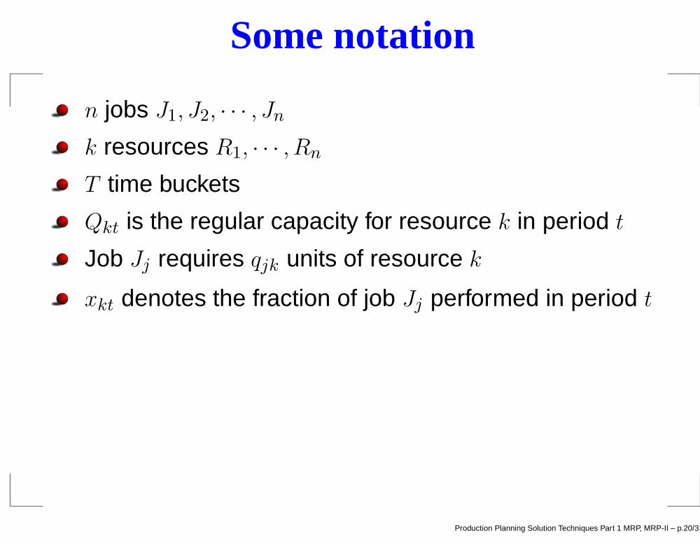
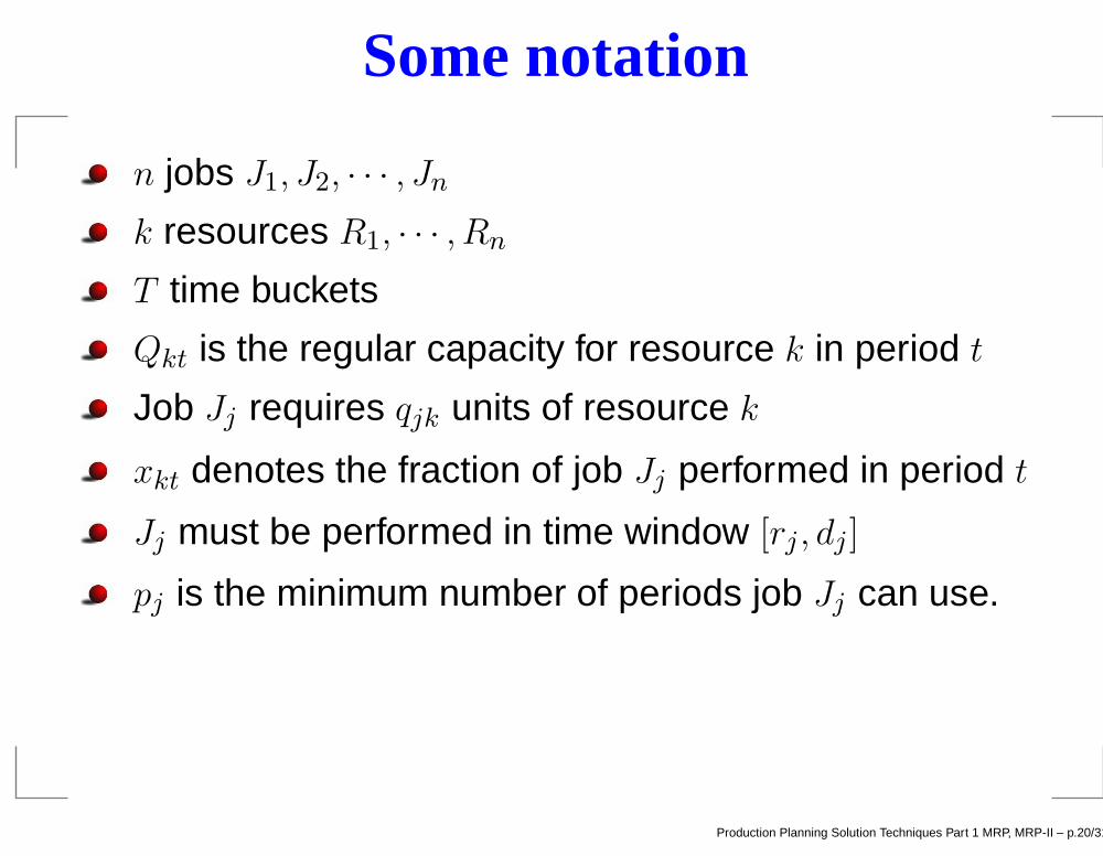
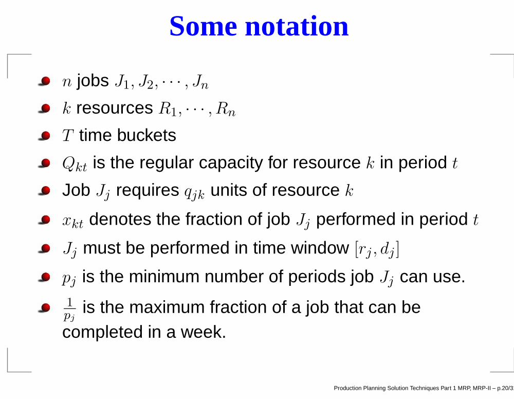
Some notation
Production Planning Solution Techniques Part 1 MRP, MRP-II – p.20/31
Some notation
n jobs J1, J2, · · · , Jn
Production Planning Solution Techniques Part 1 MRP, MRP-II – p.20/31

Some notation
n jobs J1, J2, · · · , Jn
k resources R1, · · · , Rn
Production Planning Solution Techniques Part 1 MRP, MRP-II – p.20/31
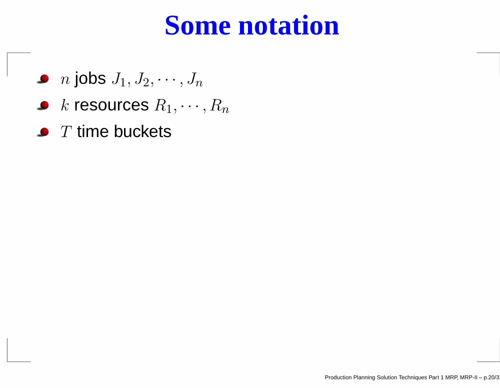
Some notation
n jobs J1, J2, · · · , Jn
k resources R1, · · · , Rn
T time buckets
Production Planning Solution Techniques Part 1 MRP, MRP-II – p.20/31
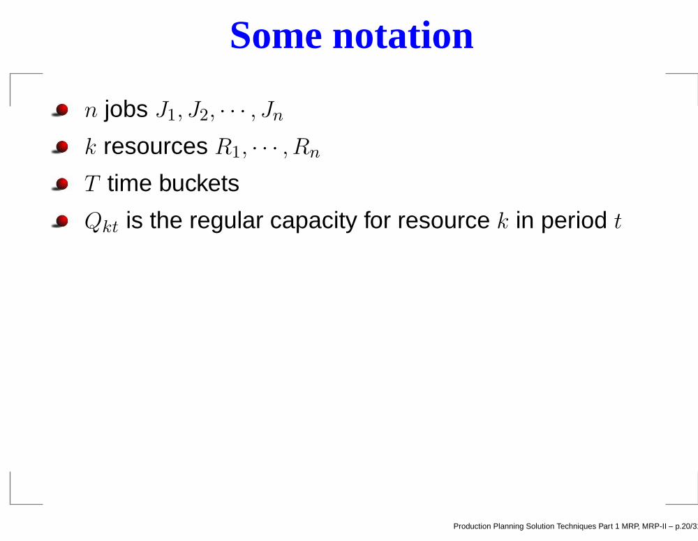
Some notation
n jobs J1, J2, · · · , Jn
k resources R1, · · · , Rn
T time buckets
Qkt is the regular capacity for resource k in period t
Production Planning Solution Techniques Part 1 MRP, MRP-II – p.20/31

Some notation
n jobs J1, J2, · · · , Jn
k resources R1, · · · , Rn
T time buckets
Qkt is the regular capacity for resource k in period t
Job Jj requires qjk units of resource k
Production Planning Solution Techniques Part 1 MRP, MRP-II – p.20/31
Some notation
n jobs J1, J2, · · · , Jn
k resources R1, · · · , Rn
T time buckets
Qkt is the regular capacity for resource k in period t
Job Jj requires qjk units of resource k
xkt denotes the fraction of job Jj performed in period t
Production Planning Solution Techniques Part 1 MRP, MRP-II – p.20/31

Some notation
n jobs J1, J2, · · · , Jn
k resources R1, · · · , Rn
T time buckets
Qkt is the regular capacity for resource k in period t
Job Jj requires qjk units of resource k
xkt denotes the fraction of job Jj performed in period t
Jj must be performed in time window [rj , dj ]
Production Planning Solution Techniques Part 1 MRP, MRP-II – p.20/31
Some notation
n jobs J1, J2, · · · , Jn
k resources R1, · · · , Rn
T time buckets
Qkt is the regular capacity for resource k in period t
Job Jj requires qjk units of resource k
xkt denotes the fraction of job Jj performed in period t
Jj must be performed in time window [rj , dj ]
pj is the minimum number of periods job Jj can use.
Production Planning Solution Techniques Part 1 MRP, MRP-II – p.20/31
Some notation
n jobs J1, J2, · · · , Jn
k resources R1, · · · , Rn
T time buckets
Qkt is the regular capacity for resource k in period t
Job Jj requires qjk units of resource k
xkt denotes the fraction of job Jj performed in period t
Jj must be performed in time window [rj , dj ]
pj is the minimum number of periods job Jj can use.1
pjis the maximum fraction of a job that can be
completed in a week.
Production Planning Solution Techniques Part 1 MRP, MRP-II – p.20/31
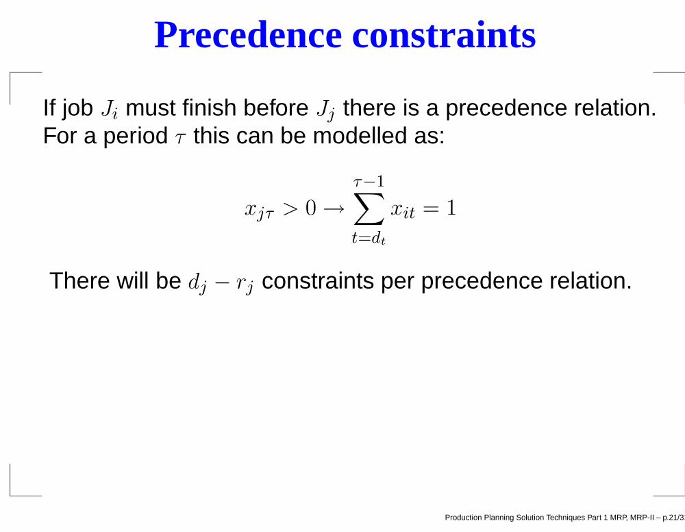
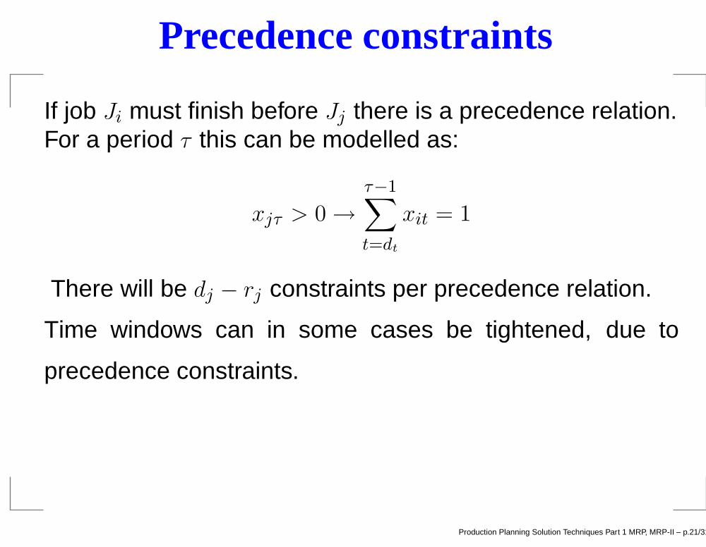
Precedence constraints
If job Ji must finish before Jj there is a precedence relation.For a period τ this can be modelled as:
Production Planning Solution Techniques Part 1 MRP, MRP-II – p.21/31

Precedence constraints
If job Ji must finish before Jj there is a precedence relation.For a period τ this can be modelled as:
xjτ > 0 →τ−1∑
t=dt
xit = 1
Production Planning Solution Techniques Part 1 MRP, MRP-II – p.21/31
Precedence constraints
If job Ji must finish before Jj there is a precedence relation.For a period τ this can be modelled as:
xjτ > 0 →τ−1∑
t=dt
xit = 1
There will be dj − rj constraints per precedence relation.
Production Planning Solution Techniques Part 1 MRP, MRP-II – p.21/31
Precedence constraints
If job Ji must finish before Jj there is a precedence relation.For a period τ this can be modelled as:
xjτ > 0 →τ−1∑
t=dt
xit = 1
There will be dj − rj constraints per precedence relation.
Time windows can in some cases be tightened, due to
precedence constraints.
Production Planning Solution Techniques Part 1 MRP, MRP-II – p.21/31
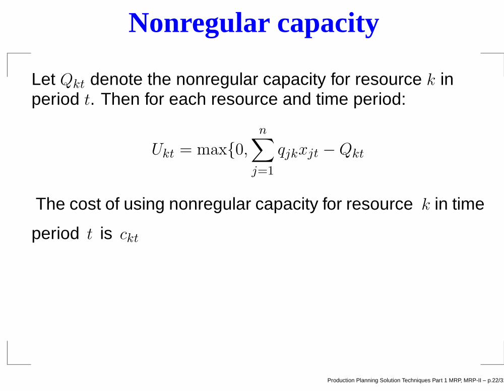
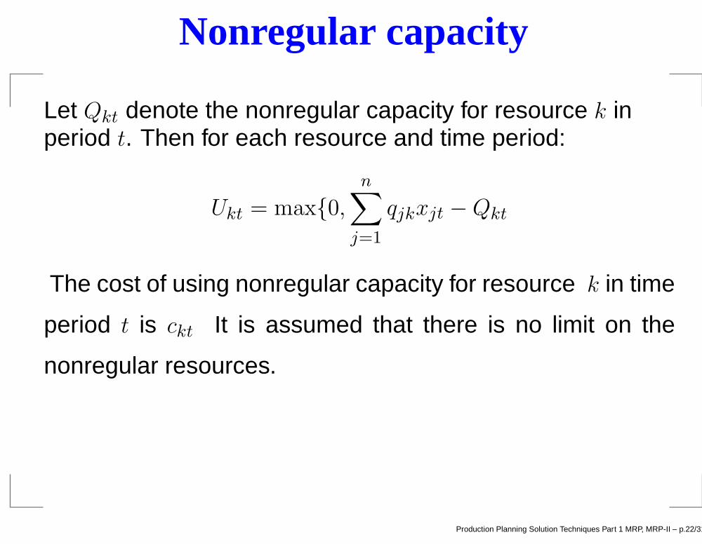
Nonregular capacity
Let Qkt denote the nonregular capacity for resource k inperiod t. Then for each resource and time period:
Production Planning Solution Techniques Part 1 MRP, MRP-II – p.22/31
Nonregular capacity
Let Qkt denote the nonregular capacity for resource k inperiod t. Then for each resource and time period:
Ukt = max{0,n
∑
j=1
qjkxjt − Qkt
Production Planning Solution Techniques Part 1 MRP, MRP-II – p.22/31
Nonregular capacity
Let Qkt denote the nonregular capacity for resource k inperiod t. Then for each resource and time period:
Ukt = max{0,n
∑
j=1
qjkxjt − Qkt
The cost of using nonregular capacity for resource k in time
period t is ckt
Production Planning Solution Techniques Part 1 MRP, MRP-II – p.22/31
Nonregular capacity
Let Qkt denote the nonregular capacity for resource k inperiod t. Then for each resource and time period:
Ukt = max{0,n
∑
j=1
qjkxjt − Qkt
The cost of using nonregular capacity for resource k in time
period t is ckt It is assumed that there is no limit on the
nonregular resources.
Production Planning Solution Techniques Part 1 MRP, MRP-II – p.22/31
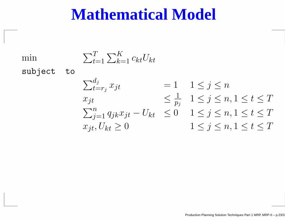
Mathematical Model
min∑T
t=1
∑Kk=1
cktUkt
subject to∑dj
t=rjxjt = 1 1 ≤ j ≤ n
xjt ≤ 1
pj1 ≤ j ≤ n, 1 ≤ t ≤ T
∑nj=1
qjkxjt − Ukt ≤ 0 1 ≤ j ≤ n, 1 ≤ t ≤ T
xjt, Ukt ≥ 0 1 ≤ j ≤ n, 1 ≤ t ≤ T
Production Planning Solution Techniques Part 1 MRP, MRP-II – p.23/31

Controlling feasibility
Allowed To Work window for job Jj is defined as [Sj , Cj ].
Production Planning Solution Techniques Part 1 MRP, MRP-II – p.24/31

Controlling feasibility
Allowed To Work window for job Jj is defined as [Sj , Cj ].
Job Jj cannot start before Sj or after Cj
Production Planning Solution Techniques Part 1 MRP, MRP-II – p.24/31
Controlling feasibility
Allowed To Work window for job Jj is defined as [Sj , Cj ].
Job Jj cannot start before Sj or after Cj
A ATW for job Jj is feasible if:
Production Planning Solution Techniques Part 1 MRP, MRP-II – p.24/31
Controlling feasibility
Allowed To Work window for job Jj is defined as [Sj , Cj ].
Job Jj cannot start before Sj or after Cj
A ATW for job Jj is feasible if:
1. Sj ≥ rj and Cj ≤ dj
2. Cj − Sj ≥ pj − 1
Production Planning Solution Techniques Part 1 MRP, MRP-II – p.24/31
Controlling feasibility
Allowed To Work window for job Jj is defined as [Sj , Cj ].
Job Jj cannot start before Sj or after Cj
A ATW for job Jj is feasible if:
1. Sj ≥ rj and Cj ≤ dj
2. Cj − Sj ≥ pj − 1
A set S of ATW windows is feasible if:
Production Planning Solution Techniques Part 1 MRP, MRP-II – p.24/31

Controlling feasibility
Allowed To Work window for job Jj is defined as [Sj , Cj ].
Job Jj cannot start before Sj or after Cj
A ATW for job Jj is feasible if:
1. Sj ≥ rj and Cj ≤ dj
2. Cj − Sj ≥ pj − 1
A set S of ATW windows is feasible if:
1. Every ATW window is feasible
2. Sj > Cj if Ji → Jj
Production Planning Solution Techniques Part 1 MRP, MRP-II – p.24/31

Mathematical Model ATW windows
sjt =
{
1 Sj ≤ t ≤ Cj
0 otherwise
(PS) min∑T
t=1
∑Kk=1
cktUkt
subjectto∑dj
t=rjxjt = 1 1 ≤ j ≤ n
xjt ≤ sj
pj1 ≤ j ≤ n, 1 ≤ t ≤ T
∑nj=1
qjkxjt − Ukt ≤ 0 1 ≤ j ≤ n, 1 ≤ t ≤ T
xjt, Ukt ≥ 0 1 ≤ j ≤ n, 1 ≤ t ≤ T
Production Planning Solution Techniques Part 1 MRP, MRP-II – p.25/31
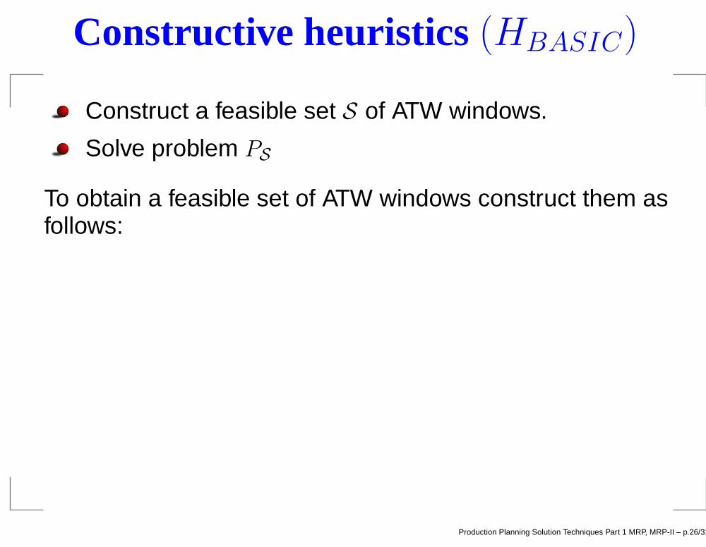
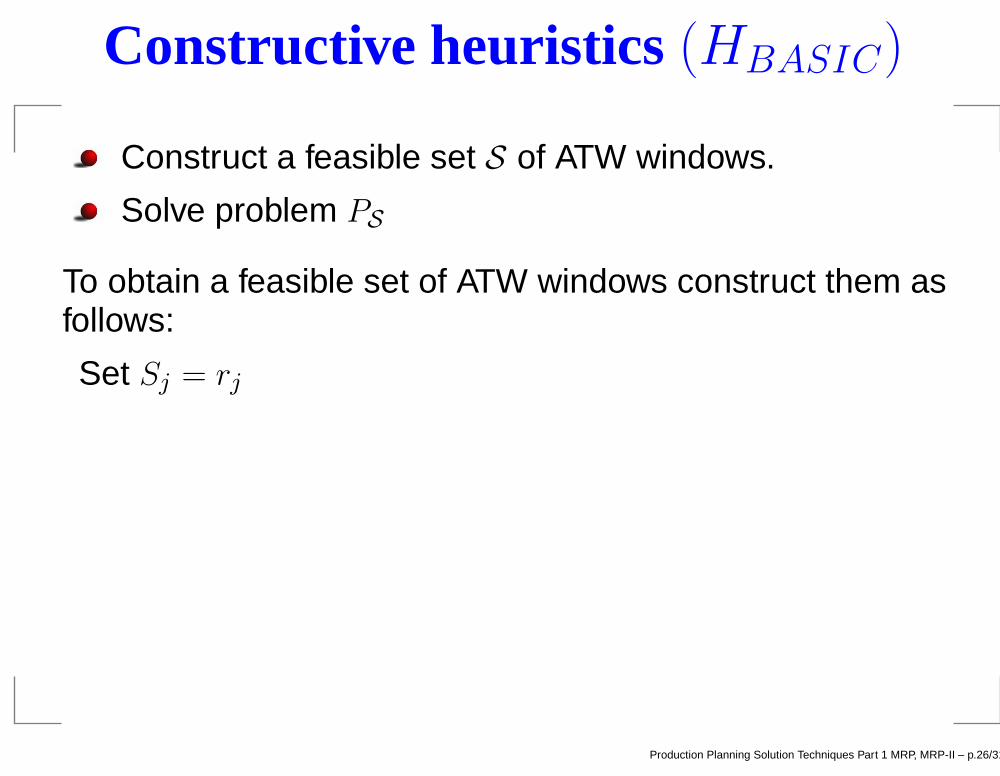
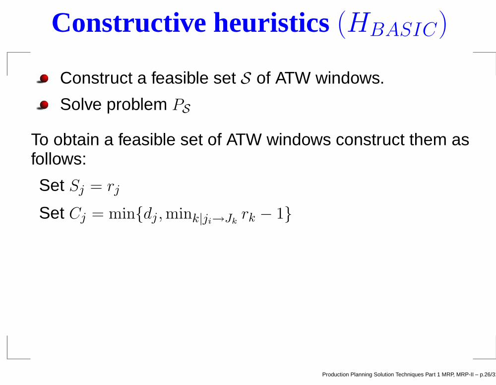
Constructive heuristics (HBASIC)
Construct a feasible set S of ATW windows.
Production Planning Solution Techniques Part 1 MRP, MRP-II – p.26/31
Constructive heuristics (HBASIC)
Construct a feasible set S of ATW windows.
Solve problem PS
Production Planning Solution Techniques Part 1 MRP, MRP-II – p.26/31
Constructive heuristics (HBASIC)
Construct a feasible set S of ATW windows.
Solve problem PS
To obtain a feasible set of ATW windows construct them asfollows:
Production Planning Solution Techniques Part 1 MRP, MRP-II – p.26/31
Constructive heuristics (HBASIC)
Construct a feasible set S of ATW windows.
Solve problem PS
To obtain a feasible set of ATW windows construct them asfollows:
Set Sj = rj
Production Planning Solution Techniques Part 1 MRP, MRP-II – p.26/31
Constructive heuristics (HBASIC)
Construct a feasible set S of ATW windows.
Solve problem PS
To obtain a feasible set of ATW windows construct them asfollows:
Set Sj = rj
Set Cj = min{dj ,mink|ji→Jkrk − 1}
Production Planning Solution Techniques Part 1 MRP, MRP-II – p.26/31

Constructive heuristics (HBASIC)
Construct a feasible set S of ATW windows.
Solve problem PS
To obtain a feasible set of ATW windows construct them asfollows:
Set Sj = rj
Set Cj = min{dj ,mink|ji→Jkrk − 1}
Have I forgotten an important assumption ?
Production Planning Solution Techniques Part 1 MRP, MRP-II – p.26/31
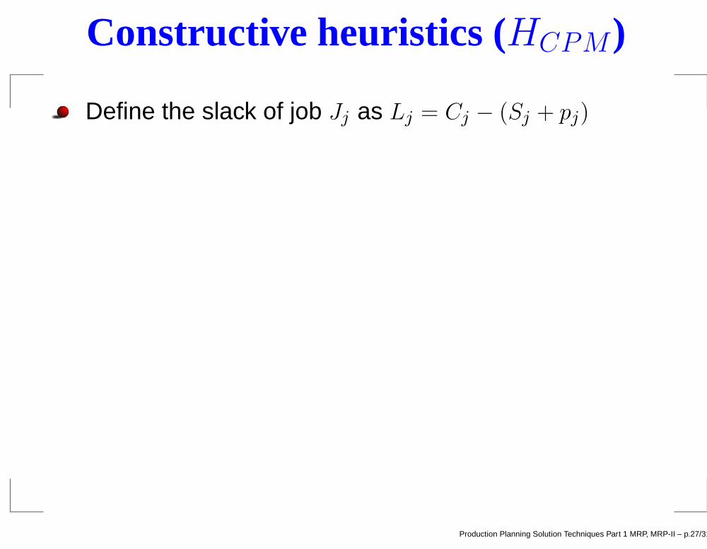
Constructive heuristics (HCPM)
Define the slack of job Jj as Lj = Cj − (Sj + pj)
Production Planning Solution Techniques Part 1 MRP, MRP-II – p.27/31

Constructive heuristics (HCPM)
Define the slack of job Jj as Lj = Cj − (Sj + pj)
{Ji1 , Ji2 , ·, Jik} is a ordered set if:
Production Planning Solution Techniques Part 1 MRP, MRP-II – p.27/31
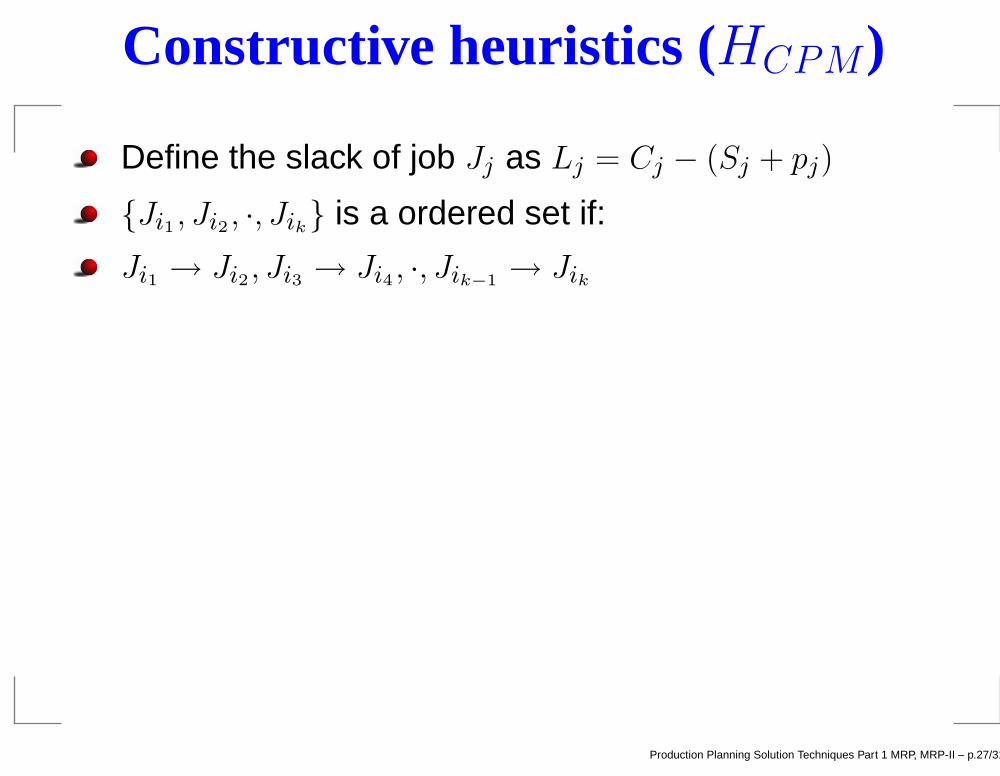
Constructive heuristics (HCPM)
Define the slack of job Jj as Lj = Cj − (Sj + pj)
{Ji1 , Ji2 , ·, Jik} is a ordered set if:
Ji1 → Ji2, Ji3 → Ji4 , ·, Jik−1→ Jik
Production Planning Solution Techniques Part 1 MRP, MRP-II – p.27/31
Constructive heuristics (HCPM)
Define the slack of job Jj as Lj = Cj − (Sj + pj)
{Ji1 , Ji2 , ·, Jik} is a ordered set if:
Ji1 → Ji2, Ji3 → Ji4 , ·, Jik−1→ Jik
A critical path is a path where:
Production Planning Solution Techniques Part 1 MRP, MRP-II – p.27/31

Constructive heuristics (HCPM)
Define the slack of job Jj as Lj = Cj − (Sj + pj)
{Ji1 , Ji2 , ·, Jik} is a ordered set if:
Ji1 → Ji2, Ji3 → Ji4 , ·, Jik−1→ Jik
A critical path is a path where:
Lj1 = Lj2 = · = min1≤n Lj
Production Planning Solution Techniques Part 1 MRP, MRP-II – p.27/31

Constructive heuristics (HCPM)
Define the slack of job Jj as Lj = Cj − (Sj + pj)
{Ji1 , Ji2 , ·, Jik} is a ordered set if:
Ji1 → Ji2, Ji3 → Ji4 , ·, Jik−1→ Jik
A critical path is a path where:
Lj1 = Lj2 = · = min1≤n Lj
Sji= Sji−1
+ pi−1 for2 ≤ i ≤ R
Production Planning Solution Techniques Part 1 MRP, MRP-II – p.27/31
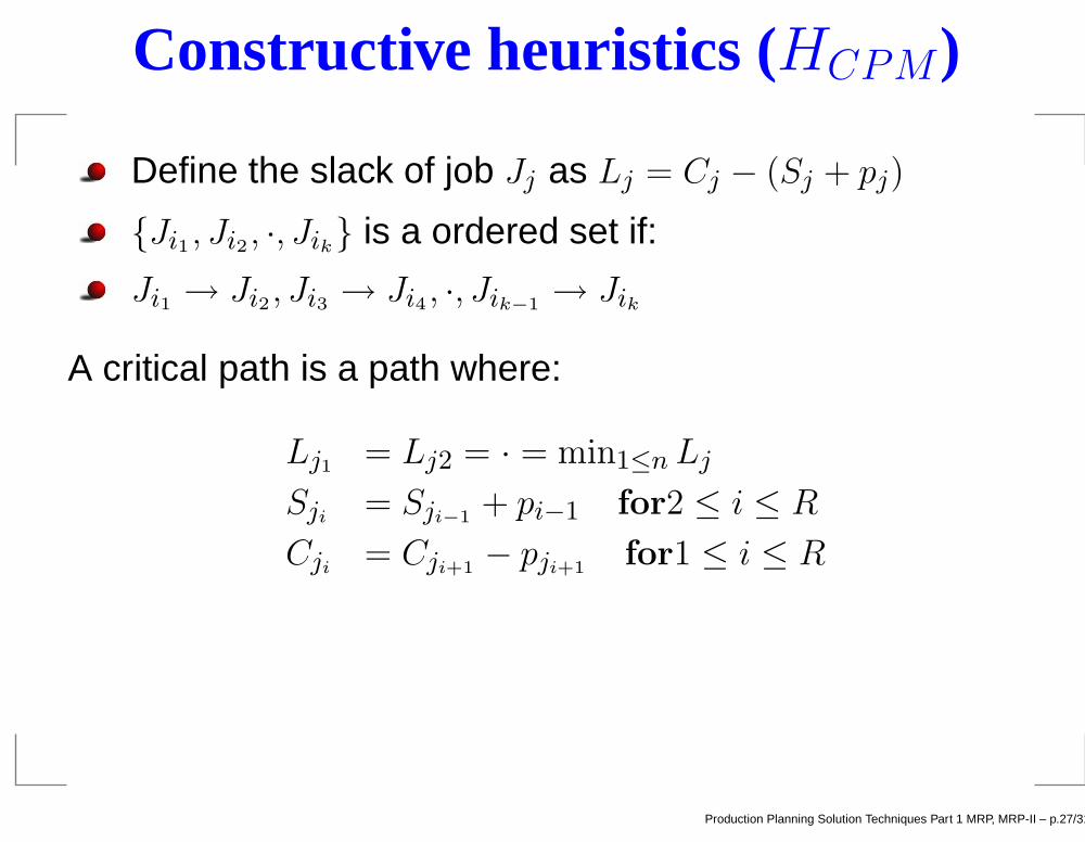
Constructive heuristics (HCPM)
Define the slack of job Jj as Lj = Cj − (Sj + pj)
{Ji1 , Ji2 , ·, Jik} is a ordered set if:
Ji1 → Ji2, Ji3 → Ji4 , ·, Jik−1→ Jik
A critical path is a path where:
Lj1 = Lj2 = · = min1≤n Lj
Sji= Sji−1
+ pi−1 for2 ≤ i ≤ R
Cji= Cji+1
− pji+1for1 ≤ i ≤ R
Production Planning Solution Techniques Part 1 MRP, MRP-II – p.27/31
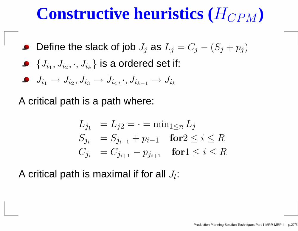
Constructive heuristics (HCPM)
Define the slack of job Jj as Lj = Cj − (Sj + pj)
{Ji1 , Ji2 , ·, Jik} is a ordered set if:
Ji1 → Ji2, Ji3 → Ji4 , ·, Jik−1→ Jik
A critical path is a path where:
Lj1 = Lj2 = · = min1≤n Lj
Sji= Sji−1
+ pi−1 for2 ≤ i ≤ R
Cji= Cji+1
− pji+1for1 ≤ i ≤ R
A critical path is maximal if for all Jl:
Production Planning Solution Techniques Part 1 MRP, MRP-II – p.27/31
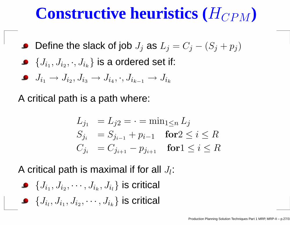
Constructive heuristics (HCPM)
Define the slack of job Jj as Lj = Cj − (Sj + pj)
{Ji1 , Ji2 , ·, Jik} is a ordered set if:
Ji1 → Ji2, Ji3 → Ji4 , ·, Jik−1→ Jik
A critical path is a path where:
Lj1 = Lj2 = · = min1≤n Lj
Sji= Sji−1
+ pi−1 for2 ≤ i ≤ R
Cji= Cji+1
− pji+1for1 ≤ i ≤ R
A critical path is maximal if for all Jl:
{Ji1 , Ji2 , · · · , Jik , Jil} is critical
{Jil, Ji1 , Ji2 , · · · , Jik} is critical
Production Planning Solution Techniques Part 1 MRP, MRP-II – p.27/31

(HCPM) continued
Initialize Sj = rj and Cj = dj for all Jj
Production Planning Solution Techniques Part 1 MRP, MRP-II – p.28/31
(HCPM) continued
Initialize Sj = rj and Cj = dj for all Jj
Compute the slack for all jobs
Production Planning Solution Techniques Part 1 MRP, MRP-II – p.28/31
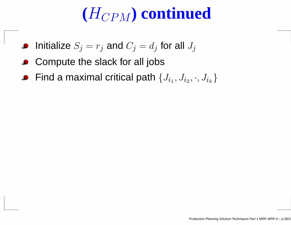
(HCPM) continued
Initialize Sj = rj and Cj = dj for all Jj
Compute the slack for all jobs
Find a maximal critical path {Ji1 , Ji2 , ·, Jik}
Production Planning Solution Techniques Part 1 MRP, MRP-II – p.28/31
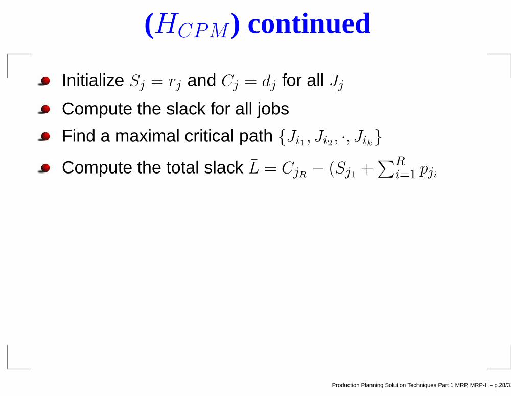
(HCPM) continued
Initialize Sj = rj and Cj = dj for all Jj
Compute the slack for all jobs
Find a maximal critical path {Ji1 , Ji2 , ·, Jik}
Compute the total slack L = CjR− (Sj1 +
∑Ri=1
pji
Production Planning Solution Techniques Part 1 MRP, MRP-II – p.28/31
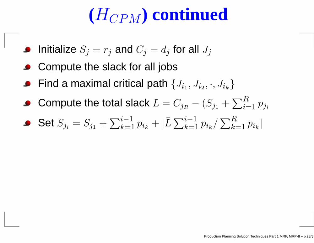
(HCPM) continued
Initialize Sj = rj and Cj = dj for all Jj
Compute the slack for all jobs
Find a maximal critical path {Ji1 , Ji2 , ·, Jik}
Compute the total slack L = CjR− (Sj1 +
∑Ri=1
pji
Set Sji= Sj1 +
∑i−1
k=1pik + |L
∑i−1
k=1pik/
∑Rk=1
pik |
Production Planning Solution Techniques Part 1 MRP, MRP-II – p.28/31
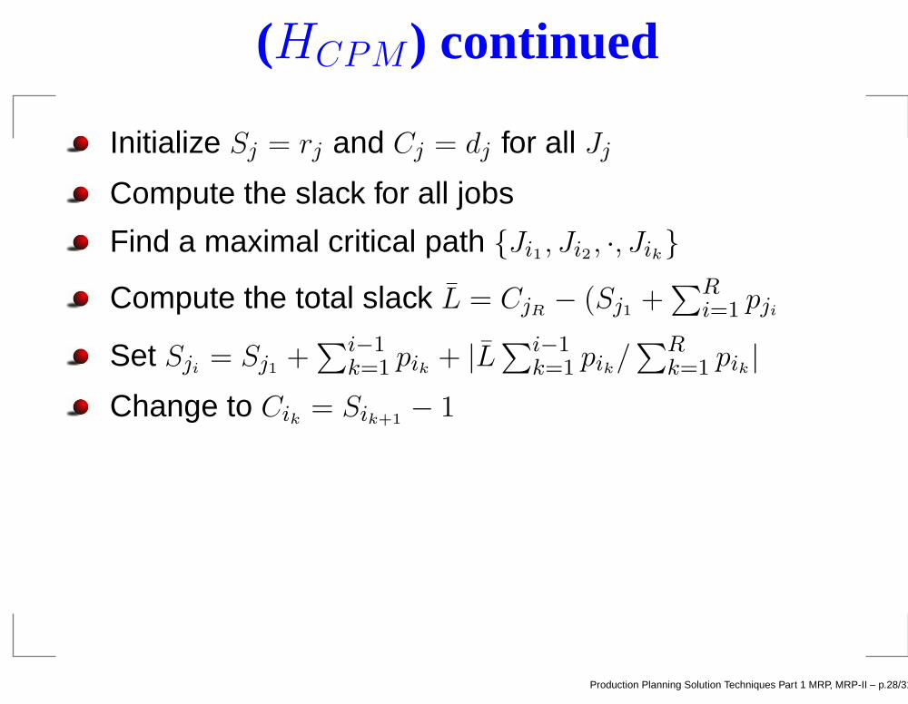
(HCPM) continued
Initialize Sj = rj and Cj = dj for all Jj
Compute the slack for all jobs
Find a maximal critical path {Ji1 , Ji2 , ·, Jik}
Compute the total slack L = CjR− (Sj1 +
∑Ri=1
pji
Set Sji= Sj1 +
∑i−1
k=1pik + |L
∑i−1
k=1pik/
∑Rk=1
pik |
Change to Cik = Sik+1− 1
Production Planning Solution Techniques Part 1 MRP, MRP-II – p.28/31
HCPM example
1 2 3 4S 0 5 15 20C 10 15 25 30p 5 5 10 5
Production Planning Solution Techniques Part 1 MRP, MRP-II – p.29/31

HCPM example
1 2 3 4S 0 5 15 20C 10 15 25 30p 5 5 10 5
L = C4 − (0 + 20) = 5
Production Planning Solution Techniques Part 1 MRP, MRP-II – p.29/31
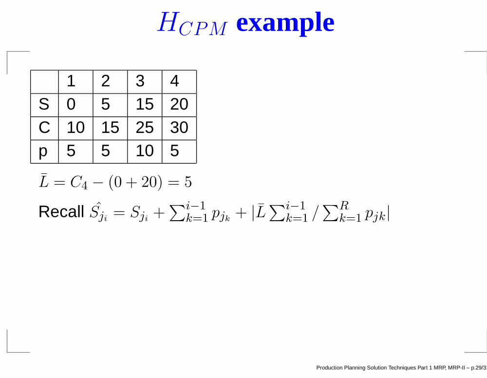
HCPM example
1 2 3 4S 0 5 15 20C 10 15 25 30p 5 5 10 5
L = C4 − (0 + 20) = 5
Recall Sji= Sji
+∑i−1
k=1pjk
+ |L∑i−1
k=1/∑R
k=1pjk|
Production Planning Solution Techniques Part 1 MRP, MRP-II – p.29/31
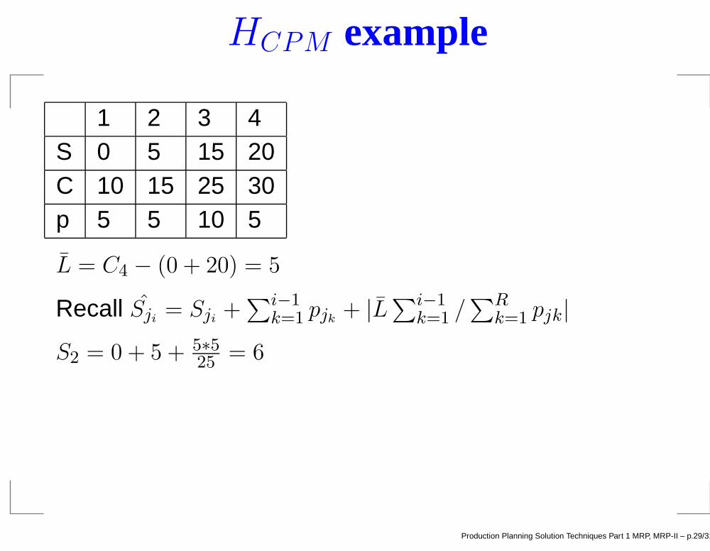
HCPM example
1 2 3 4S 0 5 15 20C 10 15 25 30p 5 5 10 5
L = C4 − (0 + 20) = 5
Recall Sji= Sji
+∑i−1
k=1pjk
+ |L∑i−1
k=1/∑R
k=1pjk|
S2 = 0 + 5 + 5∗525
= 6
Production Planning Solution Techniques Part 1 MRP, MRP-II – p.29/31
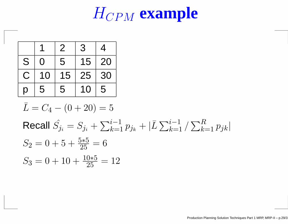
HCPM example
1 2 3 4S 0 5 15 20C 10 15 25 30p 5 5 10 5
L = C4 − (0 + 20) = 5
Recall Sji= Sji
+∑i−1
k=1pjk
+ |L∑i−1
k=1/∑R
k=1pjk|
S2 = 0 + 5 + 5∗525
= 6
S3 = 0 + 10 + 10∗525
= 12
Production Planning Solution Techniques Part 1 MRP, MRP-II – p.29/31
HCPM example
1 2 3 4S 0 5 15 20C 10 15 25 30p 5 5 10 5
L = C4 − (0 + 20) = 5
Recall Sji= Sji
+∑i−1
k=1pjk
+ |L∑i−1
k=1/∑R
k=1pjk|
S2 = 0 + 5 + 5∗525
= 6
S3 = 0 + 10 + 10∗525
= 12
S4 = 0 + 20 + 20∗525
= 24
Production Planning Solution Techniques Part 1 MRP, MRP-II – p.29/31

HCPM example
1 2 3 4S 0 5 15 20C 10 15 25 30p 5 5 10 5
L = C4 − (0 + 20) = 5
Recall Sji= Sji
+∑i−1
k=1pjk
+ |L∑i−1
k=1/∑R
k=1pjk|
S2 = 0 + 5 + 5∗525
= 6
S3 = 0 + 10 + 10∗525
= 12
S4 = 0 + 20 + 20∗525
= 24
C1 = S2 − 1 = 5, C2 = 11, C3 = 23
Production Planning Solution Techniques Part 1 MRP, MRP-II – p.29/31
Neighbourhoods
Production Planning Solution Techniques Part 1 MRP, MRP-II – p.30/31

Neighbourhoods
For job Jj increase Sj or decrease Cj
Production Planning Solution Techniques Part 1 MRP, MRP-II – p.30/31

Neighbourhoods
For job Jj increase Sj or decrease Cj
Decrease Sj implies Sj > rj, Ck = Sj − 1 for anypreceding job Jk and Ck − Sk ≥ pk
Production Planning Solution Techniques Part 1 MRP, MRP-II – p.30/31

Neighbourhoods
For job Jj increase Sj or decrease Cj
Decrease Sj implies Sj > rj, Ck = Sj − 1 for anypreceding job Jk and Ck − Sk ≥ pk
Neighbourhood can be ordered after the greedy choiceor the steepest edge rule.
Production Planning Solution Techniques Part 1 MRP, MRP-II – p.30/31

Exercises
Ex 1 Suggest some improvements for 2-3 of themodules in the MRP II model. You should describewhat additional data the system and need and whatvalue it would add for the users.
Production Planning Solution Techniques Part 1 MRP, MRP-II – p.31/31
Exercises
Ex 1 Suggest some improvements for 2-3 of themodules in the MRP II model. You should describewhat additional data the system and need and whatvalue it would add for the users.
Ex 2 For RCCP we have focused on the time drivencase in this exercise we consider the resource drivencase:
Ex 2.1 Give a mathematical model for the Resourcedriven RCCP without precedence constraints.
Production Planning Solution Techniques Part 1 MRP, MRP-II – p.31/31
Exercises
Ex 1 Suggest some improvements for 2-3 of themodules in the MRP II model. You should describewhat additional data the system and need and whatvalue it would add for the users.
Ex 2 For RCCP we have focused on the time drivencase in this exercise we consider the resource drivencase:
Ex 2.1 Give a mathematical model for the Resourcedriven RCCP without precedence constraints.Ex 2.2 If we use HBASIC to solve the resource drivenRCCP will it result in a feasible solution ? Justify youanswer
Production Planning Solution Techniques Part 1 MRP, MRP-II – p.31/31
Exercises
Ex 1 Suggest some improvements for 2-3 of themodules in the MRP II model. You should describewhat additional data the system and need and whatvalue it would add for the users.
Ex 2 For RCCP we have focused on the time drivencase in this exercise we consider the resource drivencase:
Ex 2.1 Give a mathematical model for the Resourcedriven RCCP without precedence constraints.Ex 2.2 If we use HBASIC to solve the resource drivenRCCP will it result in a feasible solution ? Justify youanswerEx 2.3 Describe a heuristic for the resource drivenRCCP. The heuristic should include a constructiveheuristic and a improvement heuristic.
Production Planning Solution Techniques Part 1 MRP, MRP-II – p.31/31


