ProE Mechanica 2001 Student Edition Tutor

SDC

Catalog

Pro/ENGINEER Tutorial & MultiMedia CD text by Roger Toogood / CD by Jack Zecher

The print version of the tutorial included with the Student Edition along with the MultiMedia CD.

For Release 2001.

Design Modeling with Pro/ENGINEER by James Bolluyt

The textbook style approach introduces users to the drawing capabilities of Pro/ENGINEER.

For Release 2001.

Pro/MECHANICA Structure Tutorial by Roger Toogood

This tutorial is written for first time FEA users (in general) and Pro/ MECHANICA users (in particular). Integrated Mode.

For Release 2001.

A Pro/MANUFACTURING Tutorial by Paul Funk & Loren Begley, Jr.

A tutorial for new users of Pro/MANUFACTURING, this book assumes a basic working knowledge of Pro/ENGINEER.

For Release 2001.

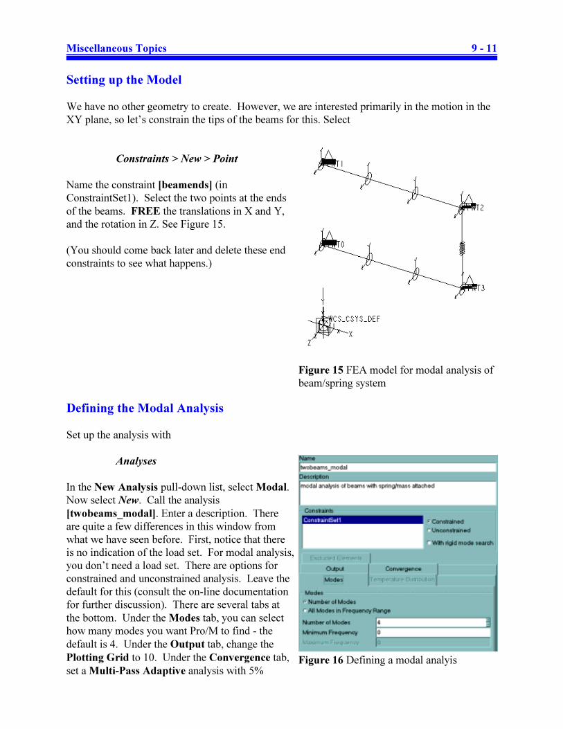
Parametric Modeling with Pro/ENGINEER by Randy Shih

The primary goal of this book is to introduce the aspects of Solid Modeling and Parametric Modeling.

For Release 2001.

Applications in Sheet Metal: Using Pro/SHEETMETAL and Pro/ENGINEER by David C. Planchard & Marie P. Planchard

A tutorial style introduction to Pro/SHEETMETAL. The textbook guides the user through seven sheetmetal projects.

For Release 2001.

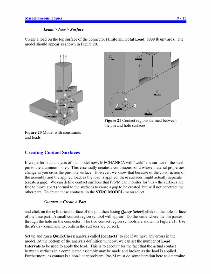
PUBLICATIONS

For more information, current catalog listings, or to order books,

please go online to:

www.JourneyEd.com

Mechanical Engineering Design with Pro/ENGINEER by Mark Archibald

This manual is written to teach students mechanical engineering design using Pro/ENGINEER software.

For Release 2001.

Pro/MECHANICA Structure

Release 2001 - Integrated Mode

Student Edition Tutorial

Roger Toogood, Ph.D., P. Eng.Mechanical EngineeringUniversity of Alberta

SDCSchroff Development Corporation

www.schroff.com

PUBLICATIONS

i

Pro/MECHANICA Structure Tutorial

Release 2001 - Integrated Mode

Preface

In his excellent text Finite Element Procedures, K.J. Bathe identifies two possible and different

objectives for studying Finite Element Analysis (FEA) and methods: to learn the proper use of

the method to solve complex problems (the practitioner’s goal), and to understand the methods

themselves in depth so as to pursue further development of the theory (the researcher’s goal).

This tutorial was created with the former objective in mind, recognizing that this is a formidable

task and not one that can be totally accomplished in a single, short volume. Thus, the primary

purpose of the tutorial is to introduce new users to Pro/MECHANICA® (Parametric Technology

Corporation, Waltham, MA) and see how it can be used to analyze a variety of problems.

The tutorial lessons cover most of the major concepts and frequently used commands required to

progress from a novice to an intermediate user level. The commands are presented in a click-by-

click manner using simple examples and exercises that illustrate a broad range of the most

common analysis types that can be performed. In addition to showing/illustrating the command

usage, the text will explain why certain commands are being used and, where appropriate, the

relation of commands to the overall FEA philosophy. Moreover, since error analysis is an

important skill, considerable time is spent exploring the created models (in fact, sometimes

intentionally inducing some errors), so that users will become comfortable with the "debugging"

phase of model creation.

In this 5th edition, the tutorial has been updated to Release 2001. The tutorial has been

extensively reorganized so that it deals exclusively with operation in integrated mode with

Pro/ENGINEER® 2001. A companion book from SDC deals with using Pro/M in independent

mode. Many problem types (in addition to solids) can be treated in integrated mode. These

include 2D models (plane stress/strain and axisymmetric solids and shells) created using the

Pro/E interface. Shell and beam idealizations are also possible. Other recent enhancements to the

program include cyclic constraints, changes in the interface and operation of the program such as

the inclusion of simulation features in the model tree. Most of these are covered in this tutorial.

The capability (introduced in Release 2000i) to handle large deformation problems, that is

problems involving geometric non-linearity, has not been covered due to space restraints. In any

case, this functionality is of a significantly more advanced level than what is required (perhaps)

in an introductory tutorial.

Students with a broad range of backgrounds should be able to use this book. The approach taken

in the manual is meant to allow accessability to persons of all levels. These lessons, therefore,

were written for new users with no previous experience with FEA, although some familiarity

with computers and elementary strength of materials is assumed. Because the book deals

exclusively with integrated mode, familiarity with Pro/ENGINEER is assumed. However,

because the emphasis is on Pro/MECHANICA, the Pro/E models are not too complex and should

be easily created by novice users of that program.

ii

This book is NOT a complete reference manual for Pro/MECHANICA. There are several

thousand pages of reference manuals available on-line with the Pro/MECHANICA installation,

with good search tools and cross-referencing to allow users to find relevant material quickly.

The tutorial treats solid models first, as these are the default model type created in Pro/E. This is

followed later by model idealizations: plane stress, plane strain, shells, beams, frames, and

axisymmetric shells and solids, springs, masses, and so on.

It continues to be a challenge to decide what to include and what to exclude in this introduction

in terms of the command set within Pro/MECHANICA. The author can only hope that the

presented material will be found useful, and in the right dose! It has also been interesting to

design suitable demonstration problems that are interesting, feasible with the state of learning of

the user, physically meaningful, and illustrate a broad set of Pro/MECHANICA functionality - all

within the space of 200 or so pages. It is hoped that at least some of these goals have been

satisfied.

Although every effort has been made in proofreading the text, it is inevitable that errors will

appear. The author takes full responsibility for these and hopes they will not impede your

progress through the tutorial. Any comments, criticisms, and/or suggestions will be gratefully

received and acknowledged. You can reach the author by email at the address

[email protected].

Enjoy the book!

Notes to Instructors:

The tutorials consist of the following:

2 lessons on general introductory material (reading only, but important!)

2 lessons introducing the basic operations in Pro/M using solid models

4 lessons on model idealizations (shells, beams and frames, plane stress, etc)

1 lesson on miscellaneous topics

Each of these tutorial chapters will take between 1-1/2 to 3 hours to complete depending on the

ability and background of the student. Moreover, additional time would be beneficial for

experimentation and additional exploration of the program. Most of the material can be done by

the student on their own, however there are a few "tricky" bits in some of the lessons. Therefore,

it is important to have experienced and knowledgeable teaching assistants available (preferably

right in the computer lab) who can answer special questions and especially bail out students who

get into trouble. Most common causes of confusion are due to not completing the lessons or

digesting the material. This is not surprising given the volume of new information or the lack of

time in students’ schedules. However, I have found that most student questions are answered

within the lessons.

In addition to the tutorials, it is presumed that some class time over the duration of a course will

be used for discussion of some of the broader issues of FEA, such as the treatment of constraints.

iii

It is vitally important for students to compare their FEA results with other possible solutions.

This can be accomplished using simple problems for which either analytical solutions or

experimental data exist. An extended discussion and exploration of modeling of boundary

conditions would be very beneficial. It takes a while for students to realize that just creating the

model and producing pretty pictures is not sufficient for design work, and the notions of accuracy

and convergence need careful treatment and discussion.

It should be expected that most students, after having gone through a lesson only once, will not

have absorbed very much. My experience is that many students execute the commands without

reading or studying the accompanying text explaining why. The second pass through the lesson

usually results in considerably more retention and understanding. Each lesson concludes with a

number of review questions and simple exercises that can be completed using new commands

taught in that lesson. Where possible, students should be given additional problems that can be

verified independently by experiment or analytical methods. Students really don't feel

comfortable or confident until they can make models from scratch on their own.

That having been said, I am continually amazed at how quickly many students can get up the

learning curve on both Pro/ENGINEER and Pro/MECHANICA. Any instructor introducing this

software to a class of capable students should be prepared to move very quickly to stay ahead of

the class!

iv

Acknowledgments

Some of the models used in these tutorials are based on the treatment in The Finite Element

Method in Mechanical Design (PWS-Kent, 1993) by Charles E. Knight. This is a clearly

written and informative book, although emphasis is on the h-code analysis with only tangential

mention of the p-code method used in Pro/MECHANICA.

Thanks are due to Stephen Schroff and Mary Schmidt at Schroff Development Corporation and

Janet Drumm at JourneyEd for their efforts in taking this work to a wider audience and for their

tolerance of the delays in its arrival!

Finally, once again I must express special thanks due to my wife, Elaine, for her unflagging

support and tolerance of my many late nights, evenings, and weekends spent on this project, and

to our daughters Jenny and Kate for their patience when Daddy was preoccupied with this work.

And, as always, thanks are due to our good friends, Jayne and Rowan.

To users of this material, I hope you enjoy the lessons. I apologize beforehand for any omissions

and errors that may have appeared and I would appreciate any comments, criticisms, and

suggestions for the improvement of this manual.

RWT

Edmonton, Alberta

11 July 2001

DISCLAIMER

The discussion, examples, and exercises in this tutorial are meant only to demonstrate the

functionality of the program and are not to be construed as fully engineered design solutions for

any particular problem. Use of the methods and procedures described herein are for instructional

purposes only and are not warranted or guaranteed to provide satisfactory solutions in any

specific application. The author and publisher assume no responsibility or liability for any errors

or inaccuracies contained in the tutorial, or for any results or solutions obtained using the

methods and procedures described herein.

Pro/MECHANICA Structure Tutorial (Release 2001)

©2001 by ProCAD Engineering Ltd., Edmonton, Alberta. All rights reserved. This document

may not be copied, photocopied, reproduced, transmitted, or translated in any form or for any

purpose without the express written consent of the publisher Schroff Development Corporation.

Pro/ENGINEER and Pro/MECHANICA are registered trademarks, and all product names in the

PTC family are trademarks of Parametric Technology Corporation, Waltham, MA, U.S.A.

v

Organization and Synopsis of the Tutorials

A brief synopsis of the nine chapters in this book is given below. Each chapter should take at

least 1.5 to 3 hours to complete - if you go through the lessons too quickly or thoughtlessly, you

may not understand or remember the material. For best results, it is suggested that you

scan/browse through the lesson completely before going through it in detail. You will then have

a sense of where the lesson is going, and not be tempted to just follow the commands blindly.

You need to have a sense of the forest when examining each individual tree!

Chapter 1 - Introduction to MECHANICA

An introduction to finite element analysis, with some cautions about

its use and misuse; examples of problems solved with

MECHANICA; organization of the tutorials; tips and tricks for

using MECHANICA

Chapter 2 - Finite Element Modeling with MECHANICA

Background information on FEA. The concept of modeling. Particular

attention is directed at concerns of accuracy and convergence of

solutions, and the differences between h-code and p-code FEA.

Overview of MECHANICA operations and nomenclature

Chapter 3 - Solid Models (Part 1 - Static Analysis)

A simple model is created using Pro/ENGINEER and analyzed in

Pro/MECHANICA. The complete sequence of steps required for a

static analysis will be outlined, and basic result display options

presented. Automatic mesh generation.

Chapter 4 - Solid Models (Part 2 - Sensitivity Studies and Optimization)

Design parameters are designated for sensitivity studies and

optimization. Special concerns for applying loads and constraints

on solid models are explored. Superposition and multiple load sets

are introduced.

vi

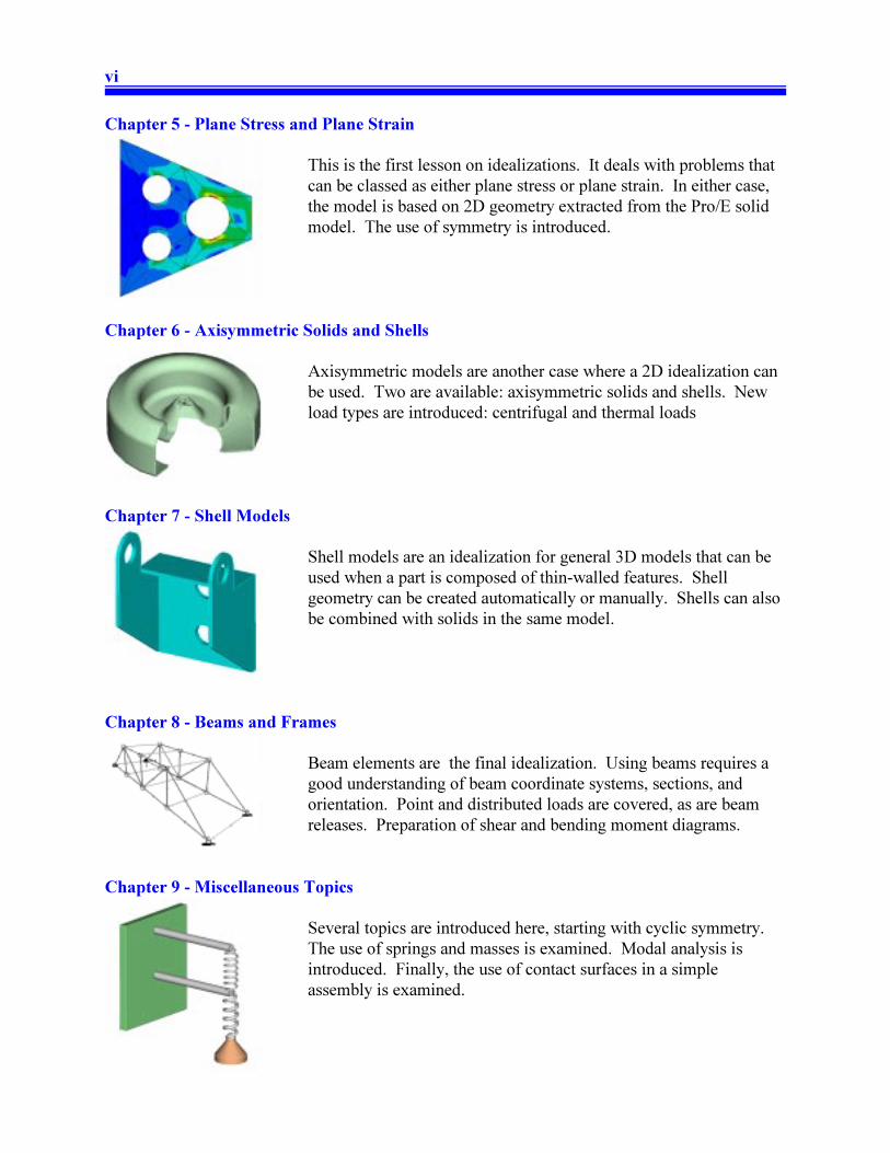
Chapter 5 - Plane Stress and Plane Strain

This is the first lesson on idealizations. It deals with problems that

can be classed as either plane stress or plane strain. In either case,

the model is based on 2D geometry extracted from the Pro/E solid

model. The use of symmetry is introduced.

Chapter 6 - Axisymmetric Solids and Shells

Axisymmetric models are another case where a 2D idealization can

be used. Two are available: axisymmetric solids and shells. New

load types are introduced: centrifugal and thermal loads

Chapter 7 - Shell Models

Shell models are an idealization for general 3D models that can be

used when a part is composed of thin-walled features. Shell

geometry can be created automatically or manually. Shells can also

be combined with solids in the same model.

Chapter 8 - Beams and Frames

Beam elements are the final idealization. Using beams requires a

good understanding of beam coordinate systems, sections, and

orientation. Point and distributed loads are covered, as are beam

releases. Preparation of shear and bending moment diagrams.

Chapter 9 - Miscellaneous Topics

Several topics are introduced here, starting with cyclic symmetry.

The use of springs and masses is examined. Modal analysis is

introduced. Finally, the use of contact surfaces in a simple

assembly is examined.

vii

TABLE OF CONTENTS

Preface i

Note to Instructors ii

Acknowledgments iv

Organization and Synopsis of Tutorials v

Table of Contents vii

Chapter 1 - Introduction to the Tutorials

Synopsis . . . . . . . . . . . . . . . . . . . . . . . . . . . . . . . . . . . . . . . . . . . . . . . . . . . . . . . . . . . . . . . . . . 1 - 1

Overview of this Lesson . . . . . . . . . . . . . . . . . . . . . . . . . . . . . . . . . . . . . . . . . . . . . . . . . . . . . 1 - 1

Finite Element Analysis . . . . . . . . . . . . . . . . . . . . . . . . . . . . . . . . . . . . . . . . . . . . . . . . . . . . . . 1 - 1

Examples of Problems Solved using MECHANICA . . . . . . . . . . . . . . . . . . . . . . . . . . . . . . . 1 - 2

Example #1 : Analysis . . . . . . . . . . . . . . . . . . . . . . . . . . . . . . . . . . . . . . . . . . . . . . . . . . 1 - 3

Example #2 : Sensitivity Study . . . . . . . . . . . . . . . . . . . . . . . . . . . . . . . . . . . . . . . . . . . . 1 - 4

Example #3 : Design Optimization . . . . . . . . . . . . . . . . . . . . . . . . . . . . . . . . . . . . . . . . . 1 - 5

FEA User Beware! . . . . . . . . . . . . . . . . . . . . . . . . . . . . . . . . . . . . . . . . . . . . . . . . . . . . . . . . . . 1 - 7

Layout of this Manual . . . . . . . . . . . . . . . . . . . . . . . . . . . . . . . . . . . . . . . . . . . . . . . . . . . . . . . 1 - 9

Tips for using MECHANICA . . . . . . . . . . . . . . . . . . . . . . . . . . . . . . . . . . . . . . . . . . . . . . . . 1 - 10

Chapter 2 - Finite Element Modeling with MECHANICA

Synopsis . . . . . . . . . . . . . . . . . . . . . . . . . . . . . . . . . . . . . . . . . . . . . . . . . . . . . . . . . . . . . . . . . . 2 - 1


Finite Element Analysis : An Introduction . . . . . . . . . . . . . . . . . . . . . . . . . . . . . . . . . . . . . . . 2 - 1

The FEA Model and General Processing Steps . . . . . . . . . . . . . . . . . . . . . . . . . . . . . . . 2 - 4

Steps in Preparing an FEA Model for Solution . . . . . . . . . . . . . . . . . . . . . . . . . . . . . . . 2 - 6

P-Elements versus H-Elements . . . . . . . . . . . . . . . . . . . . . . . . . . . . . . . . . . . . . . . . . . . . . . . . 2 - 7

Convergence of H-elements (the “classic” approach) . . . . . . . . . . . . . . . . . . . . . . . . . . . 2 - 7

Convergence of P-elements (the Pro/MECHANICA approach) . . . . . . . . . . . . . . . . . . . 2 - 9

Convergence and Accuracy in the Solution . . . . . . . . . . . . . . . . . . . . . . . . . . . . . . . . . . . . . . 2 - 10

Sources of Error . . . . . . . . . . . . . . . . . . . . . . . . . . . . . . . . . . . . . . . . . . . . . . . . . . . . . . 2 - 11

A CAD Model is NOT an FEA Model! . . . . . . . . . . . . . . . . . . . . . . . . . . . . . . . . . . . . . . . . . 2 - 12

Overview of Pro/MECHANICA Structure . . . . . . . . . . . . . . . . . . . . . . . . . . . . . . . . . . . . . . 2 - 14

Basic Operation . . . . . . . . . . . . . . . . . . . . . . . . . . . . . . . . . . . . . . . . . . . . . . . . . . . . . . . 2 - 14

TABLE I - An Overall View of Pro/M Capability and Function . . . . . . . . . . . . . 2 - 14

Modes of Operation . . . . . . . . . . . . . . . . . . . . . . . . . . . . . . . . . . . . . . . . . . . . . . . 2 - 15

TABLE II - Pro/MECHANICA Modes of Operation . . . . . . . . . . . . . . . . . . . . . 2 - 16

Types of Models . . . . . . . . . . . . . . . . . . . . . . . . . . . . . . . . . . . . . . . . . . . . . . . . . . 2 - 16

Types of Elements . . . . . . . . . . . . . . . . . . . . . . . . . . . . . . . . . . . . . . . . . . . . . . . . 2 - 16

Analysis Methods . . . . . . . . . . . . . . . . . . . . . . . . . . . . . . . . . . . . . . . . . . . . . . . . . 2 - 17

Convergence Methods . . . . . . . . . . . . . . . . . . . . . . . . . . . . . . . . . . . . . . . . . . . . . 2 - 17

Design Studies . . . . . . . . . . . . . . . . . . . . . . . . . . . . . . . . . . . . . . . . . . . . . . . . . . . 2 - 17

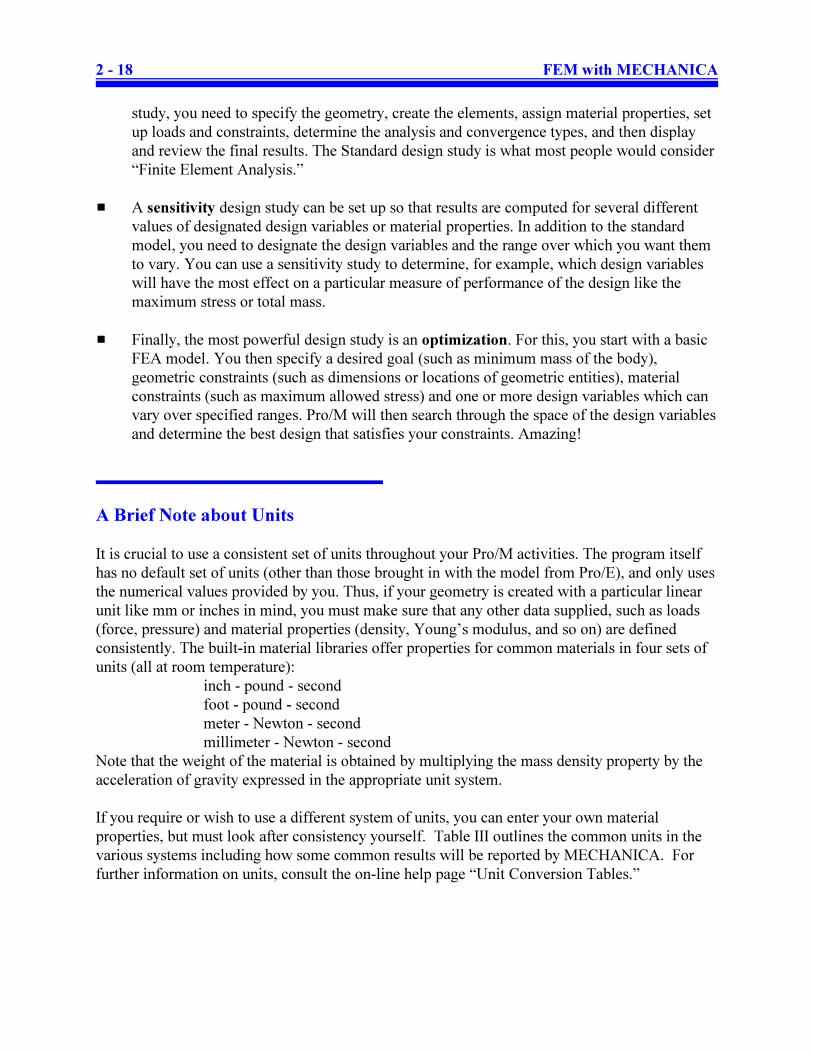
A Brief Note about Units . . . . . . . . . . . . . . . . . . . . . . . . . . . . . . . . . . . . . . . . . . . . . . . 2 - 18

viii

TABLE III - Common unit systems in Pro/MECHANICA . . . . . . . . . . . . . . . . . 2 - 19

Files and Directories Produced by Pro/MECHANICA . . . . . . . . . . . . . . . . . . . . . . . . . 2 - 19

Table IV - Some Files Produced by Pro/MECHANICA . . . . . . . . . . . . . . . . . . . 2 - 20

On-line Documentation . . . . . . . . . . . . . . . . . . . . . . . . . . . . . . . . . . . . . . . . . . . . . . . . . 2 - 20

Summary . . . . . . . . . . . . . . . . . . . . . . . . . . . . . . . . . . . . . . . . . . . . . . . . . . . . . . . . . . . . . . . . 2 - 21

References . . . . . . . . . . . . . . . . . . . . . . . . . . . . . . . . . . . . . . . . . . . . . . . . . . . . . . . . . . . . . . . 2 - 21

Chapter 3 - Solid Models (Part 1)

Synopsis . . . . . . . . . . . . . . . . . . . . . . . . . . . . . . . . . . . . . . . . . . . . . . . . . . . . . . . . . . . . . . . . . . 3 - 1


Simple Static Analysis of a Solid Part . . . . . . . . . . . . . . . . . . . . . . . . . . . . . . . . . . . . . . . . . . . 3 - 2

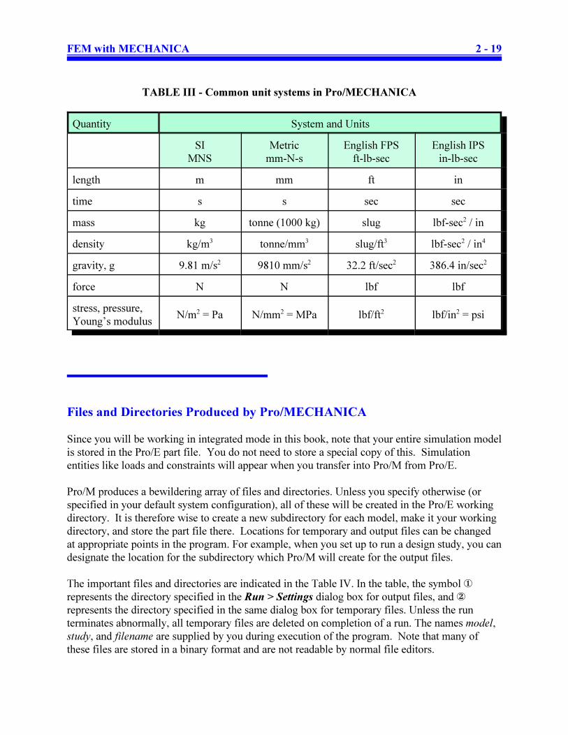
Creating the Geometry of the Model . . . . . . . . . . . . . . . . . . . . . . . . . . . . . . . . . . . . . . . 3 - 2

Setting up the FEA Model . . . . . . . . . . . . . . . . . . . . . . . . . . . . . . . . . . . . . . . . . . . . . . . 3 - 3

Launching Pro/Mechanica . . . . . . . . . . . . . . . . . . . . . . . . . . . . . . . . . . . . . . . . . . . 3 - 3

Applying the Constraints . . . . . . . . . . . . . . . . . . . . . . . . . . . . . . . . . . . . . . . . . . . . 3 - 4

Applying the Loads . . . . . . . . . . . . . . . . . . . . . . . . . . . . . . . . . . . . . . . . . . . . . . . . 3 - 6

Specifying the Material . . . . . . . . . . . . . . . . . . . . . . . . . . . . . . . . . . . . . . . . . . . . . 3 - 7

Setting up the Analysis . . . . . . . . . . . . . . . . . . . . . . . . . . . . . . . . . . . . . . . . . . . . . 3 - 8

Running the Analysis . . . . . . . . . . . . . . . . . . . . . . . . . . . . . . . . . . . . . . . . . . . . . . . . . . . 3 - 9

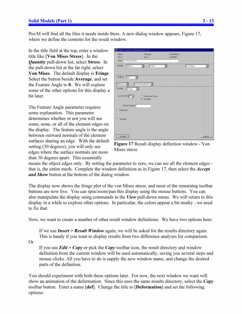
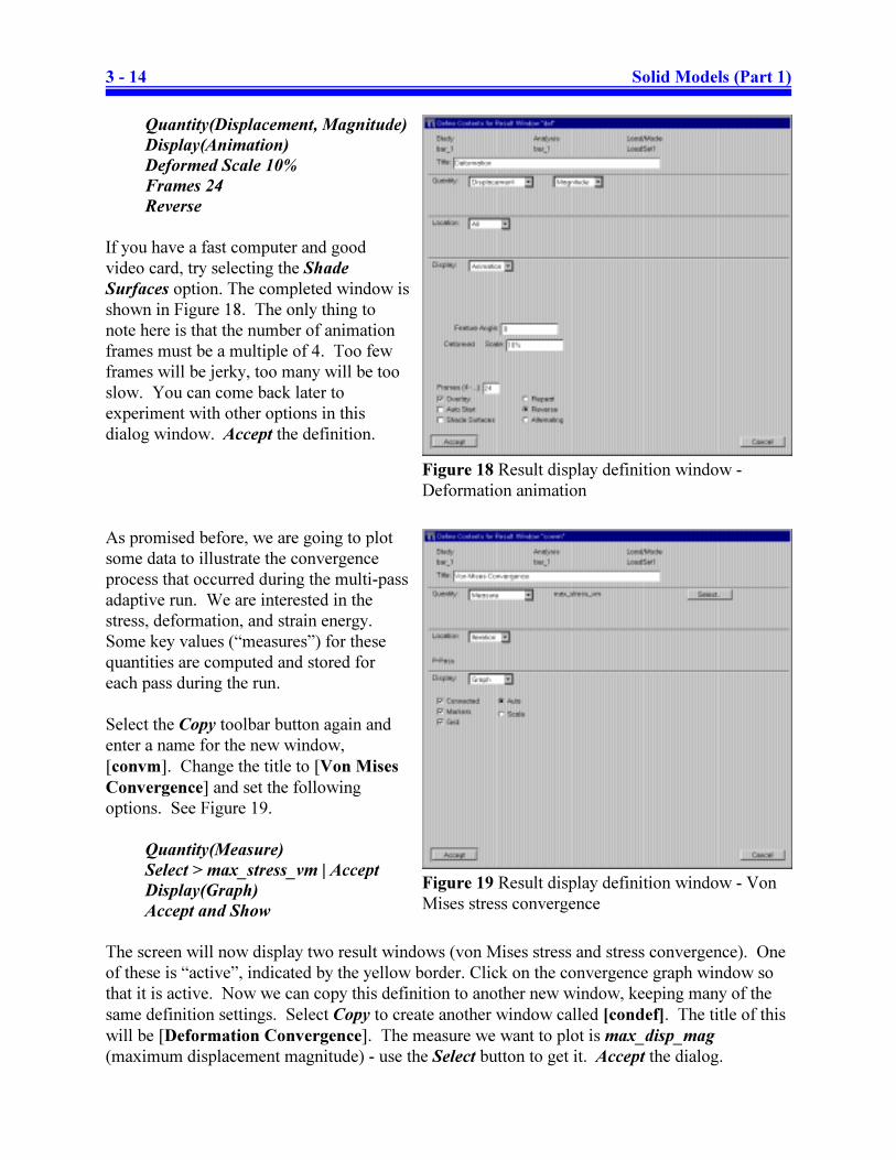
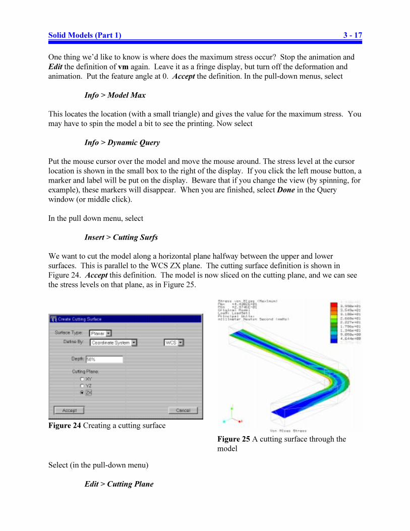
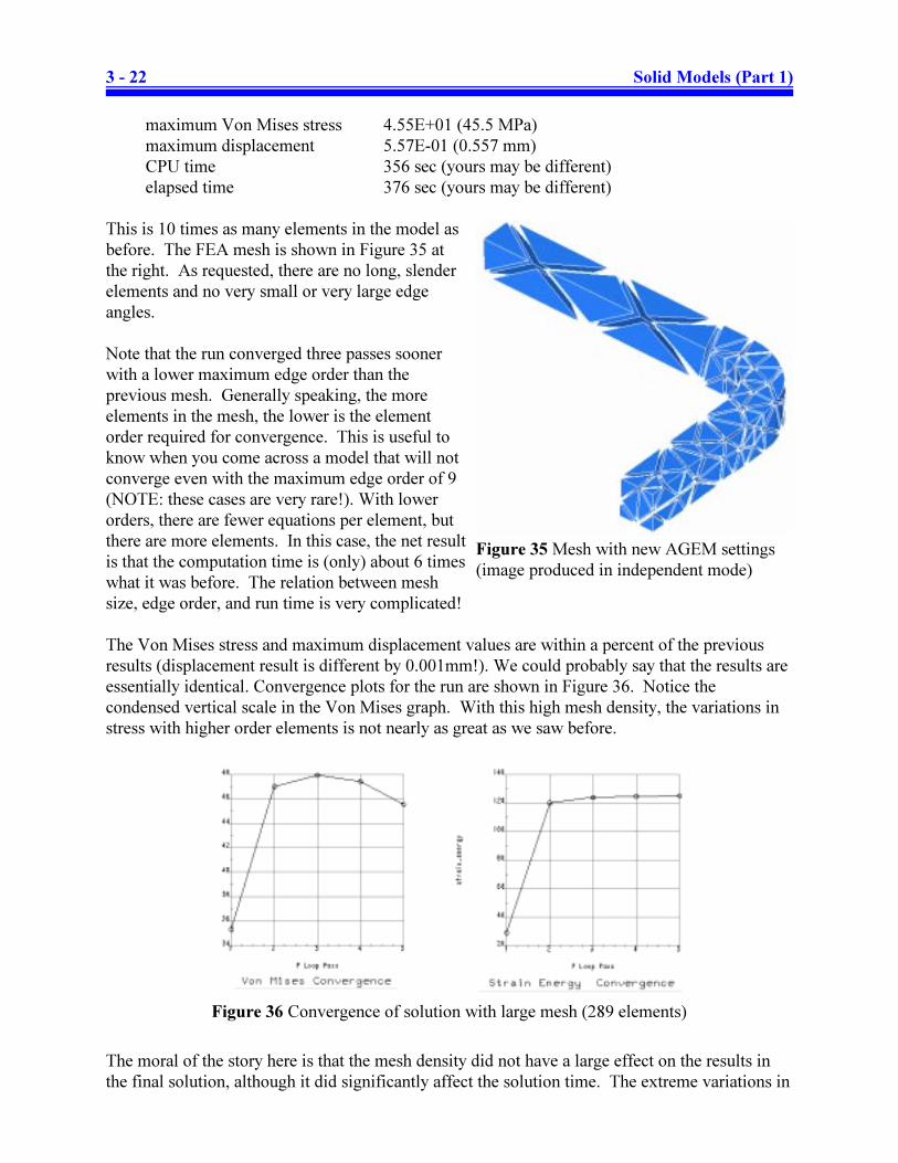
Displaying the Results . . . . . . . . . . . . . . . . . . . . . . . . . . . . . . . . . . . . . . . . . . . . . . . . . 3 - 11

Creating Result Window Definitions . . . . . . . . . . . . . . . . . . . . . . . . . . . . . . . . . . 3 - 11

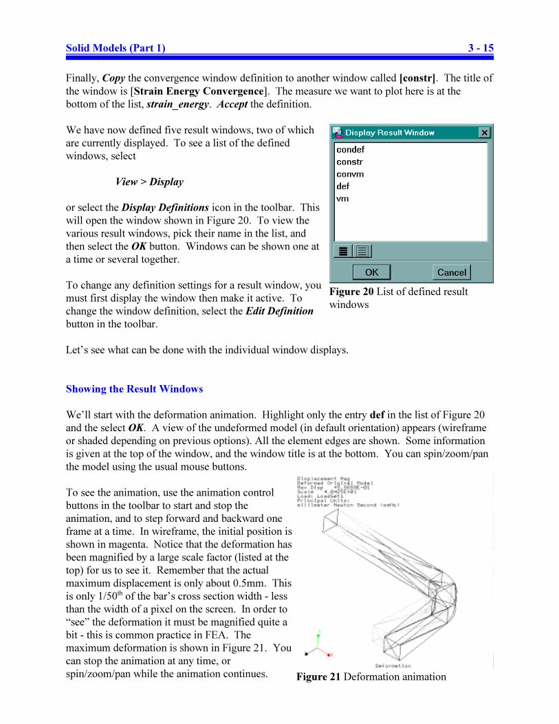
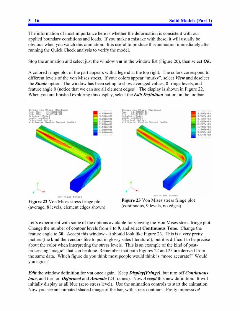
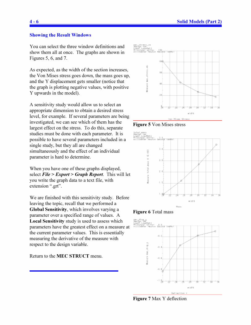
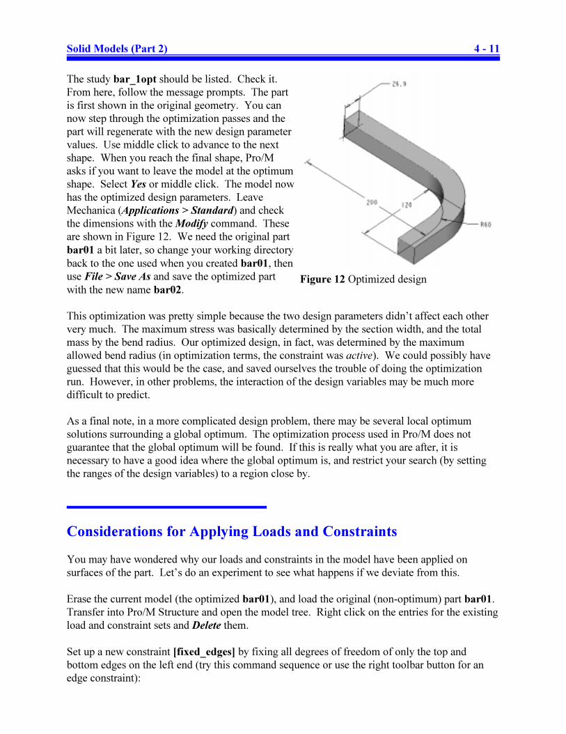
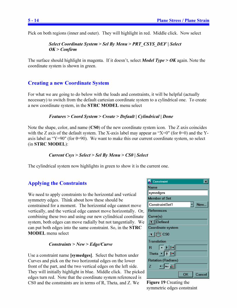
Showing the Result Windows . . . . . . . . . . . . . . . . . . . . . . . . . . . . . . . . . . . . . . . 3 - 15

Simulation Features in the Model Tree . . . . . . . . . . . . . . . . . . . . . . . . . . . . . . . . . . . . . . . . . 3 - 19

Exploring the FEA Mesh and AutoGEM . . . . . . . . . . . . . . . . . . . . . . . . . . . . . . . . . . . . . . . . 3 - 19

Running the Model in Pro/M Independent Mode . . . . . . . . . . . . . . . . . . . . . . . . . . . . . 3 - 23

Summary . . . . . . . . . . . . . . . . . . . . . . . . . . . . . . . . . . . . . . . . . . . . . . . . . . . . . . . . . . . . . . . . 3 - 24

Chapter 4 - Solid Models (Part 2)

Synopsis . . . . . . . . . . . . . . . . . . . . . . . . . . . . . . . . . . . . . . . . . . . . . . . . . . . . . . . . . . . . . . . . . . 4 - 1


Sensitivity Studies . . . . . . . . . . . . . . . . . . . . . . . . . . . . . . . . . . . . . . . . . . . . . . . . . . . . . . . . . . 4 - 2

Creating a Design Variable . . . . . . . . . . . . . . . . . . . . . . . . . . . . . . . . . . . . . . . . . . . . . . . 4 - 2

Setting up the Design Study . . . . . . . . . . . . . . . . . . . . . . . . . . . . . . . . . . . . . . . . . . . . . . 4 - 4

Running the Design Study . . . . . . . . . . . . . . . . . . . . . . . . . . . . . . . . . . . . . . . . . . . . . . . 4 - 5

Displaying the Results . . . . . . . . . . . . . . . . . . . . . . . . . . . . . . . . . . . . . . . . . . . . . . . . . . 4 - 5

Creating Result Window Definitions . . . . . . . . . . . . . . . . . . . . . . . . . . . . . . . . . . . 4 - 5

Showing the Result Windows . . . . . . . . . . . . . . . . . . . . . . . . . . . . . . . . . . . . . . . . 4 - 6

Optimization . . . . . . . . . . . . . . . . . . . . . . . . . . . . . . . . . . . . . . . . . . . . . . . . . . . . . . . . . . . . . . 4 - 7

Creating Design Parameters . . . . . . . . . . . . . . . . . . . . . . . . . . . . . . . . . . . . . . . . . . . . . . 4 - 7

Examining the Search Space . . . . . . . . . . . . . . . . . . . . . . . . . . . . . . . . . . . . . . . . . . . . . . 4 - 7

Creating the Optimization Design Study . . . . . . . . . . . . . . . . . . . . . . . . . . . . . . . . . . . . 4 - 8

Optimization Results . . . . . . . . . . . . . . . . . . . . . . . . . . . . . . . . . . . . . . . . . . . . . . . . . . . . 4 - 9

Considerations for Applying Loads and Constraints . . . . . . . . . . . . . . . . . . . . . . . . . . . . . . . 4 - 11

ix

Superposition and Multiple Load Sets . . . . . . . . . . . . . . . . . . . . . . . . . . . . . . . . . . . . . . . . . . 4 - 15

Creating Multiple Load Sets . . . . . . . . . . . . . . . . . . . . . . . . . . . . . . . . . . . . . . . . . . . . . 4 - 16

Setting the Analysis for Multiple Load Sets . . . . . . . . . . . . . . . . . . . . . . . . . . . . . . . . . 4 - 16

Combining Results for Multiple Load Sets . . . . . . . . . . . . . . . . . . . . . . . . . . . . . . . . . 4 - 17

Summary . . . . . . . . . . . . . . . . . . . . . . . . . . . . . . . . . . . . . . . . . . . . . . . . . . . . . . . . . . . . . . . . 4 - 20

Chapter 5 - Plane Stress and Plane Strain Models

Synopsis . . . . . . . . . . . . . . . . . . . . . . . . . . . . . . . . . . . . . . . . . . . . . . . . . . . . . . . . . . . . . . . . . . 5 - 1


Plane Stress Models . . . . . . . . . . . . . . . . . . . . . . . . . . . . . . . . . . . . . . . . . . . . . . . . . . . . . . . . . 5 - 2

Creating a Coordinate System . . . . . . . . . . . . . . . . . . . . . . . . . . . . . . . . . . . . . . . . . . . . . 5 - 3

Setting the Model Type . . . . . . . . . . . . . . . . . . . . . . . . . . . . . . . . . . . . . . . . . . . . . . . . . . 5 - 4

Applying Loads and Constraints . . . . . . . . . . . . . . . . . . . . . . . . . . . . . . . . . . . . . . . . . . . 5 - 4

Defining Model Properties . . . . . . . . . . . . . . . . . . . . . . . . . . . . . . . . . . . . . . . . . . . . . . . 5 - 5

Setting up and Running the Analysis . . . . . . . . . . . . . . . . . . . . . . . . . . . . . . . . . . . . . . . 5 - 6

Viewing the Results . . . . . . . . . . . . . . . . . . . . . . . . . . . . . . . . . . . . . . . . . . . . . . . . . . . . 5 - 6

Exploring Symmetry . . . . . . . . . . . . . . . . . . . . . . . . . . . . . . . . . . . . . . . . . . . . . . . . . . . . . . . . 5 - 8

Setting Constraints and Loads . . . . . . . . . . . . . . . . . . . . . . . . . . . . . . . . . . . . . . . . . . . . . 5 - 8

Running the Symmetric Half-Model . . . . . . . . . . . . . . . . . . . . . . . . . . . . . . . . . . . . . . . . 5 - 9

Plane Strain Models . . . . . . . . . . . . . . . . . . . . . . . . . . . . . . . . . . . . . . . . . . . . . . . . . . . . . . . . 5 - 11

The Model . . . . . . . . . . . . . . . . . . . . . . . . . . . . . . . . . . . . . . . . . . . . . . . . . . . . . . . . . . . 5 - 11

Creating the Pro/E Part . . . . . . . . . . . . . . . . . . . . . . . . . . . . . . . . . . . . . . . . . . . . . . . . . 5 - 12

Creating Surface Regions . . . . . . . . . . . . . . . . . . . . . . . . . . . . . . . . . . . . . . . . . . . . . . . 5 - 13

Setting the Model Type . . . . . . . . . . . . . . . . . . . . . . . . . . . . . . . . . . . . . . . . . . . . . . . . . 5 - 13

Creating a new Coordinate System . . . . . . . . . . . . . . . . . . . . . . . . . . . . . . . . . . . . . . . . 5 - 14

Applying the Constraints . . . . . . . . . . . . . . . . . . . . . . . . . . . . . . . . . . . . . . . . . . . . . . . 5 - 14

Applying a Pressure Load . . . . . . . . . . . . . . . . . . . . . . . . . . . . . . . . . . . . . . . . . . . . . . . 5 - 15

Applying a Temperature Load . . . . . . . . . . . . . . . . . . . . . . . . . . . . . . . . . . . . . . . . . . . 5 - 15

Specifying Materials . . . . . . . . . . . . . . . . . . . . . . . . . . . . . . . . . . . . . . . . . . . . . . . . . . . 5 - 16

Running the Model . . . . . . . . . . . . . . . . . . . . . . . . . . . . . . . . . . . . . . . . . . . . . . . . . . . . 5 - 17

Quick Check . . . . . . . . . . . . . . . . . . . . . . . . . . . . . . . . . . . . . . . . . . . . . . . . . . . . . 5 - 17

Multi-Pass Adaptive . . . . . . . . . . . . . . . . . . . . . . . . . . . . . . . . . . . . . . . . . . . . . . . 5 - 18

Viewing the Results . . . . . . . . . . . . . . . . . . . . . . . . . . . . . . . . . . . . . . . . . . . . . . . . . . . 5 - 18

Summary . . . . . . . . . . . . . . . . . . . . . . . . . . . . . . . . . . . . . . . . . . . . . . . . . . . . . . . . . . . . . . . . 5 - 20

Chapter 6 - Axisymmetric Solids and Shells

Synopsis . . . . . . . . . . . . . . . . . . . . . . . . . . . . . . . . . . . . . . . . . . . . . . . . . . . . . . . . . . . . . . . . . . 6 - 1


Axisymmetric Models . . . . . . . . . . . . . . . . . . . . . . . . . . . . . . . . . . . . . . . . . . . . . . . . . . . . . . . 6 - 1

Elements . . . . . . . . . . . . . . . . . . . . . . . . . . . . . . . . . . . . . . . . . . . . . . . . . . . . . . . . . . . . . 6 - 2

Loads . . . . . . . . . . . . . . . . . . . . . . . . . . . . . . . . . . . . . . . . . . . . . . . . . . . . . . . . . . . . . . . . 6 - 2

Constraints . . . . . . . . . . . . . . . . . . . . . . . . . . . . . . . . . . . . . . . . . . . . . . . . . . . . . . . . . . . 6 - 3

Restrictions . . . . . . . . . . . . . . . . . . . . . . . . . . . . . . . . . . . . . . . . . . . . . . . . . . . . . . . . . . . 6 - 3

x

Axisymmetric Solids . . . . . . . . . . . . . . . . . . . . . . . . . . . . . . . . . . . . . . . . . . . . . . . . . . . . . . . . 6 - 3

Creating the Model . . . . . . . . . . . . . . . . . . . . . . . . . . . . . . . . . . . . . . . . . . . . . . . . . . . . . 6 - 3

Setting the Model Type . . . . . . . . . . . . . . . . . . . . . . . . . . . . . . . . . . . . . . . . . . . . . . . . . . 6 - 4

Applying Constraints . . . . . . . . . . . . . . . . . . . . . . . . . . . . . . . . . . . . . . . . . . . . . . . . . . . 6 - 5

Applying Loads . . . . . . . . . . . . . . . . . . . . . . . . . . . . . . . . . . . . . . . . . . . . . . . . . . . . . . . . 6 - 5

Creating a Coordinate System . . . . . . . . . . . . . . . . . . . . . . . . . . . . . . . . . . . . . . . . . . . . . 6 - 6

Defining Material Properties . . . . . . . . . . . . . . . . . . . . . . . . . . . . . . . . . . . . . . . . . . . . . . 6 - 7

Setting up and Running the Analysis . . . . . . . . . . . . . . . . . . . . . . . . . . . . . . . . . . . . . . . 6 - 7


Exploring the Model . . . . . . . . . . . . . . . . . . . . . . . . . . . . . . . . . . . . . . . . . . . . . . . . . . . . 6 - 9

Changing the Mesh . . . . . . . . . . . . . . . . . . . . . . . . . . . . . . . . . . . . . . . . . . . . . . . . 6 - 9

Comparing to a Solid Model . . . . . . . . . . . . . . . . . . . . . . . . . . . . . . . . . . . . . . . . 6 - 10

Axisymmetric Shells . . . . . . . . . . . . . . . . . . . . . . . . . . . . . . . . . . . . . . . . . . . . . . . . . . . . . . . 6 - 13

Creating the Model . . . . . . . . . . . . . . . . . . . . . . . . . . . . . . . . . . . . . . . . . . . . . . . . . . . . 6 - 13

Setting the Model Type . . . . . . . . . . . . . . . . . . . . . . . . . . . . . . . . . . . . . . . . . . . . . . . . . 6 - 14

Setting Constraints . . . . . . . . . . . . . . . . . . . . . . . . . . . . . . . . . . . . . . . . . . . . . . . . . . . . 6 - 14

Setting a Centrifugal Load . . . . . . . . . . . . . . . . . . . . . . . . . . . . . . . . . . . . . . . . . . . . . . 6 - 15

Setting Shell Properties . . . . . . . . . . . . . . . . . . . . . . . . . . . . . . . . . . . . . . . . . . . . . . . . . 6 - 15

Performing the Analysis . . . . . . . . . . . . . . . . . . . . . . . . . . . . . . . . . . . . . . . . . . . . . . . . 6 - 16

View the Results . . . . . . . . . . . . . . . . . . . . . . . . . . . . . . . . . . . . . . . . . . . . . . . . . . . . . . 6 - 17

Modifying the Model . . . . . . . . . . . . . . . . . . . . . . . . . . . . . . . . . . . . . . . . . . . . . . . . . . 6 - 18

Running the Modified Model . . . . . . . . . . . . . . . . . . . . . . . . . . . . . . . . . . . . . . . . . . . . 6 - 20

Summary . . . . . . . . . . . . . . . . . . . . . . . . . . . . . . . . . . . . . . . . . . . . . . . . . . . . . . . . . . . . . . . . 6 - 21

Chapter 7 - Shell Models

Synopsis . . . . . . . . . . . . . . . . . . . . . . . . . . . . . . . . . . . . . . . . . . . . . . . . . . . . . . . . . . . . . . . . . . 7 - 1


Automatic Shell Creation (Model #1) . . . . . . . . . . . . . . . . . . . . . . . . . . . . . . . . . . . . . . . . . . . 7 - 2

Creating the Geometry . . . . . . . . . . . . . . . . . . . . . . . . . . . . . . . . . . . . . . . . . . . . . . . . . . 7 - 2

Defining the Shells . . . . . . . . . . . . . . . . . . . . . . . . . . . . . . . . . . . . . . . . . . . . . . . . . . . . . 7 - 2

Assigning the Material . . . . . . . . . . . . . . . . . . . . . . . . . . . . . . . . . . . . . . . . . . . . . . . . . . 7 - 4

Assigning the Constraints . . . . . . . . . . . . . . . . . . . . . . . . . . . . . . . . . . . . . . . . . . . . . . . . 7 - 4

Assigning a Pressure Load . . . . . . . . . . . . . . . . . . . . . . . . . . . . . . . . . . . . . . . . . . . . . . . 7 - 5

Defining and Running the Analysis . . . . . . . . . . . . . . . . . . . . . . . . . . . . . . . . . . . . . . . . 7 - 5


Exploring the Model . . . . . . . . . . . . . . . . . . . . . . . . . . . . . . . . . . . . . . . . . . . . . . . . . . . . 7 - 6

Manual Shell Creation (Model #2) . . . . . . . . . . . . . . . . . . . . . . . . . . . . . . . . . . . . . . . . . . . . . 7 - 7

Creating the Model . . . . . . . . . . . . . . . . . . . . . . . . . . . . . . . . . . . . . . . . . . . . . . . . . . . . . 7 - 7

Defining Surface Pairs . . . . . . . . . . . . . . . . . . . . . . . . . . . . . . . . . . . . . . . . . . . . . . . . . . 7 - 7

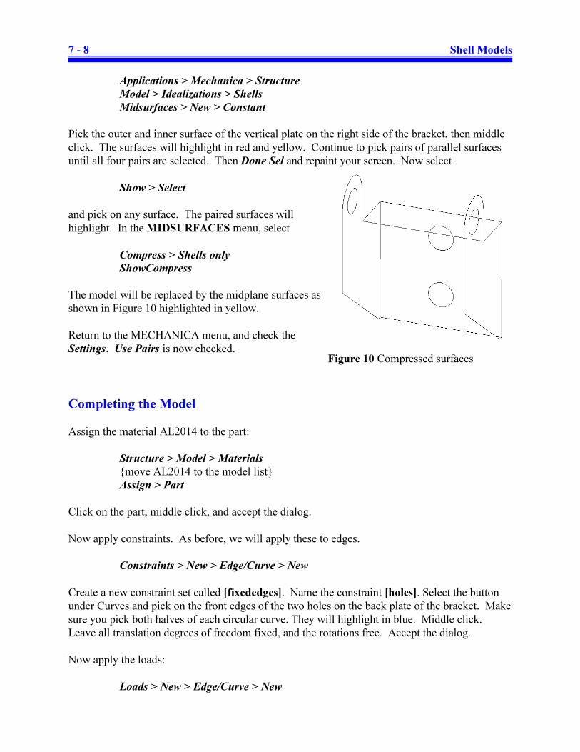
Completing the Model . . . . . . . . . . . . . . . . . . . . . . . . . . . . . . . . . . . . . . . . . . . . . . . . . . 7 - 8

Running the Model . . . . . . . . . . . . . . . . . . . . . . . . . . . . . . . . . . . . . . . . . . . . . . . . . . . . 7 - 10

Mixed Solids and Shells (Model #3) . . . . . . . . . . . . . . . . . . . . . . . . . . . . . . . . . . . . . . . . . . . 7 - 12

Creating the Shells . . . . . . . . . . . . . . . . . . . . . . . . . . . . . . . . . . . . . . . . . . . . . . . . . . . . 7 - 13

Defining the Constraints . . . . . . . . . . . . . . . . . . . . . . . . . . . . . . . . . . . . . . . . . . . . . . . . 7 - 15

Defining a Bearing Load . . . . . . . . . . . . . . . . . . . . . . . . . . . . . . . . . . . . . . . . . . . . . . . . 7 - 16

xi

Defining the Material . . . . . . . . . . . . . . . . . . . . . . . . . . . . . . . . . . . . . . . . . . . . . . . . . . 7 - 16

Running the Analysis . . . . . . . . . . . . . . . . . . . . . . . . . . . . . . . . . . . . . . . . . . . . . . . . . . 7 - 17

Reviewing the Results . . . . . . . . . . . . . . . . . . . . . . . . . . . . . . . . . . . . . . . . . . . . . . . . . . 7 - 17

Summary . . . . . . . . . . . . . . . . . . . . . . . . . . . . . . . . . . . . . . . . . . . . . . . . . . . . . . . . . . . . . . . . 7 - 18

Chapter 8 - Beams and Frames

Synopsis . . . . . . . . . . . . . . . . . . . . . . . . . . . . . . . . . . . . . . . . . . . . . . . . . . . . . . . . . . . . . . . . . . 8 - 1


Beam Coordinate Systems . . . . . . . . . . . . . . . . . . . . . . . . . . . . . . . . . . . . . . . . . . . . . . . . . . . . 8 - 1

The Beam Action Coordinate System BACS . . . . . . . . . . . . . . . . . . . . . . . . . . . . . . . . . 8 - 2

The Beam Shape Coordinate System BSCS . . . . . . . . . . . . . . . . . . . . . . . . . . . . . . . . . . 8 - 2

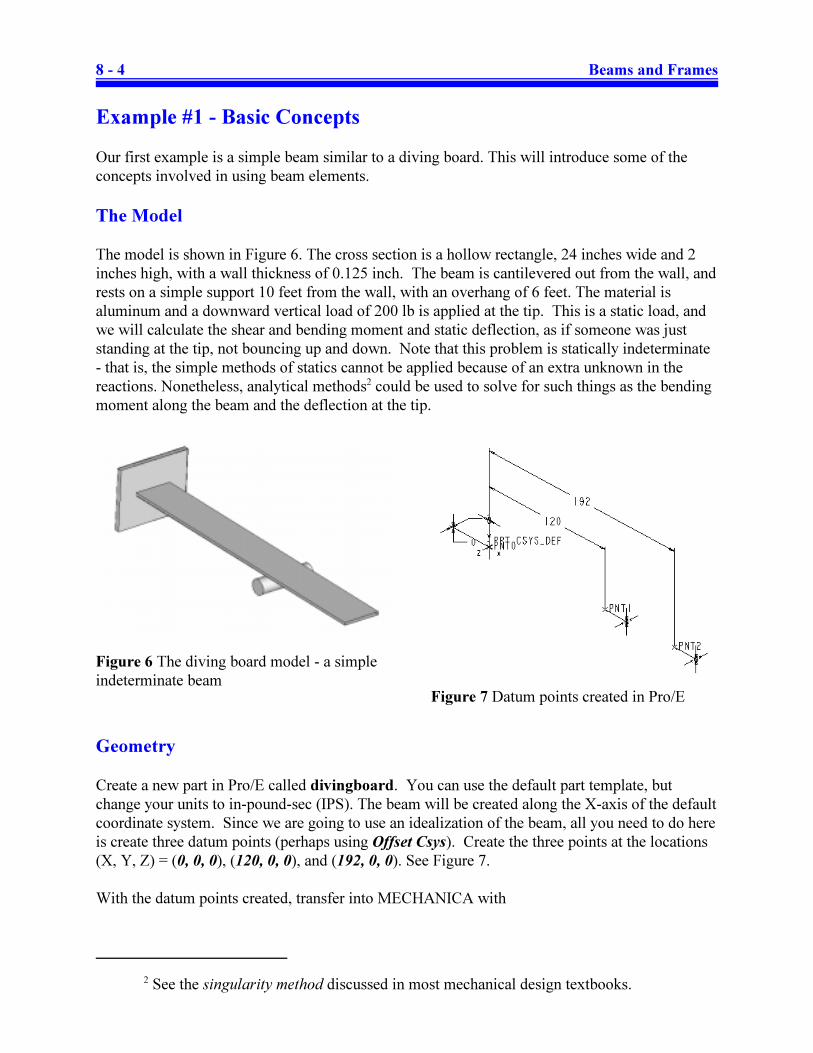
Example #1 - Basic Concepts . . . . . . . . . . . . . . . . . . . . . . . . . . . . . . . . . . . . . . . . . . . . . . . . . 8 - 4

The Model . . . . . . . . . . . . . . . . . . . . . . . . . . . . . . . . . . . . . . . . . . . . . . . . . . . . . . . . . . . . 8 - 4

Geometry . . . . . . . . . . . . . . . . . . . . . . . . . . . . . . . . . . . . . . . . . . . . . . . . . . . . . . . . . . . . . 8 - 4

Beam Elements . . . . . . . . . . . . . . . . . . . . . . . . . . . . . . . . . . . . . . . . . . . . . . . . . . . . . . . . 8 - 5

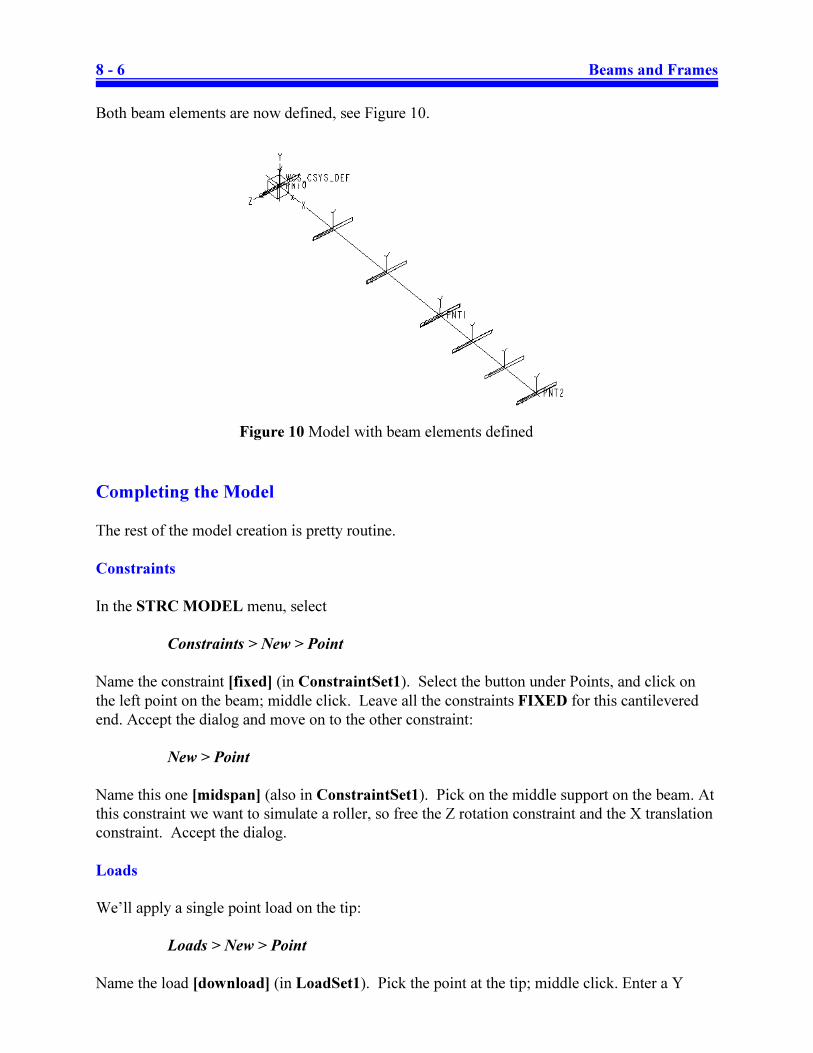
Completing the Model . . . . . . . . . . . . . . . . . . . . . . . . . . . . . . . . . . . . . . . . . . . . . . . . . . 8 - 6

Constraints . . . . . . . . . . . . . . . . . . . . . . . . . . . . . . . . . . . . . . . . . . . . . . . . . . . . . . . 8 - 6

Loads . . . . . . . . . . . . . . . . . . . . . . . . . . . . . . . . . . . . . . . . . . . . . . . . . . . . . . . . . . . 8 - 6

Analysis and Results . . . . . . . . . . . . . . . . . . . . . . . . . . . . . . . . . . . . . . . . . . . . . . . . . . . . 8 - 7

Deformation and Bending Stress . . . . . . . . . . . . . . . . . . . . . . . . . . . . . . . . . . . . . . 8 - 8

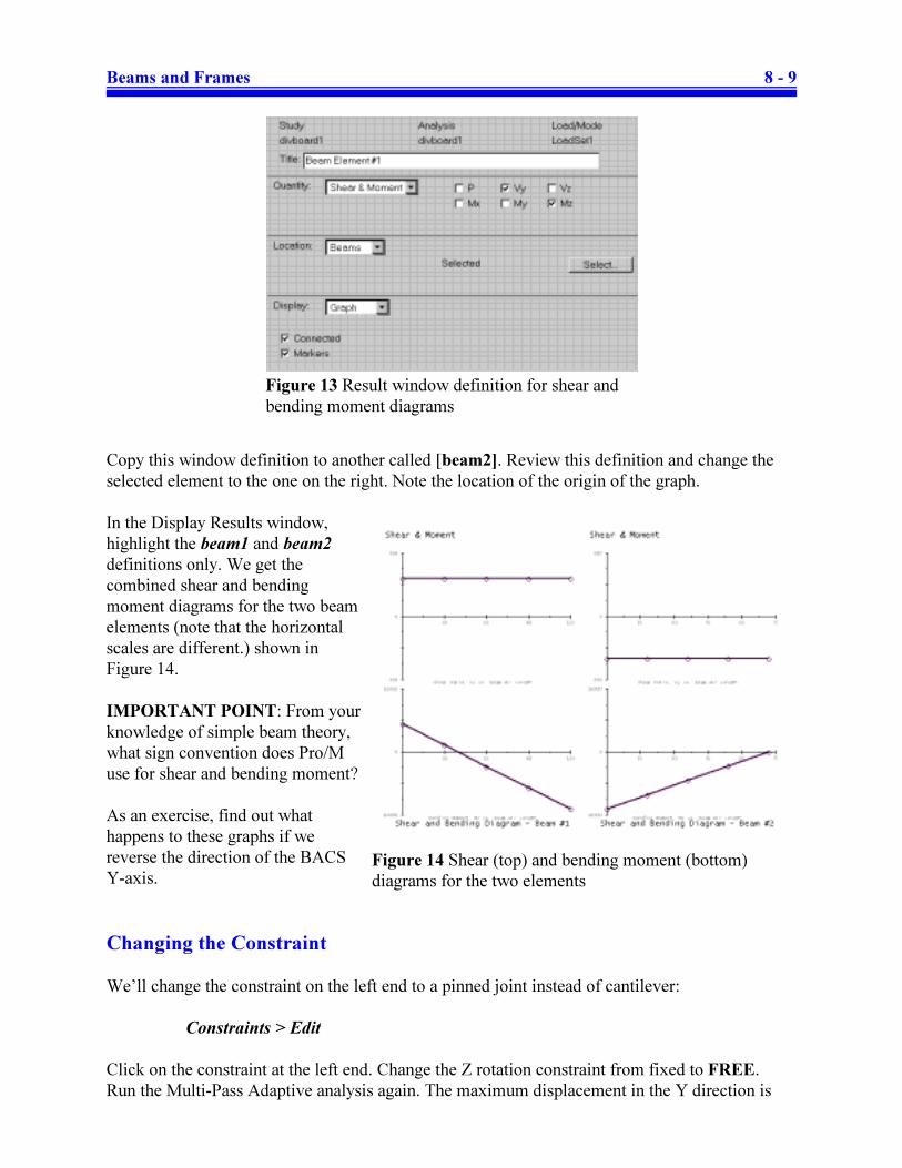
Shear and Moment Diagrams . . . . . . . . . . . . . . . . . . . . . . . . . . . . . . . . . . . . . . . . . 8 - 8

Changing the Constraint . . . . . . . . . . . . . . . . . . . . . . . . . . . . . . . . . . . . . . . . . . . . . . . . . 8 - 9

Example #2 - Distributed Loads, Beam Releases . . . . . . . . . . . . . . . . . . . . . . . . . . . . . . . . . 8 - 11

The Model . . . . . . . . . . . . . . . . . . . . . . . . . . . . . . . . . . . . . . . . . . . . . . . . . . . . . . . . . . . 8 - 11

Beam Geometry . . . . . . . . . . . . . . . . . . . . . . . . . . . . . . . . . . . . . . . . . . . . . . . . . . . . . . 8 - 11

Beam Elements . . . . . . . . . . . . . . . . . . . . . . . . . . . . . . . . . . . . . . . . . . . . . . . . . . . . . . . 8 - 12

Completing the Model . . . . . . . . . . . . . . . . . . . . . . . . . . . . . . . . . . . . . . . . . . . . . . . . . 8 - 13

Constraints . . . . . . . . . . . . . . . . . . . . . . . . . . . . . . . . . . . . . . . . . . . . . . . . . . . . . . 8 - 13

Distributed Loads . . . . . . . . . . . . . . . . . . . . . . . . . . . . . . . . . . . . . . . . . . . . . . . . . 8 - 13

Analysis and Results . . . . . . . . . . . . . . . . . . . . . . . . . . . . . . . . . . . . . . . . . . . . . . . . . . . 8 - 15

Result Windows . . . . . . . . . . . . . . . . . . . . . . . . . . . . . . . . . . . . . . . . . . . . . . . . . . 8 - 16

Beam Releases . . . . . . . . . . . . . . . . . . . . . . . . . . . . . . . . . . . . . . . . . . . . . . . . . . . . . . . 8 - 17

Setting Releases . . . . . . . . . . . . . . . . . . . . . . . . . . . . . . . . . . . . . . . . . . . . . . . . . . 8 - 17

Results . . . . . . . . . . . . . . . . . . . . . . . . . . . . . . . . . . . . . . . . . . . . . . . . . . . . . . . . . 8 - 18

Example #3 - Frames . . . . . . . . . . . . . . . . . . . . . . . . . . . . . . . . . . . . . . . . . . . . . . . . . . . . . . . 8 - 19

Model A - 2D Frame . . . . . . . . . . . . . . . . . . . . . . . . . . . . . . . . . . . . . . . . . . . . . . . . . . . 8 - 19

Model Geometry . . . . . . . . . . . . . . . . . . . . . . . . . . . . . . . . . . . . . . . . . . . . . . . . . 8 - 19

Beam Elements . . . . . . . . . . . . . . . . . . . . . . . . . . . . . . . . . . . . . . . . . . . . . . . . . . 8 - 20

Completing the Model . . . . . . . . . . . . . . . . . . . . . . . . . . . . . . . . . . . . . . . . . . . . . 8 - 21

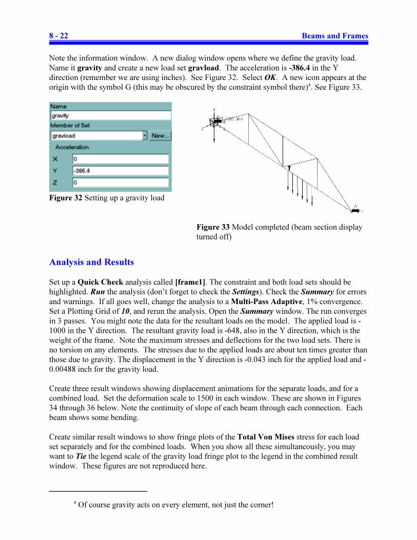
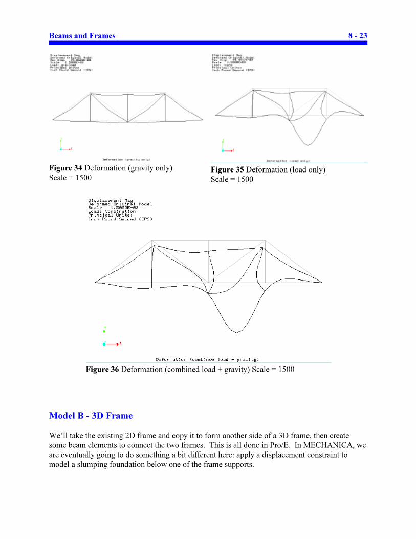
Analysis and Results . . . . . . . . . . . . . . . . . . . . . . . . . . . . . . . . . . . . . . . . . . . . . . 8 - 22

Model B - 3D Frame . . . . . . . . . . . . . . . . . . . . . . . . . . . . . . . . . . . . . . . . . . . . . . . . . . . 8 - 23

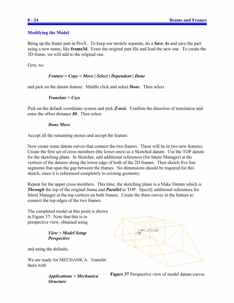
Modifying the Model . . . . . . . . . . . . . . . . . . . . . . . . . . . . . . . . . . . . . . . . . . . . . . 8 - 24

Creating Beam Elements . . . . . . . . . . . . . . . . . . . . . . . . . . . . . . . . . . . . . . . . . . . 8 - 25

Completing the Model . . . . . . . . . . . . . . . . . . . . . . . . . . . . . . . . . . . . . . . . . . . . . 8 - 25

Analysis and Results . . . . . . . . . . . . . . . . . . . . . . . . . . . . . . . . . . . . . . . . . . . . . . 8 - 26

xii

Displacement Constraint . . . . . . . . . . . . . . . . . . . . . . . . . . . . . . . . . . . . . . . . . . . 8 - 27

Summary . . . . . . . . . . . . . . . . . . . . . . . . . . . . . . . . . . . . . . . . . . . . . . . . . . . . . . . . . . . . . . . . 8 - 28

Chapter 9 - Miscellaneous Topics

Synopsis . . . . . . . . . . . . . . . . . . . . . . . . . . . . . . . . . . . . . . . . . . . . . . . . . . . . . . . . . . . . . . . . . . 9 - 1


Cyclic Symmetry . . . . . . . . . . . . . . . . . . . . . . . . . . . . . . . . . . . . . . . . . . . . . . . . . . . . . . . . . . . 9 - 1

Model Geometry . . . . . . . . . . . . . . . . . . . . . . . . . . . . . . . . . . . . . . . . . . . . . . . . . . . . . . . 9 - 2

Cyclic Constraints . . . . . . . . . . . . . . . . . . . . . . . . . . . . . . . . . . . . . . . . . . . . . . . . . . . . . . 9 - 3


Springs and Masses . . . . . . . . . . . . . . . . . . . . . . . . . . . . . . . . . . . . . . . . . . . . . . . . . . . . . . . . . 9 - 6

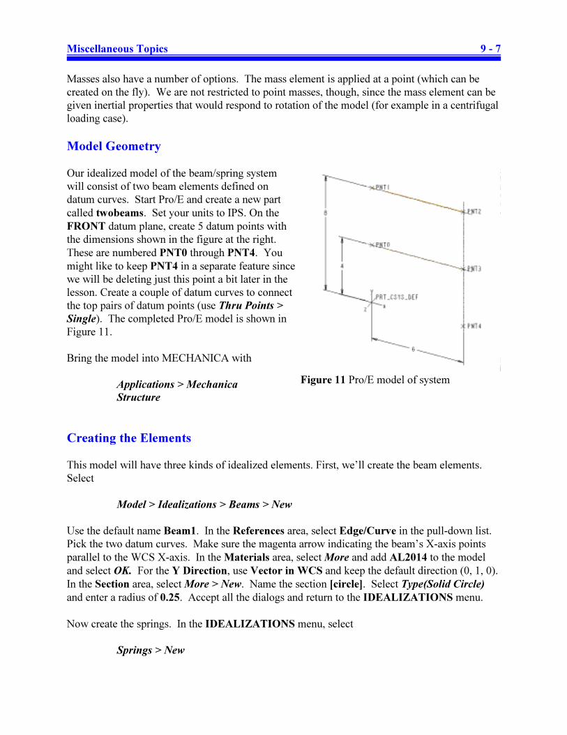
Model Geometry . . . . . . . . . . . . . . . . . . . . . . . . . . . . . . . . . . . . . . . . . . . . . . . . . . . . . . . 9 - 7

Creating the Elements . . . . . . . . . . . . . . . . . . . . . . . . . . . . . . . . . . . . . . . . . . . . . . . . . . . 9 - 7


Defining Measures . . . . . . . . . . . . . . . . . . . . . . . . . . . . . . . . . . . . . . . . . . . . . . . . . . . . . 9 - 9

Modal Analysis . . . . . . . . . . . . . . . . . . . . . . . . . . . . . . . . . . . . . . . . . . . . . . . . . . . . . . . . . . . 9 - 10

Setting up the Model . . . . . . . . . . . . . . . . . . . . . . . . . . . . . . . . . . . . . . . . . . . . . . . . . . . 9 - 11

Defining the Modal Analysis . . . . . . . . . . . . . . . . . . . . . . . . . . . . . . . . . . . . . . . . . . . . 9 - 11

Contact Analysis . . . . . . . . . . . . . . . . . . . . . . . . . . . . . . . . . . . . . . . . . . . . . . . . . . . . . . . . . . 9 - 13

Creating Contact Surfaces . . . . . . . . . . . . . . . . . . . . . . . . . . . . . . . . . . . . . . . . . . . . . . . 9 - 15

Summary . . . . . . . . . . . . . . . . . . . . . . . . . . . . . . . . . . . . . . . . . . . . . . . . . . . . . . . . . . . . . . . . 9 - 17

Conclusion . . . . . . . . . . . . . . . . . . . . . . . . . . . . . . . . . . . . . . . . . . . . . . . . . . . . . . . . . . . . . . . 9 - 17

Introduction 1 - 1

Chapter 1 :

Introduction to the Tutorials

Synopsis

An introduction to finite element analysis, with some cautions about its use and misuse;

examples of problems solved with MECHANICA; organization of the tutorials; tips and tricks

for using MECHANICA

Overview of this Lesson

‚ general comments about using Finite Element Analysis (FEA)

‚ examples of problems solved using Pro/MECHANICA Structure

‚ layout of the tutorials

‚ how the tutorial will present command sequences

‚ some tips and tricks for using MECHANICA

Finite Element Analysis

Finite Element Analysis (FEA), also known as the Finite Element Method (FEM), is probably the

most important tool added to the mechanical design engineer's toolkit this century. The

development of FEA has been driven by the desire for more accurate design computations in

more complex situations, allowing improvements in both the design procedure and products. The

growing use of FEA has been made possible by the creation of computation engines that are

capable of handling the immense volume of calculations necessary to prepare and carry out an

analysis and easily display the results for interpretation. With the advent of very powerful

desktop workstations, FEA is now available at a practical cost to virtually all engineers and

designers.

The Pro/MECHANICA software described in this introductory tutorial is only one of many

commercial systems that are available. All of these systems share many common capabilities. In

this tutorial, we will try to present both the commands for using MECHANICA and the reasons

behind those commands, so that the general procedures can be transferred to other FEA

packages. Notwithstanding this desire, it should be realized that Pro/M is unique in many ways

among packages currently available. Therefore, numerous topics treated will be specific to

Pro/M.

1 - 2 Introduction

1This refers to the problem of “convergence” whereby the FEA results must be verified or

tested so that they can be trusted. We will discuss convergence at some length later on and refer

to it continually throughout the manual.

Pro/MECHANICA (or Pro/M as we will call it) is actually a suite of three programs: Structure,

Thermal, and Motion. The first of these, Structure, is able to perform the following:

‚ linear static stress analysis

‚ modal analysis (mode shapes and natural frequencies)

‚ buckling analysis

‚ large deformation analysis (non-linear)

and others. This manual will be concerned only with the first two of these analyses. The

remaining types of problems are beyond the scope of an introductory manual. Once having

finished this manual, however, interested users should not find the other topics too difficult. The

other two programs (Thermal and Motion) are used for thermal analysis and dynamic analysis of

mechanical systems, respectively. Both of these programs can pass information (for example

temperature distributions) back to Structure in order to compute the associated stresses. In this

book, the use of Pro/M is meant to imply Structure only.

Pro/M offers much more than simply an FEA engine. We will see that Pro/M is really a design

tool since it will allow parametric studies as well as design optimization to be set up quite easily.

Moreover, unlike many other commercial FEM programs where determining accuracy can be

difficult or time consuming, Pro/M will be able to compute results with some certainty as to the

accuracy1.

Pro/M does not currently have the ability to handle non-linear problems, for example a stress

analysis problem involving a non-linearly elastic material like rubber. However, as of Release

2000i, problems involving very large geometric deflections can be treated, as long as the stresses

remain within the linearly elastic range for the material.

In this tutorial, we will concentrate on the main concepts and procedures for using the software

and focus on topics that seem to be most useful for new users and/or students doing design

projects and other course work. We assume that readers do not know anything about the

software, but are quite comfortable with Pro/Engineer. A short and very qualitative overview of

the FEA theoretical background has been included, but it should be emphasized that this is very

limited in scope. Our attention here is on the use and capabilities of the software, not providing a

complete course on using FEA, its theoretical origins, or the “art” of FEA modeling strategies.

For further study of these subjects, see the reference list at the end of the second chapter.

Examples of Problems Solved using MECHANICA

To give you a taste of what is to come, here are three examples of what you will be able to do

with MECHANICA on completion of these tutorials. The examples are a simple analysis, a

Introduction 1 - 3

2 The Von Mises stress is obtained by combining all the stress components at a point in a

way which produces a single value that can be compared to the yield strength of the material.

This is the most common way of examining the computed stress in a part.

Figure 1 Solid model of a part

Figure 2 Von Mises stress fringe plotFigure 3 Deformation of the part

parametric design study called a sensitivity analysis, and a design optimization. In

MECHANICA’s language, these are called design studies.

Example #1 : Analysis

This is the “bread and butter” type of problem for

MECHANICA. A model is defined by some geometry

(in 2D or 3D) in the geometry pre-processor,

Pro/Engineer. This is not as simple or transparent as

it sounds, as discussed below. The model is

transferred into Pro/Mechanica where material

properties are specified, loads and constraints are

applied, and one of several different types of analysis

can be run on the model. In the figure at the right, a

model of a somewhat crude connecting rod is shown.

This part is modeled using 3D solid elements. The

hole at the large end is fixed and a lateral bearing load

is applied to the inside surface of the hole at the other

end. The primary results are shown in Figures 2 and 3.

These are contours of the Von Mises stress2 on the part, shown in a fringe plot (these are, of

course, in color on the computer screen), and a wireframe view of the total (exaggerated)

deformation of the part (this can be shown as an animation). Here, we are usually interested in

the value and location of the maximum Von Mises stress in the part, whether the solution agrees

with our desired boundary conditions, and the magnitude and direction of deformation of the

part.

1 - 4 Introduction

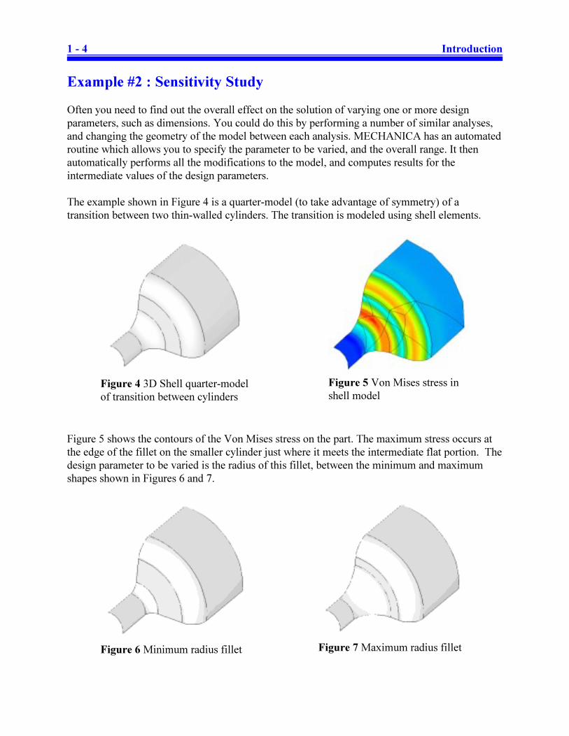
Figure 4 3D Shell quarter-model

of transition between cylinders

Figure 5 Von Mises stress in

shell model

Figure 6 Minimum radius fillet Figure 7 Maximum radius fillet

Example #2 : Sensitivity Study

Often you need to find out the overall effect on the solution of varying one or more design

parameters, such as dimensions. You could do this by performing a number of similar analyses,

and changing the geometry of the model between each analysis. MECHANICA has an automated

routine which allows you to specify the parameter to be varied, and the overall range. It then

automatically performs all the modifications to the model, and computes results for the

intermediate values of the design parameters.

The example shown in Figure 4 is a quarter-model (to take advantage of symmetry) of a

transition between two thin-walled cylinders. The transition is modeled using shell elements.

Figure 5 shows the contours of the Von Mises stress on the part. The maximum stress occurs at

the edge of the fillet on the smaller cylinder just where it meets the intermediate flat portion. The

design parameter to be varied is the radius of this fillet, between the minimum and maximum

shapes shown in Figures 6 and 7.

Introduction 1 - 5

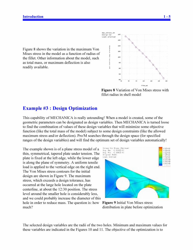
Figure 8 Variation of Von Mises stress with

fillet radius in shell model

Figure 9 Initial Von Mises stress

distribution in plate before optimization

Figure 8 shows the variation in the maximum Von

Mises stress in the model as a function of radius of

the fillet. Other information about the model, such

as total mass, or maximum deflection is also

readily available.

Example #3 : Design Optimization

This capability of MECHANICA is really astounding! When a model is created, some of the

geometric parameters can be designated as design variables. Then MECHANICA is turned loose

to find the combination of values of these design variables that will minimize some objective

function (like the total mass of the model) subject to some design constraints (like the allowed

maximum stress and/or deflection). Pro/M searches through the design space (for specified

ranges of the design variables) and will find the optimum set of design variables automatically!

The example shown is of a plane stress model of a

thin, symmetrical, tapered plate under tension. The

plate is fixed at the left edge, while the lower edge

is along the plane of symmetry. A uniform tensile

load is applied to the vertical edge on the right end.

The Von Mises stress contours for the initial

design are shown in Figure 9. The maximum

stress, which exceeds a design tolerance, has

occurred at the large hole located on the plate

centerline, at about the 12:30 position. The stress

level around the smaller hole is considerably less,

and we could probably increase the diameter of this

hole in order to reduce mass. The question is: how

much?

The selected design variables are the radii of the two holes. Minimum and maximum values for

these variables are indicated in the Figures 10 and 11. The objective of the optimization is to

1 - 6 Introduction

Figure 10 Minimum values of design

variables

Figure 11 Maximum values of design

variables

Figure 12 Optimization history: Von Mises stress (left) and total mass

(right)

minimize the total mass of the plate, while not exceeding a specified maximum stress.

Figure 12 shows a history of the design optimization computations. The figure on the left shows

the maximum Von Mises stress in the part that initially exceeds the allowed maximum stress, but

Pro/M very quickly adjusts the geometry to produce a design within the allowed stress. The

figure on the right shows the mass of the part. As the optimization proceeds, this is slowly

reduced until a minimum value is obtained (approximately 20% less than the original). Pro/M

allows you to view the shape change occurring at each iteration.

The final optimized design is shown in Figure 13. Notice the increased size of the interior hole,

and the more efficient use of material. The design limit stress now occurs on both holes.

Introduction 1 - 7

Figure 13 Von Mises stress distribution in

optimized plate

FEA User Beware!

Users of this (or any other FEA) software should be cautioned that, as in other areas of computer

applications, the GIGO (“Garbage In = Garbage Out”) principle applies. Users can easily be

misled into blind acceptance of the answers produced by the programs. Do not confuse pretty

graphs and pictures with correct modeling practice and accurate results.

A skilled practitioner of FEA must have a considerable amount of knowledge and experience.

The current state of sophistication of CAD and FEA software may lead non-wary users to

dangerous and/or disastrous conclusions. Users might take note of the fine print that

accompanies all FEA software licenses, which usually contains some text along these lines: “The

supplier of the software will take no responsibility for the results obtained . . .” and so on.

Clearly, the onus is on the user to bear the burden of responsibility for any conclusions that might

be reached from the FEA.

We might plot the situation something like Figure 14 on the next page. In order to intelligently

(and safely) use FEA, it is necessary to acquire some knowledge of the theory behind the method,

some facility with the available software, and a great deal of modeling experience. In this

manual, we assume that the reader's level of knowledge and experience with FEA initially places

them at the origin of the figure. The tutorial (particularly Chapter 2) will extend your knowledge

a little bit in the “theory” direction, at least so that we can know what the software requires for

input data, and (generally) how it computes the results. The step-by-step tutorials and exercises

will extend your knowledge in the “experience” direction. Primarily, however, this tutorial is

meant to extend your knowledge in the “FEA software” direction, as it applies to using

Pro/MECHANICA. Readers who have already moved out along the "theory" or "experience"

axes will have to bear with us - at least this manual should assist you in discovering the

1 - 8 Introduction

modeling experience

knowledge ofFEA software

knowledge ofFEA theory

Figure 14 Knowledge, skill, and experience requirements for FEA users

capabilities of the MECHANICA software package.

In summary, some quotes from speakers at an FEA panel at an ASME Computers in Engineering

conference in the early 1990's should be kept in mind:

"Don't confuse convenience with intelligence."In other words, as more powerful functions (such as automatic mesh generation) get

built in to FEA packages, do not assume that these will be suitable for every modeling

situation, or that they will always produce trustworthy results. If an option has

defaults, be aware of what they are and their significance to the model and the results

obtained. Above all, remember that just because it is easy, it is not necessarily right!

"Don't confuse speed with accuracy."Computers are getting faster and faster. This also means that they can compute an

inaccurate model faster than before - a wrong answer in half the time is hardly an

improvement!

and finally, the most important:

"FEA makes a good engineer better and a poor engineer dangerous."As our engineering tools get more sophisticated, there is a tendency to rely on them

more and more, sometimes to dangerous extremes. Relying solely on FEA for design

verification might be dangerous. Don’t forget your intuition, and remember that a lot

of very significant engineering design work has occurred over the years on the back of

an envelope. Let FEA become a tool that extends your design capability, not define it.

Introduction 1 - 9

Layout of this Manual

Running the Pro/MECHANICA software is not a trivial operation. However, with a little

practice, and learning only a fraction of the capabilities of the program, you can perform FEA of

reasonably complex problems. This manual is meant to guide you through the major features of

the software and how to use it. The manual is not meant to be a complete guide to either the

software or FEA modeling - consider it the elementary school of practical FEA!

Chapter 2 of the tutorial will present an overview of the theory and mathematics behind how

FEA is implemented in MECHANICA. In particular, the origin and differences between h-code

analysis and the p-code method in MECHANICA are discussed. The primary purpose of this

chapter is to outline the main capabilities of MECHANICA as they apply to the design and

analysis of mechanical parts. These include simple analyses, sensitivity studies, and parameter

optimization. This chapter will basically introduce you to the terminology used in the program,

and give you an overview of its operation.

Chapters 3 and 4 will present the basic procedure and commands for performing design studies

on solid models. This is a natural starting point, given that models imported from Pro/E are

usually solids. Common methods of displaying results are shown. Some issues of modeling are

discussed, such as symmetry. Several modeling pitfalls, which also occur in other model types

are investigated, and solutions proposed.

Chapter 5 will introduce you to the analysis of 2D models using idealizations. These are plane

stress and plane strain analyses. Geometry for these models is selected from the 3D part

geometry as created in Pro/E. The idealization, when applicable, results in a significant

reduction in the computational effort for the model.

The subject of Chapter 6 is axisymmetric models. These require that the geometry, loads, and

constraints can be based on a 2D layout that represents the problem.

Chapter 7 is devoted to a very important idealization - the shell model. Shells occur when the

model contains all or some thin-walled solid features. This idealization results in a greatly

reduced problem size and faster solution.

Beams and 2D and 3D frames (including trusses) are dealt with in Chapter 8. Both single

continuous beams and beams as components of frames are discussed. Beams can also be used in

combination with shells and solids.

Finally, Chapter 9 will deal with some miscellaneous topics including cyclic symmetry, spring

and mass elements, modal analysis, and contact analysis in assemblies.

At the end of each of these chapters, a number of additional exercises are presented. You should

try to do as many of these as you can in order to build up your knowledge and repertoire of

modeling scenarios.

1 - 10 Introduction

Tips for using MECHANICA

In the tutorial examples that follow, you will be lead through a number of simple problems

keystroke by keystroke. Each command will be explained in depth so that you will know the

“why” as well as the “what” and “how”. Resist the temptation to just follow the keystrokes - you

must think hard about what is going on in order to learn it. You should go through the tutorials

while working on a computer so that you experience the results of each command as it is entered.

Not much information will sink in if you just read the material. We have tried to capture exactly

the key-stroke, menu selection, or mouse click sequences to perform each analysis. These

actions are indicated in bold face italic type. Characters entered from the keyboard are enclosed

within square brackets. When more than one command is given in a sequence, they are separated

by the symbol ">". When several commands are entered on a single menu or window, they are

separated by the pipe symbol “ | ”. An option from a pull-down list will be indicated with the list

title and selected option in parantheses. So, for example, you might see command sequences

similar to the following:

Materials > Assign > Part > STEEL_IPS | Accept

Analysis (QuickCheck)

Results > Create > [VonMises] | Accept

At the end of each chapter in the manual, we have included some Questions for Review and

some simple Exercises which you should do. These have been designed to illustrate additional

capabilities of the software, some simple modeling concepts, and sometimes allow a comparison

with either analytical solutions or with alternative modeling methods. The more of these

exercises you do, the more confident you can be in setting up and solving your own problems.

Finally, here a few hints about using the software. Menu items and/or graphics entities on the

screen are selected by clicking on them with the left mouse button. We will often refer to this as a

‘left click’ or simply as a ‘click’. The middle mouse button (‘middle click’) can be used

(generally) whenever Accept, Enter, Close or Done is required. The dynamic view controls are

obtained by holding down the Ctrl key and dragging with a mouse button (left = zoom, middle =

spin, right = pan). Users of Pro/ENGINEER will be quite comfortable with these mouse controls.

Any menu commands grayed out are unavailable for the current context. Otherwise, any menu

item is available for use. You can, for example, jump from the design menus to the pulldown

menus at any time. Many operations can be launched by clicking and holding down the right

mouse button on an entry in the model tree or in the graphics window.

As of Release 2001, Pro/Engineer and Pro/Mechanica incorporate a new “object-action”

operating paradigm (as opposed to the previous “action-object” form). This means you can pick

an object on the screen (like a part surface), then specify the action to be performed on it (like

applying a load). This is a much more streamlined and natural sequence to process commands.

Of course, the previous action-object form will still work. In this Tutorial, command sequences

are represented at various times in either of the two forms. Hopefully, this will not get

confusing.

Introduction 1 - 11

So, with all that out of the way, let’s get started. The next chapter will give you an overview of

FEA theory, and how MECHANICA is different from other commercial packages.

FEM with MECHANICA 2 - 1

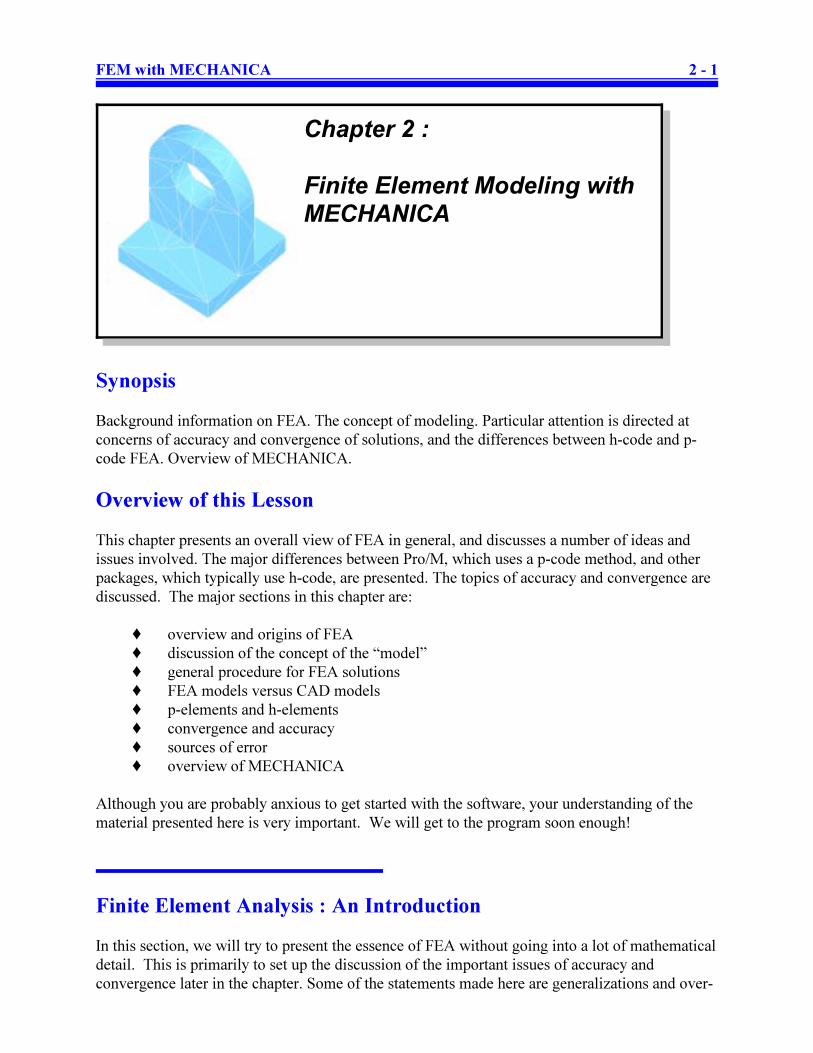
Chapter 2 :

Finite Element Modeling withMECHANICA

Synopsis

Background information on FEA. The concept of modeling. Particular attention is directed at

concerns of accuracy and convergence of solutions, and the differences between h-code and p-

code FEA. Overview of MECHANICA.


This chapter presents an overall view of FEA in general, and discusses a number of ideas and

issues involved. The major differences between Pro/M, which uses a p-code method, and other

packages, which typically use h-code, are presented. The topics of accuracy and convergence are

discussed. The major sections in this chapter are:

‚ overview and origins of FEA

‚ discussion of the concept of the “model”

‚ general procedure for FEA solutions

‚ FEA models versus CAD models

‚ p-elements and h-elements

‚ convergence and accuracy

‚ sources of error

‚ overview of MECHANICA

Although you are probably anxious to get started with the software, your understanding of the

material presented here is very important. We will get to the program soon enough!

Finite Element Analysis : An Introduction

In this section, we will try to present the essence of FEA without going into a lot of mathematical

detail. This is primarily to set up the discussion of the important issues of accuracy and

convergence later in the chapter. Some of the statements made here are generalizations and over-

2 - 2 FEM with MECHANICA

1 The PDE given represents the temperature within a solid body which is governed by the

conduction of heat within the body. There are no heat sources, and temperature on the boundary

of the body is known.

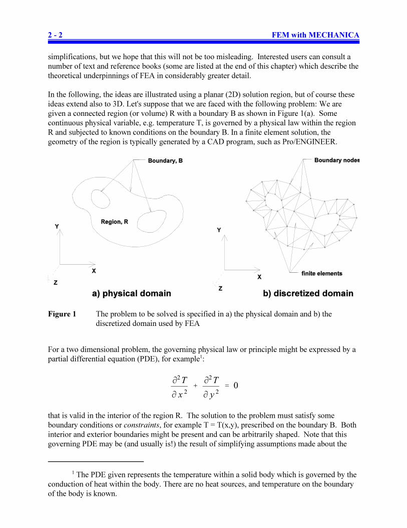
Figure 1 The problem to be solved is specified in a) the physical domain and b) the

discretized domain used by FEA

M2T

M x 2

%M2T

M y 2

' 0

simplifications, but we hope that this will not be too misleading. Interested users can consult a

number of text and reference books (some are listed at the end of this chapter) which describe the

theoretical underpinnings of FEA in considerably greater detail.

In the following, the ideas are illustrated using a planar (2D) solution region, but of course these

ideas extend also to 3D. Let's suppose that we are faced with the following problem: We are

given a connected region (or volume) R with a boundary B as shown in Figure 1(a). Some

continuous physical variable, e.g. temperature T, is governed by a physical law within the region

R and subjected to known conditions on the boundary B. In a finite element solution, the

geometry of the region is typically generated by a CAD program, such as Pro/ENGINEER.

For a two dimensional problem, the governing physical law or principle might be expressed by a

partial differential equation (PDE), for example1:

that is valid in the interior of the region R. The solution to the problem must satisfy some

boundary conditions or constraints, for example T = T(x,y), prescribed on the boundary B. Both

interior and exterior boundaries might be present and can be arbitrarily shaped. Note that this

governing PDE may be (and usually is!) the result of simplifying assumptions made about the


physical system, such as the material being homogeneous and isotropic, with constant linear

properties, and so on.

In order to analyze this problem, the region R is discretized into individual finite elements that

collectively approximate the shape of the region, as shown in Figure 1(b). This discretization is

accomplished by locating nodes along the boundary and in the interior of the region. The nodes

are then joined by lines to create the finite elements. In 2D problems, these can be triangles or

quadrilaterals; in 3D problems, the elements can be tetrahedra or 8-node "bricks". In some FEA

software, other higher order types of elements are also possible (e.g. hexagonal prisms). Some

higher order elements also have additional nodes along their edges. Collectively, the set of all

the elements is called a finite element mesh. In the early days of FEM, a great deal of effort was

required to set up the mesh. More recently, automatic meshing routines have been developed in

order to do most, if not all, of this tedious task.

In the FEA solution, values of the dependent variable (T, in our example) are computed only at

the nodes. The variation of the variable within each element is computed from the nodal values

so as to approximately satisfy the governing PDE. One way of doing this is by using

interpolating polynomials. In order for the PDE to be satisfied, the nodal values of each element

must satisfy a set of conditions represented by several linear algebraic equations usually

involving other nodal values.

The boundary conditions are implemented by specifying the values of the variables on the

boundary nodes. There is no guarantee that the true boundary conditions on the continuous

boundary B are satisfied between the nodes on the discretized boundary.

When all the individual elements in the mesh are combined, the discretization and interpolation

procedures result in a conversion of the problem from the solution of a continuous differential

equation into a very large set of simultaneous linear algebraic equations. This system can

typically have many thousands of equations in it, requiring special and efficient numerical

algorithms,. The solution of this algebraic system contains the nodal values that collectively

represent an approximation to the continuous solution of the initial PDE. An important issue,

then, is the accuracy of this approximation. In classical FEM solutions, the approximation

becomes more accurate as the mesh is refined with smaller elements. In the limit of zero mesh

size, requiring an infinite number of equations, the FEM solution to the PDE would be exact.

This is, of course, not achievable. So, a major issue revolves around the question “How fine a

mesh is required to produce answers of acceptable accuracy?” and the practical question is “Is it

feasible to compute this solution?” We will see a bit later how Pro/M solves these problems.

IMPORTANT POINT: In FEA stress analysis problems, the dependent variable in the

governing PDE's is the displacement from the reference (usually unloaded) position. The

material strain (displacement per unit length) is then computed from the displacement by

taking the derivative with respect to position. Finally, the stress components at any point in

the material are computed from the strain at that point. Thus, if the interpolating

polynomial for the spatial variation of the displacement field is linear within an element,

then the strain and stress will be constant within that element, since the derivative of a

linear function is a constant. The significance of this will be illustrated a bit later in this

lesson.


Figure 2 Developing a Model for Finite Element Analysis

The FEA Model and General Processing Steps

Throughout this manual, we will be using the term “model” extensively. We need to have a clear

idea of what we mean by the FEA model.

To get from the “real world” physical problem to the approximate FEA solution, we must go

through a number of simplifying steps. At each step, it is necessary to make decisions about what

assumptions or simplifications will be required in order to reach a final workable model. By

“workable”, we mean that the FEA model must allow us to compute the results of interest (for

example, the maximum stress in the material) with sufficient accuracy and with available time

and resources. It is no good building a model that is over-simplified to the point where it cannot

produce the results with sufficient accuracy. It is also no good producing a model that is “perfect”

but will not yield useful computational results for several weeks! Quite often, the FEA user must

compromise between the two extremes - accepting a slightly less accurate answer in a reasonable

solution time.

To arrive at a model suitable for FEA, we must go through the simplifying steps shown in Figure

2, as follows:

Real World º Simplified Physical Model

This simplification step involves making assumptions about physical properties or the physical

layout and geometry of the problem. For example, we usually assume that materials are

homogeneous and isotropic and free of internal defects or flaws. It is also common to ignore

aspects of the geometry that will have no (anticipated) effect on the results, such as the

chamfered and filleted edges on the bracket shown in Figure 3, and perhaps even the mounting


Figure 3 The “Real World” Object

Figure 4 The idealized physical

model

Figure 5 A mesh of solid brick

elements

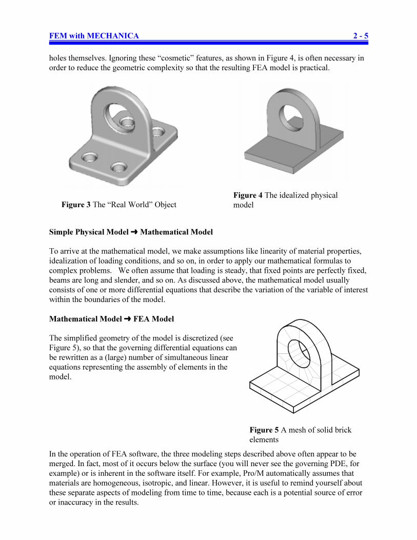
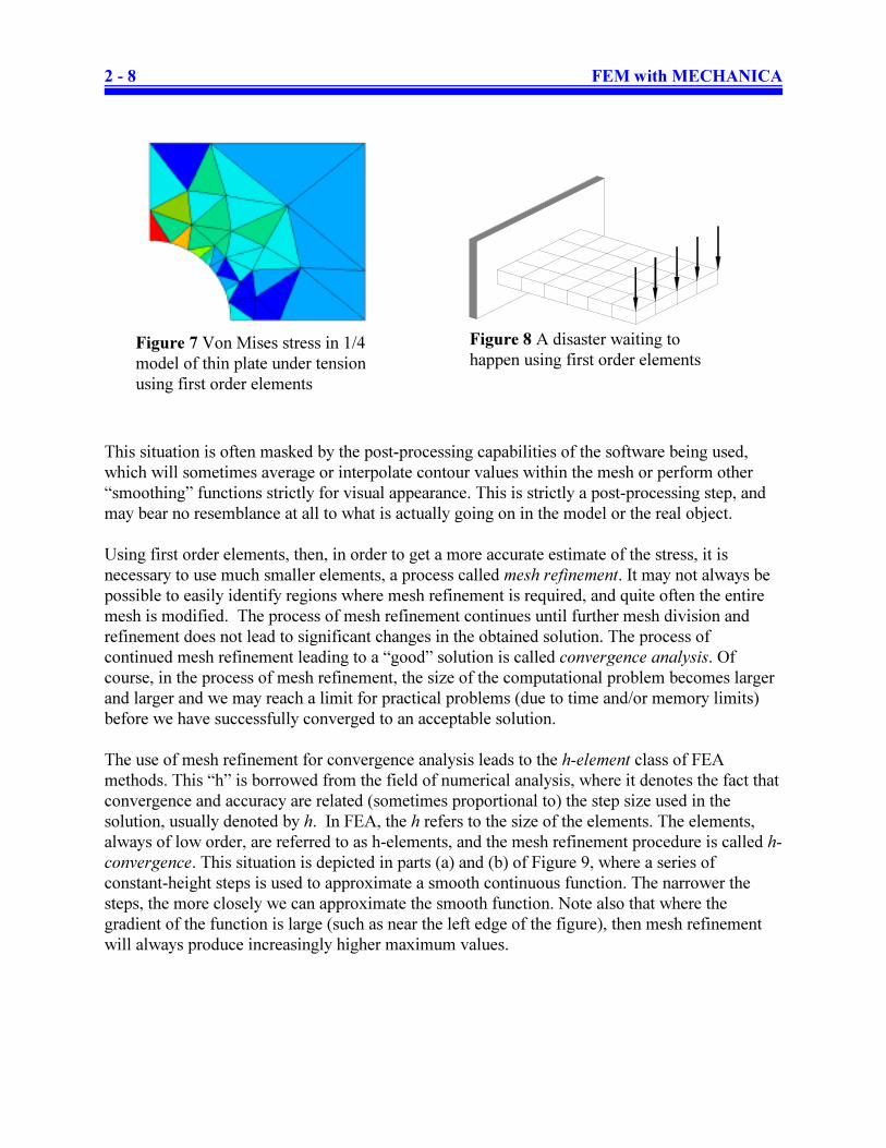
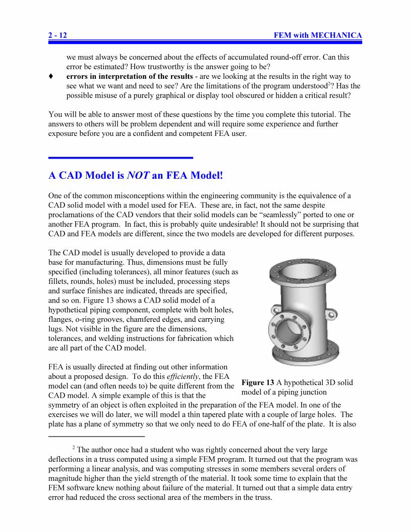
holes themselves. Ignoring these “cosmetic” features, as shown in Figure 4, is often necessary in

order to reduce the geometric complexity so that the resulting FEA model is practical.

Simple Physical Model º Mathematical Model

To arrive at the mathematical model, we make assumptions like linearity of material properties,

idealization of loading conditions, and so on, in order to apply our mathematical formulas to

complex problems. We often assume that loading is steady, that fixed points are perfectly fixed,

beams are long and slender, and so on. As discussed above, the mathematical model usually

consists of one or more differential equations that describe the variation of the variable of interest

within the boundaries of the model.

Mathematical Model º FEA Model

The simplified geometry of the model is discretized (see

Figure 5), so that the governing differential equations can

be rewritten as a (large) number of simultaneous linear

equations representing the assembly of elements in the

model.

In the operation of FEA software, the three modeling steps described above often appear to be

merged. In fact, most of it occurs below the surface (you will never see the governing PDE, for

example) or is inherent in the software itself. For example, Pro/M automatically assumes that

materials are homogeneous, isotropic, and linear. However, it is useful to remind yourself about

these separate aspects of modeling from time to time, because each is a potential source of error

or inaccuracy in the results.


Create Geometrywith Pro/E

Model Type

Simulation Parameters:- material properties- model constraints

- applied loads

Discretize Modelto Form

Finite Element Mesh

Set up andSolve Linear System

Compute/DisplayResults of Interest

Review

Pro/MECHANICA

"RUN"

Figure 6 Overall steps in FEA Solution

Steps in Preparing an FEA Model for Solution

Starting from the simplified geometric model, there are generally several steps to be followed in

the analysis. These are:

1. identify the model type

2. specify the material properties, model constraints, and applied loads

3. discretize the geometry to produce a finite element mesh

4. solve the system of linear equations

5. compute items of interest from the solution variables

6. display and critically review results and, if necessary, repeat the analysis

The overall procedure is illustrated in

Figure 6. Some additional detail on each of

these steps is given below. The major steps

must be executed in order, and each must

be done correctly before proceeding to the

next step. When a problem is to be re-

analyzed (for example, if a stress analysis is

to be performed for the same geometry but

different loads), it will not usually be

necessary to return all the way to the

beginning. The available re-entry points

will become clear as you move through

these tutorials.

The steps shown in the figure are:

1. The geometric model of the

part/system is created using

Pro/ENGINEER.

2. On entry to Pro/M, the model type

must be identified. The default is a

solid model.

3. A) Specify material properties for

the model. It is not necessary that all the elements have the same properties. In an

assembly, for example, different parts can be made of different materials. For stress

analysis the required properties are Young’s modulus and Poisson’s ratio. Most FEA

packages contain built-in libraries containing properties of common materials (steel,

iron, aluminum, etc.).

B) Identify the constraints on the solution. In stress analysis, these could be fixed points,

points of specified displacement, or points free to move in specified directions only.

C) Specify the applied loads on the model (point loads, uniform edge loads, pressure on

surfaces, etc.).


4. Once you are satisfied with your model, you set up and run a processor that actually

performs the solution to the posed FEA problem. This starts with the automatic creation of

the finite element mesh from the geometric model by a subprogram within Pro/M called

AutoGEM. Pro/M will trap some modeling errors here. The processor will produce a

summary file of output messages which can be consulted if something goes wrong - for

example, a model that is not sufficiently constrained by boundary conditions.

5. FEA produces immense volumes of output data. The only feasible way of examining this is

graphically. Pro/M has very powerful graphics capabilities to examine the results of the

FEA - displaced shape, stress distributions, mode shapes, etc. Hard copy of the results file

and screen display is easy to obtain.

6. Finally, the results must be reviewed critically. In the first instance, the results should agree

with our modeling intent. For example, if we look at an animated view of the deformation,

we can easily see if our boundary constraints have been implemented properly. The results

should also satisfy our intuition about the solution (stress concentration around a hole, for

example). If there is any cause for concern, it may be advisable to revisit some aspects of

the model and perform the analysis again.

P-Elements versus H-Elements

Not all discretized finite elements are created equal! Here is where a major difference arises

between MECHANICA and most other FEA programs.

Convergence of H-elements (the “classic” approach)

Following the classic approach, other programs often use low order interpolating polynomials in

each element. This has significant ramifications, especially in stress analysis. As mentioned

above, in stress analysis the primary solution variables are the displacements of the nodes. The

interpolating functions are typically linear (first order) within each element. Strain is obtained by

taking the derivatives of the displacement field and the stress is computed from the material

strain. For a first order interpolating polynomial within the element, this means that the strain and

therefore the stress components within the element are constant everywhere. The situation is

depicted in Figure 7, which shows the computed Von Mises stress in each of the elements

surrounding a hole in a thin plate under tension. Such discontinuity in the stress field between

elements is, of course, unrealistic and will lead to inaccurate values for the maximum stress.

Low order elements lead to the greatest inaccuracy precisely in the regions of greatest interest,

typically where there are large gradients within the real object.

An even more disastrous situation is shown in Figure 8. This is a solid cantilever beam with a

uniform transverse load modeled using solid brick elements. With only a single first-order

element through the thickness, the computed stress will be the same on the top and bottom of the

beam. This is clearly wrong, yet the FEA literature and product demonstrations abound with

examples similar to this.


Figure 7 Von Mises stress in 1/4

model of thin plate under tension

using first order elements

Figure 8 A disaster waiting to

happen using first order elements

This situation is often masked by the post-processing capabilities of the software being used,

which will sometimes average or interpolate contour values within the mesh or perform other

“smoothing” functions strictly for visual appearance. This is strictly a post-processing step, and

may bear no resemblance at all to what is actually going on in the model or the real object.

Using first order elements, then, in order to get a more accurate estimate of the stress, it is

necessary to use much smaller elements, a process called mesh refinement. It may not always be

possible to easily identify regions where mesh refinement is required, and quite often the entire

mesh is modified. The process of mesh refinement continues until further mesh division and

refinement does not lead to significant changes in the obtained solution. The process of

continued mesh refinement leading to a “good” solution is called convergence analysis. Of

course, in the process of mesh refinement, the size of the computational problem becomes larger

and larger and we may reach a limit for practical problems (due to time and/or memory limits)

before we have successfully converged to an acceptable solution.

The use of mesh refinement for convergence analysis leads to the h-element class of FEA

methods. This “h” is borrowed from the field of numerical analysis, where it denotes the fact that

convergence and accuracy are related (sometimes proportional to) the step size used in the

solution, usually denoted by h. In FEA, the h refers to the size of the elements. The elements,

always of low order, are referred to as h-elements, and the mesh refinement procedure is called h-

convergence. This situation is depicted in parts (a) and (b) of Figure 9, where a series of

constant-height steps is used to approximate a smooth continuous function. The narrower the

steps, the more closely we can approximate the smooth function. Note also that where the

gradient of the function is large (such as near the left edge of the figure), then mesh refinement

will always produce increasingly higher maximum values.


(c) second order element leads to linear stress variation within each element

(d) higher order element will reduce error even further without changing the element size

(a) first order elements lead to constant stress within each element

h

(b) error is reduced by reducing the element size O(h)

h / 2

Figure 9 Approximation of stress function in a model

The major outcome of using h-elements is the need for meshes of relatively small elements.

Furthermore, h-elements are not very tolerant of shape extremes in terms of skewness, rapid size

variation through the mesh, large aspect ratio, and so on. This further increases the number of

elements required for an acceptable mesh, and this, of course, greatly increases the computational

cost of the solution.

Convergence of P-elements (the Pro/MECHANICA approach)

Now, the major difference incorporated in MECHANICA is the following: instead of constantly

refining and recreating finer and finer meshes, convergence is obtained by increasing the order of

the interpolating polynomials on each element. The mesh stays the same for every iteration,

called a p-loop pass. The use of higher order interpolating polynomials for convergence analysis

leads to the p-element class of FEA methods, where the “p” denotes polynomial. This method is

depicted in parts (c) and (d) of the Figure 9. Only elements in regions of high gradients are

bumped up to higher order polynomials. Furthermore, by examining the effects of going to

higher order polynomials, MECHANICA can monitor the expected error in the solution, and

automatically increase the polynomial order only on those elements were it is required. Thus, the

convergence analysis is performed quite automatically, with the solution proceeding until an

accuracy limit (set by the user) has been satisfied. With MECHANICA, the limit for the

polynomial order is 9. In theory, it would be possible to go to higher orders than this, but the

computational cost starts to rise too quickly. If the solution cannot converge even with these 9th


Figure 10 A mesh of solid tetrahedral (4

node) h-elements Figure 11 A mesh of tetrahedral p-elements

produced by MECHANICA.

order polynomials, it may be necessary to recreate the mesh at a slightly higher density so that

lower order polynomials will be sufficient. This is a very rare occurrence.

The use of p-elements has a number of features/advantages:

< The same mesh can be used throughout the convergence analysis, rather than

recreating meshes or local mesh refinement required by h-codes.

< The mesh is virtually always more coarse and contains fewer elements than h-codes.

Compare the meshes in Figures 10 and 11, and note that the mesh of h-elements in

Figure 10 would probably not produce very good results, depending on the loads and

constraints applied. The reduced number of elements in Pro/M (which can be a

couple of orders of magnitude smaller) initially reduces the computational load, but as

the order of the polynomials gets higher, this advantage is somewhat diminished.

< The restrictions on element size and shape are not nearly as stringent for p-elements

as they are for h-elements (where concerns of aspect ratio, skewness, and so on often

arise).

< Automatic mesh generators, which can produce very poor meshes for h-elements, are

much more effective with p-elements, due to the reduced requirements and limitations

on mesh geometry.

< Since the same mesh is used throughout the analysis, this mesh can be tied directly to

the geometry. This is the key reason why MECHANICA is able to perform sensitivity

and optimization studies during which the geometric parameters of a body can

change, but the program does not need to be constantly re-meshing the part.

Convergence and Accuracy in the Solution

It should be apparent that, due to the number of simplifying assumptions necessary to obtain

results with FEA, we should be quite cautious about the results obtained. No FEA solution


Figure 12 Two common convergence measures

using p-elements.

should be accepted unless the convergence properties have been examined.

For h-elements, this generally means doing the problem several times with successively smaller

elements and monitoring the change in the solutions. When decreasing the element size results

in a negligible (or acceptably small) change in the solution, then we are generally satisfied that

the FEA has wrung all the information out of the model that it can.

As mentioned above, with p-elements, the

convergence analysis is built in to the

program. Since the geometry of the mesh

does not change, no remeshing is required.

Rather, each successive solution (called a

p-loop pass) is performed with increasing

orders of polynomials (only on elements

where this is required) until the change

between iterations is “small enough”.

Figure 12 shows the convergence behavior

of two common measures used to monitor

convergence in MECHANICA. These are

the maximum Von Mises stress and the

total strain energy. Note that the Von Mises

stress will generally always increase during

the convergence test, but can behave quite

erratically as we will see later. Because

Von Mises stress is a local measure, the

strain energy is probably a better measure

to use to control convergence.

Sources of Error

Error enters into the FEA process in a number of ways:

‚ errors in problem definition - are the geometry, loads, and constraints known and

implemented accurately? Is the correct analysis being performed? Are the material

properties correct and/or appropriate?

‚ errors in creating the physical model - can we really use symmetry? Is the material

isotropic and homogeneous, as assumed? Are the physical constants known? Does the

material behave linearly?

‚ errors in creating the mathematical model - is the model complete enough to capture the

effects we wish to observe? Is the model overly complex? Does the mathematical model

correctly express the physics of the problem?

‚ errors in discretization - is the mesh too coarse or too fine? Have we left accidental

“holes” in the model? If using shell elements, are there tears or rips (free edges) between

elements where there shouldn’t be?

‚ errors in the numerical solution - when dealing with very large computational problems,


2 The author once had a student who was rightly concerned about the very large

deflections in a truss computed using a simple FEM program. It turned out that the program was

performing a linear analysis, and was computing stresses in some members several orders of

magnitude higher than the yield strength of the material. It took some time to explain that the

FEM software knew nothing about failure of the material. It turned out that a simple data entry

error had reduced the cross sectional area of the members in the truss.

Figure 13 A hypothetical 3D solid

model of a piping junction

we must always be concerned about the effects of accumulated round-off error. Can this

error be estimated? How trustworthy is the answer going to be?

‚ errors in interpretation of the results - are we looking at the results in the right way to

see what we want and need to see? Are the limitations of the program understood2? Has the

possible misuse of a purely graphical or display tool obscured or hidden a critical result?

You will be able to answer most of these questions by the time you complete this tutorial. The

answers to others will be problem dependent and will require some experience and further

exposure before you are a confident and competent FEA user.

A CAD Model is NOT an FEA Model!

One of the common misconceptions within the engineering community is the equivalence of a

CAD solid model with a model used for FEA. These are, in fact, not the same despite

proclamations of the CAD vendors that their solid models can be “seamlessly” ported to one or

another FEA program. In fact, this is probably quite undesirable! It should not be surprising that

CAD and FEA models are different, since the two models are developed for different purposes.

The CAD model is usually developed to provide a data

base for manufacturing. Thus, dimensions must be fully

specified (including tolerances), all minor features (such as

fillets, rounds, holes) must be included, processing steps

and surface finishes are indicated, threads are specified,

and so on. Figure 13 shows a CAD solid model of a

hypothetical piping component, complete with bolt holes,

flanges, o-ring grooves, chamfered edges, and carrying

lugs. Not visible in the figure are the dimensions,

tolerances, and welding instructions for fabrication which

are all part of the CAD model.

FEA is usually directed at finding out other information

about a proposed design. To do this efficiently, the FEA

model can (and often needs to) be quite different from the

CAD model. A simple example of this is that the

symmetry of an object is often exploited in the preparation of the FEA model. In one of the

exercises we will do later, we will model a thin tapered plate with a couple of large holes. The

plate has a plane of symmetry so that we only need to do FEA of one-half of the plate. It is also


Figure 14 The 3D solid model of

pipe junction

Figure 15 Shell elements of

specified thickness created from 3D

model

Figure 16 Von Mises stress in the

FEA model

quite common in FEA to ignore minor features like

rounds, fillets, chamfers, holes, minor changes in surface

profile, and other cosmetic features unless these features

will have a large effect on the measures of interest in the

model. Most frequently, they do not, and can be ignored.

Figure 14 shows an FEA model of the piping component

created to determine the maximum Von Mises stress in the

vicinity of the filleted connection between the two pipes.

The differences between the two models shown in Figures

13 and 14 are immediately obvious. Figures 15 and 16

show the mesh of shell elements created from the surface,

and the computed Von Mises stress.

In summary, the stated goal of FEA (the “Golden Rule”, if you like) might be expressed as:

Use the simplest model possible that will yield sufficiently reliable

results of interest at the lowest computational cost.

You can easily see how this might be at odds with the requirements of a CAD model. For further

discussion of this, see the excellent book Building Better Products with Finite Element

Analysis by Vince Adams and Abraham Askenazi, Onword Press, 1998.


Overview of Pro/MECHANICA Structure

Basic Operation

We are going to start using Pro/M in the next chapter. Before we dive in, it will be useful to have

an overall look at the function and organization of the software. This will help to explain some of

the Pro/M terminology and see how the program relates to the ideas presented in this chapter’s

overview of FEA.

We can divide the operation and functionality of Pro/M Structure according to the rows in Table

I below. These entries are further elaborated in the next few pages. In the process of setting up

and running a solution, you will basically need to pick one option from each row in the table. The

top-down organization of the table is roughly in the order that these decisions must be made.

Other issues such as creation of the model geometry and post-processing and display of final

results will be left to subsequent chapters.

TABLE I - An Overall View of Pro/M Capability and Function

MECHANICA

Options

Description

Mode of

Operation

Independent

Integrated

how Pro/M is operated with respect to

Pro/ENGINEER

Type of Model 3D

Plane Stress

Plane Strain

Axisymmetric

basic structure of the model

Type of

Elements

Shell

Beam

Solid

Spring

Mass

element types that can be used in a model

Analysis

Methods

Static

Modal

Buckling

Pre-stress modal

Pre-stress buckling

the fundamental solution being sought for the

model

Convergence

Methods

Quick Check

Single Pass Adaptive

Multi-Pass Adaptive

method of monitoring convergence in the

solution

Design Studies Standard

Sensitivity

Optimization

high level methods to organize essentially

repetitive computations


3 A third mode, called linked, was available up until Release 2000i, but has been

removed.

Modes of Operation

A discussion of the full details of operating modes gets pretty confusing, so only the main points

are presented here. These are:

1. Pro/M can operate in two modes3, in relation to its cousin application Pro/ENGINEER.

These are: independent and integrated. A special license is required to run the

independent version. In the student edition, only integrated mode is possible.

2. The user interface is determined by the mode:

‚ integrated mode - Pro/ENGINEER interface

‚ independent mode - Pro/MECHANICA interface

3. If you start out in Pro/ENGINEER to create the part (or assembly) geometry and call up

MECHANICA, you will initially be running in integrated mode. You can then switch to

independent mode if desired (and if your license allows it), as illustrated here (note that the

arrow is a one-way transfer - you can’t get back again!):

Integrated º Independent

Mode Mode

4. If you switch to independent mode, the connection with Pro/ENGINEER will be severed.

Any changes in design parameters (for example following an optimization) must be

manually transferred back into the Pro/E model.

5. In integrated mode, a few Pro/M commands and result displays are not available. However

the tight integration with Pro/E makes it very easy to perform design modification and

quick FEA.

6. In integrated mode, the user interface is the same as Pro/E. Only one set of controls to

learn! The independent mode user interface is quite different.

7. The full set of Pro/M commands and functions are available in independent mode (for

example: display of some types of results such as element p-levels, manual and semi-

automatic mesh generation for difficult models).

8. Although independent mode gives access to the complete range of MECHANICA

functionality, the benefits of feature-based geometry creation/modification are lost.

A condensed comparison of these operating modes is shown in Table II on the next page. As

mentioned above, all the tutorials in this manual are meant to be run in integrated mode.


TABLE II - Pro/MECHANICA Modes of Operation

Integrated Mode Independent Mode

Pro/E interface Pro/M interface

all analyses available all analyses available

2D and 3D models 2D and 3D models

some measures of results not available all measures available

some analysis options not available

(eg excluding elements)

all options available

all elements generated automatically element creation manual or automatic

sensitivity and optimization using

Pro/E parameters only

sensitivity and optimization uses Pro/M

variables

Types of Models

This is fairly self-explanatory. In addition to 3D solid, shell, and beam models, Pro/M in both

modes can treat 2D models (plane stress, plane strain, or axisymmetric). Note that all geometry

and model entities (loads and constraints) for all 2D model types must be defined in the XY

plane of a selected coordinate system. Also, a very thin plate might be modeled as a 2D shell,

but if it is loaded with any force components normal to the plate, then it becomes a 3D problem.

Independent Pro/M contains a good set of tools to create both 2D and 3D geometry.

Complicated 3D geometry of parts would be easier to make in Pro/E or some other CAD

package, and brought into Pro/M in integrated mode. The model geometry is generally created

entirely in Pro/E. It is possible to create some (non-solid) simulation features while in Pro/M,

such as datum points and curves.

Types of Elements

The various types of elements that can be used in Pro/M are listed in Table I. It is possible to use

different types of elements in the same model (e.g. combining solid + beam + spring elements),

but we will discuss only a couple of models of this degree of complexity in these tutorials. At

first glance, this seems like a limited list of element types. H-element programs typically have

large libraries of different element types, but these are often necessary to overcome the

limitations of low order simple h-elements. In Pro/M, we do not have this problem and you can

do practically anything with the elements available.


Analysis Methods

For a given model, several different analysis types are possible. For example, the static analysis

will compute the stresses and deformations within the model, while the modal analysis will

compute the mode shapes and natural frequencies. Buckling analysis will compute the buckling

loads on the body, and so. Other analysis methods are available but in this manual, we will only

look at static stress and modal analysis.

Convergence Methods

As discussed above, using the p-code method allows Pro/M to monitor the solution and modify

the polynomial edge order until a solution has been achieved to a specified accuracy. This is

implemented with three options:

# Quick Check - This actually isn’t a convergence method since the model is run only for a

single fixed (low, usually 3) polynomial order. The results of a Quick Check should

never be trusted. What a Quick Check is for is to quickly run the model through the solver

in order to pick up any errors that may have been made, for example in the constraints. A

quick review of the results will also indicate whether any gross modeling errors have been

made and possibly to point out potential problem areas in the model.

# Single Pass Adaptive - More than a Quick Check, but less than a complete convergence

run, the single pass adaptive method performs one pass at a low polynomial order, assesses

the accuracy of the solution, modifies the p-level of “problem elements”, and does a final

pass with some elements raised to an order that should provide reasonable results. Unless

the model is very computationally intensive and/or is very well behaved and understood,

avoid this method. The Single Pass Adaptive analysis is available for most model types.

# Multi-Pass Adaptive - The ultimate in convergence analysis. Multiple “p-loop” passes are

made through the solver, with edge orders of “problem elements” being increased with each

pass. This iterative approach continues until either the solution converges to a specified

accuracy or the maximum specified edge order (default 6, maximum 9) is reached. At the

conclusion of the run, the convergence measures may be examined. These are typically the

Von Mises stress and the total strain energy, as shown in Figure 12. Unless you have a very

good reason not to, always base your final conclusions on the results obtained using this

convergence method.

Design Studies

A Design Study is a problem or set of problems that you define for a particular model. When you

ultimately press the Run button on Pro/M, what will execute is a design study - it is the top-most

level of organization in Pro/M. There are three types of design studies:

# A Standard design study is the most basic and simple. It will include at least one but

possibly several analyses (for example a static analysis plus a modal analysis). For this


study, you need to specify the geometry, create the elements, assign material properties, set

up loads and constraints, determine the analysis and convergence types, and then display

and review the final results. The Standard design study is what most people would consider

“Finite Element Analysis.”

# A sensitivity design study can be set up so that results are computed for several different

values of designated design variables or material properties. In addition to the standard

model, you need to designate the design variables and the range over which you want them

to vary. You can use a sensitivity study to determine, for example, which design variables

will have the most effect on a particular measure of performance of the design like the

maximum stress or total mass.

# Finally, the most powerful design study is an optimization. For this, you start with a basic

FEA model. You then specify a desired goal (such as minimum mass of the body),

geometric constraints (such as dimensions or locations of geometric entities), material

constraints (such as maximum allowed stress) and one or more design variables which can

vary over specified ranges. Pro/M will then search through the space of the design variables

and determine the best design that satisfies your constraints. Amazing!

A Brief Note about Units

It is crucial to use a consistent set of units throughout your Pro/M activities. The program itself

has no default set of units (other than those brought in with the model from Pro/E), and only uses

the numerical values provided by you. Thus, if your geometry is created with a particular linear

unit like mm or inches in mind, you must make sure that any other data supplied, such as loads

(force, pressure) and material properties (density, Young’s modulus, and so on) are defined

consistently. The built-in material libraries offer properties for common materials in four sets of

units (all at room temperature):

inch - pound - second

foot - pound - second

meter - Newton - second

millimeter - Newton - second

Note that the weight of the material is obtained by multiplying the mass density property by the

acceleration of gravity expressed in the appropriate unit system.

If you require or wish to use a different system of units, you can enter your own material

properties, but must look after consistency yourself. Table III outlines the common units in the

various systems including how some common results will be reported by MECHANICA. For

further information on units, consult the on-line help page “Unit Conversion Tables.”


TABLE III - Common unit systems in Pro/MECHANICA

Quantity System and Units

SI

MNS

Metric

mm-N-s

English FPS

ft-lb-sec

English IPS

in-lb-sec

length m mm ft in

time s s sec sec

mass kg tonne (1000 kg) slug lbf-sec2 / in

density kg/m3 tonne/mm3 slug/ft3 lbf-sec2 / in4

gravity, g 9.81 m/s2 9810 mm/s2 32.2 ft/sec2 386.4 in/sec2

force N N lbf lbf

stress, pressure,

Young’s modulusN/m2 = Pa N/mm2 = MPa lbf/ft2 lbf/in2 = psi

Files and Directories Produced by Pro/MECHANICA

Since you will be working in integrated mode in this book, note that your entire simulation model

is stored in the Pro/E part file. You do not need to store a special copy of this. Simulation

entities like loads and constraints will appear when you transfer into Pro/M from Pro/E.

Pro/M produces a bewildering array of files and directories. Unless you specify otherwise (or

specified in your default system configuration), all of these will be created in the Pro/E working

directory. It is therefore wise to create a new subdirectory for each model, make it your working

directory, and store the part file there. Locations for temporary and output files can be changed

at appropriate points in the program. For example, when you set up to run a design study, you can

designate the location for the subdirectory which Pro/M will create for the output files.

The important files and directories are indicated in the Table IV. In the table, the symbol Î

represents the directory specified in the Run > Settings dialog box for output files, and Ï

represents the directory specified in the same dialog box for temporary files. Unless the run

terminates abnormally, all temporary files are deleted on completion of a run. The names model,

study, and filename are supplied by you during execution of the program. Note that many of

these files are stored in a binary format and are not readable by normal file editors.


Table IV - Some Files Produced by Pro/MECHANICA

File Type File/Directory Name Comments

Model Files model.mdb

model.mbk

the mdb file contains the last-saved

model database. mbk is a backup

that can be used if the mdb file is

lost or corrupted

Engine Files Î/study/study.mdb contains the entire model database at

the time a design study is started

Î/study/study.cnv

Î/study/study.hst

Î/study/study.res

Î/study/study.rpt

Engine output files:

- convergence information

- model updates during optimization

- measures at each pass

- output report for a design study

(also accessible with the Run >

Summary command)

Exchange Files filename.dxf

filename.igs

file formats used for import/export

of geometry information

Temporary Files Ï/study.tmp/*.tmp

Ï/study.tmp/*.bas

should delete automatically on

completion of design study

Results Files filename.rwd result window definitions stored

with Save in the Result Windows

dialog box

AutoGEM Files model.agm information about the most recent

AutoGEM operation. If the model

has not yet been named, this file is

untitled.agm

Miscellaneous

Files

mechevnt a complete history of the most

recent Pro/M session (every

command, mouse click, and data

entry). Automatically overwritten

with next session.

On-line Documentation

For further details on any of these functions or operating commands, consult the on-line

documentation available with MECHANICA. See your local system administrator for


information on how to access these files.

Summary

This chapter has introduced the background to FEA. In particular, the difference between h-code

and p-code methods have been discussed. The general procedure involved in performing an

analysis was described. Finally, an overview of MECHANICA has been presented to give you a

view of the forest before we start looking at the individual trees!

You are strongly urged to have a look at the articles written by Dr. Paul Kurowski that are listed

in the References at the end of this chapter. These offer an in-depth look at common errors made

in FEA, the concept of convergence, a comparison of h- and p-elements, and more comments on

the difference between CAD and FEA.

In the next Chapter, we will start to look at the basic tools within MECHANICA. We will

produce a simple model and go through the process of setting up a standard design study for

static analysis of a simple 3D solid model. We will also take a first look at the methods for

viewing the results of the analysis.

References

“Avoiding Pitfalls in FEA,” Paul Kurowski, Machine Design, November 1994.

“When good engineers deliver bad FEA,” Paul Kurowski, Machine Design, November, 1995.

“Good Solid Modeling, Bad FEA,” Paul Kurowski, Machine Design, November, 1996.

Finite Element Methods for Engineers, Roger T. Fenner, Macmillan, 1975.

Building Better Products with Finite Element Analysis, Vince Adams and Abraham Askenazi,

Onword Press, 1998.

The Finite Element Method in Mechanical Design, Charles E. Knight, Jr., PWS-Kent, 1993.

CAD/CAM Theory and Practice, Ibrahim Zeid, McGraw-Hill, 1991.

The Finite Element Method, T.J.R. Hughes, Prentice Hall, 1987.

Computer-Assisted Mechanical Design, J.Ed Akin, Prentice Hall, 1990.

Solid Models (Part 1) 3 - 1

Chapter 3 :

Solid Models - Part 1

Standard Static Analysis

Synopsis

Analysis of solid models; setting up the model (constraints, loads, material); examining

convergence; displaying results; display options and controls; examining the FEA mesh


In this lesson, we will create a very simple solid model and perform a static stress analysis. This

will illustrate the common steps involved in all FEA procedures, as outlined in the previous

chapter. Along the way, we will encounter the main dialog windows used throughout Pro/M for

setting options for program operation. In this lesson, we will explore some (not all!) of these

options. The main steps involved are:

! creation of the model (in Pro/E)

! specifying model type

! setting up constraints, loads, and material definitions

! running the solution

! setting up and showing result displays

After setting up and running this first simple FEA model, we will look at some variations of the

finite element mesh and the effect on the results.

There are some Questions for Review and Exercises at the end of the chapter, which will give

you some practice with the concepts covered and introduce you to some additional options.

3 - 2 Solid Models (Part 1)

1 In independent mode, brick and wedge elements are also available. We will see an

example of brick elements towards the end of this lesson.

Figure 1 Solid model of L-shaped bar

Simple Static Analysis of a Solid Part

Solid models are the default type when working in integrated mode. When (most) people think

of FEA, they are thinking of (or visualizing) solid models. This may be because these can be

treated with a minimum of work within Pro/M. This is a good place to start. However, you

should note that the majority of this tutorial deals with other types of models. Solids are useful

for some types of models, but we will learn other techniques that are considerably more efficient

for some geometries (beams, shells, plates, and so on) a bit later in the lessons.

The FEA mesh for a solid model is composed of tetrahedral elements. The edges of each “tet”

element can be straight or curved1.

Creating the Geometry of the Model

The model we are going to study is a simple L-shaped bar with a square cross section, shown in

Figure 1. The bar will be fixed (cantilevered) at the left end, and a uniformly distributed force

will be applied to the square face at the other end. We are going to be using this model for the

next couple of chapters, so set it up exactly as described below. Also, you may want to think a bit

about file management here. It is common practice to keep each model in its own directory.

Create this directory (usually under your default Pro/E working directory). Launch Pro/E and set

your working directory to the one just created.

In Pro/E, create a new solid part. We will

use units of mm-N-s (millimeter-Newton-

second), which are available with one of the

part templates (select the template

mmns_part_solid). Call the part [bar01].

The part template has default datum planes

and a coordinate system in place. Our part

consists of a single feature - a swept

protrusion. Although there are alternative

ways of making this model, this is probably

the simplest. The sweep is constructed

using a sketched trajectory on the TOP

datum plane. The sketching references are

FRONT and RIGHT. The trajectory is shown in Figure 2. Notice the dimensioning scheme for

the trajectory and the location of the start point. The dimensioning scheme will be important to

us in the next chapter. The square cross section is shown in Figure 3 (isometric view). Note that

the section will be on the outside of the curved corner - this will also be important later.


2 To access this file, use Configuration > Edit Session in the MECHANICA menu. The

option is MISC_ITG_SHOW_UNITS_WARNING_MSG. See the on-line help for further

information on the use of config.mech.

Figure 2 Trajectory sketch for sweepFigure 3 Sweep section (25mm

square)

Setting up the FEA Model

Launching Pro/Mechanica

With the geometry specified, we are ready to enter Pro/M. In the Pro/E pull-down menus at the

top, select:

Applications > Mechanica

An information window appears reminding you what units are being used for the part. These

should be millimeters, Newtons, and so on (mass in tonnes!). It is a common “oops” to not have

the desired units, so this is a useful reminder. The info window can be turned off with a setting

in the configuration file config.mech2, but this is not advised. There is a check box at the bottom

to turn off the info window if you don’t want it next time in the current session. Leave this

unchecked and select Continue.

It takes a few seconds for Mechanica to be launched. Eventually, the main MECHANICA menu

appears at the right. We will be exploring this menu a bit later in the lessons. You can turn off

the datum plane display, as these will not be needed any further. In the MECHANICA menu

select

Structure


Figure 4 Modeling toolbar in Mechanica Structure

The part display is essentially the same as the Pro/E display. Notice the addition of a green

coordinate system labeled WCS. This is the World Coordinate System, created by default by

Pro/M. An FEA model can have several coordinate systems (cartesian, cylindrical, or spherical)

used to specify directions for loads and constraints. The currently active system is highlighted in

green. Note directions of the X, Y, and Z axes.

A new toolbar also appears at the right, as in Figure 4 (split image). This toolbar contains

shortcuts to create simulation entities like constraints, loads, and idealized elements. In the

following pages, we will mostly be doing this using the menus on the right but feel free to try out

these toolbar commands at any time.

You will also note a new button , the “Preselection Highlighting Filter” added to the top

toolbar. This is to help you when selecting simulation entities on the screen, and works in much

the same way as preselection in Pro/E. This function, introduced in Release 2001, is part of the

new object-action command structure. We’ll explore this a bit more later on.

The MEC STRUCT menu is visible at the right. This is the main menu for Pro/M Structure,

which gives us the main entry points for the steps required to do the FEA. As you move your

mouse over the menu choices, a one-line message appears below the graphics window. Generally

speaking, we move in a top-down manner through these commands. In the MEC STRUCT

menu, select

Model > Model Type

This shows the four optional model types. The default is 3D. Leave this window with Cancel.

Applying the Constraints

We are going to constrain the left end of the bar against all motion, since the bar is cantilevered


Figure 5 Constraint dialog window

TransX

Rot X

TransY

Rot Y

TransZ

Rot Z

Figure 6 Constraint icon

out from a support. This constraint applies to the entire square surface at the end. In the STRC

MODEL menu, select

Constraints > New > Surface

A new dialog window opens (Figure 5). In the top data

field, enter a name [fixed_face]. Individual constraints are

stored as members of constraint sets. The default name of

the set is ConstraintSet1. In the References area, click on

the Surfaces button and pick on the desired surface on the

model. You may want to spin the model and/or use Query

Select. The surface will highlight in red. Then Done Sel

or middle click. Notice that the default coordinate system

is WCS. If you wanted a different system (if it existed!),

you could select that here. At the bottom of the Constraint

window, there are six possible constraints - three

translation and three rotation constraints. Each constraint

has three buttons. The three buttons are for

! Free

! Fixed

! Prescribed (specified displacement)

The default setting is Fixed for all constraints. This is

exactly what we want here for the translation of this

surface. Any element nodes that lie on this surface will be

prevented from moving in any direction.

IMPORTANT POINT

Rotational constraints are irrelevant for solid models. The FEA solution of a model using

solid elements involves only the translational degrees of freedom of the nodes. Thus,

rotation of a node can be neither specified nor computed! These constraints are not inactive

(grayed out) at this time because Pro/M does not know if we are going to be attaching other

model entities to this surface (like beams or shells) which can involve rotational

constraints.

The completed constraint dialog window is shown in Figure 5.

Select OK. A pattern of small yellow triangles appears on the

surface. A large triangular icon appears (Figure 6). This is the

constraint icon. The constraints are indicated by the fill pattern of

the six boxes across the bottom of this icon. These constraints are

currently all fixed, so all boxes are filled in.

We are finished with the constraints, so select Done/Return or

middle click.


Figure 7 Force/Moment dialog window

Figure 8 Model with constraint and load

Now on to applying the load on the end face.

Applying the Loads

Back in the STRC MODEL menu, select

Loads > New > Surface

This brings up the dialog window shown in Figure

7. Enter a name [endload]. The load is a member

of LoadSet1. Select the button under Surfaces

and then click on the surface at the free end of the

bar and middle click. The load will be defined

relative to WCS. Open the pull-down menus under

Distribution to see the options available there.

Select Total Load and Uniform. The areas at the

bottom of the dialog window are for entering the

applied forces and moments on the designated

surface. These can either use components or (see

the pull-down list) a magnitude and direction.

Select Components and enter the values shown in

Figure 7. Recall the directions of the WCS. Click

the Preview button to see the applied load on the

model. Finally, select OK.

The model should now appear as shown in Figure

8. Note the bold up-arrow icon that indicates the

load.

Let’s explore some view options for the model. In

the pull-down menus, select

View > Simulation Display > Settings

This brings up the dialog window shown in Figure

9 which allows us to control the appearance of the

display. Experiment with the various options by

checking them and using the Preview button. For

example, try out the Name and Value options for the icons. These displays are handy for

documenting models - a hard copy of this display is a useful document to archive. Change the

Load Arrows display to Tails Touching. When your models get more complicated, it is useful to

have these controls over the display to relieve the screen clutter. Leave the window as shown in


Figure 9 Dialog for setting display optionsFigure 10 Display with Tails Touching

Figure 11

Figure 9. The model should appear as in Figure 10. In the LOADS menu, select Done/Return or

middle click to exit.

Specifying the Material

Now we have to tell Pro/M what the bar is made

of. In the STRC MODEL menu, select

Materials

The Materials dialog window opens (Figure 11).

In the list at the left, browse down and click on

STEEL. Then click the right arrow button in the

center. This transfers the material definition to the

model, but we have to specifically assign the

material to the part. Remember that a model (of an

assembly, for example) can have several materials

in it, each assigned to one or more different

components. Select

Assign > Part

and pick on the bar. It highlights in red. Middle click to get back to the dialog window. If you

click the Edit button, you can see the numerical values of the material properties. Note that these

are in the mm_N_s units system we selected for the part. If you don’t like the units in their

current format (like tonne/mm3 for density!), you can select from a pull-down list to get


Figure 12 Specifying the static analysis

Figure 13 Analyses definition window

something more familiar (like kg/m3). Cancel this window and select Close in the Materials

dialog window. Our model definition is now complete.

Setting up the Analysis

We now tell Pro/M what to do with this model. In the MEC STRUCT menu, select

Analyses

which brings up the Analyses dialog window.

Have a look in the pull-down list under New

Analysis to see the available analysis options

(Static, Modal, Buckling, etc). Select Static (the

default) and then the New button. This opens the

Analysis Definition dialog window shown in

Figure 12. Enter a name for the analysis [bar_1].

IMPORTANT

The analysis name you just entered will be

the name of a subdirectory containing all your

result files for this analysis. This name will

be important later.

You can enter a short description for the analysis in

the Description box. For a static stress analysis we

need to specify/select the constraint and load sets.

These are the ones we created above (default

names ConstraintSet1 and LoadSet1). We must

also specify what type of convergence analysis we

want to use, available in the pull-down list under

the Convergence tab. The types of convergence

analysis available here were discussed in Chapter 2. The first run of a model should always be a

Quick Check. This does a “complete” analysis of

the model at a low (usually 3) edge order. The

results of a Quick Check should never be trusted,

since no convergence or accuracy information is

available. The purpose of the Quick Check is to

make sure the model is solvable. For example, if

we have improperly constrained the model, the

solver will intercept this and give us an appropriate

error message. The completed dialog window is

shown in Figure 12. Select OK. Back in the

Analyses menu, you can see the analysis bar_1,

type Static. See Figure 13. Close this window.


Figure 14 Run Settings dialog window

If, as in this case, we have only a single analysis defined, we don’t need to create a Design Study.

Select the Check Model command which can trap some errors in the model at this time

(for example, no material specified). We should be informed that there are no errors in the

model. If errors have been detected, go back through what we’ve just done and make sure all the

steps were completed. After that, we are on to the next step.

Running the Analysis

This is what we’ve been waiting for! In the MEC STRUCT menu, select

Run

This brings up the Run dialog window

which lists our defined analyses and design

studies in the box on the left. At this time,

only the analysis bar_1 is defined. Select

the Settings button on the right side. This

opens the window shown in Figure 14.

Here is where we can specify where Pro/M

should direct all its temporary and output

files. If all goes well, the temporary files are

deleted automatically after a successful run.

You normally don’t bother with them, so

sending them to a “trash” directory is all

right. Be aware that if this directory is on

another computer on a network that you will

seriously slow down the operation of Pro/M.

The default output file directory (unless

specified in a special configuration file for

your system) is the current working

directory. Set this to wherever is convenient for you. The dialog window also has an option for

specifying how much memory should be allocated to the run. In this tutorial, our models will be

small enough that the default is satisfactory. If this allocation is too small, Pro/M will have to

page out to the hard disk, which slows it down. A good rule of thumb is to set the RAM

allocation to half the physical memory in your computer. Accept the Settings dialog.

USEFUL TIP

There is a notorious and well-known bug in the Pro/M window management routines. If

you activate another window on the screen, some of the Pro/M dialog windows may get

hidden behind the main Pro/M graphics window. If this ever happens, you have to resize

the Pro/M window so that the hidden one becomes visible. Then click on it to activate it.

Back in the Run window, select Start. You are asked if you want error detection. It is a good

idea to always accept this, so select Yes. The display will flash a number of times and in the

message window you will eventually see “The design study has started.” Pro/M is now going


Figure 15 Editing the convergence settings

through the process of automatically generating the element mesh, formulating the equations, and

then solving them. You can follow its progress by selecting the Summary button in the Run

window. A new window appears with a scroll bar on the right. This is displaying a report file

that is stored in the output directory (bar_1.rpt).

The automatic mesh generator, AutoGEM, creates 29 solid elements. A lot of other information

is also given. Browse through this to see what is there. Near the bottom of the file, you might

note that the maximum displacement magnitude (max_disp_mag) is 5.398E-01 (about 0.5mm),

and the maximum Von Mises stress (max_stress_vm) is 4.33E+01 (43.3MPa). We will

compare these results to our “converged” results a bit later. Most importantly, the Quick Check

analysis completes with no errors - our model is OK. In the Summary window, select Close.

Then select Done in the Run window.

Back in the MEC STRUCT menu, select

Analyses > Edit

We want to change the convergence analysis to

Multi-Pass Adaptive. As discussed in the previous

chapter, this performs an iterative process. The

model is analyzed first using low order elements.

An internal algorithm estimates the error in the

solution and increases the polynomial order of the

offending elements. This process continues until

the estimated error is less than the specified

tolerance. Select the Convergence tab, and in the

pull-down Method list, select Multi-Pass Adaptive.

Set the maximum polynomial order to 9 (the

maximum possible), the percent convergence to 5,

and select the radio button beside Local

Displacement, Local Strain Energy and Global

RMS Stress. These settings are shown in Figure

15. We are asking for the convergence iterations

(the “passes”) to proceed until all of these

quantities change by less than 5% between

iterations. Accept the settings with OK. Then

Close the Analyses window.

Now select Run again. In the Settings dialog, note the check mark beside “Use elements from an

existing study” and the location of the study. We don’t need to generate the elements again, since

our model has not changed. Now select Start. Pro/M detects the files from the previous run (the

QuickCheck). Delete these files, and the design study will start up. Open up the Summary

window to observe the iterations as they happen. The run will take a minute or two.

The run converges on pass 8 with a maximum edge order of 8. A great deal of data is presented


3 On a 300 MHz Pentium with 256M RAM, CPU time was 63 seconds, elapsed time 67

seconds for the multi-pass run.

about the converging solution. We will be plotting some of this in a minute or two. The

maximum displacement magnitude is 5.56E-01 and the maximum Von Mises stress is 4.43E+01.

Compare these to the results of the Quick Check obtained above. It is very unusual for the

results to be so close together. We will see why this occurred a bit later. Before we leave, take

note of the elapsed time and CPU time for this run3 - we will compare these with some runs we’ll

make a bit later . Select Done in the Run dialog window.

Displaying the Results

Creating Result Window Definitions

As mentioned in an earlier lesson, FEA produces an enormous amount of output data. The

results directory for the analysis bar_1 just completed is around 1.4 MB in size for this very

simple model. For more complex models, it is not uncommon to have results directories up to a

hundred megabytes in size. Reviewing and interpreting this data is best done graphically. Pro/M

provides a lot of tools to accomplish this.

The FEA results can be presented in many ways. Primarily we are interested in various views of

the deformation (either displacement components, total displacement magnitude, or material

strain components), the stresses in the model (components of normal and/or shear stress, von

Mises stress), and data that illustrates the convergence behavior of the analysis. For modal

analysis, we can display the mode shapes; we can also produce shear and bending moment

diagrams for beam elements. Some of this data represents the primary solution variables (in the

case of stress analysis, this is the deformation) while other data (like the material strain and

stress) is derived from the primary variables.

In Pro/M, we display these FEA results in result windows. We can display these individually or

several simultaneously on the screen. Each result window has a unique name and the contents

are determined by a result window definition. The set of result window definitions can be saved

in an rwd file for later use (ie the window definitions don’t have to be created again if the

analysis is opened up later).

Let’s see how all this works. This uses some new functions introduced in Release 2001 which

make this a lot easier than it used to be. The procedure for displaying the results is as follows:

! create and name the result window(s)

! identify the location (ie the directory) of the result data for each window

! specify the data to be plotted in each window

! select display options for the data

! show the result window(s)

! use optional controls to manipulate the result display in each window


Figure 16 Toolbar for creating and manipulating result window definitions

To start this process, in the MEC STRUCT menu, select

Results

If you are asked to save the current model, select No, since that has been done automatically

already. A new window (currently untitled) opens up on top of the Pro/M main window. You

will want to resize and relocate both these windows (by dragging on the title bars and borders)

since some of the dialog boxes that will appear shortly have a habit of (dis)appearing behind the

existing windows. The main Pro/M window will not be used for a while, but you cannot

minimize it - just make it very small and tuck it away in the corner somewhere. The new untitled

window contains some new pull-down menus and a new toolbar - see Figure 16. The toolbar

commands are more-or-less the most common commands needed from the pull-down menus.

Most of these are grayed out at this time, but will become active when the first window is defined

and displayed.

The first window we will create contains a color fringe plot of the Von Mises stress. Select the

Insert New Definition button (fifth from the left in the toolbar), or select in the pull-down menus

Insert > Result Window

In the small dialog box that opens, enter a window name [vm] for this result window, then

Accept (or just press the Enter key). Now we must tell Pro/M where the data is (the design study

or analysis results). You may recall that we named our analysis bar_1 and in the Run Settings

dialog we told Pro/M where to put all the output files. This will be a subdirectory called bar_1

(ie the same name as the analysis). Navigate to this directory location so that its name appears in

the field at the top of the window, then Accept. All you need to specify is the subdirectory -


Figure 17 Result display definition window - Von

Mises stress

Pro/M will find all the files it needs inside there. A new dialog window appears, Figure 17,

where we define the contents for the result window.

In the title field at the top, enter a window

title like [Von Mises Stress]. In the

Quantity pull-down list, select Stress. In

the pull-down list at the far right, select

Von Mises. The default display is Fringe.

Select the button beside Average, and set

the Feature Angle to 0. We will explore

some of the other options for this display a

bit later.

The Feature Angle parameter requires

some explanation. This parameter

determines whether or not you will see

some, none, or all of the element edges on

the display. The feature angle is the angle

between outward normals of the element

surfaces sharing an edge. With the default

setting (30 degrees), you will only see

edges where the surface normals are more

than 30 degrees apart. This essentially

means the object edges only. By setting the parameter to zero, we can see all the element edges -

that is, the entire mesh. Complete the window definition as in Figure 17, then select the Accept

and Show button at the bottom of the dialog window.

The display now shows the fringe plot of the von Mises stress, and most of the remaining toolbar

buttons are now live. You can spin/zoom/pan this display using the mouse buttons. You can

also manipulate the display using commands in the View pull-down menu. We will return to this

display in a while to explore other options. In particular, the colors appear a bit murky - we need

to fix that.

Now, we want to create a number of other result window definitions. We have two options here:

If we use Insert > Result Window again, we will be asked for the results directory again.

This is handy if you want to display results from two difference analyses for comparison.

Or

If you use Edit > Copy or pick the Copy toolbar icon, the result directory and window

definition from the current window will be used automatically, saving you several steps and

mouse clicks. All you have to do is supply the new window name, and change the desired

parts of the definition.

You should experiment with both these options later. For now, the next window we want will

show an animation of the deformation. Since this uses the same results directory, select the Copy

toolbar button. Enter a name [def]. Change the title to [Deformation] and set the following

options:


Figure 18 Result display definition window -

Deformation animation

Figure 19 Result display definition window - Von

Mises stress convergence

Quantity(Displacement, Magnitude)

Display(Animation)

Deformed Scale 10%

Frames 24

Reverse

If you have a fast computer and good

video card, try selecting the Shade

Surfaces option. The completed window is

shown in Figure 18. The only thing to

note here is that the number of animation

frames must be a multiple of 4. Too few

frames will be jerky, too many will be too

slow. You can come back later to

experiment with other options in this

dialog window. Accept the definition.

As promised before, we are going to plot

some data to illustrate the convergence

process that occurred during the multi-pass

adaptive run. We are interested in the

stress, deformation, and strain energy.

Some key values (“measures”) for these

quantities are computed and stored for

each pass during the run.

Select the Copy toolbar button again and

enter a name for the new window,

[convm]. Change the title to [Von Mises

Convergence] and set the following

options. See Figure 19.

Quantity(Measure)

Select > max_stress_vm | Accept

Display(Graph)

Accept and Show

The screen will now display two result windows (von Mises stress and stress convergence). One

of these is “active”, indicated by the yellow border. Click on the convergence graph window so

that it is active. Now we can copy this definition to another new window, keeping many of the

same definition settings. Select Copy to create another window called [condef]. The title of this

will be [Deformation Convergence]. The measure we want to plot is max_disp_mag

(maximum displacement magnitude) - use the Select button to get it. Accept the dialog.


Figure 20 List of defined result

windows

Figure 21 Deformation animation

Finally, Copy the convergence window definition to another window called [constr]. The title of

the window is [Strain Energy Convergence]. The measure we want to plot here is at the

bottom of the list, strain_energy. Accept the definition.

We have now defined five result windows, two of which

are currently displayed. To see a list of the defined

windows, select

View > Display

or select the Display Definitions icon in the toolbar. This

will open the window shown in Figure 20. To view the

various result windows, pick their name in the list, and

then select the OK button. Windows can be shown one at

a time or several together.

To change any definition settings for a result window, you

must first display the window then make it active. To

change the window definition, select the Edit Definition

button in the toolbar.

Let’s see what can be done with the individual window displays.

Showing the Result Windows

We’ll start with the deformation animation. Highlight only the entry def in the list of Figure 20

and the select OK. A view of the undeformed model (in default orientation) appears (wireframe

or shaded depending on previous options). All the element edges are shown. Some information

is given at the top of the window, and the window title is at the bottom. You can spin/zoom/pan

the model using the usual mouse buttons.

To see the animation, use the animation control

buttons in the toolbar to start and stop the

animation, and to step forward and backward one

frame at a time. In wireframe, the initial position is

shown in magenta. Notice that the deformation has

been magnified by a large scale factor (listed at the

top) for us to see it. Remember that the actual

maximum displacement is only about 0.5mm. This

is only 1/50th of the bar’s cross section width - less

than the width of a pixel on the screen. In order to

“see” the deformation it must be magnified quite a

bit - this is common practice in FEA. The

maximum deformation is shown in Figure 21. You

can stop the animation at any time, or

spin/zoom/pan while the animation continues.


Figure 22 Von Mises stress fringe plot

(average, 8 levels, element edges shown)

Figure 23 Von Mises stress fringe plot

(continuous, 9 levels, no edges)

The information of most importance here is whether the deformation is consistent with our

applied boundary conditions and loads. If you make a mistake with these, it will usually be

obvious when you watch this animation. It is useful to produce this animation immediately after

running the Quick Check analysis to verify the model.

Stop the animation and select just the window vm in the window list (Figure 20), then select OK.

A colored fringe plot of the part appears with a legend at the top right. The colors correspond to

different levels of the von Mises stress. If your colors appear “murky”, select View and deselect

the Shade option. The window has been set up to show averaged values, 8 fringe levels, and

feature angle 0 (notice that we can see all element edges). The display is shown in Figure 22.

When you are finished exploring this display, select the Edit Definition button on the toolbar.

Let’s experiment with some of the options available for viewing the Von Mises stress fringe plot.

Change the number of contour levels from 8 to 9, and select Continuous Tone. Change the

feature angle to 30. Accept this window - it should look like Figure 23. This is a very pretty

picture (the kind the vendors like to put in glossy sales literature!), but it is difficult to be precise

about the color when interpreting the stress levels. This is an example of the kind of post-

processing “magic” that can be done. Remember that both Figures 22 and 23 are derived from

the same data. Which figure do you think most people would think is “more accurate?” Would

you agree?

Edit the window definition for vm once again. Keep Display(Fringe), but turn off Continuous

tone, and turn on Deformed and Animate (24 frames). Now Accept this new definition. It will

initially display as all blue (zero stress level). Use the animation controls to start the animation.

Now you see an animated shaded image of the bar, with stress contours. Pretty impressive!


Figure 24 Creating a cutting surface

Figure 25 A cutting surface through the

model

One thing we’d like to know is where does the maximum stress occur? Stop the animation and

Edit the definition of vm again. Leave it as a fringe display, but turn off the deformation and

animation. Put the feature angle at 0. Accept the definition. In the pull-down menus, select

Info > Model Max

This locates the location (with a small triangle) and gives the value for the maximum stress. You

may have to spin the model a bit to see the printing. Now select

Info > Dynamic Query

Put the mouse cursor over the model and move the mouse around. The stress level at the cursor

location is shown in the small box to the right of the display. If you click the left mouse button, a

marker and label will be put on the display. Beware that if you change the view (by spinning, for

example), these markers will disappear. When you are finished, select Done in the Query

window (or middle click).

In the pull down menu, select

Insert > Cutting Surfs

We want to cut the model along a horizontal plane halfway between the upper and lower

surfaces. This is parallel to the WCS ZX plane. The cutting surface definition is shown in

Figure 24. Accept this definition. The model is now sliced on the cutting plane, and we can see

the stress levels on that plane, as in Figure 25.

Select (in the pull-down menu)

Edit > Cutting Plane


Figure 26 Convergence of

Von Mises stress

Figure 27 Convergence of

Strain EnergyFigure 28 Convergence of

Deformation

In the new window, select Dynamic. Now click and drag the left mouse button in the display

window. You can move the cutting surface up and down in the model. When you are finished,

middle click, then Cancel. A Capping Surface is similar to a cutting surface, except that the

material is removed on one side only.

Now we will look at the convergence plots. You can highlight all three windows at once in the

Display list and then select OK. The three graphs are shown in Figures 26, 27 and 28.

We observe in the convergence plots that, as far as these measures are concerned, the solution

essentially was unchanged after the 3rd or 4th pass. This explains why our results are so similar to

the Quick Check performed earlier (which used order 3 elements throughout). However, at least

one measure being monitored during convergence did not meet the 5% criterion that we set. As a

result, there must be a least one edge in the model that has been bumped all the way up to 8th

order. Unfortunately, there is no way in integrated mode to determine where this edge is. In

independent mode, the P-levels of all the edges can be plotted.

Nonetheless, this solution appears to be very well behaved. It is certainly much better behaved

than other models you are going to see. Note that we probably could easily limit the maximum

edge order to 3 or 4 (thus significantly reducing our solution CPU time) and still obtain very

similar results for this model. This is exactly what we will do in the next chapter when

performing a sensitivity study and optimization of this bar.

We are finished looking at results for now. Before we leave, however, we should store all our

result window definitions so that we don’t have to recreate them if we come back to this model

later. Use the Save As icon on the toolbar, or use File > Save As. This opens a dialog window

where you can specify the name and location of the rwd file (result window definition)

containing all the window settings. A common practice is to name this file the same as the

analysis (bar_1) and store it in the same directory as the result directory.

When you have done this, close out the result window and get back to the MEC STRUCT

menu. Resize your Pro/M window.


4 This image was created in independent mode. The mesh cannot be viewed in this way

in integrated mode.

Figure 29 Model tree with

simulation features

Figure 30 Element mesh created by

AutoGEM (default)

Simulation Features in the Model Tree

Open up the model tree. Note that the simulation features

(loads and constraints) are all listed. Expand the tree and

you will see the members of the load set and constraint set

created above. It will appear as in Figure 29. If you right

click on these entities and select Edit, you can change any of

these settings directly out of the model tree. This is a very

handy way to make changes to the simulation parameters.

Keep this in mind when you do some of the exercises at the

end of this lesson.

Exploring the FEA Mesh and AutoGEM

The FEA mesh created by the automatic mesh

generator, AutoGEM, is shown in Figure 304.

People who have previously used other FEA

packages may be alarmed at the geometry of these

elements as follows:

! there are not very many elements involved in

the model (only 29 tetrahedral elements)

! there are many long, slender elements (high

aspect ratio)

! element corners, even within the same

element, can have very different angles

! transitions in element size through the mesh

are quite abrupt

In an h-code based method, all these would be

signs of a poorly constructed mesh, and would

raise serious concerns about the accuracy of the solution. In this section, we will explore

different meshes for this model and compare the performance and results obtained. Hopefully,


Figure 31 AutoGEM Settings dialog

Figure 32 AutoGEM element limits

this will give you a bit more confidence in the operation of the program.

Before we proceed, let’s review our results from the previous multi-pass analysis. If the bar_1

model is loaded, select Run > Summary and scroll down through the information. This data is

also available in the file bar_1.rpt in the output directory. Our main items of interest are the

following:

number of tet elements 29

maximum Von Mises stress 4.43E+01 (44.3 MPa)

maximum displacement 5.56E-01 (0.556 mm)

CPU time 63 sec (yours may be different)

elapsed time 67 sec (yours may be different)

We are going to change the element mesh and compare results. Our control over the mesh is

through the settings used in AutoGEM, the mesh generator. Close out all the windows and get

back to the top MECHANICA menu on the right. In that menu select

Settings > AGEM Settings

This brings up the dialog window shown in Figure 31. Notice that the default solid element type

is Tetra (tetrahedra). Select the button beside Element Limits near the bottom:

Define/Review

which brings up the window shown in Figure 32.

In the Element Limits dialog, there are basically three types of settings. The Allowable Angles

are the angles between edges and faces of an element (see Figure 33). The Edge Turn is the

maximum amount of arc that can be allowed on an edge (see Figure 34). The Aspect Ratio is

roughly the ratio of length to width of an element. As you can see, the default settings are pretty


Face Anglesdefault: min 5° max 175°

Edge Anglesdefault: min 5° max 175°

Figure 33 AutoGEM allowable angles

Edge Turndefault 95°

Edge Turnmin 45°

Figure 34 AutoGEM edge turn

broad. This accounts for the wide variation in geometry illustrated in the mesh in Figure 30.

If you tighten up on the allowed element limits, you should expect to see more elements in the

model. Let’s try that. Change the data in the Element Limits dialog to the following:

Allowable Angles

Edge Min 30 Max 150

Face Min 30 Max 150

Max Allowable Edge Turn 45

Max Allowable Aspect Ratio 4

Then Accept the dialog. Do the same in the Settings dialog.

Select Structure > Analyses and Edit the analysis bar_1 to make sure our analysis is the same as

before (Multi-Pass, 5% convergence, max order 9). Now select Run, check your Settings. Make

sure “Use Elements from a Previous Study” is not checked. Accept the settings and press Start

when ready. Delete the existing output files. This run will take a few minutes - AutoGEM has to

work a lot harder this time! Open the Summary window.

The multi-pass run converges on pass 5 with a maximum edge order of 6 with the following

results:

number of tet elements 289


Figure 35 Mesh with new AGEM settings

(image produced in independent mode)

Figure 36 Convergence of solution with large mesh (289 elements)



CPU time 356 sec (yours may be different)

elapsed time 376 sec (yours may be different)

This is 10 times as many elements in the model as

before. The FEA mesh is shown in Figure 35 at

the right. As requested, there are no long, slender

elements and no very small or very large edge

angles.

Note that the run converged three passes sooner

with a lower maximum edge order than the

previous mesh. Generally speaking, the more

elements in the mesh, the lower is the element

order required for convergence. This is useful to

know when you come across a model that will not

converge even with the maximum edge order of 9

(NOTE: these cases are very rare!). With lower

orders, there are fewer equations per element, but

there are more elements. In this case, the net result

is that the computation time is (only) about 6 times

what it was before. The relation between mesh

size, edge order, and run time is very complicated!

The Von Mises stress and maximum displacement values are within a percent of the previous

results (displacement result is different by 0.001mm!). We could probably say that the results are

essentially identical. Convergence plots for the run are shown in Figure 36. Notice the

condensed vertical scale in the Von Mises graph. With this high mesh density, the variations in

stress with higher order elements is not nearly as great as we saw before.

The moral of the story here is that the mesh density did not have a large effect on the results in

the final solution, although it did significantly affect the solution time. The extreme variations in


Figure 37 Brick elements created in Pro/M

independent mode

Figure 38 Von Mises fringe plot of brick

model (independent mode)

mesh geometry (aspect ratio, skewness, mesh transition, etc) observed in the default mesh do not

cause problems in the solution, as would happen in an h-code solution. In the future, you can

probably be comfortable using the default settings for AutoGEM. There may be occasions when

you will have a good reason to modify some of these settings, such as when it is difficult or

impossible to obtain convergence with the maximum edge order. An example is the allowed

edge turn. In a part with filleted corners in a high stress region, you may want to reduce the edge

turn to have more elements along the fillet. Before you do that, have a look at the mesh

generated by default. There are new routines in AutoGEM that will automatically use a denser

mesh in such areas. See the AutoGEM option “Detailed Fillet Modeling” used in the third

exercise at the end of the lesson.

Running the Model in Pro/M Independent Mode

As a point of interest, this same model can be created quite easily in independent mode (if you

have the software license for that). Figure 37 shows the model composed of 14 brick elements,

which were created manually. The Von Mises stress fringe plot is shown in Figure 38.

The convergence of a multi-pass adaptive analysis on this brick model is shown in Figure 39.

The same parameters were used as previously.


5 See the book Pro/MECHANICA Structure Tutorial - Independent Mode, also

available from Schroff Development Corporation.

Figure 39 Convergence of brick model in independent mode

The run in independent mode converged on pass 4 with a maximum edge order of 4. Other data

is as follows:

number of brick elements 14



CPU time 6.6 sec

elapsed time 7.4 sec

This is half the number of elements created in our default AutoGEM mesh. The displacement

result is identical, and the Von Mises stress is only slightly higher (and well within the

convergence tolerance we specified). Observe the execution time - this is one-tenth the time

required by the program using the default mesh in integrated mode and considerably less than the

modified mesh. Clearly, there are advantages to be gained by setting up and running in

independent mode, if it is available. The disadvantage is that a different user interface and set of

geometry creation commands must be learned to do this5. The model is also not feature based or

parametric, as in Pro/E.

Summary

In this lesson, we have performed a complete static stress analysis of a simple part, using solid

elements. We have seen all the major steps involved in carrying out the solution and most of the

important Pro/M command menus and dialog windows. There are many variations of the result

windows which you might explore on your own (perhaps while doing the exercises!).

We observed the effects of changing the settings for the automatic mesh generator. In general, it


is not necessary to modify these.

In the next lesson, we will look at the other two types of design studies (sensitivity and

optimization), as well as looking at multiple load cases and superposition of solutions. Some

important issues in defining loads and constraints will be addressed.


Chapter 4 :

Solid Models - Part 2

Sensitivity Studies and Optimization

Synopsis

Design variables; sensitivity studies; optimization; considerations for applying loads and

constraints; multiple load sets


In the previous lesson, we used a Standard design study to perform a simple static stress analysis

of the part with given loads and constraints. In this lesson, we will first look at the two other

types of design studies: Sensitivity Studies and Optimization. The purpose of these design studies

is to automate some of the repetitive work involved in design. This involves specifying one or

more design parameters (Pro/E dimensions) that control the geometry of the part. The design

parameters can vary over specified ranges. In a sensitivity study, we seek to find out how the

variation in a design parameter affects the results of interest (like the maximum stress or

deflection). In an optimization, we seek to find the values of the design parameters that will

achieve some design goal, like minimizing the part mass, while not exceeding some design

constraint, like the maximum allowed stress.

We will also look at some important considerations that must be kept in mind when applying

loads and constraints. Specifically, we’ll examine what happens if we specify point and edge

loads or constraints in a solid model.

Finally, we will set up and use multiple load sets in order to generalize a solution. This relies on

the principle of superposition of solutions.

As usual, there are some Questions for Review and some Exercises at the end of the chapter.


Sensitivity Studies

Suppose you want to find out how a particular dimension (size or location) or model property

will affect the results of an analysis. In other words, you want to assess the sensitivity of the

model to changes in this parameter. You could do this by manually editing the model (geometry

or properties) and performing the analysis many times. The purpose of a sensitivity study is to

automate this task.

The general procedure is to set up the model as usual - create the geometry, generate the

elements, specify loads, constraints and material properties, and choose an analysis. Using

commands in the Dsgn Controls menu, pick the parameters you want to vary. You then specify

the range over which the parameter should vary. A sensitivity study is set up, identifying which

design variable(s) you want to make active. The study is run and there you have it! Pro/M will

automatically increment each specified design variable, manage the model (regenerate), and run

the designated analysis on the model for each new configuration. You can then set up a results

window to show the variation in some measure (like maximum Von Mises stress in the model) as

a function of a designated design variable.

Although we used the word “automatic” in the previous paragraph, some subtle problems in

setting up a sensitivity study may arise due to the changing geometry. Chief among these

involves the element mesh in the model. You must be cautious about the possibility that certain

combinations of design variables may result in impossible meshes. For example, if the design

variables are the diameters of two holes in a plate, then the locations of the holes and values of

the diameters must not allow the holes to intersect. Also, it may not be possible for AutoGEM to

create a mesh (within the current element limit settings) for some combinations of design

variables. Pro/M offers tools to check for these types of problems, and the solutions are often

easy to obtain.

Launch Pro/E and bring in the part bar01 that we used in the previous lesson. In this sensitivity

study we are interested in finding out the effect of the bar’s cross section dimension on the

maximum Von Mises stress and total mass of the part.

Creating a Design Variable

To make things a bit easier in the following, it is useful to change the symbolic names of the

dimension parameters in Pro/E. This is done using

Modify > DimCosmetics > Symbol

Click on the part, select All, and then pick on the sweep section width dimension (currently 25).

Enter the new symbol width. Pick on the dimension for the arc on the corner of the trajectory

(also currently 25) and enter the symbol bend_radius. These modified dimension symbols are

shown in Figure 1.


Figure 1 Dimension symbols renamed

Figure 2 Defining a Design Parameter

Now we can transfer into MECHANICA:


If you have been playing with AutoGEM,

go into the Settings menu and change the

AGEM settings back to the defaults. Then

select

Structure

If you recall in the previous chapter, our

multi-pass analysis bar_1 converged on

essentially the 4th or 5th pass. So, let’s

modify the analysis so that it stops then. If

your analysis has been deleted, create a new

one called bar_1.

Analyses > New (or Edit, as required)

Make sure load and constraint sets are selected. Set a Multi-Pass Adaptive convergence to

10%. Set the maximum edge order to 5 and Accept the dialog. We are being a little looser in our

requirements here in order to decrease the execution time for the sensitivity study.

Use Check Model to see if there are any gross errors. You might like to run the new analysis

bar_1 just to make sure it is doing what we want. The run should converge on pass 4. The

results should be more or less the same as we obtained previously (except that the run will take a

lot less time): maximum Von Mises stress 4.34E+01 (43.4 MPa), maximum displacement

magnitude 5.5E-01 (0.55mm).

Creating a Design Parameter

Now we identify a design parameter to vary during

the sensitivity study. In the MEC STRUCT menu

select

Model > Dsgn Controls

Design Params > Create

Type(Dimension) > Select

Read the message window. Click on the part.

Select the width dimension on the cross section.

We return to the Design Parameter Definition

window. Enter a description for the parameter.

Near the bottom, enter a minimum value of 20 and

a maximum value of 35. See Figure 2. Accept the


Figure 3 Defining a Design Study for the

sensitivity analysis

dialog. In the next window, select Done.

Reviewing the Design Parameters

Will the model “work” throughout the range of the design parameter? In the DSGN

CONTROLS menu, select

Shape Review

In the next window, the parameter width is listed and a value 20 is shown. Click the Review

button. The part is regenerated with this value - it is hard to see the change in shape here.

Restore the part to its original shape and select Shape Review again. Change the value of the

parameter to 35, and select Review again. This time, the change in geometry is a bit more

obvious. Restore the model to its original shape. We have now made sure that the part can

regenerate for the full range of the design parameter. If the parameter value causes a regeneration

failure, an error message will inform you of this.

Setting up the Design Study

In the MEC STRUCT menu, select

Design Studies

Create a new design study bar_1s (“s” for

sensitivity). The type is a Global Sensitivity.

Enter a short description. The analysis to be used

is bar_1, as defined previously. In the Parameters

area, check the box beside the width parameter.

The default start and end values are Minimum (20)

and Maximum (35), set above. Open the pull-

down lists to confirm these values. Set the number

of intervals in the study to 3 (so that values of

width = 20, 25, 30, 35 are used). See Figure 3.

You can leave the “repeat P-loop convergence”

box blank. What this option does is force a

complete multi-pass analysis at each new value of

the design parameter. This might be necessary if

you are concerned that changes in the geometry

might cause problems with convergence. If

unchecked, the design study will perform a multi-

pass analysis for the first value of the design parameter and then use these polynomial orders

immediately for each subsequent value of the parameter. Accept the dialog. Then, Done.


Figure 4 Defining a result window for the

sensitivity study

Running the Design Study

In the MEC STRUCT menu, select Run. There are now two entries in the run list - our analysis

bar_1 and the design study bar_1s. Select the latter, and then Start. Open the Summary

window and watch the proceedings. Observe the convergence analysis is performed only on the

first step. For the second and subsequent steps, it goes immediately to order 4.

What is happening to the mesh as the geometry changes? In Pro/M language, we say that the

mesh is associated with the geometry. This means that the mesh is attached to geometric curves

and points, and changes shape as the model changes shape each time it is regenerated with a new

parameter value. Pro/M does not have to recreate the mesh with AutoGEM for each new value.

This is what gives Pro/M so much flexibility. As we saw in the previous chapter, the p-code

mesh is very forgiving of large changes in mesh structure. This will be even more important in

the optimization we will perform a bit later.

The run will complete in a couple of minutes. Close the summary listing and select Done.

Displaying the Results

In the MEC STRUCT menu, select Results. We don’t need to save the current model.

Creating Result Window Definitions

We’ll create a couple of result windows.

Select the Insert New Definition button and

call the window [vm]. Now locate the

directory bar_1s containing the result files.

Fill in the dialog window shown in Figure 4.

The title is [Von Mises Stress]. The Quantity

is a Measure, and use the Select button on the

far right to pick max_stress_vm. The

Location is automatically a Design Variable

(Pro/M has figured out that bar_1s is not a

standard analysis), but you will have to use the

Select button to identify the width parameter

(there might be several). Accept and Show

the window.

Copy this result window definition to another result window called [mass]. Set it up to plot the

measure total_mass against the width parameter. Don’t forget to change the title.

Create a third window that will plot the maximum deflection in the Y direction (max_disp_y).


Figure 5 Von Mises stress

Figure 6 Total mass

Figure 7 Max Y deflection

Showing the Result Windows

You can select the three window definitions and

show them all at once. The graphs are shown in

Figures 5, 6, and 7.

As expected, as the width of the section increases,

the Von Mises stress goes down, the mass goes up,

and the Y displacement gets smaller (notice that

the graph is plotting negative values, with positive

Y upwards in the model).

A sensitivity study would allow us to select an

appropriate dimension to obtain a desired stress

level, for example. If several parameters are being

investigated, we can see which of them has the

largest effect on the stress. To do this, separate

studies must be done with each parameter. It is

possible to have several parameters included in a

single study, but they all are changed

simultaneously and the effect of an individual

parameter is hard to determine.

When you have one of these graphs displayed,

select File > Export > Graph Report. This will let

you write the graph data to a text file, with

extension “.grt”.

We are finished with this sensitivity study. Before

leaving the topic, recall that we performed a

Global Sensitivity, which involves varying a

parameter over a specified range of values. A

Local Sensitivity study is used to assess which

parameters have the greatest effect on a measure at

the current parameter values. This is essentially

measuring the derivative of the measure with

respect to the design variable.

Return to the MEC STRUCT menu.


Optimization

In this exercise, we want to determine the values of the width and bend_radius parameters that

will result in the minimum weight bar, without exceeding a specified value of stress. This calls

for an optimization study. These are the most computationally intensive studies. Before

proceeding with an optimization, you will usually perform a couple of standard analyses to

determine the behavior of the solution. For example, you should have some idea as to the

convergence behavior of the model. It also helps if you have a pretty good idea of where the

optimum solution lies so that you can reduce the size of the optimization search space.

Creating Design Parameters

We need to set up another design parameter for the radius of the bend in the trajectory. In the

MEC STRUCT menu, select

Model > Dsgn Controls > Design Params

Create > Type(Dimension) | Select

Pick on the bar (notice that the width parameter is not visible, since it is already in use), then pick

on the bend_radius dimension. Complete the design parameter definition window. Use a

minimum value of 20 and a maximum value of 60. This will give a fair bit of search latitude.

Accept the dialog. Then, Done.

Examining the Search Space

It is very important to make sure that your part/model will regenerate for all values of the design

parameters within the search space. For our simple bar, this should not be a problem. For a

more complicated part, changing dimensions of one feature might interfere with the regeneration

of another. This is yet another issue that the part designer must keep in mind in Pro/E!

In the Dsgn Controls menu, select Shape Animate. Check both parameters and set 4 intervals,

then click Animate. Follow the prompts in the message window. This is not a real (ie moving)

animation, but will let you step through the variations in shape between minimum and maximum

parameter values (both are changed simultaneously). If you happen to specify parameter values

that result in impossible geometries (for example, trying to obtain a bend radius of 150, which is

longer than the arm of the bar), the part will not regenerate and you will get an appropriate error

message. It is important to do this to ensure that the part is “regenerate-able” over a wide range

of geometries, otherwise the optimization routine will stop in midstream. One thing that is not

available in integrated mode during this shape review is a look at the elements in the model (as

you can in independent mode). With very wide variations in parameters, and since the mesh is

not recreated for each new geometry but stays associated as discussed above, it is possible that

some combinations of parameters may result in part geometries that have illegal meshes. The

way around this is to not use extremely wide ranges in the parameters or use a Quick Check

analysis for the extreme geometries. At the end of the review, restore the model to its original

shape.


Figure 8 Defining the optimization design study

Creating the Optimization Design Study

Now we need to set up the design study. In the MEC STRUCT menu, select

Design Studies > Create

Enter the name [bar_1opt] and set the

Type as Optimization. The goal is to

minimize the total mass (the default). Have

a look at other possible goals you can set

up; for example, you can also maximize a

property. We want to Create a limit on the

measure max_stress_vm. We want this to

be less than 35. Note that our initial design

violates this constraint. Check both design

parameters width and bend_radius for use

in the optimization. Observe the minimum

and maximum values for the search ranges.

Change the initial value of both parameters

to 25, the current values. Leave the rest of

the settings at their defaults. See Figure 8

for the completed dialog. Accept.

You can now Run the design study, bar_1opt. This will take quite a few minutes (maybe 10 or

so, depending on your system). You can follow the process in the Summary window. While this

is going on, read the following.

What Happens During Optimization?

You may be familiar with simple numerical optimization algorithms such as the method of

steepest descent. The algorithm in Pro/M is considerably more complex than this, although the

basic idea is the same. The algorithm is considerably more efficient than simple steepest descent,

and also must contend with the limits (known as constraints in optimization theory) in the search

space. Pro/M evaluates the current design and tries to decide in what direction to move in the

search space in order to either remove a constraint violation (like exceeding the allowed stress) or

improve on the goal (in our case to reduce the mass).

According to the documentation, you can select from two optimization algorithms: the sequential

quadratic programming (SQP) algorithm and the gradient projection (GDP) algorithm. The

default is the SQP, which is generally faster for problems with multiple design variables. If the

initial design point is feasible (that is, no constraints are violated), the algorithm moves the

design point in a direction to better satisfy the goal until/unless a constraint boundary is met in

the search space. Then it moves in a direction tangent to the constraint surface, all the while


Figure 9 Von Mises stress on optimized

geometry

seeking out the minimum value of the objective function. If the initial design point is infeasible

(ie constraints are violated), then one or more correction steps are taken to reach the (nearest?)

constraint boundary. Thus, if the first design is infeasible, the design at the end of these first

iteration steps is not guaranteed to be feasible. The GDP has the advantage that, if started with a

feasible design, it tends to produce a series of intermediate designs that are always feasible, even

if it is unable to locate the global optimum design (either due to the objective function or limits

set by you). In contrast, the SQP algorithm does not guarantee that intermediate designs are

feasible but only that the optimum (if found) is feasible. The advantage of SQP is its generally

increased speed over GDP. For further information on these algorithms, and optimization in

general, consult the excellent text Introduction to Optimum Design by J.S. Arora (McGraw-Hill,

1989), Chapter 6.

We will have occasion in the following lessons to experiment more with the settings for an

optimization. For now, let’s examine what happened with our bar.

Open the Summary window and browse through the run report. Notice that the maximum stress

constraint is violated for the initial design values. It takes three iterations to find a design that

satisfies the stress limit by increasing the section width. The values used for the design variables

are given. Then it proceeds to minimize the mass while satisfying the stress limit by increasing

the bend radius. When the run is finished, close out the result window.

Optimization Results

Use Results as usual to create some result

windows. Remember to select the design study

bar_1opt as the source of the data to be plotted.

Set up a window to show the Von Mises stress

fringe plot. This will show the stresses in the final

optimized design. See Figure 9. Note that the

maximum reported stress is 35 MPa as required.

Also, create two windows to plot the measures

max_stress_vm and total_mass. These will

automatically be plotted as graphs, with the

horizontal axis being the optimization iteration.

See Figure 10.

In Figure 10, on the left note the condensed vertical

scale. The initial design (pass 0) violates the limit

on the Von Mises stress. Three passes were

required to reduce the stress to an acceptable level. In order to do that, as seen on the figure at

the right, the mass of the part had to increase. As of pass 3, the design was feasible. On the next

pass, the optimization was able to reduce the mass somewhat, while maintaining the stress limit.


1 If the directory is c:/temp/bar_1opt, set the working directory to c:/temp

Figure 10 Optimization history (left: Von Mises stress; right: total mass)

Figure 11 Variation of design parameters

during optimization

The values of the design variables during the

optimization iterations are shown in Figure 11 (this

graph was not generated by Pro/M).

We are finished looking at result windows for now.

Return to the MEC STRUCT menu.

Viewing the Optimization History

Notice that the display of the part in the Pro/M window is showing the original geometry. We

want to transfer the values of the design parameters for the optimized geometry back to the part

itself. At the same time, we can view a history of the shape changes during the optimization

process given by the parameter changes shown in Figure 11.

Before proceeding, set your Pro/M working directory to the directory containing the design study

output directory1. Use the File > Working Directory command and navigate to the appropriate

directory on your disk. Now, in the MEC STRUCT menu select

Model > Dsgn Controls > Optimize Hist > Search Study


Figure 12 Optimized design

The study bar_1opt should be listed. Check it.

From here, follow the message prompts. The part

is first shown in the original geometry. You can

now step through the optimization passes and the

part will regenerate with the new design parameter

values. Use middle click to advance to the next

shape. When you reach the final shape, Pro/M

asks if you want to leave the model at the optimum

shape. Select Yes or middle click. The model now

has the optimized design parameters. Leave

Mechanica (Applications > Standard) and check

the dimensions with the Modify command. These

are shown in Figure 12. We need the original part

bar01 a bit later, so change your working directory

back to the one used when you created bar01, then

use File > Save As and save the optimized part

with the new name bar02.

This optimization was pretty simple because the two design parameters didn’t affect each other

very much. The maximum stress was basically determined by the section width, and the total

mass by the bend radius. Our optimized design, in fact, was determined by the maximum

allowed bend radius (in optimization terms, the constraint was active). We could possibly have

guessed that this would be the case, and saved ourselves the trouble of doing the optimization

run. However, in other problems, the interaction of the design variables may be much more

difficult to predict.

As a final note, in a more complicated design problem, there may be several local optimum

solutions surrounding a global optimum. The optimization process used in Pro/M does not

guarantee that the global optimum will be found. If this is really what you are after, it is

necessary to have a good idea where the global optimum is, and restrict your search (by setting

the ranges of the design variables) to a region close by.

Considerations for Applying Loads and Constraints

You may have wondered why our loads and constraints in the model have been applied on

surfaces of the part. Let’s do an experiment to see what happens if we deviate from this.

Erase the current model (the optimized bar01), and load the original (non-optimum) part bar01.

Transfer into Pro/M Structure and open the model tree. Right click on the entries for the existing

load and constraint sets and Delete them.

Set up a new constraint [fixed_edges] by fixing all degrees of freedom of only the top and

bottom edges on the left end (try this command sequence or use the right toolbar button for an

edge constraint):


Figure 13 Edge constraints and point loads

Model > Constraints > New > Edge/Curve

Leave all the other defaults. In the References area, select the button under Curves. Pick on the

upper and lower edges of the face we constrained before, then middle click. Select OK, and you

should see the constraint symbols on the edges.

Now create a new load [point_loads]. We are going to apply point loads to the top two corners

on the other end of the bar (half the load on each). Select (or use the toolbar button for point

loads):

STRC MODEL > Loads > New > Point

Name the load [point_loads]. Select the button under Points. We need to create a couple of

datum points here:

Create > On Vertex

Click on the two upper points on the end of the bar,

then middle click. Points PNT0 and PNT1 will

show in green. Select Done and complete the

Force/Moment dialog window. To have the same

total load as before, enter an X-component of 250

and a Y-component of -125. Accept the dialog.

The model should now look like Figure 13.

Before leaving the LOADS menu, select

Rev Tot Load

and follow the message prompts. Click on PNT0

for the reference point, then select both applied

loads and middle click. An information window

opens which gives the location of the reference

point (in the WCS) and the resultant force and

moment of the chosen loads. Note the resultant

magnitudes of FX and FY are exactly what we

used before. Close this window and select Done/Return in the LOADS menu.

Go to the MEC STRUCT menu and create a new analysis called [bar_1d] (“d” is for

diabolical!). Enter a description and make sure the constraint and load sets are highlighted. Set up

a Quick Check convergence. In the Analyses window, you can also delete the analysis bar_1.

This will also cause deletion of the sensitivity analysis bar_1s.

Back in the MEC STRUCT menu, select Check Model. Read the information window. We can

expect trouble ahead!

Now Run the analysis bar_1d. You will again receive a warning message about the point loads


2 This is an illustration of a rather important principle in strength of materials, with a

special name. Can you remember whose name is associated with it?

Figure 14 Von Mises stress fringe plot - default legend

(upper surface at left; lower surface at right)

(and they will highlight on the screen). Open the Summary window and see what messages are

in there. There is a message near the beginning about “excluded elements”, which are discussed

below. Other than this, there is no indication of the serious problem coming soon.

Now Edit the analysis bar_1d to run a Multi-Pass Adaptive analysis with a maximum order 9

and convergence criterion of 5% on Local Displacement, Local Strain and Global RMS Stress

as before. Run this analysis and look in the Summary window. You will find that the analysis

will not converge after all 9 passes. The maximum displacement is a bit larger than we had

before, 6.47E-01 (0.65mm). However, the reported maximum Von Mises stress is a whopping

383 MPa! Clearly, there is something peculiar about these results.

To investigate this, create result display windows to show the Von Mises stress fringe plot, and

the convergence behavior of the Von Mises stress, maximum displacement, and total strain

energy.

Show the Von Mises stress fringe plot (Figure 14). Observe first that the legend is linearly

distributed between zero and the maximum stress. This reveals the “hot spots” at the locations of

the applied loads and constraints, but doesn’t tell us much about the rest of the model, which is

all the same color. You can select Edit > Legend Value to change the values attached to the

color fringes. Follow the prompts in the message window to do this. If you have an 8-level

legend, set the lower value to 5 and the upper value to 40 (see Figure 15 on the next page). After

doing this, you will see that, except for the regions close to the applied load and constraint, the

fringes look pretty much the same as the previous model2.

The effect of the applied point loads is quite evident. This is what we were warned about before.

Notice the effect of the applied constraints (on the edges at the other end of the bar). These are


3 In independent mode, Pro/M allows you to exclude elements near a singularity from

consideration in the convergence monitoring. In fact, elements that should be excluded are

detected automatically. In this case, stress levels reported at the singularity are ignored.

Figure 15 Von Mises stress fringe plot - modified legend

(upper surface at left; lower surface at right)

also causing some stress concentration in the model very close to the constraint. The reported

stresses in these areas are very dubious. What is the location of the maximum stress (use Info >

Model Max)? Is this the same as before?

What is causing this? It is easy to visualize that a force applied on a point (of zero area) will

cause an infinite local stress and therefore extremely high gradients of stress as you move away

from the point. What Pro/M is trying to do during the multi-pass adaptive analysis is to capture

this infinite value and very high gradients. The only way it can do that is to continually increase

the element order. If we were to let it go, it would do this indefinitely, since it is impossible to

capture this “infinite” value. That is why there is a maximum allowed edge order. Such a point

in the solution field is called a singularity. The same effect occurs at the location of the

constraints in this case - this is, in fact, where the highest stress is reported in the part. The

maximum reported stress in this model is associated with the singularity arising from how the

constraint is implemented in the FEA model, not with any real physical behavior.

If you are not particularly interested in what is happening very close to a singularity, these results

might be all right. For example, if you are interested only in the stresses in the vicinity of the

bend in the bar, then you wouldn’t worry.

However, the presence of these numerically induced stress concentrations has seriously disrupted

the convergence monitoring within Pro/M3. Figure 16 shows the convergence behavior of the

maximum displacement. The strain energy graph has the same general shape. This does not

show movement towards a constant value. Figure 17, which shows the Von Mises stress

convergence behavior, is a clear indication that something is wrong with the model. This is the

type of graph you can expect to see if there are singularities in the model - the Von Mises stress


Figure 16 Convergence of maximum

displacementFigure 17 “Convergence” of Von Mises

stress in model with singularity

will not settle down to a constant value, no matter how many p-loop passes you take, and appears

to be increasing indefinitely. This effect is not changed by increasing the mesh density.

The lesson to be learned here is that, for solid models, you should not apply loads or

constraints to points or edges - only surfaces. We will encounter the same type of restriction

in other models we will see later.

We do not need to save this model, so you can erase it from the session.

Superposition and Multiple Load Sets

In the problems treated so far, we have provided a single load set to describe the total load on the

bar. Suppose that you wanted to analyze the performance of the design under many different

loading scenarios. Do you have to analyze each problem separately? This would obviously

involve a possibly large number of models and extensive computer time. Fortunately, the answer

to this question is “No!” ... read on!

In the solution of our bar problem, the governing equations for the static stress solution are

linear, the material properties are linear, and the geometry does not undergo a large deformation.

Therefore, our entire problem is linear. You probably know that for linear problems, you can

make a linear combination of different solutions (this is superposition) and the combination will

also satisfy the problem statement and boundary conditions. This is a very powerful concept in

FEA. In this section we will see how to set up a solution for a multiple of applied loads, and how

to superpose the various solutions to analyze an infinite number of loading possibilities.

Surprisingly, this does not require a huge increase in computer time.


Figure 18 Model with multiple loads

To get started, launch Pro/E and bring in the original part bar01 that we used previously.

Transfer into Pro/M and delete any loads, constraints, and datum points (if necessary ) - do this

from the model tree. We previously ran this model with a load FX=500 and FY=-250 applied to

the face on the end of the bar. Suppose we wanted to examine the behavior of the bar for many

different values and combinations of FX and FY. This is where we can use multiple load sets

and superposition.

Constrain the left face of the bar as we did before (all degrees of freedom FIXED).

Creating Multiple Load Sets

We are going separate the load on the end of the bar into components in the X and Y directions,

and apply them separately. Start with

Model > Loads > New > Surface

Beside the Member of Set pull-down list, select the New button and enter a name [Xload_set],

then OK. Enter a load name [Xload]. Select the button under Surfaces and click on the end face

of the bar. Middle click. Enter an X component of 100 and OK.

Repeat this procedure to create a new load set

called [Yload_set] containing a load [Yload].

Apply this load to the same surface and enter a

value for the Y component of 100.

It doesn’t really matter what values we enter for the

components here, since when we combine the

loads later we will be multiplying by a scaling

factor. You could, for example, enter unit loads

here. If you use unit loads, the scaling factors

become the load magnitudes.

The model now should look like Figure 18.

Expand the model tree to see the two load sets.

Setting the Analysis for Multiple Load Sets

We have to set up an analysis definition to tell Pro/M to use both load sets. In the MEC

STRUCT menu select

Analyses > New


Figure 19 Creating an analysis with two

load sets

Enter the name of the analysis as [bar_1m]. Click on both load sets (Xload_set and Yload_set)

for the analysis. Set a Multi-Pass Adaptive analysis with a maximum polynomial order of 6,

with 10% convergence. The definition appears as shown in Figure 19. Accept the definition

with OK.

We can now go to the Run command. If there are

more analyses available, select the analysis

bar_1m. Check the run settings and, when you are

ready, select Start. While the study proceeds, open

the Summary window. Near the bottom of the file,

you will see separate results for the two load sets.

For load set Xload_set, note the maximum

displacement is 8.30E-02. There is some

displacement in the Y direction (1.12E-04), which

is not expected here due to symmetry of the

geometry and the load Xload. It is possible that

our convergence criterion is not tight enough to

bring this to zero. For the Xload_set, the

maximum Von Mises stress is 6.77E+00. For load

set Yload_set, the maximum displacement

magnitude is 1.44E-01 and the maximum Von

Mises stress is 9.98E+00.

Combining Results for Multiple Load Sets

First, we’ll create two result windows that will show fringe plots of the stress due to each load set

separately.

Create the first window with a name [vmx]. Find the output directory bar_1m and select it. We

see a new window - the Load Set Combination window. Select only the Xload_set. We are now

in the normal result window definition dialog. Call the window [Von Mises - Xload], or

something similar. Select a fringe plot and set the Feature Angle to 30 (this should turn off the

display of element edges).

Create another window, [vmy]. You will have to use the Insert New Definition button here,

since we want to pick a different individual load set. Keep the same design study. This time,

select the Yload_set only. Once again set up a fringe plot and accept the dialog.

Show the two result windows vmx and vmy. These are shown above in Figure 20.


Figure 20 Von Mises stress fringes for Xload (left) and Yload (right)

Figure 21 Von Mises stress for combined

loads (5*Xload, -2.5*Yload)

Now create a new window called [vmcombined]. Keep the same design study. Check both load

sets in the Load Set Combination window. To create the same load conditions that we had

previously, the scaling factors should be 5 for Xload and -2.5 for Yload. Accept this dialog and

set up the result window definition as usual.

Figure 21 at the right shows the Von Mises stress

fringes for the combined loads. This can be

compared with Figure 20 in Lesson 3. Note that

the maximum stress is 43.7 MPa, which is slightly

lower than before. This is due to the change in the

convergence criterion for the present results.


Figure 22 Von Mises stress (combined

loads #2)

Figure 23 Deformation under combined

loads #2

Copy the definition vmcombined to a new window vm2. Enter a new title (“Von Mises

combined #2") and Accept the definition. Show both result windows and click on the second one

(vm2) to make it active (with the yellow border). Now in the pull-down menu select Edit >

Change. Make the factor for the Xload 2 and for the Yload -5. Accept the dialog and the

window definition.

Copy the definition vm2 to a new window def2. Set this definition up to plot an animation of the

deformation.

The windows vm2 and def2 are shown in Figures 22 and 23 below. The results are consistent

with our expectations. The maximum Von Mises stress is 50.4 MPa, located on the lower edge

on the constrained face.

You see how easy it is to set up the model to handle a multitude of possible loading conditions.

Each of our load sets here had only a single load defined in it. It is possible to put several

different loads into a single load set (a force and a pressure, for example), but these cannot be

separated later. The scaling factor would apply to all loads in the set.

This method of treating multiple loads (with the same constraints) is very efficient, since the

problem must only be solved once. Adding load sets does not appreciably increase the solver

time. After the solution, various load combinations are put together by post-processing the data,

which is a very simple computation. Even if you think loads are related, it does not hurt to put

them in separate load sets. This does not cost you anything, and gives you a lot of flexibility in

result interpretation. The use of multiple load sets is probably one of the most underutilized

capabilities in FEA.


Summary

This lesson has covered quite a lot of ground very quickly. We looked at the main steps involved

in setting up and running a sensitivity study. The main item of interest here is the creation of

design parameters, which is very easy to do. Design parameters are also the key ingredient in

performing optimization. For both sensitivity studies and optimization, it is necessary to have a

pretty good idea of how the design parameter is used to control the geometry, and the effect it

will have on the model. This is particularly true when more than one design parameter may

interact, possibly causing an illegal geometry. Optimization can become a very complex

problem. Your safest approach is to have some idea of the solution, and keep your search range

small. It also helps to keep this process in mind when you are creating the geometry in Pro/E.

Try to keep your parts as simple as possible, and you will avoid unpleasant surprises!

We also saw the effects of applying loads and constraints to points and edges of a solid model.

The lesson here is - don’t do it! Point and edge loads will lead to singularities in the solution that

will interfere with the normal convergence process.

Finally, we looked at the use of multiple load sets. These can save a lot of time if a model must

be analyzed under a wide range of applied loads.

This basically concludes our look at solid models. In the next few lessons we are going to look

at how idealizations can be used to solve some model geometries much more efficiently.

Plane Stress / Plane Strain 5 - 1

Chapter 5 :

Plane Stress andPlane Strain Models

Synopsis

Introduction to idealizations; thin plates modeled using plane stress; specifying properties for

plane stress models; simulation features; surface regions; coordinate systems; plane strain

models; using several materials in the model; applying a temperature load


As demonstrated in the previous two chapters, the default model type in integrated mode is a 3D

solid, for which the finite element model is composed of tetrahedral elements. For many FEA

problems, treating them as solids is “overkill.” Useful results can often be obtained much more

efficiently by treating a simplified version of the problem using idealizations. For example, the

essence of the problem might be expressed using only a two dimensional geometry. This is the

subject of this lesson. Other idealizations (shells, axisymmetric solids and shells, beams) are

treated in the next few lessons.

Although Pro/E is by nature a 3D modeler, you can treat 2D FEA problems in integrated mode.

These include models for plane stress and plane strain. These idealizations are based on the

geometry contained in the 3D Pro/E model. The 2D geometry is extracted from the 3D model.

For plane stress and plane strain, as the name implies, the geometry of interest is contained in a

planar surface. The solution is set up using planar elements (quadrilaterals and triangles) instead

of tetrahedral solid elements.

For all problems based on 2D geometry, some restrictions and additional points need to be

considered here:

1. All surfaces used to define the geometry for the FEA model must be coplanar.

2. The geometry must have an associated Cartesian coordinate system. This can be

created in Mechanica.

3. All entities for the model must be in the XY plane of the coordinate system. This

includes all model geometry, constraints, and loads.

4. For axisymmetric models (these are also 2D models), the model must all be on the

5 - 2 Plane Stress / Plane Strain

1 If there are out-of-plane loads, the model must be treated using shells, which are

discussed in Lesson #7.

2 In fact, all stress components in the Z direction are zero.

positive X side of the coordinate system, X > 0.

In this lesson, the idealizations we will examine are for plane stress and plane strain models.

Axisymmetric problems are also based on planar models, but we will defer these to the next

lesson. We’ll also examine the use of symmetry to further reduce the size of the model (and

hence its computational cost). Symmetry is also useful when dealing with 3D problems, but is a

bit more complicated. The use of simulation features (coordinate systems, datum curves, regions)

is also introduced.

And as usual, there are Questions for Review and some suggested Exercises at the end.

Plane Stress Models

A plane stress problem arises when a model is very thin in one dimension compared to the other

two. A typical example is a thin flat plate. Because the part/model must stay in the same (XY)

plane, loads must also be applied only in the plane of the plate1. In this case, the normal stress

σZZ (perpendicular to the plate) is assumed to be zero throughout its thickness2. Normal stresses

σXX and σ

YY are in the plane of the model. The equations that govern plane stress problems are

considerably simplified, and plane stress models are among the fastest to compute.

The example problem we will study concerns the stress analysis in the thin flat plate shown in

Figure 1. Create this model (call it psplate) in Pro/E as follows and according to the dimensions

in Figure 2. Use a solid part template and make sure your units are set to mm-N-s. The model

consists of a solid protrusion sketched on FRONT and some straight holes. Create the lower

hole as a mirror copy of the upper hole. To illustrate a point with 2D plane stress modeling here,

create the solid plate with a thickness of 20mm. You can delete the default coordinate system.

When the Pro/E part is complete, launch Mechanica using

Applications > Mechanica > Structure

Note that the green WCS is created automatically. As mentioned previously, a 2D model must

have an associated Cartesian coordinate system whose XY plane contains the surface geometry

for the analysis. We are going to use the front surface of the plate to define our 2D geometry, so

we’ll create a coordinate system as a Simulation Feature there.


Figure 1 Flat plate solid model Figure 2 Flat plate dimensions in mm (20

thick)

Figure 3 Coordinate system CSO

Creating a Coordinate System

To create the new coordinate system, select

Model > Features

Coord System > Create

3 Planes | Cartesian | Done

Click on the front face of the plate, the TOP datum,

and the RIGHT datum. This creates a triad of vectors

(2 yellow and 1 red) at the intersection of these three

planes. We specify which direction the red vector is

pointing using the menus on the right. Follow the

prompts in the message window to set up the

coordinate system so that the X and Y directions are as

shown in Figure 3. The CS0 coordinate system is

created and appears on the model. Open up the model tree to see an entry for the feature there.

When you go back to view the part in Pro/E, this feature will not appear in the model - it is

known only to Pro/M.

Now we identify CS0 as the current coordinate system. In the STRC MODEL menu, select

Current Csys

and pick on CS0. If you repaint your screen it will now highlight in green to indicate it is

current.


Figure 4 Selecting the Model

Type

Setting the Model Type

Now we can start setting up the plane stress model. In the STRC MODEL menu, select

Model Type

This brings up the dialog box shown in Figure 4. Check the

button beside Plane Stress. This activates the two buttons at the

bottom of the window. Click on

Select Geometry

We must now select the planar surface(s) to be used in the 2D

model. Click on the front face of the plate (Note that this is in the

XY plane of CS0). It highlights in red. Middle click (or Done

Sel) and the geometry will be highlighted in magenta. Now in the

Model Type window, select

Select Coordinate System

and pick the coordinate system CS0 we created above. Select OK.

As you leave the Model Type window, a warning window will open up to let you know that if

the model type is changed (remember the default was a 3D solid), all previously defined FEA

modeling entities will be deleted (loads, constraints, materials, and so on). If that happens, you

would have to create them again. Thus, be very careful about selecting the model type, since if

you pick the wrong one, much of your work will be lost. Click Confirm.

Turn off all the datum axes, planes and so on to remove some of the screen clutter.

Applying Loads and Constraints

You can now apply loads and constraints in the same way as we did previously. We will fix the

left edge of the geometry and apply a uniformly distributed total load of 100N in the X direction

at the right edge. Apply the constraints using the following (or use the toolbar button)

Constraints > New > Edge/Curve

Call the constraint [fixed_edge]. It will be a member of ConstraintSet1. Select the button

under Curves and pick the left vertical edge of the magenta modeling surface. Middle click. The

available constraints at the bottom of the window are translation in X and Y only for plane stress

problems. Leave both fixed for this edge. When you select OK, the constraint icons will appear

along the edge.

Apply the horizontal load using


Figure 5 The Shell Definition window to set

properties for a plane stress model

Figure 6 Complete plane stress model

STRC MODEL > Loads > New > Edge/Curve

Call the load [endload] (member of LoadSet1). Select the button under Curves and pick the

right vertical edge. Middle click. Note the distribution is Total Load, Uniform. Enter an X

component of 100. Select OK. To have the load arrows going outward from the model, select

View > Simulation Display > Settings

and select Tails Touching.

Defining Model Properties

So far we have not specified either the plate

material, or its thickness (remember the Pro/M

model is only 2D geometry up to here!). These

involve a major variation with what we did in the

previous solid model, and with what we will see a

bit later with plane strain and shell models. The

command picks are non-obvious for this. For 2D

plane stress models, we do this using the following

(starting in the STRC MODEL menu):

Idealizations > Shells > New

This brings up the menu shown in Figure 5. Enter a

shell definition name [thick2]. Select the button

under Surfaces, pick on the front (magenta) plate

surface and middle click. Enter a thickness value

2. The “p” button lets you pick a Pro/E parameter

for the thickness. Beside Material, select the More

button, and select AL2014 from the list and move

it over to the right box with the right arrow button.

Pick OK. The completed Shell Definition Window

is shown in Figure 5. Accept the dialog.

IMPORTANT NOTE:

Pro/M does NOT pick up the plate thickness from

the 3D model in Pro/E (unless you use the

parameter button). Recall that our actual part has a

thickness of 20mm. We will see later that when

we use a 3D shell idealization, Mechanica will pick

up the thickness from the model.

This does not happen in plane stress!

Our 2D plane stress model is now complete, and


should appear as in Figure 6. Note the additional symbols along the constrained edges. This

helps you identify which curves have been constrained.


Check Model

Hopefully, no errors are found. If there are, retrace your steps and resolve the problem.

Setting up and Running the Analysis

We will use the AutoGEM defaults for the mesh. In the MEC STRUCT menu, then, select

Analyses > New and set up a QuickCheck analysis called [pstress1]. The constraint and load

sets should be already selected. Go to the Run menu, check your Settings (for file directories),

and then Start when you are ready. Open the Summary window and scan through the run report.

The run will not take very long. AutoGEM creates 20 elements (note that they are listed as 2D

Plates). No errors are indicated. Make a note of the max_disp_mag and max_stress_vm.

Assuming no errors were reported with the QuickCheck, go back to the Analyses menu, and

Edit the analysis pstress1. Change it to a Multipass Adaptive analysis with 5% convergence on

Local Displacement, Local Strain Energy and Global RMS Stress, maximum edge order 9

(although we hope we don’t need that many). Run this analysis. The run should converge on

pass 8. The final results should be: maximum displacement magnitude 2.77E-03 (0.00277mm),

maximum Von Mises stress 2.83E+00 (2.83MPa). Note the zero displacement in the Z direction

and all stress components in the Z direction are zero as well.

Viewing the Results

Create the usual result windows for design study pstress1. We are interested in the Von Mises

stress fringe plot, animated deformation, and the convergence behavior of the Von Mises stress

and the strain energy. When these are defined, display them.

The convergence plots for the multi-pass adaptive (MPA) analysis are shown together in Figure

7. The strain energy rises monotonically to a steady value. The Von Mises stress peaks and then

comes down a bit (however note the vertical scale).

A frame from the deformation animation is shown in Figure 8. This also shows the FEA mesh.

Note that AutoGEM has used a mix of triangular and quadrilateral elements here (20 total).

Observe that the left edge is fixed, as desired. What is the deformation scale?


3 This setting is called the Plotting Grid, and is set on the OUTPUT tab in the analysis

definition window.

Figure 7 MPA convergence plots: strain energy (left) and maximum

Von Mises stress (right)

Figure 8 Deformation of the plane stress

model Figure 9 Von Mises stress

Finally, the Von Mises stress fringe plot is shown in Figure 9. Note the location of the maximum

stress on the large hole and compare this with the deformed shape in Figure 8. Also, observe that

although the mesh is not symmetric, the computed stress distribution is very nearly perfectly

symmetric. The variation is due to two things: 1) we did not go all the way to “perfect”

convergence (try using 1% in the MPA) and 2) the fringe plot is based on values of stress

computed at isolated points (default 4) along each edge3, then interpolated over the rest of the

geometry.


Figure 10 Symmetric half-model

Note that we used constraints and loads applied along edges in this model. We saw previously

that for a solid model, surface loads and constraints were fine but point loads and edge

constraints lead to difficulties with the Von Mises convergence, related to singularity in the

model. For 2D geometries, edge loads and constraints are fine. However, we should anticipate

problems if we used point loads and constraints in plane stress.

Exploring Symmetry

In the full plane stress model, we saw that the stress

distribution and deformation was symmetric about the

horizontal centerline of the model. We can exploit this

symmetry in the model to simplify the FEA.

Go back to the Pro/E interface and create a Thru All cut

along the plate centerline from the left edge to the right

edge. Remove the material below the cut. The model

should look like Figure 10.

Transfer back into Pro/M Structure with the new

symmetric half-model with


What happened to the load and constraint? They are not currently showing. Open the model tree

and right click on the constraint or load set and select Info > Simulation Object Info. In the

information window, you will see that these are suppressed because the reference edges are

suppressed. Actually, the complete edges are missing in the half model. We will have to create

new load and constraint sets. We will also create a constraint along the symmetry boundary that

is consistent with the observed (or expected) deformation.

Setting Constraints and Loads

In the STRC MODEL menu, select (or use the toolbar button)


You will have to use a different name than before; call the first constraint [fixed_vedge] in

ConstraintSet2. Pick on the left edge of the highlighted surface and fix both X and Y against

translation. Select OK. Now for the lower (symmetric) edge select

New > Edge/Curve

again. Name this constraint [sym_edge]. It is also a member of ConstraintSet2. Pick on both


Figure 11 Plane stress model completed

edges along the bottom of the model (each side of the hole). These are the symmetry edges. The

constraints to be applied here are FREE in the X direction and FIXED in the Y direction. The

model must be allowed to stretch out along X, but we cannot allow a Y deflection since this

would imply opening a split or crack along the symmetry plane. The constraints along symmetry

edges (or planes in a solid model) must be consistent with the behavior of the “missing” part of

the model. This can get tricky when the constraint involves rotation! Accept the constraint

dialog.

We also need to apply a load to the right end. Select (in the STRC MODEL menu)

Loads > Create > Edge/Curve

and call the load [endload_sym]. It is part of LoadSet2. It should be a Total Uniform force

with an X component of 50. We have to divide it in half from the full model.

Fortunately, the shell properties (ie the model

thickness of 2mm and the material AL2014) we set

before are still defined for the model. To confirm

that, open the model tree and expand the

Idealizations entry at the bottom.

Go to the Analyses menu and create a new analysis

[pstress_sym]. This is also a static analysis. In

the constraint and load boxes, select

ConstraintSet2 and only LoadSet2. Set up a

Quick Check.

Now you can select Check Model. You will get

some warning messages about ConstraintSet1 and

LoadSet1. Recall that these are currently

suppressed, so you can select Confirm to proceed.

The completed symmetric half-model is shown in

Figure 11. Note the constraint icon along the symmetric edge. The symbol shows that

translation in the X direction is free.

Some readers might note that this model is now over-constrained. How? and Why? With the

constraint on Y translation on the symmetry edge, we don’t actually need the same constraint on

the vertical edge at the left to prevent rigid body translation of the plate. We have left that

constraint in this model so that we can compare results with the full plate. You might like to

come back later and FREE the Y translation on the left vertical edge. This would allow a

contraction (because of Poisson’s ratio) in the vertical height of the plate.

Running the Symmetric Half-Model

Run the analysis pstress_sym. Check the Settings and then Start when ready. Accept error


Figure 12 Convergence of Von Mises stress (left) and strain

energy (right) for symmetric model

Figure 13 Deformation of symmetric model

Figure 14 Von Mises stress in symmetric

model

detection. Open the Summary window and look for error messages or other problems. There are

only 10 elements in the half-model.

Assuming everything is satisfactory, Edit the analysis pstress_sym. Change to a Multi-Pass

Adaptive analysis with the same settings as before. Run this analysis, deleting the existing

output files. The run will converge on the 8th pass (same as before for the full model), but the run

time is significantly less. The results listed near the bottom show a maximum displacement

magnitude of 2.77E-03 (0.00277mm) and a maximum Von Mises stress of 3.02E+00 (3.02

MPa). These are essentially the same as before.

Create the result windows for Von Mises stress (fringe), deformation (animation), and

convergence of Von Mises stress and strain energy.

The convergence plots are

shown in Figure 12. These

show the same general shape

as the previous model.

The deformation of the symmetric model is shown in Figure 13. This has the same general shape

as the previous model. Observe the deformation along the lower (symmetric) edge. As required,

this deflection is only in the horizontal (X) direction. The maximum displacement magnitude is

identical to the full model.


The Von Mises stress fringe plot is in Figure 14. Compare this with the upper half of Figure 9.

The results are qualitatively the same. The maximum value reported is somewhat different

(about 5%) because of where the analysis stopped with our rather loose convergence criterion. If

you rerun both analyses with a tighter criterion (like 1%), the results should be closer together.

What problem might occur with the MPA for this model if you use a convergence criterion this

small? How would you resolve this?

The moral of the story here is that if symmetry exists in the model, then we should exploit it to

reduce model size. Symmetry can be used in all model types (solids, shells, beams, and so on).

In a complicated model (or in a sensitivity study or optimization) this can shave minutes, even

hours, off our execution time. Be aware that symmetry involves all of the following:

‚ symmetric geometry

‚ symmetric loading

‚ symmetric constraints (if not on symmetry plane or edge)

‚ symmetric materials (if different materials exist in the model, the same arrangement

must exist on opposite sides of the symmetry plane or edge)

For example, if the endload we used on the full plane stress model contained a Y component,

then we could not have used symmetry.

In the next exercise, we will exploit symmetry even more - there are two planes of symmetry, and

we only need to analyze one-quarter of the full model geometry.

There is one more type of symmetry that will be treated later in these lessons. This involves

cyclic symmetry, which occurs when a 3D geometry is repeated numerous times in a pattern

around a central axis (example: the vanes in a pump impeller).

You can leave the plane stress model and return to Pro/E. Erase the model from the session.

Plane Strain Models

A plane strain problem is one in which the geometry is defined by a 2D shape in the XY plane

and the strain normal to this is assumed to be zero. Such a case typically occurs in long thin

objects with a constant cross section and purely transverse loads. Note that although the

strain(εZZ) is zero, the normal stress in the Z direction is not.

The Model

This example will be used to illustrate a number of new capabilities and functions in Pro/M that

we haven’t used before. These include using different materials in the same model (that have

very different material properties), applying a temperature load, and using some new simulation

features. In order to set up this example, a number of practical (ie. “Real Life”) concerns have


4 In the words of a colleague, this is a solution in search of a problem!

Figure 15 Cutaway shaded view of segment

of heat exchanger

ø3.00

ø3.50

ø6.00

R0.75

Figure 16 Dimensions of the heat exchanger

cross section (inches)

Figure 17 Symmetric quarter-model created

in Pro/E

been neglected4. The scenario is the design of a long heat exchanger tube that consists of an inner

core like a pipe made of magnesium alloy, and an outer jacket with longitudinal fins made of

aluminum. The inner pipe is pressurized to 500 psi and the entire model is elevated to a

temperature 100EF above the reference temperature. Assume the ends of the tube are fixed so

that it cannot expand longitudinally. The geometry of the model is shown in Figures 15 and 16.

Creating the Pro/E Part

Our first task is to create the model geometry. This will be simplified since we can use symmetry

about the horizontal and vertical planes in the cross section. Create a new part file pstrain1

using the part template inlbs_part_solid. You can

create just the top-right quadrant of this model

using a single protrusion (blind depth of 5 inches).

Use FRONT as the sketching plane and extrude

the sketch off the red side of the datum (back into

the screen). Note that although the inner and outer

regions are different materials, we will make a

single solid to define the geometry. When we get

into Mechanica, we will extract the 2D shape of

the cross section, then create a simulation feature

to split the 2D geometry into two regions.

Furthermore, the depth of this protrusion is not

critical, since all we will be using is the cross

sectional shape. See Figure 17 for a view of the

solid model. The part template has a default

coordinate system which we will need. Recall that

for 2D models, all the model entities must lie in the XY plane of a reference coordinate system.


Figure 18 Datum curve

Before you transfer into Pro/M, use Part > Setup > Units to make sure that your units are set to

in-pound-sec (IPS). This is not the Pro/E default (in-lbm-sec). Remember that Pro/M is very

fussy about units!

Now select


Creating Surface Regions

The front face of the model (on the FRONT datum) will be our defining geometry. We need to

divide the geometry into two regions for the different materials. We do this by defining surface

regions. One way to create such a region is to use a curve to split an existing surface into two

areas. In the STRC MODEL menu, select

Features > Datum Curve > Create > Sketch | Done

The sketch plane is the front face of the part. Use

the TOP datum for the sketching reference. Create

a circular arc as shown in Figure 18.

In the SIMULAT FEATS menu, select (follow the

message prompts at the top and command hints at

the bottom of the screen)

Surf Region > Create

Select | Done

and pick on the datum curve. Now click on the

inner portion where the magnesium core will be.

The entire surface will highlight in red. Middle

click. Now select Done > OK. A message will tell

you that the surface region has been created

successfully. There are no graphical queues that this happened, but you will find the surface

region and datum curve in the model tree.

In the SIMULAT FEATS menu, select Done/Return.


In the STRC MODEL menu select

Model Type > Plane Strain | Select Geometry


Figure 19 Creating the

symmetric edges constraint

Pick on both regions (inner and outer). They will highlight in red. Middle click. Now select

Select Coordinate System > Sel By Menu > PRT_CSYS_DEF | Select

OK > Confirm

The surface should highlight in magenta. If it doesn’t, select Model Type > OK again. Note the

coordinate system is shown in green.

Creating a new Coordinate System

For what we are going to do below with the loads and constraints, it will be helpful (actually

necessary) to switch from the default cartesian coordinate system to a cylindrical one. To create

a new coordinate system, in the STRC MODEL menu select

Features > Coord System > Create > Default | Cylindrical | Done

Note the shape, color, and name (CS0) of the new coordinate system icon. The Z axis coincides

with the Z axis of the default system. The X-axis label may appear as “X=0" (for θ=0) and the Y-

axis label as “Y=90" (for θ=90). We want to make this our current coordinate system, so select

(in STRC MODEL):

Current Csys > Select > Sel By Menu > CS0 | Select

The cylindrical system now highlights in green to show it is the current one.

Applying the Constraints

We need to apply constraints to the horizontal and vertical

symmetry edges. Think about how these should be

constrained for a moment. The horizontal edge cannot move

vertically, and the vertical edge cannot move horizontally. Or,

combining these two and using our new cylindrical coordinate

system, both edges can move radially but not tangentially. We

can put both edges into the same constraint. So, in the STRC

MODEL menu select


Use a constraint name [symedges]. Select the button under

Curves and pick on the two horizontal edges on the lower

front of the part, and the two vertical edges on the left side.

They will initially highlight in blue. Middle click. The picked

edges turn red. Note that the coordinate system referenced is

CS0 and the constraints are in terms of R, Theta, and Z. We


5 It is also possible to define material properties that are functions of temperature.

Figure 20 Setting up a pressure load

need to FREE the R translation, but the Theta translation and Z rotation remain FIXED. See

Figure 19. Select OK. Observe carefully the icon display for the constraints, indicating that R is

free on both sets of edges.

Now we’ll set up the loads on the model. So that we can study the pressure and thermal loads

separately, we will use multiple load sets.

Applying a Pressure Load

Here is another reason why we needed a cylindrical

coordinate system in the model (actually the main

one - since we couldn’t do the following without

it). In the STRC MODEL menu select (on the way

through this, note there is no option in the LOAD

TYPE menu for pressure, as there was when

treating solids in the previous lesson)

Loads > New > Edge/Curve

Select New and call the load set [pressure]. In the

definition window, call the load [pres500]. Use

the button under Curves and pick on the inside

curve of the model. Middle click. The coordinate

system is CS0. In the Distribution pull-down lists,

select Force Per Unit Area, Uniform. Finally,

enter an R component of 500. Preview the load,

then select OK.

Applying a Temperature Load

For something a little different, we will apply a temperature load to the model. We will apply a

uniform (“global”) temperature to the entire model. Using Pro/Mechanica Thermal, it is possible

to compute a temperature distribution through the model subject to specified thermal constraints,

then apply this temperature distribution to the model in Structure. By itself, in Structure, the

temperature we specify is the difference in global (the entire model) temperature from a reference

temperature (nominally 0), for which we assume the model is unstressed5.


Figure 21 Creating a temperature

load

Figure 22 Completed plane strain model

Now select (in the LOADS menu) (or use the toolbar)

New > Temperature > Global Temp

Other options here allow you to import a temperature

distribution obtained with Pro/M Thermal (Mec/T) or

other external program. The temperature load will be

contained in a New load set called [thermal]. Enter a load

name [tempload], model temperature of 100. Since we

are in the IPS unit system, this temperature is in EF. This

sets the change in temperature from the rest state

(reference temperature of 0). See Figure 21. Select OK. A small symbol appears on the model to

indicate that a temperature load has been applied.

Specifying Materials

Here is where we see how our surface regions are utilized. In the STRC MODEL menu, select

Materials

Move the materials AL2014 and MG (a magnesium alloy) from the library into the model. Now

highlight AL2014 in the model list on the right and select

Assign > Face/Surface

and pick on the outer region of the model (on the surface outside the datum curve). It highlights

in red. Middle click. Now select the MG material in the model list, then


and pick on the inner region of the surface (inside

the datum curve). Middle click, and Close the

Materials window.

This completes the creation of the model. It should

appear as in Figure 22. Go up to the MEC

STRUCT menu and select Check Model. If

everything has been done properly, there should be

no errors at this time.


Figure 23 Deformation of plane strain

model

Running the Model

Quick Check

As usual, we do a Quick Check to make sure that the stated problem is solvable. In the MEC

STRUCT menu, select

Analyses

Create a New static analysis called [pstrain1]. Enter a description. Select the constraint set

ConstraintSet1 and the load sets pressure and thermal. Select a QuickCheck convergence.

Now you can select

Run > Settings

Select the directories for output and temporary files and RAM allocation. Accept the settings and

then

Start

Accept error detection as usual. Open the Summary window and look for error/warning

messages. Note that AutoGEM creates just 5 elements. There do not appear to be any problems.

The results show the maximum Von Mises stress for the pressure and thermal loads are 1,317 psi

and 13,962 psi, respectively. Clearly, the thermal load dominates this model.

To make sure the constraints are set up properly, use Results to create windows showing the

deformation animation and the Von Mises stress. Use the combined load sets in the design study

pstrain1.

Show the deformation animation (Figure 23) and

note the agreement with the applied boundary

conditions on the horizontal and vertical edge.

In the Von Mises stress fringe plot, we would

expect symmetry about a 45E degree line. Note that

the display shows line segments around the curved

arcs. These connect the plotting grid points that

are interpolated along each edge. The actual model

does use curved arcs.

Let’s increase the number of elements in the

model. In the MECHANICA menu, select

Settings > AGEM Settings

Define/Review


and change the maximum allowed edge turn to 30. This should cause at least 3 elements along

the interior arc of the model. Accept these settings and re-enter Structure.

Re-run the Quick Check analysis. This time there are 15 elements (notice they are called 2D

Solids). No problems are indicated. The maximum Von Mises stresses for the load sets are

14,058 psi (thermal load) and for 1,507 psi (pressure load). These have gone up a bit, as

expected with more elements at the same edge order.

Multi-Pass Adaptive

Assuming there were no errors in the QuickCheck, go back to

Analyses > Edit

Change to a Multi-Pass Adaptive analysis with 5% on Local Displacement & Local Strain

Energy with a polynomial order maximum 6. Leave this menu and go to

Run > Start

Delete the previous files. Open the Summary window. The analysis run converges in 3 passes

with a maximum edge order 4. Note the execution time - only a few seconds. The maximum

Von Mises stress is 1,507 psi for the pressure load and 14,058 psi for the thermal load. Why are

these the same results as for the QuickCheck run above? (Hint: what order is used for

QuickCheck?)

Viewing the Results

Since the model mesh has changed, you will have to recreate the windows to show the Von

Mises stress and deformation. Create separate windows for the pressure and temperature loads,

and for a combined load with factors of 1 on each load set. You can make good use of the Copy

and Change commands here when setting up the result windows. For the Von Mises fringe

plots, check the Continuous Tone option.

First, display the Von Mises stress for the combined loads. See Figure 24. Notice that the stress

is very uniform in the inner magnesium and also throughout the aluminum although it shows a

slight concentration on the innermost part of the fin arcs. Be careful interpreting these stresses -

observe carefully the minimum value indicated on the fringe legend (it is far from 0!). The

coefficient of thermal expansion of magnesium is greater than aluminum, so much of the load

felt by the aluminum is coming from the expanding core of magnesium.

The deformation for the combined load is shown in Figure 25. This, once again, confirms that

our boundary constraints are being obeyed.


Figure 24 Von Mises stress (combined loads) Figure 25 Deformation under combined loads

Figure 26 Von Mises stress for pressure load (left) and temperature

load(right). Note that the legend scales are quite different.

The Von Mises stresses for the separate load sets are shown in Figure 26. Note that the legend

scales are different. The stresses due to the internal pressure are an order of magnitude smaller

than those due to the temperature.

You might also like to create a fringe plot of the normal stress, σZZ. This stress is produced since

we have essentially fixed the tube so that it cannot expand in length (by assuming plane strain).


This puts the tube in axial compression, and is the major contributor to the high Von Mises stress

related to the thermal load.

Summary

In this lesson we have introduced two of the possible idealizations available in Pro/M: plane

stress and plane strain models. The main advantage for 2D models, of course, is the speed with

which the solution can be obtained versus treating the model as a solid. This is very useful for

sensitivity studies and optimization, which are carried out in exactly the same way as previously

presented (see the exercises at the end of the lesson). Some restrictions apply for the use of these

idealizations, chiefly that the model must lie in the XY plane of a chosen (or specially created)

Cartesian coordinate system.

We also saw how to set up simulation features (datum curves and surface regions), how to apply

different material properties in the model, and how to apply a global temperature load.

In the next lesson, we will look at some more idealizations that utilize a 2D geometry to

represent a 3D problem. These are axisymmetric solids and shells.

Axisymmetric Solids and Shells 6 - 1

Chapter 6 :

Axisymmetric Solidsand Shells

Synopsis

More geometry commands; axisymmetric models using solid and shell elements; simulating

pressure loads on axisymmetric models; centrifugal loads; hybrid models


Axisymmetric models are another type of idealization in FEA. The main objective of this chapter

is to look at how an axisymmetric model is created using either solid or shell elements. The

three dimensional problem is once again represented using 2D geometry. Some new geometry

commands, load types, and MECHANICA utilities will be introduced. Because of some

limitations in Pro/M integrated mode, we will develop a work-around to handle pressure load,

which is inexplicably not available in integrated mode. The main message of the lesson is how

an FEA model can differ from a CAD model in order to provide a more efficient solution without

sacrificing accuracy. We will also look at a model that is created partly in Pro/E and partly in

Pro/M (a hybrid model).

Axisymmetric Models

Objects with axisymmetry are quite common: pipes, shafts, wheels, drums, pulleys, and

rotational machinery in general. The shape of the object is defined by a planar cross-section

(defined in the XY plane) which is revolved around a central axis (the Y axis). The section does

not necessarily need to include the axis, but cannot cross it. These are sometimes called revolved

objects, with which users of 3D CAD programs such as Pro/E will be familiar. The two figures

below show cutaway views of typical examples of axisymmetric bodies.

6 - 2 Axisymmetric Solids and Shells

Figure 1 A solid flywheel that would be

modeled with 2D Solid elements Figure 2 A hollow tank that would be

modeled with 2D Shell elements

Elements

Two types of elements can be used with axisymmetric models: 2D Solid or 2D Shell. Both

element types are defined on a single planar surface that intersects the axis of symmetry. The

difference between objects for these element types is illustrated in the figures above. The figure

on the left would use solid elements defined on a cross-sectional surface. The figure on the right

would use shell elements that follow the cross sectional shape of the thin wall. In either case,

only the two dimensional shape of the cross section needs to be defined. For the axisymmetric

shell, you do not even have to make a solid part - just datum curves.

Loads

A number of different loads can be applied to axisymmetric models. The major ones are:

# Total Load - If applied on a curve, edge, or shell represents the total load acting on

the revolved surface obtained with the entity. If applied on a 2D Solid, represents the

total load acting on the revolved volume. In either case, the total load stays the same

when the geometry changes during sensitivity or optimization studies.

# Force per Unit Area or Volume - If applied on a curve, edge, or shell represents the

load per unit area acting on the revolved surface obtained with the entity. If applied

on a 2D Solid, represents the load per unit volume acting on the revolved volume. In

either case, the total load will vary if the geometry changes during sensitivity or

optimization studies.

# Centrifugal - Load developed by a rotation around the axis of the object, specified

by the rotational speed in radians/sec.

Other loads are available in axisymmetric models. Notably absent from the list of available loads

is a pressure load. Although this is available for axisymmetric models in independent mode, it is

not in integrated mode. This seems strange, given that many axisymmetric objects in mechanical

design are loaded with pressure (pipes, valve bodies, tanks, to name a few). We will investigate

a work-around for this, which will work in many cases. Note the significant departure in Pro/M

from some other FEM packages, where axisymmetric loads are sometimes defined on a per

radian of revolution basis.


1 Adapted from The Finite Element Method in Mechanical Design, Charles E. Knight,

PWS-Kent, 1993, pp.165-168.

Figure 3 Thick-walled pressure

vessel

Constraints

In an axisymmetric model, the axis of symmetry is fixed and is always the Y axis of the reference

coordinate system. This automatically creates a constraint against rigid body motion in the radial

direction. The only other rigid body degree of freedom which must be constrained is translation

in the Y direction. This will require an explicit constraint in the model. It is also often possible,

and desirable if the geometry allows, to use symmetry about the radial (or X) axis.

Restrictions

When setting up an axisymmetric model, some restrictions apply. Foremost among these is that

the axis of symmetry must be the Y-axis of the reference coordinate system, and all model

elements must lie in the right half plane X $ 0.

Axisymmetric Solids

Our first axisymmetric model1 is the thick-walled steel

pressure vessel shown in cutaway in Figure 3. The inside

of the tank will be pressurized. Note that the upper and

lower inside corners of the tank have a fillet. It happens

that the maximum Von Mises stress that occurs in this

tank is at these filleted corners. It will be left as an

exercise to perform a sensitivity study to examine this. We

will model the cross section using 2D Solid elements. At

the end of this section we will perform an analysis using

3D solid elements (that is, the Pro/M default) in order to

compare results and solution performance.

Creating the Model

We can make good use of symmetry in this problem. Since we intend later to do a 3D analysis,

we will set up the solid model using all three planes of symmetry (two vertical and one

horizontal). In the last lesson in the book, we will revisit this model, treating it as a solid using

cyclic symmetry constraints.


Figure 4 Symmetric 1/8 solid model

6

1

7

4

Y

5

Point Coordinates

1 2 0

2 3 0

3 3 4

4 0 4

5 0 3

6 2 3

7 2 0

2

X

3

Figure 5 Creating the axisymmetric geometry

The part we are going to create is a 1/8 solid model of the tank. This utilizes symmetry about the

horizontal midplane, and two vertical planes through the axis of revolution. See Figure 4. Start a

new part in Pro/E called [axitank]. Use the template inlbs_part_solid. Change your part units

to in-pound-s (IPS) using the Setup > Units command. Create the base feature as a 90E

revolved protrusion off the FRONT datum plane. Set the revolve direction so that the protrusion

comes off the red side of the datum (ie backwards). We want to use the front face of the model,

lying in the FRONT datum (and therefore in the default XY plane), to define our axisymmetric

solid geometry. The geometry of the sketch for the revolved protrusion is shown in Figure 5.

When the revolved protrusion is finished, create a 0.5" radius round on the inner corner (point 6).

When the model is ready, transfer into MECHANICA with


The green WCS will appear. The front face of the model should be in the XY plane of WCS.

Turn off the datum planes.


In the STRC MODEL menu, select

Model Type > 2D Axisymmetric > Select Geometry

Pick the front surface of the model (XY plane). It highlights in red. Middle click. Now choose

the button



Figure 6 Definition of load on vertical

edge of tank

Pick on the default coordinate system, then OK > Confirm. The surface is now highlighted - this

is the geometry for the 2D model.

Applying Constraints

Only one constraint is required, to prevent rigid body translation in the Y direction. We apply

this on the lower edge of the front surface (on the X-axis). Select:


Name the constraint [midedge]. It will be in ConstraintSet1 by default. Select the button under

Curves and pick on the bottom edge along the X-axis. Set the X translation constraint to FREE

and leave the others FIXED. This allows the tank to expand radially but fixes it against rigid

body motion in the Y direction. Accept the constraint with OK. The constraint symbol appears on

the model.

Applying Loads

In the STRC MODEL menu

Loads > New

Notice that the Pressure load is not available. To get around this, we will create a number of

Force Per Unit Area loads using components. Although this seems like a simple work-around,

we have to be very careful about the direction of the applied load components. Unlike a pressure

load, which is automatically normal to the surface on

which it is applied, we will have to arrange this

manually. In our present model, this will involve

creating three separate loads - not nearly as simple as

specifying a single pressure load. All three will be in

the same load set. Select

Edge/Curve

In the next dialog box, create a new load set called

[presload], and name this first individual load [Xload].

Select the button under Curves and pick on the vertical

inside edge of the tank. Middle click. Select Force

Per Unit Area, Uniform, and enter the X component

1000. The completed dialog box is shown in Figure 6.

Select OK.


Figure 7 Cylindrical coordinate system

created at center of round

Now, for the top inside surface of the tank, select

New > Edge/Curve

again. The load set is still presload, but name the new load [Yload]. Pick on the top horizontal

inside edge. The distribution is again Force Per Unit Area, Uniform. This time the Y

component is 1000.

To apply the load on the rounded corner, we have to be a bit tricky. We want to specify a force

per unit area normal to this curved surface. We can do this by creating a new cylindrical

coordinate system as follows.

Creating a Coordinate System

Select (in the STRC MODEL menu)

Features > Datum Point > Create > At Center

and pick on the curved edge of the fillet. Middle click twice. This creates the point PNT0. Now

select

Coord System > Create > Pnt + 2Axes | Cylindrical | Done

For the following, read the prompts in the message

window. For the origin point, pick on the point

PNT0. Then pick on the vertical inside edge, and

the top horizontal edge. These edges will give the

orientations of the X and Y axes of the new

coordinate system. A triad of vectors will appear

at the origin - two yellow and one red. We need to

specify the direction of the vector showing in red.

Using the COORD SYS menu on the right, select

Next until the large red vector points in the

direction normal to our surface (this will be

parallel to the world Z axis). Then select Z-Axis in

the menu. Now use Next (and possibly Reverse)

until the red vector points parallel to the world X

axis, and select Theta = 0. A new coordinate

system icon appears as shown in Figure 7.

Now we can go back to the Loads menu. Once again, select (in STRC MODEL)


This load will also be in the presload load set. Call the load [Rload]. Use the Curves button


Figure 8 Completed model

and pick on the edge of the round, then middle click. Select the Coordinate System button and

pick on the new cylindrical coordinate system. Once again, we need a Force Per Unit Area,

Uniform load. In the components area, enter a radial component (R) of 1000. Select OK to

accept. See Figure 8 for the applied loads.

Defining Material Properties

In the STRC MODEL menu select

Materials

and move the material STEEL to the model list. Then select


and pick on the model surface. Middle click. Then Close.

Setting up and Running the Analysis

Our model is now complete (see Figure 8, and note

that the coordinate systems have been turned off).

We should do a Quick Check before proceeding to

see if any glaring errors are present in the model.

Analyses > New

Call the analysis name [axitank1]. Enter a

description. The constraint set is ConstraintSet1

and load set is presload. For Convergence, specify

a Quick Check. We are ready to run the analysis,

so navigate to:

Run > Settings

Select the directories for output and temporary

files, then Accept the Settings dialog.

Start > Error detection(Yes)

Click on the Summary button and review the data. There should be no error messages.

AutoGEM creates just 3 elements (two quads and a triangle)! Note that these are called 2D

Solids. The maximum Von Mises stress is 3876 psi, and the maximum deflections in the X and Y

directions are 0.000181 in and 0.000217 in, respectively. Remember that these values don’t mean

much with the Quick Check analysis since we have no idea about the convergence of this data.


2 The results obtained by Knight using an h-code analysis with 70 quad elements are:

maximum Von Mises = 4021 psi, max deflection X = 0.000177, max deflection Y = 0.000255

Since there are no errors, we can change the analysis method to a multi-pass adaptive setting and

rerun the study.

Analyses > Edit

Change the convergence to Multi-Pass Adaptive and set a convergence of 5% on Local

Displacement & Local Strain Energy & Global RMS Stress with a maximum polynomial

order of 9. Then select

OK > Close > Run > Start

Delete the previous output files and, just to be sure, accept error detection. Select the Summary

button and review the run data. The run has converged on pass 8 with a maximum edge order of

8. The maximum Von Mises stress has increased to 5075 psi, and the X and Y maximum

deflections have changed to 0.000184 and 0.000264 inches, respectively2. You might note the

total CPU time required, since an interesting result will occur shortly.

Viewing the Results

Let’s have a look at some results of the run.

Results > Insert > Result Window > [vm]

Find the design study axitank1 in the location you specified in the Run > Settings dialog. Set up

windows for the Von Mises stress (fringe plot). Set the Feature Angle to 0, and select

Continuous Tone. Once the first result window has been set up, use Accept and Show. Now

select the Copy toolbar icon to create a new window [def] and change window parameters to

produce the deformation animation (displacement magnitude, animation, 12 frames, Reverse).

The two windows should look like Figures 9 and 10.

Examine these results carefully. Things you should look for are: is the deformation what you

would expect? Are the constrained edges behaving properly? Note that the edge on the vertical Y

axis stays on the axis even though there is no explicit constraint there. Why? Do stress

concentrations occur in the expected location(s)? You might like to set up result windows for the

normal stresses in the X (radial), Y (axial), and Z (hoop) directions. On appropriate edges, the

XX and YY normal stresses should show values of -1000 psi on the interior surface where

pressure is applied, and 0 on the outer surface. The hoop stress on the interior surface can be

computed theoretically if end effects are ignored, yielding a value of 2600 psi. What value do you

get on the inside surface of the tank at the midplane of the model (on the X axis)? You can use a

Dynamic Query in the fringe plots to review these values.


Figure 9 Von Mises stress Figure 10 Deformation

Exploring the Model

Changing the Mesh

You might be concerned that this solution used only 3 elements. Let’s investigate the effect of

the mesh. Go to the top MECHANICA menu and select

Settings > AGEM Settings > Define/Review

Change the limits for element creation to the following:

Edge Angle: Min 30 Max 150

Edge Turn Max 30

Aspect Ratio Max 4

This should increase the number of elements in the mesh, since there is less flexibility available

to AutoGEM. Accept these values and rerun the analysis. In the Run > Settings dialog, don’t

forget to turn off the option “Use elements from an existing study”. Start the analysis. Open the

Summary window.

With the new AGEM settings, we see that the model contains 23 elements. The run converges

on pass 3 with a maximum edge order of 3. The maximum X deflection is 1.83E-04 and the

maximum Y deflection is 2.62E-04. These are within a few percent of the previous run. The

maximum Von Mises stress is now 5310 psi. This has increased (about 5%) from the previous

run (probably due to where the convergence stopped), but is certainly in the same ball park. An

interesting result is noted with the CPU time for the run - it has (possibly) decreased from the

previous run that had only 3 elements. This is because with so many elements, the MPA

converges very quickly. This does not happen always. As mentioned previously, your best bet is


Figure 11 Von Mises stress with

new AGEM settings

Figure 12 Deformation with new

AGEM settings

still to use the AutoGEM defaults unless you have a really good reason not to (like no

convergence on 9 passes).

Create result windows to show the Von Mises stress and the deformation animation. These are

shown in Figures 11 and 12 below. They are substantially the same as for the previous model.

Increasing the number of elements with the AGEM settings has not really affected our results.

Comparing to a Solid Model

Let’s compare results and performance with a solid model using the full 1/8 symmetric model

created in Pro/E. In the MEC STRUCT menu, select

Model > Model Type

Change to a 3D model. When you leave this menu, you are informed that all modeling entities

will be deleted. Confirm. Open the model tree to see the old loads and constraints are gone. We

do not need the simulation features (PNT0 and the cylindrical coordinate system), so you can

delete them (right click in the model tree). We will have to recreate our constraints and loads. In

dealing with the 3D solid, we must use constraints on three faces of the model that arise from

symmetry about the horizontal plane and the two vertical datums.

Before proceeding, reset the AutoGEM settings to the default values.

Now we will set up the solid model. Select


Figure 13 Solid model complete with

pressure load


Name the first constraint [XYface] in ConstraintSet1. Select the Surfaces button and click on the

front face of the model (in the XY plane). For this surface, we must set the translation in the Z

direction to FIXED, with the other degrees of freedom FREE. Recall that rotations have no

affect on solids. Continue on with the other surfaces with

New > Surface

Name this constraint [YZface] (still in ConstraintSet1). This surface must be FIXED against X

translation with the other translations FREE..

Finally, create a third constraint on the lower

surface of the solid called [XZface]. This must be

fixed against translation in the Y direction.

Now we can apply the pressure load. This is easier

to do for a solid model:

Loads > New > Pressure

Name the load [pressure] in LoadSet1. Pick on

the three inside surfaces of the tank. Enter a

magnitude of 1000.

Now assign the Material STEEL to the part. The

completed model is shown in Figure 13.

Create and run the usual Quick Check and then MPA on this model. Use a maximum order 9.

AutoGEM will create 35 elements. For the final MPA run, results are

convergence on pass 5, max edge order 6

max_disp_x 1.83E-04 (0.000183 in)

max_disp_y 2.62E-04 (0.000262 in)

max_stress_vm 5055 psi

Compare these results to the previous axisymmetric results. Notice that the total CPU time is

several times (4 to 5) as long as that for the axisymmetric model.

Create result windows to show the convergence of the Von Mises stress and strain energy (Figure

14), the Von Mises stress fringe plot (Figure 15) and the deformation animation (Figure 16).


Figure 14 Convergence of Von Mises stress (left) and Total Strain

Energy (right) for solid model

Figure 15Von Mises stress on solid modelFigure 16 Deformation of solid model

The thing to note here is how much CPU time was saved by using the axisymmetric model,

without significantly affecting the accuracy of the results.

We will continue on, now, with another idealization that involves axisymmetric models.


Figure 17 The centrifuge part - 400mm diameter,

50 revolutions per second

Axisymmetric Shells

This example will illustrate a number of Pro/M functions we haven’t seen before: using 2D Shell

elements and applying a centrifugal load. The problem involves the analysis of the hollow

axisymmetric object shown in Figure 17. We’ll call it the centrifuge model. The wall thickness

is very small compared to the overall dimensions, so we will use shell elements. Loading on the

part is due to a high speed rotation (50 rev/sec) about the symmetry axis. We are interested in

finding out the stresses in the material, and how these are affected by the location of the vertical

interior cross brace.

Creating the Model

The interesting thing about this idealization is that no solid part is required! As for the previous

axisymmetric solid, we only need a 2D representation of the revolved cross section. Furthermore,

all we need to create (in Pro/E) is a set of datum curves that represent the walls in a cross-

sectional view of the model. These curves are used by Pro/M to create 2D Shell elements, which

represent what would happen if the curves were revolved through 360E to form surfaces. The

only thing we must be careful about is to create the defining curves in the XY plane, where the Y

axis is the axis of revolution of the model. Also, due to symmetry, we only need to create curves

for the upper half of the centrifuge.

Start a new Pro/E part called [centrifug]. Use the mmNs_part_solid part template. The

geometry of the model is shown in Figure 18, minus the vertical brace which we’ll add later.

Each thick line is a datum curve. All curves are on the FRONT datum. This geometry can be

created in a couple of ways:

‚ Create a pattern (using a pattern table) of datum points at the nodes and then join pairs of

points using a datum curve. This is a bit laborious!

‚ Create the curves all at once as a single sketched datum curve - probably the easiest way,

and the one used here. You don’t need a datum axis for the axis of symmetry - the Y-axis


20mm

60mm

170mm

X

Y

80mm

20mm

R30mm

Figure 18 Dimensions for the axisymmetric half-model, without the

vertical internal brace

is automatically assumed.

When you have the datum curve model finished, go into MECHANICA with


Turn off the datum planes.


The first thing to do is set the model type:

Model > Model Type > 2D Axisymmetric > Select Geometry

Pick on each datum curve. Middle click. Then


and pick on the default model coordinate system. Leave the Model Type menu with OK. The

curves now are highlighted in magenta.

Setting Constraints

We need to constrain the part against moving in the Y direction only. We will constrain the point

on the horizontal centerline (due to symmetry, the vertical displacement of this point must be

zero) and also the vertical element at the hub (parallel to the axis).

Constraints > New > Point


Figure 19 Creating constraint on the

curve endpoint

Call the constraint [endpoint]. We will use ConstraintSet1. Select the Points button under

References, and then (in the POINTS menu)

Create > On Vertex

Click on the point at the right end on the X-axis, middle

click twice. Set the X translation FREE and leave the Y

translation and Z rotation FIXED. See Figure 19. Accept

the dialog with OK.

Now constrain the shell element on the left vertical edge

(the hub):

New > Edge/Curve

Name the constraint [hub] (in ConstraintSet1). Select the

button under Curves and click on vertical edge at the left

end. Middle click. This will be completely constrained

(all degrees of freedom FIXED). Accept the dialog with

OK.

Setting a Centrifugal Load

To apply a centrifugal load is quite easy. The axis of rotation for 2D axisymmetric models is

always the Y axis. All we need to specify is the speed of rotation in radians per second.

Loads > New > Centrifugal

Enter a load set name [cent314] in LoadSet1. Enter a magnitude for the angular velocity of 314

rad/sec, which corresponds to 50 rev/sec. The other dialog areas are grayed out at this time. For

an axisymmetric model, the axis of rotation is always the Y axis. For general 3D models we can

specify the axis of rotation using a vector direction defined by three components points. Accept

the dialog. The model should look like Figure 21. Note the centrifugal load symbol on the Y axis.

Setting Shell Properties

To complete our model, we need to specify the shell wall thickness and the material. We will

use two different shell thicknesses in this model. Thickness and material are both shell

properties, and are accessed using (in the STRC MODEL menu)

Idealizations > Shells > New


Figure 20 Shell property definition

(thickness and material)

thick5

thick8

Centrifugal load icon

Figure 21 The completed axisymmetric model (isometric view)

Enter a name for this property [thick5]. Pick the long horizontal edge and the quarter-circle edge

at the right end. Enter a thickness of 5 (recall we are using mm). Select the More button and

move the material AL2014 over to the model list on the right. Use OK to accept the selection

(what happens if you use Close instead?). The complete shell property definition window is

shown in Figure 20. Accept the definition with a middle click.

Repeat the above procedure to create another

property definition [thick8], and assign this

property to the three curves forming the triangle at

the hub. The thickness is 8 mm and the material is

AL2014 as before.

The model is now completed. See Figure 21. You

might try the Check Model command.

Open the model tree to see the shell definitions.

Performing the Analysis

As usual, the first time we run a model, we will perform a Quick Check to see if there are any

serious modeling errors:

Analyses > New

Enter an analysis name [centrifug1]. Enter a description and make sure the defaults

ConstraintSet1 and LoadSet1 are highlighted. Finally, select Quick Check and leave the


3 You will have to use the Fringe display type. In independent mode, there is another type

of display called Query that lets you display stress at each point in the plotting grid.

dialog. Go to

Run > Settings

Select the desired directories for output and temporary files. Then leave the dialog and select

Start

Accept error detection. Check the Summary window for any reported errors or warnings. There

are 5 2D Shell elements. You might note the maximum Von Mises stress and deflection.

Since there are (or should be!) no errors, we can change the analysis:

Analyses > Edit

Change to a multi-pass adaptive analysis with 5% convergence on Local Displacement, Local

Strain Energy & Global RMS Stress, a maximum polynomial order of 9 and accept the dialog.

Run > Start

Delete the existing output files for the model. It is probably a good idea to always use error

detection. Open the Summary window. The analysis converges on pass 3 with a maximum edge

order 5. The maximum Von Mises stress has increased to 11.2 MPa; maximum X and Y

deflections are 0.0185 mm and -0.0216 mm, respectively.

View the Results

Create the usual result windows for the Von Mises stress and a deformation animation.

Results > Insert > Result Window > [vm]

Get the output directory centrif1 from the location you specified under Run > Settings, enter a

window title, set the Quantity (Stress, Von Mises)3. Accept the dialog. Copy the window

definition to a second window called [deform] and modify the definition to set up a deformation

animation.

Make the von Mises strress window active (yellow border) and select

Info > Model Max

A label is placed on the model to show the location and value of the maximum stress. See Figure

22. If you use Info > Dynamic Query, you can determine stresses at other points in the model,


Figure 22 Von Mises stress in axisymmetric shell model with centrifugal

load

Figure 23 Deformation of the axisymmetric model with centrifugal

load

but this is a bit tricky since you must be very accurate in picking the plotting grid points.

Figure 23 shows the (exaggerated) deformed shape.

From the deformation we see that due to the high centrifugal load, the wall of the shell collapses

inwards. We will add a vertical brace inside the shell to stiffen it in the transverse direction.

Modifying the Model

Up to this point, we have created the geometry in Pro/E and brought it into Pro/M. We are going

to add to this geometry in Pro/M to create what might be called a hybrid model. It is important to

realize that what we will add here, called a simulation feature, is not known to Pro/E and will

disappear when we leave Pro/M.


Model > Features > Datum Curve > Create > Sketch | Done

Pick on FRONT for the sketching plane, and TOP as the top reference. In Sketcher, pick the


Figure 24 Sketch of simulation feature for the vertical brace

horizontal datum curve as a reference. Create a vertical line at X = 130 between the X-axis and

the horizontal element. See Figure 24.

Go back to the STRC MODEL menu. Apply properties to this new geometry item (we’ll just

add this curve to the thick8 group):

Idealizations > Shells > Edit

Click on one of the three elements on the left (these are all thick8). Select the Edges button, and

then pick on the new datum curve. Middle click and then select OK. Note that the new curve for

the vertical brace is shown in a different color than the curves imported from Pro/E.

We need to add a symmetry constraint on the lower point on the new brace. Use

Model > Constraints > New > Point

Call the constraint [sympoint2] (member of ConstraintSet1). Create the point using On Vertex

as before and constrain this point the same as the end point. The new model should look like

Figure 25. Open up the model tree and expand all the branches to see the data structure of the

model. Clicking on any of these entries will highlight them on the model.


Figure 25 Axisymmetric model with additional brace

(isometric view)

Figure 26 Von Mises stress in modified model

Running the Modified Model

We shouldn’t have to make any changes to the analysis type, so we can go directly to

Run > Settings

Deselect the option to “Use elements from an existing study”. Start the analysis and open the

Summary window. Note that there are now 7 elements - the horizontal curve has been split at

the vertex/junction with the vertical brace. The run converges in 3 passes with a maximum edge

order of 5. The maximum Von Mises stress is reduced from the previous value of 11.2 down to

8.99 MPa. The deflections are now 0.0146 mm and -0.0097 mm in the X and Y directions,

respectively.

Create the same result windows as before. Open the window showing the Von Mises stress and

use Dynamic Query to have a look at some values. Results should be as shown in Figure 26.


Figure 27 Deformation of the modified model

The deformation of the modified model is shown in Figure 27. The vertical brace has prevented

the collapse of the side wall, as intended, and served to reduce the maximum stress in the model.

It would be interesting to find out how the location of the vertical brace might affect the stress

and deformation in this model. This problem is left as an exercise.

Summary

Axisymmetric models are quite common, and you should be familiar with both solid and shell

elements. Fortunately, these are easy to set up and the computational load is very light, so the

models will execute quickly. Axisymmetric models can also combine solid and shell elements

(consider a flywheel with a thick inner hub and outer rim connected by a thin disk). We will see

one of these combined models in the next chapter. You should try to do some of the exercises

below to get more practice at creating and interpreting these models.

Shell Models 7 - 1

Chapter 7 :

Shell Models

Synopsis

Shell models for general 3D geometry; automatic detection of shell surfaces; manual shell setup;

reentrant corners in shell models; editing the fringe legend; mixed solid/shell models


In this lesson we will investigate further idealizations using shell elements to represent thin-

walled solids defined by pairs of parallel surfaces. In the previous lesson, we saw that an

axisymmetric shell model could be constructed using datum curves. The shell properties

(thickness and material) were specified using a dialog window and then assigned to the geometric

curves. In particular, the shell thickness was supplied as input data rather than coming from the

Pro/E model itself. The same situation occurred with the plane stress model earlier.

For general 3D shell models, things are a bit different. In this case, MECHANICA reads the

shell thickness directly from the Pro/E solid model. Shell models (or the portion of the model to

be represented using shells) are determined by pairs of parallel planar or non-planar surfaces (that

is, shells can be either flat or curved as long as the defining surfaces are parallel or concentric).

The two defining surfaces in a pair are compressed to a mid-surface location where the shell

elements will be created. In integrated mode, only shells of constant thickness can be treated.

Independent mode allows the shell thickness to vary (ie non-parallel defining surfaces). The

same model can have shells of different thickness formed by different pairs of surfaces, however.

And, of course, the shell thickness(es) can be used as a design parameter(s) for sensitivity studies

and optimization.

The purpose of shell models is to produce more efficient models. If portions of a solid model are

composed of thin-walled features, treating them as solids is very inefficient (and sometimes

prohibitive). The number of solid elements required to represent these features can be enormous.

The general guideline for using a shell is that the thickness dimension should be less than about

1/10th of the length of the shortest edge of the shell surface. It is possible to put shell elements on

tightly curved corners (like fillets), but the radius of the fillet or round should be several times

the shell thickness. We will investigate this in one of the models studied in the lesson.

7 - 2 Shell Models

Figure 1 Pro/E features used to form tankFigure 2 Tank dimensions

We will look at three simple examples to illustrate the procedures for analysis. In the first

example, the surface pairs forming the shell are determined automatically. In the second

example, we will identify the pairs manually. This model will also illustrate a problem with

obtaining convergence (unrelated to how we made the shells). In the final example, we will

create a model containing both solid elements and shells.

Automatic Shell Creation (Model #1)

Creating the Geometry

We will analyze the small pressurized tank shown in Figure 1 (approximately in default

orientation). The tank has a hemispherical shape on the bottom. Create this new part called

shelltank making sure that you set up the units as mm-N-s. The dimensions (in mm) of the

major features of the tank are shown in Figure 2. Note that the round dimensions are given in

Figure 1. Use the Shell feature in Pro/E to create a wall of uniform thickness (1.0mm)

throughout. To take advantage of symmetry, create a final vertical cut through the model to

remove the front half (as in Figure 2).

Defining the Shells

When the geometry is complete, select


Recall that the default model type is 3D, so we don’t need to change that. Our first job is to

Shell Models 7 - 3

Figure 3 Automatically paired surfaces

(closeup)

Figure 4 Compressed surfaces only

(closeup)

define the shells in the model. These are idealizations, so select

Idealizations > Shells > Midsurfaces > Auto Detect

You will see red and yellow lines on the edges of the cut surface representing the edges of the

paired surfaces. See Figure 3. Then click on

Compress > Shells Only > ShowCompress

This will show the midsurface (yellow highlight) between the two model surfaces that will be

used to create the shell elements (Figure 4). Note that Show Both displays the shell edges in

yellow and the original surface edges in green. The shells are created at the midsurfaces of the

pairs.

Open the model tree to see the shell entries there.

Note in the SHELLS menu, there is a Properties command that lets you define the shell

thickness. This property can then be assigned to surfaces. We will not do that here.

Go to the top MECHANICA menu and select Settings. Notice that the option Use Pairs is now

checked. The next time you bring this model in from Pro/E, MECHANICA will automatically

use the paired surfaces.

While you are in the Settings menu, make sure your AGEM settings are set to the default.

7 - 4 Shell Models

Assigning the Material

We now need to assign the usual materials, constraints, and loads to the model. Start with the

material. In the STRC MODEL menu, select:

Materials

Bring the material SS (a stainless steel) from the library into the model. Then select

Assign > Part

Thus, material assignment is done in exactly the same way as for a solid model.

Assigning the Constraints

In 3D solid models, we normally apply constraints to surfaces. For the symmetry constraint in

this model, that would be the thin surfaces created by the symmetry cut. However, those surfaces

will disappear when the shell surface is created by compressing the surface pairs. Also,

remember that, unlike solid elements, shell elements have rotational degrees of freedom. So,

remember that for shell models:

1. we must apply constraints to edges or curves, and

2. we must keep rotation of those edges in mind.

In the STRC MODEL menu,


Call the constraint [symedges] (member of ConstraintSet1). Select the button under Curves, and

go around the outer edge of the solid model on the symmetry plane and pick all the edges of the

tank. You may have to zoom in and use Query Select to do this. Each edge will highlight in

blue when selected. When all edges are selected, middle click. Symmetry requires that the Z

translation be FIXED. The X and Y translations are both FREE. Also because of symmetry, we

need to set the X and Y rotations as FIXED, and FREE the rotation around Z. Think carefully

about these constraints and how they arise from symmetry. Accept the dialog.

We will also constrain the edges of the side and top inlet/outlet pipes. Select

New > Edge/Curve

again. Name the constraint [sidepipe] (still in ConstraintSet1). Select the Curves button and

pick the outer edge of the pipe coming out the side of the tank. Set all degrees of freedom to

FIXED for this edge (no translation, no rotation). Repeat for the pipe leaving the top of the tank

(call it [toppipe]). The constraints should appear as shown in Figure 5 (these are a bit of a jumble

at the top of the model).

Shell Models 7 - 5


Assigning a Pressure Load

Now, in STRC MODEL, select

Loads > New > Pressure

Name the load [presload], in LoadSet1. Select the

button under Surfaces and click on all the interior

surfaces. Each surface will highlight in red as it is

selected. Don’t forget the interior surfaces of the

rounds. You may have to spin the model to ensure

that all surfaces are picked. Then, middle click.

Enter a load magnitude of 0.1 (recall that our units

for pressure are MPa; our applied pressure is equal

to 100 kPa, about atmospheric pressure). Accept

the dialog. The model should now appear as

shown in Figure 5.

Defining and Running the Analysis

We can now define the analysis

Analyses > New

Enter a name [shelltank] and a description. Make sure constraint and load sets are selected.

Select a QuickCheck convergence. Go to the Run menu, review the Settings, and Start the

analysis. Always accept error detection for the first run of a new model. Open the Summary

window. 51 shell elements are created. The maximum Von Mises stress is around 16.2 MPa.

Assuming no errors, change the analysis to a Multi-Pass Adaptive convergence (10% on Local

Displacement, Local Strain Energy & Global RMS Stress, max order 9) and rerun the

analysis. You can use the elements from the previous study. The run should converge on pass 7

with a maximum Von Mises stress of about 16.8 MPa.

Viewing the Results

Create some result windows for Von Mises stress and deformation animation. Set the Feature

Angle to zero in both of these. These are shown in Figure 6 below. Note the very large scale on

the deformation (>2000). Is the deformation consistent with your expectations? Locate the

position for the maximum stress. Observe the variation in size of the shell elements.

7 - 6 Shell Models

Figure 6 Von Mises stress (left) and deformation (right)

Figure 7 Convergence of Von Mises stress (left) and total strain

energy (right)

The convergence behavior for this model is shown in Figure 7. This is a pretty well-behaved

model!

Exploring the Model

You should spend some time exploring this model. Here are a few things to try:

1. In the Settings > AGEM Settings menu, there is an option for Detailed Fillet Modeling.

Find out what this does and what effect it has on the results.

2. Back in Pro/E, change the radii of the rounds on the two pipes. How small can these be?

What happens if you suppress the rounds altogether?

3. Modify the constraints on the side and top pipes. Remove all rotational constraints. For

the side pipe, specify only translation in the X direction as fixed. For the top pipe, specify

only translation in the Y direction as fixed. Coupled with the symmetry constraint

Shell Models 7 - 7

Figure 8 The mounting bracket

model

Figure 9 Dimensions (mm) of mounting bracket model

(translation Z fixed), these are sufficient to remove all rigid body degrees of freedom.

What effect does this have on the results?

Manual Shell Creation (Model #2)

Once again, the model (Figure 8) is created in Pro/E and

we will use an idealization of the solid to create shell

elements. In this model, we will manually select the

surface pairs that will be compressed to form the shell

surfaces.

Creating the Model

Create the model bracket according to the dimensions

shown in Figure 9. Make sure your units are set to mm-N-

s. The view of the part in Figure 8 is approximately in the

default orientation. Note that there will be two different

shell thicknesses (5mm and 10mm).

Defining Surface Pairs

When your Pro/E model is ready, launch MECHANICA with

7 - 8 Shell Models

Figure 10 Compressed surfaces


Model > Idealizations > Shells

Midsurfaces > New > Constant

Pick the outer and inner surface of the vertical plate on the right side of the bracket, then middle

click. The surfaces will highlight in red and yellow. Continue to pick pairs of parallel surfaces

until all four pairs are selected. Then Done Sel and repaint your screen. Now select

Show > Select

and pick on any surface. The paired surfaces will

highlight. In the MIDSURFACES menu, select

Compress > Shells only

ShowCompress

The model will be replaced by the midplane surfaces as

shown in Figure 10 highlighted in yellow.

Return to the MECHANICA menu, and check the

Settings. Use Pairs is now checked.

Completing the Model

Assign the material AL2014 to the part:

Structure > Model > Materials

{move AL2014 to the model list}

Assign > Part

Click on the part, middle click, and accept the dialog.

Now apply constraints. As before, we will apply these to edges.

Constraints > New > Edge/Curve > New

Create a new constraint set called [fixededges]. Name the constraint [holes]. Select the button

under Curves and pick on the front edges of the two holes on the back plate of the bracket. Make

sure you pick both halves of each circular curve. They will highlight in blue. Middle click.

Leave all translation degrees of freedom fixed, and the rotations free. Accept the dialog.

Now apply the loads:

Loads > New > Edge/Curve > New

Shell Models 7 - 9

Figure 11 Specifying a force by

direction and magnitude

Figure 12 Mounting bracket model complete

Create a new load set called [holeloads]. Name the first load [right]. Select the button under

Curves and pick on the edge of the hole on the right vertical plate (both halves). They will

highlight in blue. Middle click. Select Total, and Uniform in the Distribution area and set the X

component to 100. Accept the dialog. Next, for the other hole:

New > Edge/Curve

Name this load [left] (in load set holeloads). Select the

edge of the hole on the left vertical plate. Select a Total

Load, Uniform distribution. In the Force pull-down list,

select Dir Vector & Mag. We want a force 30E below

horizontal, so enter the vector components (0, -0.5, 0.866)

in the X, Y, and Z directions, respectively. Enter a

magnitude of 250. See Figure 11. Accept the dialog.

Note that we applied the loads and constraints to edges,

not surfaces (why?) and that we did not have to specify a

shell property (thickness) - this is obtained from the Pro/E

solid model.

The model is now complete and should look

like Figure 12. You can change the attachment

of the load arrows using

View > Simulation Display

Settings

7 - 10 Shell Models

Figure 13Deformation of mounting bracket

Figure 14 Von Mises stress fringe plot with

default legend - not very useful here!

Figure 15 Von Mises stress fringe plot with

edited legend - much better!

Running the Model

Perform the usual analysis steps: set up and run a QuickCheck analysis. AutoGEM will create

58 shell elements. The maximum Von Mises stress is just over 100 MPa. Edit the analysis to

run a Multi-Pass Adaptive analysis (5% convergence, maximum edge order 9). The multi-pass

analysis does not converge on pass 9 - an indication that something is wrong. The maximum

Von Mises stress has increased to 308 MPa which seems a little high (greater than the tensile

strength?).

Create some result windows to show the Von

Mises stress and the deformation animation. The

deformation is shown in Figure 13. Note the scale

of the display. The maximum displacement is only

about one-half millimeter. This looks fairly

reasonable.

Now bring up the display of the Von Mises stress.

It first appears as in Figure 14. Almost the entire

model is shown in the lowest fringe color (below

26 MPa). There are two very small “hot spots” at

the corners of the vertical plates. Show the

location of the maximum Von Mises stress. It

occurs right at the top corner on the right plate. To

see the rest of the stress distribution in the part, we

need to redefine the stress levels assigned to the

colors in the legend.

In the pull-down menu, select

Format > Legend

Shell Models 7 - 11

Figure 16 Convergence graphs of Von Mises stress (left) and strain energy (right)

This opens a (new!) dialog window. Change the values to read

Maximum 32

Minimum 4

Color Spectrum Mechanica Classic

then select OK. Notice the combination of the minimum and maximum values and number of

levels in the legend (4 x 8 = 32). Turn off shading with View > Shade. The “hot spots” are now

much more visible, as well as the stress distribution around the mounting holes. Feel free to

experiment with other settings for the legend levels and fringe color spectrum.

Create windows to show the convergence history of the maximum Von Mises stress and the total

strain energy. These are shown in Figure 16. The Von Mises stress is increasing steadily with

each pass with no sign of converging at all, while the strain energy does seem to be converging.

This behavior coupled with the stress contours indicates that there is a singularity at the reentrant

corner. The p-code method in MECHANICA is not able to converge on this type of geometry, as

it will continue to try to increase the polynomial order indefinitely in order to catch the

(theoretically) infinite stress at the corner. This means that any results (especially the stress)

reported right at the corner (and in the immediate vicinity) must be taken with a large grain of

salt - it cannot be trusted at all!

Figure 17 below shows a closeup of the mesh created at the reentrant corner. AutoGEM actually

creates several small elements at this corner. In independent mode, you can tell the program to

ignore results on these elements (they are excluded) while it monitors convergence on the rest of

the model. Unfortunately, this cannot be done in integrated mode. You must therefore be on the

lookout for this type of behavior, especially with shell models.

In the AGEM Settings menu, you may have noticed an option called Reentrant Corners. By

default, this is selected. Go to this menu and deselect the option. Rerun the analysis to see what

happens to the mesh (see Figure 18) and the model results with this new mesh.

7 - 12 Shell Models

Figure 17 AGEM mesh with elements at

reentrant corner

Figure 18 AGEM mesh with reentrant

corner option turned off

Mixed Solids and Shells (Model #3)

Quite often, a solid part will contain regions of thin-walled material. The part can, of course, be

modeled completely using solid elements. However, it will usually be more efficient to model

any thin-walled features using shell elements, leaving the rest of the model as a solid. This is

illustrated by the example in this section. We will also look at the Bearing load, and some new

forms of boundary constraint.

The part we will model, a simple bell crank, is shown in Figure 19. The base feature for this part

is a swept protrusion, shown in Figure 20. The dimensions for the part (in millimeters) are

shown in Figure 21. Start this new part called crank using the mm-N-s part template. Notice the

orientation of the default coordinate system in Figure 19. The swept protrusion can be created

using a sketched trajectory on the TOP datum plane. The central of the three bosses is located at

the origin. After the sweep, create the three bosses and then coaxial holes (all Thru All).

When the model is completed, transfer into MECHANICA with


Remember that the default model type is 3D, so we don’t need to do anything about the model

type.

Shell Models 7 - 13

Figure 19 Bell crank modelFigure 20 Base feature - Swept protrusion

Figure 21 Dimensions of the bell crank model

Creating the Shells

The first thing to do is identify where we want shell elements. Select

Idealizations > Shells > Midsurfaces

7 - 14 Shell Models

Figure 22 Shells using Show Paired optionFigure 23 Model displayed using Shells and

Solid > ShowCompressed option

Try to use the Auto Detect command. This will not work here - it only works if the thin-walled

feature was created using the Shell command (and some others like Rib) in Pro/E. We will have

to create the shell surface pairs manually.

In the MIDSURFACES menu, select

New > Constant

Pick on the upper and lower surfaces of the middle of the crank arm section (the cross piece in

the H-section). It might help to be in Shaded display mode here. When the two surfaces are

selected, middle click. One surface will be red and the other yellow. Continue picking pairs of

surfaces. There are five pairs in all. Be careful that when picking the remaining pairs for the

vertical sides of the crank arms, the first surface selected is the larger one on the outside of the

arms. You must also pick both surfaces on the inside (above and below the cross piece).

When all five shell pairs are defined, select Show and pick on any of the surfaces to confirm that

they are identified properly. Now select

Compress > Shells Only

This will display a wireframe with red representing solids, green representing original geometry,

and yellow highlight for the shell midsurface. In the COMPRESS MDL menu, select

Show Paired

This will display just the shell surfaces (Figure 22). Finally, (IMPORTANT!) select

Shells and Solid > ShowCompressed

and you will see the complete model in Figure 23.

Shell Models 7 - 15

Figure 24 Cylindrical coordinate system

defined on hole axes

Go back up to the MECHANICA Settings command to make sure that the Use Pairs option has

been checked.

We can now proceed to define the rest of the model. Return to the STRC MODEL menu.

Defining the Constraints

For the constraints, we want to restrict motion of the central boss and the one at the end of the

long crank arm. We will constraint each hole surface against radial and axial motion, but allow

rotation around the hole axes. To do this, it is most convenient to have a cylindrical coordinate

system centered on each hole, with the Z-axis of the system lined up with the hole axis.

To create the coordinate systems, start with (in the STRC MODEL menu)

Features > Coord System > Create > 3 Planes | Cylindrical | Done

Now pick the datum planes TOP, RIGHT, and

FRONT. We get a triad of vectors (two yellow

and one red). Use the menu at the right to locate

and identify the Z-axis so that it lines up with the

hole, and the Theta=0 axis is parallel to the default

X-axis. This new system is CS0 (check the model

tree).

Create another coordinate system (CS1) at the hole

on the long arm of the crank. You can use the 3

Planes option again, using TOP and a couple of

make datums (Through the axis of the hole and

Parallel to RIGHT and FRONT). Once again, the

Z-axis should line up with the hole, and the

Theta=0 axis should be parallel to the X-axis.

The two cylindrical systems are shown in Figure 24. Now we can define the constraints on the

hole surfaces. In the STRC MODEL menu, select


Name the constraint [hole1] (in ConstraintSet1). Select the Surface button and pick on the

surfaces of the hole at the origin. Middle click. Select the button below Coordinate System and

select CS0 (you might find Sel By Menu useful here) as the reference coordinate system. Now

set the constraints on R (FIXED), Theta (FREE), and Z (FIXED). Recall that the rotation

constraints will have no effect on these surfaces since they will be used for solid elements.

Repeat this procedure for the constraint on the other hole. Call it [hole2] (also in ConstraintSet1)

and select the reference coordinate system CS1. Accept the dialog and return to the STRC

7 - 16 Shell Models

Figure 25 Defining a bearing

load


MODEL menu.

Defining a Bearing Load

We will apply a bearing load on the hole at the end of the shorter crank arm. A bearing load has

a resultant force in a specified direction. The actual force is applied normal to the bearing

surface in a non-uniform distribution, more or less to model what would happen if a solid shaft

were placed in the hole and a lateral force applied on the shaft in the direction specified.

In STRC MODEL select

Loads > New > Bearing

This brings up the dialog window shown in Figure 25. Name the

load [bearing] (in LoadSet1). Select the button under Hole(s) and

click on the hole surface. Middle click. We can specify the

direction in three ways. In the Force pull-down list, select Dir

Vector & Mag. Enter the data shown in Figure 25. Finally, enter

a magnitude of 1000.

The bearing load has a total magnitude of 1000 and acts in the Z

direction. Preview the load to see how it is being applied, then

accept the dialog.

IMPORTANT: Select Current Csys > WCS before proceeding.

Defining the Material


Materials

Move the material STEEL into the model list.

Then Assign > Part and click on the part.

The model is now complete and should look like

Figure 26.

You might like to run Check Model.

Shell Models 7 - 17

Figure 27 Deformation of the bell crank Figure 28 Von Mises stress in bell crank

Running the Analysis

Go to the Analyses command and create a New static analysis called [crank]. As usual, start

with a Quick Check. Then go to Run and verify your Settings before selecting Start. Open the

Summary window. AutoGEM creates 48 shell elements and 264 solid elements. The maximum

indicated Von Mises stress is about 16 MPa. You should have a look at the results of the Quick

Check (especially the deformation) to make sure the model is doing what you expect it to.

Notice the rotation of the bosses. If all is well, Edit the analysis to set up a Multi-Pass Adaptive

analysis with 10% convergence and a maximum edge order of 9. Run the MPA analysis.

* * * The MPA run will take a long time! (30 - 90 minutes depending on your CPU)* * *

The MPA analysis does not quite converge on pass 9. This indicates either that we should

modify the mesh parameters to have AutoGEM create more elements, or we have something like

a singularity condition.

Reviewing the Results

Create the usual result windows to show a fringe plot of the Von Mises stress, a deformation

animation, and the convergence of the Von Mises stress and strain energy.

The deformed shape is shown in Figure 27. Observe that the constraints are doing what we want

- the bosses can rotate around their axes, but cannot move axially or radially. You might have to

zoom in on the end boss to see the rotation.

The Von Mises stress is shown in Figure 28. There appears to be a stress concentration at the

junction of the inside vertical shell and the central boss. Is this where the maximum stress is

located? This may be the location of our convergence problem.

7 - 18 Shell Models

1 I debated a long time about including this exercise in the lesson since it may leave the

reader with a rather low opinion of this type of model. I decided to include it specifically

because it displays some of the diabolical behavior that must be dealt with by the FEA analyst!

FEA is not always as straight forward as many people think. Notwithstanding the performance

of this model, mixed solid/shell models are very useful and often necessary.

Figure 29 Convergence of Von Mises stress (left) and strain energy (right) for the

bell crank model

Finally, the convergence graphs are approximately as shown in Figure 29. There is clearly a

problem with this model in regards to the Von Mises stress. The strain energy has converged

(more or less) after the 5th pass, but the stress keeps rising. This is a sign of a singularity-like

condition and it is difficult, therefore, to say anything conclusive about these results1.

To compare with a solid model of the same part, go to the MECHANICA Settings menu and

deselect the Use Pairs option. The model will now be treated using all solid elements (over

1000!). Be prepared for a very long analysis run - probably an overnight exercise!

Summary

This lesson has introduced you to the main tools for using shell elements in general 3D models.

Shells are created by compressing thin features formed from parallel straight or curved surfaces.

For certain models, these surface pairs can be selected automatically. Otherwise, you can select

paired surfaces manually. In either case, the shell thickness is read from the actual Pro/E model,

rather than specified as a separate shell property (as in axisymmetric shells).

One of the main problems you will face with shell models is reentrant corners. These will

control the convergence behavior. Even worse, they leave you guessing at the correct stress

levels in precisely the areas where they are highest.

We also saw how a bearing load can be created and some variations on specifying constraints

that allow rotation around an axis.

Shell Models 7 - 19

Despite the somewhat dubious performance of our third model, shell elements can be very

beneficial in models with thin-walled features. They can drastically reduce the number of

elements in the model and the computation time to get a solution. As always, we must be very

careful about interpreting these results.

In the next lesson, we will look at the final idealization covered in this book. This idealization is

used in the treatment of beams and frames.

Beams and Frames 8 - 1

Chapter 8 :

Beams and Frames

Synopsis

Beam elements in 1D, 2D, and 3D problems; beam coordinate systems, sections, and orientation;

distributed loads; beam releases; shear and bending moment diagrams; 2D and 3D frames;

gravity load; displacement constraint


Beams are fundamental structural elements. In Pro/MECHANICA they are treated as

idealizations. A model might be composed entirely of beam elements, or they can be used in

conjunction with other model entities (solids and/or shells). This lesson introduces the main

concepts required to model isolated continuous beams and beam elements as components of

frames. The difficult subject of beam coordinate systems is introduced with sufficient depth to

handle problems with simple symmetric beam cross sections. Beam orientation in 3D requires a

solid understanding of these coordinate systems.

Four example problems are used to illustrate the Pro/M commands. The first is a simple

cantilever beam (a diving board) with a tip load. New results windows are created to show the

shear and bending moment diagrams for each beam element. The second example is a more

complicated continuous indeterminate beam. This introduces distributed loads and the use of

beam releases. The final example is in two parts: a simple 2D frame and a 3D frame. These

illustrate more ideas in beam orientation and gravity load. In the final model, the loading caused

by a specified displacement of a constraint is used to model the settling foundation beneath one

corner of the 3D frame.

Beam Coordinate Systems

One of the potentially confusing issues arising in the use of beam elements is their orientation

with respect to the World Coordinate System, WCS. This is particularly true for curved beams,

8 - 2 Beams and Frames

1 The third system is the BCPCS (Beam Centroidal Principal Coordinate System). See

the on-line help for further information on this system.

ZBACS

Z

WCS

Y

YWCS

BACS

WCSX

XBACS

Figure 1 The BACS axes

ZBACS

ZBACS

ZWCS

XBACS

XBACS

(1, 0, 0)

(0, 0, 1)

ZBACS

BACSY

YWCS

WCSX XBACS

BACSY

(0, 1, 0) (default)

BACSY

Figure 2 Illustrating BACS Y-Axis Orientation

and beams whose cross sections are asymmetrical about their centroid in at least one lateral

direction (such as channels and angles) and/or are offset from the underlying geometric curves.

For the most general case, this orientation is described/defined using up to three coordinate

systems. For this lesson, we only need to worry about two of these - the BACS and the BSCS1.

The Beam Action Coordinate System BACS

On the screen, beam elements are represented (usually) as cyan lines. Beams are associated either

with geometry curves or connecting two (or more) points defined in the WCS. The curves and/or

points can be created either in Pro/E (as datums) or in Pro/M (as simulation features). We will

deal only with straight beams in this lesson. For these, the underlying curve or points will define

the X-axis of the beam’s BACS (see Figure 1). The beam’s local Y- and Z-axes are perpendicular

to the beam. The orientation (relative to the WCS), ie. rotation of the beam around its local X-

axis, is defined by specifying the direction that the BACS Y-axis is pointing. This direction can

be specified in a number of ways: an axis direction, an edge, a point, or giving vector

components in the WCS. Some simple examples showing the specification of the BACS Y-Axis

using vector components are shown in Figure 2. All the properties of each beam element are set

up in the Beam Definition window. This includes the geometric references, material, orientation

of the Y-axis, section shape, and so on. Several beams with the same properties can be created

simultaneously.

The Beam Shape Coordinate System BSCS

The beam cross sectional shape and position are defined relative to the BSCS. The standard cross

sections built in to Pro/M are shown in Figure 3. You can also create your own section shapes

using Sketcher. The shape is defined in the BSCS YZ plane. For most standard shapes, the

origin of the BSCS coincides with the centroid of the section. The X-axis of the BSCS (coming


Y Y

Z

Z

Y

Y

Z

Y

Z

Y

Y

Z

Y

Z

Z

Z

Y

Y

Y

Z

Z

Z

Figure 3 Standard Beam Section Shapes

defined in the BSCS axes

BSCS

ZBACS

DZ

YBSCS

Θ

DY

BSCSZ

X

BACSY

XBACS

Figure 4 Definition of the BSCS axes relative to

BACS. The frames coincide when theta, DY,

and DZ are all 0

Figure 5 Beam elements with section icons

out of the page in Figure 3) is always parallel to the X-axis of the BACS, that is, along the beam.

The BSCS origin (or its shear center) is defined by offsets DY and DZ measured from the origin

of the BACS. See Figure 4. The orientation of the BSCS is determined by the angle theta

specified in the Beam Orientation property window.

The BSCS is parallel to the BACS if theta is zero. In addition, if the offsets DY and DZ are zero,

then the BSCS coincides with the BACS. This will be the case in all the examples used in this

lesson.

When a beam cross section and orientation are

specified, the combined properties will appear as

an icon in true scale at four locations along the

beam element. This serves as a visual cue to the

size and orientation of the beam. Some examples

are shown in Figure 5. These icons also indicate

the directions of the BSCS Y- and Z-axes. The Y-

axis is an open V (the Y axis is upward in Figure

5), while the tip of the Z-axis is an open

arrowhead.

Now, this all seems pretty complicated, and indeed

it is. Fortunately, in most cases, the Pro/M defaults

are exactly what is required and you can do a lot of

modeling knowing only the bare essentials.


2 See the singularity method discussed in most mechanical design textbooks.

Figure 6 The diving board model - a simple

indeterminate beamFigure 7 Datum points created in Pro/E

Example #1 - Basic Concepts

Our first example is a simple beam similar to a diving board. This will introduce some of the

concepts involved in using beam elements.

The Model

The model is shown in Figure 6. The cross section is a hollow rectangle, 24 inches wide and 2

inches high, with a wall thickness of 0.125 inch. The beam is cantilevered out from the wall, and

rests on a simple support 10 feet from the wall, with an overhang of 6 feet. The material is

aluminum and a downward vertical load of 200 lb is applied at the tip. This is a static load, and

we will calculate the shear and bending moment and static deflection, as if someone was just

standing at the tip, not bouncing up and down. Note that this problem is statically indeterminate

- that is, the simple methods of statics cannot be applied because of an extra unknown in the

reactions. Nonetheless, analytical methods2 could be used to solve for such things as the bending

moment along the beam and the deflection at the tip.

Geometry

Create a new part in Pro/E called divingboard. You can use the default part template, but

change your units to in-pound-sec (IPS). The beam will be created along the X-axis of the default

coordinate system. Since we are going to use an idealization of the beam, all you need to do here

is create three datum points (perhaps using Offset Csys). Create the three points at the locations

(X, Y, Z) = (0, 0, 0), (120, 0, 0), and (192, 0, 0). See Figure 7.

With the datum points created, transfer into MECHANICA with


Figure 8 Specifying the section

properties

Figure 9 Defining a beam element


Beam Elements

We will create two beam elements directly from the points. Select the following (or use the

toolbar button for New Beams):

Model > Idealizations > Beams > New

The Beam Definition window appears. It will look like Figure 9 when we are finished. Accept

the default name Beam1. The geometry reference we want is the default (Point-Point). Select

the button under References and pick the point at the origin (PNT0) and the point that will be

under the support (PNT1). Beside the Material pull-down list (currently empty), select More.

Move the material AL2014 over to the model list then select OK. The default Y-direction is

(0,1,0), that is, parallel to the WCS Y-axis - exactly what we need. Beside the Section pull down

list, select More > New. This brings up the Section Definition window shown in Figure 8. Name

the section [hrectangle] and in the Type pull-down list select Hollow Rect. Enter the

dimensions beside the sketch of the cross section as shown in Figure 8. Accept the dialog. In the

Beam Definition window, select OK. The first beam element appears. The cross section shape

icon is in true scale.

Now create the second element. In the BEAMS menu, select New. The same definition window

opens again with all the data fields already entered. The default name is Beam2. All you have to

do here is select the new points (PNT1 and PNT2) to define the References. Accept the dialog.


Figure 10 Model with beam elements defined

Both beam elements are now defined, see Figure 10.


The rest of the model creation is pretty routine.

Constraints



Name the constraint [fixed] (in ConstraintSet1). Select the button under Points, and click on

the left point on the beam; middle click. Leave all the constraints FIXED for this cantilevered

end. Accept the dialog and move on to the other constraint:

New > Point

Name this one [midspan] (also in ConstraintSet1). Pick on the middle support on the beam. At

this constraint we want to simulate a roller, so free the Z rotation constraint and the X translation

constraint. Accept the dialog.

Loads

We’ll apply a single point load on the tip:

Loads > New > Point

Name the load [download] (in LoadSet1). Pick the point at the tip; middle click. Enter a Y


Figure 11 Model completely defined

component of -200. Accept the dialog. Use View > Simulation Display to change the arrow

setting to Tails Touching.

This completes the model, which should now appear as Figure 11.

Analysis and Results

Performing the analysis involves the usual steps:

Analyses > New

Enter a name [divboard1]. Make sure constraint and load sets are selected. Set a convergence

method QuickCheck. Select the Output tab and change the Plotting Grid to 10 - this will put

more points along our graphs a bit later. Then continue with

Run > Settings

Set up the usual locations for temporary and output files. Then accept the dialog and

Start

Open the Summary window and check for errors. Assuming there are none, change to a Multi-

Pass Adaptive. Set a 1% convergence criterion. You can leave the maximum polynomial order

at 6. Re-run the analysis. Delete the existing output files and open the Summary window. The

run converges on the 2nd pass, maximum edge order 4, with zero error. The maximum bending

stress max_beam_bending is 2,670 psi, and the maximum displacement is -0.998 inch in the Y

direction.

Now on to the result windows.


Figure 12 Deformed shape of the diving board

Deformation and Bending Stress

We will create the usual result windows for stress and deformation, with one slight difference:

Results > Insert > Result Window > [bending]

Get the output directory divboard1. In the result window definition, enter a title [bending

stress]. Select Quantity(Stress , Beam Bending). Create a fringe plot and check the box beside

deformed.

Copy this window to another called [deform] and change the definition to produce a

displacement animation.

When you Show these

windows, you have to be

careful about the view

orientation - check the XYZ

coordinate triad. You are

probably looking at the

beam in the Pro/E default

direction. Use the View

pull-down menu command

to spin the view to the

FRONT view. The bending

stress figure is not

reproduced here. It shows the maximum stress occurs at the roller support. The deformed shape

of the diving board is shown in Figure 12. Note that the slope at the left end is zero, as it should

be for a cantilevered support.

Shear and Moment Diagrams

Now for some new forms of result windows: the shear and bending moment diagrams. These are

created separately for each beam element. All forces and moments are computed relative to the

BACS. Copy one of the existing windows to a new one called [beam1]. Change the definition so

that Quantity is Shear and Moment, and deselect all options except Vy and Mz as shown in

Figure 13. Pick the Select button and click on the left beam. Middle click. Note that the

highlighted element end point will be on the left end of the graphs.


Figure 13 Result window definition for shear and

bending moment diagrams

Figure 14 Shear (top) and bending moment (bottom)

diagrams for the two elements

Copy this window definition to another called [beam2]. Review this definition and change the

selected element to the one on the right. Note the location of the origin of the graph.

In the Display Results window,

highlight the beam1 and beam2

definitions only. We get the

combined shear and bending

moment diagrams for the two beam

elements (note that the horizontal

scales are different.) shown in

Figure 14.

IMPORTANT POINT: From your

knowledge of simple beam theory,

what sign convention does Pro/M

use for shear and bending moment?

As an exercise, find out what

happens to these graphs if we

reverse the direction of the BACS

Y-axis.

Changing the Constraint

We’ll change the constraint on the left end to a pinned joint instead of cantilever:

Constraints > Edit

Click on the constraint at the left end. Change the Z rotation constraint from fixed to FREE.

Run the Multi-Pass Adaptive analysis again. The maximum displacement in the Y direction is


Figure 15 Deformed shape of the diving board with pinned left

end (Z rotation FREE)

Figure 16 Shear and moment diagrams for model with

pinned left end

now -1.17 inch, so it has increased a bit from the previous case. The maximum bending stress is

the same (Why?).

The deformation change from the previous case is not very pronounced. With a pinned end, the

beam is free to rotate and should have a non-zero slope at the left end. You might like to increase

the scale for the deformation to see the differences from the previous constraint case a bit clearer.

The new shear and bending moment diagrams are shown in Figure 16. Note that the bending

moment goes to zero at the left support, as it should.

Now on to the second example, which is a bit more complicated.


0.8 m

2.0 m

2.4 m

3.0 m

4000 N/m

2000 N/m

500 N/m

Figure 17 Indeterminate beam with distributed loads (dimensions in meters)

Example #2 - Distributed Loads, Beam Releases

This example is a bit more complicated and will introduce the use of distributed loads and beam

releases.

The Model

A drawing of the model is shown in Figure 17. We will use SI units: lengths in meters, force in

Newtons. The steel beam cross section is an I-beam. To accommodate the distributed loads, and

to provide sites for beam releases in the second part of the example, the model is divided into 4

beam elements. The origin of the WCS XY system is at the left end.

IMPORTANT NOTE: This beam violates the MECHANICA guidelines for use of beam

elements. This guideline is that the ratio of a beam element length to its largest cross

section dimension (its aspect ratio) should be greater than 10:1, that is, the beam element

should be long and slender. This is a normal assumption even for simple beam theory. In

short, stubby beam elements, shear takes on an important role not accounted for in long

slender beams. We are using this beam here strictly for demonstration purposes.

Beam Geometry

Start a new part in Pro/E called cbeam. Use the default part template, but change your units to

the MKS system (meter - kilogram - second). The beam will lie along the X-axis of the default

coordinate system. Create 5 datum points at the X locations (0, 0.8, 2.0, 2.4, and 3.0). These

will be numbered PNT0 through PNT4.


Figure 18 Pro/E model of beam (datum

points plus two datum curves)

In MECHANICA, distributed loads can only be

applied to curves (not directly to beam elements).

Therefore, we must create a couple of datum

curves (these could also be created as simulation

features in Pro/M). These are between points

PNT1 and PNT2, and between PNT2 and PNT3.

See Figure 18.

With the Pro/E model completed, select


Note the force unit is Newtons.

Structure

Beam Elements

We will create four beam elements. The end two use the datum points, the middle two use the

datum curves. Select (or use the toolbar shortcut)

Idealizations > Beams > New

The first beam element name is beam1. The Reference is Point-Point (the default) between

PNT0 and PNT1. Select the More button in the Material area. Select STEEL and add it to the

model. The Y Direction is defined using the default Vector (0,1,0). Select the More button

beside Section. Then select New and name the section [ibeam]. Select Type(I-Beam) and enter

the following dimensions:

flange width b 0.1

flange thickness t 0.015

web height di 0.10

web thickness tw 0.01

Accept all the dialog windows. The section icons appear on the beam. You might like to spin the

view to see these clearly.

In the BEAMS menu, select New. The next element is named beam2. The Reference is

Edge/Curve; click on the datum curve between PNT1 and PNT2. It highlights in red, and a

magenta direction arrow is shown giving the direction of the BACS X-axis. If you click on the

arrow, you can reverse its direction. Leave it pointing in the positive WCS X direction. Middle

click. Specify the Y Direction as Vector using the default direction (0, 1, 0). The rest of the data

is already filled in. Accept the beam element.

Create the third element, beam3, in the same way as beam2. Finally, create the fourth beam


Figure 19 Beam elements created

element, beam4, using Point-Point and picking the last two datum points PNT3 and PNT4. All

the elements should appear as Figure 19.

The screen is going to get a bit cluttered up, so we

can turn off the display of the beam sections and

direction arrows. Select (in the top pull-down

menu)

View > Simulation Display

Visibilities

and deselect the option Beam Sections. Accept

the dialog. All we see is straight lines representing

the elements, without the section display.


Constraints

The beam left and right ends are fixed (cantilever) and the middle support is a roller. These are

all point constraints, with the main difference being whether we allow rotation about the WCS Z

axis.

Model > Constraints > New > Point

Name the constraint [fixed] (in ConstraintSet1). Click on the far left and right points and middle

click. Leave all the degrees of freedom as fixed. Accept the dialog.

Now for the point in the middle. Select

New > Point

Name the constraint [midspan] (in ConstraintSet1). Click on the middle point (PNT2). This is

the roller support so free the X translation and Z rotation.

Distributed Loads

Pro/M can define distributed loads only on curves (which is why we made them!). The load is

transferred to the beam element(s) created on that curve. The load distribution can be set up

using either built in functions (linear, quadratic, cubic, quartic) or specially defined user

functions. We have two simple linear distributed loads in our model.



3 In independent mode, the magenta X’s on the model are numbered.

Figure 20 The Interpolation Over Entity

window for distributed loads

Figure 21 Load Definition window

for distributed load

Figure 22 Preview of linearly distributed

load on beam


Call the load [linload1] (in LoadSet1). Select the Reference button, and pick the second

element from the left (actually, this is picking the datum curve under the element). Middle click.

In the Distribution pull-down list pick Force Per

Unit Length and in the next list pick Interpolated

over Entity. Select the Define... button. The

interpolation window opens as shown in Figure

20. Also note the magenta X’s which appear on

the model at the ends of the element. These are

points numbered 1 and 2 in the dialog window3.

We are going to create a linearly interpolated load,

so we just set values at each end of the element

and Pro/M will interpolate along the element. The values we enter in the interpolation window

are scale factors that apply to the load components entered in the main Load Definition window.

Enter the values shown in Figure 20. Note that these are positive scale factors, implying that we

will use a negative load component in the definition. Preview the load to make sure we have the

linear function the right way around. In theory, if we wanted a higher order distribution

(quadratic or cubic, for example) we could Add points along the beam for these additional

interpolation points. Accept the interpolation definition. In the Load Definition window, enter a

component magnitude of -2000 in the Y direction. See Figure 21. Select the Preview button to

see the actual load (Figure 22). When you accept the definition, the load icon will change.


Figure 23 Completed beam model (section display

turned off)

Create another distributed load on the next element along the beam.

New > Edge/Curve

Name this one [linload2] (in LoadSet1). Pick the next datum curve for the Reference. Once

again use Force Per Unit Length and Interpolated Over Entity. Select the Define button and

enter the scaling factors 1.0 and 0.0 for points 1 and 2, respectively. Accept this dialog and in the

Load Definition window enter a force Y component of -4000. Preview the load, and select OK.

Change the display settings to Tails Touching, and check the box beside Scale. The display will

show the relative size of the loads (but not the correct distribution). The complete model

(without beam section display) is shown in Figure 23.

To review the two loads, select

Loads > Edit

Click on any of the load arrows, then Preview. This will show the actual distribution shape.

Repeat this for the other load.



Analyses > New

Enter the name [cbeam1]. The constraint and load sets (ConstraintSet1 and LoadSet1) should


Figure 24 Beam deformation (note scale factor!)

be highlighted already. Select a Quick Check and using the Output tab, change the Plotting

Grid to 10 - this will give us smoother curves in the result windows. Accept the analysis

definition, and go to Run. Check your Settings and Start the analysis. Open the Summary

window and look for errors. Assuming there are none, set up a Multi-Pass Analysis with a 1%

convergence. Leave the maximum edge order at 6. Run the new analysis. In the Summary

window you will see that convergence is obtained on pass 3, with not exactly a zero error

(Why?). The maximum displacement in the Y direction is -2.35e-5 m (0.0235 mm), and the

maximum bending stress is 1.34E6 (1.34 MPa).

Result Windows

We will create windows showing the deformation of the beam, and the shear and bending

moment diagrams for each element.

Results > Insert > Result Window > [deform]

Get the output directory cbeam1. Enter a window title “Deformation” and set up an animation of

the displacement. The maximum deformation will look like Figure 24. As usual, compare this

with the anticipated result, and pay close attention to the constraints. The slope of the deformed

beam looks like it is zero at each cantilevered end, and the deflection at the middle support is

zero, as expected.

Now set up four new result windows (beam1, beam2, ...) to show the shear and bending moment

diagrams for each element. For each of these, select Quantity(Shear and Moment), check Vy and

Mz, set up an appropriate title, and use the Select button to identify which element to use in each

window. Pay close attention to which end of the element will be placed at the left side of the

graphs - this is highlighted in red when you pick the element. When all four windows have been

defined, Show them. They will appear as shown in Figure 25, which has been reformated for

presentation here. Note that the vertical and horizontal scales in each window are different.

Nonetheless, we can look for things like continuity of bending moment along the beam, bending

moment in the beam at each end, discontinuity in shear at the middle support, and so on.


Figure 25 Shear (top) and bending moment (bottom) diagrams for each element

Note the continuity (smoothness of curvature) of the deformed shape in Figure 24. In the shear

and bending moments in Figure 25 note the non-zero bending moments at the connections

between the first and second element, and between the third and fourth element.

Beam Releases

A beam release is used to change the type of connection between adjacent beam elements. For a

normal (unreleased) connection, all six components of force and bending moment at the end of

one element are carried through the connection to the next element. This results in continuity of

these internal forces/moments along the beam (except at constraints or point loads). In this

lesson, we will look at how we can interrupt this continuity using beam releases. In the present

example, we will modify the model so that the beam is hinged at the second and fourth points. A

hinge parallel to the Z axis of the element means that no bending moment MZ can be transmitted

through the connection. For static equilibrium of the beam on either side of the hinge, this

requires that the bending moment be zero at the hinge.

Setting Releases

An important thing to remember here is that releases can only be applied directly to elements.

This means only Point-Point elements. If the element is created using Edge/Curve (using a

datum curve), it will not accept a release.

We will release two points. For the first one, starting in the STRC MODEL menu, select

Idealizations > Beams > Edit

Click on the first beam element. The element highlights in red and the Beam Definition window

opens. The beam starts at PNT0 and ends at PNT1. At the bottom of the window select the End

tab. Beside Release, select More > New. Enter a name releaseRZ. Select the Rz button at the

bottom to free the rotation in the Z direction. Accept the dialog and the beam definition. An icon

close to the release point is displayed to indicate the release. This consists of a small circle

around an axis in the direction of the rotational release. We do not need to release the connecting

element. Return to the STRC MODEL menu.

To make sure the release is in the model, open the model tree. Expand the Idealizations >


Figure 26 Deformation with beam releases

Beams entries. Right click on beam1 and select Info > Simulation Object. In the information

window that opens, you should see releaseRZ listed for the end of the element. Close this

window. You can also find the release in the Beam Definition window which can be brought up

by right clicking on the element in the model tree and selecting Edit.



Now click on the fourth beam element. The end to release is at the Start of the beam. In the

Release pull-down list, select releaseRZ. Accept the dialog and the beam definition. Observe

the release icon on the element.

Results

With the new beam releases, rerun the multi-pass adaptive analysis:

Run > Start

Delete the existing output files. Open the

Summary window and note that maximum

bending stress is now 2.10 MPa and the

maximum Y displacement is -3.81e-5m.

Compare these with the values obtained

without the releases. The deformed shape

of the beam with releases is shown in

Figure 26. Note the abrupt changes in slope

at the points of the beam releases.

Now set up and display the shear and bending moment diagrams. See Figure 27. Observe that

the shear Vy is non-zero and continuous (remember the vertical scales are slightly different in the

diagrams) between these released connections, and the moment has indeed become zero at the

release locations.

Some other cases where beam releases will come in handy are in modeling trusses (no moment of

any kind transmitted through a connection), an expansion joint (no axial load transmitted), or a

connection like a dovetail (all forces and moments transmitted except shear in one direction).


Figure 27 Shear and bending moment diagrams with beam releases

60

0

3202401600 80

(dimensions in inches)

Figure 28 Frame geometry

Note that in both of our beam examples, we have used loading only in the XY plane. This was

for simplicity only, and is not a restriction in MECHANICA. We can apply loads in any direction

(a situation called skew bending), including applied moments.

Example #3 - Frames

Model A - 2D Frame

The two previous models have been relatively simple one dimensional beams. Beams, of course,

can be combined to formed complex 2D and 3D structures. In this section, we will investigate

how to create frames based on the geometry shown in Figure 28. The material is steel and the

beam section is a hollow circular pipe with an outside diameter of 3" and a wall thickness of

0.25". This shape will make specification of the beam orientation a bit easier. We will start off

with a 2D frame, then move on to a full 3D frame.

Model Geometry

The easiest way to create this model is using a sketched datum curve that contains all the

geometry of Figure 28. Start a new Pro/E part using the default template. Change your units to

inch-pound-sec (IPS). Create a sketched datum curve on the FRONT datum. Using the


Figure 29 Sketched datum curve

Figure 30 Selecting beam elements (arrow

shows BACS X-axis direction)

Figure 31 Beam elements created.

sketching constraints, you should only need two

dimensions for this (see Figure 29). Note that we

don’t create any datum points in Pro/E - we will

need a couple for the constraints later and will

create those simulation features in Pro/M.

With the geometry defined, transfer into

MECHANICA with


Beam Elements

Create the beam elements directly from the

datum curve. Select

Idealizations > Beams > New

Leave the name as beam1. Under References,

select Edge/Curve in the pull-down list.

Select the button and pick on each of the line

segments in the model (or use Pick Many).

As each is picked, it highlights in red and a

magenta direction arrow appears. This is the

X-axis direction of the BACS. Clicking on the

same element again will reverse the direction

of the arrow. Set these directions according to

Figure 30. When all are selected, middle click.

Back in the Beam Definition window, beside

Material select More. Transfer the material

STEEL into the model and accept the dialog.

For the Y Direction select Vector in WCS

and change the direction to (0, 0, 1). This puts

the BACS Y-axis for all beams in the WCS Z

direction.

Beside Section, select More > New. Enter a

name [hcirc] and a description (“hollow

circle”). Beside Type, select Hollow Circle

from the pull-down list. Enter an outer radius

(R) of 1.5 and an inner radius (Ri) of 1.25.

Select OK here, and again in the beam


definition window. Return to the STRC MODEL menu.

All beam elements are now defined as shown in Figure 31. For the following you might like turn

off the display of the beam section, using View > Simulation Display > Visibilities and

deselecting the box beside Beam Sections.


Constraints

We will constrain the two end points of the model. Select


Name the first constraint [fixed_left]. Select the button under Points. Since we don’t have any

datum points in the model, we will have to create one here. In the POINTS menu, select

Create > Add New > On Vertex

and pick on the end of the model at the origin (left end). A small red “+” sign appears. Middle

click. The point will be named PNT0. Middle click again. Back in the constraint dialog

window, leave all constraints as FIXED and accept the dialog.

Create another point constraint at the other end of the frame in the same way. Name the

constraint [fixed_right]. A point will have to be created here as well (PNT1). Leave all these

constraints FIXED.

Loads

We will create two load sets. The first contains a uniform load applied to a curve. The second

will be a load due to gravity. Keeping these in separate load sets means we can examine their

effects separately.

Start with the uniform load. In the STRC MODEL menu, select


Set up a new load set called [loads]. Name the first load in the set [download]. Select the

button under Curves and pick on the third element from the left across the bottom of the frame.

Middle click. Set a Total, Uniform load with a component -1000 in the Y direction. Select OK.

Now to apply the other load. In the LOADS menu, select

New > Gravity


4 Of course gravity acts on every element, not just the corner!

Figure 32 Setting up a gravity load

Figure 33 Model completed (beam section display

turned off)

Note the information window. A new dialog window opens where we define the gravity load.

Name it gravity and create a new load set gravload. The acceleration is -386.4 in the Y

direction (remember we are using inches). See Figure 32. Select OK. A new icon appears at the

origin with the symbol G (this may be obscured by the constraint symbol there)4. See Figure 33.


Set up a Quick Check analysis called [frame1]. The constraint and both load sets should be

highlighted. Run the analysis (don’t forget to check the Settings). Check the Summary for errors

and warnings. If all goes well, change the analysis to a Multi-Pass Adaptive, 1% convergence.

Set a Plotting Grid of 10, and rerun the analysis. Open the Summary window. The run converges

in 3 passes. You might note the data for the resultant loads on the model. The applied load is -

1000 in the Y direction. The resultant gravity load is -648, also in the Y direction, which is the

weight of the frame. Note the maximum stresses and deflections for the two load sets. There is

no torsion on any elements. The stresses due to the applied loads are about ten times greater than

those due to gravity. The displacement in the Y direction is -0.043 inch for the applied load and -

0.00488 inch for the gravity load.

Create three result windows showing displacement animations for the separate loads, and for a

combined load. Set the deformation scale to 1500 in each window. These are shown in Figures

34 through 36 below. Note the continuity of slope of each beam through each connection. Each

beam shows some bending.

Create similar result windows to show fringe plots of the Total Von Mises stress for each load

set separately and for the combined loads. When you show all these simultaneously, you may

want to Tie the legend scale of the gravity load fringe plot to the legend in the combined result

window. These figures are not reproduced here.


Figure 34 Deformation (gravity only)

Scale = 1500Figure 35 Deformation (load only)

Scale = 1500

Figure 36 Deformation (combined load + gravity) Scale = 1500

Model B - 3D Frame

We’ll take the existing 2D frame and copy it to form another side of a 3D frame, then create

some beam elements to connect the two frames. This is all done in Pro/E. In MECHANICA, we

are eventually going to do something a bit different here: apply a displacement constraint to

model a slumping foundation below one of the frame supports.


Figure 37 Perspective view of model datum curves

Modifying the Model

Bring up the frame part in Pro/E. To keep our models separate, do a Save As and save the part

using a new name, like frame3d. Erase the original part file and load the new one. To create the

3D frame, we will add to the original one.

First, we

Feature > Copy > Move | Select | Dependent | Done

and pick on the datum feature. Middle click and select Done. Then select

Translate > Csys

Pick on the default coordinate system and pick Z-axis. Confirm the direction of translation and

enter the offset distance 80. Then select

Done Move

Accept all the remaining menus and accept the feature.

Now create some datum curves that connect the two frames. These will be in two new features.

Create the first set of cross members (the lower ones) as a Sketched datum. Use the TOP datum

for the sketching plane. In Sketcher, add additional references (for Intent Manager) at the

vertices of the datums along the lower edge of both of the 2D frames. Then sketch five line

segments that span the gap between the frames. No dimensions should be required for this

sketch, since it is referenced completely to existing geometry.

Repeat for the upper cross members. This time, the sketching plane is a Make Datum which is

Through the top of the original frame and Parallel to TOP. Specify additional references for

Intent Manager at the top vertices on both frames. Create the three curves in the feature to

connect the top edges of the two frames.

The completed model at this point is shown

in Figure 37. Note that this is in

perspective view, obtained using

View > Model Setup

Perspective

and using the defaults.

We are ready for MECHANICA. Transfer

there with


Structure


This brings the model into MECHANICA with all the previous elements, loads, and constraints

already defined. Note that this means they are stored with the part file.

Creating Beam Elements

We need to create elements on all the new datum curves. For the new frame, this can be done by

editing the previous element definition. In the STRC MODEL menu, select


and pick on any of the original beam elements. The BEAM DEFINITION window opens. Select

the button under Edges, and pick all the datum curves on the copied part of the frame (not the

cross pieces). Make sure the direction arrows on the elements match the original. When these

are selected, middle click and then select OK in the BEAM DEFINITION window.

For the cross pieces, we will use the same section, but the orientation is different. In the BEAMS

menu, select

New

Call the beam beam2. The Reference is Edge/Curve. Select the button and pick all eight cross

members. These should all have the magenta arrow pointing in the WCS Z direction. When

selected, middle click. We will keep the same material (STEEL). The Y Direction for these

members is defined by the Vector in WCS (0, 1, 0), that is, the default. Keep the same beam

section hcirc and accept the definition window. Select Done/Return to get back to the STRC

MODEL menu.

The screen now displays all the beam elements. This display is getting a bit busy, so select

View > Simulation Display > Visibilities

and deselect the option Beam Sections.


With this model, our primary aim is to examine the effect of a settled foundation under one

corner of the frame. We need to set up some additional constraints, and modify the loading a bit.

To remove the load applied in the previous model, select

Loads > Load Sets

Highlight the loadset named loads, and select Delete. Confirm the deletion. All we should have

in the model is gravload. The icon for this should still be shown on the WCS origin.


Figure 38 Perspective view of complete 3D frame

(Model B) with gravity load

Constraints

We need to constrain the new front corners of the frame. Select


Name the first constraint [front_left]. Make sure this is in ConstraintSet1. Select the button

under Points. We will have to create a new point at the left end of the frame on the new front

members, following the same procedure we used before. Leave this point totally FIXED. Repeat

this procedure for the other corner, naming it [front_right].

The model is now complete. See Figure 38 below (note that this is a perspective view, which

makes interpretation of wireframe models a lot easier). You can just make out the gravity arrow

at the far back corner.


Set up a Quick Check analysis called [frame3d1]. Check your Settings and Start the analysis.

Scan through the Summary window. There are 34 beam elements. Note the total resulting load

on the model is -1687 lb in the Y direction - the total weight of the frame. Assuming there are no

errors found, Edit the analysis to produce a Multi-Pass Adaptive analysis (1% convergence).

Leave the maximum edge order at 6. Set the Plotting Grid to 10. Run the new analysis,

deleting the existing output files, and open the Summary window. Convergence is on the 3rd pass

with a maximum edge order of 6. Note the maximum Y displacement is -0.0063 in.

Create a result window showing a deformation animation. Be sure to select the design study

frame3d1. Set a Deformed Scale of 2500. The deformed shape is shown below in Figure 39.

The animation of this looks like the frame is melting!


Figure 39 Deformation of Model C under gravity

load

Displacement Constraint

Now we will modify the constraint at one corner to simulate a settling foundation for the frame.

This represents a forced displacement in the Y direction for the constraint.

Constraints > Edit

Click on the front, right corner point constraint. (Or, select the constraint front_right in the

model tree, right click and select Edit). Change the Y translation constraint to the third button -

Prescribed. Enter a value of -0.1. Accept the dialog.

The constraint icon does not indicate this change in the constraint. Is it in the model? Go to the

model tree, expand the Loads/Constraints and ConstraintSet1 entries, right click on front_right

and select Info > Simulation Object. This information window shows the nature of the

constraint.

Start up the analysis with

Run > Start

Delete the output files and open the Summary. The maximum Y displacement is at the

constraint, -0.10 inch (no surprise there!). Create a new deformation animation result window.

Use a scale factor of 200. The frame looks like Figure 40. Note the curvature in the crossbeam at

the right end of the frame and recall that we have set both rotation constraints to FIXED on all of

these point constraints. You might think about this for a minute, and then find out what happens

if we free these rotation constraints and run the analysis again.


Figure 40 Deformation of Model B with displaced

support on front corner

Finally, create a result window that shows the total Von Mises stress fringe plot. In this result

window, you will note that the bending stress is very low in all elements except the crossbeam

entering the displaced point. What happens to the stress if you edit all the constraints to free

rotations around all axes? What do you think about the way we have applied the constraints?

Summary

This has been a busy lesson and we have covered a lot of material. Beam models can be the

simplest in terms of geometry (using just datum points and curves), but possibly the most

difficult to set up in terms of modeling parameters required. The most difficult of these

parameters, particularly in 3D, are related to the problem of determining beam orientation. In

addition, we have not dealt with asymmetric beams, like channels or angles, or curved beams.

Before you try that, you should consult the Pro/M documentation and study the sections on the

BSCS (Beam Shape Coordinate System) and the BCPCS (Beam Centroidal Principle Coordinate

System). The idea of beam releases is also probably a new concept, and their use in modeling

will require some additional study.

Beam elements do not need to be used in isolation. They can also be used in conjunction with

solid and shell elements (in 3D). You must be careful, however, about joining the end of a beam

to a solid. Recall that a beam end point has six degrees of freedom, while a solid node has only

three. Therefore, transfer of a beam bending moment from a beam into the solid is a complex

and advanced process.

To gain more practice with beams, you are encouraged to try some of the exercises below.

Miscellaneous Topics 9 - 1

Chapter 9 :

MiscellaneousTopics

Cyclic Symmetry, Modal Analysis, Springs

and Masses, Contact Analysis

Synopsis

Constraints using cyclic symmetry; spring and mass element idealizations; creating measures;

modal analysis (natural frequency and mode shapes); contact analysis in a simple assembly


In this lesson, we will examine a variety of modeling tools to round out our exploration of

MECHANICA Structure. As mentioned earlier, cyclic symmetry is a close relative of

axisymmetry and we will look at how it is set up for a solid model. In another model, we will set

up an example of the use of idealizations of linear springs and a point mass (with a gravity load).

In this example, we will see how to create our own measures to extract precise information from

the results. The same model will be used to introduce procedures for carrying out a modal

analysis. This analysis will determine natural frequencies of vibration and the associated mode

shapes. Finally, we will look at how a contact analysis can be used in a simple assembly.

As usual, there are some Questions for Review and a few Exercises at the end of the lesson.

Cyclic Symmetry

An enhancement introduced in MECHANICA 2000i was a new kind of constraint that can be

used for models that have cyclic symmetry. This is similar to axisymmetry in which the model is

obtained by revolving a planar section (or curves defined on a plane) around an axis of

revolution. Axisymmetric models are determined by 2D geometry and were covered in Lesson 6.

In a model with cyclic symmetry, a 3D geometric shape is repeated identically an integer number

of times around the axis. The geometry is not continuous (and therefore not axisymmetric), but

cyclic. If the loading and constraints are also cyclic along with the geometry, then it makes sense

that we should be able to analyze a single portion of the overall geometry. This is illustrated in

Figures 1 and 2. The first figure shows a complete centrifugal fan impeller (somewhat

9 - 2 Miscellaneous Topics

Figure 1 A centrifugal fan impeller Figure 2 Lower half of fan impeller

simplified!). Because of symmetry about a horizontal plane, we can cut the fan in half, as seen in

the second figure. If the loading is identical on all the blades (perhaps due to the centrifugal

load), we should be able to analyze a single blade by properly isolating it and applying

constraints that capture the repetitive or cyclic symmetry. We will return to this model a bit later.

The major requirement for using cyclic symmetry is that the following items are all cyclic:

‚ geometry

‚ applied loads

‚ constraints

‚ material type and orientation

Pro/M will try to determine the axis for the cyclic symmetry automatically (as in the example

following). If it cannot do this, you will be prompted to identify the axis yourself.

To demonstrate the procedure, we will revisit a model we dealt with earlier. This is the

pressurized axisymmetric tank we treated using a 2D axisymmetric model. Note that the tank is

fully axisymmetric, which is not required for cyclic symmetry. However this is a simple model

to create and gives us a chance to compare results with another analysis method. The completed

cyclic symmetry model is shown in Figure 3.

Model Geometry

In Pro/E, bring in the solid model axitank that we created in Lesson #6. Use Save As to create a

new copy of the part called cycsym. Erase the original part and bring cycsym into the Pro/E

session. The model has a 90E revolved protrusion representing one-eighth of the tank. Redefine

the protrusion so that its angle is just 30E. Recall that the units for this model are IPS.

Transfer into MECHANICA with



Figure 3 Completed cyclic symmetry model

All the previous modeling entities (loads, constraints, etc) are still there. Before proceeding with

the cyclic constraint, we need to delete the existing constraints on the vertical surfaces. This is

easiest to do using the model tree. Open this up and expand the entries listed under

Loads/Constraints. We want to delete the constraints XYface and YZface. Select these one at

a time and, holding down the right mouse button, select Delete from the pop-up window. The

constraint XZface on the lower horizontal surface is required.

Cyclic Constraints

To define the new constraints it will be necessary to have a cylindrical coordinate system at the

origin of the datum planes. Create that now using

Model > Features > Coord System > Create

2 Axes | Cylindrical | Done

and use the procedures discussed earlier to create a

cylindrical coordinate system as shown in Figure 3.

Pick on the lower front edge (the Theta = 0 axis)

and the vertical edge on the axis (the Z-axis). Use

the triad to specify directions. We must declare this

as the current system using (in the STRC MODEL

menu)

Current Csys

Pick on the created cylindrical system (probably

CS0). It will turn green.

The constraints on the two vertical faces of the

model are cyclic. As our pie-shaped model is

repeated (12 times) to form the upper half of the

tank, the solution values on the two vertical faces

must match up. Set up the cyclic constraint using

(starting in the STRC MODEL menu):

Constraints > New > Cyclic Symm

Enter a constraint name [cyclic] (in ConstraintSet1). Under References, select the button below

First Side, and pick on the front vertical face, then middle click. Now select the button below

Second Side and pick on the back vertical face (use Query Select, or spin the model); middle

click again. Notice that at the bottom of this dialog window, the Axis area is grayed out - Pro/M

was able to determine automatically where the axis is located (intersection of the two planar

surfaces). Accept the dialog. Constraint symbols (small x’s) will appear on the two surfaces and

the cyclic symmetry icon appears on the axis of the model as in Figure 3.

We must also provide some additional constraints for the model. This is why we needed the new


Figure 4 Von Mises stress in cyclic

model

Figure 5 Deformation of cyclic model

cylindrical coordinate system. Select

New > Surface

Name the constraint [outer_face] (in ConstraintSet1). Select the button under References and

pick on the outer curved face. The constraints to set here are: FREE the translation in R and Z,

and FIXED for translation in Theta. Recall that rotational constraints are ignored for solid

models.

Finally use Materials to specify the material STEEL for the model. The model should now

appear as shown in Figure 3.


Set up and run a QuickCheck analysis called [cyclic1]. Use ConstraintSet1 and LoadSet1 (that

contains the 1000 psi pressure load). AutoGEM will create 12 solid elements. Assuming all goes

well, change to a Multi-Pass Adaptive analysis with 10% convergence and a maximum

polynomial order 6. When you run this, open the Summary window. The analysis should

converge on pass 6. Note the maximum Von Mises stress (about 4960 psi), and the maximum

deflection ∆ymax = 0.000262 in. Compare these to the results obtained in Lesson 6.

Create result windows showing a Von Mises stress fringe plot and a displacement animation.

These are shown in Figures 4 and 5 below. Note the stress pattern on the side (cyclic) faces are

identical and very similar to the axisymmetric model in Lesson 6, and is uniform around the axis

of rotation along the round. In the deformation animation, the deformation is also as expected.

Create a couple of result windows showing the


Figure 6 Convergence of Von Mises stress and strain energy in the simple

tank model with cyclic symmetry

Figure 7 Cyclic symmetry model of fan

blade

convergence of the Von Mises stress and the strain energy. These are shown in Figure 6 below.

Pretty good convergence here.

Let’s return to the example mentioned at the beginning of this section - the centrifugal fan

problem. In Pro/E, we can isolate one of the blades using judicious cuts. Beware that the

surfaces where cyclic constraints are to be applied must be identical shapes - the cyclic

“instances” of the blade and end plate combination

must fit perfectly around the whole fan. The

included angle between the cuts must be obtained

as 360E divided by a whole number, in this case, 6.

This is easy to set up in Pro/E if you use a datum

curve to define the desired shape of the cut on the

end plate and then create a rotated copy (around the

central axis) of the datum curve. You then create

the cut using the Use Edge option in Sketcher and

picking the datum curves.

The resulting geometry and model is shown in

Figure 7. The cyclic symmetry constraints are

placed on the cut faces of the end plate. Could a

shell be used for this part of the model? Depending

on the geometry of the end plate cut, you may have

to identify the cyclic symmetry axis for this

geometry. The only other constraint is due to

symmetry on the top surface of the blade in the model to prevent rigid body translation along the

axis. The model is loaded with a centrifugal load (notice the symbol in the upper left corner of

the figure) that appears on the axis of rotation of the fan.

Some results of running this model (389 solid elements) are shown in the figures below. Note

the maximum stress levels are near the boundaries and at the junction of the blade trailing edge

and the end plate, which is a reentrant corner. We might have expected this! This model would

need some re-work before providing good results.


Figure 8 Von Mises stress on centrifugal fan

blade Figure 9 Deformation of fan blade

and end plate

Figure 10 Model with spring and

mass entities

Springs and Masses

In this section we will look at two more idealizations -

springs and masses. Springs can be either

extension/compression springs or torsion springs that

connect two points, or one point and the fixed ground.

Masses can be either point masses or can be given inertial

properties that will affect their rotation.

We will examine a simple model composed of two short

beams cantilevered out from a wall. The 6" long

aluminum beams have a solid circular cross section

(diameter 0.5"). The free ends of the beams are connected

by a linear spring. Another spring supports a mass (we

will model it as a point mass). The only load on the

system is due to gravity. The physical system is depicted

in Figure 10.

All springs in Pro/M are linearly elastic. There are two

kinds of springs: Two Point (connecting any two points in the model), and To Ground

(connecting any single point directly to the fixed ground). Two Point springs can come in any

orientation (specified somewhat like a beam), whereas To Ground springs are always oriented

parallel to the WCS. The spring properties required are its Stiffness (extensional, torsional, or

mixed) and its Orientation (for Two Point springs only). It is possible to constrain a model

entirely using To Ground springs, rather than having “hard” constraints. You must be careful in

that case that every relevant degree of freedom has some spring stiffness associated with it.


Figure 11 Pro/E model of system

Masses also have a number of options. The mass element is applied at a point (which can be

created on the fly). We are not restricted to point masses, though, since the mass element can be

given inertial properties that would respond to rotation of the model (for example in a centrifugal

loading case).

Model Geometry

Our idealized model of the beam/spring system

will consist of two beam elements defined on

datum curves. Start Pro/E and create a new part

called twobeams. Set your units to IPS. On the

FRONT datum plane, create 5 datum points with

the dimensions shown in the figure at the right.

These are numbered PNT0 through PNT4. You

might like to keep PNT4 in a separate feature since

we will be deleting just this point a bit later in the

lesson. Create a couple of datum curves to connect

the top pairs of datum points (use Thru Points >

Single). The completed Pro/E model is shown in

Figure 11.

Bring the model into MECHANICA with


Structure

Creating the Elements

This model will have three kinds of idealized elements. First, we’ll create the beam elements.

Select

Model > Idealizations > Beams > New

Use the default name Beam1. In the References area, select Edge/Curve in the pull-down list.

Pick the two datum curves. Make sure the magenta arrow indicating the beam’s X-axis points

parallel to the WCS X-axis. In the Materials area, select More and add AL2014 to the model

and select OK. For the Y Direction, use Vector in WCS and keep the default direction (0, 1, 0).

In the Section area, select More > New. Name the section [circle]. Select Type(Solid Circle)

and enter a radius of 0.25. Accept all the dialogs and return to the IDEALIZATIONS menu.

Now create the springs. In the IDEALIZATIONS menu, select

Springs > New


Figure 12 Defining a simple spring element

Figure 13 Completed FEA model

Call the first spring spring1. The default is a

Simple (ie no lateral stiffness), point-to-point

spring. Select the button under References and

pick on the points at the ends of the two beams

(PNT2 and PNT3 in Figure 11). Enter an

extensional stiffness of 2000 (note units of lbf/in).

See Figure 12. You can also obtain this stiffness

from a Pro/E model parameter. Accept the dialog.

If you pick an Advanced spring type, things get

quite a bit more complicated. You can set lateral

stiffness as well, relative to a coordinate system

fixed to the spring. In this case, you must also

worry about the orientation of the spring. This is given in much the same way as the orientation

of a beam element: the spring X-axis connects the two points and you specify the direction of the

spring Z-axis (instead of Y-axis for a beam element).

Create the second simple spring between points PNT3 and PNT4. This is also a simple, point-to-

point spring. The extensional stiffness is 1000. Accept the dialog.

Still in the IDEALIZATIONS menu, select

Masses > New

Note the defaults. Call it mass1 and pick on the

lower point (PNT4). We want a weight of 10 lb.

The mass is (weight/gravity = 10 / 386.4 = ) 0.026,

since in the IPS system g = 386.4 in/sec2. What are

the units of mass in IPS?

Note that by picking an advanced mass type, we

can also specify moments of inertia, which might

be important if the mass was going to rotate.

Accept the dialog and a mass icon appears on the

model.

Loads and Constraints

We’ll cantilever the beams out from the wall:



1 Come back later and see if converting the lower spring to an Advanced type and adding

Kyy and Kzz properties solves this problem instead of adding the extra constraint.

Figure 14 Defining a measure

The constraint name is [fixed] (in ConstraintSet1). Select the button under Points and pick the

two points of the beams at the wall (PNT0 and PNT1). Leave all degrees of freedom fixed and

accept the constraint.

The gravity load is applied with (in the STRC MODEL menu):

Loads > New > Gravity

Note that gravity is relative to the current coordinate system. Enter a name [gravity] in LoadSet1

and enter a value of -386.4 in the Y direction.

If you try to run the model now, it will fail with an “insufficiently constrained” error message.

Why? Because the mass is just hanging on the end of the spring, in addition to the desired

vertical motion it also has two rigid body degrees of freedom (translation in horizontal X and Z

directions). For our purposes, we can constrain it to move only in the Y direction. Do that now

(make sure the constraint is in ConstraintSet1)1. Apply the constraint to PNT4 and leave all the

degrees of freedom as fixed except for translation in the Y direction. The completed model

should look like Figure 13.


Set up a Quick Check static analysis. Run the analysis and open the Summary window. Note

the Model Summary at the top (2 springs, 1 mass, 2 beams). Assuming there are no errors, Edit

the analysis to produce a Multi-Pass Adaptive analysis with 5% convergence, maximum

polynomial order 6. Run the MPA analysis. Open the Summary window. The run converges on

pass 2 with max edge order 4. The resultant load in the global Y direction is -10.28 lb. The extra

0.28 lb is due to the weight of the beams! Check out the stresses and displacements. What is the

maximum displacement, and where does it occur? It is probably the deflection of the point mass.

What is the deflection of the two beam tips? Here’s how we can find that out by defining our

own measures.

Defining Measures


Model > Measures

Call the first measure [defy_top]. Enter a

description. Select the following in the

pull-down lists:


Quantity ( Displacement )

Component ( Y )

Spatial Eval ( At Point )

See Figure 14. Use the Select/Review button and click on the end point on the top beam. Accept

the dialog.

Copy this definition to a new name [defy_mid]. Review this definition. Keep the same settings

but select a new point on the end of the lower beam. Accept this definition.

Copy defy_mid to a new measure [defy_mass]. Review this definition and select the mass point.

We now have three of our own measures. Go to the Run command and Start the analysis again.

Open the Summary window. At the bottom of the Measures list in the summary we find our

three measures. They are defy_top = -0.010 in, defy_mid = -0.012 in, and defy_mass = -0.022

in. What is the extension of the lower spring? What is the force in the lower spring? Does this

value make sense?

Create result windows to show a deformation animation and the Von Mises stress. These are not

reproduced here. Note that there is no sign of the springs or the mass in either of these windows.

This model is the basis for an exercise at the end of the lesson, so make sure you save it.

Return to Pro/E for the next section of the lesson.

Modal Analysis

As you probably know, when a structure is excited by a dynamic load at close to its natural

frequency, you can expect trouble. Therefore, it is important to be able to predict what the

natural frequency is. Furthermore, for all continuous systems, there are a number a frequencies

of vibration that can occur naturally. Each frequency has associated with it a characteristic

deformed shape, called the mode shape. The modes are numbered, with mode 1 having the

lowest frequency (it is called the fundamental mode). We are usually concerned with the modes

that have the lowest frequencies. In Pro/M, we can find these frequencies and mode shapes using

modal analysis. We will investigate this form of analysis using the beam/spring model from the

previous section.

Using Save As, make a copy of the twobeams model created in the previous section. Call the

new model [twobeams_modal]. Erase twobeams from the session and load the new model.

Delete the datum point where we put the mass (PNT4 in Figure 11) - this also will remove

associated modeling entities. Bring the modified model into Pro/M.


Figure 15 FEA model for modal analysis of

beam/spring system

Figure 16 Defining a modal analyis

Setting up the Model

We have no other geometry to create. However, we are interested primarily in the motion in the

XY plane, so let’s constrain the tips of the beams for this. Select


Name the constraint [beamends] (in

ConstraintSet1). Select the two points at the ends

of the beams. FREE the translations in X and Y,

and the rotation in Z. See Figure 15.

(You should come back later and delete these end

constraints to see what happens.)

Defining the Modal Analysis

Set up the analysis with

Analyses

In the New Analysis pull-down list, select Modal.

Now select New. Call the analysis

[twobeams_modal]. Enter a description. There

are quite a few differences in this window from

what we have seen before. First, notice that there

is no indication of the load set. For modal analysis,

you don’t need a load set. There are options for

constrained and unconstrained analysis. Leave the

default for this (consult the on-line documentation

for further discussion). There are several tabs at

the bottom. Under the Modes tab, you can select

how many modes you want Pro/M to find - the

default is 4. Under the Output tab, change the

Plotting Grid to 10. Under the Convergence tab,

set a Multi-Pass Adaptive analysis with 5%


convergence. Notice that this convergence is on frequency by default. See Figure 16 for the

completed window. Accept the dialog window.

Now Run the analysis twobeams_modal. Open the Summary window. The run converges on

pass 3 (maximum edge order 6). The four natural frequencies are listed. They are

mode #1 389.7 Hz

mode #2 1068 Hz

mode #3 2387 Hz

mode #4 2408 Hz

We’ll create four windows to show the four mode shapes. Starting in the MEC STRUCT menu,

select

Results > Insert > Result Window

Call this first window [m1] and select the design study twobeams_modal in the output directory.

In the next window, select mode 1. The usual result definition window now opens. Enter a title

[Mode #1]. The Quantity to plot is the Displacement. Set up an animation with a scale of

10%. Check the options Overlay and Alternating.

Copy the current window m1 to a second window [m2]. Accept the window definition as is.

Make the new window active (yellow border) by clicking on it. Now select (in the pull-down

menu) Edit > Change and select mode 2. Review the definition of m2 and change the title to

[Mode #2]. Accept the edited definition.

Continue with this procedure to create windows for mode #3 and mode #4.

When all four windows are created, show them all at once. Each result window shows the mode

number and frequency. Be careful about your viewing direction for these windows - observe the

coordinate system triad in each window. You can use CTRL-middle in each window to spin the

model. The display should look something like Figure 16.

The first mode shows the beams moving up and down in unison (spring not stretching?). Mode 2

shows the beams moving in opposition (spring definitely stretching!). Mode 3 shows the beams

moving in unison with an S-shape. All of these are in the vertical XY plane. Mode 4 shows the

beams bending in opposition in a horizontal plane with the tips almost stationary.

You might explore the effect of different constraints applied to the beam end points. For

example, what happens if you FREE all the rotations?


Figure 17 First four mode shapes of beam/spring system

Contact Analysis

Pro/Engineer is noted for its ability to create and manage assemblies. These assemblies are

easily brought into MECHANICA for stress analysis. Be warned that (despite what we will see

here) analysis of assemblies requires very advanced modeling techniques and understanding.

One of the requirements for analysis of assemblies is the proper modeling of the contact between

adjacent parts. This will be illustrated using the simple assembly shown in Figure 18. This

consists of an aluminum base plate (approx. 24" X 10"), a steel pin (diameter 3"), and an

aluminum connector (diameter 6"). The holes in the lugs on the base plate and on the connector

are the same as the pin diameter. When assembled, an upward force is applied to the connector.

To take advantage of symmetry in the geometry and loads, a quarter model can be created in

Pro/E using a cut created in assembly mode. See Figure 19 (Note that this model is in the

positive quadrant - view is from top - left - rear; observe the coordinate systems in Figure 19).


Figure 18 Pro/ENGINEER assembly

(exploded)

Figure 19 The FEA model

After you have created the parts, create an assembly in Pro/E. Make sure the units for each part

and the assembly are consistent (IPS). When the quarter model is ready, bring it in to Pro/M and

assign materials to the parts. Select

Applications > Mechanica > Structure > Model > Materials

Bring the materials AL2014 and STEEL into the model. Then, with AL2014 highlighted, select

Assign > Part

Click on the two aluminum parts; middle click. Select STEEL and assign this to the pin. Accept

the dialog.

Constraints are applied to the two symmetry planes, and the lower surface. Start with


and apply appropriate constraints to the two cutting planes arising from symmetry. Name these

[XYface] and [YZface]. These will involve fixing the translation perpendicular to the surface,

and freeing the other two translations. Since the model will use solid elements, the rotational

constraints don’t matter. Note that surfaces of all three parts should be included in each

constraint. Finally, apply a translational constraint to the bottom of the base to prevent rigid

body motion perpendicular to that surface.

Now apply an upward load:


Figure 20 Model with constraints

and loads

Figure 21 Contact regions defined between

the pin and hole surfaces

Loads > New > Surface

Create a load on the top surface of the connector (Uniform, Total Load, 5000 lb upward). The

model should appear as shown in Figure 20.

Creating Contact Surfaces

If we perform an analysis of this model now, MECHANICA will “weld” the surface of the steel

pin to the aluminum holes. This essentially creates a continuous solid whose material properties

change as you cross the pin-hole surface. However, we know that because of the construction of

the assembly and the applied load, as the load is applied, these surfaces might actually separate

(create a gap). We can define contact surfaces that Pro/M can monitor for this - the surfaces are

free to move apart (normal to the surface) to cause a gap to be created, but will not penetrate the

other part. To create these contacts, in the STRC MODEL menu select

Contacts > Create > Part

and click on the cylindrical surface of the pin, then (using Query Select) click on the hole surface

of the base part. A small contact region symbol will appear. Do the same where the pin passes

through the hole on the connector. The two contact region symbols are shown in Figure 21. Use

the Review command to confirm the surfaces are correct.

Set up and run a QuickCheck analysis called [contact1] to see if we have any errors in the

model. At the bottom of the analysis definition window, we can set the number of Load

Intervals to be used to apply the load. This is to account for the fact that the actual contact

between surfaces in a complicated assembly may be made and broken as the load is applied.

Furthermore, as contact is a non-linear problem, Pro/M must do some iteration here to determine


Figure 22 Von Mises stress fringe Figure 23Deformed shape

Figure 24 Normal stress (YY) contours

the size/shape of the actual contacting regions. For now, use a single interval. (Come back later

and try five equally spaced intervals and compare results.) Run the analysis. AutoGEM creates

187 or so solid elements. Assuming no errors, change the analysis to a Multi-Pass Adaptive

analysis. The run will take a few minutes and should converge on pass 4 or 5. In the Summary

window, note that the contact area and maximum pressure is given for the contact regions.

Create result windows for the Von Mises stress and a deformation animation. Zoom in on the

contact regions in the deformation window to observe the separation of the surfaces.

Create another result window showing the normal

stress component in the direction of the load (the YY

component). Check the option to show the model in

the deformed shape. The result window is shown in

Figure 24 (deformation scale is about 300). Note the

gap that has been created around the pin, and the

continuity of the normal stress where the surfaces

remain in contact.

You might like to examine the stress on an XY cutting

plane through the model.


Summary

This lesson has covered a grab-bag of miscellaneous modeling topics.

Cyclic symmetry can be exploited to simplify the FEA model for appropriate cases. You must be

careful that all components of the model (geometry, constraints, loads, materials, ...) are truly

cyclic. Spring and mass elements will be useful in some types of models. They are easy to

apply, although spring stiffness properties and orientation may take some thought. Modal

analysis to determine natural frequencies and mode shapes is also quite simple. Remember that

you don’t need any applied loads for a modal analysis. In the analysis of assemblies, contact

regions can be defined to handle the kinematic constraints between contacting surfaces.

There are some challenging questions and exercises at the end of this lesson that will require

some exploration of these topics.

Conclusion

This completes this tutorial, and we have covered a lot of ground. Even so, we have not looked

at many Pro/M commands, functions, or analysis types. It is hoped, however, that you are now

comfortable enough using the program that you can experiment with these other capabilities on

your own without getting lost and that you can more easily follow the on-line documentation.

When you do try something new, you should set up a simple problem for which you already

know the answer (either quantitatively or qualitatively) just to make sure your procedures are

correct. Also, the on-line documentation is available to answer your questions about other

aspects of Pro/MECHANICA. Your installation may also have an extensive set of verification

examples provided with the software.

When using Pro/E to create solid models, remember the discussion of Lesson 1. As we have

seen many times here, the FEA model is not necessarily identical to the Pro/E CAD model, in

fact it is usually not even close! You may be able to defeature the part, and certainly use

symmetry whenever you can, in order to produce an efficient as well as effective FEA model.

You should also be able to use idealizations to model some (or all) aspects of the problem at

hand. These can greatly speed up the computation.

In closing, it is useful to remind ourselves of some of the comments made in the first two

chapters. First,

“Don’t confuse convenience with intelligence.”

Pro/M is undoubtedly a very powerful analysis tool. You should realize by now that, like all

other FEA analysis tools, unless it is used properly, the results it produces can be suspect.

Remember that in FEA we are finding an “approximate solution to an idealized mathematical

model of a simplified physical problem.” It is expecting a lot to hope for results that exactly

match the solution found by nature! The most we should hope for are answers that are

sufficiently accurate so as to be valuable.


Second, Pro/M is a huge program that will take many, many hours to master. As your knowledge

and experience grows, applying your new skills in increasingly more complicated problems is an

inviting prospect. However, when you start to feel the urge to rush off to your computer to tackle

a new problem, remember the first goal of FEA is to

“Use the simplest model possible that will yield sufficiently reliable results of interest

at the lowest computational cost.”

It may even be that your problem can be solved in other (cheaper and quicker) ways.

In short,

“Let FEA become a tool that extends your design capability, not define it.”

Good luck, and happy computing!

Date post:	15-Nov-2014
Category:	Documents
Upload:	graham-moore
View:	109 times
Download:	3 times

ProE Mechanica 2001 Student Edition Tutor

Documents