Spring 2015

Notes 6

ECE 6345

Prof. David R. Jackson ECE Dept.

1

Overview

In this set of notes we look at two different models for calculating the radiation pattern of a microstrip antenna: Electric current model Magnetic current model

We also look at two different substrate assumptions: Infinite substrate Truncated substrate (truncated at the edge of the patch).

2

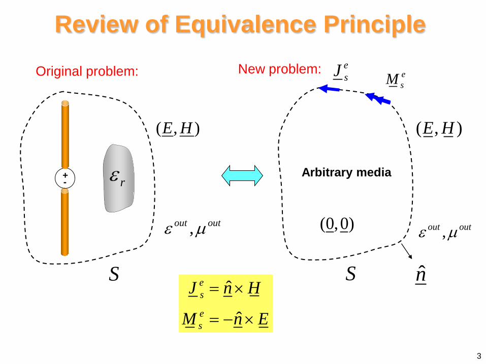
Review of Equivalence Principle New problem:

+ - rε

( , )E H

,out outε µ

Sˆ

ˆ

es

es

J n H

M n E

= ×

= − ×

Original problem:

3

( , )E H

,out outε µ(0,0)

n̂

esJ e

sM

S

Arbitrary media

Review of Equivalence Principle

A common choice (PEC inside):

ˆ

ˆ

es

es

J n H

M n E

= ×

= − ×

( , )E H

,out outε µ

n̂

esJ e

sM

S

PEC

The electric surface current sitting on the PEC object does not radiate, and can be ignored.

4

Model of Patch and Feed

h rεx

AS

Infinite substrate

(aperture)

Patch

Probe

Coax feed

z

5

Model of Patch and Feed

ˆesM z E= − ×Aperture:

h rεx

esM

Magnetic frill model:

h rεx

ASS

( , )E H

Put zero fields Put ground plane

6

Electric Current Model: Infinite Substrate

ˆ ˆ 0ˆ

es tes s

M n E n EJ n H J

= − × = − × =

= × =

Note: The frill is ignored.

The surface S “hugs” the PEC metal.

h rεx

topsJ

probesJ

botsJ

h rεx

SInfinite substrate

( , )E H

Put zero fields Remove patch and probe

7

Let patch top bots s sJ J J= +

Electric Current Model: Infinite Substrate (cont.)

probesJ

patchsJ

Top view

h rεx

patchsJ

probesJ

8

Magnetic Current Model: Infinite Substrate

Put zero fields Remove patch, probe, and frill current Put substrate and ground plane

ˆ 0, ,ˆ 0,

0,

0,

es t bes b

es t

es h

M n E r S SJ n H r S

J r S

J r S

= − × = ∈

= + × = ∈

≈ ∈

≈ ∈

(weak fields)

(approximate PMC)

h rεx

( , )E H

bS

hS

tS

esM

S

9

Exact model:

ˆesM n E= − ×

Approximate model:

Magnetic Current Model: Infinite Substrate (cont.)

h rεx

esJ

esMe

sJesJ

esM

h rεx

esM e

sM

Note: The magnetic currents radiate inside an infinite substrate above a ground plane.

10

Magnetic Current Model: Truncated Substrate

Note: The magnetic currents radiate in free space above a ground plane.

Approximate model:

esM

x

Put zero fields Remove the substrate

rε

x

bS

11

The substrate is truncated at the edge of the patch.

Electric Current Model: Truncated Substrate

rεx

S The patch and probe are replaced by surface currents, as before.

Next, we replace the dielectric with polarization currents.

patchsJ

rε

patch top bots s sJ J J= +

x

12

The substrate is truncated at the edge of the patch.

( )( )

0 0

0 01r

H j Ej E j E

j E j E

ωεω ε ε ωε

ωε ε ωε

∇× =

= − +

= − +

( )0 1polrJ j Eωε ε= −

Electric Current Model: Truncated Substrate (cont.)

0εx

patchsJ

probesJ

polJ

In this model we have three separate electric currents.

13

( ): , ,J patch probe pols s sJ J J J

Comments on Models

Infinite Substrate

The electric current model is exact (if we neglect the frill), but it requires knowledge of the exact patch and probe currents.

The magnetic current model is approximate, but fairly simple.

For a rectangular patch, both models are fairly simple if only the (1,0) mode is assumed.

For a circular patch, the magnetic current model is much simpler (it does not involve Bessel functions).

14

Comments on Models (cont.)

Truncated Substrate

The electric current model is exact (if we neglect the frill), but it requires knowledge of the exact patch and probe currents, as well as the field inside the patch cavity (to get the polarization currents). It is a complicated model.

The magnetic current model is approximate, but very simple. This is the recommended model.

For the magnetic current model the same formulation applies as for the infinite substrate – the substrate is simply taken to be air.

15

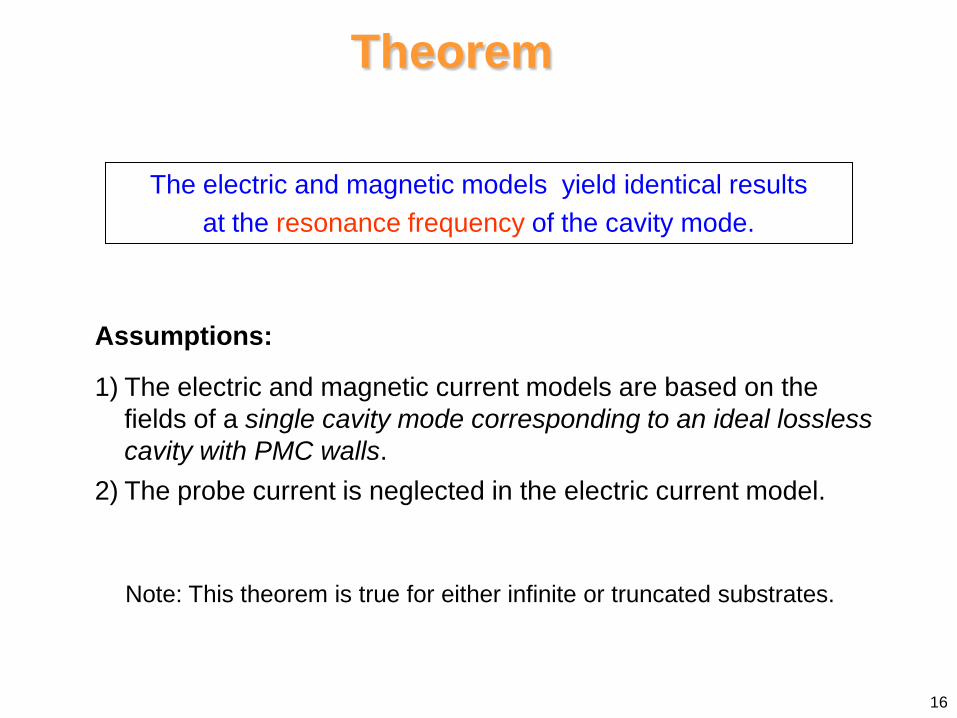
Theorem

Assumptions:

1) The electric and magnetic current models are based on the fields of a single cavity mode corresponding to an ideal lossless cavity with PMC walls.

2) The probe current is neglected in the electric current model.

The electric and magnetic models yield identical results at the resonance frequency of the cavity mode.

16

Note: This theorem is true for either infinite or truncated substrates.

Electric-current model:

ˆesM n E= − ×

Magnetic-current model:

h rεx

esJ

h rεx

esM e

sM

Theorem (cont.)

ˆesJ z H= − ×

(E, H) = fields of resonant cavity mode with PMC side walls

17

Theorem (cont.)

Proof:

( ) ( )0 : , 0,0f f E H= ≠At

Ideal cavity

rεx

PMC

PEC

( , )E H

We start with an ideal cavity having PMC walls on the sides. This cavity will support a valid non-zero set of fields at the resonance frequency f0 of the mode.

18

Proof

Equivalence principle:

Put (0, 0) outside S

Keep (E, H) inside S

xS ( , )E H ( )0,0

PEC

xS PMC ( , )E H

The PEC and PMC walls have been removed in the zero field (outside) region. We keep the substrate and ground plane in the outside region.

Proof for infinite substrate

19

Proof (cont.)

ˆes iJ n H= ×

ˆes iM n E= − ×

Note: The electric current on the ground is neglected (it does not radiate).

Note the inward pointing normal ˆin

20

x( , )E H

esM

esJ

( )0,0 ˆin

Proof (cont.) Exterior Fields:

0e es sE J E M+ + + =

ˆ ˆe patch Jis s sJ n H z H J J= × = − × = =

(The equivalent electric current is the same as the electric current in the electric current model.)

( )

ˆ

ˆˆ

es i

Ms

M n E

n En E

M

= − ×

= + ×

= − − ×

= −

(The equivalent current is the negative of the magnetic current in the magnetic current model.)

21

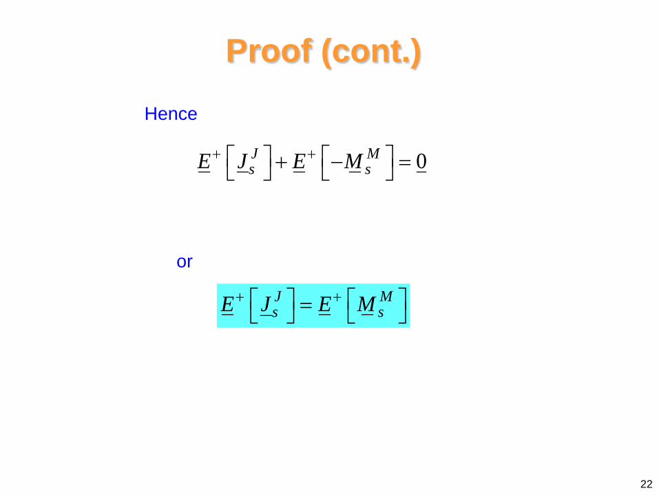
Proof (cont.)

Hence

or

0J Ms sE J E M+ + + − =

J Ms sE J E M+ + =

22

Proof for truncated model

Theorem for Truncated Substrate

xS PMC ( , )E H

PEC

xS PMC ( , )E H

PEC

polJ

Replace the dielectric with polarization current:

23

e patchs s

e Ms s

J J

M M

=

= −

0patch pol MssE J E J E M+ + + + + − =

J MssE J E M+ + =

Proof (cont.)

Hence

x( , )E H e

sM( )0,0

polJ

esJ

patch pol MssE J E J E M+ + + + = or

24

Rectangular Patch

Ideal cavity model:

022 =+∇ zz EkE

( , ) ( ) ( )zE x y X x Y y=

2 0X Y XY k XY′′ ′′+ + =

Let

0z

C

En

∂=

∂

PMC

C

L

W

x

y

Divide by X(x)Y(y):

so

25

2X YkX Y′′ ′′ = − +

2 0X Y kX Y′′ ′′+ + =

Rectangular Patch (cont.) Hence

2( ) constant( ) x

X x kX x′′

= ≡ −

( ) sin cosx xX x A k x B k x= +

( ) cos( )xX x k x=

Choose 1B =

(0) cos( 0) sin( 0) 0x x x x xX k A k k B k k A′ = − = =

( )( ) sin 0x x

x

X L k k LmkLπ

′ = − =

=

General solution:

Boundary condition:

0A =

Boundary condition:

26

so

so

( ) cos m xX xLπ =

2 2 0xYk kY′′

− + + =

( )2 2 2constant x yY k k kY′′= = − − ≡ −

( ) cos n yY yWπ =

( , ) ( , ) cos cosm nz

m x n yE x yL Wπ π =

Returning to the Helmholtz equation,

Following the same procedure as for the X(x) function, we have:

Hence

27

Rectangular Patch (cont.)

where

0222 =+−− kkk yx

22

+

=

Wn

Lmkmn

ππ

µεωmnmnk =

221

+

=

Wn

Lm

mnππ

µεω

2 2

mnr

c m nL Wπ πω

ε = +

Using

we have

Hence

28

Rectangular Patch (cont.)

Current: ˆ ˆpatch

sJ n H z H= × = − ×

( )

( )

1

1 ˆ

1 ˆ ˆ

z

z z

H Ej

z Ej

z E z Ej

ωµ

ωµ

ωµ

−= ∇×

−= ∇×

− = ∇× − ×∇

1zˆH z E

jωμ

so

29

Rectangular Patch (cont.)

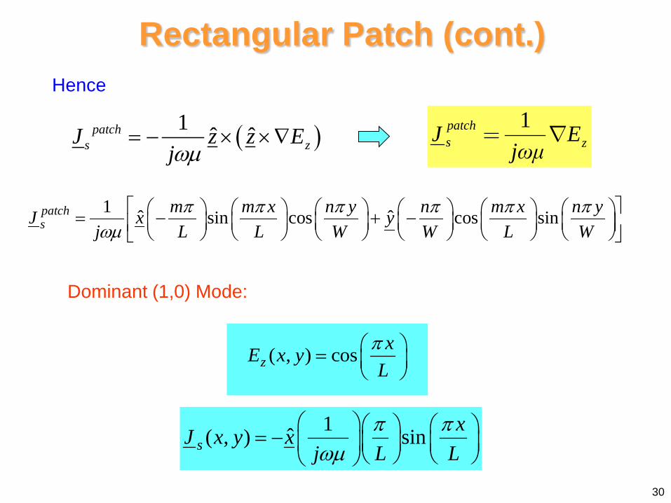
Hence

1patchs zJ E

jωμ

1 ˆ ˆsin cos cos sinpatchs

m m x n y n m x n yJ x yj L L W W L W

π π π π π πωµ

= − + −

Dominant (1,0) Mode:

1ˆ( , ) sinsxJ x y x

j L Lπ π

ωµ = −

( , ) coszxE x y

Lπ =

30

Rectangular Patch (cont.)

( )1 ˆ ˆpatchs zJ z z E

jωµ= − × ×∇

00

( , ) 10

( , ) 0

z

s

E x y

J x yω

==

=

Static (0,0) mode:

This is a “static capacitor” mode.

A patch operating in this mode does not radiate at zero frequency, but it can be made resonant at a higher frequency if the patch is loaded by an inductive probe (a good way to make a miniaturized patch).

31

Rectangular Patch (cont.)

Radiation Model for (1,0) Mode

Electric-current model:

ˆ sinpatchs

xJ xj L Lπ πωµ

= −

L

W

x

y

h rεx

patchsJ

32

Radiation Model for (1,0) Mode (cont.)

Magnetic-current model:

ˆ

ˆ ˆ cos

MsM n E

xn zLπ

= − ×

= − ×

=−==−=

=

0ˆˆ

0ˆˆ

ˆ

yyWyy

xxLxx

nx

y

L

W

33

Hence

ˆ ˆcos

ˆ ˆcos 0 0

ˆ cos

ˆ cos 0

Ms

y y x L

y y xM

xx y WL

xx yL

π

π

π

= − =

− = − ==

− =

=

radiating edges

MsM

L

W

x

y

Radiation Model for (1,0) Mode (cont.)

The non-radiating edges do not contribute to the far-field pattern in the principal planes.

34

Circular Patch

set

a

022 =+∇ zz EkE

( ) cos( )cos

( ) sin( )n

zn

J k n m zEY k n h

ρ

ρ

ρ φ πρ φ

=

( )1/ 22 2

1/ 222

zk k k

mkh

k

ρ

π

= −

= − =

0m =

PMC

35

Circular Patch (cont.) Note: cosφ and sinφ modes are degenerate (same resonance frequency).

( ) ( )cosz nE n J kφ ρ=Choose cosφ :

( ) 0nJ ka′ =( )nJ x′

x

1nx′ 2nx′

0z

a

E

ρρ =

∂=

∂

36

Circular Patch (cont.)

Hence

so

npka x′=

np npr

c xωε

′=

Dominant mode (lowest frequency) is TM11:

11

( , ) (1,1)1.841

n px

=′ =

(1,1)1( , ) cos ( )zE J kρ φ φ ρ=

37

Circular Patch (cont.) Electric current model:

TM11 mode:

1 1 1ˆˆ

1 1ˆˆ cos ( ) ( )sin ( )

J z zs z

n n

E EJ Ej j

k n J k n n J kj

ρ φωµ ωµ ρ ρ φ

ρ φ ρ φ φ ρωµ ρ

∂ ∂= ∇ = + ∂ ∂

′= + −

1 11 1ˆˆ cos ( ) sin ( )J

sJ k J k J kj

ρ φ ρ φ φ ρωµ ρ

′= − −

1, 1n p= =x

y

Very complicated!

38

Magnetic current model:

so

( )ˆˆ ˆ

ˆ

Ms

z

z

M n Ez E

E

ρ

φ

= − ×

= − ×

=

ˆ cos ( )Ms nM n J kaφ φ=

TM11:

1ˆ cos ( )M

sM J kaφ φ=

1, 1n p= =

39

Circular Patch (cont.)

Note:

At

so

1

( ) ( )

cos ( )z a

V h E

h J kaρ

φ φ

φ=

= −

= −

0φ =

0ˆ cosMs

VMh

φ φ = −

0 1(0) ( )V V h J ka≡ = −

Hence 01

ˆ ˆcos ( ) cosMs

VM J kah

φ φ φ φ = = −

40

Circular Patch (cont.)

Ring approximation:

000

cos cosh M M

s sVK M dz h M h Vhφ φ φ φ φ = = = − = −

∫

0( ) cosK Vφ φ φ= −

x

y

( )K φ

h rεx

esM

h rεx

K

ˆK Kφφ=

41

Circular Patch (cont.)