SAR Day 2 Lecture 4 Introduction to Modelling C. Schmullius 1
Prof. Dr. Christiana SchmulliusDr. Leif Eriksson, Dipl.-Geogr. Tanja Riedel
Dr. Maurizio Santoro, Dr. Christian Thiel
Department for Geoinformatics and Remote SensingFriedrich-Schiller-University Jena, Germany
SAR Day 2 Lecture 4 Introduction to Modelling C. Schmullius 2
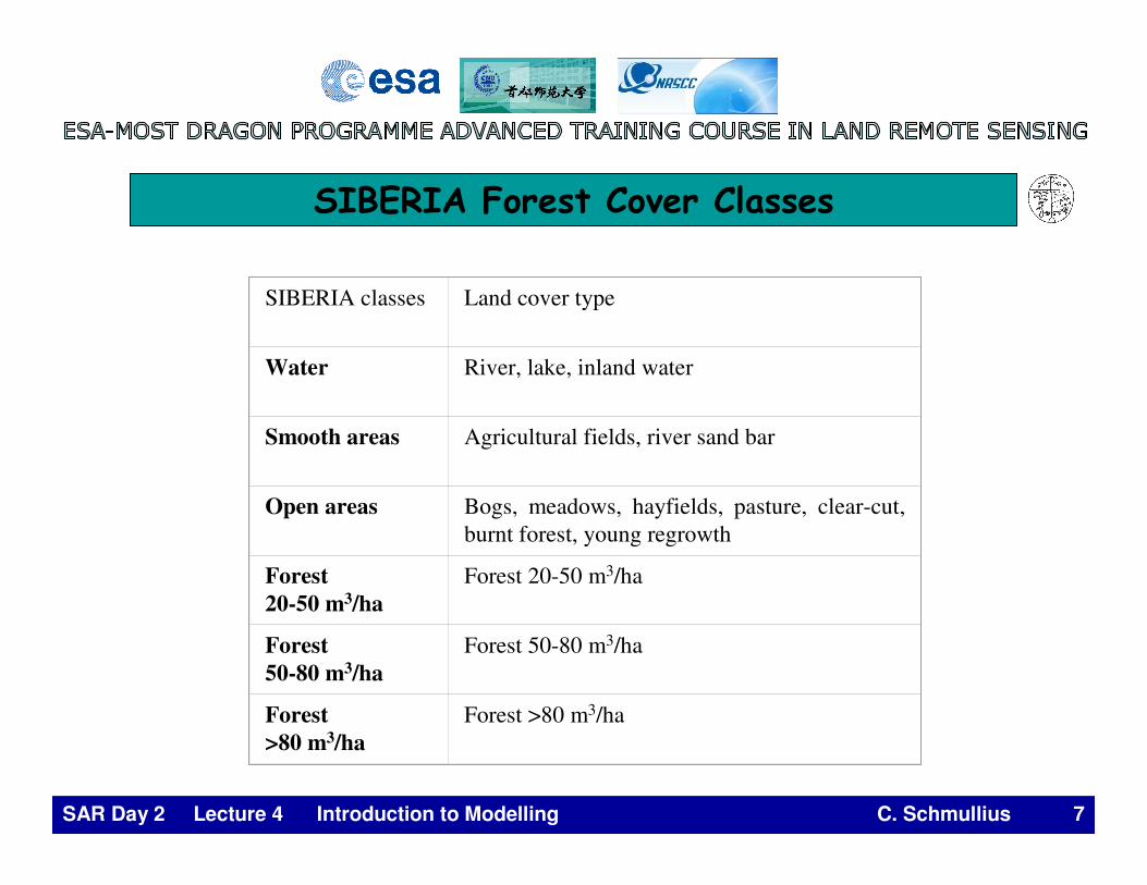
����������� ���������� ���� �����
ERS coherence image
JERS intensity image
Use model to calculate
class means
Maximum LikelihoodClassifier
Iterated ContextualProbability Classifier
(ICP)
SAR Day 2 Lecture 4 Introduction to Modelling C. Schmullius 3
�������������������� ������ �• Histograms vary from scene to scene.
– How to capture variance? From the scenes themselves.
Simulated Histograms of Stem Volume Classes and Overall Class „Forest“.
Characteristic Values
Wagner et al., RSE, 2003
SAR Day 2 Lecture 4 Introduction to Modelling C. Schmullius 4
�������������� ����������
• Ground truth data determine model for ERS coherence and JERS-1 intensity
Coherence Model:γ75 .. CharacteristicCoherence Percentile
( ) 1227575 58.033.0)(
v
ev−
⋅⋅++= γγγ
Test data to determine coherency model.
Wagner et al., RSE, 2003
SAR Day 2 Lecture 4 Introduction to Modelling C. Schmullius 5
��� ����������������������( ) ( ) γγγγγ V
v
ev−
∞∞ ⋅−+= 0
750 γγ γγ ⋅+= ba
( ) γγγγ γγVv
ebav−
⋅−++= 7575 )1()(
( ) 1.1227575 581.0330.0)(
v
ev−
⋅⋅++= γγγ
75γγ ≈∞
v = growing stock volume
γ0 = coherence at v = 0 m3/ha (non-forest)
γ∞ = coherence for asymptotic values of v(corresponding to dense forest)
γ75 = value where the coherence distribution reach 75% of the maximum value (see fig.)
Vγ = characteristic v value where the exponential function has decreased by e-1
Wagner et al., RSE, 2003
SAR Day 2 Lecture 4 Introduction to Modelling C. Schmullius 6
( ) σσσσσ Vv
ev−
∞∞ ⋅−+= 00 )(
34.10775
0 46.2)(v
ev−
⋅−= σσ
Wagner et al., RSE, 2003
��� ����������������������
SAR Day 2 Lecture 4 Introduction to Modelling C. Schmullius 7
� ������ ������������ �����
SIBERIA classes Land cover type
Water River, lake, inland water
Smooth areas Agricultural fields, river sand bar
Open areas Bogs, meadows, hayfields, pasture, clear-cut, burnt forest, young regrowth
Forest 20-50 m3/ha
Forest 20-50 m3/ha
Forest 50-80 m3/ha
Forest 50-80 m3/ha
Forest>80 m3/ha
Forest >80 m3/ha
SAR Day 2 Lecture 4 Introduction to Modelling C. Schmullius 8
����������� ��
Radar Image Mosaic
111 Radar Image Maps
Forest Cover Mosaic
96 Forest Cover Maps
SAR Day 2 Lecture 4 Introduction to Modelling C. Schmullius 9
Pang Yong, Annual Progress Report 2004, CAF
� �� ���������� ������ �������������� �����������������
SAR Day 2 Lecture 4 Introduction to Modelling C. Schmullius 10
The retrieval process can be divided in four parts: 1. Model selection2. Model training3. Retrieval4. Accuracy assessment
Growing stock volume = stem volume [m3/ha]
Leif Eriksson et al., ForestSAT 2005
Stem volume retrieval – Methodology 1
SAR Day 2 Lecture 4 Introduction to Modelling C. Schmullius 11
Regression model
�: coherence
V: growing stock volume
Regression parameters
A: dynamic range
B: slope
C: offset
( ) CeAV VB +∗= ∗γ
Leif Eriksson et al., ForestSAT 2005
Stem volume retrieval – Methodology 2
SAR Day 2 Lecture 4 Introduction to Modelling C. Schmullius 12
Best results for JERS-1:RMSE = 60 m³/haRelative RMSE = 43 %R² = 0.75
Best results for ERS-1/2:RMSE = 57 m³/haRelative RMSE = 37 %R² = 0.73
Leif Eriksson et al., ForestSAT 2005
Stem volume retrieval – Results
SAR Day 2 Lecture 4 Introduction to Modelling C. Schmullius 13
Regression model
JERS-1 coherence
JERS-1 backscatter
SIBERIA algorithm
JERS-1 coherence
JERS-1 backscatter
SIBERIA algorithm
ERS-1/2 coherence
JERS-1 backscatter
Forest inventory
Leif Eriksson et al., ForestSAT 2005
Interferometric Water Cloud Model
SAR Day 2 Lecture 4 Introduction to Modelling C. Schmullius 14
( )Voveg
Vogr
ofor ee ββ σσσ −− −+= 1
����������������� � ��������� ��������������������� ��������
� �����������
����������������� �������������� � �������������
( ) ( )1
1−−−−− −+= αωββ
σσ
γσσ
γγ hjofor
oveg
vegVV
ofor
ogr
grfor eee
������������� ��� � ��������� ��������������������� ��������
�������������� � ���������������������������������������
� �������� ���� ������������� ���
Interferometric Water Cloud Model
Santoro et al., RSE, 2002
SAR Day 2 Lecture 4 Introduction to Modelling C. Schmullius 15
������������ ������� � �� ������
�����������!��������σ "���#�σ "� #�β, γ�������γ� ������(γ, �$������ ���
!%& '!%&
�������� ������!��������σ 0���#�σ "� ����β ������(σ ο, �$������ ���
Santoro et al., RSE, 2002
SAR Day 2 Lecture 4 Introduction to Modelling C. Schmullius 16
������������
(��� ������������������������� ���� � ���� ����������������������������������
��!%&�������� ����������) �������������� ������
*�!%&�+������, ��� ����) ����������� ������
-� ����)���� ��
�$������ ����������#��$������� ������
��� '!%&�������� �) ������� ���� ������ �������
� . �/��� �0������������
� 1���� /� �0������������� ������� �������
2"�3
*"�3
�4�3
54�3
Error
Local survey
Santoro et al., RSE, 2002
SAR Day 2 Lecture 4 Introduction to Modelling C. Schmullius 17
*���������/���)� ������������
!%&�+������, ��� ���
%�&!���"��* ��
%��������%�&!��6�3
'!%&��������
%�&!��**��* ��#�
%��������%�&!�����3
Santoro et al., RSE, 2002
SAR Day 2 Lecture 4 Introduction to Modelling C. Schmullius 18
��Model-based retrieval procedure is robust and consistent�Multi-temporal combination to be preferred�C-band „tandem“ coherence: ideal�L-band backscatter: reliable
�Accuracy comparable to ground-based surveys
��Importance of reference ground-truth and SAR data�C-band „tandem“ coherence: depends on weather conditions�L-band backscatter: few images at ideal conditions
Santoro et al., RSE, 2002
Conclusions – Stem volume retrieval