31
Prof. Ji Chen Notes 12 Transmission Lines (Smith Chart) ECE 3317 1 Spring 2014
| Date post: | 15-Dec-2015 |
| Category: |
Documents |
| Upload: | kurtis-dewhirst |
| View: | 221 times |
| Download: | 1 times |

1
Prof. Ji Chen
Notes 12 Transmission Lines
(Smith Chart)
ECE 3317
Spring 2014

2
Smith Chart
The Smith chart is a very convenient graphical tool for analyzing transmission lines and studying their behavior.
A network analyzer (Agilent N5245A PNA-X) showing a Smith chart.

3
Smith Chart (cont.)
Phillip Hagar Smith (April 29, 1905–August 29, 1987) was an electrical engineer, who became famous for his invention of the Smith chart.Smith graduated from Tufts College in 1928. While working for RCA, he invented his eponymous Smith chart. He retired from Bell Labs in 1970.
Phillip Smith invented the Smith Chart in 1939 while he was working for The Bell Telephone Laboratories. When asked why he invented this chart, Smith explained: “From the time I could operate a slide rule, I've been interested in graphical representations of mathematical relationships.”
In 1969 he published the book Electronic Applications of the Smith Chart in Waveguide, Circuit, and Component Analysis, a comprehensive work on the subject.
From Wikipedia:

4
Smith Chart (cont.)
1
1Nin
zZ z
z
The Smith chart is really a complex plane:
Re z
Im z
1
2
2
j zL
j lL
z e
e
L z2 l
0
0
ZΓ
ZL
LL
Z
Z
z l

5
Smith Chart (cont.)
1
1N Nin in
zR jX
z
Denote z x jy (complex variable)
1
1N Nin in
x jyR jX
x jy
1 1N Nin inx jy R jX x jy
1 1
1
N Nin in
N Nin in
x R yX x
x X yR y
Real part:
Imaginary part:
so

6
1 1
1
N Nin in
N Nin in
x R yX x
x X yR y
Smith Chart (cont.)
From the second one we have
11
N Nin in
yX R
x
Substituting into the first one, and multiplying by (1-x), we have
1 1 11
N Nin in
yx R y R x
x
2 21 1 1 1N Nin inx R y R x x

7
Smith Chart (cont.)
2 21 1 1 1N Nin inx R y R x x
2 2 21 1 1N Nin inx R y R x
2 21 2 1 1 0N N N Nin in in inx R xR R y R
2 21 2 1 1N N N Nin in in inx R xR y R R
2 2 12
1 1
N Nin in
N Nin in
R Rx x y
R R
Algebraic simplification:

8
Smith Chart (cont.)
2 2 12
1 1
N Nin in
N Nin in
R Rx x y
R R
2 2
2 1
1 1 1
N N Nin in in
N N Nin in in
R R Rx y
R R R
22
22
1 1
1 1
N N NNin in inin
N Nin in
R R RRx y
R R
2
22
1
1 1
Nin
N Nin in
Rx y
R R

9
Smith Chart (cont.)
2
22
1
1 1
Nin
N Nin in
Rx y
R R
This defines the equation of a circle:
, ,01
Nin
c c Nin
Rx y
R
center: radius:1
1 Nin
RR
Re z
Im z
0NinR
1NinR
3NinR
0.2NinR
NinR
1cx R Note:

10
Smith Chart (cont.)
1 1
1
N Nin in
N Nin in
x R yX x
x X yR y
Now we eliminate the resistance from the two equations.
From the second one we have:
1 NinN
in
x X yR
y
Substituting into the first one, we have
11 1
Nin N
in
x X yx yX x
y

11
Smith Chart (cont.)
Algebraic simplification:
11 1
Nin N
in
x X yx yX x
y
2 21 1 1 0N Nin inx X y x y X y x
2 21 2 0N Nin inx X y y X
2 221 0
Nin
x y yX

12
Smith Chart (cont.)
2 221 0
Nin
x y yX
2 2
2 1 11
N Nin in
x yX X
This defines the equation of a circle:
1, 1,c c N
in
x yX
center: radius:1
Nin
RX
cy RNote:

13
Smith Chart (cont.)
This defines the equation of a circle: 1, 1,c c N
in
x yX
1Nin
RX
Re z
Im z1N
inX
1NinX
0NinX
NinX
3NinX
3NinX
0.5NinX
0.5NinX

14
Smith Chart (cont.)
Re z
Im z
z
Actual Smith chart:

15
Smith Chart (cont.)
Important points:
S/C O/CPerfect Match
1circle
jX
= 0
( 1)
NinR
z
( 0)z
1
1
NinNin
Z zz
Z z

16
Smith Chart (cont.)
( )Lz Movement in negative direction Clockwise motion on
t
circle of co
oward genera
nstan
tor
t
2 2
2 2
1 1 1( )
1 1 1
j z j lN L Lin j z j l
L L
z e eZ z
z e e
ΓL
Im z
Re z
L
z
angle change = 2l
Transmission LineGeneratorLoad
z = -l
To generator
Zg
z
ZL
z = 0
Z0
S

17
Smith Chart (cont.)
2
2
1
1
j zN Lin j z
L
eZ z
e
We go completely around the Smith chart when
/ 2l
22 2 2 2
2z l
ΓL
Re z
Im z

18
Smith Chart (cont.)
2
22
4
4
z
z
z
l
In general, the angle change on the Smith chart as we go towards the generator is:
2 2j z j j z jL L Lz e e e e
4l
ΓL
Re z
Im z
The angle change is twice the electrical length change on the line: = -2( l).

19
Smith Chart (cont.)
Note:
The Smith chart already has wavelength scales on the perimeter for your convenience (so you don’t need to measure angles).
The “wavelengths towards generator” scale is measured clockwise, starting (arbitrarily) here.
The “wavelengths towards load” scale is measured counterclockwise, starting (arbitrarily) here.

Reciprocal Property
2
2
1
1
j zN Lin j z
L
eZ z
e
Go half-way around the Smith chart:
/ 4l
22 2
4z
ΓL
Re z
Im z
1( )
( )Nin N
in
Z BZ A
10
1N Lin
L
Z
1
1N Lin
L
Z l
B
A
0
0
0
1 1
/
1/
1/
Nin in
in
in
Nin
Z z Z z Z
Z z
Z
Y z
Y
Y z
20
Normalized impedances become normalized admittances.

21
Normalized Voltage
max max
min min
V 1
V 1-
L
L
z
V z
V
+ 2V( ) = V 1+Γ 1+Γj zLz z e z
Normalized voltage
We can use the Smith chart as a crank diagram.
maxVminV
V( )z
ΓL
Γ z
+V 1z Assume

22
SWR
ΓL
2Γ Γ j zLz e Γ z
The SWR is read off from the normalized resistance value on the positive real axis.
As we move along the transmission line, we stay on a circle of constant radius.
0
Ninin
RSWR R
Z
0N Nin inZ R Z real
On the positive real axis:
(from the previous property proved about a real load)
Positive real axis

23
Example
=0.707 45L
maxVminVΓL
V z 45ZN
L
X
Given:
1Z 1 2
1N LL
L
j
45 / 4 rad
Use the Smith chart to plot the magnitude of the normalized voltage, find the SWR, and find the normalized load admittance.
1.707
0.293
load
5
16
V(z)
16
z
=0.707 L
V (z) 1
22 2 =
4l l
16l
1 =1.707 L
Set

24
Example (cont.)
SWR = 5.8
/ 16 0.1875
0.2 0.4 NLY j
=0.707 45
1 2
L
NLZ j
45
1NinR
2NinX

25
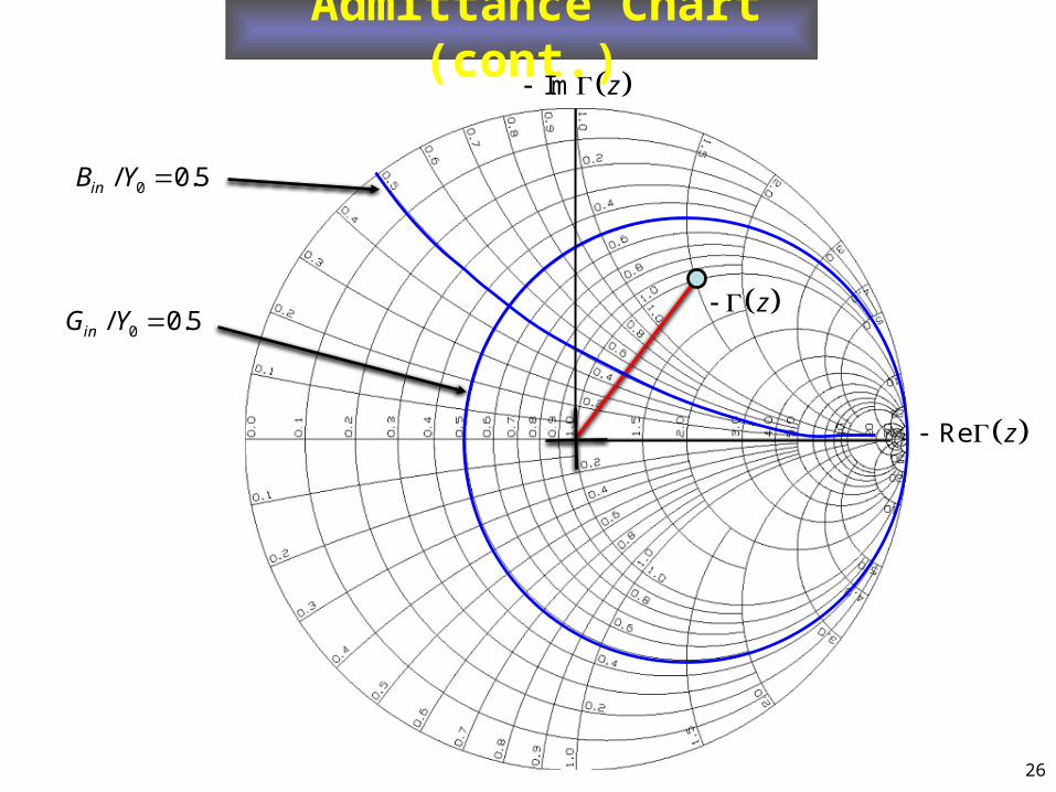
Smith Chart as an Admittance Chart
The Smith chart can also be used as an admittance calculator instead of an impedance calculator.
1
1Nin
zZ z
z
0 0 0
1/ 1 1
1/ /in inN
in Nin in
Y z Z zY z
Y Z Z z Z Z z
1
1N
in
zY z
z
1
1N
in
zY z
z
where z z
Hence
or
26
Admittance Chart (cont.)
Re z
Im z
z
0/ 0.5inB Y
0/ 0.5inG Y

27
Comparison of Charts
Impedance chart
Inductive region
0NinX
Capacitive region
0NinX
Im z

28
Comparison of Charts (cont.)
Admittance chart
Capacitive region
0NinB
Inductive region
0NinB
Im z

29
Using the Smith chart for Impedance and Admittance Calculations
We can convert from normalized impedance to normalized admittance, using the reciprocal property (go half-way around the smith chart).
We can then continue to use the Smith chart on an admittance basis.
We can use the same Smith chart for both impedance and admittance calculations.
The Smith chart is then either the plane or the - plane, depending on which type of calculation we are doing.
For example:
30
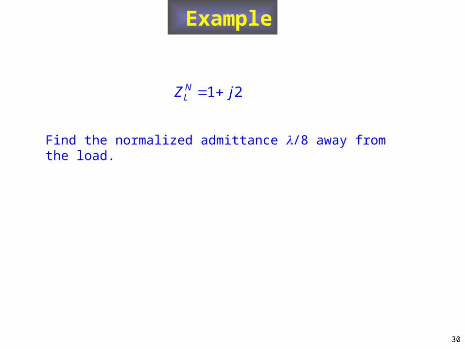
Example
1 2 NLZ j
Find the normalized admittance l/8 away from the load.

Admittance Chart (cont.)
31
0.2 . 0 4NLY j
1 2 NLZ j
0.23 . 0 48NinY j
o90
2 4
14
8
2
ll
0.23 0.48 NinY j
Answer:
Re Rez z or
Im Imz z or
o90


![Prof. David R. Jackson Notes 15 Plane Waves ECE 3317 [Chapter 3]](https://static.documents.pub/doc/80x56/56649f225503460f94c3b238/prof-david-r-jackson-notes-15-plane-waves-ece-3317-chapter-3.jpg)


