Professor Charles Perringsperrings.faculty.asu.edu/pdf_papers_Perrings/Perrings_IJEES_(2006).pdfAlaa...

Special Issue in Honor of

Professor Charles Perrings

Volume 6 Number F06 Fall 2006

ISSN 0973-1385

International Journal of Ecological Economics & Statistics (IJEES)

ISSN 0973-1385

Editorial Board

Editor-in-Chief:

Kaushal K. Srivastava

Director,Centre for Environment, Social & Economic Research (CESER)Post Box 113, Roorkee-247667, INDIA email: [email protected], [email protected]

Editors:

Peter Soderbaum, Mälardalen University , Sweden

Wang Songpei, Chinese Academy of Social Sciences , China

Roberto Roson, University Cà Foscari of Venice, Italy

Barry Solomon, Michigan Technological University , USA

Sergio Ramiro Peña-Neira, Universidad del Mar , Chile

Tanuja Srivastava, Indian Institute of Technology, Roorkee, India

Timothy Randhir, University of Massachusetts, USA

Bernd Siebenhüner, Oldenburg University , Germany

Jyoti K. Parikh, Integ. Research & Action for Development , India

Miriam Kennet, Green Econmics Institute , UK

Michael Ahlheim, University of Hohenheim, Germany

Associate Editors:

Klaus Hubacek, University of Leeds, UK

R. B. Dellink, Wageningen University, Netherlands

Stanislav Shmelev, Open University, UK

Paul C. Sutton, University of Denver, USA

Unai Pascual, University of Cambridge, UK

Continued----

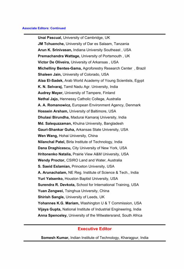
Associate Editors: Continued

Unai Pascual, University of Cambridge, UK

JM Tchuenche, University of Dar es Salaam, Tanzania

Arun K. Srinivasan, Indiana University Southeast , USA

Premachandra Wattage, University of Portsmouth , UK

Victor De Oliveira, University of Arkansas , USA

Michelliny Bentes-Gama, Agroforestry Research Center , Brazil

Shaleen Jain, University of Colorado, USA

Alaa El-Sadek, Arab World Academy of Young Scientists, Egypt

K. N. Selvaraj, Tamil Nadu Agr. University, India

Audrey Mayer, University of Tampere, Finland

Nethal Jajo, Hennessy Catholic College, Australia

A. A. Romanowicz, European Environment Agency, Denmark

Hossein Arsham, University of Baltimore, USA

Dhulasi Birundha, Madurai Kamaraj University, India

Md. Salequzzaman, Khulna University, Bangladesh

Gauri-Shankar Guha, Arkansas State University, USA

Wen Wang, Hohai University, China

Nilanchal Patel, Birla Institute of Technology, India

Dana Draghicescu, City University of New York, USA

Hritonenko Natalia, Prairie View A&M University, USA

Wendy Proctor, CSIRO Land and Water, Australia

S. Saeid Eslamian, Princeton University, USA

A. Arunachalam, NE Reg. Institute of Science & Tech., India

Yuri Yatsenko, Houston Baptist University, USA

Surendra R. Devkota, School for International Training, USA

Yuan Zengwei, Tsinghua University, China

Shirish Sangle, University of Leeds, UK

Yohannes K.G. Mariam, Washington U & T Commission, USA

Vijaya Gupta, National Institute of Industrial Engineering, India

Anna Spenceley, University of the Witwatersrand, South Africa

Executive Editor

Somesh Kumar, Indian Institute of Technology, Kharagpur, India

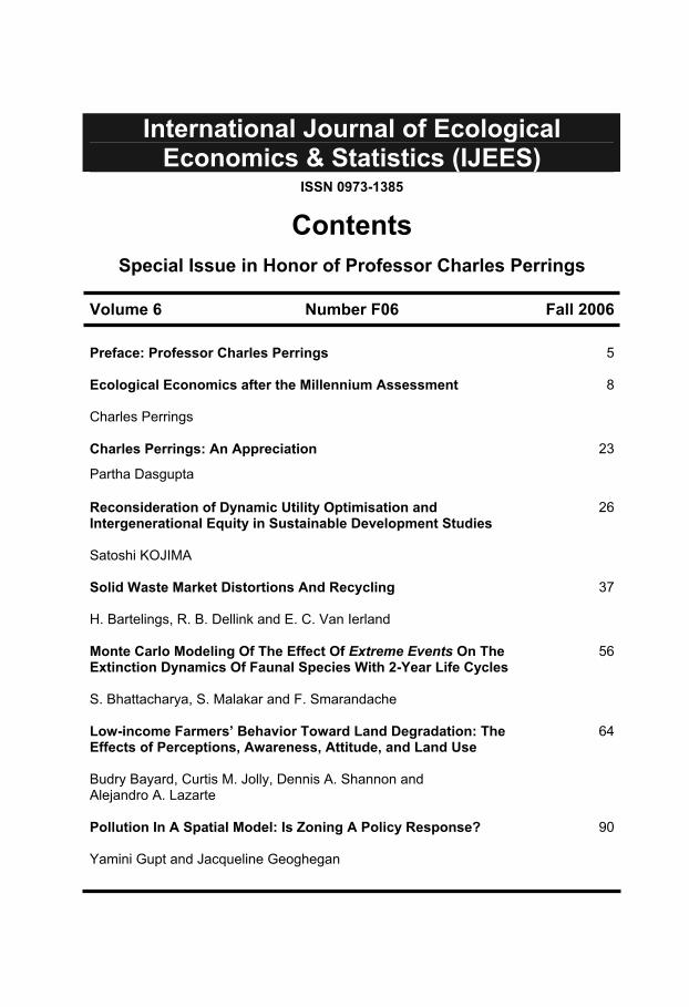
International Journal of Ecological Economics & Statistics (IJEES)

ISSN 0973-1385

Contents

Special Issue in Honor of Professor Charles Perrings

Volume 6 Number F06 Fall 2006

Preface: Professor Charles Perrings 5

Ecological Economics after the Millennium Assessment

Charles Perrings

8

Charles Perrings: An Appreciation

Partha Dasgupta

23

Reconsideration of Dynamic Utility Optimisation and Intergenerational Equity in Sustainable Development Studies

Satoshi KOJIMA

26

Solid Waste Market Distortions And Recycling

H. Bartelings, R. B. Dellink and E. C. Van Ierland

37

Monte Carlo Modeling Of The Effect Of Extreme Events On The Extinction Dynamics Of Faunal Species With 2-Year Life Cycles

S. Bhattacharya, S. Malakar and F. Smarandache

56

Low-income Farmers’ Behavior Toward Land Degradation: The Effects of Perceptions, Awareness, Attitude, and Land Use

Budry Bayard, Curtis M. Jolly, Dennis A. Shannon and Alejandro A. Lazarte

64

Pollution In A Spatial Model: Is Zoning A Policy Response?

Yamini Gupt and Jacqueline Geoghegan

90

Preface: Professor Charles Perrings

Dr. Charles Perrings is a Professor of Environmental Economics at the Global

Institute for Sustainability at Arizona State University since August 2005. Professor

Perrings is a world renowned ecological economist who has made an extensive

contribution to our understanding of the economics of biodiversity. His applied

research extends to a variety of areas that include biodiversity, water resources, and

resilience of coupled ecological-economic systems. Also, he has conducted research

on the problem of sustainable development for decades, much of which has

concerned Central and Southern Africa.

His earlier academic positions have been as Professor of Environmental Economics

and Environmental Management at the University of York; Professor of Economics at

the University of California, Riverside; Director of the Biodiversity Program of the

Beijer Institute, Stockholm; Professor of Economics at the University of Botswana;

and Associate Professor of Economics at the University of Auckland. He has been

editor of the Cambridge University Press journal, Environment and Development

Economics and several other journals in environmental, resource and ecological

economics, and in conservation ecology. He is a Past President of the International

Society for Ecological Economics and is currently the Vice-President of the Scientific

Committee of Diversitas, an international program of biodiversity science. Professor

Perrings is an advisor to various governmental, intergovernmental and international

non-governmental organizations as well as research funding agencies.

Prof. Perrings has published extensively in leading journals in the area that include

Journal of Marine Science, Ecological Modeling, Trends in Ecology and Evolution,

Ecological Economics, Journal of Environmental Management, Conservation

Biology, Philosophical Transactions of the Royal Society of London, Scottish Journal

of Political Economy, American Journal of Agricultural Economics, Environment and

Resource Economics, Bulletin of Marine Science, American Journal of Physical

Anthropology, Journal of Environmental Economics and Management, and

Conservation Ecology.

Professor Perrings’ applied research is centred on three main issues: biodiversity,

water and the resilience of coupled ecological-economic systems. The work on bio-

International Journal of Ecological Economics & Statistics (IJEES)Fall 2006, Vol. 6, No. F06; Int. J. Ecol. Econ. Stat.ISSN 0973-1385; Copyright © 2006 IJEES, CESER

diversity relates to identifying the causes of biodiversity change in different ecological

and economic systems. These include climatic changes, sea level rise, social

factors, market failures associated with the lack of well-defined rights to biological

resources. Systems that are being studied in this way include agro-ecosystems

(arable and livestock), lakes and semi-arid rangelands. His work also looks at the

consequences of biodiversity change in terms of the stock of genetic information, the

impact on the flow of economically valuable goods and services, and the capacity of

the system to withstand stresses and shocks. This contributes to a greater

understanding of the link between stability, resilience and the sustainability of

ecological-economic systems.

Professor Perrings’ has also contributed to the development of decision-models for

dealing with problems that are characterised by sensitivity to initial conditions, path

dependence, abrupt if not discontinuous change at threshold values of selected

biological resources, fundamental uncertainty and irreversibility. His current work

includes models of the decision-problem in the case of invasive pests and pathogens

where conventional risk assessment fails due to the fundamental uncertainty of novel

events, and the potential irreversibility of the costs of successful invasion. Professor

Perrings has been involved in the development of strategies, policies and

instruments to address the problem of biodiversity loss at multiple spatial and

temporal scales. His collaborative work has led to a re-evaluation of the significance

of the local versus the global public good dimensions of biodiversity conservation.

Professor Perrings’ work on water involves the development of wetland models. He

studies the correlations between economic uses of wetland resources and wetland

functions, and the state of the wetlands. The study has focussed on wetlands in

Argentina (Ibera) and East Africa (Lake Victoria). The main feature of the work is that

it involves spatially explicit models. He further deals with growth functions of stocks

in fisheries models that are not spatially explicit. It captures the effect of economic

activities on the parameters or structure of the model. Two specific applications,

freshwater fisheries in Lake Malawi and Penaeid shrimp fisheries in the Gulf of Paria,

Trinidad, exhibit that the approach can capture quite complex environmental effects

with fairly minimal data requirements. The Malawi study has explored the problem of

changes in the diversity of the fish catch through a bio-economic diversity index (a

Simpson’s index weighted by the market price of fish). Not only does it substantially

6 International Journal of Ecological Economics & Statistics

improve the fit of the fisheries model, but it turns out to offer some very interesting

implications for the effect of different regulatory and property rights regimes on fish

biodiversity.

Professor Perrings and his co-workers were the first to identify the relevance of the

ecological notion of resilience to the problem of sustainability. They identify an

ecological economic system as a stochastic process that will flip from one state

(stability domain) to another. This supposes that the system can converge on any

one of a number of possible states, depending on initial conditions. For a given set of

initial conditions, a given disturbance regime, and a given state of nature, it may be

possible to estimate the probability that the system will converge in some finite time

to some other state of nature. The connection with sustainability is direct. If the

transition probabilities are known, it is possible to estimate either the time the system

occupies a particular state (the sustainability of that state), or the time to converge to

any other state (the time to sustainability). One may also estimate the robustness of

the system under a particular disturbance regime to change in any particular

direction.

The work suggests that we can analyse the evolution of an ecological-economic

system under different initial conditions. This makes it possible to compare the long-

run implications of different initial conditions in terms of the sustainability or resilience

of the system under each. Some progress has been made in developing methods to

estimate empirically the loss of resilience in managed ecosystems.

The work of Professor Charles Perrings has far reaching implications for economic-

ecological balance, sustainable development and resilience of economies specially

those in the developing countries. We dedicate this volume to his great contributions.

IJEES appreciatively acknowledge, for valuable information about Professor Perrings

and his contributions, the following resources:

http://cdsagenda5.ictp.trieste.it/askArchive.php?base=agenda&categ=a0258&id=a0258s23t5/recording

http://www.ens-newswire.com/ens/jul2006/2006-07-19-01.asp, http://www.public.asu.edu/~cperring/,http://www.sustainable.org.nz/conference2003/plenaryspeakers.htm, http://ec.europa.eu/research/rtdinfo/45/article_2497_en.html,http://www.feem.it/Feem/Pub/Publications/WPapers/WP2003-111.htm, http://www.bio-era.net/be_company_board.php

Int. J. Ecol. Econ. Stat.; Vol. 6, No. F06, Fall 2006 7

Ecological Economics after the Millennium Assessment

Charles Perrings

Global Institute of Sustainability Arizona State University

Box 873211, Tempe, AZ 85287-3211, USA e-mail: [email protected]

Abstract

The Millennium Ecosystem Assessment has changed the way that we think about the interaction between social and ecological systems. By connecting ecological functioning, ecosystem processes, ecosystem services and the production of marketed goods and services it has identified ecological change as an economic problem. It has also drawn attention to a new dimension of the environmental sustainability of economic development. The Hartwick rule for the reinvestment of Hotelling rents on exhaustible and renewable natural resources provides one basis for evaluating the sustainability of extraction policies. The MA’s focus on the regulating services provides another. The regulating services offered by ecosystems limit the variability of ecosystem functioning, processes and the production of marketed goods and services. They help to conserve the resilience and hence sustainability of ecosystems. This offers both a challenge and an opportunity to ecological economists. The challenge is to understand the linkages between such services and the capacity of economic systems to function over a range of environmental conditions. The opportunity stems from the fact that the field is uniquely placed to meet this challenge.

Mathematics Subject Classification 2000: 91B76, 91B02 JEL Classification: N50, Q50, Q57

Introduction

A number of studies of the evolution of ecological economics have identified several

common features of work in the field. These include the perception that the economy is

embedded in and constrained by the environment; that the economy and its environment co-

evolve through time, and that the coupled system is complex and adaptive, exhibiting path

dependence, non-linearity, and sensitivity to initial conditions; that this generates

fundamental uncertainty about the future consequences of current actions; and that for any

given set of technologies there is a sustainable scale of the economy. Röpke (2005a, 2005b)

has also, however, drawn attention to the fact that the field has developed in many different

directions. This is partly as a function of the disciplinary background of the people involved,

and partly a function of the institutional, cultural and environmental conditions in which they

International Journal of Ecological Economics & Statistics (IJEES)Fall 2006, Vol. 6, No. F06; Int. J. Ecol. Econ. Stat.; 8-22ISSN 0973-1385; Copyright © 2006 IJEES, CESER

themselves operate. The International Society for Ecological Economics is an organization

with a widely distributed membership, organized in a number of regional societies. The

research foci of members of the regional organizations in India, Africa and Latin America

tend to be very different from those in the USA, Canada, Europe or Australia/New Zealand.

In thinking about where the field is likely to go in the future, I want to focus on a single area

– albeit a very important one. This is not the only direction that the field will go. Indeed, the

only thing I am sure about is that ecological economics will continue to push the frontiers of

knowledge on wider front than most fields of equivalent size, simply because of its

transdisciplinarity and the heterogeneous nature of its practitioners. But it is an area where

the stakes are extraordinarily high for all of us. It is the impact of environmental change on

regulating ecosystem services, and the consequences this has for human well-being.

Ecological Economics has published (or has in press) a little over a hundred papers on

ecosystem services. A number of notes were generated through the policy forum conducted

around Costanza et al (1997), and extended papers appeared in special issues of the journal in

1999 and 2002. However, there has been an explosion of interest in the topic since the results

of the MA started to appear. One fifth of all of the papers published in the journal on

ecosystem services have either appeared or are due to appear in 2006. This is a major growth

area within the field.

Why is it important? Ecosystem services include not just the provision of foods, fuels and

fibres and well-understood beneficial phenomena such as pollination, watershed protection,

habitat provision and so on, but also the mechanisms that regulate the impact of stresses and

shocks (Dirzo and Raven, 2003). Amongst these, for example, is disease regulation. The

establishment and spread of introduced pests and pathogens, including emergent zoonotic

diseases like the ebola virus, HIV, SARS or avian flu, may turn out to have more impact on

human wellbeing over timescales that matter than many other environmental threats currently

attracting attention (Daszak and Cunningham, 1999, 2000). The severity of the impact of

these diseases, however, depends on environmental conditions (e.g. UNAIDS, 2006). The

regulating ecosystem services determine the capacity of ecosystems both to regulate the

impact of these shocks, and to respond to changes in environmental conditions without losing

functionality (Kinzig et al, 2006). This is a dimension of the environmental sustainability that

has been largely ignored by economists. It turns out that the regulating services are important

wherever there is a distribution of outcomes, and wherever decision-makers care about the

properties of that distribution. Both variance and kurtosis matter to risk-averse decision-


makers. Like the institutions of market economies, the regulating services of ecosystems

affect the distribution of outcomes through both the capacity to respond to perturbations and

the severity of those perturbations. It is hard to imagine a more critical set of issues than those

surrounding the decline in regulating ecosystem services.

The Millennium Assessment

The Millennium Assessment has fundamentally changed the landscape in ecosystem service

research. By switching attention from the underlying ecological processes and functioning to

the services that confer benefits or impose costs on people it has brought the analysis of

ecosystem services into the domain of economics – and in so doing has created a natural

niche for those working in the field of ecological economics. Although ecological economics

is much more than the union of ecology and economics, it was the perception that social and

ecological processes are integrally linked that originally spawned the field. Many ecological

economists are still concerned to understand: (a) how economic activity, ecological

functioning and ecological processes are related, (b) what that means for the value of

environmental assets where the latter are either public goods/bads or are not subject to well-

defined property rights, and (c) what options are available to deal with the resulting

challenges to both efficiency and equity. For such people the research agenda created by the

MA is an especially attractive one.

So what did the MA do that opens the door to ecological economics? It defined ecosystem

services in terms of the benefits yielded by ecosystems (as composite assets), distinguishing

between four broad categories of benefit: provisioning services, regulating services, cultural

services and supporting services. Of the four categories, the first is most familiar.

Provisioning services cover the renewable resources that had been the focus of much work in

environmental and resource economics in the last three decades of the 20th

century, including

foods, fibres, fuels, water, biochemicals, medicines, pharmaceuticals and genetic material.

Many of these products are directly consumed, and are subject to reasonably well-defined

property rights. They are priced in the market, and even though there may be important

externalities in their production or consumption, those prices bear some relation to the

scarcity of resources.

The other three categories are less familiar. Cultural services comprise a novel category of

services that captures many of the non-use or passive use values of ecological resources, and

reflects the fact that the diversity of ecosystems is reflected in the diversity of human


cultures. Cultural services include the spiritual, religious, aesthetic and inspirational well-

being that people derive from the ‘natural’ world. They include the sense of place that people

have, as well as the cultural importance of landscapes and species. More importantly, they

include (traditional and scientific) information, awareness and understanding of ecosystems

and their individual components offered by functioning ecosystems. One modern expression

of cultural services – ecotourism – involves well-developed markets. Others do not. While

intellectual property rights are increasingly well-defined (largely to protect the patent rights

of corporations seeking to develop novel products from biochemical and genetic material

drawn from ecosystems), most cultural services are still regulated by custom and usage, or by

traditional taboos, rights and obligations. Nevertheless, they are directly used by people, and

so are amenable to valuation by methods designed to reveal people’s preferences.

The category of support services captures the main ecosystem processes that underpin all

other services. Examples offered by the MA include soil formation, photosynthesis, primary

production, nutrient, carbon and water cycling. These services play out at quite different

spatial and temporal scales. For example, nutrient cycling involves the maintenance of the

roughly twenty nutrients essential for life, in different concentrations in different parts of the

system. It is often localized, and is therefore at least partially captured by the price of the land

on which it takes place. Carbon cycling, on the other hand, operates at a global scale, and is

very poorly captured in any set of prices. Since these services are, in a sense, embedded in the

other services, they are captured in the valuation of those services.

I wish to focus here on the category of regulating services. For the MA, these include the

following:

Air quality regulation involves chemicals contributed to and extracted from the

atmosphere, influencing many aspects of air quality.

Climate regulation stems from the fact that ecosystems influence climate both locally

and globally. So, for example, changes in land cover affect both temperature and

precipitation at a local scale, while changes in carbon sequestration or greenhouse gas

emissions have significant effects at a global scale.

Water regulation affects runoff, flooding, and aquifer recharge through changes in

land cover, and depends on the mix of plant species and soil microorganisms.

Erosion regulation depends on vegetative cover, and plays an important role in soil

retention and the prevention of landslides.


Water purification and waste treatment services are both positive and negative, and

include both water pollution and filtration in inland waters and coastal ecosystems. It

also includes the capacity to assimilate and detoxify soil and subsoil compounds.

Disease regulation services are also both positive and negative, and include change in

the abundance of human pathogens, such as cholera, or disease vectors such as

mosquitoes.

Pest regulation involves the role of ecosystems in determining the prevalence of crop

and livestock pests and diseases.

Pollination services depend on the distribution, abundance, and effectiveness of

pollinators.

Natural hazard regulation covers a wide range of buffering functions, particularly in

coastal ecosystems where mangroves and coral reefs can reduce the damage caused

by hurricanes and storm surges.

In every case, they affect the impact of stresses and shocks to the system. Some – such as

climate or disease regulation are global public goods. Many are local public goods (Perrings

and Gadgil, 2003). That is, they offer non-exclusive and non-rival benefits to particular

communities. The rest of the world may have minimal interest in such benefits. The fact that

they are public goods means that if left to the market, there will be too little conservation

effort. But there will be some conservation effort. Indeed, the greater the local benefits to

conservation, the greater will be the local conservation effort. More importantly, where there

are locally or nationally capturable benefits there will also be an incentive to identify to

identify those benefits.

The MA’s report on changes in the availability of all of these services is somewhat sketchy,

reflecting the paucity of knowledge on these things. But it is still striking how little it was

able to say about the value of the services being described, despite twenty-five years of

valuation studies by economists. Without wanting to re-open old debates, this is largely

because most effort in valuation research has gone into understanding of human preferences

for environmental characteristics that are directly consumed. Comparatively little effort has

gone into understanding the indirect linkages between ecological functioning, ecosystem

services and the production and consumption of marketed goods and services. Almost no

effort has gone into understanding the value of the role of the environment in either

mitigating or exacerbating the risks we face. This is what the regulating services do. The

MA has provided us with a clear challenge. By identifying changes in the regulating


ecosystem services as amongst the most important environmental consequence of human

activities, and by underscoring our inability to track the effect of this on human well-being, it

has set a research agenda that ecological economics is better able to meet than any other field.

Understanding ecosystem services

In thinking about this research agenda I want to consider how current research on the

valuation of regulating ecosystem services is meeting the challenges raised by the MA, and

what remains to be done. But to get to the punch line first, the major challenge facing

ecological economics at present is: (a) to understand the consequences of ecological change

induced by current economic activity; (b)to understand the distribution of possible outcomes

attaching to alternative activities and, where feasible, the probabilities attaching to those

outcomes; and (c) to develop appropriate mitigating or adaptive policies. Valuation is a part

of this, but it is only a part.

A number of studies prior to the MA drew attention to the changes in ecosystem services and

the importance of quantifying the value of these changes to human societies in terrestrial (e.g.

Daily et al, 1997; Daily, 1997), marine (e.g. Duarte, 2000) and agroecosystems (Björklund et

al, 1999). Within ecological economics there were also attempts both to refine the

identification of ecosystem services, and to come up with estimates of their value (Costanza

et al, 1997; Bolund and Huhammar, 1999; Norberg, 1999; Limburg and Folke, 1999;

Woodward and Wui, 2001). The MA (2005) itself summarized the state of the art on the

identification of ecosystem services, but had difficulty in attaching values to the observed

changes in physical magnitudes. This reflected the growing concern over the unreliability of

valuation estimates.

Three main concerns have been expressed in the literature. One is the fact that most studies of

ecosystem services have focused on a single dimension of the problem only. Turner et al,

(2003) drew attention to the fact that few studies had considered multiple functions, and

fewer still had estimated ecosystem values ‘before and after’ environmental changes had

taken place. Daily et al (1997) had emphasized that most ecosystem services were the result

of a complex interaction between natural cycles operating over a wide range of space and

time scales. Waste disposal, for example, depends both on highly localized life cycles of

bacteria as well as the global cycles of carbon and nitrogen. The same cycles are implicated

in the provision of a range of other services. By ignoring multiple services, many valuation

studies underestimate the importance of the underlying ecosystem stocks to the economy.


A second concern is that many valuation studies depend on elicitation of the preferences of

people who have little conception of the role of ecosystem stocks in the generation of

ecosystem services, or of the link between those services and the production of commodities

(Winkler, 2006a). The problem here is that ecosystems and the services they provide are, for

the most part, intermediate inputs into goods and services that are produced or consumed by

economic agents. As with other intermediate inputs, their value derives from the value of

those goods and services. To illustrate, consider the following simplified description of the

decision-maker’s problem.

dtettuMax t

t

0

)( )(,hsxqh

where utility depends on a vector produced goods, q, a vector of marketed inputs, x,

the state of the environment, s, the harvest of ecosystem resources, h, and the discount rate, .

This is subject to the dynamics of the natural environment, summarized by the equations of

motion:

thtfdt

dsii

i s , i = 1,…,n

The value of the n ecosystem stocks in this problem is their social opportunity cost, measured

by the shadow price (or costate variable) obtained from the solution to the optimization

problem. Specifically, if the costate variables in the solution to the problem are denoted i,

then they will evolve as follows:

i

i

j i

iii

ds

d

d

dq

dq

duf

dt

d x

x

' , i = 1,…,n

and in the steady state, i takes the value:

'

i

i

i

j i

if

ds

d

d

dq

dq

du x

x, i = 1,…,n

So the value of the ith ecosystem stock depends (a) on its regeneration rate relative to the

yield on produced capital, indicated by the discount rate, and (b) on its marginal impact on

the production of the set of marketed outputs, q, through the effect it has both on other

ecosystem stocks, s(t), and on marketed inputs, x.

A third concern is particularly relevant to the problem of the regulating services. It relates to

the way in which valuation studies address the problem of uncertainty (Winkler, 2006b).


Since the value of ecosystem stocks is the discounted stream of net benefits they provide, it is

sensitive to uncertainty about the environmental and market conditions under which they will

be exploited. Most valuation studies simply sidestep the problem. Others address it indirectly

through the discount rate. Since uncertainty is typically an increasing function of time, if the

future is discounted sufficiently heavily the more uncertain consequences of the use of

ecosystem stocks are effectively ignored. Where uncertainty about the future consequences of

the use we make of the environment includes the likelihood of severe and irreversible

consequences, this is not satisfactory. Since social-ecological systems are complex, coupled

and adaptive, the capacity to predict the future consequences of current actions is limited at

best. Such systems have the usual properties of non-linearity, path dependence and

sensitivity to initial conditions. Any estimate of the value of stocks is conditioned on the

capacity to predict those consequences, as is the choice between adaptation to and mitigation

of those consequences.

The regulating services affect the distribution of outcomes, and in particular, they affect both

variation about the mean response and the likelihood of extreme responses. The next section

considers how far this is currently being addressed in attempts to value ecosystem services, at

least in the pages of Ecological Economics. This is an illustrative exercise only. There are

many more papers by ecological economists published in other journals, and these are not

surveyed. My interest is more in the way that the problem is being addressed by ecological

economists than with the results of the very many valuation studies that continue to be

published.

Valuing regulating ecosystem services

The proliferation of studies in Ecological Economics of different ecosystem services is

evidence that ecological economists are indeed trying to meet the challenge posed by the

MA. However, the focus of such studies suggests that there is more to be done. On the plus

side, a two-part paper by Winkler (2006a, 2006b) has recently raised concerns about the way

that ecosystem services have been evaluated in the past, and has attempted to redress the

problem by constructing an integrative model of a coupled social-ecological system under

uncertainty. Appropriately, the model seeks both to understand the physical interactions

between the elements of the system, and the preferences that govern people’s perception of

the importance of environmental conservation. Part of the problem with many existing


studies is that the valuation of the environmental stocks that underpin the production of

ecosystem services is limited by the perceptions of the users of those services.

Consider a recent study of the value of ecosystem services from Opuntia scrublands in Peru

(Rodriguez et al, 2006). The authors’ own evaluation of the range of potential ecosystem

services from the scrublands identifies erosion control, habitat provision, nutrient retention,

water regulation and supply as amongst the more important services. However, the study

focuses on the resource users’ perceptions of the value of the resource, using semi-structured

surveys to elicit preferences. It finds, not surprisingly, that the users’ own valuation of the

resource is wholly dominated by the products it yields – coccineal, fruit, fodder and fuel.

Without going further, nothing could be said about the value of other services.

One problem is that some researchers do argue that stated preference methods are appropriate

for at least some regulating services (de Groot et al, 2002), which I doubt. A more significant

problem is the growing use of value (benefit) transfer techniques in ecosystem service

valuation studies. This may be sensible in the case of carbon sequestration services, where the

contribution of carbon sequestration to the general circulation system is independent of where

it takes place (e.g. Songhen and Brown, 2006). However, it makes less sense where the

benefits of ecosystem services depend heavily on local conditions. Viglizzo and Frank

(2006), for example, use the 1997 biome values obtained by Costanza et al (1997) in a recent

study of the impact of land use changes in the Del Plata Basin in South America. This is

unlikely to yield useful results for various well-understood reasons.

Less problematic is the use of stated preference methods to value the outputs of activities for

which there are no well-functioning markets, and then to use this to derive the value of

regulating and supporting ecosystem services from this. Allen and Loomis (2006), following

Goulder et al (1997), use such an approach to derive the value of species at lower trophic

levels from the results of surveys of willingness to pay for the conservation of species at

higher trophic levels. Specifically, they derive the implicit willingness to pay for the

conservation of prey species from direct estimates of willingness to pay for top predators.

They refer to this as a form of quasi-benefit transfer. They make the point that it is not

necessary for people to understand the trophic structure of an ecosystem, since their

willingness to pay for top predators effectively captures their willingness to pay for the whole

system. While this ignores any value attaching to the diversity of species or to other

ecosystem services other than habitat provision, it is at least a constructive use of stated

preference methods.


Where there are prices for the outputs of activities, then derived demand (production

function) methods are appropriate- and there are a growing number of studies that use such

an approach (e.g. Barbier, 2000; Nunes et al, 2006; Matete and Hassan, 2006). These studies

identify values for ecosystem services that represent at least part of the shadow value of those

resources. Like the study by Allen and Loomis (2006) they apply knowledge of ecosystem

functioning and processes in order to derive the value of supporting and regulating ecosystem

services. To this point, however, there are very few studies of the value of regulating services

in changing the distribution of outcomes. Studies that derive the value of ecosystem services

look for the partial derivative of the production function with respect to the service to be

valued, but do not consider the marginal impact of a change in the service on the second (or

higher) moments of the distribution of output.

The way ahead

Of course the valuation of ecosystem services is not the only subject that is going to attract

the attention of ecological economists over the next few years, but in the aftermath of the MA

I suggest that it is going to be an extremely important topic. I believe that it will develop in

ways that deepen our understanding both of the interactions between ecosystem functioning,

ecosystem processes and the production and consumption activities of economic agents. It

will also enable us to begin to evaluate mitigation and adaptation strategies for in a more

systematic manner.

When output is measurable and either has a market price or one can be imputed, determining

the marginal value of the resource is relatively straightforward, providing that the connection

between ecological functioning, ecosystem services and human production processes are

well-understood. If output cannot be measured directly, then either a marketed substitute has

to be found, or complementarity or substitutability between ecosystem services and one or

more marketed inputs has to be specified explicitly. Some ecological economists are

exploring these relationships, as the paper by Nunes et al (2006) illustrates, so strengthening

understanding of the way that social and natural processes are linked. But the persistence of

valuation studies that neglect underlying ecosystem services and the inappropriate use of

value transfers suggests that there is much to be done.

There is, however, a great opportunity here for ecological economics. No other field is better

placed to explore the interface between ecological and social processes, particularly in


managed or heavily impacted ecosystems. This opportunity extends well beyond interactions

in agriculture, forestry or fisheries. There are a range of novel scientific questions to be posed

about the interdependence between biodiversity, ecosystem functioning, ecosystem services,

economic, technical and institutional change at the global scale (Dirzo and Loreau, 2005).

New research methodologies are being developed to clarify the linkages between biodiversity

change and ecosystem functioning (Loreau et al, 2002; Caldeira et al, 2005; Hooper et al,

2005) and human well-being (Perrings, 2005; Heal et al, 2005).

The main challenge, however, is to develop predictive models of the impact of external

forcing functions – such as climate on - on ecosystem services. The application of dynamic

bioclimatic-envelope modeling techniques to predict species response to changes in climate

has improved the capacity to connect land-use change, biodiversity distributions, and

ecological functioning (Pearson and Dawson 2003; Wilson et al 2005; Sutherland 2006).

Evaluation of the economic consequences of climate change (Fankhauser and Tol 2005; Tol

2005) has raised important issues about the modeling techniques appropriate to the inherent

uncertainties of the problem. Ecological economics is well-placed to exploit these

developments to improve our capacity to generate predictive models that will make it

possible to evaluate the relative pay-off to adaptation or mitigation of climate (and the

associated ecosystem) change.

There is scope for ecological economists to identify the effect of ecosystem change on the

capacity of socio-ecological systems to absorb anthropogenic and environmental stresses and

shocks without loss of value. This parallels work on the resilience of coupled systems within

the Resilience Alliance (Kinzig et al. 2006; Scheffer et al. 2000; Walker et al. 2004; Walker

et al. 2006) and is, again, grounded in an analysis of the linkages among biodiversity change,

ecological functioning, ecosystem processes, and the provision of valued goods and services.

Although it is recognized that ecosystem change has economic implications because of the

value it has through insurance against environmental shocks (Balmford et al. 2002), most

research still neglects this dimension of the problem. If we are to understand and enhance the

resilience of coupled systems we need integrated models of the linkages between biodiversity

and ecosystem services (Loreau et al. 2002; Naeem and Wright 2003; Reich et al. 2004;

Hooper et al. 2005), and between biodiversity change and human well-being (Kontoleon et al.

2006; Finnoff and Tschirhart 2006; Baumgartner 2006).

In summary, while the Millennium Assessment has brought the analysis of ecosystem

services within the domain of economics, and while ecological economics is perfectly placed


to exploit the opportunities this brings, we have yet to seize these opportunities. My own

view is that ecological economics has an obligation to develop the science needed to

understand, model and predict the dynamics of coupled ecological-economic systems.

Indeed, it is the raison-d’etre of the field. This is an exciting task. It does involve technical

difficulties, but if successfully accomplished it has the potential to significantly improve the

capacity of resource managers everywhere to navigate the challenges posed by globalization

and climate change.

References

Allen, B.P.and J.B. Loomis 2006. Deriving values for the ecological support function of

wildlife: An indirect valuation approach, Ecological Economics 56: 49– 57.

Balmford A., A. Bruner, P. Cooper, R. Costanza, S. Farber, R. E. Green, M. Jenkins, P.

Jefferiss, V. Jessamy, J. Madden, K. Munro, N. Myers, S. Naeem, J. Paavola, M.

Rayment, S. Rosendo, J. Roughgarden, K. Trumper, and R. K. Turner. 2002.

Economic reasons for conserving wild nature. Science 297:950–953.

Barbier, E., 2000. Valuing the environment as input: review of applications to mangrove–

fishery linkages. Ecological Economics 35: 47–61.

Baumgartner, S. 2006. The insurance value of biodiversity in the provision of ecosystem

services. Natural Resources Modeling, in press.

Björklund J., K.E. Limburg and T. Rydberg, 1999. Impact of production intensity on the

ability of the agricultural landscape to generate ecosystem services: an example from

Sweden, Ecological Economics 29; 269–291.

Bolund, P. and S. Hunhammar 1999. Ecosystem services in urban areas, Ecological

Economics 29: 293–301.

Caldeira, M. C. , Hector, A. Loreau, M., and Pereira, J. S. (2005) Species richness, temporal

variability and resistance of biomass production in a Mediterranean grassland. Oikos

110: 115-123.

Costanza, R., R. d’Arge, R. de Groot, S. Farber, M. Grasso, B. Hannon, K. Limburg, S.

Naeem, R.V. O’Neill, J. Paruelo, R.G. Raskin, P. Sutton, M. van den Belt, 1997. The

value of the world’s ecosystem services and natural capital. Nature 387: 253–260.

Daily, G.C., 1997. Nature's Services: Societal Dependence on Natural Ecosystems. Island

Press, Washington, DC.

Daily, G.C; S. Alexander, P.R. Ehrlich, L. Goulder, J. Lubchenco, P.A. Matson, H.A.

Mooney, S. Postel, S.H. Schneider, D. Tilman, G.M. Woodwell, 1997. Ecosystem

Services: Benefits Supplied to Human Societies by Natural Ecosystems Issues in

Ecology 1(2):1-18.


Daszak, P., A.A. Cunningham, and A. D. Hyatt. 2000. Emerging infectious diseases of

wildlife: threats to biodiversity and human health. Science 287:443-449.

Daszak, P., and A.A. Cunningham. 1999. Extinction by infection. Trends in Ecology &

Evolution 14:279.

de Groot, R.S., M.A. Wilson, R.M.J. Boumans 2002. A typology for the classification,

description and valuation of ecosystem functions, goods and services, Ecological

Economics 41: 393–408.

Dirzo, R., and Loreau. 2005. Editorial: Biodiversity Science Evolves . Science 310: 943.

Duarte C.M. 2000. Marine biodiversity and ecosystem services: an elusive link. Journal of

Experimental Marine Biology and Ecology 250(1-2):117-131.

Fankhauser, S., and R.S.J. Tol 2005. On climate change and economic growth. Resource and

Energy Economics 27:1–17.

Finnoff, D. and J. Tschirhart. 2006. Using oligopoly theory to examine individual plan versus

community optimization and evolutionary stable objectives. Natural Resource

Modeling, in press.

Goulder, L.H. and D. Kennedy, 1997. Valuing ecosystem services: philosophical bases and

empirical methods. In: Daily, G.C. (Ed.), Nature’s Services: Societal Dependence on

Natural Ecosystems. Island Press, Washington, D.C.: 23–47.

Heal, G.M., E.B. Barbier, K.J. Boyle, A.P. Covich, S.P. Gloss, C.H. Hershner, J.P. Hoehn,

C.M. Pringle, S. Polasky, K. Segerson, and K. Shrader-Frechette. 2005. Valuing

Ecosystem Services: Toward Better Environmental Decision Making. Washington,

D.C.: The National Academies Press.

Hooper, D. U., Chapin III , F. S., Ewel, J. J., Hector, A., Inchausti, P., Lavorel, S., Lawton, J.

H., Lodge, D. M., Loreau, M., Naeem, S., Schmid, B., Setälä, H., Symstad, A. J.,

Vandermeer, J., and Wardle, D. A. 2005. Effects of biodiversity on ecosystem

functioning: a consensus of current knowledge. Ecological Monographs 75 (1): 3-35.

Howarth R.B. and S. Farber 2002. Accounting for the value of ecosystem services,

Ecological Economics 41: 421–429

Kinzig, A. P., P. Ryan, M. Etienne, H. Allyson, T. Elmqvist, and B. H. Walker. 2006.

Resilienc and regime shifts: Assessing cascading effects. Ecology and Society

11(1):20. www.ecologyandsociety.org/vol11/iss1/art20.

Kontoleon, A., U. Pascual, and T. Swanson (eds). 2006. Frontiers of Biodiversity Economics

.Cambridge, U.K.: Cambridge University Press.

Limburg K. and C.Folke, 1999 The ecology of ecosystem services: introduction to the special

issue, Ecological Economics 29: 179–182

Loreau, M., Mouquet N., Gonzalez, A. 2003. Biodiversity as spatial insurance in

heterogeneous landscapes. PNAS 22: 12765-12770.


Loreau, M., Naeem, S. and P. Inchausti (eds). 2002. Biodiversity and Ecosystem Functioning:

Synthesis and Perspectives. Oxford University Press, Oxford

Matete, M. and R. Hassan 2006. Integrated ecological economics accounting approach to

evaluation of inter-basin water transfers: An application to the Lesotho Highlands

Water Project, Ecological Economics, in press.

Millennium Ecosystem Assessment 2005. Ecosystems and Human Well-Being: Synthesis.

Island press, Washington D.C.

Naeem, S., and J. P. Wright. 2003. Disentangling biodiversity effects on ecosystem

functioning: Deriving solutions to a seemingly insurmountable problem. Ecology

Letters 6:567–579.

Norberg, J. 1999. Linking Nature’s services to ecosystems: some general ecological concepts,

Ecological Economics 29: 183–202.

Núñez, L. Nahuelhual, L. and Oyarzún, C. 2006. Forests and water: The value of native

temperate forests in supplying water for human consumption, Ecological Economics

58: 606– 616.

Pearson, R.G., and T. P. Dawson. 2003. Predicting the impacts of climate change on the

distribution of species: Are bioclimate envelope models useful? Global Ecology &

Biogeography 12(5):361–371.

Perrings C. 2005. Economics and the value of biodiversity and ecosystem services. In J.-P. de

Luc (ed) Biodiversity Science and Governance: Proceedings of the International

Conference, Paris, Museum National d’Histoire Naturelle, Paris: 109-118.

Perrings C. and Gadgil M. 2003 . Conserving biodiversity: reconciling local and global public

benefits In Kaul I. , Conceicao P., le Goulven K. and Mendoza R.L. (eds) Providing

global public goods: managing globalization, Oxford, OUP: 532-555.

Reich, P. B., D. Tilman, S. Naeem, D. S. Ellsworth, J. Knops, J. Craine, D. Wedin, and J.

Trost. 2004. Species and functional group diversity independently influence biomass

accumulation and its response to CO2 and N. Proceedings of the National Academy

of Sciences of the United States of America 101:10101–10106.

Rodrıguez, L.C. U. Pascual, H.M. Niemeyer 2006. Local identification and valuation of

ecosystem goods and services from Opuntia scrublands of Ayacucho, Peru,

Ecological Economics 57: 30– 44.

Röpke, I. 2005a. The early history of modern ecological economics, Ecological Economics

50: 293– 314.

Röpke, I. 2005b. Trends in the development of ecological economics from the late 1980s to

the early 2000s, Ecological Economics 55: 262– 290.

Sohngen, B. and S. Brown, 2006. The influence of conversion of forest types on carbon

sequestration and other ecosystem services in the South Central United States,

Ecological Economics 57: 698– 708.


Sutherland, W. 2006. Predicting the ecological consequences of environmental change: A

review of the methods. Journal of Applied Ecology 43:4, 599–616.

Tol, R. 2005. Emission abatement versus development as strategies to reduce vulnerability to

climate change: An application of FUND Environment and Development Economics

10:615–629.

Troy, A. and Matthew A. W. 2006. Mapping ecosystem services: Practical challenges and

opportunities in linking GIS and value transfer, Ecological Economics, in press.

Turner, R.K., J. Paavola, P. Cooper, S. Farber, V. Jessamy, S. Georgiou 2003. Valuing

nature: lessons learned and future research directions, Ecological Economics 46: 493-

510.

UNAIDS 2006. Report on the global AIDS epidemic, UNAIDS, New York.

http://www.unaids.org/en/HIV_data/2006GlobalReport/default.asp

Viglizzo, E.F. and F.C. Frank 2006. Land-use options for Del Plata Basin in South America:

Tradeoffs analysis based on ecosystem service provision, Ecological Economics 57:

140– 151

Walker, B. H., C. S. Holling, S. R. Carpenter, and A. P. Kinzig. 2004. Resilience, adaptability

and transformability. Ecology and Society 9(2):5.

www.ecologyandsociety.org/vol9/iss2/art5.

Walker, B. H., L. H. Gunderson, A. P. Kinzig, C. Folke, S. R. Carpenter, and L. Schultz.

2006. A handful of heuristics and some propositions for understanding resilience in

socialecological systems. Ecology and Society 11(1):13.

www.consecol.org/vol11/iss1/art13.

Walker, B.H. and J. A. Meyers. 2004. Thresholds in ecological and social-ecological

systems: A developing database. Ecology and Society 9(2):3,

www.ecologyandsociety.org/vol9/iss2/art3

Wilson, R. W., D. Gutiérrez, J. Gutiérrez, D. Martínez, R. Agudo, and V. J. Monserrat. 2005.

Changes to the elevational limits and extent of species ranges associated with climate

change. Ecology Letters 8:11:1138–1146

Winkler, R. 2006a Valuation of ecosystem goods and services Part 1: An integrated dynamic

approach, Ecological Economics, in press.

Winkler, R. 2006b Valuation of ecosystem goods and services Part 2: Implications of

unpredictable novel change, Ecological Economics, in press.

Woodward, R.T. and Yong-Suhk Wui 2001. The economic value of wetland services: a meta-

analysis, Ecological Economics 37: 257–270.


Charles Perrings: An Appreciation

Partha Dasgupta

Frank Ramsey Professor of Economics

Faculty of Economics

University of Cambridge

Sidgwick Avenue

Cambridge CB3 9DD, UK

Although I had known Charles by reputation even in the mid 1980s, I met him

for the first time in the summer of 1991, when we both became associated with the

Beijer International Institute of Ecological Economics, Stockholm - I as Chairman of

the Scientific Board of the Institute and Charles as Director of the Institute's

inaugural Biodiversity Programme. It is hard to imagine today how little ecologists

and economists knew of one another's works at that time. Even though

environmental and resource economics was an established field, the models that

economists worked with for the most part contained a single resource; moreover, the

analysis was frequently conducted in a partial equilibrium setting - meaning that the

resource in question was regarded as inessential. As Karl-Goran Maler, the

Institute's Chairman, had a contempt for authority, Charles had a free hand in

defining his Programme, choosing its participants, and vetting the products that grew

out of it. The volumes that emerged (Perrings et al., 1994, 1995) are pioneering and

have had a great influence on those of us who take Nature's non-linearities seriously.

Charles, I believe, was one of the first economists to appreciate the

importance of ecological services in economic life. He was also one of the first

economists to recognise the importance of collaboration with ecologists if we are to

make progress. His masterly paper with Brian Walker ("Biodiversity Loss and the

Economics of Discontinous Change in Semi-arid Rangelands") in Perrings et al.


(1995) identified what are now called "tipping points" that economies arrive at when

the underlying ecosystems reach points of bifurcation. The paper is technical (I mean

mathematically, and not simply in terms of the sophistication in the ecology and

economics deployed by the authors). That paper alone provides a compelling reason

for regarding Charles as one of the founders of ecological economics. Collaboration

among ecologists and economists is becoming routine in this new field. Charles has

played a major role in making that collaboration happen. (This is reflected well in a

more recent publication: Perrings, 2000). That such collaborative research isn't easy

is proven by the fact that the other research programme that the then newly

reconstituted Beijer Institute initiated in 1991, namely, Complex Systems, was a

failure. Charles' subsequent work on the economics of ecosystem resilience (again

in collaboration with Brian Walker) has also been pioneering. Their idea has been to

arrive at numerical indicators of "resilience" in canonical models in ecology. This

work is likely to have far reaching implications in the design of environmental policy.

Charles' growing influence in ecological economics led an international group

of ecologists and environmental and development economists to appoint him in 1996

Editor of Environment and Development Economics (EDE ), a quarterly journal

(published by Cambridge University Press) in the field of environment and

development. As before, his intellectual leadership since the journal's inauguration

has been exemplary: the journal has helped to shape the way the subject has

developed, with original contributions from economists in South Asia and, more

significantly, sub-Saharan Africa. Charles' decision not to submit anything by himself

in EDE during his tenure reflects his probity, but it has also robbed the rest of us of

the pleasure of reading him there.

I don't know of any other economics journal that offers the reader editorial

reflections on the articles that it publishes. EDE is educational, it has variety, has

intellectual clout, and is morally serious. It's also enjoyable to read. For me, it's the

most exciting journal in either environmental or development economics.

Charles is an outstanding professor, researcher, leader of research, and

expositor. His lectures are calm, reflective, and rigorous. He is generous to a fault


toward the works of others. And if he is at ease with others, it is because he is at

ease with himself. I cannot imagine a greater virtue.

Perrings, C., K.-G. Mäler, C. Folke, C.S. Holling and B.-O. Jansson, eds.

(1994), Biodiversity Conservation: Problems and Policies (Dordrecht: Klewer).

Perrings, C., K.-G. Mäler, C. Folke, C.S. Holling, and B.-O. Jansson, eds. (1995), Biodiversity Loss: Economic and Ecological Issues (Cambridge: Cambridge University Press).

Perrings, C., ed. (2000), The Economics of Biodiversity Loss in Sub-Saharan Africa (Cheltenham, UK: Edward Elgar).


Reconsideration of Dynamic Utility Optimisation and Intergenerational Equity in Sustainable Development

Studies

SATOSHI KOJIMA1

Institute for Global Environmental Strategies 2108-11 Kamiyamaguchi, Hayama, Kanagawa, 240-0115, Japan

e-mail: [email protected]

Abstract

Many sustainable development studies have employed intergenerational social welfare functions based on dynamic utility optimisation models (RCK models), which were pioneered by Ramsey and elaborated by Cass and Koopmans. This line of studies, however, rarely scrutinise the relevance of the fundamental assumption that dynamic optimisation in RCK models directly addresses intergenerational equity issues. This paper critically examines this assumption and presents an alternative interpretation: dynamic optimisation in RCK models signifies that an individual’s current utility level is determined not only by the activities and environments at this moment but also by future expectations about them. This interpretation leads us to reconsider treatment of intergenerational equity in sustainable development studies. This paper claims that intergenerational equity in sustainable development is better represented as certain “survival conditions” rooted in physical facts instead of sustainability conditions based on value judgements. As one candidate of such survival conditions, an approach based on an ecological resilience concept is illustrated.

Keywords: sustainable development, social discounting, intergenerational equity, dynamic optimisation

JEL Classification: D63, D91, Q01

Mathematics Subject Classification 2000: 91B76

1. INTRODUCTION

Dynamic utility optimisation models pioneered by Ramsey (1928) and elaborated by

Cass (1965) and Koopmans (1965), which this paper refers to as RCK models, have

served as an important tool to investigate implications of sustainable development

1 I would like thank Peter King, Richard Howarth, and two anonymous referees for their valuable comments. All

errors are my own. An earlier version of this paper was presented to the Third World Congress of Environmental and Resource Economists, Kyoto, 3-7 July 2006.


(SD). The ability of RCK models to address intertemporal resource allocation

decisions doubtlessly demonstrates their congeniality to SD problems. Furthermore,

dynamic optimisation in RCK models has often been associated with intergenerational

resource allocation, and many authors have discussed intergenerational equity, a core

element of SD, based on intergenerational social welfare functions derived from RCK

models (e.g. Toman et al. 1995). In fact, most “sustainability criteria” for SD in

environmental economics are proposed in the context of this type of intergenerational

social welfare functions (Chichilnisky 1996, Heal 1998). In spite of such an almost

authoritative status, this line of SD studies rarely scrutinise the relevance of their

fundamental assumption that dynamic optimisation in RCK models directly addresses

intergenerational equity issues.

This paper critically examines this assumption and raises an alert over the necessity

of careful distinctions between (i) intertemporal optimisation and intergenerational

optimisation, and (ii) private optimisation and social optimisation, in RCK frameworks.2

This examination allows us to reconsider the meaning of dynamic utility optimisation in

SD studies. This paper derives an alternative interpretation which could potentially

reconcile disputes on discounting in SD studies. Moreover, this paper reconsiders

treatment of intergenerational equity in SD studies.

2. MEANING OF DYNAMIC OPTIMISATION IN RCK MODELS

The utility function in basic RCK models takes the following form.

dttcueU t

0 (1)

Note that population is assumed to be constant for simplicity. The conventional

interpretation is as follows. U is lifetime utility of an immortal dynasty, u( ) is an

instantaneous utility function in which utility level at time t is determined by

consumption at time t denoted by c(t). denotes a constant discount rate or more

precisely a pure rate of time preference.

2 Burton (1993) distinguishes between intertemporal discount rates of members of the society and

intergenerational equity considerations in his overlapping generations model and shows their implications for the optimal resource harvesting decisions.


In SD literature, it is common to customise this basic form for research purposes.

Various customised utility functions can be represented by the following more

generalised form.

dttutDU z0

(2)

A vector z(t) represents any activities (e.g. consumption, leisure activities) and

environments (e.g. stocks of pollutants) at time t, which affect utility level at time t.3

D(t) (0, 1] is a general form of discount factor which could be exponential, hyperbolic,

or whatever. The discussion in this paper is not affected by this generalisation at all. In

either form, the crucial assumptions are (a) the utility level experienced at time t

(instantaneous utility) is solely determined by the current activities and environments,

and (b) the objective function is a net present value of future utilities for infinite time

horizon that represents lifetime utility of an immortal dynasty. Although most SD

studies take these assumptions as granted, these are in fact strong and arguable

assumptions.

Even casual self-examination tells us that our current utility level depends not only

upon the current conditions (activities and environments) but also upon our

experiences in the past and our expectations in the future. The point in question is not

that the assumption (a) is unrealistic, since no model can ever precisely replicate such

complexity in a useful manner. The point is whether this assumption is a reasonable

first order approximation of reality for our analytical purposes. An alternative

assumption could be that the utility level currently experienced is determined not only

by the current conditions but also by the discounted sum of expected future

“enjoyment” levels.4 Following Gorman (1955) and Arrow and Kurz (1970) this paper

employs the term “felicity” for referring to enjoyment derived only from the current

conditions.

The alternative assumption employed by this paper significantly alters the

interpretation of Equation 2. u(z(t)) represents the currently expected felicity level to be

3 See Beltratti (1997) for the discussion on this vector.

4 As Peter King pointed out, current utility level could be influenced by past experience as well, but it must be

reflected by functional forms or parameter values of utility functions. Future expectation is influenced by the current decision, but the past experience is not.


experienced at time t. U, or more precisely U(0), is the utility level experienced at time

0, which is conventionally referred to as instantaneous utility. This interpretation is

reminiscent of an influential work by Strotz (1956). He criticised the term instantaneous

utility function as a “misnomer” since he acknowledged the possibility of utility

experienced at a point of time “depending on the consumption of a later date” (Strotz

1956; Footnote 2; p.167).

Now let’s reconsider the assumption (b). Based on the above alternative interpretation,

utility level U is not associated with an immortal dynasty but with an individual or a

household with a finite lifetime. Further, it is plausible that the time horizon of this

individual or household is shorter than their lifetime. Then, we must examine the

relevance of employing an infinite time horizon in Equation 2, following Aronsson et al.

(2004) on this issue. Their argument is based on the fact that optimisation for finite

time horizons must include a value function at the terminal time which represents the

terminal value of “assets”. Inclusion of the terminal time value function in dynamic

utility optimisation seems consistent with the observation that people rarely plan to

consume their asset completely during their lifetime, and even more so if the time

horizon is shorter than the lifetime. Then they argue that for the optimal solution the

value function must be a discounted sum of a stream of felicities along the optimal

trajectories after the terminal time. Formally, it can be expressed as follows:

TVdttutDUT

max00 z , dttutDTV

Tzmax (3)

In the above equation Vmax(T) is the optimal value function at time T and tz is the

values of z(t) along the optimal trajectories. Mathematically, Equation 3 becomes

exactly the same as Equation 2 along the optimal trajectories. The remaining question

is whether we can correctly specify the optimal value function for future time T. The

answer is “no” unless we could have perfect foresight, but it seems reasonable to

assume that our guess is good enough to approximate the real utility function by

Equation 3. This assumption makes it possible to avoid the difficulty in specifying the

value function at the terminal period and in setting the length of the time horizon.


3. SOCIAL WELFARE FUNCTIONS AND DISCOUNTING

In his seminal paper, Bergson stated that the social welfare functions must represent

prevailing values in the community because “only if the welfare principles are based

upon prevailing values, can they be relevant to the activity of the community in

question” (Bergson 1938; p.323). This is in fact a tough requirement due to the

diversity in values of community members, and it must be solved through political

processes. Most SD studies employing the RCK framework have not tackled this

challenge explicitly. Either they simply assume the validity of Equation 2 as a social

welfare function, or they do not mention that the objective function of their problem is a

social welfare function. This casual treatment has caused some confusion in SD

literature.

When we assume that social welfare is represented by the unweighted sum of

individual member’s utility and we normalise the total population as unity, the social

welfare function takes the same form as the private utility function, but they represent

different things. The private (instantaneous) utility function represents our

psychological mechanisms of enjoyment and are empirically determined, while the

same equation as a social welfare function represents normative and political value

judgements of the society. This distinction provides a clue to reconcile the dispute over

discounting.

Suppose that private agents make decisions based on dynamic optimisation of utility

levels currently experienced, following my alternative interpretation, and that the social

welfare is defined as the unweighted sum of individual utility, Equation 2 can be

interpreted as the social welfare function representing social welfare of the current

generation. It involves a discount factor but does not involve intergenerational aspects.

D(t) simply reflects our psychological facts and it can be observed through our

behaviour and decisions.

Now suppose that a society decides to incorporate intergenerational equity issues into

the social welfare function by taking into account the discounted sum of each

generation’s utility level.5 Then, the social welfare function can be expressed as;

5 Burton (1993) employs the same assumption on his social welfare function.


dsdttutDsGdssUsGSWT

s

T

000 z (4)

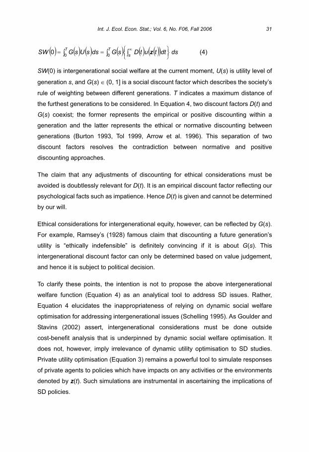
SW(0) is intergenerational social welfare at the current moment, U(s) is utility level of

generation s, and G(s) (0, 1] is a social discount factor which describes the society’s

rule of weighting between different generations. T indicates a maximum distance of

the furthest generations to be considered. In Equation 4, two discount factors D(t) and

G(s) coexist; the former represents the empirical or positive discounting within a

generation and the latter represents the ethical or normative discounting between

generations (Burton 1993, Tol 1999, Arrow et al. 1996). This separation of two

discount factors resolves the contradiction between normative and positive

discounting approaches.

The claim that any adjustments of discounting for ethical considerations must be

avoided is doubtlessly relevant for D(t). It is an empirical discount factor reflecting our

psychological facts such as impatience. Hence D(t) is given and cannot be determined

by our will.

Ethical considerations for intergenerational equity, however, can be reflected by G(s).

For example, Ramsey’s (1928) famous claim that discounting a future generation’s

utility is “ethically indefensible” is definitely convincing if it is about G(s). This

intergenerational discount factor can only be determined based on value judgement,

and hence it is subject to political decision.

To clarify these points, the intention is not to propose the above intergenerational

welfare function (Equation 4) as an analytical tool to address SD issues. Rather,

Equation 4 elucidates the inappropriateness of relying on dynamic social welfare

optimisation for addressing intergenerational issues (Schelling 1995). As Goulder and

Stavins (2002) assert, intergenerational considerations must be done outside

cost-benefit analysis that is underpinned by dynamic social welfare optimisation. It

does not, however, imply irrelevance of dynamic utility optimisation to SD studies.

Private utility optimisation (Equation 3) remains a powerful tool to simulate responses

of private agents to policies which have impacts on any activities or the environments

denoted by z(t). Such simulations are instrumental in ascertaining the implications of

SD policies.


4. INTERGENERATIONAL EQUITY IN SUSTAINABLE DEVELOPMENT

Intergenerational equity in SD is not about efficiency but about conservation of the

basis of human survival.

SD as a global political agenda aims at achieving both poverty alleviation and

environmental sustainability. An underlying recognition is that poverty alleviation

requires economic development while conventional economic development has too

often destroyed the basis of human survival such as rainforests, fertile agricultural

lands or freshwater ecosystems (World Commission on Environment and

Development 1987). In the famous WCED definition of SD, intergenerational equity is

expressed as “without compromising the ability of future generation to meet their own

needs” (World Commission on Environment and Development 1987; p.43). Rapid

destruction of rainforests is regarded as unsustainable not because a decrease in

natural capital may result in intergenerational inefficiency but because we intuitively

fear that it may result in some irreversible catastrophe.

Suppose we can successfully alleviate poverty without undermining the basis of

human survival. Future generations will set their own targets based on their values and

preference system and will pursue those targets. They will not bother whether they can

inherit less wealth, as a total or as any individual elements, than preceding

generations, so long as they can inherit the world free from poverty and fatal

environmental threats to human survival. It is the same as the present generation not

bothering whether previous generations were wealthier than us or not.

This clarification suggests that intergenerational equity in SD is better represented as

certain “survival conditions” rooted in physical facts. A candidate is the maintenance of

integrity of ecosystems that underpin the life-support systems such as sound

hydrological cycle, nutrients cycles, and soil systems. This is obviously a necessary

condition, but not a sufficient condition, to secure the basis of human survival. We

know very little about ecosystems’ behaviour and operationalising this condition is a

real challenge, but an approach based on the concept of ecological resilience appears

to be promising (Common and Perrings 1992, Kojima 2005).

Resilience of a system, after Holling (1973), can be defined as the maximum

perturbation of the system that does not cause the system to leave its original stability


domain (Perrings and Dalmazzone 1997). A candidate of survival conditions based on

this concept is that perturbations in life-support ecosystems caused by development

should be less than the ecosystems’ resilience.6 It must be possible to set certain safe

minimum standards based on the precautionary principle for this purpose, although we

currently have very limited ability to understand behaviours of ecosystems due to

non-linearity, path-dependence, discontinuity, and uncertainty associated with

ecosystems (Perrings et al. 1995). It is well known that many indigenous peoples have

shaped their life style so that they can avoid losing ecosystem resilience. Needless to

say, the more scientific knowledge we have about ecosystem behaviour, the less strict

safe minimum standards we can adopt.

A good example of this approach would be the Kyoto Protocol. Its thrust was the fear of

irreversible catastrophe caused by global warming such as cessation of ocean current

or irreversible changes in ecosystems, in other words, loss of ecosystem resilience.

The Kyoto Protocol demonstrates the ability of the international community to

establish political consensus on safe minimum standards of GHGs emissions for

avoiding such loss of resilience in spite of limited scientific knowledge of climate

change mechanisms and ecosystems’ behaviour under the potential global warming.

There are many other threats to life-supporting ecosystems including desertification,

soil degradation, excessive groundwater exploitation, and so on. Sustainable

development requires establishment of safe minimum standards to maintain resilience

of these ecosystems in parallel with accumulating knowledge about them.

5. CONCLUSIONS

Through examination of basic assumptions underlying intergenerational social welfare

functions based on RCK models, this paper presents an alternative interpretation that

dynamic optimisation in RCK models simply means that our utility level at this moment

is determined not only by current activities and environments but also by future

expectations.

6

For more discussion on this approach, see Kojima (2005).


According to this interpretation, the intergenerational social welfare function based on

RCK models involves a double integral (or a double summation) and consequently it

can accommodate two discount factors; one is a private discount factor representing

our psychological tendency to devalue distant future events, and the other is a social

discount factor representing a weighting rule of intergenerational welfare comparisons

which must be determined by value judgements and through political processes. If

both ethical and empirical discount factors coexist, the seemingly unbridgeable

dispute over choice of discount factor between ethical (normative) and empirical

(positive) approaches disappears. Separation of private and social discount factors

makes it clear that there is no convincing ground to devalue the utility of future

generations (Ramsey 1928).

The above discussion prompts reconsideration of adequate treatment of

intergenerational equity in SD studies. If SD primarily aims at achieving both poverty

alleviation and environmental sustainability, as the Brundtland Report (World

Commission on Environment and Development 1987) claimed, intergenerational

equity in SD is not about efficiency but rather about conservation of the basis of human

survival. Discounting matters only if efficiency is the main concern. This paper claims

that intergenerational equity in SD is better represented as certain “survival conditions”

rooted in physical facts instead of sustainability conditions based on a value

judgement such as discounting. An approach based on an ecological resilience

concept is illustrated as one candidate of such survival conditions.

The alternative treatment of dynamic utility optimisation and intergenerational equity

proposed by this paper is expected to sort out some confusion in sustainable

development literature. For instance it elucidates why there is no convincing way to

incorporate intergenerational equity into cost benefit analysis, which is based on RCK

framework, of long-term environmental problems such as global warming. Large time

scale of global warming is required because of its potential long-run effects on

ecosystem resilience, and such long-term concern can be accommodated by survival

conditions but not by cost benefit based sustainability conditions. Equation 4 and the

proposed ecological resilience approach corroborate the claim that intergenerational

considerations must be done outside cost-benefit analysis (Schelling 1995, Goulder

and Stavins 2002).


As a final conclusion of this paper, it must be emphasised that the mainstream

definition of SD in ecological/environmental economics as eternally non-declining

well-being has an appeal only for the richer portion of the world population. It is high

time for ecological/environmental economics as a discipline to reconsider the original

objectives of SD if it means to address intra- and inter-generational equity issues

responding to the global concern. Although our knowledge about ecosystem

behaviour is limited, the ecological resilience approach illustrated by this paper can be

implemented with the current level of knowledge by setting safe minimum standards

based on the precautionary principle as exemplified by the Kyoto Protocol.

REFERENCES

Aronsson, T., Lofgren, K.G., and Backlund, K., 2004, Welfare Measurement in Imperfect Markets, Edward Elgar, Cheltenham.

Arrow, K.J., Cline, W.R., Maler, K.-G., Munasinghe, M., Squitieri, R. and Stiglitz, J.E., 1996, Intertemporal equity, discounting, and economic efficiency, in Bruce, J.P., Lee, H. and Haites, E.F. (ed.), Climate Change 1995: Economic and Social Dimensions of Climate Change, Cambridge University Press, Cambridge, 129-144.

Arrow, K.J. and Kurz, M., 1970, Public Investment, the Rate of Return, and Optimal Fiscal Policy, Resources for the Future, Baltimore, MD.

Beltratti, A., 1997, Growth with natural and environmental resources, in Carraro, C. and Siniscalco, D. (ed.), New Directions in the Economic Theory of the Environment, Cambridge University Press, Cambridge, 7-42.

Bergson, A., 1938, A reformulation of certain aspects of welfare economics, Quarterly Journal of Economics, 52, 310-334.

Burton, P.S., 1993, Intertemporal preferences and intergenerational equity considerations in optimal resource harvesting, Journal of Environmental Economics and Management, 24, 119-132.

Cass, D., 1965, Optimum growth in an aggregative model of capital accumulation,Review of Economic Studies, 32, 233-240.

Chichilnisky, G., 1996, An axiomatic approach to sustainable development, Social Choice and Welfare, 13, 219-248.

Common, M.S. and Perrings, C.A., 1992, Towards an ecological economics of sustainability, Ecological Economics, 6, 7-34.

Dasgupta, P. and Heal, G.M., 1974, The optimal depletion of exhaustible resource,Review of Economic Studies, Symposium on the Economics of Exhaustible Resources, 3-28.


Gorman, W.M., 1957, Convex indifference curves and diminishing marginal utility,Journal of Political Economy, 65, 40-50.

Goulder, L.H. and Stavins, R.N., 2002, Discounting: an eye on the future, Nature, 419, 673-674.

Holling, C.S., 1973, Resilience and stability of ecological systems, Annual Review of Ecology and Systematics, 4, 1-24.

Kojima, S., 2005, Quantitative Policy Analysis for Sustainable Development in Water-stressed Developing Countries: A Case Study of Morocco, Ph.D. Thesis, University of York, York.

Koopmans, T.C., 1965, On the concept of optimal economic growth, Pontificae Academiae Scientiarum Scripta Varia, 28, 225-300.

Perrings, C., Maler, K.-G., Folke, C., Holling, C.S. and Jansson, B., 1995, Introduction: Framing the problem of biodiversity loss, in Perrings, C., Maler, K.-G., Folke, C., Holling, C.S. and Jansson, B. (ed.), Biodiversity Loss, Cambridge University Press, Cambridge,1-17.

Perrings, C.A. and Walker, B., 1997, Biodiversity, resilience and the control of ecological-economic systems: the case of fire-driven rangelands, Ecological Economics, 22, 73-83.

Ramsey, F.P., 1928, A mathematical theory of saving, Economic Journal, 38, 543-559.

Schelling, T.C., 1995, Intergenerational discounting, Energy Policy, 23, 395-401.

Strotz, R.H., 1956, Myopia and inconsistency in dynamic utility maximisation, Review of Economic Studies, 23, 165-180.

Tol, R.S.J., 1999, Time discounting and optimal emission reduction: an application of FUND, Climate Change, 41, 351-362.

Toman, M.A., Pezzy, J. and Krautkraemer, J., 1995, Neoclassical economic growth theory and "sustainability", in Bromley, D.W. (ed.), Handbook of Environmental Economics, Blackwell, Oxford, 139-165.

World Commission on Environment and Development, 1987, Our Common Future,Oxford University Press, Oxford.


Solid Waste Market Distortions and Recycling

H. BARTELINGS, R.B. DELLINK1 and E.C. VAN IERLAND

Environmental Economics and Natural Resources Group Wageningen University

P.O. Box 8130 6700 EW Wageningen

The Netherlands [email protected]

ABSTRACT

Solid waste management is an important topic in environmental economics, and there is a need for providing better incentives to further optimize the chain of materials and waste. We investigate market distortions caused by flat fee pricing in the solid waste market and we show how flat fee pricing influences households in their decisions to recycle, separate or dispose of rest waste. We develop and apply a general equilibrium model for the solid waste market and describe in detail how market distortions, as a result of flat fee pricing, can be analyzed in an applied general equilibrium framework. A numerical example demonstrates the effects of flat fee pricing on both waste generation and recycling. In the presence of flat fee pricing, the cost of recycling has no impact on the behavior of households, and thus households are not responsive to recycling subsidies. The results show that introducing a unit-based pricing scheme for waste collection can stimulate recycling far more effectively than subsidies and improve the effectiveness of recycling policies.

KEYWORDS: Applied General Equilibrium Modeling; Market distortions, Policies; Recycling; Waste management

JEL classification: D58; H21; Q28

Mathematics Subject Classification 2000: 91B76, 91B32

INTRODUCTION

Governments still fail to achieve a decoupling between waste generation and economic

growth. For example, since 1950, the quantity of waste generated in the Netherlands has

more than tripled, from about 17 Mtonnes in 1950 to about 67 Mtonnes in 2000 (WMC,

2003). The European Environment Agency (EAA, 2000) has demonstrated that waste

generation in the European Union is still coupled with economic growth, making it impossible

1Corresponding author


to pursue economic growth without creating increasingly serious waste management

problems.

Several studies have shown that failure to achieve a decoupling between waste generation

and economic growth can be attributed to flat fee pricing for waste collection (see for

example Miedema, 1983)1. Most studies on the effects of distortions in the solid waste

market have used a partial equilibrium approach. Wertz (1976) was the first to analyze the

effects of a user charge on solid waste disposal. Miedema (1983) analyzed the effects of

other distortionary characteristics of the solid waste market, like virgin material-biased tax

policies, virgin material-biased regulations, and indirect subsidization of virgin materials.

Other empirical studies include Jenkins (1993), Hong et al. (1993), Miranda et al. (1994),

Morris and Holthausen (1994), Sterner and Bartelings (1999), and Kinnaman and Fullerton

(2000). The overall conclusion of these studies is that solid waste generation is sensitive to

user fees; the introduction of user fees can cause a substantial reduction in solid waste

generation, especially if they are combined with programs that enlarge the public awareness

for the solid waste problem.

However, thoughtless construction of waste handling tariffs might not have the desired effect

and can encourage illicit dumping, burning, or other improper disposal. Fullerton and

Kinnaman (1996) estimate that about 28% of the decrease in waste generation may be

caused by increased illegal disposal. Empirical studies, like Jenkins (1993) and Miranda and

Aldy (1998), also report instances of increased illegal dumping. These results, however, are

contradicted by other empirical studies. For example, Miranda et al. (1994), Strahman et al.

(1995), Nestor and Podolsky (1998), Podolsky and Spiegel (1998), Sterner and Bartelings

(1999) and Linderhof et al. (2001) found no significant evidence of increased illegal disposal.

Despite the risk of illegal disposal, the unit-based price is one of the most effective policy

options to provide an incentive to increase prevention and home composting. For instance,

Calcott and Walls (2002) find that a modest disposal charge will always be part of the set of

optimal policy instruments. Shinkuma (2003) argues that even if illegal disposal is an option,

the unit-based pricing system will still provide a second best optimum as long as the price of

recycled material is positive.

In this paper we extend the analysis of the impact of different pricing systems on waste

collection and recycling. In contrast to previous research, we build a general equilibrium

model focusing on the complete product chain from extraction to production to consumption

and finally to recycling and waste treatment. By developing this more complex general

equilibrium model, we can analyze whether policy changes in the end phase of a product

also has an impact on the extraction sector, and production phase of a product, and

consequently on the prices of and demand for consumption goods. Thus we can show the

direct effects of waste policy changes on recycling behavior and solid waste generation and

the indirect effects through price changes and changes in consumption patterns. Inspection

of the indirect effects can also shed light on the importance of using a general equilibrium

approach in comparison to a partial equilibrium framework.


The paper evaluates the effectiveness of unit-based pricing versus a curbside recycling

program, which stimulates recycling by subsidizing recycling efforts. We analyze whether

policies aimed at promoting recycling and waste reduction are more effective under a flat fee

or under unit-based pricing. Policymakers prefer recycling to incineration or landfilling since

recycling will in general have less environmental effects and will help in closing the material

cycle. This is in line with the idea of the waste hierarchy2. Although some studies have

shown that recycling may not be preferred in some cases (see for example Barrett and

Lawlor, 1997), we will not address this issue.

The paper is structured as follows: Section 2 describes the model and shows how both flat

fee pricing and unit-based pricing can be included in an applied general equilibrium model.

Section 3 presents a numerical example in which the consequences of flat fee pricing versus

unit based pricing mechanisms and the possibilities to promote recycling are analyzed. Data

used in this example are based on the Netherlands in 1996. The model is constructed,

however, in such a way that results can be generalized to other countries. Section 4

concludes.

DESCRIPTION OF THE MODEL

1.1 General description of the AGE model

For studying the various waste management options we develop an applied general

equilibrium model for a national economy, including a solid waste market. Consumers

maximize utility and producers maximize profit. An applied general equilibrium model can be

solved in various ways, also called formats3. In this paper the Negishi-format (as proposed

by Negishi, 1972) is chosen as the preferred tool for building an applied general equilibrium

model. One of the advantages of the Negishi format is the relative ease with which non-

convexities, such as a flat fee-pricing scheme, can be implemented (see also Ginsburgh and

Keyzer, 1997).

1.2 General introduction to the model structure

In the model, two types of actors are distinguished: consumers and firms. Consumers buy

goods and services and supply production factors; firms produce goods and services and

use both production factors and intermediate goods as inputs to production. We distinguish

two types of consumers -private households and the government- and eight types of

producers, each producing one unique good. These producers are: (1) a producer of

extraction services producing virgin material; producers of (2) agricultural goods, (3)

industrial goods and (4) commercial services; (5) a producer of waste recycling services; (6)

a producer of waste collection services and producers of (7) waste incineration services and

(8) waste landfilling services. The life cycle of materials for the hypothetical economy is

shown in Figure 1.


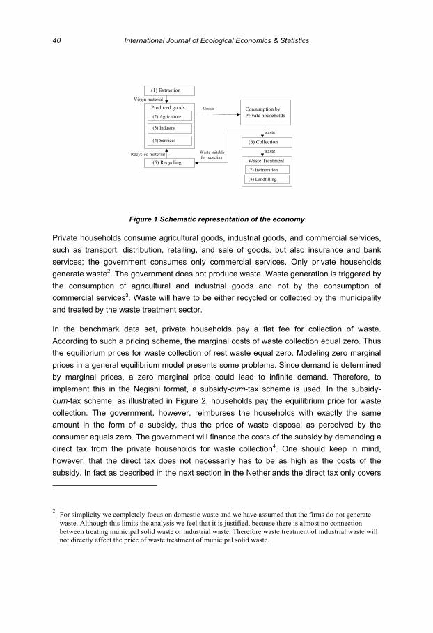
(1) Extraction

Produced goods

Virgin material

Consumption by

Private households

(5) Recycling

Recycled material

(6) Collection

Waste Treatment

(7) Incineration

(8) Landfilling

(2) Agriculture

(4) Services

(3) Industry

Goods

Waste suitable

for recycling

waste

waste

Figure 1 Schematic representation of the economy

Private households consume agricultural goods, industrial goods, and commercial services,

such as transport, distribution, retailing, and sale of goods, but also insurance and bank

services; the government consumes only commercial services. Only private households

generate waste2. The government does not produce waste. Waste generation is triggered by

the consumption of agricultural and industrial goods and not by the consumption of

commercial services3. Waste will have to be either recycled or collected by the municipality

and treated by the waste treatment sector.

In the benchmark data set, private households pay a flat fee for collection of waste.

According to such a pricing scheme, the marginal costs of waste collection equal zero. Thus

the equilibrium prices for waste collection of rest waste equal zero. Modeling zero marginal

prices in a general equilibrium model presents some problems. Since demand is determined

by marginal prices, a zero marginal price could lead to infinite demand. Therefore, to

implement this in the Negishi format, a subsidy-cum-tax scheme is used. In the subsidy-

cum-tax scheme, as illustrated in Figure 2, households pay the equilibrium price for waste

collection. The government, however, reimburses the households with exactly the same

amount in the form of a subsidy, thus the price of waste disposal as perceived by the

consumer equals zero. The government will finance the costs of the subsidy by demanding a

direct tax from the private households for waste collection4. One should keep in mind,

however, that the direct tax does not necessarily has to be as high as the costs of the

subsidy. In fact as described in the next section in the Netherlands the direct tax only covers

2For simplicity we completely focus on domestic waste and we have assumed that the firms do not generate

waste. Although this limits the analysis we feel that it is justified, because there is almost no connection

between treating municipal solid waste or industrial waste. Therefore waste treatment of industrial waste will

not directly affect the price of waste treatment of municipal solid waste.


about 95% of the costs of waste collection. Implicitly this means that the government is

subsidizing part of the costs of waste collection.

Private households

Municipalityas collectorof waste

price subsidyflat fee

Real money transfer

Hypothetical money transfer

collection

services

Transfer ofgoods andservices

waste

Figure 2 The subsidy-cum-tax scheme

The model used in this paper describes a closed economy. Allowing import and export of

waste and goods will hardly affect the results because we are focusing on the effects policy

measures have on the generation of household waste. Households in this case make the

decision whether or not to recycle waste. Both recycled waste and rest waste are collected

by the municipality. The households do not have the option of transporting waste to a

treatment center themselves. Modeling an open economy will only have an impact due to a

larger supply of waste extensive products. However, it can be expected that these effects

will be minimal as the expected waste prevention due to the introduction of unit-based

pricing or recycling subsidies is minimal. Furthermore, international trade in waste is still

rather uncommon.

1.3 Description of the model

In the Negishi format, total welfare is maximized subject to the relevant balance constraints

and production possibilities (Ginsburgh and Keyzer, 1997). The total welfare function is

shown in equation 2.1. Total welfare (TWF) is determined by the sum of the weighted utilities

(ui) of all consumers (i=1,...,I) . Consumers derive utility from consumption of produced

goods (xig) where g=1,...,G denotes the produced goods. The utility of each consumer is

weighted by a factor i, the so-called Negishi weights5.

,

,

( ) max ( )

0 , ,

i i i g

i

i g j

TWF u x TW

x all i y all j

(2.1)

3Production of commercial services could lead to generation of waste. Consumption of these services, however,

will not lead to substantial amounts of waste generation due to the specific nature of commercial services;

therefore, we have omitted this from the model.


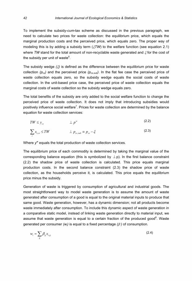
To implement the subsidy-cum-tax scheme as discussed in the previous paragraph, we

need to calculate two prices for waste collection: the equilibrium price, which equals the

marginal production costs and the perceived price, which equals zero. The proper way of

modeling this is by adding a subsidy term ( TW) to the welfare function (see equation 2.1)

where TW stand for the total amount of non-recyclable waste generated and for the cost of

the subsidy per unit of waste6.

The subsidy wedge ( ) is defined as the difference between the equilibrium price for waste

collection (pcs) and the perceived price (pcs,sub). In the flat fee case the perceived price of

waste collection equals zero, so the subsidy wedge equals the social costs of waste

collection. In the unit-based price case, the perceived price of waste collection equals the

marginal costs of waste collection so the subsidy wedge equals zero.

The total benefits of the subsidy are only added to the social welfare function to change the

perceived price of waste collection. It does not imply that introducing subsidies would

positively influence social welfare7. Prices for waste collection are determined by the balance

equation for waste collection services:

w

csTW y p (2.2)

, ,i cs cs sub cs

i

x TW p p (2.3)

Where yw equals the total production of waste collection services.

The equilibrium price of each commodity is determined by taking the marginal value of the

corresponding balance equation (this is symbolized by p). In the first balance constraint

(2.2) the shadow price of waste collection is calculated. This price equals marginal

production costs. In the second balance constraint (2.3) the shadow price of waste

collection, as the households perceive it, is calculated. This price equals the equilibrium

price minus the subsidy.

Generation of waste is triggered by consumption of agricultural and industrial goods. The

most straightforward way to model waste generation is to assume the amount of waste

generated after consumption of a good is equal to the original material inputs to produce that

same good. Waste generation, however, has a dynamic dimension; not all products become

waste immediately after consumption. To include this dynamic aspect of waste generation in

a comparative static model, instead of linking waste generation directly to material input, we

assume that waste generation is equal to a certain fraction of the produced good8. Waste

generated per consumer (wi) is equal to a fixed percentage ( ) of consumption.

,i g i g

g

w x (2.4)


It is assumed that all waste generated is either collected (xcs) or recycled (xr), the model

does not take into account illegal disposal of any kind. ´Environmental awareness´ may

affect the choices of households regarding recycling, but this is not explicitly considered in

the model, due to a lack of empirical information.

, ,i r i cs ix x w (2.5)

All firms produce commodities yj within their given production set Yj. The production set for

each of the firms in the model is given by a nested CES production function that depends on

the input of capital (k), labor (l), virgin material (qv), recycled material (qr) and intermediate

inputs (qg).

Finally, a common requirement in applied general equilibrium models is that demand should

equal supply for each commodity. This is ensured in various balance constraints9.

A NUMERICAL EXAMPLE

The model discussed above is applied in a numerical example with stylized data for the

Netherlands. The economic data used in the numerical example are based on the economy

in the Netherlands in 1996 (Statistics Netherlands, 1998). We have chosen to use data from

1996 because at that time the Netherlands had hardly started with modern waste

management policies. After 1996, they introduced landfilling taxes, landfilling bans, waste

separation, and municipalities started experimenting with unit-based pricing. By using data

from 1996 we do not have to separate the effects of these policies on the choice between

recycling, landfilling, and incineration from the effects of new policies we want to examine.

1.4 Parameter values used in numerical example

Parameter values are based on the accounting matrix displayed in Table 1, which describes

the initial equilibrium. Supply, i.e. producer outputs and consumer endowments, are given

positive values; demand, i.e. producer inputs and consumption, are given negative values10.

All prices are normalized to unity except the price of waste collection. As explained in section

2, waste collection basically has two prices: a perceived price and a social price. The

perceived price equals the total fee divided by the total demand for waste collection. The

social price equals the total fee plus the total amount paid by the government for waste

collection divided by the total demand. We have chosen to normalize the perceived price for

waste collection, which means that the social price for waste collection (which is shown in

Table 1) is higher than unity.

Government expenditure is kept constant in the model at the benchmark level to avoid

modeling problems concerning public expenditure incidence. When the income of the

government changes in the model due to policy measures, the model simulates the private

households compensating the government through a lump-sum transfer.


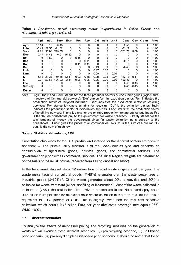
Table 1 Benchmark social accounting matrix (expenditures in Billion Euros) and standardized prices (last column).

Agri Indu Serv Extr Rm Rec Col Incin Land Cons Gov C-sum Price

Agri 18.18 -8.18 -0.45 0 0 0 0 0 0 -9.55 0 0 1.00Indu -5.45 99.55 -21.82 0 0 0 0 0 0 -72.27 0 0 1.00Serv -1.82 -25.91 239.55 0 0 0 0 0 0 -202.73 -9.09 0 1.00Extr -0.45 -14.45 -0.91 15.82 0 0 0 0 0 0 0 0 1.00Rm 0 -1.82 0 0 0.18 0 0 0 0 0 0 0 1.00Rec 0 0 0 0 0 0.11 0 0 0 -0.11 0 0 1.00Rw 0 0 0 0 -0.11 0.11 0 0 0 0 0 0 1.00Col 0 0 0 0 0 0 0.43 0 0 -0.43 0 0 1.05Incin 0 0 0 0 0 0 -0.27 0.27 0 0 0 0 1.00Land 0 0 0 0 0 0 -0.09 0 0.09 0 0 0 1.00K -8.18 -21.27 -89.55 -12.41 -0.02 -0.18 -0.05 -0.23 -0.07 122.73 9.11 0 1.00L -2.27 -29.55 -126.82 -3.41 -0.05 -0.05 -0.05 -0.05 -0.02 162.36 0 0 1.00Fee 0 0 0 0 0 0 0 0 0 -0.43 0.43 0 1.00Subsidy 0 0 0 0 0 0 0 0 0 0.45 -0.45 0 1.00

R-sum 0 0 0 0 0 0 0 0 0 0 0 0

Note: ‘Agri’, ‘Indu’ and ‘Serv’ stands for the three producer sectors of consumer goods (Agriculture, Industry and Commercial services); ‘Extr’ stands for the extraction sector; ‘Rm’ indicates the production sector of recycled material; ‘Rec’ indicates the production sector of recycling services; ‘Rw’ stands for waste suitable for recycling; ‘Col’ is the collection sector; ‘Incin’ indicates the production sector of incineration services; ‘Land’ indicates the production sector of landfilling services; K and L stand for the primary production factors capital and labor; Fee is the flat fee households pay to the government for waste collection; Subsidy stands for the total amount of money the government gives for waste collection as a subsidy to the households; ‘Price’ gives the prices of all commodities; ‘R-sum’ is the sum of a column; ‘C-sum’ is the sum of each row.

Source: Statistics Netherlands, 1998

Substitution elasticities for the CES production functions for the different sectors are given in

appendix A. The private utility function is of the Cobb-Douglas type and depends on

consumption of agricultural goods, industrial goods, and commercial services. The

government only consumes commercial services. The initial Negishi weights are determined

on the basis of the initial income (received from selling capital and labor).

In the benchmark dataset about 12 million tons of solid waste is generated per year. The

waste percentage of agricultural goods ( =46%) is smaller than the waste percentage of

industrial goods ( =69%)11. Of the waste generated about 20% is recycled and 80% is

collected for waste treatment (either landfilling or incineration). Most of the waste collected is

incinerated (75%); the rest is landfilled. Private households in the Netherlands pay about

0.43 billion Euro per year for municipal solid waste collection in the form of a flat fee, this is

equivalent to 0.1% percent of GDP. This is slightly lower than the real cost of waste

collection, which equals 0.45 billion Euro per year (the costs coverage rate equals 95%,

WMC, 1997).

1.5 Different scenarios

To analyze the effects of unit-based pricing and recycling subsidies on the generation of

waste we will examine three different scenarios: (i) pro-recycling scenario, (ii) unit-based

price scenario, (iii) pro-recycling plus unit-based price scenario. It should be noted that these


scenarios are not particularly meant as policy recommendations, but they are used to show

how distortions caused by flat fee pricing influence household behavior. The results of each

of these scenarios are compared to the results of the benchmark case. The benchmark case

is described by the data presented in section 1.4 and contains the flat fee pricing scheme.

In the first scenario, recycling is promoted by introducing a subsidy on recycling. Due to the

introduction of a subsidy, recycling will be 30% less expensive. The flat fee-pricing scheme

is not changed. This policy is labeled ‘pro-recycling scenario’.

In the second scenario the flat fee-pricing scheme is replaced by a unit-based pricing

scheme. This policy is labeled ‘unit-based price scenario’. In this scenario the households

pay the equilibrium price for waste collection equal to the costs of producing waste collection

services12.

In the third scenario both the variable pricing scheme and the recycling subsidy are

introduced. By comparing these results with the results of scenario 1, we will show how the

effectiveness of the recycling subsidy is affected by the flat fee scheme. This scenario is

labeled ‘pro-recycling plus unit-based price scenario’.

1.6 Results

1.6.1 Pro-recycling scenario

In the first policy scenario, the price of recycling is reduced by introducing a subsidy on

recycling efforts.

Table 2 The main variables for the ‘Pro-recycling scenario’ as compared to the ‘Benchmark case’ (expenditures in Billion Euro) and the percentage change

Benchmark Pro-recycling % change

Demand by private households

Agricultural good 9.55 9.55 0.0%

Industrial good 72.27 72.27 0.0%

Commercial services 202.73 202.73 0.0%

Recycling services 0.11 0.11 0.0%

Waste collection 0.43 0.43 0.0%

Recycled material 0.18 0.18 0.0%

Prices







Utility private households 140.81 140.81 0.0%


Table 2 shows the changes in the demand for goods and services and the demand for

recycling services and waste collection services. The demand for recycling services is not

affected by the lower price for recycling services. This is an expected result because if

households have the choice between collection and recycling services, the rational

consumer will chose collection, which is free. So a lower price for recycling services will not

affect the demand for these services as long as this price is larger than zero.

Since the expenditure of the government is kept constant at benchmark level within the

model (see section 3.1), the government receives a small lump-sum transfer from the private

households to compensate for the extra costs of the subsidy. Therefore the policy measure

has no impact on the income of the households and consumption and utility are not affected.

1.6.2 Unit-based price scenario

The second scenario simulates the introduction of a unit-based pricing scheme for waste

collection. Households now pay the equilibrium price for waste collection in which more

generation of waste means more costs to private households for waste collection.

The results of this scenario are shown in Table 3. In the benchmark scenario the flat fee

covered about 95% of the costs of waste collection, the government financed the remaining

5%. In this scenario the private households bear the full costs of waste collection, thus

without intervention the expenditure of the government would increase. However, to avoid

problems such as public expenditure incidence, we assume that government expenditure is

constant. Thus, the government gives a positive lump-sum transfer to the private households

(equal to 5% of the costs of waste collection). Private households now bear the full cost of

waste collection, but because of the positive lump-sum transfer there is compensating

change in the income they can spend on consumer goods. Therefore social welfare does not

increase in this scenario.

Because recycling is now slightly less expensive then waste collection, households start to

recycle more waste. This increases the demand for recycling services, which in turn causes

the price of recycling services to rise. In the equilibrium solution the price of recycling

services is again equal to the price of collection services. Recycling increases slightly (6.6%)

and thus the price of recycled material decreases slightly (-3%). This changes the choice

producers make between the use of recycled material versus virgin material, and the

demand for recycled material increases with 5.5 percent.

The results suggest that introducing a unit-based price may give private households both an

incentive to prevent generation of waste and to recycle waste. Since the costs of waste

collection have increased, households have an incentive to prevent waste generation by

substituting the waste intensive goods (agricultural and industrial goods) for the waste

extensive good (commercial services). Households may also have an incentive to recycle

more waste, since recycling in our specification is somewhat cheaper than waste collection.


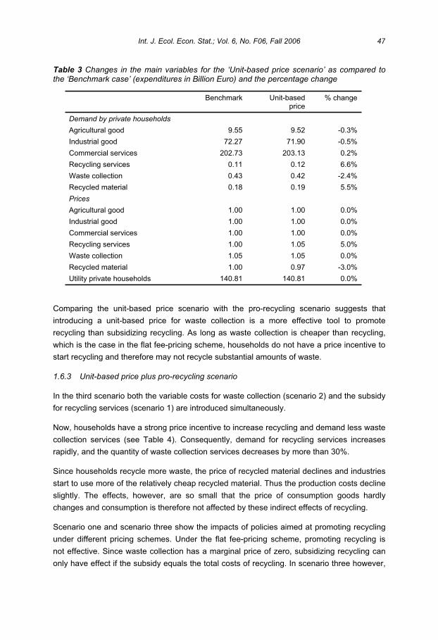
Table 3 Changes in the main variables for the ‘Unit-based price scenario’ as compared to the ‘Benchmark case’ (expenditures in Billion Euro) and the percentage change

Benchmark Unit-based price

% change


Agricultural good 9.55 9.52 -0.3%

Industrial good 72.27 71.90 -0.5%



Waste collection 0.43 0.42 -2.4%


Prices






Recycled material 1.00 0.97 -3.0%


Comparing the unit-based price scenario with the pro-recycling scenario suggests that

introducing a unit-based price for waste collection is a more effective tool to promote

recycling than subsidizing recycling. As long as waste collection is cheaper than recycling,

which is the case in the flat fee-pricing scheme, households do not have a price incentive to

start recycling and therefore may not recycle substantial amounts of waste.

1.6.3 Unit-based price plus pro-recycling scenario

In the third scenario both the variable costs for waste collection (scenario 2) and the subsidy

for recycling services (scenario 1) are introduced simultaneously.

Now, households have a strong price incentive to increase recycling and demand less waste

collection services (see Table 4). Consequently, demand for recycling services increases

rapidly, and the quantity of waste collection services decreases by more than 30%.

Since households recycle more waste, the price of recycled material declines and industries

start to use more of the relatively cheap recycled material. Thus the production costs decline

slightly. The effects, however, are so small that the price of consumption goods hardly

changes and consumption is therefore not affected by these indirect effects of recycling.

Scenario one and scenario three show the impacts of policies aimed at promoting recycling

under different pricing schemes. Under the flat fee-pricing scheme, promoting recycling is

not effective. Since waste collection has a marginal price of zero, subsidizing recycling can

only have effect if the subsidy equals the total costs of recycling. In scenario three however,


the amount of waste generated goes down. More waste is recycled and less waste is

collected, incinerated, or landfilled. Comparing these scenarios shows that in our simplified

economy the flat fee for waste collection causes a serious market distortion. Because of the

flat fee pricing system, the price of recycling has no impact on the behavior of households

and thus households are not responsive to recycling subsidies.

Table 4 Changes in the main variables for the ‘Unit-based price and pro-recycling scenario’ as compared to the ‘Benchmark case’ (expenditures in Billion Euro) and the percentage change.

Benchmark Pro-recycling & unit-based price

% change


Agricultural good 9.55 9.53 -0.2%

Industrial good 72.27 71.94 -0.5%



Waste collection 0.43 0.29 -32.4 %


Prices






Recycled material 1.00 0.68 -32.0%


DISCUSSION

We have demonstrated how an applied general equilibrium model simulating the solid waste

market and incorporating market distortions can be built. Since one of the characteristics of

the waste market is the flat fee-pricing scheme for waste collection, it is important to realize

that the actual price for waste collection that the households perceive is equal to zero.

Special attention, therefore, has been given to modeling goods with a zero price. Such a

market distortion has strong effects on the results of the model. This was shown in the

application of the model in a numerical example using 1996 data for the Netherlands.

By modeling the complete product chain we can investigate not only the direct effects of unit-

based pricing and recycling subsidies, but also the indirect effects through the prices of

recycled material. One should keep in mind, however, that unit-based pricing may increase

illegal dumping of waste (cf. Fullerton and Kinnaman, 1996). We abstracted from the costs


associated with dumping as empirical studies suggest that this is a minor problem; in

principle, social costs associated with illegal dumping can and should be accounted for in the

unit-based price of waste collection. Furthermore, our approach abstracts from any impact of

environmental awareness or other links between waste generation and welfare. These links

are complex and virtually impossible to specify in an applied model such as ours.

Looking at the scenario where the unit-based pricing is combined with the recycling subsidy,

we observe that due to a price decrease of recycled material, producers start to use far more

recycled material. The decrease of production costs is, however, only slight and therefore we

do not see any decrease in the prices of consumption goods and commercial services due to

increased recycling efforts. Thus there are no significant indirect effects on the consumption

pattern. This result implies that for this specific policy analysis, partial equilibrium analysis

can provide relatively good approximations of the economic impacts of the policy.

The direct effects of unit-based pricing and recycling subsidies on household behavior are

more pronounced. The modeling results suggest that a flat fee-pricing scheme for waste

collection reduces the economic incentives to recycle. As long as a flat fee-pricing scheme is

used, private households do not have economic incentives to reduce solid waste generation

and for that reason will show little tendency to recycle. Even without taking into account the

environmental gain of less waste it is effective to introduce unit-based pricing as it does not

negatively affect the welfare of the society. Making recycling more attractive by subsiding

recycling efforts will not result in substantially less solid waste generation as long as the

price of recycling are greater than zero. Only if policies for promoting recycling are combined

with a unit-based pricing scheme for waste collection will these policies be effective.

1 In a flat fee pricing system municipalities charge a fixed price for waste collection independent of the

amount of waste actually generated.

2 The waste hierarchy is a qualitative ranking of waste management or disposal practices. According

to the waste hierarchy, the optimal waste treatment option is prevention followed by recycling and re-

use, composting, incineration and landfilling, which is the least preferred way of dealing with waste.

3 The formats are: 1) Computable general equilibrium format, 2) Negishi format, 3) Open economy

format, and 4) Full format. Each of these formats has its strengths and weaknesses, for more

information see Ginsburgh and Keyzer (1997). It must be stressed however that a format is just a way

to solve a general equilibrium model. Each of the four formats will find the same equilibrium solution

for the defined problem.

4 A direct tax influences the income of the consumer but does not influence the consumption pattern.

5 In the Negishi format, the equilibrium solution is found with the help of an iterative process. Given

initial values for the Negishi-weights based on the income of a consumer, the model is solved and

prices for each commodity are calculated as shadow prices. Subsequently, the budget constraint for

each consumer is checked. If one or more consumers in the model spend more or less than their


income, the Negishi weight for that consumer is adjusted. The model is then solved again with the

adjusted Negishi-weights. The process continues until the budget constraints of all consumers hold.

See for more information Negishi (1972) or Ginsburgh and Keyzer (1997).

6 See Ginsburgh and Keyzer (1997) for more details on this procedure.

7 If the model were written in another format, the subsidy would not have to be made explicit in the

welfare function. Note that optimal prices and quantities calculated by the model do not depend on the

format chosen.

8 Implicitly this means that part of the used material will accumulate in the stock of durable goods.

Therefore at any given moment of time the material inflow need not be equal to the material outflow.

9 A more extensive description of the model can be found in Bartelings (2003).

10 The column of each producer sums to zero to ensure that the zero profit condition holds (value of

input equals value of output). The column of each consumer sums to zero to ensure that the budget

constraint holds. Each row must sum to zero to ensure that the market clears (total demand must

equal total supply for each commodity).

11 Waste percentage is defined as kg waste present in kg good.

12 Note that the households in this scenario pay the full price for waste collection, while in the

benchmark case the flat fee covers only 95% of the costs (see section 3.1). The two scenarios are

comparable, however, because we assume that government expenditure is constant. Therefore the

government will be compensated for the differences between the flat fee revenues and the real costs

of waste collection through a lump-sum transfer.


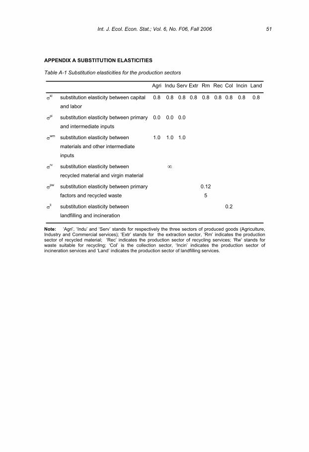
APPENDIX A SUBSTITUTION ELASTICITIES

Table A-1 Substitution elasticities for the production sectors

Agri Indu Serv Extr Rm Rec Col Incin Land

kl substitution elasticity between capital

and labor

0.8 0.8 0.8 0.8 0.8 0.8 0.8 0.8 0.8

pi substitution elasticity between primary

and intermediate inputs

0.0 0.0 0.0

wm substitution elasticity between

materials and other intermediate

inputs

1.0 1.0 1.0

rv substitution elasticity between

recycled material and virgin material

pw substitution elasticity between primary

factors and recycled waste

0.12

5

li substitution elasticity between

landfilling and incineration

0.2

Note: ‘Agri’, ‘Indu’ and ‘Serv’ stands for respectively the three sectors of produced goods (Agriculture, Industry and Commercial services); ‘Extr’ stands for the extraction sector, ‘Rm’ indicates the production sector of recycled material; ‘Rec’ indicates the production sector of recycling services; ‘Rw’ stands for waste suitable for recycling; ‘Col’ is the collection sector, ‘Incin’ indicates the production sector of incineration services and ‘Land’ indicates the production sector of landfilling services.


APPENDIX B DEFINITION OF INDICES, PARAMETERS, AND VARIABLES

Indices

Label Entries Description

g 1,...,3 produced goods (agriculture, industry, commercial services)

i 1,2 consumers (households, government)

j 1,...,8 produced goods and services

z 1,...,10 commodities (including produced goods, services, capital and labor)

Parameters in model specification

Symbol Description

Negishi weight

waste percentage kl substitution elasticity between labor and capital qm substitution elasticity between materials and other intermediate inputs rv substitution elasticity between recycled material and virgin material

pr substitution elasticity between primary factors and recycled waste il substitution elasticity between landfilling and incineration

subsidy wedge

F flat fee for waste collection

LST lump-sum transfer to keep income of government constant

K endowment of capital

L endowment of labor

P price

pt price including subsidy

M0 initial income

Variables in model specification

Symbol Description

k capital use

l labor use

y production

TW total demand for waste collection services

TWF total welfare

u utility

W total generation of waste

x consumption

q Use intermediate goods

Xr total production of recyclable waste

M Income


Appendix C Model specification

In the Negishi format total welfare is maximized given constraints of production sets and balance equations. The total welfare function depends on the weighted utility of the individual consumers:

,

,

( ) max ( )

0, 0, 0 ,

i i i g

i

i g i i j

TWF u x TW

x w r all i y all j

(C.1)

Subject to production function of goods and collection services:

j jy Y for all j (C.2)

, , ,min{ ( , ; ), ( , ( , ; ); )}

, ,

kl w qm

j j j j j g j v j rY A CES k l CES q CES q q

for j agri indu serv

(C.3)

{ ( , ; ), ; } kl pr

j j j j rY A CES CES k l X for j rm (C.4)

, ,min{ ( , ; ), ( , ; )}

kl il

j j j j j is j lsY A CES k l CES q w

for j cs

(C.5)

( , ; ) , ,kl

j j j jY A CES k l for j extr incin land (C.6)

And balance constraints:

, ,i j j1 j j j

i j1

x q y p for all j except col

j1 j

(C.7)

j k

i

j i

k K p (C.8)

j l

i

j i

l L p (C.9)

,i cs cs,sub

i

x TW p (C.10)

cs csTW y p (C.11)

Equations waste generation :

,i g i g

g

w x (C.12)

r w

i i ix x w (C.13)

Negishi weights are determined such that the budget constraint holds for every consumer:

, , ,( ) k lig i g rs i rs cs i cs i i i

g i

i

Mp x p x p x F LST p K p L

M

for i=cons

(C.14)

,

k

g i g i i

g

p x TW p K F LST for i=gov (C.15)

,( )0 k

gov gov i i cs

i i

LST M p K F x (C.16)


REFERENCES

Barrett, A. and Lawlor, J., 1997, Questioning the Waste Hierarchy: The Case of a Region with a Low Population Density, Journal of Environmental Planning and Management, 40, 19-36.

Bartelings, H., 2003, Municipal Solid Waste Management Problems: An Applied General Equilibrium Analysis, PhD thesis, Wageningen University, Wageningen.

Calcott, P. and Walls, M., 2002, Waste, recycling and design for the environment: roles for markets and policy instruments, Resources for the Future Discussion Paper 00-30REV, Resources for the future, Washington.

EAA, 2000, Indicator fact sheet signals 2001 – chapter waste, European Environment Agency, Copenhagen.

Fullerton, D. and Kinnaman, T.C., 1996, Household demand for garbage and recycling collection with the start of a price per bag, American Economic Review, 86, 971-984.

Ginsburgh, V. and Keyzer, M., 1997, The structure of applied general equilibrium models, The MIT Press, London.

Hong, S.R., Adams, M., and Love, H.A., 1993, An economic analysis of household recycling of solid waste: the case of Portland, Oregon Journal of Environmental Economics and Management, 25, 136-146.

Kinnaman, T.C. and Fullerton, D., 2000, Garbage and recycling with endogenous local policy, Journal of Urban Economics, 48, 419-442.

Linderhof, V., Kooreman, P., Allers, M., and Wiersma, D., 2001, Weight-Based Pricing in the Collection of Household Waste; the Oostzaan Case, Resource and Energy Economics, 23, 359-371.

Jenkins, R.R., 1993, The economics of solid waste reduction, the impact of users fees,Edward Elgar, Aldershot.

Miedema, A.K., 1983, Fundamental economic comparisons of solid waste policy options, Resources and Energy, 5, 21-43.

Miranda, M.L., Everett, J.W., Blume, D. and Barbeau, Jr. A.R., 1994, Market-basedincentives and residential municipal solid waste, Journal of Policy Analysis and Management, 13, 681-698.

Miranda, M.L. and Aldy, J.E., 1998, Unit Pricing of residential municipal solid waste: lessons from nine case study communities, Journal of Environmental Management, 52, 79-93.

Morris, G.E. and Holthausen, D.M., 1994, The Economics of Household Solid Waste Generation and Disposal, Journal of Environmental Economics and Management, 26, 215-234.

Negishi, T., 1972, General equilibrium theory and international trade, North-Hollandpublishing company, Amsterdam.


Nestor, D.V. and Podolsky, M.J., 1998, Assessing incentive-based environmental policies for reducing household waste disposal, Contemporary Economic Policy, 16, 27-39.

Podolsky, M.J. and Spiegel, M., 1998, Municipal waste disposal: unit-pricing and recycling opportunities, Public Works Management and Policy, 3, 27-39.

Shinkuma, T., 2003, On the second-best policy of household’s waste recycling,Environmental and Resource Economics, 24, 77-95.

Statistics Netherlands, 1998, National accounts of the Netherlands, Statistics Netherlands, Voorburg.

Sterner, T. and Bartelings, H., 1999, Household waste management in a Swedish municipality: determinants of waste disposal, recycling and composting,Environmental and Resource Economics, 13, 473-491.

Strathman, J.G., Rufolo, A.M., and Mildner, G.C.S., 1995, The Demand for Solid Waste Disposal, Land Economics, 71, 57-64.

Wertz, K.L., 1976, Economic factors influencing household production of refuse,Journal of Environmental Economics and Management, 2, 263-272.

WMC, 1997, Waste treatment in the Netherlands 1996 (in Dutch), WMC 1997-09, Waste Management Council, Utrecht.

WMC, 2003, National waste management plan 2002-2012 (in Dutch), Waste Management Council, Utrecht.


How extreme events can affect a seemingly stabilized population: a stochastic rendition of Ricker’s model

S. Bhattacharya1, S. Malakar2 and F. Smarandache3

1Department of Business Administration Alaska Pacific University, U.S.A.

E-mail: [email protected]

2Department of Chemistry and Biochemistry University of Alaska, U.S.A.

3Department of Mathematics University of New Mexico, U.S.A.

Abstract

Our paper computationally explores Ricker’s predator satiation model with the objective of studying how the extinction dynamics of an animal species having a two-stage life-cycle is affected by a sudden spike in mortality due to an extraneous extreme event. Our simulation model has been designed and implemented using sockeye salmon population data based on a stochastic version of Ricker’s model; with the shock size being reflected by a sudden reduction in the carrying capacity of the environment for this species. Our results show that even for a relatively marginal increase in the negative impact of an extreme event on the carrying capacity of the environment, a species with an otherwise stable population may be driven close to extinction

Key words: Ricker’s model, extinction dynamics, extreme event, Monte Carlo simulation

Mathematics Subject Classification 2000: 65C05, 92D25

JEL classification: C15, Q59

Background and research objective

PVA approaches do not normally consider the risk of catastrophic extreme events

under the pretext that no population size can be large enough to guarantee survival

of a species in the event of a large-scale natural catastrophe. [1] Nevertheless, it is

only very intuitive that some species are more “delicate” than others; and although

not presently under any clearly observed threat, could become threatened with

extinction very quickly if an extreme event was to occur even on a low-to-moderate

scale. The term “extreme event” is preferred to “catastrophe” because catastrophe


usually implies a natural event whereas; quite clearly; the chance of man-caused

extreme events poses a much greater threat at present to a number of animal

species as compared to any large-scale natural catastrophe.

An animal has a two-stage life cycle when; in the first stage, newborns become

immature youths and in the second stage; the immature youths become mature

adults. Therefore, in terms of the stage-specific approach, if Yt denotes the number

of immature young in stage t and At denotes the number of mature adults, then the

number of adults in year t + 1 will be some proportion of the young, specifically those

that survive to the next (reproductive) stage. Then the formal relationship between

the number of mature adults in the next stage and the number of immature youths at

present may be written as follows:

At + 1 = Yt

Here is the survival probability, i.e. it is the probability of survival of a youth to

maturity. The number of young next year will depend on the number of adults in t:

Yt + 1 = f (At)

Here f describes the reproduction relation between mature adults and next year’s

young.

This is a straightforward system of simultaneous difference equations which may be

analytically solved using a variation of the cobwebbing approach. [2] The solution

process begins with an initial point (Y1, A1) and iteratively determines the next point

(Y2, A2). If predator satiation is built into the process, then we simply end up with

Ricker’s model:

Yt + 1 = Ate–At/K

Here is the maximum reproduction rate (for an initial small population) and K is the

population size at which the reproduction rate is approximately half its maximum [3].

Putting = 1/K we can re-write Ricker’s equation as follows:

Yt + 1 = Ate– At


It has been shown that if (Y0, A0) lies within the first of three possible ranges, (Yn, An)

approaches (0, 0) in successive years and the population becomes extinct. If (Y0, A0)

lies within the third range then (Yn, An) equilibrate to a steady-state value of (Y*, A*).

Populations that begin with (Y0, A0) within the second range oscillate between (Y*, 0)

and (0, A*). Such alternating behavior indicates one of the year classes, or cohorts,

become extinct while the other persists i.e. adult breeding stock appear only every

other year. Thus the model reveals that three quite different results occur depending

initially only on the starting sizes of the population and its distribution among the two

stages. [4]

We use the same basic model in our research but instead of analytically solving the

system of difference equations, we use the same to simulate the population

dynamics as a stochastic process implemented on an MS-Excel spreadsheet. Rather

than using a closed-form equation like Ricker’s model to represent the functional

relationship between Yt + 1 and At, we use a Monte Carlo method to simulate the

stage-transition process within Ricker’s framework; introducing a massive

perturbation with a very small probability in order to emulate a catastrophic event.[5]

Conceptual framework

We have a formulated a stochastic population growth model with an inbuilt capacity

to generate an extreme event based on a theoretical probability distribution. The

non-stochastic part of the model corresponds to Ricker’s relationship between Yt + 1

and At. The stochastic part has to do with whether or not an extreme event occurs at

a particular time point. The gamma distribution has been chosen to make the

probability distribution for the extreme event a skewed one as it is likely to be in

reality. Instead of analytically solving the system of simultaneous difference

equations iteratively in some variation of the cobwebbing method, we have used

them in a spreadsheet model to simulate the population growth over a span of ten

time periods.

We apply a computational methodology whereby the initial number of immature

young is hypothesized to either attain the expected number predicted by Ricker’s

model or drastically fall below that number at the end of every stage, depending on

whether an extraneous extreme event does not occur or actually occurs. The


mortalities as a result of an extreme event at any time point is expressed as a

percentage of the pristine population size for a clearer comparative view.

Model building

Among various faunal species, the population dynamics of the sockeye salmon

(oncorhynchus nerka) has been most extensively studied using Rickert’s model.

Salmon are unique in that they breed in particular fresh water systems before they

die. Their offspring migrates to the ocean and upon reproductive maturity, they are

guided by a hitherto unaccounted instinctive drive to swim back to the very same

fresh waters where they were born to spawn their own offspring and perish. Salmon

populations thus are very sensitive to habitat changes and human activities that have

a negative impact on riparian ecosystems that serve as breeding grounds for salmon

can adversely affect the peculiar life-cycle of the salmon. Many of the ancient salmon

runs (notably those in California river systems) have now gone extinct and it is our

hypothesis that an even seemingly stabilized population can be rapidly driven to

extinction due to the effect of an extraneous (quite possibly man-made) extreme

event with the capacity to cause mass mortality. The following table shows the four-

year averages of the sockeye salmon population in the Skeena river system in

British Columbia in the first half of the twentieth century.

Year Population (in thousands)

1908 1,098

1912 740

1916 714

1920 615

1924 706

1928 510

1932 278

1936 448

1940 528

1944 639

1948 523

(Source: http://www-rohan.sdsu.edu/~jmahaffy/courses/s00/math121/lectures/product_rule/product.html#Ricker's

Model)


A non-linear least squares best-fit to Ricker’s model is obtained for the above set of

data is obtained as follows:

Minimize 2 = 2

1

]}{[n

t

A

ttteAd , where dt is the actual population size in year t.

The necessary conditions to the above least squares best-fit problem is obtained as

follows:

( 2)/ = ( 2)/ = 0; whereby we get * 1.54 and * 7.8 x 10–4

Plugging these parameters into Ricker’s model indeed yields a fairly good

approximation of the salmon population stabilization in the Skeena river system in

the first half of the previous century.

As the probability distribution of an extraneous extreme event is likely to be a highly

skewed one, we have generated our random variables from the cumulative

distribution function (cdf) of the gamma distribution rather than the normal

distribution. The distribution boundaries are fixed by generating random integers in

the range 1 to 100 and using these random integers to define the shape and scale

parameters of the gamma distribution. The gamma distribution performs better than

the normal distribution when the distribution to be matched is highly right-skewed; as

is desired in our model. The combination of a large variance and a lower limit at zero

makes fitting a normal distribution rather unsuitable in such cases.[6] The probability

density function of the gamma distribution is given as follows:

f (x, a, b) = bxaa exab /11)}({ for x > 0

Here > 0 is the shape parameter and > 0 is the scale parameter of the gamma

distribution. The cumulative distribution function may be expressed in terms of the

incomplete gamma function as follows:

F (x, a, b) = x

abxaduuf0

)(/)/,()(


In our spreadsheet model, we have F (R, R/2, 2) as our cdf of the gamma

distribution. Here R is an integer randomly sampled from the range 1 to 100. An

interesting statistical result of having these values for x, and is that the

cumulative gamma distribution value becomes equalized with the value [1 - 2 (R)]

having R degrees of freedom, thus allowing 2 goodness-of-fit tests. [7]

Our model is specifically designed to simulate the extinction dynamics of sockeye

salmon population using a stochastic version of Ricker’s model; with the shock size

being based on a sudden reduction in the parameter K i.e. the carrying capacity of

the environment for this species. The model parameters are same as those of

Ricker’s model i.e. and (which is the reciprocal of K). We have kept constant

at all times at 1.54, which was the least squares best-fit value obtained for that

parameter. We have kept a of 0.00078 (i.e. the best-fit value) when no extreme

event occurs and have varied the between 0.00195 and 0.0156 (i.e. between 2.5

times to 20 times the best-fit value) for cases where an extreme event occurred. We

have a third parameter c which is basically a ‘switching constant’ that determines

whether an extreme event occurs or not. The switch is turned on triggering an

extreme event when a random draw from a cumulative gamma distribution yields a

value less than or equal to c. Using F (R, R/2, 2) as our cdf of the gamma distribution

where R is a randomly drawn integer in the range (1, 100) means that the cumulative

gamma function will randomly select from the approximate interval 0.518 ~ 0.683. By

fixing the value of c at 0.5189 in our model we have effectively reduced the

probability of occurrence of an extreme event to a miniscule magnitude relative to

that of an extreme event not occurring. We have used the sockeye salmon

population data from the table presented earlier For each level of the parameter,

we simulated the system and observed the maximum possible number of mortalities

from an extreme event at that level of . The results are reported below in Fig 1.

We made 100 independent simulation runs for each of the eight levels of . The low

probability of extreme event assigned in our study yielded a mean of 1.375 for the

number of observed worst-case scenarios (i.e. situations of maximum mortality) with

a standard deviation of approximately 0.92. The worst-case scenarios for our choice

of parameters necessarily occur if the extreme event occurs in the first time point

when the species population is at its maximum size. Our model shows that in worst-

case scenarios, the size of surviving population after an extreme event that could

seed the ultimate recovery of the species to pre-catastrophe numbers (staying within

the broad framework of Ricker’s model) drops from about 18% of the pristine


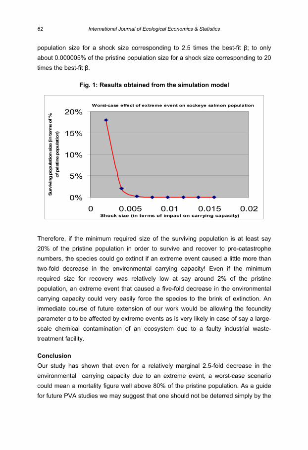
population size for a shock size corresponding to 2.5 times the best-fit ; to only

about 0.000005% of the pristine population size for a shock size corresponding to 20

times the best-fit .

Fig. 1: Results obtained from the simulation model

Therefore, if the minimum required size of the surviving population is at least say

20% of the pristine population in order to survive and recover to pre-catastrophe

numbers, the species could go extinct if an extreme event caused a little more than

two-fold decrease in the environmental carrying capacity! Even if the minimum

required size for recovery was relatively low at say around 2% of the pristine

population, an extreme event that caused a five-fold decrease in the environmental

carrying capacity could very easily force the species to the brink of extinction. An

immediate course of future extension of our work would be allowing the fecundity

parameter to be affected by extreme events as is very likely in case of say a large-

scale chemical contamination of an ecosystem due to a faulty industrial waste-

treatment facility.

Conclusion

Our study has shown that even for a relatively marginal 2.5-fold decrease in the

environmental carrying capacity due to an extreme event, a worst-case scenario

could mean a mortality figure well above 80% of the pristine population. As a guide

for future PVA studies we may suggest that one should not be deterred simply by the

Worst-case effect of extreme event on sockeye salmon population

0%

5%

10%

15%

20%

0 0.005 0.01 0.015 0.02Shock size (in terms of impact on carrying capacity)

Surv

ivin

g p

opula

tion s

ize (in

term

s o

f %

of pristine p

opula

tion)


notion that extreme events are uncontrollable and hence outside the purview of

computational modeling. Indeed the effect of an extreme event can almost always

prove to be fatal for a species but nevertheless, as our study shows, there is ample

scope and justification for future scientific enquiries into the relationship between

survival probability of a species and the adverse impact of an extreme event on

ecological sustainability.

References:

[1] Caswell, H. Matrix Population Models: Construction, Analysis and Interpretation.Sinauer Associates, Sunderland, MA, 2001.

[2] Hoppensteadt, F. C. Mathematical Methods of Population Biology. Cambridge Univ. Press, NY, 1982.

[3] Hoppensteadt F. C. and C. S. Peskin, Mathematics in Medicine and the Life Sciences. Springer-Verlag New York Inc., NY, 1992.

[4] Ricker, W. E. Stock and recruitment, J. Fish. Res. Bd. Canada 11, 559-623, 1954.

[5] N. Madras, Lectures on Monte Carlo Methods. Fields Institute Monographs, Amer. Math. Soc., Rhode Island, 2002.

[6] N. L. Johnson, S. Kotz and N. Balakrishnan, Continuous Univariate Probability Distributions, (Vol. 1). John Wiley & Sons Inc., NY, 1994.

[7] N. D. Wallace, Computer Generation of Gamma Variates with Non-integral Shape Parameters, Comm. ACM 17(12), 691-695, 1974.1

Acknowledgement: The authors are grateful to the anonymous referee for his/her insightful comments and suggestions

which went a long way in deciding the final shape of our paper.


Low-income Farmers’ Behavior toward Land Degradation: The Effects of Perceptions, Awareness, Attitude, and Land

Use

Budry Bayard1 , Curtis M. Jolly1*, Dennis A. Shannon2 and Alejandro A. Lazarte3

1Department of Agricultural Economics and Rural Sociology 2Department of Agronomy and Soils

3Department of Psychology Auburn University, Auburn, AL, USA

*Correspondence Author Department of Agricultural Economics and Rural Sociology

213 Comer Hall, Auburn University, AL 36849, USA Phone: 334-844-5613. Fax: 334-844-5639

E-mail: [email protected]

ABSTRACT

A structural equation modeling approach is used to examine the relationship between farmers’ perceptions of land degradation and their self-reported environmental behavior. Influence of crop dependency, land tenure, and demographic pressure on perceptions and behavior is also explored. Results showed that perceived susceptibility and severity of land degradation strongly influences farmers’ awareness of, and attitude toward environmental problems. Awareness of land resource depletion is likely to foster behavioral changes that will mitigate the problems. Greater financial and economic dependence on crop production causes greater perceived susceptibility, severity, benefits, and more positive attitude toward land degradation. Greater dependence on crops is associated with less perceived barriers to behavioral change. Direct ownership of the land is negatively related to perceived severity, and awareness, but positively associated with barriers and behavior.

Keywords: Structural; equation; perceptions; behavior; land degradation

JEL Classification: 62H, 62J


1. INTRODUCTION

With one of the fastest growing populations in the western world, Haitians

depend directly or indirectly on agriculture for their livelihood. Agricultural lands have

been under enormous pressure to produce food, fiber, and firewood for a growing


population (annual average growth rate of 1.67 percent [CIA World Fact Book,

2003]) for several decades. As the population increases, more and more marginal

lands are brought into production to satisfy market demand for food. The intensive

cultivation of those lands, most of which are unsuitable for agricultural production,

results in severe soil loss due to erosion, landslides, and finally a complete change

of landscape. This situation of declining soil fertility and loss of agricultural lands

keeps the Haitian economy in a chronic state of underdevelopment and exposure to

long-term climatic changes (Lundahl, 1996).

Farmers have partially responded to land resource depletion and the

concomitant declining agricultural productivity by adopting indigenous techniques,

such as contour trash barriers and contour bunds to retard the erosion process and

improve soil fertility (White and Jickling, 1995). In the face of farmers’ limited

capacity and laxity to reduce the land degradation problem, government and

international institutions have encouraged programs aimed at retarding the process

and improving the environment. Results of such programs have been less than

satisfying because of farmers’ reluctance to change their environmental attitude and

behavior.

Early studies (Saint-Dic, 1981) posit simplistic theories to explain farmers’ lack

of interest into changing behaviors and practices that may result in environmental

improvement. They point out farmers’ ignorance and conservatism in the face of

change. Other studies have been less critical, arguing that farmers’ environmental

attitude and behavior are related to the multiple constraints they face (Jean-Pierre,

1984; Murray, 1979). Recent studies (White and Quinn, 1992; Bayard, 2000;

Bannister, 2001) suggest that social, demographic, and economic factors are the

primary determinants of farmers’ environmental behavior.

Although several studies indicated that socio-economic factors may influence

farmers’ environmental behavior, little is understood about how their perceptions,

beliefs and attitude toward the environment may result in behavioral change. Even

more noticeable is that few attempts have been made to understand farmers’

perceptions and awareness of the environmental problem, and the underlying socio-

economic mechanism that may trigger the modification of poor farmers’ attitudes

toward the environment. Furthermore, analysis of the effect of farmers’ economic

and financial dependence on the land on their perceptions, attitude, and behavior


has not been conducted. This study investigates limited, resource Haitian farmers’

knowledge and perceptions of land degradation.

2. PREVIOUS RESEARCH

A number of studies worldwide have evaluated determinants of farmers’

environmental behavior. Some researchers (Gould et al., 1989; Bultena and

Hoiberg, 1983; Norris and Batie, 1987; Burton et al., 1999; Featherstone and

Goodwin, 1993) showed that socio-economic factors, including age and education,

significantly shape farmers’ environmental attitude and behavior. Financial factors,

such as short-term profitability and long-term asset value are important in explaining

farmers’ attitudes (McConnell, 1983; Barbier, 1990; Napier, 1991; Sain and Barreto,

1996).

Economic factors including farm income, off-farm revenue, and risk aversion

are found to influence soil conservation adoption decisions (Shields et al., 1993;

Lasley et al., 1990). Higher income is likely to increase adoption of land

management technologies (Lynne and Rola, 1988; Shields et al., 1993; Luzar and

Diagne, 1999) while off-farm activities may inhibit this decision (Lasley et al., 1990).

Institutional factors such as land tenure arrangements, membership in environmental

and local organizations, and technical assistance also play a significant role in

adoption of soil conservation techniques (Francis, 1986; Lee and Stewart, 1983;

Sureshwaran et al., 1996; Burton et al., 1999; Soule et al., 2000). Other studies

indicated that farm size, length and degree of slope, and soil erodibility are the

primary determinants of conservation behavior (Rahm and Huffman, 1984; Barbier,

1990; Huszar and Cochrane, 1990; Sureshwaran et al., 1996).

Results of the studies reported above were rather inconclusive and/or

conflicting. Studies by Ervin and Ervin (1982) and Rogers (1995) suggest that

perceptions and awareness of environmental problems are likely to influence

individuals’ behavior. According to those researchers, farmers perceive land

degradation problems before they decide whether to adopt or not to adopt a

conservation measure (Ervin and Ervin, 1982; Gould et al., 1989; Traoré et al., 1998;

Bultena and Hoiberg, 1983; Napier and Brown, 1993). They found farmers’ behavior

to be significantly related to their levels of perception of environmental problems.

Farm level studies, recognizing the importance of perceptions, emphasize

attitude as the prime determinant of environmental behavior. In the United States,


Lynne and Rola (1988), Luzar and Diagne (1999), and Bourke and Luloff (1994)

reported that farmers’ environmental attitude was significantly related to participation

in environmental programs.

In Europe, Willock et al. (1999a, 1999b), explored the correlations between

farmers’ attitude and objectives and environmental behaviors. Their results showed

significant positive correlations between environmentally oriented behaviors and

attitudes. Behaviors were also significantly correlated to farmers’ sustainability

objectives. Their results also indicated that attitudes and farmers’ goals have

significant positive correlations.

Pouta and Rekola (2001) found significant relationships between attitude and

behavioral intentions for abatement of forest regeneration in Finland. Attitudes are in

turn influenced by beliefs held about the outcomes of behavior. In Bangkok, Daniere

and Takahashi (1999) found that attitude and value variables are highly significant

predictors of environmental behavior. Other studies (Carr and Tait, 1991; Hines et

al., 1990; Kantola et al., 1982) observed significant correlations between attitude and

behavior. In one study, Kantola et al. (1982) found a positive effect of attitude and

social norms on intentions to conserve water. In another set of results, Kantola et al.

(1983) argued neither increasing severity of water pollution, nor efficacy influenced

farmers’ behavioral intentions in promoting water conservation.

In a study conducted in Austria, Vogel (1996) found that farmers’ behavior is

strongly related to their attitudes toward environmental problems in general, and

other issues related to their spheres of activity. In short, attitude may be a significant

determinant of environmental behavior. However, in some cases, attitude may be a

weak determinant of environmental behavior. In this study, the structure of farmers’

environmental attitude and behavior is analyzed, and the influence of the level of

economic dependence on crop production, land tenure, and demographic pressure

on farmers’ perceptions, awareness, attitude, and behavior toward land degradation

is also examined.

3. CONCEPTUAL FRAMEWORK

The theory of reasoned action (TRA) developed by Ajzen and Fishbein

(1977), and its extended version, the theory of planned behavior (TPB) (Ajzen and

Madden, 1986; Ajzen, 1991) connect attitude and behavior in a logical framework.

According to the TRA, intention is the most important determinant of action.


Behavioral intention refers to a person’s intention to perform various behaviors.

Intention in the TRA is specified as a function of attitude and subjective norms.

Attitude refers to the degree to which a person has a favorable or unfavorable

evaluation of an object. Attitude is influenced by a person’s beliefs that performing a

behavior will lead to a desired outcome.

In this study, we use the TRA framework and results from the empirical

studies reviewed above to examine the attitude-behavior relationship among low-

income farmers in Haiti. The study is based on the premise that farmers, who

primarily depend on the land for their livelihood, will develop an attachment to the

land and a strong concern for the environment, and perceive themselves as

environmentally responsible. However, the level of dependency on crop production

for their survival may complicate the development of a positive attitude toward the

environment. As indicated by Vogel (1996), farmers living in difficult conditions may

possess a higher perception of environmental problems. All categories of individuals

may be concerned about the degradation of the environment. Differences in

attitudes and behavior may result from different opportunities, constraints, and

perceptions.

The importance of the land in the Haitian context makes its improvement

desirable. To achieve a certain level of improvement in the environment, not only

are technological changes important, but also changes in attitudes and behaviors of

those involved in agriculture are necessary. Nevertheless, farmers’ beliefs may

enhance or inhibit confidence in their ability to perform a particular task.

We assess farmers’ perceptions of susceptibility, severity of land degradation,

benefits of environmental improvement, and social and technological barriers to

change. Influence of those psychological constructs on environmental awareness

and attitude is examined. Susceptibility refers to one’s perception of being affected

by environmental degradation. Perceived seriousness of land degradation is the

consciousness of the problem. Benefits refer to the perceived economic and social

benefits of environmental improvement; and barriers are the potential negative

consequences or factors that may hinder positive actions.

A structural model examining the nature of farmers’ environmental behavior is

developed in figure 1. Typically, the model postulates that perceived susceptibility to

land degradation, perceived seriousness of the problem, perceived benefit of

environmental improvement, and perceived barrier to behavioral change influence


farmers’ awareness of, and attitude toward environmental problems. Attitude and

awareness, in turn, affect self-reported behavior, suggesting a mediating role

between the perception factors and behavior. Finally, the model examines the effect

of crop dependency, land tenure, and demographic pressure on the perceptual

variables, awareness, attitude, and behavior. To determine the predictors of

farmers’ environmental behavior, we propose the following hypotheses:

Hypothesis 1: Farmers’ perceptions about environmental degradation will

influence their awareness of the problem and their attitude toward adopting

behaviors that will mitigate the problem.

Hypothesis 1a: The greater the perceived susceptibility to environmental

degradation, the more farmers become aware, and the more positive attitude they

will develop toward the environment.

Hypothesis 1b: The perception of seriousness of land degradation enhances

farmers’ level of awareness, and their attitude toward the environment.

Hypothesis 1c: The greater perception of physical, environmental, financial,

social, and economic benefits, the greater awareness, and the more positive attitude

will farmers have toward environmental improvement.

Hypothesis 1d: The greater the perception of barriers to actions towards

reducing environmental degradation, the weaker farmers’ awareness of and attitude

toward the environmental problem.

An important aspect of the study is the investigation of the relationship

between attitude and behavior. It is assumed that attitude is directly related to

behavior, and perceptions of land degradation, along with the level of dependence

on the land, will strengthen this relationship. Therefore, given the importance of the

land in all aspects of the farmer’s lives, we examine the following hypotheses:

Hypothesis 2: Farmers’ awareness of, and attitude toward the environment

will positively influence their behavior.

In the Haitian peasant economy, land is an important factor as most Haitians

are culturally tied to this natural resource, and economically and financially

dependent on it for their survival.

Hypothesis 3a: Farmers’ economic and financial dependency on crop

production positively influences their perceptions of the susceptibility, seriousness of

environmental degradation, and perceived benefits of environmental improvement,

and negatively influences their perception of the barriers to behavioral change.


Hypothesis 3b: Farmers’ economic and financial dependency on crops

positively influences their awareness of land degradation, and their attitudes and

behavior toward the problem.

Hypothesis 3c: Farmers who directly own the land they operate are less likely to be

concerned about environmental degradation, but more likely to change their behavior

toward the problem.

4. METHOD

4.1. Study area

The study was conducted in two regions in Haiti: the South and the

Southeast. These regions were selected because of the observed levels of land

degradation, because of farmers’ exposure to soil and water conservation projects,

and previous participation by villagers in soil management practices that are likely to

raise their awareness of the problems. In the South, field surveys were conducted in

Gaita and Bannate, two villages within the community of Camp-Perrin, where

farmers have been exposed to soil conservation projects conducted by development

agencies in collaboration with local organizations.

Cultivated lands in the area of Gaita and Bannate are on elevations of 100 to

300 meters above sea level. The average annual rainfall is usually between 1,500

and 2,000 millimeters. Rainfall in the region, occurring from February to November,

is highly variable with a bimodal seasonal distribution. The first rainy season lasts

from February to May, and the second from July to November. This regional rainfall

distribution pattern allows two planting seasons per year.

In the Southeastern region, data were collected in three locations including

Cap-Rouge, Cayes-Jacmel, and Marigot. For the last three decades, several

development projects conducted activities related to coffee production, planting and

grafting of fruit trees, and diffusion of other soil management practices (Macroscope,

1997). The research site in this region varies in elevation from 200 to 500 meters.

The average annual rainfall in this region varies from 1,000 to 1,500 millimeters.

In both regions, the farming systems are characterized by the production of

various annual crops. The major food crops, which include corn, sorghum, beans,

cassava, yams, and sweet potato, occupied steeply sloping lands that are classified

as more appropriate for forest uses. The slopes of cultivated plots in the regions can

be more than 60 percent. Some farmers produce perennial crops, such as coffee


and cocoa, that provide them with substantial cash earnings. Hillside farming in

these regions is especially intensive. The farming system is dominated by a rotation

of maize/beans and maize/sorghum/pigeon peas with minimal levels of purchased

inputs and intensive use of family labor. Both regions suffer severe soil erosion

problems due to the agro-climatic conditions on one hand, and the lack of soil

protection on the other. Coupled with a short fallow period of one to two years, the

degradation of the soil causes the decline of the fertility level, and consequently

reduces crop yields. For several decades, the Haitian government and development

agencies have promoted soil conservation projects in an attempt to reduce land

degradation. Nevertheless, farmers have failed to extensively adopt the techniques

promoted which include rock walls, contour canal, and hedgerows.

Unlike many basically subsistence-oriented farmers, agricultural producers in

the study areas are highly integrated into a market economy. While the farmers’

primary goal is food self-sufficiency, a large proportion of agricultural surplus is sold

on the market. Production and market risks often threaten the farmers’ well being,

and force them to develop survival strategies, including agricultural diversification,

off-farm activities, and selective migration.

4.2. Data collection

Interviews with farmers in both regions were carried out in two successive

phases. In the first phase, a random sample of 240 farm operators from the

Southern area, and 360 from the Southeastern region was taken, and data were

collected through personal interviews between July and August 2000. A second set

of interviews was carried out between January and March 2002 to collect additional

information not included in the previous survey. Upon completion of the field survey,

six interviews were discarded for incomplete information. Thus, 594 observations

remained for the final analysis, constituting 99 percent usable questionnaires.

4.3. Survey instrument

Two survey instruments were developed for the purpose of the interviews.

The first questionnaire which was used in the first phase gathered information on

farm structure and operators’ characteristics. Information was also collected on

farmers’ awareness of, and attitude toward soil erosion and land degradation, their

perception of susceptibility, their appraised severity of environmental degradation,


the benefits of conservation and the perceived barriers to change. The survey

instrument used in the second phase gathered information on farmers’ goals,

opinions on policy formation, and environmental behavior. Questions related to

perceptions, awareness, attitude and behavior were measured on a five-point scale

in terms of how strongly the respondents felt about a set of statements. The

responses were weighted 1 to 5 with lower values indicating greater agreement (see

Bayard, 2003 for more details). Prior to the field survey, pretests of the

questionnaires were conducted with a group of farmers in both regions.

4.4. Variable measurement and model estimation

The variables representing perceived susceptibility, perceived severity,

benefits, barriers, awareness and attitude were recorded by asking farmers to scale

a set of questions that expressed their beliefs about each issue. These questions

evaluated farmers’ attitudes toward ecological, social, and economic problems

related to environmental degradation. Behavior was recorded by asking farmers a

set of questions that indicated actions they have taken, or intend to take to improve

the environment.

Exploratory factor analyses were conducted on the data to extract the items

that measure each construct using the SAS software system (Hatcher, 1994). Each

set of items defining a particular construct was submitted separately to factor

analysis. The scree test was used to determine the number of meaningful factors

retained for interpretation, and an orthogonal varimax rotation was used. A reliability

assessment (Cronbach’s alpha) was used to check for internal consistency of each

factor.

Structural equation modeling was used to test the hypotheses developed in

the study using Maximum Likelihood Estimation procedures. We used a system of

simultaneous equations to accommodate the structural model developed in Figure 1.

Equations 1 and 2 depict relationships between observed indicators and latent

variables for exogenous and endogenous variables, respectively.

x = x + (1)

y = y + (2)


where x and y are the q × 1 and p × 1 vectors of observed variables; x is the q × m

matrix of regression coefficients of x on ; y is the p × m matrix of coefficients of the

regression of y on ; is the n × 1 matrix of random vector of the latent exogenous

variables representing perceived susceptibility ( 1), perceived seriousness ( 2),

perceived benefits ( 3), and perceived barriers ( 4); is the m × 1 matrix of random

vector of latent endogenous variables representing awareness ( 1), attitude ( 2), and

behavior ( 3); and and are q × 1 and p × 1 vectors of measurement errors in x

and y, respectively. The following equations were used to estimate the hypothesized

causal relationships:

1 = 11 1 + 12 2 + 13 3 + 14 4 + 15CD + 16LT + 17DP + 1 (3)

2 = 21 1 + 22 2 + 23 3 + 24 4 + 25CD + 26 LT + 27DP + 2 (4)

3 = 31 1 + 32 2 + 33CD + 34LT + 35DP + 3 (5)

1 = 11CD + 12LT + 13DP + 4 (6)

2 = 21CD + 22LT + 23DP + 5 (7)

3 = 31CD + 32LT + 33DP + 6 (8)

4 = 41CD + 42LT + 43DP + 7 (9)

where CD, LT, and DP are manifest exogenous variables representing crop

dependency, land tenure, and demographic pressure, respectively; is the m × m

matrix of coefficients relating the latent endogenous variables, is the m × n matrix

of the -variables in the structural relationship between and , and is the

coefficient for the effects of land dependency on . It is assumed that E( ) = 0, E(

�) = 0, E( �) = . Crop dependency is calculated as the share of crop earnings

in total household income. Land tenure represents an index of the ration of the size

of land directly owned by farm size. Demographic pressure is measured as the

number of people dependent on the household divided by the size of the farm. The

analyses were conducted using Lisrel 8.54 (du Toit and du Toit, 2001; Jöreskog and

Sörbom, 2001). In the line of Anderson and Gerbing’s (1988) two-stage approach,

the measurement model was first evaluated, then, the structural paths were

estimated. Model fit was assessed using the normed-fit and goodness-of-fit indices,

as well as the comparative fit index.


5. EMPIRICAL RESULTS

5.1. Demographic profile of the respondents

Of the 594 respondents, male farmers made up 85 percent of the total

sample, whereas females represented 15 percent. The average age of surveyed

farmers was 48 years, ranging from 22 to 86 years. Approximately half of the

respondents were between 35 and 50 years of age.

The survey reveals that 63 percent of the respondents had some primary

school level of education. Thirty-two percent had no formal education, and only 5

percent of the respondents had continued their studies beyond primary level. Fifty-

nine percent of surveyed farmers declared that they pursued some type of

educational training in soil conservation. Sixty-seven percent of the farmers

interviewed are members of local groups, while 33 percent do not belong to any local

organizations. Twenty-one percent of those who belong to a group had assumed, at

one time or the other, a leadership position.

The average size of households in the study areas is 6.33 ranging from one to

18 individuals. Given the small size of plots operated by farmers, the average

density of a farm household is about seven people per hectare (ha). Forty-seven

percent of the farm households had a population density of less than five people.

Households with five to 10 and more than 10 people per hectare made up 35 percent

and 18 percent of the sample, respectively. These reveal that a relatively high level

of pressure is being exerted on household resources in these regions.

5.2. Farm structure

The typical Haitian farm enterprise is composed of numerous plots for which

land tenure arrangements vary. The various plots that a farm household may

manage are often located in different agro-ecological areas, allowing farmers to grow

a variety of crops including cereals, vegetables, and fruits. This land distribution

pattern allows farmers to spread food availability over the entire year; therefore,

limiting the risk of starvation.

Farmers in the study areas cultivate an average of 5.23 plots ranging from

one to 18. The majority of the farms (52 percent) are composed of five to 10 plots.

Despite the relatively large number of plots cultivated, the size of a farm in the study

areas is small averaging 1.48 hectares. Forty-seven percent of the farms are


between one and three ha. The plots are cultivated under various land tenure

arrangements including purchase, inheritance, share-cropping, renting, and

temporary use of family plots. Nevertheless, direct ownership via purchase is the

most important source of access to land in the research sites. Direct ownership

represents 56 percent of all cultivated land in the research areas.

Farm household income is generated from a multitude of activities in which

family members are involved. Agriculture is the primary source of earnings for the

numerous people in the study areas. However, household members are involved in

a number of off-farm activities, including forest exploitation, petty trade, and off-farm

jobs that bring additional income in the household on a regular basis. The estimated

per capita income per year for a household is on average 1,871 gourdes (1gourde =

U.S.$ 0.05) ranging from 19 to 15,790 gourdes. Most farmers (61 percent) have an

annual per capita income of over 1,000 gourdes. Revenues from selling crops

grown on the farm represent 74 percent of the household earnings. Share of animal

production represents 18 percent, whereas off-farm earnings make up 8 percent of

total family income. Although farmers are involved in a multitude of economic

activities that bring revenue to the household, they are highly dependent on the land

for their survival.

5.3. Farmers’ perceptions of environmental problems

Numerous indicators were used to assess farmers’ perceptions of

environmental problems. The indicators describe their susceptibility towards, and

their perceived severity of the degradation of the environment, their perceived

benefits of environmental improvement, and the self-imposed barriers that may

hinder actions to improve the environment. Table 1 shows the factor analysis results

for the items defining the perception factors.

Perceived susceptibility suggests that respondents do not perceive

themselves as being affected by erosion problems because they have taken

conservation measures to prevent them. Four items, with loading greater than 0.40,

were retained. Cronbach’s alpha coefficient for the susceptibility factor was 0.80

indicating a relatively good internal consistency. The seriousness of the problem

shows how land degradation may affect the farmer, the community, and country’s

welfare. In terms of perceived seriousness of environmental problems, five items

with loadings greater than 0.40 were retained by the factor analysis. The items


mainly reflect the perception of the damages caused by erosion at the farm level.

The reliability coefficient for this factor is estimated at 0.83.

Five indicators define farmers’ perceived benefits of environmental

improvements (Table 1). The items reflect farmers’ decisions to adopt conservation

measures that are in themselves beneficial and can improve the land because they

result in positive outcomes. Reliability coefficient for the benefit factor was 0.89.

Factor analysis suggests seven items that measure perceived barriers to

environmental improvement. The items deal with various types of issues including

social and physical barriers. These items have high loadings on the perceived

barrier factor. The coefficient alpha for barrier factor was 0.84 suggesting that the

scale measuring the items is reliable.

5.4. Farmers’ environmental awareness, attitude, and behavior

Awareness of land degradation is an important step toward undertaking

remedial actions. Farmers must be aware of erosion problems, of their

consequences, and measures that halt environmental degradation before they can

engage in any conservation behavior. Awareness of the problem should generate

greater willingness to change agricultural practices that will engender environmental

improvement. To assess farmers’ awareness of environmental degradation in Haiti,

farmers were asked to indicate their agreement with the knowledge of various

environmental issues. Table 2 shows the items used to define the awareness factor.

Seven items, with loadings greater than 0.40, define the awareness factor.

The scales of these variables demonstrate a high level of reliability with an estimate

of 0.78. Items that load heavily on the awareness factor cover a wide range of

issues. The items of the awareness factor are related to knowledge of the existence

of erosion problems at the national, local, and farm levels. Two of the variables

capture the impact of erosion on soil nutrients and crop yields. The two final items

demonstrate the effect of farming practices and tree cutting on the process of

erosion. It appears from these results that items directly related to activities on the

farm have the highest loadings on the awareness factor.

The items dealing with farmers’ environmental attitudes reflect the global

effects of soil erosion and the individuals’ responsibility in the process. The

attitudinal factor consists of seven items with loadings greater than 0.40. The


attitudinal factor seems to have a relatively good reliability with an alpha coefficient

of 0.83.

To assess individuals’ environmental behavior, a number of statements were

included in the questionnaire that elicited the reasons why farmers adopted

measures to retard environmental degradation. Table 2 reports the selected items

that load on the behavioral construct. All the items, but two had loadings greater

than 0.70. The behavior factor had a coefficient of reliability of 0.72, indicating a

reasonable internal consistency.

5.5. Determinants of environmental perceptions, awareness, attitude, and behavior

We used a structural model in Lisrel (Jöreskog and Sörbom, 2001) to examine

the determinants of the structure of farmers’ environmental behavior. The maximum

likelihood estimation results are reported in Table 3. Chi-square statistics is often

used to assess the fit of structural equation models. However, sample sizes tend to

inflate this statistic (Vaske and Kobrin, 2001; Byrne, 1998). Consequently, it is

suggested that the chi-square should be evaluated in relation to the model’s degree

of freedom (Marsh and Hocevar, 1985; Vaske and Kobrin, 2001; Jöreskog and

Sörbom, 2001). A 2/df ratio along with other indicators, such as the Normed Fit

Index (NFI), the Goodness of Fit Index (GFI), and Root Mean Square Error

Approximation (RMSEA) are suggested as measures of fit. A 2/df ratio between 2:1

and 5:1 indicates an acceptable fit (Marsh and Hocevar, 1985). Byrne (1998) and

Bentler (1990) also suggested the use of the Comparative Fit Index (CFI) to assess

the fit of a structural model. A value of 0.90 and above for NFI, CFI, and GFI is

considered good fit.

The overall fit of the model was assessed using the NFI, GFI, and CFI.

Values for NFI, GFI, and CFI were 0.95, 0.92, and 0.96, respectively. Hence, the

indices suggest that the overall fit of the model is acceptable.

Among the perceptual factors, perceived susceptibility and severity of

environmental degradation were found to influence farmers’ awareness of the

problem. The standardized path coefficients for perceived susceptibility and severity

factors are 0.24 (t= 2.36) and 0.35 (t=5.24), respectively. The coefficients were

significant at 5 percent level supporting the hypotheses that perceived susceptibility

and severity of environmental degradation were positively related to awareness.

This result is interesting in the sense that soil erosion is a widespread phenomenon


throughout Haiti. Several indicators dealing with the effects of land degradation on

the agricultural production process define the severity factor. The degradation of the

environment impacts individuals’ lives at different levels. Farmers on the hillside

continuously observe the physical aspect of the erosion process and experience its

effects on agricultural production. Given their direct experience with the problem,

farmers have developed a good understanding of the negative effects of erosion on

soil nutrients, crop yields, and of other environmental damages. Therefore, the more

severe they perceived the damage and the more susceptible they feel about it, the

more they become aware of the extent of environmental degradation in Haiti. It is

evident that the impact of soil erosion would be greater in the more eroded areas

than it is in less eroded ones. Hence, farmers in the most affected areas may be

more aware of erosion problems than those in less eroded areas.

Results of the model also support the hypotheses that perceived susceptibility

and perceived severity influence farmers’ attitude toward the environment. The

perception of susceptibility was positively related to attitude toward the environment.

As shown in Table 3, the standardized coefficient for the susceptibility factor was

0.44 (t = 4.65), suggesting a significant influence on attitude. The results suggest

that farmers who feel susceptible to land degradation are more likely to develop a

positive attitude toward the environment. The perceived severity factor was

positively related to the attitude variable. The standardized path coefficient for this

variable was 0.22, with a t-value of 4.18. Increasing perceived severity of

environmental degradation tends to promote a positive attitude of Haitian farmers

toward the environment.

Results of the model show that awareness of environmental degradation has

a significant causal effect on farmers’ environmental behavior. As hypothesized,

greater awareness of the degradation of the environment leads farmers to take

measures to reduce the problem. The standardized coefficient of awareness on

behavior is 0.30 (t = 4.32). It appears that perceived susceptibility and severity of the

degradation of the environment are the most important factors influencing a change

of environmental behavior. The influence of these variables on behavior is mediated

by the awareness factor.

One of the hypotheses in this study is that farmers’ dependence on the land

for crop production will have a significant effect on their perceptions, awareness,

attitude, and behavior. As mentioned earlier in this study, Haitian farmers depend


heavily on the land for their survival. Not only that the staples produced are primarily

used for home consumption, but also, a fraction of the production is sold on the

market, allowing farmers to participate in commercial transactions. The results

support the hypothesis that crop dependency influences farmers’ perceptions of

environmental problems. Dependency on crop production significantly affects

perceptions of susceptibility, severity of land depletion, benefit of and barriers to

environmental improvement. The coefficients of crop dependency on susceptibility,

severity, benefit, and barriers are 0.36 (t = 8.25), 0.20 (t= 4.32), 0.30 (t= 6.97), and -

0.16 (t=-3.61), respectively. Attitude toward environmental degradation is also

affected by the level of economic and financial dependence on crops produced. The

results show that attitude toward land degradation increases with the level of

dependence on crops. The standardized coefficient of land dependency on attitude

is 0.10 (t = 2.32). This result supports the hypothesis that greater dependence on

crop engenders a more positive attitude toward environmental problems among

farmers. In general, Haitians living in rural areas depend on the land for their

survival. Some farmers have off-farm jobs that compete with farming activities.

Others have no other alternative than farming. Therefore, their only means to make

a living is to keep exploiting the limited land they operate.

Land tenure arrangements are often considered important factors in land

management decisions. Results of this study show that ownership of the land is

negatively related to awareness of environmental degradation ( 16= -0.13), and

perceived severity of the problems ( 22= -0.13), but positively associated with

barriers ( 32=0.12) and behavior ( 34= 0.09).

6. DISCUSSIONS AND CONCLUSIONS

This study focuses on the influence of perceptual variables on low-income

farmers’ awareness of environmental degradation, their attitude and behavior toward

the problem, and the role played by land use in shaping their perceptions. The

present results suggest that Haitian farmers are aware of the degradation of the

environment in their country. Their strong agreement with statements underlying

awareness showed that their understanding and knowledge of the problem are lucid.

An important finding of this research is the effect of farmers’ perceived

severity of land degradation on their awareness. Results of this research also show

that perception of the severity of land degradation is influential in determining


farmers’ attitude toward the environment. Perception of the severity of

environmental degradation appears to play a significant role in raising farmers’

awareness and shaping their attitude. This result appears to corroborate findings

from previous research (Gould et al., 1989, Bultena and Hoiberg, 1983). Land

degradation affects people’s lives at various levels. Farmers who are dealing with

this problem on a daily basis may have observed the phenomenon of land

degradation on their farms and surrounding areas. In fact, the items defining the

perceived severity of land degradation deal with issues directly related to farmers’

well-being. They include the physical damage caused by erosion on plots, the

negative impacts of erosion on soil nutrients and crop yields, and the threat to food

security. All these issues denote farmers’ evaluations of the impacts that land

degradation may have on their ability to produce food for their family and to generate

income for their welfare. Hence, greater perceptions of the severity of land

degradation will cause greater awareness, and ultimately a greater inclination to

embrace change.

Beside perceived severity of environmental damage, farmers’ awareness of

and attitude toward the environment was greatly affected by their perceived

susceptibility to the problem. These results suggest that farmers will be more aware

and inclined to develop a positive attitude toward environmental sustainability if they

feel directly exposed to the problem. As indicated by Leventhal et al. (1965),

individuals facing a particular threat consider their susceptibility to, and the severity

of the problem. Immediate threats of soil erosion, for instance, will cause a more

positive attitude toward the environment. The implication of these findings is that

policy makers need to develop strategies to point out the importance of the

seriousness of land degradation to the farming population. Not only is it important to

stress the extensiveness of environmental damage, but also the consequences of

not taking appropriate and immediate actions.

An important question raised is the extent to which farmers’ attitude and

awareness influence their behavior. Findings of this research support the hypothesis

that awareness of environmental degradation significantly influences behavior.

According to this result, supported by Napier and Napier (1991), greater awareness

of environmental degradation is likely to cause farmers to change their behavior.

This finding elucidates the mediating role of awareness in explaining the


relationships between farmers’ perception of the susceptibility to and severity of land

degradation and their environmental behavior.

A critical finding of this research is the influence of crop dependency on the

perceptual variables, and farmers’ environmental attitude. Dependence on crop

production directly influences farmers’ perceived susceptibility, severity, benefits,

barriers, and attitude toward environmental problems. These findings suggest that

decisions should be made to improve agricultural production in order to increase

earnings from that sector. Particular attention should be given to individuals who

show great attachment to the land.

Another issue addressed in the study is the importance of land tenure in

shaping individual’s perceptions of land degradation. It appears that farmers who

have more security on the land they operate are less aware of environmental

damage, perceive the problem less severe, and impose greater barriers to change

than those who have little control over their land. However, individuals who directly

control their land are more likely to change their behavior. This situation is typical in

areas where soil management projects are implemented. Farmers who own their

land seem to be indifferent to land degradation because they are often economically

well-off. They are ready to embrace change in order to obtain benefits from project

interventions. It is apparent from the paths coefficients that dependency on crops

has a stronger effect on their perceptions than does land tenure.

This study represents an attempt to develop a structural model to explain low-

income farmers’ environmental behavior. The causal effects of psychological and

socio-economic factors on farmers’ environmental behavior were evaluated. The

study provides some useful insights on the determinants of farmers’ environmental

behavior structures, but it has one caveat. The nature of the statements and

questions and farmers’ levels of understanding may have increased respondents’

biases. However, particular attention was paid in the design of the survey instrument

and during training sessions to reducing enumerator’s bias. Nevertheless, this study

makes a significant contribution to the stock of knowledge of resource poor farmers’

environmental behavior. The information generated in the study is particularly useful

in addressing policy issues in terms of resource allocation to programs aimed at

coping with behavior modification to reduce environmental degradation in Haiti.


REFERENCES

Ajzen, I., 1991, The Theory of Planned Behavior, Organizational Behavior and Human Decision Process, 50, 179-211.

Ajzen, I., and Fishbein. M. 1977, Attitude-Behavior Relations: A Theoretical Analysis and Review of Empirical Research, Psychological Bulletin, 34 (5), 888-918.

Ajzen, I., and Madden. T.J. 1986, Prediction of Goal Directed Behavior: Attitudes, Intentions, and Perceived Behavioral Control, Journal of Experimental Social Psychology, 22, 453-474.

Anderson, J.C., and Gerbing. D.W. 1988, Structural Equation Modeling in Practices: A Review and Recommended Two-step Approach. Psychological Bulletin, 103 (3), 411-423.

Bannister, M.E., 2001, Dynamics of Farmer Adoption, Adaptation, and Management of Soil Conservation Hedgerows in Haiti, Doctoral Dissertation, University of Florida, Gainesville, Florida.

Barbier, E.B., 1990, The Farm-level Economics of Soil Conservation: The Uplands of Java, Land Economics, 66 (Feb.), 199-211.

Bayard, B., 2000, Adoption and Management of Soil Conservation Practices in Haiti: The Case of Alley Cropping and Rock Walls, Master Thesis, Auburn University, Auburn, Alabama.

Bayard, B., 2003, Environmental Self-efficacy and Behavior of Limited Resource Farmers in Haiti, Doctoral Dissertation, Auburn University, Auburn, Alabama.

Bentler, P.M., 1990, Comparative Fit Indexes in Structural Models, Psychological Bulletin, 107 ( 2), 238-246.

Bourke, L., and Luloff. A.E. 1994, Attitudes toward the Management of Nonindustrial Private Forest Land, Society and Natural Resources, 7, 445-457.

Bultena, G.L., and Hoiberg. E.O. 1983, Factors Affecting Farmers’ Adoption of Conservation Tillage, Journal of Soil and Water Conservation, 38 (May-June), 281-284.

Burton, M., Rigby, D., and Young. T. 1999, Analysis of the Determinants of Adoption of Organic Horticultural Techniques in the UK, Journal of Agricultural Economics, 50(1), 47-63.

Byrne, B.M., 1998, Structural Equation Modeling with LISREL, PRELIS, and SIMPL: Basic Concepts, Applications, and Programming, Lawrence Erlbaum Associates, Publishers, Mahwah, New Jersey.

Carr, S., and Tait. J. 1991, Differences in the Attitudes of Farmers and Conservationists and their Implications, Journal of Environmental Management,32, 281-294.

CIA (Central Intelligence Agency), 2003, The World Factbook (Haiti). Available from www.cia.gov/cia/publications/factbook/geos/ha.html.


Daniere, A.G., and Takahashi. L.M. 1999, Environmental Behavior in Bangkok, Thailand: A Portrait of Attitudes, Values, and Behavior, Economic Development and Cultural Change, 47 (3), 525-557.

du Toit, M., du Toit. S. 2001, Interactive Lisrel: User’s Guide, Scientific Software International, Lincoln, Illinois.

Ervin, C.A., and Ervin. D.E. 1982, Factors Affecting the Use of Soil Conservation Practices: Hypotheses, Evidence, and Policy Implications, Land Economics, 58 (3), 277-291.

Featherstone, A.M., and Goodwin. B.K. 1993, Factors Influencing a Farmers’ Decision to Invest in Long-term Conservation Improvements, Land Economics, 69(1), 67-81.

Francis, P.A. 1986, Land Tenure System and the Adoption of Alley Farming. inKang, B.T., Reynolds, L. (Ed.) Alley Farming in the Humid and Subhumid Tropics, Proceedings of International Workshop Held at Ibadan, Nigeria, March10-14, 182-195.

Gould, B.W., Saupe, W.E., and Klemme. R.M. 1989, Conservation tillage: The Role of Farm and Operator Characteristics and the Perception of Soil Erosion, Land Economics, 65 (2), 167-182.

Hatcher, L., 1994, A Step-by-Step Approach to Using the SAS System for Factor Analysis and Structural Equation Modeling, SAS Institute, Cary, NC.

Hines, J.M., Hungerford, H.R., and Tomera. A.N. 1990, Analysis and Synthesis of Research on Responsible Environmental Behavior: A Meta-Analysis, Journal of Environmental Education, 21 (4), 20-26.

Huszar, P., and Cochrane. H.C. 1990, Constraint to Conservation Farming in Java’s Uplands, Journal of Soil and Water Conservation, 45 (May-June), 420-423.

Jean-Pierre, J.D., 1984, L’aménagement de Bassins Versants Face aux Contraintes Economiques Paysannes: Une Analyse Empirique de la Problématique de la Lutte Anti-érosive en Haïti, Master Thesis, Université Laval, Québec.

Jöreskog, K., and Sörbom. D. 2001, LISREL 8: User’s Reference Guide, Scientific Software International, Lincoln, Illinois.

Kantola, S.J., Syme, G.J, and Campbell. N.A. 1982, The Role of Individual Differences and External Variables in a Test of Sufficiency of Fishbein’s Model to Explain Behavioral Intentions to Conserve Water, Journal of Applied Social Psychology, 12 (1), 70-83.

Kantola, S.J., Syme, G.J., and Nesdale. A.R. 1983, The Effects of Appraised Severity and Efficacy in Promoting Water Conservation: An Informational Analysis,Journal of Applied Social Psychology, 13 (2), 164-182.

Lasley, P., Duffy, M., Kettner, K., and Chase. C. 1990, Factors Affecting Farmers’ Use of Practices to Reduce Commercial Fertilizers and Pesticides, Journal of Soil and Water Conservation, 45 (Jan.-Feb.), 132-136.

Lee, L., and Stewart. W. 1983, Land Ownership and the Adoption of Minimum Tillage, American Journal of Agricultural Economics, 65, 256-64.


Leventhal, H., Singer, R.P., and Jones. S. 1965, The Effect of Fear and Specificity of Recommendations on Attitude and Behavior, Journal of Personality and Social Psychology, 2, 20-29.

Lundahl, M., 1996, Income and Land Distribution in Haiti: Some Remarks on Available Statistics, Journal of Interamerican Studies and World Affaires, 38, 109-126.

Luzar, E. J., and Diagne. A. 1999, Participation in the Next Generation of Agriculture Conservation Programs: The Role of Environmental Attitudes, Journal of Socio-Economics, 28, 335-349.

Lynne, G.D., and Rola. L.R. 1988, Improving Attitude-Behavior Prediction Models with Economic Variables: Farmer Actions Toward Soil Conservation, The Journal of Social Psychology, 128 (1), 19-28.

Lynne, G.D., Shonkwiler, J.S., Rola. L.R. 1988, Attitudes and Farmer Conservation Behavior, American Journal of Agricultural Economics, (Feb), 12-19.

Macroscope, 1997, Coopératives, une Voie pour le Développement Agricole en Haïti, Etude réalisée pour le compte de la Société de Coopération pour le Développement International. Port-au-Prince, Haïti.

Marsh, H.W., and Hocevar. D. 1985, Application of Confirmatory Factor Analysis to the Study of Self-concept: First and Higher Order Factor Models and their Invariance Across Groups, Psychological Bulletin, 97, 562-582.

McConnel, K.E., 1983, An Economic Analysis of Soil Conservation, American Journal of Agricultural Economics, 65 (Feb.), 83-9.

Murray, G.F., 1979, Terraces, Trees and the Haitian Peasant: An Assessment of Twenty-five Years of Erosion Control in Rural Haiti,USAID/Port-au-Prince, Haiti.

Napier, T.L., 1991, Factors Affecting Acceptance and Continued Use of Soil Conservation Practices in Developing Societies: A Diffusion Perspective, Agriculture, Ecosystems and Environment, 36, 127-140.

Napier, T.L., and Brown. D.E. 1993, Factors Affecting Attitudes Toward Groundwater Pollution Among Ohio Farmers, Journal of Soil and Water Conservation, 48 (5),432-438.

Napier, T.L., and Napier. A.S. 1991, Perceptions of Conservation Compliance Among Farmers in a Highly Erodible Area of Ohio, Journal of Soil and Water Conservation, 46 (3), 220-24.

Norris, P.E., and Batie. S.S. 1987, Virginia Aarmers’ Soil Conservation Decisions: An Application of Tobit Analysis, Southern Journal of Agricultural Economics, 19 (1), 79-90.

Pouta, E., and Rekola. M. 2001, The Theory of Planned Behavior in Predicting Willingness to Pay for Abatement of Forest Regeneration, Society and Natural Resources, 14 (2), 93-106.

Rahm, M.R., and Huffman. W.E. 1984, The Adoption of Reduced Tillage: The Role of Human Capital and Other Variables, American Journal of Agricultural Economics, (Nov.), 405-413.


Rogers, E.M., 1995, Diffusion of Innovations, Fourth edition, New York, the Free Press.

Sain, G.E., and Barreto. H.J. 1996, The Adoption of Soil Conservation Technology in El Salvador: Linking Productivity and Conservation, Journal of Soil and Water Conservation, 51 (April), 313-321.

Saint-Dic, R., 1981, Syst�me de Tenure et Lutte Anti-érosive en Haiti, Master thesis, Université Laval, Québec.

Shields, M.L., Rayuniyar, G.P, and Goode. F.M. 1993, A Longitudinal Analysis of Factors Influencing Increased Technology Adoption in Swaziland, 1985-1991, The Journal of Developing Areas, 27 (July), 469-484.

Soule, M.J., Tegene, A., and Wiebe. K.D. 2000, Land Tenure and the Adoption of Conservation Practices, American Journal of Agricultural Economics, 82 (4), 993-1005.

Sureshwaran, S., Londhe, S.R., and Frazier. P. 1996, A Logit Model for Evaluating Farmer Participation in Soil Conservation Programs: Sloping Agricultural Land Technology on Upland Farms in the Philippines, Journal of Sustainable Agriculture, 7 (4), 57-69.

Traoré, N., Landry, R., and Amara. N. 1998, On-Farm Adoption of Conservation Practices:

The Role of Farm and Farmer Characteristics, Perceptions, and Health Hazards,Land Economics, 74 (1), 114-27.

Vaske, J.J., and Kobrin. K.C. 2001, Place Attachment and Environmentally Responsible

Behavior, Journal of Environmental Education, 32 (4), 16-21.

Vogel, S., 1996, Farmers’ Environmental Attitudes and Behavior: A Case Study for Austria, Environment and Behavior, 28 (5), 591-613.

White, T.A., and Jickling. J.L. 1995. Peasants, Experts, and Land Use in Haiti: Lessons from Indigenous and Project Technology, Journal of Soil and Water Conservation, 50 (1), 7-14.

White, T.A., and Quinn. R.M. 1992, An Economic Evaluation of the Maissade, Haiti, Integrated Watershed Management Project, EPAT/MUCIA Working Paper, No. 2.

Willock, J., Deary, I.J., Edwards-Jones, G., Gibson, G.J., McGregor, M.J., Sutherland, A., Dent, J.B., Morgan, O., and Grieve. R. 1999a, The role of Attitudes and Objectives in Farmer Decision Making: Business and Environmental-Oriented Behavior in Scotland, Journal of Agricultural Economics, 50 (2), 286-303.

Willock, J., Deary, I.J., McGregor, M.J., Sutherland, A., Edwards-Jones, G., Morgan, O., Dent, J.B., Grieve, R., Gibson, G.J., and Austin. E. 1999b, Farmers’ Attitudes, Objectives, Behaviors, and Personality Traits: The Edinburgh Study of Decision Making on Farms, Journal of Vocational Behavior, 54, 5-36.


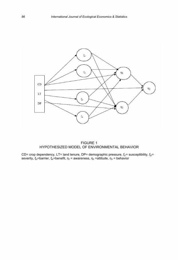
FIGURE 1 HYPOTHESIZED MODEL OF ENVIRONMENTAL BEHAVIOR

CD= crop dependency, LT= land tenure, DP= demographic pressure, 1= susceptibility, 2=severity, 3=barrier, 4=benefit, 1 = awareness, 2 =attitude, 3 = behavior


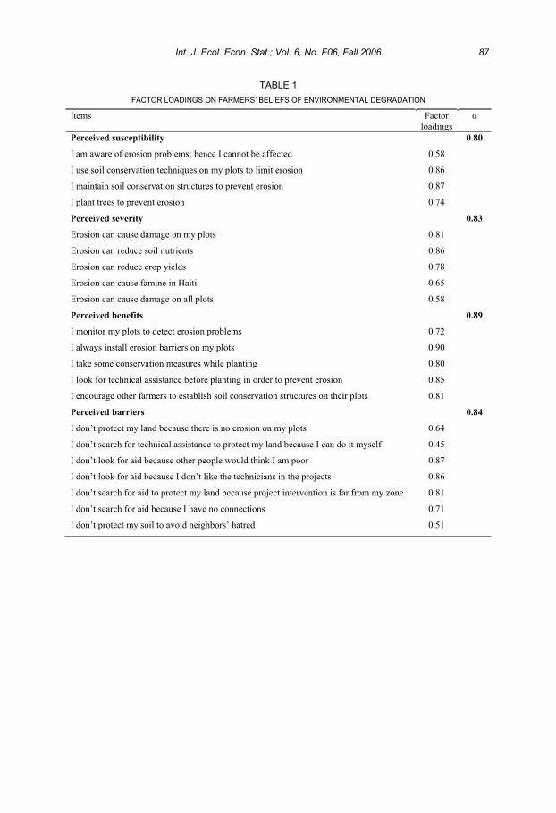
TABLE 1

FACTOR LOADINGS ON FARMERS’ BELIEFS OF ENVIRONMENTAL DEGRADATION

Items Factor

loadings

Perceived susceptibility

I am aware of erosion problems; hence I cannot be affected

I use soil conservation techniques on my plots to limit erosion

I maintain soil conservation structures to prevent erosion

I plant trees to prevent erosion

Perceived severity

Erosion can cause damage on my plots

Erosion can reduce soil nutrients

Erosion can reduce crop yields

Erosion can cause famine in Haiti

Erosion can cause damage on all plots

Perceived benefits

I monitor my plots to detect erosion problems

I always install erosion barriers on my plots

I take some conservation measures while planting

I look for technical assistance before planting in order to prevent erosion

I encourage other farmers to establish soil conservation structures on their plots

Perceived barriers

I don’t protect my land because there is no erosion on my plots

I don’t search for technical assistance to protect my land because I can do it myself

I don’t look for aid because other people would think I am poor

I don’t look for aid because I don’t like the technicians in the projects

I don’t search for aid to protect my land because project intervention is far from my zone

I don’t search for aid because I have no connections

I don’t protect my soil to avoid neighbors’ hatred

0.58

0.86

0.87

0.74

0.81

0.86

0.78

0.65

0.58

0.72

0.90

0.80

0.85

0.81

0.64

0.45

0.87

0.86

0.81

0.71

0.51

0.80

0.83

0.89

0.84


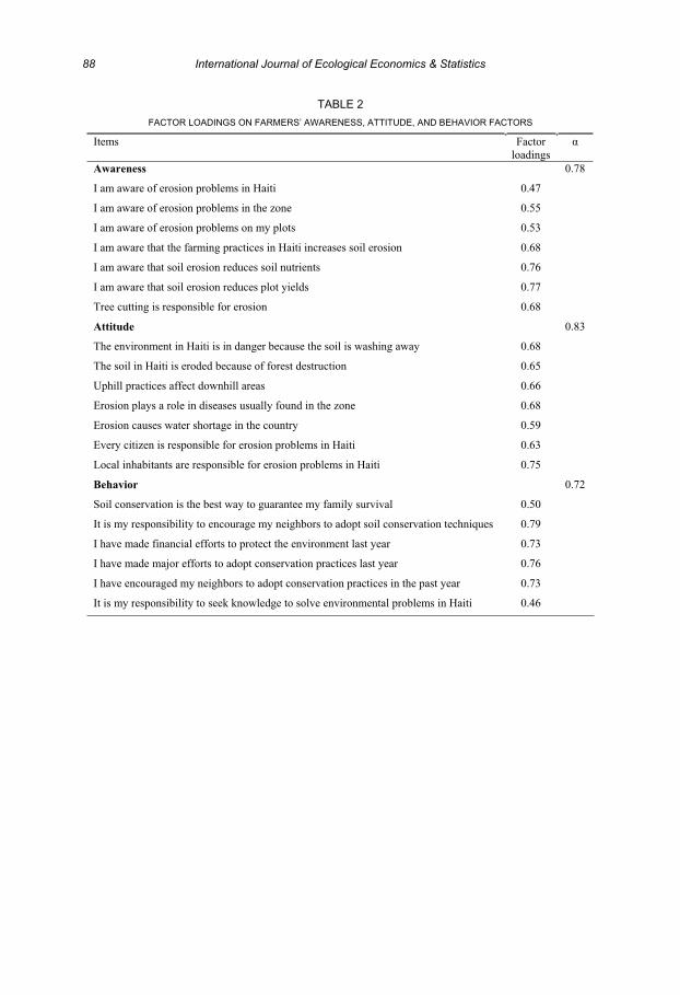
TABLE 2

FACTOR LOADINGS ON FARMERS’ AWARENESS, ATTITUDE, AND BEHAVIOR FACTORS

Items Factor

loadings

Awareness

I am aware of erosion problems in Haiti

I am aware of erosion problems in the zone

I am aware of erosion problems on my plots

I am aware that the farming practices in Haiti increases soil erosion

I am aware that soil erosion reduces soil nutrients

I am aware that soil erosion reduces plot yields

Tree cutting is responsible for erosion

Attitude

The environment in Haiti is in danger because the soil is washing away

The soil in Haiti is eroded because of forest destruction

Uphill practices affect downhill areas

Erosion plays a role in diseases usually found in the zone

Erosion causes water shortage in the country

Every citizen is responsible for erosion problems in Haiti

Local inhabitants are responsible for erosion problems in Haiti

Behavior

Soil conservation is the best way to guarantee my family survival

It is my responsibility to encourage my neighbors to adopt soil conservation techniques

I have made financial efforts to protect the environment last year

I have made major efforts to adopt conservation practices last year

I have encouraged my neighbors to adopt conservation practices in the past year

It is my responsibility to seek knowledge to solve environmental problems in Haiti

0.47

0.55

0.53

0.68

0.76

0.77

0.68

0.68

0.65

0.66

0.68

0.59

0.63

0.75

0.50

0.79

0.73

0.76

0.73

0.46

0.78

0.83

0.72


TABLE 3

PREDICTORS OF ENVIRONMENTAL PERCEPTIONS, AWARENESS, ATTITUDE, AND BEHAVIOR

Path Parameters Standardized

coefficient

t-value

crop dependence susceptibility

land ownership susceptibility

demographic pressure susceptibility

crop dependence severity

land ownership severity

demographic pressure severity

crop dependence barrier

land ownership barrier

demographic pressure barrier

crop dependence benefit

land ownership benefit

demographic pressure benefit

susceptibility awareness

severity awareness

barriers awareness

benefits awareness

crop dependence awareness

land ownership awareness

demographic pressure awareness

susceptibility attitude

severity attitude

barriers attitude

benefits attitude

crop dependence attitude

land ownership attitude

demographic pressure attitude

awareness behavior

attitude behavior

crop dependence behavior

land ownership behavior

demographic pressure behavior

11

12

13

21

22

23

31

32

33

41

42

43

11

12

13

14

15

16

17

21

22

23

24

25

26

27

31

32

33

34

35

0.36*

0.08

0.02

0.20*

-0.13*

0.05

-0.16*

0.12*

-0.08

0.30*

-0.04

0.05

0.24*

0.35*

-0.001

0.06

0.04

-0.13*

-0.07

0.44*

0.22*

-0.04

0.18

0.10*

-0.01

-0.06

0.30*

0.01

0.05

0.09*

0.04

8.25

1.79

0.38

4.32

-2.92

1.01

-3.61

2.74

-1.85

6.97

-1.04

1.07

2.36

5.24

-0.068

0.65

0.78

-2.80

-1.65

4.65

4.18

-0.83

1.94

2.32

-0.17

-1.57

4.32

0.096

0.99

2.01

1.25

Note: *significant at =0.05, 2=669.41, df=265; NFI=0.94, GFI=0.92, CFI=0.96


Pollution in a Spatial Model: Is Zoning a Policy Response?

Yamini Gupt1 and Jacqueline Geoghegan2

1Department of Business EconomicsDelhi University New Delhi, India

Email: [email protected]

2Department of Economics Clark University

Worcester, MA USA Email: [email protected]

Abstract

In this paper a Hotelling spatial model is developed which includes a single firm, that through its production process, creates a pollution externality on all consumers in a linear market. The social optimum location of the firm is derived, taking into account the pollution externality as well as transportation costs. One of the theoretical results is that spatial separation of industrial and residential land uses can be socially optimal, motivating an efficient zoning regulation. This theoretical hypothesis is tested empirically with spatial data on zoning location for a region in Maryland.

Keywords: Hotelling spatial model, pollution externalities, zoning, probit estimation

JEL Classification: Q2, R0, R3


1. INTRODUCTION

One of the original motivations for local land use zoning ordinances was to

separate non-conforming land uses, such as separating residential areas from the

externalities associated with polluting industrial land uses (Pogodzinski and Sass,

1990). From an economic perspective, this non-market solution has the potential to

be inefficient. However, Baumol and Oates (1988) have demonstrated that in a

constant returns to scale linear model of two firms, where one firm increases the

costs of production for the second firm through a pollution externality, if that

externality is strong enough to cause a nonconvexity in the production set, then the

social optimum will be a spatial separation of the two firms. This separation can be


achieved through municipal zoning (Crone, 1983; Fischel, 1994) and this result

suggests that a zoning regulation can be the socially efficient outcome. For

example, Crone (1983) shows that zoning can be efficient by deriving conditions on

relative land prices to indicate externalities strong enough to create non convexities

in production sets. In a trade model, Copeland and Taylor (1999) demonstrate

similar results for the spatial separation of polluting and nonpolluting industries.

This paper follows Baumol and Oates by developing a Hotelling model (1929),

where producers and consumers are distributed along a linear market. Several

authors such as Coase (1960), Wellisz (1964), Nutter (1968), Tybout (1972), and

Marchand and Russel (1973) have used a scenario with a price taking firm imposing

a negative externality on another firm, in their discussions of the Coase theorem.

Among the few authors who have dealt with externalities in an oligopolistic setting,

Levin (1985) analyzes an externality affecting the demand side of the market and

Veendorp and Zambaras (1992) consider Cournot-type oligopolists that generate an

externality that affects all of the firms in the market. Germain (1989) investigates

one duopolist who imposes an externality on another, but the competition among the

duopolists is still of the Cournot type.

The theoretical model presented in this paper is an extension of Gupt and

Veendorp (1997a), where pollution externalities are incorporated into a Hotelling

setting with a polluting upstream duopolist that imposed an externality, in the form of

additional clean up cost on the downstream competitor. Within fixed-price variable-

location (Gupt and Veendorp 1997a) and variable-price variable-location models

(Gupt and Veendorp, 1997b), firm location decisions are modeled. The firms enter

the market in the manner described by Prescott and Visscher (1977). There is a

uniform distribution of consumers along the market who have an inelastic demand

for the good produced by the firms, with the consumers bearing the transportation

costs associated with consuming the good. One of the results for the fixed-price

model is that the firms locate asymmetrically under different liability regimes and

internalization of the externality through taxation is not an effective policy option to

ensure the socially optimal location. Therefore, site regulation is suggested as a

policy option.


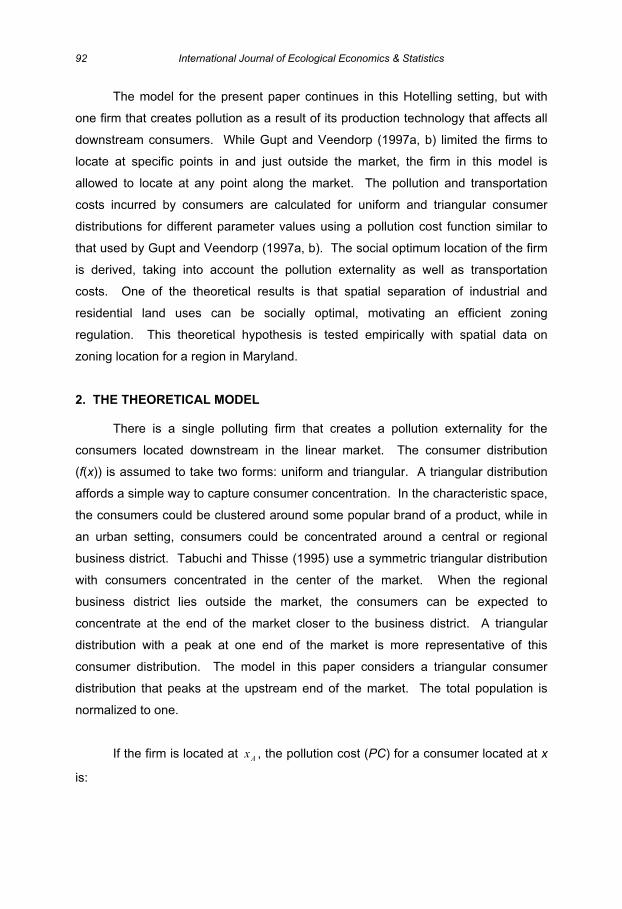
The model for the present paper continues in this Hotelling setting, but with

one firm that creates pollution as a result of its production technology that affects all

downstream consumers. While Gupt and Veendorp (1997a, b) limited the firms to

locate at specific points in and just outside the market, the firm in this model is

allowed to locate at any point along the market. The pollution and transportation

costs incurred by consumers are calculated for uniform and triangular consumer

distributions for different parameter values using a pollution cost function similar to

that used by Gupt and Veendorp (1997a, b). The social optimum location of the firm

is derived, taking into account the pollution externality as well as transportation

costs. One of the theoretical results is that spatial separation of industrial and

residential land uses can be socially optimal, motivating an efficient zoning

regulation. This theoretical hypothesis is tested empirically with spatial data on

zoning location for a region in Maryland.

2. THE THEORETICAL MODEL

There is a single polluting firm that creates a pollution externality for the

consumers located downstream in the linear market. The consumer distribution

(f(x)) is assumed to take two forms: uniform and triangular. A triangular distribution

affords a simple way to capture consumer concentration. In the characteristic space,

the consumers could be clustered around some popular brand of a product, while in

an urban setting, consumers could be concentrated around a central or regional

business district. Tabuchi and Thisse (1995) use a symmetric triangular distribution

with consumers concentrated in the center of the market. When the regional

business district lies outside the market, the consumers can be expected to

concentrate at the end of the market closer to the business district. A triangular

distribution with a peak at one end of the market is more representative of this

consumer distribution. The model in this paper considers a triangular consumer

distribution that peaks at the upstream end of the market. The total population is

normalized to one.

If the firm is located at xA , the pollution cost (PC) for a consumer located at x

is:


0and;)(

kxxxxk

qPC A

A

A (1)

The consumers have a perfectly inelastic demand for the product and since there is

only one firm in the market, it supplies the entire market (i.e. qA = 1). The firm incurs

a zero marginal cost of production. is the pollution cost coefficient which measures

the intensity of pollution and takes on values between zero and one1. The constant k

is included to guarantee that a consumer at the firm’s location2 does not have to face

an infinite level of pollution. Hence, for a consumer at the location of the firm, ( x =

xA ) the pollution cost is k

. A larger value of k would decrease the pollution cost

borne by a consumer located close to the firm.

The transportation cost per unit for each consumer is c multiplied by the

distance between the consumer and the firm. The total transportation cost for all the

consumers located along the market is obtained by integrating the product of c and

this distance over the length of the market. In the next section, an analysis of the

impact of the pollution intensity, the transportation cost, and the type of consumer

distribution on the social cost minimizing location of the firm is performed. Two

cases involving a uniform and a triangular distribution of consumers are considered.

2.1. Uniform Consumer Distribution: f(x) =1

With a uniform consumer distribution, the total transportation cost (TC) for all

consumers is:

1

0

)()(

A

A

x

A

x

A dxxxcdxxxcTC (2)

)(212

AA xccx (3)

1

Lower values of can describe firms that pollute less or use cleaner technologies, while larger values (closer to one)

would correspond to dirty technologies and bigger polluters. 2

This is possible when the firm and the consumer are located opposite each other on two banks of a river.


The total social cost (C) is the sum of the pollution cost (PC) and the transportation

cost (TC):

)(212

1

xcxcdxxxk

C AA

xA

A

(4)

or

)()ln()1ln(212

AAA xccxkxkC (5)

The social cost minimizing first order condition with respect to the location of

the firm requires:

0)12()1(

)(A

AA

xcxkdx

dC (6)

Therefore:

A

Axk

xc1

)12( (7)

The second order condition requires:

0)1(

222

2

AA xkc

dx

Cd (8)

or

cxk A

2)1( 2 (9)

Figure 1 illustrates the effect of various parameters on the social cost

minimizing location of the firm. The value of xA is below (or above) the optimal

location whenever:

0)(0Adx

dTC (10)

or

A

Axk

xc1

)12( (11)


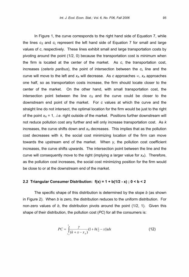
In Figure 1, the curve corresponds to the right hand side of Equation 7, while

the lines cS and cL represent the left hand side of Equation 7 for small and large

values of c, respectively. These lines exhibit small and large transportation costs by

pivoting around the point (1/2, 0) because the transportation cost is minimum when

the firm is located at the center of the market. As c, the transportation cost,

increases (ceteris paribus), the point of intersection between the cL line and the

curve will move to the left and xA will decrease. As c approaches , xA approaches

one half, so as transportation costs increase, the firm should locate closer to the

center of the market. On the other hand, with small transportation cost, the

intersection point between the line cS and the curve could be closer to the

downstream end point of the market. For c values at which the curve and the

straight line do not intersect, the optimal location for the firm would be just to the right

of the point xA = 1, .i.e. right outside of the market. Positions further downstream will

not reduce pollution cost any further and will only increase transportation cost. As k

increases, the curve shifts down and xA decreases. This implies that as the pollution

cost decreases with k, the social cost minimizing location of the firm can move

towards the upstream end of the market. When , the pollution cost coefficient

increases, the curve shifts upwards. The intersection point between the line and the

curve will consequently move to the right (implying a larger value for xA). Therefore,

as the pollution cost increases, the social cost minimizing position for the firm would

be close to or at the downstream end of the market.

2.2 Triangular Consumer Distribution: f(x) = 1 + b(1/2 - x) ; 0 < b < 2

The specific shape of this distribution is determined by the slope b (as shown

in Figure 2). When b is zero, the distribution reduces to the uniform distribution. For

non-zero values of b, the distribution pivots around the point (1/2, 1). Given this

shape of their distribution, the pollution cost (PC) for all the consumers is:

dxxbxxk

PC

Ax A

))(1()(

21

1

(12)


)1(1

ln)](1[21

AA

A xbk

xkkxb (13)

When b=0, the lower extreme, the pollution cost is similar to the case where the

consumer distribution is uniform:

k

xkPC A1

ln (14)

When b=2, the upper extreme, the pollution cost is:

)1(21

ln)1(2 AA

A xk

xkkxPC (15)

The pollution cost is at a minimum (zero) when the firm locates at the downstream

end of the market (i.e., at xA=1) irrespective of the value of b or any other parameter.

The sum of the transportation cost (TC) over all consumers is:

A

A

x

x

AA dxxbxxcdxxbxxcTC0

1

21

21 ))(1)(())(1)(( (16)

})1({122

12

2

3

3b

AAb

Ab xxxc (17)

When b=0, the total transportation cost incurred by the consumers is:

)(212

AA xccxTC (18)

For this type of uniform consumer distribution, the transportation cost minimizing

location of the firm will be the center of the market, i.e. where xA =1/2. As the value

of b approaches 2, the transportation cost is minimized at firm locations closer to the

upstream end of the market. When b =2 and the consumer distribution has a peak at

the upstream end of the market, the total transportation cost is minimum when the

firm’s location, xA, is 0.29.


The total social cost C is:

)1()1

ln()](1[21

AA

A xbk

xkkxb + })1({

12212

2

3

3b

AAb

Ab xxxc (19)

The first order condition to minimize this cost with respect to the location of the firm

is:

0}1)2({]1)([1

)1

ln1( 2

21

AAA

A

A

A

xbbxckxbxkk

xkb

x

C (20)

The second order condition for an interior minimum requires:

0}22{1

2

)1(]1)([

221

2

2

bbxcxk

b

xkkxb

x

CA

AA

A

A

(21)

From the first order condition, when k=1 and b=0

}12{}2

1{ A

A

xcx

(22)

This result is a special case of that shown in Figure 1. The other possible extreme is

when b=2 and k=1:

}124{)}2ln(2{ 2

AAA xxcx (23)

Figure 3 shows the effect of different values of the parameters on the social

cost minimizing location of the firm from Equation 23. In the special case when c

and have a unit value, which is shown in Figure 3, (with the c=1 curve as the right

hand side of Equation 23, and =1 represents the left hand side) the line and the

curve intersect to the right of the center of the market, near xA = 0.6. For this


combination of the parameter values, the firm can be located closer to the center of

the market to minimize the total cost to society. When the transportation cost

increases (ceteris paribus), the curve c = 1 will pivot upwards around the point xA =

0.29, and the intersection point between the curves will move to the left3. The social

cost minimizing location of the firm will be closer to the upstream end of the market.

On the other hand, the curve = 1 will pivot upwards around xA = 1 and the

intersection point will move to the right when the pollution intensity increases. This

means that when the pollution cost increases, the firm should be located closer to

the downstream end of the market in order to minimize total social cost.

As can be seen from Figure 1, the socially optimal location for the polluting

firm will be close to or at the downstream end of the market, for certain combinations

of the parameter values , k, c and b, whether the model assumes a uniform or a

triangular consumer distribution. These results are consistent with the observation

that communities have an incentive to adopt a “beggar-thy-neighbor” policy and

locate dirty industries close to their borders or downwind/downstream to save

themselves from the imminent pollution (Fischel, 1985). In this way, local regulators

minimize the social cost to their constituents, by passing on the pollution to

neighboring localities. In the following section, tests of the hypothesis if local

regulators are more likely to permit industrial land uses closer to their borders are

performed, using spatially-explicit zoning and other data in a geographical

information system (GIS) framework.

3. Econometrics

3.1. Data

The spatially-explicit zoning data are for seven counties in Maryland: Anne

Arundel, Calvert, Charles, Howard, Montgomery, Prince George’s, and St. Mary’s.

This geographical region covers about one thousand square miles. Approximately

50 percent of this area is covered by natural vegetation, 30 percent is occupied by

agricultural land uses, 15 percent by residential land uses and industrial land uses

3 Which is one of the roots to the quadratic equation of the right hand side of Equation 23. The other root is xA =

1.7, which is not considered here as it is outside the length of the market.


occupy about 5 percent of the area (Bockstael, 1996). The study area borders

Washington D.C. and includes Annapolis, the state capital, located in Anne Arundel

county. The zoning data are from the Maryland Office of Planning and reflect the

zoning for these counties in 1995. Zoning is regulated at the county level in

Maryland. In addition, other spatially-explicit data include information on the road

network and data from the 1990 Population Census.

The dependent variable for the econometric model was created from these

digital zoning maps, aggregated into two categories: “dirty” (industrial) and “clean”

(residential, commercial, agricultural, forestry). To standardize the unit of

observation, a grid of 50m by 50m was drawn over the zoning map. To reduce the

number of observations, the data were resampled to a coarser resolution of 150m by

150m. The explanatory variables from the Census and other digital maps were then

linked to the 150m observation through GIS.

3.2. Hypotheses

The results of the theoretical section of this paper suggest that local planners

have an incentive to locate dirty land uses close to their boundaries. To test this

hypothesis if planners are more likely to zone industrial land uses closer to their

borders, controlling for other features, a probit model was estimated with “dirty” and

“clean” zoning as the dependent variable. The distance for each observation to the

land boundary (landist) and water boundary (watdist) of the county was calculated, to

use in a test of if distant to land boundary decreases the probability of an observation

being zoned “dirty”. A distinction is made between the land and water boundaries to

account for possible efforts made by planners to maintain the pristine quality of water

bodies. These efforts could be motivated by their concern for environmental

preservation or to maintain the residential land value of expensive water front

property.

Other controls included in the model that are expected to affect the probability

of being zoned “dirty” are: distance to nearest major road (rdist); distance to the

central business district of Washington D.C. (wdcdist); population density in the block

group that the observation fall in (popden). The wdcdist and rdist variables are


proxies for the effect of the transportation cost coefficient (c) on zoning decisions

from the theoretical model, and popden captures the effect of the pollution intensity

( ). The a priori hypotheses on the control variables are that rdist and wdcdist will

each have a negative effect on the probability of being zoned “dirty”, as these

capture the transportation costs of doing business, and popden is also hypothesized

to negatively influence the probability of being zoned “dirty”, as planners often keep

non-conforming land uses apart.

The type of neighborhood an observation is located in could potentially also

affect its probability of being zoned “dirty” or not, for example due to agglomeration

effects. Industrial firms might wish to locate near each other or planners may want to

concentrate polluting industries in a specific area to keep the other parts of their

jurisdiction “clean.” In order to capture this effect a neighborhood variable was

calculated (nbhd), where a neighborhood was considered “dirty” if a majority of the

surrounding nearest observations were also zoned “dirty”. Landis and Zhang (1998)

use a similar measure of neighborhood effects in their study of the determinants of

land-use change in a discrete choice model. Case (1992) finds that ignoring such

neighborhood effects may bias the estimation of parameters of interest.

3.3. Empirical Specification

It is assumed that there is a linear function of the explanatory variables that is

an index of industrial potential I of that observations(Greene,1997; Gujarati,1995):

iiii xI ' (24)

Where the xi are explanatory variables, and the and are parameters to be

estimated, and µ is an unobserved error term. Ii is unobservable, however y is

observed where:

y =1 if Ii > Ii*

y = 0 otherwise (25)


That is, if the index of industrial potential for an observation exceeds a certain critical

value Ii*, the observation will be observed to be zoned “dirty” and otherwise it will be

zoned “clean”. If the errors are assumed to be independently and identically

distributed normally, then the specification becomes a probit model. In the model

estimated below, each explanatory variable is interacted with a county dummy to

allow for the effects to differ by county, as zoning regulations are set in Maryland at

the county level. County dummies are also included to control for unobserved

variation in the quality of public goods, tax rates, crime rates, etc. that vary at the

county level. The variables and their summary statistics can be found in Table 1.

3.4. Estimation and Results

The estimated coefficients and their significance levels from the econometric

model are found in Table 2. There are mixed results for the main variable of interest,

the distance to the land border of the county (landist). For three out of the seven

counties (Calvert, Charles, Howard), the estimated coefficient is negative and

statistically significant, implying that holding all else constant, an increase in the

distance from the land border for these counties decreases the probability that the

observation will be zoned industrial, the result that was hypothesized from the

theoretical mode. For three of the counties (Anne Arundel, Montgomery, Prince

George’s), this variable is not statistically different from zero and for one county (St

Mary’s) the estimated coefficient was positive and significant. Perhaps these results

are because Anne Arundel, Montgomery, and Prince George’s were developed

much earlier than the other counties, so that much of their current industrial zones

are grandfathered land uses.

Turning to the control variables, most of the empirical results are consistent

with the a priori expectations. For two of the counties (Anne Arundel, Prince

George’s), the distance to the water boundary (watdist) was positive and significant,

so that these counties appear to keep industrial zones away from their water

boundaries, while for the remaining counties, the estimated coefficients were not

statistically different from zero. The distance to roads (rdist) and distance to

Washington D.C. (wdcdist) variables act as proxies for the transportation cost

coefficient from the theoretical model. The proximity to major roads plays an


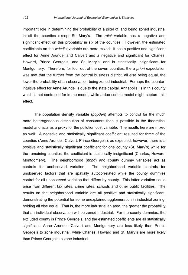
important role in determining the probability of a pixel of land being zoned industrial

in all the counties except St. Mary’s. The rdist variable has a negative and

significant effect on this probability in six of the counties. However, the estimated

coefficients on the wdcdist variable are more mixed. It has a positive and significant

effect for Anne Arundel and Calvert and a negative and significant for Charles,

Howard, Prince George’s, and St. Mary’s, and is statistically insignificant for

Montgomery. Therefore, for four out of the seven counties, the a priori expectation

was met that the further from the central business district, all else being equal, the

lower the probability of an observation being zoned industrial. Perhaps the counter-

intuitive effect for Anne Arundel is due to the state capital, Annapolis, is in this county

which is not controlled for in the model, while a duo-centric model might capture this

effect.

The population density variable (popden) attempts to control for the much

more heterogeneous distribution of consumers than is possible in the theoretical

model and acts as a proxy for the pollution cost variable. The results here are mixed

as well. A negative and statistically significant coefficient resulted for three of the

counties (Anne Arundel, Calvert, Prince George’s), as expected, however, there is a

positive and statistically significant coefficient for one county (St. Mary’s) while for

the remaining counties, the coefficient is statistically insignificant (Charles, Howard,

Montgomery). The neighborhood (nbhd) and county dummy variables act as

controls for unobserved variation. The neighborhood variable controls for

unobserved factors that are spatially autocorrelated while the county dummies

control for all unobserved variation that differs by county. This latter variation could

arise from different tax rates, crime rates, schools and other public facilities. The

results on the neighborhood variable are all positive and statistically significant,

demonstrating the potential for some unexplained agglomeration in industrial zoning,

holding all else equal. That is, the more industrial an area, the greater the probability

that an individual observation will be zoned industrial. For the county dummies, the

excluded county is Prince George’s, and the estimated coefficients are all statistically

significant: Anne Arundel, Calvert and Montgomery are less likely than Prince

George’s to zone industrial, while Charles, Howard and St. Mary’s are more likely

than Prince George’s to zone industrial.


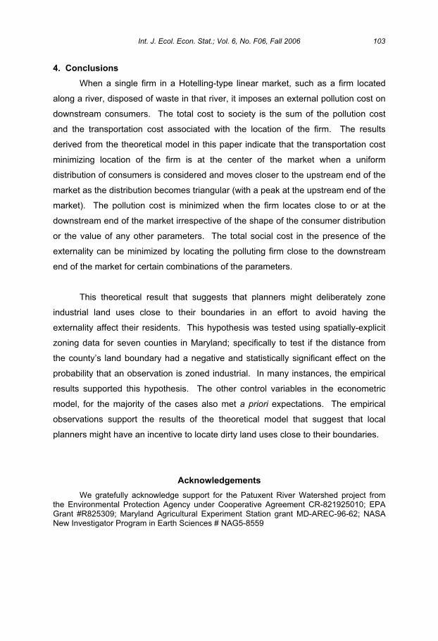
4. Conclusions

When a single firm in a Hotelling-type linear market, such as a firm located

along a river, disposed of waste in that river, it imposes an external pollution cost on

downstream consumers. The total cost to society is the sum of the pollution cost

and the transportation cost associated with the location of the firm. The results

derived from the theoretical model in this paper indicate that the transportation cost

minimizing location of the firm is at the center of the market when a uniform

distribution of consumers is considered and moves closer to the upstream end of the

market as the distribution becomes triangular (with a peak at the upstream end of the

market). The pollution cost is minimized when the firm locates close to or at the

downstream end of the market irrespective of the shape of the consumer distribution

or the value of any other parameters. The total social cost in the presence of the

externality can be minimized by locating the polluting firm close to the downstream

end of the market for certain combinations of the parameters.

This theoretical result that suggests that planners might deliberately zone

industrial land uses close to their boundaries in an effort to avoid having the

externality affect their residents. This hypothesis was tested using spatially-explicit

zoning data for seven counties in Maryland; specifically to test if the distance from

the county’s land boundary had a negative and statistically significant effect on the

probability that an observation is zoned industrial. In many instances, the empirical

results supported this hypothesis. The other control variables in the econometric

model, for the majority of the cases also met a priori expectations. The empirical

observations support the results of the theoretical model that suggest that local

planners might have an incentive to locate dirty land uses close to their boundaries.

Acknowledgements

We gratefully acknowledge support for the Patuxent River Watershed project from the Environmental Protection Agency under Cooperative Agreement CR-821925010; EPA Grant #R825309; Maryland Agricultural Experiment Station grant MD-AREC-96-62; NASA New Investigator Program in Earth Sciences # NAG5-8559


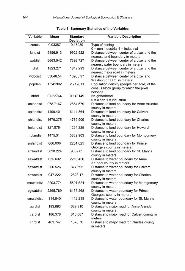
Table 1: Summary Statistics of the Variables

Variable Mean Standard Deviation

Variable Description

zones 0.03387 0.18089 Type of zoning 0 = non industrial 1 = industrial

landist 9856.913 9922.522 Distance between center of a pixel and the nearest land boundary in meters

watdist 6663.542 7392.727 Distance between center of a pixel and the nearest water boundary in meters

rdist 1823.271 1849.293 Distance between center of a pixel and the nearest major road in meters

wdcdist 33648.54 18980.97 Distance between center of a pixel and Washington D.C. in meters

popden 1.341902 2.712811 Population density (people per acre) of the census block group to which the pixel belongs

nbhd 0.022764 0.149149 Neighborhood 0 = clean 1 = industrial

aalandist 978.7167 2864.579 Distance to land boundary for Anne Arundel county in meters

calandist 1499.401 6114.864 Distance to land boundary for Calvert county in meters

chlandist 1679.375 4789.909 Distance to land boundary for Charles county in meters

holandist 327.8764 1264.225 Distance to land boundary for Howard county in meters

molandist 1475.314 3882.903 Distance to land boundary for Montgomery county in meters

pglandist 866.006 2251.625 Distance to land boundary for Prince George’s county in meters

smlandist 3030.224 9332.05 Distance to land boundary for St. Mary’s county in meters

aawatdist 635.692 2216.456 Distance to water boundary for Anne Arundel county in meters

cawatdist 206.526 877.595 Distance to water boundary for Calvert county in meters

chwatdist 947.222 2823.17 Distance to water boundary for Charles county in meters

mowatdist 2293.774 5891.524 Distance to water boundary for Montgomery county in meters

pgwatdist 2265.789 6133.268 Distance to water boundary for Prince George’s county in meters

smwatdist 314.540 1112.218 Distance to water boundary for St. Mary’s county in meters

aardist 193.693 629.310 Distance to major road for Anne Arundel county in meters

cardist 186.378 818.087 Distance to major road for Calvert county in meters

chrdist 463.747 1378.76 Distance to major road for Charles county in meters


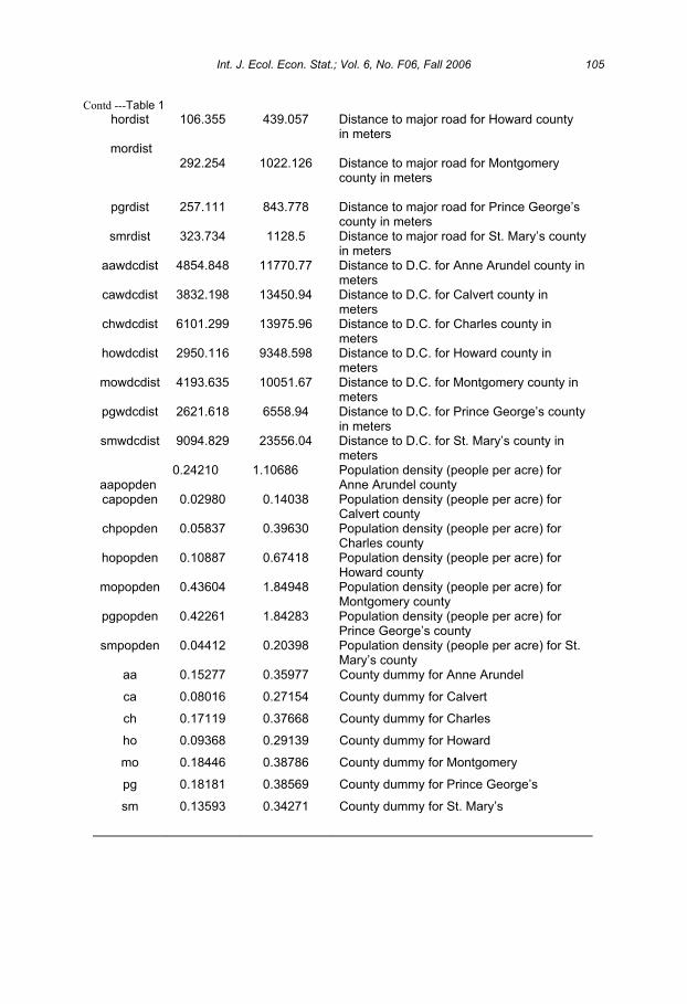
Contd ---Table 1

hordist 106.355 439.057 Distance to major road for Howard county in meters

mordist 292.254 1022.126 Distance to major road for Montgomery

county in meters

pgrdist 257.111 843.778 Distance to major road for Prince George’s county in meters

smrdist 323.734 1128.5 Distance to major road for St. Mary’s county in meters

aawdcdist 4854.848 11770.77 Distance to D.C. for Anne Arundel county in meters

cawdcdist 3832.198 13450.94 Distance to D.C. for Calvert county in meters

chwdcdist 6101.299 13975.96 Distance to D.C. for Charles county in meters

howdcdist 2950.116 9348.598 Distance to D.C. for Howard county in meters

mowdcdist 4193.635 10051.67 Distance to D.C. for Montgomery county in meters

pgwdcdist 2621.618 6558.94 Distance to D.C. for Prince George’s county in meters

smwdcdist 9094.829 23556.04 Distance to D.C. for St. Mary’s county in meters

aapopden0.24210 1.10686 Population density (people per acre) for

Anne Arundel county capopden 0.02980 0.14038 Population density (people per acre) for

Calvert county chpopden 0.05837 0.39630 Population density (people per acre) for

Charles county hopopden 0.10887 0.67418 Population density (people per acre) for

Howard county mopopden 0.43604 1.84948 Population density (people per acre) for

Montgomery county pgpopden 0.42261 1.84283 Population density (people per acre) for

Prince George’s county smpopden 0.04412 0.20398 Population density (people per acre) for St.

Mary’s county aa 0.15277 0.35977 County dummy for Anne Arundel

ca 0.08016 0.27154 County dummy for Calvert

ch 0.17119 0.37668 County dummy for Charles

ho 0.09368 0.29139 County dummy for Howard

mo 0.18446 0.38786 County dummy for Montgomery

pg 0.18181 0.38569 County dummy for Prince George’s

sm 0.13593 0.34271 County dummy for St. Mary’s


Table 2: Econometric Results, Probit model, dependent variable, zoning (industrial or not) n=309,884 Pseudo R2 = 0.7444

VariableName

EstimatedCoefficient

t-statistic Variable Name

EstimatedCoefficient

t- statistic

aanbhd 3.428* 70.942 hordist -4.96e-04* -9.51

canbhd 4.467* 26.973 mordist -1.89e-04* -6.66

chnbhd 4.212* 44.414 pgrdist -2.17e-04* -9.95

honbhd 4.082* 48.891 smrdist 2.67e-05 1.46

monbhd 4.244* 57.231 aawdcdist 6.56e-05* 19.37

pgnbhd 4.149* 83.975 cawdcdist 7.88e-05* 4.92

smnbhd 4.862* 28.019 chwdcdist -2.61e-05* -7.20

aalandist -1.04e-05 -1.95 howdcdist -2.09e-05* -5.13

calandist -7.82e-05* -4.73 mowdcdist -2.39e-06 -0.97

chlandist -1.82e-05* -3.60 pgwdcdist -1.76e-05* -6.81

holandist -2.14e-04* -11.34 smwdcdist -1.39e-04* -4.30

molandist 7.16e-06 1.69 aapopden -0.102* -8.68

pglandist -1.24e-06 -0.23 capopden -0.756* -3.80

smlandist 1.47e-04* 4.45 chpopden -0.026 -1.20

aawatdist 9.15e-05* 14.25 hopopden 0.006 0.35

cawatdist 1.11e-05 0.36 mopopden -0.006 -0.90

chwatdist 5.87e-06 1.11 pgpopden -0.034* -5.98

mowatdist -3.85e-06 -1.12 smpopden 0.181* 6.57

pgwatdist 8.53e-06* 4.64 aa -2.671* -16.02

smwatdist 2.1e-05 0.83 ca -2.371* -4.31

aardist -6.6e-05* -4.48 ch 0.695* 4.43

cardist -4.98e-04* -7.21 ho 0.986* 6.38

chrdist -2.62e-04* -12.03 mo -0.474* -4.37

constant -1.887* -29.66 sm 4.785* 3.32

* significant at the 5% level


Figure 1 The relationship between the pollution cost, the transportation cost and the

social cost minimizing location of the firm.


Figure 2 The triangular consumer distribution


Figure 3 The effect of c and on the social cost minimizing location of the firm. c= =1


References

Bockstael, Nancy E., 1996, Modeling Economics and Ecology: The Importance of a Spatial Perspective, American Journal of Agricultural Economics, 78, 1168-1180.

Baumol, William J. and Wallace E. Oates, 1988, Theory of Environmental Policy,Second Edition, Cambridge University Press, Cambridge, England.

Case, Anne, 1992, Neighborhood Influence and Technological Change, RegionalScience andUrban Economics, 22, 491-508.

Copeland, Brian R. and M. Scott Taylor, 1999, Trade, Spatial Separation, and the Environment, Journal of International Economics, 47, 137-168.

Crone, Theodore M., 1983, Elements of an Economic Justification for Municipal Zoning, Journal of Urban Economics, 14, 168-83.

Fischel, William A., 1975, Fiscal and Environmental Considerations in the Location ofFirms in Suburban Communities. In E. Mills and W. Oates (eds.), Fiscal Zoning and Land Use Control, Lexington Books, Lexington, MA.

Fischel, William A., 1985, The Economics of Zoning Laws: A Property RightsApproach to American Land Use Controls, Johns Hopkins University Press, Baltimore, MD.

Fischel, William A., 1994, Zoning, Nonconvexities, and T. Jack Foster’s City,Journalof Urban Economics, 35, 175-81.

Gujarati, Damodar N., 1995, Basic Econometrics (3rd edition), McGraw-Hill Inc., New York.

Gupt, Yamini and E.C.H. Veendorp, 1997a, Externalities in a Hotelling Model, Southern Economic Journal, 64,1, 321-325.

Gupt, Yamini and E.C.H. Veendorp, 1997b, Competition in a Linear Market with Externalities. In Our Natural Environment: At a Crossroad, Proceedings for the 3rd

International Interdisciplinary Conference on the Environment, Cambridge, MA.

Hotelling, H., 1929, Stability in Competition, The Economic Journal, 39, 41-57.

Landis J., and M. Zhang, 1998, The second generation of the California urban futures model. Part 2: Specification and calibration results of the land-use change submodel, Environment and Planning B: Planning and Design, 25, 795-824.

Pogodzinski, Michael and Tim R. Sass, 1990, The Economic Theory of Zoning: A Critical Review, Land Economics, 66, 3, 294-314.


Prescott, E.C., and M. Visscher, 1977, Sequential Location Among Firms With Foresight, Bell Journal of Economics and Management Science, 8, 378-393.

Tabuchi, T. and J.-F. Thisse, 1995, Asymmetric Equilibria in Spatial Competition. International Journal of Industrial Organization, 13, 2, 213-227.


Submission of Manuscripts

International Journal of Ecological Economics & Statistics

ISSN 0973-1385

The authors should submit a complete hard copy of manuscript (with an electronic copy) of their unpublished and original paper to the Editor-in-Chief, International Journal of Ecological Economics & Statistics (IJEES), Centre for Environment, Social & Economic Research, Post Box No. 113, Roorkee-247667, INDIA; Email: [email protected]; [email protected] will be assume that authors will keep a copy of their paper. We strongly encourage electronic submission of manuscript by email to the Editor-in-Chief IJEES. IJEES is published one Volume per year, three issues yearly in Winter, Summer and Fall by Centre for Environment, Social & Economic Research, Post Box No. 113, Roorkee-247667, INDIA.Instructions for author are also available at http://ceser.res.in/ijees/instr4a.html.

Format of Manuscripts:

Please send your paper as a single document including tables and figures. This means, it should be one Microsoft Word file ... AND NOT a zipped File containing different files for text, tables, figures, etc.

The paper should not normally exceed 5000 words, and should conform to the following:

Cover page giving title, author(s), affiliation(s), mailing address and e-mail address All pages should be without page number, header Text and footer text. Abstract describing the context and scope of the paper Keywords

JEL / Mathematics Subject Classification Main text References

The manuscript should be in the following format-

Page Size A4 (8.27” x 11.69”) without page number

Page Margin Top=1.0 inch, Bottom=1.0 inch

Left=1.0”, Right=1.0”

Font Face Times New Roman

Font Size for Title 16 pt. Bold & Title Case

Font Size for Headings 12 pt. Bold & CAPITAL CASE

Font Size for Sub-Headings 12 pt. Bold & Title Case

Alignment for Title & Headings Center

Font size for Text 12 pt.

Line Space for Text 1.5 line space

Paragraph No Tab, and 12 pt. Space after paragraph & Alignment=Justify

Abstract & Keyword Paragraph Margin: Right=0.5”, Left=0.5”,

Font: size=10 pt.

Font Face =Arial & Italic

Align= justify

Paragraph Line Space=single

Reference Align= justify

Line Space=single and 10 pt. space before the next reference.

Table and Figures Should be separate and at the last of manuscript. Line space=single

Submission of a paper implies that the reported work is neither under consideration for a

scientific journal nor already published. All manuscripts are subject to peer review. If

revisions are required for acceptance of a manuscript, one copy of the revised manuscript

should be submitted.

Print copy of the journal will be dispatch to subscribers only. However, authors will get the e-

issue of journal without any payment. A free print (paper) issue of journal will be available to

the authors whose institutions subscribe. A copy of single issue of journal is available on a

special discount to the authors only. Furthermore, you are welcome to support the journal by

requesting that your library to subscribe the journal, or by taking out an individual

subscription.

Preparation of the Manuscript

Papers must be clearly written in English. All sections of the manuscript should be typed,

double-spaced, on one side of the paper only. In addition to the full title of the paper, authors

should supply a running title, of less than 40 characters, and up to five keywords.

Research papers should be accompanied by an abstract, which will appear in front of the

main body of the text. It should be written in complete sentences and should summarize the

aims, methods, results and conclusions in less than 250 words. The abstract should be

comprehensible to readers before they read the paper, and abbreviations and citations

should be avoided.

Authors are responsible for the accuracy of references. Within the text, references should be

cited by author's name(s) and year of publication (where there are more than two authors

please use et al.). Published articles and those in press (state the journal which has

accepted them and enclose a copy of the manuscript) may be included. Citations should be

typed at the end of the manuscript in alphabetical order, with authors' surnames and initials

inverted. References should include, in the following order: authors' names, year, paper title,

journal title, volume number, issue number, inclusive page numbers and (for books only)

name and address of publishers. References should therefore be listed as follows:

Natterer, F., 1986, The Mathematics of Computerized Tomography, John Wiley & Sons, New York.

Herman, G.T., 1972, Two Direct Methods for Reconstructing Pictures from their Projections: A Comparative Study, Computer Graphics and Image Processing, 1, 123-144.

Dasgupta. P., 2003, Population, Poverty, and the Natural Environment. in Mäler K.-G. and Vincent, J. (Eds.), Handbook of Environmental and Resource Economics, Amsterdam: North Holland.

Levin, S.A., Grenfell, B., Hastings, A., and Perelson. A.S. 1997, Mathematical and Computational Challenges in Population Biology and Ecosystem Science, Science, 275, 334-343.

Tables should be self-explanatory and should include a brief descriptive title. Illustrations

should be clearly lettered and of the highest quality. Acknowledgements and Footnotes

should be included at the end of the text. Any footnote should be identified by superscripted

numbers.

International Journal of Ecological Economics & Statistics

ISSN 0973-1385

http://www.ceser.res.in/ijees.html

SUBSCRIPTIONS

Followings are the Annual Subscription rate for (a volume) year 2006:

Issue Individual Library

Print Issue: Euro € /US$ 350.00 Euro € /US$ 450.00

Online: Euro € /US$ 300.00 Euro € /US$ 450.00

Print Issue & Online (Both): Euro € /US$ 450.00 Euro € /US$ 650.00

Subscriptions in India? Please subtract Euro/US$ 30.00 for print issue (postage+handling charges).

How to Pay Subscriptions?

Subscriptions are payable in advance. Subscribers are requested to send payment with their order. Issues will only be sent on receipt of payment. Subscriptions are entered on an annual basis and may be paid in Rupees or US Dollars.

Euro / US Dollar for rates apply to subscribers in all countries except the India where the Rupees rate is applicable.

Payment can be made by Bank Draft/Cheque/ Bank Wire Transfers (please add Euro / US $ 25 as cheque transfer charges, in case of cheque) only. All payments should be made to "Centre for Environment, Social & Economic Research" bank draft/Cheque should be drawn on a Roorkee, India.

Claims and Cancellations

Claims for issues not received should be made in writing within three months of

the date of publication. Cancellations: no refunds will be made after the first issue

of the journal for the year has been dispatched.

Send your subscription to the Editor-in-Chief or Executive Editor.

Detailed information and instructions are available at

http://www.ceser.res.in/ijees.html

Date post:	18-Apr-2018
Category:	Documents
Upload:	trandang
View:	217 times
Download:	4 times

Professor Charles Perringsperrings.faculty.asu.edu/pdf_papers_Perrings/Perrings_IJEES_(2006).pdfAlaa...

Documents