Professur f ¨ ur Hydrologie der Albert-Ludwigs-Universit¨ at Freiburg i. Br Moritz M¨ ahrlein Streamflow response to forest fire and salvage harvesting in a snow dominated catchment: a model-based change detection approach Supervisor: Prof. Dr. Markus Weiler (Albert-Ludwigs-Universit¨ at Freiburg) Co-Supervisor: Prof Dr. Dan Moore (University of British Columbia) Master Thesis July 2016
Transcript
Professur fur Hydrologieder Albert-Ludwigs-Universitat Freiburg i. Br
Moritz Mahrlein
Streamflow response to forest fire and salvage harvesting
in a snow dominated catchment:
a model-based change detection approach
Supervisor: Prof. Dr. Markus Weiler (Albert-Ludwigs-Universitat Freiburg)
Co-Supervisor: Prof Dr. Dan Moore (University of British Columbia)
Master Thesis
July 2016
Declaration of Authorship
I, Moritz Mahrlein, hereby declare the originality of this thesis. I confirm that the
presented work is my own, that all work of others is quoted properly and that I have
acknowledged all main sources of my help.
Vancouver, 10th of July 2016
Abstract
Forest fires affect hydrology in number of ways ranging from making the soil hydropho-
bic to removing the canopy and thus raising energy inputs to a below-canopy surface.
There is a range of approaches to study the impact of canopy removal on streamflow.
In this study, a model based change detection approach was implemented in order to
evaluate the impact of the McLure Forest Fire on the streamflow of Fishtrap Creek,
which burned 60% of the catchment in the summer of 2003. Following the fire, the
burned area was salvage logged. Apart from the change detection, a second aim was to
evaluate the uncertainty linked to the change of forest cover through time. Six different
land cover data sets representing forest cover for the whole pre-fire study period from
1970 to 2003 were used to calibrate an HBV-EC model family for Fishtrap Creek using
two different calibration algorithms. By comparing resultant calibrated parameter sets,
it was shown that the different calibration sets led to a substantial variability in pa-
rameters. This indicates that the specification of land cover can be a significant source
of parameter uncertainty. The model with the best performance was then selected to
be used in the change detection analysis. For this purpose, a regression model was
fitted between observed and simulated discharge using only pre-fire data. With the
help of this regression model post-fire streamflow was predicted in order to simulate a
non disturbed runoff. By comparing the simulated and observed time series, an earlier
onset of the melt seasons with no increase in peak flows was identified, with a higher
consistency following the salvage logging. Two more regression models were set up in
order to test the effect of the fire statistically. The ”full” model accounted for the effect
of the period (pre-fire and post-fire), the ”reduced” model was based on the discharge
values. When comparing them by an ANOVA, two main periods of change were iden-
tified: early winter linked to pre-harvest runoff events and early spring freshet linked
to post-harvest events. Apart from these melt dominated seasons, no change in runoff
was detected.
Zusammenfassung
Waldbrande beeinflussen die Hydrologie eines Einzugsgebietes in verschiedenster Weise,
von der Hydrophobisierung der Boden bis hin zum Entfernen der Baumkrone, wodurch
eine erhohte Energiezufuhr in das System ermoglicht wird. Es existieren viele verschie-
dene Methoden, um die Auswirkungen von Waldbranden und Holzernte zu untersuchen.
In dieser Masterarbeit wird ein modellbasiertes Verfahren angewendet um die Ande-
rung im Abfluss nach einem Waldbrand zu evaluieren. Es werden die Auswirkungen
des McLure Forest Fires auf das Einzugsgebiet des Fishtrap Creek untersucht, welches
im Jahr 2003 zu 60% abbrannte. In den folgenden zwei Jahren wurde das Einzugsge-
biet zusatzlich zu dem Waldbrand, durch das Abernten der verbrannten Flachen noch
weiter beeinflusst. Neben dieser Evaluation wurde in der vorliegenden Arbeit die Aus-
wirkung von veranderter Landnutzung wahrend des Modellierungszeitraumes auf die
Modellperformance untersucht. Hierfur wurden sechs verschiedene Landnutzungsdaten-
satze, die den gesamten Modellierungszeitraum von 1970 bis 2003 abdecken, genutzt
um mithilfe zweier verschiedener Algorithmen eine HBV-EC basierte Modellfamilie zu
kalibrieren. Im Vergleich der kalibrierten Parametersatze zeigte sich eine hohe Varia-
bilitat die mit den verschiedenen Landnutzungsdaten verknupft werden kann und als
bisher nicht untersuchte Ursache fur Parameterunsicherheit interpretiert wurde. Um
die Anderungen im Abfluss zu evaluieren, wurde das am besten kalibrierte Modell aus
der Modellfamilie gewahlt. Anhand dessen wurde ein Regressionsmodel zwischen den
observierten und simulierten Daten auf den Zeitraum vor dem Waldbrand kalibriert.
Mithilfe dieses Modells wurde fur den Zeitraum nach dem Waldbrand Abfluss fur ein
ungestortes Einzugsgebiet simuliert. Im Vergleich des simulierten Abflusses mit dem
gemessenen Abfluss konnte eine vorzeitige schmelzwasserdominierte Hochwasserspitze
ausgemacht werden. Eine Vergroßerung des maximalen Abflusses wurde nicht sichtbar.
Dieser Effekt zeigte sich verstarkt nach dem die Waldbrandflachen abgeholzt wurden.
Anhand zwei weiterer Regressionsmodelle wurde die Auswirkung des Waldbrandes sta-
tistisch uberpruft. Eine ANOVA wurde zwischen den beiden Modellen durchgefuhrt,
wobei ein Modell den Einfluss des Zeitraumes (vor dem Waldbrand im Vergleich zu
nach dem Waldbrand) berucksichtigte, wahrend das zweite lediglich den Zusammen-
hang zwischen Abflussen berucksichtigt. Hier zeigte sich, dass besonders zwei Zeitraume
beeinflusst wurden: im fruhen Winter passend zu den erhohten Abflussen vor der Ab-
holzung und der Zeitraum der vorzeitigen Schmelzwasserabflusse im Fruhling. Neben
diesen beiden Perioden zeigte die statische Auswirkung keine weiteren beeinflussten
Zeitraume.
Acknowledgements
First and foremost, I would like to thank my supervisor Prof. Dr. Markus Weiler for
making this thesis possible. A special thanks goes to my co-supervisor Prof. Dr. Dan
Moore for his support, enthusiasm and his answers to all my questions.
Furthermore, I would like to thank my friends and family for supporting me during
the thesis, everyone doing their best to help me. I would especially like to thank my
parents, without whose financial support and patience I would not have been able to
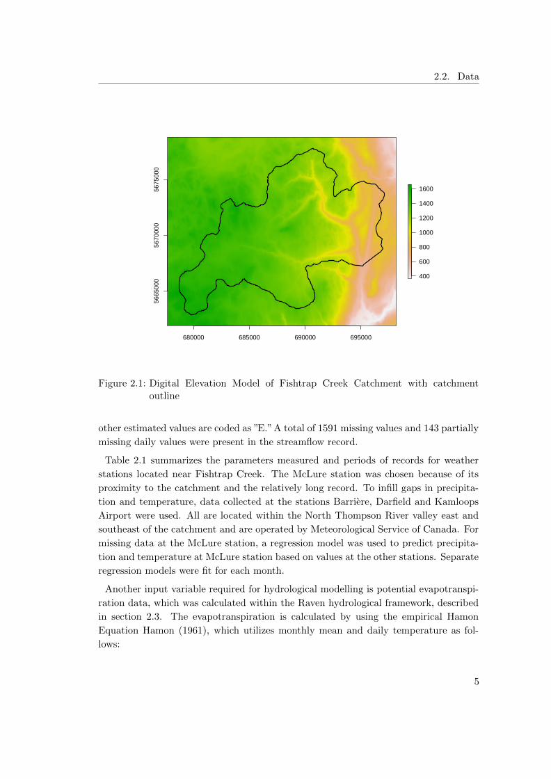
Land cover was represented as three different classes: forest, open and lake. Six aerial
photograph data sets from 1974, 1981, 1986, 1990, 1995 and 2000 were used to map
forest cover by M. Chuang (pers. comm.). Chuang distinguished three forest cover
types: fresh clearcut, young forest and old forest. In this study, the young forest and
old forest were grouped together.
Lakes were classified using shapefiles downloaded from the Atlas of Canada, an online
data base for multiple spatial data by Natural Resources Canada. Remaining areas,
not classified as forest or lake, were defined as open areas. By combining the three land
cover types, an area-wide continuous shape file was created.
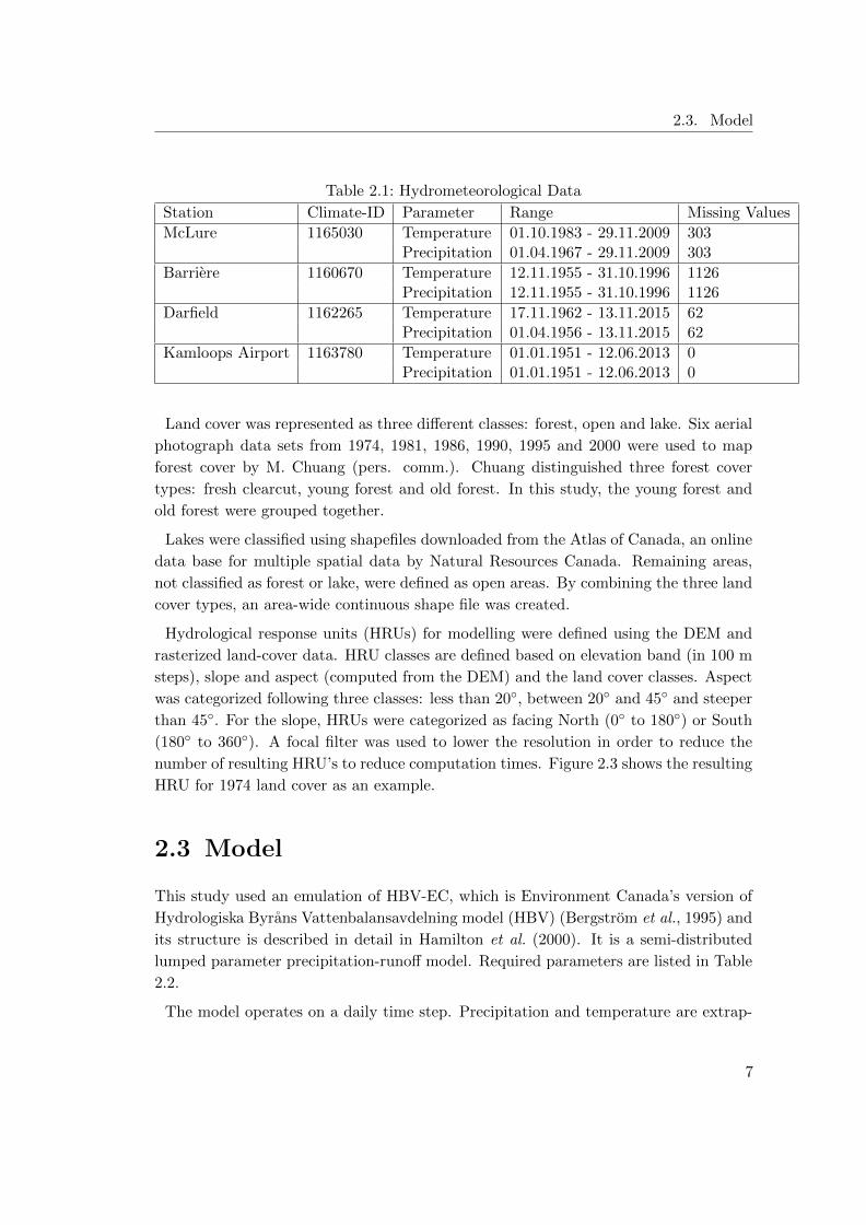
Hydrological response units (HRUs) for modelling were defined using the DEM and
rasterized land-cover data. HRU classes are defined based on elevation band (in 100 m
steps), slope and aspect (computed from the DEM) and the land cover classes. Aspect
was categorized following three classes: less than 20◦, between 20◦ and 45◦ and steeper
than 45◦. For the slope, HRUs were categorized as facing North (0◦ to 180◦) or South
(180◦ to 360◦). A focal filter was used to lower the resolution in order to reduce the
number of resulting HRU’s to reduce computation times. Figure 2.3 shows the resulting
HRU for 1974 land cover as an example.
2.3 Model
This study used an emulation of HBV-EC, which is Environment Canada’s version of
Hydrologiska Byrans Vattenbalansavdelning model (HBV) (Bergstrom et al., 1995) and
its structure is described in detail in Hamilton et al. (2000). It is a semi-distributed
lumped parameter precipitation-runoff model. Required parameters are listed in Table
2.2.
The model operates on a daily time step. Precipitation and temperature are extrap-
7
2.3. Model
Figure 2.3: Hydrologic Response Units;Exemplary result from processing spatial datausing 1974 land cover; Colors responding to a combined parameter valuederived from
olated from the weather station to the center of each HRU to include lapse rate effects.
The model accounts for interception loss from forest canopy, and simulates the accu-
mulation and melt of snow, including calculation of snowpack cold content and water
retention. Snow melt is computed using a temperature-index approach, with the melt
factor allowed to vary as a function of time of year, land cover, and slope-aspect. Rain
and/or meltwater are added to the soil moisture storage. The soil routine regulates
drainage based on the ratio of soil moisture to field capacity, and evapotranspiration is
a function potential evapotranspiration and the ratio of soil moisture to field capacity.
Drainage of water from the soil moisture storages for each HRU is routed through
lumped reservoirs. In the configuration used here, the model features two parallel
reservoirs. The fast reservoir, which can be nonlinear depending on the value of a
coefficient, represents fast flow paths such as overland flow and shallow subsurface flow,
8
2.3. Model
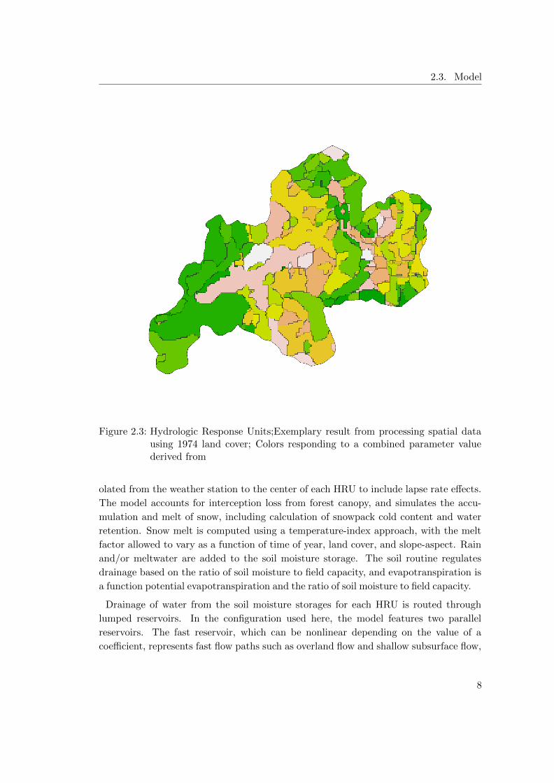
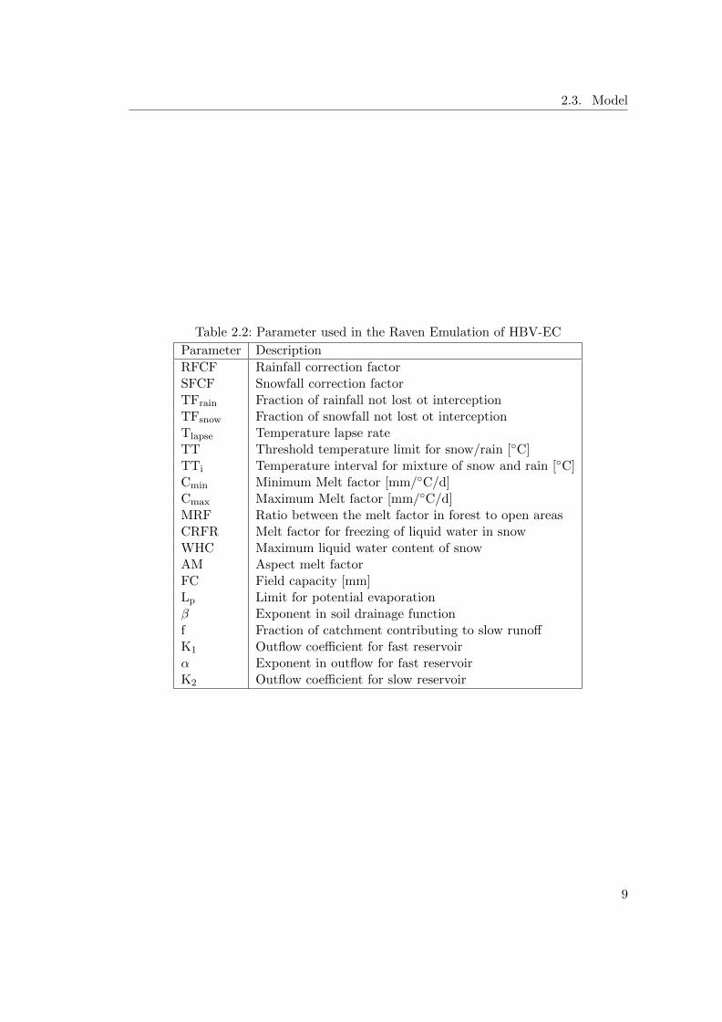
Table 2.2: Parameter used in the Raven Emulation of HBV-EC
Parameter Description
RFCF Rainfall correction factorSFCF Snowfall correction factorTFrain Fraction of rainfall not lost ot interceptionTFsnow Fraction of snowfall not lost ot interceptionTlapse Temperature lapse rateTT Threshold temperature limit for snow/rain [◦C]TTi Temperature interval for mixture of snow and rain [◦C]Cmin Minimum Melt factor [mm/◦C/d]Cmax Maximum Melt factor [mm/◦C/d]MRF Ratio between the melt factor in forest to open areasCRFR Melt factor for freezing of liquid water in snowWHC Maximum liquid water content of snowAM Aspect melt factorFC Field capacity [mm]Lp Limit for potential evaporationβ Exponent in soil drainage functionf Fraction of catchment contributing to slow runoffK1 Outflow coefficient for fast reservoirα Exponent in outflow for fast reservoirK2 Outflow coefficient for slow reservoir
9
2.4. Calibration and validation
while the slow reservoir conceptually represents baseflow associated with discharge of
deeper groundwater.
This study used an emulation of the HBV-EC model within the Raven modelling plat-
form Craig & the Raven development team (2016). The Raven platform has a flexible
structure that allows the user to build a model by choosing among a range of spatial
structures and process representations. Within Raven, model equations are framed as
differential equations that are solved using robust and fast numerical schemes.
2.4 Calibration and validation
In order to calibrate the model, two different approaches were used, Particle Swarm
Optimization (PSO) and Dynamically Dimensioned Search (DDS).
Particle Swarm Optimization (Kennedy & Eberhart, 1995) is a population based op-
timisation algorithm, which does not utilize selection like evolutionary algorithms. It
starts with a group of random parameters and searches optima by updating genera-
tions. It finds the best solution by adjusting the particles postion based on its own
and its companions’ position. The Dynamically Dimensioned Search Algorithm Tol-
son & Shoemaker (2007) is a search algorithm, which is designed for calibrations with
many parameters. It was demonstrated to be more efficient and more robust than
common evolutionary algorithms like SCE Duan et al. (1993) when using more than 10
parameters for watershed model calibration. DDS starts searching globally and then
transitions into a more local search towards the iteration limit defined by the user, by
dynamically reducing the number of dimensions in the neighborhood.
Both approaches were used to calibrate models using the six land cover data sets,
resulting in a model family of 12 calibrated models. The Nash-Sutcliffe Efficiency
(NSE, Nash & Sutcliffe (1970)) was used as an objective function for all calibrations.
The calibration procedures were executed within the Ostrich (Matott (2005) platform, a
multi algorithm and model independent optimization software application. To calibrate
the set-up Raven HBV-EC model, parameter ranges for all parameters were defined.
The objective function NSE was calculated by Raven and then evaluated by Ostrich to
determine model fit and select parameters for the next model run.
The calibration/validation procedure was based on a split sample approach, in which
the modelling period was split into a 2/3 calibration phase (1970 to 1992) and a 1/3
validation period (1992 to 2003).
10
2.5. Change detection
2.5 Change detection
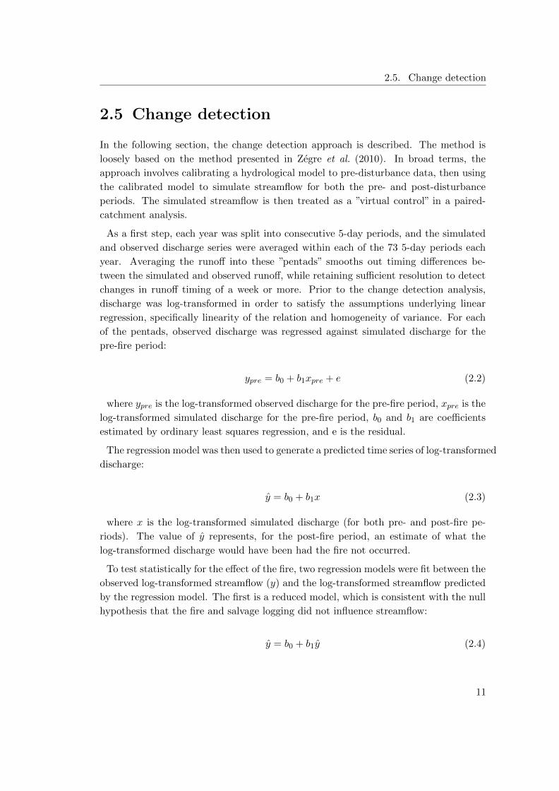
In the following section, the change detection approach is described. The method is
loosely based on the method presented in Zegre et al. (2010). In broad terms, the
approach involves calibrating a hydrological model to pre-disturbance data, then using
the calibrated model to simulate streamflow for both the pre- and post-disturbance
periods. The simulated streamflow is then treated as a ”virtual control” in a paired-
catchment analysis.
As a first step, each year was split into consecutive 5-day periods, and the simulated
and observed discharge series were averaged within each of the 73 5-day periods each
year. Averaging the runoff into these ”pentads” smooths out timing differences be-
tween the simulated and observed runoff, while retaining sufficient resolution to detect
changes in runoff timing of a week or more. Prior to the change detection analysis,
discharge was log-transformed in order to satisfy the assumptions underlying linear
regression, specifically linearity of the relation and homogeneity of variance. For each
of the pentads, observed discharge was regressed against simulated discharge for the
pre-fire period:
ypre = b0 + b1xpre + e (2.2)
where ypre is the log-transformed observed discharge for the pre-fire period, xpre is the
log-transformed simulated discharge for the pre-fire period, b0 and b1 are coefficients
estimated by ordinary least squares regression, and e is the residual.
The regression model was then used to generate a predicted time series of log-transformed
discharge:
y = b0 + b1x (2.3)
where x is the log-transformed simulated discharge (for both pre- and post-fire pe-
riods). The value of y represents, for the post-fire period, an estimate of what the
log-transformed discharge would have been had the fire not occurred.
To test statistically for the effect of the fire, two regression models were fit between the
observed log-transformed streamflow (y) and the log-transformed streamflow predicted
by the regression model. The first is a reduced model, which is consistent with the null
hypothesis that the fire and salvage logging did not influence streamflow:
y = b0 + b1y (2.4)
11
2.5. Change detection
The second, called the ”full” model, includes a categorical variable to distinguish the
pre-fire and post-fire periods. In terms of R syntax, the model can be expressed as
follows:
y ∼ y ∗ period (2.5)
where period is a categorical variable with two values, representing the two data
periods, and the product ”∗” indicates that all main effects of both variables and all
their interactions are included. An analysis of variance (ANOVA) is conducted to
compare the two models. If the p-value of the test is less than 0.05, then the full model
explains significantly more variance than the reduced model, and the null hypothesis
is rejected. The accepted hypothesis is that the fire and/or the salvage logging had a
statistically significant influence on discharge for a given pentad.
Following the change detection, both time series were back-transformed to compare
the discharge time series. To account for transformation bias, the discharge series were
corrected following Baskerville (1972). Differences between predicted and observed
post-fire discharge are then compared to assess the direction and magnitude of change
in the streamflow regime after the forest fire.
12
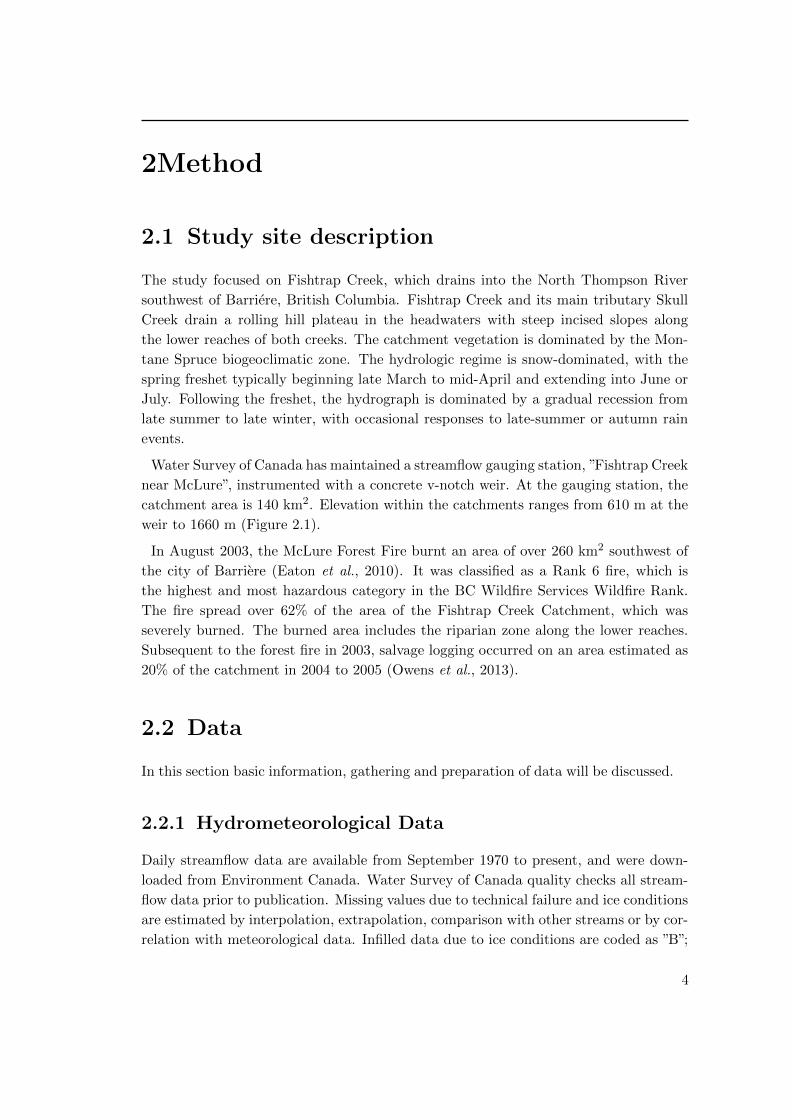
3Results
3.1 Overview of the studyperiod
In this section, a brief overview of the study period is given. The data presented here
was processed, as described in Section 2.2.
−30
−10
010
2030
Tem
pera
ture
[°C
]
05
1015
2025
Dis
char
ge [m
³/s]
5040
3020
100
Pre
cipi
tatio
n [m
m]
1972 1977 1982 1987 1992 1997 2002 2007
Figure 3.1: Timeseries of hydrometeorological data; the upper part of the figurepaneldisplays the daily temperature [◦C], Precipitation [mm] as blue bars andDischarge [m3s−1] as cyan line are shown in the lower part; the continuousvertical line marks the separation between calibration and validation whilethe dashed line shows the period of the forest fire.
13
3.1. Overview of the studyperiod
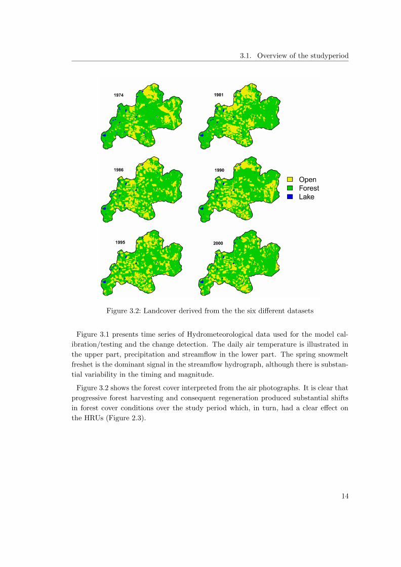
Figure 3.2: Landcover derived from the the six different datasets
Figure 3.1 presents time series of Hydrometeorological data used for the model cal-
ibration/testing and the change detection. The daily air temperature is illustrated in
the upper part, precipitation and streamflow in the lower part. The spring snowmelt
freshet is the dominant signal in the streamflow hydrograph, although there is substan-
tial variability in the timing and magnitude.
Figure 3.2 shows the forest cover interpreted from the air photographs. It is clear that
progressive forest harvesting and consequent regeneration produced substantial shifts
in forest cover conditions over the study period which, in turn, had a clear effect on
the HRUs (Figure 2.3).
14
3.2. Calibration and Testing
3.2 Calibration and Testing
In the following section, results of the model calibration are displayed.
Figure 3.3: Hydrograph comparison for the validation period; Each colour indicatesa different combination of optimization method and forest cover, and thedashed line is observed streamflow
Each of the 12 models resulting from the different calibration methods generated
Nash-Sutcliffe efficiencies in the range 0.74 to 0.82 for calibration and 0.77 to 0.89
for validation (Table 3.1). Fig. 3.3 compares validation-period hydrographs of all
calibrated models. The reduction to the calibration period is due to visual reasons. All
model families generated similar hydrographs, with the greatest variability associated
with autumn rain events. In general, most of these events were overpredicted, while
a minority of the events were reproduced to a sufficient level, e.g. the autumn event
in 2001 and 1995. All models matched the timing and shape of the freshet period
hydrograph, but underestimated streamflow in winter. The freshet was underpredicted
or matched for most of the years, and only in 2000 and 2001 did the majority of
the models generate a peakflow higher than the observed. The underestimation of
streamflow in winter is consistent throughout the calibration period for all models and
streamflow is declining constantly from the last rain event in autumn until the first
peak in spring caused by the freshet.
15
3.2. Calibration and Testing
Table 3.1: NSE values for calibration and validation periods
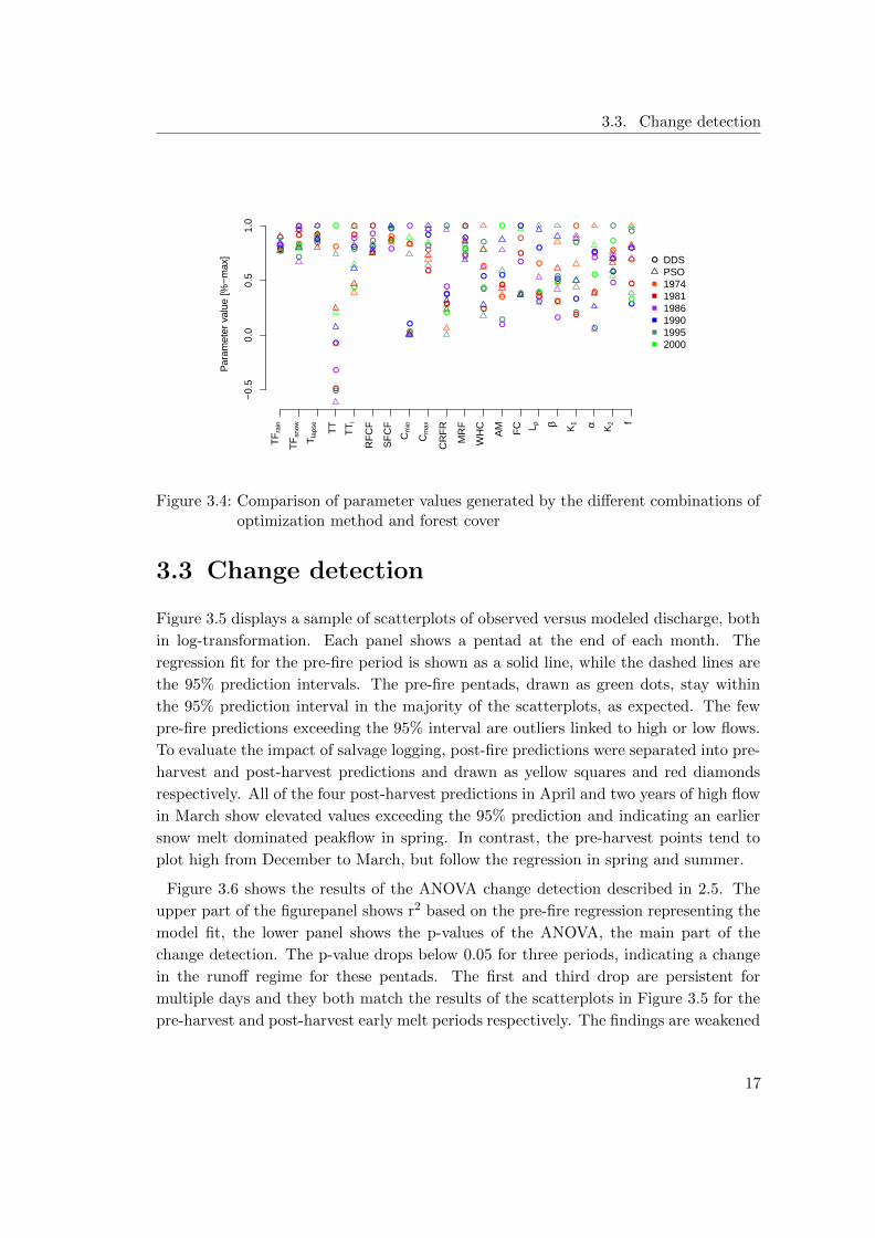
Figure 3.4 illustrates the variability of each parameter as a function of land cover and
calibration approach. To facilitate plotting on a single graph, the parameter estimates
were normalized as follows:
Pi∗ = Pi/max(Pi) (3.1)
where Pi represents the parameter estimate for a single combination of calibration
method and forest cover. With this scaling, a clustering of points near 1 indicates
little parameter variability, and an increasing range between 0 and 1 indicates higher
variability.
The parameters that influence precipitation – including the rainfall and snowfall cor-
rection factors (RFCF and SFCF ) and the throughfall fractions (TFrain and TFsnow)
– exhibit relatively little variability. Most of the other parameters exhibit substantial
variability, although it should be noted that the temperature thresholds for the rain-
snow transition (TT ) can take negative values, making the scaled values more difficult
to interpret. Some parameters tend to separate into clusters (e.g. Cmin and FC), while
no calibration method leads to a values in between those clusters. But overall, there
is no obvious separation based on the calibration method which would be either land
cover or algorithm related, which suggests that most of the parameter variability is
driven by the use of different forest covers to define HRUs.
16
3.3. Change detection
●●●●
●
●●
●●●
●
● ●
●●●
●
●
●
●
●
●
●
● ●
●●
●●
●
●
●
●
●●●
●●
●
●●
●
●
●
●
●
●●
●
●
●
●●
●
●
●
●
●
●
●
●
●
●
●
●●
●
●
●
●
●
●
●
●
●
●
●
●
●
●
●
●
●●
●
●●
●
●●
●
●
●
●●●
●
●
●
●
●
●
●
●●●
●
●
●
●
●
●
●
●
●
●
●
●
●
●
−0.
50.
00.
51.
0
Par
amet
er v
alue
[%−
max
]
TF
rain
TF
snow
Tla
pse
TT
TT
i
RF
CF
SF
CF
Cm
in
Cm
ax
CR
FR
MR
F
WH
C
AM FC L p β K1 α K2 f
● DDSPSO197419811986199019952000
Figure 3.4: Comparison of parameter values generated by the different combinations ofoptimization method and forest cover
3.3 Change detection
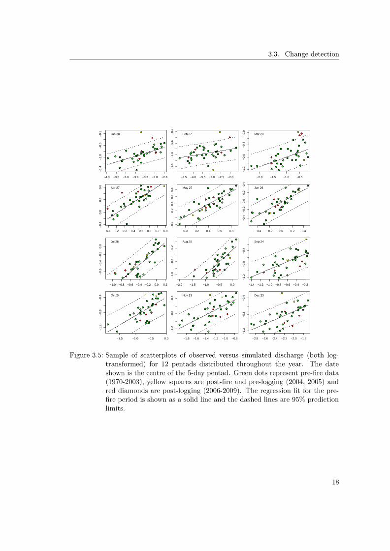
Figure 3.5 displays a sample of scatterplots of observed versus modeled discharge, both
in log-transformation. Each panel shows a pentad at the end of each month. The
regression fit for the pre-fire period is shown as a solid line, while the dashed lines are
the 95% prediction intervals. The pre-fire pentads, drawn as green dots, stay within
the 95% prediction interval in the majority of the scatterplots, as expected. The few
pre-fire predictions exceeding the 95% interval are outliers linked to high or low flows.
To evaluate the impact of salvage logging, post-fire predictions were separated into pre-
harvest and post-harvest predictions and drawn as yellow squares and red diamonds
respectively. All of the four post-harvest predictions in April and two years of high flow
in March show elevated values exceeding the 95% prediction and indicating an earlier
snow melt dominated peakflow in spring. In contrast, the pre-harvest points tend to
plot high from December to March, but follow the regression in spring and summer.
Figure 3.6 shows the results of the ANOVA change detection described in 2.5. The
upper part of the figurepanel shows r2 based on the pre-fire regression representing the
model fit, the lower panel shows the p-values of the ANOVA, the main part of the
change detection. The p-value drops below 0.05 for three periods, indicating a change
in the runoff regime for these pentads. The first and third drop are persistent for
multiple days and they both match the results of the scatterplots in Figure 3.5 for the
pre-harvest and post-harvest early melt periods respectively. The findings are weakened
17
3.3. Change detection
●
●
●
●
●
●
●
●
●
●
●
●
●●
●
●
●
●
●
●●
●
●
●
●
●
●
●●
●
●
−4.0 −3.8 −3.6 −3.4 −3.2 −3.0 −2.8
−1.
4−
1.0
−0.
6−
0.2
x
Jan 28
●●●
●
●
●
●
●
●●●
●
● ●●
●
●
●
● ●
●
●
●
●●
●
●●● ●
●
−4.5 −4.0 −3.5 −3.0 −2.5 −2.0
−1.
4−
1.0
−0.
6−
0.2
x
y
Feb 27
●●
●
●
●
●
●
●
●●
●
●
●
●
●
●
●
●
●
●
●
●
●
●●
●
●●
●●
●
−2.0 −1.5 −1.0 −0.5
−1.
2−
0.8
−0.
40.
0
x
y
Mar 28
●
●
●
●
●
●
●
●
●
●
●
●
●
●
●
●
●●
●●●
●
●
●
●●
●●
●
●
●
0.1 0.2 0.3 0.4 0.5 0.6 0.7 0.8
−0.
40.
00.
40.
8
x
Apr 27
●
●
●
●
●
●
●
●
●
●
●
●●
●
●●
●
●
●
●
●
●
●
●
●
●
●
●
●
●
●
0.0 0.2 0.4 0.6 0.8
−0.
20.
20.
40.
60.
8
x
y
May 27
●
●
●
●
●
●
●
●
●
●
●
●
●
●
●●
●
●
●
●
●
●
●
●●
●
●
●
●●
●
−0.4 −0.2 0.0 0.2 0.4
−0.
4−
0.2
0.0
0.2
0.4
xy
Jun 26
●
●●
●
● ●
●
●●
●
●●
●
●
●●
●
●
●
●
●
●
●
●
●
●
●
●
●
●
−1.0 −0.8 −0.6 −0.4 −0.2 0.0 0.2
−0.
6−
0.4
−0.
20.
0
x
Jul 26
●
●
●
●
●
●
●
●
●
●
●●
●
●
●
●
●
●
●
●
●
●
●
●●
●
●
●
●
●
−2.0 −1.5 −1.0 −0.5 0.0
−1.
0−
0.6
−0.
2
x
y
Aug 25
●●
●
●
●●
●
●
●
●
●● ●
●
●
●
●
●
●
●
●
●
●
●●
●
●●
●●
−1.4 −1.2 −1.0 −0.8 −0.6 −0.4 −0.2
−1.
2−
0.8
−0.
4
x
y
Sep 24
●
●
●
●
●
●
●
●
●●
●
●
●
●
●
●
●
●
●
●
●
●
●
●
●
●
●
●
●●
−1.5 −1.0 −0.5 0.0
−1.
2−
0.8
−0.
4 Oct 24
●●
●
●
●
●
●
●
●
●
●
●●
●
●
●
●
●
●
●●
●
●
●●
●
●
●
●
●
−1.8 −1.6 −1.4 −1.2 −1.0 −0.8
−1.
2−
0.8
−0.
4
y
Nov 23
●●
●
●
●
●
●
●
●
●●
● ●
●
●
●
●
●
● ●
●
●
●
●
●
●
●
●
●
●
−2.8 −2.6 −2.4 −2.2 −2.0 −1.8
−1.
2−
0.8
−0.
4
y
Dec 23
Figure 3.5: Sample of scatterplots of observed versus simulated discharge (both log-transformed) for 12 pentads distributed throughout the year. The dateshown is the centre of the 5-day pentad. Green dots represent pre-fire data(1970-2003), yellow squares are post-fire and pre-logging (2004, 2005) andred diamonds are post-logging (2006-2009). The regression fit for the pre-fire period is shown as a solid line and the dashed lines are 95% predictionlimits.
18
3.3. Change detection
by the low r2 in late February and late April, indicating a bad model fit during the
early melt period.0.
00.
40.
8
r pre
2
0.00
10.
050
1.00
0
Day of year
p(F
>F
calc)
0 50 100 150 200 250 300 350
Figure 3.6: Results of the ANOVA change detection; the upper part of the figurepanelshows R2 associated with the pre-fire regression; the lower part panel showsthe p-value of for the ANOVA
Figure 3.7 displays the pre-fire predictions and observed streamflow in the upper and
their difference in the lower panel. Both show the 95% prediction interval as a grey line.
The upper panel suggests that the predicted streamflow follows the observed stream-
flow and matches its timing while the observed streamflow does not exceed the 95%
prediction interval. The difference in models reveals the later prediction of peak flows in
1992 and 1997, while in other years peak flow is timed correctly but overpredicted (e.g.
1991,1993 and 2000). The difference does not exceed the 95% prediction interval.
Figure 3.8 presents the post-fire runoff, predicted streamflow and difference in the
same way as the pre-fire discharge in Figure 3.7. The post-harvest discharge shows
earlier peaks than the predicted runoff and an exceedance of 95% in 2006 and 2007.
The difference shows that there is not only an earlier melt, but also a longer period
of high flow. In the winter of 2004-2005 the observed runoff exceeded the prediction
interval beginning in December 2004 and showing two minor peaks in early 2005, while
the peak was overpredicted. In 2004 and 2008 relatively low peak flows occurred which
did not exceed the prediction interval.
19
3.3. Change detection
04
812
Q (
m3 s−1
)observed Q predicted Q 95% pred. limits
−2
02
4
Qob
s−
Qpr
ed (
m3 s−1
)
1991 1993 1995 1997 1999 2001 2003
Figure 3.7: Predicted and observed streamflow in the pre-fire period, with 95% predic-tion limits.
04
812
Q (
m3 s−1
) observed Q predicted Q 95% pred. limits
−2
02
4
Qob
s−
Qpr
ed (
m3 s−1
)
2004 2005 2006 2007 2008 2009
Figure 3.8: Predicted and observed streamflow in the post-fire period, with 95% pre-diction limits.
20
3.3. Change detection
As seen in Figure 3.5, the post-fire data tend to plot higher than the pre-fire data
in late winter and through April. This result is confirmed by the ANOVA (Figure
3.6), which indicates the effect of the fire was statistically significant for those periods
at a 5% significance level. Consistent with these results, Figure 3.8 shows that, in
many years, the spring freshet began earlier than predicted with predicted flow in April
sometimes exceeding the 95% prediction limit. Of particular note is 2005, in which it
appears that warm weather in late winter generated early rises in the hydrograph that
are not apparent in the pre-fire period. By contrast, observed streamflow generally
remained within the 95% prediction limits for the pre-fire period, with a less consistent
occurrence of observed flow exceeding predicted on the rising limb of the freshet (Figure
3.8).
21
4Discussion
This study demonstrated that many of the calibrated parameters in the HBV-EC model
are sensitive to which land cover from within the calibration period was used to set up
the model and define the HRUs. To the author’s knowledge, this source of uncertainty
has not been identified and quantified by previous research. Although time did not
allow an assessment of other sources of uncertainty in this study, it would be valuable
to extend the current study to quantify those other sources of uncertainty – model
structure, input data, and streamflow data – to provide a more complete understanding
of parameter uncertainty.
The finding that streamflow increases appeared to be confined to late winter and spring
is broadly consistent with the results of Eaton et al. (2010), who used a purely statistical
approach. They found an increase in annual runoff and a strong increase in April, but
no apparent change in peak flow. Eaton et al. (2010) hypothesized that the fire and
salvage harvesting desynchronized snowmelt runoff between disturbed and undisturbed
portions, such that snow in disturbed areas began melting earlier, and made less of
a contribution during May and early June, when most pre-fire peak flows occurred.
The results of this thesis provide further support for this hypothesis by showing that,
from May onward, there was no detectable increase in 5-day averaged streamflow. The
change detection approach applied in this study was successful in detecting periods of
increased streamflow in late winter and spring. However, the power of the test was
likely limited by the relatively weak pre-harvest regressions, especially in winter, and it
must be remembered that an inability to detect a change does not mean that a change
did not occur. The lack of power was caused by an inability of the calibrated model
to reproduce with high accuracy the interannual variations in streamflow. This was
especially the case in winter, when r2 dropped to about 0.5.
The changes of streamflow within the pre-harvesting, which differ from the changes in
the post-harvesting period might be linked to different reasons. The different findings
of effects of forest fire on soil hydrophobicity (Letey, 2001; Bento-Goncalves et al., 2012)
makes these changes hard to interpret. They can be also linked to the high temperature
during the early winter of 2005.
Some of this uncertainty is likely associated with extrapolating precipitation data
from a valley bottom location to the higher elevations on the plateau, which dominate
the hydrology of Fishtrap Creek. However, some of the error is likely associated with
model structure – in particular, inability to reproduce winter baseflow. It would be
interesting to repeat this study using a different model, structured so as to reproduce
winter baseflow more accurately. Another avenue for potentially improving the model
22
would be to use additional information to assist in calibration. For example, the Min-
istry of Forests, Lands and Natural Resource Operations has monitored snowpack water
equivalent at disturbed and undisturbed sites just outside the Fishtrap Creek catch-
ment (Winkler et al., 2005), and these could be used to help calibrate the parameters
governing snow accumulation and ablation.
23
5Conclusions
5.1 Summary of key findings
5.1.1 Calibration
The HBV-EC model calibration using the DDS and PSO optimization algorithms with
six different land cover data sets resulted in a model family of 12 models. All of
them produced discharge of a similar regime, with minor differences in total volume.
Neither the land cover data set nor the calibration algorithm had a major effect on
daily discharge simulations. All combinations of land cover and optimization algorithm
tended to underestimate winter stream flows, likely because the model structure did
not represent the aquifer structure correctly. All calibrations accurately reproduced the
timing of the spring snow melt peak flow response, but underestimated the volume.
This analysis indicates that specification of land cover can be a significant source
of parameter uncertainty, in addition to the effects of uncertainties in meterological
and streamflow and model structure, which have been the subject of previous research
(e.g.,Beven (1993); Beven & Freer (2001)).
5.1.2 Change detection
The change detection method applied in this thesis successfully detected change in
the runoff regime of Fishtrap Creek after the McLure Forest Fire. The key changes
included an earlier onset of the spring freshet in many years, and statistically significant
higher streamflow between mid-March and early June. Streamflow changes were more
consistent in the years following extensive salvage logging. The lack of a significant
change in streamflow in late winter may reflect a lack of statistical power due to the
weaker pre-fire regressions for that period.
The model-based change detection method developed and applied in this study is
capable of detecting change in forest fire affected catchments, and shows promise as an
effective tool for medium to large scale catchments for which effective control catch-
ments are generally not available. The main challenge in applying the method is the
need for long and complete records of air temperature and precipitation from a single
weather station with a homogeneous record.
24
5.2. Recommendations for further research
5.2 Recommendations for further research
The model-based change detection approach should be tested with different calibration
methods to explore further the magnitude of this source of uncertainty. In addition,
applying the approach with different model structures might improve its performance
by allowing a better fit to the pre-disturbance streamflow data.
Another avenue for further research would be to use a process-based model to sim-
ulate directly the effects of the disturbance by modifying the land cover and HRUs
to represent disturbed conditions. It would be interesting to compare simulations for
a disturbed land-cover scenario to those for a control scenario, with pre-disturbance
land cover to assess whether the model can reproduce the observed post-disturbance
streamflow.
25
Bibliography
Baskerville, GL. 1972. Use of logarithmic regression in the estimation of plant biomass.
Canadian Journal of Forest Research, 2(1), 49–53.
Bates, Carlos G. 1921. First results in the streamflow experiment, Wagon Wheel Gap,