MIMAP TECHNICAL PAPER SERIES NO. 5 Profile of Poverty in Pakistan, 1998-99 SARFRAZ K. QURESHI Former Director and G. M. ARIF Senior Research Demographer January 2001 PAKISTAN INSTITUTE OF DEVELOPMENT ECONOMICS ISLAMABAD, PAKISTAN
Transcript
MIMAP TECHNICAL PAPER SERIES NO. 5
Profile of Poverty in Pakistan, 1998-99
SARFRAZ K. QURESHI
Former Director
and
G. M. ARIF Senior Research Demographer
January 2001
PAKISTAN INSTITUTE OF DEVELOPMENT ECONOMICS ISLAMABAD, PAKISTAN
ii
This Work is carried out with the financial assistance from the International Development Research Centre, Ottawa, Canada.
MIMAP Technical Paper Series No. 5 This study is a component of the Micro Impact of Macroeconomic Adjustment Policies (MIMAP) Pakistan project. This project is being implemented by the Pakistan Institute of Development Economics, Islamabad. The main aim of this project is to analyse the impact of structural adjustment policies on income distribution and poverty in Pakistan.
ISBN 969-461-101-6
Pakistan Institute of Development Economics Quaid-i-Azam University Campus, P O Box No. 1091 Islamabad 44000, Pakistan. Tel: 92-51-9206610-27 Fax: 91-51-9210886 E-mail: [email protected] The Pakistan Institute of Development Economics, established by the Government of Pakistan in 1957, is an autonomous research organisation devoted to carrying out theoretical and empirical research on development economics in general and on Pakistan-related economic issues in particular. Besides providing a firm foundation on which economic policy-making can be based, its research also provides a window through which the outside world can see the direction in which economic research in Pakistan is moving. The Institute also provides in-service training in economic analysis, research methods, and project evaluation.
CONTENTS
Page 1. Introduction 1
2. Data Sources and Determination of Poverty Lines 2
Data Sources 2 Determination of Poverty Lines 4 3. Calorie Intake (Per Capita) and Consumption Expenditure 7 4. Incidence of Poverty in 1998-99 8 5. Trends in Poverty 9 6. Decomposition of Poverty Across Socio-economic Groups 12 7. Determinants of Poverty 15 8. Conclusion 17
Appendices 19 References 20
List of Tables
Table 1. Poverty Lines (Per Capita) Based on Calorie Intake and Basic Need Approaches by Rural and Urban Areas 6
Table 2. Per Capita Calorie Intake by Province and Rural/Urban Area 7 Table 3. Distribution of Monthly Household Consumption Expenditure 8 Table 4. Proportion of Poor Household (Head-count Ratios) by Rural and
Urban Areas, 1998-99 9 Table 5. Trends in the Incidence of Poverty (Head-count Ratios) 10 Table 6. Trends in Food Poverty, 1984-85 – 1998-99 11 Table 7. Incidence of Poverty (Head-count Ratios) under the Basic Needs
Approach by Rural/Urban Area 12 Table 8. Incidence of Food Poverty (Head-count Ratios) by Farm Status of
Rural Households 13 Table 9. Decomposition of Poverty Across Socio-economic Groups, 1998-
99 14 Table 10. Logistic Regression Effects of Predictors on Being Poor (Odds
Ratios) 16
4
4
Appendix Table 1. Distribution of the Sample PSUs and SSUs with their Urban/Rural and Provincial Break-down, 1998-99 PSES and 1987-88 HIES 19
Appendix Table 2. Calorie Requirement by Age and Sex 19
1. INTRODUCTION
A number of studies have been undertaken during the last three decades to assess
the extent and nature of poverty in Pakistan. These studies are primarily based on data
generated by the Household Income and Expenditure Surveys (HIES), the earliest
relating to 1963-64. Most of the studies have used the calorie-intake approach to
assessing poverty, although a few recent studies have also used the basic-needs approach
to determine the level of poverty.1 There is a consensus among the studies that in the
1960s, rural poverty increased while urban poverty decreased. In the following decade,
poverty declined at all levels. This declining trend continued until 1987-88. Since then no
real consensus emerged on the trends in poverty. Gazdar et al. (1994) and Jafri (1999),
for example, show that decline in poverty continued in the early 1990s. Malik (1992);
Amjad and Kemal (1997) and Ali and Tahir (1999), on the other hand, show an increase
in poverty during this period.
No information on the incidence of poverty is available after the period of 1993-94.
The last HIES, the common source of measuring poverty in Pakistan, was conducted in
1996-97. It has only recently been released and estimates of poverty based on this data set
are not yet available. The HIES results are usually made available with a time lag of 2-3
years, leading to ineffective monitoring of trends in poverty. This necessitated the
conduct of a survey to measure the incidence of poverty for more recent period and also
to compare it with the earlier estimates.
The Pakistan Institute of Development Economics (PIDE) designed a research
project entitled “Micro Impacts of Macroeconomic Adjustment Policies (MIMAP)” to
examine the impact of structural adjustment program on the poor and vulnerable groups
1 See, for example, Ahmed (1993); Jafri and Khattak (1995); Jafri (1999).
6
6
of the society. This project carried out a household survey between March and July 1999,
with the aim to generate nationally representative data to examine the incidence of
poverty and distribution of income. The present study has used this survey data to
determine the level of poverty for the period of 1998-99 based on two approaches: calorie
intake and basic needs.
The previous studies have decomposed poverty across different socio-economic
groups, but farm status of households has seldom been included in the analyses. This
variable could be closely associated with poverty in rural areas. The present study while
decomposing poverty across different socio-economic groups has included this variable
in the analysis. The determinants of poverty based on logistic regressions have also been
estimated. It is determined that policy-influenced variables such as schooling and
employment creation are important factors that can lead to a significant reduction in
poverty levels.
Data sources and methodology are discussed in Section 2, followed by discussion
on calorie intake and consumption expenditure in Section 3. Incidence and trends in
poverty are reported in Sections 4 and 5. The subsequent section provides data on
decomposition of poverty across different socio-economic groups. Determinants of
poverty are reported in Section 7, followed by conclusion in the final section.
2. DATA SOURCES AND DETERMINATION OF POVERTY LINES
Data Sources
The main data source used in this study is the household survey carried out by the
MIMAP project of the PIDE named as ‘the 1998-99 Pakistan Socio-economic Survey’
(PSES)2. The universe of the PSES consists of all urban and rural areas of the four
provinces of Pakistan as defined by the 1981 population census excluding FATA,
restricted military areas, districts of Kohistan, Chitral, Malakand, and protected areas of
2For comparison, this study has also used extensively the 1993-94 HIES data set. The sample design
of this data set is discussed in the respective report [Pakistan (1996)].
7
7
NWFP. The population of the excluded areas constitutes about 4 percent of the total
population. The village list published by the population census organisation in 1981 was
taken as sampling frame for drawing the sample for rural areas. For urban areas, sampling
frame developed by the Federal Bureau of Statistics (FBS) was used.
Two stage stratified sample design was adopted for the 1998-99 PSES.
Enumeration blocks in urban domain and Mouzas/dehs/villages in rural domain were
taken as primary sampling units (PSUs). Households within the sampled PSUs were
taken as secondary sampling units (SSUs). Within a PSU, a sample of 8 households from
urban domain and 12 households from rural domain was selected.
The main objective of the MIMAP project was to examine the impact of structural
adjustment programme on poor and vulnerable groups of the society. In order to conduct
such an analysis, the 1998-99 PSES was carried out in those PSUs that were covered in
the second quarter of the 1987-88 HIES, the last survey carried out before the
commencement of adjustment programme in 1989. By selecting those PSUs that were
covered in the pre-adjustment period, with and without analysis would be possible.3
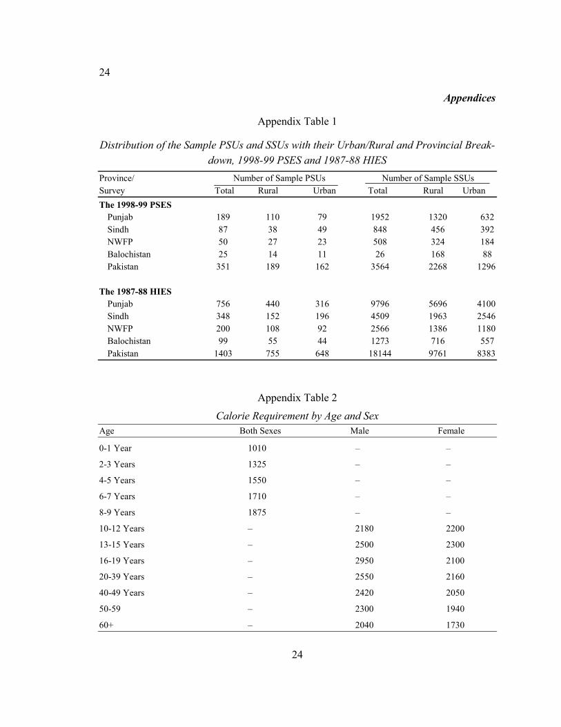
Distribution of the 1998-99 PSES sample by province and rural/urban is reported in
Appendix Table 1. The sample of the 1987-88 HIES is also shown in this Table. The
entire sample of the 1987-88 HIES was drawn during the whole year from 1403 PSUs
(755 rural and 648 urban). These PSUs were grouped into four equal parts and one group
of 351 PSUs was enumerated in one quarter. The 1998-99 PSES was carried out in those
351 PSUs that were covered during the second quarter of the 1987-88 HIES. Appendix
Table 1 shows that sampled households covered during the 1998-99 PSES numbered
3564 (2268 rural and 1296 urban).
The data generated by the 1998-99 PSES is representative at the national level as
well as for rural and urban areas of the country (for more detail on the sample design of
the PSES, see Arif et al. (2001). However, there is a need to clarify couple of points. As
3However this analysis has not been carried out in this paper. It will be dealt in a separate paper.
8
8
mentioned earlier that the entire sample of the PSES was drawn from those PSUs that
were covered during the 1987-88 HIES. In 1987-88 the entire country was divided by the
FBS into 18000 PSUs. In the 1990s this number has increased to 23000. Whether this
change in the total number of PSUs has affected the representativeness of the PSES
sample. The change however has not affected it for two reasons. First, the numbers of
PSUs were primarily increased in urban areas. In other words, the change in rural domain
was minimal. Second, even in urban domain, because of increase in number of dwellings
in some PSUs or reclassification of urban areas, the boundaries of old PSUs were
changed in such a way that on average each PSU consisted of 200 to 250 households.
Only few entirely new PSUs have been added. These adjustments in the sampling frame
are not likely to have affected the representativeness of the PSES sample.
As noted above, the HIES sample is drawn during the whole year from the selected
PSUs. It thus takes care of the seasonal variations. The 1998-99 PSES was completed in
only four months, March–June, 1999. Apparently it did not take care of the seasonal
variations. These variations are not likely to have affected the major part of the data set
generated by the PSES. They, however, may have influenced some variables such as
employment and health. Seasonal unemployment is particularly induced by fluctuations in
the demand for labour. The demand for agricultural employees declines after the planting
season and remains low until the harvest season. The PSES was carried out at the time of
wheat harvesting in most part of the country and cotton sowing in Punjab and Sindh
provinces. The demand for agricultural workers in rural areas could be high when the
survey was carried out, resulting a relatively lower level of unemployment [Nasir (2001)].
The seasonal variations may also affect the incidence of certain diseases; for
example, diarrhoeal morbidity in the rainy season as compared with the other seasons is
usually higher [Arif and Ibrahim (1998)]. While the 1998 PSES sample was not drawn
during the whole year, the incidence of those diseases that are likely to be affected by the
seasonal variations may not be representative for the survey year.
9
9
Determination of Poverty Lines
A poverty measure needs three elements: an indicator of well-being or welfare (e.g.
per capita calorie intake; per capita expenditure); a normative threshold representing the
well-being an individual (or household) must attain to be above poverty (e.g. a poverty
line); and an aggregate measure to assess poverty across population (e.g. head count
ratio). Poverty lines are generally drawn in absolute and/or in relative terms. Relative
poverty refers to the position of an individual or household compared with the average
income in the country. Absolute poverty refers to the position of an individual or a
household in relation to a specific poverty line. This study is based on absolute poverty
line. Two main methods are employed to compute the poverty line, the food energy
intake (FEI) method and the cost of basic needs (CBN) method.
The FEI method has been used to estimate the food poverty. It is argued that in
developing countries, such as Pakistan, where food constitutes a large share of the budget,
and where the concern with poverty is closely associated with under-nutrition, it makes sense
to use food and nutritional requirements to derive a poverty line. The construction of a
poverty line always involves arbitrariness [Deaton (1997)]. This study has determined
poverty lines based on the estimated cost of food consistent with a calorie intake of 2550 per
adult equivalent per day for rural areas. A daily intake of 2295 calories per adult equivalent is
considered for urban areas of the country.
The recommended level of calorie intake was converted into the following
functional form, as suggested by Ercelawn (1990):
C = a + b ln E
where C is a daily calorie-intake per adult equivalent and E is the monthly food expenditure per adult equivalent. Equivalence scale used in the study is reported in Appendix Table 2. Separate poverty lines were constructed for rural and urban areas. While constructing the poverty lines, data were cleaned up for outliers: households which had a food share below 5 percent and greater than 90 percent of total consumption, as
10
10
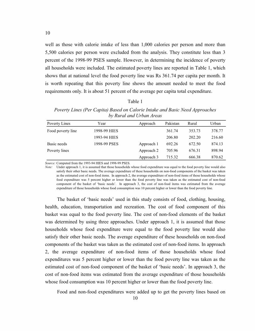
well as those with calorie intake of less than 1,000 calories per person and more than 5,500 calories per person were excluded from the analysis. They constitute less than 3 percent of the 1998-99 PSES sample. However, in determining the incidence of poverty all households were included. The estimated poverty lines are reported in Table 1, which shows that at national level the food poverty line was Rs 361.74 per capita per month. It is worth repeating that this poverty line shows the amount needed to meet the food requirements only. It is about 51 percent of the average per capita total expenditure.
Table 1
Poverty Lines (Per Capita) Based on Calorie Intake and Basic Need Approaches by Rural and Urban Areas
Source: Computed from the 1993-94 HIES and 1998-99 PSES. Note: Under approach 1, it is assumed that those households whose food expenditure was equal to the food poverty line would also
satisfy their other basic needs. The average expenditure of these households on non-food components of the basket was taken as the estimated cost of non-food items. In approach 2, the average expenditure of non-food items of those households whose food expenditure was 5 percent higher or lower than the food poverty line was taken as the estimated cost of non-food component of the basket of ‘basic needs’. In approach 3, the cost of non-food items was estimated from the average expenditure of those households whose food consumption was 10 percent higher or lower than the food poverty line.
The basket of ‘basic needs’ used in this study consists of food, clothing, housing, health, education, transportation and recreation. The cost of food component of this basket was equal to the food poverty line. The cost of non-food elements of the basket was determined by using three approaches. Under approach 1, it is assumed that those households whose food expenditure were equal to the food poverty line would also satisfy their other basic needs. The average expenditure of these households on non-food components of the basket was taken as the estimated cost of non-food items. In approach 2, the average expenditure of non-food items of those households whose food expenditures was 5 percent higher or lower than the food poverty line was taken as the estimated cost of non-food component of the basket of ‘basic needs’. In approach 3, the cost of non-food items was estimated from the average expenditure of those households whose food consumption was 10 percent higher or lower than the food poverty line.
Food and non-food expenditures were added up to get the poverty lines based on
11
11
basic needs approach. Separate lines were computed for rural and urban areas. These lines are reported under the three above discussed approaches in Table 1. Differences in the poverty lines (FEI and CBN) are large. On average the poverty line based on the basic needs approach 1 was 1.9 times the food poverty line. In the case of urban areas it increased to 2.3 times the food poverty line, reflecting high cost of living in urban areas of the country.
3. CALORIE INTAKE (PER CAPITA) AND CONSUMPTION EXPENDITURE
Since the poverty lines used in this study are based on daily calorie intake and
expenditure on food and non-food items, it seems necessary to look at data on calorie
intake and expenditure on food and non-food items. This data, based on the 1998-99 PSES,
has been presented in Tables 2 and 3. The PSES provides information on quantities of
different food items consumed by the sampled households during the month preceding the
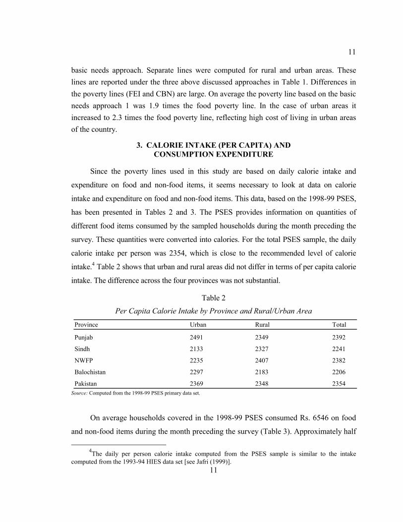
survey. These quantities were converted into calories. For the total PSES sample, the daily
calorie intake per person was 2354, which is close to the recommended level of calorie
intake.4 Table 2 shows that urban and rural areas did not differ in terms of per capita calorie
intake. The difference across the four provinces was not substantial.
Table 2
Per Capita Calorie Intake by Province and Rural/Urban Area
Province Urban Rural Total
Punjab 2491 2349 2392
Sindh 2133 2327 2241
NWFP 2235 2407 2382
Balochistan 2297 2183 2206
Pakistan 2369 2348 2354 Source: Computed from the 1998-99 PSES primary data set.
On average households covered in the 1998-99 PSES consumed Rs. 6546 on food
and non-food items during the month preceding the survey (Table 3). Approximately half
4The daily per person calorie intake computed from the PSES sample is similar to the intake computed from the 1993-94 HIES data set [see Jafri (1999)].
12
12
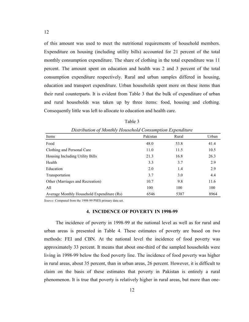
of this amount was used to meet the nutritional requirements of household members.
Expenditure on housing (including utility bills) accounted for 21 percent of the total
monthly consumption expenditure. The share of clothing in the total expenditure was 11
percent. The amount spent on education and health was 2 and 3 percent of the total
consumption expenditure respectively. Rural and urban samples differed in housing,
education and transport expenditure. Urban households spent more on these items than
their rural counterparts. It is evident from Table 3 that the bulk of expenditure of urban
and rural households was taken up by three items: food, housing and clothing.
Consequently little was left to allocate to education and health care.
Table 3
Distribution of Monthly Household Consumption Expenditure Items Pakistan Rural Urban
Food 48.0 53.8 41.4 Clothing and Personal Care 11.0 11.5 10.5 Housing Including Utility Bills 21.3 16.8 26.3 Health 3.3 3.7 2.9 Education 2.0 1.4 2.9 Transportation 3.7 3.0 4.4 Other (Marriages and Recreation) 10.7 9.8 11.6 All 100 100 100 Average Monthly Household Expenditure (Rs) 6546 5387 8964
Source: Computed from the 1998-99 PSES primary data set.
4. INCIDENCE OF POVERTY IN 1998-99
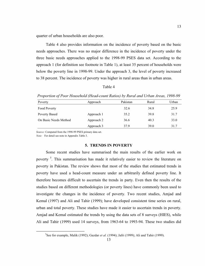
The incidence of poverty in 1998-99 at the national level as well as for rural and
urban areas is presented in Table 4. These estimates of poverty are based on two
methods: FEI and CBN. At the national level the incidence of food poverty was
approximately 33 percent. It means that about one-third of the sampled households were
living in 1998-99 below the food poverty line. The incidence of food poverty was higher
in rural areas, about 35 percent, than in urban areas, 26 percent. However, it is difficult to
claim on the basis of these estimates that poverty in Pakistan is entirely a rural
phenomenon. It is true that poverty is relatively higher in rural areas, but more than one-
13
13
quarter of urban households are also poor.
Table 4 also provides information on the incidence of poverty based on the basic
needs approaches. There was no major difference in the incidence of poverty under the
three basic needs approaches applied to the 1998-99 PSES data set. According to the
approach 1 (for definition see footnote in Table 1), at least 35 percent of households were
below the poverty line in 1998-99. Under the approach 3, the level of poverty increased
to 38 percent. The incidence of poverty was higher in rural areas than in urban areas.
Table 4
Proportion of Poor Household (Head-count Ratios) by Rural and Urban Areas, 1998-99 Poverty Approach Pakistan Rural Urban
Food Poverty 32.6 34.8 25.9
Poverty Based Approach 1 35.2 39.8 31.7
On Basic Needs Method Approach 2 36.6 40.3 33.0
Approach 3 37.9 39.0 31.7
Source: Computed from the 1998-99 PSES primary data set. Note: For detail see note in Appendix Table 3.
5. TRENDS IN POVERTY
Some recent studies have summarised the main results of the earlier work on
poverty 5. This summarisation has made it relatively easier to review the literature on
poverty in Pakistan. The review shows that most of the studies that estimated trends in
poverty have used a head-count measure under an arbitrarily defined poverty line. It
therefore becomes difficult to ascertain the trends in party. Even then the results of the
studies based on different methodologies (or poverty lines) have commonly been used to
investigate the changes in the incidence of poverty. Two recent studies, Amjad and
Kemal (1997) and Ali and Tahir (1999); have developed consistent time series on rural,
urban and total poverty. These studies have made it easier to ascertain trends in poverty.
Amjad and Kemal estimated the trends by using the data sets of 8 surveys (HIES), while
Ali and Tahir (1999) used 14 surveys, from 1963-64 to 1993-94. These two studies did
5See for example, Malik (1992); Gazdar et al. (1994); Jafri (1999); Ali and Tahir (1999).
14
14
not define a new poverty threshold. Rather they used the income poverty line defined by
Malik (1988) as a bench mark and adjusted it according to inflation.
Interestingly, for the period of 1963-64–1987-88, results of these two studies are
similar to the outcomes of previous studies based on different methodologies and poverty
lines. For this period, three main conclusions are usually drawn. First, poverty levels
increased between 1963-64 and 1969-70 overall as well as in rural areas, while it declined
in urban areas. Second, the next decade, 1969-70–1979, witnessed a decline in poverty in
both rural and urban areas. Third, this declining trend in poverty continued till 1987-88.
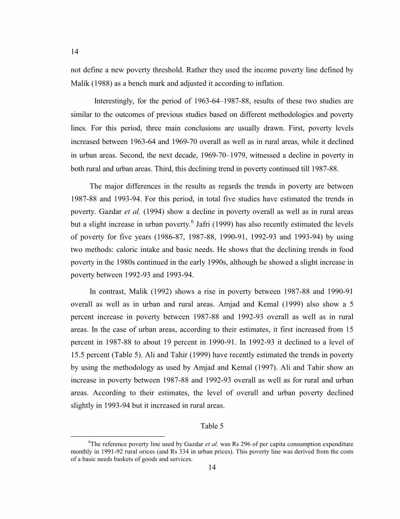
The major differences in the results as regards the trends in poverty are between 1987-88 and 1993-94. For this period, in total five studies have estimated the trends in poverty. Gazdar et al. (1994) show a decline in poverty overall as well as in rural areas but a slight increase in urban poverty.6 Jafri (1999) has also recently estimated the levels of poverty for five years (1986-87, 1987-88, 1990-91, 1992-93 and 1993-94) by using two methods: caloric intake and basic needs. He shows that the declining trends in food poverty in the 1980s continued in the early 1990s, although he showed a slight increase in poverty between 1992-93 and 1993-94.
In contrast, Malik (1992) shows a rise in poverty between 1987-88 and 1990-91 overall as well as in urban and rural areas. Amjad and Kemal (1999) also show a 5 percent increase in poverty between 1987-88 and 1992-93 overall as well as in rural areas. In the case of urban areas, according to their estimates, it first increased from 15 percent in 1987-88 to about 19 percent in 1990-91. In 1992-93 it declined to a level of 15.5 percent (Table 5). Ali and Tahir (1999) have recently estimated the trends in poverty by using the methodology as used by Amjad and Kemal (1997). Ali and Tahir show an increase in poverty between 1987-88 and 1992-93 overall as well as for rural and urban areas. According to their estimates, the level of overall and urban poverty declined slightly in 1993-94 but it increased in rural areas.
Table 5
6The reference poverty line used by Gazdar et al. was Rs 296 of per capita consumption expenditure monthly in 1991-92 rural orices (and Rs 334 in urban prices). This poverty line was derived from the costs of a basic needs baskets of goods and services.
15
15
Trends in the Incidence of Poverty (Head-count Ratios) Year Total Rural Urban
7The difference in the level of poverty between the two studies could largely be due to the procedure
adopted by Jafri to fill the missing data. This filling has probably increased the household consumption expenditure resulting in relatively lower estimates of poverty.
16
16
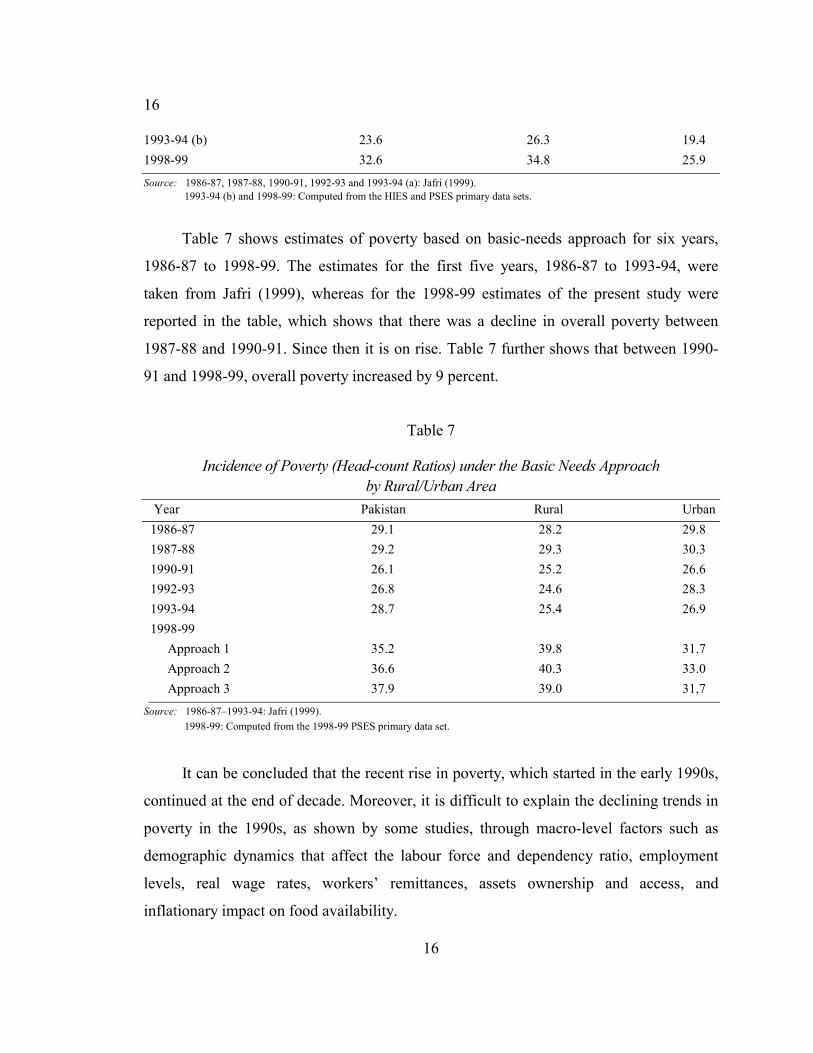
1993-94 (b) 23.6 26.3 19.4 1998-99 32.6 34.8 25.9
Source: 1986-87, 1987-88, 1990-91, 1992-93 and 1993-94 (a): Jafri (1999). 1993-94 (b) and 1998-99: Computed from the HIES and PSES primary data sets.
Table 7 shows estimates of poverty based on basic-needs approach for six years,
1986-87 to 1998-99. The estimates for the first five years, 1986-87 to 1993-94, were
taken from Jafri (1999), whereas for the 1998-99 estimates of the present study were
reported in the table, which shows that there was a decline in overall poverty between
1987-88 and 1990-91. Since then it is on rise. Table 7 further shows that between 1990-
91 and 1998-99, overall poverty increased by 9 percent.
Table 7
Incidence of Poverty (Head-count Ratios) under the Basic Needs Approach by Rural/Urban Area
Source: 1986-87–1993-94: Jafri (1999). 1998-99: Computed from the 1998-99 PSES primary data set.
It can be concluded that the recent rise in poverty, which started in the early 1990s,
continued at the end of decade. Moreover, it is difficult to explain the declining trends in
poverty in the 1990s, as shown by some studies, through macro-level factors such as
demographic dynamics that affect the labour force and dependency ratio, employment
levels, real wage rates, workers’ remittances, assets ownership and access, and
inflationary impact on food availability.
17
17
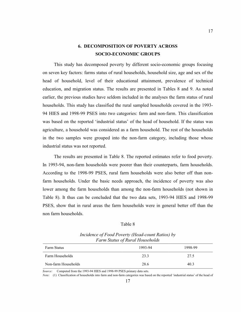
6. DECOMPOSITION OF POVERTY ACROSS SOCIO-ECONOMIC GROUPS
This study has decomposed poverty by different socio-economic groups focusing
on seven key factors: farms status of rural households, household size, age and sex of the
head of household, level of their educational attainment, prevalence of technical
education, and migration status. The results are presented in Tables 8 and 9. As noted
earlier, the previous studies have seldom included in the analyses the farm status of rural
households. This study has classified the rural sampled households covered in the 1993-
94 HIES and 1998-99 PSES into two categories: farm and non-farm. This classification
was based on the reported ‘industrial status’ of the head of household. If the status was
agriculture, a household was considered as a farm household. The rest of the households
in the two samples were grouped into the non-farm category, including those whose
industrial status was not reported.
The results are presented in Table 8. The reported estimates refer to food poverty.
In 1993-94, non-farm households were poorer than their counterparts, farm households.
According to the 1998-99 PSES, rural farm households were also better off than non-
farm households. Under the basic needs approach, the incidence of poverty was also
lower among the farm households than among the non-farm households (not shown in
Table 8). It thus can be concluded that the two data sets, 1993-94 HIES and 1998-99
PSES, show that in rural areas the farm households were in general better off than the
non farm households.
Table 8
Incidence of Food Poverty (Head-count Ratios) by Farm Status of Rural Households
Farm Status 1993-94 1998-99
Farm Households 23.3 27.5
Non-farm Households 28.6 40.3
Source: Computed from the 1993-94 HIES and 1998-99 PSES primary data sets. Note: (1) Classification of households into farm and non-farm categories was based on the reported ‘industrial status’ of the head of
18
18
household. If this status was agriculture, a household was considered as a farm households. The rest of the households in the HIES sample were grouped into the non-farm category.
(2) In this Table, rural and urban poverty lines were used.
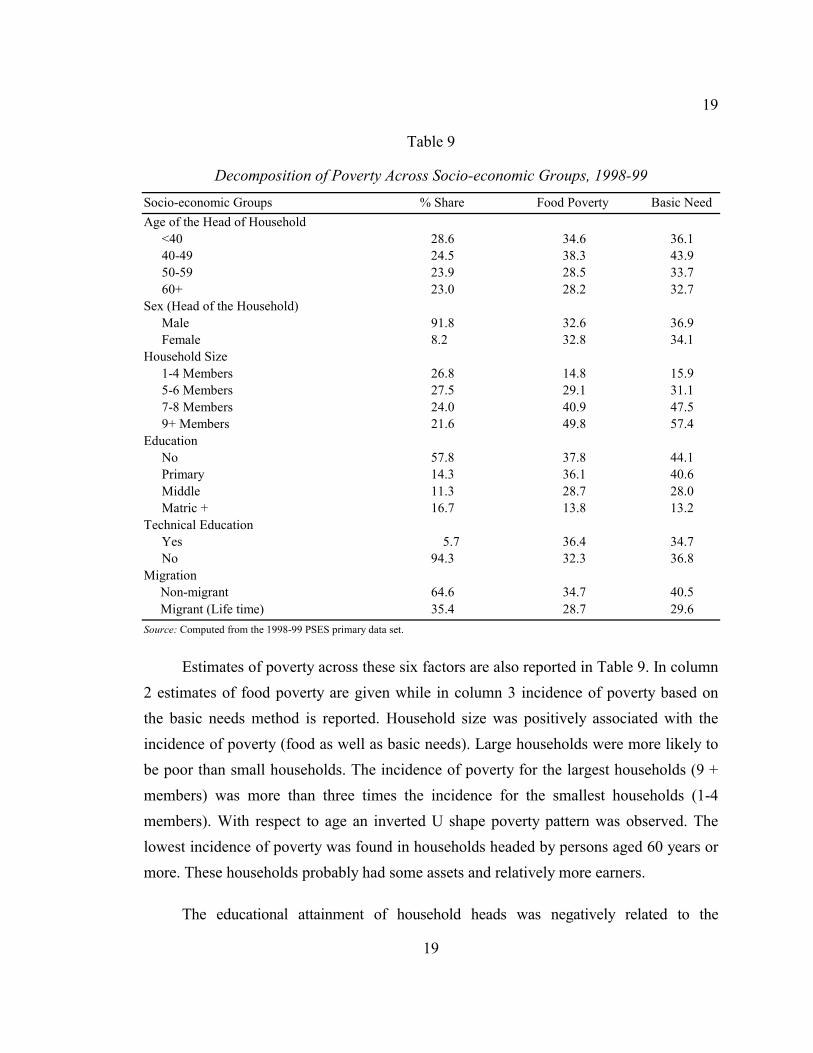
Results of decomposition of poverty by other socio-economic groups are
presented in Table 9, which shows that about 46 percent of households in Pakistan
had in 1998-99 seven members or more. Average household size was 6.4 (not
reported in Table 9). About half of household heads were 50 years old or more.
Females headed only 8 percent of households. More than half of the household heads
were illiterate. And about 17 percent had completed at least 10 years of schooling.
Only 6 percent of the head of households had some technical education. Table 9
further reveals that more than one-third of them migrated from elsewhere to their
current place of residence.
19
19
Table 9
Decomposition of Poverty Across Socio-economic Groups, 1998-99 Socio-economic Groups % Share Food Poverty Basic Need Age of the Head of Household <40 28.6 34.6 36.1 40-49 24.5 38.3 43.9 50-59 23.9 28.5 33.7 60+ 23.0 28.2 32.7 Sex (Head of the Household) Male 91.8 32.6 36.9 Female 8.2 32.8 34.1 Household Size 1-4 Members 26.8 14.8 15.9 5-6 Members 27.5 29.1 31.1 7-8 Members 24.0 40.9 47.5 9+ Members 21.6 49.8 57.4 Education No 57.8 37.8 44.1 Primary 14.3 36.1 40.6 Middle 11.3 28.7 28.0 Matric + 16.7 13.8 13.2 Technical Education Yes 5.7 36.4 34.7 No 94.3 32.3 36.8 Migration Non-migrant 64.6 34.7 40.5 Migrant (Life time) 35.4 28.7 29.6 Source: Computed from the 1998-99 PSES primary data set.
Estimates of poverty across these six factors are also reported in Table 9. In column 2 estimates of food poverty are given while in column 3 incidence of poverty based on the basic needs method is reported. Household size was positively associated with the incidence of poverty (food as well as basic needs). Large households were more likely to be poor than small households. The incidence of poverty for the largest households (9 + members) was more than three times the incidence for the smallest households (1-4 members). With respect to age an inverted U shape poverty pattern was observed. The lowest incidence of poverty was found in households headed by persons aged 60 years or more. These households probably had some assets and relatively more earners.
The educational attainment of household heads was negatively related to the
20
20
incidence of poverty. Those households whose heads had no education had the highest
poverty. It was about three times the incidence of poverty among households whose heads
had completed at least 10 years of schooling. The pattern was the same for food poverty as
well as for poverty estimates obtained using the basic needs approach. Technical education,
however, did not show any consistent pattern. Incidence of poverty was lower among those
heads of households who moved in the past to their current place of residence. Migration
has probably provided them with an opportunity to move out of the poverty.
7. DETERMINANTS OF POVERTY
To examine the determinants of poverty, multivariate analyses were also carried out.
The 1998-99 PSES data set was used in these analyses. Two models were estimated: model 1
focused on food poverty; and determinants of poverty based on the basic needs approach
were examined in model 2. The dependant variable in these models takes the value of one if
poor and zero otherwise. Ten explanatory variables were entered into these models. Age of
the head of households in completed years was included in the model. Sex of the head of
household takes a value of one if the head was male and zero if female. Four levels of
educational attainment were represented by three dummy variables. The first variable takes
the value one if the head of household was educated to primary level and zero otherwise. The
second variable represents the middle level, and was coded one if the head was in this
category and 0 otherwise. The third variable takes the value one if the head of household was
educated to matriculation or higher level and zero otherwise.
Similarly four categories of household size were represented by three dummy
variables. Technical education is a dichotomous variable that takes the value one if the
head of household had some technical education and zero otherwise. Farm status of
household was also a dichotomous variable. The type of place of residence, rural and
urban, was entered in the models as dummy variable. The rural area was the reference
category. Three categories of the duration of residence were represented by two dummy
variables. The first variable takes the value one if head of household has been living at
current place of residence for less than 10 years and zero otherwise. The second variable
21
21
takes the value one if the duration of continuous residence was 10 years or more and zero
otherwise. The number of earners in a household was entered in the two models as a
continuous variable. The last variable, remittances, is a dichotomous variable that takes
the value one if a household received remittances from abroad or within the country
during the year preceding the survey and zero otherwise.
As the dependant variable in two models was binary, logistic regression was used.
The results (odds ratios) are presented in Table 10. A logit estimate was considered to be
significant if it was at least double the associated standard error value. At the bottom of
each column of the table (model) are the relevant number of cases and the value of –2 log
likelihood.
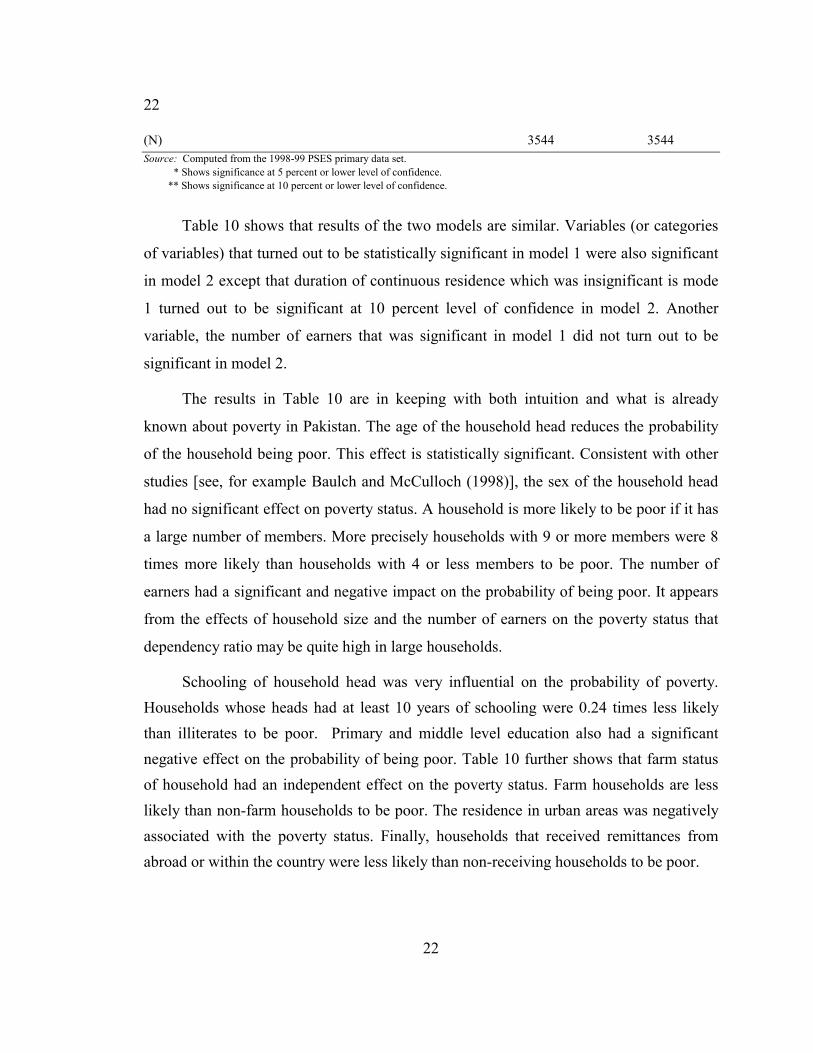
Table 10
Logistic Regression Effects of Predictors on Being Poor (Odds Ratios) Model 1 Model 2 Predictors Food Poverty Basic Needs Age of the Head of Households (Years) 0.98* 0.98* Sex of the Head of Household (Male = 1) 0.97 0.99 Household Size
Education of the Head of Household Illiterate 1.00 1.00 Primary (1-5 Years Schooling) 0.74* 0.77* Middle (6-9 Years Schooling) 0.54* 0.45* Matriculation and Above (10+ Years Schooling) 0.24* 0.22*
Technical Education (Yes = 1) 1.12 0.84 Farm Status of Households (Farm = 1) 0.55* 0.61* Duration of Continuous Residence (Head Only)
Since Birth 1.00 1.00 < 10 Years 1.08 0.99 ≥ 10 Years 0.96 0.85**
Place of Residence (Urban = 1) 0.56* 0.31* Number of Earners in a Household 0.89* 0.96 Remittances (Receiving = 1) 0.69* 0.63* –2 Log Likelihood 3963 3852
22
22
(N) 3544 3544 Source: Computed from the 1998-99 PSES primary data set. * Shows significance at 5 percent or lower level of confidence. ** Shows significance at 10 percent or lower level of confidence.
Table 10 shows that results of the two models are similar. Variables (or categories
of variables) that turned out to be statistically significant in model 1 were also significant
in model 2 except that duration of continuous residence which was insignificant is mode
1 turned out to be significant at 10 percent level of confidence in model 2. Another
variable, the number of earners that was significant in model 1 did not turn out to be
significant in model 2.
The results in Table 10 are in keeping with both intuition and what is already
known about poverty in Pakistan. The age of the household head reduces the probability
of the household being poor. This effect is statistically significant. Consistent with other
studies [see, for example Baulch and McCulloch (1998)], the sex of the household head
had no significant effect on poverty status. A household is more likely to be poor if it has
a large number of members. More precisely households with 9 or more members were 8
times more likely than households with 4 or less members to be poor. The number of
earners had a significant and negative impact on the probability of being poor. It appears
from the effects of household size and the number of earners on the poverty status that
dependency ratio may be quite high in large households.
Schooling of household head was very influential on the probability of poverty. Households whose heads had at least 10 years of schooling were 0.24 times less likely than illiterates to be poor. Primary and middle level education also had a significant negative effect on the probability of being poor. Table 10 further shows that farm status of household had an independent effect on the poverty status. Farm households are less likely than non-farm households to be poor. The residence in urban areas was negatively associated with the poverty status. Finally, households that received remittances from abroad or within the country were less likely than non-receiving households to be poor.
23
23
8. CONCLUSION
This study was designed to estimate the incidence of poverty for the more recent
period, 1998-99. Poverty differentials across rural/urban areas, farm status of the
households and other socio-economic groups were also examined. Determinants of
poverty were explored by using logistic regressions. This study used two primary data
sets: the 1993-94 HIES and 1998-99 PSES. Two methods, FEI and CBN, were applied to
estimate the incidence of poverty.
At the national level about one-third households were below the food poverty line
in 1998-99. Under the basic needs approach the incidence of poverty was at least 35
percent for this period. The results of this study support the view that the recent rise in
poverty, which started in the early 1990s, continued at the end of decade. More rural
households were poor than urban households. Still, in 1998-99, a quarter of urban
households were below the poverty line. Within rural areas, the incidence of poverty was
higher among non-form households as compared to farm households.
The results of logistic regressions are in keeping with the generally accepted
theory. Having a large household is generally correlated with poverty status, as greater
number of earners in a household increases earning potential and therefore decreases the
risk of poverty. Similarly educational attainment is a critical determinant of the incidence
of poverty and should be considered closely in implementing poverty alleviation
programmes. An increase in the schooling of one individual not only has an impact on
that individual’s productivity and hence earnings, but may also influence the productivity
and earning of others with whom that individual interacts. Landlessness in rural areas is
likely to be associated with poverty. Provision of employment opportunities in rural areas
may reduce the risk of poverty. In short, the present study has determined that policy-
influenced variables such as schooling and employment creation are important factors
that can lead to a significant reduction in poverty levels.
24
24
Appendices
Appendix Table 1
Distribution of the Sample PSUs and SSUs with their Urban/Rural and Provincial Break-down, 1998-99 PSES and 1987-88 HIES
Province/ Number of Sample PSUs Number of Sample SSUs Survey Total Rural Urban Total Rural Urban The 1998-99 PSES
Calorie Requirement by Age and Sex Age Both Sexes Male Female
0-1 Year 1010 – –
2-3 Years 1325 – –
4-5 Years 1550 – –
6-7 Years 1710 – –
8-9 Years 1875 – –
10-12 Years – 2180 2200
13-15 Years – 2500 2300
16-19 Years – 2950 2100
20-39 Years – 2550 2160
40-49 Years – 2420 2050
50-59 – 2300 1940
60+ – 2040 1730
25
25
26
26
REFERENCES
Ahmed, M. (1993) Choice of a Norm of Poverty Threshold and Extent of Poverty in Pakistan. The Journal of Development Studies 12: Peshawar.
Ali, Salman Syed, and Sayyid Tahir (1999) Dynamics of Growth, Poverty and Inequality in Pakistan. The Pakistan Development Review 38:4.
Amjad, Rashid, and A. R. Kemal (1997) Macro-economic Policies and their impact on Poverty Alleviation in Pakistan. The Pakistan Development Review 36:1.
Arif, G. M., and Sabiha Ibrahim (1998) Diarrhoea Morbidity Differentials among Children in Pakistan. The Pakistan Development Review 37:3.
Arif, G. M., S. Mubashir Ali, Zafar Mueen Nasir, and Nabeela Arshad (1999) An Introduction to Pakistan Socio-economic Survey, PIDE, MIMEO.
Baulch, Bob, and Neil McCulloch (1998) Being Poor and Becoming Poor: Poverty Status and Poverty Transitions in Rural Pakistan. Brighton: Institute of Development Studies.
Deaton, Angus (1998) The Analysis of Household Survey: A Microeconomic Approach to Development Policy. Washington, D. C.: The World Bank.
Ercelawn, A. (1990) Absolute Poverty in Pakistan: Poverty Lines, Incidence, Intensity. Applied Economic Research Centre, University of Karachi. (Draft Paper.)
Gazdar, H., S. Howes, and Salman Zaidi (1994) Poverty in Pakistan, Measurement Trends and Patterns, ST/CRD, LSE, London.
Heganaars, A., and Klass de Vos (1988) The Definition and Measurement of Poverty; The Journal of Human Resources 23:2.
Jafri, S. M. Younis (1999) Assessing Poverty in Pakistan. In A Profile of Poverty in Pakistan. Islamabad: Mahbub ul Haq Centre for Human Development.
Jafri, S. M. Yunous, and A. Khattak (1995) Income Inequality and Poverty in Pakistan. Pakistan Economic and Social Review 33.
Malik, M. H. (1988) Some new Evidence on the Incidence of Poverty in Pakistan. The Pakistan Development Review 27:4.
Malik, Sohail J. (1992) Rural Poverty in Pakistan: Some Recent Evidence. The Pakistan Development Review 31:4.
27
27
Nasir, Zafar Mueen (1999) Poverty and Labour Market Linkages in Pakistan. Paper presented at the MIMAP Workshop held in Islamabad on November 9, Pakistan Institute of Development Economics, Islamabad.
Pakistan, Government of (1996) Household Income Expenditure Survey, 1993-94. Islamabad: Statistics Division.
Panagides, Alexis (1994) Mexico. In G. Psacharopoulos and H. A. Patrinos (eds) Indigenous People and Poverty in Latin America: An Empirical Analysis. World Bank Regional and Sectoral Studies, Washington, D. C.: The World Bank.
Pickney, Thomas C. (1989) The Demand for Public Storage of Wheat in Pakistan. Washington: International food Policy Research Institute. (Research Report 77.)
Quinones, Benjamin Jr. (1999) Eradicating Poverty in the Asia-Pacific Region, Asia-Pacific Development Monitor. Journal of the Asian and Pacific Development Centre 1:1.