91
Profitability as a criterion in key account selection -Evidence from a professional services organization Johannes Wellmann Department of Marketing Hanken School of Economics Helsinki 2016

Profitability as a criterion in key account selection-Evidence from a professional services organization
Johannes Wellmann
Department of Marketing
Hanken School of Economics
Helsinki
2016

HANKEN SCHOOL OF ECONOMICS
Department of: Marketing Type of work: Master’sThesis
Author: Johannes Wellmann Date: 22.04.2016
Title of thesis: Profitability as a criterion in key account selection
-Evidence from a professional services organization
Abstract:
Business-to-business companies within the professional services sector tend to
encounter fierce competition when aiming to win over the most distinguished
customers. To avoid unprofitability, these companies need to put much consideration
into prioritizing the right type of customers. However, there is not much academic
literature published on customer prioritization, i.e. key account (KA) selection.
The aim of the study is to measure the relationship between KA selection and customer
account profitability when taking to account other KA selection criteria in a
professional services organization. The study uses internal and external customer data
that is obtained from a professional services organization.
Several quantitative tests such as ANOVA and binary logistic regression were utilized
in the study. Furthermore, AIC, BIC and likelihood ratio tests are used in order to
make valid comparisons between models.
The results show that there is a relationship between profitability and KA selection
when profitability is measured in monetary terms. However, no relationship could be
found when profitability is measured as a percentage. Further tests even indicate that
profitability has not been used as a KA selection criterion, but instead is a by-product
of the fact that KAs have bigger contracts and therefore provide higher account
revenues. Furthermore, customer size, higher account revenue and a higher number of
sales opportunities increase the odds of being selected as a KA, whereas a long
business relationship does not.
Keywords: B2B, Key Account Management, Strategic Account Management, Key
Account Selection, Profitability, Customer Profitability, Professional Services.

CONTENTS
1 INTRODUCTION.................................................................................... 11.1 Research problem ....................................................................................................2
1.1 Aim of the study....................................................................................................... 3
1.2 Limitations of the study .......................................................................................... 3
1.3 Research approach ..................................................................................................4
2 THEORETICAL FRAMEWORK ............................................................ 52.1 Introduction to KAM ............................................................................................... 5
2.1.1 Evolution of KAM ....................................................................................... 5
2.1.2 The role of KAM .......................................................................................... 7
2.1.3 Success factors in KAM ............................................................................. 8
2.2 KAM in professional services organizations ........................................................ 10
2.2.1 The definition of professional services.................................................... 10
2.2.2 Characteristics of KAM in professional services organizations............. 12
2.3 Selection of key accounts ...................................................................................... 14
2.3.1 Relevance of key account selection ......................................................... 15
2.3.2 Selection criteria ....................................................................................... 17
2.4 The role of profitability in KAM .......................................................................... 20
2.4.1 The effect of KAM on profitability .......................................................... 20
2.4.2 Profitability as a measurement ............................................................... 22
2.5 Summary of the theory and literature................................................................. 24
2.5.1 Effects on KA selection ............................................................................ 26
3 DATA ................................................................................................... 283.1 Data description ................................................................................................... 28
3.1.1 The data timeframe ................................................................................. 30
3.2 Variables used in the study ................................................................................... 31
3.2.1 KA priority status: KA vs. OA (KPS) ...................................................... 33
3.2.2 Account revenue (AR) ............................................................................. 33
3.2.3 Gross profit (GP) ..................................................................................... 34
3.2.4 Gross margin as a percentage (GMP)..................................................... 34
3.2.5 Total assets of the customer (TA) ........................................................... 34
3.2.6 Customer relationship length (RL) ......................................................... 35
3.2.7 Sales opportunities identified (SOI) ........................................................ 35

3.2.8 Publically traded (PT) ............................................................................. 36
3.2.9 Customer industry (CI) ........................................................................... 36
3.2.10 Customer headquarter country (HQ) ...................................................... 37
3.3 Sample and other possible data biases ............................................................... 38
3.4 Descriptive statistics ............................................................................................ 38
3.4.1 Continues variables ................................................................................. 38
3.4.2 Categorical variables ............................................................................... 40
4 ANALYSIS METHODS ........................................................................ 434.1 Research question one ......................................................................................... 43
4.2 Research question two ......................................................................................... 44
4.3 Model assumptions .............................................................................................. 48
4.3.1 One way ANOVA ...................................................................................... 48
4.3.2 Binary logistic regression ........................................................................ 49
5 EMPIRICAL RESULTS ........................................................................ 505.1 Results related to research question one ............................................................ 50
5.2 Results related to research question two .............................................................52
6 DISCUSSION ....................................................................................... 586.1 Profitability as a KA selection criterion .............................................................. 58
6.2 Other KA selection criteria ...................................................................................59
6.3 Reliability and validity of the study...................................................................... 61
7 CONCLUSIONS ................................................................................... 637.1 Concluding remarks ............................................................................................. 63
7.2 Theoretical contribution and managerial implications ..................................... 64
7.3 Suggestions for further research ..........................................................................65
SVENSK SAMMANFATTNING ............................................................... 67
REFERENCES ..........................................................................................75

APPENDICES
Appendix 1 ........................................................................................................................... 80
Appendix 2 ........................................................................................................................... 84
TABLES
Table 1 Findings of Guesalga and Johnston (2010) literature review ...........................2
Table 2 Information of the customer sample ............................................................... 30
Table 3 Descriptive statistics of continuous variables ................................................. 39
Table 4 Descriptive statistics of the KA priority status (KPS) variable ....................... 40
Table 5 Descriptive statistics of the publically traded (PT) variable ........................... 40
Table 6 Descriptive statistics of the customer industries (CI) control variable .......... 41
Table 7 Descriptive statistics of the Customer HQ country (HQ) control variable.... 42
Table 8 Results of ANOVA 1 ........................................................................................... 50
Table 9 Results of ANOVA 2 ........................................................................................... 51
Table 10 Results of ANOVA 3 ...........................................................................................52
Table 11 Correlation matrix between the predictive independent variables................. 53
Table 12 Results from the main model binary logistic regressions ...............................54
Table 13 Results from the alternative model binary logistic regressions ......................56

FIGURES
Figure 1 Characteristics of KAM (Ojasalo 2001a).............................................................6
Figure 2 An illustration of the connection between KA selection and KAM .................25
Figure 3 The KA selection process ................................................................................... 27
Figure 4 Illustration of the data timeframe ..................................................................... 31
Figure 5 Illustration of the data timeframe with all variables included ...................... 32

1
1 INTRODUCTION
The business-to-business landscape has been changing rapidly during the last two
decades. One of the most critical changes has to do with the complexity of business-to-
business relationships. These relationships have become more complex due to the
increased expectations of the customer and the cost pressures of the seller (Jones et al.
2005). The required technical know-how, communication skills, industry knowledge
and response-time of sellers have increased the need for active account management
(Jones et al. 2005).
There are many types of interpretations of the nature of account management, which
have resulted in a variety of definitions, account management (AM) roles and AM
programs (Ojasalo 2001a). For instance, key account management (KAM), which
refers to managing the most important customers, is commonly used in organizations
where confidentiality and trust are essential for a functioning business relationship
(Skaates & Seppänen 2002; Nätti & Palo 2008). Also, KAM is utilized by companies
that have to do business with large customers that usually expect special treatment and
a considerable time investment (Pels 1992; Ojasalo 2001a). However, a large customer
does not necessary indicate that it is more profitable for the seller, due to the fact that
larger customers require more of a seller’s time and resources (Sharma 1997; Piercy &
Lane 2006). Therefore, the challenge is to find ways to prioritize accounts not only
based on sales volumes but also profitability and future outlook.
Many companies, especially professional services organizations, are operating in an
extremely competitive environment (Nätti & Palo 2012). In this type of business
environment there is a tendency of being easily forced to a price war when aiming to
win over the biggest and most distinguished customers (Piercy & Lane 2006). As a
result, the seller may win the customers’ business but suffer from the unprofitable
business relationship in the long term. This may lead to worsening business
relationships and bad service quality, which affects the seller’s reputation (Piercy &
Lane 2006). Therefore, an unprofitable business relationship cannot continue in the
long term.
Consequently, it is essential for the sellers to not only prioritize large customers that
expect to be prioritized, but to also to prioritize customers that are actually contributing
the seller’s profitability and thereby increasing the seller’s financial performance.
(Sharma 1997).

2
1.1 Research problem
The role of key account management is a widely discussed topic by practitioners and
academia. Since the topic is widely discussed, there are a lot of definitions and
interpretations of what constitutes KAM. Early academic literature characterizes KAM
as special treatment in areas of service, marketing and administration to specific
customer groups (Barett 1986; McDonald 1997). On the other hand, a more recent and
widely referred definition is presented by Ojasalo (2001a) that defines KAM as
identification and analysis of key accounts in order to create strategic and operational
capabilities to enhance customer relationships. To avoid confusion in the interpretation
of terminology, Homburg et al (2002) have simply described KAM as all activities that
have to do with managing the most important customers.
Table 1 Findings of Guesalga and Johnston (2010) literature review
Topic In Numbers In percentages (%)SAMA Academic SAMA Academic
Organizing for KAM 20 12 19 12Adaptation of KAM approaches 17 11 16 11Success factors in KAM 12 11 11 11Global account management 11 9 10 9Role and Characteristics of KA managers 11 9 10 14Customer relationships 11 14 10 14Team selling 10 5 9 5Selection of key accounts 9 9 8 9Reasons to adopt KAM 3 13 3 13Elements of a KAM program 3 9 3 9
Total 107 102 100 100
In order to have a better understanding of the available KAM literature, Guesalga and
Johnston (2010) made a literature review that takes into account research from both
academics and practitioners. The results from the literature review in question are
summarized in table 1. The sample that represented the practitioners was taken from
the Velocity magazine, published by the Strategic Account Management Association.
The members of the association are executives and consultants working with KAM. The
results of the study are presented in figure 1. They indicate that the most researched
KAM topics amongst academics and practitioners are: how to organize KAM, how to
adapt KAM processes and success factors in KAM. Other interesting insights from
Guesalga and Johnston (2010) literature review are for instance that KAM research

3
have clearly evolved during the past two decades. Also, most of the KAM research has
utilized qualitative methods, but there has been a notable increase in the use of more
complex quantitative methods in later years (Guesalga & Johnston 2010).
However, one of least researched topics in KAM according to Guesalga and Johnston
(2010) is the selection of key accounts. The studies that Guesalga and Johnston (2010)
refer to when discussing the selection of key accounts are Pels (1992) and Sharma
(1997). Both of the studies can be considered relatively old, especially if the statement
that the KAM literature has evolved is correct. Furthermore, most on the studies of
KAM is focused on production companies despite that Nätti and Palo (2012) have
clearly recognized that KAM is widely used in professional services organizations.
Consequently, there is a clear need to address the question of how to select and
prioritize customers from a KAM point of view. The lack of KA selection literature is
evident per se, but lack is even more apparent in the service literature.
1.1 Aim of the study
The aim of the study is to measure the relationship between KA selection and customer
account profitability when taking to account other KA selection criteria in a
professional services organization.
The following research questions are addressed:
Rq1: Does customers’ account profitability significantly differ between a key
account and other accounts in a typical professional services organization?
Rq2: Is customer account profitability a significant predictor of a customer to be
selected as a KA when other probable KA selection criteria are taken to account?
1.2 Limitations of the study
This study uses the assumption made by Homburg et al (2002), which suggests that
KAM involves all activities that have to do with managing the most important
customers. As a result, the study focuses only on different KA selection criteria/metrics
and not on other KAM related activities. The customer profitability measures used in
the study describes only current profitability and is utilized as KA selection criteria.
Therefore, no estimates of the future customer profitability are made. Also, the study

4
utilizes data from a company that have several key account selections based on its
customers’ geographical location. Consequently, this study has its focus on the Nordic
key account selection, which consists of companies that have its headquarters in the
Nordic region.
1.3 Research approach
The study in question consists of both a theoretical discussion and an empirical study.
The theoretical framework is built upon four themes that are relevant to the empirical
study. The latest and the most relevant literature are presented and discussed within
each of the themes in order to get a holistic view of the various aspects of the study.
The empirical study is based on data acquired from a global professional services
organization. The company is referred in this study as company X. The focus of this
study is on analyzing the KA selection of company X quantitatively, by utilizing internal
and external customer data. The variables used in the analysis consists of both
customer profitability related data and other data that have been recognized as relevant
criteria for KA selections by earlier academic literature. This data is analyzed with the
help of several quantitative analysis methods. Lastly, the result from the empirical
study is discussed and compared with the earlier literature.

5
2 THEORETICAL FRAMEWORK
As mentioned in the research approach, this chapter consists of four main themes. The
first theme introduces KAM from several points of views in order to get a better
understanding of the phenomenon itself. The second theme of this chapter revolves
around professional services organizations, and how these types of organizations utilize
KAM, since the empirical study has its focus on a professional services organization.
The third theme addresses the most important topic of the empirical study, which is the
actual KA selection process. As KA selection is a crucial part of KAM, it is important to
get a holistic view of KAM before discussing the KA selection literature. Lastly, the role
of profitability in KAM and KA selection is discussed due to the fact that the empirical
study focuses on the customer profitability.
2.1 Introduction to KAM
From the introduction it could be concluded that there is variety of definitions of KAM.
The underlying reason for this has to do with the fact that KAM is not a straightforward
process and it is often tailored in accordance with customer expectations and wishes.
However, there are a large variety of theories of what constitutes KAM. Therefore, this
chapter intends to give a brief explanation to the evolution of KAM, what kinds of
activities do KAM include and what can be considered successful KAM.
2.1.1 Evolution of KAM
During the late 1950’s and the 1960’s there could be observed a clear shift in business-
to-business selling strategies due to changes in the business landscape (Weilbaker &
Williams 1997). There started to emerge a trend where a few bigger companies usually
accounted for most of a seller’s revenues (Weilbaker & Williams 1997). Up to this point,
sales responsibilities were usually dived by geographical grounds, which led to
variations in price, quality and service. Bigger buyers, with business operations in
several locations and countries started to question this type of business model and
demanding clearer communication and more uniform delivery. (Coletti & Tubidy 1987;
Weilbaker & Williams 1997).
Consequently, many sellers responded by naming a single person to be responsible of a
specific customer (Shapiro & Wyman 1981). This person was given the responsibility
to take care of the communication with the customer and to manage the internal

6
coordination of activities and costs, which were related to the customer in question
(Shapiro & Wyman 1981). This type of behavior started to be recognized by academics,
and themes such as relationship management, international account coordination and
national account management started to emerge in the journals (Shapiro & Wyman
1981). In more recent literature, most of the scholars have used the term “key account
management” when referring to the actual phenomenon and term “account” when
referring to a customer (Ojasalo 2001a).
KAM literature evolved a lot during the last decades according to Guesalga and
Johnston (2010) and took influence from many research fields such as relationship
marketing, sales management and supply chain management (McDonald et al. 1997).
To get a better understanding of the essence of KAM, Ojasalo (2001a) identified various
characteristics of KAM, which are illustrated in Figure 1.
Figure 1 Characteristics of KAM (Ojasalo 2001a)
Emphasis Equallyemphasized Emphasis
Transactional marketing/short-term approach
Relationship marketing/long-term approach
Strategic Operational
Theoretical/descriptive Managerial/normative
Consumer market Business-to-business market
Goods ServicesGoals: Profitability andshareholder value
Goals: Sales volume, marketshare, margin, etc.
According to Ojasalo (2001a) KAM is strongly relationship orientated and focuses on
long-term value creation. The strong relationship orientation is the clearest difference
between a standard account and a key account. KAM consist of both strategic
marketing and operational involvement to ensure that a relationship with a key account
is developed in the right direction. Furthermore, the academic KAM literature is not
only theoretical but also aims to create value for practitioners. Most of the literature is
focused on the business-to-business landscape and are applicable for both services and
goods industries. Lastly, the ultimate goal of KAM is long term profitability and
increasing shareholder value. (Ojasal0 2001a)

7
There has also evolved an alternative, or more of a complementary, way of
understanding KAM, which is based on the notion of service-dominant logic introduced
by Vargo & Lusch (2004). S-D logic is based on the several foundational premises, but
the main point is that companies in business relationships should aim to co-create
value together and not separately take advantage of one another (Vargo & Lusch 2004).
Storbacka (2012) has discussed the role of KAM from an S-D logic perspective and
suggest that key account selling or management is not the same thing as strategic
account management. According to Storbacka (2012) SAM “focuses on co-creation of
value and is both ‘inside – out’, that is implements strategy in order to achieve agreed
corporate goals, and ‘outside-in’, that is identifies business and renewal opportunities
by deeply understanding the customer’s value-crating process, and influences the
firm’s strategic process.” In other words, SAM can be considered as creating and
maintaining relationships with the most important stakeholders in a way which
resembles partnerships, whereas KAM focuses more how to create and maintain long
lasting and profitable relationships with the most important customers. However, some
academics do not see a substantial difference between these two views and therefore do
not categorize them separately (Davies & Ryals 2014).
2.1.2 The role of KAM
As argued in the last section, KAM can be seen from several perspectives. The same
applies when discussing about what KAM is in practice. Because of this, Homburg et al.
(2002) conceptualized four dimensions of KAM; activities, actors, resources and
formalization.
According to Homburg et al. (2002) model, the activities perspective answers the
question: what is done? There are activities such as customized pricing, customized
services and products, tailored customer service, information sharing, joint
coordination of workflow and taking over functions outsourced by the customer
(Homburg et al. 2002). All of these KAM activities are supposed to increase customer
loyalty, customer satisfaction and share of wallet (Homburg et al. 2010). Share of wallet
refers to the expense percentage of a customer’s total expenses that a company could
potentially spend on the seller’s products or services (Homburg et al. 2010).
The actor perspective answers the question: who does it? There are KAM involvement
both on horizontal level, which quantifies time spent on KAM, and vertical level, which
focuses on hierarchical aspects (Homburg et al. 2002). From a horizontal point of view,

8
there are staff members that work with KAM full-time and staff that have a KAM role in
addition to their main duties (Homburg et al. 2002). From a vertical point of view,
there are both top level management and entry level work force involved in KAM
(Homburg et al. 2002). The combination of vertical and horizontal level contribution
depends largely on the business and industry in question. However, it is noted that top
level management involvement is important due to the strategic nature of KAM
((McDonald 1997; Guesalga 2014). Also, KAM is in most cases a coordinated effort
between formal or semi-formal teams (McDonald 1997).
The resources perspective answers to the question: with whom is it done? This question
is closely linked to the previous one. Hence, one of the most important success factors
of KAM is that the right people get access to relevant information (McDonald 1997;
Homburg et al. 2002; Salojärvi et al. 2010). The access to information requires
collaboration, not only between sales and marketing, but also between IT, logistics,
manufacturing, finance and accounting (Homburg et al. 2002). Collaboration is also
required between industry branches/service lines, multiple countries and cultures
(McDonald 1997). Therefore, it is crucial that the staff responsible of KAM have the
necessary authority to coordinate internally within the organization (McDonald 1997;
Salojärvi et al. 2010).
Lastly, the formalization perspective answers the question: how formalized is it?
Companies KAM programs tend to differ from each other in both complexity and intra-
organizational acceptance (Homburg et al. 2002). Therefore, the level of formality of a
KAM program is an important factor to consider when analyzing a company’s KAM
processes (Homburg et al. 2002). In some companies there are global standards on
how KAM is applied, reported and evaluated (Homburg et al. 2002). On the other
hand, KAM may also be a very informal and approached with a case-by-case mentality
(Wengler et al. 2006). Many companies even admit that they do not utilize KAM, but
still informally give special treatment to the most important customers (Wengler et al.
2006). Wengler et al. (2006) calls this type of behavior as “hidden key account
management”.
2.1.3 Success factors in KAM
There are several studies that discuss what makes KAM successful (Guesalga and
Johnston 2010). The success factors vary a lot depending on culture and industry
specific contexts. However, there are some success factors that have been cited and

9
confirmed frequent times by several academics and practitioners, which can be applied
to nearly every KAM case.
One of the most important success-factors is directly related to the knowledge and
capabilities of the key account manager (McDonald 1997; Abratt & Kelly 2002;
Guesalga 2014). A KA manager should be highly skilled in areas such as negotiation,
managing relationships, marketing and finance (Abratt & Kelly 2002). To exemplify the
role of the KA manager, McDonald (1997) draws a parallel - “The key account manager
conducts the orchestra”. Also, the KA manager should have a formal or semiformal
team. The team should be cross-functional, because it has been recognized that cross-
functionality increases the awareness of the value of KAM practices internally,
especially of efforts that is hard to measure in monetary terms (Abratt & Kelly 2002).
Another important success-factor is to truly understand a key account’s business and
what creates value for it (Abratt & Kelly 2002). To succeed, the KAM team needs to
have tools by which they can gather and store customer information and to be able to
distribute it to the relevant people (Salojärvi et al. 2010). Thus, an integrated CRM
system is necessary for sufficient internal coordination and information distribution
(Salojärvi et al. 2015).
Furthermore, successful KAM usually requires a culture that encourages the pursuit of
customer satisfaction in all company levels (Abratt & Kelly 2002). It is important that
even top management should have customer satisfaction as a top priority, and even be
involved in KAM activities (Guesalga 2014). However, it has been noted that the senior
leadership needs to understand that their involvement should only be limited to
support the underlying KAM strategy (Guesalga 2014). Otherwise there is a risk that
the message to the customer will not be uniformed (Guesalga 2014).
However, it is impossible to succeed in KAM without recognizing which customers
should be selected as KAs. Therefore, a KA selection process is essential for successful
KAM (Abratt & Kelly 2002). Key accounts should be identified in accordance with clear
guidelines (Abratt & Kelly 2002). Also, the selection should be done based on several
financial and nonfinancial criteria that are aligned with the company’s strategic
oversight (Abratt & Kelly 2002; Tzempelikos & Gounaris 2013). The benefits of KAM
will be marginal if the KA selection is done based on the wrong criteria. According to
Piercy and Lane (2006) KAM can become a serious liability if it the companies enrolled
in KAM programs are not in a position where they benefit from a strong relationship

10
with the seller. In these types of situations there is a great risk that the customer will
react negatively to any KAM related activities. Thus, KAM cannot be successful without
appropriate KA selection methods.
Summary: The KAM literature has evolved considerably during the last decades.
Traditionally, KAM has been perceived more as a support function whereas today it is
seen as a strategic choice that influences how a business-to-business company should
operate. Consequently, the KAM literature has become more complex and is strongly
linked with relationship marketing. Companies that utilize KAM needs to have certain
features embedded throughout the organization to benefit from KAM. Thus, companies
need to understand that KAM is a strategic choice and select key customers with
caution. As a result, an efficient KA selection process is considered as a very important
success factor of KAM.
2.2 KAM in professional services organizations
Most of the KAM literature has focused on business-to-business supplier and buyer
relationships, despite the fact that the business-to-business services industries have
been adopting KAM for a long time. KAM is especially relevant to knowledge intensive
service industries, were trust and confidentiality are considered extremely important
(Skaates & Seppänen 2002; Nätti & Palo 2012). The following section discusses what a
professional services organization constitutes in order to get a better understanding of
how KAM should be applied and what kind of KA selection criteria is typical in
professional services organizations.
2.2.1 The definition of professional services
Knowledge intensive services, which are performed by professional services
organizations, usually are referred to as professional services (Nätti & Palo 2012).
However, it is not entirely clear which services can be considered as professional
services (Thakor & Kumar 2000). Thakor and Kumar (2000) aimed to clarify the
notion of professional services, both theoretically and empirically, in order to have a
better understanding of which professions are by definition considered as professional.
According to Thakor and Kumar (2000) there is not a universal understanding of the
definition of professional services - it is a matter of perception. Generally, white-collar
professions, which require expertise and credentials, are seen as more professional
than services that are performed with hands (Thakor & Kumar 2000). Also, services

11
are considered professional when they are seen as homogenous, complex and critical
(Thakor and Kumar 2000).
Services are not traditionally considered homogenous (Dahringer 1991), but when
compared with other types services, a certain type of homogeneity, or replicability, can
be seen as a sign of professionalism (Thakor & Kumar 2000). For instance, a brain
surgeon needs to be able to replicate a specific type of clinical engagement on several
patients. Also, the notion of a professional service being critical in this case refers to
the fact that the service should have an impact on the society (Thakor & Kumar 2000).
However, the clearest differentiator between services in general and professional
services, especially from a business-to-business perspective, has to with the complexity
of the service offerings. The complexity of professional services offerings not only
requires a high level of expertise from the service provider itself, but usually even from
the buyer (Lian & Laing 2007). It is typical that the buying company approaches a
professional services organization with fuzzy, implicit or unrealistic expectations,
because they do not have the expertise needed to make a realistic assessment of the
situation (Ojasalo 2001b). According to Ojasalo (2001b) fuzzy expectations refer to a
situation where a customer does not clearly know what it wants from a service provider,
whereas implicit or unrealistic expectations are expectation misalignments. These
situations arise when the customer recognizes a problem and is confused about how to
solve it (Ojasalo 2001b). Hence, the fuzzy expectations and misalignments of specific
knowledge between the buyer and seller highlight the value of customer references.
Customer references works as proof-of-concept to the buyer and therefore increases the
credibility of the service provider (Skaates & Seppänen 2002). Consequently,
professional services organizations put a lot of effort to build a strong reputation.
Furthermore, the complexity and intangibility of professional services makes continual
interactions between the buyer and service provider a necessity (Lian & Laing 2007).
Usually several interactions occur before, during and after the service provided
(Skaates & Seppänen 2002). Therefore, there is a substantial human element involved
in the service delivery, which require a strong relationship orientation. Ojasalo (2001b)
suggests that professional services organizations should focus on establishing long
lasting relationships. He implies that on the short term, customer satisfaction levels
vary a lot due to expectations misalignments and lack of trust.

12
The strong relationship orientation of professional services can also be perceived by
how professional services organizations develop their competences. According to
(Awuah 2007) market-based learning is as critical for internal competence
development. Professional services firms learn from their customers, competitors and
other actors that are in the reach of their network (Awuah 2007).
2.2.2 Characteristics of KAM in professional services organizations
There is little research on specific characteristics and challenges of KAM in professional
services organizations (Nätti et al. 2006). Therefore, Nätti et al. (2006) conducted a
explorative qualitative case study were two professional services organizations were
studied; one that had been utilizing KAM for a long time, called Factor, and one that
had just started, called Auctor. The results of the case study supports earlier KAM
literature presented in earlier sections, but also highlight specific KAM actions that are
particularly relevant for professional services organizations.
Case Factor had been implementing KAM for years and had a strong culture of highly
prioritizing the pursuit of customer satisfaction. Metrics to measure KAM performance
and incentives had been established to support collaboration within sales and other
internal divisions. The KA managers had been recruited internally and made up of
persons with wide internal networks. Furthermore, KA managers had KAM teams that
consisted of persons from different expertise areas to enhance internal collaboration.
The KA managers were considered the linking pin between the key customers and the
organizational expertise areas. Account specific information gathered from customer
interactions and external sources were stored in detail in an internally shared IT
system. Clear account plans were serially initiated based on the account information
gathered and by involving partly the customer in the planning process. (Nätti et al.
2006)
On the other hand, case Auctor had just adopted KAM. The company had an
individualistic culture and a functional structure with several subgroups. Incentives
and metrics were designed to create competition internally. KA mangers were few and
were recruited outside the organization and thus lacked internal network within the
organization. No official KAM teams were initiated. The KA managers did not have a
linking role internally and was more focused on integrating IT tools in the account
management process. However, customer specific knowledge was not gathered in a

13
common shared system and the communication and cooperation between experts
involved in the same account was weak. (Nätti et al. 2006)
Consequently, case Factor felt that applying KAM deepens the relationships with their
important customers and creates value creation opportunities; whereas case Auctor had
experienced problems already during KAM implementation and did not achieve
noteworthy customer relationship improvements (Nätti et al. 2006). As can be seen for
case Auctor, KAM implementation is not an easy task and can in many cases be a
substantial risk (Piercy & Lane 2006). An organization should not implement KAM if
the structures of the organization do not show elements of “KAM fit” (Piercy & Lane
2006). Furthermore, the success factors of case Factor are clearly in accordance with
the elements of successful KAM, presented in the earlier sections, by i.e. Abratt & Kelly
(2002), Guesalga (2014) and Salojärvi et al. (2015).
However, compared to other types of organizations, professional services organizations
seem to be reliant of effective internal and customer orientated knowledge transfer. As
Nätti et al. (2006) puts it; “The key issue in customer-relationship management (and
in KAM) is to find a match between the customer’s needs and the competence of the
professional organization.” Therefore, it is crucial that KAM practices in professional
services organizations have a strong focus on enhancing information sharing and
collaboration between internal functions, or areas of expertise, to facilitate value
creation opportunities (Nätti & Ojasalo 2008).
Nevertheless, Nätti and Ojasalo (2008) argue that issues related to knowledge transfer
are very common in professional services organizations, due to the fact that they have a
tendency of suffering from loose coupling. According to several literature summarized
by Nätti and Ojasalo (2008), loose coupling refers to mismatches in communication,
collaboration, ideas between people, subgroups or even functions. In other words, a
company suffering from the before mentioned mismatches can be considered loose
coupled. Some level of loose coupling is nearly unavoidable in professional services
organizations due to the nature of the business itself, which purpose is to create
monetary gains from scarce knowledge (Nätti & Ojasalo 2008).
Thus, the most important function of KAM in business-to-business professional
services organizations is to organize and select the KAs in way that enables seamless
coordination internally, in order to achieve the account specific goals (Nätti & Palo
2012). If the goal is to increase account revenue, the KA plan should focus on cross-

14
selling, which requires internal collaboration between cross-functional functions
(Storbacka et al. 2011). The KA selection should in this case be organized in a way that
increases the cross selling opportunities. Or if the goal is to increase account
profitability, the KA team needs to assess the reasons behind the unprofitability and
address them (Sharma 1997).
From a professional service point of view, Nätti and Palo (2012) argues that it is not
enough to have management support, sufficient resources and clear metrics, but also a
balance between coordination and local flexibility. Because professional services are
based on trusted, and even confidential, relationships (Skaates & Seppänen 2002; Nätti
& Palo 2012), it is crucial to have a bit of discretion in KAM implementation (Nätti &
Palo 2012). Relationships between professionals and customers should be addressed in
situations-specific contexts (Nätti & Palo 2012). For instance, parties that can be
critically affected of a specific decision should be involved in the decision-making
process (Nätti & Palo 2012). On the other hand, there is a substantial risk when
involving parties that do not have the same agenda or the “KA management mind-set”,
due to contradicting short term incentives and goals (Piercy & Lane 2006).
Summary: Professional services are seen as homogenous, complex and critical in
nature. This type of business is usually built upon trust and confidence, which makes
the business relationship oriented. Thus, there is a lot of interaction between a
professional services provider and its customers. Internal and external coordination is
very important for professional services organizations, due to the fact that they in many
cases suffer from loose coupling. Loose coupling makes KAM practices challenging to
implement and therefore can be considered a risk if not implemented correctly. Also, a
coordinated and centralized key account selection process may prove challenging in
this type of organization, due to loose coupling, which can cause contradicting short
term incentives and goals.
2.3 Selection of key accounts
As mentioned in the research problem section, selection of key accounts is not a widely
studied topic. The topic cannot be considered “new” or “emerging”, based on the
enormous amount of KAM literature that has been written during the last decades.
However, the importance of key account selection is constantly increasing due to the
rising competition and emergence of new technologies (Gosselin & Bauwen 2006).

15
Therefore, this section is intended to elaborate on why KA selection is a crucial part of
KAM and what kind on criteria should the selection be based on.
2.3.1 Relevance of key account selection
The whole notion of key account selection is bound to the idea that some customers are
better than others. This perception is inherited from the world famous Pareto
Principle, which assumes that 80 percent of specific effects come from 20 percent of
causes (Brynjolfsson et al. 2011). For instance, 80 percent of all sales come from 20
percent of customers (Brynjolfsson et al. 2011). While this notion is not true in all cases
(Brynjolfsson et al. 2011), it is still used quite widely as an assumption when dealing
with uncertainties.
According to Pels (1992) there are two reasons why a seller would choose to work with a
limited amount of customers;
(1) The seller has no choice but to have a restricted amount of customers
(2) The seller has on purpose chosen to do business with only a few customers.
The first reason is directly linked to the sellers own resources and capabilities. A seller
can only attain as many customers it is capable to provide for. Therefore, it is quite
usual that sellers find themselves in a position where they become financially
dependent on a few customers (Pels 1992). These customers understand their power
position and thus require a substantial amount of attention from the seller. Piercy and
Lane (2006) call this phenomenon as the “KAM trap”. They argue that KAM practices
are in many cases destructive because KAM strategies drive businesses towards this
unbalanced power relationship between the buyer and seller (Piercy & Lane 2006).
On the other hand, the situation is different if the seller has deliberately chosen to work
with a restricted amount of customers. In these cases the power balance between the
buyer and seller is neutral, sometimes even opposite. The seller may have obtained a
competitive advantage; such as scares resources, valuable patents or other expertise
(Azzam 1996).
The two cases above illustrates situations were not much efforts have been putted to
create a structural KA selection process, since these companies have either deliberately
or been forced to work with a restricted amount of customers.

16
Still, in most cases sellers tend to take all the business they are able to handle, due to
the pressure from shareholders to grow. Sellers usually have various types of
customers, which all require different amount of attention. In this case a KA selection
process becomes necessary in order to meet the requirements of the more demanding
customers. Consequently, seller needs to understand the customers’ expectations and
how to exceed them (Parasuraman et al. 1991). According to McDonald (1997) a buying
company choses a supplier based on how easy it is to do business with the supplier, the
quality of the product or the service provided and culture match. Furthermore, Sharma
(1997) have recognized that buyers that are multifunctional and have a multi-layered
decision making process tend to prefer KAM practices. The same tendency can also be
seen in large for-profit companies (Sharma 1997).
Despite the buyers’ preferences, the seller needs to make an own evaluation on which
companies is fit for being a key account based on own strategic priorities (Sharma
1997). According to Ojasalo (2002) sellers should ask themselves: ‘‘Which existing or
potential customers are important to us now and in the future?’’ and ‘‘What criteria
determine important customers?’’ These criteria should be based on a selection that
takes to account both non-financial and financial criteria (Pels 1992; Jones et al. 2009).
Nevertheless, there are not any widespread methods available to do this kind of
selection (Wengler et al. 2006); despite the fact that tracking and storing data have
never been easier than today (Salojärvi & Sainio 2015). There are some selection
criteria that are used by sellers, yet in a relatively primitive way (Wengler et al. 2006).
However, according to Homburg et al. (2010), a key account selection does not
necessary work despite of a well-motivated key account selection procedure. Their
study indicates that if a seller lacks the prerequisite of successful KAM, such as senior
level executive involvement, customer information and the right type of incentives, a
key account selection would not correspond with the marketing and resource
allocations in the daily work. In other words, a strategic key account selection will stay
as an intention if the prerequisites for a successful KAM are not met (Homburg et al.
2010). Consequently, a firm has to earnestly evaluate its capabilities before trying to
implement a formal key account selection process.

17
2.3.2 Selection criteria
As earlier mentioned, there are both financial and non-financial KA selection criteria
(Pels 1992; Jones et al. 2009). These selection criteria should not be used singly, but
rather as a mixture, including both nonfinancial and financial once (Pels 1992; Piercy &
Lane 2006; Tzemeplikos & Gounaris 2013). Some of the criteria can also be considered
less important than others, if their impact towards the seller or the customer seems
unnoticeable (Wengler et al. 2006).
Financial KA selection criteria
The most common financial criterion is the current sales volume to an account
(Wengler et al. 2006). Approximately 80 percent of sellers applied the criteria in
question, according to a study by Wengler et al. (2006) focusing on the German
business-to-business market. This measurement is used to prioritize customers based
on how much money the customer is paying to the seller. On the other hand, Pels
(1992) suggest focusing on the future by calculating present and future sales gaps. The
present sales gap refers to the difference between actual sales and potential sales to the
customer, whereas the future sales gap is linked to the estimated growth of the sales
potential (Pels 1992). The present sales gap resembles the term “share of wallet” that
refers to the expense percentage of a customer’s total expenses that a company could
potentially spend on the seller’s products or services (Homburg et al. 2010), which is
more commonly used term by practitioners. However, according to Sharma (1997),
sales volume related criteria are not good for KA selection, because these
measurements does not take to account the costs associated with the customer. In
other words, it does not take to account the actual contribution of a customer, i.e.
customer profitability (Sharma 1997).
A less used by practitioners (Wengler et al. 2006), but even more important (Sharma
1997; Piercy & Lane 2006), financial criterion is customer profitability (McDonald et al.
1997). To measure effectively customer profitability it is important that the seller have
adequate reporting systems, since it requires continues revenue and cost monitoring
per customer (Mulhern 1999). Particularly interesting is that the role of customer
profitability seems to be undermined by practitioners (Wengler et al. 2006), despite the
fact that a high customer profitability rate is one of the most essential metric for a
healthy businesses (Narver & Slater 1990). There are several variations of customer

18
profitability, which are more thoroughly discussed in section 2.4 The role of
profitability in KAM.
Other financial criteria are for example market share, market cap (Wengler et al. 2006)
and the overall turnover of the customer (Czinkota & Wesley 1983). These
measurements are not linked to the seller, but rather explain the size of the customer. A
large market share and big market cap can be considered as indicators of a strong
position in the market, which makes the company “worth knowing”, whereas a higher
overall turnover indicates that a customer have the means to acquire more costs
(Czinkota & Wesley 1983). In other words, these measurements measures how large a
customer actually is (Czinkota & Wesley 1983).
Nonfinancial KA selection criteria
Nonfinancial selection criteria are in reality at least as important to business-to-
business companies as financial once (Tzemeplikos & Gounaris 2013). After all, a
substantial portion of the benefits of KAM are nonfinancial.
Status and image related selection criteria are the most common nonfinancial criteria
(Pels 1992; McDonald 1997; Wengler et al. 2006). These criteria are intangible in
nature (McDonald 1997). According to the study by Wengler et al. (2006) 35 percent of
business-to-business companies admittedly utilize these types of measurements. The
purpose of these criteria is to quantify a customer’s reputation. The selling company is
usually more willing to give special treatment, such as KA status, to customers that can
affect the seller’s reputation positively. For instance, reference value is a very usual
measurement when measuring a customer’s status or image (Tzemeplikos & Gounaris
2013). A seller is prepared to invest more in a customer that can be used as a reference
(Skaates & Seppänen 2002). As earlier mentioned, quality references bring credibility
to a seller, which helps to acquire new customers and attract talent (McDonald 1997;
Skaates & Seppänen 2002). According to Andreassen and Lindestad (1997) corporate
image is a better predictor of customer loyalty than customer satisfaction, when
studying services providers that provides complex services. Therefore, the value of
status and image related selection criteria should not be undermined.
Another nonfinancial criterion is something that Pels (1992) has named as the network
effect. This criterion is linked to the selling companies’ strategic goals. For instance, if
a seller wants to enter a specific new market or get a better position in a certain

19
segment, it can prioritize customers that have the power or the network to positively
influence the targets set (Pels 1992). However, the network criterion should be
combined with other criteria, which are not as intangible in nature (Pels 1992).
Furthermore, selection criteria such as know-how development, relationship length
and geographical location are used by business-to-business companies (Pels 1992;
Wengler et al. 2006; Tzemeplikos & Gounaris 2013). Yet, they are considered less
useful compared to status and image related criteria (Wengler et al. 2006).
Know-how development is used as a criterion when the seller acts within a
technologically advanced market, from which the seller has to continuously learn from
in order to maintain its competitive advantage (Pels 1992). Also, Ojaslo (2002)
recognizes know-how developments as an important selection criterion for knowledge
intensive service companies that do business with buyers with high level of expertise.
Moreover, relationship length is a criterion that is used in businesses that rely on
strong personal relationships between the buyer and seller. Basically, the customers
that have loyally been in business with the seller for a long period of time are enrolled
to the KAM program. This type of selection is very widely used in business-to-consumer
services industry, such as in retail, aviation and hospitality (Meyer-Waarden et al.
2007). Business-to-business companies seem to more seldom use relationship length as
a selection criterion (Wengler et al. 2006).
Lastly, geographical location as a KA selection criterion is not as relevant today as it
was a few decades ago. Customers that acted in several geographical locations usually
had to be enrolled in some kind of KAM program, due to the fact that these customers
required more internal and external coordination from the seller. However, the ICT
technology available today has made companies less dependent on geographical
selection (Gosselin & Bauwen 2006).
Summary: KA selection is based on the notion that some customers are better than
others. Therefore, the purpose of a KA selection is to prioritize customers in according
to specific guidelines that are aligned with the seller’s strategy. These guidelines should
consist of both financial and nonfinancial criteria. A financial criterion might be the
sales volume to the customer, customer profitability, market share, market cap and
turnover. In contrast, a nonfinancial criterion might be customer image, network effect,
know-how development, geographical location and relationship length. The most

20
commonly used criteria are sales volume and customer image, while academics argue
that customer profitability is overlooked.
2.4 The role of profitability in KAM
The role of profitability in KAM is a discussed topic by academics. Many academics
have recognized that profitability should be one of the prime goals of KAM (Jones et al.
2009). However, studies such as Wengler et al. (2006), Piercy and Lane (2006) and
Sharma (1997), denotes that KAM practitioners tend to focus more on nonfinancial
measurements and other financial determinants, such as sales volume, when selecting
key accounts. To enhance the understanding behind this phenomenon, it is crucial to
understand what drives profitability. Therefore, this section is dedicated to elaborate on
what profitability constitutes, how KAM affects profitability and what does this imply
for the KA selection process.
2.4.1 The effect of KAM on profitability
As explained in the “role of KAM” section, all KAM activities are supposed to increase
customer loyalty, customer satisfaction and the customer share of wallet (Homburg et
al. 2010). These measurements are supposed to affect positively the financial
performance of the seller (Homburg et al. 2010). Therefore, it crucial to discuss how
these measurements is actually linked to profitability.
There is a common saying, which indicates that it is five times more costly to win a new
customer as it does to retain an existing one (McDonald et al. 2000). This saying refers
to the fact that there are acquisition costs related with acquiring a new customer, which
do not reoccur after a successful sale (Rust & Zahorik 1993). The retention costs, which
are costs that are associated with retaining a customer, are much less compared the
acquisition costs (Reichheld & Sasser 1990). Therefore, it is important for a seller to not
only win new customers, but to also make sure that the old ones stay. Sellers that have
a good retention rate, i.e. have many customers that continue to use the seller’s product
or service, have a lot of loyal customers (Reichheld & Sasser 1990). The measurement
this for type of activity is called customer loyalty. Companies with loyal customers can
outperform financially companies with less loyal customers, due to the fact that they
have a better retention rate (Reichheld & Sasser 1990). Thus, customer loyalty usually
indicates better profitability. In other words, companies that have a substantial amount
of loyal customers have a less heavy cost burden compared to similar companies with

21
less loyal customers, which affects profitability. However, Reinarz and Kumar (2000)
consider this type of rationale as an oversimplification. They argue that the effect of
customer loyalty to profitability is not as strong in non-contractual relationships. But,
Reinarz and Kumar (2000) agree that customer loyalty has a significant effect on
profitability in contractual relationships, which ultimately all business-to-business
relationships are based on. To elaborate, contractual relationships refer to business
relationships that rely on a business contract, usually in a form of a written document
(Reinarz and Kumar 2000).
Moreover, a study by Anderson et al. (1994) on the Swedish business-to-business
market has found a positive correlation with customer satisfaction and financial
returns. In other words, companies that have more satisfied customers enjoy better
profitability. The study also noted that customer satisfaction has a lagged effect on
financial returns (Anderson et al. 1994), which means that positive financial returns
due to increased customer satisfaction do not appear immediately. Therefore, a long
term approach is essential when analyzing the economic benefits of customer
satisfaction.
Lastly, the share of wallet refers to a percentage or a sum that a customer pays
compared to what the customer could pay if the seller would win all the customers’
business that the seller can handle (Homburg et al. 2010). The effect of share of wallet
to profitability has somewhat the same rationale as customer loyalty. By having already
acquired a customer, an increase in sales to the same customer would only increase the
retention costs a fraction of what acquiring new business would (Rust & Zahorik 1993).
But from a financial point of view, there is a risk that the additional business would
incrementally increase other costs due to additional resource allocation. But, the
resource issue is more a question of effective pricing, which can be done effectively with
relevant customer information (Ryals 2006). By having a customer relationship already
in place means that the seller most likely has a better access to information in relation
to the buyer than companies without an established business relationship. As earlier
mentioned, one the most crucial requirements of successful KAM was access to
customer information (Salojärvi et al. 2010).
Consequently, all of these measurements are not independent of one another. It is well
known that there is a clear correlation between customer satisfaction and loyalty, which
most likely also affects the share of wallet. However, the link between these
measurements and profitability is ultimately quite vague. Therefore, a company should

22
not only focus on increasing the customer satisfaction, customer loyalty and the share
of wallet separately but also take the profitability of the customer to account when
selecting KAs.
2.4.2 Profitability as a measurement
A business cannot continue without being profitable in the long term (Narver & Slater
1990). That is why profitability is the essence of business. However, there are
alternative ways of understanding and measuring profitability. It is important to
understand the difference of profit and profitability (Goodman 1970). Profit is a static
historical term that is used for reporting purposes, whereas profitability is a dynamic
term that is calculated to support decision making (Goodman 1970). Alternatively,
some argue that profitability is just a historical measure that explains which customers
are not making a loss for a company. In other words, profitability can be viewed as
measurement that is calculated form historical profit data but used for predicting the
future, or alternatively, just as another historical measurement.
Still, profitability measurements are used by decision makers, especially marketers, to
motivate and quantify specific types of actions or activities (Goodman 1970). For
instance, a foundation in relationship marketing theory is that it is more beneficial to
establish long-term customer relationships than short-term (Reinarz and Kumar
2000). The term “beneficial” in this case ultimately refer to increased profitability.
Profitability can be measured in many ways depending on the context. Therefore, it is
crucial to understand the context form which a specific profitability measure is used
for. Generally, measures such as profit margin, return on equity (ROE) and return on
assets (ROA) are appropriate if someone is interested to measure profitability from a
very high level (Kaplan & Atkinson 1998). These measurements measure the overall
health of a company. However, if someone is interested of the profitability of specific
projects, customers or segments; the unit of measurement has to be defined (Mulhern
1999). Thus, when addressing the question of key account selection, the relevant unit of
measurement should be the profitability of a customer, i.e. an account (Sharma 1999).
However, measuring customer profitability is not necessary an easy task, due to the
complex level of reporting it requires from a seller (Mulhern 1999).
The most primitive and typical way of the measuring the current profitability of a
customer is to calculate the gross margin (Johnson et al. 2009). Gross margin can be

23
calculated by subtracting the total sales revenue from the cost of goods sold or costs of
services provided, and by dividing the sum with the total sales revenues (Kaplan &
Atkinson 1998). Gross margin is expressed as a percentage and calculated for a
specified period of time (Kaplan & Atkinson 1998). This measurement can be easily
applied to a specific customer (Johnson et al. 2009). However, the measurement is not
taking to account indirect costs of individual transactions, such as marketing expenses
or distribution costs (Johnson et al. 2009). Thus, this measurement can be problematic
if there are a substantial amount of indirect costs related to individual transactions or
that the indirect costs varies a lot between customers (Johnson et al. 2009). There is a
risk that this measurement of profitability does not represent the actual profitability of
a customer (Johnson et al. 2009).
Another alternative according to Johnson et al. (2009) is to calculate something called
“pocket margin”. Pocket margin is a calculation based on cost-to-serve data from each
individual transaction (Johnson et al. 2009). By applying this method, a seller can by
the end of a specified period check “what is left in the pocket”. Yet, this method can be
considered challenging because it requires monitoring and analysis of individual
transactions, which can be considered problematic for a seller with multiple revenue
sources (Johnson et al. 2009). However, data and reporting tools advance constantly,
thanks to the rapid technology advancements, which make measurements such as
pocket margin easier to implement.
Furthermore, the customer profitability measures presented earlier focus on current
customer profitability, whereas several academics have also suggested various
mathematical models that aim to estimate the future profitability of a customer. These
methods have been referred to as “lifetime value of customer”, “customer valuation”,
“customer relationship value” and “customer equity” (Mulhern 1999). These models
vary in nature, but usually are based on calculating a value for a customer by utilizing
historical data and estimating the likelihood of additional purchases and customer
continuity. However, these models have got several critiques for being too complicated
for practical use. For instance, Blattberg et al. (2009) have recognized conceptual issues
with customer lifetime value functions. These types of measurements are not relevant
to this study since the focus in this study is on measuring the current customer
profitability as a KA selection criterion.
To conclude, the method of customer profitability analysis depends on the context of
the analysis. Generally, it is better to utilize as much information as possible in order to

24
get more accurate results. However, a primitive profitability analysis is better than no
profitability analysis at all. If resources are limited, it is better to use the methods
available and keep in mind the limitations during the analysis.
Summary: KAM is supposed to increase the seller’s profitability in the long term by
increasing customer satisfaction, customer loyalty and the customer share of wallet.
Thus, KA selection process should be designed in a way that ultimately supports the
purpose of KAM. This goal can be reached by increasing and securing the customer
profitability of each customer account. Current customer profitability can be measured
with measures such as gross margin, pocket margin, whereas future customer
profitability can be measured with customer lifetime models. The method should be
chosen based on the context of the analysis and available data.
2.5 Summary of the theory and literature
It is crucial to get a holistic view of KAM to fully understand the powers that drives it.
One has to understand that KAM is a long term process with many elements linked
together. Without the right elements linked together, KAM can become a cost burden
that does not create any value for a seller (Piercy & Lane 2006). Therefore, this section
summarizes the theoretical concepts introduced and discusses what this implies for a
company’s KA selection.
Earlier sections have introduced KAM and its success factors, discussed KAM from a
professional services organizations viewpoint, presented the importance of KA
selection and noted the role of profitability in KAM and in KA selection process. These
topics are strongly linked to one another and therefore needs to be theoretically
conceptualized. This conceptualization is visually presented as figure 2. Figure 2
illustrates how KA selection and other KAM elements are intertwined.
The illustration starts from a KA selection. The key account selection should be done
based on both nonfinancial and financial criteria. The criteria should be chosen
strategically – so that the customers that would be enrolled in a KA program would
benefit from it, while increasing the seller’s profitability. Also, due the strategic nature
of the KA selection, it is important to keep in mind industry specific challenges in KAM
when preparing for a selection. For instance, successful KAM in professional services
organizations require efficient internal and external coordination, due to loose
coupling.

25
Figure 2 An illustration of the connection between KA selection and KAM
When the customers have been chosen, they are entitled for specific actions such as:
customized pricing, customized services and products, tailored customer service,
information sharing, joint coordination of workflow and taking over functions
outsourced by the customer. These actions are special treatment that only the
customers in question are allowed to have. This special treatment is designed to
increase customer satisfaction, customer loyalty and the share of wallet from the
customer, since these three elements have a positive relationship with financial
KAM Actions (examples)
customized pricing, customized services and products, tailored
customer service, information sharing, joint coordination of workflow
and taking over functions outsourced by the customer
Increased profitability
Share ofWallet
CustomerLoyalty
Customersatisfaction
KA
M fi
treq
uire
d- r
ight
ele
men
ts fo
r K
AM
suc
cess
Nonfinancial criteria:
Customer image, network effect,
knowhow development geographical
location, relationship length
KA Selection Process
Financial criteria:
Sales volume to the customer, customer
profitability, turnover, market share
and market cap
The purpose of KA selection
is to choose customers that
benefit from KAM in a way
that would ultimately
increase the seller’s
profitability

26
performance in the long run. In other words, they increase customer profitability for
the seller.
Yet, the success of the whole journey is dependent on the fact that the seller is fit for a
KAM program. A seller is fit for a KAM program when it has competent KA managers
that can utilize diverse teams, tools for information sharing, a culture that encourages
the pursuit of customer satisfaction and involvement of top management.
The main point in the figure 2 is to illustrate that KAM are supposed to ultimately
increase the seller’s profitability. In order to so, each individual customer should
become as profitable for the seller as possible. Therefore, KA selection should be
organized in a way that maximizes the profitability of customers that are strategically
and financially important for the seller. However, sometimes for strategic reasons a
seller may tolerate an unprofitable KA for a short period of time, but ultimately, it
needs to become profitable. As a result, a seller simply should not have unprofitable
customers as key accounts in the long run.
2.5.1 Effects on KA selection
As the figure 2 implies, the key account selection process has a critical role in the KAM.
Without a functioning KA selection process the goals of KAM will not likely be fulfilled.
Furthermore, when the role of profitability is such an important factor in the KAM, it is
essential to understand in more detail the relationship between profitability and the KA
selection process.
As earlier discussed, the KA selection is typically done based on several criteria, as
figure 3 implies. The theory implies that customer profitability seems to be overlooked
as a KA selection criterion by practitioners despite the fact that the literature argue that
customer profitability should have a notable role in the KA selection.
However, the problem with customer profitability as a measurement is its complexity.
There are so many different customer profitability measurements available. Also,
customer profitability can be presented in various ways, such as in percentages and in
monetary terms. Therefore, it is crucial to understand in more detail the relationship
between customer profitability and KA selection and how customer profitability stands
in relation to other KA selection criteria.

27
Thus, this study aim to measure the relationship between KA selection and customer
account profitability when taking to account other KA selection criteria in a
professional services organization. No specified hypotheses are set due to the fact that
the earlier literature have not taken any clear stance on the relationship in question,
especially when taking other KA selection criteria to account.
Figure 3 The KA selection process
However, two research questions are set, which are:
Rq1: Does customers’ account profitability significantly differ between a key account
and other accounts in a typical professional services organization?
Rq2: Is customer account profitability a significant predictor of a customer to be
selected as a KA when other probable KA selection criteria are taken to account?
Conclusions regarding the relationship between customer account profitability and KA
selection can be drawn by answering the research questions above.
Nonfinancial criteria:
Customer image, network effect,
knowhow development geographical
location, relationship length
KA Selection Process
Financial criteria:
Sales volume to the customer, customer
profitability, turnover, market share
and market cap

28
3 DATA
This chapter introduces the data used in the empirical part of the study. First, the data
description is presented, which includes the data sampling strategy, detailed
description of the data sample and the data timeframe. Second, the variables that are
compiled based on the data sample are presented. Third, relevant descriptive statistics
of the data is presented and discussed.
3.1 Data description
The data of the study is mostly gathered from the case company’s internal databases.
External company data, such as client companies’ financial figures, have been gathered
from both ORBIS and ODIN databases. As mentioned in the in introduction chapter
under the research approach subsection, the company of focus is a multinational
professional service organization. The company, which in this research is called
company X, has willingly provided the necessary internal customer data for this
research on the condition that the company can stay anonymous. Furthermore, any
sensitive data such as customer specific information cannot be disclosed in the paper.
Consequently, the data is only used to analyze and to discuss the KA selection
phenomenon in relation to customer account profitability and other KA selection
criteria without going into detail on a single customer group.
The data sample used in the study consists of cross sectional data and was gathered
based on a stratified sample technique. This type of sample technique divides the
studied population to relevant subgroups based on specific requirements from which
the samples are gathered (Wooldridge 2012). The subgrouping of the sample was made
based on company X KA selection. The first subgroup consists of the customer accounts
that company X prioritized. This group of customer accounts is referred in this study as
key accounts (KA). All of the KAs have assigned KA teams and are entitled to special
treatment that other customer accounts are not entitled to. Company X has several KA
selection processes based on the customers’ geographical location. The customer
sample acquired represents the Nordic KA selection, which includes customer accounts
that have its parent company headquarters located in Finland, Sweden, Denmark or
Norway. The KA lists were obtained from fiscal years 2016, 2015, 2014. The fiscal years
in company X are from 1.7 – 30.6. For instance, fiscal year 2015 is from 1.7.2014 –
30.6.2015.

29
The second customer subgroup consists of customer accounts that have not been
prioritized in the KA selection but have a business relationship with company X. This
group is referred in this study as other accounts (OA). The sample for the OAs has been
gathered based on specific criteria. The criteria have been applied for each FY
separately.
The criteria for OA sample is as follows:
(1) The parent company headquarters are located within the Nordic region
(2) The relationship with the customer has to have started before FY13
(3) The customer has paid Company X more than 50 000 USD from relationship start
The first criterion is set so that the OAs sample fulfils the same geographical
requirement as the KAs have. The second criterion is set because the customer should
already have had an ongoing customer relationship with company X for the researcher
to be able to obtain the necessary data variables for the study. For instance, if a
customer has started a business relationship with company X for the first time one
week before the data for a certain FY is gathered, there would not be any historical
customer data available for the customer in question for the same period of time. The
third criterion is set based on the fact that sufficient or reliable customer data is not
available under the thresholds in question. Also, all sampled customer accounts from
the KA subgroup can be fitted under the same criteria as the OA sample.
Table 2 illustrates in more detail the customer sample sizes of each customer subgroup.
Yet, it is important to note that the OA subgroup does not include customers that are
part of the KA selection, since that would distort the data. For instance, the KAs for
fiscal year 2016 (FY16) are not included in the OAs total sample of same FY.
The FY customer sample that has the least amount of missing data or errors is used in
the study. As table 2 shows, FY16 has the least amount of unusable data, since 91 % of
the data sample of the FY in question is usable. Thus, the FY16 combined customer
sample consist of customers that are chosen based on the criteria presented earlier and
have been customers of company X on 1.7.2015, i.e. from the start of FY16. As earlier
mentioned, each fiscal year starts 1.7 and end 30.6.

30
Table 2 Information of the customer sample
Subgroup KA
Fiscal years Total group Sample used Non-missing data2016 100 89 89 %2015 100 85 85 %2014 130 113 87 %
Subgroup OA
Fiscal years Total group Sample used Non-missing data2016 773 709 92 %2015 746 569 76 %2014 732 585 80 %
Combined
Fiscal years Total group Sample used Non-missing data2016 873 798 91 %2015 846 654 77 %2014 862 698 81 %
Used in the study
KA: 2016 100 89 89 %OA: 2016 773 709 92 %
Combined: 2016 873 798 91 %
3.1.1 The data timeframe
As mentioned earlier, the aim of the study is to measure the relationship between KA
selection and customer account profitability when taking to account other KA selection
criteria in a professional services organization. To be able to measure the relationship
in question, the data has been arranged in a manner that emulates the KA selection
process of company X.
Hence, a timeframe of how the data in used is illustrated in figure 4. The timeframe
consist of three different levels: FY t, FY t-1 and FY t-2. The FY t represents the year of
which the KA selection is predicted. In other words, FY t represents the actual outcome
of the KA selection, which in this case is the FY16 combined customer sample of KAs
and OAs. In addition to the customer sample with KAs and OAs, other data is gathered
to act as KA selection criteria by which the KAs are chosen. These criteria are based on
both internal and external customer data.

31
The FY t-1 represents the fiscal year when the decision of next fiscal year’s KA selection
is made, i.e. the KAs for FY t. Also, all the variables that are based on internal customer
data are collected from FY t-1. The reason for this is that, this type of data can be
considered accessible in real-time since company X has full control over it. Thus,
company X can look up the newest internal customer data when deciding the KA
selection for the next FY.
In contrast, the external customer data, which is controlled by the customer, is
collected from FY t-2. External data consist of variables that can be accessed only after
the customer has made the information public. For example, financial information of a
customer company that the customer itself publishes annually is regarded as external
customer information. This type of information is not available in real-time for the
decision makers of company X. Therefore, the decision makers have no choice but to
utilize external customer information from FY t-2.
Figure 4 Illustration of the data timeframe
Consequently, the data for this empirical study is gathered from FY14, FY15 and FY16.
However, both the internal and the external customer data are based on information
that is related to the customers of FY16, which consist of KAs and OAs.
3.2 Variables used in the study
The variables used in this study have been gathered based on the customer sample
introduced in the 3.1 “Data description” subsection. These additional variables act as
KA selection criteria by which the KA selection is based on. Therefore, the variables
FY t-2 (FY14) FY t-1 (FY15) FY t (FY16)
Internal information KAs andOAs
External information
The year of decision

32
represent both financial and nonfinancial criteria that the earlier literature has
recognized to be important in KA selection processes. The variables that are used as the
KA selection criteria in this study are described as follows:
The variable that separates the customers to KAs and OAs is named “KA priority status:
KA vs. OA (KPS). Furthermore, the data is controlled with customer industry (CI) and
customers headquarter country (HQ).
Figure 5 illustrates from which FY each of the variables have been gathered. As
mentioned in the 3.1. “Data timeframe” subsection, the variable that divides the
customers to either KAs or OAs is from FY16.
Figure 5 Illustration of the data timeframe with all variables included
The variables that are gathered from FY15 are account revenue (AR), gross profit (GP),
gross margin in percent (GMP), customer relationship length (RL) and sales
opportunities identified (SOI). These variables are gathered from FY t-1 since they
consist of company X internal customer data, which is accessible for the decision
makers of company X in real-time. In other words, company X can utilize this type of
data on the same FY as the decision of the next fiscal year’s KA selection is made, which
is on FY t-1.
Financial criteria
• Account revenue (AR)• Gross profit (GP)• Gross margin in percent (GMP)• Total assets of the customer (TA)
Nonfinancial criteria
• Customer relationship length (RL)• Sales opportunities identified (SOI)• Publically traded (PT)
FY14:TA, PT
FY15:AR, GP, GMP,
RL, SOI
FY16:KPS
FY t-1 FY tFY t-2

33
However, the variables total assets of the customer (TA) and publically traded (PT) are
gathered from FY14 since the data consist of external customer related data. As
mentioned earlier, external customer data cannot be accessed by company X in real-
time, and is based on information published by the customers themselves. This type of
data is usually published by companies on annual bases, which means that company X
has to rely on historical data until new information is published. Thus, external
customer related data is gathered from FY t-2.
Next, each of the variables are presented individually in order to explain in more detail
what type of data the variables actually consists of and how the variables are related to
the KA selection literature.
3.2.1 KA priority status: KA vs. OA (KPS)
The priority status variable is categorical with two groups and therefore is coded as a
dummy variable. In other words, the variable is assigned a value of either 0 or 1
(Wooldridge 2012). If the customer account has been chosen as a KA the variable takes
value 1. Consequently, if the customer is chosen as an OA the variable takes the value 0.
The group of interest should be coded with the higher value (Wooldridge 2012), which
in this case represents the KAs.
3.2.2 Account revenue (AR)
Account revenue in this case represents the sum of money that a customer account has
paid to company X during a specified FY. A customer account may consist of several
entities such as affiliate companies. Thus, the account revenue may consist of payments
from several customer entities, which then are relocated under a specific account that
in most cases is named by the parent entity. The account revenue is continues and
currency used is USD. Continues variables are variables that are not restricted to any
specific value (Wooldridge 2012). Also, it is important to note that no expenses have
been deducted from this payment.
From a theoretical point of view, this variable is used in the study to measure the
current sales volume of company X to each customer. In other words, this
measurement is used as KA selection criterion that prioritizes customers based on how
much money a customer is paying to company X. The variable is important to include
in the study since Wengler et al. (2006) noted that the current sales volume is the most

34
commonly used KA selection criterion in the German business-to-business market.
Also, Pels (1992) highlights the role of sales volume in her study.
3.2.3 Gross profit (GP)
The gross profit is one of the customer profitability measures that are used in this
study. The variable is continues and measured in USD. The measurement is calculated
by subtracting the direct expenses from the account revenue during a specified FY. In
other words, gross profit represents the sum of money that is left after deducting all
direct expenses related to the services company X provides in a specified FY. This type
of profitability measurement is commonly used to measure current customer
profitability (Johnson et al. 2009). However, does not take to account indirect
expenses, such as costs associated to sales or marketing (Johnson et al. 2009).
However, company X has very small indirect costs that can be related to the customer
since everything from administration to the actual service delivery is billed hourly from
the customer. Therefore, this measurement can considered as a valid indicator of
customer profitability in this type business setting.
3.2.4 Gross margin as a percentage (GMP)
The second customer profitability measure used in this study is gross margin as a
percentage. This variable is derived from the same calculations as gross profit, but is
presented as a percentage. This measurement can be calculated by dividing gross profit
with the account revenue of a specified FY. However, there is a notable difference
between gross profit and gross margin of a customer account despite they derive from
the same measurement type. Gross margin expressed as a percentage does not focus on
the amount of money that company X has obtained. Instead the measurement takes to
account how big of a portion is left of the revenue after the expenses. Therefore, it is
crucial to take both the gross profit and gross margin calculations to consideration in
the study.
3.2.5 Total assets of the customer (TA)
The total asset of the customer is one of the variables that are not obtained through
company X internal databases. This measure is from the customer’s own balance sheet
and obtained through external databases. Total assets or turnover are usually used to
determine the size of a company (Czinkota & Wesley 1983). KAM literature, such as

35
Sharma (1997), states that large customers prefer KAM and therefore it is common for
companies to select that type of customers as key accounts. This study uses total assets
instead of turnover due to the fact that the turnover measurement is not comparable
between financial industry and other industries (Brooks 2008). Furthermore, the total
assets variable is transformed with the natural logarithm. This is common procedure in
studies that uses size related variables, since it makes the variable distribution less
skewed (Brooks 2008). However, it is important to recognize that the logarithmic
transformations changes how the results are interpreted (Brooks 2008).
3.2.6 Customer relationship length (RL)
The customer relationship length is continues and indicates how long company X have
had a business relationship with the customer. The variable is expressed in number of
years. Relationship length has been recognized for example by Meyer-Waarden et al.
(2007) and Wengler et al. (2006) as a possible criterion for enrolling a customer to a
KAM program, which is reason why the variable is used in the study. Due to the fact
that a customer account may consist of several entities, the relationship has been
counted to start from the point of time when the first business relationship with
company X started for any entity within the account. By applying the same relationship
start principle for the every customer account the distortion of the data can be
minimized.
3.2.7 Sales opportunities identified (SOI)
Sales opportunities identified is a continuous variable that is measured per FY. The
variable basically measures the quantity of sales opportunities that have emerged for a
specific account. This data have been obtained from the company X CRM system. The
employees at company X have to document every sales possibility that can be verified,
such as formal invitations to tender and other sales pursuits. The variable is used to
indicate the future potential of the business relationship. For example, a lot of
recognized sales opportunities indicate that there are a lot of cross selling opportunities
within the account. This means that the customer account may be seen as strategic
account by the company X. According to Sharma (1997) KAs should be chosen based on
the selling company’s strategic priorities. Furthermore, Nätti & Ojasalo (2008) noted
that the most crucial challenge for professional services organizations is to be able
match the customer’s needs with the competence of the professional organization.

36
Consequently, these selling opportunities represent possible matches between the
customer needs and the competence of the organization. The fact that company X keeps
track on the selling opportunities indicate that this type of criteria might be utilized in
the KA selection process. However, there is a risk that a big proportion of the
opportunities that emerge are not documented, either on purpose or accidentally.
3.2.8 Publically traded (PT)
The publicly traded variable is a categorical variable. The variable separates between
the customers that are publicly traded and the customer that are not. In this study, a
customer company is considered publically traded if any entity within a specific
customer account is listed in the main stock exchange of Finland, Sweden, Denmark or
Norway. The variable takes the value 1 if the customer is listed and value 0 if it is not
listed in any of the before mentioned stock exchanges.
The variable is used in the study since publically traded companies are considered to
have a good customer reference value. The logic behind this argument is that publically
traded companies have to be more transparent than privately owned ones and therefore
needs to choose more carefully their service providers in comparison with non-public
companies. Moreover, a high reference value of a customer is strongly linked with a
customer’s image (Tzemeplikos & Gounaris 2013). Customer image or status is
according to Wengler et al. (2006) the most used nonfinancial KA selection criteria.
Thus, company X might have used this type of criteria as a measurement of customer
image in the KA selection.
3.2.9 Customer industry (CI)
The customer industry variable explains what industry the customer operates within.
The variable is categorical with 19 categories. When the study contains more categories
than two, individual dummy variables have to be included (Wooldridge 2012). For
instance, if the number of categories is g amount of groups, the amount dummy
variables should be g-1 and one intercept that act as the comparison group (Wooldridge
2012). However, differences in the dummies will not be analyzed since they only act as
control variables in this study. The costumer industries consist of the following
categories:

37
AM: Wealth & Asset ManagementAU: Automotive & TransportationBK: Banking & Capital MarketsCO: TelecommunicationsCP: Consumer Products & RetailDI: Diversified Industrial ProductsGO: Government & Public SectorIN: InsuranceLS: Life SciencesME: Media & EntertainmentMI: Mining & MetalsOG: Oil & GasPC: HealthPH: Private HouseholdsRE: Hospitality & ConstructionSE: Professional Firms & ServicesTB: To Be DeterminedTE: TechnologyUT: Power & Utilities (intercept)
To be more specific, a dummy variable have been created for each industry categories
except from the last one. The last industry category acts as the intercept, i.e. as the
comparison group.
3.2.10 Customer headquarter country (HQ)
The customer HQ country variable clarifies in which country the headquarters of the
customer accounts are located. If an account has several identities, the parent entity
headquarter of the customer account is used. The variable is categorical with 4
categories. Consequently, the same principle is used to set up the HQ country
categories as used for the customer industry variable. As in the case of the customer
industries, customer HQ categories have only a controlling function. The customer HQ
countries consist of the following categories:
DK: DenmarkFI: FinlandNO: NorwaySE: Swedish (intercept)
Thus, dummy variables have been created for Denmark, Finland and Norway whereas
Sweden acts as the intercept.

38
3.3 Sample and other possible data biases
A big portion of the data has been gathered by company X employees themselves and
handed to the researcher based on requirements set by the researcher. Due to the fact
that the data is company X specific and customer related, the researcher cannot
confirm that the data is fully accurate. However, there is no reason to believe that
company X would try to distort the data. It has been made clear for company X that it
and its customers are anonymous in the study. Therefore, company X does not have
any incentive to provide the researcher with false information.
Another issue is that some of the customers lack total asset data. Most of the missing
total asset data are from the GO (Government & Public) sector customers.
Approximately 84 percent of the observations that belong to the industry category in
question lack total asset data. The reason why the total assets data cannot be found for
government customers is that they do not have a proper company identity. These types
of customers are for instance small towns, cities and governmental organizations.
Thus, the customers that lacked the total assets data are not used in the analyses that
require the customer total asset variable (TA) or in the analyses that require the same
amount of observations to make reliable comparisons. The analysis method that uses a
reduced sample of 610 customers is noted in chapter 4 “Analysis methods”. An average
of the total assets values was not used for the missing total assets values since the data
that was not missing varied considerably between the government and public sector
customers. Moreover, the government and public sector companies that did not lack
the total assets information were categorized to the industry category in question only
because these companies were owned by the government. Thus, these types of
companies cannot be assumed to have similar asset structure as cities or other similar
governmental instances.
3.4 Descriptive statistics
This subsection presents some descriptive statics for continues and categorical
variables.
3.4.1 Continues variables
Table 3 presents some descriptive statistics of the continuous variables. The number of
valid observations is 798 for all observations if not taking to account total asset variable

39
(TA). As mentioned earlier, a notable portion of the customers that is part of the
government & public sector industry category lack total assets data.
Table 3 Descriptive statistics of continuous variables
The minimum and maximum observation values indicate that no errors are left in the
sample. The minimum observation value of the account revenue (AR) variable cannot
be negative since it does not take to account any expenses. However, the minimum
value for both gross margin USD (GMU) and gross margin in % (GMP) is negative since
these measurements take to account expenses. In other words, it can be concluded that
the sample has at least some unprofitable customers. However, the mean of the
observations of GMP inclines that the average customers have a gross margin of 32%,
which can be considered an indicator of a healthy business. Furthermore, the high std.
deviation compared to the mean of variables AR and GP signals that some customers
account for a much bigger portion of the account revenue and of the gross profit for
company X.
On the other hand, the TA variable contains fewer observations than rest of the
variables since total assets data could not be found of all the customer companies. The
fact that many institutions within the government & public sector do not need disclose
total asset information is the main reason for the data loss. This issue has been
discussed in the subsection 3.3 “Sample and other possible data biases”.
Furthermore, the OI variable can be considered interesting. If looking at the minimum,
maximum and std. deviation of the variable, it becomes clear that some observations
are radically different from others. The mean is 3 but the maximum value is 67. Also,
the std. deviation is more than twice bigger than the mean.
FY 16 List AR FY15(USD)
GMP FY15(%)
GP FY15(USD)
TA FY14(ln)
SOI FY15(quantity)
RL FY15(year)
N 798 798 798 610 798 798
Minimum 0 -228 % -291 368 11,79 0 3
Maximum 12 572 813 140 % 5 803 002 27,56 67 31
Mean 496 751 32 % 192 288 19,61 3 13
Std. Deviation 1 053 645 26 % 480 238 2,47 8 6

40
Lastly, the relationship length (RL) between company X and the customer vary from 3-
to 31 years. The minimum value is obvious due to the fact that one of the criteria for
the sample was that they have been customers since FY13.
3.4.2 Categorical variables
The categorical variables are presented in individual tables. In table 4 the distribution
between the KAs and the OAs within the priority status variables are presented. The KA
represents 11 % of the total FY16 customer sample. This is as expected since the whole
point of a KA selection is to prioritize some customers over the others. It can also be
concluded that both of the groups within the variables are independent from each
other, i.e. not a single observation is included in both of the groups.
Table 4 Descriptive statistics of the KA priority status (KPS) variable
KA priority status (KPS)Listed KA/OA % of totalKA 89 11 %OA 709 89 %
Total 798 100 %
The descriptive statistics of the publically traded variable is presented in table 5. Only
26 percent of the customer accounts can be considered to be listed in Nordic stock
exchanges.
Table 5 Descriptive statistics of the publically traded (PT) variable
Publically traded (PT)Listed Yes/N0 % of totalYes 206 26 %No 592 74 %Total 798 100 %
As mentioned earlier in the variable descriptions, the customer industry (CI) dummies
acts as control variables. From table 6 can be seen that the number of observation
between each industry varieties quite drastically. Some of the industries, such as
mining & metals (MI) and life sciences (LS), have very few observations. In contrast,

41
the biggest category of 133 customers consists of government and public (GO) sector
customers. However, it have to be noted that in the reduced sample of 61o customers,
which is used in some of the analysis methods, the number of government and public
(GO) sector customers is only 12. Furthermore, other big industry categories are
hospitality & construction (RE), professional firms & services (SE) and consumer
products & retail (CP).
Table 6 Descriptive statistics of the customer industries (CI) control variable
Customer industry (CI)
Industry Per industry % of total
AM 59 7 %AU 39 5 %BK 49 6 %CO 10 1 %CP 75 9 %DI 55 7 %GO 133 17 %IN 21 3 %LS 9 1 %ME 17 2 %MI 6 1 %OG 20 3 %PC 8 1 %PH 18 2 %RE 90 11 %SE 92 12 %TB 34 4 %TE 35 4 %UT 28 4 %Total 798 100 %
Furthermore, table 7 presents the distribution of customer accounts headquarters
between the Nordic countries. Finland has the smallest representation of the sample
(14%) and Sweden the biggest representation (37%).

42
Table 7 Descriptive statistics of the Customer HQ country (HQ) control variable
Customer HQ country (HQ)
Country Per country % of total
DK 175 22 %FIN 114 14 %NO 214 27 %SE 295 37 %Total 798 100 %

43
4 ANALYSIS METHODS
The aim of the study is to measure the relationship between KA selection and customer
account profitability when taking to account other KA selection criteria in a
professional services organization. To be more specific, two research questions were
set. Two main quantitative methods are used to answer the research questions. The
methods used are analysis of variances (ANOVA) and binary logistic regression.
The following chapter introduces the methods used in the study in more detail. The
methods are presented in accordance with the research questions that specify the aim
of the study.
4.1 Research question one
The first research question of the study is: Does customers’ account profitability
significantly differ between a key account and other accounts in a typical professional
services organization?
To answer this research question series of one way ANOVA tests are utilized. A one way
ANOVA, also called one factor ANOVA, measures the difference of means between
groups or within groups by utilizing variances (Weiss 2006). The dependent variable
(DV) needs to be continuous, i.e. a numerical variable, whereas the independent
variable (IV) must be categorical with two or more groups (Weiss 2006). In this study,
the one way ANOVA measures the differences in the means of the dependent variable
between two groups of a single independent variable.
The one way ANOVA model can be described as:
yij = j + ij,
where yij represent the observations, j the mean of the observations of the jth group
and ij the error term (Weiss 2006).
Three one way ANOVAs are tested in this particular analysis as follows:
ANOVA 1: DV: Account revenue (AR), IV: Priority Status (KPS)
ANOVA 2: DV: Gross profit (GP), IV: Priority Status (KPS)
ANOVA 3: DV: Gross margin in % (GMU), IV: Priority Status (KPS)

44
The dependent variable in ANOVA 2 and ANOVA 3 are measurements that measure the
current customer profitability of the customer accounts of company X. ANOVA 1 has as
the dependent variable a metric that measures the current sales volume to each
customer account. The independent variable is in each of the analyses is the variable
KA priority status (KPS). The purpose of performing the one way ANOVA tests in this
study is to get an understanding of the differences in the means of the profitability
related measures between KA and OA. The ANOVA 1, which has account revenue (AR)
as the dependent variable, is added to enhance the understanding of how a metric that
does not take to account customer related expenses act in comparison to customer
profitability metrics that takes to account these types of expenses.
If there is not a difference between the means of the profitability related measures, it
indicates that the measurements in question have not acted as KA selection criteria
when company X has decided the next fiscal year’s KAs. As illustrated in figure 5 in the
subsection 3.2. “Variables used in the study”, the variables account revenue (AR), gross
profit (GP) and gross margin in % (GMP) are from FY15, whereas the KA priority status
(KPS) variable is from FY16. Consequently, if a significant difference cannot be found,
it would strongly indicate that the measurements in question are bad predictors for a
customer to be selected as a KA.
The hypotheses for the ANOVA tests are:
H0: Means are equal for all groups
H1: At least one group mean differs
Since the independent variable consists in this case of only one independent variable
with only two categories, the hypothesis for each analysis can be stated as:
HO: 1 = 2
H1: 1 2
4.2 Research question two
The second research question of the study is: Is customer account profitability a
significant predictor of a customer to be selected as a KA when other probable KA
selection criteria are taken to account?

45
This research questions is much more complicated than the first one. To answer this
question it is not enough to measure if there are differences in profitability related
measurements between KAs and OAs, since other possible selection criteria has to be
taken to consideration. Consequently, the method used to answer this question is a
series of binary logistic regressions. By utilizing this type of approach the other KA
selection criteria can be taken to account when analyzing the predictive value of a
specific profitability measure. Furthermore, by running several binary logistic
regressions separately, and by utilizing nested models, the predictability of each
profitability measure can be compared to each other.
Binary logistic regression is a model that is commonly used when the dependent
variable is binary, i.e. categorical with two categories. There are also other models that
can apply a categorical dependent variable such as the probit model, which give very
similar, if not identical, results as the logit model (Brooks 2008). These models fit
binary data well due to the fact that they do not follow the assumptions as linear
models do (Brooks 2008; Wooldridge 2012). In contrast to linear regression models,
the models uses functions that effectively transform the regression model into values
that are bounded to fit within 0 and 1 (Brooks 2008). However, the log of the odds
ratios, which are used to estimate the probabilities of being in 0 or 1, goes from - to
(Gujarti 2011). The logit model uses the maximum likelihood estimation technique
instead of ordinary least squares that is used in linear models (Gujarti 2011). Thus, the
logit model Lc, the log of the odds ratio, estimates probabilities (Gujarti 2011).
The logit model is based on following function:
Lc = ln(Pi/1-Pi) = BXc + uc
where c is the customer, Pc is the probability that goes from value 0 – 1, BX c represents
the combination of independent variables, uc the error term (Gujarti 2011).
In other words, BXc + uc can be described as:
BXc + uc = + 1*X1 + 2*X2+ 3*X3 + … n*Xn + uc.
Consequently, the Lc function is the probability of customer to be chosen as a KA. If the
customer is chosen as a KA, the customer take the value of 1 and if not the value 0. The
independent variables, i.e. predictive and controlling variables, are introduced in the
data chapter. The variables have been setup in accordance with the data timeframe
illustrated in figure 4 and 5.

46
To be able to compare the models to each other, three different model comparison
measurements are used. These measurements are Akaike information criterion (AIC),
Bayesian information criterion (BIC) and likelihood ratio test (LRT). The
measurements can be expressed as:
AIC = 2[l( 2) l( 1)] 2(p2 p1). (Akaike 1973)
Or alternatively: AIC = -2 Log L + 2k
BIC = 2[l( 2) l( 1)] log n(p2 p1). (Schwarz 1978)
Or alternatively: BIC = 2 Log L + log(n)k
LRT = -2*L(null model) - (-2*L(fitted model)). (Cramer 1986)
The k represents the number of parameters in the model with the intercepts included
and n the number of observations. In the LRT test the null model refers to the model
with no added parameters and fitted model to the model with added parameters
(Cramer 1986).
Both the AIC and BIC measurements aim to identify how good a certain model is.
However, AIC and BIC does the estimation of the model differently (Kuha 2004). BIC
tries to identify the models with the highest probability of being the true model for the
data, with the assumption that one of the models under consideration is the true one
(Kuha 2004). On the other hand, AIC does not expect there to be a true model, but
alternatively uses expected prediction of future data as a benchmark to estimate the
effectiveness of the model (Kuha 2004). The model that has the lowest AIC and BIC can
be considered as the most effective model (Kuha 2004). Kuha (2004) argues also that
the best way to use the AIC and BIC measurements are to use them together.
However, AIC and BIC is not capable of giving a p-value for model comparison in the
same way that LRT does. The LRT measurement can be used to compare a nested
model from another fitted model that uses the same data (Cramer 1986). A nested
model is a model that utilizes the same data but have a reduced number of parameters
compared with the original model (Cramer 1986). The LTR ratio can be distributed as a
chi-square with degrees of freedom in accordance with the number of reduced
parameters between the nested and original model (Cramer 1986). This means that a P-
value can be contained and a hypothesis can be set between the nested model and the
model of comparison as follows:

47
H0: The nested model is true
H1: The comparison model is true
Consequently, four main binary logistic regressions are conducted, from which one acts
as the nested model and the other three as the comparison models. As in the ANOVA
tests, each of the profitability measures is added to the nested model in a separate
binary logistic regression. Furthermore eight alternative binary logistic regressions are
conducted in the same manner. One of the eight alternative models acts as the nested
model including only the control variables customer industry (IC) and customer HQ
country (HQ). To each of the seven additional models one separate parameter is added
that represents a possible KA selection criterion. By doing this, and calculating the AIC,
BIC and LRT, it can be concluded what kind of effect a criterion by itself can add to a
model that does not otherwise have prediction power. The results of the main models
are explained in detail whereas the focus of the alternative models is on the AIC, BIC
and LRT comparisons. Furthermore is important to note that all the binary logistic
models used a reduced sample of 610 customers, due the fact that some of the
customers lacked total asset data. The same procedure is done for every binary
regression model to maintain the comparability of the models.
The models are constructed as follows:
Main models
LM (nested): Lc = + 1OP + 2RL+ 3TA + 3PT + 3CI + 3HQ + uc.
LM 1 (L1): Lc = + 1AR + 1OP + 2RL+ 3TA + 3PT + 3CI + 3HQ + uc.
LM 2 (L2): Lc = + 1GRU + 1OP + 2RL+ 3TA + 3PT + 3CI + 3HQ + uc.
LM 3 (L3): Lc = + 1GRP + 1OP + 2RL+ 3TA + 3PT + 3CI + 3HQ + uc.
Alternative models
LS (nested): Lc = + 3CI + 3HQ + uc.
LS 1 (L1): Lc = + 1AR + 3CI + 3HQ + uc.
LS 2 (L2): Lc = + 1GRU + 3CI + 3HQ + uc.
LS 3 (L3): Lc = + 1GRP + 3CI + 3HQ + uc.
LS 4 (L4): Lc = + 1OP + 3CI + 3HQ + uc.
LS 5 (L5): Lc = + 1RL + 3CI + 3HQ + uc.

48
LS 6 (L6): Lc = + 1TA + 3CI + 3HQ + uc.
LS 7 (L7): Lc = + 1PT + 3CI + 3HQ + uc.
In addition to AIC and BIC, the Nagelkerke R2 is reported. This measurement interprets
the proportion of the unexplained variation of a model (Nagelkerke 1991). As a result,
the Nagelkerke R2 is measuring the goodness-of-fit between within a 0 to 1 scale
(Nagelkerke 1991). The model fits the data better when the pseudo R2 value is closer to
one. However, this measurement only used to see if the pseudo R2 supports the claim of
the AIC and BIC measurements.
4.3 Model assumptions
One way ANOVA and binary logistic regression are very different in nature and
therefore does not have the same assumptions. Therefore, the assumptions that are
relevant in this study are discussed for each main method separately.
4.3.1 One way ANOVA
One of the main assumptions of a one way ANOVA analysis is that the variances are
assumed to be equal. This assumption is violated for two of the three ANOVA analyses
that are conducted. The Levene’s test of equality of variances is used to confirm that
ANOVA 1 with the dependent variable AR and ANOVA 2 with the dependent variable
GP do not assume equal variances. In other words, the The Levene’s test is strongly
significant (p-value < 0,01) for ANOVA 1 and ANOVA 2 whereas ANOVA 3 is not
significant on a 0,05 significance level. Therefore, the Welsch and Brown-Forsythe are
added to the analysis to confirm that that the results from the ANOVA 1 and ANOVA 2
can be considered trustworthy. The Welsch and Brown-Forsythe test are considered
robust against heterogeneity between variances (Roth 1983). These results are
presented in the empirical results chapter.
Furthermore, as earlier mentioned, the dependent variable in ANOVA should
preferably be normally distributed. However, according to the Shaprio Wilk’s test none
of the dependent variables, i.e. AR, GRU, GRP, can be considered normally distributed.
However, this argument is flawed according to Norman (2010). Norman (2010) argues
that the data does not have to be normally distributed; rather the means should be
normally distributed. According to the Central Limit Theorem the means are

49
approximately normally distributed when the sample size is greater than 5 or 10.
Hence, normal distribution is not a problem (Norman 2010).
Lastly, outliers may distort the results of the ANOVA. All the dependent variables used
in the one way ANOVA analysis have a small amount of outliers when checking the box
plots of each variable in SPSS. However, in this study the outliers are actually of great
importance because they can be considered as meaningful for company X. Since the
study uses a data sample that actually represents to a great deal the actual population
within the sample criteria set, deleting the outliers would distort the data. The real
winners or losers are therefore of great importance to the analysis. Nevertheless, all the
data points that can clearly be considered as errors or other misclassifications have
been deleted from customer sample. This was done manually by screening the data for
suspicious data values during the sampling process. All suspicious values were noted
and double-checked with a financial controller from company X. The data that had
been misclassified according to company X was not added to the customer sample
presented in subchapter 3.1 “Data description”.
4.3.2 Binary logistic regression
One of the main benefits of using a logistic regression model is that relationship
between the dependent and independent variables does not have to be linear (Gujarti
2011). Also, a logistic regression model does not require normally distributed data and
homoscedasticity of variances within the independent variables is not an issue (Gujarti
2011).
However, the main independent variables should not suffer from high multicollinearity
or have asymmetric relationships (Brooks 2008). One reason why the main models
LM1, LM2 and LM3 was modelled separately is the fact that some of the predictor
variables would have otherwise suffered from strong multicollinearity. The
multicollinearity was measured with the help of a correlation matrix that utilized the
Person correlation technique. The correlation matrix is presented and discussed further
in the empirical results.

50
5 EMPIRICAL RESULTS
The empirical results of the study are presented in accordance with the research
questions. The results that are related to the research question one is presented first.
The research question two is addressed after that.
5.1 Results related to research question one
The results of the ANOVA tests are presented in separate tables. The results of the first
test, which had account revenue as the dependent variable, can be seen from table 8.
Table 8 Results of ANOVA 1
ANOVA 1(Dependent: AR) df F P
Between groups 1 409,71 0,34 0,001
Welsch 0,001Brown-Forsythe 0,001n 798KA (mean) 2 229 220OA (mean) 279 275
Note: significant when P<0.5
Small >0.01, medium >0.059, Large >0.138 (Cohen 1988)
The results from ANOVA 1 is strongly significant (P < 0,001) and therefore the H0
hypothesis can be rejected. In other words, there is a highly significant difference
between the mean account revenue of KAs and OAs. Both the Welsch and Brown-
Forsythe test show the same results, and therefore confirms the results of the one way
ANOVA between groups test. The large F-value of 409,71 indicate that there are a lot of
variations between the means of the groups. The effect size of ANOVA 1 is large, and
shows that 34% of the variance is caused by the KA priority status (KPS) variable. The
mean account revenue for KAs is approximately 2,2 mil and for OAs 279 k in USD.
Consequently, the means of each group clearly demonstrates that KAs on average
brings company X more account revenue than OAs.

51
Table 9 Results of ANOVA 2
ANOVA 2(Dependent: GPU) df F P
Between groups 1 329,465 0,29 0,001
Welsch 0,001Brown-Forsythe 0,001n 798KA (mean) 925 197OA (mean) 100 286
Note: significant when P<0.5
Small >0.01, medium >0.059, Large >0.138 (Cohen 1988)
The ANOVA 2, which has gross profit as the dependent variable, show similar results as
ANOVA 1. The one way ANOVA test is strongly significant (P < 0,001). Both the Welsch
and Brown-Forsythe tests are also strongly significant and therefore confirm the results
of one way ANOVA test. Consequently, the H0 hypothesis of equal mean gross profits
between the groups can be rejected. The F-value is very high as in the case of ANOVA 1.
The effect size of ANOVA 2 is large and indicates that 29% of the variance is caused by
the dependent variable KA priority status (KPS). The differences in the means of each
group are large, but not as large as in the case of ANOVA 1. The mean gross profit for
KAs is approximately 925 k and for OAs 100 k in USD.
However, the results of ANOVA 3, shown in table 10, differ from the results of ANOVA
1 and ANOVA 2. As table 10 shows, the one way ANOVA test is not significant with a
confidence interval of 95%. The P-value for the ANOVA test is 0,737. The Welsch and
Brown-Forsythe are even more conservative and show a P-value of 0,797. Thus, the Ho
hypothesis of that the means are equal between KAs and other OAs is not rejected. The
F-value is less than 1, which indicate that there is nearly no variations between the
means of the groups. The effect size is less than 0,001 ( < 0,001). Furthermore, the
mean gross margin as a percentage is for KAs 32,85% and for OAs 31,96%. By looking
at the mean gross margin as a percentage of each group, it can be seen that the KAs and
OAs means are nearly identical, with a difference of only 0, 11 percentage points.

52
Table 10 Results of ANOVA 3
ANOVA 3(Dependent: GRP) df F P
Between groups 1 0,113 0,001 0,737
Welsch 0,797Brown-Forsythe 0,797n 798KA (mean) 32,85OA(mean) 31,96
Note: significant when P<0.5
Small >0.01, medium >0.059, Large >0.138 (Cohen 1988)
To summarize, both account revenue and gross profit differs significantly between KAs
and OAs, whereas gross margin as a percentage do not differ between the groups in
question. Thus, the answer to the first research question is that there is a significant
difference in customers’ account profitability between KAs and OAs in a typical
professional services organization when the profitability is measured in monetary
terms, i.e. as gross profit. On the other hand, there is not a significant difference in
customers’ account profitability between KAs and OAs when the profitability is
measured as a percentage, i.e. gross margin.
As mentioned in the 4 “Analysis methods” chapter, the account revenue variable was
tested in ANOVA 1 to enhance understanding of how a metric that does not take to
account customer related expenses act in comparison to customer profitability metrics
that takes to account these types of expenses. The result of ANOVA 1 was very similar to
ANOVA 2 that had the gross profit (GP) variable as the dependent variable. This
indicates that these variables may have a correlation with each other.
5.2 Results related to research question two
As mentioned in the model assumptions subchapter, a correlation matrix with
Pearson’s correlations is used to detect possible correlation between the predictive
independent variables that are used in the binary regression models. The correlation
matrix is presented in table 11.

53
Table 11 Correlation matrix between the predictive independent variables
Person’scorrelation AR GPU GMP OI RL TA PT
AR 1,000GP 0,973 1,000
GMP 0,120 0,201 1,000SOI 0,462 0,462 0,091 1,000RL 0,101 0,077 0,001 0,086 1,000TA 0,435 0,384 0,044 0,457 0,063 1,000PT 0,125 0,123 -0,029 0,069 -0,031 0,283 1,000
It can be concluded from the correlation matrix that the variables account revenue (AR)
and gross profit (GP) have a very strong positive correlation, with a value of 0,973. This
value is very near full correlation. Therefore, these predictive independent variables are
not utilized in the same logistic regressions. However, the predictive effects of the
models are compared with AIC and BIC. Also, despite the fact that the variables gross
profit (GP) and gross margin as a % (GMP) do not have a very strong correlation; they
cannot be included in the same logistic regression since the variables have an
asymmetric relationship with each other, which means that the variables are derived
from one another. The rest of the predictive independent variables do not have a high
correlation with each other. Furthermore, a moderate or small amount of positive
correlation can also be found for instance between TA and AR (0,435), TA and GP
(0,384) or TA and SOI (0,457). However, these correlations are not considered strong
enough to distort the results of the binary logistic regressions.
The results from the main model regressions are presented in Table 12. The table
summarizes the most relevant information in regards to this study for the four main
model binary logistic regressions. Each of the models uses the same amount of
observations and is controlled by customer industry (CI) and customer headquarter
country (HQ). When looking at all the four models together, it becomes apparent that
there are both similarities and differences between the results of each model. In all four
main models the sales opportunities identified (SOI) variable and the total assets of the
customer (TA) variable is highly significant with a P-value < 0,001. Both of these
variables have also an Exp(B) > 1, i.e. bigger than one odds ratios, which show that the
relationship of both of the independent variables is positive between the dependent
variable KA priority status (KPS). Therefore, in all of the models, the odds for a

54
customer to selected as a KA is higher when there are more identified sales
opportunities and more total assets. For instance, in model LM the odds to be selected
as a KA is 1.42 times higher when a customer has one more identified sales
opportunity. The same applies to total assets but instead as a fold increase due to the ln
transformation. In model LM the odds to be selected as a KA is 4.63 times higher for a
customer that have a 2,71 (e) fold increase in total assets.
Table 12 Results from the main model binary logistic regressions
VariablesLM (Nested) LM1 (+ AR) LM2 (+ GMU) LM3 (+ GMP)
Exp (B) P (Sig.) Exp (B) P (Sig.) Exp (B) P (Sig.) Exp (B) P (Sig.)
SOI 1,418 0,001 1,261 0,001 1,275 0,001 1,431 0,001RL 0,948 0,337 0,921 0,160 0,939 0,248 0,949 0,357TA 4,632 0,001 6,015 0,001 5,363 0,001 4,661 0,001PT 3,178 0,050 3,944 o,44 3,330 0,59 2,909 0,72AR - - 1,000002 0,001 - - - -GP - - - - 1,000003 0,009 - -GMP - - - - - - 0,989 0,131
n 610 610 610 610Nagelkerke R2 0,818 0,844 0,832 0,822-2 Log likelihood 113,511 98,509 105,539 110,733AIC 167,511 154,509 161,539 166,733BIC 188,715 176,498 183,528 188,722LR (Chi2 D) Nested 15,002 7,972 2,778LRT (Sig.) Nested 0,001 0,001 0,956Correct predictions% (KA) 80,3 84,2 80,3 82,9
Correct predictions% (OA) 98,5 98,7 98,5 98,5
Correct predictions% (total) 96,2 96,9 96,2 96,6
Note: Controlled for CI: customer Idustry (18+1) and HQ: customer headquarter country (3+1). Significantwhen P 0.5 (two-sided). Cut value 0,5 for prediction classifications.
However, the publically traded (PT) variable can be considered significant in only two
of the models, LM1 and LM2 with a confidence interval of 95%. In other words, in
model LM3 and LM4 the fact that a customer company is publically traded does not
significantly add prediction power to the models, whereas in LM1 and LM2 it does. The
publically traded variable have in all models an Exp(B) > 1 and therefore has a positive

55
relationship between the dependent variable KA priority status. Thus, only from the
models LM1 and LM2 it can be concluded that the odds are higher for a listed company
to be chosen as a KA.
In contrast, the variable relationship length (RA) is not significant in any of the models,
i.e. the p-value > 0,05. The Exp(B) < 1 would have indicated, if the variable were
significant, that an additional year of a business relationship with a customer would
lower the odds of being selected as a KA. But, due to the fact that the variable is not
significant the Exp(B) is irrelevant.
When looking at the models separately, the added variable account revenue (AR) in
LM1 and the gross profit (GP) in LM2 are both highly significant (P-value < 0,001).
Also, these variables have an Exp(B) > 1. Due to the fact that account revenue and gross
profit are both expressed in dollars, the increment is better to change to 10 000. For
instance, in LM1 the odds of being selected as a KA are 1.02 times higher for customer
that pays 10 000 dollars more, and in model LM2 the odds are 1.03 times higher for
customer contributes 10 000 more in gross profit. On the other hand, the variable gross
margin in % is not significant in model LM3 with a confidence interval of 95%. Thus,
gross margin in % does not add any predictability to LM3. More detailed information
about models can be found in the appendixes as appendix 1.
To conclude, the result presented above gives an indication of the relationship between
each variable in each model. However, in order to compare the models with each other;
AIC, BIC and the LRT ratio has to be taken to consideration. According to the AIC and
BIC scores, model LM1 is the best model in comparison to the other models since it has
the lowest scores in both calculations. The Nagelkerke R2 confirms the results by having
the highest R2 value for model LM1. On the other hand, the worst model is according to
the AIC score LM, i.e. the nested model, but for the BIC model LM3. However, the
differences of both AIC and BIC between the model LM and LM3 is minimal. The LRT
test with the P-value of 0,986 confirms that LM3 is not significantly a better model
than the nested one, i.e. LM. This result implies that gross margin as a percentage does
not work as a good predictor for being chosen as a KA. The LRT test also shows that
both LM1 and LM2 are significantly truer than the nested model LM with a high
significance of P-value > 0,001. Thus, LM1 and LM2 can be considered better in
comparison with the nested model LM.

56
However, this does not yet describe if LM1 or LM2 is truer. By looking at both the AIC
and BIC value of LM1 and LM2 it becomes evident that LM1 is the truer model, due to
smaller scores of both AIC and BIC. Furthermore, the Nagelkerke R2 implies the same
as AIC and BIC by having the higher R2 score for LM1. In other words, by adding the
gross profit (GP) variable to the nested model, the model does not become as close to
the truth as if adding the account revenue (AR) variable instead.
The models have only small differences in the amount of correct predictions between
the models. Therefore, from these values it is hard to make generalizations. However, it
can be concluded that the amount of correct classifications of both KA and OA is high.
Model 1 has the highest rate of correctly classified KA with a percentage of 84, 2.
Due to the fact that the odds ratios of the parameters changes when adding either AR,
GP or GMA variables to the main nested model, makes it impossible to make
conclusions about the predictive capacity of each variable separately. Therefore, the
individual KA selection criterion effectiveness can be seen from the alternative model
regression table 13. More detailed tables of the alternative models can be found in
appendixes as appendix 2. Model LS is containing the control dummy variables, which
do not add significantly predictability to the model. The other models consist of one
added predictor that represents a possible KA selection criterion. The interpretation of
B, which represents the log odds units, is added to the table since it describes if the
relationship is positive or negative between dependent variable and the added
independent predictor.
Table 13 Results from the alternative model binary logistic regressions
Variables B -2 Loglikelhood AIC BIC
LRT
Chi2 d P (Sig.)
LS (CI and HQ) Control 366,510 412,510 430,573 NestedLS1 (+ AR) + 218,663 266,663 285,511 147,847 0,001LS2 (+ GP) + 237,135 285,135 303,983 129,375 0,001LS3 (+ GMP) - 366,372 414,372 433,220 0,14 0,710LS4 (+SOI) + 215,160 263,160 282,008 151,35 0,001LS5 (+ LR) + 364,712 412,712 431,560 1,798 0,180LS6 (+ TA) + 175,079 223,079 241,927 191,431 0,001LS7 (+ PT) + 348,641 396,641 415,489 17,869 0,001
Note: Significant when P 0.5. The nested model refers to the reduced model. The B is the oddsunit of the of the added predictor variable. n = 610.

57
From table 13 it can be concluded that some of the predictive variables makes the
nested model significantly better, whereas some variables do not based on the LRT
tests. In the LRT tests, the LM model acts as the nested model and the other models as
comparison models. Individually, account revenue (AR), gross profit (GP), sales
opportunities identified (SOI), total assets of the customer (TA) and publically traded
(PT) makes the LM model better with a high significance level (P-value > 0,001). In
contrast, gross margin % (GMP) and customer relationship length (RL) does not, even
with a confidence interval of 95%. From the LRT tests it can be concluded that by
adding the variables gross margin in % (GMP) or customer relationship length (RL) to
the nested model does not make the model truer.
Furthermore, the models that is the most and least true can be distinguished by
comparing the AIC and BIC scores between the models. The model LS6 has clearly the
lowest AIC and BIC scores, which indicate that the model in question is the truest
model. This implies that the total assets of the customer are the best predictor when
compared with the other predictors. According to B, the relationship of the variable in
question is positive. The same relationship was found in all the main models also. In
contrast, the least true model that is significant according to the LRT test is model LS7,
which has the publically traded (PT) variable as the added predictor. This result may
explain why in some main models the PT variable where significant and in some not,
when other KA selection criteria was taken to account.
Lastly, table 13 shows that LS1 is a truer than LS2, which implies that the account
revenue (AR) variable is a better predictor in comparison with the gross profit (GP)
variable. Both AR and GP have a positive relationship with the priority status variable.
The main model regressions, which took also other KA selection criteria to account,
showed similar results with the same variables in question.
To summarize, the models used to answer the second research question indicate that
company X uses measurements such as total assets, account revenue and identified
sales opportunities as criteria for KA selection. However, despite the fact that the main
and alternative models LRTs implies that gross profit is a significant add-on to the
models, it seems that the measurement have not been used as a KA selection criterion.
The arguments for this claim are further discussed in chapter 6 “Discussion”. Also, the
models show that gross margin as a percentage is not a significant predictor and has
most certainly not been used as a KA selection criterion.

58
6 DISCUSSION
In this chapter the most interesting results of the study are presented and discussed.
The results are also compared with the earlier literature. The first part of the discussion
focuses on the profitability related criteria of the KA selection, whereas the second part
discusses the relationship between KA selection and other possible KA selection
criteria. In the third part of the chapter the reliability and validity of the empirical
results are discussed.
6.1 Profitability as a KA selection criterion
The results of the empirical study show that the relationship between KA selection and
customer account profitability in company X is quite complex. First of all, it can be
concluded from the one way ANOVA tests that the customer accounts that have been
selected as KAs are in monetary terms on average more profitable than OAs. This
statement is valid due to the fact that there is a clear difference between the means of
the two groups when account revenue and gross profit are used as the dependent
variable. However, the statement is not correct when gross margin as a percentage is
used as the dependent variable. Thus, there is not a significant difference in the means
of gross margin as a percentage between KAs and OAs.
The results of the ANOVA tests indicate that gross margin as a percentage has most
probably not been used as a KA selection criterion during the KA selection process. The
ANOVA suggests also that both account revenue and gross profit may have had been
used as a KA selection criterion. Nonetheless, the ANOVA tests do not give any
indication of how good account revenue or gross profit are as predictors for a customer
to be selected as a KA, especially when other possible criteria are taken to account.
The binary logistic regressions confirmed that the gross margin as percentage does not
add any predictive value to a model, with or without other possible KA selection
criteria. Moreover, account revenue and gross profit makes the models significantly
better, according to the likelihood ratio tests. However, account revenue is according
AIC and BIC scores a better add-on to a model than gross profit is.
When taking to account the facts that account revenue is a better predictor than gross
profit for being chosen as a KA, and the fact that the correlation matrix showed a nearly
full positive correlation (0,973) between the variables in question, it can be concluded

59
that the higher account revenue is most likely the prime criteria for the accounts'
selection as KAs. The fact that there is a relationship between gross profit and KA
selection is mostly just due to the fact that gross profit highly correlates with account
revenue. Also, since gross margin as a percentage did not differ between the KAs and
AOs, but gross profit did, clearly shows that larger account revenue actually drives the
profitability. By evaluating these insights together, it seems unlikely that gross profit
have been considered as a KA selection criterion. It seems more likely that the higher
gross profit is a byproduct of the fact that KAs are being chosen based on criteria that
indicate purchasing power, such as account revenue. This analysis would be aligned
with Wengler et al. (2006) and Sharma (1997) studies that concluded that profitability
are undermined by practitioners. Also, the results of Wengler et al. (2006) study
showed that sales volume was the most commonly used KA selection criterion.
Therefore, it can be concluded that the selected KAs are more profitable than other
accounts when measured in monetary terms. However, profitability does not seem to
have had been used as a criterion in the KA selection. Thus, the reasons behind the
higher profitability in monetary terms are most likely merely a consequence of
company X prioritizing companies with higher account revenue.
6.2 Other KA selection criteria
In addition to the profitability related insights, other interesting results emerged. For
instance, the AIC and BIC scores of the alternative models tell us that the best criterion
for predicting the KA selection is customer total assets. The results implied that the
odds of being chosen as a KA are bigger when the customer has bigger total assets. This
result supports the conclusions of Sharma (1997) that stated that large and
multifunctional companies are usually preferred as KAs. Since the size of a company
seems add the odds of being selected as a KA, it may explain why customer companies
that are chosen as KAs have on average more account revenue in comparison to other
accounts, due to the fact that larger companies have more purchasing power than
smaller ones.
Furthermore, the alternative model that used the opportunities identified variable as
the predictive variable had the second best AIC and BIC scores. This result strongly
indicate that the odds for a customer to be selected as a KAs for the next fiscal year
increases when company X identifies more sales opportunities towards the customer.
This result is aligned with Sharma (1997) that states that the KAs should be chosen

60
based on the selling company strategic priorities. Also, Ojasalo (2002) instructed
companies to as to ask themselves: ‘‘Which existing or potential customers are
important to us now and in the future?’’. It seems that company X may have in the KA
selection taken to consideration customers that show future potential in form of
additional sales opportunities. The interesting thing is that the sales opportunities
identified variable actually is a better predictor than even account revenue according to
the alternative model regressions. However, the differences between the AIC and BIC
scores between the two alternative models in question are not high. Also, there is the
risk that the customers that are prioritized have more identified sales opportunities due
to the fact that they already take part of KAM activities. In this case the actual KAM
activities might be the reason behind the additional identified sales opportunities. But,
the before mentioned scenario does not undermined the fact that additional identified
sales opportunities can still be an important KA selection criterion in KA selection
process, since sales opportunities may enable additional sales for company X in the
future.
Adding the publically traded variable to the alternative nested model made the model
significantly better according to likelihood ratio tests. But, in only two of the main
logistic regression models the variable in question showed significant results. The main
logistic regression model took to account other predictive variables, which clearly
showed that the variables predictive value is not as good as for the other significant
variables in the same models. Also, the alternative model with the publically traded
variable had the worst AIC and BIC scores when comparing the alternative models that
had significant results from the likelihood ratio test. Hence, it seems that company X
does not at least select KAs only based on the fact that the customer is publically traded
or not. Due to the contradicting results of the variable in question, it is impossible to
make reliable interpretation of the variable in question.
Lastly, one of the most interesting insights is actually that relationship length does
make any model better, either the main model binary logistic regressions or the
alternative model binary logistic regressions. This means that that relationship length
cannot have acted as a KA selection criterion during the KA selection process. In other
words, company X does not prioritize customers based on how long they have been in
business together. These results does not contradict the Wengler et al. (2006) study,
which mentions that relationship length is not commonly used as a KA selection
criterion in business-to-business companies. Meyer-Waarden et al. (2007) argues that

61
this type of criterion is more widely used in the business-to-consumer service industry,
such as in retail, aviation and hospitality sectors (Meyer-Waarden et al. 2007).
However, since professional service organizations are thought to be relationship
oriented; relationship length actually could have been a reasonable KA selection
criterion to consider. Even Ojasalo (2001b) suggests that professional services
organizations should focus on establishing long lasting relationships.
6.3 Reliability and validity of the study
The validity and reliability of the results need to be discussed due to the fact that KAM,
and especially KA selection, are very complicated topics to measure. The validity of a
study refers to how accurately the study measures what it is supposed to measure,
whereas reliability focuses on the consistency of the measurement instruments
(Crossley et al. 2002). Overall, the tests are conducted on a sample that represents
most of the population that can be considered relevant to the study. Therefore, most of
the results can be considered valid and reliable for company X. However, since the
study only focuses on data gathered from a single company, it cannot be considered
generalizable for all companies that conduct KAM practices. But, the results give a
strong indication of how multinational professional service organizations select the
customers that they entitle for KAM practices.
Also, as the earlier literature suggests, no criterion should be used singly. The results of
the study actually indicate that the KA selection is done based on several criteria, due to
fact that none of the models fully explained the KA selection. The various main sample
models correctly classified between 80-85% of the KAs and approximately 98% of the
OAs. In other words, none of the predictor variables, even used together, correctly
classified all the KAs in question. Therefore, there is a risk that some other variables
would actually explain a lot better the KA selection that the ones used in the study.
There might even be a single measurement that is used when KAs are selected. These
issues affect both the reliability and validity of the study. However, the empirical study
is built upon models that are tested with several data analysis methods to get as reliable
results as possible. Thus, the conclusions and interpretations are backed by a
combination of tests.
Furthermore, the results of the empirical study are based on the KA selection of a single
fiscal year, i.e. FY16. However, the predictive variables and control variables are
assembled from historical data from FY14 and FY15 according to the data timeframe

62
illustrated in figure 4 and 5. The fact that the empirical study is based on a single fiscal
years KA selection weakens the reliability of the results. But, since KAM is considered
as a long-time investment, it is unlikely that the KA selection criteria would vary
drastically between years. It can even be argued that it is more important that the
results are based on the newest data possible. The customer data in this empirical study
is based on the latest KA selection (FY16) at hand. Therefore, the results can be
considered at least up to date.
Lastly, measuring customer profitability by using gross profit and gross margin as a
percentage could in some cases seem inappropriate since indirect costs, such as sales
and marketing related costs, are not included into the calculations. Also, these
profitability measurements in question are only measuring the current profitability.
Thus, no estimates of the future profitability of KAs can be made based on this study.
However, in company X the gross margin and gross profit acts as an accurate
measurement of current customer profitability due to the fact that everything from
administration to the actual service delivery is billed to the customer based on an
hourly fee. This means that the amount of indirect costs that can be associated with and
specific account can be considered extremely small. Gross margin and gross profit
could be considered more problematic for instance to business-to-business
manufacturing companies that have a much bigger portion of the customer related
costs as indirect costs. Therefore, the metrics used to measure customer account
profitability can be considered valid in this study.

63
7 CONCLUSIONS
In this chapter the conclusions of the discussion are summarized. In addition to the
summary, the theoretical contributions and the managerial implications of the study
are discussed. Furthermore, suggestions for further research are presented.
7.1 Concluding remarks
As discussed in the earlier chapter, the relationship between KA selection and customer
account profitability in company X is complex. The relationships between the variables
in question vary depending on what type of profitability measure is used. Also, other
possible KAs had to be taken into consideration in order to get reliable results. The
conclusions of this study are made based on the results of several tests and various
models that have been compared to each other with adequate comparison techniques.
It can be concluded that the selected KAs are more profitable than OAs when
profitability was measured in monetary terms. But, when profitability was measured as
an actual margin (percentage), no significant differences between KAs and OAs could
be found. Further tests proved that account revenue is actually a better predictor than
profitability in monetary terms for a customer to be selected as a KA. Moreover, the
correlation matrix showed a nearly full positive correlation between account revenue
and profitability in monetary terms. Together, these results strongly indicate that the
higher profitability in monetary terms is only a byproduct of the fact that the same
customers have higher account revenues. Therefore, the results strongly indicate that
profitability, even in monetary terms, has not been used as a KA selection criterion by
company X.
Furthermore, the total assets of a customer and the number of identified sales
opportunities proved to be the best predictors for being selected as a KA. Hence, the
size of the customer and the amount of future sales possibilities may have been
contributing factors when the KAs have been selected. In contrast, the tests conducted
proved also that the length of the customer relationships does not have a significant
role in the KA selection process.
Consequently, it seems that customers with a lot of purchasing power are preferred as
KAs. This claim can be supported by the fact that increased customer size, higher

64
account revenue and a higher number of sales opportunities add the odds of being
selected as a KA.
7.2 Theoretical contribution and managerial implications
The results from the study have both theoretical and managerial implications. From a
theoretical perspective it can be argued that the KA selection literature have clearly
lacked studies were the relationship between KA selection and customer profitability
has been researched in detail. The earlier literature such as Pels (1992) and Wengler et
al. (2006) have discussed KA selection from a very general perspective. On the other
hand, Sharma (1997) did highlight the role of profitability within KAM and introduced
guidelines for KA selection, but still focused mainly on describing what types of
customers prefer KAM. Nevertheless, it can be concluded from the Guesalgas and
Johnston (2010) literature review that KA selection as a research topic has not been a
broadly studied within KAM. Therefore, the KA selection literature can be considered
quite narrow.
Furthermore, the results of this study are also unique due to the fact that nearly all of
the KA selection literature has focused on manufacturing companies. For example,
Sharma (1997) and Pels (1992) discussed KA selection from a supplier and buyer
perspective, whereas this study has solely focused on the KA selection of a professional
service provider. However, since the empirical part of this study has only focused on a
single company’s KA selection, the results cannot be generalized for all professional
services originations. Nevertheless, professional service organizations are known to
have similar organizational structures, which is the reason why this study still can be
considered to give reliable indications of how a typical professional services
organization prioritize KAs. Also, most of the studies that have discussed KA selection,
such as Pels (1992), Sharma (1997) and Wengler et al. (2006) have been qualitative or
based on surveys. In contrast, this study has quantitatively analyzed internal and
external company data.
Moreover, the data timeframe illustration presented as figure 4 can be utilized as a
framework in further studies that aim to investigate the KA selection process of a
company. The KA selection criteria can be changed according to the aim of the study.
Also, the timeframe illustration in question can be considered adaptable for most of the
business-to-business companies.

65
Lastly, company X itself has showed a strong interest towards the study. The study may
help company X to identify weaknesses and strengths of their KA selection. The
company might even find reasons to reconsider the criteria by which it prioritizes
customer accounts. As mentioned in 7.1. “Concluding remarks” subsection, it seems
that company X prefers to prioritize KAs based on criteria that indicate if the customers
have a lot of purchasing power, while not taking to consideration current customer
profitability related criteria. This type of approach works as long as the customers that
have a high level of purchasing power are in monetary terms more profitable than other
types of customer. However, if these types of customers would become less profitable in
monetary terms due to increased costs of service delivery, it would not be noticed in the
KA selection. Therefore, it is crucial for company X and other similar actors to take
profitability related criteria to consideration when selecting new KAs.
7.3 Suggestions for further research
There are several topics within KA selection that could be addressed due to the fact that
KA selection have not got as much attention in the academic literature in comparison
with other KAM related topics. However, since profitability is one of the most
important goals of KAM, it would be beneficial to study the relationship between KAM
and profitability further. It would be interesting to conduct an event study where
customer profitability would be measured before the customer is being selected as a KA
and after customer has been enrolled to a KAM program for a number of years. This
type of study would measure quite well if KAM activities actually increase the customer
profitability of the customer account. Another interesting topic of research, which is
related to profitability, would be to measure if companies that utilize KAM are generally
more profitable in comparison with companies that do not utilize KAM. With a big
enough sample and reliable data this type of study could prove to be a valuable addition
to the KAM literature. However, the problem with this type of study is that many
companies give special treatment to the most important customers without admitting
it. This is what Wengler et al. (2006) call “hidden key account management”.
Furthermore, the KA selection literature lacks studies that focus the buying side, i.e. the
customers that are prioritized. For instance, it would be interesting to study if the
customers that are enrolled in KAM programs benefits from the KAM actions
financially or my other means. A qualitative explorative study would probably be

66
necessary to conduct, where after it would be easier to gather the relevant data for a
more generalizable quantitative study. Also, cultural differences in KAM and KA
selection could be an interesting topic to study. There might be clear differences on how
customers are prioritized between countries, such as the USA and Russia, or regions,
such as South America and Asia.

67
SVENSK SAMMANFATTNING
Lönsamhet som ett kundprioriteringskriterium – Bevis från ettprofessionellt tjänsteföretag
Introduktion
Handeln mellan företag har förändrats drastiskt under de senaste årtiondena p.g.a.
globaliseringen och den snabba teknologiutvecklingen. Denna förändring har ökat på
kundkraven som har ställts på försäljningsorganisationer samtidigt som
kostnadstrycket i företagen har stigit (Jones et al. 2005). Kundkrav, som t.ex. ökad
teknisk kompetens, tydligare kommunikation, hög nivå av industriförståelse samt
snabbare reaktionsförmåga, har gjort kundhantering (account management) och
nyckelkundhantering (key account management) till en mycket viktig del av
affärsprocessen (Jones et al. 2005).
Starkt konkurrensutsatta företag som t.ex. professionella tjänsteföretag måste ofta sälja
sina tjänster till ett orimligt lågt pris för att vinna de mest ansedda och mäktigaste
företagen som sina kunder (Nätti & Palo 2012; Piercy & Lane 2006). Detta fenomen
ökar på risken att de ansedda och mäktiga kunderna förblir olönsamma för de säljande
företagen (Piercy & Lane 2006). Olönsamma affärsrelationer med kunder orsakar i
många fall dålig tjänstekvalitet som kan betydligt påverka de säljande företagens rykte
(Piercy & Lane 2006). Därför kan inte onlönsamma affärsrelationer med kunder
tolereras under en längre tidperiod.
För att undvika olönsamma affärsrelationer är det mycket viktigt för företag som
bedriver handel mellan företag att förstå vilka kunder som bör prioriteras, d.v.s. vilka
som klassificeras som nyckelkunder. Dessa företag bör inse att inte enbart prioritera
kunder som förväntar sig att bli prioriterade utan istället se till att prioritera de kunder
som är lönsamma (Sharma 1997).
I forskningslitteraturen klassificeras kundprioritering (key account selection) som en
del av nyckelkundhanteringsprocessen. Nyckelkundhanteringsprocesen har fått mycket
uppmärksamhet i såväl den akademiska världen som i företagsvärlden. Detta framgår
av Guesalga och Johnstons (2010) litteraturöversikt vars resultat presenteras i tabell 1.
Av litteraturöversikten framgår det att ämnen som t.ex. organisering av

68
nyckelkundhanteringen, implementering av nyckelkundhanteringsprocessen och
framgångsfaktorer i den har behandlats omfattande. Det som också framgår av
litteraturöversikten är att själva kundprioriteringsprocessen har hamnat i skymundan.
Därutöver har det lilla som skrivits om kundprioritering fokuserat på bolag inom
tillverkningssektorn. Därför finns det ett klart behov av att forska i
kundprioriteringprocessen i företag som säljer tjänster åt andra företag.
Syfte
Syftet med avhandlingen är att mäta relationen mellan kundprioritering och
kundlönsamhet i ett professionellt tjänsteföretag när andra kundprioriteringskriter tas
i beaktande.
Följande mer specifika forskningsfrågor har ställts upp:
FF1: Finns det en signifikant skillnad i kundlönsamhet mellan en nyckelkund och andra
typer av kunder i ett professionellt tjänsteföretag?
FF2: Kan kundlönsamhet signifikant förutspå ifall en kund prioriteras som en
nyckelkund när andra möjliga kundprioriteringskriterier tas i beaktande?
Angreppsätt och begräsningar
Den empiriska studien baserar sig på intern kundinformation som har samlats från ett
professionellt tjänsteföretag. Företaget ifråga går under namnet företag X i denna
avhandling. Kundinformationen av företag X har analyserats med hjälp av kvantitativa
analysmetoder. Variablerna som baserar sig på den interna kundinformationen har
uppställts utifrån kundlönsamhetssiffror och kundprioriteringskriterium som
introducerats och behandlats i tidigare forskingslitteratur.
Studien baserar sig på antagandet av Homburg et al. (2002) som förutsätter att
nyckelkundhantering innefattar alla aktiviteter som har att göra med att hantering av
de viktigaste kunderna. Följaktligen fokuserar den empiriska studien enbart på
kundprioritering och inte på andra faktorer i nyckelkundhanteringprocessen.

69
Lönsamhetsmåtten som används i studien beskriver endast den nuvarande
lönsamheten och används i studien som ett kundprioriteringskriterium. Företag X är
ett multionationellt professionellt tjänsteföretag som har olika kundprioriteringar i
olika geografiska områden. Denna empiriska studie fokuserar därför enbart på
nordiska kundprioriteringar av företag X.
Presentation av tidigare forskning
Den teoretiska referensramen består av fyra delar, vilka är: introduktion till
nyckelkundhantering, nyckelkundhantering i professionella tjänsterföretag,
kundprioritering och kundlönsamhet.
Nyckelkundhanteringslitteraturen har utvecklats mycket under det senaste årtiondet
(Guesalga & Johnston 2010). Denna litteratur har påverkats starkt av forskning inom
relationsmarknadsföring, säljledning samt handel och varuförsörjning (McDonald et al.
1997). I figur 1 har Ojasalo (2001a) summerat de mest centrala aspekterna av
nyckelkundhanteringen. Ojasalo menar att den är mycket relationscentrerad och
bygger på långsiktiga mål. Nyckelkundhanteringprocessen består av både strategiska
målsättningar och operationella handlingar och den används av både tillverknings- och
tjänsteföretag. Slutligen konstateras det även av Ojasalo att nyckelkundhanteringen
fokuserar starkare på lönsamheten och värdeökningen istället än på ökningen av
försäljningsvolymen och marknadsandelarna.
Det bör även nämnas att nyckelkundhanteringen kan beskrivas genom olika
dimensioner som aktiviteter, aktörer, resurser och nivå av formalitet (Homburg et al.
2002). Nyckelkundhanteringsaktiviteter kan bestå av anpassad prissättning,
skräddarsydda tjänster och produkter, skräddarsydd kundservice, informationsutbyte,
gemensam samordning av arbete och övertagande av funktioner utlagda av kunden
(Homburg et al. 2002). Aktörer som är inblandade i nyckelkundhantering kan vara allt
från högsta företagsledningen till de nyaste arbetstagarna. Trots det är
forskningslitteraturen ense om att företagsledningen måste involveras i
nyckelkundhanteringsprocessen. Från ett resursperspektiv kan det konstaterars att
istället för att enbart använda sig av personal inom försäljning och marknadsföring i
nycklundhanteringsarbetet så borde även avdelningar som IT, logistik, tillverkning,
finans och redovisning involveras (Homburg et al. 2002). Informationssystem är också

70
viktiga i de ifrågavarande processerna (Homburg et al. 2002). Nivån av formalitet
varierar också i olika nyckelkundhanteringsprogram.
I forskningslitteraturen anses det följaktligen att professionella tjänster har vissa
utmärkande drag som gör nyckelkundhanteringsprocessen speciell. Att utföra
professionella tjänster kräver en mycket hög nivå av expertis och även den köpande
parten bör därför vara mycket insatt i området för att undvika orealistiska
förväntningar (Lian & Laing 2007). Men detta är sällan situationen, vilket är orsaken
till att kunder ofta lider av orealistiska förväntningar (Ojasalo 2001b). Med
utgångspunkt i Nätti och Ojasalos (2008) resultat kan det konstateras att kunskaps-
och informationsöverföring, både internt inom företaget men också externt gentemot
kunderna, är en av de primära uppgifterna för nyckelkundhanteringen i professionella
tjänsteföretag.
Förutom de tidigare nämnda utmärkande dragen så anser Nätti och Ojasalo (2008) att
professionella tjänsteföretag lider av en så kallad lösbindning (loose coupling). Med
lösbindning menas oklarheter inom kommunikation, samarbete samt uppfattningar
mellan individer, subgrupper och funktioner i en organisation (Nätti & Ojasalo 2008).
Lösbindning kan göra det svårt för professionella tjänsteföretag att fastställa klara
direktiv eller kriterier för hur nyckelkunder bör väljas. Därför finns det en risk för att
kundprioriteringsprocessen inte görs på det mest gynnsamma sättet, d.v.s. på det sätt
som skapar mest värde för företaget.
Därmed är kundprioriteringprocessen under fokus i denna studie. Kundprioritering,
som en del av nyckelkundhanteringsprocessen, bygger på den kända Pareto-principen
som utgår från att 80 % av en specifik effekt orsakas endast av 20 % av effekten
(Brynjolfsson et al. 2011). Det kan t.ex. antas att 80 % av försäljningen kommer från 20
% av kunderna (Brynjolfsson et al. 2011).
Kundprioriteringsprocessen i ett företag handlar alltså om att bygga upp en process
som systematiskt ser till att de företag som borde prioriteras verkligen prioriters. För
att nå detta mål ska finansiella och icke-finansiella kriterium ställas som beskriver hur
kunderna bör bli prefererade. (Pels 1992; Piercy & Lane 2006; Tzemeplikos & Gounaris
2013). Med hjälp av att kombinera olika kundprioriteringskriterier kan företag bygga
upp modeller som de kan utnyttja i sin kundprioriteringsprocess. Dessa kriterier bör

71
kombineras på ett sätt som är i linje med det säljande företagets strategi (Sharma 1997;
Ojasalo 2002).
Finansiella kundprioriteringskriterier som tidigare forsking beskrivit är bl.a. nuvarande
försäljningsvolym, kundlönsamhet, marknadsandel, marknadspris och kundens
omsättning. Enligt Wengler et al. (2006) utgör den nuvarande försäljningsvolymen det
mest använda kundprioriteringskriteriet i företagsvärlden. Som exempel använde
ungefär 80 % av den tyska marknaden den nuvarande försäljningsvolymen som ett
kundprioriteringskriterium (Wengler et al. 2006). Trots det anser många studier, bl.a.
Sharma (1997), att detta kriterium inte är bra p.g.a. att det inte tar i beaktande
kostnaderna som kan kopplas till kunderna. Därför anser Sharma (1997) samt Piercy
och Lane (2006) att kundlönsamheten är ett bättre finansiellt kriterium p.g.a. att det
tar i beaktande dessa kostnader. Emellertid är kundlönsamheten ett mindre vanligt
kundprioriteringskriterium i företagsvärlden (Wengler et al. 2006).
Å andra sidan är icke-finansiella kundprioriteringskriterier t.ex. kundimagen,
kontaktnätverkets betydelse, kunskapsutvecklingen, det geografiska läget och längden
av affärsrelationen. Av dessa kriterier är kundimagen det mest använda kriteriet i
företagsvärlden (Wengler et al. 2006). Detta kriterium efterstävar att kvantifiera
kunders rykte. Exempelvis har en kund med ett bra rykte ett bra kundreferensvärde
(Skaates & Seppänen 2002).
Slutligen kommer olika kundlönsamhetsmått att presenteras mera i detalj eftersom de
har haft en stor roll i avhandlingens empiriska studie. Som redan tidigare nämnts
anser den akademiska litteraturen att kundlönsamheten borde ha en större roll i
kundprioriteringsprocessen. Det vanligaste kundlönsamhetsmåttet är
bruttovinstmarginalen av ett kundförhållande (Johnson et al. 2009). Måttet kan
beräknas för en specifik tidsperiod genom att subtrahera försäljningsintäkterna av en
specifik kund med kostnaderna för de sålda varorna eller tjänsterna och sedan dividera
differensen med försäljningsintäkterna (Kaplan & Atkinson 1998). Alternativt används
något som kallas ”pocket margin” (Johnson et al. 2009). Detta mått kräver ett mycket
effektivt transaktionsrapporteringssystem (Johnson et al. 2009). Ifall företagen istället
vill estimera framtida kundlönsamhet finns det olika matematiska modeller för att
estimera denna (Mulhern 1999). Valet av mått bör göras utifrån tillgänglig information
samt en förutbestämd målsättning.

72
Data, metod och genomförandet av studien
Datasamplet består huvudsakligen av interna kunddata av företag X. Detta företag har
medvilligt överlåtit kundinformationen på villkoret att de kan bevara sin anonymitet.
Dessutom får ingen känslig kundrelaterad information, som t.ex. kundernas namn,
nämnas i studien. I studien används också extern kundinformation som har samlats
från databaserna Odin och Orbis.
Variablerna som används i studien är nyckelkund kontra annan kund (KPS),
kundintäkter (AR), bruttovinst (GP), bruttovinstmarginal (GMP), längd av
affärsrelation (RL), identifierade försäljningsmöjligheter (SOI), totala tillgångar (TA)
och ifall de är börsnoterade eller inte (PT). Nyckelkund kontra annan kund (KPS) och
ifall kunden är börsnoterad eller inte (PT) är dummyvariabler. Variablerna bruttovinst
(GP) och bruttovinstmarginal (GMP) fungerar som nuvarande kundlönsamhetsmått.
Alla variabler förutom nyckelkund kontra annan kund (KPS) representerar möjliga
kundprioriteringskriterier. Datasamplet som används i studien består av 798 kunder
varav 89 är nyckelkunder och det har även kontrollerats för industri (CI) och land
(HQ).
Datasamplet består av information från räkenskapsåren 2014, 2015, och 2016. Trots
det används datasamplet som tvärsnittsdata. Variablerna nyckelkund kontra annan
kund (KPS) är från räkenskapsår 2016. Den interna kundinformationen, d.v.s.
kundintäkter (AR), bruttovinst (GP), bruttovinstmarginal (GMP) och längd av
affärsrelation (RL) är från räkenskapsperioden 2015. Emellertid är den externa
kundinformationen, d.v.s. totala tillgångar (TA), från räkenskapsperiod 2014. Logiken
bakom uppdelningen är att företag X beslutar i slutet av räkenskapsperiod 2015 vilka
bolag som ska väljas som nyckelkunder för räkenskapsperiod 2016. Den interna
kundinformationen fås under samma räkenskapsperiod som valet av nyckelkunder
görs. Den externa kundrelaterade informationen å sin sida fås endast från föregående
räkenskapsperiod eftersom denna typ av information publiceras först i efterhand. En
illustration av datatidsramen presenteras i figur 4 och figur 5.
För att svara på den första forskningsfrågan har tre stycken envägs-variansanalyser
(ANOVA) använts. I dessa analyser användes de finansiella måtten kundintäkter (AR),
bruttovinsten (GP) och bruttovinstmarginalen (GMP) som beroende variabler (DV)
medan nyckelkund kontra annan kund (KPS) användes som oberoende variabel (IV).

73
För att svara på den andra forskningsfrågan så användes det en mängd olika binära
logitregressioner. Dessa regressioner har som beroende variabel (DV) nyckelkund
kontra annan kund (KPS) och resten av variablerna är en kombination av oberoende
variabler (IV). Alltsomallt utfördes 12 olika typer av regressionsmodeller som
jämfördes med varandra med hjälp av Akaike (AIC) och Bayesian (BIC)
informationskriterierna samt likelihood-kvotstest (LRT). Nagelkerke R2 har också
använts för se ifall resultaten av AIC och BIC måtten är i linje med pseudo R2 måttet.
För att se till att datasamplet är användbart har det testats för multikollinearitet och
heteroskedasticitet i enlighet med de krav som ANOVA-testen och de binära
logitregressionerna ställer på datasamplet. Åtgärder har gjorts så att både ANOVA-
testen och de binära logitregressionerna kan anses vara trovärdiga.
Resultat redovisning
Resultaten från ANOVA-testen indikerar att kunder som blivit valda som nyckelkunder
är i medeltal lönsammare än andra kunder då lönsamheten är uträknad monetärt.
Detta påstående är även sant för kundintäkterna, vilket påvisar att nyckelkunder har
mera kundintäkter i medeltal än andra kunder. Å andra sidan visar ANOVA-testen att
nyckelkunder inte är signifikant lönsammare i medeltal än andra kunder då
lönsamheten mäts som en marginal. Det indikerar praktisk taget att lönsamheten som
en marginal inte har använts som ett kundprioriteringskriterium.
Även de binära logitregressionerna påvisade att lönsamhet som en marginal inte har
använts som ett kundprioritetringskriterium. Men de indikerar ytterligare att
lönsamhet inte över huvudtaget har använts som ett kundprioritetringskriterium. Detta
påstående stöds av att korrelationstestet visade en nästan full korrelation mellan
variablerna kundintäkter (AR) och bruttovinst (GRU), samtidigt som AIC- och BIC-
värdena visar att modellerna där kundintäkter har tagits i beaktande är mera sanna än
motsvarande modeller som tar i beaktande bruttointäkter. Detta tyder på att den högre
lönsamheten i monetära termer hos nyckelkunderna orsakas av högre kundintäkter.
Genom att kombinera olika varianter av binära logitregressionsmodeller och jämföra
deras AIC- och BIC-tal samt därefter utföra LRT kan det dras slutsaster som säger vilka
av de oberoende variablerna bäst förklarar valet av nyckelkunder. Dessa jämförelser

74
bevisar att en högre mängd totala tillgångar hos en kund förklarar bäst ifall en kund
blir vald som nyckelkund hos företag X. Även en större mängd av identifierade
försäljningsmöjligheter och högre kundintäkter förutspår signifikant ifall en kund blir
vald som nyckelkund. Trots det visar det sig att längden av en affärsrelation med en
kund inte signifikant förutspår om en kund blir vald som nyckelkund.
Konklusioner
Det kan kostateras att det finns en relation mellan lönsamhet och kundprioritering när
lönsamhet mäts monetärt. Å andra sidan finns det ingen relation mellan
kundprioritering och lönsamhet då lönsamheten är beräknad som en marginal, d.v.s.
ett procenttal. Trots allt indikerar fortsatta test att lönsamheten inte har använts som
ett kundprioriteringskriterium utan är istället en biprodukt av högre kundintäkter.
Resultatet bevisar även att en större kundstorlek, högre kundintäkter och en större
mängd försäljningsmöjligheter ökar sannolikheten för att bli vald som en nyckelkund i
företag X. Det kan även fastställas att en längre affärsrelation med kunden inte ökar
sannolikheten att bli vald som en nyckelkund i ifrågavarande företag.
Resultatet indikerar klart att kunder med stor köpkraft prioriteras utan att
lönsamheten i större grad tas i beaktande. Denna typ av förfarande fungerar så länge
som kunder med stor köpkraft är lönsammare än andra kunder. Dock kan detta
förfarande bli problematiskt ifall en stor andel av de kunder som anses ha stor köpkraft
blir olönsamma p.g.a. ökade kostnader som kan relateras till utförandet av tjänsterna.
Därför borde även lönsamheten tas i beaktande då kundprioriteringen görs.
Slutligen måste det även konstateras att studien baserar sig på nuvarande lönsamhet.
Därför kan inga slutsatser om den framtida lönsamheten dras. Resultaten kan inte
generaliseras för alla bolag p.g.a. att studien använder sig av interna data från ett enda
bolag. Trots det ger studien en bra inblick i hur kundprioriteringen görs i professionella
tjänsteföretag.

75
REFERENCES
Abratt, R. & Kelly, P.M. 2002, "Customer–supplier partnerships: Perceptions of asuccessful key account management program", Industrial Marketing Management,vol. 31, no. 5, pp. 467-476.
Akaike, H. 1973, "Maximum likelihood identification of Gaussian autoregressivemoving average models", Biometrika, vol. 60, no. 2, pp. 255-265.
Anderson, E.W., Fornell, C. & Lehmann, D.R. 1994, "Customer Satisfaction, MarketShare, and Profitability: Findings From Sweden", Journal of Marketing, vol. 58, no. 3,pp. 53.
Awuah, G.B. 2007, "A professional services firm's competence development",Industrial Marketing Management, vol. 36, no. 8, pp. 1068-1081.
Azzam, A.M. 1996, "Estimating the degree of dominance in a bilateral oligopoly",Applied Economics Letters, vol. 3, no. 4, pp. 209-211.
Barrett, J. 1986, "Why major account selling works", Industrial MarketingManagement, vol. 15, no. 1, pp. 63-73.
Blattberg, R.C., Malthouse, E.C. & Neslin, S.A. 2009, "Customer Lifetime Value:Empirical Generalizations and Some Conceptual Questions", Journal of InteractiveMarketing, vol. 23, no. 2, pp. 157-168.
Brooks, C. 2008, Introductory econometrics for finance, 2nd ed edn, CambridgeUniversity Press, Cambridge England ; New York.
Brynjolfsson, E., Hu, Y.(. & Simester, D. 2011, "Goodbye Pareto Principle, Hello LongTail: The Effect of Search Costs on the Concentration of Product Sales", ManagementScience, vol. 57, no. 8, pp. 1373-1386.
Colletti, J.A. & Tubridy, G.S. 1987, "Effective Major Account Sales Management",Journal of Personal Selling & Sales Management, vol. 7, no. 2, pp. 1-10.
Crossley, J., Davies, H., Humphris, G. & Jolly, B. 2002, "Generalisability: a key tounlock professional assessment", Medical education, vol. 36, no. 10, pp. 972-978.
Czinkota, M. & Johnston, W. Journal of International Business Studies,Spring/Summer 1983, Vol.14(1), p.147, "Exporting: Does Sales Volume Make aDifference?", .
Dahringer, L.D. 1991, "Marketing Services Internationally: Barriers and ManagementStrategies", Journal of Services Marketing, vol. 5, no. 3, pp. 5-17.

76
Davies, I.A. & Ryals, L.J. 2014, "The effectiveness of Key Account Managementpractices", Industrial Marketing Management, vol. 43, no. 7, pp. 1182-1194.
Derrick Philippe Gosselin & Guy André Bauwen Journal of Business & IndustrialMarketing, 2006, Vol.21(6), p.376-385, "Strategic account management: customervalue creation through customer alignment", .
Goodman, S.R. 1970, Techniques of profitability analysis, Wiley-Interscience, NewYork.
Guesalaga, R. 2014, "Top management involvement with key accounts: The concept, itsdimensions, and strategic outcomes", Industrial Marketing Management, vol. 43, no.7, pp. 1146-1156.
Guesalaga, R. & Johnston, W. 2010, "What's next in key account managementresearch? Building the bridge between the academic literature and the practitioners'priorities", Industrial Marketing Management, vol. 39, no. 7, pp. 1063-1068.
Gujarati, D.N. 2011, Econometrics by example, Palgrave Macmillan, Houndmills,Basingstoke, Hampshire ; New York.
Homburg, C., Totzek, D. & Droll, M. 2010, "All customers are equal, but some are moreequal SHOULD FIRMS PRIORITIZE THEIR CUSTOMERS?", GfK-MarketingIntelligence Review, vol. 2, no. 1, pp. 16-25.
Johnson, E., Simonetto, M., Meehan, J., Singh, R. 2009, ”How profitable are yourcustomers … really?”, Deloitte Review, issue 4.
Jones, E., Brown, S.P., Zoltners, A.A. & Weitz, B.A. 2005, "The Changing Environmentof Selling and Sales Management", Journal of Personal Selling & Sales Management,vol. 25, no. 2, pp. 105-111.
Jones, E., Richards, K.A., Halstead, D. & Fu, F.Q. 2009, "Developing a strategicframework of key account performance", Journal of Strategic Marketing, vol. 17, no. 3,pp. 221-235.
Kaplan, R.S. & Atkinson, A.A. 1998, Advanced management accounting, 3rd ed. edn,Prentice Hall, Upper Saddle River (NJ).
Roth, A.J. 1983, "Robust Trend Tests Derived and Simulated: Analogs of the Welch andBrown-Forsythe Tests", Journal of the American Statistical Association, vol. 78, no.384, pp. 972-980.
Lian, P.C.S. & Laing, A.W. 2007, "Relationships in the purchasing of business tobusiness professional services: The role of personal relationships", IndustrialMarketing Management, vol. 36, no. 6, pp. 709-718.

77
McDonald, M., Rogers, B. & Woodburn, D. 2000, Key customers : how to managethem profitably, Butterworth-Heinemann, publ. in association with the CharteredInstitute of Marketing, Oxford.
McDonald, M., Millman, T. & Rogers, B. 1997, "Key Account Management: Theory,Practice and Challenges", Journal of Marketing Management, vol. 13, no. 8, pp. 737-757.
Meyer-Waarden, L. 2007, "The effects of loyalty programs on customer lifetimeduration and share of wallet", Journal of Retailing, vol. 83, no. 2, pp. 223-236.
Mulhern, F.J. 1999, "Customer profitability analysis: Measurement, concentration, andresearch directions", Journal of Interactive Marketing, vol. 13, no. 1, pp. 25-40.
Narver, J.C. & Slater, S.F. 1990, "The effect of a market orientation on businessprofitability", Journal of Marketing, vol. 54, no. 4, pp. 20-35.
Norman, G. (2010). Likert scales, levels of measurement and the “laws” of statistics.Advances in Health Sciences Education, 15(5), pp. 625-632
Nätti, S., Halinen, A. & Hanttu, N. 2006, "Customer knowledge transfer and keyaccount management in professional service organizations", International Journal ofService Industry Management, vol. 17, no. 3, pp. 304-319.
Nätti, S. & Palo, T. 2012, "Key account management in business-to-business expertorganisations: an exploratory study on the implementation process", Service IndustriesJournal, vol. 32, no. 11, pp. 1837-1852.
Ojasalo, J. 2001a, "Key account management at company and individual levels inbusiness-to-business relationships", Journal of Business & Industrial Marketing, vol.16, no. 3, pp. 199.
Ojasalo, J. 2001b, "Managing customer expectations in professional servicesnull",Managing Service Quality, vol. 11, no. 3, pp. 200-212.
Parasuraman, A., Berry, L. & Zeithaml, V. Sloan Management Review, Spring 1991,Vol.32(3), p.39, "Understanding Customer Expectations of Service", .
Pels, J. 1992, "Identification and Management of Key Clients", European Journal ofMarketing, vol. 26, no. 5, pp. 5.
Piercy, N. & Lane, N. 2006, "The Underlying Vulnerabilities in Key AccountManagement Strategies", European Management Journal, vol. 24, no. 2–3, pp. 151-162.
Reichheld, F.F. & Sasser Jr., W.E. 1990, "Zero defections: Quality comes to services",Harvard business review, vol. 68, no. 5, pp. 105-111.

78
Reinartz, W.J. & Kumar, V. 2000, "On the Profitability of Long-Life Customers in aNoncontractual Setting: An Empirical Investigation and Implications for Marketing",Journal of Marketing, vol. 64, no. 4, pp. 17-35.
Roth, A.J. 1983, "Robust Trend Tests Derived and Simulated: Analogs of the Welch andBrown-Forsythe Tests", Journal of the American Statistical Association, vol. 78, no.384, pp. 972-980.
Rust, R.T. & Zahorik, A.J. 1993, "Customer satisfaction, customer retention, andmarket share", Journal of Retailing, vol. 69, no. 2, pp. 193-215.
Ryals, L. 2006, "Profitable relationships with key customers: how suppliers managepricing and customer risk", Journal of Strategic Marketing, vol. 14, no. 2, pp. 101-113.
Salojärvi, H. & Sainio, L. 2015, "CRM Technology and KAM Performance: TheMediating Effect of Key Account-Related Knowledge", Journal of Business MarketManagement, vol. 8, no. 1, pp. 435-454.
Salojärvi, H., Sainio, L. & Tarkiainen, A. 2010, "Organizational factors enhancingcustomer knowledge utilization in the management of key account relationships",Industrial Marketing Management, vol. 39, no. 8, pp. 1395-1402.
Satu Nätti & Ojasalo, J. 2008, "Loose coupling as an inhibitor of internal customerknowledge transfer: findings from an empirical study in B-to-B professionalservicesnull", Jnl of Bus & Indus Marketing, vol. 23, no. 3, pp. 213-223.
Schwarz, G. 1978, "Estimating the dimension of a model", The annals of statistics, vol.6, no. 2, pp. 461-464.
Shapiro, B.P. & Wyman, J. 1981, "New ways to reach your customers", Harvardbusiness review, vol. 59, no. 4, pp. 103-110.
Sharma, A.. (1997). Who Prefers Key Account Management Programs? An Investigationof Business Buying Behavior and Buying Firm Characteristics. The Journal of PersonalSelling and Sales Management, 17(4), 27–39.
Skaates, M.A. & Seppänen, V. 2002, "Managing Relationship-driven CompetenceDynamics in Professional Service Organisations", European Management Journal, vol.20, no. 4, pp. 430-437.
Storbacka, K. 2012, "Strategic account management programs: alignment of designelements and management practicesnull", Jnl of Bus & Indus Marketing, vol. 27, no. 4,pp. 259-274.
Storbacka, K., Polsa, P. & Sääkjärvi, M. 2011, "Management Practice S in SolutionSales--a Multilevel and Cross-Functional Framework", Journal of Personal Selling &Sales Management, vol. 31, no. 1, pp. 35-54.

79
Thakor, M.V. & Kumar, A. 2000, "What is a professional service? A conceptual reviewand bi-national investigationnull", Journal of Services Marketing, vol. 14, no. 1, pp. 63-82.
Tor Wallin Andreassen & Bodil Lindestad International Journal of Service IndustryManagement, 1998, Vol.9(1), p.7-23, "Customer loyalty and complex services; Theimpact of corporate image on quality, customer satisfaction and loyalty for customerswith varying degrees of service expertise", .
Tzempelikos, N. & Gounaris, S. 2013, "Approaching Key Account Management from along-term perspective", Journal of Strategic Marketing, vol. 21, no. 2, pp. 179-198.
Vargo, S.L. & Lusch, R.F. 2004, "Evolving to a New Dominant Logic for Marketing",Journal of Marketing, vol. 68, no. 1, pp. 1-17.
Weilbaker, D.C. & Weeks, W.A. 1997, "The Evolution of National AccountManagement: A Literature Perspective", Journal of Personal Selling & SalesManagement, vol. 17, no. 4, pp. 49-59.
Weiss, D.J. 2006, Analysis of variance and functional measurement: a practical guide,Oxford University Press, Oxford; New York.
Wengler, S., Ehret, M. & Saab, S. 2006, "Implementation of Key Account Management:Who, why, and how?: An exploratory study on the current implementation of KeyAccount Management programs", Industrial Marketing Management, vol. 35, no. 1,pp. 103-112.
Wooldridge, J.M. 2013, Introductory econometrics : a modern approach, 5th int. ededn, South-Western/Cengage Learning, Australia.

80
APPENDIX 1
Model LM
Variables Expectedsign B S.E. Wald P (Sig.) Exp (B)
SOI + 0,349 0,061 32,738 0,001 1,418RL + -0,530 0,055 0,923 0,337 0,948TA + 1,533 0,245 38,996 0,001 4,632PT + 1,156 0,590 3,831 0,050 3,178AR - - - - - -GP - - - - - -GMP - - - - - -Constant -35,085 5,574 39,626 0,001More detailsn 610
Note: Controlled for CI customer Idustry(18+1) and HQ - customer headquartercountry (3+1). Significant when P 0.5. Thenested model refers to the reduced model.
Nagelkerke R2 0,818-2 Log likelihood 113,511AIC 167,511BIC 188,715Correct predictions
% (KA) 80,3
Correct predictions% (OA) 98,5
Correct predictions% (total) 96,2
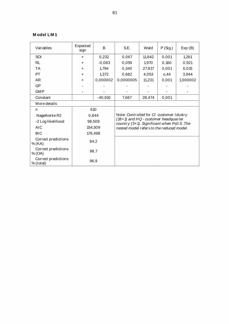
81
Model LM1
Variables Expectedsign B S.E. Wald P (Sig.) Exp (B)
SOI + 0,232 0,067 11,842 0,001 1,261RL + -0,083 0,059 1,970 0,160 0,921TA + 1,794 0,340 27,817 0,001 6,015PT + 1,372 0,682 4,053 o,44 3,944AR + 0,000002 0,0000005 11,231 0,001 1,000002GP - - - - - -GMP - - - - - -Constant -40,910 7,667 28,474 0,001More detailsn 610
Note: Controlled for CI customer Idustry(18+1) and HQ - customer headquartercountry (3+1). Significant when P 0.5. Thenested model refers to the reduced model.
Nagelkerke R2 0,844-2 Log likelihood 98,509AIC 154,509BIC 176,498Correct predictions
% (KA) 84,2
Correct predictions% (OA) 98,7
Correct predictions% (total) 96,9

82
Model LM2
Variables Expectedsign B S.E. Wald P (Sig.) Exp (B)
SOI + 0,243 0,068 12,924 0,001 1,275RL + -0,063 0,055 1,336 0,248 0,939TA + 1,680 0,297 32,088 0,001 5,363PT + 1,230 0,638 3,556 0,59 3,33AR - - - - - -GP + 0,000003 0,000001 6,845 0,001 1,000003GMP - - - - - -Constant -38,439 6,079 32,827 0,001More detailsn 610
Note: Controlled for CI customer Idustry (18+1)and HQ - customer headquarter country (3+1).Significant when P 0.5. The nested model refersto the reduced model.
Nagelkerke R2 0,832-2 Log likelihood 105,539AIC 161,539BIC 183,528Correct predictions
% (KA) 80,3
Correct predictions% (OA) 98,5
Correct predictions% (total) 96,2

83
Model LM3
Variables Expectedsign B S.E. Wald P (Sig.) Exp (B)
SOI + 0,359 0,062 33,007 0,001 1,431RL + -0,052 0,057 0,848 0,357 0,949TA + 1,539 0,246 39,129 0,001 4,661PT + 1,068 0,594 3,227 0,72 2,909AR - - - - - -GP - - - - - -GMP + -0,11 0,007 2,285 0,131 0,989Constant -35,085 5,574 39,626 0,001More detailsn 610
Note: Controlled for CI customer Idustry(18+1) and HQ - customer headquartercountry (3+1). Significant when P 0.5. Thenested model refers to the reduced model.
Nagelkerke R2 0,822-2 Log likelihood 110,733AIC 166,733BIC 188,722Correct predictions
% (KA) 82,9
Correct predictions% (OA) 98,5
Correct predictions% (total) 96,6

84
APPENDIX 2
Model summary LS, LS1, LS2, LS3
VariablesLS (CI and HQ) LS1 (+ AR) LS2 (+ GMU) LS3 (+ GMP)
Exp (B) P (Sig.) Exp (B) P (Sig.) Exp (B) P (Sig.) Exp (B) P (Sig.)
AR - - 1,000002 0,001 - - - -GP - - - - 1,000005 0,001 - -GMP - - - - - - 0,998 0,750
n 610 610 610 610 Nagelkerke R2 0,265 0,615 0,576 0,266-2 Log likelihood 366,51 218,663 237,135 366,372AIC 412,51 266,663 285,135 414,372BIC 430,573 285,511 303,983 433,220LRT (Chi2 d) Nested 147,847 129,375 0,140LRT (Sig.) Nested 0,001 0,001 0,710Correct predictions
% (KA) 9,2 57,9 56,6 9,2
Correct predictions% (OA) 99,3 99,3 99,3 99,3
Correct predictions% (total) 88,0 94,1 93,9 88,0
Note: Controlled for CI: customer Idustry (18+1) and HQ: customer headquarter country (3+1).Significant when P 0.5. The nested model refers to the reduced model.

85
Model summary LS4, LS5, LS6, LS7
VariablesLS4 (+ OI) LS5 (+ RL) LS6 (+ TA) LS7 (+PT)
Exp (B) P (Sig.) Exp (B) P (Sig.) Exp (B) P (Sig.) Exp (B) P (Sig.)
SOI 1,514 0,001 - - - - - -RL - - 1,033 0,181 - - - -TA - - - - 4,419 0,001 - -PT - - - - - - 3,539 0,001
n 610 610 610 610 Nagelkerke R2 0,623 0,270 0,703 0,312-2 Log likelihood 215,160 364,712 175,079 348,641AIC 263,160 412,712 223,079 396,641BIC 282,008 431,560 241,927 415,489LRT (Chi2 d) 151,35 1,798 191,431 17,869LRT (Sig.) 0,001 0,180 0,001 0,001Correct predictions
% (KA) 55,3 9,2 71,1 7,9
Correct predictions% (OA) 98,1 99,3 97,8 99,4
Correct predictions% (total) 92,8 88,0 94,4 88,0
Note: Controlled for CI: customer Idustry (18+1) and HQ: customer headquarter country (3+1).Significant when P 0.5. The nested model refers to the reduced model.


