Profitable Momentum Trading Strategies for Individual Investors Bryan Foltice, Thomas Langer * Finance Center Münster, University of Münster, 48143 Münster, Germany Abstract For nearly three decades, scientific studies have explored momentum investing strategies and observed stable excess returns in various financial markets. However, the trading strategies typically analyzed in such research are not accessible to individual investors due to short selling constraints, nor are they profitable due to high trading costs. Incorporating these constraints, we explore a simplified momentum trading strategy that only exploits excess returns from topside momentum for a small number of individual stocks. Building on US data from the New York Stock Exchange from July 1991 to December 2010, we analyze whether such a simplified momentum strategy outperforms the benchmark after factoring in realistic transaction costs and risks. We find that the strategy can indeed work for individual investors with initial investment amounts of at least $5,000. In further attempts to improve this practical trading strategy, we analyze an overlapping momentum trading strategy consisting of a more frequent trading of a smaller number of “winner” stocks. We find that increasing the trading frequency initially increases the risk-adjusted returns of these portfolios up to an optimal point, after which excessive transaction costs begin to dominate the scene. In a calibration study, we find that, depending on the initial investment amount of the portfolio, the optimal momentum trading frequency ranges from bi-yearly to monthly. JEL Classifications: G11, G12, G14 Keywords: Momentum Investing, Personal Finance, Portfolio Management Bryan Foltice - University of Münster, Münster, Germany - Email: [email protected]Thomas Langer - University of Münster, Münster, Germany - Email: [email protected]1
Transcript
Profitable Momentum Trading Strategies for Individual Investors
Bryan Foltice, Thomas Langer* Finance Center Münster, University of Münster, 48143 Münster, Germany
Abstract
For nearly three decades, scientific studies have explored momentum investing strategies and observed stable excess returns in various financial markets. However, the trading strategies typically analyzed in such research are not accessible to individual investors due to short selling constraints, nor are they profitable due to high trading costs. Incorporating these constraints, we explore a simplified momentum trading strategy that only exploits excess returns from topside momentum for a small number of individual stocks. Building on US data from the New York Stock Exchange from July 1991 to December 2010, we analyze whether such a simplified momentum strategy outperforms the benchmark after factoring in realistic transaction costs and risks. We find that the strategy can indeed work for individual investors with initial investment amounts of at least $5,000. In further attempts to improve this practical trading strategy, we analyze an overlapping momentum trading strategy consisting of a more frequent trading of a smaller number of “winner” stocks. We find that increasing the trading frequency initially increases the risk-adjusted returns of these portfolios up to an optimal point, after which excessive transaction costs begin to dominate the scene. In a calibration study, we find that, depending on the initial investment amount of the portfolio, the optimal momentum trading frequency ranges from bi-yearly to monthly.
JEL Classifications: G11, G12, G14
Keywords: Momentum Investing, Personal Finance, Portfolio Management
Bryan Foltice - University of Münster, Münster, Germany - Email: [email protected] Thomas Langer - University of Münster, Münster, Germany - Email: [email protected]
Researchers have been writing about momentum trading since the 1990s. In their original
work, Jegadeesh and Titman (1993) found that buying (shorting) the 10% best (worst)
performing stocks from the previous 3, 6, 9, and 12 months can result in abnormal profits of
approximately 1% per month after holding each portfolio for 3, 6, 9, or 12 months. Other
empirical research finds the same results in various markets around the world with
Rouwenhorst (1998) finding profits in 12 European countries, profits in emerging markets
(Cakici, Fabozzi, & Tan, 2013; Rouwenhorst, 1999), and positive returns in 31 of 39
international markets (Griffin, Ji, & Martin, 2003). Asness, Moskowitz, and Pedersen (2013)
evaluate momentum jointly across eight various markets and find consistent momentum
return premia across all evaluated markets. Fama and French’s three-factor model (1993)
cannot sufficiently explain the continuation of short-term returns found in the United States
(Jegadeesh & Titman, 1993; 2001). They later describe the abnormal returns yielded by
momentum strategies as the “premiere anomaly” of their three-factor model (Fama & French,
2008). Unfortunately for individual investors, momentum investing, as originally outlined by
Jegadeesh and Titman (1993), assumes a zero-cost trading strategy, which omits various
market frictions, such as transaction costs, bid-ask spreads, and short-selling constraints.
Carhart (1997) concludes that momentum trading, as proposed by Jegadeesh and Titman
(1993), becomes unprofitable after factoring in such trading costs.
Although the theory of momentum investing is well documented in literature, the body of
applied research as it pertains to individual investors is relatively small. Rey and Schmid
(2007) use Swiss data to show that investors could earn profits up to 44% annually by buying
the top performer in the SMI and selling short the worst performer in the same formation
period. In the US market, Ammann, Moellenbeck, and Schmid (2011) find significant
abnormal monthly returns of 1.16% to 2.05% by buying the single best performing stock in
2
the S&P 100 and shorting the index. Additionally, Siganos (2010) concedes that it would be
too costly for retail investors “to buy/sell short hundreds of stocks” and employs U.K. data for
the top and bottom 1-50 best and worst performers. Siganos concludes that after accounting
for transaction costs and risk that small investors (with portfolios ranging from £5,000 to
£1,000,000) can exploit the momentum effect with only a limited number of stocks.
Furthermore, this work finds evidence that momentum profits increase as the number of
stocks in the portfolio decreases (Siganos, 2007).
These works lay an encouraging foundation for small investors and a solid framework for our
analysis. However, these papers imply that private investors have the capability to short
stocks in their portfolio.1 Momentum trading, as proposed by previous literature, exposes
investors to unlimited downside risk by short selling uncovered positions in their portfolios.
Moreover, private investors would have to contend with additional “hard to borrow” fees.2
Margin risk is also something that accompanies short selling and should be only engaged by
very knowledgeable investors who understand the risks involved.3 Thus, this paper examines
the feasibility of private investors profiting from buying long only the “winner” portfolio.4
Individual investors do not have many opportunities to consistently outperform the
benchmark. Research shows that in the nearly $12 trillion mutual fund industry, only 0.6% of
all mutual funds outperformed the benchmark after accounting for risks, expenses, and
management fees (Wermers, Barras, & Scaillet, 2010). Even if mutual funds that beat the
benchmark exist, the question remains: How would an individual investor choose the correct
1 Although it is unclear how many investors have the option to short stocks in their account, Barber and Odean (2009) show that only 0.29% of all individual investors took short positions in their portfolio. 2 If a customer has shorted a stock, the clearing firm has to borrow it in order to deliver it to the buyer. When there is a huge demand to short a stock and there is a shortage of shares to borrow, holders of long stock can charge potentially very high rates to borrow stock. 3 Margin requirements for small and microcap stocks are often much higher than the standard 30-50% margin requirement. 4 According to Jegadeesh and Titman’s (1993) and Grinblatt and Moskowitz’s (2004) findings, the abnormal performance of momentum trading is mainly due to the winner portfolio rather than the loser portfolio.
3
over performing mutual fund? Answering this question is far beyond most individual
investor’s capacity.
Recently, a handful of mutual funds based on the momentum effect have become available to
individual investors. The most notable mutual fund family that uses stock price momentum is
AQR Capital Management. The Momentum Fund (Symbol AMOMX), started in 2009, is the
largest AQR fund, with assets of nearly $1 billion. According to the fund’s website, the
portfolio is rebalanced at least quarterly (AQR Funds, 2011) and management always buys
the top one-third of the best performing stocks on the Russell 1000 Index (which also
incorporates the “buying the winners only” strategy), based on the returns of the previous 12
months. Unfortunately, this fund currently has a high entry barrier for individual investors,
seeing that it requires a minimum initial investment of $5,000,000.
The good news for individual investors about momentum trading is that the strategy requires
very little knowledge of investing (Siganos, 2010) and only a small time commitment to
research the previous winners, which can easily be done on the Internet. According to
Goetzmann and Kumar (2008), 79.99% of all the households in their analysis traded
individual stocks at least once. Moreover, today’s trading environment allows investors to
trade stocks in their accounts for less cost.5 Investors can now choose which type of buy
(market orders, on the open, on the close) and sell orders (stop loss, trailing stop loss) they
would like at the beginning and end of each holding period.6 Finally, all investors have the
option to “reinvest all dividends” at no additional cost when they buy stocks, eliminating the
cost of holding cash earned on dividends. The details on how and when individuals can easily
execute this strategy at the beginning and end of each holding period are outlined in the data
and methodology section.
5 As of June 16, 2011 the costs of trading a stock averaged $8.77 per trade at five of the largest US discount brokers (Fidelity $7.95, Schwab $8.95, Scott Trade $7, E-Trade $9.95, TD Ameritrade $9.99). 6 On the first day of the holding period, investors can place “good ‘til canceled” stop loss or trailing stop orders for an amount or percentage loss that remain open up to 120 days.
4
The remainder of this paper analyzes the momentum returns of the top performing 1-50 stocks
traded on the New York Stock Exchange from July 1, 1991 to December 31, 2010 and finds
numerous opportunities for individual investors, with initial investments ranging from $5,000
to $1,000,000, to outperform the benchmark after accounting for transaction costs and risk.
This is not the first paper to investigate the profit potential of momentum trading for
individual investors after factoring in costs and risks. However, after investigating the initial
gross momentum returns, we notice higher returns in the smaller portfolios, that is, those with
fewer than 10 stocks, coupled with higher portfolio volatility. Based on this finding, this paper
adds to the current body of literature by introducing increased momentum trading frequencies
in order to reduce the volatility of the portfolio returns while capturing the higher average
returns possible in the portfolios consisting of a small number of “winner” stocks. The trade-
off between the reduced volatility of these returns and the reduced portfolio performance due
to the higher transaction costs is evaluated. We find evidence that buying the smaller
overlapping portfolios consisting of the top five to eight best performers of the six-month
formation period on a bi-yearly to monthly basis results in larger risk-adjusted returns
compared to buying a larger portfolio consisting of 20-50 stocks one time per year. We
conclude that each initial investment amount has a different optimal trading frequency, the
point yielding the highest Sharpe ratio against the benchmark, at which the trade-off is the
greatest, ranging from bi-yearly to monthly trading.
2. Data and Methodology
For this analysis, all equities traded on the New York Stock Exchange (NYSE) as of
November 23, 2011 were included in the original data set. All stock information was collected
from July 1, 1991 to December 31, 2010 using Thomson Reuters Datastream. Both delisted
and active NYSE stocks were included in this sample to avoid any survivorship bias. The total
number of stocks in our original sample ranged from 1,786 to 3,121 with an average of 2,286
5
stocks each month. All stocks were included in the initial analysis, even those that traded for
less than $5. However, for the analysis highlighted in this paper, we eliminated all stocks with
a market capitalization (MV in Datastream) less than $20 million on the first day of the
holding period. This filter primarily eliminates the potentially illiquid stocks that have
extremely high bid and ask spreads. It also prevents an individual with a million dollar
portfolio from potentially owning over 5% of all outstanding shares, thus avoiding the need to
file Schedule 13D with the Securities and Exchange Commission (SEC).7 Adding this filter
slightly decreases the overall gross returns of each portfolio, though it does not have a
significant impact on the overall results. After applying the market capitalization filter, the
size of the data set is an average of 2,102 stocks per month, with a range of 1,722 to 2,589.
For the analysis, a six-month formation period (-5 to 0 months) is implemented, using the
daily closing prices of each stock on the first trading day in the formation period and the last
trading day of the formation period. For example, the formation period starting in February
would run from the closing stock prices on February 1 to the closing prices on July 31,
providing both were valid trading days. Each stock would be ranked by its formation period
(six-month) performance, from best to worst.8 The total return (RI in Datastream) for each
stock was used in order to fully reflect dividends.9 After ranking each stock, equally weighted
portfolios were formed that contained the best (1, 2, 3, 4, 5, 6, 7, 8, 9, 10, 15, 20, 30, 40, 50)
performing stocks in the formation period.
We established a 12-month holding period and bought each stock at the closing price on the
first trading day of the period. At the end of the 12-month holding period, all stocks were sold
7 When a person or group of persons acquires beneficial ownership of more than 5% of a voting class of a company’s equity securities registered under Section 12 of the Securities Exchange Act of 1934, they are required to file a Schedule 13D with the SEC. Viewed on 08.04.2014. http://www.sec.gov/answers/sched13.htm 8 Companies that become delisted during the formation period were assigned a return of 0%, which is consistent with Agyei-Ampomah (2007) and Siganos (2010). However, no delisted stocks made it into any of the winner portfolios during the analyzed period. 9 As previously mentioned, investors can opt to fully reinvest dividends when buying each stock. This is a free service at most discount brokers in the United States.
6
at the closing price on the last trading day of the period. For example, the holding period
would begin at the closing price on August 1 and all stocks would be held until the closing
price on July 31 the following year (given that both are valid trading days). The intuition
behind this is that individuals realistically would be able to turnover their portfolio in one
sitting. For instance, an investor could place “sell at the close” orders on the last day of the
holding period, calculate previous returns of the formation period after the market closes, and
set up his or her trades using the proceeds from the sales to place “buy at the close” orders on
the next trading day.10 Proceeds from sold stocks are immediately available to purchase new
stocks at most discount brokers, thus avoiding the otherwise T+3 settlement days for funds to
become available.
The overall return of each time period was calculated by averaging the performance of all
stocks in each portfolio. Over multiple time periods, the average annual total return
(geometric mean) of each portfolio was calculated in order to reach the gross returns, as
prescribed by the SEC for all U.S. mutual funds.11 Later in our analysis, these returns and
their respective trading costs were applied to nine different portfolio sizes with initial
investments ranging from $5,000 to $1,000,000. The returns after all applicable transaction
costs are applied are shown in the risk analysis section.
3. Empirical Findings
3.1 Gross Returns
For gross returns unadjusted for costs, we calculate the overall performance of each portfolio
from holding periods starting in January 1992 and lasting until December 2010.
10 Investors in the United States can set up “buy at the close” and “sell at the close” orders for no additional charge. 11 SEC website viewed 08.02.2012 http://www.sec.gov/rules/final/33-7512f.htm#E12E2
7
Table 1: Gross Momentum Returns, Unadjusted for Costs (% per Month)
Portfolio Size 8 9 10 15 20 30 40 50 Jan 1992-Dec 2010 3.06*** 2.91*** 2.82*** 2.54*** 2.36*** 2.28*** 2.20*** 2.13*** Max 23.50 23.72 21.27 16.80 13.94 11.13 10.41 9.70 Min -6.20 -5.94 -5.83 -5.73 -5.53 -5.07 -5.18 -4.85 Median 3.40 3.53 3.32 3.08 3.04 2.85 2.76 2.76 Monthly St Dev. 0.19 0.18 0.17 0.14 0.12 0.11 0.10 0.10 Correlation 0.43 0.45 0.46 0.51 0.55 0.62 0.64 0.65 Outperform SP500 74% 74% 75% 73% 76% 78% 78% 77% Sub-periods 1992-2000 3.36 3.20 3.08 2.72 2.52 2.60 2.54 2.53 2001-2009 2.77 2.64 2.57 2.36 2.21 1.97 1.88 1.74 2007-2008 -2.81 -2.70 -2.71 -2.42 -2.17 -2.06 -2.12 -2.12 1992-2006; 09-10 4.14 3.93 3.81 3.40 3.12 3.00 2.92 2.83 Note: For the analysis, a six-month formation period (-5 to 0 months) is implemented, ranking each stock by its formation period (six-month) performance, from best to worst. After ranking each stock, equally weighted portfolios were formed that contained the best (1, 2, 3, 4, 5, 6, 7, 8, 9, 10, 15, 20, 30, 40, 50) performing stocks in the formation period. We established a 12-month holding period and the overall return of each time period was calculated by averaging the performance of all stocks in each portfolio. Over multiple time periods, the average annual total return (geometric mean) of each portfolio was calculated in order to reach the monthly gross returns. Correlation is between each portfolio and the S&P 500. "Outperform S&P 500" means the percentage of months where each portfolio outperforms the S&P 500 benchmark. Statistical significance of the overall returns is given by two sample parametric t-tests comparing the returns of each portfolio with the S&P 500. * Significant at the 10% level, ** significant at the 5% level, *** significant at the 1% level.
The results in Table 1 show that all portfolios, on average, outperform the S&P 500
benchmark by 0.52%-2.44% per month.12 Consistent with Siganos (2007), larger momentum
profits were primarily seen in the smaller portfolios. However, the portfolio containing the
12 The S&P 500 was used as the benchmark in this analysis as it the most commonly used benchmark for U.S. stocks. We also ran the risk analysis against the Willshire 5000 Index, arguably a more comparable benchmark, and found similar results.
8
best performing stock performed the worst out of all portfolios (1.15%), which is inconsistent
with the findings of Ammann, Moellenback, and Schmid (2011) and with those of Rey and
Schmid (2007). Overall portfolio performance gradually increases until it reaches the highest
performance, 3.07% per month, in the top seven stock portfolio. The returns then decrease as
the portfolio holds more stocks. Regardless, the top 50 stock portfolio still outperformed the
S&P 500 by 1.50% per month in the overall sample period.
Gross returns were divided into two equal sub-periods, January 1992 to December 2000 and
January 2001 to December 2009. Each sub-period appears to consistently outperform the S&P
500 in both categories. However, momentum trading clearly struggled during the financial
crisis of 2007 and 2008, incurring heavy losses and faring much worse than the S&P 500. In
this period, all portfolios underperformed the S&P 500 by 0.54% in the top 50 portfolio, and
by as much as 2.74% per month in the one stock portfolio. These findings are consistent with
Andrikopoulos, Clunie, and Siganos (2013), who find no evidence of momentum returns
during a similar period, February 2007 to February 2010, in the U.K. market. In hindsight, it
would have been more profitable to either stay in cash or seek an alternative trading
strategy.13 We hope that these findings inspire further research into whether it is possible to
capture reliable ex-ante cues from the formation period data that can inform investors as to
whether they should continue with the momentum strategy or opt for an alternative trading
strategy for those holding periods.
3.2 Transaction Costs
To more accurately analyze the true profitability of momentum trading, all applicable
transaction costs are applied to each portfolio. At the beginning and end of each holding
period, a flat $10 commission per trade was factored in for each buy and sell order.
13 Daniel and Moskowitz (2013) find that in extreme market environments, the loser portfolio provides a high premium, while the winner portfolio returns are minimal following large market declines.
9
The bid and ask spreads were also taken into account for each stock. The actual bid and ask
spreads for the stocks were available only from April 2006 to December 2010. Therefore, we
implemented averaged bid and ask spreads based on the market capitalization of each stock,
using the bid/ask spread averages from small, mid, and large cap stocks listed on the NYSE in
1998 (Bessimbinder, 2003). Specifically, for all stocks with a market capitalization under
$215.6 million we assume a 0.750% half spread on both the buy and sell order each period. A
half spread of 0.497% was used for stocks with market capitalization between $215.7 and
$11,365.8 million. All stocks with a market capitalization greater than $11,365.8 million were
given a half spread of 0.212%.14 For the top 50 performers over the 18-year sample period,
31% of the stocks were classified as small capitalization, 65% were mid-capitalization, and
4% were large capitalization. Although the lack of actual bid and ask data was not ideal, the
current market is so heavily traded that every stock ranked in the top 10 best performing
stocks for all 12 formation periods in 2010 had an average bid and ask spread of $.01,
providing a more favorable trading environment for investors seeking to implement this
strategy in the future.
Finally, a nominal “Securities and Exchange Commission (SEC) Fee” for every sale of a
stock was included at its rate, prior to December 28, 2001, 0.003333% of the total amount
sold.15
14 These assumptions are supported by the available bid/ask spread data from April 2006 to December 2010. During this time span, the average actual small cap stock posted a half bid/ask spread of 0.65%, which is slightly less than our assumed average. The mid cap and large cap stocks posted significantly lower actual bid/ask half spreads, 0.19% and 0.10%, respectively. As a robustness check, we ran the analysis with the actual spreads of the relevant stocks for this period and found no systematic difference from the results in our base scenario with fixed spreads for small, mid, and large caps. 15 Section 31 of the Securities Exchange Act of 1934 states that, “self-regulatory organizations (SROs) such as the Financial Industry Regulatory Authority (FINRA) and all of the national securities exchanges (including the New York Stock Exchange) must pay transaction fees to the SEC based on the volume of securities sold on their markets. These fees recover the costs incurred by the government, including the SEC, for supervising and regulating the securities markets and securities professionals.” Viewed on 05.03.2014 on at http://www.sec.gov/answers/sec31.htm.
10
To maintain an equally weighted portfolio at the beginning of each holding period, all
portfolios were rebalanced at the end of the previous holding period. Therefore, at the end of
the holding period, the full $10 commission for each stock, the other half bid/ask spread, and
the SEC selling fee were added to the full amount of the sell order of each stock. In summary,
the overall costs, o, to implement a 12-month momentum strategy are:
𝑜𝑜 = (2 ∗ 𝑐𝑐) + (2 ∗ 0.5𝑠𝑠) + 𝑓𝑓 (1)
Where c is the sales commission, s is the bid/ask spread, and f is the SEC sales fee.
These transaction costs are applied to nine different initial investment amounts ranging from
$5,000 up to $1,000,000 in order to reflect the feasibility and effects on performance.
Table 2 shows the net monthly returns after applying transaction costs. With a trading
frequency of only once per year, all (except one) portfolios continued to outperform the S&P
500.16 Yearly traded portfolios containing the top five to eight stocks continue to generate the
highest gross returns, ranging from 2.66% to 2.96% per month. No expenses were added to
the S&P 500 benchmark in this section, which further strengthens the results.
16 The top 50 stock portfolio with an initial amount of $5,000 underperformed the S&P 500 by 0.39% per month.
11
Table 2: Net Monthly Momentum Returns After Adding Transaction Costs (%) Full Turnover; Yearly Trading Frequency S&P 500 Return: 0.63
Note: Full turnover applies the commission ($10 per stock) and half bid/ask spread at the beginning of each holding period. At the end of the holding period, the full turnover applies the full commission for each stock, the other half bid/ask spread and the SEC selling fee on the full amount of the sell order of each stock. Statistical significance is given by two sample parametric t-tests comparing the returns of each portfolio with the S&P 500.
* Significant at the 10% level, ** significant at the 5% level, *** significant at the 1% level.
12
3.3 Real Turnover
It is possible that, when turning over the portfolio from one holding period to the next, an
individual stock could remain in the portfolio. In this case, the overall portfolio would still
need to be rebalanced, requiring a buy or sell order for a fraction of this stock position, in
order to maintain an equally weighted portfolio at the beginning of each holding period. Thus,
one $10 commission would still be applied for each stock. However, the second commission
of $10 is saved in this instance as only one transaction is needed for the adjustment.
Moreover, as only a fraction of the stock position would be bought or sold for rebalancing
purposes, the negative consequences of the bid/ask spread are mostly waived, thereby further
reducing the overall transaction fees. We make these adjustments so as to reflect the real-
world situation as accurately as possible, even though comparing Table 3 (real turnover) with
Table 2 (full turnover) shows that the performance effect is negligible. Nevertheless, we
consider the real turnover in all analyses that follow.
13
Table 3: Net Monthly Momentum Returns After Adding Transaction Costs (%) Real Turnover; Yearly Trading Frequency S&P 500 Return: 0.63
$1,000,000 1.12 2.61*** 2.84*** 2.84*** 2.94*** 2.94*** 2.97*** 2.96*** 2.82*** 2.72*** 2.44*** 2.27*** 2.18*** 2.11*** 2.03*** Note: Net monthly momentum returns, reflecting the real portfolio returns for those stocks remaining in each portfolio from one holding period to the next. Thus, a commission of $10 is saved in this instance as a new stock is not required to be purchased for the next holding period. Moreover, as only a fraction of the stock holding would be sold for rebalancing purposes, the negative consequences of the bid/ask spread would be waived, thereby further reducing the overall transaction fees. Statistical significance is given by two sample parametric t-tests comparing the returns of each portfolio with the S&P 500. * Significant at the 10% level, ** significant at the 5% level, *** significant at the 1% level.
14
3.4 Risk Factors
This section applies the net monthly results from the previous section to various risk factors in
order to determine if these returns continue to outperform the benchmark after factoring in
risk. The capital asset pricing model (Sharpe, 1964) and the Fama-French three factor model
(1993) are applied to the net monthly returns of each portfolio in order to test against
systematic risk.
For the capital asset pricing model (CAPM), overlapping data were used in the sample set. A
majority of recent finance literature employs overlapping data (Harri & Brorsen, 2009),
although there is no consensus on which type of data are less biased. To control for the
autocorrelation of the overlapping data, the Newey-West (1987) estimator with an 11-month
lag was applied. For our estimation, we use the following equation:
𝑁𝑁𝑁𝑁 − 𝑅𝑅𝑓𝑓 = β ( 𝐾𝐾𝑚𝑚 − 𝑅𝑅𝑓𝑓 ) + α (2)
where “𝑅𝑅𝑓𝑓” is the risk free rate from French’s Data Library, “𝑁𝑁𝑁𝑁” is the net monthly return,
and “𝐾𝐾𝑚𝑚” is the performance of the S&P 500.
For the Fama-French three factor model, we use the following regression:
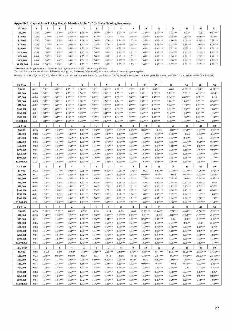
* 10% statistical significance, ** 5% statistical significance, *** 1% statistical significance To control for the autocorrelation of the overlapping data, the Newey-West (1987) estimator with an 11-month lag was applied. We use: Nr - Rf = β(Km - Rf) + α, where "Rf" is the risk free rate from French’s Data Library, "Nr" is the net monthly real turnover portfolio returns, and "Km" is the performance of the S&P 500.
For the Fama-French three factor model, the following regression was used: Nr-Rf= β(Km-Rf )+bs*SMB+ bv*HML+ α, where "Rf" is the yearly risk-free rate, high minus low book to market ratio (HML) and small minus big (SMB) data are from Kenneth French’s Data Library. Similar to the capital asset pricing model, we use "Nr" to signify the net monthly real turnover portfolio returns and "Km" to signify the performance of the S&P 500. Monthly Alpha "α"
Tables 1 to 3 show that noticeably higher average returns were observed in the smaller
portfolios consisting of the top two to ten stocks, compared to the portfolios with 15 to 50
stocks. However, these increased returns coincide with a higher variance of returns. To
reduce the volatility of the portfolio returns, the remainder of the analysis applies six different
trading frequencies for each portfolio, varying from once per year up to monthly. This
strategy was implemented in order to investigate whether the additional trading frequencies
could decrease the volatility of the portfolio returns, while maintaining the larger returns seen
in the smaller portfolios after factoring in transaction costs. In addition to the once per year
strategy, we explore bi-yearly, tri-yearly, quarterly, bi-monthly, and monthly trading
frequencies in order to observe the effects of each trading frequency on their respective
portfolios.
An investor trying to decide how much he should buy of each stock when using an
overlapping strategy would first need to equally divide his initial investment by the number of
times he wants to trade each year, that is, his trading frequency. Then, he would equally
divide that amount by the number of stocks he would like in his portfolio. The equation of
buying power, BP, for each stock in dollars, is:
𝑆𝑆𝐵𝐵 = (𝐴𝐴/ 𝑡𝑡) / 𝑘𝑘 (4)
Where A is the initial investment amount, k is the number of stocks in the portfolio, and t is
the trading frequency per year.
For example, if an investor with an initial investment amount of $50,000 would like to buy
the top five stocks on a quarterly frequency, he would have a buying power of $2,500 for each
stock in the portfolio. Hypothetically, this investor would initially buy $12,500 ($2,500 of
each of the top five performing stocks of the previous six months) on January 1 and hold these
19
stocks until December 31. He would repeat the process on April 1, July 1, and October 1 and
hold the respective portfolios for 12 months (thus selling on March 31, June 30, and
September 30, respectively). In the following year, he would sell each portfolio at the end of
each quarter and use the proceeds to buy the new portfolio. Once the strategy is fully
established, this individual will have up to 20 different stocks in his portfolio at any given
time.17
This increase in stock holdings reduces the volatility of the overall portfolio returns while
enabling the investor to continue to enjoy the higher returns generated by the top five
performing stock portfolio.18 On the other hand, the increased trading frequency dramatically
increases trading costs. In the following sections, we analyze whether the benefits of
decreased volatility, particularly in the smaller portfolios, outweigh the negative effects of
these increased trading costs.
The effects of trading frequency on net monthly performance of the portfolio largely depends
on the initial amount in the portfolio. Unsurprisingly, portfolios with a $5,000 initial
investment were affected the most by the increased trading frequency, while the million dollar
portfolios were barely affected, decreasing from 2.96% per month traded yearly to 2.95%
traded monthly. As the trading frequency increases, the best performing portfolios remain in
the top five to eight stocks for all portfolios with an initial amount of $100,000 or more. The
smaller portfolios, which are more affected by the extra trading costs, post the highest
performance in the smaller (top two to five) stock portfolios as frequency increases. Figure 1
shows an example of the effects of various frequencies on net returns in a portfolio with an
initial investment of $15,000. The effects for all portfolios can be found in Appendix 1.
17 On the other hand, the investor could theoretically have a minimum of five different stocks in the portfolio at any given time, if the same top performers remain in the “winner portfolio” each quarter. 18 This strategy would be compared to buying the top 20 performing stocks once a year.
20
Figure 1: Net Monthly Momentum Returns After Transaction Costs (%) Real Turnover Returns Based on Various Trading Frequencies. This figure shows the returns of a portfolio with an initial value of $15,000. The remaining initial portfolio amounts can be found in Appendix 1.
Next, we again apply the CAPM and Fama-French three-factor model to all trading
frequencies in order to examine the effects on the monthly alphas. Appendices 2 and 3 show
the monthly alphas in the CAPM and the Fama-French three-factor model for each trading
frequency. There are some slight decreases in alpha as the trading frequency increases.
However, most of these strategies maintain a statistically significant positive alpha.
Up to this point in the analysis, we have observed that excess returns exist in many of these
portfolios after factoring in costs and systematic risk. However, most individual investors are
less concerned with beta risk than they are with volatility risk. We maintain that increasing
trading frequencies will decrease the volatility of the returns as well as the idiosyncratic risk
of the portfolio. Therefore, this section determines the optimal trading frequency for each
initial investment amount based on the highest abnormal Sharpe ratio compared to the
To analyze idiosyncratic risks, Sharpe ratios for each portfolio were computed and compared
against the benchmark’s Sharpe ratio in order to determine the optimal trading frequency for
each initial portfolio amount. The Sharpe ratio equation is:
𝑆𝑆ℎ𝑎𝑎𝑁𝑁𝑎𝑎𝑎𝑎𝑖𝑖 = 𝑁𝑁𝑁𝑁𝑖𝑖−𝑅𝑅𝑓𝑓𝜎𝜎𝑖𝑖
(5)
using the aforementioned net monthly real turnover returns “Nr”, “Rf” as the risk free rate,
and “σ” as the standard deviation of the portfolio returns.
Figure 2: Abnormal Monthly Sharpe Ratios Compared to the S&P 500 Benchmark. This figure shows the abnormal ratios of a portfolio with an initial value of $30,000 for different trading frequencies.
Figure 2 displays the abnormal monthly Sharpe ratios for each trading frequency compared to
the S&P 500 benchmark for a portfolio with an initial value of $30,000.19 The results indicate
that for all initial investment amounts with portfolios containing the top four to ten best
performing stocks, the abnormal Sharpe ratio increases as the trading frequency increases
(statistically significantly) from yearly to bi-yearly.20 This provides some initial evidence that
19 Again, replacing the S&P 500 with the Willshire 5000 as the benchmark makes no qualitative difference in the analysis. 20 Abnormal Sharpe ratios for all portfolios are displayed in Appendix 4.
Compared to S&P 500 BenchmarkAbnormal Monthly Sharpe Ratios
22
as trading frequency increases, portfolio volatility decreases at a faster pace than performance.
At this point, the abnormal Sharpe ratios reach a peak and then begin to fall as the higher
transaction costs reduce performance at a faster rate than the rate of volatility reduction.
Therefore, the optimal trading frequency is largely dependent on the initial investment
amount. For example, abnormal Sharpe ratios for smaller initial investments of $10,000 and
$15,000 begin to decrease more quickly (between tri-yearly and quarterly trading), while
abnormal Sharpe ratios continue to increase up to monthly trading for the larger initial
investments of $250,000, $500,000, and $1,000,000. In robustness tests, we find similar
patterns in both sub-periods for all initial investment amounts.21
Table 6 outlines the optimal trading frequency for each initial investment amount based on the
highest statistically significant abnormal Sharpe ratios for the top five to eight performing
stock portfolio. It is worth noting that all portfolios have a positive and statistically significant
monthly alpha in the CAPM and Fama-French three-factor model. With the exception of only
a small overlap of CAPM and Fama-French alphas in the $5,000 portfolio, we find evidence
in all other portfolios analyzed that overlapping portfolios provide higher net returns and
alphas compared to non-overlapping strategies with a similar number of stocks in the
portfolio.
21 These results are not shown, but are available on request. 23
Table 6: Comparing Overlapping Portfolios to the Yearly Trading Strategy, by Initial Portfolio Amount. The frequencies for each portfolio are based on the highest statistically significant abnormal Sharpe ratios of the top five to eight performing stocks.
Overlapping Portfolios Yearly Strategy
Amount Frequency Net Return CAPM α FF3F α Max # Stocks Net Return CAPM α FF3F α
$1,000,000 Monthly 2.92%-2.95% 1.73-1.81 1.79-1.81 60-96 (50) 2.03% 1.20 1.22 * Maximum number of stocks at any given time in a portfolio. The numbers in parentheses are the available portfolio sizes used in this analysis to compare the results of the yearly trading frequency. Net monthly returns of the real turnover portfolios are provided. Note: All CAPM and FF3F α's in this table are significant at the 99% confidence level 5. Conclusion
This paper offers a simplified trading strategy for earning excess returns from top-side
momentum (i.e., buying only previously top performing stocks). Consistent with the U.K.
data employed by Siganos (2010), we find that it is indeed possible for individuals with initial
investment amounts of at least $5,000 to achieve profitability. After factoring in transaction
costs and risks, the highest returns and monthly alphas are obtained by buying the top five to
eight of the top performing stocks of the previous six-month holding period. Furthermore, we
find evidence that volatility decreases at a greater rate than performance as the trading
frequency increases. We conclude that, depending on the initial investment of the portfolio,
the optimal momentum trading frequency ranges from bi-yearly to monthly.
These findings provide a practical solution for individual investors looking for simple trading
strategies that generate excess returns. Moreover, we believe that more work can be done on
this topic, particularly in regard to effective “exit” trading strategies, such as stop losses and
24
trailing stop losses, to achieve higher performance and less volatility, or by combining the
momentum portfolios mentioned in this paper with index funds in order to more optimally
diversify while still benefiting from the abnormal returns and positive alpha of the small
“winner” portfolios.
25
Appendix 1: Net Monthly Momentum Returns After Transaction Costs (%) Real Turnover Returns Based on Various Trading Frequencies and Initial Portfolio Amounts.
* 10% statistical significance, ** 5% statistical significance, *** 1% statistical significance. To control for the autocorrelation of the overlapping data, the Newey-West (1987) estimator with an 11-month lag was applied.
We use: Nr - Rf = β(Km - Rf) + α, where "Rf" is the risk-free rate from French’s Data Library, "Nr" is the net monthly real turnover portfolio returns, and "Km" is the performance of the S&P 500.
* 10% statistical significance, ** 5% statistical significance, *** 1% statistical significance For the Fama French three-factor model, the following regression was used: Nr-Rf= β(Km-Rf )+bs*SMB+ bv*HML+ α, where “Rf” is the yearly risk.free rate. The high minus low book to market ratio (HML)
and small minus big (SMB) data are from Kenneth French’s Data Library. Similar to the capital asset pricing model, we use “Nr” to signify the net monthly real turnover portfolio returns and “Km” to signify the performance of the S&P 500.
Trading Frequency 2X Year 1 2 3 4 5 6 7 8 9 10 15 20 30 40 50
Statistical significance (conventional parametric t-tests) * 90%; ** 95%; *** 99% The Sharpe ratio equation is: Sharpe= (Nr -Rf) /σ. The abnormal monthly Sharpe ratio is the monthly Sharpe ratio of each portfolio minus the monthly Sharpe ratio of the S&P 500 (1992-2010).
29
Acknowledgements
We would like to thank the anonymous referee for the valuable comments on an earlier draft of this
paper. We are also indebted to the participants of the Finance Center Münster econometrics research
seminar at the University of Münster for their helpful comments and insights.
References
Andrikopoulos, P., Clunie, J., & Siganos, A. (2013). Short-selling constraints and
“quantitative” investment strategies. The European Journal of Finance, 19:1, 19-35.
Agyei-Ampomah, S. (2007). The post cost profitability of momentum trading strategies:
Further evidence from the UK. European Financial Management 13, 776-802.
Ammann, M., Moellenbeck, M., & Schmid, M. (2011). Feasible momentum strategies in the
US stock market. Journal of Asset Management, 11, 362-374.
AQR Funds (2011). Momentum Fund Investment Approach. Viewed July 22, 2011 at: