Page 1
PROGRAMME
INFRASTRUCTURES MATERIELLES ET
LOGICIELLES POUR LA SOCIETE
NUMERIQUE – ED. 2011
1/27
Project Acronym CORMORAN (ANR 11-INFR-010)
Document Title
D2.1b - On-Body Antennas Characterization &
Exploitable Radiation Properties – Updated Document : 3D Deterministic Modeling of Electromagnetic Wave Interactions with a
Dielectric Cylinder
Contractual Date of Delivery
None (Extra deliverable)
Actual Date of
Delivery
M22 (10/2013)
Editor UR1
Authors Eric PLOUHINEC
Participants UR1
Related Task(s) T2
Related Sub-Task(s) T2.1
Security Public
Nature Technical Appendix
Version Number 1.0
Total Number of
Pages 27
Page 2
PROGRAMME
INFRASTRUCTURES MATERIELLES ET
LOGICIELLES POUR LA SOCIETE
NUMERIQUE – ED. 2011
2/27
Page 3
PROGRAMME
INFRASTRUCTURES MATERIELLES ET
LOGICIELLES POUR LA SOCIETE
NUMERIQUE – ED. 2011
3/27
TABLE OF CONTENT
D2.1b - On-Body Antennas Characterization & Exploitable Radiation Properties –
Updated Document : 3D Deterministic Modeling of Electromagnetic Wave Interactions with a Dielectric Cylinder 1
TABLE OF CONTENT ............................................................................... 3
ABSTRACT .......................................................................................... 4
EXECUTIVE SUMMARY ............................................................................. 5
1. INTRODUCTION ............................................................................... 6
2. 3D RAY-TRACING ........................................................................... 6
2.1. LOS case ................................................................................................. 7
2.2. NLOS case ............................................................................................... 8
3. INTERACTIONS MODELING WITH UNIFORM THEORY OF DIFFRACTION ................. 9
3.1. Geometrical Optics Formalism .................................................................... 9
3.2. Total Received Field Expression .................................................................. 9
3.2.1 LOS Case 10
3.2.2 NLOS Case 11
3.3. Interaction Coefficients ............................................................................12
3.3.1 Reflection Coefficients 12
3.3.2 Diffraction Coefficients 13
3.4. Special Functions ....................................................................................13
3.4.1 Transition Function 14
3.4.2 Pekeris Function 14
4. MODEL VALIDATION ....................................................................... 15
4.1. 2D validation with literature articles ..........................................................15
4.1.1 Conducting Case 15
4.1.2 Dielectric Case 16
4.2. 3D validation for a Conducting Cylinder Using a Literature Report .................17
5. COMPARISON WITH UR1 SERIES S2 MEASUREMENT CAMPAIGN .................... 19
5.1. Phantom Characteristics ...........................................................................19
5.2. UTD Model Adaptation .............................................................................20
5.3. 2D Comparison .......................................................................................21
5.3.1 For a Distance of 3 cm 21
5.3.2 For a Distance of 9 cm 23
5.3.3 For a Distance of 13 cm 24
6. CONCLUSIONS .............................................................................. 26
7. REFERENCES ................................................................................ 26
Page 4
PROGRAMME
INFRASTRUCTURES MATERIELLES ET
LOGICIELLES POUR LA SOCIETE
NUMERIQUE – ED. 2011
4/27
ABSTRACT
This D2.1 updated document describes an additional work realized for the On-Body
antennas characterization in the CORMORAN project: the deterministic modeling of
electromagnetic wave interactions with a dielectric cylinder. A first additive 3D model
has already been presented in section 5.2 of [Mhedhbi 1] taking into account the
presence of a dielectric cylinder in the immediate proximity of an electromagnetic
source, derived from [McNamara]. But this model only considers the reflection of the
electromagnetic wave with the dielectric cylinder using Geometrical Optics (GO).
Moreover, direct and reflected rays are considered to arrive in the same direction at the
observation point, i.e. the observation point is considered to be far from the cylinder.
Therefore, the phenomenon of “creeping” waves was not considered and there was a
problem when the source and the observation points were in Non Line Of Sight
(NLOS) configuration, i.e. when the observation point was in the shadow region,
because this first model predicted no received field in this configuration. Moreover, the
observation point position was not taken into account. So the idea was to develop a 3D
model able to take into account, not only the reflected wave but also the 2 diffracted (or
“creeping”) waves existing in the shadow region as well as in the lit region. This
prediction model is based on the well-known Uniform Theory of Diffraction (UTD) for
the modeling of the electromagnetic waves interactions and the ray-tracing technique
for the electromagnetic wave paths search. In this updated document of [Mhedhbi 1],
this model is described in details with its major UTD formulations. Then it is validated
in 2D with a conducting and a dielectric cylinder using reference literature articles
[McNamara][Pathak][Hussar]. Concerning the 3D approach, it has been validated with
the measurement of [Govaerts] for a conducting cylinder. Finally it has been compared
with the measurement Series S2 of [Mhedhbi 1], in the 2D configuration, giving results
very close to the measurements.
Page 5
PROGRAMME
INFRASTRUCTURES MATERIELLES ET
LOGICIELLES POUR LA SOCIETE
NUMERIQUE – ED. 2011
5/27
EXECUTIVE SUMMARY
This document presents the additional studies made on the deterministic modeling of
an electromagnetic wave propagation, in presence of a 3D dielectric cylinder. This
model implies 2 steps: first, the search of the electromagnetic wave paths in the lit
(Line Of Sight (LOS) case) and in the shadow (Non Line of Sight (NLOS) case) regions,
using a ray-tracing technique and, secondly, the received field computation using the
Uniform Theory of Diffraction (UTD). The principal novelties, in comparison with the
3D additive model described in [Mhedhbi 1], are the modeling of the diffracted or
“creeping” waves on the cylinder and the observation point position consideration.
First, the ray-tracing technique is described explaining how we find the reflected and
diffracted paths of the electromagnetic wave in 2D as well as in 3D configurations.
Secondly, the UTD principal formulations, allowing the computation of the total
electromagnetic field at the observation point, are presented. Then, the model is
validated in 2D with a conducting [McNamara][Pathak] and a dielectric [Hussar]
cylinder. It is also validated in 3D with a conducting cylinder [Govaerts]. This model
also gives results very close to the measurement series S2 of [Mhedhbi 1] in the 2D
configuration.
Page 6
PROGRAMME
INFRASTRUCTURES MATERIELLES ET
LOGICIELLES POUR LA SOCIETE
NUMERIQUE – ED. 2011
6/27
1. INTRODUCTION
This Document is related to the subtask 2.1 of the CORMORAN project and is an Appendix
of the Technical Report [Mhedhbi 1]. This subtask focused on investigating and modeling the
interaction of the antenna with the body, according to its orientation and proximity.
In this project, the UR1 team is particularly in charge of the WBAN channel modelling. One
possibility is then the deterministic WBAN channel modelling using UTD (Uniform Theory
of Diffraction). UTD allows the received electromagnetic field computation associated with
ray-tracing. This theory is only used with canonical shapes implying that human body could
be modelled by cylinders, which is one of the solutions explored by the CORMORAN Project
for the Channel Modelling. The cylinder could model, for instance, an arm, the trunk or a leg.
In this updated document, a deterministic 3D propagation prediction model is presented,
specific to the electromagnetic wave propagation in the presence of a 3D circular dielectric
cylinder. The used ray-tracing technique and the UTD formulations are detailed. Then, this
model has been validated in 2D with a conducting [McNamara][Pathak] and a dielectric
cylinder [Hussar], and in 3D with a conducting cylinder [Govaerts]. This model is also
particularly compared to the measurement series S2 of the characterization of body-worn
antennas relying on a specific over-the-air (OTA) test-bed in anechoic chamber and a near-
field antenna measurement chamber [Mhedhbi 1].
This document is structured as follows: in Section 2, we describe the specific 3D ray-tracing
used for an electromagnetic source in presence of a circular dielectric cylinder. Then, in
Section 3, the specific UTD formulations, used for the computation of the total received
electromagnetic field, are given. In Section 4, we focus on the validation of the used
theoretical formulations of the model with articles of the literature in 2D (conducting and
dielectric cases) and in 3D (conducting case). Finally, in Section 5, we make a comparison of
this UTD model with measurement series S2 of [Mhedhbi 1] in a 2D configuration.
In this technical Appendix, the UTD deterministic channel modelling is only described for
the “Scattering” case, i.e. Transmitter and Receiver far from the cylinder. Two other cases
could be modelled with UTD:
- “Radiation” case when the Transmitter (the Receiver) is on the cylinder and the
Receiver (the Transmitter) is far from the cylinder.
- “Coupling” case when both Transmitter and Receiver are on the cylinder.
These two last cases are not described in this Appendix but will be studied later.
2. 3D RAY-TRACING
Before applying UTD, we have to find the different paths followed by the electromagnetic
wave. For this first step, we use the ray-tracing technique: we can model electromagnetic
waves paths by rays because the used frequencies for WBAN propagation are sufficiently
high. The basic canonical shape is the cylinder because this canonical shape seems to be the
best shape to model the different parts of the human body.
Page 7
PROGRAMME
INFRASTRUCTURES MATERIELLES ET
LOGICIELLES POUR LA SOCIETE
NUMERIQUE – ED. 2011
7/27
In this document, we focus on the electromagnetic wave interactions with only one circular
cylinder. To perform the ray-tracing, we have to look for the different rays existing between
a Transmitter Tx and a Receiver Point P in presence of a 3D finite length cylinder. Two
scenarios can exist:
- Tx and P could be in Line Of Sight (LOS): then P is in the Lit region (it will be
called PL in this document);
- Tx and P could be in Non Line Of Sight (NLOS): then P is in the Shadow region (it
will be called PS in this document).
Depending on the observed scenario, the rays nature won’t be the same, as will be explained
in the following paragraphs.
Moreover, the cylinder axis is not necessarily the z axis: it could be anywhere in the
Cartesian coordinates system. Concerning Tx and P positions, they also could be placed
anywhere but not too close to the cylinder because, for the moment, we only study the UTD
“Scattering” case.
2.1. LOS CASE
In the LOS configuration, we find necessarily 4 rays, as illustrated by Figure 2-1:
- 1 direct ray (in yellow),
- 1 reflected ray (in blue),
- 2 diffracted rays (in red and green).
Figure 2-1: 3D ray-tracing example for a LOS case
First, the problem of finding the reflection point QR in 2D could not be solved by ruler and
compass. The reflection point in the 2D configuration could be obtained using:
i) a quartic equation [Glaeser] but only one solution of this equation is geometrically
valid. Unfortunately, “forbidden regions” and numerical instabilities imply
additional tests that can slow down the solution getting.
Page 8
PROGRAMME
INFRASTRUCTURES MATERIELLES ET
LOGICIELLES POUR LA SOCIETE
NUMERIQUE – ED. 2011
8/27
ii) the minimization of the scalar product “ ( )LRR PQTxQn +⋅r ” where nr
is the circle
normal at QR. An optimization function is then necessary to obtain the solution.
The second solution was finally adopted: it is slightly faster and doesn’t need additional
tests. Then, to obtain the reflection point in the 3D configuration, we have found a plane
where Thales theorem could be used, giving us the height of the reflection point (abscissa
and ordinate were already obtained using the 2D configuration).
Secondly, to find the diffracted rays, we have to find the attachment and the detachment
points of the “creeping” part of the diffracted rays on the cylinder. They are easily obtained
in the 2D configuration using trigonometric formulas [McNamara]. To obtain the heights of
these attachment and detachment points (i.e. the 3D configuration), we have to notice that
the “creeping” part of the ray is necessarily a geodesic of the cylinder. If we “unfold” the
cylinder, it becomes a plane and this geodesic becomes a straight line: then, using the Thales
theorem in the appropriated planes, we easily find the heights of the attachment and
detachment points.
Finally, we could notice that the length of the cylinder is finite : so tests are needed to verify
that reflection, attachment or detachment points belong to the cylinder.
2.2. NLOS CASE
A 3D ray-tracing example is given by Figure 2-2 for the NLOS configuration: only 2
diffracted rays are present (in red and green).
Figure 2-2: 3D ray-tracing example for a NLOS case
The technique for finding the attachment and detachment points of these rays is, of
course, the same as the one described in the previous paragraph for the LOS case.
Page 9
PROGRAMME
INFRASTRUCTURES MATERIELLES ET
LOGICIELLES POUR LA SOCIETE
NUMERIQUE – ED. 2011
9/27
3. INTERACTIONS MODELING WITH UNIFORM THEORY OF
DIFFRACTION
Knowing the different paths taken by the electromagnetic wave thanks to the ray-tracing
step, we can compute the 3D total received electromagnetic field, for the 2 polarizations,
using UTD.
3.1. GEOMETRICAL OPTICS FORMALISM
The UTD received field computation uses the same formalism as the well-known
Geometrical Optics (GO). So, in a general case, the UTD received field ER, after one
interaction, could be expressed versus the incident field Ei as:
( )( )
( )( )
R
iR
jks
B
ii
ii
RR
B
RR
RR
esE
sE
Inter
Inter
sssE
sE −
⊥⊥⊥
⋅
+⋅
+=
////
2
2
1
1//
0
0
ρρ
ρρ
(1)
where:
- k is the wave number;
- sR is the distance between the interaction point and the Receiver Point;
- si is the distance between the Transmitter and the Interaction Point;
- Bi and BR are local bases associated with the ray before the interaction and the ray
after the interaction respectively;
- Inter// and Inter ⊥ are the interaction coefficients for parallel (//) and perpendicular
( ⊥ ) polarizations respectively;
- 1ρ and 2ρ are the radius of curvature of the field after the interaction.
Finally, in equation (1), the term under the square root is called the divergence factor of the
field and the matrix containing coefficients Inter// and Inter ⊥ is called the interaction matrix.
3.2. TOTAL RECEIVED FIELD EXPRESSION
To well understand the possible expressions of the total UTD received field, the interaction
points will be represented, in this part, considering the top view of the cylinder. The 2
diffracted rays exist for LOS and NLOS cases. The first diffracted ray (ray 1), represented in
red, will be the clockwise ray with an attachment point Q1 and a detachment point Q2. The
second diffracted ray (ray 2), represented in green, will be the counterclockwise ray with an
attachment point Q3 and a detachment point Q4.
Page 10
PROGRAMME
INFRASTRUCTURES MATERIELLES ET
LOGICIELLES POUR LA SOCIETE
NUMERIQUE – ED. 2011
10/27
3.2.1 LOS CASE
Figure 3-1: Ray-tracing top view example for a LOS scenario
The Total field TE ⊥//, at the Observation Point PL is the sum of 3 fields due to the 3 found rays:
( ) ( ) ( ) ( )L
d
L
r
L
i
L
T PEPEPEPE ⊥⊥⊥⊥ ++= //,//,//,//, (2)
where:
• the Incident field iE ⊥//, , considering a spherical wave at the Transmitter Tx, is
expressed as :
( )00//,
0
s
eCPE
jks
L
i−
⊥ ⋅= (3)
with s0 the distance between Tx and PL, and C0 a constant associated with the
Incident field power.
• the Reflected field rE ⊥//, is expressed as:
( ) ( ) ( ) ( ) rjks
R
i
rrrr
rr
L
r eQERss
PE −⊥⊥⊥ ⋅⋅
+⋅+⋅= //,//,
21
21//, .
ρρρρ
(4)
with QR the reflection point (cf. Figure 3-1), sr the distance between QR and PL,
⊥//,R the reflection coefficient depending on polarization, and r
1ρ and
r
2ρ the
radius of curvature of the reflected field.
• the total Diffracted field dE ⊥//, is the sum of the 2 diffracted fields and expressed
as:
Page 11
PROGRAMME
INFRASTRUCTURES MATERIELLES ET
LOGICIELLES POUR LA SOCIETE
NUMERIQUE – ED. 2011
11/27
( ) ( ) ( )L
d
L
d
L
d PEPEPE 2
//,
1
//,//, ⊥⊥⊥ += (5)
with the diffracted field associated with ray 1 expressed as:
( ) ( )( )( ) ( ) djksi
ddd
d
L
d eQEQd
QdT
ssPE 1
1//,
2
11
//,
12,11
2,11
//, . −⊥⊥⊥ ⋅⋅
+⋅=
ηη
ρρ
(6)
and the diffracted field associated with ray 2 expressed as:
( ) ( )( )( ) ( ) djksi
ddd
d
L
d eQEQd
QdT
ssPE 2
3//,
4
32
//,
22,22
2,22
//, . −⊥⊥⊥ ⋅⋅
+⋅=
ηη
ρρ
(7)
For these last diffracted fields, we have to describe the following characteristics:
- 1
//,⊥T ( )2
//,. ⊥Tresp is the diffraction coefficient depending on polarization,
associated with diffracted ray 1 (resp. ray 2).
- ds1 ( )dsresp 2. is the distance between Q2 (resp. Q4) and PL.
- ( )( )2
1
Qd
Qd
ηη
( )( )
4
3.Qd
Qdresp
ηη
illustrates the conservation of energy flux in
the surface-ray strip from Q1 to Q2 (resp. from Q3 to Q4).
- d
2,1ρ ( )dresp 2,2. ρ is the second radius of curvature of the diffracted ray 1
(resp. ray 2).
3.2.2 NLOS CASE
Figure 3-2: Ray-tracing top view example for a NLOS scenario
Page 12
PROGRAMME
INFRASTRUCTURES MATERIELLES ET
LOGICIELLES POUR LA SOCIETE
NUMERIQUE – ED. 2011
12/27
The Total field TE ⊥//, at the Receiver Point PS is only the total diffracted field expressed as:
( ) ( )S
d
S
T PEPE ⊥⊥ = //,//, (8)
with:
( ) ( ) ( )S
d
S
d
S
d PEPEPE 2
//,
1
//,//, ⊥⊥⊥ += (9)
( )S
d PE 1
//,⊥ and ( )S
d PE 2
//,⊥ are the diffracted fields at PS for diffracted ray 1 and ray 2
respectively. They have, of course, the same expressions as the diffracted fields expressed by
equations (6) and (7) replacing PL by PS, using the Qi (i=1, 2, 3, 4) points of Figure 3-2.
3.3. INTERACTION COEFFICIENTS
3.3.1 REFLECTION COEFFICIENTS
The Reflection coefficients ⊥//,R of equation (4) depend on polarization and are expressed as:
( ) ( )[ ] ( )
+−⋅⋅−−= ⊥
−−
⊥ LL
L
jj
L
PXFe
eR L ξπξξ
πξ
//,
4/12/
//,ˆ1
2
4 3
(10)
with:
• the Fock parameter Lξ associated with the reflected field in the Lit region expressed
as:
i
RL m θξ cos2 ⋅−= (11)
3
1
2
= cRR
kRm is the curvature parameter depending on RcR, radius of curvature of
the cylinder at the reflection point QR, and iθ is the angle of reflection.
• the argument of the transition function LX formulated as:
( )i
LL kLX θ2cos2= (12)
for which LL is a distance parameter expressed as:
i
r
r
i
r
r
L ss
ssL
+⋅= (13)
with i
rs the distance between the transmitter Tx and the reflection point QR.
Page 13
PROGRAMME
INFRASTRUCTURES MATERIELLES ET
LOGICIELLES POUR LA SOCIETE
NUMERIQUE – ED. 2011
13/27
3.3.2 DIFFRACTION COEFFICIENTS
The Diffraction Coefficients 1
//,⊥T and 2
//,⊥T of equations (6) and (7), corresponding to
diffracted rays 1 and 2, also depend on polarization and are expressed, for a circular
cylinder, as:
( )[ ] ( )
+−⋅⋅⋅−= ⊥
−−
⊥ 2,1//,2,1
2,1
4/
2,1
2,1
//,ˆ1
2
22,1
dd
d
jjkt PXF
ee
kmT ξ
πξ
π
(14)
In this equation, 3
1
2,12,1 2
= ckRm is the curvature parameter depending on Rc1 (resp. Rc2),
radius of curvature of the cylinder at Q1 or Q2 (resp. Q3 or Q4) for ray 1 (resp. ray 2). t1 (resp.
t2) is the 3D distance between Q1 and Q2 (resp. Q3 and Q4) on the cylinder: it corresponds to
the length of the circular cylinder geodesic (which is necessarily a circular helix) between Q1
and Q2 (resp. Q3 and Q4). We have also 2 additional parameters:
• the Fock parameter 2,1dξ , associated with the diffracted ray 1 or 2, expressed as:
2,1
2,1
2,12,1 t
R
m
c
d ⋅=ξ (15)
• the argument of the transition function 2,1dX expressed as:
( )
( )2
2,1
2
2,12,12,1 2 m
kLX dd
d
ξ= (16)
depending also on the ray number. 2,1dL is a distance parameter defined as:
id
id
d ss
ssL
2,12,1
2,12,12,1 +
⋅= (17)
depending on the ray number. is1 ( )isresp 2. is the distance between Q1 (resp. Q3) and
Tx.
3.4. SPECIAL FUNCTIONS
In equations (10) and (14), special mathematical functions ( )XF and ( )ξ⊥//,P̂ appeared in
the expressions of reflection and diffraction coefficients respectively. They are the heart of
the UTD model developed in this document.
Page 14
PROGRAMME
INFRASTRUCTURES MATERIELLES ET
LOGICIELLES POUR LA SOCIETE
NUMERIQUE – ED. 2011
14/27
3.4.1 TRANSITION FUNCTION
The Transition Function ( )XF is a UTD specific function and was used initially for UTD
Wedge Diffraction [Kouyoumjian]. It is defined as:
( ) ∫∞
−=X
jtjX dteeXjXF2
2 (18)
We have ( ) 1→XF when 1>>X and ( ) 0→XF when 0→X .
3.4.2 PEKERIS FUNCTION
The Pekeris function ( )ξ⊥//,P̂ is a function specifically used for describing mathematically
the phenomenon of “creeping” waves (or waves diffracted by a cylinder). Its formulation is
the following:
( ) ( )( )∫
∞
∞− ⊥
⊥−
−
⊥ ⋅−⋅−
⋅= dttWqtW
tVqtVe
eP tj
j
)(
)(ˆ2//,
'
2
//,
'4
//,ξ
π
πξ (19)
“Fock-Airy” functions ( )tV , ( )tV ', ( )tW2 and ( )tW '
2 appearing in equation (19) could be
expressed according to Airy functions ( )tAi , ( )tAi ', ( )tBi and ( )tBi '
[Plouhinec] as:
( )( ))()()(
)()()(
)()(
)()(
'''2
2
''
tAijtBitW
tAijtBitW
tAitV
tAitV
⋅−=
⋅−=
⋅=
⋅=
ππ
ππ
(20)
Moreover, among all the equations given before, this function is the only term that takes into
account the polarization of the wave and the dielectric nature of the cylinder. Indeed, these 2
important physic parameters take place in the ⊥//,q parameter of equation (19), described as:
jmKqandK
mjq −=−= ⊥// (21)
m is the curvature parameter described before, depending on the ray curvature at the
considered interaction point, and K takes into account the dielectric nature of the cylinder
as:
[ ]λσεεε 60''' +−== rrr jK (22)
Page 15
PROGRAMME
INFRASTRUCTURES MATERIELLES ET
LOGICIELLES POUR LA SOCIETE
NUMERIQUE – ED. 2011
15/27
rε is the complex permittivity of the cylinder. 'rε and
"rε are the real and imaginary parts of
the relative permittivity of the cylinder respectively. λ is the wavelength and σ is the
conductivity of the cylinder. If we use a conducting cylinder, +∞→σ , +∞→K and,
consequently, 0// →q and +∞→⊥q .
Airy functions already exist in Matlab software used for developing this 3D propagation
model. So, the main difficulty was the computation of the integral appearing in equation
(19). For this, 3 different techniques were used to compute the Pekeris functions, depending
on the ξ value:
1. for 3−<ξ : the Stationary Phase method [Bouche];
2. for 33 ≤≤− ξ : the Filon Technique [Abramovitz][Wait][Pearson][Plouhinec];
3. for 3>ξ : a Sum of Residues limited to 10 terms (sufficient for the sum convergence)
[Pathak] [Medgyesi][Plouhinec].
4. MODEL VALIDATION
For this section and section 5 of this report, the cylinder is considered to be circular with a
radius R. φ is the azimuth angle, considered from the x axis. θ is the elevation angle,
considered from the z axis. The boundary separating the Lit zone from the Shadow zone is
called the SSB (for Surface Shadow Boundary).
4.1. 2D VALIDATION WITH LITERATURE ARTICLES
We have first to verify if the proposed propagation model gives the waited results in the 2D
configuration for a conducting and a dielectric cylinder. For this first approach, literature
articles giving good results seem sufficient to validate our model code.
4.1.1 CONDUCTING CASE
For this validation, we use the results of [McNamara] and [Pathak]: their conducting cylinder
scenarios were the same, i.e. the source is considered to be on the x axis with an abscissa
equal to 2λ and R=λ. The Receiver Point is considered to be far from the cylinder.
Consequently, the SSB corresponds to an azimuth angle φ = 150°. Furthermore, the emitted
wave is considered spherical.
The first idea was to verify the necessity to take into account the diffracted rays in the Lit
region. Figure 4-1 (a) (resp. (b)) gives exactly the same results as Figure 8.12 (resp. Figure
8.13) of [McNamara] for which q = 0. Figure 4-1(a) gives the total received field but with the
diffracted field included only in the shadow region (φ > 150°): we note a discontinuity at the
SSB. Figure 4-1(b) includes the surface-diffracted field in the Lit zone (φ < 150°): the total field
now is continuous across the SSB. Figure 4-1 emphasizes that, although the UTD solution is
known as the shadow zone solution, it also exists in the lit zone if the scattering object is
closed.
After this first verification, we have considered the same scenario as before but working with
the 2 polarizations and the Receiver point turning around the cylinder, i.e. 0° < φ < 360°: this
Page 16
PROGRAMME
INFRASTRUCTURES MATERIELLES ET
LOGICIELLES POUR LA SOCIETE
NUMERIQUE – ED. 2011
16/27
case was treated in [Pathak]. Figures 4-2(a) and 4-2(b) gives the results for this scenario for ⊥
and // polarizations respectively. They give exactly the same results as the Figures 7(a) and
7(b) of [Pathak] respectively, validating our propagation model for a 2D conducting cylinder.
(a)
(b)
Figure 4-1: Results for the scenario of Figures 8-12 and 8.13 of [McNamara]:
- (a) with the diffracted rays contribution omitted from the Lit zone
- (b) with the diffracted rays contribution included in the Lit zone
(a) (b)
Figure 4-2: Results for the scenario of Figures 7(a) and 7(b) of [Pathak]
for (a) polarization ⊥ and (b) for polarization //
4.1.2 DIELECTRIC CASE
In this case, the validation is obtained from Figure 5 of [Hussar]. The dielectric nature of the
cylinder is defined by:
CkR
q ⋅
=3
1
2 (23)
Page 17
PROGRAMME
INFRASTRUCTURES MATERIELLES ET
LOGICIELLES POUR LA SOCIETE
NUMERIQUE – ED. 2011
17/27
with C=0,25.j and kR = 20. Moreover, we have kr1 = 25 with r1 the abscissa of the line source
(i.e. cylindrical emitted wave) and kr = 75 with r the distance from the centre of the
coordinate system to the receiver point. Figure 4-3 gives exactly the same results as Figure 5
of [Hussar], validating our propagation model in the case of a 2D dielectric cylinder.
Figure 4-3: Results for the Figure 5 scenario of [Hussar]
4.2. 3D VALIDATION FOR A CONDUCTING CYLINDER USING A LITERATURE REPORT
This validation was made with the report of [Govaerts] who developed a 3D UTD solution
for the scattering of obliquely incident electromagnetic waves by a perfectly conducting
circular cylinder of arbitrary radius and finite length. But what was the most interesting is its
experimental verification in 3D considering a spherical wave incidence and an isotropic
antenna. The geometrical situation for the measurement is given on Figure 4-4.
Figure 4-4: Parameters for the measurement setup of [Govaerts]
The cylinder is the Device Under Test (DUT) and has a length of approximately 70 cm. Tr
and
'Pr
correspond to the Transmitter and Receiver positions respectively. hT = 1498 mm is the
height of the Transmitter and hR = 1443 mm is the height of the Receiver. dT = 452 mm and dTR
= 699 mm. dc corresponds to the horizontal distance measured between the cylinder axis of
Page 18
PROGRAMME
INFRASTRUCTURES MATERIELLES ET
LOGICIELLES POUR LA SOCIETE
NUMERIQUE – ED. 2011
18/27
symmetry and Tr
. Moreover, the cylinder can be rotated in the vertical plane containing Tr
and 'Pr
by an angle χ. The measurements were performed for different normalized radius
R/λ, for the 2 polarizations, over the frequency range f ∈ [46, 54] GHz but the data were only
stored for the centre frequency fc = 50 GHz. Finally, the azimuth angle span of the observation
point range was taken φ ∈ [-12°, 12°], with a step of 0.1°.
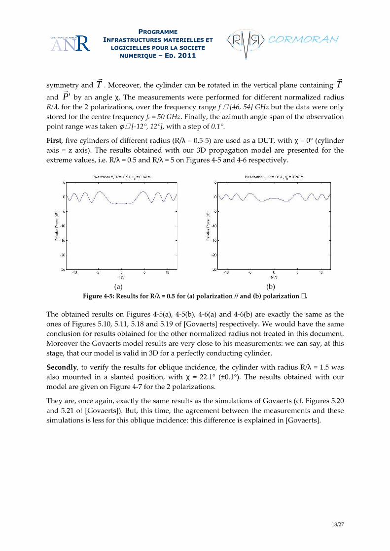
First, five cylinders of different radius (R/λ = 0.5-5) are used as a DUT, with χ = 0° (cylinder
axis = z axis). The results obtained with our 3D propagation model are presented for the
extreme values, i.e. R/λ = 0.5 and R/λ = 5 on Figures 4-5 and 4-6 respectively.
(a)
(b)
Figure 4-5: Results for R/λ = 0.5 for (a) polarization // and (b) polarization ⊥.
The obtained results on Figures 4-5(a), 4-5(b), 4-6(a) and 4-6(b) are exactly the same as the
ones of Figures 5.10, 5.11, 5.18 and 5.19 of [Govaerts] respectively. We would have the same
conclusion for results obtained for the other normalized radius not treated in this document.
Moreover the Govaerts model results are very close to his measurements: we can say, at this
stage, that our model is valid in 3D for a perfectly conducting cylinder.
Secondly, to verify the results for oblique incidence, the cylinder with radius R/λ = 1.5 was
also mounted in a slanted position, with χ = 22.1° (±0.1°). The results obtained with our
model are given on Figure 4-7 for the 2 polarizations.
They are, once again, exactly the same results as the simulations of Govaerts (cf. Figures 5.20
and 5.21 of [Govaerts]). But, this time, the agreement between the measurements and these
simulations is less for this oblique incidence: this difference is explained in [Govaerts].
Page 19
PROGRAMME
INFRASTRUCTURES MATERIELLES ET
LOGICIELLES POUR LA SOCIETE
NUMERIQUE – ED. 2011
19/27
(a)
(b)
Figure 4-6: Results for R/λ = 5 for (a) polarization // and (b) polarization ⊥.
(a) (b)
Figure 4-7: Results for χ = 22.1° and R/λ = 1.5 for (a) polarization // and (b) polarization ⊥.
5. COMPARISON WITH UR1 SERIES S2 MEASUREMENT CAMPAIGN
Finally, we have compared the developed model described in this report with measurements
made by UR1 team in the Satimo SG32 near-field antenna measurement chamber of IETR.
The measurement campaign description is detailed in Part 2 of [Mhedhbi 1]. The chamber
and the measurement platform (with an antenna and the considered cylinder called
phantom) are described in details in [Mhedhbi 1]. Moreover, the Receiver Point is considered
to be far from the cylinder.
5.1. PHANTOM CHARACTERISTICS
The custom built phantom was a nearly cylindrical plastic bottle filled with MLS1800
phantom liquid. The size of the phantom (height = 140 mm and R = 35 mm (cf. Figure 2-9 of
[Mhedhbi 1] )) was chosen to represent a human arm, while still being light enough for the
platform to support it. The complex permittivity of the phantom liquid was given in
[Mhedhbi 2] for the frequency range [300 MHz, 3 GHz] and summarized in Table 5-1.
Interpolation of the dielectric characteristics of the phantom liquid is possible in frequency
Page 20
PROGRAMME
INFRASTRUCTURES MATERIELLES ET
LOGICIELLES POUR LA SOCIETE
NUMERIQUE – ED. 2011
20/27
range of Table 5-1 but the measurements were made in the [800 MHz, 5.95 GHz] frequency
range. So we don’t have access to the dielectric properties of the cylinder between 3 GHz and
5.95 GHz: we decided to use, for this frequency range, the dielectric properties given by
[Koutitas] based on the “Muscle” model: 2.48' == rr εε and mS /7.4=σ , values used,
in this article, for a frequency of 5 GHz.
f (GHz) 0.3 0.6 0.9 1.2 1.5 1.8 2.1 2.4 2.7 3 'rε 58.15 57.03 55.99 54.94 53.64 52.63 51.67 50.40 49.28 47.82
"rε 20.28 13.96 12.90 13.44 14.14 14.86 15.72 16.73 17.53 18.31
σ (S/m) 0.34 0.47 0.65 0.90 1.22 1.49 1.84 2.23 2.63 3.06
Table 5-1: Dielectric parameters of the phantom liquid
given in the [300 MHz, 3GHz] frequency range
5.2. UTD MODEL ADAPTATION
The only measurement series of [Mhedhbi 1] that is interesting for the present developed
propagation model is the series S2: this series was done to measure how the antenna
response varies in the presence of the phantom with various antenna-phantom distances (we
will call “d” this antenna-phantom distance). The measurements were made for 0° ≤ φ < 360°
and 0° < θ < 180° with a step of approximately 2°. Antenna Th1 was used for all runs of Series
S2. Data file ‘S2R1’ gives us the antenna response. Data files ‘S2R2’ to ‘S2R23’ gives us the
measurement with phantom at different radial distances using the groove, from d= 30 mm
(File ‘S2R2’) to d = 135 mm (File ‘S2R23’), with a distance step of 5 mm.
Moreover, we could use the antenna response of ‘S2R1’ file in our model in order to take into
account the real antenna used for measurements. Indeed, the antenna Th1 is not exactly
isotropic in polarization θ (corresponding to the polarization ⊥ used before) and has less
gain in polarization φ (corresponding to the polarization // used before) than in polarization
θ. This last remark makes us finding the exact directions (φe, θe) of the emitted rays in
direction of the considered interaction (reflection or attachment point). For the moment, only
a comparison in 2D between our model results and the measurements is done so we have
only θ = 90°. So we make a simple linear interpolation between 2 measurements points of
S2R1 to find the exact value of antenna response in the direction of the considered ray.
Therefore, the incident field at the interaction point PI, which is at a distance sI from Tx, will
finally be expressed as:
( ) ( )I
jks
eeI
i
s
eFPE
I−
⊥ ⋅= θφ ,//, (24)
with the couple ( ) ( ) ( ) ( )iii
R
I
I sQorsQsQsP 2311 ,,,,, = according to the studied ray, and
( )eeF θφ , will be the antenna response in the direction (φe, θe) of the studied incident field.
Page 21
PROGRAMME
INFRASTRUCTURES MATERIELLES ET
LOGICIELLES POUR LA SOCIETE
NUMERIQUE – ED. 2011
21/27
5.3. 2D COMPARISON
Comparisons between UTD results and measurement are only given for a 2D configuration,
i.e. in the azimuth plane (θ = 90° and 0°< φ< 360°) because we have to adapt the model
(bilinear interpolation of the antenna response has not been performed for the moment) for a
comparison in 3D. We decided to present in this report the comparisons made for 3 different
distances d between the antenna and the cylinder: 3 cm, 9 cm and 13 cm. The results are
given and analyzed below for these 3 different distances, for 3 frequencies:
• f=900 MHz : the lowest frequency for which we know the exact dielectric properties
of the cylinder;
• f=3 GHz : the highest frequency for which we know the exact dielectric properties of
the cylinder;
• f=5.95 GHz : the highest frequency for which we have measurements results and for
which we use the cylinder dielectric properties of [Koutitas].
5.3.1 FOR A DISTANCE OF 3 CM
Figure 5-1 gives the obtained results for the UTD developed model and the measurements
for 900 MHz. The comparison is not convincing for polarization θ (cf. Figure 5-1(a)), i.e. the
maxima and the minima for the model and the measurements seems to be in “phase
opposition”. It is not the case in polarization φ (cf. Figure 5-1(b)), apart from the case of φ =
180° for which the model predicts a maximum and the measurements a minimum. For 900
MHz, the wavelength is λ = 33.33 cm which is large enough regarding the distance and the
cylinder radius: we are maybe at the limit of UTD theory application, which explains that the
results are not good for this first distance.
(a)
(b) Figure 5-1: Comparison between UTD results and measurements for f = 900 MHz
for (a) polarization θ and (b) polarization φ
On the other hand, for 3 GHz and 5.95 GHz (cf. Figures 5-2 and 5-3 respectively), results are
very good in polarization θ (cf. Figures 5-2(a) and 5-3(a) respectively): the model predicts a
maximum at φ = 180°, which was expected from the theory because the “creeping waves”
Page 22
PROGRAMME
INFRASTRUCTURES MATERIELLES ET
LOGICIELLES POUR LA SOCIETE
NUMERIQUE – ED. 2011
22/27
called rays 1 and 2 above, arrived in phase at the receiver in a 2D configuration. The
measurements give also a maximum for this particular value of θ, weaker than for the model
at 3 GHz but greater than for the model at 5.95 GHz. This predicted field in the shadow zone
is the first improvement regarding the 3D additive model of [Mhedhbi 1] which doesn’t
predict anything in the shadow zone although, as it is highlighted by the UR1
measurements, a diffracted field exists and presents a maximum at φ = 180° for 2D
configuration.
Concerning the polarization φ, comparison is quite good for 3 GHz (cf. Figure 5-2(b)): more
oscillations are observed for the UTD results but the “shape” of the 2 curves are globally the
same. But we notice a “phase opposition” in the case of 5.95 GHz (cf. Figure 5-3(b)): maybe
other propagation phenomena have to be taken into account (diffractions by the top and the
bottom of the cylinder could have more influence in the phase of the received field because
the wavelength is weaker than the ones corresponding to 900 MHz and 3 GHz).
(a)
(b) Figure 5-2: Comparison between UTD results and measurements for f = 3 GHz
for (a) polarization θ and (b) polarization φ
(a)
(b) Figure 5-3: Comparison between UTD results and measurements for f = 5.95 GHz
for (a) polarization θ and (b) polarization φ
Page 23
PROGRAMME
INFRASTRUCTURES MATERIELLES ET
LOGICIELLES POUR LA SOCIETE
NUMERIQUE – ED. 2011
23/27
5.3.2 FOR A DISTANCE OF 9 CM
Figure 5-4 gives the results for 900 MHz: the comparison between model and measurements,
regarding the case of d = 3 cm studied previously, is quite good. The maximum at φ = 180°,
for polarization θ in the shadow zone (cf. Figure 5-4(a)), is obtained for the measurements as
well as for the UTD model: maybe it is due to the fact that, this time, the distance d is larger.
Concerning polarization φ (cf. Figure 5-4(b)), results are quite good but with the same
conclusion as for d = 3 cm: for φ = 180°, the model predicts a maximum and the
measurements a minimum.
(a)
(b) Figure 5-4: Comparison between UTD results and measurements for f = 900MHz
for (a) polarization θ and (b) polarization φ
Figures 5-5 and 5-6 give the comparison results for 3 GHz and 5.95 GHz respectively. We
notice, for these 2 frequencies and polarization θ (cf. Figures 5-5(a) and 5-6(a) respectively for
3 GHz and 5.95 GHz), a very good correspondence between the model predicted results and
the measurements, with the same conclusions as for the case of d = 3 cm.
(a)
(b) Figure 5-5: Comparison between UTD results and measurements for f = 3 GHz
for (a) polarization θ and (b) polarization φ
Page 24
PROGRAMME
INFRASTRUCTURES MATERIELLES ET
LOGICIELLES POUR LA SOCIETE
NUMERIQUE – ED. 2011
24/27
For polarization φ and 3 GHz (cf. Figure 5-5(b)), more oscillations are observed for the UTD
results but the curves “shape”, as it was already the case for 900 MHz, are nearly the same.
For polarization φ and 5.95 GHz (cf. Figure 5-6(b)), comparison is better than for d = 3 cm,
with little more oscillations in the case of the measurements, maybe due to the diffracted
fields at the top and bottom of the cylinder.
(a)
(b) Figure 5-6: Comparison between UTD results and measurements for f = 5.95 GHz
for (a) polarization θ and (b) polarization φ
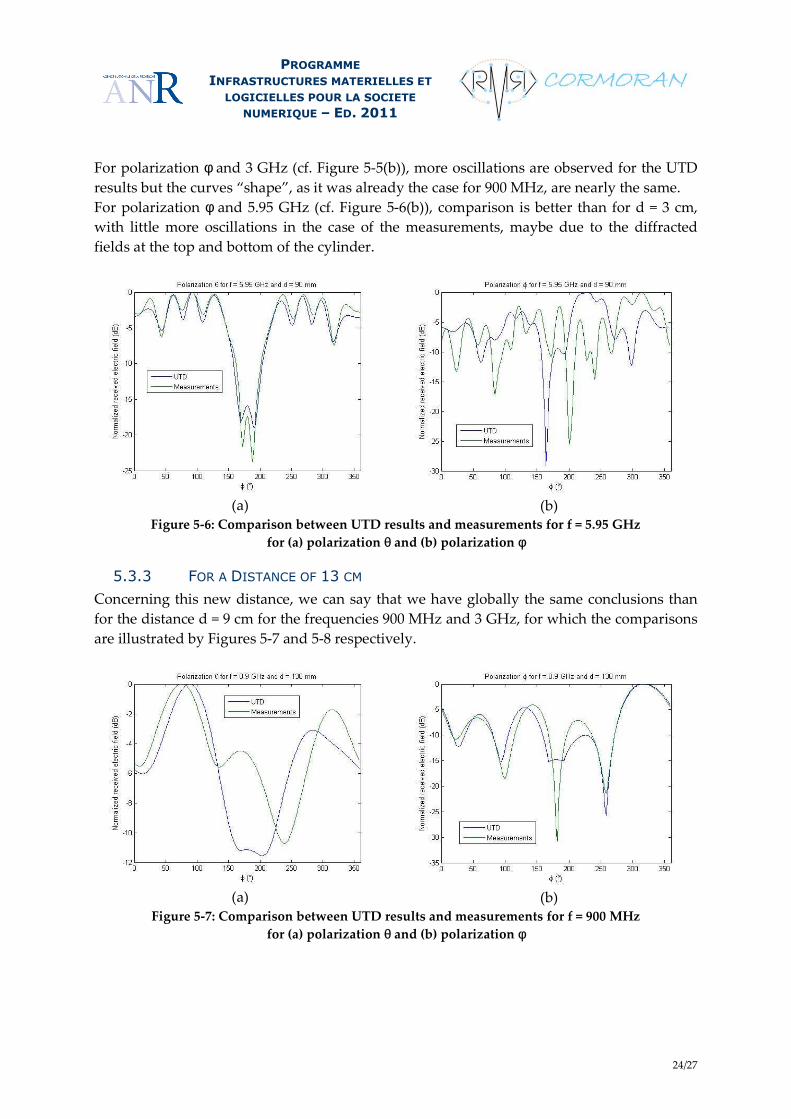
5.3.3 FOR A DISTANCE OF 13 CM
Concerning this new distance, we can say that we have globally the same conclusions than
for the distance d = 9 cm for the frequencies 900 MHz and 3 GHz, for which the comparisons
are illustrated by Figures 5-7 and 5-8 respectively.
(a)
(b) Figure 5-7: Comparison between UTD results and measurements for f = 900 MHz
for (a) polarization θ and (b) polarization φ
Page 25
PROGRAMME
INFRASTRUCTURES MATERIELLES ET
LOGICIELLES POUR LA SOCIETE
NUMERIQUE – ED. 2011
25/27
(a)
(b) Figure 5-8: Comparison between UTD results and measurements for f = 3 GHz
for (a) polarization θ and (b) polarization φ
On the other hand, new conclusions appear for the comparison in the case of 5.95 GHz, as
illustrated by Figure 5-9.
For polarization θ (cf. Figure 5-9(a)), the comparison between the model and the
measurement results in the shadow region (168°< φ< 192°) is quite good. The problem
appears in the lit region in which we notice 1 more oscillation in the case of the UTD model:
but globally, the results “shapes” are quite the same.
For polarization φ (cf. Figure 5-9(b)), UTD model varies a little more rapidly than the
measurements, which was the inverse case for 2 distances studied previously. But, globally,
the obtained curves for the UTD model and the measurements have the same shape.
(a)
(b) Figure 5-9: Comparison between UTD results and measurements for f = 5.95 GHz
for (a) polarization θ and (b) polarization φ
Page 26
PROGRAMME
INFRASTRUCTURES MATERIELLES ET
LOGICIELLES POUR LA SOCIETE
NUMERIQUE – ED. 2011
26/27
6. CONCLUSIONS
A 3D deterministic propagation model, based on the ray-tracing technique and the UTD,
developed for the particular case of a 3D single dielectric cylinder of finite length, has been
described and validated in 2D (for conducting and dielectric cylinders) and 3D (conducting
cylinder). Moreover, the first 2D comparisons of the model with the UR1 measurements
series S2 presented in [Mhedhbi 1] are quite encouraging. 3D comparisons with these same
measurements will follow: for this, we have to modify the 3D UTD received electric field
computed with our model (a bilinear interpolation has to be applied on the 3D antenna
response in order to use the good value of antenna gain in the direction of the considered
emitted ray). Moreover, if these new comparisons reveal a good correspondence between
UTD model results and measurements, this new UTD model will be validated in 3D for a
dielectric cylinder, which is not available in the literature for the moment (cf. Part 4 of this
report).
Then, we could model 2 other possible scenarios concerning the transmitter and the receiver
point positions towards the cylinder: the “Radiation” scenario (when the Transmitter (the
Receiver) is on the cylinder and the Receiver (the Transmitter) is far from the cylinder) and
the “Coupling” scenario (when both Transmitter and Receiver are on the cylinder). These
scenarios imply the computation of new integrals, different from the Pekeris function
expressed in equation (19). We can think also to develop the model for not only a circular
cylinder but for the more general case of an elliptic cylinder.
Then we can study the possibility of adapting the present described model for the scenario of
several cylinders in order to really model the human body. After, we can imagine a dynamic
model taking into account the human body motion... Then we could imagine a scenario with
several persons.
The originality of the model developed in this report is its deterministic nature and its ability
to take into account the dielectric nature of the human body. Fast statistical models already
exist but don’t model the electromagnetic wave paths. Other techniques (as FDTD (“Finite
Difference Time Domain”)) model the propagation environment in a very detailed way but
with a very long computation time. The UTD model is an intermediate model in terms of
propagation environment description and computation time. If it could be optimized in term
of computation time and, if it could be adapted for a complete human body (i.e. several
cylinders), it maybe could be used as a future WBAN model...
7. REFERENCES
[Mhedhbi 1] M. Mhedhbi, Stéphane Avrillon, Bernard Uguen, Melsuine Pigeon, Raffaele
D’Errico and Pierre Pasquero“, D2.1 - On-Body Antennas Characterization & Exploitable
Radiation Properties”, Technical Report, CORMORAN (ANR 11-INFR-010) Project , 57
pages, October 31, 2012.
[McNamara] D.A. McNamara, C.W.I. Pistorius, J.A.G. Malherbe “Introduction to the
Uniform Geometrical Theory of Diffraction”, Artech House, Boston, 1990.
Page 27
PROGRAMME
INFRASTRUCTURES MATERIELLES ET
LOGICIELLES POUR LA SOCIETE
NUMERIQUE – ED. 2011
27/27
[Pathak] P.H. Pathak, W.D. Burnside and R.J. Marhefka, “A Uniform GTD Analysis of the
Diffraction of Electromagnetic Waves by a Smooth Convex Surface”, IEEE Trans. on
Antennas and Propagation, Vol. AP-28, N°5, pp. 631-642, September 1980.
[Hussar] P.E. Hussar, “A Uniform GTD Treatment of Surface Diffraction by Impedance and
Coated Cylinders“, IEEE Trans. on Antennas and Propagation, Vol. 46, N°7, pp. 998-1008,
July 1998.
[Govaerts] H.J.F.G. Govaerts, “Electromagnetic Wave Scattering by a Circular Cylinder of
Arbitrary Radius”, Report of Graduation Work, performed October 1992 – August 1993, 62
pages.
[Glaeser] G. Glaeser, “Reflections on Spheres and Cylinders of Revolution“, Journal for
Geometry and Graphics, Vol. 3, N°2, pp. 121-139, 1999.
[Kouyoumjian] R.G. Kouyoumjian and P.H. Pathak, “A Uniform Geometrical Theory of
Diffraction for an Edge in Perfectly Conducting Surface”, Proceedings of the IEEE, Vol. 62,
N°11, pp. 1148-1461, November 1974.
[Plouhinec] E. Plouhinec, “Etude et Extension de Modèles de Prédiction de la Propagation.
Elaboration d’un Serveur Expert Multi-Modèles”, PhD Dissertation D 00-13, INSA de
Rennes, Décembre 2000.
[Bouche] D. Bouche and F. Molinet, “Méthodes Asymptotiques en Electromagnétisme”,
Springer, 416 pages, 1994.
[Abramovitz] M. Abramovitz and I.A. Stegun, “Handbook of Mathematical Functions”,
Dover Publications Inc., New-York, 1965.
[Wait] J.R. Wait and A.M. Conda, “Diffraction of Electromagnetic Waves by Smooth
Obstacles for Grazing Angles”, Journal of Research of the National Bureau of Standards, Vol.
63D, N°2, pp. 181-197, September-October 1959.
[Pearson] L. Wilson Pearson, “A Scheme for Automatic Computation of Fock-Type Integrals”,
IEEE Trans. on Antennas and Propagation, Vol. 35, N° 10, pp. 1111-1118, October 1987.
[Medgyesi] L.N. Medgyesi-Mitschang, D-S. Wang, “Hybrid Solutions for Large-Impedance
Coated Bodies of Revolution”, IEEE Trans. on Antennas and Propagation, Vol. AP-34, N°11,
pp. 1319-1328, November 1986.
[Mhedhbi 2] M. Mhedhbi, “Requirements for UWB Antenna Electromagnetic Simulations”,
CORMORAN Working Document, October 23, 2012.
[Koutitas] G. Koutitas, “Multiple Human Effects in Body Area Networks“, IEEE Antennas
and Wireless Propagation Letters, Vol. 9, pp. 938-941, 2010.


![SEVENTH FRAMEWORK PROGRAMME Research Infrastructures · Annual Report [4]) to include a summer internship programme called the PRACE Summer of HPC (SoHPC) and coordinated PRACE Campus](https://static.documents.pub/doc/80x56/5fce6a29f3cc127dad5482a8/seventh-framework-programme-research-infrastructures-annual-report-4-to-include.jpg)


