Programming Language Interfaces for Time-Varying Multivariate Visualization

Jian Huang (presented by Wesley Kendall)The University of Tennessee, Knoxville

SciDAC Institute of Ultrascale Visualization

Multivariate Temporal Features in Scientific Data

IEEE Visualization Tutorial 2009

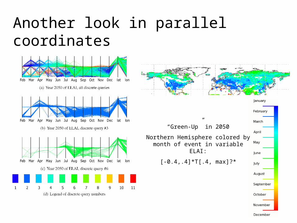
What is a feature?

What can you show me?

• A critical gap:– What do you want to see?– Show me what ever you find then.

• Too many variables to look at side by side• Too many time steps to examine one by

one• Too many models/run – to

compare/contrast

What can you show me?

• A critical gap:– Often scientists know what they want to see– But cannot provide a formal quantitative

description

Extreme Complexity Ultrascale• Scientific visualization faces problems

more complex than ever before by orders of magnitude – Complexity: carbon, biogeochemical, evolution, coupling– Number of variables: >100– Temporal resolution + span: every 3 min, 1000 years

(1.75e8)– Spatial resolution: 22km 1km– Size of ensemble runs : 50 1000

• Qualitative user concepts:– When does the growing season start?

• Domain specific programming language methods

– Specify events in an expressive, concise and powerful way

• Any persistent trends of event changes– Has the beginning of the growing season shifted in time

in recent decades? How are different locations affected?

User Concepts

Concept-Driven Visualization• As visual summaries, the benefits are:

– Data reduction– Semantic meaning– Focus– Easily multivariate and temporal– Iteratively refined and recorded

1. Define neighborhood2. Establish relevant data ranges3. Draw up clauses

Relational Patterns in Local Distribution

Spatial Neighborhood Query

With typical 1D transfer function Neighborhood Query

freq(nonbackground) > freq(background)

Temporal Neighborhood Query

Positive and negative covariance between two

timesteps

Fuzzy Matching

We want to show locations that:– match to a degree (score opacity)– match a subset of inequalities (combination

color)

Evaluating a Query

• For each location– For each clause– If TRUE

score = 1 tag bit set

– Otherwise score = f(distance)

< 1

Visualizing a Query

• All locations scored and the rendered• Sum of clause scores opacity• Clause bitfield color

– Bitfield indexes into colormap on the GPU– 2|clauses| possible bitfield configurations

mean temperature and precipitation between decades 2000-2009 and 2090-2099

Specifying Temporal features

• User concepts about temporal events are often “story” like

• Uncertainty expressed via regular expression

• *.mp3, %sale%, img[0-3][0-9].png

• Modeled after regex, but need to answers where and when an event occurs

TimeMarks

For example: [-.4,.4]*T[.4, max]?*– For each location, find time step T sandwiched

between zero or more changes in [-.4, .4] and at least one change of more than .4

• T – TimeMark: when event occurs• Automatic expansion into substantiated

queries• Combine primitives in time sequence

Meta-Queries Meta-Queries

“Green-Up”: Northern Hemisphere colored by month of event in variable ELAI.

[-.4,.4]*T[.4, max]?*

2050

2051

2052

“First Snow”: Northern Hemisphere colored by month of event in variable FSNO

???[min, 0.7]*T[0.7, max]?*

2050

2051

2052

Meta-Queries Meta-Queries

Another look in parallel coordinates

“Green-Up” in 2050

Northern Hemisphere colored by month of event in variable ELAI:

[-0.4,.4]*T[.4, max]?*

Complexity of Meta Queries

• Many cases could lead to exponential problem spaces

• Fortunately, the data access patterns are not random (except in rare cases)

Concept-Driven Visualization• Required infrastructural support:

– Parallelism– Scalable data structures– Optimal use of parallel I/O

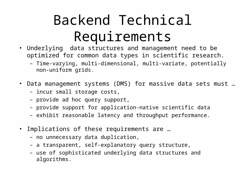
Backend Technical Requirements

• Underlying data structures and management need to be optimized for common data types in scientific research.– Time-varying, multi-dimensional, multi-variate, potentially non-

uniform grids.

• Data management systems (DMS) for massive data sets must …– incur small storage costs,– provide ad hoc query support,– provide support for application-native scientific data– exhibit reasonable latency and throughput performance.

• Implications of these requirements are …– no unnecessary data duplication,– a transparent, self-explanatory query structure,– use of sophisticated underlying data structures and algorithms.

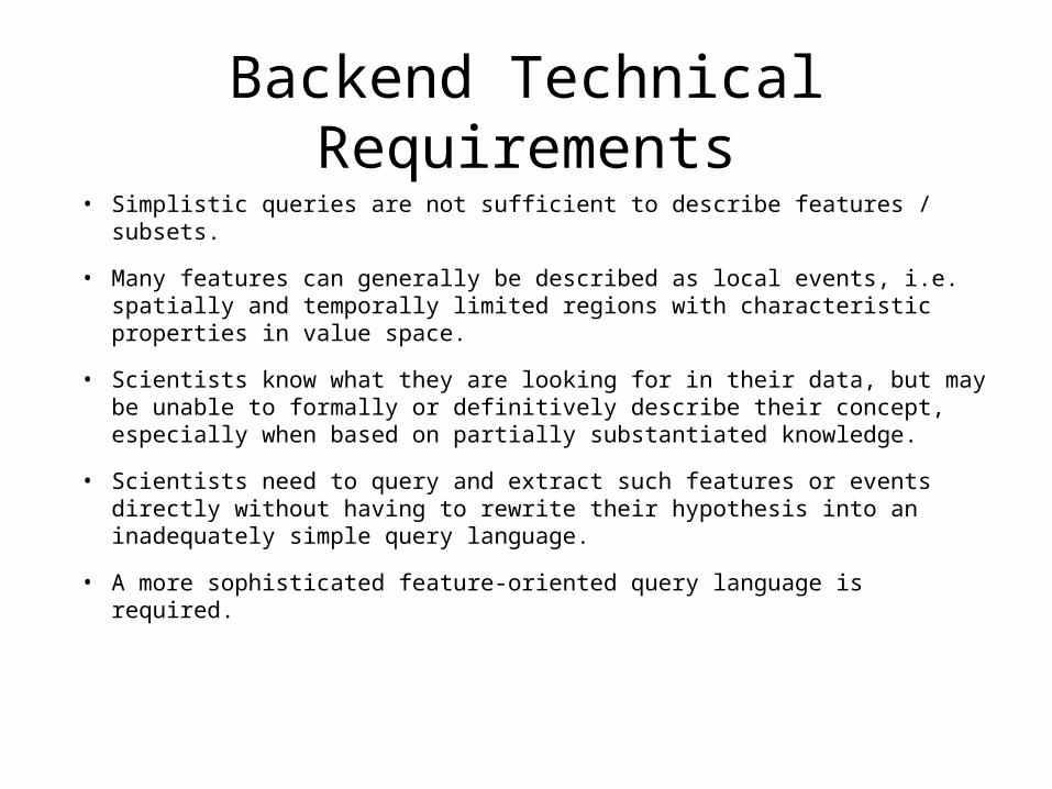
Backend Technical Requirements

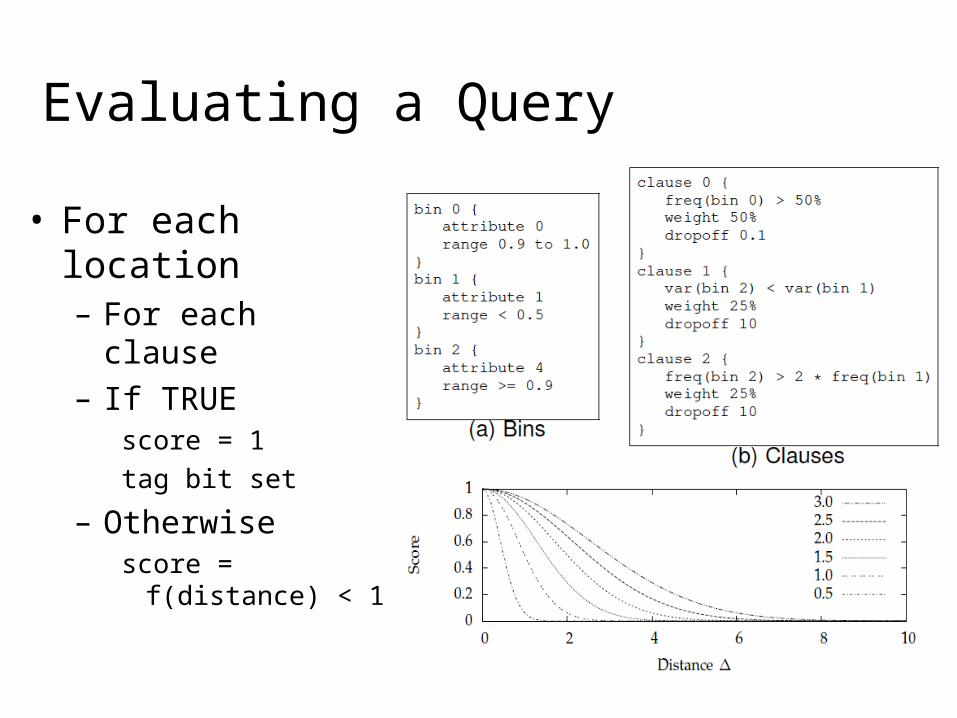
• Simplistic queries are not sufficient to describe features / subsets.

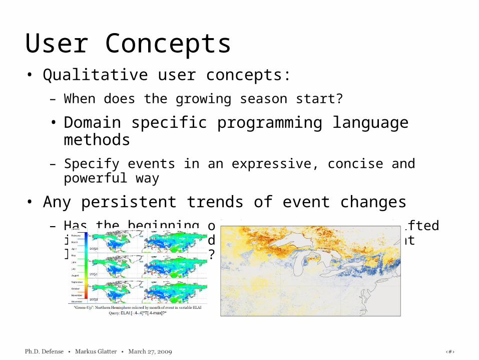
• Many features can generally be described as local events, i.e. spatially and temporally limited regions with characteristic properties in value space.

• Scientists know what they are looking for in their data, but may be unable to formally or definitively describe their concept, especially when based on partially substantiated knowledge.

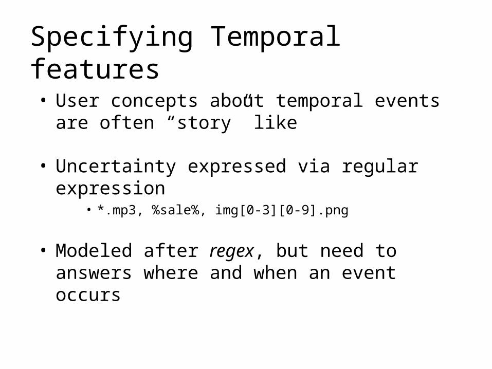
• Scientists need to query and extract such features or events directly without having to rewrite their hypothesis into an inadequately simple query language.

• A more sophisticated feature-oriented query language is required.

Related Work• Large data management in visualization

– Data partitioning (blocks, “bricks”)– Efficient searching using tree-based data structures:

• Interval tree, k-d tree quad-tree, octree, etc.• Bitmap indexing

– Relational Database Management Systems (RDBMS)

• (Programming) languages in visualization:– More versatile and flexible compared to GUIs.– Alter GPU shader programs on the fly: “Scout”– VTK provides Tcl/Tk and Python bindings.

• Large data sets need to be partitioned for data distribution and load-balancing.

• Break up data set into data items containing– spatial and temporal location (x,y,z,t),– a value for each data variable.

e.g. {x=1; y=2; z=3; t=10; density=2.7; entropy=.7}

• Implications– Yields increase in total data size!– Number of data items can be enormous!– But: Load-balancing can be applied on the level of data

items.

Data Organization

• Load-balancing by breaking up locality within the dataset.• Optimized data access by using a B-tree like structure to

skip irrelevant data items on top of a linear search.• Discard unwanted data items upon distribution (data

items are independent of any structural meta-information)• Compress blocks of data items to trade memory space

vs. access time, decompress on access.

Query-Driven Visualization

Voxel Data

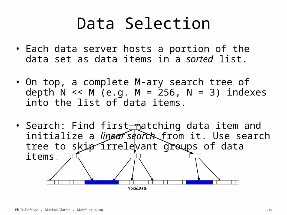
• Each data server hosts a portion of the data set as data items in a sorted list.

• On top, a complete M-ary search tree of depth N << M (e.g. M = 256, N = 3) indexes into the list of data items.

• Search: Find first matching data item and initialize a linear search from it. Use search tree to skip irrelevant groups of data items.

Data Selection

Voxel Data

• Observation: Data items are independent of any structural meta-information (e.g. a grid).– Unwanted data items can be deleted before distribution

to data servers.– This counterbalances the increase of data set size.

• Compress the linear list of data items.– Trade-off: memory space vs. access time– Blocks of data items are decompressed on the fly.– Since linear list is sorted, high compression rates (20:1)

are possible in many cases.

Enhancements

Scalability Tests: the data

• NASA's Moderate Resolution Imaging Spectro-radiometer (MODIS) database, continuously updated

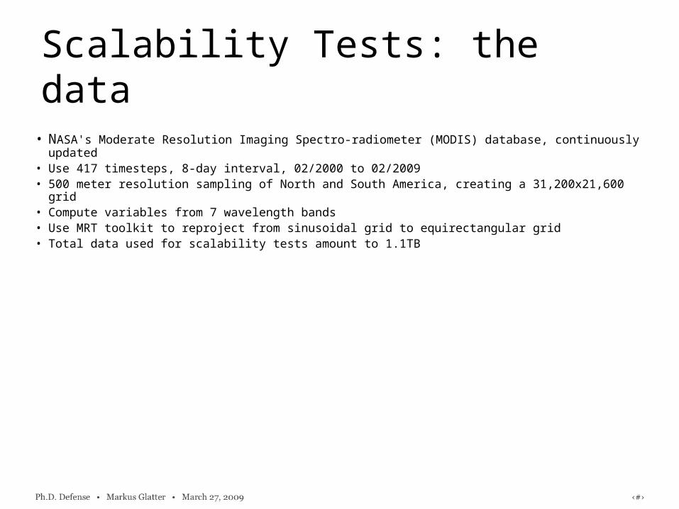
• Use 417 timesteps, 8-day interval, 02/2000 to 02/2009• 500 meter resolution sampling of North and South America, creating a 31,200x21,600 grid• Compute variables from 7 wavelength bands• Use MRT toolkit to reproject from sinusoidal grid to equirectangular grid• Total data used for scalability tests amount to 1.1TB

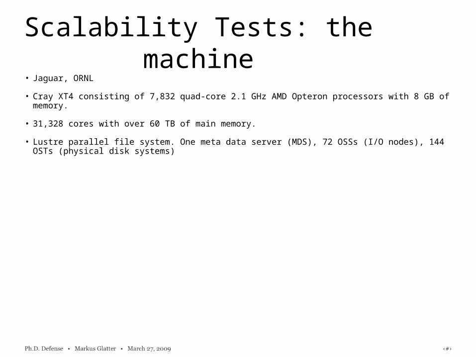
Scalability Tests: the machine

• Jaguar, ORNL

• Cray XT4 consisting of 7,832 quad-core 2.1 GHz AMD Opteron processors with 8 GB of memory.

• 31,328 cores with over 60 TB of main memory.

• Lustre parallel file system. One meta data server (MDS), 72 OSSs (I/O nodes), 144 OSTs (physical disk systems)

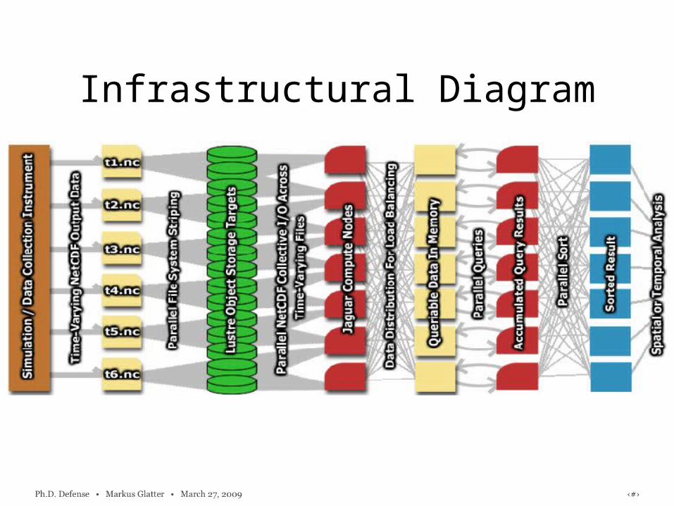
Infrastructural Diagram

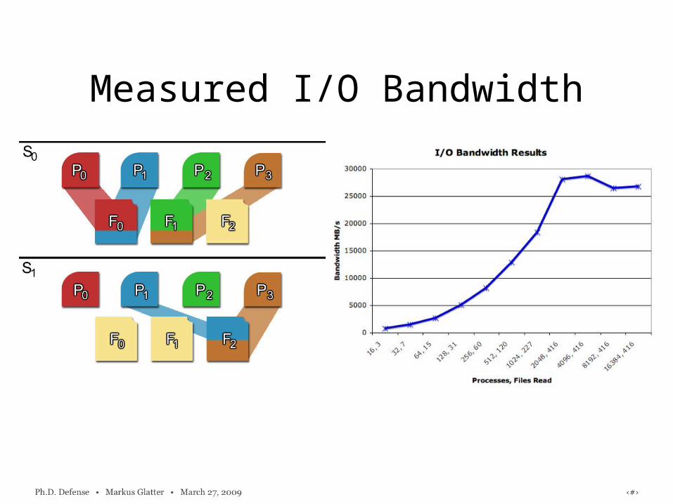
Measured I/O Bandwidth

Distribution and Query Overheads

Climate Science - Drought Assessment

• NDVI and NDWI can be good indicators of drought, and NDDI (Normalized Difference Drought Index) can be computed by

NDDI = (NDVI - NDWI) / (NDVI + NDWI)

• We use a similar method of drought assessment by querying for: NDVI < 0.5 and NDWI < 0.3

• After queries are issued, result is sorted in spatial order

• Temporal overlap can then be computed– look for 0.5 < NDDI < 1 for at least 4 timesteps (1 month) in a row

• We also placed one more restriction and throw out the areas where the event happened more than one time, finding only the areas where abnormal drought conditions occur

Drought Assessment

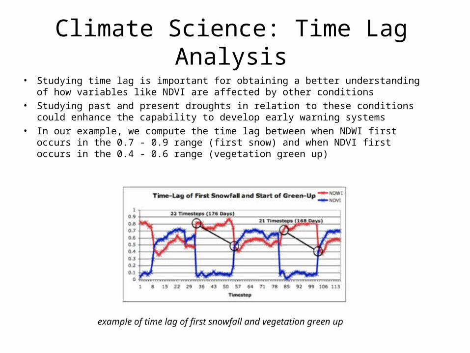
Climate Science: Time Lag Analysis

• Studying time lag is important for obtaining a better understanding of how variables like NDVI are affected by other conditions

• Studying past and present droughts in relation to these conditions could enhance the capability to develop early warning systems

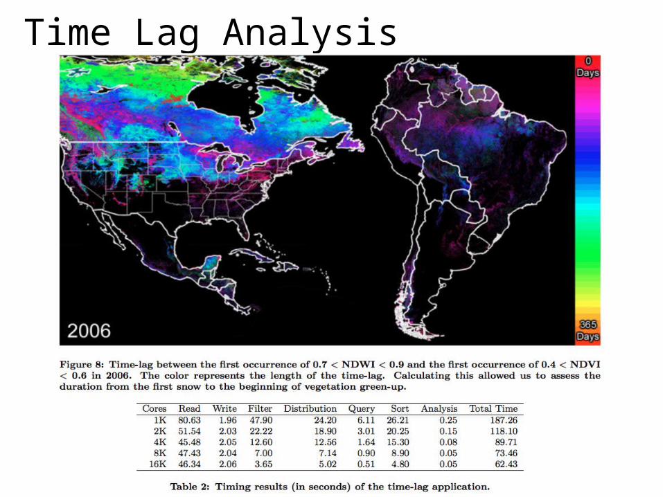
• In our example, we compute the time lag between when NDWI first occurs in the 0.7 - 0.9 range (first snow) and when NDVI first occurs in the 0.4 - 0.6 range (vegetation green up)

example of time lag of first snowfall and vegetation green up

Time Lag Analysis

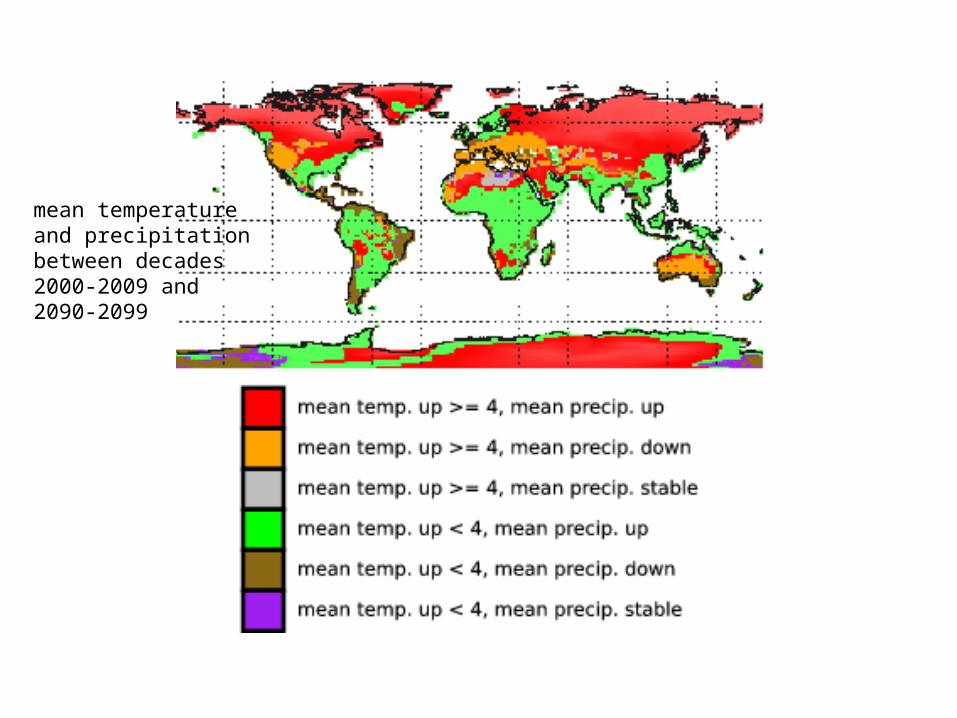
Conclusion• Creating single images as summarizing visualization of

a high-level event to study climate change

• Feature specification that empowers “eye-balling” should be studied in depth, in addition to feature extraction and rendering

• Programming language type of methods have offered encouraging results

• It is crucial to have truly scalable parallel infrastructure for visualizing terascale data and beyond

References• Wesley Kendall, Markus Glatter, Jian Huang, Tom Peterka, Robert

Latham and Robert Ross, Terascale Data Organization for Discovering Multivariate Climatic Trends, SC'09, November 2009, Portland, OR.

• C. Ryan Johnson and Jian Huang, Distribution Driven Visualization of Volume Data, IEEE Transactions on Visualization and Computer Graphics, 15(5):734-746, 2009.

• Markus Glatter, Jian Huang, Sean Ahern, Jamison Daniel, and Aidong Lu, Visualizing Temporal Patterns in Large Multivariate Data using Textual Pattern Matching, IEEE Transactions on Visualization and Computer Graphics, 14(6):1467-1474, 2008.

• Markus Glatter, Colin Mollenhour, Jian Huang, and Jinzhu Gao, Scalable Data Servers for Large Multivariate Volume Visualization, IEEE Transactions on Visualization and Computer Graphics, 12(5):1291-1299, 2006.

Acknowledgements• Current Students:

– Wesley Kendall• Graduated students:

– Dr. Markus Glatter, Dr. C. Ryan Johnson, Dr. Rob Sisneros, Dr. Josh New

– Brandon Langley, Colin Mollenhour• Collaborators DOE SciDAC Ultravis Institute (www.ultravis.org)

– Rob Ross, Tom Peterka, Kwan-Liu Ma, Han-Wei Shen, Ken Moreland, John Owens

• Collaborators at Oak Ridge National Laborartory– Sean Ahern, Forrest Hoffman, David Erickson.

• Our funding were provided by DOE SciDAC, DOE Early Career PI Award, NSF ACI and CNS programs.