Properties of a Cutting Plane Method for SemidefiniteProgramming1

Kartik Krishnan Sivaramakrishnan

Axioma, Inc.Atlanta, GA 30350kksivara@gmail.com

http://www4.ncsu.edu/˜kksivara

John E. Mitchell

Mathematical SciencesRensselaer Polytechnic Institute

Troy, NY 12180mitchj@rpi.edu

http://www.rpi.edu/˜mitchj

Last Revised July 11, 2012 (submitted for publication).

Abstract

We analyze the properties of an interior point cutting plane algorithm that is basedon a semi-infinite linear formulation of the dual semidefinite program. The cutting planealgorithm approximately solves a linear relaxation of the dual semidefinite program inevery iteration and relies on a separation oracle that returns linear cutting planes. Weshow that the complexity of a variant of the interior point cutting plane algorithm isslightly smaller than that of a direct interior point solver for semidefinite programswhere the number of constraints is approximately equal to the dimension of the matrix.Our primary focus in this paper is the design of good separation oracles that returncutting planes that support the feasible region of the dual semidefinite program. Theintersection of a cutting plane at a boundary point y with the tangent cone at that pointgives a face of the tangent cone; we propose to use the dimension of this face to measurethe strength of the cutting plane, we characterize the supporting hyperplanes that givehigher dimensional faces of the tangent cone, and show how such cutting planes can befound efficiently. Our procedures are analogous to finding facets of an integer polytope incutting plane methods for integer programming. We illustrate these concepts with twoexamples in the paper. We present computational results that highlight the strength ofthese cutting planes in a practical setting. Our technique of finding higher dimensionalcutting planes can conceivably be used to improve the convergence of the spectral bundlemethod of Helmberg et al. [10, 11], and the non-polyhedral cutting surface algorithmsof Sivaramakrishnan et al. [38] and Oskoorouchi et al. [27, 28].

Keywords: Semidefinite programming, interior point methods, regularized cuttingplane algorithms, maximum eigenvalue function, cone of tangents.

1The second author is supported in part by NSF grant numbers DMS–0317323 and DMS–0715446.

1 Introduction

A semidefinite programming problem requires minimizing a linear objective function in sym-metric matrix variables subject to linear equality constraints together with a convex con-straint that these variables be positive semidefinite. The tremendous activity in semidefiniteprogramming was spurred by the discovery of efficient interior point algorithms for solvingsemidefinite programs, and important applications of semidefinite programming in combina-torial optimization, control, robust optimization, and polynomial optimization (see Laurentand Rendl [19], for example).

Primal-dual interior point methods (IPMs) (see the surveys by de Klerk [7] and Monteiro[23]) are currently the most popular techniques for solving semidefinite programs. However,current semidefinite solvers based on IPMs can only handle problems with dimension n andnumber of equality constraints k up to a few thousands (see, for example, Toh et al. [40]).Each iteration of a primal-dual IPM solver needs to form a dense Schur matrix, store thismatrix in memory, and finally factorize and solve a dense system of linear equations of sizek with this coefficient matrix. Several techniques have been developed to solve large scaleSDPs; these include: the low rank factorization approach of Burer and Monteiro [6]; thespectral bundle methods of Helmberg et al. [10, 11]) and Nayakkankuppam [24]; parallelimplementations of primal-dual IPMs on shared memory (see Borchers and Young [5]) anddistributed memory (see Yamashita et al. [42]) systems; and interior point cutting planealgorithms (see Sivaramakrishnan et al. [37, 38], Oskoorouchi et al. [27, 28], and Sherali andFraticelli [36]).

In this paper, we investigate the properties of the interior point cutting algorithms pre-sented in Krishnan et al. [15, 16, 38]. The methods are based on a semi-infinite linearformulation of a semidefinite program and they use an interior point cutting frameworkto approximately solve the underlying semidefinite program to 2-3 digits of accuracy. Re-cently Qualizza et al. [33] have employed a variant of this algorithm to solve semidefiniterelaxations of quadratically constrained quadratic problems. We introduce the semi-infiniteformulation in section 2 and give a brief description of the algorithm in section 3. The algo-rithm uses a primal-dual interior point method to approximately solve the linear relaxationsthat arise at each iteration of the cutting plane algorithm. Theoretically, it is possible to usea volumetric interior point method to solve the relaxations. We show in section 4 that thecomplexity of a volumetric interior point cutting plane algorithm for solving a semidefiniteprogram to a prescribed tolerance ε > 0 is slightly less than that of a primal-dual IPM, atleast for a semidefinite program where the number of constraints is approximately equal tothe dimension of the matrix.

Our interior cutting plane algorithm solves a linear relaxation of the dual semidefiniteprogram. In every iteration, the algorithm calls a separation oracle that adds cutting planesto strengthen the current relaxation. The convergence of the cutting plane algorithm can

1

be improved by adding strong cutting planes; this is the focus of section 5. We show that wecan always find a hyperplane that supports the feasible region of the semidefinite program.In cutting plane methods for integer programming (see Nemhauser and Wolsey [25]), thestrongest cutting planes are facet inequalities that describe the higher dimensional facesof the integer polytope. Each supporting hyperplane induces a face of the tangent cone.The dimension of this face is one measure of the strength of this hyperplane. When theprimal semidefinite program has k constraints and the nullity of the dual slack matrix atthe support point is 1, we show that the dimension of the face of the tangent cone definedby the hyperplane is k − 1. Further, if the nullity of the active dual slack matrix is r, wedescribe how to generate a cutting plane that gives a face of the tangent cone of dimensionat least k − r. We illustrate these concepts with two representative examples in section 6,and some computational results can be found in section 7.Notation: The set of n×n symmetric matrices is denoted Sn. The set of positive semidef-inite n× n matrices is denoted Sn+. The requirement that a matrix be positive semidefiniteis written X � 0. Matrices are represented using upper case letters and vectors using lowercase letters. Given an n-vector v, the diagonal n × n matrix with the ith diagonal entryequal to vi for i = 1, . . . , n is denoted Diag(v). The n × n identity matrix is denoted In;when the dimension is clear from the context, we omit the subscript. The Frobenius innerproduct of two m × n matrices A and B is denoted A • B; if the matrices are symmetricthis is equal to the trace of their product, denoted trace(AB).

2 Semi-infinite formulations for semidefinite programming

Consider the semidefinite programming problem

min C •Xs.t. A(X) = b (SDP)

X � 0

with dualmax bT y

s.t. AT y + S = C (SDD)S � 0

where X,S ∈ Sn+, C ∈ Sn, b and y are vectors in IRk, and A is a linear function mappingSn to IRk. We can regard A as being composed of k linear functions, each representedby a matrix Ai ∈ Sn, so the constraint A(X) = b is equivalent to the k linear constraintsAi •X = bi, i = 1, . . . , k. The expression AT y is equivalent to

∑ki=1 yiAi.

We make the following two assumptions.

Assumption 1 The matrices Ai, i = 1, . . . , k are linearly independent in Sn.

2

Assumption 2 There exists a constant a ≥ 0 such that every X satisfying AX = b alsosatisfies trace(X) = a.

Helmberg [9] shows that every semidefinite program whose primal feasible set is boundedcan be rewritten to satisfy Assumption 2. The following lemma is a consequence of thisassumption.

Lemma 1 [9] There exists a unique vector y satisfying AT y = I, the identity matrix.

Consider any feasible point y in (SDD). The point (y− µy) is strictly feasible in (SDD)for µ > 0. Indeed, the dual slack matrix at this new point is S = (C − AT (y − µy)) =(C −AT y + µI) � 0. So, Assumption 2 ensures that (SDD) has a strictly feasible (Slater)point. This assumption ensures that we have strong duality at optimality, i.e. the optimalobjective values of (SDP) and (SDD) are equal. Moreover, the primal problem (SDP)attains its optimal solution.

Note that the convex constraint X � 0 is equivalent to

ηTXη = ηηT •X ≥ 0 ∀η ∈ B (1)

where B is a compact set, typically {η : ||η||2 ≤ 1} or {η : ||η||∞ ≤ 1}. These constraintsare linear inequalities in the matrix variable X, but there is an infinite number of them.Thus, a semidefinite program is a semi-infinite linear program in IR

n(n+1)2 variables.

We now consider two semi-infinite linear programs (PSIP)

min C •Xs.t. A(X) = b (PSIP)

ηTXη ≥ 0, ∀η ∈ B

max bT y

s.t. AT y + S = C (DSIP)ηTSη ≥ 0, ∀η ∈ B

for (SDP) and (SDD), respectively. Note that X is n × n and symmetric, so (PSIP) has(n+12

)= n(n+1)

2 = O(n2) variables. In contrast, there are k variables in (DSIP). We havek ≤

(n+12

)(from Assumption 1). Therefore, it is more efficient to deal with (DSIP), since

we are dealing with smaller linear programs (but see also the discussion at the end of thissection).

We discuss the finite linear programs (LDR) and (LPR) and some of their propertiesbelow. Given a finite set of nonzero vectors {ηi, i = 1, . . . ,m}, we obtain the followingrelaxation

max bT y

s.t.k∑j=1

yj(ηTi Ajηi) ≤ ηTi Cηi, i = 1, . . . ,m (LDR)

3

of (SDD). The dual to (LDR) can be expressed as follows:

min C •(

m∑i=1

xiηiηTi

)

s.t. A(

m∑i=1

xiηiηTi

)= b (LPR)

xi ≥ 0, i = 1, . . . ,m.

The convex constraint S � 0 is also equivalent to

P TSP � 0, ∀P ∈ IRn×r, r < n, and P TP = Ir. (2)

This allows one to develop a semi-infinite semidefinite formulation for (SDD) where thesemidefinite cone of size n in (SDD) is replaced with an infinite number of semidefinitecones of size r < n. An overview of various techniques to update relaxations involvingfinite subsets of these cones in interior cutting plane algorithms can be found in Krishnanand Mitchell [17]. In particular, in Krishnan and Mitchell [16] the relaxations are linearprograms; in Sivaramakrishnan et al. [38] and Oskoorouchi and Goffin [27], the relaxationsare conic programs over a linear cone and several semidefinite cones of small size; and in thespectral bundle algorithm of Helmberg and Rendl [11], the relaxations are conic programsover one linear cone and one semidefinite cone.

Theorem 1 Let y∗ and x∗ be optimal solutions to (LDR) and (LPR), respectively.

1. The matrix X∗ =m∑i=1

x∗i ηiηTi is feasible in (SDP).

2. Let S∗ = (C −AT y∗). We have X∗ • S∗ = 0. Furthermore, if S∗ � 0 then X∗S∗ = 0,and X∗ is an optimal solution to (SDP).

Proof: The primal conic program (LPR) is a constrained version of (SDP). Therefore,

any feasible solution x∗ in (LDR) gives a X =m∑i=1

x∗i ηiηTi that is feasible in (SDP). We have

X∗ • S∗ =m∑i=1

x∗i ηiηTi • (C −AT y∗)

=m∑i=1

x∗i ηTi (C −AT y∗)ηi

= 0

from the complementary slackness at optimality for (LPR) and (LDR). If S∗ = (C−AT y∗)is positive semidefinite, then it is feasible in (SDD). Moreover, X∗ � 0, S∗ � 0, andX∗ • S∗ = 0 together imply X∗S∗ = 0 (see Alizadeh et al. [1]).

The following theorem is due to Pataki [30] (also see Alizadeh et al. [1]):

4

Theorem 2 There exists an optimal solution X∗ with rank r satisfying the inequalityr(r+1)

2 ≤ k, where k is the number of constraints in (SDP ).

The theorem suggests that an upper bound on the rank of an optimal solution X∗ isr∗ = b

√2kc, where k is the number of equality constraints in (SDP). Suppose S∗ is the dual

slack matrix at an optimal solution y∗ to (SDD). The complementary slackness conditionsX∗S∗ = 0 at optimality imply that X∗ and S∗ share a common eigenspace. Moreover,the positive eigenspace of X∗ corresponds to the nullspace of S∗ (see Alizadeh et al. [1]).Therefore, Theorem 2 also provides an upper bound on the dimension of the nullspace ofS∗.

Let q =n(n+ 1)

2− k. It is possible to use a nullspace representation to reformulate

(SDP) as a semi-infinite programming problem with q variables. This is advantageous if qis smaller than k, in particular if q is O(n). Let B : Sn → IRq be the nullspace operatorcorresponding to A, so the range of BT is exactly the kernel of A. From Assumption 1,we can regard B as being composed of q linear functions, each represented by a matrixBi ∈ Sn, and these matrices are linearly independent in Sn. Let X0 be a feasible solutionto the linear equality constraints A(X) = b. The set of feasible solutions to A(X) = b isthe set of all matrices of the form X = X0 − BT (u) for some u ∈ IRq. The problem (SDP)can then be written equivalently as

minu,X

C •X0 − C • BT (u)

s.t. BT (u) +X = X0 (SDPN)X � 0.

The problem (SDPN) is in exactly the form of (SDD), so we can construct a linear program-ming relaxation of it in the form (LDR), with q variables. We return to this alternativerepresentation when discussing the complexity of the algorithm in section 4. (A similarnullspace representation of linear programming problems has been analyzed in the interiorpoint literature; see, for example, Todd and Ye [39] and Zhang et al. [43].)

3 Cutting plane algorithms for semidefinite programming

Let

Y = {y ∈ IRk : S = (C −AT y) � 0}= {y ∈ IRk : λmax(AT y − C) ≤ 0}

(3)

be the convex set containing the feasible solutions to (SDD). The goal of cutting planemethods that solve (SDD) is to find an optimal point that maximizes bT y over Y . Thereare three important ingredients in this algorithm:

1. The technique used to update the relaxations (LPR) and (LDR) in every iteration.

5

2. The choice of the query point y.

3. Given a query point y, a separation oracle that either (a) tells us that y ∈ Y inwhich case we try to improve the objective function bT y, or (b) returns a separatinghyperplane that separates y from the set Y .

Choosing an optimal solution y to (LDR) as the next query point is a bad idea (see Example1.1.2 on page 277 of Hiriart-Urruty and Lemarechal [13]). Instead, one adopts strategieswhere the idea is to choose a more central point y in the feasible region of (LDR) as thenext query point. These strategies include using a quadratic penalty term as in a bundlemethod (see Helmberg and Rendl [11]), using an analytic center with objective functioncuts used to push the iterates towards an optimal solution (see Oskoorouchi and Goffin[27], for example), and only solving (LDR) approximately with an interior point method(see Sivaramakrishnan et al. [38], for example).

The main contribution of this paper is to design an efficient separation oracle that canbe utilized within a cutting plane algorithm for solving (SDD). We discuss the choice ofgood cutting planes in section 5 and illustrate these choices with examples in section 6.

We first introduce several separating hyperplanes for the feasible set Y . The maximumeigenvalue function λmax(AT y − C) is a convex non-smooth function, with a discontinuousgradient whenever this eigenvalue has a multiplicity greater than one. The subdifferentialto λmax(AT y − C) at y = y (see Hiriart-Urruty and Lemarechal [13]) is given by

∂λmax(AT y − C) = conv{A(ppT ) : pT (AT y − C)p = λmax(AT y − C), pT p = 1} (4)

where conv denotes the convex hull operation. There is also an alternate description

∂λmax(AT y − C) = {A(PV P T ) : trace(V ) = 1, V � 0} (5)

where P ∈ IRn×r is an orthonormal matrix containing the eigenspace of λmax(AT y − C)(see Overton [29]). We note that (5) does not involve the convex hull operation. We willuse the second expression (5) in Theorem 5 to derive an expression for the normal cone forthe maximum eigenvalue function. Any subgradient from (4) gives the valid inequality

λmax(AT y − C) ≥ λmax(AT y − C) +A(ppT )T (y − y) ∀y. (6)

Now given the query point y, we first check for feasibility, i.e. λmax(AT y − C) ≤ 0. If y isnot feasible, then we can construct a cut

λmax(AT y − C) +A(ppT )T (y − y) ≤ 0 (7)

To motivate this consider (7) with the reversed inequality. This would imply λmax(AT y −C) > 0 from (6), and so y also violates the convex constraint. It follows that any feasible y

6

satisfies (7). Using the fact that p is a normalized eigenvector corresponding to λmax(AT y−C), we can rewrite (7) as

pT (C −AT y)p ≥ 0 (8)

which is a valid cutting plane which is satisfied by all the feasible y. From linear algebra(see Horn and Johnson [14]), we have

λmax(AT y − C) = max {ηT (AT y − C)η : ||η||2 = 1}. (9)

Moreover, any eigenvector η corresponding to a positive eigenvalue of the matrix (AT y−C)gives a valid cutting plane ηT (C − AT y)η ≥ 0. However, these cutting planes are weakerthan the cutting plane (8) that corresponds to the most positive eigenvalue of (AT y − C).Cutting planes can also be found using the ∞-norm; for details, see Krishnan and Mitchell[18].

Algorithm 1 presents the overall interior point cutting plane algorithm for solvingsemidefinite programs. For the implementation details of a more sophisticated algorithmsimilar to Algorithm 1 see Sivaramakrishnan et al. [38]. Procedures to warm-start the newrelaxations with strictly feasible starting points are discussed in Sivaramakrishnan et al.[38]. These are extensions of techniques given in Mitchell and Todd [22]. The relaxationsare only solved approximately in Step 3 because the iterates are then more centered, whichleads to stronger cutting planes and improved warm starting. We show later in theorem 4that the vector y = ym − λy constructed in Step 6 is on the boundary of Y and provides alower bound. The algorithm can be refined to drop unimportant constraints; for details seeSivaramakrishnan et al. [38]. We illustrate two iterations of the cutting plane algorithm infigure 1.

Computational results with Algorithm 1 can be found in Sivaramakrishnan et al. [38].Moreover, computational results obtained with the related spectral bundle and ACCPMalgorithms can be found in Helmberg et al. [10, 11] and Oskoorouchi et al. [27, 28], respec-tively.

7

Algorithm 1 (Interior point cutting plane algorithm)

1. Initialize: Set m = 1. Choose an initial LP relaxation (LDR) that has a boundedoptimal solution. Let xm and ym be feasible solutions in (LPR) and (LDR),respectively. Choose a tolerance parameter β > 0 and a termination parameterε > 0.

2. Warm start the current relaxation: Generate strictly feasible starting pointsfor (LPR) and (LDR).

3. Solve the current relaxation: Solve the current relaxations (LPR) and (LDR)with the strictly feasible starting points from Step 3 to a tolerance β. Let xm andym be the current solutions to (LPR) and (LDR), respectively. Update the upperbound using the objective value to (LPR).

4. Separation Oracle: Call the separation oracle at the point ym. If the oraclereturns a cutting plane, update (LPR) and (LDR).

5. Optimality check: If the oracle reported feasibility in Step 4 then reduce β bya constant factor. Else, β is unchanged. If β < ε, we have an optimal solution,STOP.

6. Update lower bound: If the oracle reported feasibility in Step 4 then bT ym

provides the current lower bound on the optimal objective value. Else, Sm =(C − AT ym) is not psd. Perturb Sm (using the vector y from Lemma 2) togenerate y, that is on the boundary of Y and whose objective value bT y providesa lower bound. Update the lower bound.

7. Loop: Set m = m+ 1 and return to Step 2.

4 Complexity of the interior point cutting plane algorithm

It must be mentioned that a semidefinite program was known to be solvable in polynomialtime, much before the advent of interior point methods. In fact we can use the polynomialtime oracle for a semidefinite program mentioned in section 3 in conjunction with theellipsoid algorithm to solve this problem in a polynomial number of arithmetic operations.It is interesting to compare the worst case complexity of such a method, with that of interiorpoint methods.

The ellipsoid algorithm (for example, see Grotschel et al. [8]) can solve a convex pro-gramming problem of size k with a separation oracle to an accuracy of ε, in O(k2 log(1

ε ))

8

FEASIBLE REGIONOF DUAL LP RELAXATION

y(m−1)

y(m+1)

ystart(m)

DUALSDP

REGIONIN

y SPACE

y(m) ystart(m+1)

ycheck(m)

ycheck(m+1)

Figure 1: Solving the SDP via a cutting plane algorithm: In the (m − 1)th iteration,the point y(m − 1) is outside the feasible region of (SDD). The oracle returns the uniquehyperplane that supports the dual SDP feasible region at ycheck(m) and cuts off y(m−1). Astrictly feasible restart point ystart(m) is found. The new LP relaxation is approximatelysolved using an interior point method, giving y(m), that is inside the feasible region of(SDD). In this case, we tighten the tolerance to which the LP relaxation is solved, while thefeasible region of the relaxation is unchanged. The LP is solved with starting point y(m),giving y(m + 1) that is outside the feasible region of (SDD). The oracle returns a cuttingplane that supports the dual feasible region at ycheck(m + 1). Note that the boundary of(SDD) has a kink at ycheck(m + 1), and there are several supporting hyperplanes at thispoint. The separation oracle returns the tightest hyperplane at ycheck(m + 1) that cutsoff y(m + 1). Note that this hyperplane corresponds to a higher dimensional face of SDPfeasible region.

9

calls to this oracle, assuming the solution exists in a ball of radius O(1ε ) centered at the

origin. The number of arithmetic operations is O(k2 log(1ε )T + k4 log(1

ε )), where T is thenumber of operations required for one call to the oracle. Each iteration of the ellipsoidalgorithm requires O(k2) arithmetic operations, which accounts for the k4 log(1

ε ) term inthe complexity measure.

The interior point cutting plane algorithm with the best complexity is a volumetricbarrier method, due to Vaidya [41] and refined by Anstreicher [2] and Ramaswamy andMitchell [34]. The volumetric center minimizes the determinant of the Hessian of thestandard potential function −

∑i ln si, where s is the vector of dual slacks in the linear

programming relaxation. This is closely related to finding the point where the volume ofthe inscribing Dikin ellipsoid is largest. (See Mitchell [21] for a survey of interior pointpolynomial time cutting plane algorithms.) This algorithm requires O(k log(1

ε )) iterations,with each iteration requiring one call to the oracle and O(k3) other arithmetic operations.Thus, the overall complexity is O(k log(1

ε )T + k4 log(1ε )) arithmetic operations. Note that

the number of calls to the oracle required by the volumetric algorithm is smaller than thecorresponding number for the ellipsoid algorithm. This complexity of O(k log(1

ε )) calls tothe separation oracle is optimal — see Nemirovskii and Yudin [26].

The oracle for semidefinite programming requires the determination of an eigenvectorcorresponding to the smallest eigenvalue of the current dual slack matrix. Let us examinethe arithmetic complexity of this oracle. Let us assume that our current iterate is y ∈ IRk.

1. We first have to compute the dual slack matrix S = (C −k∑i=1

yiAi), where C, S, and

Ai, i = 1, . . . , k are in Sn. This can be done in O(kn2) arithmetic operations.

2. We then compute λmin(S), and an associated eigenvector η. This can be done inO(n3) arithmetic operations using the QR algorithm for computing eigenvalues, andpossibly in O(n2) operations using the Lanczos scheme, whenever S is sparse.

3. If λmin(S) ≥ 0, we are feasible, and therefore we cut based on the objective function.This involves computing the gradient of the linear function, and this can be done inO(k) time.

4. On the other hand if λmin(S) < 0, then we are still outside the SDP cone; we can now

add the valid constraintk∑i=1

yi(ηTAiη) ≤ ηTCη, which cuts off the current infeasible

iterate y. The coefficients of this constraint can be computed in O(kn2) arithmeticoperations.

It follows that the entire oracle can be implemented in T = O(n3 + kn2) time.We summarize this discussion in the following theorem.

10

Theorem 3 A volumetric cutting plane algorithm for a semidefinite programming problemof size n with k constraints requires O((kn3 + k2n2 + k4) log(1

ε )) arithmetic operations. Anellipsoid algorithm cutting plane method requires O((k2n3 + k3n2 + k4) log(1

ε )) arithmeticoperations.

Let us compare this with a direct interior point approach. Interior point methods (seeMonteiro [23] for more details) can solve an SDP of size n, to a precision ε, in O(

√n log(1

ε ))iterations (this analysis is for a short step algorithm). As regards the complexity of aniteration:

1. We need O(kn3 + k2n2) arithmetic operations to form the Schur matrix M . This canbe brought down to O(kn2 + k2n) if the constraint matrices Ai are rank one as in thesemidefinite relaxation of the maxcut problem (see Laurent and Rendl [19]).

2. We need O(k3) arithmetic operations to factorize the Schur matrix, and compute thesearch direction. Again, this number can be brought down if we employ iterativemethods.

The overall scheme can thus be carried out in O(k(n3 + kn2 + k2)√n log(1

ε )) arithmeticoperations. (We may be able to use some partial updating strategies to factorize M andimprove on this complexity.) Thus, if k = O(n) then the complexity of the volumetriccutting plane algorithm is slightly smaller than that of the direct primal-dual interior pointmethod. Thus we could in theory improve the complexity of solving an SDP using a cuttingplane approach.

Note also that if q =n(n+ 1)

2− k is O(n), we can use the nullspace representation

(SPDN) to improve the complexity estimate given in theorem 3. In particular, the problem(SDPN) is in exactly the form of (SDD), so the cutting plane approach of section 3 canbe applied to it directly. It follows from theorem 3 that (SDP) can be solved in O((qn3 +q2n2 + q4) log(1

ε )) arithmetic operations using a volumetric barrier cutting plane algorithm.This is again superior to the complexity derived above for a direct interior point methodfor solving (SDP) if q = O(n).

5 Properties and generation of good cutting planes

The practical convergence properties of the interior point cutting plane algorithm could bestrengthened by developing a better separation oracle. In this section, we investigate thevalid inequalities returned by the separation oracle in the cutting plane algorithm. Givena point y /∈ Y , the cutting plane algorithm with the 2-norm oracle generates constraintsof the form ηT (AT y)η ≤ ηTCη, where η is an eigenvector of the current dual slack matrixS = (C − AT y) with a negative eigenvalue. These constraints separate y from Y . Wefocus on the most negative eigenvalue. We show that the constraint corresponding to any

11

eigenvector coming from the most negative eigenvalue is tight in Theorem 4. When theminimum eigenvalue has multiplicity one, we show that this constraint defines a facet ofthe tangent cone in Theorem 7. Furthermore, we construct a method for deciding betweeneigenvectors when the multiplicity is greater than one in section 5.3, culminating in thestrong lower bound on the dimension of a cutting plane in Theorem 9.

We show first that there is a point y on the boundary of Y that satisfies the cuttingplane constraint at equality. Let η be an eigenvector of S of norm one corresponding to themost negative eigenvalue of S, and let λ denote this eigenvalue. Define

y = y − λy (10)

where y is the vector in Lemma 1. The dual slack matrix at y is S = S + λI, which ispositive semidefinite, so y ∈ Y . Further, η is in the nullspace of S.

Theorem 4 Let η be an eigenvector of the current dual slack matrix S with minimumeigenvalue. The constraint ηT (C−AT y)η ≥ 0 is satisfied at equality by the feasible point y.

Proof: We have S = C − AT y and η is in the nullspace of this matrix. Thus we haveηTSη = 0 and so this feasible y ∈ Y satisfies the new constraint at equality.

We let r denote the nullity of S. Let S have the eigendecomposition

S = [Q1 Q2]

[Λ 00 0

] [Q1

T

Q2T

], (11)

where Q = [Q1 Q2] is an orthonormal matrix and Λ is a (n− r)× (n− r) positive diagonalmatrix. This eigendecomposition is used to characterize the cone of tangents at y in section5.1. Further analysis of the cases where r = 1 and r > 1 can be found in sections 5.2 and5.3, respectively.

5.1 Cone of tangents and the normal cone

A valid linear inequality for a convex set gives a face of the convex set, namely the in-tersection of the set with the hyperplane defined by the inequality. For a full-dimensionalpolyhedron, the only inequalities that are necessary are those describing the facets of thepolyhedron (see Nemhauser and Wolsey [25]). A more general convex set may not have anyfacets; for example, all the nontrivial faces of the unit ball in IRk have dimension 0. In orderto gauge the strength of a supporting hyperplane, we propose looking at the face of thetangent cone given by its intersection with the supporting hyperplane. For a polyhedron,this gives the face of the polyhedron defined by the supporting hyperplane; for the unit ballin IRk, the intersection of the (unique) supporting hyperplane at a boundary point x withthe tangent cone at x has dimension k − 1. We formalize the idea of a face of the tangentcone in the following definition.

12

Definition 1 Let Y be a nonempty closed convex set in IRk. For any point y ∈ IRk, thedistance from y to Y is defined as the distance from y to the unique closest point in Y andis denoted dist(y, Y ). Let y be a point on the boundary of Y . The cone of feasible directions,the tangent cone, and the normal cone at y are defined as

dir(y, Y ) = {d : y + td ∈ Y for some t > 0}

tcone(y, Y ) = cl(dir(y, Y )) (closure of dir(y, Y ))

= {d : dist(y + td, Y ) = O(t2)}

ncone(y, Y ) = {v : dT v ≤ 0, ∀d ∈ tcone(y, Y )}.

Given a supporting hyperplane H for Y , the face of the tangent cone defined by H at y is

tcf(y, Y,H) = {d ∈ tcone(y, Y ) : y + d ∈ H}.

A convex subset F of Y is a face of Y if

x ∈ F , y, z ∈ Y , x ∈ (y, z) implies y, z ∈ F ,

where (y, z) denotes the line segment joining y and z. Note that {u : u = y + d, d ∈tcf(y, Y,H)} contains the face H ∩ Y of Y .

The equivalence of the two definitions of tcone follows from page 135 of Hiriart-Urruty andLemarechal [12]. The geometry of semidefinite programming is surveyed by Pataki [31].Conceptually, the idea of a face of the tangent cone will be used as an analogue of the ideaof a face of a polyhedron. In sections 5.2 and 5.3, we show that if Y is full-dimensional andif the inequality arises from an eigenvector of S with smallest eigenvalue then the dimensionof the face of the tangent cone is related to the dimension of the corresponding eigenspace.We will illustrate these concepts with the following example:

Example 1 Consider

Y =

y ∈ IR2 : S =

y1 y2 0y2 y1 − 3 00 0 y1 − 4

� 0

.Consider the point y = [3 2]T and let S = (C − AT y). We have λ = λmin(S) = −1with multiplicity 2 and so y 6∈ Y . One can easily verify that y = [1 0]T . The pointy = (y − λy) = [4 2]T ∈ Y . This example is illustrated in figure 2. We have

tcone(y, Y ) = {d ∈ IR2 : 5d1 − 4d2 ≥ 0, d1 ≥ 0} andncone(y, Y ) = {v ∈ IR2 : 4v1 + 5v2 ≤ 0, v2 ≥ 0}.

The extreme rays of ncone(y, Y ) are [−1 0] and [−5 4], respectively. The first ray gives thelinear constraint y1 ≥ 4 which gives the face of the tangent cone generated by d1. The second

13

�������������

Convex set Y

vy������ d2

�d1

Cone of tangents tcone(y, Y )

I

i

@@

@

aaaa �

Normal conencone(y, Y )

Figure 2: The tangent cone and normal cone for Example 1

14

ray gives the linear constraint 5y1−4y2 ≥ 12 and the face of the tangent cone defined by thisconstraint at y is the halfline generated by d2. This second ray defines a face of dimension 0of the feasible region Y , but a face of dimension k− 1 of the tangent cone. It is desirable toadd constraints corresponding to higher dimensional faces of tcone(y, Y ), rather than weakerconstraints that are active at y, such as 2y1−y2 ≥ 6. The latter constraint is obtained fromthe internal ray [−2 1] in ncone(y, Y ).

In general convex programming, extreme rays of the normal cone may produce themost effective cuts, because of the duality between the normal cone and the tangent conefor convex sets [3, 35]. We characterize the normal cone for our problem and thus deriveexpressions for effective cuts; we will use these characterizations in Theorem 9 to obtain alower bound on the dimension of the face of the tangent cone defined by a hyperplane. Wewill now derive an expression for ncone(y, Y ).

Theorem 5 Assume that y satisfies λmax(AT y −C) = 0 and there exists a Slater point yssuch that λmax(AT ys − C) < 0. Then

ncone(y, Y ) = cone(∂λmax(AT y − C))= {A(Q2V Q

T2 ) : V � 0}

(12)

where cone(X) = {γx : x ∈ X, γ ≥ 0} and Q2 is the nullspace of of (AT y − C).

Proof: The proof for the first expression for ncone(y, Y ) can be found in theorem 1.3.5on page 245 of Hiriart-Urruty and Lemarechal [12]. Using the second expression (5) for thesubdifferential ∂λmax(AT y − C), we have

ncone(y, Y ) = {γA(Q2V QT2 ) : trace(V ) = 1, V � 0, γ ≥ 0}

= {A(Q2V QT2 ) : V � 0}.

In general, the cone {A(Q2V QT2 ) : V � 0} may not be closed, as in the following example

drawn from Pataki [32]:

Example 2 Take k = n = 2. Let

QT2A1Q2 =

[1 00 0

], QT2A2Q2 =

[0 11 0

].

It can be easily verified that the ray [0 1]T is not in the cone {A(Q2V QT2 ) : V � 0}, but

it is in its closure. It should be noted that the matrices A1 and A2 in this example do notsatisfy Assumption 2.

A sufficient condition (see Pataki [32]) to guarantee the closure of the cone {A(Q2V QT2 ) :

V � 0} is the existence of a y ∈ IRk such that QT2 (AT y)Q2 � 0, which is guaranteed byAssumption 2. From Lemma 1, the vector y satisfies QT2 (AT y)Q2 = I � 0.

We will now derive an expression for tcone(y, Y ).

15

Theorem 6 Assume that y satisfies λmax(AT y −C) = 0 and there exists a Slater point yssuch that λmax(AT ys − C) < 0. Then

tcone(y, Y ) = {d ∈ IRk : QT2 (ATd)Q2 � 0} (13)

where Q2 is the nullspace of (AT y − C).

Proof: We have

tcone(y, Y ) = {d ∈ IRk : dT v ≤ 0, ∀v ∈ ncone(y, Y )}= {d ∈ IRk : dT (AT (Q2V Q

T2 )) ≤ 0, ∀V � 0} (from Theorem 5)

= {d ∈ IRk : (QT2 (ATd)Q2) • V ≤ 0, ∀V � 0}= {d ∈ IRk : QT2 (ATd)Q2 � 0}.

We note that an alternative derivation for the tangent cone for the cone of positive semidef-inite matrices can be found in Bonnans and Shapiro [4].

5.2 When the nullity of the dual slack matrix equals one

If the nullity of S is equal to one, then the dimension of the face of the tangent cone isk − 1, as we show in the next theorem. This is as large as possible, of course.

Theorem 7 If the minimum eigenvalue of S has multiplicity of one with correspondingeigenvector η, then the constraint ηT (C −AT y)η ≥ 0 defines a facet of the tangent cone ofY at y.

Proof: The matrix S has an eigendecomposition

S = [Q1 η]

[Λ 00 0

] [Q1

T

ηT

](14)

where Q = [Q1 η] is an orthogonal matrix and Λ is a (n − 1) × (n − 1) positive diagonalmatrix. For any point y, define the direction d = y − y. The constraint can be writtenηT (S −ATd)η ≥ 0, or equivalently as

k∑i=1

diηTAiη ≤ 0

since η is in the nullspace of S. The supporting hyperplane H is defined by the equation

k∑i=1

diηTAiη = 0, (15)

so H = {y + d : d satisfies (15)}. Moreover from theorem 6, d ∈ tcone(y, Y ) and henced ∈ tcf(y, Y ). So, tcf(y, Y,H) has dimension k − 1.

16

�������������

Feasible region Y in y-space

for (SDD)

vyvy + εd v y + εd+ βy

ηT (C −AT y)η = 0

�A(ηηT )

Figure 3: The tangent plane defined by the cutting plane in y-space

When the multiplicity of the maximum eigenvalue is one, λmax(AT y−C) is differentiableat y = y. So, ncone(y, Y ) = A(ηηT ) (singleton set). Moreover, tcone(y, Y ) is the half space∑ki=1 diη

TAiη ≤ 0 whose boundary is the only supporting hyperplane at y = y given by(15). For an illustration of this result, see figure 3.

5.3 General values for the nullity

An upper bound on the nullity of an optimal dual slack matrix S∗ is given by Theorem 2,and this nullity is typically greater than one. In exact arithmetic, the nullity of S may beone as Algorithm 1 converges to an optimal solution to (SDD), but there are likely to beseveral very small eigenvalues. Computationally, the effective nullity of S may be greaterthan one. We will generalize Theorem 7 for the case where the nullity of S is greater thanone, to get a lower bound on the dimension of the face of the tangent cone. Let S have aneigendecomposition that is given by (11). We let r denote the nullity of S, and η denotes anyvector of norm one in the nullspace of S. We now obtain a lower bound on the dimensionof the face of the tangent cone.

Proposition 1 The dimension of the face of the tangent cone to Y at y defined by the valid

17

constraint ηT (C −AT y)η ≥ 0 is at least k −(r + 1

2

).

Proof: The columns of Q2 give a basis for the nullspace of S; denote these columns as

p1, . . . , pr. There are at least k−(r + 1

2

)linearly independent directions d satisfying the(

r + 12

)equations

pTi (ATd)pj = 0, 1 ≤ i ≤ j ≤ r. (16)

Note that η is a linear combination of the columns of Q2, so any d satisfying (16) is on thehyperplane ηT (ATd)η = 0. From Theorem 6, any direction d satisfying (16) is also in thecone of tangents to Y at y. The result follows.

In section 6, we give examples where the face of the tangent cone has dimension fargreater than that implied by Proposition 1. Eigenvectors η that make the dimension ofthe corresponding tangent plane as large as possible give the best linear approximation tothe cone of tangents. We now characterize the vectors η which will do this, leading to thestrengthened result of Theorem 9. Any element v ∈ ncone(y, Y ) gives a valid cutting planevT y ≤ vT y. The strongest constraints for tcone(y, Y ) are those where v is an extreme rayof ncone(y, Y ). We can find the extreme rays of ncone(y, Y ) by finding the extreme pointsof slices through ncone(y, Y ). We use y to define one particular slice as

Π = {v ∈ ncone(y, Y ) : yT v = 1}. (17)

We first show that Π is a closed and bounded set and that every nonzero v ∈ ncone(y, Y )can be scaled to give a point in Π.

Proposition 2 For any nonzero v ∈ ncone(y, Y ), the inner product yT v is strictly positive.Further, the set Π is compact.

Proof: Using Theorem 5, if v ∈ ncone(y, Y ) then we have v = A(Q2V QT2 ) for some

V � 0, soyT v = yTA(Q2V Q

T2 )

= (QT2 (AT y)Q2) • V= trace(V ).

Therefore,

Π = {A(Q2V QT2 ) : trace(V ) = 1, V � 0}.

We note that Π is the image under a linear transformation of the closed and bounded set{V � 0 : trace(V ) = 1}, so Π must also be closed and bounded.

18

It follows from Proposition 2 that we can find all the extreme rays of ncone(y, Y ) bysolving the semidefinite program min{gT v : v ∈ Π} for various values of g. Further, if thesolution for a particular g is unique then the optimal v is an extreme ray of ncone(y, Y ).This SDP is easy to solve, requiring just the calculation of the minimum eigenvalue of anr × r matrix.

Theorem 8 The extreme rays of ncone(y, Y ) are vectors of the form v = A(Q2uuTQT2 ),

where u is an eigenvector of minimum eigenvalue of the matrix QT2 (AT g)Q2 for some vec-tor g.

Proof: Each extreme ray is the solution to a semidefinite program of the form

min gT v

subject to A(Q2V QT2 ) − v = 0 (SP8)

yT v = 1V � 0

for some vector g. The dual of this problem is

max z

subject to QT2 (AT y)Q2 � 0yz − y = g.

Substituting y = yz − g into the first constraint and exploiting the facts that AT y = I andQT2Q2 = I, we obtain the eigenvalue problem

max z

subject to zI � QT2 (AT g)Q2. (SD8)

It follows that the optimal value z is the smallest eigenvalue of QT2 (AT g)Q2. By comple-mentary slackness, the optimal primal matrix V must be in the nullspace of the optimaldual slack matrix, giving the result stated in the theorem.

We can use the characterization of the extreme rays given in this theorem to determineexplicitly the dimension of the corresponding face of the tangent cone of Y .

Theorem 9 Let v be an extreme ray found by solving (SP8), and assume the nullity of theoptimal slack matrix in (SD8) is one. The face of the tangent cone defined by the constraintvT y ≤ vT y has dimension at least k − r.

Proof: Let u be a basis for the nullspace of the optimal slack matrix for (SD8). Fromcomplementary slackness for the (SP8) and (SD8) pair, we have v = A(Q2uu

TQT2 ), rescal-ing u if necessary. For a direction d to be on the face of the tangent cone defined by the

19

constraint, we need vTd = 0 and QT2AT (d)Q2 � 0. The equality condition can be restatedin terms of u as requiring uTQT2AT (d)Q2u = 0, or equivalently as requiring d be such thatu is in the nullspace of QT2AT (d)Q2.

Take z to be the optimal value of (SP8) and let d = yz − g. From complementaryslackness in the pair of semidefinite programs in theorem 8 we have vT d = 0. AlsoQT2AT (d)Q2 = (zI − QT2AT (g)Q2) � 0. Hence it is clear that d is in the face of thetangent cone defined by the constraint. The vector u is in the nullspace of QT2AT (d)Q2.We now exploit the hypothesis on the nullity of QT2AT (d)Q2. Without loss of generality,consider the eigendecomposition

QT2AT (d)Q2 = [U u]

[Λ 00 0

] [UT

uT

]

where Λ ≺ 0. We choose any vector of the form d = d + αd′, where d′ is chosen so that uis in the nullspace of QT2AT (d′)Q2 and α > 0 is a sufficiently small parameter determinedbelow. It is clear such a choice of d′ will guarantee that u is in the nullspace of QT2AT (d)Q2.Now

QT2AT (d)Q2 = [U u]

[Λ + αV 0

0 0

] [UT

uT

]

where V = UTQT2AT (d′)Q2U . Since Λ ≺ 0, it is clear that the matrix QT2AT (d)Q2 � 0 foran appropriate choice of α > 0.

The matrix QT2AT (d′)Q2 is r× r, so d′ ∈ IRk must satisfy r homogeneous equations foru to be in the nullspace of QT2AT (d)Q2. It follows that the dimension of the set of possibled′ is at least k − r, giving the result.

This theorem is useful in that it gives us an easy method to distinguish between differentvectors Q2u in the nullspace of the dual slack matrix S. Algorithmically, we could randomlygenerate vectors g and check whether the smallest eigenvalue of QT2AT (g)Q2 has multiplicityequal to one. If so, then we obtain a strong inequality. Note that the matrix QT2AT (g)Q2

is full rank, almost surely, since the columns of Q2 are linearly independent and sinceAssumption 2 holds. It follows that the minimum eigenvalue will have multiplicity onealmost surely.

Our idea of choosing the extreme points of the subdifferential in constructing the sepa-rating hyperplane is complementary to the notion of choosing the minimum norm subgra-dient from the subdifferential (see Chapter IX in Hiriart-Urruty and Lemarechal [13]). Thenegative of the minimum norm subgradient gives the steepest descent direction and it iscommonly employed in subgradient and bundle methods for nonsmooth optimization. The

20

problem of finding the minimum norm subgradient can be written as

min vT v

subject to v = A(Q2XQT2 )

yT v = 1X � 0.

(18)

The solution v to (18) usually occurs at an interior point of the feasible region, i.e., atan internal ray of ncone(y, Y ). Consequently, as we show in example 6.2, the generatedhyperplane defines a face of the tangent cone of low dimension.

6 Examples of the face of the tangent cone

In this section, we look at examples of faces of the tangent cone for some semidefiniteprograms. The first example in section 6.1 considers a simple second order cone constraintof size 2. Our aim is to use this example to illustrate the power of Theorem 8 in generatingstronger cutting planes. A more complicated non-polyhedral example with a large value ofr is the subject of section 6.2.

6.1 SOCP example

The second order cone constraint y21 ≥ y2

2, y1 ≥ 0, can be represented as the SDP constraint

y1

[1 00 1

]+ y2

[0 11 0

]� 0.

Consider the point y = [−1, 0]. The dual slack matrix S =

[y1 y2

y2 y1

]has a negative

eigenvalue −1 with multiplicity 2 at y. Moreover, the eigenvector corresponding to thiseigenvalue is not unique. Note that y from Lemma 1 is [1, 0]T , and y from (10) is [0, 0]T .One choice for a cutting plane would be to choose any eigenvector corresponding to theminimum eigenvalue at S. Applying the QR algorithm gives the following two choices forthe eigenvector: (1) η1 = [1, 0]T that gives the cutting plane y1 ≥ 0, and (2) η2 = [0, 1]T

that again gives the cutting plane y1 ≥ 0. Note that the face of the tangent cone definedby this constraint at this origin is the origin itself, so has dimension 0. Incidentally, theseare the eigenvectors returned by the eig routine in our implementation of the cutting planemethod in MATLAB.

The cone of tangents at the origin is

tcone = {d ∈ IR2 : d1 ≥ |d2|}

and the normal cone isncone = {d ∈ IR2 : d1 ≤ −|d2|}.

21

At the origin, we have Q2 = I. Given a vector u ∈ IR2 with ||u||22 = 1, we obtain

A(Q2uuTQT2 ) =

[−1

−2u1u2

]

and the extreme rays of the normal cone are obtained by taking u1 = ± 1√2

and u2 = ± 1√2.

By Theorem 8, we can obtain the extreme rays by first picking a vector g ∈ IR2 andthen finding an eigenvector of minimum eigenvalue of the matrix

AT g := g1

[−1 0

0 −1

]+ g2

[0 −1−1 0

]=

[−g1 −g2−g2 −g1

].

The eigenvalues of this matrix are −g1 ± g2. We have two cases:

g2 > 0: The minimum eigenvalue is −g1 − g2 and the corresponding eigenvector is u =[1, 1]T , normalized. Then

A(Q2uuTQT2 ) =

[−1−1

],

one of the extreme rays of the normal cone. This gives the cutting plane y1 + y2 ≥0. The face of the tangent cone defined by this constraint at the origin is the rayy1 + y2 = 0 that has dimension 1.

g2 < 0: The minimum eigenvalue is −g1 + g2 and the corresponding eigenvector is u =[1, −1]T , normalized. Then

A(Q2uuTQT2 ) =

[−1

1

],

the other extreme ray of the normal cone. This gives the cutting plane y1 − y2 ≥ 0.The face of the tangent cone defined by this constraint at the origin is the ray y1 = y2

that has dimension 1.

Hence, almost every choice of g leads to an extreme ray of the normal cone. The exceptionis to take g2 = 0. This returns the weaker cutting plane y1 ≥ 0, which as we discussedbefore, defines a face of the tangent cone of dimension 0.

The result of Theorem 9 may underestimate the dimension of the face of the tangentcone defined by the constraint. For this example, we have k − r = 0, and the dimension ofthe face of the tangent cone is 1.

6.2 Non-polyhedral example

TakeC = eeT − I, Ai = −eieTi , i = 1, . . . , n.

22

This is a non-polyhedral example with k = n and y = −e. We take y = e, so S = eeT andr = nullity(S) = n− 1. Thus, k − r = 1.

Any η = ei − ej with i 6= j is in the nullspace of S. The constraint becomes di + dj ≥ 0for any direction d from y. If n = 2, then r = 1 and by theorem 7 the hyperplaned1 + d2 = 0 defines a face of the tangent cone of dimension 1. In this case, we havetcone(y, Y ) = {d ∈ IR2 : d1 + d2 ≥ 0}.

Suppose, n = 3. In this case r = 2. Moreover, using MAPLE we find that

tcone(y, Y ) =

{d ∈ IR3 :

[d1 + d2 + 4d3

√3(d1 − d2)√

3(d1 − d2) 3(d1 + d2)

]� 0

},

ncone(y, Y ) =

{v ∈ IR3 :

[−3

2v3√

32 (−v1 + v2)

√3

2 (−v1 + v2) −v1 − v2 + v32

]� 0

},

and the feasible region of (SP8) is

Π =

{v ∈ IR3 : v1 + v2 + v3 = −1,

[−3

2v3√

32 (−v1 + v2)

√3

2 (−v1 + v2) −v1 − v2 + v32

]� 0

}.

Consider the hyperplane d1 + d2 = 0. The face of the tangent cone defined by this hy-perplane is the half-line {d ∈ IR3 : d1 = 0, d2 = 0, d3 ≥ 0}, that is of dimension 1.More importantly, there are no facet defining hyperplanes of dimension 2 due to the non-polyhedral nature of tcone(y, Y ). The choice of g = [1 1 0] in (SP8) gives the hyperplaned1 + d2 = 0. The minimum norm subgradient obtained from the solution to (18) gives thehyperplane d1 + d2 + d3 = 0, that intersects tcone(y, Y ) at [0 0 0] and defines a face ofthe tangent cone of dimension 0. Similarly, for n ≥ 3 every hyperplane di + dj = 0, i 6= j

defines a face of the tangent cone of dimension n− 2, since we can increase the values of dl,l 6= i, j and stay on the hyperplane as well as tcone(y, Y ). This is strictly larger than k − rfor n ≥ 4.

Now consider n = 3 and the hyperplane d1 + d2 + 4d3 = 0. The face of the tangent conedefined by this hyperplane is the halfline {d ∈ IR3 : d1 ≥ 0, d2 = d1, d3 = −2d1}, that isof dimension 1. For n = 4, we have

tcone(y, Y ) =

d ∈ IR4 :

6(d1 + d2) 2

√3(d1 − d2)

√6(d1 − d2)

2√

3(d1 − d2) 2(d1 + d2 + 4d3)√

2(d1 + d2 − 2d3)√6(d1 − d2)

√2(d1 + d2 − 2d3) (d1 + d2 + d3 + 9d4)

� 0

and the hyperplane d1 + d2 + 4d3 = 0 defines the face of the tangent cone {d ∈ IR4 : d1 =0, d2 = 0, d3 = 0, d4 ≥ 0}, that is again of dimension 1. For n ≥ 4, the hyperplanedi + dj + 4dk ≥ 0, i 6= j 6= k defines a face of the tangent cone of dimension n− 3.

Now assume n ≥ 4. We give a supporting hyperplane that defines a face of the tangentcone of dimension 0. Let η be the following vector in the nullspace of S:

ηi =

{bn2 c for i = 1, . . . , dn2 e−dn2 e for i = dn2 e+ 1, . . . , n

23

Since n ≥ 4, at least two components of η are equal to bn2 c and at least two are equal to−dn2 e. The constraint for the tangent plane becomes

∑ni=1 diη

2i = 0. For instance for n = 4,

we have η = [1 1 − 1 − 1] which gives the hyperplane d1 + d2 + d3 + d4 = 0. Moreover,this is the hyperplane returned by the minimum norm subgradient that is the solution to(18). It can be shown that this hyperplane defines a face of the tangent cone of dimension0 which is strictly smaller than k − r.

7 Computational Results

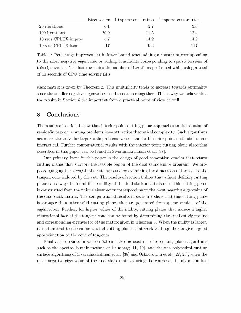
In this section, we compare the effect of adding a cutting plane corresponding to the mini-mum eigenvalue of S = (C −AT y) with adding other cutting planes. We test the approachon Ising spin glass MaxCut problems with 10000 vertices, taken from [20]. We use CPLEX12 to solve the LP relaxations on one core of an Apple Mac Pro with a 2x2.8 GHz Quad-CoreIntel Xeon processor. The most negative eigenvalue was found using the power method,applied first to find the largest eigenvalue and then applied to a shifted version of S to findthe most negative eigenvalue and a corresponding eigenvector. The tested alternative toadding this eigenvector was to sparsify it, ensuring that it still gave a violated constraint.This is a similar approach to that in [33]. We investigated adding either 10 or 20 sparseconstraints at each iteration.

In Table 1, we compare the average improvement in the lower bound on the SDP relax-ation for three instances, after 20 iterations and after 100 iterations. The initial lower boundis obtained using two sets of dual constraints: (i) the diagonal entries of S are nonnegative,and (ii) for each 2 × 2 principal minor M of S with nonzero off-diagonal, we impose theconstraint that dTMd ≥ 0, where d = (1,−1)T . For our test problems, the optimal solutionto this relaxation results in each M being positive semidefinite.

It is clear that the single eigenvector is giving better bounds than 10 or 20 sparse con-straints. The linear programs with the sparse constraints solve more quickly than the LPswith dense constraints, so we also compare the two approaches when equalizing for the timeused by CPLEX. In this comparison, the sparse approaches are better. However, this com-parison ignores the time required to find the sparse constraints, which is far greater thanthe CPLEX time for these instances; in terms of total time, the dense eigenvector approachis far faster. After 500 iterations, the approach of adding just the constraint coming di-rectly from the most negative eigenvalue improves the lower bound by approximately 78%,while using total time comparable to 100 iterations of the methods adding 10 or 20 sparseconstraints at a time.

The results in Section 5 apply in the case when the multiplicity of the minimum eigen-value of the dual slack matrix is greater than one. This is difficult to simulate in an actualcomputational experiment which is why we have not incorporated it in the computationalresults. An upper bound for the multiplicity for the most negative eigenvalue of the dual

24

Eigenvector 10 sparse constraints 20 sparse constraints

20 iterations 6.1 2.7 3.0100 iterations 26.9 11.5 12.410 secs CPLEX improv 4.7 14.2 14.210 secs CPLEX iters 17 133 117

Table 1: Percentage improvement in lower bound when adding a constraint correspondingto the most negative eigenvalue or adding constraints corresponding to sparse versions ofthis eigenvector. The last row notes the number of iterations performed while using a totalof 10 seconds of CPU time solving LPs.

slack matrix is given by Theorem 2. This multiplicity tends to increase towards optimalitysince the smaller negative eigenvalues tend to coalesce together. This is why we believe thatthe results in Section 5 are important from a practical point of view as well.

8 Conclusions

The results of section 4 show that interior point cutting plane approaches to the solution ofsemidefinite programming problems have attractive theoretical complexity. Such algorithmsare more attractive for larger scale problems where standard interior point methods becomeimpractical. Further computational results with the interior point cutting plane algorithmdescribed in this paper can be found in Sivaramakrishnan et al. [38].

Our primary focus in this paper is the design of good separation oracles that returncutting planes that support the feasible region of the dual semidefinite program. We pro-posed gauging the strength of a cutting plane by examining the dimension of the face of thetangent cone induced by the cut. The results of section 5 show that a facet defining cuttingplane can always be found if the nullity of the dual slack matrix is one. This cutting planeis constructed from the unique eigenvector corresponding to the most negative eigenvalue ofthe dual slack matrix. The computational results in section 7 show that this cutting planeis stronger than other valid cutting planes that are generated from sparse versions of theeigenvector. Further, for higher values of the nullity, cutting planes that induce a higherdimensional face of the tangent cone can be found by determining the smallest eigenvalueand corresponding eigenvector of the matrix given in Theorem 8. When the nullity is larger,it is of interest to determine a set of cutting planes that work well together to give a goodapproximation to the cone of tangents.

Finally, the results in section 5.3 can also be used in other cutting plane algorithmssuch as the spectral bundle method of Helmberg [11, 10], and the non-polyhedral cuttingsurface algorithms of Sivaramakrishnan et al. [38] and Oskoorouchi et al. [27, 28]; when themost negative eigenvalue of the dual slack matrix during the course of the algorithm has

25

multiplicity greater than 1. In this case, one can generate vectors that are extreme rays ofthe normal cone in order to update the cutting plane model by solving the simple eigenvalueproblem in Theorem 8. This will improve the convergence of these algorithms, since thesevectors provide stronger cutting planes than a naive black-box that simply computes aneigenvector corresponding to the minimum eigenvalue of the dual slack matrix.

Acknowledgements

We are grateful to a referee for carefully reading the paper and for comments and suggestionsthat have improved the presentation of the results in the paper.

References

[1] F. Alizadeh, J.-P. Haeberly, and M. L. Overton. Complementarity and nondegeneracyin semidefinite programming. Mathematical Programming, 77(2):111–128, 1997.

[2] K. M. Anstreicher. Towards a practical volumetric cutting plane method for convexprogramming. SIAM Journal on Optimization, 9(1):190–206, 1999.

[3] D. P. Bertsekas, A. Nedic, and A. E. Ozdaglar. Convex Analysis and Optimization.Athena Scientific, 2003.

[4] J. F. Bonnans and A. Shapiro. Perturbation Analysis of Optimization Problems.Springer-Verlag, New York, 2001.

[5] B. Borchers and J. G. Young. Implementation of a primal-dual method for SDP ona shared memory parallel architecture. Computational Optimization and Applications,37(3):355–369, 2007.

[6] S. Burer and R. D. C. Monteiro. A nonlinear programming algorithm for solv-ing semidefinite programs via low-rank factorization. Mathematical Programming,95(2):329–357, 2003.

[7] E. de Klerk. Aspects of Semidefinite Programming: Interior Point Algorithms andSelected Applications, volume 65 of Applied Optimization. Kluwer Academic Publishers,Dordrecht, Netherlands, 2002.

[8] M. Grotschel, L. Lovasz, and A. Schrijver. Geometric Algorithms and CombinatorialOptimization. Springer-Verlag, Berlin, Germany, 1988.

[9] C. Helmberg. Semidefinite programming for combinatorial optimization. TechnicalReport ZR-00-34, TU Berlin, Konrad-Zuse-Zentrum, Berlin, October 2000. Habilita-tionsschrift.

26

[10] C. Helmberg. Numerical evaluation of SBmethod. Mathematical Programming,95(2):381–406, 2003.

[11] C. Helmberg and F. Rendl. A spectral bundle method for semidefinite programming.SIAM Journal on Optimization, 10(3):673–696, 2000.

[12] J.-B. Hiriart-Urruty and C. Lemarechal. Convex Analysis and Minimization AlgorithmsI. Springer-Verlag, Berlin, 1993.

[13] J.-B. Hiriart-Urruty and C. Lemarechal. Convex Analysis and Minimization AlgorithmsII. Springer-Verlag, Berlin, 1993.

[14] R. A. Horn and C. Johnson. Matrix Analysis. Cambridge University Press, Cambridge,1985.

[15] K. Krishnan. Linear programming approaches to semidefinite programming problems.PhD thesis, Mathematical Sciences, Rensselaer Polytechnic Institute, Troy, NY 12180,July 2002.

[16] K. Krishnan and J. E. Mitchell. Semi-infinite linear programming approaches tosemidefinite programming (SDP) problems. In P. M. Pardalos and H. Wolkowicz,editors, Novel approaches to hard discrete optimization problems, volume 37 of FieldsInstitute Communications Series, pages 123–142. AMS, 2003.

[17] K. Krishnan and J. E. Mitchell. A unifying framework for several cutting plane methodsfor semidefinite programming. Optimization Methods and Software, 21(1):57–74, 2006.

[18] K. Krishnan and J.E. Mitchell. A semidefinite programming based polyhedral cut-and-price approach for the maxcut problem. Computational Optimization and Applications,33(1):51–71, 2006.

[19] M. Laurent and F. Rendl. Semidefinite programming and integer programming. InK. Aardal, G. Nemhauser, and R. Weismantel, editors, Handbook on Discrete Opti-mization, volume 12 of Handbooks in Operations Research and Management Sciences,pages 393–514. Elsevier, Amsterdam, The Netherlands, 2005.

[20] J. E. Mitchell. Computational experience with an interior point cutting plane algo-rithm. SIAM Journal on Optimization, 10(4):1212–1227, 2000.

[21] J. E. Mitchell. Polynomial interior point cutting plane methods. Optimization Methodsand Software, 18(5):507–534, 2003.

[22] J. E. Mitchell and M. J. Todd. Solving combinatorial optimization problems usingKarmarkar’s algorithm. Mathematical Programming, 56(3):245–284, 1992.

27

[23] R. D. C. Monteiro. First- and second-order methods for semidefinite programming.Mathematical Programming, 97(1–2):209–244, 2003.

[24] M. V. Nayakkankuppam. Solving large-scale semidefinite programs in parallel. Math-ematical Programming, 109(2-3):477–504, 2007.

[25] G. L. Nemhauser and L. A. Wolsey. Integer and Combinatorial Optimization. JohnWiley, New York, 1988.

[26] A. S. Nemirovsky and D. B. Yudin. Problem Complexity and Method Efficiency inOptimization. John Wiley, 1983.

[27] M. R. Oskoorouchi and J.-L. Goffin. A matrix generation approach for eigenvalueoptimization. Mathematical Programming, 109(1):155–179, 2007.

[28] M. R. Oskoorouchi and J. E. Mitchell. A second-order cone cutting surface method:complexity and application. Computational Optimization and Applications, 43(3):379–409, 2009.

[29] M. Overton. Large-scale optimization of eigenvalues. SIAM Journal on Optimization,2(1):88–120, 1992.

[30] G. Pataki. On the rank of extreme matrices in semidefinite programs and the mul-tiplicity of optimal eigenvalues. Mathematics of Operations Research, 23(2):339–358,1998.

[31] G. Pataki. The geometry of semidefinite programming. In H. Wolkowicz, R. Saigal,and L. Vandenberghe, editors, Handbook of Semidefinite Programming, pages 29–65.Kluwer Academic Publishers, Dordrect, The Netherlands, 2000.

[32] G. Pataki. On the closedness of the linear image of a closed convex cone. Mathematicsof Operations Research, 32(2):395–412, 2007.

[33] A. Qualizza, P. Belotti, and F. Margot. Linear programming relaxations of quadrati-cally constrained quadratic programs. In J. Lee and S. Leyffer, editors, IMA Volumesin Mathematics and its Applications, volume 154, pages 407–426. Springer, 2012.

[34] S. Ramaswamy and J. E. Mitchell. A long step cutting plane algorithm that uses thevolumetric barrier. Technical report, DSES, Rensselaer Polytechnic Institute, Troy,NY 12180, June 1995.

[35] R. T. Rockafellar. Convex Analysis. Princeton University Press, Princeton, NJ, 1970.

[36] H. D. Sherali and B. M. P. Fraticelli. Enhancing RLT relaxations via a new class ofsemidefinite cuts. Journal of Global Optimization, 22(1–4):233–261, 2002.

28

[37] K. K. Sivaramakrishnan. A parallel interior point decomposition algorithm for blockangular semidefinite programs. Computational Optimization and Applications, 46(1):1–29, 2010.

[38] K. K. Sivaramakrishnan, G. Plaza, and T. Terlaky. A conic interior point decompositionapproach for large scale semidefinite programming. Technical report, Department ofMathematics, North Carolina State University, Raleigh, NC 27695-8205, December2005.

[39] M. J. Todd and Y. Ye. A centered projective algorithm for linear programming. Math-ematics of Operations Research, 15(3):508–529, 1990.

[40] K. C. Toh, M. J. Todd, and R. Tutuncu. On the implementation and usage of SDPT3– a Matlab software package for semidefinite-quadratic-linear programming, version4.0. Technical report, Department of Mathematics, National University of Singapore,Singapore, June 2010.

[41] P. M. Vaidya. A new algorithm for minimizing convex functions over convex sets.Mathematical Programming, 73(3):291–341, 1996.

[42] M. Yamashita, K. Fujisawa, and M. Kojima. SDPARA: Semidefinite programmingalgorithm parallel version. Parallel Computing, 29(8):1053–1067, 2003.

[43] Y. Zhang, R. A. Tapia, and J. E. Dennis. On the superlinear and quadratic conver-gence of primal–dual interior point linear programming algorithms. SIAM Journal onOptimization, 2(2):304–324, 1992.

29