Progress in Linear and Integer Programming and...

Progress in Linear and Integer Programming and Emergence of Constraint ProgrammingDr. Irvin LustigManager, Technical ServicesOptimization EvangelistILOG Direct

2

Outline

! Mathematical Programming! Improvements in Performance

! Constraint Programming! A Quick Tutorial

! Constraint Programming Successes

Agenda

3

Mathematical Programming

Some material courtesy of Bob Bixby

4

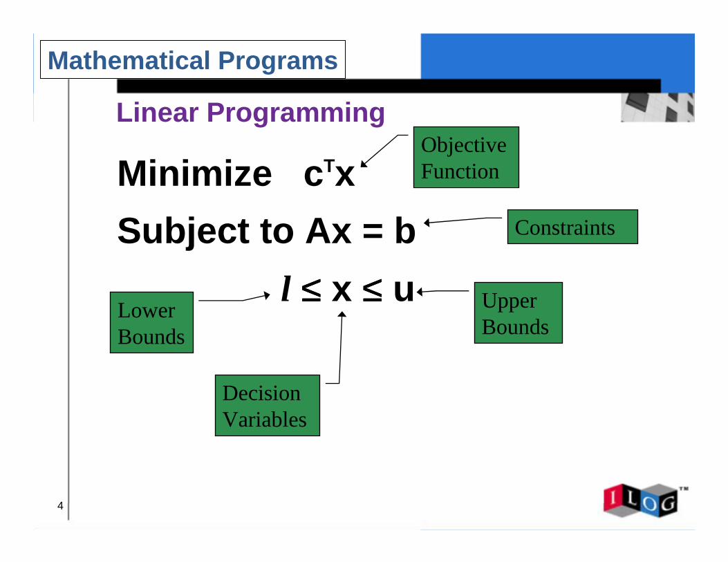
Linear Programming

Minimize cTxSubject to Ax = b

l ≤≤≤≤ x ≤≤≤≤ u

Objective Function

Constraints

Decision Variables

Lower Bounds

Upper Bounds

Mathematical Programs

5

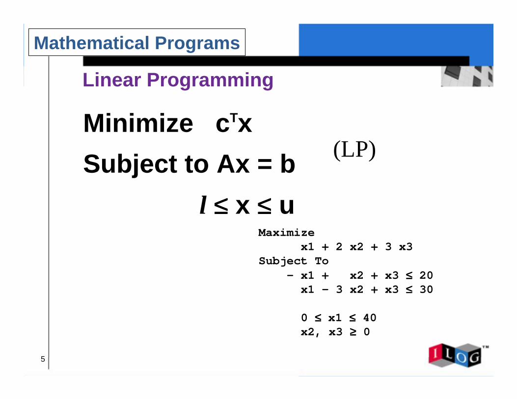
Linear Programming


l ≤≤≤≤ x ≤≤≤≤ u

(LP)

Maximizex1 + 2 x2 + 3 x3

Subject To- x1 + x2 + x3 ≤≤≤≤ 20x1 - 3 x2 + x3 ≤≤≤≤ 30

0 ≤≤≤≤ x1 ≤≤≤≤ 40x2, x3 ≥≥≥≥ 0


6

Linear Programming

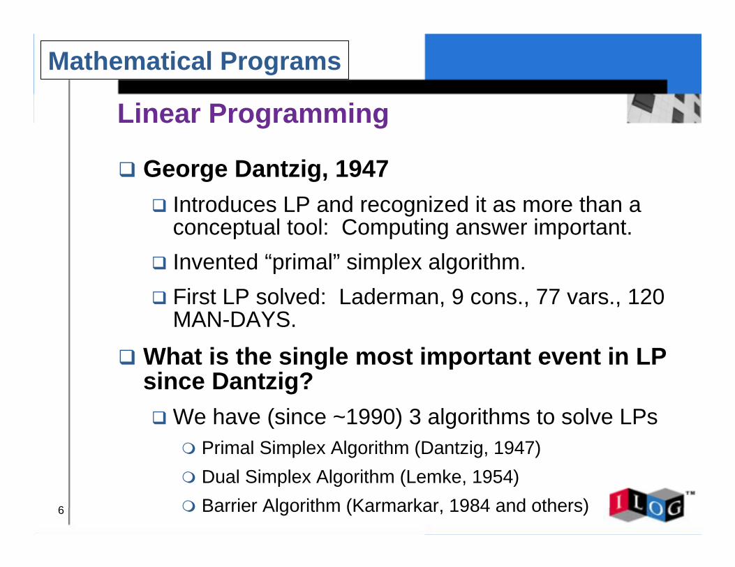
! George Dantzig, 1947! Introduces LP and recognized it as more than a

conceptual tool: Computing answer important.! Invented “primal” simplex algorithm.! First LP solved: Laderman, 9 cons., 77 vars., 120

MAN-DAYS.! What is the single most important event in LP

since Dantzig? ! We have (since ~1990) 3 algorithms to solve LPs

" Primal Simplex Algorithm (Dantzig, 1947)" Dual Simplex Algorithm (Lemke, 1954)" Barrier Algorithm (Karmarkar, 1984 and others)


7

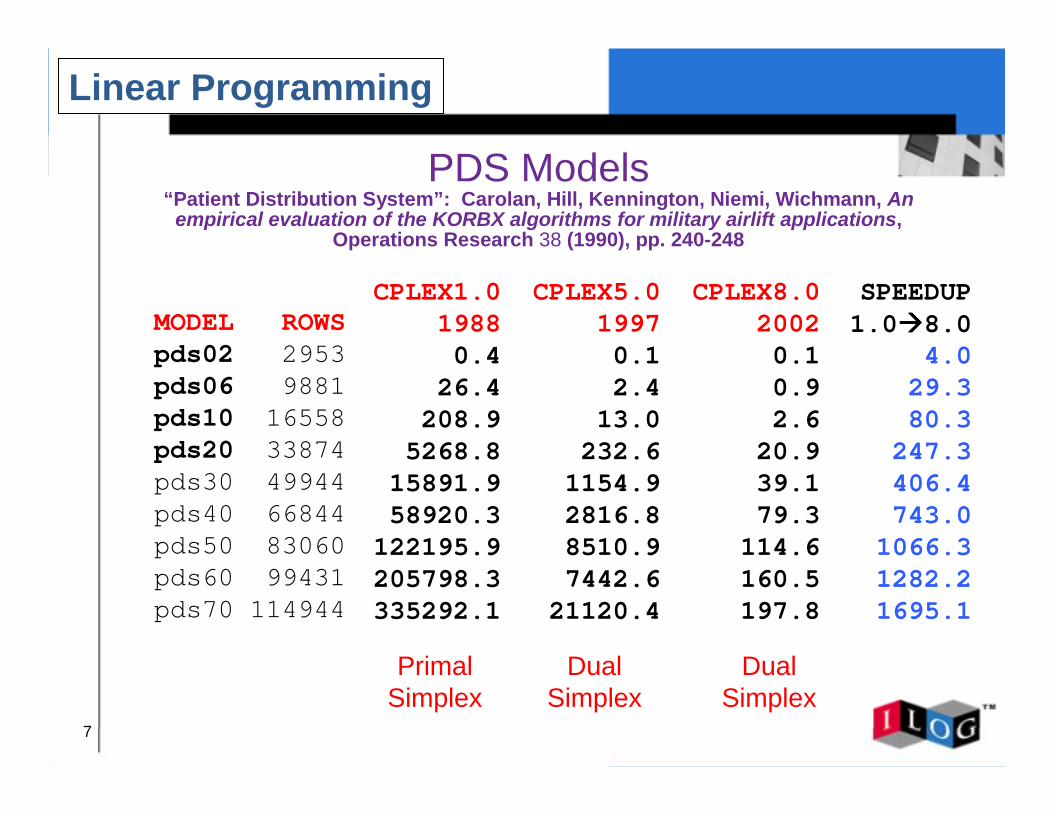
PDS Models“Patient Distribution System”: Carolan, Hill, Kennington, Niemi, Wichmann, An

empirical evaluation of the KORBX algorithms for military airlift applications, Operations Research 38 (1990), pp. 240-248

MODEL ROWSpds02 2953pds06 9881pds10 16558pds20 33874pds30 49944pds40 66844 pds50 83060pds60 99431pds70 114944

CPLEX1.019880.4 26.4 208.9 5268.8 15891.9 58920.3 122195.9 205798.3 335292.1

CPLEX5.0 19970.1 2.4 13.0 232.6 1154.9 2816.8 8510.9 7442.6 21120.4

CPLEX8.0 20020.1 0.9 2.6 20.9 39.1 79.3 114.6 160.5 197.8

SPEEDUP1.0####8.0

4.029.380.3 247.3406.4743.01066.31282.21695.1

PrimalSimplex

DualSimplex

DualSimplex

Linear Programming

8

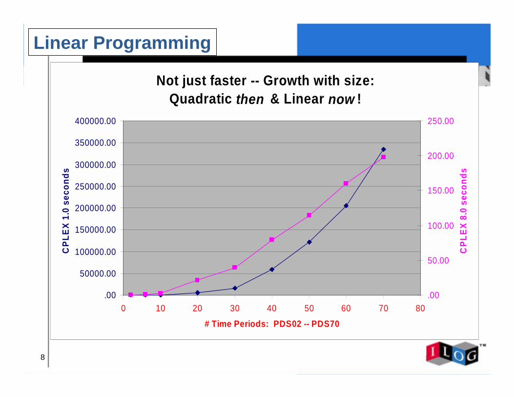
Not just faster -- Growth with size:Quadratic then & Linear now !

.00

50000.00

100000.00

150000.00

200000.00

250000.00

300000.00

350000.00

400000.00

0 10 20 30 40 50 60 70 80

# Time Periods: PDS02 -- PDS70

CPL

EX 1

.0 s

econ

ds

.00

50.00

100.00

150.00

200.00

250.00

CPL

EX 8

.0 s

econ

ds

Linear Programming

9

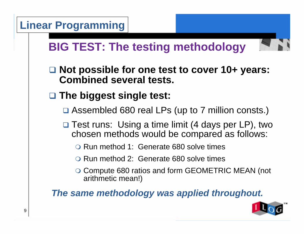
The same methodology was applied throughout.

Linear Programming

BIG TEST: The testing methodology

! Not possible for one test to cover 10+ years: Combined several tests.

! The biggest single test:! Assembled 680 real LPs (up to 7 million consts.)! Test runs: Using a time limit (4 days per LP), two

chosen methods would be compared as follows:" Run method 1: Generate 680 solve times" Run method 2: Generate 680 solve times" Compute 680 ratios and form GEOMETRIC MEAN (not

arithmetic mean!)

10

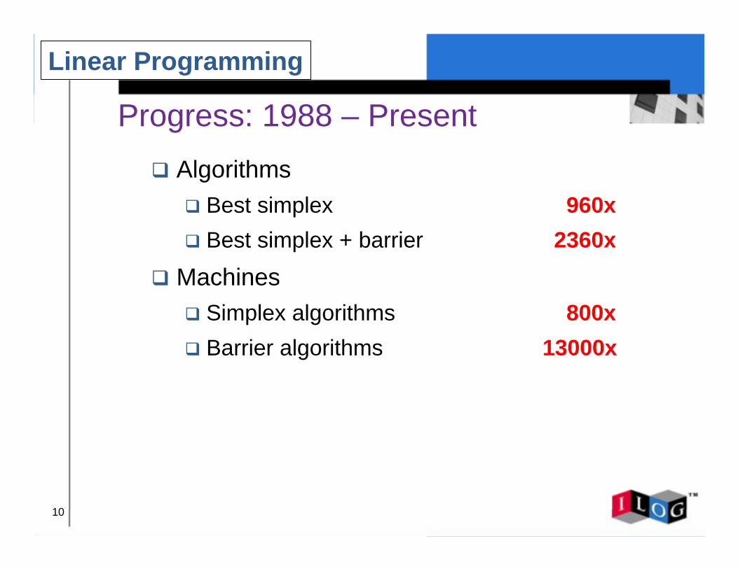
Progress: 1988 – Present! Algorithms

! Best simplex 960x! Best simplex + barrier 2360x

! Machines! Simplex algorithms 800x! Barrier algorithms 13000x

Linear Programming

11

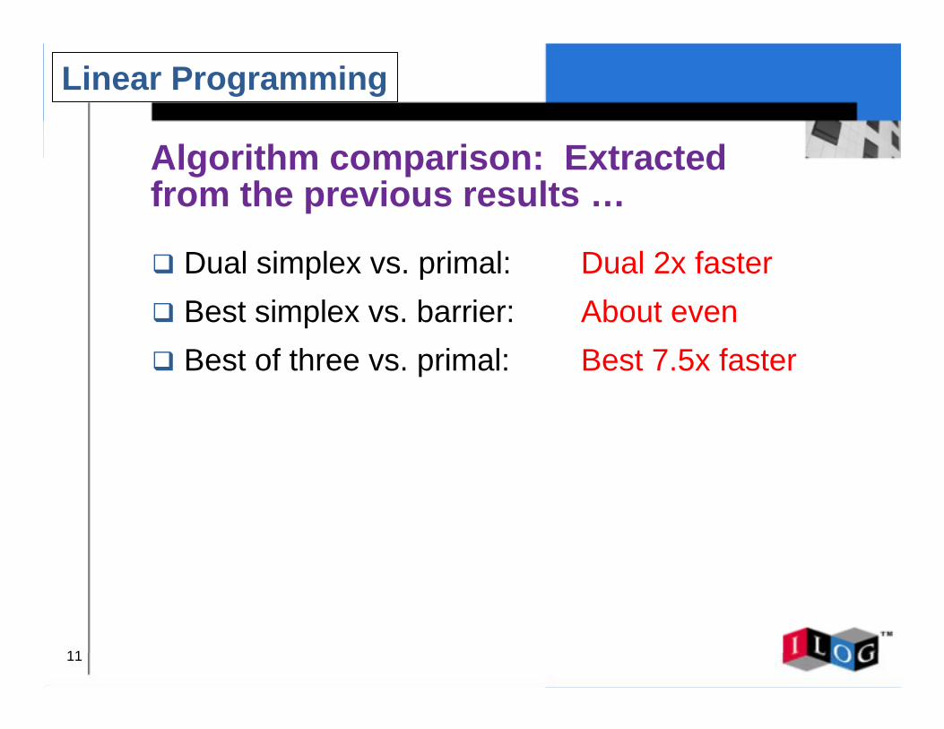
Algorithm comparison: Extracted from the previous results …

! Dual simplex vs. primal: Dual 2x faster! Best simplex vs. barrier: About even! Best of three vs. primal: Best 7.5x faster

Linear Programming

12

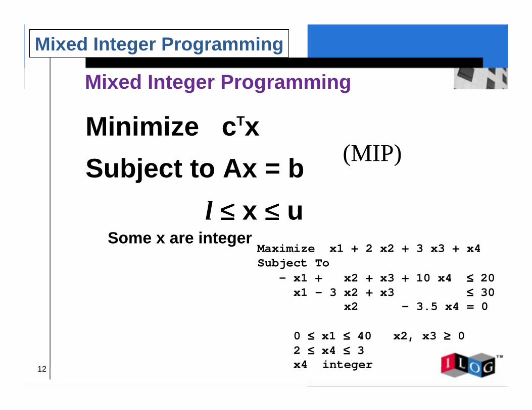
Maximize x1 + 2 x2 + 3 x3 + x4Subject To

- x1 + x2 + x3 + 10 x4 ≤≤≤≤ 20x1 - 3 x2 + x3 ≤≤≤≤ 30

x2 - 3.5 x4 = 0

0 ≤≤≤≤ x1 ≤≤≤≤ 40 x2, x3 ≥≥≥≥ 02 ≤≤≤≤ x4 ≤≤≤≤ 3x4 integer

(MIP)

Mixed Integer Programming


l ≤≤≤≤ x ≤≤≤≤ uSome x are integer


13

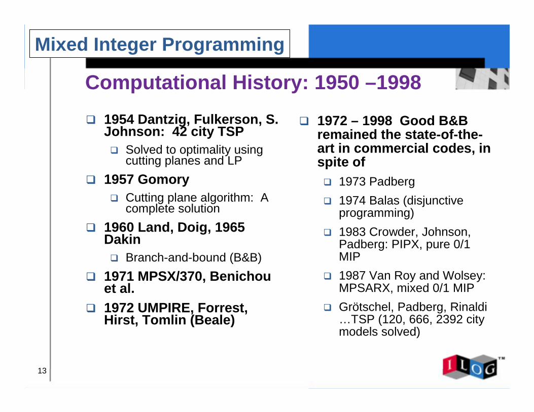
Computational History: 1950 –1998! 1954 Dantzig, Fulkerson, S.

Johnson: 42 city TSP! Solved to optimality using

cutting planes and LP! 1957 Gomory

! Cutting plane algorithm: A complete solution

! 1960 Land, Doig, 1965 Dakin! Branch-and-bound (B&B)

! 1971 MPSX/370, Benichou et al.

! 1972 UMPIRE, Forrest, Hirst, Tomlin (Beale)

! 1972 – 1998 Good B&B remained the state-of-the-art in commercial codes, in spite of! 1973 Padberg! 1974 Balas (disjunctive

programming)! 1983 Crowder, Johnson,

Padberg: PIPX, pure 0/1 MIP

! 1987 Van Roy and Wolsey: MPSARX, mixed 0/1 MIP

! Grötschel, Padberg, Rinaldi…TSP (120, 666, 2392 city models solved)


14


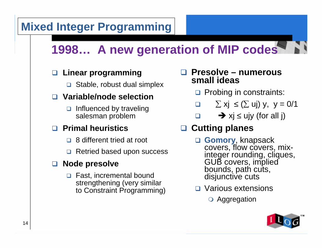
1998… A new generation of MIP codes

! Linear programming! Stable, robust dual simplex

! Variable/node selection! Influenced by traveling

salesman problem

! Primal heuristics ! 8 different tried at root ! Retried based upon success

! Node presolve! Fast, incremental bound

strengthening (very similar to Constraint Programming)

! Presolve – numerous small ideas! Probing in constraints: ! ∑ xj ≤ (∑ uj) y, y = 0/1! $ xj ≤ ujy (for all j)

! Cutting planes! Gomory, knapsack

covers, flow covers, mix-integer rounding, cliques, GUB covers, implied bounds, path cuts, disjunctive cuts

! Various extensions" Aggregation

15

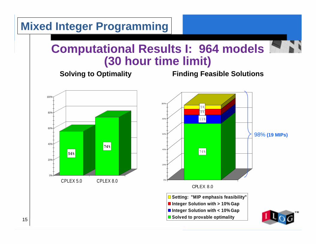
Computational Results I: 964 models(30 hour time limit)

74%

11%

8%5%

0%

20%

40%

60%

80%

100%

CPLEX 8.0

Setting: "MIP emphasis feasibility"Integer Solution with > 10% GapInteger Solution with < 10% GapSolved to provable optimality

56%

74%

0%

20%

40%

60%

80%

100%

CPLEX 5.0 CPLEX 8.0

Solving to Optimality Finding Feasible Solutions

98% (19 MIPs)


16

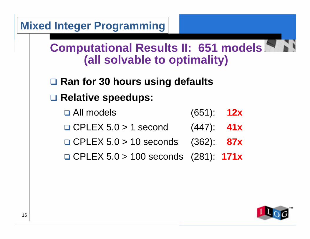
Computational Results II: 651 models (all solvable to optimality)

! Ran for 30 hours using defaults! Relative speedups:

! All models (651): 12x! CPLEX 5.0 > 1 second (447): 41x! CPLEX 5.0 > 10 seconds (362): 87x! CPLEX 5.0 > 100 seconds (281): 171x


17


Summary of Progress

! Through a combination of advances in algorithms and computing machines, combined with developments in data availability and modern modeling languages, what is possible today could only have been dreamed of even 10 years ago.

! The result is that whole new application domains have been enabled! Larger, more accurate models and multiple scenarios! Tactical and day-of-operations are possible, not just planning! Disparate components of the extended enterprise can now be

“optimized” in concert.

18

Constraint Programming

19

Problem Definition

! Minimize (or maximize) an Objective Function! Subject to Constraints! Over a set of values of Decision Variables

! Usual Requirements! Objective function and constraints have closed

mathematical forms (linear, quadratic, nonlinear, etc.)

! Decision variables are real or integer-valued" Each variable takes values over an interval


20


Problem Types

! Linear Program! (Mixed) Integer Program! Quadratic Program! Nonlinear Program! ...

A program is a problem

21


Computer Programming

! Knuth, 1968, The Art of Computer Programming! “An expression of a computational method in a

computer language is called a program.”! Programming Paradigms

! Procedural Programming! Object-oriented Programming! Functional Programming! Logic Programming! ....

22

Definition

! A computer programming methodology! Solves

! Constraint satisfaction problems! Combinatorial optimization problems

! Methodology! Represent a model of a problem in a computer

programming language! Describe a search strategy for solving the problem


23

Constraint Satisfaction Problems

! Find a Feasible Solution! Subject to Constraints! Over a set of values of Decision Variables

! Usual Requirements! Constraints are easy to evaluate

" Closed mathematical forms or table lookups

! Decision variables are values over a discrete set


24

Combinatorial Optimization Problems

! Minimize (or maximize) an Objective Function! Subject to Constraints! Over a set of values of Decision Variables

! Usual Requirements! Objective Function and Constraints are easy to

evaluate" Closed mathematical forms or table lookups

! Decision variables are values over a discrete set


25

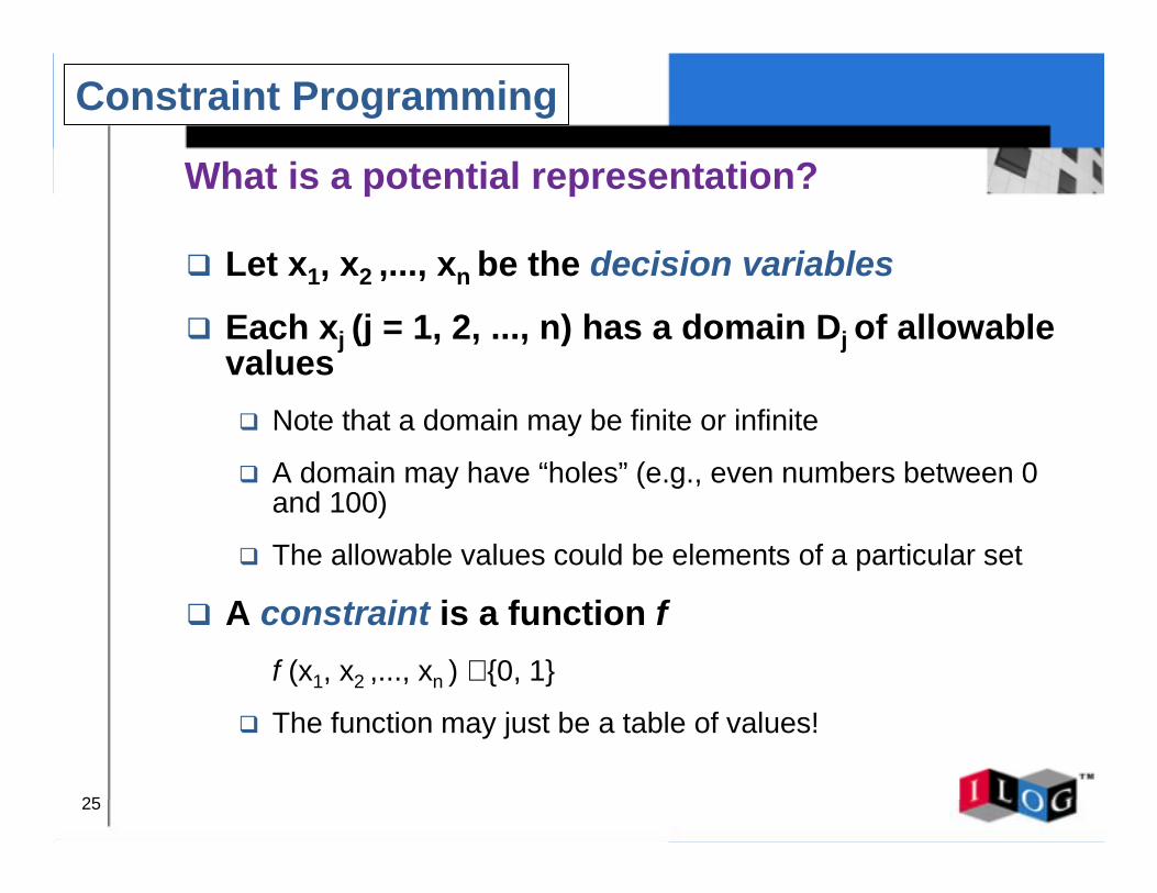
What is a potential representation?

! Let x1, x2 ,..., xn be the decision variables

! Each xj (j = 1, 2, ..., n) has a domain Dj of allowable values! Note that a domain may be finite or infinite

! A domain may have “holes” (e.g., even numbers between 0 and 100)

! The allowable values could be elements of a particular set

! A constraint is a function ff (x1, x2 ,..., xn ) ∈ {0, 1}

! The function may just be a table of values!


26

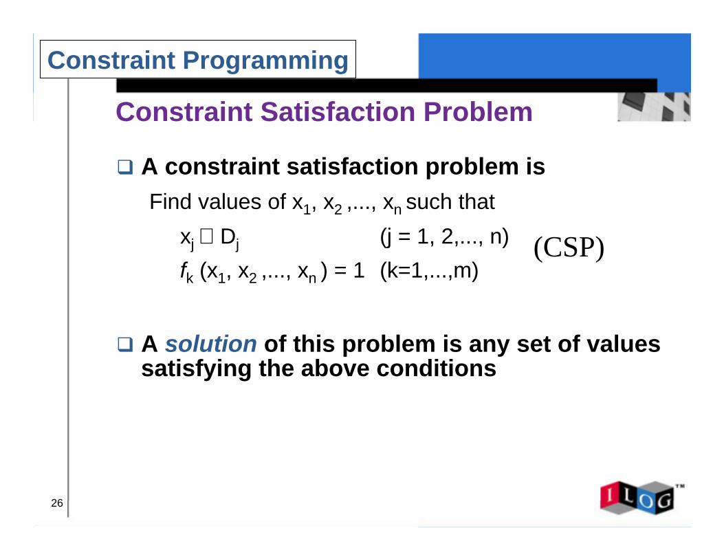
Constraint Satisfaction Problem

! A constraint satisfaction problem is Find values of x1, x2 ,..., xn such that

xj ∈ Dj (j = 1, 2,..., n)fk (x1, x2 ,..., xn ) = 1 (k=1,...,m)

! A solution of this problem is any set of values satisfying the above conditions

(CSP)


27


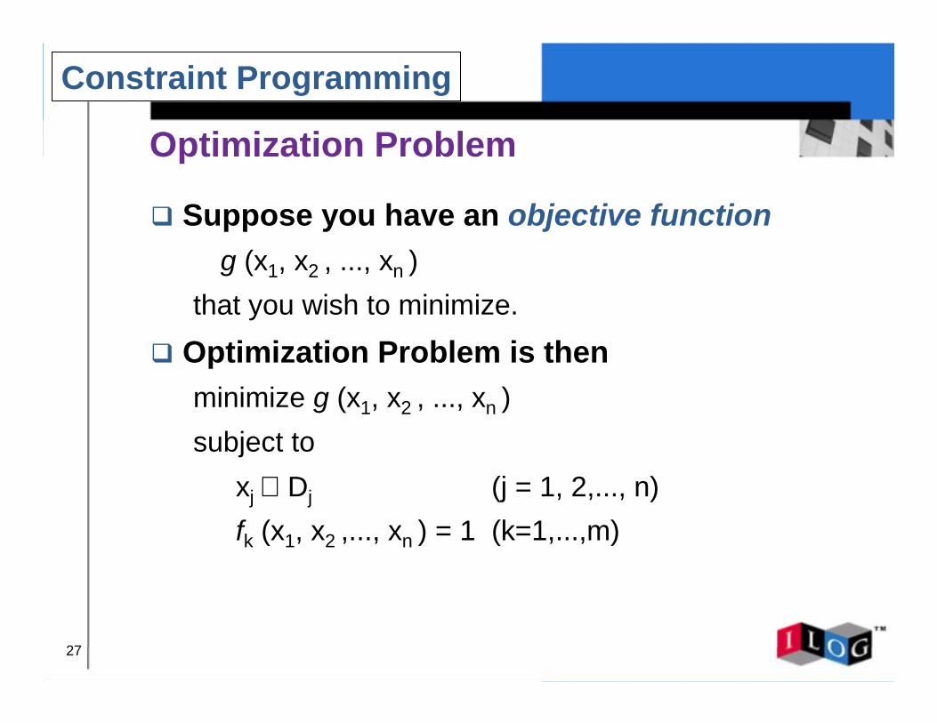
Optimization Problem

! Suppose you have an objective functiong (x1, x2 , ..., xn )

that you wish to minimize.! Optimization Problem is then

minimize g (x1, x2 , ..., xn )subject to

xj ∈ Dj (j = 1, 2,..., n)fk (x1, x2 ,..., xn ) = 1 (k=1,...,m)

28


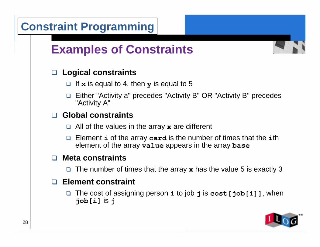
Examples of Constraints

! Logical constraints! If x is equal to 4, then y is equal to 5! Either "Activity a" precedes "Activity B" OR "Activity B" precedes

"Activity A"

! Global constraints! All of the values in the array x are different! Element i of the array card is the number of times that the ith

element of the array value appears in the array base

! Meta constraints! The number of times that the array x has the value 5 is exactly 3

! Element constraint! The cost of assigning person i to job j is cost[job[i]], when

job[i] is j

29

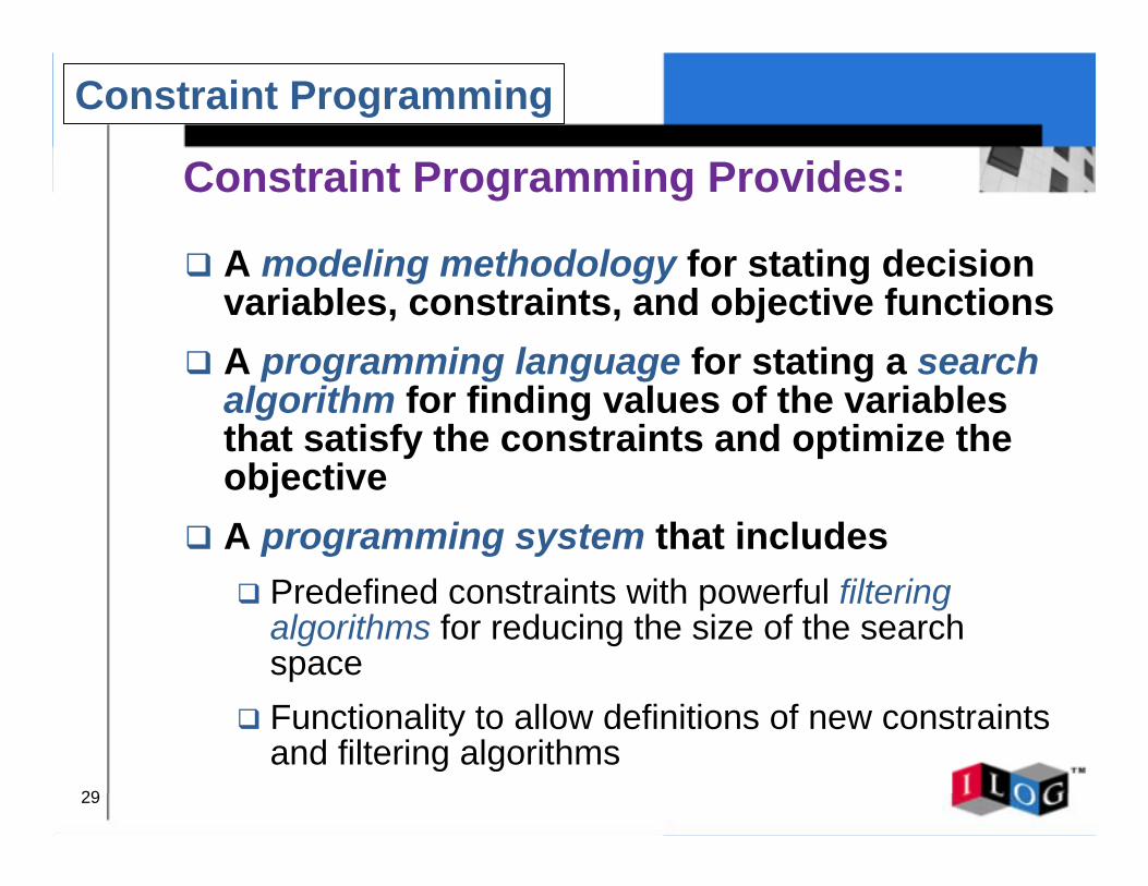
Constraint Programming Provides:

! A modeling methodology for stating decision variables, constraints, and objective functions

! A programming language for stating a search algorithm for finding values of the variables that satisfy the constraints and optimize the objective

! A programming system that includes! Predefined constraints with powerful filtering

algorithms for reducing the size of the search space

! Functionality to allow definitions of new constraints and filtering algorithms


30

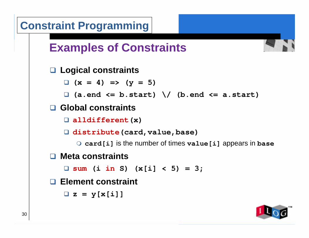
Examples of Constraints

! Logical constraints! (x = 4) => (y = 5)

! (a.end <= b.start) \/ (b.end <= a.start)

! Global constraints! alldifferent(x)

! distribute(card,value,base)

" card[i] is the number of times value[i] appears in base

! Meta constraints! sum (i in S) (x[i] < 5) = 3;

! Element constraint! z = y[x[i]]


31

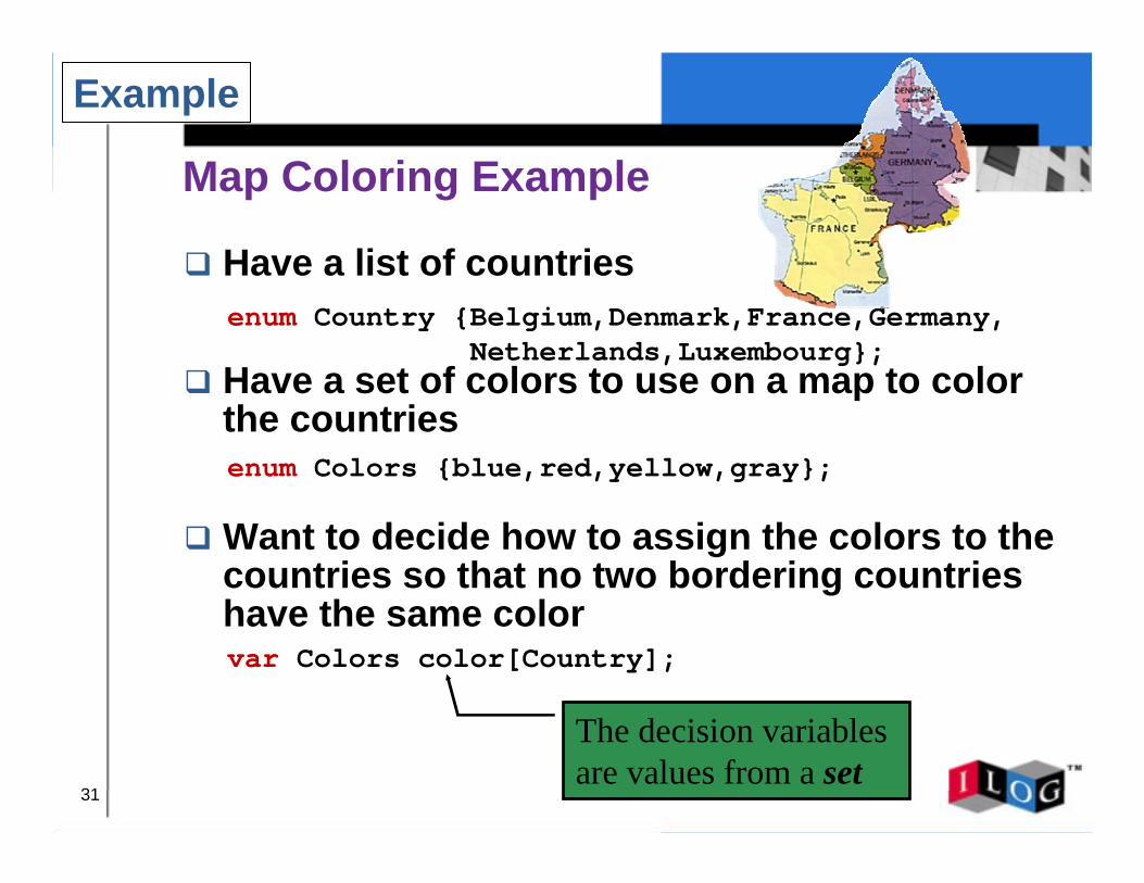
! Have a list of countries

! Have a set of colors to use on a map to color the countries

! Want to decide how to assign the colors to the countries so that no two bordering countries have the same color

enum Country {Belgium,Denmark,France,Germany,Netherlands,Luxembourg};

enum Colors {blue,red,yellow,gray};

var Colors color[Country];

The decision variables are values from a set

Map Coloring Example

Example

32

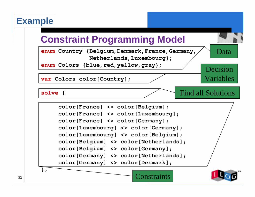
enum Country {Belgium,Denmark,France,Germany,Netherlands,Luxembourg};

enum Colors {blue,red,yellow,gray};


solve {

color[France] <> color[Belgium];color[France] <> color[Luxembourg];color[France] <> color[Germany];color[Luxembourg] <> color[Germany];color[Luxembourg] <> color[Belgium];color[Belgium] <> color[Netherlands];color[Belgium] <> color[Germany];color[Germany] <> color[Netherlands];color[Germany] <> color[Denmark];

};

Find all Solutions

Constraints

Data

DecisionVariables

Constraint Programming Model

Example

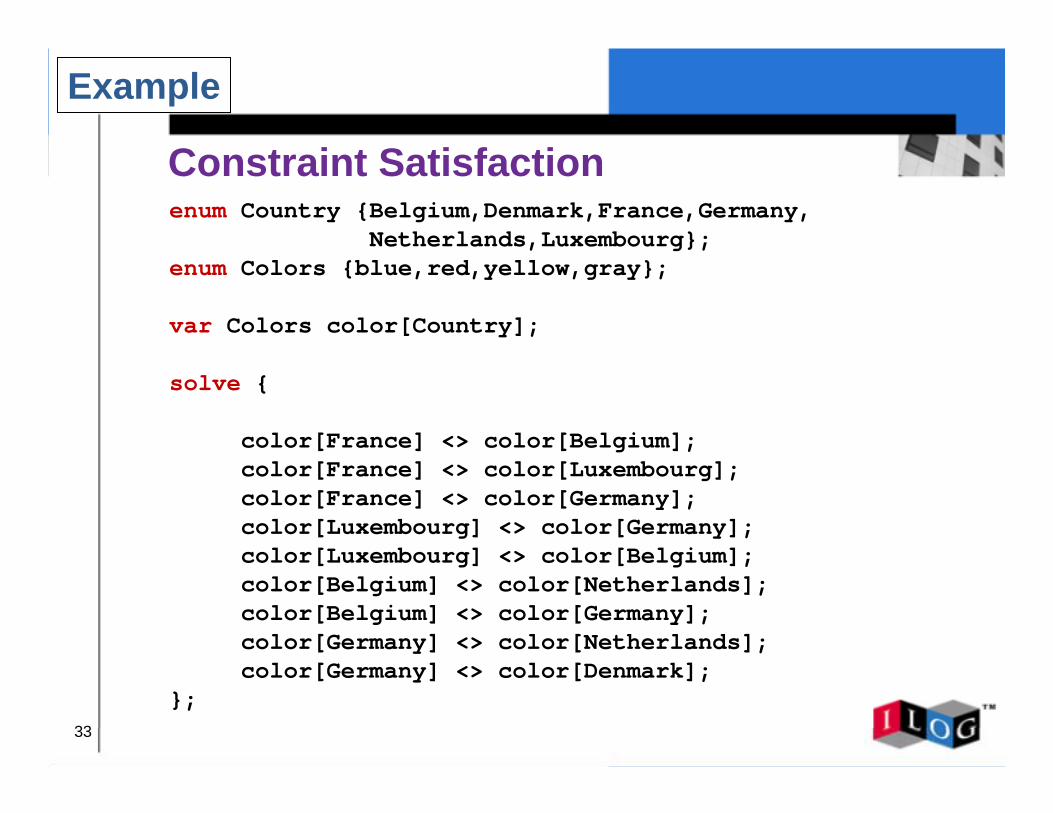
33

Constraint Satisfactionenum Country {Belgium,Denmark,France,Germany,

Netherlands,Luxembourg};enum Colors {blue,red,yellow,gray};


solve {

color[France] <> color[Belgium];color[France] <> color[Luxembourg];color[France] <> color[Germany];color[Luxembourg] <> color[Germany];color[Luxembourg] <> color[Belgium];color[Belgium] <> color[Netherlands];color[Belgium] <> color[Germany];color[Germany] <> color[Netherlands];color[Germany] <> color[Denmark];

};

Example

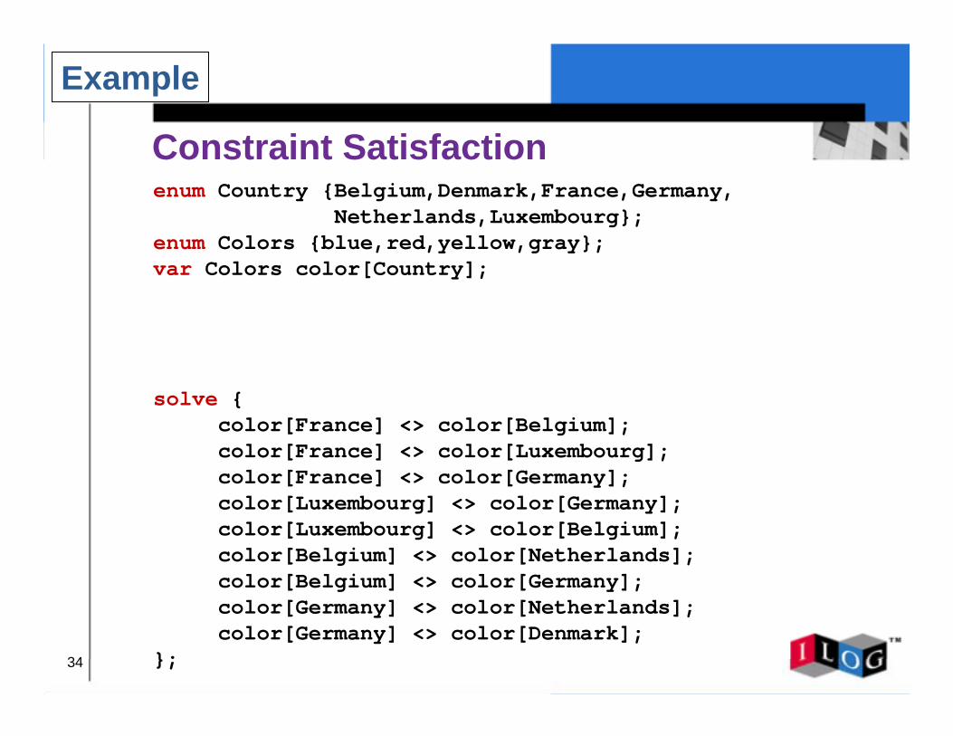
34

Constraint Satisfactionenum Country {Belgium,Denmark,France,Germany,

Netherlands,Luxembourg};enum Colors {blue,red,yellow,gray};var Colors color[Country];

solve {color[France] <> color[Belgium];color[France] <> color[Luxembourg];color[France] <> color[Germany];color[Luxembourg] <> color[Germany];color[Luxembourg] <> color[Belgium];color[Belgium] <> color[Netherlands];color[Belgium] <> color[Germany];color[Germany] <> color[Netherlands];color[Germany] <> color[Denmark];

};

Example

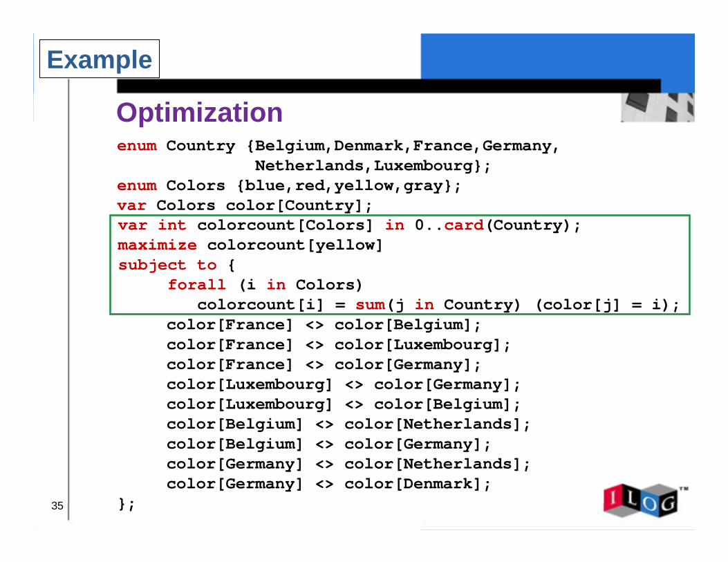
35

Optimizationenum Country {Belgium,Denmark,France,Germany,

Netherlands,Luxembourg};enum Colors {blue,red,yellow,gray};var Colors color[Country];

solve {color[France] <> color[Belgium];color[France] <> color[Luxembourg];color[France] <> color[Germany];color[Luxembourg] <> color[Germany];color[Luxembourg] <> color[Belgium];color[Belgium] <> color[Netherlands];color[Belgium] <> color[Germany];color[Germany] <> color[Netherlands];color[Germany] <> color[Denmark];

};

var int colorcount[Colors] in 0..card(Country);maximize colorcount[yellow]subject to {

forall (i in Colors) colorcount[i] = sum(j in Country) (color[j] = i);

Example

36

Problem Description

! From Bradley, Hax, Magnanti, Applied Mathematical Programming, Chapter 9, Exercise 24! Custom Pilot Chemical Company is a chemical manufacturer that produces

batches of specialty chemicals to order. Principal equipment consists of eight interchangable reactor vessels, five interchangeable distillation columns, four large interchangeable centrifuges, and a network of switchable piping and storage tanks. Customer demand comes in the form of orders for batches of one or more specialty chemicals, normally to be delivered simultaneously for further use by the customer.

! An order consists of a set of jobs. Each job has an optional precedence requirement, arrival week of the job, duration of the job in weeks, the week that the job is due, the number of reactors required, distillation columns required, and centrifuges required.

! Find a schedule of the orders and jobs to minimize the completion time of all orders

Production Scheduling

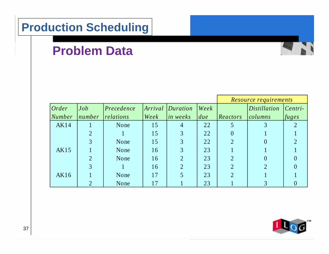
37

Problem Data

Order Number

Job number

Precedence relations

Arrival Week

Duration in weeks

Week due Reactors

Distillation columns

Centri-fuges

AK14 1 None 15 4 22 5 3 22 1 15 3 22 0 1 13 None 15 3 22 2 0 2

AK15 1 None 16 3 23 1 1 12 None 16 2 23 2 0 03 1 16 2 23 2 2 0

AK16 1 None 17 5 23 2 1 12 None 17 1 23 1 3 0

Resource requirements


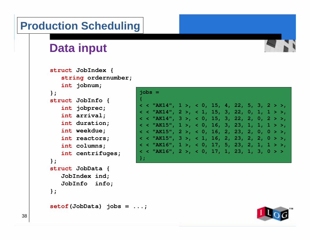
38

Data inputstruct JobIndex {

string ordernumber;int jobnum;

};struct JobInfo {

int jobprec;int arrival;int duration;int weekdue;int reactors;int columns;int centrifuges;

};struct JobData {

JobIndex ind;JobInfo info;

};

setof(JobData) jobs = ...;

jobs ={< < "AK14", 1 >, < 0, 15, 4, 22, 5, 3, 2 > >,< < "AK14", 2 >, < 1, 15, 3, 22, 0, 1, 1 > >,< < "AK14", 3 >, < 0, 15, 3, 22, 2, 0, 2 > >,< < "AK15", 1 >, < 0, 16, 3, 23, 1, 1, 1 > >,< < "AK15", 2 >, < 0, 16, 2, 23, 2, 0, 0 > >,< < "AK15", 3 >, < 1, 16, 2, 23, 2, 2, 0 > >,< < "AK16", 1 >, < 0, 17, 5, 23, 2, 1, 1 > >,< < "AK16", 2 >, < 0, 17, 1, 23, 1, 3, 0 > >};


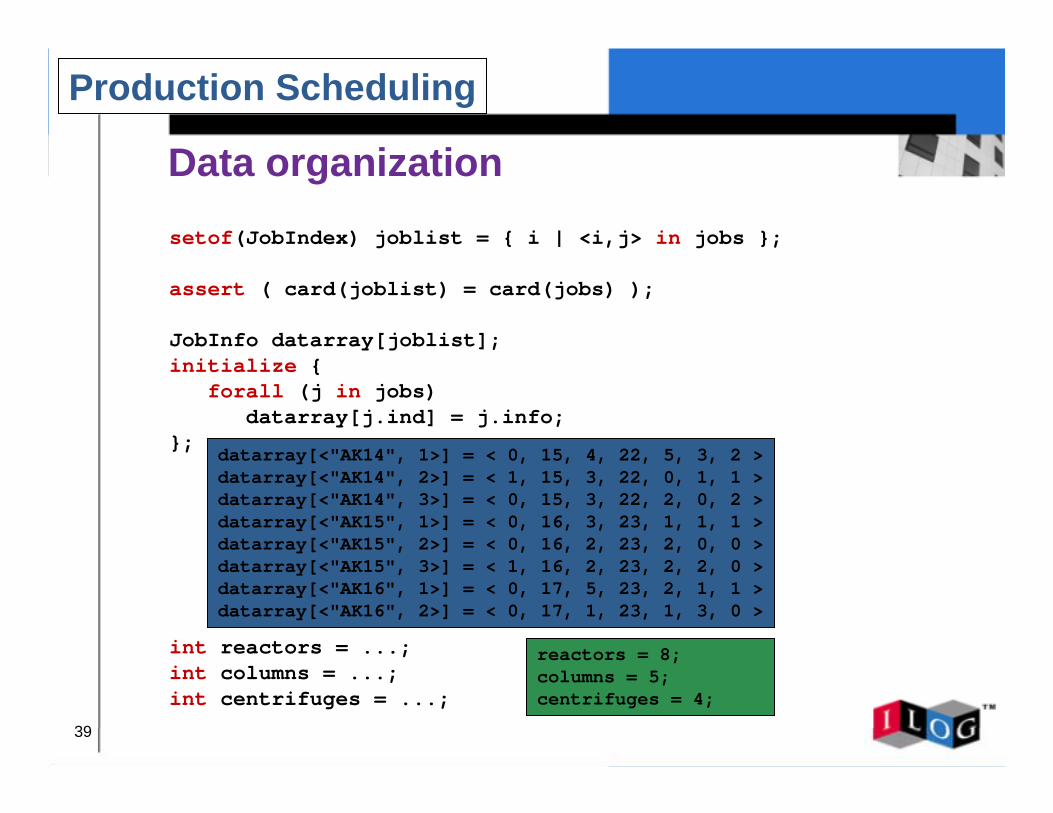
39

Data organizationsetof(JobIndex) joblist = { i | <i,j> in jobs };

assert ( card(joblist) = card(jobs) );

JobInfo datarray[joblist];initialize {

forall (j in jobs) datarray[j.ind] = j.info;

};

int reactors = ...;int columns = ...;int centrifuges = ...;

datarray[<"AK14", 1>] = < 0, 15, 4, 22, 5, 3, 2 >datarray[<"AK14", 2>] = < 1, 15, 3, 22, 0, 1, 1 >datarray[<"AK14", 3>] = < 0, 15, 3, 22, 2, 0, 2 >datarray[<"AK15", 1>] = < 0, 16, 3, 23, 1, 1, 1 >datarray[<"AK15", 2>] = < 0, 16, 2, 23, 2, 0, 0 >datarray[<"AK15", 3>] = < 1, 16, 2, 23, 2, 2, 0 >datarray[<"AK16", 1>] = < 0, 17, 5, 23, 2, 1, 1 >datarray[<"AK16", 2>] = < 0, 17, 1, 23, 1, 3, 0 >

reactors = 8;columns = 5;centrifuges = 4;


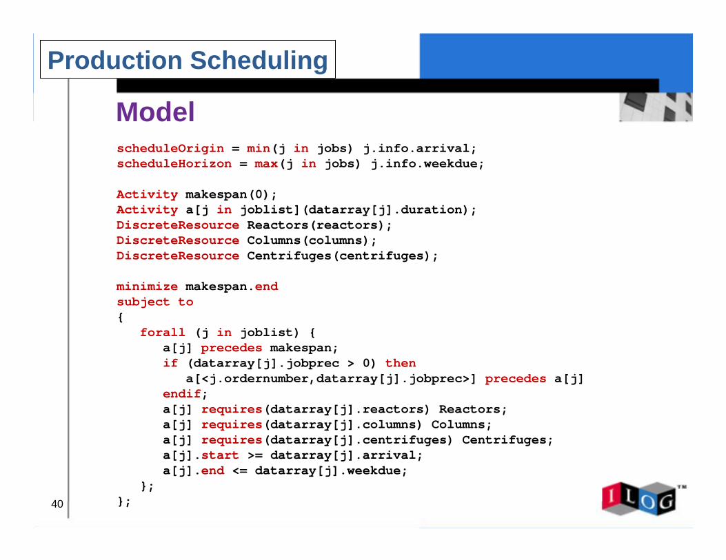
40

ModelscheduleOrigin = min(j in jobs) j.info.arrival;scheduleHorizon = max(j in jobs) j.info.weekdue;

Activity makespan(0);Activity a[j in joblist](datarray[j].duration);DiscreteResource Reactors(reactors);DiscreteResource Columns(columns);DiscreteResource Centrifuges(centrifuges);

minimize makespan.endsubject to{

forall (j in joblist) {a[j] precedes makespan;if (datarray[j].jobprec > 0) then

a[<j.ordernumber,datarray[j].jobprec>] precedes a[j]endif;a[j] requires(datarray[j].reactors) Reactors;a[j] requires(datarray[j].columns) Columns;a[j] requires(datarray[j].centrifuges) Centrifuges;a[j].start >= datarray[j].arrival;a[j].end <= datarray[j].weekdue;

};};


41

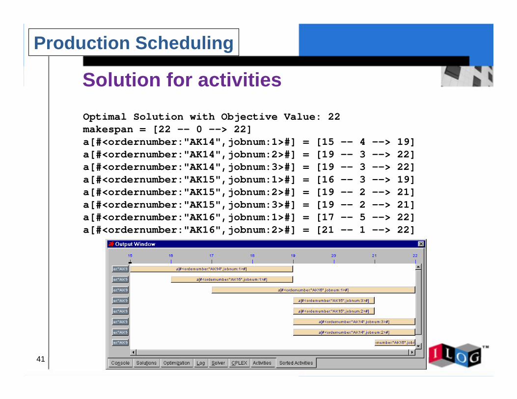
Solution for activitiesOptimal Solution with Objective Value: 22makespan = [22 -- 0 --> 22]a[#<ordernumber:"AK14",jobnum:1>#] = [15 -- 4 --> 19]a[#<ordernumber:"AK14",jobnum:2>#] = [19 -- 3 --> 22]a[#<ordernumber:"AK14",jobnum:3>#] = [19 -- 3 --> 22]a[#<ordernumber:"AK15",jobnum:1>#] = [16 -- 3 --> 19]a[#<ordernumber:"AK15",jobnum:2>#] = [19 -- 2 --> 21]a[#<ordernumber:"AK15",jobnum:3>#] = [19 -- 2 --> 21]a[#<ordernumber:"AK16",jobnum:1>#] = [17 -- 5 --> 22]a[#<ordernumber:"AK16",jobnum:2>#] = [21 -- 1 --> 22]


42

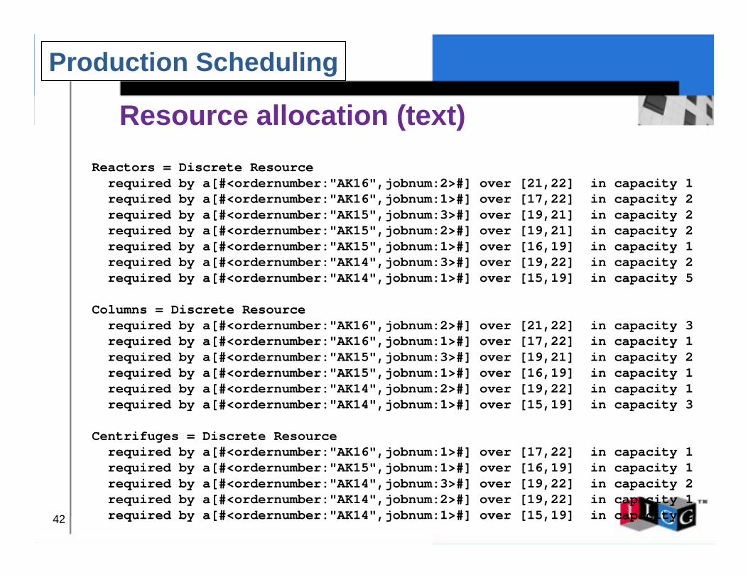
Resource allocation (text)Reactors = Discrete Resourcerequired by a[#<ordernumber:"AK16",jobnum:2>#] over [21,22] in capacity 1required by a[#<ordernumber:"AK16",jobnum:1>#] over [17,22] in capacity 2required by a[#<ordernumber:"AK15",jobnum:3>#] over [19,21] in capacity 2required by a[#<ordernumber:"AK15",jobnum:2>#] over [19,21] in capacity 2required by a[#<ordernumber:"AK15",jobnum:1>#] over [16,19] in capacity 1required by a[#<ordernumber:"AK14",jobnum:3>#] over [19,22] in capacity 2required by a[#<ordernumber:"AK14",jobnum:1>#] over [15,19] in capacity 5

Columns = Discrete Resourcerequired by a[#<ordernumber:"AK16",jobnum:2>#] over [21,22] in capacity 3required by a[#<ordernumber:"AK16",jobnum:1>#] over [17,22] in capacity 1required by a[#<ordernumber:"AK15",jobnum:3>#] over [19,21] in capacity 2required by a[#<ordernumber:"AK15",jobnum:1>#] over [16,19] in capacity 1required by a[#<ordernumber:"AK14",jobnum:2>#] over [19,22] in capacity 1required by a[#<ordernumber:"AK14",jobnum:1>#] over [15,19] in capacity 3

Centrifuges = Discrete Resourcerequired by a[#<ordernumber:"AK16",jobnum:1>#] over [17,22] in capacity 1required by a[#<ordernumber:"AK15",jobnum:1>#] over [16,19] in capacity 1required by a[#<ordernumber:"AK14",jobnum:3>#] over [19,22] in capacity 2required by a[#<ordernumber:"AK14",jobnum:2>#] over [19,22] in capacity 1required by a[#<ordernumber:"AK14",jobnum:1>#] over [15,19] in capacity 2


43

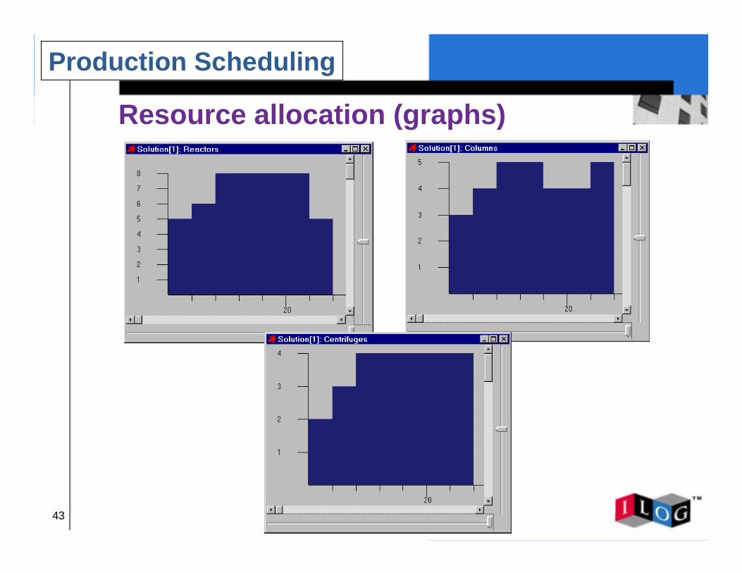
Resource allocation (graphs)


44

Which is BETTER????

! It depends upon the data! It depends on the search strategy! It depends on the combinatorial nature of the

problem

! For general applications, you need tools that allow you to try both methodologies!

Comparing CP and MP

45

What is a solution?

! Linear programs and integer programs always have objective functions

! A constraint satisfaction problem may simply be a feasibility problem! It may have many possible solutions!

! People in constraint programming say that they have a “solution” when people in mathematical programming would say they have a “feasible solution”

Comparing CP and MP

46

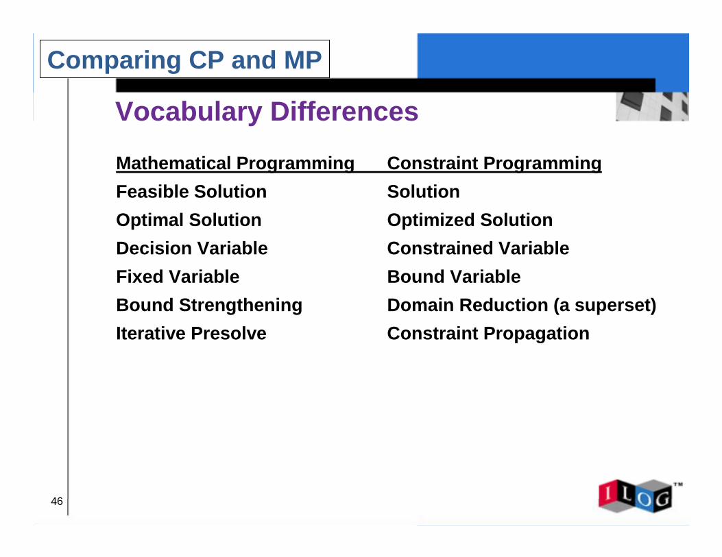
Vocabulary Differences

Mathematical Programming Constraint ProgrammingFeasible Solution SolutionOptimal Solution Optimized SolutionDecision Variable Constrained VariableFixed Variable Bound VariableBound Strengthening Domain Reduction (a superset)Iterative Presolve Constraint Propagation

Comparing CP and MP

47

Constraint Programming Successes

48

! Centralized Vehicle Scheduler: for vehicle production

! Results: Competitive advantage & savings! 10-20% improvement in purge rates! Increased production by 4,000 cars/year/plant! Estimated savings of $27 million annually

DaimlerChryslerOptimization Successes

49

! Loan Arranger: Searches for loan that best meets each customer’s requirements

! Results: Competitive advantage & savings! 4 x increase in monthly loan volume! 15% increase in average loan size! Reduced “time to funding” from 21 to 8 days! Reduced underwriting costs by 78%

First Union

Optimization Successes

50

SNCF Railways

! Rolling Stock Maintenance Operations! Schedule Operations Efficiently! Save 10% of 2,000 maintenance workers


51

Nissan (UK)

! Challenge: Build 3rd car model with 2 existing production lines

! Results: Europe’s already most efficient car production facility is even more productive! No need to add any new production line and no

significant investment needed! Production capacity increased by 30%! Schedule adherence rose from 3% to 90%


52

Applications

! Scheduling! Dispatching! Configuration! Enumeration! Sequencing


53

Conclusions

! Optimization technologies have significantly improved over the past 15 years

! Multiple techniques! Traditional Mathematical Programming! Newer Constraint Programming

! An explosion of applications

Summary

Date post:	08-Mar-2018
Category:	Documents
Upload:	hadiep
View:	228 times
Download:	6 times

Progress in Linear and Integer Programming and...

Documents